Wisdom of Crowds vs. Groupthink:Learning in Groups and in Isolation

Conor Mayo-Wilson, Kevin Zollman, and David Danks

May 31, 2010

1 Introduction

In the multi-armed bandit problem, an individual is repeatedly faced with achoice between a number of potential actions, each of which yields a payoffdrawn from an unknown distribution. The agent wishes to maximize her totalaccumulated payoff (in the finite horizon case) or converge to an optimal actionin the limit (in the infinite horizon case). This very general model has been usedto model a variety of economic phenomena. For example, individuals choosingbetween competing technologies, like different computer platforms, would liketo maximize the total usefulness of the purchased technologies, but cannot knowahead of time how useful a particular technology will be. Others have suggestedapplying this model to the choice of treatments by doctors (Berry and Fristedt, 1985), crop choices in Africa (Bala and Goyal , 2008), and choice of drillingsites by oil companies (Keller, Rady, and Cripps , 2005).

The traditional analysis of strategies in bandit problems focuses on eithera known finite number of actions or a discounted infinite sequence of actions(cf. Berry and Fristedt , 1985). In both these cases, strategies are evaluatedaccording to their ability to maximize the (discounted) expected sum of pay-offs. Recent interest in boundedly rational strategies have led some scholars toconsider how strategies which do not maximize expected utility might perform.These strategies are evaluated according to their ability to converge in the in-finite limit to choosing the optimal action, without considering their short ormedium run behavior. For example, Beggs (2005) considers how a single indi-vidual who employs a reinforcement learning algorithm (due to Roth and Erev, 1995) would perform in a repeated multi-armed bandit problem.

Many of the above choice problems, like technology choice, are not madein isolation, but rather in a social context. A player can observe not only herown successes or failures, but those of some subset of the population of otherconsumers. As a result, several scholars have considered bandit problems insocial settings (Bolton and Harris , 1999; Bala and Goyal , 2008; Keller, Rady,and Cripps , 2005). Bala & Goyal, for example, consider a myopic Bayesianmaximizer placed in a population of other myopic Bayesian maximizers, andfind that certain structures for the communication of results ensures that this

1

community will converge to the optimal action, but other social structures willnot.

Although Beggs and Bala & Goyal seem to utilize essentially the same met-ric for the comparison of boundedly rational algorithms – convergence in thelimit – they are more different than they appear. Beggs considers how a sin-gle individual does when he plays a bandit in isolation; Bala & Goyal considerhow a group fares when in a specific circumstance. It should be clear that themyopic maximizer of Bala & Goyal would not converge in the limit if he was inisolation. It is perhaps less clear that Beggs’ reinforcement learner might notconverge if placed in the wrong social circumstance.

This paper considers two different, but closely related, problems raised bythese types of investigations. First, we wish to understand how a variety ofdifferent boundedly rational strategies perform on multi-armed bandit problemsplayed both in isolation and within a community. We consider a very generalmulti-armed bandit problem and compare the performance of several differentclasses of boundedly rational learning rules. Second, we wish to make precise thenotion of a strategy being convergent in the limit. In particular we will considerdifferent answers to the questions (a) are we considering the strategy in totalisolation or when placed in a social circumstance; and (b) are we considering onlya single strategy or a set of strategies? We find that which boundedly rationalstrategies are judged as appropriate depends critically on how one answers thesequestions. This, we believe, makes perspicuous the choices one must make beforeengaging in the analysis of various boundedly rational strategies.

In section 2 we provide the details of our model of bandit problems and fourgeneral classes of boundedly rational strategies. These four classes were chosento represent many of the strategies investigated in literatures in economics,psychology, computer science, and philosophy. Following this, we present thedifferent formalizations of the notion of convergence in the limit in section 3.Here we provide the theorems which demonstrate which strategies meet thevarious definitions, and illustrate that the different definitions are distinct fromone another. Section 4 concludes with a discussion of the applications andpotential extensions of the results presented here.

2 The model of learning

We begin by modeling individual agents as embedded in a communication net-work. The communication network will be represented by a finite, undirectedgraph G = 〈VG, EG〉 with vertices VG representing individual agents, and edgesEG representing pairs of agents who share information with one another. Wewill often write g ∈ G when we mean that g ∈ VG. By a similar abuse of no-tation, we use G′ ⊆ G to denote that G′ ⊆ VG. For any learner g ∈ G, defineNG(g) = g′ ∈ G : g, g′ ∈ EG to be the neighborhood of g in the networkG. We assume g ∈ NG(g) for all g ∈ G, so that each individual observesthe outcomes of her own choices. When the underlying network is clear fromcontext, we write N(g), dropping the subscript G.

2

In each time period, each agent chooses one of a finite number of actionsA. We assume that the set of actions is constant for all times, and each actionresults (probabilistically) in an outcome (or payoff) from a set O.1 There is a setΩ of possible states of the world which determine the probability distributionover O associated with each action.

A learning problem is a quadruple 〈Ω, A,O, p〉, where Ω is a set of states ofthe world, A is a finite set of actions, O is a finite set of real numbers calledoutcomes, and p is a probability measure specifying the probability of obtaininga particular utility given an action and state of the world.

A history specifies (at a given time period) the actions taken and outcomesreceived by every individual in the graph. Formally, for any set C, let C<N bethe set of all finite sequences with range in C. Then define the set H of possiblehistories as follows:

H = h ∈ ((A×O)<N)<N : |hn| = |hk| for all n, k ∈ N

where hn is the nth coordinate in the history h, i.e. hn is the sequence of actionsand outcomes obtained by some collection of learners at stage n of inquiry. Therequirement that |hn| = |hk| for all n, k ∈ N captures the fact that the size of agroup does not change over time. For a network G and a group G′ ⊆ G, define:

HG′,G = h ∈ H : |hn| = |G′| for all n ∈ N

When the network is clear from context, we will simply write HG′ to simplifynotation. Then HG is the set of network histories for the entire network, andHN(g) is the set of neighborhood histories for the learner g.

Example 1: Let G be the undirected graph with two vertices joined by anedge. Let Ω = ω1, ω2, A = a1, a2, O = 0, 1, and

p(1|ai, ωi) = .7 for i = j = 1, 2p(1|ai, ωj) = .1 for i 6= j

One can imagine A as possible drugs, outcomes 1 and 0 as respectively repre-senting that a patient is cured or not, and ωi as representing the state of theworld in which ai is the bettertreatment. A possible network history h ∈ HG

of length two is 〈〈〈a1, 1〉〈a1, 0〉〉, 〈〈a1, 0〉〈a2, 0〉〉〉, which denotes the history inwhich (i) one doctor applied treatment a1 to two successive patients, the first ofwhich was cured but the second of which was not, and (ii) a second doctor ap-plied treatment a1 to a patient who it failed to cure and then applied treatmenta2 to a second patient who was also uncured.

A method (also called a strategy) m for an agent is a function that specifies,for any particular history, a probability distribution over possible actions forthe next stage. In other words, a method specifies probabilities over the agent’sactions given what she knows about her own and her neighbors’ past actions and

1For technical reasons, we assume outcomes are non-negative, and that the set of outcomesis countable.

3

outcomes. Of course, an agent may act deterministically simply by placing unitprobability on a single action a ∈ A. A strategic network is a pair S = 〈G,M〉consisting of a network G and a sequence M = 〈mg〉g∈G specifying the strategyemployed by each learner, mg, in the network.

Together, a strategic network S = 〈G,M〉 and a learning problem 〈Ω, A,O, p〉determine a probability pSω(h) of any finite history h ∈ HG′ for any groupG′ ⊆ G. To see why, again consider Example 1. Suppose the two learnersboth employ the followingsimple strategy: if action ai led to a success 1 on theprevious stage, play it again with probability one; if the action failed, play theother action. Then the probability pSomega1

(h) of the history h in Example 1 instate of the world ω1 is

pSω1(h) = p(1|a1, ω1) · p(0|a1, ω1) · p(0|a1, ω1) · p(0|a2, ω1) = .7 · .3 · .3 · .9 = .1323

Notice, however, the same history h might have a different probability if onewere to respecify the methods employed by the agents in the network. Forexample, suppose the agents both employed the rule “switch actions if and onlyif a success is obtained.” Then the history h above would have probability zero(regardless of state of the world), as the first learner continues to play action a1

after a success.Because outcomes can be interpreted as utilities, it follows that for any

state of the world ω, there is an expected value Eω(a) of the action a that isconstant throughout time. Hence, in any state of the world ω, there is somecollection Aω = a ∈ A : Eω(a) ≥ Eω(a′) for all a′ ∈ A of optimal actionsthat maximize expected utility. Hence, it follows that the event that g plays anoptimal action at stage n has a well-defined probability, which we will denotepSω(hA(n, g) ∈ Aω). In the next section, we study the limiting behavior of suchprobabilities in various strategic networks.

Some learning problems are far easier than others; for example, if one actionhas higher expected utility in every world-state, then there is relatively littlefor the agents to learn. We are principally interestedin more difficult problems.Say a learning problem is non-trivial if no finite history reveals that a givenaction is optimal with certainty. In other words, a learning problem 〈Ω, A,O, p〉is non-trivial if for all strategic networks S = 〈G,M〉, and all network historiesh ∈ HG, if pSω1

(h) > 0 for some ω1 ∈ Ω, then there exists ω2 ∈ Ω such thatAω1 ∩ Aω2 = ∅ and pSω2

(h) > 0. Say a learning problem is difficult if it isnon-trivial, and 1 > p(0|a, ω) > 0 for all ω ∈ Ω and all a ∈ A. That is, noaction is guaranteed to succeed, and no history determines an optimal actionwith certainty.

2.1 Four Types of Strategies

Although the number of differing strategies is enormous, we will focus on thebehavior of four types of boundedly rational strategies: reinforcement learning(RL), simulated annealing (SA), decreasing ε-greedy (εG), and what we call, δεmethods. We study these strategies for four reasons. First, the first three types

4

of strategies have been employed extensively in economics, computer science,statistics, and many other disciplines in which one is interested in finding theglobal maximum (or minimum) of a utility (respectively, cost) function. Second,all four strategies are simple and algorithmic: they can easily be simulated oncomputers and, given enough discipline, performed by human beings. Third,the strategies have desirable asymptotic features in the sense that, in the limit,they find the global maximum of utility functions under robust assumptions.Fourth, some of the strategies have psychological plausibility as learning rulesin particular types of problems.

Before introducing the strategies, we need some notation. Denote the car-dinality of S by |S| which, if S is a sequence, is also its length. For any twosequences σ and σ′ on any set, write σ σ′ if the former is an initial segmentof the latter, If σ is a sequence, then ran(σ) denotes its range when the se-quence is considered as a function. For example, ran(〈m1,m2,m3〉) is the setm1,m2,m3 and ran(〈m1,m2,m1〉) is the set m1,m2. When two sequencesσ and σ′ differ only by order of their entries (e.g. 〈1, 2, 3〉 and 〈2, 1, 3〉), writeσ ∼= σ′.

Reinforcement Learning (RL): Reinforcement learners begin with an initial,positive, real-valued weight for each action. On the first stage of inquiry, theagent chooses an action in proportion to the weights. For example, if there aretwo actions a1 and a2 with weights 3 and 5 respectively, then the agent choosesaction a1 with probability 3

3+5 and a2 with probability 53+5 . At subsequent

stages, the agent then adds the observed outcome for all the actions taken inhis neighborhood to the respective weights for the different actions.

Formally, let g be an individual, w = 〈wa〉a∈A be a vector of positive realnumbers (the initial weights), and let h ∈ HNGg be a history for the individualsin g’s neighborhood. Let ra,N(g)(h) represent the total accumulated payoff foraction a in g’s neighborhood in history h, which includes the initial weight wa.Define rN(g)(h) :=

∑a∈A ra,N(g)(h). An RL strategy is defined by specifying w.

For any w, the probability that an action a is played after observed history h isgiven by:

mr(h)(a) =ra,N(g)(h)rN(g)(h)

Because wa is positive for all a ∈ A, the chance of playing any action is alwayspositive.

Reinforcement learning strategies are simple and appealing, and further,they have been studied extensively in psychology, economics, and computer sci-ence.2 In economics, for example, reinforcement learning hasbeen used to modelhow individuals behave in repeated games in which they must learn the strate-

2Here, we use the phrase “reinforcement learning” as it is employed in game theory. SeeBeggs (2005) for a discussion of its asymptotic properties. The phrase “reinforcement learn-ing” has related, but different, meanings in both psychology and machine learning.

5

gies being employed by other players.3 Such strategies, therefore, are important,in part, because they plausibly represent how individuals actually select actionsgiven past evidence. Moreover,RL strategies possess certain properties thatmake them seem rationally motivated: in isolation, an individual employing anRL method will find one or more of the optimal actions in her learning problem(Beggs , 2005).

Decreasing Epsilon Greedy (εG): Greedy strategies that choose, on eachround, the action that currently appears best may fail to find an optimal actionbecause they do not engage in sufficient experimentation. To address this prob-lem, one can modify a greedy strategy as follows. Suppose 〈εn〉n∈N is a sequenceof probabilities that approach zero. At stage n, an εG-learner plays each actionwhich currently appears best with probability 1−εn

k , where k is the number ofactions that currently appear optimal. Such a learner plays every other actionwith equal probability. Because the experimentation rate εn approaches zero,it follows that the εG learner experiments more frequently early in inquiry, andplays an estimated EU-maximizing action with greater frequency as inquiry pro-gresses. εG strategies are attractive because, if εn is set to decrease at the rightrate, then they will play the optimal actions with probability approaching onein all states of the world. Hence, εG strategies balance short-term consider-ations with asymptotic ones. Because they favor actions that appear to havehigher EU at any given stage, such strategies approximate demands on shortrun rationality.

Formally, let each agent begin with an initial estimate of the expected utilityof each action, given by the vector 〈wa〉a∈A. At each stage, let estg(a, h) beg’s estimate of the expected utility of action a given history h. This is given bywa if no one in g’s neighborhood has yet played a, otherwise it is given by thecurrent average payoff to action a from plays in g’s neighborhood. Additionally,define the set of actions which currently have the highest estimated utility:

A(g, h) := a ∈ A : estg(a, h) ≥ estg(a′, h) for all a′ ∈ A

An εG method is determined by (i) a vector 〈wa〉a∈A of non-negative real num-bers representing initial estimates of the expected utility of an action a and (ii)an antitone function ε : H → (0, 1) (i.e h h′ implies ε(h′) ≤ ε(h)) as follows:

mε(h)(a) :=

1−ε(h)|A(g,h)| if a ∈ A(g, h)

ε(h)|A\A(g,h)| if a 6∈ A(g, h)

We will often not specify the vector 〈wa〉a∈A in the definition of an εG method;in such cases, assume that wa = 0 for all a ∈ A.

3See Roth and Erev (1995) for a discussion of how well reinforcement learning faresempirically as a model of how humans behave in repeated games. The theoretical propertiesof reinforcement learning in games has been investigated by Argiento, et. al (2009); Beggs(2005); Hopkins (2002); Hopkins and Posch (2005); Huttegger and Skyrms (2008); Skyrmsand Pemantle (2004).

6

Simulated Annealing (SA): In computer science, statistics, and many otherfields, SA refers to a collection of techniques for minimizing some cost function.4

In economics, the cost function might represent monetary cost; in statisticalinference, a cost function might measure the degree to which an estimate (e.g.,of a population mean or polynomial equation) differs from the actual value ofsome quantity or equation.

Formally, let σ = 〈〈wa〉a∈A, 〈qa,a′〉a,a′∈A, T 〉 be a triple in which (i) 〈wa〉a∈Ais a vector of non-negative real numbers representing initial estimates of theexpected utility of an action a, (ii) 〈qa,a′〉a,a′∈A is a vector of numbers fromthe open unit interval (0, 1) representing initial transition probabilities, that is,the probability the method will switch from action a to a′ on successive stagesof inquiry, and (iii) T : H → R≥0 is a monotone map (i.e. if h h′, thenT (h) ≤ T (h′)) from the set of histories to non-negative real numbers which iscalled a cooling schedule. For all h ∈ HN(g),n+1 and a ∈ A, define:

s(h, a) = T (h) ·max0,estg(hA(n, g), h n)− estg(a, h n)

Here, s stands for “switch.” Then the SA method determined by σ = 〈〈wa〉a∈A, 〈qa,a′〉a,a′∈A, T 〉is defined as follows:

mσ(〈−〉)(a) =1|A|

mσ(h)(a) =

qa′,a · e−s(a,h) if a 6= a′ = hA(n, g)1−

∑a′′∈A\a′ qa′,a′′ · e−s(a

′′,h) if a = a′ = hA(n, g)

Like εG methods, we will often not explicitly specify the vector 〈wa〉a∈A inthe definition of an SA method; in such cases, assume that wa = 0 for all a ∈ A.

In our model of learning, SA strategies are similar to εG strategies. SAstrategies may experiment frequently with differing actions at the outset ofinquiry, but they have a “cooling schedule” that ensures that the rate of ex-perimentation drops as inquiry progresses. SA strategies and εG strategies,however, differ in an important sense. SA strategies specify the probability ofswitching from one action to another; the probability of switching is higher ifthe switch involves moving to an action with higher EU, and lower if the switchappears to be costly. Importantly, however, SA strategies do not “default” toplaying the action with the highest EU, but rather, the chance of playing anyaction depends crucially on the previous action taken.

4For an overview of SA methods and applications see Bertsimas and Tsitsiklis (1993),which considers SA methods in non “noisy” learning problems in which the action space isfinite. Bertsimas and Tsitsiklis (1993) provides references for those interested in SA methodsin infinite action spaces. For an overview of SA methods in the presence of “noise”, see Brankeet al. (2008). Many of the SA algorithms for learning in noisy environments assume that onecan draw finite samples of any size at successive stages of inquiry. As this is not permittedin our model (because agents can choose exactly one action), what we call SA strategies arecloser to the original SA methods for learning in non-noisy environments.

7

The fourth class of methods that we consider consists of intuitively plausiblealgorithms, though they have not been studied prior to this paper.

Delta-Epsilon (δε): δε strategies are generalizations of εG strategies. Like εGstrategies, δε methods play the action which has performed best most frequently,and experiment with some probability εn on the nth round, where εn decreasesover time. The difference between the two types of strategies is that each δεmethod has some “favorite” action a∗ that it favors in early rounds. Hence, thereis some sequence of (non-increasing) probabilities δn with which δε methodsplay the favorite action a∗ on the nth round. The currently best actions are,therefore, played with probability 1− δn − εn on the nth stage of inquiry.

Formally, let a∗ ∈ A, and δ, ε : H → [0, 1) be antitone maps such that δ(h)+ε(h) ≤ 1. Then the δε method determined by a quadruple 〈〈wa〉a∈A, δ, ε, a∗〉, isdefined as follows:

mδ,ε,a∗(h)(a) :=

1−(ε(h)+δ(h))|A(g,h)| if a 6= a∗ and a ∈ A(g, h)ε(h)

|A\A(g,h)| if a 6= a∗ and a 6∈ A(g, h)

δ(h) + 1−(ε(h)+δ(h))|A(g,h)| if a = a∗ and a ∈ A(g, h)

δ(h) + ε(h)|A(g,h)| if a = a∗ and a 6∈ A(g, h)

Every εG methods is a δε method if one sets δ to be the constant function 0.Like SA methods, we will often not specify the vector 〈wa〉a∈A in the definitionof a δε method; in such cases, assume that wa = 0 for all a ∈ A.

δε methods capture a plausible feature of human learning: individuals mayhave a bias, perhaps unconscious, toward a particular option (e.g., a type oftechnology) for whatever reason. The δ parameter specifies the degree to whichthey have this bias. Individuals will occasionally forgo the apparently betteroption in order to experiment with their particular favorite technology. Theε parameters, in contrast, specify a learner’s tendency to “experiment” withentirely unfamiliar actions.

3 Individual versus Group Rationality

One of the predominant ways of evaluating these various boundedly rationalstrategies is by comparing their asymptotic properties. Which of these ruleswill, in the limit, converge to playing one of the optimal actions? One of thecentral claims of this section is that there are at least four different ways onemight make this precise, and that whether a learning rule converges depends onhow exactly one defines convergence.

Our four ways of characterizing long run convergence differ on two dimen-sions. First, one can consider the performance of either only a single strategy ora set of strategies. Second, one can consider the performance of a strategy (orstrategies) when they are isolated from other individuals or when they are ingroups with other strategies. These two dimensions yield four distinct notionsof convergence, each satisfied by different (sets of) strategies.

8

We first consider the most basic case: a single agent playing in the absenceof any others. Let Sm = 〈G = g, 〈m〉〉 be the isolated network with exactlyone learner employing the strategy m.

Definition 1. A strategy m is isolation consistent (ic) if for all ω ∈ Ω:

limn→∞

pSmω (hA(n, g) ∈ Aω) = 1

ic requires that a single learner employing strategy m in isolation converges,with probability one, to an optimal action. ic is the weakest criterion for indi-vidual epistemic rationality that we consider. It is well-known that, regardlessof the difficulty of the learning problem, some εG and SA-strategies are ic. Sim-ilarly, some δε strategies are ic. Under mild assumptions, all RL methods canalso be shown to be ic

Theorem 1. Some SA, εG, and δε strategies are always (i.e. in every learningproblem) ic. If 〈Ω, A,O, p〉 is a learning problem in which there are constantsk2 > k1 > 0 such that p(o|a, ω) = 0 if o 6∈ [k1, k2], then all RL methods are ic.

The second case is convergence of an individual learner in a network of other,not necessarily similar, learners. This notion requires thatthe learner convergeto playing an optimal action in any arbitrary network. Let S = 〈G,M〉 be astrategic network, g ∈ G, and m be a method. Write Sg,m for the strategic net-work obtained from S by replacing g’s method mg with the alternative methodm.

Definition 2. A strategy m is universally consistent (uc) if for any strategicnetwork S = 〈G,M〉 and any g ∈ G:

limn→∞

pSg,mω (hA(n, g) ∈ Aω) = 1

uc strategies always exist, regardless of the difficulty of the learning prob-lem, since one can simply employ an ic strategy and ignore one’s neighbors.Furthermore, by definition, any uc strategy is ic, since the isolated network isa strategic network. The converse, however, is false in general:

Theorem 2. In all difficult learning problems, there are RL, SA, εG, and δεstrategies that are ic but not uc. In addition, if 〈Ω, A,O, p〉 is a non-triviallearning problem in which there are constants k2 > k1 > 0 such that p(o|a, ω) =0 if o 6∈ [k1, k2], then all RL methods are ic but not uc.

The general result that not all ic strategies are uc is unsurprising given thegenerality of the definitions of strategies, actions, and worlds. One can simplydefine a pathological strategy that behaves well in isolation, but chooses subop-timal actions when in networks. The important feature of the above theorem isthat plausible strategies, like some RL and SA strategies, are ic but fail to beuc. The reason for such failure is rather easy to explain. Consider SA strategiesfirst. Recall the “cooling schedule” of a SA strategy specifies the probability

9

with which a learner will choose some seemingly inferior action. In SA strate-gies, the cooling schedule must be finely tuned so as to ensure that learnersexperiment (i) sufficiently often so as to ensure they find an optimal action, and(ii) sufficiently infrequently so as to ensure they play an optimal action withprobability approaching one in the long-run. Such fine-tuning is very fragile:in large networks, learners might acquire information too quickly and fail toexperiment enough to find an optimal action. Similar remarks apply to εG andδε methods.

RL strategies fail to be uc for a different reason. At each stage of inquiry,RL learners calculate the total utility that has been obtained by playing someaction in the past, where the totals include the utilities obtained by all of one’sneighbors. If a reinforcement learner is surrounded by enough neighbors whoare choosing inferior actions, then the cumulative utility obtained by plays ofsuboptimal actions might be higher than that of optimal actions. Thus, a RLmethod might converge to playing a suboptimal action with probability one inthe limit.

This argument that RL-strategies fail to be uc, however, trades on the ex-istence of learners with no interest in finding optimal actions. It seems unfairto require a learner to find optimal actions when his or her neighbors are in-tent on deceiving him or her. When only RL methods are present in a finitenetwork, then Theorem 5 shows that, under most assumptions, every learner isguaranteed to find optimal actions. That is, RL methods work well together asa group.

The third and fourth notions of convergence focus on the behavior of a groupof strategies, either in ”isolation” (i.e., with no other methods in the network)or in a larger network. One natural idea is to impose no constraints on thenetwork in which the group is situated. Such an idea is, in our view, misguided.Say a network is connected if there is a finite sequence of edges between anytwo learners. Consider now individuals in unconnected networks: these learnersnever communicate at all, and so it makes little sense to think of such networksas social groups. Moreover, there are few interesting theoretical connections thatcan be drawn when one requires convergence of a ”group” even in unconnectednetworks. We thus restrict our attention to connected networks, where far moreinteresting relationships between group and individual rationality emerge. Tosee why, we first introduce some definitions.

Definition 3 (N -Network). Let S = 〈G,M〉 be a strategic network, and letN be a sequence of methods of the same length as M . Then S is called aN -network if N ∼= M .

Definition 4 (Group Isolation Consistency). Let N be a sequence of methods.Then N is group isolation consistent (gic) if for all connected N -networks S =〈G,M〉, all g ∈ G, and all ω ∈ Ω:

limn→∞

pSω(hA(n, g) ∈ Aω) = 1

Definition 5 (Group Universal Consistency). Let N be a sequence of methods.Then N is group universally consistent (guc) if for all networks S = 〈G,M〉,

10

if S′ = 〈G′,M ′〉 is a connected N -subnetwork of S, then for all g ∈ G′ and allω ∈ Ω:

limn→∞

pSω(hA(n, g) ∈ Aω) = 1

Characterizing group rationality in terms of sequences of methods is importantbecause doing so allows one to characterize exactly how many of a given strat-egy are employed in a network. However, in many circumstances, one is onlyinterested in the underlying set of methods used in a network. To this end,define:

Definition 6 (Group Universal/Isolation Consistency (Sets)). Let M be a setof methods. Then M is gic (respectively, guc) if for for every sequence ofmethods M such that ran(M) = M, the sequence M is gic (respectively,guc).

So a set M is gic if, for all connected networks that have only methods in Mand each method in M is occurs at least once in the network, each learner inthe network converges to playing optimal actions. A set M is guc if, for allnetworks in which each method in M is represented at least once and thoseemploying M are connected by paths of learners using M, each agent in thesubnetwork employing M converges.

The names encode a deliberate analogy: gic stands to guc as ic stands touc. Just as an ic method is only required to converge when no other methodsare present, so a gic sequence of methods is only required to find optimal actionswhen no other methods are present in the network. And just a uc method mustconverge regardless of the other methods around it, a guc sequence of methodsmust converge to optimal actions regardless of other methods in the network.

Clearly, any sequence (respectively set) of uc strategies M is both guc andgic, since the uc methods are just those that converge regardless of those aroundthem. It thus follows immediately that guc and gic groups exist. Interestingly,however, guc sequences of methods need not contain any strategy that is evenic (let alone uc).

Theorem 3. In difficult learning problems, there are sequences and sets of δεmethods M such that M is guc, but no m in M is ic.

Still more surprising is the fact that there are ic methods that form groups thatfail to be gic:

Theorem 4. In difficult learning problems, there are sequences M (respectivelysets) of δεmethods that are not gic, but such that every coordinate (respectivelyelement) m of M is ic. In fact, M can even be a constant sequence consistingof one method repeated some finite number of times. Similarly for SA and εGmethods.

Finally, because all εG strategies are δε strategies, we obtain the following corol-lary that shows that, depending on the balance between dogmatism and ten-dency to experiment, a method may behave in any number of ways when em-ployed in isolation and when in networks.

11

Corollary 1. In difficult learning problems, there exist different sequences (re-spectively sets) M of δε methods such that

1. Each member (respectively, coordinate) of M is ic but not uc; or

2. Each member (respectively, coordinate) of M is ic, but M is not gic; or

3. M is guc, but no member (respectively, coordinate) of M is ic.

The only conceptual relationship not discussed in the above corollary is therelationship between guc and gic. It is clear that if M is guc, then it is alsogic. The converse is false in general, and RL methods provide an especiallystrong counterexample:

Theorem 5. Suppose 〈Ω, A,O, p〉 is a non-trivial learning problem in whichthere are constants k2 > k1 > 0 such that p(o|a, ω) = 0 if o 6∈ [k1, k2]. Thenevery finite sequence of RL methods is gic, but no such sequence is guc.

4 Discussion

We believe that the most important part of our results is the demonstration thatjudgments of individual rationality and group rationality need not coincide. Ra-tional (by one standard) individuals can form an irrational group, and rationalgroups can be composed of irrational individuals. Recent interest in the “wis-dom of crowds” has already suggested that groups might outperform individualmembers, and our analyses demonstrate a different way in which the group canbe wiser than the individual. Conversely, the popular notion of “groupthink,”in which a group of intelligent individuals converge prematurely on an incor-rect conclusion, is one instance of our more general finding that certain typesof strategies succeed in isolation but fail when collected into a group. Theseformal results thus highlight the importance of clarity when one argues that aparticular method is “rational” or “intelligent”: much can depend on how thatterm is specified, regardless of whether one is focused on individuals or groups.

These analyses are, however, only a first step in understanding the connec-tions between individual and group rationality in learning. There are a varietyof methods which satisfy none of the conditions specified above, but are nonethe-less convergent in a particular setting. Bala and Goyal (2008) provide one suchillustration. We also have focused on reinforcement learning as it is understoodin the game theory literature; the related-but-different RL methods in psychol-ogy and machine learning presumably exhibit different convergence properties.Additional investigation into more limited notions of group rationality than theones offered here are likely to illustrate the virtues of other boundedly rationallearning rules, and may potentially reveal further conceptual distinctions.

In addition to considering other methods, these analyses should be extendedto different formal frameworks for representing inquiry. We have focused on thecase of multi-armed bandit problems, but these are clearly only one way to modellearning and inquiry. It is unknown how our formal results translate to different

12

settings. One natural connection is to consider learning in competitive game-theoretic contexts. Theorems about the performance in multi-armed banditsare often used to help understand how these rules perform in games, and so ourconvergence results should be extended to these domains.

There are also a range of natural applications for this framework. As alreadysuggested, understanding how various boundedly rational strategies perform ina multi-armed bandit problem can have important implications to a variety ofdifferent economic phenomena, and in particular, on models of the influencethat social factors can have on various strategies for learning in multi-armedbandits. This framework also provides a natural representation of many casesof inquiry by a scientific community.

More generally, this investigation provides crucial groundwork for under-standing the difference between judgments of convergence of various types byboundedly rational strategies. It thus provides a means by which one can betterunderstand the behavior of such methods in isolation and in groups.

References

[1] Argiento, R., Pemantle, R., Skyrms, B., and Volkov, S. (2009) “Learning toSignal: Analysis of a Micro-Level Reinforcement Model,” Stochastic Processesand Their Applications 119(2), 373390.

[2] Bala, V. and Goyal, S. (2008) “Learning in networks.” To appear in, Hand-book of Mathematical Economics. Eds. J. Benhabib, A. Bisin and M.O. Jack-son.

[3] Beggs, A. (2005) “On the Convergence of Reinforcement Learning.” Journalof Economic Theory. 122: 1-36.

[4] Berry, D. A., and Fristedt, B. (1985) Bandit Problems: Sequential Allocationof Experiments, Chapman and Hall.

[5] Bertsimas, D. and Tsitsiklis, J. (1993) “Simulated Annealing.” 8 (1): 10-15.

[6] Bolton, P., and Harris, C. (1999) “Strategic Experimentation,” Econometrica67(2), 349374.

[7] Branke, J., Meisel S., and Schmidt C. (2008) “Simulated annealing in thePresence of Noise.” Journal of Heuristics. 14 (6) : 627-654.

[8] Hong, L. and Page, S. (2001) “Problem Solving by Heterogeneous Agents.”Journal of Economic Theory. 97 (1): 123-163.

[9] Hong, L. and Page, S. (2004) “Groups of Diverse Problem solvers Can Out-perform Groups of High-Ability Problem Solvers.” Proceedings of the NationalAcademy of Sciences. 101 (46): 16385 – 16389.

[10] Hopkins, E. (2002 “Two Competing Models of How People Learn in Games,”Econometrica 70(6), 21412166.

13

[11] Hopkins, E. and Posch, M. (2005) “Attainability of Boundary Points underReinforcement Learning,” Games and Economic Behavior 53(1), 110125.

[12] Huttegger, S. and Skyrms, B. (2008) “Emergence of Information Transferby Inductive Learning,” Studia Logica 89, 237256.

[13] Keller, G., Rady, S., and Cripps, M (2005) “Strategic Experimentation withExponential Bandits,” Econometrica 73(1), 3968.

[14] Kitcher, P. (1990) “The Division of Cognitive Labor.” Journal of Philoso-phy. 87 (1): 5-22.

[15] Mayo-Wilson, C., Zollman, K., and Danks, D. “Wisdom of the Crowdsvs. Groupthink: Connections between Individual and Group Epistemology.”Carnegie Mellon University, Department of Philosophy. Technical Report No.187.

[16] Roth, A. and Erev, I. (1995) “Learning in Extensive-Form Games: Experi-mental Data and Simple Dynamic Models in the Intermediate Term.” Gamesand Economic Behavior. 8: 164 – 212.

[17] Shephard, R. N. (1957) “Stimulus and Response Generalization: A stochas-tic Model Relating Generalization to Distance in Psychological Space.” Psy-chometrika, 22: 325-345.

[18] Skyrms, B. and Pemantle, R. (2004) “Network Formation by ReinforcementLearning: The Long and Medium Run,” Mathematical Social Sciences 48,315327.

[19] Strevens, M. (2003) “The Role of the Priority Rule in Science,” Journal ofPhilosophy. Vol. 100.

[20] Weisberg, M. and Muldoon, R. (2009a) “Epistemic Landscapes and theDivision of Cognitive Labor.” Forthcoming in Philosophy of Science.

[21] Zollman, K. (2007) Network Epistemology. Ph.D. Dissertation. Universityof California, Irvine. Department of Logic and Philosophy of Science.

[22] Zollman, K. (2009) “The Epistemic Benefit of Transient Diversity.” Erken-ntnis. 72(1): 17-35.

[23] Zollman, K. (2010) “The Communication Structure of Epistemic Commu-nities.” Philosophy of Science. 74(5): 574-587.

[24] Zollman, K. (2010) “Social Structure and the Effects of Conformity.” Syn-these. 172(3): 317-340.

14

5 Formal Definitions

5.1 Notational Conventions

In the following appendix, 2S will denote the power set of S. Let S<N denoteall finite sequences over S, and let SN be the set of all infinite sequences overS. We will use 〈−〉 to denote the empty sequence. Write σn to denote the nth

coordinate of σ, and let σ n to denote the initial segment of the sequence σ oflength n; we stipulate that σ n = σ if n is greater than the length of σ.

If σ is a subsequence of σ′, then write σ v σ′, and write σ @ σ′ if thesubsequence is strict. If σ σ′, then σ v σ′, but not vice versa. For example〈1, 2〉 v 〈3, 1, 5, 2〉, but the former is not an initial segment of the latter.

Given a network G and a group G′ ⊆ G, for any n ∈ N we let HG′,n denotesequences of HG′ of length n. Because (i) the set of outcomes, actions, andindividuals G are all at most countable, and (ii) the set of finite sequences overcountable sets is countable, we obtain:

Lemma 1. H, HG′ , HG, Hn, HG′,n, and HG,n are countable.

Write hA(n, g) to denote the action taken by g on the nth stage of inquiry,and hO(n, g) to denote the outcome obtained. If h ∈ HG′ has length 1 (i.e. hrepresents the actions/outcomes of group G′ at the first stage of inquiry), writehA(g) and hO(g) to denote the initial action taken and outcome obtained bythe learner g ∈ G′. Similarly, if h ∈ HG′ is such that |hn| = 1 for all n ≤ |h|(i.e. h represents the history of exactly one learner), write hA(n) and hO(n) todenote the action and outcome respectively taken/obtained at stage n.

For a network G and a group G′ ⊆ G, a complete group history for G′ is aninfinite sequence 〈hn〉n∈N of (finite) group histories such that hn ∈ HG′,n andhn ≺ hk for all n < k. Denote the set of complete group histories for G′ byHG′ . Define complete individual histories Hg, and complete network historiesHG similarly.

5.2 Measurable Spaces of Histories

Let G be a network, G′ ⊆ G, and define HG = ∪G′⊆GHG′ to be the set of allcomplete histories for all groups G′ in the network G. For any group historyh ∈ HG′,n of length n, define:

[h] = h ∈ HG′ : hn = h

In other words, [h] is the set of complete group histories extending the finitegroup history h. It is easy to see that the sets [h] form a basis for a topology.Let τG be the topology in which open sets are unions of sets of the form [h],where G′ ⊆ G and h ∈ HG′ . Let FG = σ(τG) be the σ-closure of τG, i.e. FG isthe Borel algebra generated by τG. Then 〈HG,FG〉 is a measurable space.

Lemma 2. The following sets are measurable (i.e. events) in 〈HG,FG〉:

15

1. [hA(n, g) = a] := h ∈ HG : hA

n (n, g) = a for fixed a ∈ A and g ∈ G

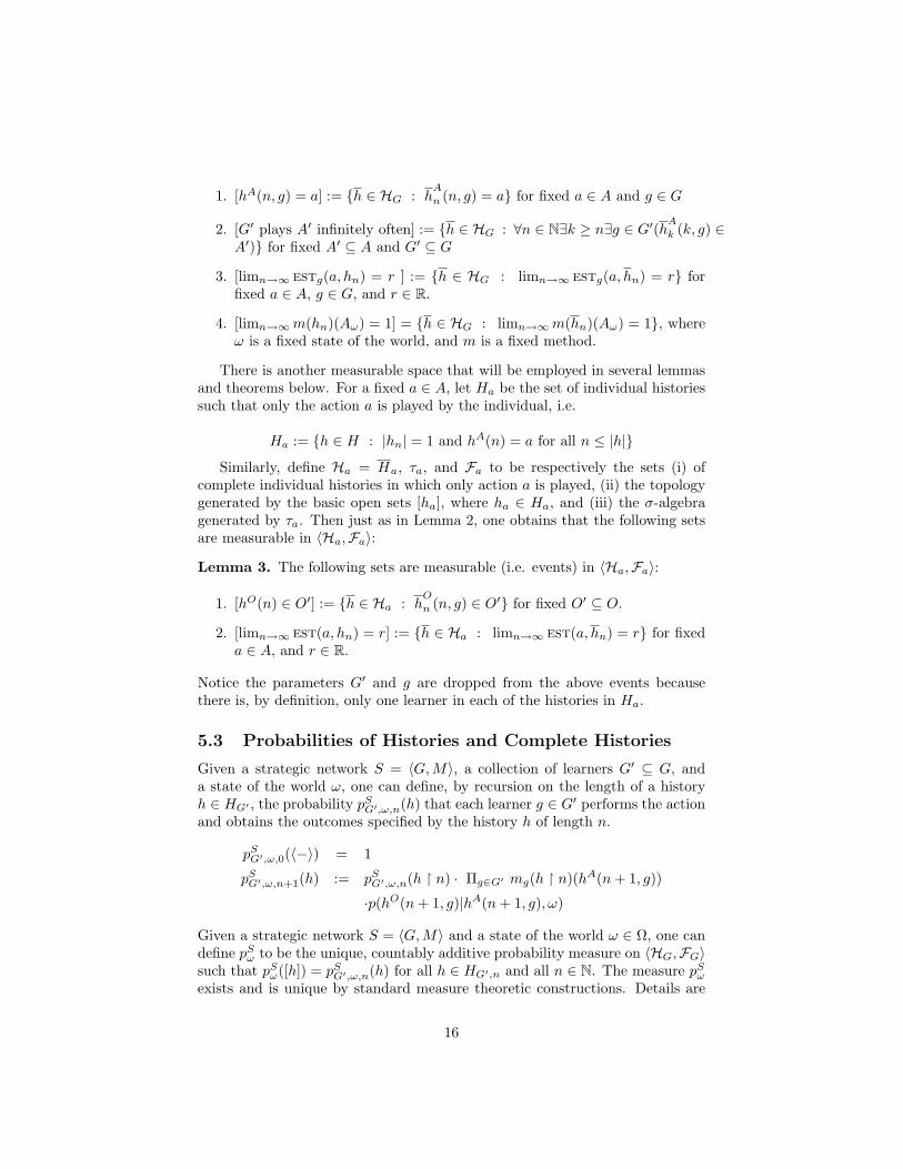
2. [G′ plays A′ infinitely often] := h ∈ HG : ∀n ∈ N∃k ≥ n∃g ∈ G′(hAk (k, g) ∈A′) for fixed A′ ⊆ A and G′ ⊆ G

3. [limn→∞ estg(a, hn) = r ] := h ∈ HG : limn→∞ estg(a, hn) = r forfixed a ∈ A, g ∈ G, and r ∈ R.

4. [limn→∞m(hn)(Aω) = 1] = h ∈ HG : limn→∞m(hn)(Aω) = 1, whereω is a fixed state of the world, and m is a fixed method.

There is another measurable space that will be employed in several lemmasand theorems below. For a fixed a ∈ A, let Ha be the set of individual historiessuch that only the action a is played by the individual, i.e.

Ha := h ∈ H : |hn| = 1 and hA(n) = a for all n ≤ |h|

Similarly, define Ha = Ha, τa, and Fa to be respectively the sets (i) ofcomplete individual histories in which only action a is played, (ii) the topologygenerated by the basic open sets [ha], where ha ∈ Ha, and (iii) the σ-algebragenerated by τa. Then just as in Lemma 2, one obtains that the following setsare measurable in 〈Ha,Fa〉:

Lemma 3. The following sets are measurable (i.e. events) in 〈Ha,Fa〉:

1. [hO(n) ∈ O′] := h ∈ Ha : hO

n (n, g) ∈ O′ for fixed O′ ⊆ O.

2. [limn→∞ est(a, hn) = r] := h ∈ Ha : limn→∞ est(a, hn) = r for fixeda ∈ A, and r ∈ R.

Notice the parameters G′ and g are dropped from the above events becausethere is, by definition, only one learner in each of the histories in Ha.

5.3 Probabilities of Histories and Complete Histories

Given a strategic network S = 〈G,M〉, a collection of learners G′ ⊆ G, anda state of the world ω, one can define, by recursion on the length of a historyh ∈ HG′ , the probability pSG′,ω,n(h) that each learner g ∈ G′ performs the actionand obtains the outcomes specified by the history h of length n.

pSG′,ω,0(〈−〉) = 1

pSG′,ω,n+1(h) := pSG′,ω,n(h n) · Πg∈G′ mg(h n)(hA(n+ 1, g))

·p(hO(n+ 1, g)|hA(n+ 1, g), ω)

Given a strategic network S = 〈G,M〉 and a state of the world ω ∈ Ω, one candefine pSω to be the unique, countably additive probability measure on 〈HG,FG〉such that pSω([h]) = pSG′,ω,n(h) for all h ∈ HG′,n and all n ∈ N. The measure pSωexists and is unique by standard measure theoretic constructions. Details are

16

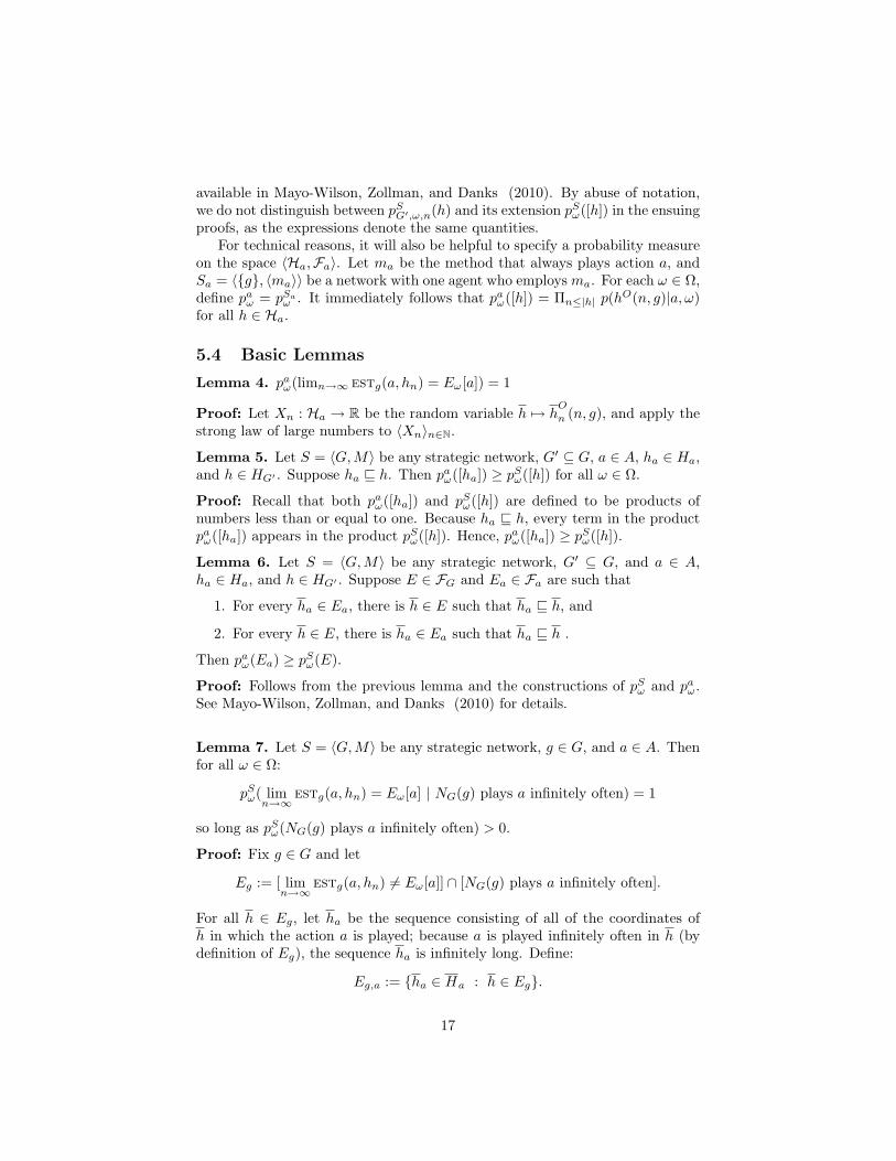
available in Mayo-Wilson, Zollman, and Danks (2010). By abuse of notation,we do not distinguish between pSG′,ω,n(h) and its extension pSω([h]) in the ensuingproofs, as the expressions denote the same quantities.

For technical reasons, it will also be helpful to specify a probability measureon the space 〈Ha,Fa〉. Let ma be the method that always plays action a, andSa = 〈g, 〈ma〉〉 be a network with one agent who employs ma. For each ω ∈ Ω,define paω = pSaω . It immediately follows that paω([h]) = Πn≤|h| p(hO(n, g)|a, ω)for all h ∈ Ha.

5.4 Basic Lemmas

Lemma 4. paω(limn→∞ estg(a, hn) = Eω[a]) = 1

Proof: Let Xn : Ha → R be the random variable h 7→ hO

n (n, g), and apply thestrong law of large numbers to 〈Xn〉n∈N.

Lemma 5. Let S = 〈G,M〉 be any strategic network, G′ ⊆ G, a ∈ A, ha ∈ Ha,and h ∈ HG′ . Suppose ha v h. Then paω([ha]) ≥ pSω([h]) for all ω ∈ Ω.

Proof: Recall that both paω([ha]) and pSω([h]) are defined to be products ofnumbers less than or equal to one. Because ha v h, every term in the productpaω([ha]) appears in the product pSω([h]). Hence, paω([ha]) ≥ pSω([h]).

Lemma 6. Let S = 〈G,M〉 be any strategic network, G′ ⊆ G, and a ∈ A,ha ∈ Ha, and h ∈ HG′ . Suppose E ∈ FG and Ea ∈ Fa are such that

1. For every ha ∈ Ea, there is h ∈ E such that ha v h, and

2. For every h ∈ E, there is ha ∈ Ea such that ha v h .

Then paω(Ea) ≥ pSω(E).

Proof: Follows from the previous lemma and the constructions of pSω and paω.See Mayo-Wilson, Zollman, and Danks (2010) for details.

Lemma 7. Let S = 〈G,M〉 be any strategic network, g ∈ G, and a ∈ A. Thenfor all ω ∈ Ω:

pSω( limn→∞

estg(a, hn) = Eω[a] | NG(g) plays a infinitely often) = 1

so long as pSω(NG(g) plays a infinitely often) > 0.

Proof: Fix g ∈ G and let

Eg := [ limn→∞

estg(a, hn) 6= Eω[a]] ∩ [NG(g) plays a infinitely often].

For all h ∈ Eg, let ha be the sequence consisting of all of the coordinates ofh in which the action a is played; because a is played infinitely often in h (bydefinition of Eg), the sequence ha is infinitely long. Define:

Eg,a := ha ∈ Ha : h ∈ Eg.

17

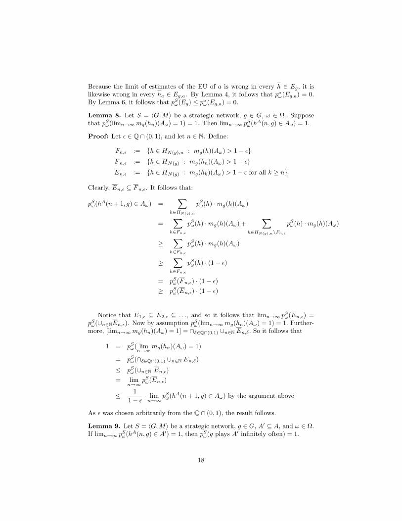
Because the limit of estimates of the EU of a is wrong in every h ∈ Eg, it islikewise wrong in every ha ∈ Eg,a. By Lemma 4, it follows that paω(Eg,a) = 0.By Lemma 6, it follows that pSω(Eg) ≤ paω(Eg,a) = 0.

Lemma 8. Let S = 〈G,M〉 be a strategic network, g ∈ G, ω ∈ Ω. Supposethat pSω(limn→∞mg(hn)(Aω) = 1) = 1. Then limn→∞ pSω(hA(n, g) ∈ Aω) = 1.

Proof: Let ε ∈ Q ∩ (0, 1), and let n ∈ N. Define:

Fn,ε := h ∈ HN(g),n : mg(h)(Aω) > 1− εFn,ε := h ∈ HN(g) : mg(hn)(Aω) > 1− εEn,ε := h ∈ HN(g) : mg(hk)(Aω) > 1− ε for all k ≥ n

Clearly, En,ε ⊆ Fn,ε. It follows that:

pSω(hA(n+ 1, g) ∈ Aω) =∑

h∈HN(g),n

pSω(h) ·mg(h)(Aω)

=∑

h∈Fn,ε

pSω(h) ·mg(h)(Aω) +∑

h∈HN(g),n\Fn,ε

pSω(h) ·mg(h)(Aω)

≥∑

h∈Fn,ε

pSω(h) ·mg(h)(Aω)

≥∑

h∈Fn,ε

pSω(h) · (1− ε)

= pSω(Fn,ε) · (1− ε)≥ pSω(En,ε) · (1− ε)

Notice that E1,ε ⊆ E2,ε ⊆ . . ., and so it follows that limn→∞ pSω(En,ε) =pSω(∪n∈NEn,ε). Now by assumption pSω(limn→∞mg(hn)(Aω) = 1) = 1. Further-more, [limn→∞mg(hn)(Aω) = 1] = ∩δ∈Q∩(0,1) ∪n∈N En,δ. So it follows that

1 = pSω( limn→∞

mg(hn)(Aω) = 1)

= pSω(∩δ∈Q∩(0,1) ∪n∈N En,δ)

≤ pSω(∪n∈N En,ε)= lim

n→∞pSω(En,ε)

≤ 11− ε

· limn→∞

pSω(hA(n+ 1, g) ∈ Aω) by the argument above

As ε was chosen arbitrarily from the Q ∩ (0, 1), the result follows.

Lemma 9. Let S = 〈G,M〉 be a strategic network, g ∈ G, A′ ⊆ A, and ω ∈ Ω.If limn→∞ pSω(hA(n, g) ∈ A′) = 1, then pSω(g plays A′ infinitely often) = 1.

18

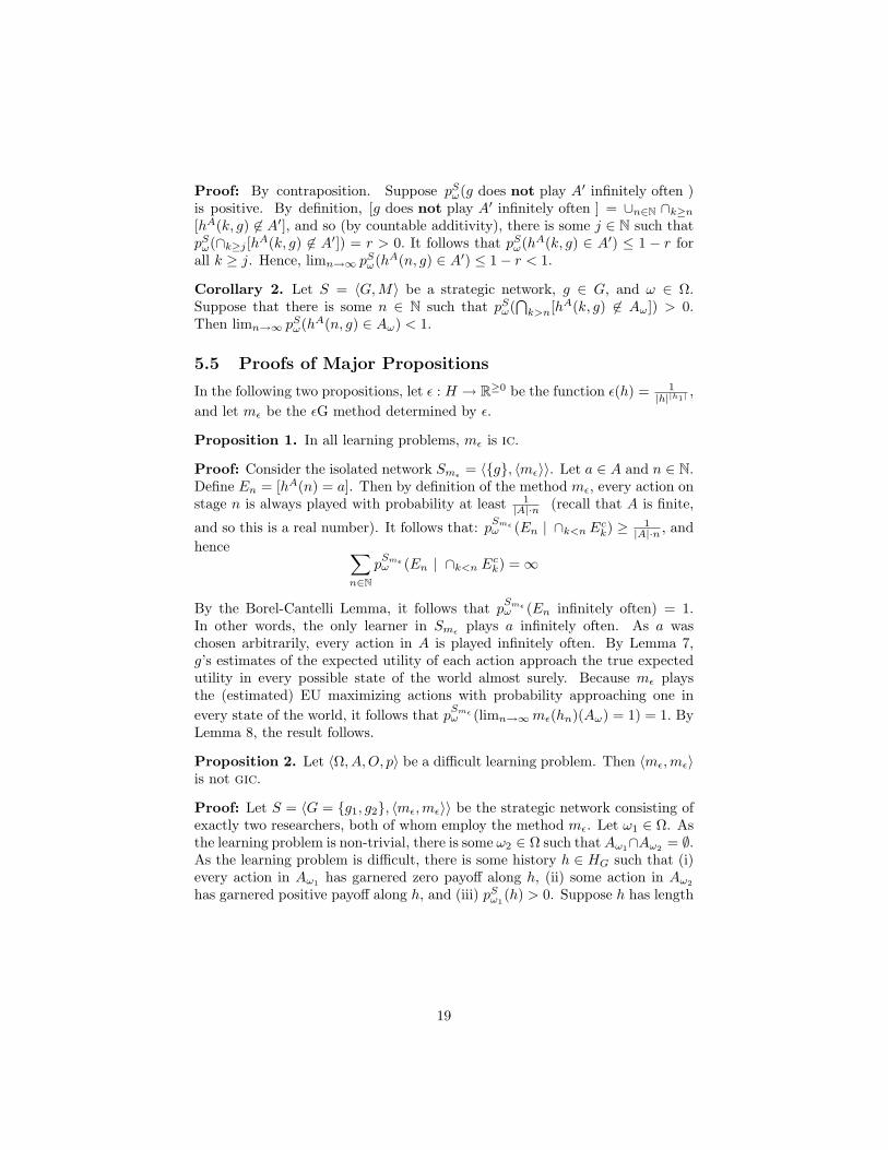
Proof: By contraposition. Suppose pSω(g does not play A′ infinitely often )is positive. By definition, [g does not play A′ infinitely often ] = ∪n∈N ∩k≥n[hA(k, g) 6∈ A′], and so (by countable additivity), there is some j ∈ N such thatpSω(∩k≥j [hA(k, g) 6∈ A′]) = r > 0. It follows that pSω(hA(k, g) ∈ A′) ≤ 1 − r forall k ≥ j. Hence, limn→∞ pSω(hA(n, g) ∈ A′) ≤ 1− r < 1.

Corollary 2. Let S = 〈G,M〉 be a strategic network, g ∈ G, and ω ∈ Ω.Suppose that there is some n ∈ N such that pSω(

⋂k>n[hA(k, g) 6∈ Aω]) > 0.

Then limn→∞ pSω(hA(n, g) ∈ Aω) < 1.

5.5 Proofs of Major Propositions

In the following two propositions, let ε : H → R≥0 be the function ε(h) = 1|h||h1| ,

and let mε be the εG method determined by ε.

Proposition 1. In all learning problems, mε is ic.

Proof: Consider the isolated network Smε = 〈g, 〈mε〉〉. Let a ∈ A and n ∈ N.Define En = [hA(n) = a]. Then by definition of the method mε, every action onstage n is always played with probability at least 1

|A|·n (recall that A is finite,

and so this is a real number). It follows that: pSmεω (En | ∩k<n Eck) ≥ 1|A|·n , and

hence ∑n∈N

pSmεω (En | ∩k<n Eck) =∞

By the Borel-Cantelli Lemma, it follows that pSmεω (En infinitely often) = 1.In other words, the only learner in Smε plays a infinitely often. As a waschosen arbitrarily, every action in A is played infinitely often. By Lemma 7,g’s estimates of the expected utility of each action approach the true expectedutility in every possible state of the world almost surely. Because mε playsthe (estimated) EU maximizing actions with probability approaching one inevery state of the world, it follows that pSmεω (limn→∞mε(hn)(Aω) = 1) = 1. ByLemma 8, the result follows.

Proposition 2. Let 〈Ω, A,O, p〉 be a difficult learning problem. Then 〈mε,mε〉is not gic.

Proof: Let S = 〈G = g1, g2, 〈mε,mε〉〉 be the strategic network consisting ofexactly two researchers, both of whom employ the method mε. Let ω1 ∈ Ω. Asthe learning problem is non-trivial, there is some ω2 ∈ Ω such that Aω1∩Aω2 = ∅.As the learning problem is difficult, there is some history h ∈ HG such that (i)every action in Aω1 has garnered zero payoff along h, (ii) some action in Aω2

has garnered positive payoff along h, and (iii) pSω1(h) > 0. Suppose h has length

19

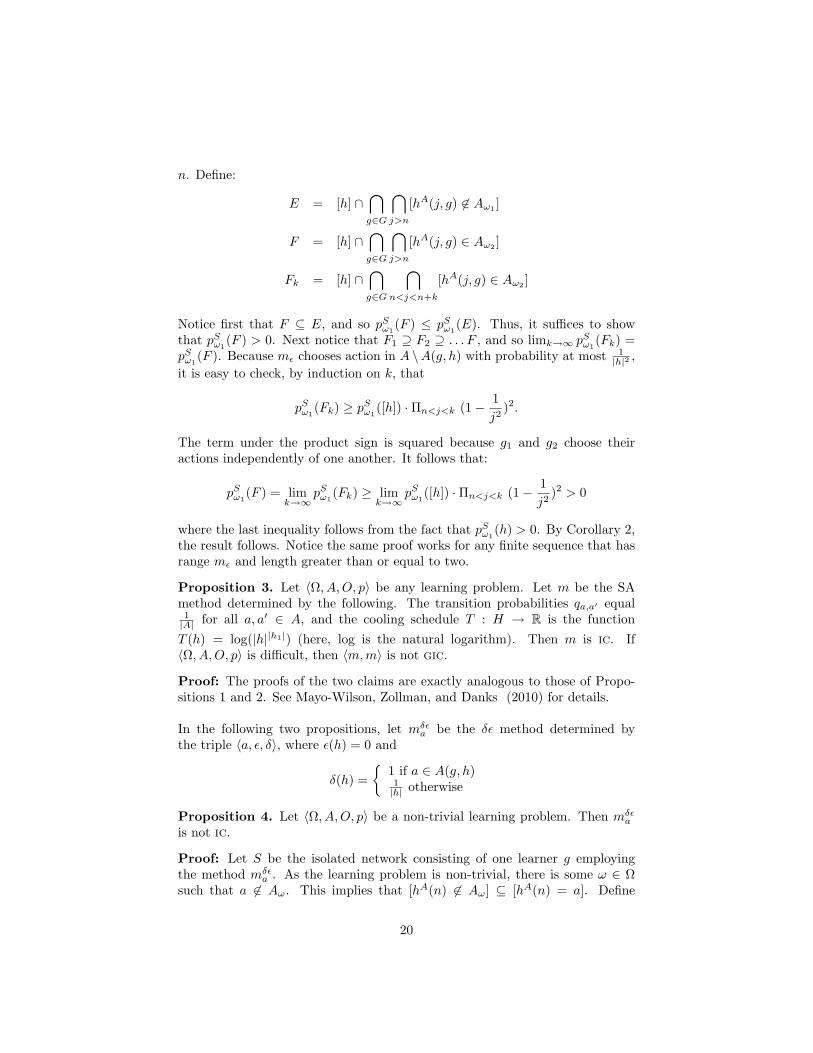
n. Define:

E = [h] ∩⋂g∈G

⋂j>n

[hA(j, g) 6∈ Aω1 ]

F = [h] ∩⋂g∈G

⋂j>n

[hA(j, g) ∈ Aω2 ]

Fk = [h] ∩⋂g∈G

⋂n<j<n+k

[hA(j, g) ∈ Aω2 ]

Notice first that F ⊆ E, and so pSω1(F ) ≤ pSω1

(E). Thus, it suffices to showthat pSω1

(F ) > 0. Next notice that F1 ⊇ F2 ⊇ . . . F , and so limk→∞ pSω1(Fk) =

pSω1(F ). Because mε chooses action in A \A(g, h) with probability at most 1

|h|2 ,it is easy to check, by induction on k, that

pSω1(Fk) ≥ pSω1

([h]) ·Πn<j<k (1− 1j2

)2.

The term under the product sign is squared because g1 and g2 choose theiractions independently of one another. It follows that:

pSω1(F ) = lim

k→∞pSω1

(Fk) ≥ limk→∞

pSω1([h]) ·Πn<j<k (1− 1

j2)2 > 0

where the last inequality follows from the fact that pSω1(h) > 0. By Corollary 2,

the result follows. Notice the same proof works for any finite sequence that hasrange mε and length greater than or equal to two.

Proposition 3. Let 〈Ω, A,O, p〉 be any learning problem. Let m be the SAmethod determined by the following. The transition probabilities qa,a′ equal1|A| for all a, a′ ∈ A, and the cooling schedule T : H → R is the functionT (h) = log(|h||h1|) (here, log is the natural logarithm). Then m is ic. If〈Ω, A,O, p〉 is difficult, then 〈m,m〉 is not gic.

Proof: The proofs of the two claims are exactly analogous to those of Propo-sitions 1 and 2. See Mayo-Wilson, Zollman, and Danks (2010) for details.

In the following two propositions, let mδεa be the δε method determined by

the triple 〈a, ε, δ〉, where ε(h) = 0 and

δ(h) =

1 if a ∈ A(g, h)1|h| otherwise

Proposition 4. Let 〈Ω, A,O, p〉 be a non-trivial learning problem. Then mδεa

is not ic.

Proof: Let S be the isolated network consisting of one learner g employingthe method mδε

a . As the learning problem is non-trivial, there is some ω ∈ Ωsuch that a 6∈ Aω. This implies that [hA(n) 6∈ Aω] ⊆ [hA(n) = a]. Define

20

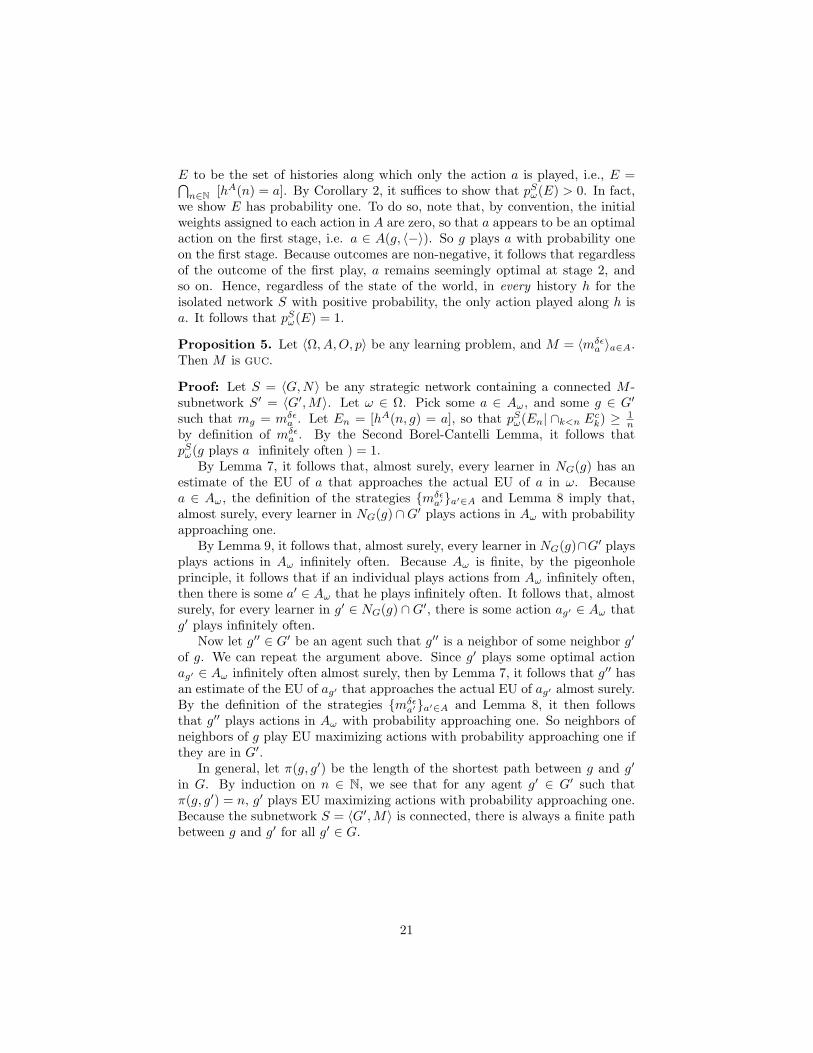
E to be the set of histories along which only the action a is played, i.e., E =⋂n∈N [hA(n) = a]. By Corollary 2, it suffices to show that pSω(E) > 0. In fact,

we show E has probability one. To do so, note that, by convention, the initialweights assigned to each action in A are zero, so that a appears to be an optimalaction on the first stage, i.e. a ∈ A(g, 〈−〉). So g plays a with probability oneon the first stage. Because outcomes are non-negative, it follows that regardlessof the outcome of the first play, a remains seemingly optimal at stage 2, andso on. Hence, regardless of the state of the world, in every history h for theisolated network S with positive probability, the only action played along h isa. It follows that pSω(E) = 1.

Proposition 5. Let 〈Ω, A,O, p〉 be any learning problem, and M = 〈mδεa 〉a∈A.

Then M is guc.

Proof: Let S = 〈G,N〉 be any strategic network containing a connected M -subnetwork S′ = 〈G′,M〉. Let ω ∈ Ω. Pick some a ∈ Aω, and some g ∈ G′

such that mg = mδεa . Let En = [hA(n, g) = a], so that pSω(En| ∩k<n Eck) ≥ 1

nby definition of mδε

a . By the Second Borel-Cantelli Lemma, it follows thatpSω(g plays a infinitely often ) = 1.

By Lemma 7, it follows that, almost surely, every learner in NG(g) has anestimate of the EU of a that approaches the actual EU of a in ω. Becausea ∈ Aω, the definition of the strategies mδε

a′a′∈A and Lemma 8 imply that,almost surely, every learner in NG(g) ∩G′ plays actions in Aω with probabilityapproaching one.

By Lemma 9, it follows that, almost surely, every learner in NG(g)∩G′ playsplays actions in Aω infinitely often. Because Aω is finite, by the pigeonholeprinciple, it follows that if an individual plays actions from Aω infinitely often,then there is some a′ ∈ Aω that he plays infinitely often. It follows that, almostsurely, for every learner in g′ ∈ NG(g) ∩G′, there is some action ag′ ∈ Aω thatg′ plays infinitely often.

Now let g′′ ∈ G′ be an agent such that g′′ is a neighbor of some neighbor g′

of g. We can repeat the argument above. Since g′ plays some optimal actionag′ ∈ Aω infinitely often almost surely, then by Lemma 7, it follows that g′′ hasan estimate of the EU of ag′ that approaches the actual EU of ag′ almost surely.By the definition of the strategies mδε

a′a′∈A and Lemma 8, it then followsthat g′′ plays actions in Aω with probability approaching one. So neighbors ofneighbors of g play EU maximizing actions with probability approaching one ifthey are in G′.

In general, let π(g, g′) be the length of the shortest path between g and g′

in G. By induction on n ∈ N, we see that for any agent g′ ∈ G′ such thatπ(g, g′) = n, g′ plays EU maximizing actions with probability approaching one.Because the subnetwork S = 〈G′,M〉 is connected, there is always a finite pathbetween g and g′ for all g′ ∈ G.

21

5.6 Proofs of Theorems

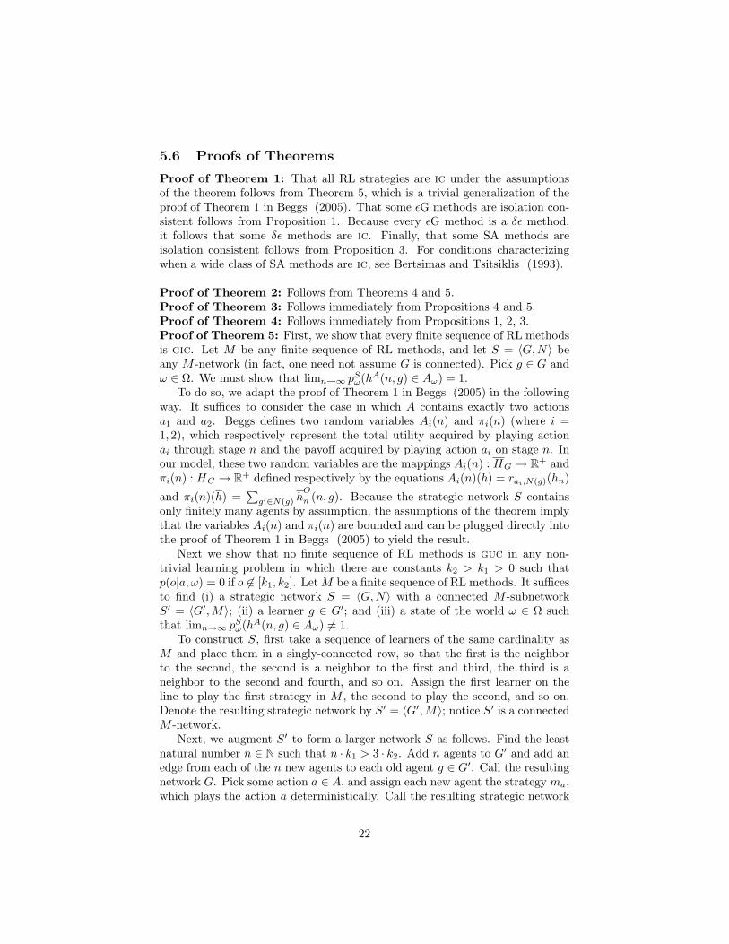
Proof of Theorem 1: That all RL strategies are ic under the assumptionsof the theorem follows from Theorem 5, which is a trivial generalization of theproof of Theorem 1 in Beggs (2005). That some εG methods are isolation con-sistent follows from Proposition 1. Because every εG method is a δε method,it follows that some δε methods are ic. Finally, that some SA methods areisolation consistent follows from Proposition 3. For conditions characterizingwhen a wide class of SA methods are ic, see Bertsimas and Tsitsiklis (1993).

Proof of Theorem 2: Follows from Theorems 4 and 5.Proof of Theorem 3: Follows immediately from Propositions 4 and 5.Proof of Theorem 4: Follows immediately from Propositions 1, 2, 3.Proof of Theorem 5: First, we show that every finite sequence of RL methodsis gic. Let M be any finite sequence of RL methods, and let S = 〈G,N〉 beany M -network (in fact, one need not assume G is connected). Pick g ∈ G andω ∈ Ω. We must show that limn→∞ pSω(hA(n, g) ∈ Aω) = 1.

To do so, we adapt the proof of Theorem 1 in Beggs (2005) in the followingway. It suffices to consider the case in which A contains exactly two actionsa1 and a2. Beggs defines two random variables Ai(n) and πi(n) (where i =1, 2), which respectively represent the total utility acquired by playing actionai through stage n and the payoff acquired by playing action ai on stage n. Inour model, these two random variables are the mappings Ai(n) : HG → R+ andπi(n) : HG → R+ defined respectively by the equations Ai(n)(h) = rai,N(g)(hn)

and πi(n)(h) =∑g′∈N(g) h

O

n (n, g). Because the strategic network S containsonly finitely many agents by assumption, the assumptions of the theorem implythat the variables Ai(n) and πi(n) are bounded and can be plugged directly intothe proof of Theorem 1 in Beggs (2005) to yield the result.

Next we show that no finite sequence of RL methods is guc in any non-trivial learning problem in which there are constants k2 > k1 > 0 such thatp(o|a, ω) = 0 if o 6∈ [k1, k2]. Let M be a finite sequence of RL methods. It sufficesto find (i) a strategic network S = 〈G,N〉 with a connected M -subnetworkS′ = 〈G′,M〉; (ii) a learner g ∈ G′; and (iii) a state of the world ω ∈ Ω suchthat limn→∞ pSω(hA(n, g) ∈ Aω) 6= 1.

To construct S, first take a sequence of learners of the same cardinality asM and place them in a singly-connected row, so that the first is the neighborto the second, the second is a neighbor to the first and third, the third is aneighbor to the second and fourth, and so on. Assign the first learner on theline to play the first strategy in M , the second to play the second, and so on.Denote the resulting strategic network by S′ = 〈G′,M〉; notice S′ is a connectedM -network.

Next, we augment S′ to form a larger network S as follows. Find the leastnatural number n ∈ N such that n · k1 > 3 · k2. Add n agents to G′ and add anedge from each of the n new agents to each old agent g ∈ G′. Call the resultingnetwork G. Pick some action a ∈ A, and assign each new agent the strategy ma,which plays the action a deterministically. Call the resulting strategic network

22

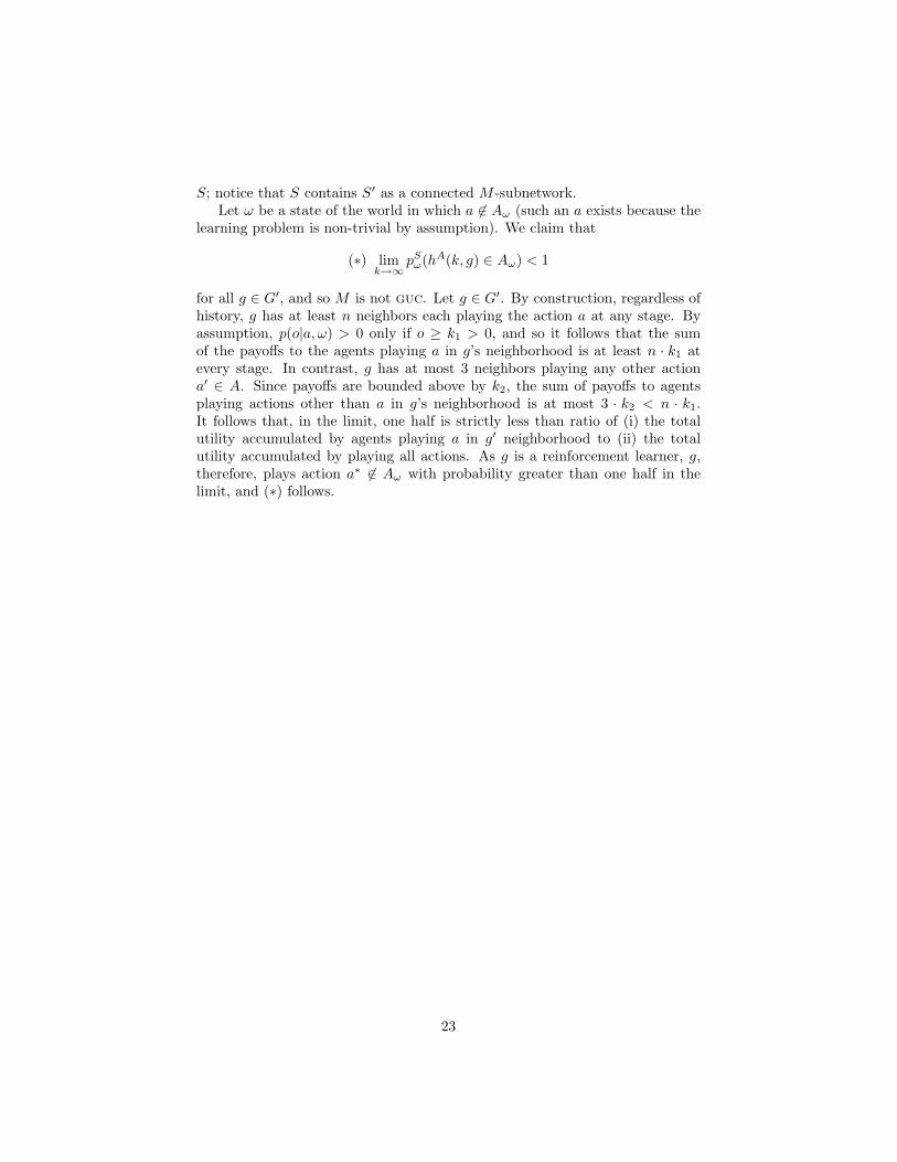
S; notice that S contains S′ as a connected M -subnetwork.Let ω be a state of the world in which a 6∈ Aω (such an a exists because the

learning problem is non-trivial by assumption). We claim that

(∗) limk→∞

pSω(hA(k, g) ∈ Aω) < 1

for all g ∈ G′, and so M is not guc. Let g ∈ G′. By construction, regardless ofhistory, g has at least n neighbors each playing the action a at any stage. Byassumption, p(o|a, ω) > 0 only if o ≥ k1 > 0, and so it follows that the sumof the payoffs to the agents playing a in g’s neighborhood is at least n · k1 atevery stage. In contrast, g has at most 3 neighbors playing any other actiona′ ∈ A. Since payoffs are bounded above by k2, the sum of payoffs to agentsplaying actions other than a in g’s neighborhood is at most 3 · k2 < n · k1.It follows that, in the limit, one half is strictly less than ratio of (i) the totalutility accumulated by agents playing a in g′ neighborhood to (ii) the totalutility accumulated by playing all actions. As g is a reinforcement learner, g,therefore, plays action a∗ 6∈ Aω with probability greater than one half in thelimit, and (∗) follows.

23