Why the Sudden Change? - Tufts University · Why the Sudden Change? ... Landsat 5 and Landsat 8...
1
Why the Sudden Change? A search into the causes for the expansion of dengue fever outbreaks into previously unaffected areas. Jody Kenworthy Dengue Fever vectors, the A edes aegypti mosquito, until recently, have usually been found at altitudes below 1,600 meters. Over 700 Aedes aegypti mosquito abundance data points were collected in July and August of 2011 and 2012, at altitudes between 9 meters below sea level to 2,472 meters above sea level, between Mexico City, and Vera- cruz, Mexico to study the reasons behind the mosquito’s adaptation to new and different environments, see Figure 1. The highest altitude recorded, within these data points, is over 800 meters above 1,600 me- ters. This analysis studies possible factors that have caused the expan- sion of the A edes aegypti mosquito to higher altitudes. It looks at Landsat 5 and 8 imagery, of the area around clusters of data points, in August of 2009 and 2013. And, uses supervised classi- fication methods Mahalanobis Distance, Minimum Distance, and Maximum Likelihood to categorize 8 classes for the 2009 data and 9 classes for the 2013 data. Finally, it uses change detection between 2009 and 2013 for each classification method to determine the land use change at the data points’ sites, between the four-year period. According to the Center for Disease Control (CDC), dengue fever is an endemic in over 100 countries, with 50-100 million infections each year, and 40 percent of the entire world population living in areas where the risk of infection exists. 1 The mosquitos are found in tropi- cal and subtropical climates and in urban areas. 2 Both natural and hu- man factors contribute to the spread of this disease, including the in- crease in the amount of area that is suitable for the mosquitos to breed. Natural factors include an increase in precipitation, average tempera- tures, and humidity. The human factors include deforestation, or changes in land use, and open water containers, including water bar- rels, wells, tires, and reservoirs, that are ideal breeding grounds for the Aedes aegypti mosquito. Landsat 5 and Landsat 8 images from the WRS 2 path 25 and WRS 2 row 47 were obtained from http://earthexplorer.usgs.gov/, to use in this analysis. As well as the 2005 North American MODIS Land Cover Data layer from http://landcover.usgs.gov/nalcms.php; this layer was used as a reference when creating training sites (regions-of-interest (ROIs)) for each class. All layers were then uploaded into ENVI and the individual bands for each year were stacked, using the Layer Stack tool, and a metadata header file was edited to add the wavelengths for each band and the date the image was acquired. Stacking the individu- al bands under one layer allowed the analysis to look at the change be- tween all bands at the same time. Figure 3 shows the 2005 Land Cover layer, and Figure 2 shows the 2009 and 2013 base images. Each classification method was good at measuring some type of land cover. The Minimum Distance method was good at measuring vegeta- tion and soil change. The Maximum Likelihood method was good at measuring urban/developed land change. The Mahalanobis Distance method was good at measuring both vegetation and urban change. The Maximum Likelihood and Mahalanobis Distance methods were the most accurate at classifying the training sites (ROIs). Table 1 shows the overall accuracy, as a percent, and the Kappa coefficient of each classification method for both 2009 and 2013. These accuracy num- bers were obtained from Confusions Matrices run on each method, us- ing different training sites (ROIs) in each year. Observing the change between land cover types between 2009 and 2013 is a good start to studying why locations that were previously un- suitable breeding sites for A edes aegypti mosquitos have become suita- ble. Further analysis should be performed and other factors should be considered to produce concrete results as what changes correlate to the expansion in land area mosquito breeding site suitably. In terms of this analysis, other training sites (ROIs), of the same classes, should be created, multiple times, and each classification method should be many times, changing the parameters, to locate overall trends in land cover change at each site. Introduction Figure 1: Area of Study Methodology Conclusion Figure 2: Base Maps 2009 Figure 2: 2005 Land Cover Data Figure 4: Mahalanobis Distance Figure 6: Minimum Distance Figure 5: Maximum Likelihood Figure 7: EVI Figure 8: Site 1 Results 2009 Legend 2013 2013 Before classifying the different land cover types, the different im- ages had to be coregistered using tie points with less than .3 error. A shapefile of the 700+ data points was created and uploaded into ENVI to use as a reference in creating a polygon around the points that laid within the image. This polygon was then used to create a mask of the area that the data points were in; the cloud coverage layer was also up- loaded and a mask was created to mask out the clouds. The masked- out data was set to equal “not-a-number” (NaN), so that those pixels were not considered during the classification and change detection pro- cesses. Eight classes were created for the 2009 data, and 9 classes for the 2013 data; these classes included Exposed Soil, Cropland, Shrubland, Urban, Forest, Water, Water Vegetation, and Lagoon (or shallow water/ wet soil). The additional ROI for the 2013 image was of Sub Polar land; this area of the 2009 image was masked by clouds, making it so no Sub Polar land pixels were visible to assign. Three supervised clas- sification methods, Minimum Distance, Mahalanobis Distance, and Maximum Likelihood, were used to compare the different types of land cover around the data points. Figures 4, 5, and 6 show the results for these three methods for 2009 and 2013. Table 1: Overall Accuracy of Classification Methods 2009 2013 2009 2013 Polygons were created around the data points to limit the amount of area observed to sixteen sites to be smaller and easier to analyze than the total images’ areas. Change detection was then run for each classi- fication method between 2009 and 2013. A mask of the sixteen sites was uploaded over the results for final analysis of each site. An En- hanced Vegetation Index (EVI) was also run for each year. An En- hanced Vegetation Index (EVI) displays the abundance of vegetation in an image. 3-4 Figure 7 shows the EVI results for 2009 and 2013, and Figure 8 shows the results for Site 1, of 16, for all processes. 2009 2013 Cartographer: Jody Kenworthy Class: CEE 194A; Instructor: Magaly Koch Projection: UTM WGS North America Zone N14 Data Sources: -Landsat 5 surface reflectance, cloud cover, and brightness temperature data for 1993, 1998, and 2009. http://earthexplorer.usgs.gov/ -Landsat 8 surface reflectance, cloud cover, and brightness temperature data for pro- jection for 2013. http://earthexplorer.usgs.gov/ -2005 North American Land Cover layer from USGS, using MODIS data. http:// landcover.usgs.gov/nalcms.php -Mexican State boundaries. ARCGIS. http://www.arcgis.com/home/item.html? id=ac9041c51b5c49c683fbfec61dc03ba8 -Latitude and longitude points used to collect mosquito data References: 1. Centers for Disease Control and Prevention (CDC). Dengue Homepage. Epi- demiology. Visited on 4/29/16. http://www.cdc.gov/dengue/epidemiology/ index.html#global 2. Project diagram designed by : Lee Gehrke, Irene Bosch and Magaly Koch (MIT) and Carlos Welch-Rodriguez (Mexico). Understanding optimal condi- tions for mosquito abundance using satellite remote sensing environmental monitoring and predictive correlation modeling in Veracruz, Mexico 3. Waring, R.H., Coops, N.C., Fan, E., and Nightingale, J.M. (2006) MODIS en- hanced vegetation index predicts tree species richness across forested ecore- gions in the contiguous U.S.A. Remote Sensing of Environment. 103. 218- 226 4. Jiang, Z., Huete, A.R., Didan, K., and Miura, T. (2008) Development of a two -band enhanced vegetation index without a blue band. Remote Sensing of En- vironment. 112. 3833-3845 Year Classificaon Method Overall Accuracy Kappa Coefficient 2009 Mahalanobis Distance 97.4% .9665 Maximum Likelihood 94.2% .9258 Minimum Distance 79.0% .7391 2013 Mahalanobis Distance 88.7% .8648 Maximum Likelihood 89.7% .8802 Minimum Distance 73.5% .6906
Transcript of Why the Sudden Change? - Tufts University · Why the Sudden Change? ... Landsat 5 and Landsat 8...
Why the Sudden Change? A search into the causes for the expansion of dengue fever outbreaks into previously
unaffected areas.
Jody Kenworthy
Dengue Fever vectors, the Aedes aegypti mosquito, until recently,
have usually been found at altitudes below 1,600 meters. Over 700
Aedes aegypti mosquito abundance data points were collected in July
and August of 2011 and 2012, at altitudes between 9 meters below sea
level to 2,472 meters above sea level, between Mexico City, and Vera-
cruz, Mexico to study the reasons behind the mosquito’s adaptation to
new and different environments, see Figure 1. The highest altitude
recorded, within these data points, is over 800 meters above 1,600 me-
ters. This analysis studies possible factors that have caused the expan-
sion of the Aedes aegypti mosquito to higher altitudes.
It looks at Landsat 5 and 8 imagery, of the area around clusters of
data points, in August of 2009 and 2013. And, uses supervised classi-
fication methods Mahalanobis Distance, Minimum Distance, and
Maximum Likelihood to categorize 8 classes for the 2009 data and 9
classes for the 2013 data. Finally, it uses change detection between
2009 and 2013 for each classification method to determine the land
use change at the data points’ sites, between the four-year period.
According to the Center for Disease Control (CDC), dengue fever
is an endemic in over 100 countries, with 50-100 million infections
each year, and 40 percent of the entire world population living in areas
where the risk of infection exists.1 The mosquitos are found in tropi-
cal and subtropical climates and in urban areas.2 Both natural and hu-
man factors contribute to the spread of this disease, including the in-
crease in the amount of area that is suitable for the mosquitos to breed.
Natural factors include an increase in precipitation, average tempera-
tures, and humidity. The human factors include deforestation, or
changes in land use, and open water containers, including water bar-
rels, wells, tires, and reservoirs, that are ideal breeding grounds for the
Aedes aegypti mosquito.
Landsat 5 and Landsat 8 images from the WRS 2 path 25 and WRS 2
row 47 were obtained from http://earthexplorer.usgs.gov/, to use in this
analysis. As well as the 2005 North American MODIS Land Cover
Data layer from http://landcover.usgs.gov/nalcms.php; this layer was
used as a reference when creating training sites (regions-of-interest
(ROIs)) for each class. All layers were then uploaded into ENVI and
the individual bands for each year were stacked, using the Layer Stack
tool, and a metadata header file was edited to add the wavelengths for
each band and the date the image was acquired. Stacking the individu-
al bands under one layer allowed the analysis to look at the change be-
tween all bands at the same time. Figure 3 shows the 2005 Land Cover
layer, and Figure 2 shows the 2009 and 2013 base images.
Each classification method was good at measuring some type of land
cover. The Minimum Distance method was good at measuring vegeta-
tion and soil change. The Maximum Likelihood method was good at
measuring urban/developed land change. The Mahalanobis Distance
method was good at measuring both vegetation and urban change. The
Maximum Likelihood and Mahalanobis Distance methods were the
most accurate at classifying the training sites (ROIs). Table 1 shows
the overall accuracy, as a percent, and the Kappa coefficient of each
classification method for both 2009 and 2013. These accuracy num-
bers were obtained from Confusions Matrices run on each method, us-
ing different training sites (ROIs) in each year.
Observing the change between land cover types between 2009 and
2013 is a good start to studying why locations that were previously un-
suitable breeding sites for Aedes aegypti mosquitos have become suita-
ble. Further analysis should be performed and other factors should be
considered to produce concrete results as what changes correlate to the
expansion in land area mosquito breeding site suitably. In terms of this analysis, other training sites (ROIs), of the
same classes, should be created, multiple
times, and each classification method should
be many times, changing the parameters, to
locate overall trends in land cover change at
each site.
Introduction
Figure 1: Area of Study
Methodology
Conclusion
Figure 2: Base Maps
2009
Figure 2: 2005 Land Cover Data
Figure 4: Mahalanobis Distance
Figure 6: Minimum Distance
Figure 5: Maximum Likelihood
Figure 7: EVI
Figure 8: Site 1 Results
2009
Legend
2013
2013
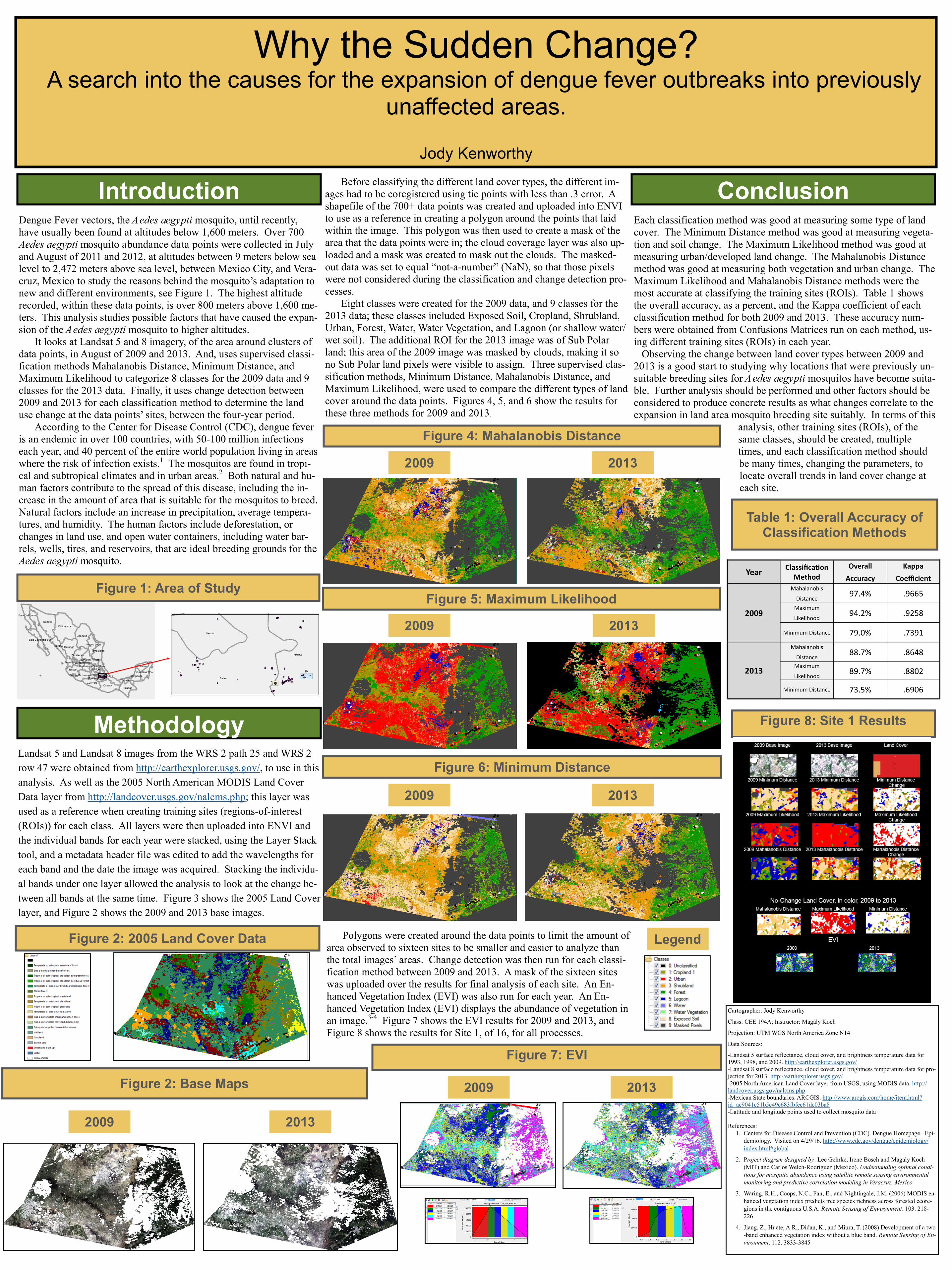
Before classifying the different land cover types, the different im-
ages had to be coregistered using tie points with less than .3 error. A
shapefile of the 700+ data points was created and uploaded into ENVI
to use as a reference in creating a polygon around the points that laid
within the image. This polygon was then used to create a mask of the
area that the data points were in; the cloud coverage layer was also up-
loaded and a mask was created to mask out the clouds. The masked-
out data was set to equal “not-a-number” (NaN), so that those pixels
were not considered during the classification and change detection pro-
cesses.
Eight classes were created for the 2009 data, and 9 classes for the
2013 data; these classes included Exposed Soil, Cropland, Shrubland,
Urban, Forest, Water, Water Vegetation, and Lagoon (or shallow water/
wet soil). The additional ROI for the 2013 image was of Sub Polar
land; this area of the 2009 image was masked by clouds, making it so
no Sub Polar land pixels were visible to assign. Three supervised clas-
sification methods, Minimum Distance, Mahalanobis Distance, and
Maximum Likelihood, were used to compare the different types of land
cover around the data points. Figures 4, 5, and 6 show the results for
these three methods for 2009 and 2013.
Table 1: Overall Accuracy of Classification Methods
2009 2013
2009 2013
Polygons were created around the data points to limit the amount of
area observed to sixteen sites to be smaller and easier to analyze than
the total images’ areas. Change detection was then run for each classi-
fication method between 2009 and 2013. A mask of the sixteen sites
was uploaded over the results for final analysis of each site. An En-
hanced Vegetation Index (EVI) was also run for each year. An En-
hanced Vegetation Index (EVI) displays the abundance of vegetation in
an image.3-4 Figure 7 shows the EVI results for 2009 and 2013, and
Figure 8 shows the results for Site 1, of 16, for all processes.
2009 2013
Cartographer: Jody Kenworthy
Class: CEE 194A; Instructor: Magaly Koch
Projection: UTM WGS North America Zone N14
Data Sources:
-Landsat 5 surface reflectance, cloud cover, and brightness temperature data for
1993, 1998, and 2009. http://earthexplorer.usgs.gov/
-Landsat 8 surface reflectance, cloud cover, and brightness temperature data for pro-
jection for 2013. http://earthexplorer.usgs.gov/
-2005 North American Land Cover layer from USGS, using MODIS data. http://
landcover.usgs.gov/nalcms.php
-Mexican State boundaries. ARCGIS. http://www.arcgis.com/home/item.html?
id=ac9041c51b5c49c683fbfec61dc03ba8
-Latitude and longitude points used to collect mosquito data
References:
1. Centers for Disease Control and Prevention (CDC). Dengue Homepage. Epi-
demiology. Visited on 4/29/16. http://www.cdc.gov/dengue/epidemiology/
index.html#global
2. Project diagram designed by: Lee Gehrke, Irene Bosch and Magaly Koch
(MIT) and Carlos Welch-Rodriguez (Mexico). Understanding optimal condi-
tions for mosquito abundance using satellite remote sensing environmental
monitoring and predictive correlation modeling in Veracruz, Mexico
3. Waring, R.H., Coops, N.C., Fan, E., and Nightingale, J.M. (2006) MODIS en-
hanced vegetation index predicts tree species richness across forested ecore-
gions in the contiguous U.S.A. Remote Sensing of Environment. 103. 218-
226
4. Jiang, Z., Huete, A.R., Didan, K., and Miura, T. (2008) Development of a two
-band enhanced vegetation index without a blue band. Remote Sensing of En-
vironment. 112. 3833-3845
Year Classification
Method
Overall
Accuracy
Kappa
Coefficient
2009
Mahalanobis
Distance 97.4% .9665
Maximum
Likelihood 94.2% .9258
Minimum Distance 79.0% .7391
2013
Mahalanobis
Distance 88.7% .8648
Maximum
Likelihood 89.7% .8802
Minimum Distance 73.5% .6906