Andreas Groll & Thomas Kneib & Andreas Mayr & GuntherSchauberger

Who’s the Favourite? – A Bivariate Poisson Modelfor the UEFA European Football Championship 2016

Technical Report Number 195, 2016Department of StatisticsUniversity of Munich

http://www.stat.uni-muenchen.de

Who’s the Favourite? – A Bivariate Poisson Model for the UEFA

European Football Championship 2016

A. Groll ∗ T. Kneib † A. Mayr ‡ G. Schauberger §

July 22, 2016

Abstract Many approaches that analyze and predict the results of soccer matches are based on two independentpairwise Poisson distributions. The dependence between the scores of two competing teams is simply displayedby the inclusion of the covariate information of both teams. One objective of this article is to analyze if thistype of modeling is appropriate or if an additional explicit modeling of the dependence structure for the jointscore of a soccer match needs to be taken into account. Therefore, a specific bivariate Poisson model for thetwo numbers of goals scored by national teams competing in UEFA European football championship matches isfitted to all matches from the three previous European championships, including covariate information of bothcompeting teams. A boosting approach is then used to select the relevant covariates. Based on the estimates, thecurrent tournament is simulated 1,000,000 times to obtain winning probabilities for all participating national teams.

Keywords Football, EURO 2016, Bivariate Poisson Model, Boosting, Variable selection.

1 Introduction

Many approaches that analyze and predict the results of soccer matches are based on two independent Poissondistributions. Both numbers of goals scored in single soccer matches are modeled seperately, assuming that eachscore follows its own Poisson distribution, see, e.g., Lee (1997) or Dyte and Clarke (2000). For example, Dyteand Clarke (2000) predict the distribution of scores in international soccer matches, treating each team’s goalsas conditionally independent Poisson variables depending on two influence variables, the FIFA ranking of eachteam and the match venue. Poisson regression is used to estimate parameters for the model and based on theseparameters the matches played during the 1998 FIFA World Cup were simulated.

However, it is well-known that the scores of two competing teams in a soccer match are correlated. One of the firstworks investigating the topic of dependency between scores of competing soccer teams is the fundamental article ofDixon and Coles (1997). There it has been shown that the joint distribution of the scores of both teams cannot bewell represented by the product of two independent marginal Poisson distributions of the home and away teams.They suggest to use an additional term to adjust for certain under- and overrepresented match results. Along theselines, Rue and Salvesen (2000) propose a similarly adjusted Poisson model with some additional modifications.After all, the findings in Dixon and Coles (1997) are based on the marginal distributions and only hold for modelswhere the predictors of both scores are uncorrelated. However, the model proposed by Dixon and Coles (1997)includes team-specific attack and defense ability parameters and then uses independent Poisson distributions forthe numbers of goals scored. Therefore, the linear predictor for the number of goals of a specific team depends bothon parameters of the team itself and its competitor. Groll et al. (2015) pointed out that when fitting exactly thesame model to FIFA World Cup data the estimates of the attack and defense abilities of the teams are negativelycorrelated. Therefore, although independent Poisson distributions are used for the scores in one match, the linearpredictors and, accordingly, the predicted outcomes are (negatively) correlated.

∗Department of Statistics, Ludwig-Maximilians-University Munich, Akademiestr. 1, 80799 Munich, Germany, andreas.groll@stat.uni-muenchen.de†Department of Statistics and Econometrics, Georg-August-University Goettingen, Humboldtallee 3, 37073 Goettingen, Germany,

tkneib@uni-goettingen.de‡IMBE, Friedrich-Alexander-University Erlangen-Nuernberg, Waldstrasse 6, 91054 Erlangen, Germany, andreas.mayr@fau.de§Department of Statistics, Ludwig-Maximilians-University Munich, Akademiestr. 1, 80799 Munich, Germany, gunther@stat.uni-

muenchen.de

1

These findings already indicate that up to a certain amount the dependence between the scores of two competingteams can simply be displayed by the inclusion of the covariate information of both teams. For example, Grolland Abedieh (2013) use a pairwise (independent) Poisson model for the number of goals scored by national teamsin the single matches of the UEFA European football championship (EURO), but incorporate several potentialinfluence variables of both competing teams in the linear predictors of the single Poisson distributions togetherwith additional team-specific random effects. Furthermore, in order to additionally account for the matched-pairdesign, they include a second match-specific random intercept, following Carlin et al. (2005), which is assumed to beindependent from the team-specific random intercept. However, it turns out that this additional random interceptis very small (< 1 · 10−5) and, hence, can be ignored. This provides further evidence that if highly informativecovariates of both competing teams are included into the linear predictor structure of both independent Poissondistributions, this might already appropriately model the dependence structure of the match scores.

These results are further confirmed in Groll et al. (2015). Following Groll and Abedieh (2013), an L1-regularizedindependent Poisson model is used on FIFA World Cup data. There, the linear predictors of the single independentPoisson components include, in addition to team-specific attack and defense abilities, the differences of severalcovariates of both competing teams. In an extensive goodness-of-fit analysis it is investigated if the obtaineddependence structure between the linear predictors of the two scores of a match represents the actual correlationsin an appropriate manner. For this purpose the correlations between the real outcomes and the model predictionsare compared and it turned out that the correlations within the linear predictors for both teams competing in amatch fully accounted for the correlation between the scores of those teams and that there was no need for furtheradjustment. So one major objective of this article is to analyze if this type of modeling is appropriate or if anadditional explicit modeling of the dependence structure for the joint score of a soccer match needs to be taken intoaccount.

One possibility to explicitly model (positive) dependence within the Poisson framework is the bivariate Poissondistribution. One of the first works dealing with this distribution in the context of soccer data is Maher (1982).An extensive study for the use of the bivariate Poisson distribution for the modeling of soccer data is found inKarlis and Ntzoufras (2003). There, the three parameters λ1, λ2 and λ3 of the bivariate Poisson distribution aremodeled by linear predictors depending on team-specific attack and defense abilities as well as team-specific homeeffect parameters. In particular, it is illustrated how also the third parameter λ3, which represents the covariancebetween the two scores, can be explicitly structured in terms of covariate effects (here: simply team-specific homeeffects). We adopt this approach in the present work and extend the linear predictors of the three parameters λ1,λ2 and λ3 of the bivariate Poisson distribution to include several covariate effects. We set up a specific bivariatePoisson model for the two numbers of goals scored by national teams competing in EURO tournaments includingcovariate information of both competing teams.

Note that in addition to the bivariate Poisson, also alternative approaches to handle the correlation of soccermatches have been proposed in the literature. For example, McHale and Scarf (2006, 2011) model the dependenceby using bivariate discrete distributions and by specifying a suitable family of dependence copulas.

A second objective of this work is to provide predictions of the current EURO 2016. Therefore, the proposedspecific bivariate Poisson model is fitted to all matches from the three previous EUROs 2004 - 2012, includingcovariate information of both competing teams. A suitable boosting approach is then used to select a small set ofrelevant covariates. Based on the obtained estimates, the current EURO 2016 tournament is simulated 1,000,000times to obtain winning probabilities for all participating national teams.

The rest of the article is structured as follows. In Section 2 we introduce the bivariate Poisson model for soccerdata. The boosting methodology for fitting the bivariate Poisson model for the number of goals is introduced inSection 2.4. Next, we present a list of several possible influence variables in Section 3.1 that will be considered inour regression analysis. Based on the boosting approach a selection of these covariates is determined yielding asparse model, which is then used in Section 4 for the prediction of the EURO 2016.

2 A Bivariate Poisson Model for Soccer Data

In the present section, we set up a specific bivariate Poisson model for the two numbers of goals scored by nationalteams competing in EURO tournaments including covariate information of both competing teams.

2

2.1 The Bivariate Poisson Distribution

In the following, we consider random variables Xk, k = 1, 2, 3, which follow independent Poisson distributions withparameters λk > 0. Then the random variables Y1 = X1 + X3 and Y2 = X2 + X3 follow a joint bivariate Poissondistribution, with a joint probability function

PY1,Y2(y1, y2) = P (Y1 = y1, Y2 = y2) (1)

= exp(−(λ1 + λ2 + λ3))λy11y1!

λy22y2!

min(y1,y2)∑

k=0

(y1k

)(y2k

)k!

(λ3λ1λ2

)k.

The bivariate Poisson distribution allows for dependence between the two random variables Y1 and Y2. Marginallyeach random variable follows a univariate Poisson distribution with E[Y1] = λ1+λ3 and E[Y2] = λ2+λ3. Moreover,the dependence of Y1 and Y2 is expressed by cov(Y1, Y2) = λ3. If λ3 = 0 holds, the two variables are independent andthe bivariate Poisson distribution reduces to the product of two independent Poisson distributions. The notationand usage of the bivariate Poisson distribution for modeling soccer data has been described in detail in Karlis andNtzoufras (2003).

2.2 Incorporation of Covariate Information

In general, each of the three parameters λk, k = 1, 2, 3, in the joint probability function (1) of the bivariate Poissondistribution can be modeled in terms of covariates by specifying a suitable response function, similar to classicalgeneralized linear models (GLMs). Hence, one could use, for example,

λk = exp(ηηηk) ,

with a linear predictor ηηηk = β0k + xTkβββk and response function h(·) = exp(·) in order to guarantee positive Poissonparameters λk. The vectors xk = (x1k, . . . , xpk)T collect all covariate information of predictor k.

2.3 Re-parametrization of the Bivariate Poisson Distribution

In the context of soccer data a natural way to model the three parameters λk, k = 1, 2, 3, would be to includethe covariate information of the competing teams 1 and 2 in λ1 and λ2, respectively, and some extra informationreflecting the match conditions of the corresponding match in λ3. However, the covariate effects βββk, k = 1, 2, usuallyshould be the same for both competing teams. Then, one obtains the model representation

λ1 = exp(β0 + xT1 βββ) , λ2 = exp(β0 + xT2 βββ) , (2)

with x1 and x2 denoting the covariates of team 1 and team 2. In contrast, the covariance parameter λ3 couldgenerally depend on different covariates and effects, i.e.

λ3 = exp(α0 + zTααα) , (3)

where z could contain parts of the covariates x1 and x2, or their differences or completely new covariates. If insteadin the linear predictors in (2) the differences of the teams’ covariates are used, one obtains

λ1 = exp(β0 + (x1 − x2)Tβββ) , λ2 = exp(β0 + (x2 − x1)Tβββ) ,

or, with x = x1 − x2, the simpler model

λk = exp(β0 ± xTβββ) , k = 1, 2 .

This allows to re-parametrize the bivariate Poisson probability function from (1) in the following way:

PY1,Y2(y1, y2) = P (Y1 = y1, Y2 = y2) (4)

= exp(−(γ1(γ2 + γ−12 ) + λ3))

(γ1γ2)y1

y1!

(γ1γ2 )y2

y2!

min(y1,y2)∑

k=0

(y1k

)(y2k

)k!

(λ3γ21

)k,

3

with λ1 = γ1γ2, λ2 = γ1γ2

. The new parameters γ1, γ2 are then given as functions of the following linear predictors:

γ1 = exp(β0) ,

γ2 = exp(xTβββ) ,

with x = x1 − x2 denoting the difference of both teams’ covariates.As before, we set λ3 = exp(α0 +zTααα). In the current analysis, we base the linear predictor of λ3 in general on the

same covariate differences. However, as we generally don’t want to prefer any specific direction of these differences,we use their absolute value and set λ3 = exp(α0 + |x|Tααα), where |x| = (|x11 − x21|, . . . , |x1p − x2p|)T .

2.4 Estimation

We apply a statistical boosting algorithm to estimate the linear predictors for γ1, γ2 and λ3. The concept ofboosting emerged from the field of machine learning (Freund and Schapire, 1996) and was later adapted to estimatepredictors for statistical models (Friedman et al., 2000; Friedman, 2001). Main advantages of statistical boostingalgorithms are their flexibility for high-dimensional data and their ability to incorporate variable selection in thefitting process (Mayr et al., 2014a). Furthermore, due to the modular nature of the algorithm, they are relativelyeasy to extend to new regression settings (Mayr et al., 2014b). The aim of the algorithm is to find estimates forthe predictors

exp(ηγ1) = exp(β0) = γ1 , (5)

exp(ηγ1) = exp(xT βββ) = γ2 , (6)

exp(ηλ3) = exp(α0 + |x|T ααα) = λ3 (7)

that optimize the multivariate likelihood of L(Y1, Y2, γ1, γ2, λ3) := PY1,Y2(y1, y2) with PY1,Y2(y1, y2) from Equa-tion (4), leading to the optimization problem

(ηγ1 , ηγ2 , ηλ3) = argmax(ηγ1 ,ηγ2 ,ηλ3 )

E [L(Y1, Y2, exp(ηγ1), exp(ηγ2), exp(ηλ3))] .

The algorithm cycles through the different predictors and carries out one boosting iteration for each. In everyboosting iteration, only one component of the corresponding predictor is selected to be updated, leading to auto-mated variable selection for the covariates. For more on boosting for multiple dimensions see Schmid et al. (2010)and Mayr et al. (2012). Let the data now be given by (y1i, y2i, x

Ti ), i = 1, . . . , n. Then, the following cyclic boosting

algorithm is applied:

(1) Initialize

Initialize the additive predictors with starting values, e.g. η[0]γ1 := log(y1); η

[0]γ2 := 0; η

[0]λ3

:= log(0.0001).Set iteration counter to m := 1.

(2) Boosting for γ1

Increase iteration counter: m := m+ 1

If m > mstopγ1 set η[m]γ1 := η

[m−1]γ1 and skip step (2).

Compute u[m] =(

∂∂ηγ1

L(y1i, y2i, exp(η[m−1]γ1 ), exp(η

[m−1]γ2 ), exp(η

[m−1]λ3

)))i=1,...,n

Estimate β0[m]

for u[m] by β0[m]

= u[m].

Update η[m]γ1 with β

[m]0 := β

[m−1]0 + ν · β[m]

0 , where ν is a small step length (e.g., ν = 0.1)

(3) Boosting for γ2

If m > mstopγ2 set η[m]γ2 := η

[m−1]γ2 and skip step (3).

4

Compute u[m] =(

∂∂ηγ2

L(y1i, y2i, exp(η[m]γ1 ), exp(η

[m−1]γ2 ), exp(η

[m−1]λ3

)))i=1,...,n

Fit all components of x separately to u[m], leading to β[m]1 , . . . , β

[m]p .

Select component j∗ that best fits u[m] with

j∗ = argmin1≤j≤p

n∑

i=1

(u[m]i − β[m]

j xj)2

Update η[m]γ2 with β

[m]j∗ = β

[m−1]j∗ + ν · β[m]

j∗ , keeping all other components fixed.

(4) Boosting for λ3

If m > mstopλ3set η

[m]λ3

:= η[m−1]λ3

and skip step (4).

Compute u[m] =(

∂∂ηγ2

L(y1i, y2i, exp(η[m]γ1 ), exp(η

[m]γ2 ), exp(η

[m−1]λ3

)))i=1,...,n

Fit all components of |x| separately to u[m], leading to α[m]0 , . . . , α

[m]p .

Select component j∗ that best fits u[m] with

j∗ = argmin0≤j≤p

n∑

i=1

(u[m]i − α[m]

j zj)2.

Update η[m]λ3

with α[m]j∗ = α

[m−1]j∗ + ν · α[m]

j∗ , keeping all other components fixed.

Iterate steps (2) to (4) until m ≥ max (mstopγ1 ,mstopγ2 ,mstopλ3)

Note that the presented algorithm reflects the structure for our re-parametrization of the bivariate Poissondistribution, but could also be easily adapted to estimate ηλk corresponding to the original parameters λk, k = 1, 2, 3.Furthermore, we focused on linear predictors in our approach, however, the algorithm’s structure stays the same ifnon-linear base-learners are applied to estimate additive predictors.

The main tuning parameters of the algorithm are the stopping iterations for the different predictors. They displaythe typical trade-off between small models with small variance and larger models with higher risk of overfitting.The best combination of stopping iterations (mstopγ1 ,mstopγ2 ,mstopλ3

) is typically chosen via cross-validation orresampling procedures or by optimizing the underlying likelihood on separate test data. The specification of thestep length ν is of minor importance as long as it is chosen small enough, it mainly affects the convergence speed(Schmid and Hothorn, 2008). The algorithm is implemented with the R add-on package gamboostLSS (Mayr et al.,2012; Hofner et al., 2016).

3 Application

In the following, the proposed model is applied to data from the previous EUROs 2004-2012 and is then used topredict the UEFA European championship 2016 in France.

3.1 Data

In this section a description of the covariates is given that are used (in the form of differences) in the bivariatePoisson regression model introduced in the previous sections. As most of these variables have already been used inGroll and Abedieh (2013) a more detailed description is found there. Several of the variables contain informationabout the recent performance and sportive success of national teams, as it is reasonable to assume that the currentform of a national team at the start of an European championship has an influence on the team’s success in thetournament, and thus on the goals the team will score. Besides these sportive variables, also economic factors,such as a country’s GDP and population size, are taken into account. Furthermore, variables are incorporatedthat describe the structure of a team’s squad. Note that several of these variables exhibit a substantial amountof correlation. The corresponding correlation matrix for all considered (differences of) covariates is presented inTable 5 in Appendix A.

5

Economic Factors:

• GDP1 per capita. The GDP per capita represents the economic power and welfare of a nation. Hence,countries with great prosperity might tend to focus more on sports training and promotion programs thanpoorer countries. The GDP per capita (in US Dollar) is publicly available on the website of The World Bank(see http://data.worldbank.org/indicator/NY.GDP.PCAP.CD).

• Population2. In general, larger countries have a deeper pool of talented soccer players from which a nationalcoach can recruit the national team squad. Hence, the population size might have an influence on the playingability of the corresponding national team. However, as this potential effect might not hold in a linearrelationship for arbitrarily large numbers of populations and instead might diminish (compare Bernard andBusse, 2004), the logarithm of the quantity is used.

Sportive Factors:

• Home advantage. There exist several studies that have analyzed the existence of a home advantage in soccer(see for example Pollard and Pollard, 2005; Pollard, 2008; Brown et al., 2002, for FIFA World Cups orClarke and Norman, 1995, for the English Premier league). Hence, there might also exist a home effect inEuropean championships. For this reason a dummy variable is used, indicating if a national team belongs tothe organizing countries.

• ODDSET odds. The analyses in Groll and Abedieh (2013) and Groll and Abedieh (2014) indicate thatbookmakers’ odds play an important role in the modeling of international soccer tournaments such as theEURO as they contain a lot of information with respect to the success of soccer teams. They include thebookmakers’ expertise and cover big parts of the team specific information and market appreciation withrespect to which teams are amongst the tournament’s favorites. For the EUROs from 2004 to 2012 the 16odds of all possible tournament winners before the start of the corresponding tournament have been obtainedfrom the German state betting agency ODDSET.

• Market value. The market value recently has gained increasing attention and importance in the context of pre-dicting the success of soccer teams (see, for example, Gerhards and Wagner, 2008, 2010; Gerhards et al., 2012,2014). Estimates of the teams’ average market values can be found on the webpage http://www.transfermarkt.de3.For each national team participating in a EURO these market value estimates (in Euro) have been collectedright before the start of the tournament.

• FIFA ranking. The FIFA ranking provides a ranking system for all national teams measuring the performanceof the teams over the last four years. The exact formula for the calculation of the underlying FIFA points andall rankings since implementation of the FIFA ranking system can be found at the official FIFA website (http://de.fifa.com/worldranking/index.html). Since the calculation formula of the FIFA points changed afterthe World Cup 2006, the rankings according to FIFA points are used instead of the points4.

• UEFA points. The associations’ club coefficients rankings are based on the results of each association’s clubsin the five previous UEFA CL and Europa League (previously UEFA Cup) seasons. The exact formula for thecalculation of the underlying UEFA points and all rankings since implementation of the UEFA ranking systemcan be found at the official UEFA website (http://www.uefa.com/memberassociations/uefarankings/country/index.html). The rankings determine the number of places allocated to an association (country)in the forthcoming UEFA club competitions. Thus, the UEFA points represent the strength and success ofa national league in comparison to other European national leagues. Besides, the more teams of a nationalleague participate in the UEFA CL and the UEFA Europa League, the more experience the players from that

1The GDP per capita is the gross domestic product divided by midyear population. The GDP is the sum of gross values added byall resident producers in the economy plus any product taxes and minus any subsidies not included in the value of the products.

2In order to collect data for all participating countries at the EURO 2004, 2008 and 2012, different sources had to be used. Amongstthe most useful ones are http://www.wko.at, http://www.statista.com/ and http://epp.eurostat.ec.europa.eu. For some years thepopulations of Russia and Ukraine had to be searched individually.

3Unfortunately, the archive of the webpage was established not until 4th October 2004, so the average market values of the nationalteams that we used for the EURO 2004 can only be seen as a rough approximation, as market values certainly changed after the EURO2004.

4The FIFA ranking was introduced in August 1993.

6

national league are able to earn on an international level. As usually a relationship between the level of anational league and the level of the national team of that country is supposed, the UEFA points could alsoaffect the performance of the corresponding national team.

Factors describing the team’s structure:

• (Second) maximum number of teammates5. If many players from one club play together in a national team,this could lead to an improved performance of the team as the teammates know each other better. Therefore,both the maximum and the second maximum number of teammates from the same club are counted andincluded as covariates.

• Average age. The average age of all 23 players is collected from the website http://www.transfermarkt.de

to include possible differences between rather old and rather young teams.

• Number of Champions League (Europa League) players5. The European club leagues are assessed to be thebest leagues in the world. Therefore, the competitions between the best European teams, namely the UEFACL and Europa League, can be seen as the most prestigious and valuable competitions on club level. As ameasurement of the success of the players on club level, the number of players in the semi finals (taking placeonly weeks before the respective EURO) of these competitions are counted.

• Number of players abroad5. The national teams strongly differ in the numbers of players playing in the leagueof the respective country and players from leagues of other countries. For each team, the number of playersplaying in clubs abroad (in the season previous to the respective EURO) is counted.

Factors describing the team’s coach.

Also covariates of the coach of the national team may have an influence on the performance of the team. Therefore,the age of the coach is observed together with a dummy variable6 , indicating if the coach has the same nationalityas his team or not.

4 Bivariate Poisson Regression on the EUROs 2004 - 2012:

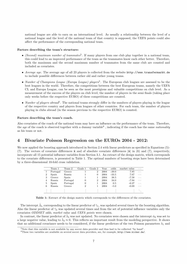
We now applied the boosting approach introduced in Section 2.4 with linear predictors as specified in Equations (5)-(7). The vectors of covariate differences x and of absolute covariate differences |x| in (6) and (7), respectively,incorporate all 15 potential influence variables from Section 3.1. An extract of the design matrix, which correspondsto the covariate differences, is presented in Table 1. The optimal numbers of boosting steps have been determinedby a three-dimensional 10-fold cross validation.

Team 1 Team 2 Goals 1 Goals 2 Year odds market value · · ·1 Portugal Greece 1 2 2004 -39.0 7.85 · · ·2 Spain Russia 1 0 2004 -33.5 7.67 · · ·3 Greece Spain 1 1 2004 38.5 -7.58 · · ·4 Russia Portugal 0 2 2004 34.0 -7.94 · · ·5 Spain Portugal 0 1 2004 0.5 -0.27 · · ·6 Russia Greece 2 1 2004 -5.0 -0.09 · · ·...

......

......

......

.... . .

Table 1: Extract of the design matrix which corresponds to the differences of the covariates.

The intercept β0, corresponding to the linear predictor of γ1, was updated several times by the boosting algorithm.Also the linear predictor of γ2 was updated several times and from the set of potential influence variables only thecovariates ODDSET odds, market value and UEFA points were chosen.

In contrast, the linear predictor of λ3 was not updated. No covariates were chosen and the intercept α0 was set toa large negative value, leading to λ3 ≈ 0. This reflects an important result from the modeling perspective. It showsthat no additional covariance needs to be considered, if the linear predictors of the two Poisson parameters λ1 and

5Note that this variable is not available by any soccer data provider and thus had to be collected “by hand”.6These two variables are available on several soccer data providers, see, for example, http://www.kicker.de/.

7

λ2, in our re-parametrization reflected by γ2, already contain informative covariate information from both teamsand, hence, already induce a certain amount of (negative) correlation. Instead, on the EURO 2004-2012 data twoindependent Poisson distributions can be used for the two numbers of goals of the matches, if the linear predictorof both Poisson parameters each contains covariate information (here in the form of differences) of both competingteams.

Altogether, we obtained a quite simple model with the following estimates (corresponding to scaled covariateinformation):

• γ1 = exp(β0) with β0 = 0.176

=⇒ γ1 = exp(β0) = 1.192; the parameter reflects the average number of goals, if two teams with equalcovariates play against each other

• γ2 = exp((x1 − x2)Tβββ) = exp(xTβββ) with (βodds, βmarketvalue, βUEFApoints) = (−0.120, 0.143, 0.029)

• λ3 = exp(α0 + |x1 − x2|Tααα) = exp(α0 + |x|Tααα) with α0 = −9.21, ααα = 0

=⇒ λ3 ≈ 0; no (additional) covariance between scores of both teams

Hence, our final model for match scores is based on these estimates and, regarding the findings with respect to λ3,on two independent Poisson distributions with parameters λ1 = γ1γ2 and λ2 = γ1/γ2. Based on this final model,in the following different simulation studies were applied.

4.1 Probabilities for the UEFA European Championship 2016 Winner

For each match of the EURO 2016, the final model from the previous section is used to calculate the two distributionsof the scores of the two competing teams. For this purpose, for the two competing teams in a match the covariatedifferences of the three selected covariates ODDSET odds, market value and UEFA points have to be calculated inorder to be able to compute an estimate of the linear predictor of the parameter γ2. Then, the match result canbe drawn randomly from these predicted distributions, i.e. G1 ∼ Poisson(λ1), G2 ∼ Poisson(λ2), with estimates

λ1 = γ1γ2 and λ2 = γ1/γ2. Note here that being able to draw exact match outcomes for each match constitutes anadvantage in comparison to several alternative prediction approaches, as this allows to precisely follow the officialUEFA rules when determining the final group standings7. If a match in the knockout stage ended in a draw, wesimulated another 30 minutes of extra time using scoring rates equal to 1/3 of the 90 minutes rates, i.e. using

Poisson parameters λ1/3 and λ2/3. If the match then still ended in a draw, the winner was calculated simply bycoin flip, reflecting a penalty shoot out.

The whole tournament was simulated 1,000,000 times. Based on these simulations, for each of the 24 participatingteams probabilities to reach the next stage and, finally, to win the tournament are obtained. These are summarizedin Table 2 together with the winning probabilities based on the ODDSET odds for comparison. In contrast to mostother prediction approaches for the current UEFA European championship favoring France (see, for example, Zeileiset al., 2016; Goldman-Sachs Economics Research, 2016), we get a neck-and-neck race between Spain and Germany,finally with better chances for Spain. The major reason for this is that in the simulations with a high probabilityboth Spain and Germany finish their groups on the first place and then face each other in the final. In a direct duel,the model concedes Spain a thin advantage with a winning probability of 51.1% against 48.9%. The favorites Spainand Germany are followed by the teams of France, England, Belgium and Portugal. This also shows how unlikely

7The final group standings are determined by the number of points. If two or more teams are equal on points after completion ofthe group matches, specific tie-breaking criteria are applied: if two or more teams are equal on points, the first tie-breaking criteria arematches between teams in question (1. obtained points; 2. goal difference; 3. higher number of goals scored). 4. if teams still havean equal ranking, criteria 1 to 3 are applied once again, exclusively to the matches between the teams in question to determine theirfinal rankings. If teams still have an equal ranking, all matches in the group are considered (5. goal difference; 6. higher number ofgoals scored). 7. if only two teams have the same number of points, and they were tied according to criteria 1-6 after having met inthe last round of the group stage, their ranking is determined by a direct penalty shoot-out (this criterion would not be used if three ormore teams had the same number of points.). 7. fair play conduct (yellow card: 1 point, red card: 3 points); 8. Position in the UEFAnational team coefficient ranking system.

Note that due to the augmentation from 16 to 24 teams, also the four best third-placed teams qualified for the newly introducedround-of-sixteen. For the determination of the four best third-placed teams also specific criteria are used: 1. obtained points; 2. goaldifference; 3. higher number of goals scored; 4. fair play conduct; 5. Position in the UEFA national team coefficient ranking system.Note that depending on which third-placed teams qualify from groups, several different options for the round-of-sixteen have to be takeninto account.

8

in advance of the tournament the triumph of the Portuguese team was assessed. While according to the bookmakerODDSET only a probability of 4.5% was expected, after all our model assigned an increased probability of 5.5% tothis event.

Round of 16 Quarter Finals Semi Finals Final European Champion Oddset

Spain 95.4 72.9 52.3 35.1 21.8 13.9Germany 99.3 79.5 51.3 34.4 21.0 16.9

France 97.5 71.9 48.2 25.8 13.8 18.9England 95.2 69.4 43.4 23.9 12.9 9.2Belgium 93.9 58.7 32.8 18.7 9.5 7.3Portugal 92.5 52.3 27.4 12.6 5.5 4.5

Italy 87.7 47.6 23.8 11.4 4.8 5.3Croatia 73.2 35.3 16.8 7.3 2.7 3.2Poland 86.0 42.2 15.6 5.5 1.6 2Austria 79.1 34.0 13.4 4.4 1.3 2.7

Switzerland 77.9 35.8 13.3 4.3 1.2 1.6Turkey 56.1 21.2 8.3 2.8 0.8 1.6Wales 65.6 27.4 9.6 2.8 0.8 1.6

Russia 62.3 25.1 8.6 2.5 0.6 1.3Ukraine 71.0 25.8 7.7 2.0 0.4 1Iceland 61.7 20.0 6.2 1.5 0.3 1.6

Czech Rep. 42.5 13.6 4.6 1.3 0.3 1.6Slovakia 44.5 13.6 3.6 0.8 0.2 1Sweden 42.9 11.2 3.3 0.8 0.1 1Ireland 41.7 10.6 3.1 0.7 0.1 1

Romania 45.6 12.3 2.8 0.5 0.1 0.8Albania 41.3 10.4 2.2 0.4 0.1 0.8

Hungary 37.1 8.1 1.8 0.3 0.0 0.8Nor. Ireland 10.0 1.0 0.1 0.0 0.0 0.4

Table 2: Estimated probabilities (in %) for reaching the different stages in the UEFA European championship 2016 for all24 teams based on 1,000,000 simulation runs of the UEFA European championship 2016 together with winning probabilitiesbased on the ODDSET odds.

4.2 Most probable tournament outcome

Finally, based on the 1,000,000 simulations, we also provide the most probable tournament outcome. Here, for eachof the six groups we selected the most probable final group standing regarding the complete order of the places oneto four. The results together with the corresponding probabilities are presented in Table 3.

A B C D E F

1 France England Germany Spain Belgium Portugal2 Switzerland Wales Poland Croatia Italy Austria3 Romania Russia Ukraine Turkey Sweden Iceland4 Albania Slovakia Nor. Ireland Czech Rep. Ireland Hungary

21.2% 15.1% 37.6% 17.7% 17.5% 16.9%

Table 3: Most probable final group standings together with the corresponding probabilities for the UEFA European cham-pionship 2016 based on 1,000,000 simulation runs

It is obvious that there are large differences with respect to the groups’ balances. While in Group A the modelforecasts the most likely final group standing of the four teams with a somewhat higher probabilities of 37.6%, theother groups seem to be closer.

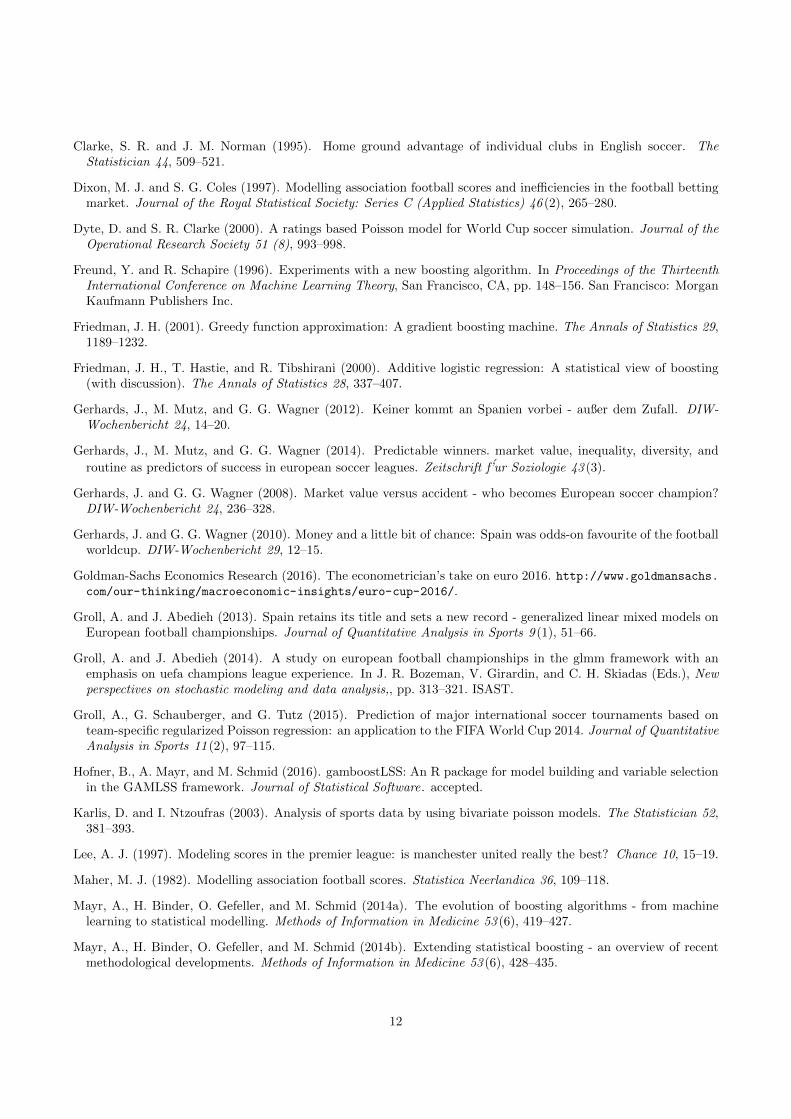
Based on the most probable group standings, we also provide the most probable course of the knockout stage,compare Figure 1. However, note that the most probable round-of-sixteen cannot directly be concluded from the

9

most probable final group standings shown in Table 3, as it is depending on which teams turn out to be the four bestthird-placed teams. For this reason, the knockout stage in Figure 1 starts with the most frequent constellation of theround-of-sixteen, which in fact still is extremely unlikely, as it occurred only 25 times out of the 1,000,000 simulationruns. Below each tournament stage the probability for the displayed combination of matches is displayed. Finally,according to the most probable tournament course the Spanish team would have won the European championship2016. After all, obviously even this ’most probable’ outcome is still extremely unlikely to happen because of themyriad of possible constellations. Hence, deviations of the true tournament outcome from the model’s most probableone are not only possible, but very likely.

ESPGER - ESP

ESP - ENG

POL - ESP

SUI - POL52%

ESP - ICE 85%

79%

ENG - POR

ENG - CRO65%

POR - ITA 51%

60% 58%

ESP - FRA

GER - BEL

GER - WAL81%

BEL - TUR 72%

59%

FRA - AUT

FRA - UKR81%

RUS - AUT 55%

73%

57%

51%

0.0025% 0.14% 2.65% 8.87% 21.8%

Figure 1: Most probable course of the knockout stage together with corresponding probabilities for the UEFA Europeanchampionship 2016 based on 1,000,000 simulation runs.

4.3 Prediction power

In the following, we try to asses the performance of our model with respect to prediction. We collected the “three-way” odds8 for all 51 matches of the EURO 2016 from the online bookmaker Tipico (https://www.tipico.de/de/online-sportwetten/). By taking the three quantities pr = 1/oddsr, r ∈ {1, 2, 3} and by normalizing with

c :=∑3r=1 pr in order to adjust for the bookmaker’s margins, the odds can be directly transformed into probabilities

using pr = pr/c9. On the other hand, let G1 and G2 denote the random variables representing the number of goals

scored by two competing teams in a match. Then, we can compute the same probabilities by approximatingp1 = P (G1 > G2), p2 = P (G1 = G2) and p3 = P (G1 < G2) for each of the 51 matches of the EURO 2016 using

the corresponding Poisson distributions G1 ∼ Poisson(λ1), G2 ∼ Poisson(λ2), where the estimates λ1 and λ2are obtained by our regression model. Based on these predicted probabilities, the average probability of a correctprediction of a EURO 2016 match can be obtained. For the true match outcomes ωm ∈ {1, 2, 3},m = 1, . . . , 51, it

is given by pthree-way := 151

∑51m=1 p

δ1ωm1m p

δ2ωm2m p

δ3ωm3m , with δrm denoting Kronecker’s delta. The quantity pthree-way

serves as a useful performance measure for a comparison of the predictive power of the model and the bookmaker’sodds and is shown for both data sets in Table 4. It is striking that the predictive power of our model outperformsthe bookmaker’s odds, especially if one has in mind that the bookmaker’s odds are usually released just some days

8Three-way odds consider only the tendency of a match with the possible results victory of team 1, draw or defeat of team 1 andare usually fixed some days before the corresponding match takes place.

9The transformed probabilities only serve as an approximation, based on the assumption that the bookmaker’s margins follow adiscrete uniform distribution on the three possible match tendencies.

10

before the corresponding match takes place and, hence, are able to include the latest performance trends of bothcompeting teams. This reflects a quite favorable result.

If one puts one’s trust into the model and its predicted probabilities, the following betting strategy can be applied:for every match one would bet on the three-way match outcome with the highest expected return, which can becalculated as the product of the model’s predicted probability and the corresponding three-way odd offered by thebookmakers. We applied this strategy to our model’s results, yielding a return of 30.28%, when for all 51 matchesequal-sized bets are placed. This is also a very satisfying result.

boosted bivariate Poisson model Tipico odds

42.22% 39.23%

Table 4: Average probability pthree-way of a correct prediction of a UEFA European championship 2016 match for our modeland the Tipico odds.

5 Concluding remarks

A bivariate Poisson model for the number of goals scored by soccer teams facing each other in international tourna-ment matches is set up. As an application, the UEFA European championships 2004-2012 serve as the data basisfor an analysis of the influence of several covariates on the success of national teams in terms of the number ofgoals they score in single matches. Procedures for variable selection based on boosting methods, implemented inthe R-package gamboostLSS, are used.

The boosting method selected only three covariates for the two Poisson parameters λ1 and λ2, namely theODDSET odds, the market value and the UEFA points, while for the covariance parameter λ3 no covariates wereselected and the parameter was in fact estimated to be zero. This reflects an important general result for themodeling of soccer data. It shows that on the EURO 2004-2012 data no additional (positive) covariance needs to beconsidered. Hence, instead of the bivariate Poisson distribution two independent Poisson distributions can be used,if the two corresponding Poisson parameters λ1 and λ2 already contain covariate information from both teams, and,in this way already induce a certain amount of (negative) correlation.

The obtained sparse model was then used for simulation of the UEFA European championship 2016. Accordingto these simulations, Spain, Germany and France turned out to be the top favorites for winning the title, with anadvantage for Spain. Besides, the most probable tournament outcome is provided. An analysis of the predictivepower of the model yielded very satisfactory results.

A major part of the statistical novelty of the presented work lies in the combination of boosting methods witha bivariate Poisson model. While the bivariate Poisson model enables explicit modeling of the covariance struc-ture between match scores, the boosting method allows to include many covariates simultaneously and performsautomatic variable selection.

Acknowledgement

We are grateful to Falk Barth and Johann Summerer from the ODDSET-Team for providing us all necessary oddsdata and to Sven Grothues from the Transfermarkt.de-Team for the pleasant collaboration.

References

Bernard, A. B. and M. R. Busse (2004). Who wins the olympic games: Economic developement and medall totals.The Review of Economics and Statistics 86 (1), 413–417.

Brown, T. D., J. L. V. Raalte, B. W. Brewer, C. R. Winter, A. E. Cornelius, and M. B. Andersen (2002). Worldcup soccer home advantage. Journal of Sport Behavior 25, 134–144.

Carlin, J. B., L. C. Gurrin, J. A. C. Sterne, R. Morley, and T. Dwyer (2005). Regression models for twin studies:a critical review. International Journal of Epidemiology B57, 1089–1099.

11

Clarke, S. R. and J. M. Norman (1995). Home ground advantage of individual clubs in English soccer. TheStatistician 44, 509–521.

Dixon, M. J. and S. G. Coles (1997). Modelling association football scores and inefficiencies in the football bettingmarket. Journal of the Royal Statistical Society: Series C (Applied Statistics) 46 (2), 265–280.

Dyte, D. and S. R. Clarke (2000). A ratings based Poisson model for World Cup soccer simulation. Journal of theOperational Research Society 51 (8), 993–998.

Freund, Y. and R. Schapire (1996). Experiments with a new boosting algorithm. In Proceedings of the ThirteenthInternational Conference on Machine Learning Theory, San Francisco, CA, pp. 148–156. San Francisco: MorganKaufmann Publishers Inc.

Friedman, J. H. (2001). Greedy function approximation: A gradient boosting machine. The Annals of Statistics 29,1189–1232.

Friedman, J. H., T. Hastie, and R. Tibshirani (2000). Additive logistic regression: A statistical view of boosting(with discussion). The Annals of Statistics 28, 337–407.

Gerhards, J., M. Mutz, and G. G. Wagner (2012). Keiner kommt an Spanien vorbei - außer dem Zufall. DIW-Wochenbericht 24, 14–20.

Gerhards, J., M. Mutz, and G. G. Wagner (2014). Predictable winners. market value, inequality, diversity, and

routine as predictors of success in european soccer leagues. Zeitschrift f’ur Soziologie 43 (3).

Gerhards, J. and G. G. Wagner (2008). Market value versus accident - who becomes European soccer champion?DIW-Wochenbericht 24, 236–328.

Gerhards, J. and G. G. Wagner (2010). Money and a little bit of chance: Spain was odds-on favourite of the footballworldcup. DIW-Wochenbericht 29, 12–15.

Goldman-Sachs Economics Research (2016). The econometrician’s take on euro 2016. http://www.goldmansachs.com/our-thinking/macroeconomic-insights/euro-cup-2016/.

Groll, A. and J. Abedieh (2013). Spain retains its title and sets a new record - generalized linear mixed models onEuropean football championships. Journal of Quantitative Analysis in Sports 9 (1), 51–66.

Groll, A. and J. Abedieh (2014). A study on european football championships in the glmm framework with anemphasis on uefa champions league experience. In J. R. Bozeman, V. Girardin, and C. H. Skiadas (Eds.), Newperspectives on stochastic modeling and data analysis,, pp. 313–321. ISAST.

Groll, A., G. Schauberger, and G. Tutz (2015). Prediction of major international soccer tournaments based onteam-specific regularized Poisson regression: an application to the FIFA World Cup 2014. Journal of QuantitativeAnalysis in Sports 11 (2), 97–115.

Hofner, B., A. Mayr, and M. Schmid (2016). gamboostLSS: An R package for model building and variable selectionin the GAMLSS framework. Journal of Statistical Software. accepted.

Karlis, D. and I. Ntzoufras (2003). Analysis of sports data by using bivariate poisson models. The Statistician 52,381–393.

Lee, A. J. (1997). Modeling scores in the premier league: is manchester united really the best? Chance 10, 15–19.

Maher, M. J. (1982). Modelling association football scores. Statistica Neerlandica 36, 109–118.

Mayr, A., H. Binder, O. Gefeller, and M. Schmid (2014a). The evolution of boosting algorithms - from machinelearning to statistical modelling. Methods of Information in Medicine 53 (6), 419–427.

Mayr, A., H. Binder, O. Gefeller, and M. Schmid (2014b). Extending statistical boosting - an overview of recentmethodological developments. Methods of Information in Medicine 53 (6), 428–435.

12

Mayr, A., N. Fenske, B. Hofner, T. Kneib, and M. Schmid (2012). Generalized additive models for location, scaleand shape for high-dimensional data – a flexible aproach based on boosting. Journal of the Royal StatisticalSociety: Series C (Applied Statistics) 61 (3), 403–427.

McHale, I. G. and P. A. Scarf (2006). Forecasting international soccer match re- sults using bivariate discretedistributions. Technical Report 322, Working paper, Salford Business School.

McHale, I. G. and P. A. Scarf (2011). Modelling the dependence of goals scored by opposing teams in internationalsoccer matches. Statistical Modelling 41 (3), 219–236.

Pollard, R. (2008). Home advantage in football: A current review of an unsolved puzzle. The Open Sports SciencesJournal 1, 12–14.

Pollard, R. and G. Pollard (2005). Home advantage in soccer: A review of its existence and causes. InternationalJournal of Soccer and Science Journal 3 (1), 25–33.

Rue, H. and O. Salvesen (2000). Prediction and retrospective analysis of soccer matches in a league. Journal of theRoyal Statistical Society: Series D (The Statistician) 49 (3), 399–418.

Schmid, M. and T. Hothorn (2008). Boosting additive models using component-wise P-splines. ComputationalStatistics & Data Analysis 53, 298–311.

Schmid, M., S. Potapov, A. Pfahlberg, and T. Hothorn (2010). Estimation and regularization techniques forregression models with multidimensional prediction functions. Statistics and Computing 20, 139–150.

Zeileis, A., C. Leitner, and K. Hornik (2016). Predictive Bookmaker Consensus Model for the UEFA Euro 2016.Working Papers 2016-15, Faculty of Economics and Statistics, University of Innsbruck.

Appendix

A Correlation structure of the EURO 2004 - 2012 data

home GDP max1 max2 odds popu- ave. market FIFA UEFA CL UEFA age nationlation age value rank points players players coach coach

GDP -0.01max1 0.07 -0.31max2 0.03 -0.35 0.64odds 0.06 -0.12 -0.03 -0.19

population -0.14 -0.07 0.41 0.53 -0.52ave age -0.20 0.11 -0.09 -0.18 0.26 -0.36

market value -0.08 0.14 0.27 0.41 -0.75 0.49 -0.27FIFA rank 0.58 -0.09 0.03 -0.11 0.70 -0.27 -0.06 -0.52

UEFA points 0.06 -0.11 -0.33 -0.37 0.72 -0.54 0.12 -0.76 0.44CL players 0.07 0.01 0.29 0.33 -0.46 0.24 -0.42 0.82 -0.31 -0.48

UEFA players -0.17 -0.08 0.09 0.23 -0.28 0.46 -0.15 0.27 -0.24 -0.20 0.15age coach 0.08 0.00 0.00 0.08 0.15 -0.01 -0.06 -0.02 0.13 0.07 0.09 -0.19

nation coach 0.03 0.23 -0.03 -0.16 -0.17 0.12 -0.15 0.19 0.01 -0.16 0.11 0.10 -0.32legionnaires -0.04 0.15 -0.59 -0.72 0.26 -0.77 0.36 -0.45 0.01 0.55 -0.23 -0.35 0.00 0.01

Table 5: Correlation matrix of the considered variable differences for the EURO 2004 - 2012.

13