Wheat Crop Yield Prediction Using Deep LSTMModel

Sagarika Sharma∗†, Sujit Rai∗ ‡, Narayanan C. Krishnan §Indian Institute of Technology Ropar, India

†2017csb1012@iitrpr.ac.in, ‡2017csm1006@iitrpr.ac.in, §ckn@iitrpr.ac.in

Abstract—An in-season early crop yield forecast before harvestcan benefit the farmers to improve the production and enablevarious agencies to devise plans accordingly. We introduce areliable and inexpensive method to predict crop yields frompublicly available satellite imagery. The proposed method worksdirectly on raw satellite imagery without the need to extractany hand-crafted features or perform dimensionality reductionon the images. The approach implicitly models the relevance ofthe different steps in the growing season, and the various bandsin the satellite imagery. We evaluate the proposed approach ontehsil (block) level wheat predictions across several states in Indiaand demonstrate that it outperforms over existing methods byover 50%. We also show that incorporating additional contextualinformation such as the location of farmlands, water bodies, andurban areas helps in improving the yield estimates.

I. INTRODUCTION

India is predominantly an agrarian economy, with nearly70% of its rural households depending primarily on agriculturefor their livelihood. Approximately 82% of farmers are smalland marginal landowners (FAO, India at a glance [3]), which isestimated to grow to 91% by 2030. The marginal landholdingscombined with traditional modes of farming, and external fac-tors such as irregular rainfall, depletion of groundwater, etc.,result in the yield of crops in India still being below the worldaverage (Economic Survey 2015-16 [2]). Existing approachesfor estimating yield rely on manual surveys during the growingseason. The enormous costs and the manual effort requiredto conduct such studies makes it a cumbersome method topredict crop yields. At the same time, lack of reliable and upto date information on crop yield affects supply-demand stocksand export options. Thus, an in-season crop yield forecastcan benefit the farmers to improve production and enable thegovernment agencies to devise appropriate plans.

Remote sensing data is becoming an increasingly popularsource of data for developing models for various applicationssuch as poverty estimation [20], income prediction [16], yieldestimation [21], etc. The easy and inexpensive access, high-resolution imagery combined with increasing sophisticatedmodeling techniques, makes it a viable solution for many ofthese problems. In particular, multi-spectral satellite imageryhave information across a wide spectrum of wavelengths thatabundantly encode information related to land use such asvegetation, water bodies, urban areas, etc.

In this paper, we propose an approach for crop yield estima-tion from satellite imagery using deep learning techniques that

∗Authors with equal contribution.

have found success in traditional computer vision tasks. Unlikeprior methods that involve extracting hand-crafted features orrudimentary features such as histograms, our approach directlyworks on the satellite images. It allows the model to learnthe representations that are useful for the yield predictiontask. Often yield estimates in a geographical area dependon other factors such as nearby water bodies, urbanization,etc. While prior approaches to yield prediction do not takeinto account these factors, we incorporate these aspects byexplicitly weaving into our model the land use classificationdata. We model the temporal features in the data through adeep LSTM model. This allows our model to automaticallyidentify the relevance of the different growing steps and thesatellite image bands towards the yield prediction task.

We evaluate and validate our approach on the task of tehsil(block) level wheat prediction for seven states in India. Weuse the MODIS surface reflectance multi-spectral satelliteimages, along with the land use classification maps, to trainthe proposed deep learning models. The experimental resultsshow that our model can outperform traditional remote-sensingbased methods by 70% and recently introduced deep learningmodels by 54%. To the best of our knowledge, this is the firstmethod that yields promising results for crop yield predictionin the Indian context.

II. RELATED WORK

In recent years, remote sensing data has been widely usedin various sustainability applications such as land use classi-fication [5], infrastructure quality prediction [15], povertyestimation [20], population estimation [19] and income levelpredictions [16].

Crop yield estimation using remote sensing data has alsobeen explored over the past few years. Prasad et al. [17]employ a piece-wise linear regression and a non-linear Quasi-Newton multi-variate regression model to predict soybeanyield in the state of Iowa using normalized difference veg-etation index (NDVI), soil moisture, surface temperature, andrainfall data. Kuwata and Shibasaki [11] estimate county-level crop yield for the state of Illinois using MOD09A1derived EVI (Enhanced Vegetation Index), climate and otherenvironmental data by employing deep neural network andSVM. Johnson et al. [10] learn models to predict corn andsoybean yields from NDVI and daytime land surface tem-perature data (derived from the Aqua MODIS sensor productMYD11A2) using a regression tree. Mallick et al. [13] use

arX

iv:2

011.

0149

8v1

[cs

.CV

] 3

Nov

202

0

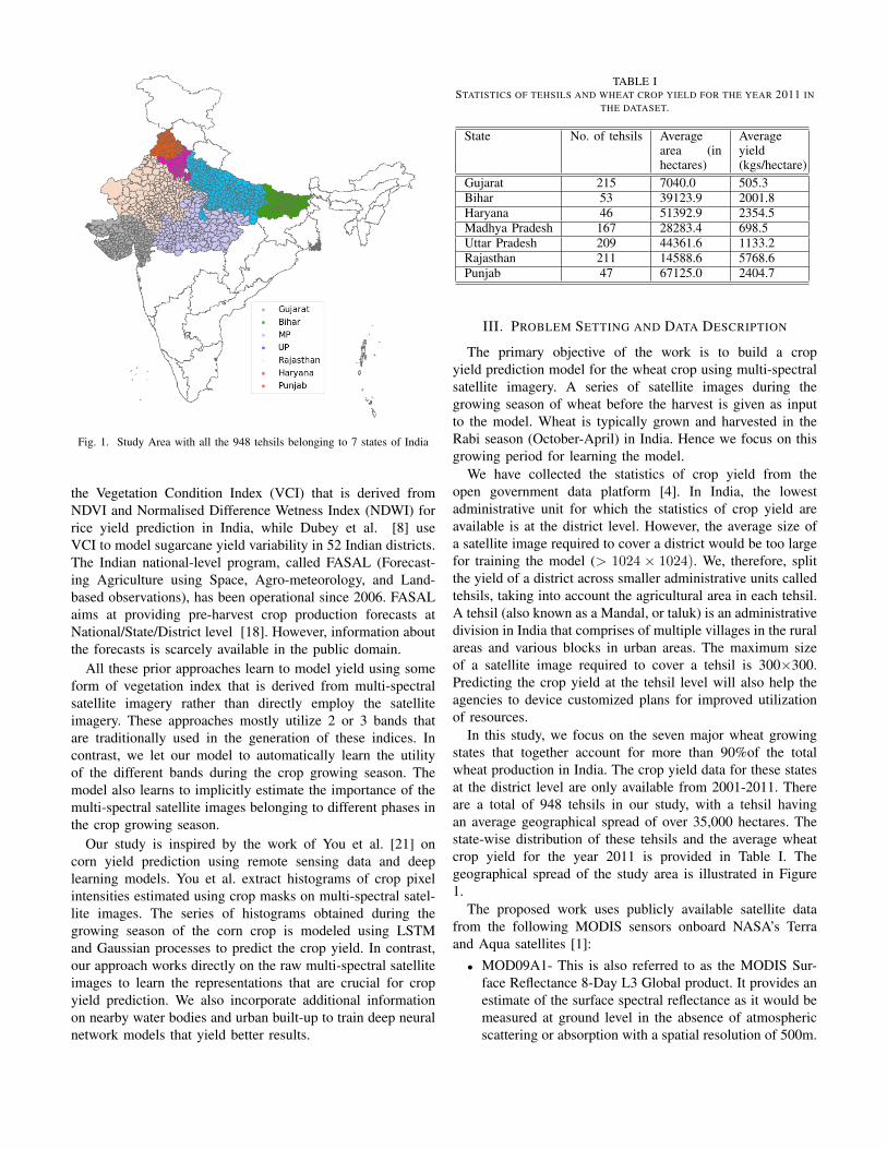
Fig. 1. Study Area with all the 948 tehsils belonging to 7 states of India

the Vegetation Condition Index (VCI) that is derived fromNDVI and Normalised Difference Wetness Index (NDWI) forrice yield prediction in India, while Dubey et al. [8] useVCI to model sugarcane yield variability in 52 Indian districts.The Indian national-level program, called FASAL (Forecast-ing Agriculture using Space, Agro-meteorology, and Land-based observations), has been operational since 2006. FASALaims at providing pre-harvest crop production forecasts atNational/State/District level [18]. However, information aboutthe forecasts is scarcely available in the public domain.

All these prior approaches learn to model yield using someform of vegetation index that is derived from multi-spectralsatellite imagery rather than directly employ the satelliteimagery. These approaches mostly utilize 2 or 3 bands thatare traditionally used in the generation of these indices. Incontrast, we let our model to automatically learn the utilityof the different bands during the crop growing season. Themodel also learns to implicitly estimate the importance of themulti-spectral satellite images belonging to different phases inthe crop growing season.

Our study is inspired by the work of You et al. [21] oncorn yield prediction using remote sensing data and deeplearning models. You et al. extract histograms of crop pixelintensities estimated using crop masks on multi-spectral satel-lite images. The series of histograms obtained during thegrowing season of the corn crop is modeled using LSTMand Gaussian processes to predict the crop yield. In contrast,our approach works directly on the raw multi-spectral satelliteimages to learn the representations that are crucial for cropyield prediction. We also incorporate additional informationon nearby water bodies and urban built-up to train deep neuralnetwork models that yield better results.

TABLE ISTATISTICS OF TEHSILS AND WHEAT CROP YIELD FOR THE YEAR 2011 IN

THE DATASET.

State No. of tehsils Averagearea (inhectares)

Averageyield(kgs/hectare)

Gujarat 215 7040.0 505.3Bihar 53 39123.9 2001.8Haryana 46 51392.9 2354.5Madhya Pradesh 167 28283.4 698.5Uttar Pradesh 209 44361.6 1133.2Rajasthan 211 14588.6 5768.6Punjab 47 67125.0 2404.7

III. PROBLEM SETTING AND DATA DESCRIPTION

The primary objective of the work is to build a cropyield prediction model for the wheat crop using multi-spectralsatellite imagery. A series of satellite images during thegrowing season of wheat before the harvest is given as inputto the model. Wheat is typically grown and harvested in theRabi season (October-April) in India. Hence we focus on thisgrowing period for learning the model.

We have collected the statistics of crop yield from theopen government data platform [4]. In India, the lowestadministrative unit for which the statistics of crop yield areavailable is at the district level. However, the average size ofa satellite image required to cover a district would be too largefor training the model (> 1024 × 1024). We, therefore, splitthe yield of a district across smaller administrative units calledtehsils, taking into account the agricultural area in each tehsil.A tehsil (also known as a Mandal, or taluk) is an administrativedivision in India that comprises of multiple villages in the ruralareas and various blocks in urban areas. The maximum sizeof a satellite image required to cover a tehsil is 300×300.Predicting the crop yield at the tehsil level will also help theagencies to device customized plans for improved utilizationof resources.

In this study, we focus on the seven major wheat growingstates that together account for more than 90%of the totalwheat production in India. The crop yield data for these statesat the district level are only available from 2001-2011. Thereare a total of 948 tehsils in our study, with a tehsil havingan average geographical spread of over 35,000 hectares. Thestate-wise distribution of these tehsils and the average wheatcrop yield for the year 2011 is provided in Table I. Thegeographical spread of the study area is illustrated in Figure1.

The proposed work uses publicly available satellite datafrom the following MODIS sensors onboard NASA’s Terraand Aqua satellites [1]:

• MOD09A1- This is also referred to as the MODIS Sur-face Reflectance 8-Day L3 Global product. It provides anestimate of the surface spectral reflectance as it would bemeasured at ground level in the absence of atmosphericscattering or absorption with a spatial resolution of 500m.

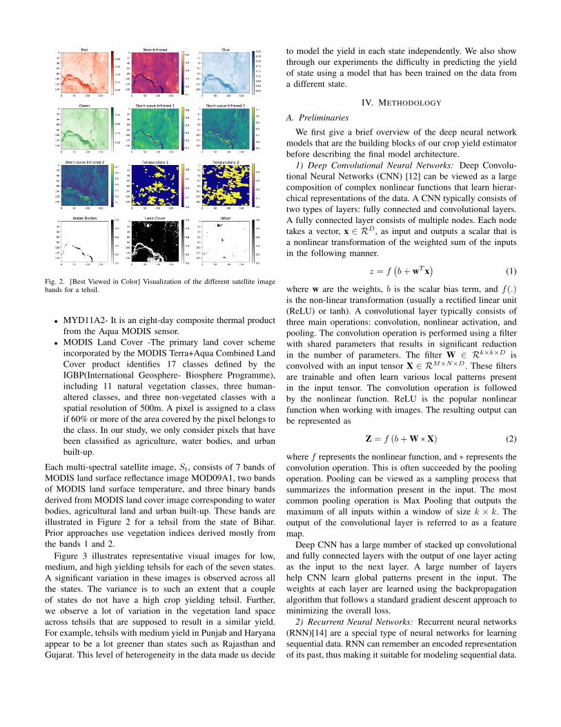
Fig. 2. [Best Viewed in Color] Visualization of the different satellite imagebands for a tehsil.

• MYD11A2- It is an eight-day composite thermal productfrom the Aqua MODIS sensor.

• MODIS Land Cover -The primary land cover schemeincorporated by the MODIS Terra+Aqua Combined LandCover product identifies 17 classes defined by theIGBP(International Geosphere- Biosphere Programme),including 11 natural vegetation classes, three human-altered classes, and three non-vegetated classes with aspatial resolution of 500m. A pixel is assigned to a classif 60% or more of the area covered by the pixel belongs tothe class. In our study, we only consider pixels that havebeen classified as agriculture, water bodies, and urbanbuilt-up.

Each multi-spectral satellite image, St, consists of 7 bands ofMODIS land surface reflectance image MOD09A1, two bandsof MODIS land surface temperature, and three binary bandsderived from MODIS land cover image corresponding to waterbodies, agricultural land and urban built-up. These bands areillustrated in Figure 2 for a tehsil from the state of Bihar.Prior approaches use vegetation indices derived mostly fromthe bands 1 and 2.

Figure 3 illustrates representative visual images for low,medium, and high yielding tehsils for each of the seven states.A significant variation in these images is observed across allthe states. The variance is to such an extent that a coupleof states do not have a high crop yielding tehsil. Further,we observe a lot of variation in the vegetation land spaceacross tehsils that are supposed to result in a similar yield.For example, tehsils with medium yield in Punjab and Haryanaappear to be a lot greener than states such as Rajasthan andGujarat. This level of heterogeneity in the data made us decide

to model the yield in each state independently. We also showthrough our experiments the difficulty in predicting the yieldof state using a model that has been trained on the data froma different state.

IV. METHODOLOGY

A. Preliminaries

We first give a brief overview of the deep neural networkmodels that are the building blocks of our crop yield estimatorbefore describing the final model architecture.

1) Deep Convolutional Neural Networks: Deep Convolu-tional Neural Networks (CNN) [12] can be viewed as a largecomposition of complex nonlinear functions that learn hierar-chical representations of the data. A CNN typically consists oftwo types of layers: fully connected and convolutional layers.A fully connected layer consists of multiple nodes. Each nodetakes a vector, x ∈ RD, as input and outputs a scalar that isa nonlinear transformation of the weighted sum of the inputsin the following manner.

z = f(b+ wT x

)(1)

where w are the weights, b is the scalar bias term, and f(.)is the non-linear transformation (usually a rectified linear unit(ReLU) or tanh). A convolutional layer typically consists ofthree main operations: convolution, nonlinear activation, andpooling. The convolution operation is performed using a filterwith shared parameters that results in significant reductionin the number of parameters. The filter W ∈ Rk×k×D isconvolved with an input tensor X ∈ RM×N×D. These filtersare trainable and often learn various local patterns presentin the input tensor. The convolution operation is followedby the nonlinear function. ReLU is the popular nonlinearfunction when working with images. The resulting output canbe represented as

Z = f (b+ W ∗ X) (2)

where f represents the nonlinear function, and ∗ represents theconvolution operation. This is often succeeded by the poolingoperation. Pooling can be viewed as a sampling process thatsummarizes the information present in the input. The mostcommon pooling operation is Max Pooling that outputs themaximum of all inputs within a window of size k × k. Theoutput of the convolutional layer is referred to as a featuremap.

Deep CNN has a large number of stacked up convolutionaland fully connected layers with the output of one layer actingas the input to the next layer. A large number of layershelp CNN learn global patterns present in the input. Theweights at each layer are learned using the backpropagationalgorithm that follows a standard gradient descent approach tominimizing the overall loss.

2) Recurrent Neural Networks: Recurrent neural networks(RNN)[14] are a special type of neural networks for learningsequential data. RNN can remember an encoded representationof its past, thus making it suitable for modeling sequential data.

Fig. 3. [Best Viewed in Color] Visual images for different yield levels for the seven states

Fig. 4. The proposed CNN-LSTM architecture for predicting crop yield from a sequence of multi-spectral satellite imagery

Given a sequential data x1, x2, . . . , xT for T time steps, theoutput yt at time step t, is a function of the input at time stepxt and the hidden state zt−1 at time step t−1, can be definedas follows

zt = f(wTt xt + uT zt−1) (3)

yt = g(vT zt) (4)

where, w, u and v are the weights applied on xt, zt−1 andzt respectively and f and g are the non-linear activationfunctions. As, output is dependent on the hidden states ofthe previous time steps, the back propagation through timealgorithm for updating the weights can result in the problemof vanishing or exploding gradients [6].

LSTM [9], a special kind of RNN, were introduced toovercome this issue by integrating a gradient superhighwayin the form of a cell state c, in addition to the hidden stateh. The LSTM model has gates for providing the ability toadd and remove information to the cell state. The forget gatedecides the information to be deleted from the cell state andcan be defined as follows

ft = σ(wTf [ht−1, xt] + bf ) (5)

The input gate that determines the information that should beadded to the cell state is defined as

it = σ(wTi [ht−1, xt] + bi) (6)

The cell state ct is obtained by using both ft and it in thefollowing manner

ct = tanh(wTc [ht−1, xt] + bc) (7)

ct = fTt ct−1 + iTt ct (8)

Similarly, the hidden state ht and output state ot of the LSTMare defined as

ot = σ(wTo [ht−1, xt] + bo) (9)

ht = oTt tanh(ct) (10)

LSTM is more effective in modeling longer sequences thana simple RNN due to a more effective gradient flow duringbackpropagation.

B. Crop Yield Prediction Model Architecture

We directly input the multi-spectral satellite imagery toour deep neural network model. The motivation for using

the raw imagery is to be able to extract features relatingto the spatial location of crop pixels and the properties ofneighboring regions such as water bodies, urban landscapes,etc. We hypothesize that these parameters influence the cropyield.

The proposed deep network has three modules. The firstmodule is a CNN that learns to extract relevant features fromthe images. The second module is an LSTM that determinesthe temporal relationship during the crop growing season. Thethird module is a fully connected network that finally predictsthe crop yield.

The proposed CNN-LSTM architecture is illustrated in Fig-ure 4. The input to the network is a sequence S1, S2, ..., S24,where St is a multi-spectral image of size 300 × 300 × b attime t, where b refers to the number of bands. In the proposedmodel, we use 12 bands. The entire sequence is used duringtraining and validation. During testing, we vary the sequencelength between 1 and 23.

The image St at every time step t is first passed to theCNN feature extractor to extract the features fst present in theimage. The CNN feature extractor consists of 5 convolutionallayers, each having 16 filters of size [3×3] with a stride size of[2×2] and Leaky-ReLU as the activation function. The choiceof the number of convolutional layers and filters in each layerwas constrained by the computational resources. There is nopooling operation due to the use of strided convolutions. Theoutput of the convolutional feature extractor is flattened intoa 1024 dimensional vector. The features extracted for eachof the T time steps are stacked and passed on to the LSTMmodel.

The LSTM model is used to encode the temporal propertiesacross the growing season. The model consists of 3 LSTMlayers. Each LSTM layer contains 512 nodes that use Leaky-ReLU as the activation function. Dropout with a keep proba-bility of 75% is applied to the output of each LSTM layer. The512-dimensional feature vector obtained from the last LSTMlayer is passed to yield predictor.

The yield predictor consists of 3 fully connected layerswith the first two layers using Leaky-ReLU as the activationfunction. The yield predictor outputs yt the crop yield inkilograms per hectare for the input sequence until time step t.An L2-loss is applied to the predictions corresponding to eachtime step against the actual output yt. Note that the actual yieldat every time step is the same as the yield at the last time step.The overall loss of the entire CNN-LSTM network is definedas follows

Loss =

24∑t=1

(yt − yt)2 (11)

Applying the L2-loss at each time step increases the flowof gradients to the shared LSTM weights, thus increasingprediction accuracy and faster convergence. This also helpsus to predict the yield for intermediate stages of the growingseason. Given a test sequence of 24 images, the overall yield isobtained by averaging the yield predicted by the CNN-LSTMmodel at every time step. Figure 5 presents the decrease in the

Fig. 5. Progression of training and validation error as a function of epochs

training and validation loss as a function of epochs. We usethe model resulting in the lowest validation error for predictingthe yield on the test set.

V. EXPERIMENTS AND RESULTS

A. Comparison Against Baselines

We compare the performance of the proposed model againstapproaches in the literature that use handcrafted features fromthe satellite imagery like NDVI and VCI. We train DecisionTrees [10], Random Forests, and Ridge Regression models [7]using a feature vector of NDVI values derived from each ofthe 24 satellite images spanning the entire growing season.We also perform step-wise regression with VCI [13]. Wecompare our approach against the LSTM+Gaussian Processmodel [21] on the histogram of crop pixels. The parameters forall these approaches were fine-tuned using a cross-validationprocess. We denote our proposed model that uses raw satelliteimagery and contextual information such as water bodies, anagricultural area, and urban landscape as CNN-LSTM-12.

We use root mean square error (RMSE) in kgs/hectarefor comparing the performance of the different models. Thetraining set consists of data within the years 2001-2009, thevalidation set used for tuning the parameters was from theyear 2010, and the test set consisted of the data from the year2011. The results for the different states are presented in TableII. It can be observed that the proposed approach performssignificantly better than the methods that use NDVI and VCIfeatures by over 70%. Further, our approach performs betterthan the LSTM+GP approach of You et al. by over 54%. Weattribute this improvement in the performance of the CNN-LSTM-12 model to its ability to learn features relevant tothe task of crop yield prediction, instead of using handcraftedfeatures like a histogram.

The crop yield error plots at the tehsil level for everystate are presented in Figure 6. It can be observed that for amajority of the tehsils across all the states, the CNN-LSTM-12 model is under-predicting the yield marginally. This isfurther verified by the plot on the left-hand side in Figure7. This compares the error against the size of the tehsil. Weobserve that for large tehsils, the model always underestimatedthe yield. However, the number of such large area tehsils is

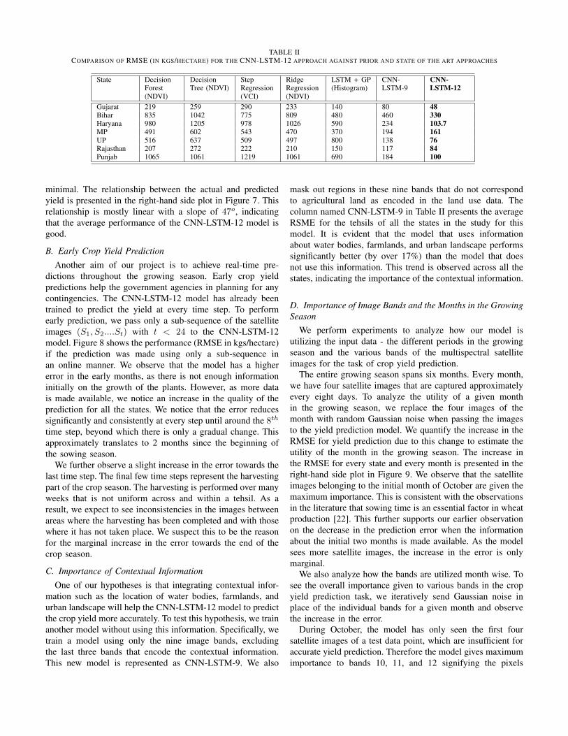
TABLE IICOMPARISON OF RMSE (IN KGS/HECTARE) FOR THE CNN-LSTM-12 APPROACH AGAINST PRIOR AND STATE OF THE ART APPROACHES

State DecisionForest(NDVI)

DecisionTree (NDVI)

StepRegression(VCI)

RidgeRegression(NDVI)

LSTM + GP(Histogram)

CNN-LSTM-9

CNN-LSTM-12

Gujarat 219 259 290 233 140 80 48Bihar 835 1042 775 809 480 460 330Haryana 980 1205 978 1026 590 234 103.7MP 491 602 543 470 370 194 161UP 516 637 509 497 800 138 76Rajasthan 207 272 222 210 150 117 84Punjab 1065 1061 1219 1061 690 184 100

minimal. The relationship between the actual and predictedyield is presented in the right-hand side plot in Figure 7. Thisrelationship is mostly linear with a slope of 47o, indicatingthat the average performance of the CNN-LSTM-12 model isgood.

B. Early Crop Yield Prediction

Another aim of our project is to achieve real-time pre-dictions throughout the growing season. Early crop yieldpredictions help the government agencies in planning for anycontingencies. The CNN-LSTM-12 model has already beentrained to predict the yield at every time step. To performearly prediction, we pass only a sub-sequence of the satelliteimages (S1, S2....St) with t < 24 to the CNN-LSTM-12model. Figure 8 shows the performance (RMSE in kgs/hectare)if the prediction was made using only a sub-sequence inan online manner. We observe that the model has a highererror in the early months, as there is not enough informationinitially on the growth of the plants. However, as more datais made available, we notice an increase in the quality of theprediction for all the states. We notice that the error reducessignificantly and consistently at every step until around the 8th

time step, beyond which there is only a gradual change. Thisapproximately translates to 2 months since the beginning ofthe sowing season.

We further observe a slight increase in the error towards thelast time step. The final few time steps represent the harvestingpart of the crop season. The harvesting is performed over manyweeks that is not uniform across and within a tehsil. As aresult, we expect to see inconsistencies in the images betweenareas where the harvesting has been completed and with thosewhere it has not taken place. We suspect this to be the reasonfor the marginal increase in the error towards the end of thecrop season.

C. Importance of Contextual Information

One of our hypotheses is that integrating contextual infor-mation such as the location of water bodies, farmlands, andurban landscape will help the CNN-LSTM-12 model to predictthe crop yield more accurately. To test this hypothesis, we trainanother model without using this information. Specifically, wetrain a model using only the nine image bands, excludingthe last three bands that encode the contextual information.This new model is represented as CNN-LSTM-9. We also

mask out regions in these nine bands that do not correspondto agricultural land as encoded in the land use data. Thecolumn named CNN-LSTM-9 in Table II presents the averageRSME for the tehsils of all the states in the study for thismodel. It is evident that the model that uses informationabout water bodies, farmlands, and urban landscape performssignificantly better (by over 17%) than the model that doesnot use this information. This trend is observed across all thestates, indicating the importance of the contextual information.

D. Importance of Image Bands and the Months in the GrowingSeason

We perform experiments to analyze how our model isutilizing the input data - the different periods in the growingseason and the various bands of the multispectral satelliteimages for the task of crop yield prediction.

The entire growing season spans six months. Every month,we have four satellite images that are captured approximatelyevery eight days. To analyze the utility of a given monthin the growing season, we replace the four images of themonth with random Gaussian noise when passing the imagesto the yield prediction model. We quantify the increase in theRMSE for yield prediction due to this change to estimate theutility of the month in the growing season. The increase inthe RMSE for every state and every month is presented in theright-hand side plot in Figure 9. We observe that the satelliteimages belonging to the initial month of October are given themaximum importance. This is consistent with the observationsin the literature that sowing time is an essential factor in wheatproduction [22]. This further supports our earlier observationon the decrease in the prediction error when the informationabout the initial two months is made available. As the modelsees more satellite images, the increase in the error is onlymarginal.

We also analyze how the bands are utilized month wise. Tosee the overall importance given to various bands in the cropyield prediction task, we iteratively send Gaussian noise inplace of the individual bands for a given month and observethe increase in the error.

During October, the model has only seen the first foursatellite images of a test data point, which are insufficient foraccurate yield prediction. Therefore the model gives maximumimportance to bands 10, 11, and 12 signifying the pixels

Fig. 6. Tehsil level error heat maps for all the 7 states.

Fig. 7. The left figure is the plot of the difference between predicted and actual yield against the area of the tehsils and the plot on the right side illustratesthe relationship between predicted and actual yield of all tehsils.

Fig. 8. Accuracy of early prediction

belonging to water bodies, agriculture, and urban built-up. Asthe model sees more satellite images, it has already recognizedthe type and the context of each pixel in the sequence ofsatellite images. Hence, it starts giving lesser importance tothe last three bands. The trend that is visible in all the statesis that when a band is given significance in a particularmonth, in the subsequent month, it is immediately given lessimportance, as the model now gives importance to other bands.The temperature band is consistently given high importance in

the later months.

E. Generalizability

We also try to see how similar different states are in terms ofheterogeneity of weather patterns, soil type, farming methods,etc. For this, we train our model on one state and test it onthe remaining states. The results are presented in Figure 10.We observe that the results when the test state is differentare quite poor, with a significant increase in the error (over1000 in some cases). This further supports our original ideaof modeling each state independently.

We had performed a couple of experiments before fixing thestate-wise models. A single model was trained using data from10 bands for all the states; however, the model was having highloss >520, while the average loss of state-wise models was<120 (<100 for some states). The LSTM+GP model on theentire dataset also gave similar losses.

VI. CONCLUSION

We introduce a reliable and inexpensive method to predictcrop yields from publicly available satellite imagery. Specif-ically, we learn a deep neural network model for predictingthe wheat crop yield for tehsils in India. The proposed methodworks directly on raw satellite imagery without the need toextract any hand-crafted features or perform dimensionalityreduction on the images. We have created a new datasetconsisting of a sequence of satellite images and the exact crop

Fig. 9. Increase in the RMSE when the images of a specific month are replaced with random noise.

Fig. 10. Error of models trained and tested on different states

yield for the years 2001-2011 covering a total of 948 tehsils.We use this dataset to train and evaluate the proposed approachon tehsil level wheat predictions. Our model outperformsover existing methods by over 50%. We also show thatincorporating additional contextual information such as thelocation of farmlands, water bodies, and urban areas helpsin improving the yield estimates.

VII. ACKNOWLEDGEMENT

We are grateful to Dr. Reet Kamal Tiwari and AksharTripathi for their inputs and assistance in understanding andcollecting the satellite data. We are also grateful to NVIDIACorporation for supporting this research through an academichardware grant.

REFERENCES

[1] Lp daac. https://lpdaac.usgs.gov/.[2] Union budget and economic survey. www.indiabudget.gov.in/

budget2016-2017/survey.asp.[3] “FAO.org.” India at a Glance — FAO in India — Food and Agriculture

Organization of the United Nations.[4] Open Government Data Platform India. https://aps.dac.gov.in/APY/

Public Report1.aspx, 2018.[5] A. Albert, J. Kaur, and M. C. Gonzalez. Using convolutional networks

and satellite imagery to identify patterns in urban environments at alarge scale. In Proceedings of the 23rd ACM SIGKDD InternationalConference on Knowledge Discovery and Data Mining, pages 1357–1366. ACM, 2017.

[6] Y. Bengio, P. Simard, P. Frasconi, et al. Learning long-term dependencieswith gradient descent is difficult. IEEE transactions on neural networks,5(2):157–166, 1994.

[7] D. K. Bolton and M. A. Friedl. Forecasting crop yield using remotelysensed vegetation indices and crop phenology metrics. Agricultural andForest Meteorology, 173:74–84, 2013.

[8] S. Dubey, A. Gavli, S. Yadav, S. Sehgal, and S. Ray. Remote sensing-based yield forecasting for sugarcane (saccharum officinarum l.) crop inindia. Journal of the Indian Society of Remote Sensing, 46(11):1823–1833, 2018.

[9] S. Hochreiter and J. Schmidhuber. Long short-term memory. Neuralcomputation, 9(8):1735–1780, 1997.

[10] D. M. Johnson. An assessment of pre-and within-season remotely sensedvariables for forecasting corn and soybean yields in the united states.Remote Sensing of Environment, 141:116–128, 2014.

[11] K. Kuwata and R. Shibasaki. Estimating crop yields with deep learningand remotely sensed data. In 2015 IEEE International Geoscience andRemote Sensing Symposium (IGARSS), pages 858–861. IEEE, 2015.

[12] Y. LeCun, L. Bottou, Y. Bengio, P. Haffner, et al. Gradient-basedlearning applied to document recognition. Proceedings of the IEEE,86(11):2278–2324, 1998.

[13] K. Mallick, J. Mukherjee, S. Bal, S. Bhalla, and S. Hundal. Real timerice yield forecasting over central punjab region using crop weatherregression model. Journal of Agrometeorology, 9(2):158–166, 2007.

[14] T. Mikolov, M. Karafiat, L. Burget, J. Cernocky, and S. Khudanpur.Recurrent neural network based language model. In Eleventh annualconference of the international speech communication association, 2010.

[15] B. Oshri, A. Hu, P. Adelson, X. Chen, P. Dupas, J. Weinstein, M. Burke,D. Lobell, and S. Ermon. Infrastructure quality assessment in africausing satellite imagery and deep learning. In Proceedings of the 24thACM SIGKDD International Conference on Knowledge Discovery &Data Mining, pages 616–625. ACM, 2018.

[16] S. M. Pandey, T. Agarwal, and N. C. Krishnan. Multi-task deep learningfor predicting poverty from satellite images. In Thirty-Second AAAIConference on Artificial Intelligence, 2018.

[17] A. K. Prasad, L. Chai, R. P. Singh, and M. Kafatos. Crop yield estimationmodel for iowa using remote sensing and surface parameters. Inter-national Journal of Applied Earth Observation and Geoinformation,8(1):26–33, 2006.

[18] S. S. Ray, S. Mamatha Neetu, and S. Gupta. Use of remote sensingin crop forecasting and assessment of impact of natural disasters:operational approaches in india. Crop monitoring for improved foodsecurity, 2014.

[19] C. Robinson, F. Hohman, and B. Dilkina. A deep learning approach forpopulation estimation from satellite imagery. In Proceedings of the 1stACM SIGSPATIAL Workshop on Geospatial Humanities, pages 47–54.ACM, 2017.

[20] M. Xie, N. Jean, M. Burke, D. Lobell, and S. Ermon. Transfer learningfrom deep features for remote sensing and poverty mapping. In ThirtiethAAAI Conference on Artificial Intelligence, 2016.

[21] J. You, X. Li, M. Low, D. Lobell, and S. Ermon. Deep gaussian processfor crop yield prediction based on remote sensing data. In Thirty-FirstAAAI Conference on Artificial Intelligence, 2017.

[22] M. Zubair and A. A. Khakwani. Effect of sowing dates on the yieldand yield components of different wheat varieties. Journal of Agronomy,5(1):106–110, 2006.