Welcome to Session 6. Today we will discuss the basic oligopoly models. Oligopoly is a prevalent form of market structure in which there are a handful of firms and each is large relative to the total industry. Examples include automobiles, airlines and computers.

•1

Oligopolies may arise due to scale/scope economies, patents and the need to spend money for brand recognition. Or capitalists may take strategic action to deter entry. Because there are only few firms in the industry, the strategy of each firm is affected by the other competitors. This makes management in oligopoly challenging as each firm must consider pricing, output, advertising decisions of all other firms in the market while making its own decisions. Also the firms in oligopoly will have to take into account that each firm in the market is also accounting for the decision of other competitors. To analyze equilibrium in the oligopoly market we assume that each firm is doing the best it can while taking into account its competitors decisions. The following models are used to study oligopoly in this session: Sweezy (Kinked-Demand) Model Cournot Model

•2

The Oligopoly environment includes the following features:

• Relatively few firms, usually less than 10.

Duopoly - two firms

Triopoly - three firms

• The products firms offer can be either differentiated or homogeneous.

• Firms’ decisions impact one another.

• Many different strategic variables are modeled:

No single oligopoly model.

To ease the complexity of analysis we will mostly use two firms. The results derived for two firms can then be extended to 3,4,5,6 etc. firms in an industry.

•3

Strategic interaction involves accounting for the fact that your actions affect the profits of your rivals and your rivals’ actions affect your profits. Or in other words each competitor takes the actions of its rival firms into account and assumes that the rival firms are doing exactly the same thing.

•4

The interdependence between firms holds for both homogenous and differentiated products. Consider a situation where several firms selling differentiated products compete in an oligopoly. A manager making a pricing decision in oligopoly needs to consider what happens to the price of other firms when the manager lowers or increases the price. The optimal decision of whether to raise or lower price will depend on how the manager believes other managers will respond. If “other firms” lower their prices when the “firm” lowers the price then the “firm” in question will not gain much from this price change. However, if other firms maintain their price then a fall in price of the firm will increase the demand of its product, causing a substantial increase in profits.

•5

How can we analyse the same info graphically? Suppose the firm initially is at point A. Demand curve D2 is based on the assumption that rivals hold price constant, while D1 is based on the assumption that they will change prices if you change price. Note that demand is more inelastic when rivals match a price change than when they do not. This is intuitive enough to understand. If rivals hold price constant, then a reduction in price will lead to a greater change in quantity for the firm. On the other hand, if rivals do match price change then a reduction in price will not increase the quantity demanded by as much.

•6

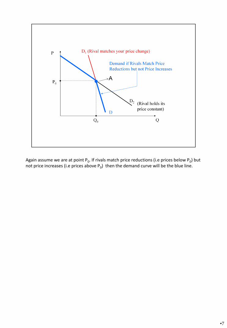
Again assume we are at point P0. If rivals match price reductions (i.e prices below P0) but not price increases (i.e prices above P0) then the demand curve will be the blue line.

•7

The effect of a price reduction on the quantity demanded of your product depends upon whether your rivals respond by cutting their prices too!

The effect of a price increase on the quantity demanded of your product depends upon whether your rivals respond by raising their prices too!

Strategic interdependence: You aren’t in complete control of your own destiny!

•8

The above analysis can be extended to understand the Sweezy model. The Sweezy model is characterized by the following key assumptions:

• Few firms in the market serving many consumers.

• Firms produce differentiated products.

• Barriers to entry.

• Each firm believes rivals will match (or follow) price reductions, but won’t match (or follow) price increases. It is very important to note this assumption of the pricing behavior of the firms. If you deviate from this assumption then the model will not make sense.

•9

The manager in this case believes that the firm will match a price reduction but not a price increase (PLEASE NOTE THAT THE STARTING POINT IS P0), giving us the demand curve in green. So lets analyze this step by step. Take P0 as given and also your starting point. Any price above P0, the demand curve facing the firm is D2. This gives us a relatively elastic demand as rivals are holding price constant. Take a minute to closely look at D2. The shape of the MR curve will be MR2 if demand is D2. If prices are below P0 the demand is D1 and the marginal revenue curve is MR1. Thus, the marginal revenue curve (MR) the firm faces initially is the marginal revenue curve associated with D2 which is MR2; at Q0, it jumps down to the marginal revenue curve corresponding to D1. The final MR is the lime green line!

•10

Profit again is maximized when MR=MC. The output is Q0 and price is P0 at MC1, MC2, MC3. If marginal cost curve jumps up from MC1, only then the output will change.

•11

To summarize:

Firms believe rivals match price cuts, but not price increases.

Firms operating in a Sweezy oligopoly maximize profit by producing where MRS = MC.

The kinked-shaped marginal revenue curve implies that there exists a range over which changes in MC will not impact the profit-maximizing level of output. Therefore, the firm may have no incentive to change price provided that marginal cost remains in a given range.

•12

Lets break for Task 7.1.

•13

Key assumptions of the Cournot model are as follows:

• A few firms produce goods that are perfect substitutes (homogeneous) products.

• Firms’ control variable is output in contrast to price.

• Each firm believes their rivals will hold output constant if it changes its own output (The output of rivals is viewed as given or “fixed”). Another way to think about this is that each firm decides how much to produce at the same time. So essentially both firms have no opportunity to change output levels after observing their rival's behavior.

• Barriers to entry exist.

•14

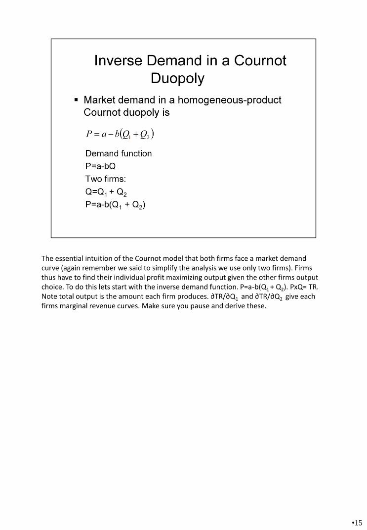
The essential intuition of the Cournot model that both firms face a market demand curve (again remember we said to simplify the analysis we use only two firms). Firms thus have to find their individual profit maximizing output given the other firms output choice. To do this lets start with the inverse demand function. P=a-b(Q1 + Q2). PxQ= TR. Note total output is the amount each firm produces. ∂TR/∂Q1 and ∂TR/∂Q2 give each firms marginal revenue curves. Make sure you pause and derive these.

•15

Marginal revenue of Firm 1 is derived in the above slide

•16

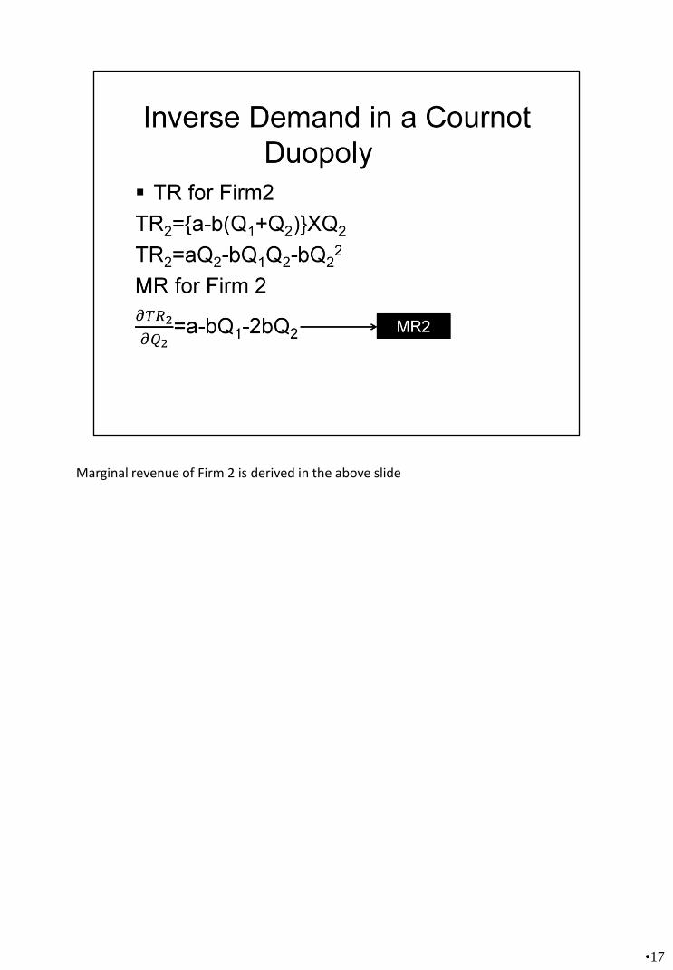
Marginal revenue of Firm 2 is derived in the above slide

•17

•18

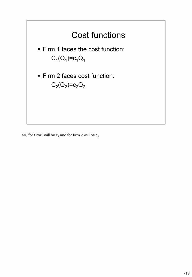
MC for firm1 will be c1 and for firm 2 will be c2

•19

•20

Best-Response function:

• Since a firm’s marginal revenue in a homogeneous Cournot oligopoly depends on both its output and its rivals, each firm needs a way to “respond” to rival’s output decisions.

• Firm 1’s best-response (or reaction) function is a schedule summarizing the amount of Q1 firm 1 should produce in order to maximize its profits for each quantity of Q2 produced by firm 2.

• Since the products are substitutes, an increase in firm 2’s output leads to a decrease in the profit-maximizing amount of firm 1’s product.

•21

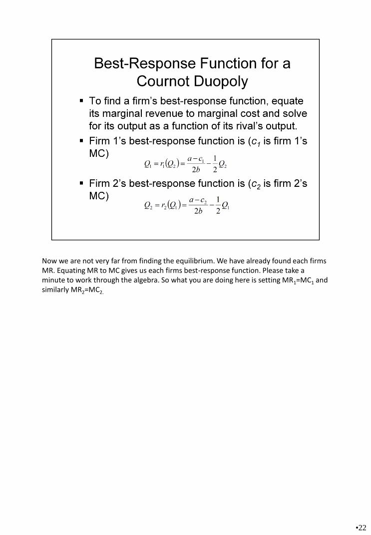
Now we are not very far from finding the equilibrium. We have already found each firms MR. Equating MR to MC gives us each firms best-response function. Please take a minute to work through the algebra. So what you are doing here is setting MR1=MC1 and similarly MR2=MC2.

•22

Using the above equation we can plot each firms response function. In the above case we are plotting Firm 1’s response function. The response function is downward sloping and it simply says that firm 1 output will increase as firm 2 reduces its output. Firm 1 will produce monopoly output (Q1

M) if Firm 2 produces zero units.

•23

Cournot Equilibrium:

Situation where each firm produces the output that maximizes its profits, given the output of rival firms.

No firm can gain by unilaterally changing its own output to improve its profit. A point where the two firm’s best-response functions intersect.

•24

To find equilibrium we solve each firm’s best response functions simultaneously.

•25

Summary of Cournot Equilibrium:

• The output Q1* maximizes firm 1’s profits, given that firm 2 produces Q2

*.

• The output Q2* maximizes firm 2’s profits, given that firm 1 produces Q1

*.

• Neither firm has an incentive to change its output, given the output of the rival.

• Beliefs are consistent:

-In equilibrium, each firm “thinks” rivals will stick to their current output – and they do!

•26

The Cournot equilibrium will become clearer with the help of an application. Lets break to work through the above Task.

•27

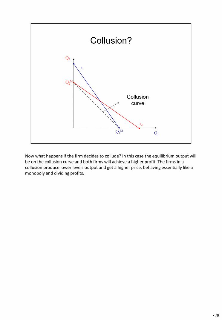
Now what happens if the firm decides to collude? In this case the equilibrium output will be on the collusion curve and both firms will achieve a higher profit. The firms in a collusion produce lower levels output and get a higher price, behaving essentially like a monopoly and dividing profits.

•28

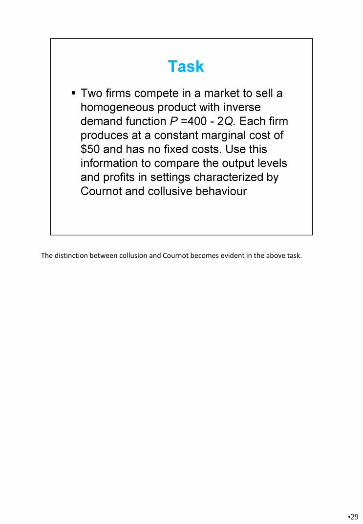
The distinction between collusion and Cournot becomes evident in the above task.

•29

If Firm 1’s marginal cost increases then the response function will change. If Firm 1’s marginal cost increases then the response function will shift down and the new equilibrium will be at Q1

** and Q2**.

•30

•Different oligopoly scenarios give rise to different optimal strategies and different outcomes.

•Your optimal price and output depends on …

Beliefs about the reactions of rivals.

Your choice variable (P or Q) and the nature of the product market (differentiated or homogeneous products).

Your ability to credibly commit prior to your rivals.

•31