Welcome to Managerial Economics, Session 1. Lets begin the first of many exciting sessions in

this course.

1

So today we will be taking an economics perspective on effective management. The main topics

covered are goals and constraints of firms, profits, five forces model, time value of money and

marginal analysis.

2

So what is Managerial economics. Simply put managerial economics gives tools for analyzing

business situations that enables you to become an effective manager. Now effective management

requires a manager. Who is a manager? A manager is a person who directs resources to achieve a

stated goal.

Coming back to the economics part of it. Economics is decision-making under scarcity and

scarcity is having limited resources. Lets take an example, such as time. Coming to lecture

involves the use of your time. Time available to you in a day is a limited resource, it is not

unlimited. Hence, you have to decide whether to attend the lecture or work on an assignment at

home. In other words, you have to give up on something to come to this lecture. Similarly, a

manager has to decide how to allocate scarce resources. If a soft drink company spends a lot on

advertising then it has less resources to spend on product development. Effective management

requires making these choices.

One side point here. Our focus in this course is economic tools required for effective management.

There are other skills needed too like communication skills, a good temperament etc. I don’t deny

this but the scope here is just economics tools.

3

So what kind of tools can we give people to become good managers. To make good decisions,

firstly, a manager must clearly identify goals and constraints. Since resources are limited every

manager faces constraints. For example, as a manager of a restaurant I may want to make my

restaurant the most popular in town and gain the greatest market share. Constraints faced in this

exercise might include not having enough capital to rent a popular location. Thus, in this case I

may have to revise the goal.

4

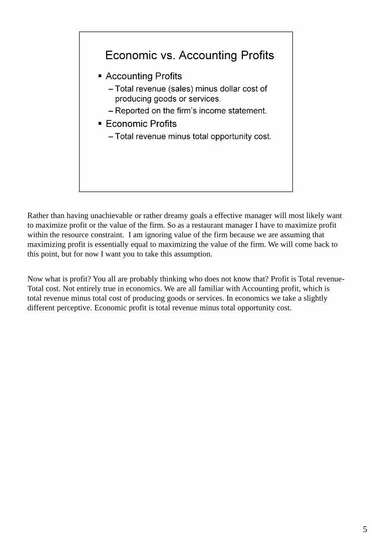
Rather than having unachievable or rather dreamy goals a effective manager will most likely want

to maximize profit or the value of the firm. So as a restaurant manager I have to maximize profit

within the resource constraint. I am ignoring value of the firm because we are assuming that

maximizing profit is essentially equal to maximizing the value of the firm. We will come back to

this point, but for now I want you to take this assumption.

Now what is profit? You all are probably thinking who does not know that? Profit is Total revenue-

Total cost. Not entirely true in economics. We are all familiar with Accounting profit, which is

total revenue minus total cost of producing goods or services. In economics we take a slightly

different perceptive. Economic profit is total revenue minus total opportunity cost.

5

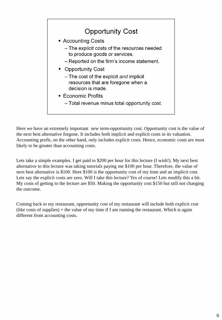
Here we have an extremely important new term-opportunity cost. Opportunity cost is the value of

the next best alternative forgone. It includes both implicit and explicit costs in its valuation.

Accounting profit, on the other hand, only includes explicit costs. Hence, economic costs are most

likely to be greater than accounting costs.

Lets take a simple examples. I get paid to $200 per hour for this lecture (I wish!). My next best

alternative to this lecture was taking tutorials paying me $100 per hour. Therefore, the value of

next best alternative is $100. Here $100 is the opportunity cost of my time and an implicit cost.

Lets say the explicit costs are zero. Will I take this lecture? Yes of course! Lets modify this a bit.

My costs of getting to the lecture are $50. Making the opportunity cost $150 but still not changing

the outcome.

Coming back to my restaurant, opportunity cost of my restaurant will include both explicit cost

(like costs of supplies) + the value of my time if I am running the restaurant. Which is again

different from accounting costs.

6

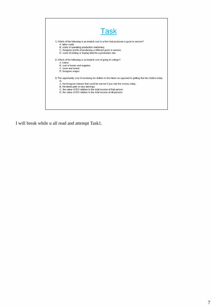
I will break while u all read and attempt Task1.

7

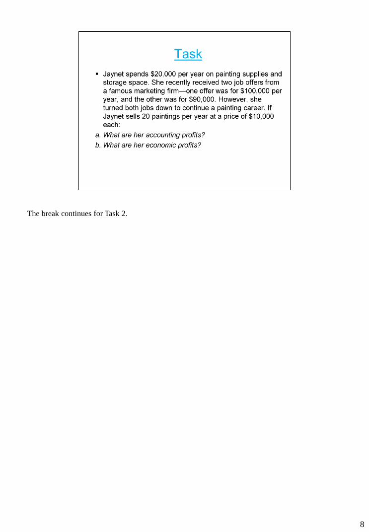
The break continues for Task 2.

8

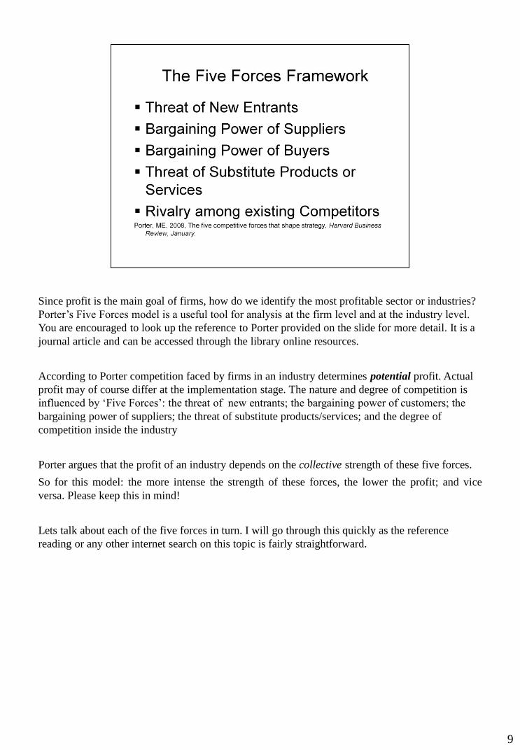
Since profit is the main goal of firms, how do we identify the most profitable sector or industries?

Porter’s Five Forces model is a useful tool for analysis at the firm level and at the industry level.

You are encouraged to look up the reference to Porter provided on the slide for more detail. It is a

journal article and can be accessed through the library online resources.

According to Porter competition faced by firms in an industry determines potential profit. Actual

profit may of course differ at the implementation stage. The nature and degree of competition is

influenced by ‘Five Forces’: the threat of new entrants; the bargaining power of customers; the

bargaining power of suppliers; the threat of substitute products/services; and the degree of

competition inside the industry

Porter argues that the profit of an industry depends on the collective strength of these five forces.

So for this model: the more intense the strength of these forces, the lower the profit; and vice

versa. Please keep this in mind!

Lets talk about each of the five forces in turn. I will go through this quickly as the reference

reading or any other internet search on this topic is fairly straightforward.

9

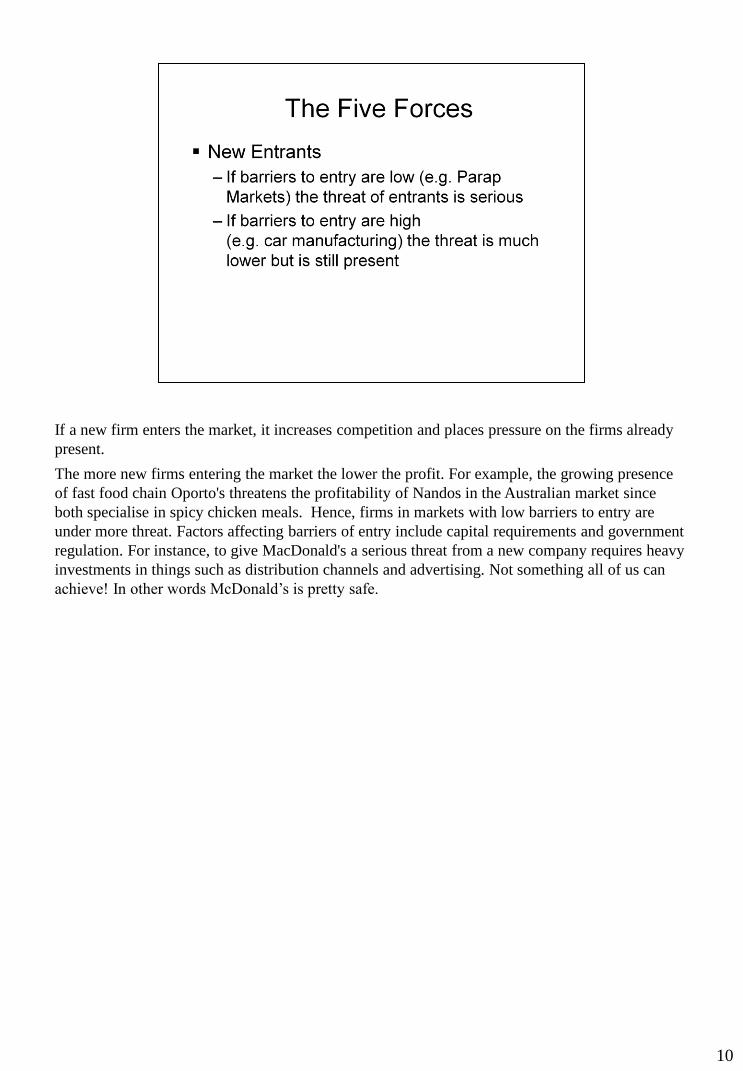
If a new firm enters the market, it increases competition and places pressure on the firms already

present.

The more new firms entering the market the lower the profit. For example, the growing presence

of fast food chain Oporto's threatens the profitability of Nandos in the Australian market since

both specialise in spicy chicken meals. Hence, firms in markets with low barriers to entry are

under more threat. Factors affecting barriers of entry include capital requirements and government

regulation. For instance, to give MacDonald's a serious threat from a new company requires heavy

investments in things such as distribution channels and advertising. Not something all of us can

achieve! In other words McDonald’s is pretty safe.

10

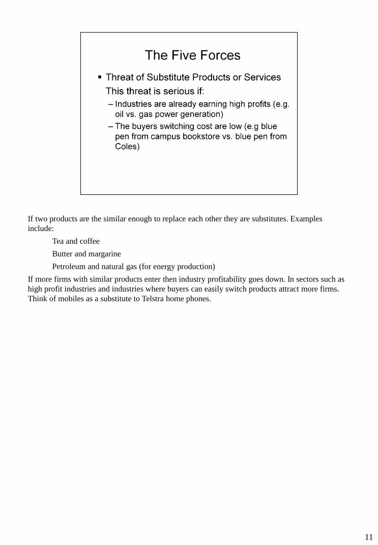
If two products are the similar enough to replace each other they are substitutes. Examples

include:

Tea and coffee

Butter and margarine

Petroleum and natural gas (for energy production)

If more firms with similar products enter then industry profitability goes down. In sectors such as

high profit industries and industries where buyers can easily switch products attract more firms.

Think of mobiles as a substitute to Telstra home phones.

11

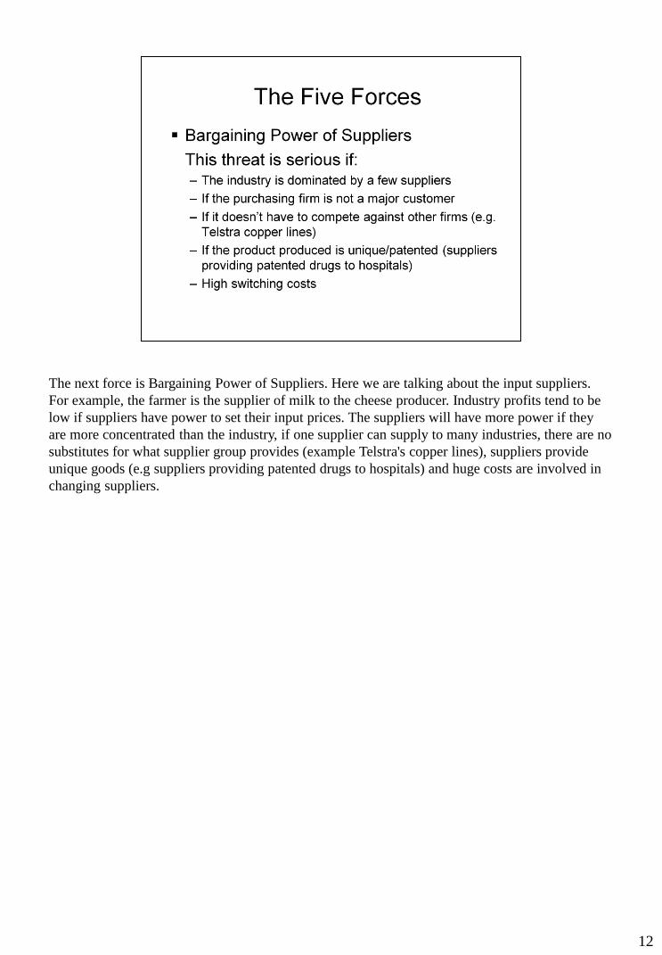
The next force is Bargaining Power of Suppliers. Here we are talking about the input suppliers.

For example, the farmer is the supplier of milk to the cheese producer. Industry profits tend to be

low if suppliers have power to set their input prices. The suppliers will have more power if they

are more concentrated than the industry, if one supplier can supply to many industries, there are no

substitutes for what supplier group provides (example Telstra's copper lines), suppliers provide

unique goods (e.g suppliers providing patented drugs to hospitals) and huge costs are involved in

changing suppliers.

12

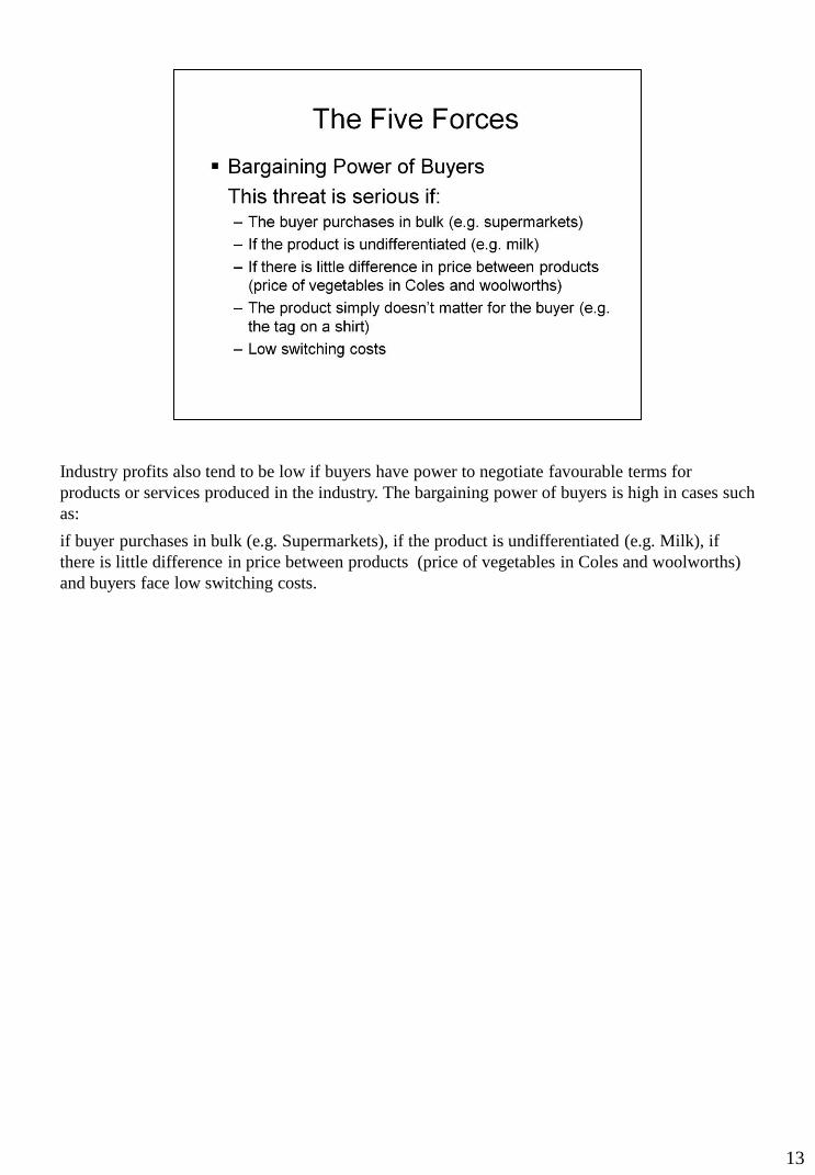
Industry profits also tend to be low if buyers have power to negotiate favourable terms for

products or services produced in the industry. The bargaining power of buyers is high in cases such

as:

if buyer purchases in bulk (e.g. Supermarkets), if the product is undifferentiated (e.g. Milk), if

there is little difference in price between products (price of vegetables in Coles and woolworths)

and buyers face low switching costs.

13

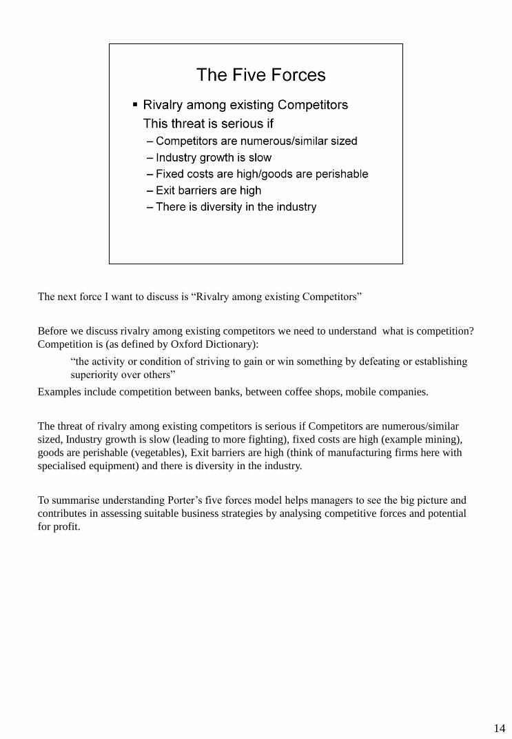
The next force I want to discuss is “Rivalry among existing Competitors”

Before we discuss rivalry among existing competitors we need to understand what is competition?

Competition is (as defined by Oxford Dictionary):

“the activity or condition of striving to gain or win something by defeating or establishing

superiority over others”

Examples include competition between banks, between coffee shops, mobile companies.

The threat of rivalry among existing competitors is serious if Competitors are numerous/similar

sized, Industry growth is slow (leading to more fighting), fixed costs are high (example mining),

goods are perishable (vegetables), Exit barriers are high (think of manufacturing firms here with

specialised equipment) and there is diversity in the industry.

To summarise understanding Porter’s five forces model helps managers to see the big picture and

contributes in assessing suitable business strategies by analysing competitive forces and potential

for profit.

14

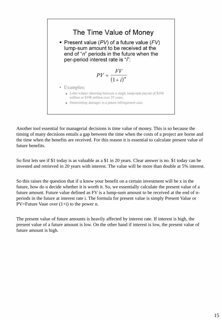
Another tool essential for managerial decisions is time value of money. This is so because the

timing of many decisions entails a gap between the time when the costs of a project are borne and

the time when the benefits are received. For this reason it is essential to calculate present value of

future benefits.

So first lets see if $1 today is as valuable as a $1 in 20 years. Clear answer is no. $1 today can be

invested and retrieved in 20 years with interest. The value will be more than double at 5% interest.

So this raises the question that if u know your benefit on a certain investment will be x in the

future, how do u decide whether it is worth it. So, we essentially calculate the present value of a

future amount. Future value defined as FV is a lump-sum amount to be received at the end of n-

periods in the future at interest rate i. The formula for present value is simply Present Value or

PV=Future Vaue over (1+i) to the power n.

The present value of future amounts is heavily affected by interest rate. If interest is high, the

present value of a future amount is low. On the other hand if interest is low, the present value of

future amount is high.

15

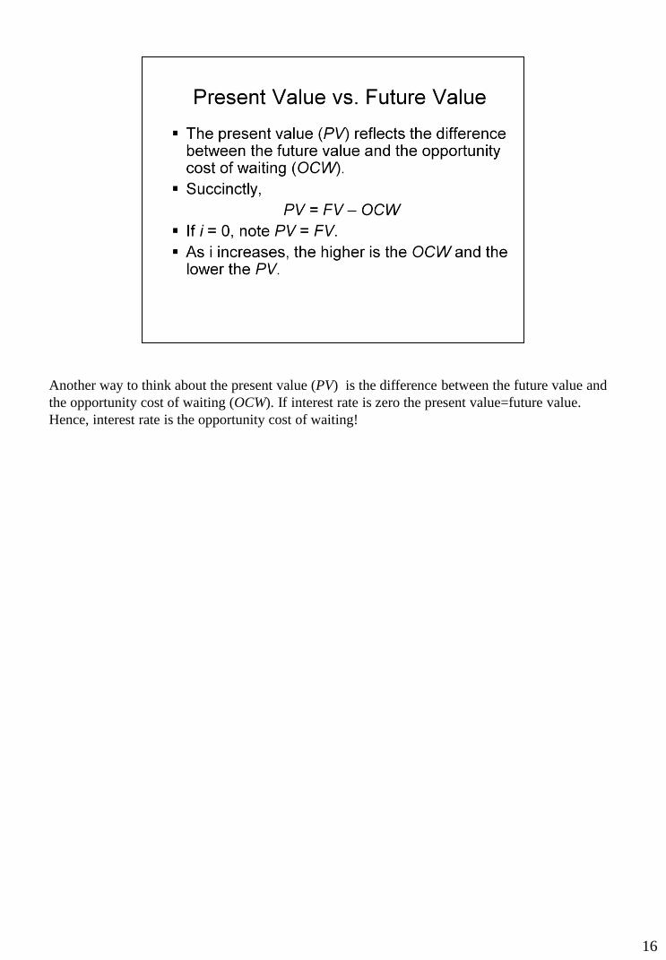
Another way to think about the present value (PV) is the difference between the future value and

the opportunity cost of waiting (OCW). If interest rate is zero the present value=future value.

Hence, interest rate is the opportunity cost of waiting!

16

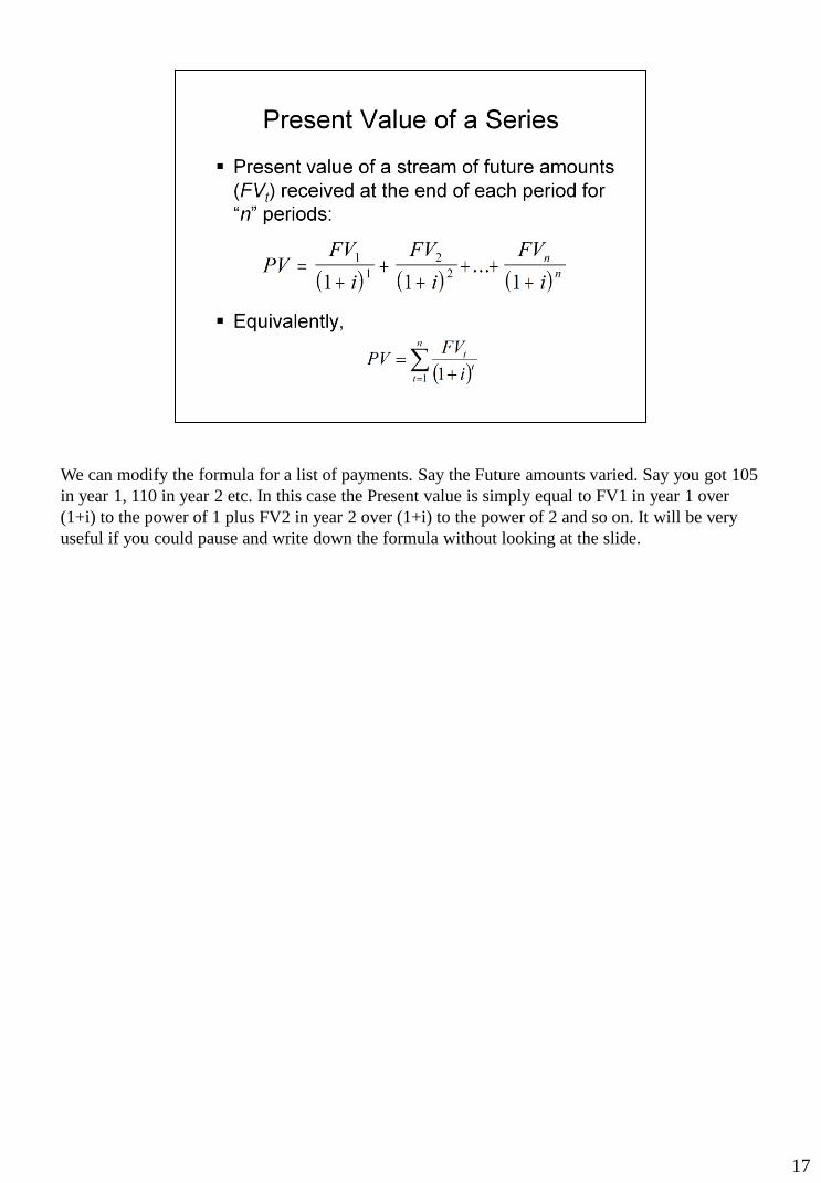
We can modify the formula for a list of payments. Say the Future amounts varied. Say you got 105

in year 1, 110 in year 2 etc. In this case the Present value is simply equal to FV1 in year 1 over

(1+i) to the power of 1 plus FV2 in year 2 over (1+i) to the power of 2 and so on. It will be very

useful if you could pause and write down the formula without looking at the slide.

17

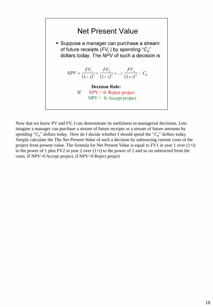
Now that we know PV and FV, I can demonstrate its usefulness in managerial decisions. Lets

imagine a manager can purchase a stream of future receipts or a stream of future amounts by

spending “C0” dollars today. How do I decide whether I should spend the “C0” dollars today.

Simply calculate the The Net Present Value of such a decision by subtracting current costs of the

project from present value. The formula for Net Present Value is equal to FV1 in year 1 over (1+i)

to the power of 1 plus FV2 in year 2 over (1+i) to the power of 2 and so on subtracted from the

costs. If NPV>0 Accept project, if NPV<0 Reject project

18

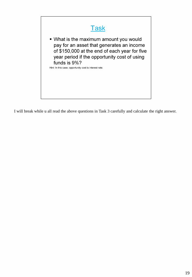
I will break while u all read the above questions in Task 3 carefully and calculate the right answer.

19

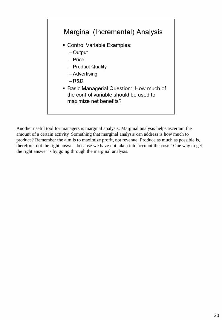
Another useful tool for managers is marginal analysis. Marginal analysis helps ascertain the

amount of a certain activity. Something that marginal analysis can address is how much to

produce? Remember the aim is to maximize profit, not revenue. Produce as much as possible is,

therefore, not the right answer- because we have not taken into account the costs! One way to get

the right answer is by going through the marginal analysis.

20

Before we get into marginal analysis lets revisit the issue of profit. Lets think of economic profit

here which is total revenue minus opportunity cost. We can capture this idea in general terms and

express this as net benefits= total benefits minus total costs. Total costs can be opportunity of cost

of production and total benefits can be revenue arising from sale of q items or p*q. The formula of

net benefits can also be applied in other contexts.

21

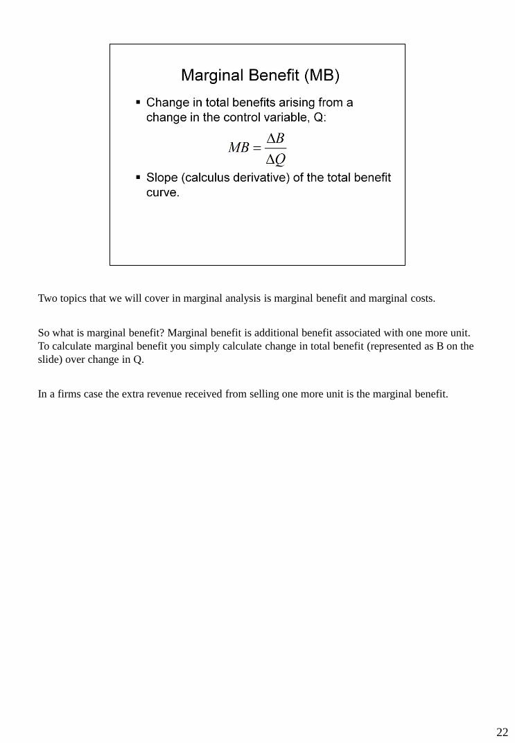
Two topics that we will cover in marginal analysis is marginal benefit and marginal costs.

So what is marginal benefit? Marginal benefit is additional benefit associated with one more unit.

To calculate marginal benefit you simply calculate change in total benefit (represented as B on the

slide) over change in Q.

In a firms case the extra revenue received from selling one more unit is the marginal benefit.

22

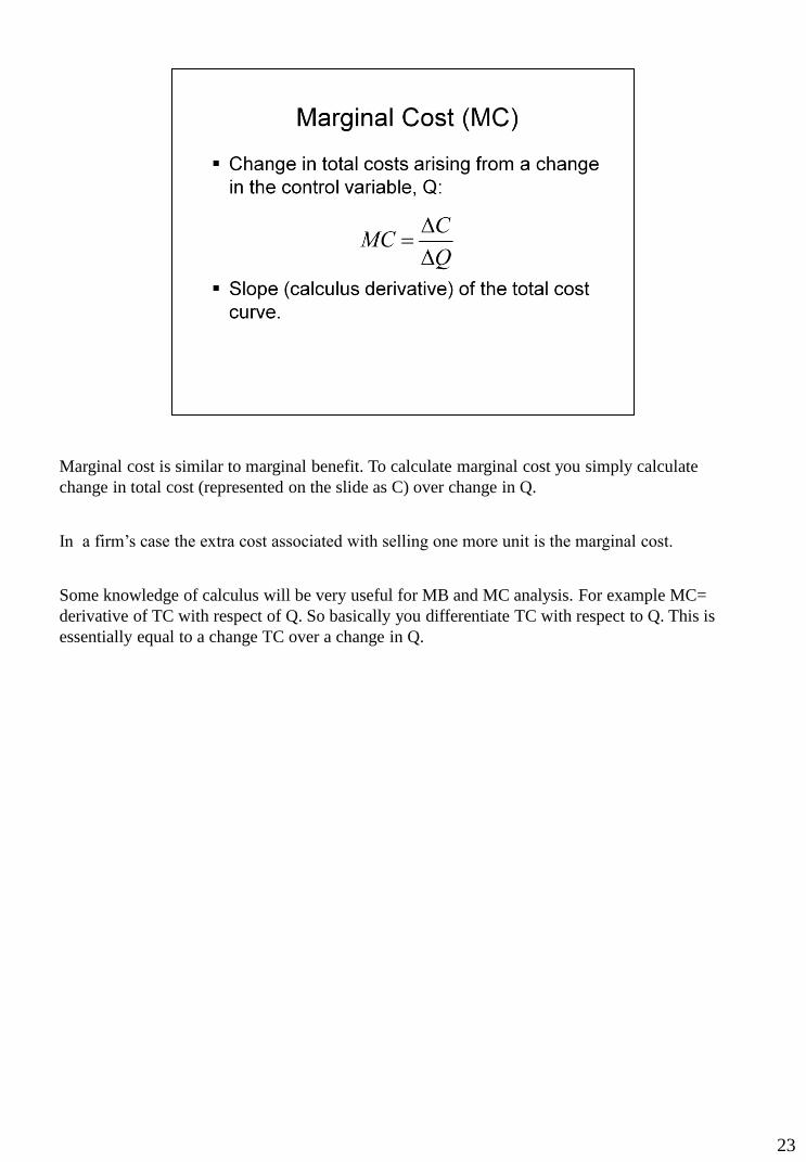
Marginal cost is similar to marginal benefit. To calculate marginal cost you simply calculate

change in total cost (represented on the slide as C) over change in Q.

In a firm’s case the extra cost associated with selling one more unit is the marginal cost.

Some knowledge of calculus will be very useful for MB and MC analysis. For example MC=

derivative of TC with respect of Q. So basically you differentiate TC with respect to Q. This is

essentially equal to a change TC over a change in Q.

23

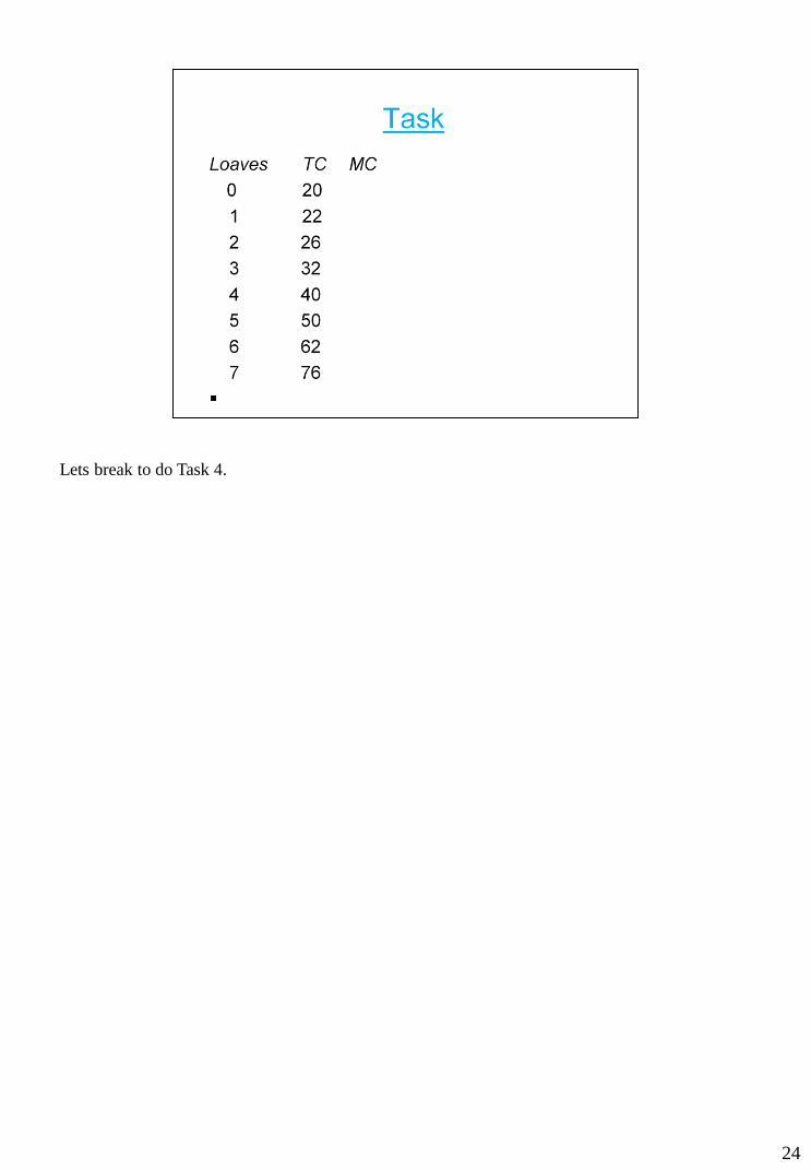
Lets break to do Task 4.

24

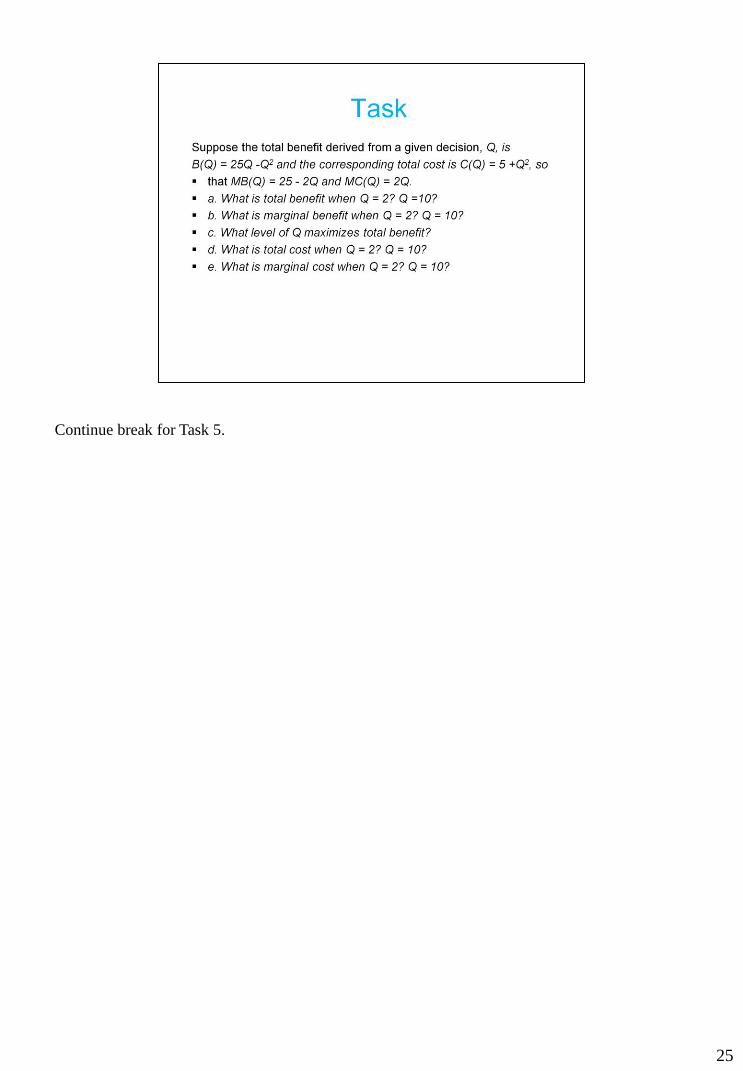
Continue break for Task 5.

25

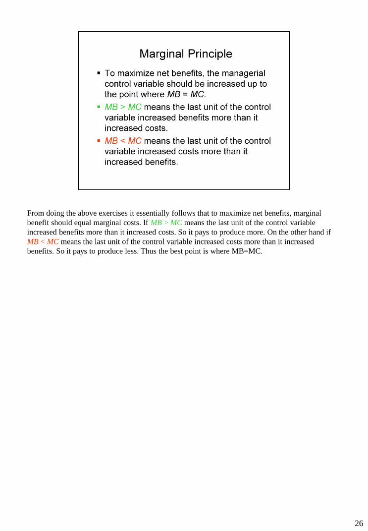
From doing the above exercises it essentially follows that to maximize net benefits, marginal

benefit should equal marginal costs. If MB > MC means the last unit of the control variable

increased benefits more than it increased costs. So it pays to produce more. On the other hand if

MB < MC means the last unit of the control variable increased costs more than it increased

benefits. So it pays to produce less. Thus the best point is where MB=MC.

26

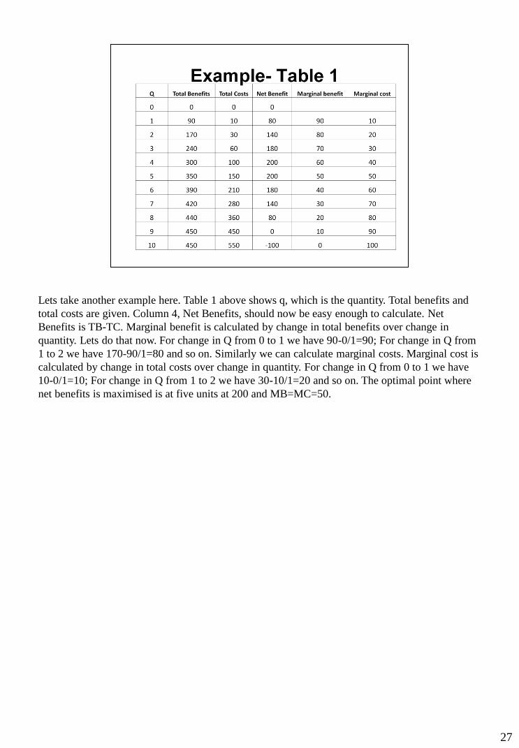
Lets take another example here. Table 1 above shows q, which is the quantity. Total benefits and

total costs are given. Column 4, Net Benefits, should now be easy enough to calculate. Net

Benefits is TB-TC. Marginal benefit is calculated by change in total benefits over change in

quantity. Lets do that now. For change in Q from 0 to 1 we have 90-0/1=90; For change in Q from

1 to 2 we have 170-90/1=80 and so on. Similarly we can calculate marginal costs. Marginal cost is

calculated by change in total costs over change in quantity. For change in Q from 0 to 1 we have

10-0/1=10; For change in Q from 1 to 2 we have 30-10/1=20 and so on. The optimal point where

net benefits is maximised is at five units at 200 and MB=MC=50.

27

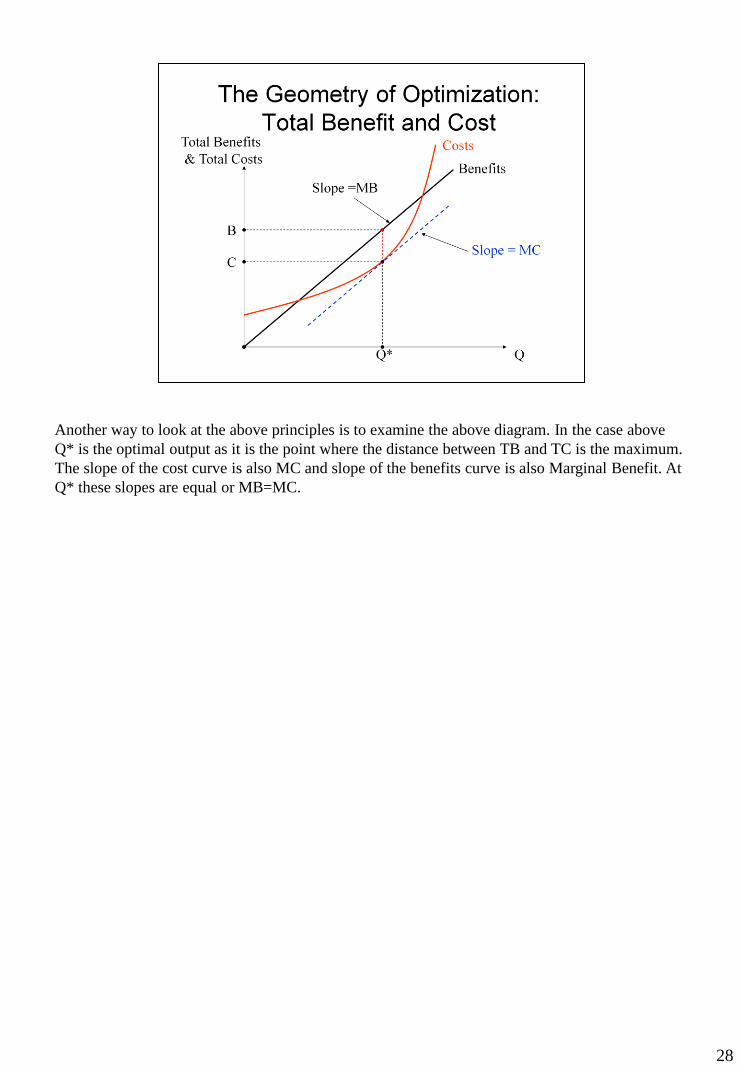
Another way to look at the above principles is to examine the above diagram. In the case above

Q* is the optimal output as it is the point where the distance between TB and TC is the maximum.

The slope of the cost curve is also MC and slope of the benefits curve is also Marginal Benefit. At

Q* these slopes are equal or MB=MC.

28

To summarize, an effective manager is careful to include:

all costs and benefits when making decisions. And calculate the costs using the opportunity cost

method.

Recognizes time value of money

And optimizes uses marginal analysis

29