Wei Prater
51
1' If- The Structure and Analysis of Complex Reaction Systems JAMES WEI AND CHARLES D. PRATER Socony Mobil Oil Co., Inc., Research Department, Paulsboro, New Jersey Page I. Introduction 204 II. Reversible Monomolecular Systems 208 A. The Rate Equations for Reversible Monomolecular Systems 208 yB. The Geometry of the System 213 yC. The Structure of Reversible Monomolecular Systems 243 III. The Determination of the Values of the Rate Constants for Typical Reversi- ble Monomolecular Systems Using the Characteristic Directions 244 ^A. The Treatment of Experimental Data 244 •/B. Example of a Three Component System: Butene Isomerization over Pure , Alumina Catalyst 247 •if f vTj, An Example of a Pour Component System 257 IV. Irreversible Monomolecular Systems 270 -"«•••» A. Geometric Properties of Irreversible Systems 270 B. Experimental Procedures for the Determination of Rate Constants from Characteristic Directions for Irreversible Systems and Applications to Typical Examples 285 V. Miscellaneous Topics Concerning Monomolecular Systems 295 vA.. Location of- Maxima and Minima in the Amounts of Various Species.... 295 B. Perturbations on the Rate Constant Matrix 302 C. Insensitivity of Single Curved Reaction Paths to the Values of the Rate Constants - - . . - 309 VI. Pseudo-Mass-Action Systems in Heterogeneous Catalysis 313 A. Some Classes of Heterogeneous Catalytic Reaction Systems with Rate Equations of the Pseudomonomolecular and Pseudo-Mass-Action Form. 313 B. Systems with more than a Single Type of Independent Catalytic Site... 332 C. The Hydrogenation-dehydrogenation of C 6 -Cyclics over Supported Plati- num Catalyst as a Pseudo-Mass-Action System 334 VII. Qualitative Features of General Complex Reaction Systems 339 A. General Comments 339 B. Constraints 340 C. The Equilibrium Point in General Complex Reaction Systems 343 D. Liapounov Functions 344 E. Irreversible Thermodynamics and the Relation of Liapounov Functions to the Direction of the Reaction Paths 349 VIII. General Discussion and Literature Survey 355 /i. APPENDICES The Orthogonal Characteristic System 364 A. Transformation of the Rate Constant Matrix into a Symmetric Matrix. 364 B. Transformation to the Orthogonal Characteristic Coordinate System — 368 203
-
Upload
maquiman-kiyama -
Category
Documents
-
view
329 -
download
13
Transcript of Wei Prater
1 ' I f -
The Structure a n d Ana lys i s o f C o m p l e x React ion Systems
JAMES WEI AND CHARLES D. PRATER
Socony Mobil Oil Co., Inc., Research Department, Paulsboro, New Jersey
Page I. Introduction 204
II. Reversible Monomolecular Systems 208 A. The Rate Equations for Reversible Monomolecular Systems 208
yB. The Geometry of the System 213 yC. The Structure of Reversible Monomolecular Systems 243
III. The Determination of the Values of the Rate Constants for Typical Reversible Monomolecular Systems Using the Characteristic Directions 244
^A. The Treatment of Experimental Data 244 •/B. Example of a Three Component System: Butene Isomerization over Pure
, Alumina Catalyst 247 •if f vTj, An Example of a Pour Component System 257
IV. Irreversible Monomolecular Systems 270 -"«•••» A. Geometric Properties of Irreversible Systems 270
B. Experimental Procedures for the Determination of Rate Constants from Characteristic Directions for Irreversible Systems and Applications to Typical Examples 285
V. Miscellaneous Topics Concerning Monomolecular Systems 295 vA.. Location of- Maxima and Minima in the Amounts of Various Species.... 295
B. Perturbations on the Rate Constant Matrix 302 C. Insensitivity of Single Curved Reaction Paths to the Values of the Rate
Constants - - . . - 309 VI. Pseudo-Mass-Action Systems in Heterogeneous Catalysis 313
A. Some Classes of Heterogeneous Catalytic Reaction Systems with Rate Equations of the Pseudomonomolecular and Pseudo-Mass-Action Form. 313
B. Systems with more than a Single Type of Independent Catalytic Site... 332 C. The Hydrogenation-dehydrogenation of C6-Cyclics over Supported Plati
num Catalyst as a Pseudo-Mass-Action System 334 VII. Qualitative Features of General Complex Reaction Systems 339
A. General Comments 339 B. Constraints 340 C. The Equilibrium Point in General Complex Reaction Systems 343 D. Liapounov Functions 344 E. Irreversible Thermodynamics and the Relation of Liapounov Functions to
the Direction of the Reaction Paths 349 VIII. General Discussion and Literature Survey 355
/ i .
APPENDICES The Orthogonal Characteristic System 364 A. Transformation of the Rate Constant Matrix into a Symmetric Matrix. 364 B. Transformation to the Orthogonal Characteristic Coordinate System — 368
203
204 JAMES WEI AND CHARLES D. PRATER
C. Proof That the Characteristic Roots of the Rate Constant Matrix K are Nonpositive Real Numbers 370
D. The Calculation of the Inverse Matrix X-1 371 II. Explicit Solution for the General Three Component System 372
III. A Convenient Method for Computing the Characteristic Vectors and Roots of the Rate Constant Matrix K 376
IV. Canonical Forms ? 330 V. List of Symbols 381
References 390
I. Introduction
In catalytic and enzyme chemistry we often encounter highly coupled systems of chemical reactions involving several chemical species.,IUis_am important .purpose_ofaehemical* kinetics^to~explore"aiid -to.descr.be nthe rela-r
tiqnsjjet.w„eenjhe__amjooin^
r^cti^i^ajid^oirelateithejconcentrationj^hanges.to aiminimal.numfeei^of concentration. indep.endentrparameters.that. characterize- the Treact,ion_R_v^ tem. Reaction kinetics provide an important part of the understanding of highly coupled systems and, in addition, provide the method for predicting their behavior. As is well known from previous attempts, the behavior of even linear systems containing as few as three reacting species is sufficiently complicated to make their basic dynamic behavior difficult to visualize.
Chemical kinetics also plays a basic role in the study of the nature of catalytic activity. Studies of the catalyst and reactants in the absence of appreciable over-all reaction, such as studies of the electronic properties of catalytic solids or optical studies of adsorbed molecular species can provide valuable information about these materials. In most cases, however, kinetic data are ultimately needed to establish the relation and relevance of any information derived from such studies to the catalytic reaction itself. For example, a particular adsorbed species may be observed and studied by a spectral technique; yet it need not play any essential role in the catalytic reaction since adsorption is a more general phenomenon than catalytic activity. On the other hand, kinetics studies can provide information about the variation, as a function of experimental conditions, of the relative number of adsorbed species that play a basic role in the reaction. Consequently, such information may make it possible to identify which, if any, of the adsorbed species studied by the use of a direct analytical technique are relevant to the reaction. As another example, when studies are made of the solid state properties of a given catalytic solid, the question as to which, if any, of these properties are related to catalytic activity must ultimately be answered in terms of consistency with the observed behavior of the reaction system.
ANALYSIS OF COMPLEX REACTION SYSTEMS 205
The information needed about the chemical kinetics of a reaction system is best determined in terms of the structure of general classes of such systems. By structure we mean qualitative and quantitative features that are common to large well-defined classes of systems. For the classes of complex reaction systems to be discussed in detail in this article, the structural approach leads to two related but independent results. First, descriptive models and analyses are developed that create a sound basis for understanding the macroscopic behavior of complex as well as simple dynamic systems. Second, these descriptive models and the procedures obtained from them lead to a new and powerful method for determining the rate parameters from experimental data. The structural analysis is best approached by a geometrical interpretation of the behavior of the reaction system. Such a description can be readily visualized.
The structural approach will also contribute to the analysis of the thermodynamics of nonequilibrium systems. It is the aim and purpose of thermodynamics to describe structural features of systems in terms of macroscopic variables. Unfortunately, classical thermodynamics is concerned almost entirely with the equilibrium state; it makes only weak statements about nonequilibrium systems. The nonequilibrium thermodynamics of Onsager (1), Prigogine (2), and others introduces additional axioms into classical thermodynamics in an attempt to obtain stronger and more useful statements about nonequilibrium systems. These axioms lead, however, to an expression for the driving force of chemical reactions that does not agree with experience and that is only applicable, as an approximation, to small departures from equilibrium. A way in which this situation may be improved is outlined in Section VII.
The major part of this article will be devoted to a particular class of reac-tion systems-—namely, monomolecular systems.TATre^tioirsys^emj3f.j7rO nwlecular-species^is.ca^led^onom pair_of.spe"ries_'is"bT first'ortler,reactions.only? These linear systems are satisfactory representations for many rate processes over the entire range of reaction and are linear approximations for most systems in a sufficiently small range. They play a role in the chemical kinetics of complex systems somewhat analogous to the role played by the equation of state of a perfect gas in classical thermodynamics. Consequently, an understanding of their behavior is a prerequisite for the study of more general systems.
Two subclasses of monomolecular systems will be discussed: reversible and irreversible monomolecular systems. A reaction system will be called reversible monomolecular if the coupling between species is by reversible first order reactions only. A typical example of a reversible monomolecular system is
h
206 JAMES WEI AND CHARLES D. PRATER
a ) •A,
where the zth molecular species is designated A*. A reaction system will be called irreversibly monomolecular if some of the species are connected to other species by first order reactions that are irreversible. The presence of completely irreversible steps implies an infinite change in free energy and is consequently ah idealization. Nevertheless, many reactions contain steps with a sufficiently large change in free energy so that irreversibility is an excellent approximation for them except in the neighborhood of the equilibrium point.
The typo of approach to be used and its advantage over the conventional approach is illustrated in Section II,A by a brief discussion of the problem of determining the value of the rate constants from experimental data-for reversible monomolecular systems.
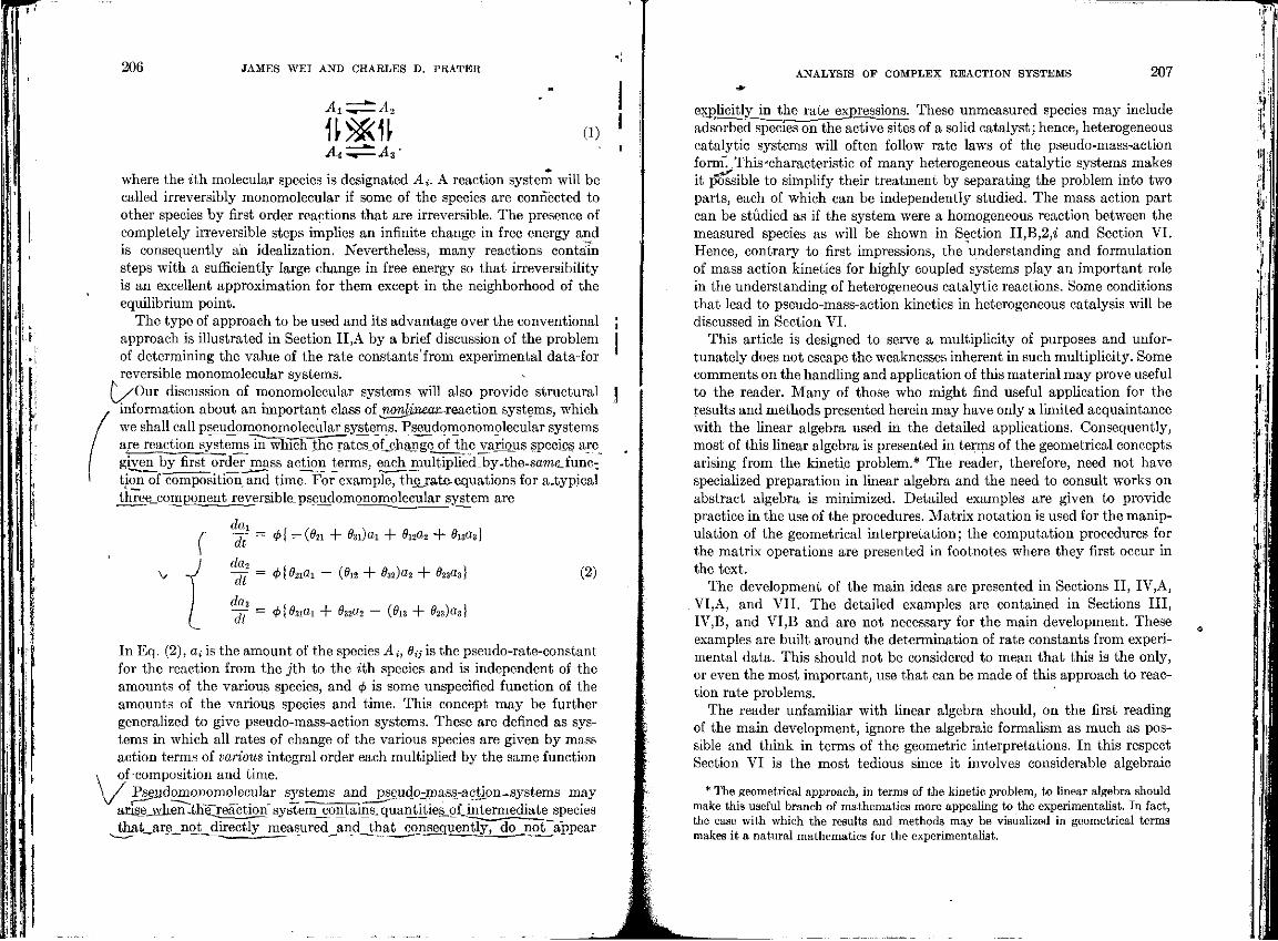
Our discussion of monomolecular systems will also provide structural information about an important class of wonji-aeaji-reaction systems, which we shall call pseudomonomolecular systems. Pseudomonomolecular systems are reaction systems in wliich the rates .oLchange of the various species are giyen_by first order mass action terms, each multipUed_by.the-same.func-tion of composition and time. For example, thejate-equations for a.typical three_component reversible, pseudomonomolecular system are
/.
v
dax
It da2
dt
rffl. dt
= 4>[ -(02i + 0_i)a_ + ta! + $ua>
= 4>&2iai - (0i2 + 6*32)02 + #»a_
= <f>82iai + e32a2 - (0i3 + 023)03
(2)
In Eq. (2), a. is the amount of the species A., 0,-,- is the pseudo-rate-constant for the reaction from the jfh to the iih species and is independent of the amounts of the various species, and <j> is some unspecified function of the amounts of the various species and time. This concept may be further generalized to give pseudo-mass-action systems. These are defined as systems in which all rates of change of the various species are given by mass action terms of various integral order each multiplied by the same function
Vofcomposition and time.
Pseudomonomolecular systems and pseudo-mass-action-systems may anse____hen-theZreaction sysTem^contams.quanj^ies_gf_mtermediate species that__are_not directly measured _and^hatcojose^u^t ly ! do_not appear
ANALYSIS OF COMPLEX REACTION SYSTEMS 207
explicitly in the rate expressions. These unmeasured species may include adsorbed species on the active sites of a solid catalyst; hence, heterogeneous catalytic systems will often follow rate laws of the pseudo-mass-action form. .This'characteristic of many heterogeneous catalytic systems makes it p'ossible to simplify their treatment by separating the problem into two parts, each of which can be independently studied. The mass action part can be studied as if the system were a homogeneous reaction between the measured species as will be shown in Section II,B,2,« and Section VI. Hence, contrary to first impressions, the understanding and formulation of mass action kinetics for highly coupled systems play an important role in the understanding of heterogeneous catalytic reactions. Some conditions that lead to pseudo-mass-action kinetics in heterogeneous catalysis will be discussed in Section VI.
This article is designed to serve a multiplicity of purposes and unfortunately does not escape the weaknesses inherent in such multiplicity. Some comments on the handling and application of this material may prove useful to the reader. Many of those who might find useful application for the results and methods presented herein may have only a limited acquaintance with the linear algebra used in the detailed applications. Consequently, most of this linear algebra is presented in terms of the geometrical concepts arising from the kinetic problem.* The reader, therefore, need not have specialized preparation in linear algebra and the need to consult works on abstract algebra is minimized. Detailed examples are given to provide practice in the use of the procedures. Matrix notation is used for the manipulation of the geometrical interpretation; the computation procedures for the matrix operations are presented in footnotes where they first occur in the text.
The development of the main ideas are presented in Sections II, IV,A, VI,A, and VII. The detailed examples are contained in Sections III, IV,B, and VI,B and are not necessary for the main development. These examples are built around the determination of rate constants from experimental data. This should not be considered to mean that this is the only, or even the most important, use that can be made of this approach to reaction rate problems.
The reader unfamiliar with linear algebra should, on the first reading of the main development, ignore the algebraic formalism as much as possible and think in terms of the geometric interpretations. In this respect Section VI is the most tedious since it involves considerable algebraic
* The geometrical approach, in terms of the kinetic problem, to linear algebra should make this useful branch of mathematics more appealing to the experimentalist. In fact, the ease with which the results and methods may be visualized in geometrical terms makes it a natural mathematics for the experimentalist.
fl
208 JAMES WEI AND CHARLES D. PRATER
manipulation. This section is, however, of importance to the investigator in heterogeneous catalysis.
The reader familiar with linear algebra may obtain the main points of the development from Section II,A, Section II,B,2,c,d,e,o,j, Section II,C, Appendix I, Section IV,A, Section VI,A, and Section VII. -
The relation of the results of previous investigations to the results presented in this article is best understood against a background of the complete picture. I t is for this reason that few references to previous work will be given before Section VIII, which contains a historical survey and a discussion of the relations of previous results to the results presented in this article.
V , il. Reversible Monomolecular Systems
A. T H E RATE EQUATIONS FOR REVERSIBLE MONOMOLECULAR SYSTEMS
1. The General Solution
Let the tth species of a monomolecular reaction system be designated by A. and the amount by a*-. Let the rate constant for the reaction of the
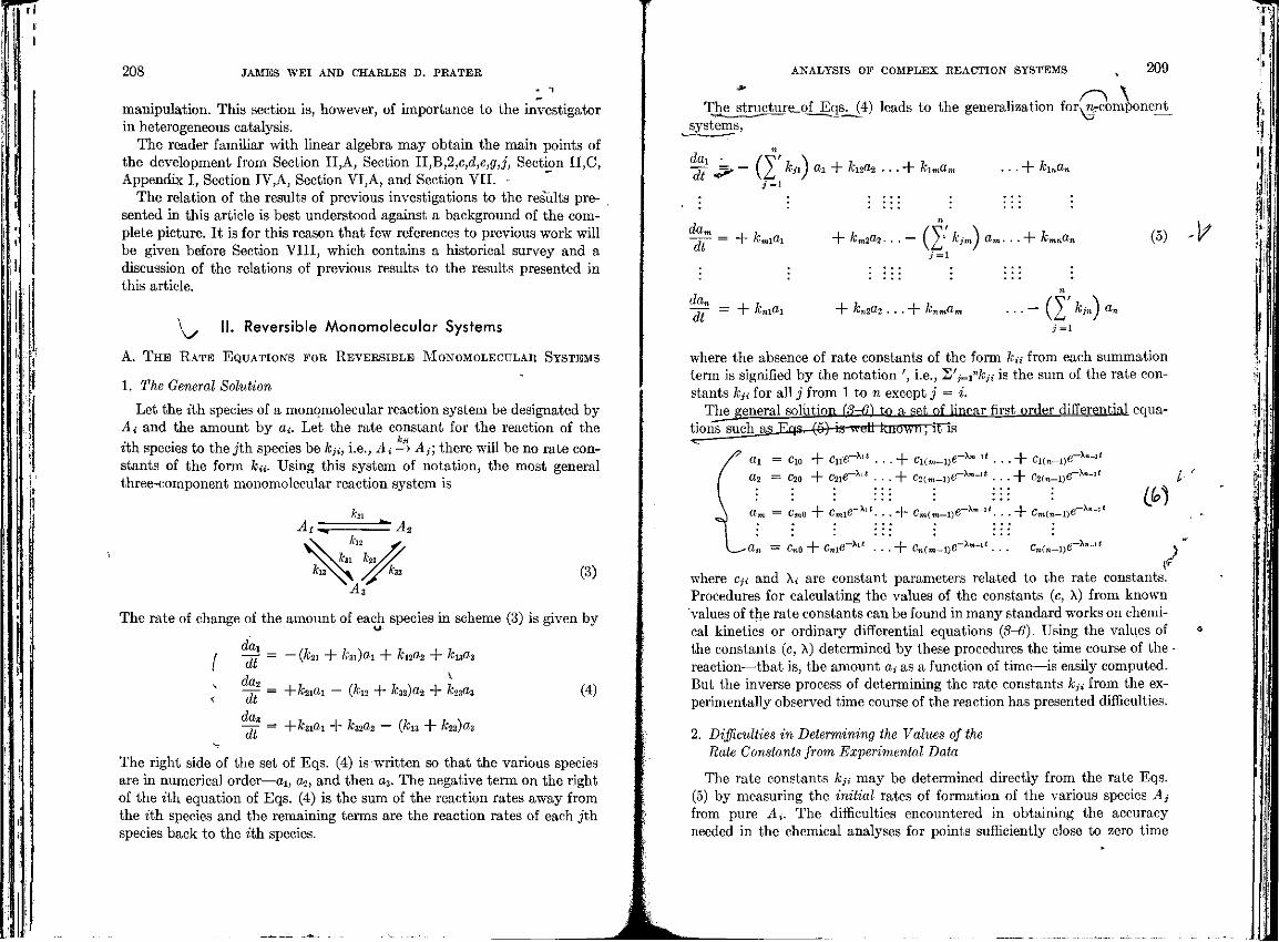
kji iih. species to thej'th species be kji, i.e., Ai —> A,-; there will be no rate constants of the form _c«. Using this system of notation, the most general three-component monomolecular reaction system is
AiZZ
(3)
The rate of change of the amount of each species in scheme (3) is given by
da\ -jT = - (hi + ^3i)ai + kna2 + k13a3
-TT = +^2101 - (&12 + M«2 + fatfH
-j7 = +^31^1 + kna2 — (ku + ft»)a3
(4)
The right side of the set of Eqs. (4) is written so that the various species are in numerical order—a_, a2, and then a3. The negative term on the right of the -th equation of Eqs. (4) is the sum of the reaction rates away from the tth species and the remaining terms are the reaction rates of each jth species back to the ith species.
ANALYSIS OF COMPLEX REACTION SYSTEMS 209
npc TTie_structoe_of^qs_;_(4) leads to the generalization for^rcomponent_ systems,
dai ~dt ^
n =, — ( kfl) Oi + kna% . . . + klmam . . . + kinan
3=1
dt (5)
. =1
dan
w = -r kniai
n
+ kn2a2 . . .+ knnAm • • • — ( ^ kjn) «* J=l
where the absence of rate constants of the form ku from each summation term is signified by the notation ', i.e., __.';-__i"fcji is the sum of the rate constants k^ for all j from 1 to n except j = i.
Thejreneral solution (8-6 to n. set of linear first order differential equations such aa_Eai»*- (5) iu. wull~ known; i r i s
ai = Cio + cne~M . . . + ci(m^i)e-x™-,( . . . + ci<«_-i)e Xn-,(
a2 = c20 + c2ie~Xlf . . . + C2(m_i)e^x"*-1' . . . + C2(7.__)e_x"-lt
a™ = cm0 + cmle-Xl ' . . . + c™m_i)e-Xm-1'. . . -f- c^n-ver**-1' &)
^an = CnO + Cnie Xi* . . . + Cn(m-1)G X"'"" • • • Cn^-itf ,-U-it J
where c,-. and X* are constant parameters related to the rate constants. Procedures for calculating the values of the constants (c, X) from known values of the rate constants can be found in many standard works on chemical kinetics or ordinary differential equations (3-6). Using the values of the constants (c, X) determined by these procedures the time course of the -reaction—that is, the amount a. as a function of time—is easily computed. But the inverse process of determining the rate constants kji from the experimentally observed time course of the reaction has presented difficulties.
2. Difficulties in Determining the Values of the Rate Constants from Experimental Data
The rate constants k^ may be determined directly from the rate Eqs. (5) by measuring the initial rates of formation of the various species Aj from pure A,-. The difficulties encountered in obtaining the accuracy needed in the chemical analyses for points sufficiently close to zero time
V
i
+
210 JAMES WEI AND CHARLES D. PRATER
limits the use of this method. A complete set of consistent and accurate rate constants will not, in general, be obtained for complex systems. Furthermore, the evaluation of the rate constant from initial slopes is very sensitive to errors in contact time.
To derive the rate constant from the general solution [Eq. (6)] using experimental observations of the time course of the reaction requires (1) the determination of the set of constants c and X and (2) the derivation of the rate constants from this set. In the conventional solution, the constants (c, X) are not quantities that are directly measured in an experiment but are usually obtained from curve fitting techniques applied to the experimental data. The hazards of using curve fitting techniques when the data involve more than a single exponential term are often not recognized. Although the constants obtained may give a solution that fits the experimental data of composition vs time, used for their evaluation, as satisfactorily as the true solution, their values may have little resemblance, to the true values and they are useless for predicting the course of the reaction for initial compositions differing appreciably from that used in the evaluation of the constants. Unless advantage is taken of special features of the-solution, either the data must be excessively accurate or the number of data excessively large for meaningful values to be obtained for the constants in the general case. A detailed discussion of the problem is given by Lanczos (7). Additional discussion will be found in Sections V,C and VIII.
In the conventional treatment of the kinetics of monomolecular systems, the explicit relations of the rate constants kji to the set of constants (c, X) are obtained only in special cases; consequently, even assuming that the constants (c, X) are satisfactorily obtained, the calculation of the values of the rate constants from them is not possible, in general, for the conventional treatment. Although the values of the constants (c, X) are sufficient for determining the composition as a function of time, the rate constants fcy. are more useful quantities since they are the ones more directly related to basic mechanisms.
That these difficulties are well recognized is illustrated in "The Foundations of Chemical Kinetics" by Benson (6) when he writes,
V / The chief difficulties with such complex reaction systems arise not so much from the mathematical solutions but from the application of the solutions to data when the experimental rate constants are unknown. No general methods have yet been devised for such applications, and the cases treated have been attacked more or less by trial and error and a judicious choice of experimental conditions.
0 3. Nature of the New Method
We shall show that the analysis of the structure of kinetic systems can provide such a general method. Since the new method arises from an under-
ANALYSIS OF COMPLEX REACTION SYSTEMS 211
standing of the structural features of the systems, the search for the method provides an excellent framework for the structural discussion. It must be remembered, however, that the insight obtained from the general analysis is much more broadly useful than merely providing a method for the extraction of the rate constants from experimental data. Jn.the^new..method,„ quantiticst.hati^correspondjtoHthQ.constants.Cf. and.X. m.Eq^f^^e je t e r - ; . .mined; but^in.addition>jbheir>reIation.to_thQ_ratej-onstants.fcji also .appears. The method is one which is best suited for the experimentalist since it suggests experimental procedures that yield the necessary information for the determination of the values of the rate constants from a minimal number of data. Furthermore, only a relatively small amount of computation is required to obtain the values of the rate constants from these data. ^-Let us now examine briefly the approach provided by the structural analysis. An examination of Eq. (5) shows that the rate of.change of the amount a.-of. each-species depends not only on a, but on the_amounts_aj-of other species as well. Thuspihangesin theamount of Ay during the reac-tioi_^i[ect_tha,amounts_of_species A,-; there is strong coupling between the variables in the set of Eqs. (5). I t is_this.coupling_between the variaBte-rnj arid a,- that isTHe^^riI---5Lthejlifficulties outlined above. We shall show that a monomolecular reaction system with n species At- can be transformed, by_ meansof_appropriato mathematical operations (which involve only addition and multiplication), into a mo re.convenient equivalent monomolcc-ular reaction_system, within hypqthejjcfd pew species^B.Awhich has the property_that_changesAn the.amount^j>. <>i any species,/-1, does not affect theamount of any other.specie^_ __?,-. /This means that there is a. set of speri.es Bj equivalent tqjhe^set ofspecies A j such that the variables 6. in the rate equations for the B species are completely uncoupled.
For example, there is a three component reaction system with species Bo, _?!, and B2 equivalent to the reaction system Eq. (3) such that
_5o does not react h.
__?_->0
B2~^0
(7)
The rate equations for Eq. (7) are
Tt = ~Xlbl
= — X_&_
(8)
y
T
212 JAMES WEI AND CHARLES D. PRATER
They are a set of simple completely uncoupled differential equations. The scheme (7) can be readily generalized to n-component systems.
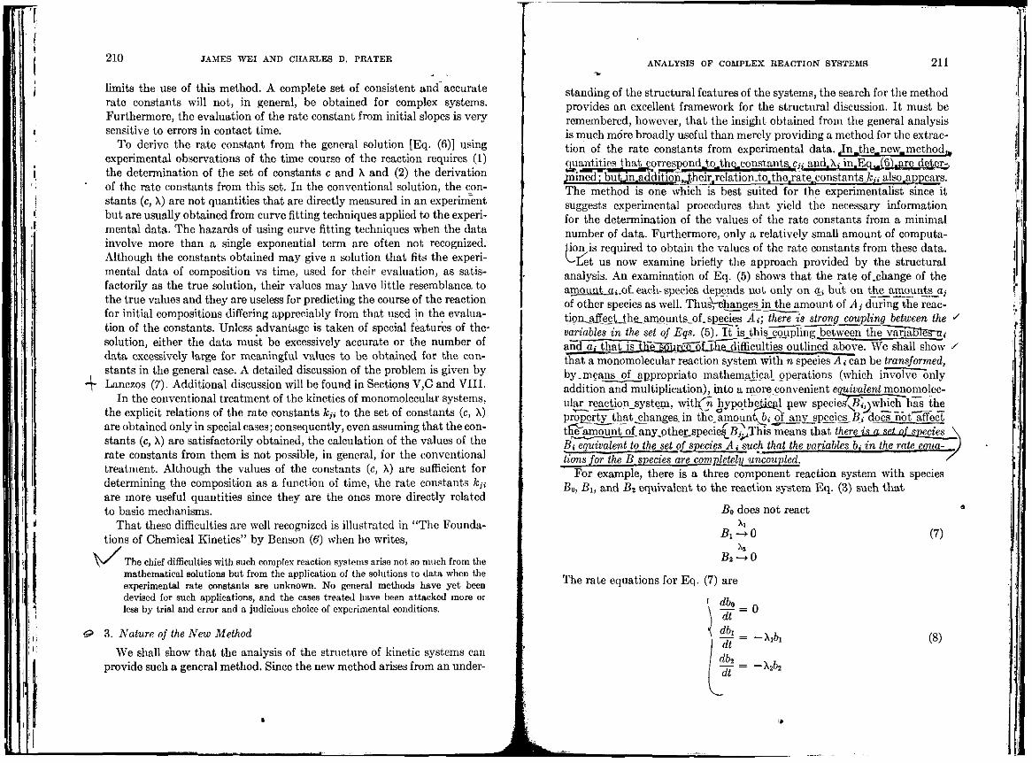
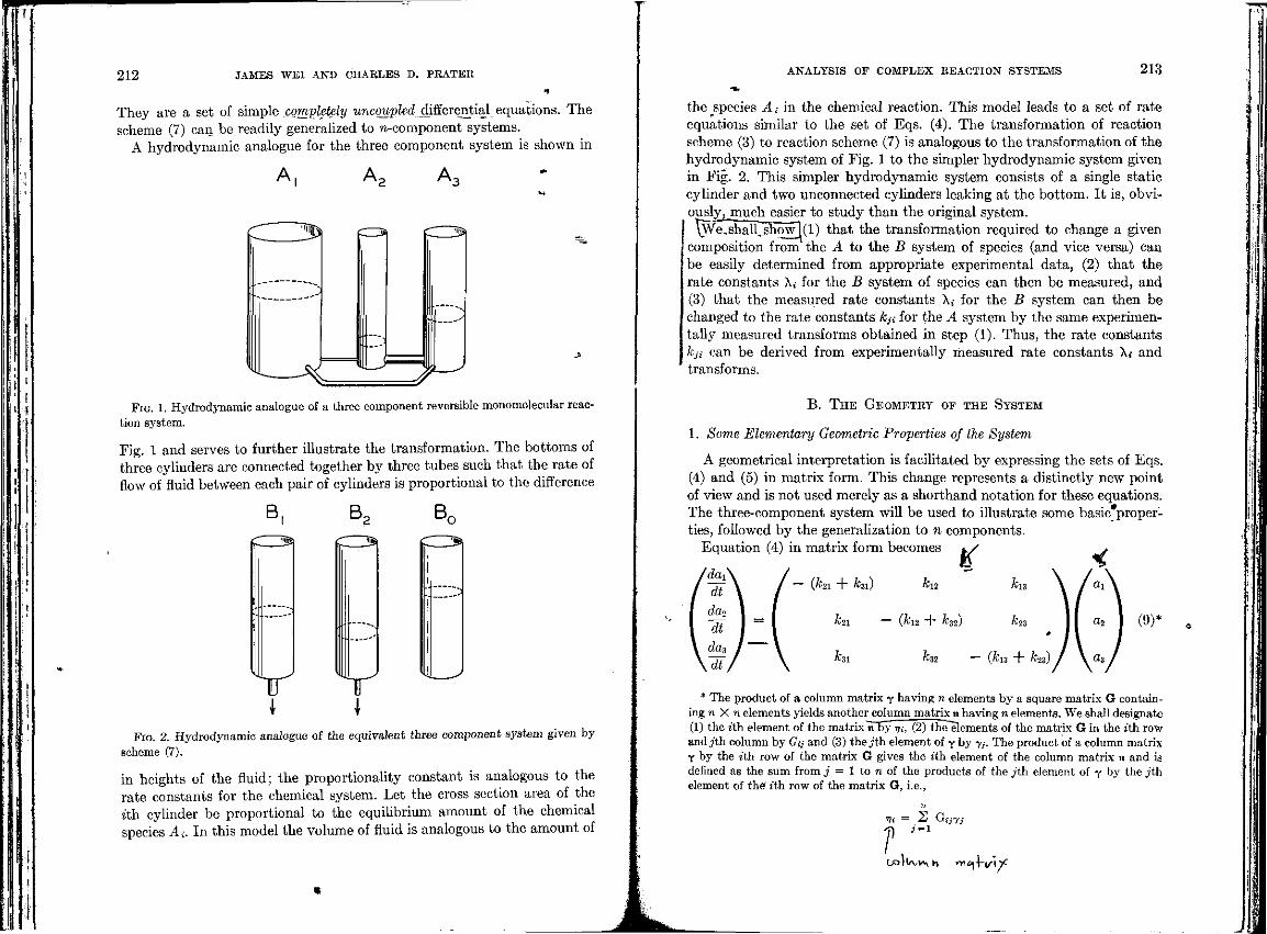
A hydrodynamic analogue for the three component system is shown in
ANALYSIS OF COMPLEX REACTION SYSTEMS 213
FIG. 1. Hydrodynamic analogue of a three component reversible monomolecular reaction system.
Fig. 1 and serves to further illustrate the transformation. The bottoms of three cylinders are connected together by three tubes such that the rate of flow of fluid between each pair of cylinders is proportional to the difference
B, B , B ,
FIG. 2. Hydrodynamic analogue of the equivalent three component system given by scheme (7).
in heights of the fluid; the proportionality constant is analogous to the rate constants for the chemical system. Let the cross section area of the ith cylinder be proportional to the equilibrium amount of the chemical species A». In this model the volume of fluid is analogous to the amount of
the species Ai in the chemical reaction. This model leads to a set of rate equations similar to the set of Eqs. (4). The transformation of reaction scheme (3) to reaction scheme (7) is analogous to the transformation of the hydrodynamic system of Fig. 1 to the simpler hydrodynamic system given in Fig. 2. This simpler hydrodynamic system consists of a single static cylinder and two unconnected cylinders leaking at the bottom. It is, obviously, much easier to study than the original system.
ffl^e.shall,_showl(l) that the transformation required to change a given composition from the A to the B system of species (and vice versa) can be easily determined from appropriate experimental data, (2) that the rate constants X. for the B system of species can then be measured, and (3) that the measured rate constants X. for the B system can then be changed to the rate constants kji for the A system by the same experimentally measured transforms obtained in step (1). Thus, the rate constants kji can be derived from experimentally measured rate constants X,- and transforms.
B . T H E GEOMETRY OF THE SYSTEM
1. Some Elementary Geometric Properties of the System
A geometrical interpretation is facilitated by expressing the sets of Eqs. (4) and (5) in matrix form. This change represents a distinctly new point of view and is not used merely as a shorthand notation for these equations. The three-component system will be used to illustrate some basic*proper-ties, followed by the generalization to n components.
Equation (4) in matrix form becomes iV
(k2i + ksl)
&21 — (&12 + £32)
32 — (&13 + &23)
(9)'
* The product of a column matrix y having n elements by a square matrix G containing n X n elements yields another column matrix n having n elements. We shall designate (1) the z'th element of the matrix n~b'y 17., (2) the~e_ements of the matrix G in the ith row and jth column by <?,*,• and (3) the j'th element of y by y;. The product of a column matrix T by the ith row of the matrix G gives the ith element of the column matrix n and is defined as the sum from j = 1 to n of the products of the jth element of y by the j'th element of the' ith row of the matrix G, i.e.,
Vi — 2s G,-j7j' -n --1
uolivv-th *v\c\\~\/\y:
214' JAMES WEI AND CHARLES D. PRATER
The column matrices
^ and
may be interpreted as vectors in three dimensional space. Let the column matrix c
0
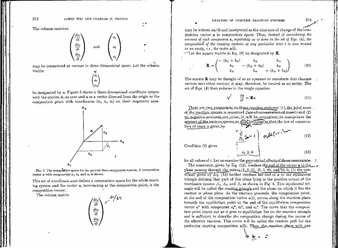
be designated by a. Figure 3 shows a three-dimensional coordinate system with the species A. as axes and a as a vector directed from the origin to the composition point with coordinates (a., a2, a*) on their respective axes.
FIG. 3. The composition space for the general three-component system. A composition vector « with components a_, (__, and a3 is shown.
This set of coordinate axes defines a composition space for the whole reacting system and the vector a, terminating at the composition point, is the composition vector.
The column matrix
ANALYSIS OF COMPLEX REACTION SYSTEMS 215 ^
may be written da/dt and interpreted as the time rate of change of the composition vector a in composition space. Thus, instead of considering the amount of each component ai separately as is done in the set of Eqs. (4), the composition of the reacting systems at any particular time t is now treated as an entity, i.e., the vector a(t).
'-"'"Let the square matrix in Eq. (9) be designated by K.
/— (hi + ksl) ku K = fc_i - (k12 + k32)
\ hi k32 (10)
The matrix K may be thought of as an operator or transform that changes vectors into other vectors; it may, therefore, be treated as an entity. The set of Eqs. (4) then reduces to the single equation
^ £ " « - (ID
There are two constraints-on-these reaction systems: (l)_khe_toJalmass °i____j=Lraa£iJji_i y^^ (2) no____j^ative~amounts._can.arise-_It_.wU^^ the ajnr^nj;^i__Ji_3-_yariou^ law of conservation of mass is given.by
Condition (2) gives
r - j r v
| > - i ) 1 A / * * " "
w -
a > 0
(12)
(13)
for all values of i. Let us examine the geometricaLeffectsjoithese^onstraiats-The constraint, given by Eq. (12), confines the end of the vector a to the_
plane passing through the.poirita^(l>J]..0)J(0> 1, 0), and*(0, 0, 1); the com-sTrairit given b"y~Eq. (13) further c6nfines~ihe end of a to the equilateral triangle defining that part of this plane lying in the positive octant of the coordinate system A\, A2, and A3 as shown in Fig. 4. This equilateral triangle will be called the reaction triangle.and the plane on which it lies the reaction or phase plane. As the reaction proceeds, the composition point, at the end of the composition vector __(.), moves along the reaction plane towards the equilibrium point at the end of the equilibrium composition vector a* with component a.*, a2*, and a3*. The curve that the composition point traces out as it goes to equilibrium lies on the reaction triangle and is sufficient to describe the composition change during the course of the effective reaction. This curve will be called the reaction path for the particular starting composition «(0). Thus, the,reaction, plane with one
V
216 JAMES WEI AND CHARLES D. PRATER
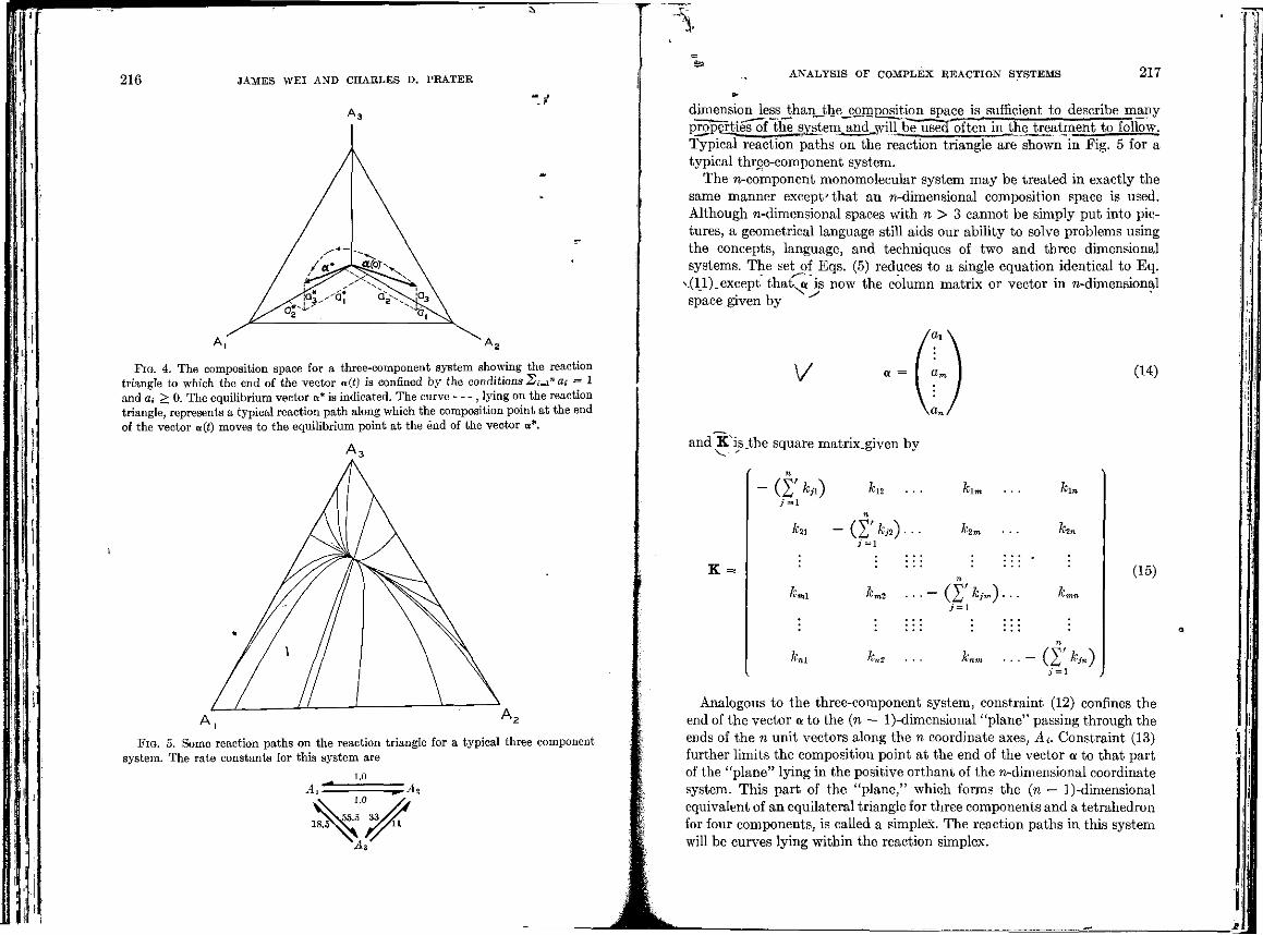
A, m.t
FIG. 4. The composition space for a three-component system showing the reaction triangle to which the end of the vector «(() is confined by the conditions Si_i" a,- = 1 and a. > 0. The equilibrium vector ft* is indicated. The curve , lying on the reaction triangle, represents a typical reaction path along which the composition point at the end of the vector a(_) moves to the equilibrium point at the end of the vector a*.
FIG. 5. Some reaction paths on the reaction triangle for a typical three component system. The rate constants for this system are
1.0 - A, A,:
%
ANALYSIS OF COMPLEX REACTION SYSTEMS 217
dimension less thai^the^omposition space is sufficient to describe many properties of the_sy_stem.andj,vill_be used often in the treatment to follow. Typical reaction paths on the reaction triangle are shown in Fig. 5 for a typical three-component system.
The n-component monomolecular system may be treated in exactly the same manner except'that an n-dimensional composition space is used. Although n-dimensional spaces with n > 3 cannot be simply put into pictures, a geometrical language still aids our ability to solve problems using the concepts, language, and techniques of two and three dimensional systems. The set of Eqs. (5) reduces to a single equation identical to Eq.
\(ll)_except that^ft is now the column matrix or vector in n-dimensional space given by
V a = I a (14)
and K'is.the square matrix.given by
n - ( X ' ^ ' 0 k_2 . . . h,.
n,
hi — ( X ' &&) " " • ^2"
K =
3 =1
km2 . . . — ( J ' kjm)
km
hn
.' = 1
kn2
3=1
(15)
Analogous to the three-component system, constraint (12) confines the end of the vector a to the (n ~ l)-dimensional "plane" passing through the ends of the n unit vectors along the n coordinate axes, A.. Constraint (13) further limits the composition point at the end of the vector a to that part of the "plane" lying in the positive orthant of the n-dimensional coordinate system. This part of the "plane," which forms the (n — 1)-dimensional equivalent of an equilateral triangle for three components and a tetrahedron for four components, is called a simplex. The reaction paths in this system will be curves lying within the reaction simplex.
F
218 JAMES WEI AND CHARLES D. PRATER
\ 2. T/ie Relation of the Rate Constants to Geometric Properties of the System
a. Characteristic directions in composition space. As pointed out in Section II,A thfl^PniircB of the-difficultv with the solution of Eg. (5) is in_the_ strong coupJmg.betweenAhe^yariables a_. I t was also_stated.that.the-diffi-culty can be overcome by transforming compositions in the system of
j ^ p S e l l Z c c u T ^ ^ -spfioifiS whh-rate^quaiio_l£-XQntaming_^ "We shall now show that this equivalent system of hypothetical species exists and demonstrate its properties. To do this we need a geometrical interpretation of the coupling between the variables a*
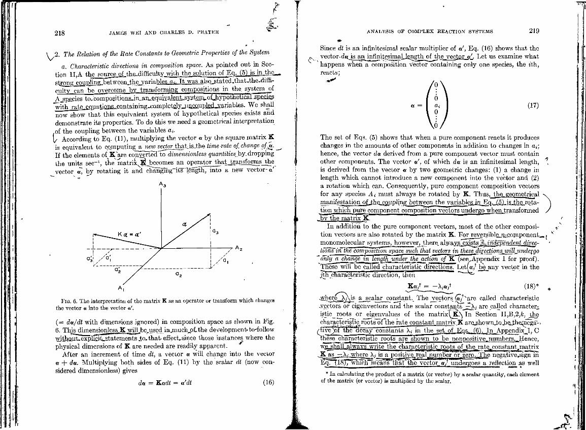
(/ According to Eq. (11), multiplying the vector a by the square matrix K is equivalent to computing a new vector that_is,the time rate of change of^a. ^ If the elements of^Kjire converted to dimensionless quantities \>y. dropping the units sec-1, the'matrix^K. becomes an operator thaj jransformsjhe vector a, by rotating it and ~cliangihg~its~ length, into a new vector- a'
FIG. 6. The interpretation of the matrix K as an operator or transform which change, the vector a into the vector «'.
(= da/dt with dimensions ignored) in composition space as shown in Fig. 6. This dimensionless_K will be.used injnuch^oithe development-to-follow withQut.expljJitu&tatementslo.thateffect.since those instances where the physical dimensions of K are needed are readily apparent.
After an increment of time dt, a vector a will change into the vector a + da. Multiplying both sides of Eq. (11) by the scalar di (now considered dimensionless) gives
da = Kadi = a'dt (16)
ANALYSIS OF COMPLEX REACTION SYSTEMS 219
Since dt is an infinitesimal scalar multiplier of a', Eq. (16) shows that the c^ vector- d«As an jn^ilgsimaljffigth of;the .veclarj/ . Let us examine what
happens when a composition vector containing only one species, the ith, reacts;
(17)
The set of Eqs. (5) shows that when a pure component reacts it produces changes in the amounts of other components in addition to changes in a.; hence, the vector da derived from a pure component vector must contain other components. The vector a', of which da is an infinitesimal length, is derived from the vector a by two geometric changes: (1) a change in length which cannot introduce a new component into the vector and (2) a rotation which can. Consequently, pure component composition vectors for any species A. must always be rotated by K. Thus, the_geometrical manifestation.pfJ^heu£Q.upUng between the variable_jin__Eq. ,(5) is ,the rotation which pure component composition vectors undergo when.transformed
.bv the, matrix K. In addition to the pure component vectors, most of the other composi
tion vectors are also rotated by the matrix K. For reversiblej^cojnponent. monomolecular systems, _hqwever, _there. always exists fi, independent direc-tions'inlhe composition space such that vectors in thesedixedionsjmttjundexgo
"only a change_tn lengthjander_the action of K (see Appendix I for proof). These will be called characteristic directions. Let fa/ be any vector in the Jth characteristic direction, then "* ^
K « / = — Xyft/ (18);
.whereXAis a_i scalar constant._ The vectors., (a/^are called characteristic
.vectors or eigenvectors and the scalar constants__j _Xj are called characteristic roots or eigenvalues of the matrix(jt . \ In Section II,B,2,fc, the characteristic roots~of the rate constant matrix_K are^how-_-_to._beJ;he;__eg_r-v - ^-* f- f.^-.-J&!Vlt£. _________________—--^*M™"**^^* " X
^tiye_)of the decay constants Xt- in the set_o.LJ^as^6).^ia^ppendix_i_I. C these characteristic roots are shown to be nonpqsitive_.numbersvHence, we_shalL.alwavs write the charactCT^^
. K a s ^ X i . where X,- i s a positive, real numberjar zero._The negative^signln Eq^l8),''whlch*^rieahs that*the vector, a / undergoes a reflection as well
* In calculating the product of a matrix (or vector) by a scalar quantity, each element of the matrix (or vector) is multiplied by the scalar. ^
* '
220 JAMES WEI AND CHARLES D. PRATER
as a change in length under the action of the matrix K, does not change our arguments.
. Combining Eqs. (11) and (18), we obtain
V ^ - " W * (19)
5 The|tchami_leristic_directions-Ahe Xj. +Vi r_ -f +!-_/__ t»n + n r\¥ />Vi ii T. cm __-F _-.-.' Hn v.rt-m'i c? rtTi lir ITH **_ .' " \\~ in _-_#-_»-_-» *-\li-that, the rate_ofchange^^t^gpends only on aj Tit.is completelyjincoupicd
.from.yectors along other chVfacteristicdirections_,Tbe characteristic directions can be interpreted as representing pure components in the following manner. Any set of n independent coordinate axes may be used to provide the components for the representation of a vector as a column matrix. Therefore, the n independent characteristic directions can equally well serve as coordinate axes for composition space instead of the first choice. This first choice was made by interpreting the set of pure components Ai to be the coordinate axes; this choice will be designated the natural or A system of coordinates. We-ghalLchoose^the—n,characteristic_diracJions.,a.s
^a n e ^ s e ^ ofj^oordin^ choice-interpret them..as arset.of Jivpoth&ticaLjieiv^pecies^-^, We shall designate
This tire characteristic or B system of coordinates. We may also consider Bj as a special package of A. molecules because in the reaction they transfer as a unit.
Let some particular vector in each of the jth characteristic directions be chosen as a unit vector for this direction. The amount of each of the new characteristic species Bj, e^p resged.as.multiples, of. the..unitTvector.in.the ith direction, wiU.be'o!esignatedl3y_i-)j---and.thacomposition vectors expressed as a columa^Tj_itrix--in-the-J^coordina-te^systemj3y. g,.i.e., for an ^-component system § is the column matrix
by 5 =
b«-i.
(20)
The round brackets of Eq. (14) and the square brackets of Eq. (20) are used to distinguish between column matrices written in the A and B systems respectively.
It must always be remembered that we.are-interpreting a and.,B_as dif-feren_a-epresei].tations.of.th&dSame vector obtained by. changing-tha coordinate axes while the vector remains fixed j n sP^£g^l^s transformations) ...This is in contrast to an interpretation in which the coordinate axes remain fixed in space but the vector moves (alibi transformations). An example of
O i l
ANALYSIS OF COMPLEX REACTION SYSTEMS 221
theJatter is the interpretation of the action of K on a as a transformation of a into a new vector a ' in_the same coordinate system as shown in Fig. 6.
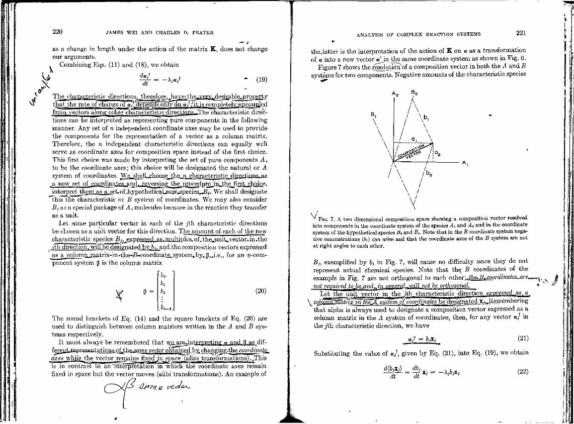
Figure 7 shows the yesolution'of a composition vector in both the A and B systems for two components. Negative amounts of the characteristic species
^ FIG. 7. A two dimensional composition space showing a composition vector resolved into components in the coordinate system of the species Ai and A. and in the coordinate system of the hypothetical species Ba and Bu Note that in the B coordinate system negative concentrations (&_) can arise and that the coordinate axes of the B system are not at right angles to each other.
Bj, exemplified by bx in Fig. 7, will cause no difficulty since they do not represent actual chemical species. Note that the B coordinates of the example in Fig. 7 are not orthogonal to each other•.dhe.BuCoordinatesjxremm
not required to be.am.dAn general^will not be orthogonal. Let the unit vector in the jth characteristic direction e^-pressed^as a
\^ cghmzunainx tn Ihe^AZsyskm^L coordinates be a^ that alpha is always used to designate a composition vector expressed as a column matrix in the A system of coordinates, then, for any vector a, in the j th characteristic direction, we have
tt/ = bjXj (21)
Substituting the value of a / , given by Eq. (21), into Eq. (19), we obtain
d(bjXj) _dbj , (22)
'r
222 JAMES WEI AND CHARLES D. PRATER
since the unitryeptor.Xj is-ennstant. Hence,
^ i i _ L ~ (23)
Thus, the rate, of change of the amount of the pure species Bj is completely independent of other B species. Since each characteristic direction will give a differential equation in the form of Eq. (23), we have
n
>
dbo _ dt
dbi dt
dbm _ dt
dbn-i
— Xo&o
-Xi&i
— Xmfomi
— Xn-i&n-l
(24)
Therefore, the rates of change of the various pure species in the B system are given by the set of simple completely uncoupled differential equations, Eqs. (24), in contrast to the rates of change of the various pure species in the A system, which are given by the set of highly coupled differential equa-
> tions, Eqs. (5). i/ b. The Solution for Monomolecular Reaction Systems in Terms of the
, Characteristic Species. The set of Eqs. (24) may be written in matrix form, analogous to Eq. (11), as
^ - A 3 _ f l - A ?
(25)
where A is thgjate constant matrix for, the, . -ayfltiOTn^f.PPfifi -^-^fl .iY^I^11^ to the rate constant matrix K in the A system. In this case, however, the rate constant matrix is the special n X n diagonal matrix (all diagonal elements are lambda's, all other elements zero)
A = ( - )
Xo 0 . . . 0 0 Xi . . . 0 (26)
,0 0 Xn_i
It is shown in Appendix I that all the characteristic roots are real numbers -<0. Therefore, the solution to the set of Eqs. (24) is
ANALYSIS OF COMPLEX REACTION SYSTEMS 223
(27)
bo = &o°e-^ bs = bi0e-^
™ ^ I'm — um K •**"' :
bn-i = &n°-_e-*-"
^ - ^ J i l ^ H a ^ ^ l u e j ^ i . a t J j m Q , , f i ^ . O J
According to Eq. (27), when Xj > 0 the amount bj. of this species reacts away to zero concentration as t —» » . The law of conservation of mass must hold for the B system and the amounts bj of all the B species cannot be zero simultaneously. I t follows, therefore, that a<t leastjjflj^-QE-the- charao— teristic.roots. say. — Xn. must be zerq_so,lthat..&n_=J>nlat..all.times.^
At equilibrium, (da*/dt) = 0 for all af. Therefore, Ka* = OJ = 0a*; consequently, the_equilibrium vector_fft-is„a_characteristia_.vector*olLthe system and has a characteristic root of zero. We shall limit our attention to reversible systems in which it is possible to go from any species Ai to any other species Aj either directly or through a sequence of other species. Such systems do not contain subsystems that are isolated from each other and each system has, therefore, a_ unique equilibrium p_QJnU For such systems, there can be no other characteristic vectors with X = 0 since the equilibrium vector, which does not decay, already accounts for all the mass in the system. Let this equilibrium.species correspond.to.the species B0; then the_first„equationpf Eqs. (24) is replaced by
^1 = r\ dt
and its solution in Eq. (27) by
(28)
(29)
Hence, for three component reactions, scheme (3) is replaced by the simple equivalent scheme P „ 2-0 8
__*_-» 0
B2 *
(Bo does not react)
All the mass in the system is accounted for_b^^hejequiUbrium-speeies' _30; the other characteristic speciesdoj-bTaccmjnt for any mass and must,
\ The vector O is
T
224 JAMES "WEI AND CHARLES D. PRATER
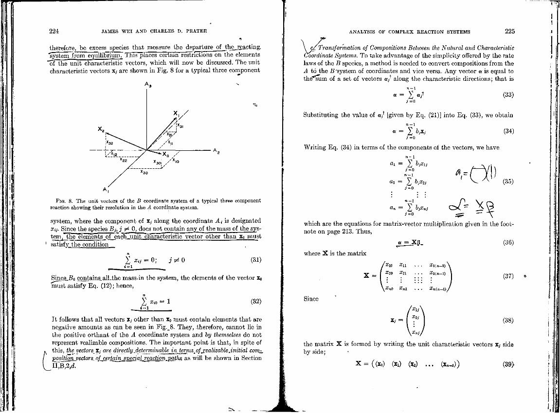
therefore, be excess species that measure the departure of thejgacting, 'system from equilibrium. This places certain restrictions on the elements of the unit characteristic vectors, which will now be discussed. The unit characteristic vectors Xj are shown in Fig. 8 for a typical three component
X,
! X 3 2 ^ ^ ^
L/*« y x22 7
X, / _*>/
jfe? /y / __r * ^ x 0 /
xj /\o _ j /
FIG. 8. The unit vectors of the B coordinate system of a typical three component reaction showing their resolution in the A coordinate system.
system, where the component of Xj along the coordinate Ai is designated Xij. Since the species Bj, j y£ 0, does not contain any of the mass of the system, the elements_qf_each_,unit characteristic vector other than x0 must satisfy the condition
2 z.7 = o; j ^ o (31) *=i
Sinc_e.-Bo contains.alLthe mass-in the system, the elements of the vector x. must satisfy Eq. (12); hence,
X z.o - 1 (32) <=i
It follows that all vectors x;- other than x0 must contain elements that are negative amounts as can be seen in Fig._8. They, therefore, cannot lie in the positive orthant of the A coordinate system and by themselves do not represent realizable compositions. The important point is that, in spite of
Cthis, the vectors Xj are directly determinableJnJermsmojRealizable .initial com-, position vectors.oj certain special reaction.paths, as will be shown in Section I T B A _ T
ANALYSIS OF COMPLEX REACTION SYSTEMS 225
y c/Transformation of Compositions Between the Natural and Characteristic Coordinate Systems. To take advantage of the simplicity offered by the rate laws of the B species, a method is needed to convert compositions from the A to the B 'system of coordinates and vice versa. Any vector a is equal to the sum of a set of vectors « / along the characteristic directions; that is
II~I
« = X « / 3=0
(33)
Substituting the value of a / [given by Eq. (21)] into Eq. (33), we obtain
a = I b,Xj (34) 3=0
Writing Eq. (34) in terms of the components of the vectors, we have n-l
a. = £ bjXij 3=0 n- l
«2 = J bjXtj
A_= (35)
a« = J bp o A \ 3=0
which are the equations for matrix-vector multiplication given in the footnote on page 213. Thus,
«!_L_Xg-
where X is the matrix
X =
Since
Xi =
^l(n-l) %2n—l)
#»(»—_),
(36)
(37)
(38)
the matrix X is formed by writing the unit characteristic vectors Xj side by side;
X = ((x0) (x_) (x2) . . . (Xn_x)) (39)
226 JAMES WEI AND CHARLES D. PRATER
where the round bracket on the sides of each vector is used to emphasize that they are written as a column matrix in the A coordinate system and not as a row matrix. Thus, the matrix X, formed from the unit character-istic vectors x,-, transforms a composition vector written as__> in .theJLsystejn
jnto the_j>ame composition written as_«_in the A system.of. coordinates. The matrix to transform the composition vectors from the A to the B
system is also needed. It is related to the matrix X in the following manner. Let the matrix that transforms a into (5 be designated X - 1 ; then
X-i« = (3 (40)
Substituting the value of a given by Eq. (36) into Eq. (40), we obtain
X- ](X0) = 5 (41)
Equation (41) shows that the matrix X - 1 counteracts the effects of the matrix X on @. It also shows that
X"*X = I (42*)
where I is a matrix whose action on a vector is to leave it unchanged and is, consequently, an identity matrix. For an «-component system, I is the n X n diagonal matrix (diagonal elements unity, others zero)
' l 0 0 0 . . . 0 1 0 0 . . . 0 0 1 0 . . . 0 0 0 1 . . .
,0 0 0 0 . . .
Equation (42) gives the relationship of the matrix X - 1 to the matrix X. For_these particular transformation.matrices,J;here-i&.a^imple method
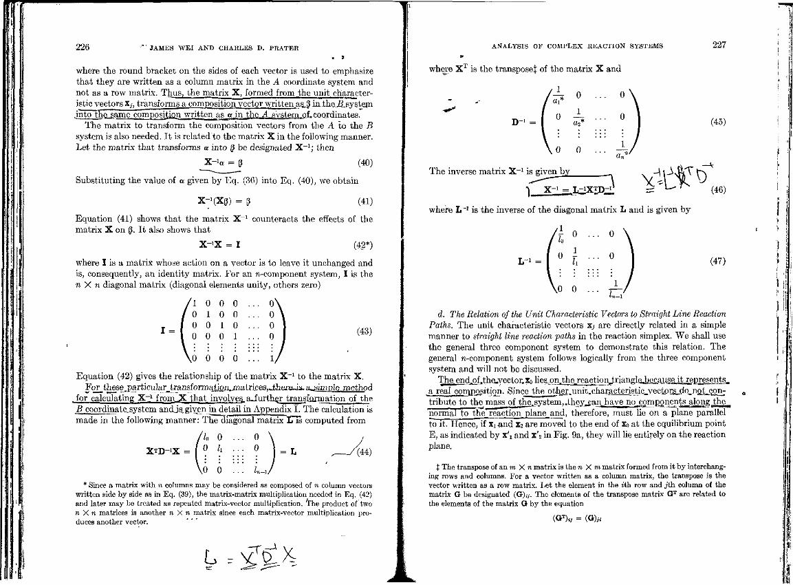
for calculating X"1 from__X that involves, a~furth.gr transformation of the B coordinate.system andjs.given in detail in Appendix I. The calculation is made in the following manner: The diagonal matrix ITis computed from
(43)
X T D ^ X =
0 0
ln-1
= L
* Since a matrix with n columns may be considered as composed of n column vectors written side by side as in Eq. (39), the matrix-matrix multiplication needed in Eq. (42) and later may be treated as repeated matrix-vector multiplication. The product of two n X n matrices is another n X n matrix since each matrix-vector multiplication produces another vector.
L : < g £ . \
ANALYSIS OF COMPLEX REACTION SYSTEMS
where XT is the transpose! of the matrix X and
0
0 - ^ . . . 0
227
^ ' \ 0 a*
1 D"1 = a2* (45)
0 0 . . . ±
The inverse matrix X - 1 is given by . A — - \ y
- ^ A T 0 (« )
where lr1 is the inverse of the diagonal matrix L and is given by
l r* =
V o . . . o to 0 ^ . . . 0
tl
0
(47)
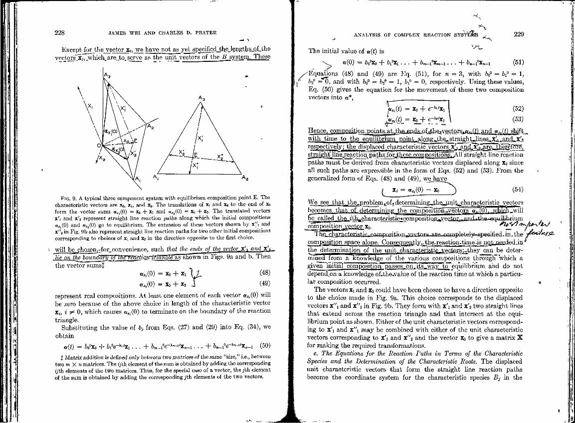
d. The Relation of the Unit Characteristic Vectors to Straight Line Reaction Paths. The unit characteristic vectors Xy are directly related in a simple manner to straight line reaction paths in the reaction simplex. We shall use the general three component system to demonstrate this relation. The general n-component system follows logically from the three component system and will not be discussed.
The,end.of.thft.vector.Xo lies_on.the.reaction^riangIe.because itjgpresents^ . a real composition. Since the otherJunit.characteristic_vcctLoij^do-_not_.CQ,n; tribute to the mass of the.system,.theyj;an_haye•nojcomponentSMaIojig[the normal to l l ie reaction plane,and, therefore, must lie on a plane parallel to it. Hence, if Xi and x2 are moved to the end of x0 at the equilibrium point E, as indicated by x\ and x'2 in Fig. 9a, they will lie entirely on the reaction plane.
t The transpose of an m X n matrix is the n X m matrix formed from it by interchanging rows and columns. For a vector written as a column matrix, the transpose is the vector written as a row matrix. Let the element in the ith row and jth column of the matrix G be designated (G)./. The elements of the transpose matrix GT are related to the elements of the matrix G by the equation
( 0 % = (G),.
J "
! J i
228 JAMES WEI AND CHARLES D. PRATER
Except for the vector x0, we have not as yet specj^dJhe_length§-Qf--the vectors~Xj7^which,are_to.serve as the unit vectors of the j ^ y s t e m . These
FIG. 9. A typical three component system with equilibrium composition point E. The characteristic vectors are Xo, zh and x_. The translations of Xi and x2 to the end of Xo form the vector sums a_,(0) = Xo + x_ and c__2(0) = x„ + x2. The translated vectors x'i and x'_ represent straight line reaction paths along which the initial compositions aXl(0) and «_„(()) go to equilibrium. The extension of these vectors shown by x"i and x"2 in Fig. 9b also represent straight line reaction paths for two other initial compositions corresponding to choices of x_ and x2 in the direction opposite to the first choice.
will be^chosen^for, convenience, such that the ends of the vector__x\ and_XjL^ Jde_onthe boundary of the rm'ctian~tnangle~a,s shown in Figs. 9a and b. Then the vector sumsj
0^(0) = Xo + X! \ ± (48)
«_.(0) = Xo + x2 J (49)
represent real compositions. At least one element of each vector 0.^(0) w m
be zero because of the above choice in length of the characteristic vector x., i 5 0, which causes aXi(Q) to terminate on the boundary of the reaction triangle.
Substituting the value of bj from Eqs. (27) and (29) into Eq. (34), we obtain
a(t) = &o°Xo + bi°e-^Xi...+ ftm-iV^-"**-.. . . + &„-_V-x-"x„~i (50)
J Matrix addition is defined only between two matrices of the same "size," i.e., between two m X n matrices. The zjth element of the sum is obtained by adding the corresponding yth elements of the two matrices. Thus, for the special case of a vector, the jth element of the sum is obtained by adding the corresponding jth elements of the two vectors.
"<„
ANALYSIS OF COMPLEX REACTION SYST "S,
*-_
The initial value of __(.) is v -u
> «(0) *= &0% + &i°x_... 4- fc-iX-i... 4- &n-i°xft-i
229
(51)
^ E q u a t i o n s (48) and (49) are Eq. (51), for n = 3, with _>0° = &i° = 1, •• b2° = 0, and with bQ° = 62° = 1, &i° = 0, respectively. Using these values,
Eq. (50) gives the equation for the movement of these two composition vectors into a*,
1 a_.(0 = Xo 4- e-Xl'x_
il__(ft-= _4-e:"l'X2
(52)
(53)
Hence, composition.points-at_athii£i-ii__j3f_^he^vecto with time to the equilibrium point..along^heustraighUJines^x^i„and,,x'. respectively' the displaced characteristic vectors. x^ Jiad!^3tgI^ii_£gfoTie"J
straightTi^iieaction,pathsiocthese.compositiohs.All straight line reaction paths must be derived from characteristic vectors displaced along Xo since all such paths are expressible in the form of Eqs. (52) and (53). From the generalized form of Eqs. (48) and (49), we have
/ x, = 0^(0) - x0 ) (54)
We see thatJ;he_,problem^of.detennimngJihQ^nit^characteristic vectors becomesMithat of-determining, thet composition-vectoi^_Q:fr(0)."j^ichlwill becajled mtha_ith„characteristit>« compositiojuyecliP, r,,. a n °£l' fl--^iu ilil-ri T' ™ ,
^composHio^vectQr.Xo. ^Uyl^-p^Jt^ Thq"chj\r^tRristiiclC
nTr'pn^t1'nT'ii.VPrt^rt; n y p ^ornplot-alyL-ap-afiifipH in fhp J&attfj^ composition space alone. Consepuenjly^the^agfo the determination of the unit ..characterise e lec tors ;-.thev can be determined from a knowledge of the various compositions through" which a given in-tJaT'comp^sitioir^ and do not depend.on a knowledge of.the-value of the reaction time at which a particular composition occurred. *
The vectors Xi and x2 could have been chosen to have a direction opposite to the choice made in Fig. 9a. This choice corresponds to the displaced vectors x"_ and x"2 in Fig. 9b. They form with __'_ and x'2 two straight lines that extend across the reaction triangle and that intersect at the equilibrium point as shown. Either of the unit characteristic vectors corresponding to x'i and x'\ may be combined with either of the unit characteristic vectors corresponding to x'2 and x"2 and the vector x0 to give a matrix X for making the required transformations.
e. The Equations for the Reaction Paths in Terms of the Characteristic Species and the Determination of the Characteristic Roots. The displaced unit characteristic vectors that form the straight line reaction paths become the coordinate system for the characteristic species Bj in the
230 JAMES WEI AND CHARLES D. PRATER
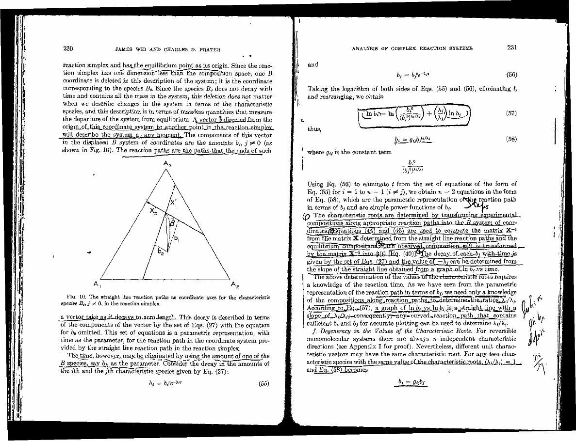
reaction simplex and has_the equilibrium point as its origin. Since the reaction simplex has one dimension" less "tharTthe composition space, one B coordinate is deleted in this description of the system; it is the coordinate corresponding to the species B0. Since the species Bo does not decay with time and contains all the mass in the system, this deletion does not matter when we describe changes in the system in terms of the characteristic species, and this description is in terms of massless quantities that measure the departure of the system from equilibrium. A. vector 3 dire-led irom the origi ri_oLthis__c™rdinat^ will describe the system.at.__anv moment- The components of this vector in the displaced B system of coordinates are the amounts bi j ?* 0 (as shown in Fig. 10). The reaction paths are the paths that.the_ends of such
FIG. 10. The straight line reaction paths as coordinate axes for the characteristic species JSJ-, j _•* 0, in the reaction simplex.
a vector take as __L_f.ecnys tngnrnJength. This decay is described in terms of the components of the vector by the set of Eqs. (27) with the equation for b0 omitted. This set of equations is a parametric representation, with time as the parameter, for the reaction path in the coordinate system provided by the straight line reaction path in the reaction simplex.
The time, however, may. be eliminated by using the amount of one of the ^S^^c jeS j^y_^^£ thepa jamete r . Consider"the decay in*the amounts of the ith and the jth characteristic species given by Eq. (27):
ANALYSIS OF COMPLEX REACTION SYSTEMS
t and
6; = fe/g-*"
231
(56)
Taking the logarithm of both sides of Eqs. (55) and (56). eliminating t, and rearranging, we obtain
thus,
^ ^ j | ^ + f e ) i l ^
bi=.Qijb>^L
(57)
(58)
where p.y is the constant term
.0 (&/) .OU./Ji/
Using Eq. (56) to eliminate t from the set of equations of the form of Eq. (55) for i = 1 to n — 1 (i ^ j), we obtain n — 2 equations in the form of Eq. (58), which are the parametric representation of<*h£ reaction path in terms of bj and are simple power functions of bj. ~-***^5
[Q The characteristic roots are determined by transforming pypfvrimental compositions along appropriate reactionjgaj_ba.J7.tQ t*># Ti system of coor-.dmatt-fljffiquations (4_4) and (46) areused to compute the matrix X ' 1
fronvEKe matrix X deterrnined from the straight line reaction pathsand the is-transformed. equilibriuin^compo^xt^il^Eitch o"5s
by tha-matrbf X ' 1 into ftffi [Eq. (40)].
bi = &.°e->" (55)
he decay._x>f-each-->j with-timc-is given by the set of Eqs. (27) and thqvalue of _—Xj- can be determined from the slope of the straight line obtained .from a graph .of. In 6.--vs time. """*The above determination of tiie values of tin. ditwawteriistiTrroots requires a knowledge of the reaction time. As we have seen from the parametric representation of the reaction path in terms of by, we need only a knowledge of the compositions l,along_reactionl[,paths_tO--determine-»thearatiQS1A./Xj. AccordingJ^Qj-Eq.,,^?), a graph o iM^^vs . In &,• js. a_straight_,lineB[withjLa slope__pf—X.-AT-f-consequentlyr-any- curved -.reaction, path_.that_.coi_ tains sufficient bi and &,- for accurate plotting can be used to determine A./Xj.
/. Degeneracy in the Values of the Characteristic Roots. For reversible monomolecular systems there are always n independent characteristic directions (see Appendix I for proof). Nevertheless, different unit characteristic vectors may have the same characteristic root. For _«_y-two-ehaE-actgristic species with the sa^m_^^e^lUhe_charant,eri8tic roots, JX-/A.).=__!_ and Eo~£582J2__eoj___es
bi = 9ijbj
i i
P^r.
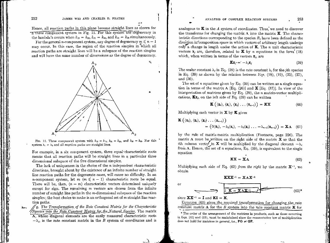
232 JAMES WEI AND CHARLES D. PRATER
Hence, all reaction paths in this plane become straight lines as shown for -aTTl-fee component system in Fig. 11. For this systemT_ie""degeneracy in the lambda's occurs when k12 = k13, kn = hi, and k31 = k32 simultaneously.
For the general n-component system, any degree of degeneracy m ^ n — 1 may occur. In this case, the region of the reaction simplex in which all reaction paths are straight lines will be a subspace of the reaction simplex and will have the same number of dimensions as the degree of degeneracy.
FIG. ] ]. Three component system with fcj_ = fcT., &_i = &_a, and fcji = kz. system Xi = X2 and all reaction paths are straight lines.
For this
For example, in a six component system, three equalr characteristic roots means that all reaction paths will be straight lines in a particular three dimensional subspace of the five dimensional simplex.
The lack of uniqueness in the choice of the n independent characteristic directions, brought about by the existence of an infinite number of straight line reaction paths for the degenerate cases, will cause no difficulty. In an n-component system, let m (m ^ n — 1) characteristic roots be equal. There will be, then, (n — m) characteristic vectors determined uniquely except for sign. The remaining m vectors are chosen from the infinite number of straight line paths in the m-dimensional subspace of the reaction simplex; the best choice to make is an orthogonal set of m straight line reaction paths. tfg. The Transformation of the Rate Constant Matrix for the Characteristic
ySpecies into the Ratejlmsfa The matrix x A, "whose diagonal elements are the easily measured characteristic roots
— Xj, is the rate constant matrix in the B system of coordinates and is
>
\
ANALYSIS OF COMPLEX REACTION SYSTEMS 233
analogous to K in the A system of coordinates. Thus," we need to discover the transforms for changing the matrix A into the matrix K. The characteristic directions corresponding to the species Bj have been defined as the direction in*composition space in which vectors of arbitrary length undergo only a change in length under the action of K. The n unit characteristic vectors Xj are, therefore, related to K by n equations in the form* (18) which, when written in terms of the vectors Xy, are
Kx/-= -XjXj (59)
The scalar constant Ay in Eq. (59) is the rate constant Xj for the j th species in Eq. (30) as shown by the relation between Eqs. (18), (19), (23), (27), and (30).
The set of n equations given by Eq. (59) can be written as a single equation in terms of the matrix A [Eq. (26)] and X [Eq. (37)]. In view of the interpretation of matrices given by Eq. (39), the n matrix-vector multiplications, Kxy, on the left side of Eq. (59) can be written
K((Xo), (Xi), (X_)...(X„_:)) = K X (60)
Multiplying each vector in X by K gives
K((xo), (Xl), (x 2 ) . . . (x„_!) )
= (0(x0), -X1V_E_), -A2(X2) . . . -Xn-i(xn^)) = X A (61)
by the rule of matrix-matrix multiplication (Footnote, page 226). The matrix A must be written on the right side of the matrix X so that the .th column vector in X will be multiplied by the diagonal element — X, from A. Hence, the set of n equations, Eq. (59), is equivalent to the single equation
KX = X A (62)
Multiplying each side of Eq. (62) from the right by the matrix X - 1 , we obtain
KXX- 1 = X A X - '
or
since XX" 1 = I and KI = K. Equation (63) gives the_required Jransformation for changing_the_rate
constant matrix A for the B system into the rate constant matrix K for
* The order of the arrangement of the matrices in products, such as those occurring in Eqs. (62) and (63), must be maintained since the commutative law of multiplication does not hold for matrices in general, i.e., PG ^ GP.
w~*
*
-
_3>
234 JAMES WEI AND CHARLES D. PRATER
tibe_^sy_stem and involves the same transformation matrices X and X - 1
which efTectLtheJc-Janges between'a''ancrgrThus,' the~matrix~K~whdSe'off~ "^diagonal elements are the individual rate constants of Eq. (5), can be calculated from measured characteristic vectors Xy and characteristic roots — Xy.
h. Simplification and Advantages of Introducing Relative Values of the Rate Constants. We have seen t h a i the unit ch-n-pftpristip V^M™* vf a n d the lambda ratios, X,/Xy, can be o'etierminori withniit.an-explicit consideration of theMreac.tion_time—tha,tA&^h£,u^£QMmbewobtaw£dJroniMjiinowledge of ih.p^>na.ri.mi,!L. cnw.pnri.tinnR.JhTmujK. mhirh n.rti^iln.KrinitiafcqmpQ^tions Vas& on their wa.v to eauiMbri^Lwithmt^egaza]jQj,he^lim.e at which the various composition^.occur. We shall show now that the rate constants fcyf_can_bj*, determined to within a constant farctdFXrelative rate constantsJtJ_rom„the fatios~A'7/Xy~and'the vectors"x7"a"nd, consequently, without an explicit ...consideration of reaction time. This is fortunate since the value of the_reaction timej^ujxed_tq_ produce a given" co"mpbsitionjs_u.su^ least repro-
"ducible information obtained about a system. Dividing each element of A [Eq. (26)prjy \m and multiplying the entire
matrix by Xm, we have
A = X„
0
0
0
0
0
0 - x , Xm
0
0
0
0
0
- x 2
Xm
0
0
1 0 - x m + 1 : > .
0 0
0
0 0 Xn-i
(64)
or A = XmA' (65)
where A ' is the matrix on the right of Eq. (64). Substituting Eq. (65) into Eq. (63), we obtain
K = X^XA'X"1 (66)
since Xm is a scalar quantity. The matrix*XA'X_i.is a relative rate constant matrix, which we shall designate
K' = XA'X"1 (67)
hence,
K = AmK' (68)
ANALYSIS OF COMPLEX REACTION SYSTEMS 235
Any_one_of_the nonzero relative dementsJzLaSiiJ£-',msay k'_im± may_be_made equal to unity ..by dividina^ach^£l£iQent of K' bv &'/__ giving; a matrix, wliich wULfae d^ignated J(, and whose elements will be designated.by ky,-. Then, <
\yher_e_,ihe_element«/i^imjs.the_elemen^£_ih elements of K are
K ji XfnKjl \r.. = _lii = KJ» 7,' "- lm Xmklr, kg l"lm
(70)
Thus, the jVth element of K is the ratio of the true rate constants kji/kim
for the reaction system. -— i. Application to Pseudomonomolecular Reaction Systems. I t is because relative rate constant matrices can be determined from composition data alone that much of the developments presented for the monomolecular system can be applied to the pseudomonomolecular system. We defined pseudomonomolecular systems in Section I as systems with rate equations of the form
dai = 4> (0.i«i + 0.2<J2 . . . - Y djiat . . . + einan\ (71)
y__i
where <j> may be a function of time and the amounts of the various species and is the same for each rate equation for a given system. The quantities that are included in <f> have a degree of arbitrariness that allows us to select the pseudo-rate-constants 0yr for the system so that at least one of them has the value of unity. ,
The quantity 4> niay be treated as a function of time, <f>(t), since each variable a* of the system is itself a function of time, a.(t). Therefore,
dai <>(t)dt
v1' da • = foai 4- 9i2a2 . . . - 2, 9iiUi • • • + 6™a» = -fc (72>
where T is a new time scale with the differential element dr = 4>(t)dt. Hence, with the new time scale r, the pseudomonomolecular reaction system behaves like a monomolecular reaction system. We cannot determine this time scale without integrating the set of nonlinear differential equations (71) to obtain the functions %(.). Nevertheless, since one of the pseudo-rate-constants 6ji is known to be unity, we do not need any time information to determine the value of these constants; we need only to determine the relative matrix K with the proper element unity. This can bo done from composition data alone without regard to reaction time as we have seen.
! I,
236 JAMES WEI AND CHARLES D. PRATER
Conversely, the composition sequence for any initial composition may be determined from the relative matrix as for the monomolecular system.
— j. Time Contours in the Reaction Simplex. When the time appears explicitly in the equation for the reaction paths, it is as a parameter (see Section II,B,2,e); hence the explicit inclusion of time in the reaction simplex is also parametric and it may be shown by means of contours of constant time as discussed below. The equations for these contours provide a convenient method for computing the reaction paths and for understanding some of the characteristics of these systems. For a given initial composition a(0), there is a corresponding initial composition 0(0) given by
5(0) = X-»«(0) (73)
and for each composition 0(0, there is a corresponding composition a(t) given by
a(t) = Xff(_) »(74)
The compositions 0(0 are given in terms of the initial composition 0(0), by [Eq. (27) in matrix form]
0(0 = expA. 0(0)
where exp A_ is the diagonal matrix
expA. = 0 0
0 e-x,t
0
0 0
e~x?( . .
0 0 0
(75)
(76)
,0 0 0 e-v-ix.
Combining Eqs. (73), (74), and (75), we obtain
o(0 = X(exp A0X~VO) (77)
Let T'i designate the matrix
T" = XfexpA.OX"1 (78)*
* A monomolecular system may be defined in terms of the matrix T' instead of the matrix K. For infinitesimal St,
a(8t) = T««(0) - X(exp AWjX^afO)
- x [ l + A « + A * | j + . . . lx-MO)
Neglecting higher order terms,
«(__) = [I + K5.]a(0) = «(0) + Ka(0)5.
= «(0)+|«(0)_;
This formulation of these systems is useful in many cases. The matrix T' is a stochastic matrix and the group [T'| is a one parameter linear continuous transformation group.
ANALYSIS OF COMPLEX REACTION SYSTEMS
for some particular time U; then
a(U) = T"t_(0)
237
(79)
Equation (79) shows that T'1 transforms a particular initial composition «(0) into its value a(_i) at time h. If we have a set of initial composition points a(0) that forms a curve in the reaction simplex at t = 0, this transform will change the original curve into a new curve representing the time contour at time ti containing the composition points a(.i). Hence Eq. (79) gives the constant time contour as a function of the initial composition.
When the matrix T'1 is applied to the composition a(._), we have, from Eq. (79),
T*a(.0 = (T")3«(0) = a(2.,) (80)
since
Hence,
(T")a = X(expAtl)X-lX(expAt1)X^ = X(expA(2_,))X-
a((m-r- l)k) = T"a(mti) (81)
where m is a positive integer or zero. Equation (81) may be used to calculate the composition points along a reaction path at successive time intervals At = tv Near equilibrium the matrix T*' may give points with closer spacing than desired; in this case, either the matrix (T(i)2 or (T(l)4 may be computed; these correspond to At = 2ti and to At = 4f1; respectively. In the computation of reaction paths, the relative matrix A ' may be used instead of the matrix A. In this case the time t is not actual reaction time but is merely a "bookkeeping" parameter to enable us to calculate successive compositions along the reaction paths.
The constant time contours for monomolecular systems have the interesting and useful property of preserving straight lines and relative distances. When the time behavior of two different initial compositions are known, the time behavior of any initial composition between the two may be obtained by linear interpolation. We shall discuss this for three component systems; it generalizes readily to n components. Let a set of compositions a(0,r) lie along the straight line in the reaction triangle connecting the ends of the vectors «i(0) and a2(0); a(0,r) is given by the equation
a(0,r) = (1 - r)a_(0) + ra2(0) (82)
where 0 ^ r ^ 1. Multiplying Eq. (82) from the left by the matrix T'', we have
T"«(0, r) = «(<_, r) = (1 - r)T*a_(0) + rT"a2(0) (83)
Only the scalar r is a function of the initial composition; hence, Eq. (83) is the equation for compositions lying on a straight line connecting the
jh
238 JAMES WEI AND CHARLES D. PRATER
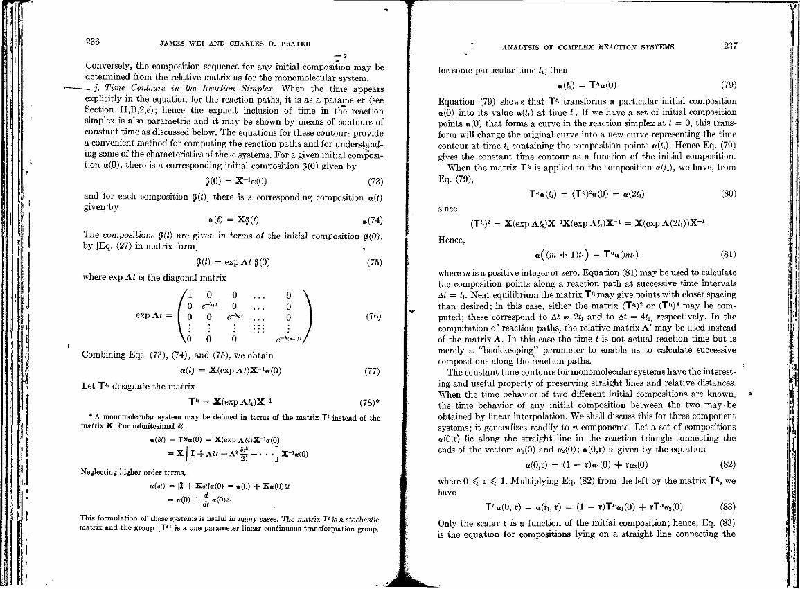
ends of the vectors T'»c_i(0) and T(|a_(0). Therefore, a set of compositions that lie in a straight line at ( = 0 remain on a straight line time contour for all time, and also a set of compositions lying along the sides of the reaction triangle at t = 0 continue to lie along the sides of triangular time contours that shrink in size and change orientation as the reaction proceeds to equilibrium (see Fig. 12). The triangular time contours are, however, not
Fia. 12. Constant time contours for a typical three component system. The initial compositions a(0) lie along the boundary of the reaction simplex.
similar triangles. For n-component systems, the shrinking triangular contours become shrinking simplex contours since Eq. (82) may be generalized to contain n — 1 vectors a.(0) and n — 2 scalar quantities r that depend only on initial composition and not on time. The structure of Eq. (83) shows that the relative distances between composition points are preserved as straight line contours go to equilibrium. The scalar r gives this relative distance, and, since it is not a function of time, a point that is rth of the distance from ai(0) to a2(0) at time . = 0 will also be rth of the distance between T''ai(0) and T''t_2(0) at time h.
k. Comparison Between the New and the Conventional Solutions. The solution obtained using the B system of coordinates must be equivalent to the general solution, Eq. (6), and the transformation from the B to the A system provides the means for showing the equivalence. Substituting Eqs. (27) and (29) into Eq. (35), we obtain
ANALYSIS OF COMPLEX REACTION SYSTEMS 239
a. = Wxio + 6l0^lle-Xl, . . .fcrn-i^Hm-ne-*-" . - - + 0n-ioZicn-i)e-x-,t
a2 = V-C20 + fii^aie"**' . . .fcm_i°:c2(m_i)e-x--,( . . . + fen-i^cr-De"*—'
a-. = b<?xmo 4- 6,°xmle-x". . .bm^xmlm-i)e-^*. . . + 6„_i°a:-,fn-_)e-x"-" (84)
a„ = bQ0x„0 + &i0:c,ie-Xl'.. .bm-iaxn(m-iye-x--'1...+ bn-i^n^e-^-11
A comparison of Eqs. (6) and (84) shows that Xy and cl7 in Eq. (6) are equivalent to Xy and &y°£,-y respectively in Eq. (84). Hence, the general solution Eq. (6) is nothing more than the transformation of 0(0 to the A system of coordinates. Nevertheless, Eq. (84) represents a gain over Eq (6) because its constants have interpretations that give their relation to the rate"constants hi. F_ui-I-£isaQ-^the--into and more_ancurate methods for tho_determinat-on__of_the_constants than the usual curve fitting techniques.
3. The Orthogonality Relations Between The Characteristic Vectors
a. The Origin oi the OrthoaonalituJ?el(itians..ln J^[w(84) ,_the_constants^ fcJi_ar__-Parameter&-detej-rninQd.lfrom the in it Hid_Q___ position and~the constants Xjj and.X,- are the parameters that are determined from experimental j a ta . There are (n2 + n - 1) constants x,y and Xy in Eq. (84). There are, however, only [(n 4- 2)(n — l)]/2 independent constants because additional relationships between the constants xq are-p_j__-_aded-by-4lHnff"l£lw of co-_se-wationj.fjnas_s_-apdJ2lJ;hc^ requires that fc^y* = hiai*.
In Eq. (84^ n characteristic vectors, each' containing n elements, are to be determined. The law of conservation of mass imposes the restrictions of Eqs. (31) or (32) on each vector and, consequently, reduces the number of independent elements of each vector to n — 1. This reduces the number of independent constants in Eq. (84) to n(n - 1) + (n — 1) = (n + \)(n - 1). Consequently, there are (n/2)(n — 1) relations, as yet undetermined, between the constants £,,-; these are provided by the principle of detailed balancing and further reduce the number of independent constants scy.
The principle of detailed balancing provides the means founaking a further transformation to~^tKiTd!j__5ordihate system in wi^^- the charac-teristic directions "are orthogonal to eflch, otrifu__Tfie transformation is discussed in detail in Appendix I, but we have already made use of this orthogonal B system in obtaining the inverse matrix X"1 (Section II,B,2,c). The (n/2)(n — 1) relations provided by the principle of detailed balancing are the requirements that the unit characteristic vectors Xy must be orthogonal to each other after this transformation.
240 JAMES WEI AND CHARLES D. PRATER
The transformation required to changei[ithe-.unit^.characteristic-.vectors X,- into the unit vectors X, for t,he_ orthogonal B system of coordinates is given by. [Eq._(A17)1.Appendix I]
"Sr^"D^X_____^ * (85)
where D *| is the diagonal matrix [Eq. (A10), Appendix I] ' " ' '••••"' w mini II ll—K—p—Mimwt
1
D-H =
'a.'
•-V
0 0 Van*
(86)
To transform the unit vector xy back to the unit vector for the nonortho-gonal B system, we have [Eq. (A18), Appendix I]
|~Xy = D^Xy ) (87)
whereJEq_(AQ),. AppendixJ]
v a?
D^i = 0
0
0
o
(88)
The dot or inner product of two vectors is a scalar quantity and is, in matrix notation,
Xij, X2j • • • Xnj
= XyTX. (89)
where T indicates the transpose of the vector Xy. The inner product between two orthogonal vectors is
l 7*j 3
(90)
There are 2.=iw (n — i) = (n/2)(n — 1) independent orthogonality relations in the form of Eq. (90) for an n-component system; they are the (n/2)(n — 1) additional relations sought.
The orthogonality relation, Eq. (90) may be written in terms of the vectors in the nonorthogonal system;.
^ x/TMx. =_m (91)
ANALYSIS OF COMPLEX REACTION SYSTEMS 241
where D - 1 is the matrix given by Eq. (45). This equation is obtained as follows: Substitution of the value of 5y and X. given by Eq. (85) into Eq. (90) gives
* (B-^Xj)TD-^Xi = 0
Since the transpose of the product of the matrices is equal to the product of the transpose of the individual matrices taken in reverse order, we have
XyTD-^D~^x. = 0
because (D_^)T = D~^ for diagonal matrices. Using D ~ ^ D - ^ = D_1, we obtain Eq. (91).
We shall now show how thesft nrthofronajjty relations ma.vhft.nspd (1) to,porrect-_experimentallv_.measure(JLyectors_Xi_-foii-.lacleoftorthogonality and (2) to ffotRrminft t.hq rfigJQ.ri of the reaction simplex injvhich to_ search for characteristic composition vectors.
b. The Correction of Unit Characteristic Vectors for Lack of Orthogonality. In order to correct a pair of vectors for lack of orthogonality, one of them must be converted to unit length. The square of the length of Xy in the A coordinate system is given by
The required adjustment is _ 1 . * I . LJEV ^
(93)
where Xy is the orthogonal -^characteristic vector of unit length in the A system of coordinates. Let us assume that the vector X* has been determined accurately but errors exist in the vector £,• such that
* . T f 7 = " « « \ " 3 . ' - X i 04)
where the prime on .the subscript.indicates->an-inaccurate-vector.i--The vector y given by
J f - Xy - e,-yX. ^
(95)
by x.T; is orthogonal to x. as shown byrhultiplying"both sides of (84) from the left
X.TY = X**/ - tj&i J (96) = e.y — e.y = 0
sipfe XfTx.- = 1 for vectors oi unit length."Only the vector considered to be accurate in Eq. (95) need bg nf unit. l ^ o l I U i s U g * * * ^ * ^ ^ y'has been purged of the vector Lr_thati,x,;„cQn.tained but | must^aye its.^ length adjusted before ii is either x_. or. X\ ..This procedure may be used to
242 JAMES WEI AND CHARLES D. PRATER
obtain a.self .consistent.set of characteristic vectors..by,correcting_the least accurately determined,, vectors .by...those determined .with-greater accuracy.
c. The Determination of the Region of Composition Space in Which to Search for Characteristic Vectors. After at least one unit characteristic vector, in addition to x0, has been measured, the region of the reaction simplex in which to search for additional characteristic composition vectors may be determined by the use of the transformation to the orthogonal B system of coordinates. Furthermore, the orthogonality relations may be used to reduce by one the number of characteristic vectors that must be measured.
Let us consider the calculation of the value of the last characteristic vector when the other n — 1 vectors, X0, x: . . . xn_2, have been determined experimentally and made self consistent by the above procedure. The last vector, _xn-_i, mus.t_satisfy.the_«._---L relations •
(97)
Xn-s-1*,-! = 0
and_the_requirementsthat-X»_i.is.oLpropex,lcngth. These are sufficient requirements for computing the value of x„_i.
Avector -fi orthogonal to one of the, known vectors, say X0, is written downwIt can be obtained, for example, by making all elements of X0 zero except two, interchanging their position.and placing a negative sign before either one of the two—for instance
is orthogonal to
The vector yi is purged of x\ by applying Eqs. (94) and (95) to give -y-.; repeating the procedure, the vector f2 is purged ot X2 to form y"8 and so on until Y„_I has been calculated.
To calculate x„_x, the vector yn^ is transformed to the nonorthogonal system by applying Eq. (87). Since the vector obtained is not of proper length for its end to lie on the boundary of the reaction simplex when translated by an amount x0, its length is adjusted by scaling the elements of the computed vector. The scaling factor is determined from the requirement that at least one element must be zero and all others equal to or greater than zero when x0 is added to the vector. The vector obtained by
ANALYSIS OF COMPLEX REACTION SYSTEMS 243
this scaling process is xn__. The vector x„__ is converted to a^CO) by adding Xo [Eq. (54)].
The same procedure is used for locating the region of search when fewer than n — y l vectors are known; the process is merely terminated earlier and; the estimate will be less precise.
C. THE STRUCTURE OF REVERSIBLE MONOMOLECULAR SYSTEMS
The above presentation has centered about the development of a general method for determining rate constants from experimental data. During the course of this development, much information has been obtained on the structure of these systems. Some of this information will be briefly summarized and extended in this section.
In the above development the equilibrium point is a structural feature that plays a central role, and it might appear either that its existence has been assumed or that it was implicitly introduced from thermodynamics. This is not the case; it- is a consequence pf jhe following:
/ ( l ) the law of conservation of mass [Eq. (12)], / (2) no negative amounts can arise [Eq. (13)],
[ (3) The-rate of change of each species is a linear function of the V amounts of the various species.
In statement (3), we are not assuming rate Eqs. (5), but only that the rate equations are some linear function of the concentration. These three-statc-u-» ments are also sumcient_to. guarantee that_the. system \vill_conyejge_.tcui single equilibrium poimlj^r_aj^ffident] it is possible, to go from.anvjpecies Af to any other.species.A,either_directly_or. through a sequence of other species.
We have seen that the reaction paths do not spiral about the equilibrium point during this convergence to equilibrium. Neither the above three statements nor thermodynamics is sufficient to guarantee that the reaction does not spiral; it is a consequence of
(4) the principle of detailed balancing. These four statements are also sufficient to guarantee that this kinetic system is consistent with the second law of thermodynamics, i.e., that the Gibbs free energy of the system decreases as the reaction proceeds to equilibrium for isothermal, isobaric systems. Statements^ (l)„through,.(4)i.may be taken as the.axiomaticJormulation.oiLjnQnomoleculaL^yjStejns.and.the---properties that we have discussed in the above sections are consequences of them. Further discussions of the equilibrium point and the convergence to it will be found in Section VII.
We have seen that_all Ti-component reversible,nmonomolecular„systems have n — 1 straight line^eji[liQn-paths^a^nd,J2>^^-l--dRcay..const^.nt^.Ay..
IM
244 JAMES WEI AND CHARLES D. PRATER
The location of the-straip:ht^liriP_rpnrt.;nn_.Dflths..flnfl-J.hft...vg1ii'iACi..rtf the 'gmhda'g d^r^"^ n p n n trhn pxperi^^^t!.l-c^nfinift'><t^i^^^n^^si:;flr-a'"'tom-perature, nature of catalyst, etc. They are..however,.independent.of. the initial composition_us£d--For_a. given_experirnental.xonditionr.the. entire behavior of the reaction system for all initial compositions is specified -when the straight line reaction paths' and th"e~decay constants X'are known. Thus, all quantitative and gualitativeminformation about.the~$ystem..is.contQm&Lin*. the location of the straight line reaction paths and the values, of the lambda's. Furthermore, ail reaction paths, all time courses, and all rate constants are quickly and simply determined from them. In addition, the general-behavior of such systems can be most easily visualized in terms of them; they provide a panoramic view of the entire reaction system and provide the most useful and convenient formulation of the system available.
The excess species Bj, j ?£ 0, provide interesting and „usefulr quantities Jha t measure th"e""cleparture of the system from equilibrium. In addition, the hypothetical B systems of species demonstrate the existence of "transference units," composed of the natural species Ai that change as a unit during the reaction. Additional discussions of the structure of these systems are given in the last two sections.
III. The Determination of the Values of the Rate Constants for Typical Reversible Monomolecular Systems Using
the Characteristic Directions
A. THE TREATMENT OF EXPERIMENTAL DATA
In_the_dis£iissiQnJ^o_follow, we shall consider,the.initial composition for.^, a reaction path as lying on the boundary of the reaction simplexjorjjie following.rea^nsjj.1)" the improved accuracy obtained by using as long a reaction path as possible in the process of locating straight line reaction paths, and (2) the convenience of having at least one A species present in zero concentration in the initial composition. In addition, we shall have occasion to compare the rates of decay of the B species associated with each straight line reaction path and in such a comparison the species Bo, naturally, will not appear (see Section II,B,2,e).
A graphical method may be used to locate the straight line reaction paths in the reaction simplex for a three component system. /\nv cyn,YPnie,nt JM!3L__!__'>Jii ^ its rearilion^path_determine^^ path will bedominated.hythe P sppmps.with the_smallp.st.dpr;ay.r>onst.gnt since, the, other^.species^ill^haye^ decayed TtQ_.a .much .gr.eater._extent.by this-time,, Consequently, a linear extrapolation of the part of-the reaction path near equilibrium back to the side of the reaction triangle gives a new
ANALYSIS OF COMPLEX REACTION SYSTEMS 245
composition containing more of the B species with the smaller decay constant than the original composition and less of the B species with the larger decay constant. This new composition is used as an initial composi-tion.and the process repeated gives a third composition still richer in the slowest decaying >B species. This convergence process is continued until the reaction path obtained becomes a .slraightJine. This straight line reaction path corresponds to the B species with the smallest decay constant. Methods can be given for converging on the straight line reaction path corresponding to the B species with the largest decay constant; it can, however, be calculated from the straight line reaction path corresponding to the slowly decaying B species and the equilibrium composition using the orthogonality relations given in Section II,B,3.
I*L principle, the graphical method used._foLJheJhree^omponent system can_be.uaed.for_a.fo.ur_ component system since its reaction simplex is a tetrahedron; it is not very_cQnvenLent,.hQwever,,to^plot reaction paths in three dimensions and for systems with more components this is not available. Consequently, a method for representing a reaction path is needed that does not involve the reaction simplex directly. In the reaction simplex a reaction path is a single curve in an (n — 1)-dimensional space. A reaction path also can be specified parametrically by n — 1 curves in two dimensional coordinate systems if the amounts of each of the various components ai(i 5* j) is plotted in terms of another one of them, ay, that is monotonic with time. A straight line reaction path in the (n — 1)-dimensional reaction simplex becomes n — 1 straight lines in this two dimensional graph.
The relation of these straight lines to the elements x.y of the unit characteristic vectors are obtained in the following manner. For the n-com-ponent system there are n — 1 equations of the form
(98) /fan® = X 0 - H r ^ x .
representing the n — 1 straight line reaction paths in the reaction simplex. Let us consider the path corresponding to the /th characteristic vector and write Eq. (98) in terms of the components of this vector; this gives
ai = £_o + e~Xltx\i n2 = x20 4- e~*'lx2i : (99) dm = XmQ + (T^Xnl
an =- £„o 4- e-*'lXni
Using Jhe.fact,that-the..equilibrium„.concentratiqn .of. the»mth_-Component o^Mj^_equal -to, _Kmn__and„ using_the_, .ith equation_jiQ_eluninate e~X|t ..from., the other e^ua tioBSy-we obtain .n.~„lequations .of.theform
if'
Ml
246 JAMES WEI AND CHARLES D. PRATER
am = ( a. Xml a. \ , Xml am* — —<ij*) + — °>-
Xji Xji m^j (100)
Thus, a single straight line reactionpath in n — 1 dimensions becomes i -- • ~ mil --;"•' ," . ~ ""• '•'• I |i. i-.iiimiiijuiiwLi....,)ijt
n — 1 straight lines in two dimensions with slopes and mtercepts equal To (xm if Xji) and [am* — ($mi/£ji)a>j*] respectively. ' •*• "Among the B species present in significant amounts in an arbitrary
initial composition of an n-component system there will be, in general, one with a smaller decay constant X than the others. It will be designated the slow B species for this particular initial composition. As for the three component system, the composition along the reaction path near equilibrium contains relatively more of the slow B species and less of the other B species than contained in the initial composition. For an «-component system, the converging procedure applied to the three component system can be used with the two dimensional representation of the reaction path; it gives us the characteristic composition vector corresponding to the slow B species of a particular initial composition.
In order to increase the accuracy, an algebraic least squares fitting of a straight line to the points may be used for calculating the new composition vector rather than the graphical method. The least squares expressions are particularly simple for this case because the straight lines must pass through the equilibrium points, which are considered to be more accurately determined than the composition points along the reaction path. Let (am) and a3) designate the average value of the observed amounts am and ay for those compositions near equihbrium that are to be used to obtain an estimate of a characteristic composition vector. The least squares fitting of a straight line to the points for the two dimensional representation gives n — 1 equations of the form
(am) — am* a,- — ai (aj) - a/ (101)
Before Eq. (101) can be used to determine initial composition vectors, we need to know how to recognize the boundary of the reaction simplex in the two dimensional representation. Use is made of the requirements that am ^ 0 for all values of m and that on the boundary at least one of the amounts am must have the value zero. An examination of the set of Eqs. (101) for each particular case will show which am goes to zero first as ay increases.
There is one additional precaution that must be taken for rz-component systems: after a straight line reaction path has been located, the B species that correspond to it must be removed from other initial compositions that are used to locate new straight line reaction paths. Otherwise, the same straight line path will be obtained all over again if this species happened
ANALYSIS OF COMPLEX REACTION SYSTEMS 247
to be the slow species for this initial composition vector. Any initial composition can be purged of any B species already determined by use of the orthogonal relations (see Section II,B,3).
B . EXAMPLE OF A THREE COMPONENT SYSTEM: BUTENE
ISOMERIZATION OVER PURE ALUMINA CATALYST
1. Experimental Determination of the First and Second Characteristic Vectors
The interconversion of 1-butene, czs-2-butene, and _rcms-2-butene
1-butene hi / /" hi h» \ \ hi
cis-2-butene «-± frans-2-butene hi
(102)
has been studied by Haag and Pines (8) using pure alumina catalyst; they used conventional methods to estimate the values of the rate constants. More recently, Lago and Haag (9) have applied the method presented in this paper to the determination of the rate constants for the same system. We shall use their data obtained at 230° to illustrate the method as applied to three component reversible systems. In this example complete data will be given so that the computations may be reproduced in detail, as a practice example, by those who desire to do so.
Any convenient initial composition such as pure cts-2-butene[is[used to. determine « rpftp-t.inn path t,n the. nR^hhorhood of equilibrium. The approximately straight portion of the reaction path near equilibrium is extrapolated by a straight line back to the side of the reaction triangle, as shown in Fig. 13, to give a new starting composition vector
«(0) =
In the column matrix a, the order of the components are
1-butene as-2-butene
\trans-2-butenej (103)
This composition is used as a new starting composition and its reaction path determined near equilibrium. Since we are very near the straight line reaction path, the twelve composition points given in Table I, forming the approximately straight line portion near equilibrium, is fitted to a straight
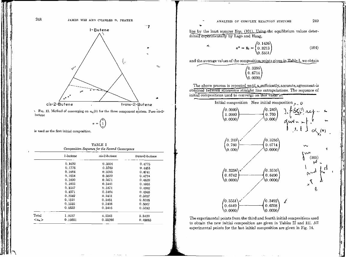
L f
m
248 JAMES WEI AND CHARLES D. PRATER ANALYSIS OF COMPLEX REACTION SYSTEMS 249
cis-2-Butene trans-2-Butene
line by the least squares Eqs. (101), TTsiT1P^-thp equilibrium values deter-mine^experimentally by Lago and Haag,
-4: /0.1436\
a* = xo = I 0.3213 \0.5351/
(104)
\ FIG. 13. Method of converging on ai,(0) for the three component system. Pure cis-2:
butene
- 0 is used as the first initial composition.
TABLE I Composition Sequence for the Second Convergence
and the average values of the composition points givenJnJIahle I, we obtain
/0.3286\ I 0.6714 I Vo.oooo/
The above process is repeated untilj^ufEciently.accurate.agreement-is obtained petween successive straight line extrapolations. The sequence of initial compositions used to converge on this~valOe~is:""" •-•••'»• •»—
Initial composition New initial composition A _ Q
/0.0000\ A).240\ [ 1.0000 ) > 0.760 I
1-butene c_s-2-butene irans-2-butene
0.1622 0.1776 0.1664 0.1654 0.1690 0.1603 0.1537 0.1571 0.1542 0.1521 0.1525 0.1532
0.3604 0.3769 0.3595 0.3622 0.3671 0.3441 0.3471 0.3464 0.3431 0.3451 0.3408 0.3416
0.4775 0.4455 0.4741 0.4724 0.4639 0.4955 0.4992 0.4965 0.5027 0.5028 0.5067 0.5052
Total <am>
1.9237 0.16031
4.2343 0.35286
5.8420 0.48683
vO.OOOO,
' 0 . 2 4 0 y ' 0.760 —
VO.OOO/
' 0 . 3 2 5 8 V 0.6742 J—
^0.0000/
/
/
/ /
/
' 0 .355r 0.6449
V0.0000,
03.000,
'0.3286\ 0.6714]
VO.OOOO/
'0.3510\ 0.6490]
VO.OOOO/
'0.3492\ / 0.6508]
VO.OOOO/
The experimental points from the third and fourth initial compositions used to obtain the new initial composition are given in Tables II and III. All experimental points for the last initial composition are given in Fig. 14.
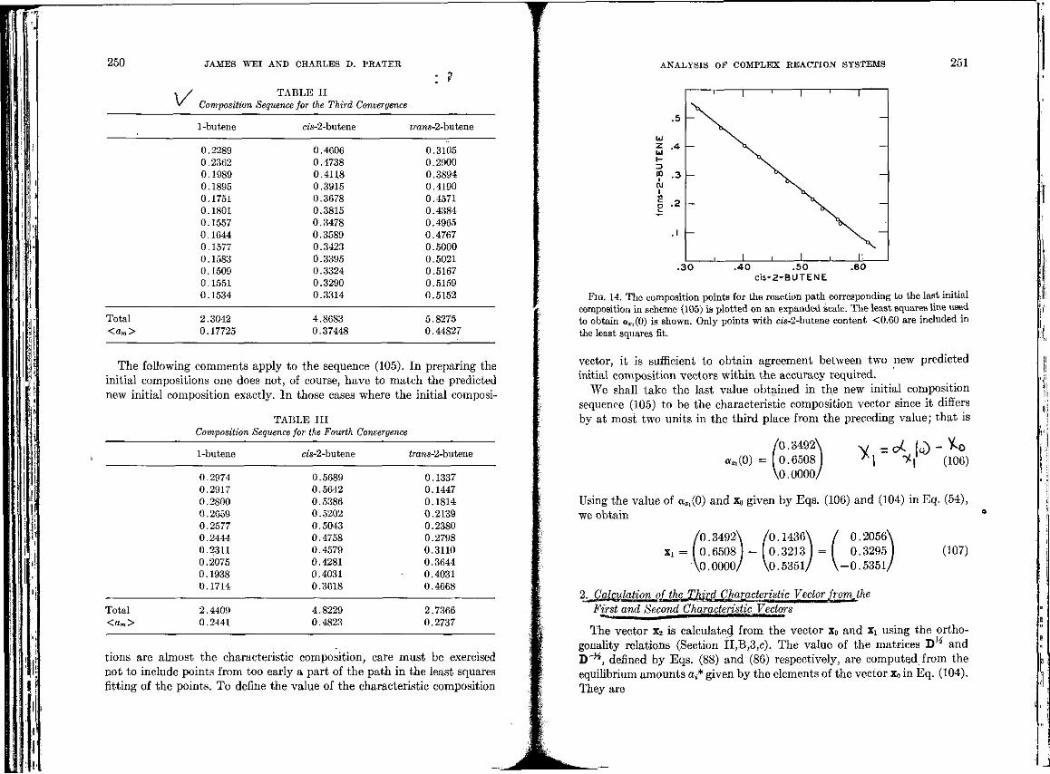
^ r
250 JAMES WEI AND CHARLES D. PRATER
TABLE II Composition Sequence for the Third Convergence
Total <am>
1-butene
0.2289 0.2362 0.1989 0.1895 0.1751 0.1801 0.1557 0.1644 0.1577 0.1583 0.1509 0.1551 0.1534
2.3042 0.17725
czs-2-butene
0.4606 0.4738 0.411.8 0.3915 0.3678 0.3815 0.3478 0.3589 0.3423 0.3395 0.3324 0.3290 0.3314
4.8683 0.37448
tmns-2-butene
0.3105 0.2900 0.3894 0.4190 0.4571 0.4384 0.4965 0.4767 0.5000 0.5021 0.5167 0.5159 0.5152
5.8275 0.44827
The following comments apply to the sequence (105). In preparing the initial compositions one does not, of course, have to match the predicted new initial composition exactly. In those cases where the initial composi-
TABLE III Composition Sequence for the Fourth Convergence
Total <a„>
1-butene
0.2974 0.2917 0.2800 0.2659 0.2577 0.2444 0.2311 0.2075 0.1938 0.1714
2.4409 0.2441
cis-2-butene
0.5689 0.5642 0.5386 0.5202 0.5043 0.4758 0.4579 0.4281 0.4031 0.3618
4.8229 0.4823
Jrcms-2-butene
0.1337 0.1447 0.1814 0.2139 0.2380 0.2798 0.3110 0.3644 0.4031 0.4668
2.7366 0.2737
tions are almost the characteristic composition, care must be exercised not to include points from too early a part of the path in the least squares fitting of the points. To define the value of the characteristic composition
ANALYSIS OF COMPLEX REACTION SYSTEMS
T
251
.30 .40 .50 cis-2-BUTENE
.60
FIG. 14. The composition points for the reaction path corresponding to the last initial composition in scheme (105) is plotted on an expanded scale. The least squares line used to obtain ax,(0) is shown. Only points with ci's-2-butene content <0.60 are included in the least squares fit.
vector, it is sufficient to obtain agreement between two new predicted initial composition vectors within the accuracy required.
We shall take the last value obtained in the new initial composition sequence (105) to be the characteristic composition vector since it differs by at most two units in the third place from the preceding value; that is
/0.3492\ a«(0) = 0.6508]
Vo.oooo/ * l **| (106)
Using the value of o».(0) and Xo given by Eqs. (106) and (104) in Eq. (54), we obtain
/0.3492\ /0.1436\ / 0.2056\ Xi = 0.6508 ) - 0.3213 ) = I 0.3295 J
Vo.OOOO/ \0 .535 l / \ - 0 . 5 3 5 1 / (107)
\aA^M^l^^^L^hemTMX^MhaVP'c^^s^c Victor fromjhe First and Second Characteristic Vectors ** II mi ~~——-—••' • WI.-III..I—.IHI.II'-.'
The vector x2 is calculated from the vector x0 and x_ using the orthogonality relations (Section II,B,3,c). The value of the matrices Dw and \yH, defined by Eqs. (88) and (86) respectively, are computed from the equilibrium amounts a,* given by the elements of the vector x0 in Eq. (104). They are
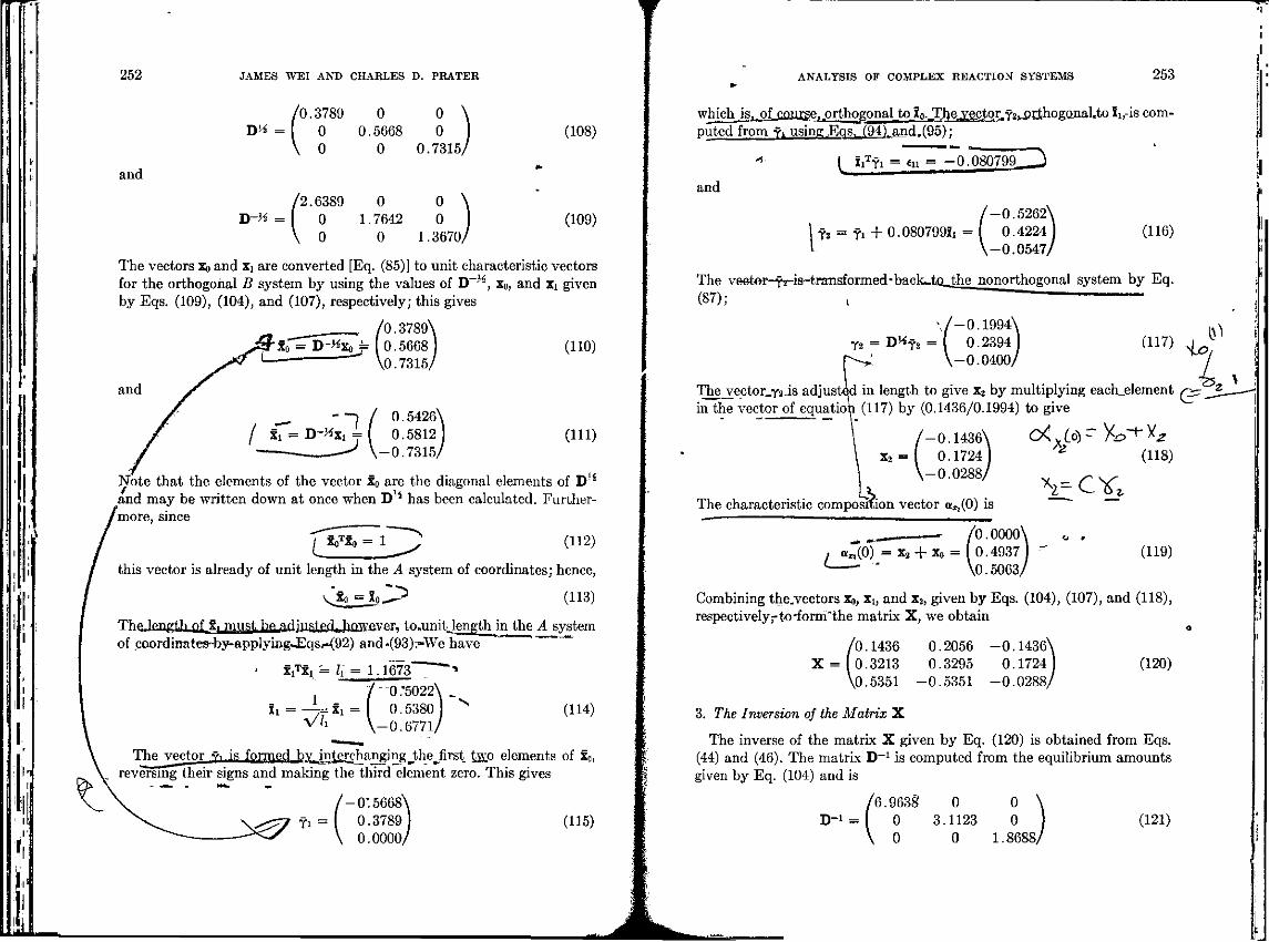
h
252 JAMES WEI AND CHARLES D. PRATER
D^ = 0.3789
0 0
0 0 0.5668 0
0 0.7315
and
D~> = '2.6389 0 0 N
0 1.7642 0 . 0 0 1.3670/
(108)
(109)
The vectors Xo and x_ are converted [Eq. (85)] to unit characteristic vectors for the orthogonal B system by using the values of D - , Xo, and X. given by Eqs. (109), (104), and (107), respectively; this gives
and
/0.3789N
Xo = D-^Xo = 0.5668 \0.7315,
- ~ 7 / 0.5426\ X. = D-*Xi = [ 0.5812]
V —0.7315/
(110)
(111)
Note that the elements of the vector x0 are the diagonal elements of D1J
and may be written down at once when D'4 has been calculated. Further
more, since
I XoTX0 = 1 (112)
this vector is already of unit length in the A system of coordinates; hence,
^ X O _ = 1 Q ^ (113)
Thp lpnfrt.b of x, rniigfr be ndjpg.^JiQwt-vftr, to-unitjength in the A system of coordinateS"by-applying-iEqsJ-(92) and -(93).-We have ' "
x,TXi = k= 1.1673 "*
/ - o : 5 0 2 2 \ _ ll = —=ti = [ 0.5380 S
Vli V-0 .6771/ (114)
The vector vi.is fonned^y^jnterchanging^the first two elements of So, reversing their signs and making the third element zero. This gives
y e ?
/ - 0 . 5 6 6 8 \ T1 = I 0.3789)
\ 0.0000/ (115)
W
ANALYSIS OF COMPLEX REACTION SYSTEMS 253
which igijjjLjaJLU-Cge) .orthogonaljxajio/r^e.^ x_,-is com-puted from YI using Eqs.. (94).. and .(95):
and
1 XiT?i = di = - 0 . 0 8 0 7 9 9 _ 3
/ - 0 . 5 2 6 2 \ I Y- = Yi + 0.080799Ii = ( 0.4224 ) I \ - 0 . 0 5 4 7 /
(116)
The v^6tor-jr^iajtraTisformed'backMtCL-the nonorthogonal system by Eq. (87);
\ / - 0 . 1 9 9 4 \ T2 = D ^ f . = 0.2394 (117)
\ - 0 . 0 4 0 0 /
The vector_Y2-is adjusted in length to give x2 by multiplying each_element in the vector of equation (117) by (0.1436/0.1994) to give
/ - 0 . 1 4 3 6 \ C A ^ - K>"+"Kz x2 = ( 0.1724 * (118)
\ - 0 . 0 2 8 8 / r ^
The characteristic composition vector a2l(0) is "
V
( ? •
^
/o.oooo\ <C(0) = x2 + x 0 = 0.4937
Vo.5063/ (119)
Combining the.vectors Xo, x_, and x2) given by Eqs. (104), (107), and (118), respectively^to-fornTthe matrix X, we obtain
/0.1436 0.2056 -0 .1436 \ X = 10.3213 0.3295 0.1724
\0.5351 -0 .5351 -0 .0288 / (120)
3. The Inversion of the Matrix X
The inverse of the matrix X given by Eq. (120) is obtained from Eqs. (44) and (46). The matrix D - 1 is computed from the equilibrium amounts given by Eq. (104) and is
/6.963§ 0 0 \ D"1 = I 0 3.1123 0 ) (121)
\ 0 0 1.8688/
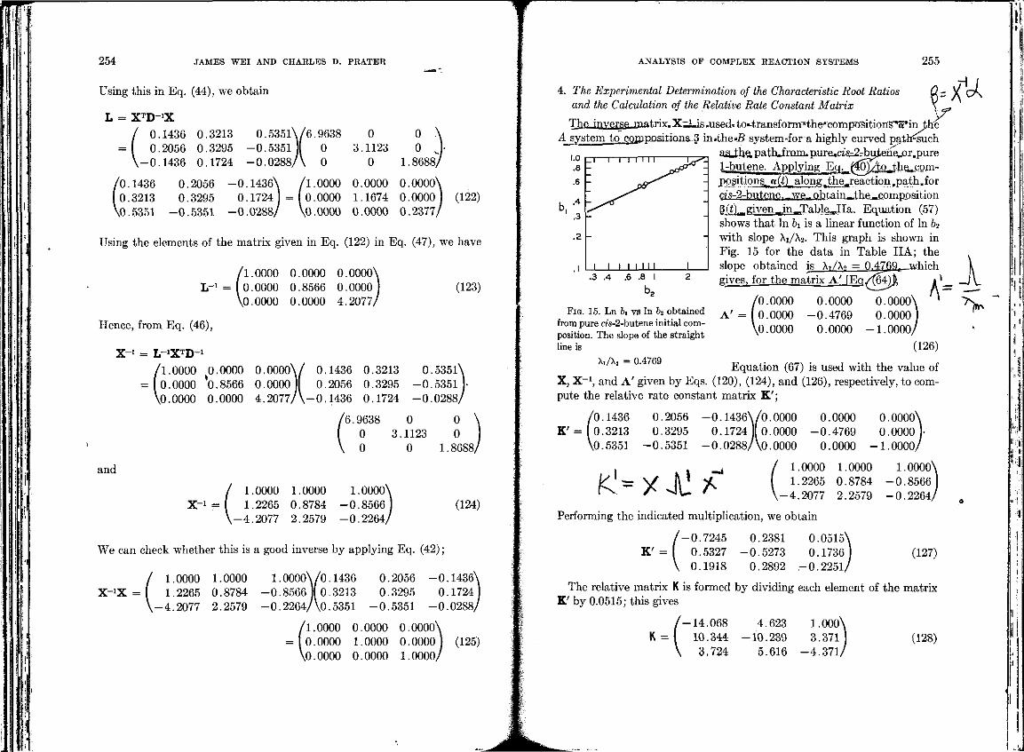
i i
254 JAMES WEI AND CHARLES D. PRATER
Using this in Eq. (44), we obtain
0.535l \ /6 .9638 0 0 -0 .5351 )( 0 3.1123 0 -0 .0288/V 0 0 1.
L = XTD-!X
/ 0.1436 0.3213 = ( 0.2056 0.3295
\ - 0 . 1 4 3 6 0.1724
/0.1436 0.2056 -0 .1436 \ /l.OOOO 0.0000 0.0000\ (0.3213 0.3295 0.1724 = 10.0000 1.1674 O.OOOO] (122) \0.5351 -0 .5351 - 0.0288/ \0.0000 0.0000 0.2377/
Using the elements of the matrix given in Eq. (122) in Eq. (47), we have
/l.OOOO 0.0000 0.0000^ l r 1 = I 0.0000 0.8566 0.0000
VO.0000 0.0000 4.2077, (123)
Hence, from Eq. (46),
X 1 = I r ^ D 1
/l.OOOO = ( 0.0000
Vo.oooo
0.0000 o.ooooV *0.8566 0.0000 0.0000 4.2077/ '
0.1436 0.3213 0.535l\ 0.2056 0.3295 -0 .5351 )•
•0.1436 0.1724 -0 .0288 /
Z6.9638 0 0 I 0 3.1123 0 V 0 0 1.
and
/ 1.0000 1.0000 1.0000\ X"1 = I 1.2265 0.8784 -0.8566
V-4.2077 2.2579 -0.2264/ (124)
We can check whether this is a good inverse by applying Eq. (42);
/ 1.0000 1.0000 1.0000\/0.1436 0.2056 -0 .1436\ X- 'X = ( 1.2265 0.8784 -0 .8566 )( 0.3213 0.3295 0.1724
\ - 4 . 2 0 7 7 2.2579 - 0 . 2 2 6 4 / V 5351 -0 .5351 -0 .0288/
/l.OOOO = 0.0000
Vo.oooo
0.0000 0.0000\ 1.0000 0.0000 J 0.0000 1.0000/
(125)
ANALYSIS OF COMPLEX REACTION SYSTEMS
4. The Experimental Determination of the Characteristic Root Ratios and the Calculation of the Relative Rate Constant Matrix
255
The inverse.matrix.X^Lis.used-to^-transform^the'compo^ition'S'5'in the A system to. compositions-g in«the>»-9 system-fora highly curved path^such
a_sJhe. pathJrojrL pure_,a'&^bujtehej3r,pure 1-butene. AppJ .ymg^q^^^to»the^com-positions[rT«(^)_ialongiitheJreaction.path.for a's-2-but;ene1-->ve^obtainJ-Jthe-composition g(.Q._<given_^n.MTable_Jla. Equation (57) shows that In &_ is a linear function of In b2
with slope AI/A2. This graph is shown in Fig. 15 for the data in Table IIA; the slope obtained is A1A2 = 0.4769, _which gives, for the matrix A / [EqX64)
0.0000\ 0.0000]
-1 .0000 / (126)
/O.OOOO 0.0000 A ' = 10.0000 -0 .4769
Vo.oooo 0.0000
A -FIG. 15. Ln &i vs In b2 obtained
from pure cis-2-butene initial composition. The slope of the straight line is
Equation (67) is used with the value of X, X - 1 , and A ' given by Eqs. (120), (124), and (126), respectively, to compute the relative rate constant matrix K';
/0.1436 0.2056 -0 .1436\ /0 .0000 0.0000 0.0000\ K' = (0.3213 0.3295 0.1724 Mo.OOOO -0 .4769 0.0000 •
Vo.5351 -0 .5351 -0.0288/Vo. 0000 0.0000 -1 .0000 /
r ^ X J t ! *
1.0000 1.0000 1.2265 0.8784
, -4.2077 2.2579
Performing the indicated multiplication, we obtain
/ - 0 . 7 2 4 5 0.2381 0.0515\ K ' = ( 0.5327 -0 .5273 0.1736]
V 0.1918 0.2892 -0 .2251 /
1.0000N
-0 .8566 -0 .2264,
(127)
The relative matrix K is formed by dividing each element of the matrix K ' b y 0.0515; this gives
/ - 1 4 . 0 6 8 4.623 1.000N
K = I 10.344 -10 .239 3.371 V 3,724 5.616 -4 .371 ,
(128)
V
I i '»
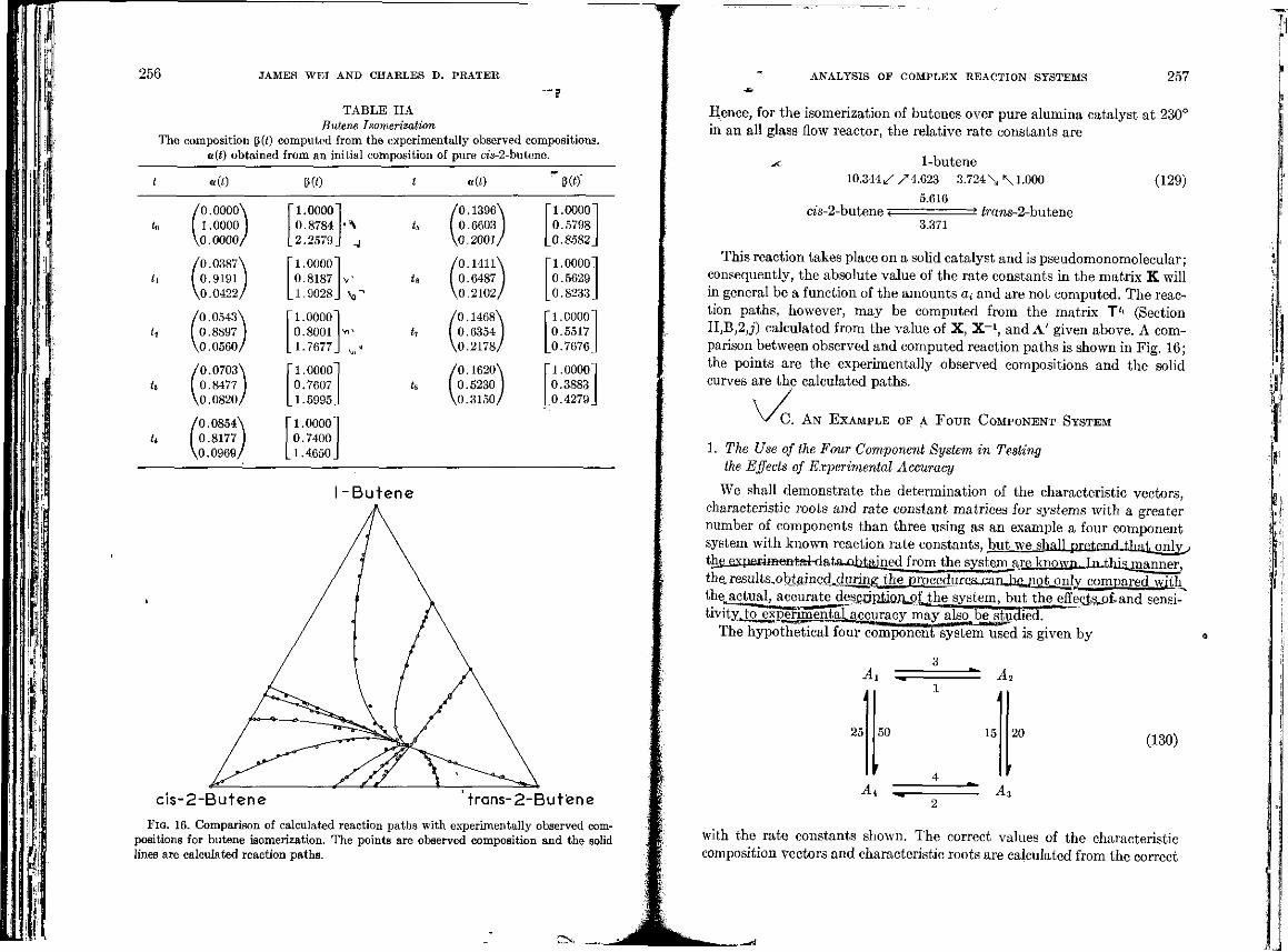
256 JAMES WEI AND CHARLES D. PRATER
TABLE IIA Butene Isomerization
The composition (5(0 computed from the experimentally observed compositions. a(t) obtained from an initial composition of pure cis-2-butene.
t «(0
/0.0000N
1.0000 Vo.oooo,
/0.0387^ 0.9191
V0.0422,
/0.0543N 0.8897
V0.0560y
/0.0703N 0.8477
^0.0820>
'0.0854^ 0.8177
.0.0969^
W) t «(0
1.0000 0.8784 2.2579
A -J
1.0000 0.8187 1.9028_
1.0000' 0.8001 1.7677_
1.0000 0.7607 1.5995J
1.0000" 0.7400 1.4650
V \j
Vi v
'.j
'0.1396^ 0.6603
\0.2001,
^0.1411N
0.6487 V0.2102,
'0.1468^ 0.6354
^0.2178,
''0.1620s
0.5230 .0.3150,
I - B u t e n e
3(0'
1.0000 0.5798 0.8582.
"1.0000' 0.5629 0.8233.
1.0000" 0.5517 0.7676.
1.0000' 0.3883 0.4279
c i s - 2 - B u t e n e trans- 2 - B u t e n e
FIG. 16. Comparison of calculated reaction paths with experimentally observed compositions for butene isomerization. The points are observed composition and the solid lines are calculated reaction paths.
i
ANALYSIS OF COMPLEX REACTION SYSTEMS 257
Hence, for the isomerization of butenes over pure alumina catalyst at 230c
in an all glass flow reactor, the relative rate constants are
1-butene 10.344./ /• 4.623 3.724 \ \ 1.000
5.616 CT's-2-butene < ~* frcms-2-butene
3.371
(129)
This reaction takes place on a solid catalyst and is pseudomonomolecular; consequently, the absolute value of the rate constants in the matrix K will in general be a function of the amounts a. and are not computed. The reaction paths, however, may be computed from the matrix T'1 (Section II,B,2j) calculated from the value of X, X - 1 , and A' given above. A comparison between observed and computed reaction paths is shown in Fig. 16; the points are the experimentally observed compositions and the solid curves are the calculated paths.
C. AN EXAMPLE OF A POUR COMPONENT SYSTEM
1. The Use of the Four Component System in Testing the Effects of Experimental Accuracy
We shall demonstrate the determination of the characteristic vectors, characteristic roots and rate constant matrices for systems with a greater number of components than three using as an example a four component system with known reaction rate constants, but_we_shal1 prpt.pnH tHt^onlyj thg_ejq__^_^nt^<.ataj3l_^^ from thesystemarg_known^In-thi_jmanner, tha results.obtamed.during the proccduresxanJjjLjiQt_only compared with the^ctual, accurate des^dpiJOJipLtheL system, but the_effecJ;sJ1of- and sensi" tivityjUpj^gerime^ may aiso_be_studied.
The hypothetical four^mpon'entVsystem used is given by
25 50 15 20 (130)
with the rate constants shown. The correct values of the characteristic composition vectors and characteristic roots are calculated from the correct
CN,
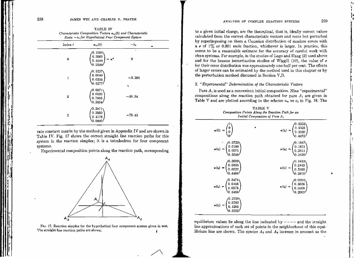
258 JAMES WEI AND CHARLES D. PRATER
TABLE IV Characteristic Composition Vectors aXi(0) and Characteristic
Roots —\ifor Hypothetical Four Component System
T
Index i «..(0) -Xi
I !
/O.lOOOv 0.3000 \ 0.4000 1
V0.200o/
/0.3227V O.OOOO] 0.0396 I
V0.6377/
/0.087K 0.0000 \ 0.7095 I
V0.2034/
/0.2971V 0.2850 \ 0.4179/
vo.oooo/
-5.209
-36.34
-78.45
rate constant matrix by the method given in Appendix IV and are shown in Table IV. Pig. 17 shows the correct straight line reaction paths for this system in the reaction simplex; it is a tetrahedron for four component systems.
Experimental composition points along the reaction path, corresponding
ANALYSIS OF COMPLEX REACTION SYSTEMS 259
to a given initial charge, are the theoretical, that is, ideally correct values calculated from the correct characteristic vectors and roots but perturbed by superimposing on them a Gaussian distribution of random errors with a a of 1% or 0.001 mole fraction, whichever is larger. In practice, this seems to be a reasonable estimate for the accuracy of careful work with clean systems. For example, in the studies of Lago and Haag (9) used above and for the hexane isomerization studies of Wiggill (10), the value of a for their error distribution was approximately one-half per cent. The effects of larger errors can be estimated by the method used in this chapter or by the perturbation method discussed in Section V,B.
2. "Experimental" Determination of the Characteristic Vectors
Pure -4. is used as a convenient initial composition. Nine "experimental" compositions along the reaction path obtained for pure _4_ are given in Table V and are plotted according to the scheme am vs a,- in Fig. 18. The
TABLE V Composition Points Along the Reaction Path for an
Initial Composition of Pure _4i
«(0)
«(ii) =
«&) =
«(d) -
«(.,) -
/0.6725V 0.0189 0.0071 V0.3016'
(/0.500S'\ 0.0306 0.0222 VO.4464
/0.3471V, 0.0468 0.0578 VO.5486
/0.2759V 0.0782 0.1205
Vo.5253-'
«(*»)
«a.)
«*T) =
«(*•) =
/0.2252V 0.1325 0.1950
Vo.4472/
/0.1S47V, 0.1872 0.2611
V0.3670>
/0.1413V, 0.2415 0.3355
V0.2816/
/0.0994^ 0.3036 0.3968
Hl.2002''
TIG. 17. Reaction simplex for the hypothetical four component system given in text. The straight line reaction paths are shown. j
equilibrium values he along the line indicated by and the straight line approximations of each set of points in the neighborhood of this equilibrium line are shown. The species A2 and -43 increase in amount as the
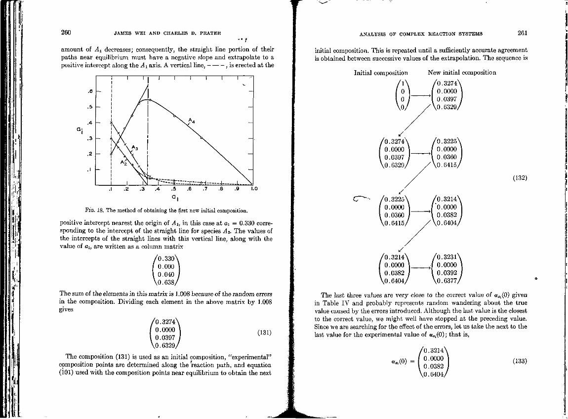
260 JAMES WEI AND CHARLES D. PRATER
amount of Ai decreases; consequently, the straight line portion of their paths near equilibrium must have a negative slope and extrapolate to a positive intercept along the -4_ axis. A vertical line, , is erected at the
ANALYSIS OF COMPLEX REACTION SYSTEMS 261
initial composition. This is repeated until a sufficiently accurate agreement is obtained between successive values of the extrapolation. The sequence is
.6
.b
.4
.3
.2
.1
1 1 1 | 1 1 1 1
x / N.
- r s X i
i i i\| r~—r."::rr_v.-.-$-4-
1 1
-
—-1 L - _ \
Initial composition
.2 .3 .4 .5 a,
.6 .7 .8 .9 1.0
FIG. 18. The method of obtaining the first new initial composition.
positive intercept nearest the origin of Ah in this case at ai = 0.330 corresponding to the intercept of the straight line for species -42. The values of the intercepts of the straight lines with this vertical line, along with the value of a., are written as a column matrix
'0.330v
0.000 0.040
,0.638;
The sum of the elements in this matrix is 1.008 because of the random errors in the composition. Dividing each element in the above matrix by 1.008 gives
CT-
_/ '0.3274' 0.0000 0.0397
,0.6329,
S '0.3225 0.0000 0.0360
,0.6415
vf '0.3214\ 0.0000 V 0.0382 )
,0.6404/
New initial composition
0.3274\ 0.0000 \ 0.0397 j 0.6329/
0.3225 0.0000 0.0360
,0.6415,
'0.3214' '0.0000 0.0382
,0.6404,
'0.3231 0.0000 0.0392
,0.6377,
(132)
'0.3274\ 0.0000 \ 0.0397 I
,0.6329/
(131)
The composition (131) is used as an initial composition, "experimental" composition points are determined along the reaction path, and equation (101) used with the composition points near equilibrium to obtain the next
The last three values are very close to the correct value of aai(0) given in Table IV and probably represents random wandering about the true value caused by the errors introduced. Although the last value is the closest to the correct value, we might well have stopped at the preceding value. Since we are searching for the effect of the errors, let us take the next to the last value for the experimental value of 0^(0); that is,
«*.(0) =
'0.3214' 0.0000 0.0382
,0.6404,
(133)
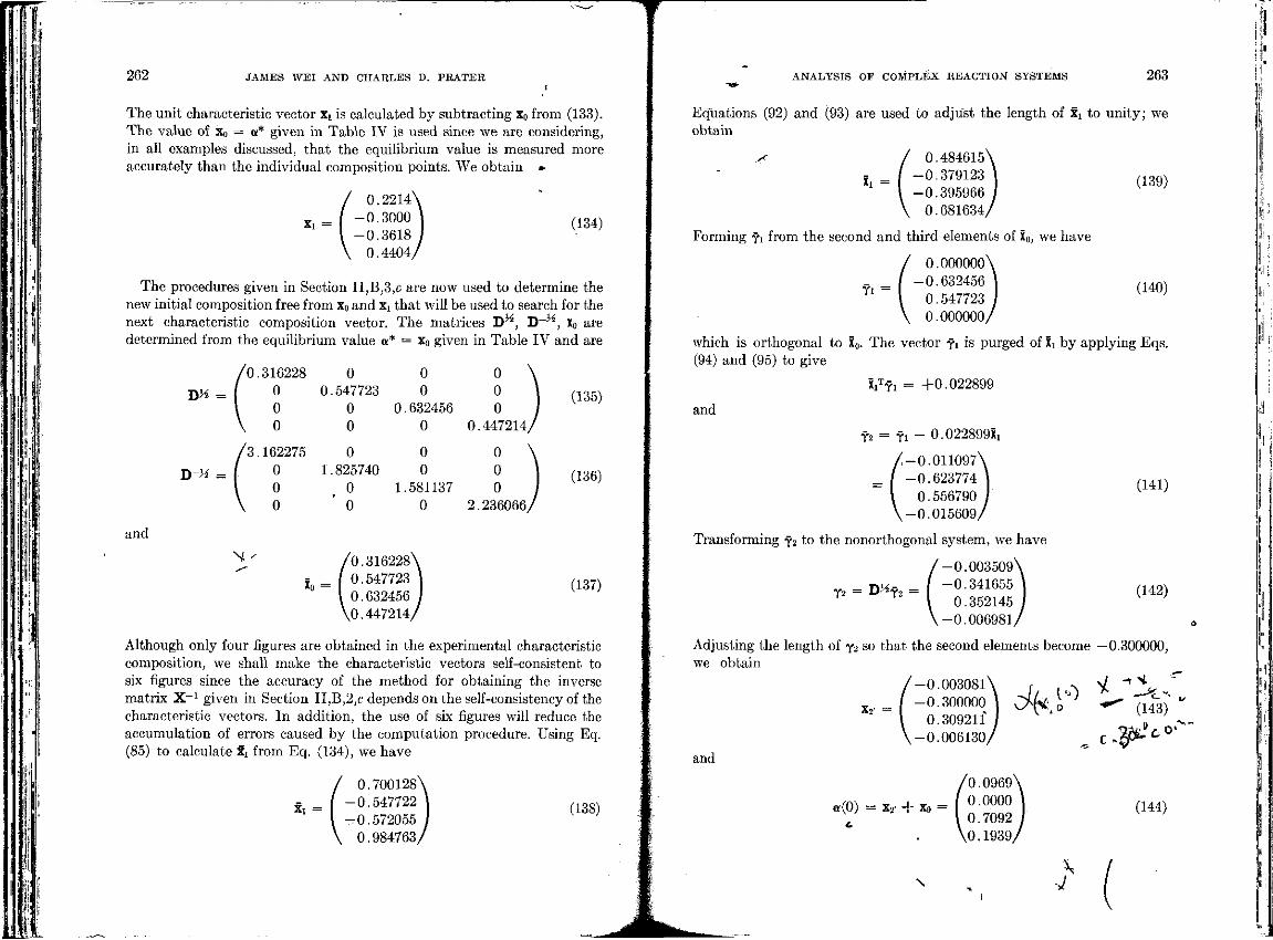
II If
262 JAMES WEI AND CHARLES D. PRATER
The unit characteristic vector Xi is calculated by subtracting Xo from (133). The value of Xo = a* given in Table IV is used since we are considering, in all examples discussed, that the equilibrium value is measured more accurately than the individual composition points. We obtain *
X, =
0.2214 -0 .3000 -0 .3618
0.4404,
(134)
The procedures given in Section II,B,3,c are now used to determine the new initial composition free from x0 and Xi that will be used to search for the next characteristic composition vector. The matrices D^, D - ^ , x0 are determined from the equilibrium value a* = xa given in Table IV and are
D> =
D->- =
0.316228 0 0 0.547723 0 0 0 0
0 0
0.632456 0
0 0 0
0.447214
3.162275 0 0 0 0 1.825740 0 0 0 t 0 1.581137 0 0 0 0 2.236066,
(135)
(136)
and
N '
Xn =
'0.316228 0.547723 0.632456
,0.447214,
(137)
Although only four figures are obtained in the experimental characteristic composition, we shall make the characteristic vectors self-consistent to six figures since the accuracy of the method for obtaining the inverse matrix X - 1 given in Section II,B,2,c depends on the self-consistency of the characteristic vectors. In addition, the use of six figures will reduce the accumulation of errors caused by the computation procedure. Using Eq. (85) to calculate x: from Eq. (134), we have
X. =
0.700128 -0.547722 -0.572055
0.984763,
(138)
ANALYSIS OP COMPLEX REACTION SYSTEMS 263
Equations (92) and (93) are used to adjust the length of Sx to unity; we obtain
x / 0.484615\ X = | -0-379123 \
1 I -0.395966 J \ 0.681634/
Forming ft from the second and third elements of X0, we have
(139)
Ti =
0.000000 -0.632456
0.547723 0.000000,
(140)
which is orthogonal to X0. The vector ft is purged of Xi by applying Eqs. (94) and (95) to give
XiTft = +0.022899
and
y2 = y. - 0.022899X.
( -0 .011097\ -0.623774 \
0.556790 J -0 .015609/
Transforming ft to the nonorthogonal system, we have
(141)
Y2 = D^ft =
-0.003509 -0.341655
0.352145 -0.006981,
(142)
Adjusting the length of y2 so that the second elements become —0.300000, we obtain
-0 .003081\ r -v H ^ -0.300000 \ C % o *
0.309211' / -0 .006130/
x2- = * " (143)
and
'0.0969\
« ( 0 ) = x , - f x 0 = 0.0000 V ! 0.7092 j
,0.1939/
(144)
\ N •J
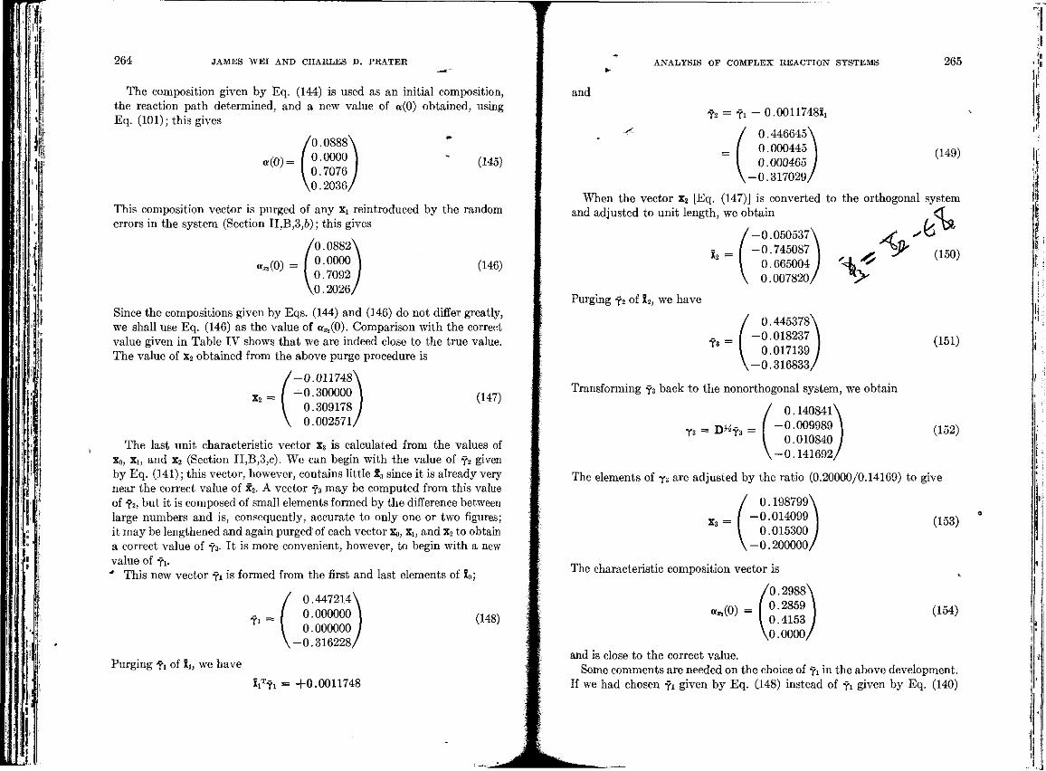
i
I
264 JAMES WEI AND CHARLES D. PRATER
The composition given by Eq. (144) is used as an initial composition, the reaction path determined, and a new value of a(0) obtained, using Eq. (101); this gives
«(0) =
'0.0888 0.0000 0.7076
,0.2036,
(145)
This composition vector is purged of any Xi reintroduced by the random errors in the system (Section II,B,3,&); this gives
«_,(0) =
'0.0882' 0.0000 0.7092
,0.2026,
(146)
Since the compositions given by Eqs. (144) and (146) do not differ greatly, we shall use Eq. (146) as the value of o^fO). Comparison with the correct value given in Table IV shows that we are indeed close to the true value. The value of x2 obtained from the above purge procedure is
x2 =
-0.011748 -0.300000
0.309178 0.00257L
(147)
The last unit characteristic vector x3 is calculated from the values of Xo, Xi, and x2 (Section II,B,3,c). We can begin with the value of ft given by Eq. (141); this vector, however, contains little x3 since it is already very near the correct value of x2. A vector ft may be computed from this value of ft, but it is composed of small elements formed by the difference between large numbers and is, consequently, accurate to only one or two figures; it may be lengthened and again purged of each vector Xo, Xi, and X2 to obtain a correct value of ft. I t is more convenient, however, to begin with a new value of ft. "* This new vector ft is formed from the first and last elements of Xo;
Yi =
0.447214' 0.000000 0.000000
-0.316228,
(148)
Purging ft of X_, we have
jqTTl = +0.0011748
and
ANALYSIS OF COMPLEX REACTION SYSTEMS
y2 = ft - 0.0011748X.
265
*< 0.446645\ 0.000445 \ 0.000465 j
-0 .317029/
(149)
When the vector x2 [Eq. (147)] is converted to the orthogonal system and adjusted to unit length, we obtain tff
-0 .050537\
x2 = -0.745087 ] 0.665004 I ^ 4 ^ 0.007820/ V *
< ty (150)
Purging ft of X2, we have
Ys =
0.445378 -0.018237
0.017139 -0.316833,
(151)
Transforming ft back to the nonorthogonal system, we obtain
Y3 = D^f t =
0.14084l\ •0.009989 j 0.010840 J
-0 .141692/
(152)
The elements of y3 are adjusted by the ratio (0.20000/0.14169) to give
x3
0.198799\ = ( -0.014099 ]
0.015300 I -0 .200000/
(153)
(154)
The characteristic composition vector is
C0.2988\ 0.2859 0.4153 I 0.0000/
and is close to the correct value. Some comments are needed on the choice of ft in the above development.
If we had chosen ft given by Eq. (148) instead of ft given by Eq. (140)
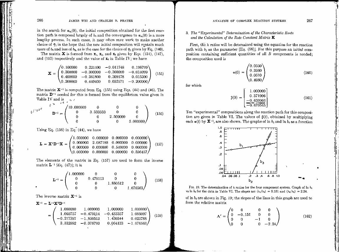
•w
A-"L
til*
266 JAMES WEI AND CHARLES D. PRATER
in the search for als(0), the initial composition obtained for the first reaction path is composed largely of b3 and the convergence to a^(0) is a more lengthy process. In such cases, it may often save work to make another choice of ft in the hope that the new initial composition will contain much more of b2 and less of 63, as is the case for the choice of ft given by Eq. (140).
The matrix X is formed from Xi, x2, and x3 given by Eqs. (134), (147), and (153) respectively and the value of Xo in Table IV; we have
X =
'0.100000 0.300000 0.400000
,0.200000
0.221400 -0.300000 •0.361800 0.440400
-0.011748 •0.300000 0.309178 0.002571
0.198799 -0.014099
0.015300 -0.200000,
(155)
The matrix X - 1 is computed from Eq. (155) using Eqs. (44) and (46). The matrix D^1 needed for this is formed from the equilibrium value given in Table IV and is -v J
D 1 =
10.000000 0 0 0 3.333333 0 0 0 2.500000 0 0 0
0 0 0
5.000000
(156)
Using Eq. (156) in Eq. (44), we have
(1.000000 0.000000 0.000000 o.ooooooX
0.000000 2.087188 0.000000 0.000000 ] , 1 5 7 )
0.000000 0.000000 0.540390 0.000000 I 0.000000 0.000000 0.000000 0.596457/
The elements of the matrix in Eq. (157) are used to form the inverse matrix L 1 |Eq. (47)]; it is
L-1 =
1.000000 0 0 0 0 0.479113 0 0 0 0 1.850512 0 0 0 0 1.676563,
(158)
The inverse matrix X - 1 is
X-1 = L - ^ D - 1
1.000000 1.060757
-0.217397 3.332992
1.000000 -0.4793,14 -1.850513 -0.078793
1.000000 -0.433357 1.430344 0.064133
1.000000 1.055007 0.023788
-1.676563,
(159)
ANALYSIS OF COMPLEX REACTION SYSTEMS 267
3. The "Experimental" Determination of the Characteristic Roots and the Calculation of the Rate Constant Matrix K
First, the X ratios will be determined using the equation for the reaction path with bj as the parameter [Eq. (58)]. For this purpose an initial composition containing sufficient quantities of all B components is needed; the composition used is
«(0) =
for which
5(0) =
'0.0550 0.3960 0.0510
,0.4980,
1.000000 0.371906
•0.659966 " 6 7 9 5 4 5
(160)
(161)
Ten "experimental" compositions along the reaction path for this composition are given in Table VI. The values of §(t), obtained by multiplying each a(t) by X - 1 , are also shown. The graphs of In &i and In b3 as a function
.6 .8 1.0
FIG. 19. The determination of X ratios for the four component system. Graph of In fr. vs hi 6a for the data in Table VI. The slopes are (XiA2) = 0.151 and (X_/A2) = 2.24.
of In b2 are shown in Fig. 19; the slopes of the lines in this graph are used to form the relative matrix
(162)
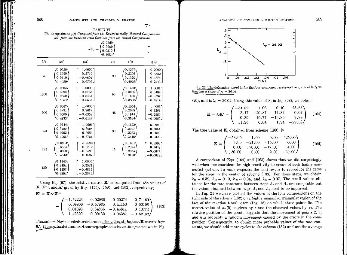
h.;,
i'.lt
¥
268 JAMES WEI AND CHARLES D. PRATER
~i TABLE VI
The Compositions Q(t) Computed from the Experimentally Observed Composition a(t) from the Reaction Path Obtained from the Initial Composition
/0.0550V 0.3960] * 0.0510 I
^0.4980/ a(0) =
l/t «(0 M) l/t «(0 eto
1800
900
450
225
120
/0.0550V, 0.3960 0.0510
Vo.4980y
/0.0603V 0.3893 0.0550 V0.4954
/0.0667v 0.3891 0.0609 Vo.4833/
/0.0744V, 0.3789 0.0702 VO.4766/
/0.0904V 0.3664 0.0888 V0.4543
/0.1140V 0.3454 0.1152 . V0.4254/
1.0000" 0.3719 -0.6601 -0.6795-
1.0000" 0.3763 -0.6431 -0.6567.
1.0000' 0.3678 -0.6359 -0.6147.
1.0001" 0.3698 -0.6056 -0.5764.
0.9999' 0.3612 -0.5599 -0.4837.
1.0000" 0.3543 -0.4891 -0.3531-
90
60
45
30
/15
/0.1257V 0.3396 0.1320 V0.4026''
/0.1453V 0.3060 0.1600
V0.3888/
/0.1554V 0.2938 0.1915
\0.3594/
/0.1622V 0.2697 0.2263" V0.3418''
/0.1601V 0.2394 0.2854
V0.315(V
0.9999 0.3382
-0.4574 -0.2743
1.0001 0.3484
-0.3597 -0.1814.
1.0001" 0.3203
-0.2950 -0.0955.
0.9999" 0.3054
-0.2022 -0.0390-
0.9999" 0.2638
-0.0621 -0.C049.
Using Eq. (67), the relative matrix K' is computed from the values of X, X - 1 , and A ' given by Eqs. (155), (159), and (162), respectively;
K' = XA'X- i
0.02936 -0.57935
0.54866 0.00132
-1 .52223 0.08809 0.01093 1.42320
0.00274 0.41150
-0 .46811 0.05387
0.71160\ 0.00198 \ 0.10774 I
- 0 . 8 2 1 3 2 /
(163)
The^^lue-of-ATis'T[r^gTl-to-deteiTnine_the-value-.of.the_.truevK matrix from K'. I t mayJ-^determined-from-Trgi^h-of-In-62-vs-time,-,as-shown in Fig.
ANALYSIS OF COMPLEX REACTION SYSTEMS 269
.9
.7
.5
.4
.3
.2
1
_ 1
- >i
— N. -
1
1 1 1
* 2 =
1 1 !
1 i
36.02
1 1
--
-
— -
.01 .02 .03 .04 TIME
.05 .06
FIG. 20. The.determination»of-A. for-th&fouE-component system.-The graph of In fc_ vs time has a slope of X2 = 36.02.
(20), and is X2 = 36.02. Using this value of X2 in Eq. (68), we obtain
K = X2K' =
- 5 4 . 8 2 1.06 0.10 3.17 - 2 0 . 8 7 14.82 0.39 19.77 - 1 6 . 8 6
51.26 0.04 1.94
(164)
The true value of K, obtained from scheme (130), is
K =
- 5 3 . 0 0 1.00 0.00 '25.00 3.00 - 2 1 . 0 0 (15.00 0.00 0.00 ,20.00 - 1 7 . 0 0 4.00
50.00 0.00 2.00 -29 .00 ,
(165)
A comparison of Eqs. (164) and' (165) shows that we did surprisingly well when one considers the high sensitivity to errors of such highly connected systems. In some respects, the acid test is to reproduce the zeros for the steps in the center of scheme (130). For these steps, we obtain ktl = 0.39, fcia = 0.10, kA2 = 0.04, and hi = 0.07. The small values obtained for the rate constants between steps A2 and _44 are acceptable but the values obtained between steps Ax and A3 need to be improved.
In Fig. 21 we have plotted the values of the four compositions on the right side of the scheme (132) on a highly magnified triangular region of the face of the reaction tetrahedron (Fig. 15) on which these points lie. The correct value of aXl(0) is given by x and the observed values by 0 . The relative position of the points suggests that the movement of points 2, 3, and 4 is probably a random movement caused by the errors in the composition. Consequently, to obtain more probable values of the rate constants, we should add more cycles to the scheme (132) and use the average
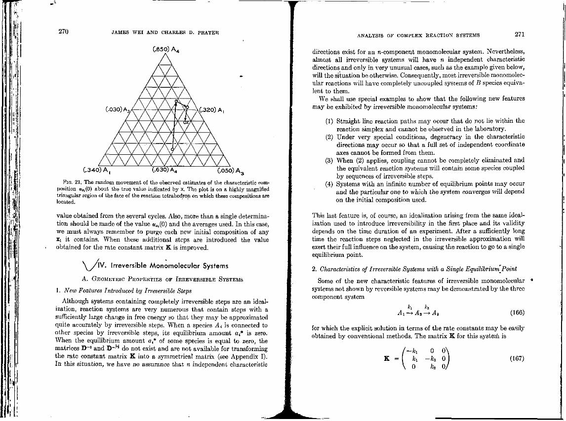
f-fi w
r 'J #1 I f f '
: it l
270 JAMES WEI AND CHARLES D. PRATER
(.650) A 4
(.340) A,
(.030) A (.320) A |
(.630) A (.050) A.
FIG. 21. The random movement of the observed estimates of the characteristic composition asi(0) about the true value indicated by x. The plot is on a highly magnified triangular region of the face of the reaction tetrahedron on which these compositions are located.
value obtained from the several cycles. Also, more than a single determination should be made of the value 0^(0) and the averages used. In this case, we must always remember to purge each new initial composition of any Xi it contains. When these additional steps are introduced the value obtained for the rate constant matrix K is improved.
\ / l V . Irreversible Monomolecular Systems
A. GEOMETRIC PROPERTIES OP IRREVERSIBLE SYSTEMS
1. New Features Introduced by Irreversible Steps
Although systems containing completely irreversible steps are an idealization, reaction systems are very numerous that contain steps with a sufficiently large change in free energy so that they may be approximated quite accurately by irreversible steps. When a species A. is connected to other species by irreversible steps, its equilibrium amount a.* is zero. When the equilibrium amount a.* of some species is equal to zero, the matrices D--1 and D~^ do not exist and are not available for transforming the rate constant matrix K into a symmetrical matrix (see Appendix I). In this situation, we have no assurance that n independent characteristic
ANALYSIS OF COMPLEX REACTION SYSTEMS 271
directions exist for an n-component monomolecular system. Nevertheless, almost all irreversible systems will have n independent characteristic directions and only in very unusual cases, such as the example given below, will the situation be otherwise. Consequently, most irreversible monomolecular reactions will have completely uncoupled systems of B species equivalent to them.
We shall use special examples to show that the following new features may be exhibited by irreversible monomolecular systems:
(1) Straight line reaction paths may occur that do not lie within the reaction simplex and cannot be observed in the laboratory.
(2) Under very special conditions, degeneracy in the characteristic directions may occur so that a full set of independent coordinate axes cannot be formed from them.
(3) When (2) applies, coupling cannot be completely eliminated and the equivalent reaction systems will contain some species coupled by sequences of irreversible steps.
(4) Systems with an infinite number of equilibrium points may occur and the particular one to which the system converges will depend on the initial composition used.
This last feature is, of course, an idealization arising from the same idealization used to introduce irreversibility in the first place and its validity depends on the time duration of an experiment. After a sufficiently long time the reaction steps neglected in the irreversible approximation will exert their full influence on the system, causing the reaction to go to a single equilibrium point.
2. Characteristics of Irreversible Systems with a Single Equilibrium Point
Some of the new characteristic features of irreversible monomolecular systems not shown by reversible systems may be demonstrated by the three component system
h h Ai->A2-+A3 (166)
for which the explicit solution in terms of the rate constants may be easily obtained by conventional methods. The matrix K for this system is
K = '-h o or
h - h o , 0 h 0/
(167)
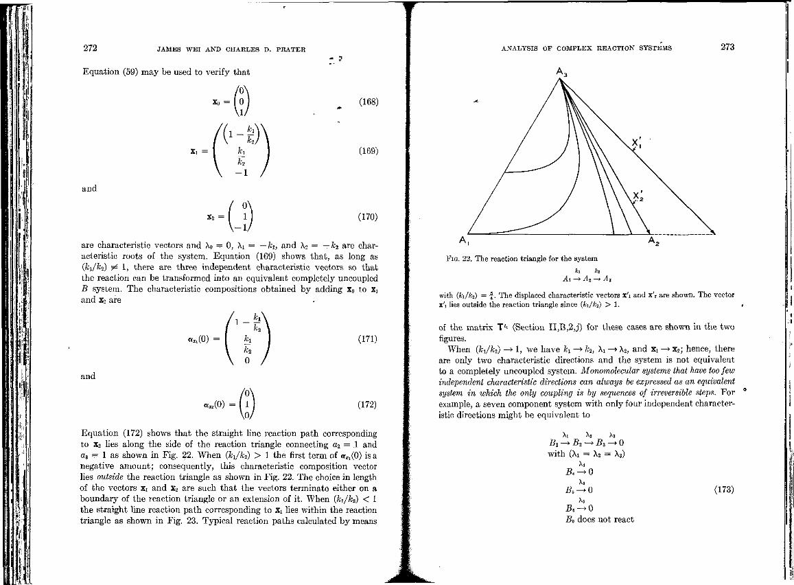
'iff!' w
272 JAMES WEI AND CHARLES D. PRATER - ?
Equation (59) may be used to verify that
X, =
(168)
(169)
and
x2 = (170)
are characteristic vectors and X0 = 0, Xi = — h, and X2 = — h are characteristic roots of the system. Equation (169) shows that, as long as (h/h) ?£ 1, there are three independent characteristic vectors so that the reaction can be transformed into an equivalent completely uncoupled B system. The characteristic compositions obtained by adding x0 to Xi and xs are
a,.(0) = (171)
and
,(0) = (172)
Equation (172) shows that the straight line reaction path corresponding to Xs lies along the side of the reaction triangle connecting a2 = 1 and a3 = 1 as shown in Fig. 22. When (h/h) > 1 the first term of aXl(0) is a negative amount; consequently, this characteristic composition vector lies outside the reaction triangle as shown in Fig. 22. The choice in length of the vectors Xi and x2 are such that the vectors terminate either on a boundary of the reaction triangle or an extension of it. When (h/h) < 1 the straight fine reaction path corresponding to x_ lies within the reaction triangle as shown in Fig. 23. Typical reaction paths calculated by means
ANALYSIS OF COMPLEX REACTION SYSTEMS
A-
273
FIG. 22. The reaction triangle for the system ki i_
Ai -» A2—* A3
with (h/h) = x- The displaced characteristic vectors x'i and x'2 are shown. The vector x'i lies outside the reaction triangle since (h/h) > 1.
of the matrix T'1 (Section II,B,2,j) for these cases are shown in the two figures.
When (h/h) —»1, we have h —> h, Xi —»X2, and Xi —*• X2; hence, there are only two characteristic directions and the system is not equivalent to a completely uncoupled system. Monomolecular systems that have too few independent characteristic directions can always be expressed as an equivalent system in which the only coupling is by sequences of irreversible steps. For example, a seven component system with only four independent characteristic directions might be equivalent to
Ai Xa Aj Bi -> B2 - » B 3 - » 0 with (X. = X2 = X3)
\* B4~*0
Bb^Q (173)
Bt-+Q B0 does not react
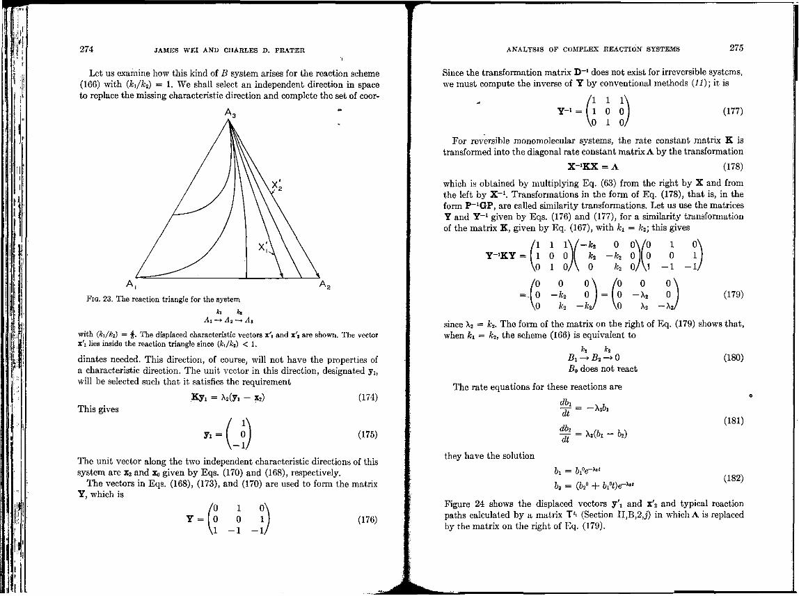
]
274 JAMES WEI AND CHARLES D. PRATER
Let us examine how this kind of B system arises for the reaction scheme (166) with (h/h) = 1. We shall select an independent direction in space to replace the missing characteristic direction and complete the set of coor-
FIG. 23. The reaction triangle for the system *i kt
Ai —> _4_.—» _4.
with (h/h) = 4/. The displaced characteristic vectors x'i and x'j are shown. The vector x'i lies inside the reaction triangle since (h/h) < 1.
dinates needed. This direction, of course, will not have the properties of a characteristic direction. The unit vector in this direction, designated y_, will be selected such that it satisfies the requirement
Ky! = x2(y. - x2) (174) This gives
7. = ( Oj (175)
The unit vector along the two independent characteristic directions of this system are x2 and Xo given by Eqs. (170) and (168), respectively.
The vectors in Eqs. (168), (173), and (170) are used to form the matrix Y, which is
/0 1 0 \ Y = [ 0 0 1 I (176)
ANALYSIS OF COMPLEX REACTION SYSTEMS 275
Since the transformation matrix D_ I does not exist for irreversible systems, we must compute the inverse of Y by conventional methods (11); it is
Y-i ___ (177)
For reversible monomolecular systems, the rate constant matrix K is transformed into the diagonal rate constant matrix A by the transformation
X- 'KX = A (178)
which is obtained by multiplying Eq. (63) from the right by X and from the left by X - 1 . Transformations in the form of Eq. (178), that is, in the form P - 1 GP, are called similarity transformations. Let us use the matrices Y and Y"1 given by Eqs. (176) and (177), for a similarity transformation of the matrix K, given by Eq. (167), with h = h; this gives
(179)
since X2 = h. The form of the matrix on the right of Eq. (179) shows that, when h = h, the scheme (166) is equivalent to
h h BX^>B2->Q
Ba does not react
The rate equations for these reactions are
dhi in.
(180)
(181)
they have the solution
~i =Xa(&i - h)
b2 = (b2° + biH)e-M (182)
Figure 24 shows the displaced vectors y \ and x'2 and typical reaction paths calculated by a matrix T'' (Section II,B,2j) in which A is replaced by the matrix on the right of Eq. (179).
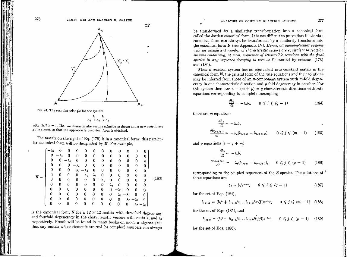
276
-M
_. I;
'I!
JAMES WEI AND CHARLES D. PRATER
A.
x ; = x ;
FIG. 24. The reaction triangle for the system
Ai —» _4. -*_4s
with (h/h) — 1. The two characteristic vectors coincide as shown and a new coordinate y'i is chosen so that the appropriate canonical form is obtained.
The matrix on the right of Eq. (179) is in a canonical form; this particular canonical form will be designated by N. For example,
N =
-Xi 0 0 0 0 0 0 0 0 0 0 0
0 - x a
0 0 0 0 0 0 0 0 0 0
0 0
-Xi 0 0 0 0 0 0 0 0 0
0 0 0
- x 4
x4
0 0 0 0 0 0 0
0 0 0 0
- x 4
x4
0 0 0 0 0 0
0 0 0 0 0
-A* 0 0 0 0 0 0
0 0 0 0 0 0
- x 6
0 0 0 0 0
0 0 0 0 0 0 0
-x f i
0 0 0 0
0 0 0 0 0 0 0 0
-X : X7
0 0
0 0 0 0 0 0 0 0 0
- A T
AT
0
0 0 0 0 0 0 0 0 0 0
-AT
X7-
0 0 0 0 0 0 0 0 0 0 0
-AT,
(183)
is the canonical form N for a 12 X 12 matrix with threefold degeneracy and fourfold degeneracy in the characteristic vectors with roots X4 and A7
respectively. Proofs will be found in many books on modern algebra (12) that any matrix whose elements are real (or complex) numbers can always
ANALYSIS OF COMPLEX REACTION SYSTEMS 277
be transformed by a similarity transformation into a canonical form called the Jordan canonical form. It is not difficult to prove that the Jordan canonical form can always be transformed by a similarity transform into the canonical form N (see Appendix IV). Hence, all monomolecular systems with an insufficient number of characteristic vectors are equivalent to reaction systems containing, at most, sequences of irreversible reactions with the final species in any sequence decaying to zero as illustrated by schemes (173) and (180).
When a reaction system has an equivalent rate constant matrix in the canonical form N, the general form of the rate equations and their solutions may be inferred from those of an n-component system with m-fold degeneracy in one characteristic direction and p-fold degeneracy in another. For this system there are n — (m + p) = q characteristic directions with rate equations corresponding to complete uncoupling
dbi It = ~Xihi 0$i$(q-l) (184)
there are m equations
dt ~ *«*• db
^ ^ = -A3(&Ca+Jo - &(«+,+.>), 0 ^ j ^ (m - 1) (185)
and p equations (s = q 4- m)
dba
dt = — XA
db - ^ — — — X.(6<*+j> — &(H-J+I)), 0$j$(p-l) (186)
corresponding to the coupled sequences of the B species. The solutions of these equations are
^ = bter**, 0$i$(q-l) (187)
for the set of Eqs. (184),
b(q+j) = ( V + &<_+i)°*. • .blg+i)Hi/j\)e-^, 0^j^(m-l) (188)
for the set of Eqs. (185), and
&(B+y) = (&8° + b(.H)H.. .bwW)<r*-', 0$j^(p-l) (189)
for the set of Eqs. (186).
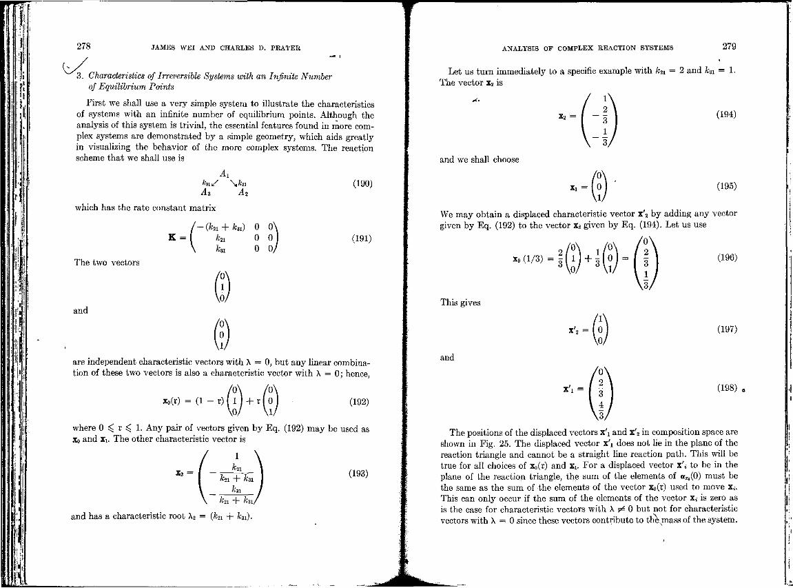
Mi
T
278 JAMES WEI AND CHARLES D. PRATER
3. Characteristics of Irreversible Systems with an Infinite Number of Equilibrium Points
First we shall use a very simple system to illustrate the characteristics of systems with an infinite number of equilibrium points. Although the analysis of this system is trivial, the essential features found in more complex systems are demonstrated by a simple geometry, which aids greatly in visualizing the behavior of the more complex systems. The reaction scheme that we shall use is
Ai hi*f \hi Az A2
which has the rate constant matrix
-(hi + hi) 0 0N
K = I hi 0 0 \ hi 0 0/
(190)
(191)
The two vectors
and
are independent characteristic vectors with A = 0, but any linear combination of these two vectors is also a characteristic vector with X = 0; hence,
Xo(r) = (1 - r ) ( l j + r | o (192)
where 0 ^ r ^ 1. Any pair of vectors given by Eq. (192) may be used as Xo and Xi. The other characteristic vector is
x2 = I -
1 hi
hi ~T" hi hi
(193)
hi + hi,
and has a characteristic root A2 = (hi + &31).
ANALYSIS OF COMPLEX REACTION SYSTEMS 279
Let us turn immediately to a specific example with hi = 2 and £31= 1-The vector x2 is
x2 = - (194)
and we shall choose
(195)
We may obtain a displaced characteristic vector x'2 by adding any vector given by Eq. (192) to the vector x2 given by Eq. (194). Let us use
X„(V3) = | 0 + | ( o ) = ( l (196)
This gives
(197)
and
x'_ = (198)
The positions of the displaced vectors x'i and x'2 in composition space are shown in Fig. 25. The displaced vector x'i does not lie in the plane of the reaction triangle and cannot be a straight line reaction path. This will be true for all choices of x0(r) and x_. For a displaced vector x'i to be in the plane of the reaction triangle, the sum of the elements of as.(0) must be the same as the sum of the elements of the vector x0(r) used to move X*-. This can only occur if the sum of the elements of the vector xt is zero as is the case for characteristic vectors with A ^ 0 but not for characteristic vectors with A = 0 since these vectors contribute to the^nass of the system.
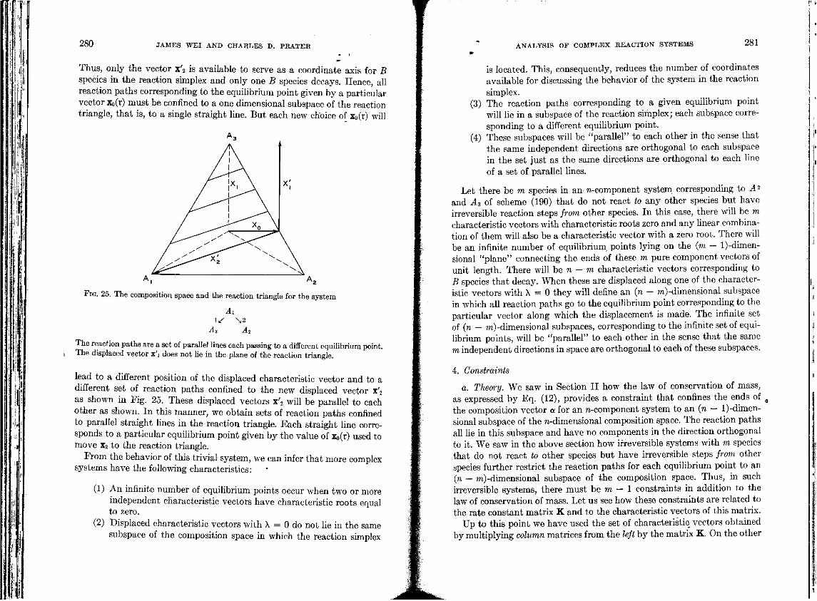
i
Eft
280 JAMES WEI AND CHARLES D. PRATER
Thus, only the vector x'2 is available to serve as a coordinate axis for B species in the reaction simplex and only one B species decays. Hence, all reaction paths corresponding to the equilibrium point given by a particular vector x0(r) must be confined to a one dimensional subspace of the reaction triangle, that is, to a single straight line. But each new choice of Xo(r) will
'1 "2 FIG. 25. The composition space and the reaction triangle for the system
-41
As A2
The reaction paths are a set of parallel lines each passing to a different equilibrium point, i The displaced vector x'i does not lie in the plane of the reaction triangle.
lead to a different position of the displaced characteristic vector and to a different set of reaction paths confined to the new displaced vector x'2
as shown in Fig. 25. These displaced vectors x'2 will be parallel to each other as shown. In this manner, we obtain sets of reaction paths confined to parallel straight lines in the reaction triangle. Each straight line corresponds to a particular equilibrium point given by the value of Xo(r) used to move X2 to the reaction triangle.
From the behavior of this trivial system, we can infer that more complex systems have the following characteristics:
(1) An infinite number of equilibrium points occur when two or more independent characteristic vectors have characteristic roots equal to zero.
(2) Displaced characteristic vectors with X = 0 do not lie in the same subspace of the composition space in which the reaction simplex
ANALYSIS OF COMPLEX REACTION SYSTEMS 281
is located. This, consequently, reduces the number of coordinates available for discussing the behavior of the system in the reaction simplex.
(3) The reaction paths corresponding to a given equilibrium point will lie in a subspace of the reaction simplex; each subspace corresponding to a different equilibrium point.
(4) These subspaces will be "parallel" to each other in the sense that the same independent directions are orthogonal to each subspace in the set just as the same directions are orthogonal to each line of a set of parallel lines.
Let there be m species in an n-component system corresponding to A2
and As of scheme (190) that do not react to any other species but have irreversible reaction steps from other species. In this case, there will be m characteristic vectors with characteristic roots zero and any linear combination of them will also be a characteristic vector with a zero root. There will be an infinite number of equilibrium points lying on the (m — l)-dimen-sional "plane" connecting the ends of these m pure component vectors of unit length. There will be n — m characteristic vectors corresponding to B species that decay. When these are displaced along one of the characteristic vectors with A = 0 they will define an (n — m)-dimensional subspace in which all reaction paths go to the equilibrium point corresponding to the particular vector along which the displacement is made. The infinite set of (n — m)-dimensional subspaces, corresponding to the infinite set of equilibrium points, will be "parallel" to each other in the sense that the same m independent directions in space are orthogonal to each of these subspaces.
4. Constraints
a. Theory. We saw in Section II how the law of conservation of mass, as expressed by Eq. (12), provides a constraint that confines the ends of the composition vector a for an n-component system to an (n — l)-dimen-sional subspace of the n-dimensional composition space. The reaction paths all lie in this subspace and have no components in the direction orthogonal to it. We saw in the above section how irreversible systems with m species that do not react to other species but have irreversible steps from other species further restrict the reaction paths for each equilibrium point to an (n — m)-dimensional subspace of the composition space. Thus, in such irreversible systems, there must be m — 1 constraints in addition to the law of conservation of mass. Let us see how these constraints are related to the rate constant matrix K and to the characteristic vectors of this matrix.
Up to this point we have used the set of characteristic vectors obtained by multiplying column matrices from the left by the matrix K. On the other
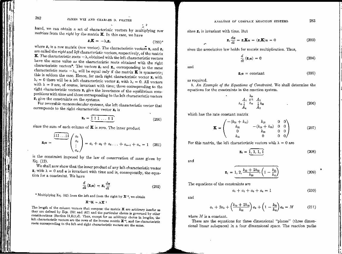
282 JAMES WEI AND CHARLES D. PRATER
hand, we can obtain a set of characteristic vectors by multiplying row matrices from the right by the matrix K. In this case, we have
ziK = -X.Z. (199)*
where zt- is a row matrix (row vector). The characteristic vectors X,- and z. are called the right and left characteristic vectors, respectively, of the matrix K. The characteristic roots —A, obtained with the left characteristic vectors have the same value as the characteristic roots obtained with the right characteristic vectors*. The vectors z, and x., corresponding to the same characteristic roots —A., will be equal only if the matrix K is symmetric; this is seldom the case. Hence, for each right characteristic vector x. with Xi = 0 there will be a left characteristic vector z. with A,- = 0. All vectors with A = 0 are, of course, invariant with time; those corresponding to the right characteristic vectors x, give the invariance of the equilibrium compositions with time and those corresponding to the left characteristic vectors z. give the constraints on the systems.
For reversible monomolecular systems, the left characteristic vector that corresponds to the right characteristic vector x0 is
Z0 = 1 1 1 . . . 1 1 (200)
since the sum of each column of K is zero. The inner product
Z0a = = ^ -f- a2 + a3. . . + an-X + an = 1 (201)
is the constraint imposed by the law of conservation of mass given by Eq. (12).
We shall now show that the inner product of any left characteristic vector %i with A = 0 and a is invariant with time and is, consequently, the equation for a constraint. We have
* Multiplying Eq. (62) from the left and from the right by X_I, we obtain
X-'K = AX"1
The length of the column vectors that compose the matrix X are arbitrary insofar as they are defined by Eqs. (59) and (62) and the particular choice is governed by other considerations (Section II,B,2,<2). Thus, except for an arbitrary choice in lengths, the left characteristic vectors are the rows of the inverse matrix X-1, and the characteristic roots corresponding to the left and right characteristic vectors are the same.
ANALYSIS OF COMPLEX REACTION SYSTEMS
since Z; is invariant with time. But
Z ; -^ = z tKa = (z,K)a = 0
since the associative law holds for matrix multiplication. Thus,
d
and
M <*"> " °
Ziff = constant
283
(203)
(204)
(205)
as required. b. An Example of the Equations of Constraint. We shall determine the
equations for the constraints in the reaction system.
hi Ai +± A2
hi i hi I ka , (206) At A3
which has the rate constant matrix
K =
ij + hi) hi 0
ku
kn — (kn + fc»)
k32
0
0 0 0 0
0 0 0 0,
(207)
For this matrix, the left characteristic vectors with A = 0 are
z0 = 1, 1, 1, 1
and
Zi = 1, 2, k12 + 2k
ho * v - c )
(208)
(209)
(210)
The equations of the constraints are
ai + a2 + a% -j- a4 = 1
and
0 l + 2 a , + ( f e + j * - ) a . + ( 1 _ g a . . J f ( 2 1 1 )
where M is a constant. These are the equations for three dimensional "planes" (three dimen
sional linear subspaces) in a four dimensional space. The reaction paths
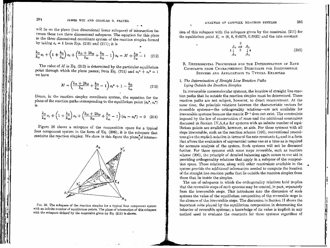
'«
M\
I I I
- r
284 JAMES WEI AND CHARLES D. PRATER
will lie on the plane (two dimensional linear subspace) of intersection between these two three dimensional subspaces. The equation for this plane in the three dimensional coordinate system of the reaction simplex formed by taking a4 = 1 from Eqs. (210) and (211); it is
E * + ( 1 + l S ) * + ( f e T r B + E - 1 ) - ' - J f + c l 1 ( 2 1 2 )
The value of M in Eq. (212) is determined by the particular equilibrium point through which the plane passes; from Eq. (211) and a3* + at* = 1 we have
M = _ (hi + 2fc32 , &21 _ , \ \ 32 h\ / «3* + 1 - £ i (213)
Hence, in the reaction simplex coordinate system, the equation for the plane of the reaction paths corresponding to the equilibrium point (a3*, a4*) is
O + f e M ^ + E - 1 ) ' * - ^ - 0 ™
Figure 26 shows a subspace of the composition space for a typical four component system in the form of Eq. (206); it is the subspace that contains the reaction simplex. We show in this figure the plane_of intersec-
FIG. 26. The subspace of the reaction simplex for a typical four component system with an infinite number of equilibrium points. The plane of intersection of this subspace with the subspace defined by the constraint given by Eq. (211) is shown.
ANALYSIS OF COMPLEX REACTION SYSTEMS 285
A. U A4
*--* 3
A2
i * Az
tion of this subspace with the subspace given by the constraint (211) for the equilibrium point ET = (0, 0, 0.6078, 0.3922) and the rate constant
(215)
B . EXPERIMENTAL PROCEDURES FOR THE DETERMINATION OF KATE
CONSTANTS FROM CHARACTERISTIC DIRECTIONS FOR IRREVERSIBLE
SYSTEMS AND APPLICATIONS TO TYPICAL EXAMPLES
1. The Determination of Straight Line Reaction Paths Lying Outside the Reaction Simplex
In irreversible monomolecular systems, the location of straight line reaction paths that lie outside the reaction simplex must be determined. These reaction paths are not subject, however, to direct measurement. At the same time, the principle relations between the characteristic vectors for reversible systems—the orthogonality relations—are not available for irreversible systems because the matrix D - 1 does not exist. The constraints imposed by the law of conservation of mass and the additional constraints discussed in Section IV,A,4,a for systems with an infinite number of equilibrium points are available, however, as aids. For those systems with all steps irreversible, such as the reaction scheme (166), conventional procedures give the explicit solution in terms of the rate constants kji and in a form that allows the evaluation of exponential terms one at a time as is required for accurate analysis of the system. Such systems will not be discussed further. For those systems with some steps reversible, such as reaction scheme (200), the principle of detailed balancing again comes to our aid in providing orthogonality relations that apply in a subspace of the composition space. These relations, along with other constraints available in the system provide the additional information needed to compute the location of the straight line reaction paths that he outside the reaction simplex from those that lie inside the simplex.
The use of subspaces in which the orthogonality relations hold implies that the reversible steps of such systems may be treated, in part, separately from the irreversible steps. This introduces into the discussion of such systems the value of the equilibrium composition of the reversible steps in the absence of the irreversible steps. The discussion in Section II shows tho important roles played by the equilibrium composition in determining the behavior of reversible systems; a knowledge of its value is implicit in any method used to evaluate the constants for these systems regardless of
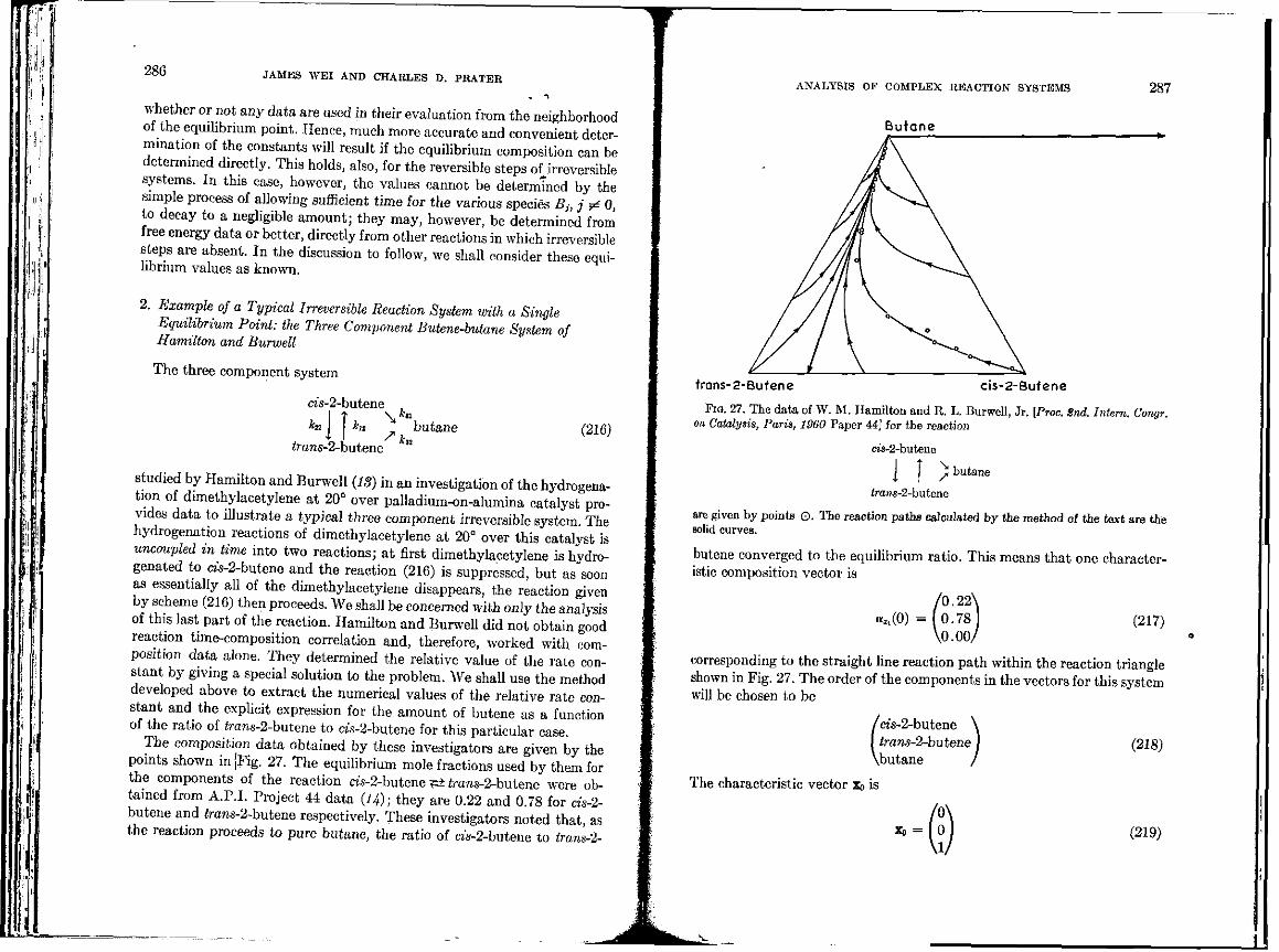
~ 1
286
i, .]
. 4
JAMES WEI AND CHARLES D. PRATER
whether or not any data are used in their evaluation from the neighborhood of the equilibrium point. Hence, much more accurate and convenient determination of the constants will result if the equilibrium composition can be determined directly. This holds, also, for the reversible steps of irreversible systems. In this case, however, the values cannot be determined by the simple process of allowing sufficient time for the various species Bj, j ^ 0, to decay to a negligible amount; they may, however, be determined from free energy data or better, directly from other reactions in which irreversible steps are absent. In the discussion to follow, we shall consider these equilibrium values as known.
2. Example of a Typical Irreversible Reaction System with a Single Equilibrium Point: the Three Component Butene-butane System of Hamilton and Rurwell
The three component system
m-2-butene
A*
irans-2-butene
butane (216)
studied by Hamilton and Burwell (IS) in an investigation of the hydrogena-tion of dimethylacetylene at 20° over palladium-on-alumina catalyst provides data to illustrate a typical three component irreversible system The hydrogenation reactions of dimethylacetylene at 20° over this catalyst is uncoupled in time into two reactions; at first dimethylacetylene is hydro-genated to as-2-butene and the reaction (216) is suppressed, but as soon as essentially all of the dimethylacetylene disappears, the reaction given by scheme (216) then proceeds. We shall be concerned with only the analysis of this last part of the reaction. Hamilton and Burwell did not obtain good reaction time-composition correlation and, therefore, worked with composition data alone. They determined the relative value of the rate constant by giving a special solution to the problem. We shall use the method developed above to extract the numerical values of the relative rate constant and the explicit expression for the amount of butene as a function of the ratio of tos-2-butene to cw-2-butene for this particular case.
The composition data obtained by these investigators are given by the points shown in (Fig. 27. The equilibrium mole fractions used by them for the components of the reaction tns-2-butene ^ iroTM-2-butene were obtained from A.P.I. Project 44 data (14); they are 0.22 and 0.78 for cis-2-butene and .rans-2-butene respectively. These investigators noted that, as the reaction proceeds to pure butane, the ratio of raa-2-butene to irans-2-
ANALYSIS OF COMPLEX REACTION SYSTEMS
Butane
287
trans-2-Butene cis-2-Butene
Fia. 27. The data of W. M. Hamilton and R. L. Burwell, Jr. [Proc. Snd. Intern. Congr. on. Catalysis, Paris, 1960 Paper 44] for the reaction
cxs-2-butene
I 1 \
frans-2-butene
butane
are given by points ©. The reaction paths calculated by the method of the text are the solid curves.
butene converged to the equilibrium ratio. This means that one characteristic composition vector is
/0.22^ ««(0) = 0 . 7 8
\0.00> (217)
corresponding to the straight line reaction path within the reaction triangle shown in Fig. 27. The order of the components in the vectors for this system will be chosen to be
/m-2-butene \ I frans-2-butene I \butane /
The characteristic vector Xo is
(218)
(219)
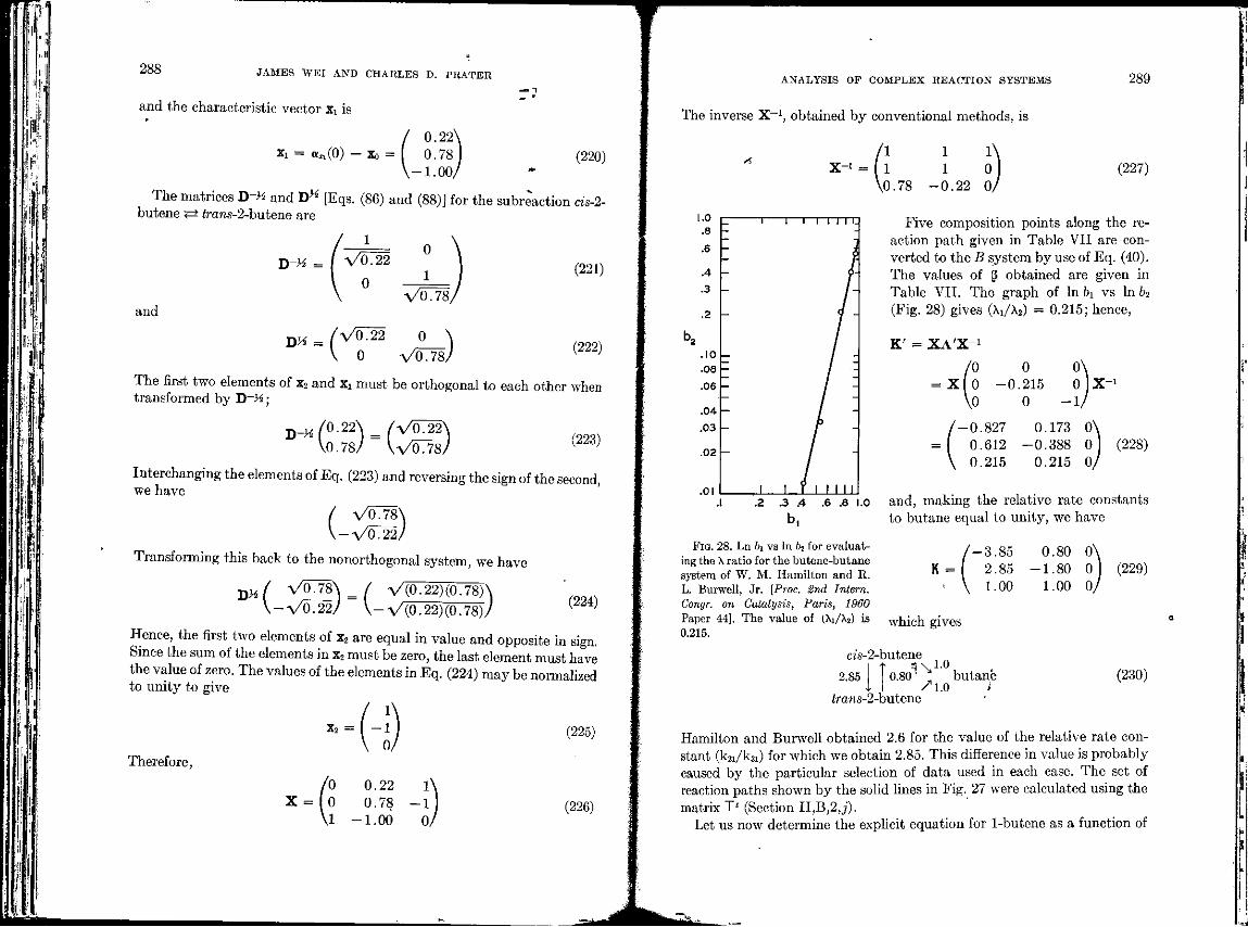
M •
I I-
\W
\ •:
288 JAMES WEI AND CHARLES D. PRATER -_.-?
and the characteristic vector Xi is
/ 0.22\ Xi = a«(0) - X o = 0.78 (220)
\ - 1 . 0 0 /
The matrices D>- and D H [Eqs. (86) and (88)] for the subreaction cis-2-butene <= trans-2~butene are
and
D M =
D ^ =
Vo778,
0.22 0 N
0 V0778,
(221)
(222)
The first two elements of x2 and Xi must be orthogonal to each other when transformed by D_H;
jy-H 0.22 ,0.78 (223)
Interchanging the elements of Eq. (223) and reversing the sign of the second, we have
. - A / 0 . 2 2 ,
Transforming this back to the nonorthogonal system, we have
W V ( L T 8 W V(0.22)(0.78)\ " V - V 0 T 2 2 / V-V(0 .22 ) (0 .78 ) /
Hence, the first two elements of x2 are equal in value and opposite in sign. Since the sum of the elements in x2 must be zero, the last element must have the value of zero. The values of the elements in Eq. (224) may be normalized to unity to give
x2 = f - 1 j (225)
Therefore,
/0 0.22 l \ X = (0 0.78 - l ) (226)
\ 1 - 1 . 0 0 0 /
ANALYSIS OF COMPLEX REACTION SYSTEMS 289
The inverse X"1, obtained by conventional methods, is
X-1 = n 1 V 1 1 0
V0.78 - 0 . 2 2 0/ (227)
Five composition points along the reaction path given in Table VII are converted to the B system by use of Eq. (40). The values of § obtained are given in Table VII. The graph of In 6_ vs In b2
(Fig. 28) gives (X_/Aa) = 0.215; hence,
K' = XA'X" 1
' - 0 . 8 2 7 0.173 0.612 - 0 . 3 8 8
. 0.215 0.215 (228)
.8 1.0
Fia. 28. Ln f»i vs In h for evaluating the X ratio for the butene-butane system of W. M. Hamilton and R. L. Burwell, Jr. [Proc. 2nd Intern. Congr. on Catalysis, Paris, 1960 Paper 44]. The value of (Xi/X_) is 0.215.
and, making the relative rate constants to butane equal to unity, we have
K =
which gives
0.80 0N
-1.80 0 1.00 0;
(229)
ezs-2-butene sj^l.0
2.85 I
frans-2-butene
0.80 - "" butane / l .O #
(230)
Hamilton and Burwell obtained 2.6 for the value of the relative rate constant (k2i/k3i) for which we obtain 2.85. This difference in value is probably caused by the particular selection of data used in each case. The set of reaction paths shown by the solid lines in Fig.^27 were calculated using the matrix T ( (Section II,B,2j).
Let us now determine the explicit equation for 1-butene as a function of
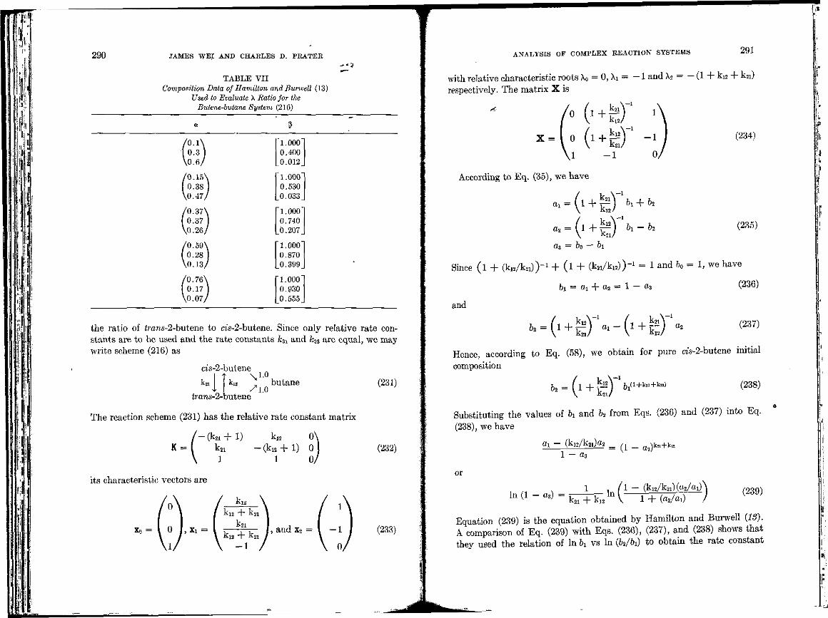
I
290 JAMES WEI AND CHARLES D. PRATER
TABLE VII Composition Data of Hamilton and Burwell (13)
Used to Evaluate X Ratio for the Butene-butane System (216)
_*
ft.l\ 0.3 J
V0.6/
/0.15s
0.38 V0.47,
'0.37s
0.37 ^0.26,
0.59s
0.28 0.13;
'0.76^ 0.17
O).07,
the ratio of irans-2-butene to m-2-butene. Since only relative rate constants are to be used and the rate constants hi and k32 are equal, we may write scheme (216) as
cis-2-butene
frans-2-butene
\ i . o
/•i.o butane (231)
The reaction scheme (231) has the relative rate constant matrix
K =
its characteristic vectors are
,Xi =
k12 0 (ku-r - l ) 0
1 0> (232)
kw + k n
k2i
k12 + k2i
- 1
!, and x2 = (233)
ANALYSIS OF COMPLEX REACTION SYSTEMS 291
with relative characteristic roots A0 = 0, A. = - 1 and A2 = - (1 + ki2 -f k_i) respectively. The matrix X is
(234)
- 1
According to Eq. (35), we have
- - ( i + f e T f c - f c (235)
a3 = bo — bi
Since ( l + ( W k . . ) ) - 1 + C1 + ( W k w ) ) " 1 = 1 and b0 = 1, we have
^ = ai + a2 = 1 - o> (236)
and
» . - v + _ s r * - v + E r * ( 2 3 7 )
Hence, according to Eq. (58), we obtain for pure ras-2-butene initial
composition
fc-(i+E_;rw,+ta +ka) (238)
Substituting the values of &_ and b2 from Eqs. (236) and (237) into Eq.
(238), we have
a. — (ki2/k2i)aa _ n __ a \k_i+kL_ 1 — a3
, „ ^ I 1 f1 ~ (kl2/k21) (02/^1)^ (2oq) 111 ( 1 " ^ " E T + k i l n I 1 + (a,/ai) ) ( 2 3 9 )
Equation (239) is the equation obtained by Hamilton and Burwell IS). A comparison of Eq. (239) with Eqs. (236), (237), and (238) shows that they used the relation of ln 61 vs ln (b2/bi) to obtain the rate constant
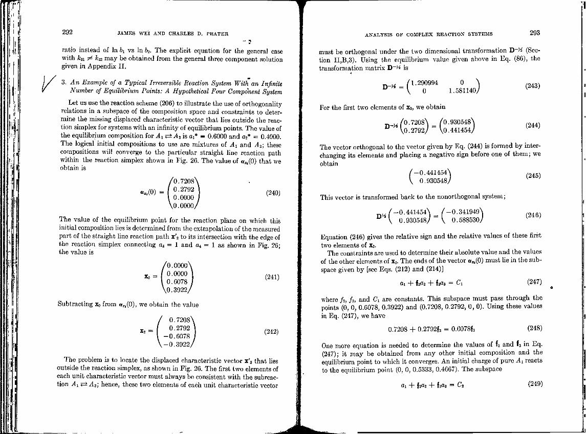
Ki t
292 JAMES WEI AND CHARLES D. PRATER
ratio instead of ln &x vs ln b2. The explicit equation for the general case with kn 5 32 may be obtained from the general three component solution given in Appendix II.
3. An Example of a Typical Irreversible Reaction System With an Infinite Number of Equilibrium Points: A Hypothetical Four Component System
Let us use the reaction scheme (206) to illustrate the use of orthogonality relations in a subspace of the composition space and constraints to determine the missing displaced characteristic vector that lies outside the reaction simplex for systems with an infinity of equilibrium points. The value of the equilibrium composition for Ai +± A2 is ai* = 0.6000 and a2* = 0.4000. The logical initial compositions to use are mixtures of Ai and A2; these compositions will converge to the particular straight line reaction path within the reaction simplex shown in Fig. 26. The value of a*.(0) that we obtain is
*-_(0) =
'0.7208 0.2792 0.0000
,0.0000,
(240)
The value of the equilibrium point for the reaction plane on which this initial composition lies is determined from the extrapolation of the measured part of the straight line reaction path x'2 to its intersection with the edge of the reaction simplex connecting a3 = 1 and a4 = 1 as shown in Fig. 26; the value is
Xo =
'0.0000 0.0000 0.6078
,0.3922,
(241)
Subtracting Xo from orXl(0), we obtain the value
x2 =
0.7208 0.2792
-0 .0078 -0 .3922,
(242)
The problem is to locate the displaced characteristic vector x'3 that lies outside the reaction simplex, as shown in Fig. 26. The first two elements of each unit characteristic vector must always be consistent with the subreac-tion Ai +± A2; hence, these two elements of each unit characteristic vector
T
ANALYSIS OF COMPLEX REACTION SYSTEMS 293
must be orthogonal under the two dimensional transformation D - ^ (Section II,B,3). Using the equilibrium value given above in Eq. (86), the transformation matrix D~>* is
D - X - f -290994
0 0
1.581140 )
For the first two elements of x2, we obtain
A).7208\ _ A).930548\ VO.2792/ ~ \0.441454/
(243)
(244)
The vector orthogonal to the vector given by Eq. (244) is formed by interchanging its elements and placing a negative sign before one of them; we obtain
' -0 .441454\ 0.930548/ (
(245)
This vector is transformed back to the nonorthogonal system;
nH / - 0 . 4 4 1 4 5 4 \ = / - 0 . 3 4 1 9 4 9 \ \ 0.930548/ V 0.588530/
(246)
Equation (246) gives the relative sign and the relative values of these first two elements of X3.
The constraints are used to determine their absolute value and the values of the other elements of X3. The ends of the vector a*,(0) must lie in the sub-space given by [see Eqs. (212) and (214)]
a. + f2a2 + \zaz = C\ (247)
where f2, f3, and C. are constants. This subspace must pass through the points (0, 0, 0.6078, 0.3922) and (0.7208, 0.2792, 0, 0). Using these values in Eq. (247), we have
0.7208 + 0.2792f2 = 0.6078f3 (248)
One more equation is needed to determine the values of f2 and U in Eq. (247); it may be obtained from any other initial composition and the equilibrium point to which it converges. An initial charge of pure A. reacts to the equilibrium point (0, 0, 0.5333, 0.4667). The subspace
a. + f2«2 + isO-i = C2 (249)
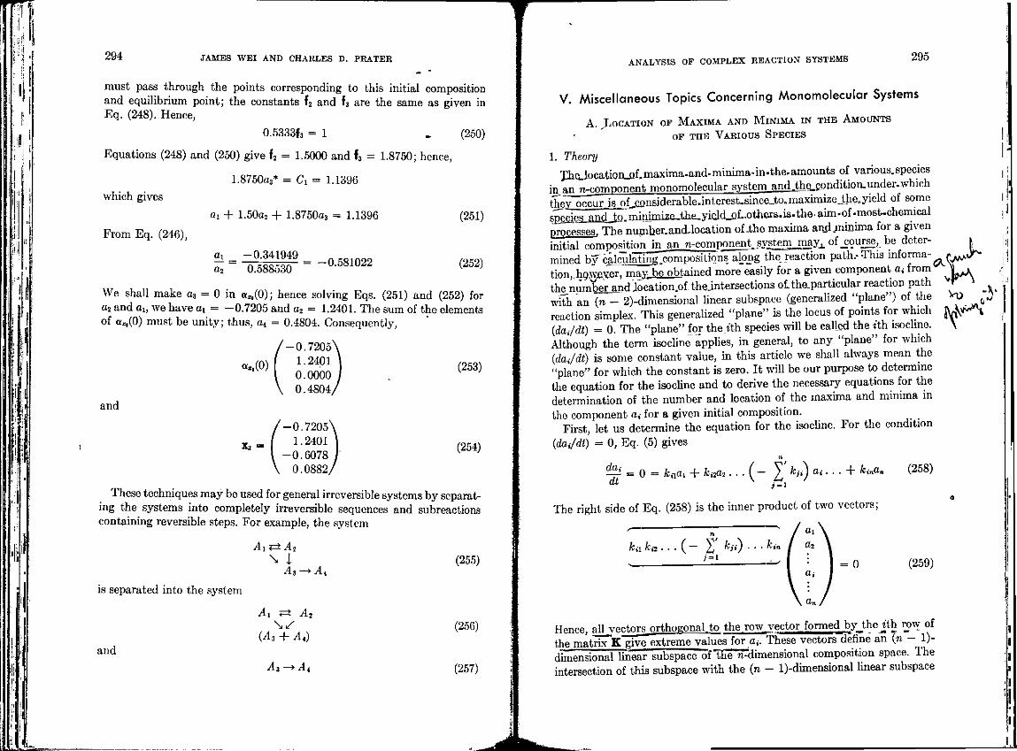
m
T
294 JAMES WEI AND CHARLES D. PRATER
must pass through the points corresponding to this initial composition and equilibrium point; the constants f2 and f3 are the same as given in Eq. (248). Hence,
0.5333f3 = 1 » (250)
Equations (248) and (250) give f2 = 1.5000 and f3 = 1.8750; hence,
1.8760a,* = Ci = 1.1396
which gives
From Eq. (246),
a. + 1.500s -I- 1.8760oj = 1.1396
ai = -0.341949 a2 0.588530
= -0.581022
(251)
(252)
We shall make o3 = 0 in a^O); hence solving Eqs. (251) and (252) for a2 and a_, we have a. = —0.7205 and a2 = 1.2401. The sum of the elements of aj:.(0) must be unity; thus, a4 = 0.4804. Consequently,
«*.(0)
and
x> =
- 0 . 7 2 0 5 \ 1.2401 I 0.0000 / 0.4804/
-0 .7205 1.2401
-0 .6078 0.0882,
(253)
(254)
These techniques may be used for general irreversible systems by separating the systems into completely irreversible sequences and subreactions containing reversible steps. For example, the system
is separated into the system
and
Ai^±A2
\ I A3-»_44
A, <=fc A2
(A3 + A4)
A4
(255)
(256)
(257)
ANALYSIS OP COMPLEX REACTION SYSTEMS 295
V. Miscellaneous Topics Concerning Monomolecular Systems
A. ..LOCATION OF MAXIMA AND MINIMA IN THE AMOUNTS
OP THE VARIOUS SPECIES
1. Theory Tiiejocatiori_j)f_maxima.and.minima-in-the-amounts of various.species
in an n-component monomolecular system and_thQ_cpadit.on.under-which they oc^cur.is_of_cj)nsiderable.interest,since_to„maximize_the„yield of some sj*^ej_jmg__ia. minimi_.e-.the. y ieJdj_)f..others.is-the-aim-of-most-chemical processes. The number.and-location of .the maxima and minima for a given initial composition in an n-component. systemmayj, of course, be determined by calculating ..compositions along the_ reaction path.-This information,, hpy^eyer, may, be obtained more easily for a given component a. from the number_and Jocation.of thejntersections of_the_particular reaction path with an (n — 2)-dimensional linear subspace (generalized "plane") of the reaction simplex. This generalized "plane" is the locus of points for which (dcti/dt) = 0. The "plane" for the.ith species will be called the ith isocline. Although the term isocline applies, in general, to any "plane" for which (dtti/dt) is some constant value, in this article we shall always mean the "plane" for which the constant is zero. I t will be our purpose to determine the equation for the isocline and to derive the necessary equations for the determination of the number and location of the maxima and minima in the component a,- for a given initial composition.
First, let us determine the equation for the isocline. For the condition
(dai/dt) = 0, Eq. (5) gives
* » o"
n
= 0 = knai + ki2a2. • . ( — \ kit\ a. . . -f fcina,
The right side of Eq. (258) is the inner product of two vectors;
dot dt
(258)
knki2...(- t * * ) • • • *
= 0 (259)
Hence, allvectors^rthogonal.to the row^yectqr formed by the ith row of the matrix K give extreme values for a.. These vectors define an (n — 1)-dimensional linear subspace of "the ^"dimensional composition space. The intersection of this subspace with the (n — l)-dimensional linear subspace
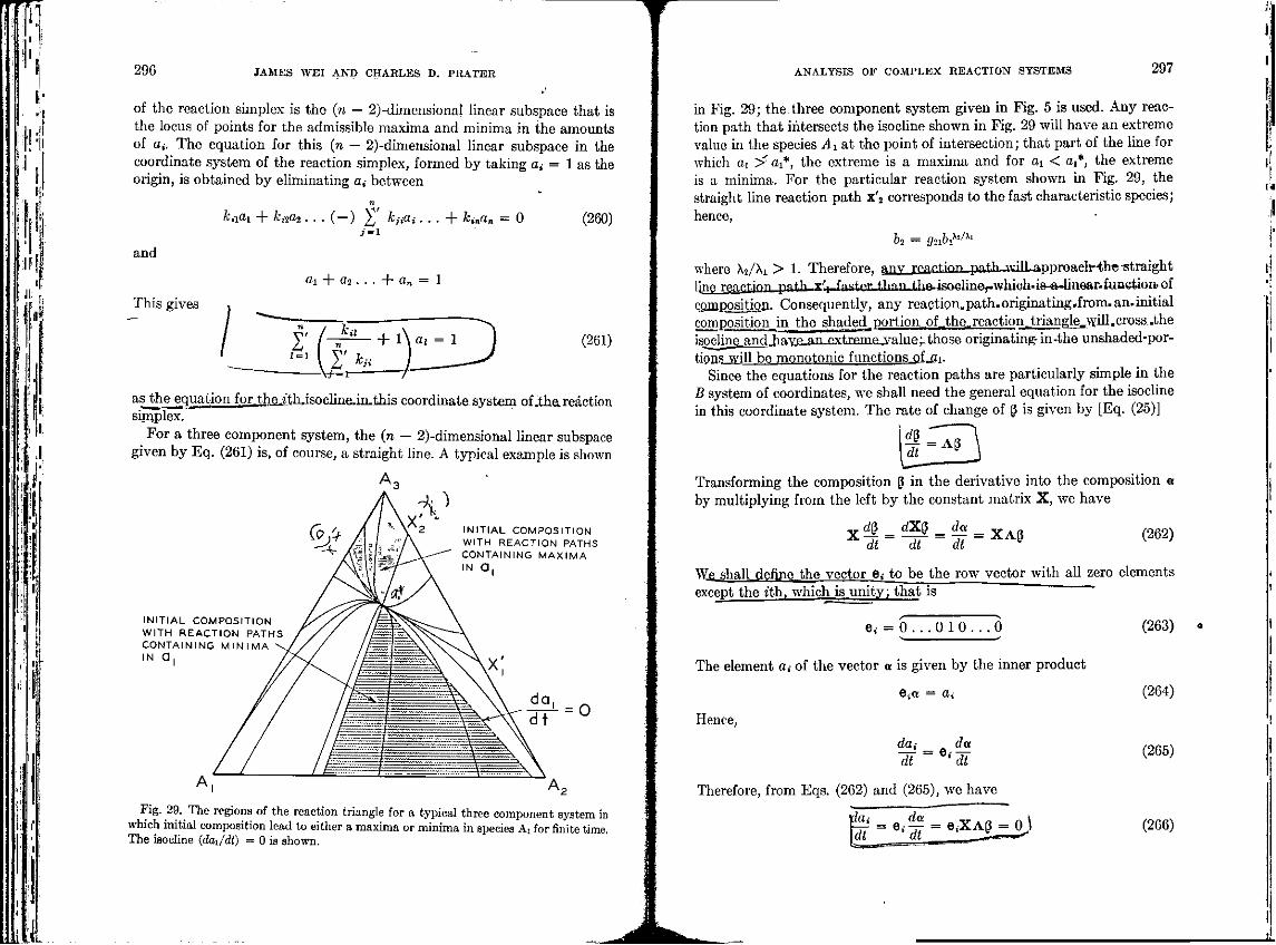
M
'»!
290 JAMES WEI AND CHARLES D. PRATER
of the reaction simplex is tho (n — 2)-dimensional linear subspace that is the locus of points for the admissible maxima and minima in the amounts of a.. The equation for this (n — 2)-dimensional linear subspace in the coordinate system of the reaction simplex, formed by taking a, = 1 as the origin, is obtained by eliminating a,- between
and
This gives
hi^ + ki2a2...(-) J ' kjiai... 4- kinan = 0 (260)
«i + a2. . . -f an = 1
ku y
Vwi
+ l \ a . = 1 (261)
as the equation for theith.isocline.in.this coordinate system of.the.reaction sirnplex.
For a three component system, the (n — 2)-dimensional linear subspace given by Eq. (261) is, of course, a straight line. A typical example is shown
A 3
A '
-A INITIAL COMPOSITION WITH REACTION PATHS CONTAINING MAXIMA IN a,
INITIAL COMPOSITION WITH REACTION PATHS CONTAINING MINIMA IN a.
I _ = 0
Fig. 29. The regions of the reaction triangle for a typical three component system in which initial composition lead to either a maxima or minima in species Ai for finite time, The isocline (dai/dt) — 0 is shown.
I
ANALYSIS OF COMPLEX REACTION SYSTEMS 297
in Fig. 29; the three component system given in Fig. 5 is used. Any reaction path that intersects the isocline shown in Fig. 29 will have an extreme value in the species Ai at the point of intersection; that part of the line for which ai ~> a_*, the extreme is a maxima and for a. < ai*, the extreme is a minima. For the particular reaction system shown in Fig. 29, the straight line reaction path x'2 corresponds to the fast characteristic species; hence,
b2 = g2ibi*/Xl
where X2/Xi > 1. Therefore, any reaction p.it.h-ivilLn.pprna.ffTi-t.hft-straight. line reaction pat-h yft-f»qt^r ^ ^ t.hA^sar^.linAriHhinh..ft^inrar.f-inatinn.nf c5lBB0si$isii. Consequently, any reaction.path.originating.from-an-initial composition_in the shaded, portion .of..the., reaction. triangle^Y-ll. cross -the isocline and iiaY£jm_£xtremeuyalue^ those originating-in-the unshaded-por-tions will be monotonic functions.of._3i.
Since the equations for the reaction paths are particularly simple in the B system of coordinates, we shall need the general equation for the isocline in this coordinate system. The rate of change of (J is given by [Eq. (25)]
Transforming the composition g in the derivative into the composition a by multiplying from the left by the constant matrix X, we have
dt dt dt (262)
We shall define the vector e. to be the row vector with all zero elements except the t'th, which is unity; that is
e, = 0 . . . 0 1 0 . . . 0
The element a,- of the vector a is given by the inner product
e.a = ai
Hence,
da* _ da It " 'It
Therefore, from Eqs. (262) and (265), we have
iai da _ Y *« n \
(263)
(264)
(265)
(266)
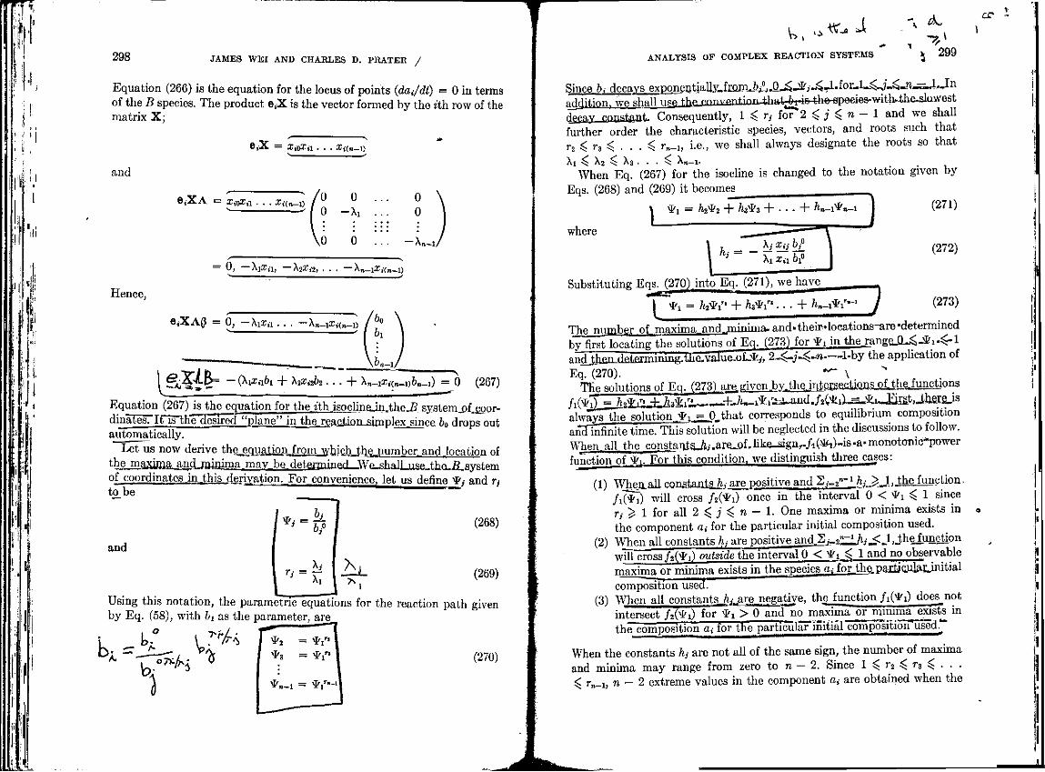
If / I :i a ,
I I
T
298 JAMES WEI AND CHARLES D. PRATER /
Equation (266) is the equation for the locus of points (dai/dt) = 0 in terms of the B species. The product e.X is the vector formed by the ith row of the matrix X;
e,X = XidXn .. . £.(n_i
and
e.XA = XioXa . . . Xi(n-i) 0 0
— An-1
— 0, —XiXn, —X2xi2, . . . — X-.-.rEtfn-i)
Hence,
CXA0 = 0, -XiXfl . . . -Xn-iXifn-l) / & 0
Oi
._ sjgr1- -£ - X A B = -(Xixabi 4- X2xi2b2. . . + X»-1a;«1_,)6B_i) = 0 (267)
Equation (267) is the equation for the ith jsocIine_in.theJ? systemj>f.£Qor-dinatesl"IfTis~thTo!esired "plane" in the reaciion^simplex.since 60 drops out automatically.
Let us now derive thej^quat.ion.frQm which _the„numbcr and .location of the maxima andjn.rt.ima may be_determinej_l^We^halLuseL.the.-5-Svstem of coordinates in .this dgriyation._For convenience, let us define ¥,• and Tj to be
and
" " £ A
(268)
(269)
Using this notation, the parametric equations for the reaction path given by Eq. (58), with bt as the parameter, are.
V Thh
-A. — r ^ - "&
1
(270)
"tf_is -A
ANALYSIS OF COMPLEX REACTION SYSTEMS
\ (^
^
i 299
Since &,- decays exDonentiaUv-from.o,^.O^J&,j^_J.foi^I-^-i-^-n_-^iJ-In a^lgUl_igji^jv^jyiji^^ decay constant. Consequently, 1 ^ Tj for 2 ^ j ^ n —• 1 and we shall further order the characteristic species, vectors, and roots such that i"2 ^ r3 ^ . . . ^ r„_i, i.e., we shall always designate the roots so that Xi $ \2 5; X; ^ Xn_L
When Eq. (267) for the isocline is changed to the notation given by Eqs. (268) and (269) it becomes
x * . = k&t + h^fi + . . . + /ln-l*«_l j (271)
where
I
i. - _ hBi'PI
Substituting Eqs. (270)_into Eq. (271), we have
* ! = A2*iri + A»*iri • • • + ^n-i*ir""' L
(272)
(273)
The number of maxima and_jninima. and* their*locations-are -determined by first locating the solutions of Eq. (273)Jor SP. in the.range_Q_j$Jfc.-^"l anq^b___ii_dei1exminhig.the.viJue,of-_14'-y, 2^-j^-n—1-by the application of Eq. (270). — v
The solutions of Eq. (273)^^.given,by..the.i^terjjejjlon.s_oLthe.functions /i(%) = MfriV+.ftig.l. . + J ^ i * r ^ ^ n d _ / 2 C * i ) ^ J t i ^ r i t ) J h e j s J s always the solution tyi = 0 that corresponds to equilibrium composition antTinfinite time. This solution will be neglected in the discussions to follow. When., all the constants^,-.are>oi.hke_signr./i(*i)--is-a-monotonic"power function of ffj. For this condition, we distinguish three cases:
(1) WhejLali constants,^ are positive and _SJ_2"~1 Aj._5r__l, jbhejunction,
/ i (*i) will cross /2(*i) once in the interval 0 < ^ i ^ 1 since ry ^ 1 for all 2 ^ j ^ n — 1. One maxima or minima exists in the component a,- for the particular initial composition used.
(2) When all constants hj are positive and_Sj,_._^i/t,-_<. J ,_lhejunctipn will c r o s s / ^ i ) outside the interval 0 < ^ i ^ 1 and no observable maxima or minima exists in the species a. forthe. par4jc_ularjnitial composition used.
(3) When all constants_/ij„are_negatiye, the function / i ^ i ) does not intersect /a(*0 for ^ i > 0 and no maxima or minima exists in the composition a. for the particulaTinitialTomp^'sition'used•*""
When the constants hj are not all of the same sign, the number of maxima and minima may range from zero to n — 2. Since 1 ^ r2 ^ r8 ^ . . . ^ r„_i, n — 2 extreme values in the component a,- are obtained when the
cc*
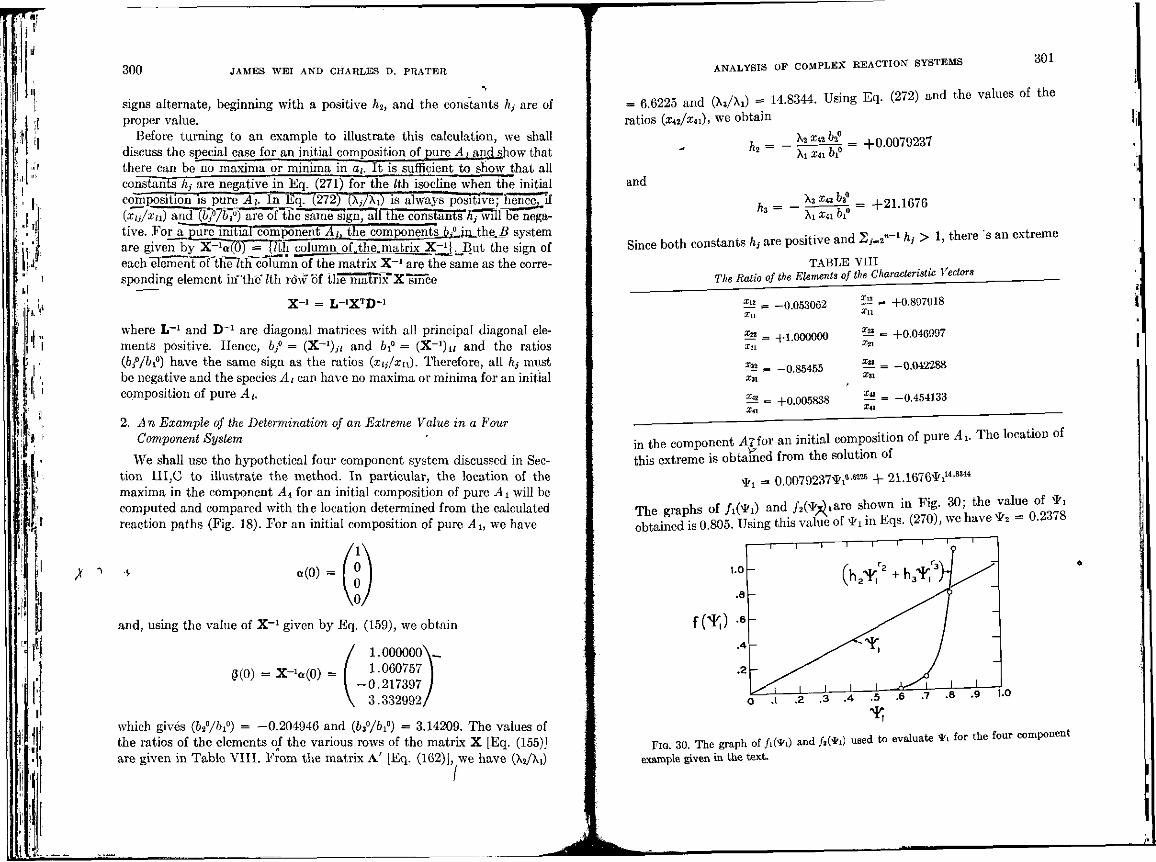
h • i _t
ii i
300 JAMES WEI AND CHARLES D. PRATER
signs alternate, beginning with a positive h2, and the constants hj are of proper value.
Before turning to an example to illustrate this calculation, we shall discuss the special case for an initial composition of pure At and show that there can be no maxima or minima in a. I t is sufficient to show that all constants hj are negative in Eq. (271) for the Ith isocline when the initial composition is pure _4[. In Eq. (272) (Xj/X.) is always positive; henc'e^if (xij/xij) and ~Qfj0'/b~i0) are of the same sign^'alf the constants ft/will be negative. For impure initial component -4f__the components_ijilia_.the.i? system are given by X~]c.(0) == j/th column, of„the.n_atrix X^'J._But the sign of each Element of the lih column of the matrix X _ I are the same as the corresponding element in'the ith row of the"matrix"X"since
X 1 = L - ^ D - 1
where L_ 1 and D*1 are diagonal matrices with all principal diagonal elements positive. Hence, 6/ = (X^1);. and hi" = (X - 1)^ and the ratios (bj°/bi°) have the same sign as the ratios (xij/xii). Therefore, all hj must be negative and the species Ac can have no maxima or minima for an initial composition of pure A...
2. An Example of the Determination of an Extreme Value in a Four Component System
We shall use the hypothetical four component system discussed in Section III,C to illustrate the method. In particular, the location of the maxima in the component A4 for an initial composition of pure Ai will be computed and compared with the location determined from the calculated reaction paths (Fig. 18). For an initial composition of pure Au we have
«(0) =
and, using the value of X - 1 given by Eq. (159), we obtain
3(0) = x - ^ o ) =
1.000000 1.060757
-0.217397 3.332992;
which gives (&.°/&i°) = -0.204946 and (63°/6i°) = 3.14209. The values of the ratios of the elements of the various rows of the matrix X [Eq. (155)] are given in Table VIII. From the matrix A ' [Eq. (162)], we have (X2/X.)
T
ANALYSIS OF COMPLEX REACTION SYSTEMS 301
= 6.6225 and (X3/X_) == 14.8344. Using Eq. (272) and the values of the
ratios (xi2/xu), we obtain
X2 xi2 62° h,= - Xi X41 &1°
l- = +0.0079237
and
h h Xi3 bi° = +21.1676 hz~ XiXab?
Since both constants h, are positive and S ^ - ' ht > 1, there s an extreme
TABLE VIII The Ratio of the Elements of the Characteristic Vectors
Ei? _= -0.053062
^ - +1.000000 X_i ^ = -0.85455 2.1
^ = +0.005838 Xn
Xiz xn
= +0.897018
^ = +0.046997 #21 ?* 0.042288 ZJI
H 0.454133 x«
in the component Atfor an initial composition of pure A , The location of
this extreme is obtained from the solution of
* ! = 0.0079237*!8-8225 + 21.1676*!14-8344
The graphs of /_(*_) and / 2 ( ^ . a r e shown in Fig. 30 the value of * obtained is 0.805. Using this value of *_ in Eqs. (270), we have * 2 = 0.2378
f(%) - 6 "
O .1 .2 -3 -4 ~£& n .e .9 '-0
FIG. 30. The graph of /.(*_) and /,(*0 used to evaluate *. for the four component example given in the text.
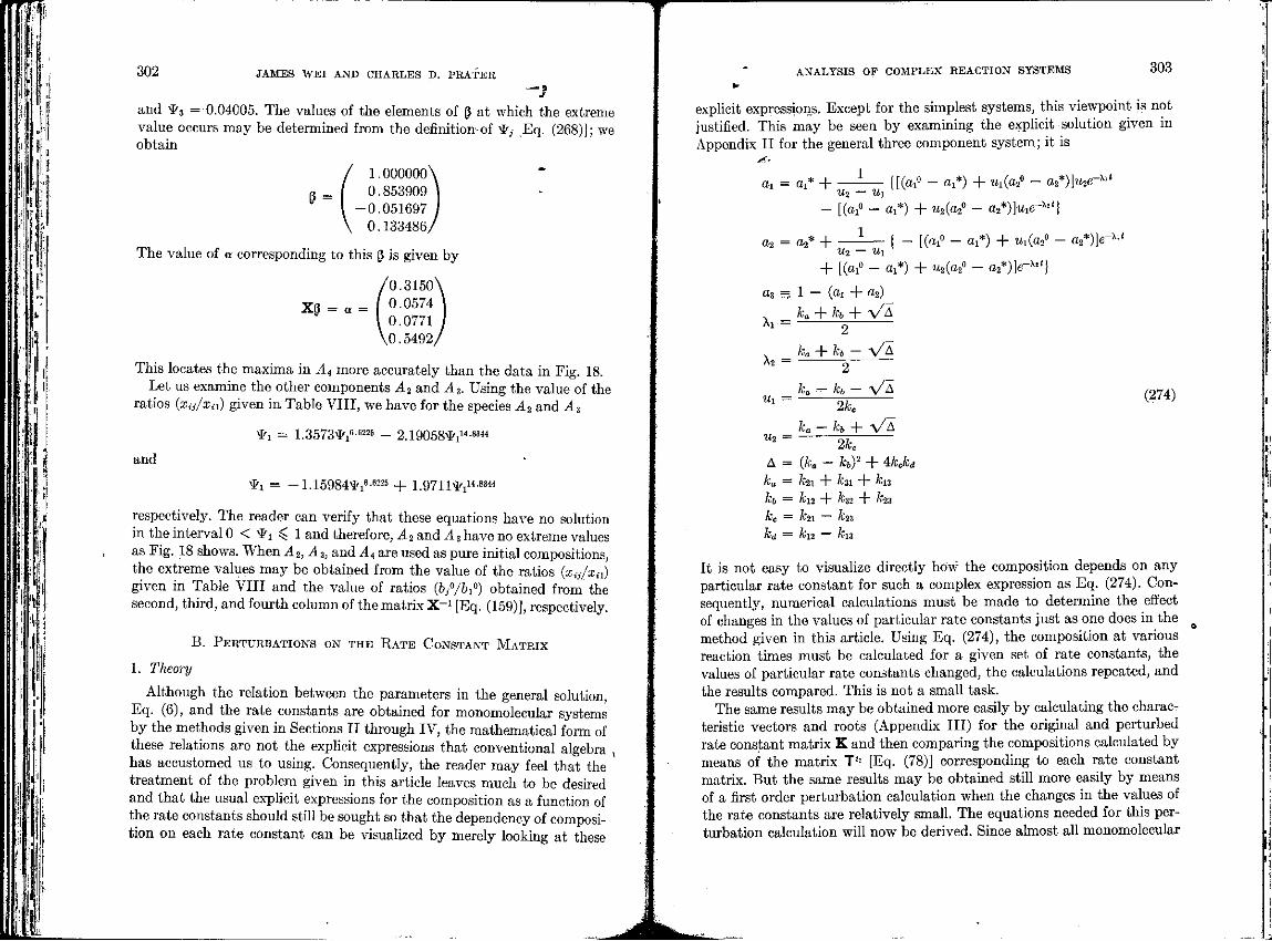
i l l
m
302 JAMES WEI AND CHARLES D. PRATER S
and ^3 = 0.04005. The values of the elements of (3 at which the extreme value occurs may be determined from the definition of >_>, Eq. (268)]; we obtain
0 =
1.000000\ 0.853909 \
-0.051697 j 0.133486/
The value of « corresponding to this ( is given by
(0-3150\ 0.0574 0.0771 J 0.5492/
This locates the maxima in A\ more accurately than the data in Fig. 18. Let us examine the other components A2 and As. Using the value of the
ratios (xij/xa) given in Table VIII, we have for the species A2 and A3
and
* i = 1.3573*!6 622B - 2.19058^i14-83«
* ! = -1.15984-*!6-6225 + 1.9711*i"-««
respectively. The reader can verify that these equations have no solution in the interval 0 < ^ i ^ 1 and therefore, A2 and A 3 have no extreme values as Fig. 18 shows. When A2, A3l and AA are used as pure initial compositions, the extreme values may be obtained from the value of the ratios (xij/xn) given in Table VIII and the value of ratios (bj°/bi°) obtained from the second, third, and fourth column of the matrix X - 1 [Eq. (159)], respectively.
B . PERTURBATIONS ON THE RATE CONSTANT MATRIX
1. Theory
Although the relation between the parameters in the general solution, Eq. (6), and the rate constants are obtained for monomolecular systems by the methods given in Sections II through IV, the mathematical form of these relations are not the explicit expressions that conventional algebra has accustomed us to using. Consequently, the reader may feel that the treatment of the problem given in this article leaves much to be desired and that the usual explicit expressions for the composition as a function of the rate constants should still be sought so that the dependency of composition on each rate constant can be visualized by merely looking at these
ANALYSIS OF COMPLEX REACTION SYSTEMS 303
explicit expressions. Except for the simplest systems, this viewpoint is not justified. This may be seen by examining the explicit solution given in Appendix II for the general three component system; it is
ai = a_* + 1 [(ai° -fl i*) +w_(a 2 ° - a2*)]u_e ,-\it
U2 — U\ - [(a.0 - a_*) + u2(a2° - a2*)He-X2'j
a2 = a2* + - [(oi° - a^) + Ui(a2° - a2*)\e~^ u2 — Ui
+ [(a!0 - a:*) + u2(a2° - a2*)]<r-*"
a3 = 1 - (a_ + a2)^
, ka + kb + V A
AI =
X2 =
Ml
Us =
ka
Ka
rCa
2
+ h -2
— kb — 2h
- h +
V A
V A
V A
(274)
2h A = (ka - kbf + ±kckd
ka - hi + kn + kl3
h = h2 + &32 + 23 ke = kn — &23 kd = kl2 — ku
It is not easy to visualize directly how the composition depends on any particular rate constant for such a complex expression as Eq. (274). Consequently, numerical calculations must be made to determine the effect of changes in the values of particular rate constants just as one does in the method given in this article. Using Eq. (274), the composition at various reaction times must be calculated for a given set of rate constants, the values of particular rate constants changed, the calculations repeated, and the results compared. This is not a small task.
The same results may be obtained more easily by calculating the characteristic vectors and roots (Appendix III) for the original and perturbed rate constant matrix K and then comparing the compositions calculated by means of the matrix T'1 [Eq. (78)] corresponding to each rate constant matrix. But the same results may be obtained still more easily by means of a first order perturbation calculation when the changes in the values of the rate constants are relatively small. The equations needed for this perturbation calculation will now be derived. Since almost all monomolecular

![OPEN ACCESS entropy · 2011. 5. 23. · Lumping analysis aims to combine reagents into “quasicomponents” for dimension reduction [15,17–19]. Wei and Prater [16] demonstrated](https://static.fdocuments.us/doc/165x107/60e7091d3b541240f85ae617/open-access-2011-5-23-lumping-analysis-aims-to-combine-reagents-into-aoequasicomponentsa.jpg)