Web-scale Multimedia Search for Internet Video Contentlujiang/resources/ThesisProposal.pdf ·...
112
CARNEGIE MELLON UNIVERSITY Web-scale Multimedia Search for Internet Video Content by Lu Jiang Ph.D Thesis Proposal Thesis Committee: Dr. Alex Hauptmann, Carnegie Mellon University Dr. Teruko Mitamura, Carnegie Mellon University Dr. Louis-Philippe Morency, Carnegie Mellon University Dr. Tat-Seng Chua, National University of Singapore Language Technologies Institute October 2015
Transcript of Web-scale Multimedia Search for Internet Video Contentlujiang/resources/ThesisProposal.pdf ·...
CARNEGIE MELLON UNIVERSITY
Web-scale Multimedia Search for
Internet Video Content
by
Lu Jiang
Ph.D Thesis Proposal
Thesis Committee:
Dr. Alex Hauptmann, Carnegie Mellon University
Dr. Teruko Mitamura, Carnegie Mellon University
Dr. Louis-Philippe Morency, Carnegie Mellon University
Dr. Tat-Seng Chua, National University of Singapore
Language Technologies Institute
October 2015

Abstract
The Internet has been witnessing an explosion of video content. According to a Cisco
study, video content accounted for 64% of all the world’s internet traffic in 2014, and
this percentage is estimated to reach 80% by 2019. Video data are becoming one of
the most valuable sources to assess information and knowledge. However, existing video
search solutions are still based on text matching (text-to-text search), and could fail for
the huge volumes of videos that have little relevant metadata or no metadata at all. The
need for large-scale and intelligent video search, which bridges semantic gap between the
user’s information need and the video content, seems to be urgent.
In this thesis, we propose an accurate, efficient and scalable search method for video
content. As opposed to text matching, the proposed method relies on automatic video
content understanding, and allows for intelligent and flexible search paradigms over the
video content (text-to-video and text&video-to-video search). It provides a new way
to look at content-based video search from finding a simple concept like “puppy” to
searching a complex incident like “a scene in urban area where people running away after
an explosion”. To achieve this ambitious goal, we propose several novel methods focusing
on accuracy, efficiency and scalability in the novel search paradigm. First, we introduce
a novel self-paced curriculum learning theory that allows for training more accurate
semantic concepts. Second, we propose a novel and scalable approach to index semantic
concepts that can significantly improve the search efficiency with minimum accuracy
loss. Third, we design a novel video reranking algorithm that can boost accuracy for
video retrieval.
The extensive experiments demonstrate that the proposed methods are able to surpass
state-of-the-art accuracy on multiple datasets. In addition, our method can efficiently
scale up the search to hundreds of millions videos, and only takes about 0.2 second
to search a semantic query on a collection of 100 million videos, 1 second to process
a hybrid query over 1 million videos. Based on the proposed methods, we implement
E-Lamp Lite, the first of its kind large-scale semantic search engine for Internet videos.
According to National Institute of Standards and Technology (NIST), it achieved the
best accuracy in the TRECVID Multimedia Event Detection (MED) 2013 and 2014, the
most representative task for content-based video search. To the best of our knowledge,
E-Lamp Lite is the first content-based semantic search system that is capable of indexing
and searching a collection of 100 million videos.

Acknowledgements
The acknowledgements and the people to thank go here, don’t forget to include your
project advisor. . .
This work was partially supported by the Intelligence Advanced Research Projects Ac-
tivity (IARPA) via Department of Interior National Business Center contract number
D11PC20068. The U.S. Government is authorized to reproduce and distribute reprints
for Governmental purposes notwithstanding any copyright annotation thereon.
This work used the Extreme Science and Engineering Discovery Environment (XSEDE),
which is supported by National Science Foundation grant number OCI-1053575. It used
the Blacklight system at the Pittsburgh Supercomputing Center (PSC).
Disclaimer: The views and conclusions contained herein are those of the authors and
should not be interpreted as necessarily representing the official policies or endorsements,
either expressed or implied, of IARPA, DoI/NBC, or the U.S. Government.
ii

Contents
Abstract i
Acknowledgements ii
1 Introduction 1
1.1 Research Challenges and Solutions . . . . . . . . . . . . . . . . . . . . . . 3
1.2 Social Validity . . . . . . . . . . . . . . . . . . . . . . . . . . . . . . . . . 5
1.3 Proposal Overview . . . . . . . . . . . . . . . . . . . . . . . . . . . . . . . 6
1.4 Thesis Statement . . . . . . . . . . . . . . . . . . . . . . . . . . . . . . . . 8
1.5 Key Contributions of the Thesis . . . . . . . . . . . . . . . . . . . . . . . 8
2 Related Work 10
2.1 Content-based Image Retrieval . . . . . . . . . . . . . . . . . . . . . . . . 10
2.2 Copy Detection . . . . . . . . . . . . . . . . . . . . . . . . . . . . . . . . . 11
2.3 Semantic Concept / Action Detection . . . . . . . . . . . . . . . . . . . . 11
2.4 Multimedia Event Detection . . . . . . . . . . . . . . . . . . . . . . . . . . 12
2.5 Content-based Video Semantic Search . . . . . . . . . . . . . . . . . . . . 12
2.6 Comparison . . . . . . . . . . . . . . . . . . . . . . . . . . . . . . . . . . . 12
3 Indexing Semantic Features 13
3.1 Introduction . . . . . . . . . . . . . . . . . . . . . . . . . . . . . . . . . . . 13
3.2 Related Work . . . . . . . . . . . . . . . . . . . . . . . . . . . . . . . . . . 15
3.3 Method Overview . . . . . . . . . . . . . . . . . . . . . . . . . . . . . . . . 16
3.4 Concept Adjustment . . . . . . . . . . . . . . . . . . . . . . . . . . . . . . 17
3.4.1 Distributional Consistency . . . . . . . . . . . . . . . . . . . . . . . 19
3.4.2 Logical Consistency . . . . . . . . . . . . . . . . . . . . . . . . . . 20
3.4.3 Discussions . . . . . . . . . . . . . . . . . . . . . . . . . . . . . . . 22
3.5 Inverted Indexing & Search . . . . . . . . . . . . . . . . . . . . . . . . . . 24
3.5.1 Video Search . . . . . . . . . . . . . . . . . . . . . . . . . . . . . . 24
3.6 Experiments . . . . . . . . . . . . . . . . . . . . . . . . . . . . . . . . . . . 26
3.6.1 Setups . . . . . . . . . . . . . . . . . . . . . . . . . . . . . . . . . . 26
3.6.2 Performance on MED . . . . . . . . . . . . . . . . . . . . . . . . . 27
3.6.3 Comparison to State-of-the-art on MED . . . . . . . . . . . . . . . 29
3.6.4 Comparison to Top-k Thresholding on MED . . . . . . . . . . . . 30
3.6.5 Accuracy of Concept Adjustment . . . . . . . . . . . . . . . . . . . 30
3.6.6 Performance on YFCC100M . . . . . . . . . . . . . . . . . . . . . . 31
iii

Contents iv
3.7 Summary . . . . . . . . . . . . . . . . . . . . . . . . . . . . . . . . . . . . 33
4 Semantic Search 34
4.1 Introduction . . . . . . . . . . . . . . . . . . . . . . . . . . . . . . . . . . . 34
4.2 Related Work . . . . . . . . . . . . . . . . . . . . . . . . . . . . . . . . . . 34
4.3 Semantic Search . . . . . . . . . . . . . . . . . . . . . . . . . . . . . . . . 35
4.3.1 Semantic Query Generation . . . . . . . . . . . . . . . . . . . . . . 35
4.3.2 Retrieval Models . . . . . . . . . . . . . . . . . . . . . . . . . . . . 38
4.4 Experiments . . . . . . . . . . . . . . . . . . . . . . . . . . . . . . . . . . . 39
4.4.1 Setups . . . . . . . . . . . . . . . . . . . . . . . . . . . . . . . . . . 39
4.4.2 Semantic Matching in SQG . . . . . . . . . . . . . . . . . . . . . . 40
4.4.3 Modality/Feature Contribution . . . . . . . . . . . . . . . . . . . . 42
4.4.4 Comparison of Retrieval Methods . . . . . . . . . . . . . . . . . . . 43
4.5 Summary . . . . . . . . . . . . . . . . . . . . . . . . . . . . . . . . . . . . 44
5 Hybrid Search 45
5.1 Introduction . . . . . . . . . . . . . . . . . . . . . . . . . . . . . . . . . . . 45
5.2 Related Work . . . . . . . . . . . . . . . . . . . . . . . . . . . . . . . . . . 45
5.3 Scalable Few Example Search . . . . . . . . . . . . . . . . . . . . . . . . . 45
5.4 Experiments . . . . . . . . . . . . . . . . . . . . . . . . . . . . . . . . . . . 45
6 Video Reranking 46
6.1 Introduction . . . . . . . . . . . . . . . . . . . . . . . . . . . . . . . . . . . 46
6.2 Related Work . . . . . . . . . . . . . . . . . . . . . . . . . . . . . . . . . . 49
6.3 MMPRF . . . . . . . . . . . . . . . . . . . . . . . . . . . . . . . . . . . . . 50
6.4 SPaR . . . . . . . . . . . . . . . . . . . . . . . . . . . . . . . . . . . . . . 52
6.4.1 Learning with Fixed Pseudo Labels and Weights . . . . . . . . . . 54
6.4.2 Learning with Fixed Classification Parameters . . . . . . . . . . . 56
6.4.3 Convergence and Relation to Other Reranking Models . . . . . . . 59
6.5 Experiments . . . . . . . . . . . . . . . . . . . . . . . . . . . . . . . . . . . 60
6.5.1 Setups . . . . . . . . . . . . . . . . . . . . . . . . . . . . . . . . . . 60
6.5.2 Comparison with Baseline methods . . . . . . . . . . . . . . . . . . 62
6.5.3 Impact of Pseudo Label Accuracy . . . . . . . . . . . . . . . . . . 63
6.5.4 Comparison of Weighting Schemes . . . . . . . . . . . . . . . . . . 64
6.5.5 Experiments on Hybrid Search . . . . . . . . . . . . . . . . . . . . 66
6.5.6 Experiments on Web Query Dataset . . . . . . . . . . . . . . . . . 66
6.5.7 Runtime Comparison . . . . . . . . . . . . . . . . . . . . . . . . . . 66
6.6 Summary . . . . . . . . . . . . . . . . . . . . . . . . . . . . . . . . . . . . 67
7 Building Semantic Concepts by Self-paced Curriculum Learning 69
7.1 Introduction . . . . . . . . . . . . . . . . . . . . . . . . . . . . . . . . . . . 69
7.2 Related Work . . . . . . . . . . . . . . . . . . . . . . . . . . . . . . . . . . 71
7.2.1 Curriculum Learning . . . . . . . . . . . . . . . . . . . . . . . . . . 71
7.2.2 Self-paced Learning . . . . . . . . . . . . . . . . . . . . . . . . . . 71
7.2.3 Survey on Weakly Training . . . . . . . . . . . . . . . . . . . . . . 73
7.3 Theory . . . . . . . . . . . . . . . . . . . . . . . . . . . . . . . . . . . . . . 73
7.3.1 Model . . . . . . . . . . . . . . . . . . . . . . . . . . . . . . . . . . 73
7.3.2 Relationship to CL and SPL . . . . . . . . . . . . . . . . . . . . . 76

Contents v
7.3.3 Implementation . . . . . . . . . . . . . . . . . . . . . . . . . . . . . 77
7.3.4 Limitations and Practical Observations . . . . . . . . . . . . . . . 82
7.4 Experiments using Diverse Scheme . . . . . . . . . . . . . . . . . . . . . . 83
7.4.1 Event Detection . . . . . . . . . . . . . . . . . . . . . . . . . . . . 84
7.4.2 Action Recognition . . . . . . . . . . . . . . . . . . . . . . . . . . . 85
7.5 Experiments with Noisy Data . . . . . . . . . . . . . . . . . . . . . . . . . 86
7.6 Summary . . . . . . . . . . . . . . . . . . . . . . . . . . . . . . . . . . . . 87
8 Conclusions and Proposed Work 88
8.1 Evaluation of Final System . . . . . . . . . . . . . . . . . . . . . . . . . . 88
8.2 Proposed Tasks . . . . . . . . . . . . . . . . . . . . . . . . . . . . . . . . . 88
8.2.1 Hybrid Search . . . . . . . . . . . . . . . . . . . . . . . . . . . . . 88
8.2.2 Interpretable Results . . . . . . . . . . . . . . . . . . . . . . . . . . 89
8.3 Tentative Schedule . . . . . . . . . . . . . . . . . . . . . . . . . . . . . . . 89
A An Appendix 90
B Terminology 91
C Evaluation Metrics 92
D Proof 93
E Detailed Results 103
Bibliography 107

Chapter 1
Introduction
We are living in an era of big data: three hundred hours of video are uploaded to
YouTube every minute; social media users are posting 12 millions videos on Twitter
every day. According to a Cisco study, video content accounted for 64% of all the
world’s internet traffic in 2014, and this percentage is estimated to reach 80% by 2019.
The explosion of video data is creating impacts on many aspects of society. The big
video data is important not because there is a lot of it but because increasingly it is
becoming a valuable source for insights and information, e.g. telling us about things
happening in the world, giving clues about a person’s preferences, pointing out places,
people or events of interest, providing evidence about activities that have taken place [1].
An important approach of acquiring information and knowledge is through video re-
trieval. However, existing large-scale video retrieval methods are still based on text-
to-text matching, in which the query words are matched against the textual metadata
generated by the uploader [2]. The text-to-text search method, though simple, is of
minimum functionality because it provides no understanding about the video content.
As a result, the method proves to be futile in many scenarios, in which the metadata
are either missing or less relevant to the visual video content. According to a recent
study [3], 66% videos on a social media site called Twitter Vine are not associated with
meaningful metadata (hashtag or a mention), which suggests on an average day, around
8 million videos may never be watched again just because there is no way to find them.
The phenomenon is more severe for the even larger amount of videos that are captured
by mobile phones, surveillance cameras and wearable devices that end up not having
any metadata at all. Comparable to the days in the late 1990s, when people usually
got lost in the rising sea of web pages, now they are overwhelmed by the vast amounts
of videos, but lack powerful tools to discover, not to mention to analyze, meaningful
information in the video content.
1
Introduction 2
In this thesis, we seek the answer to a fundamental research question: how to satisfy
information needs about video content at a very large scale. We embody this funda-
mental question into a concrete problem called Content-Based Video Semantic Retrieval
(CBVSR), a category of content-based video retrieval problem focusing on semantic un-
derstanding about the video content, rather than on textual metadata nor on low-level
statistical matching of color, edges, or the interest points in the content. A distinguishing
characteristic about the CBVSR method is the capability to search and analyze videos
based on semantic (and latent semantic) features that can be automatically extracted
from the video content. The semantic features are human interpretable multimodal
tags about the video content such as people (who were involved in the video), objects
(what objects were seen), scenes (where did it take place), actions and activities (what
happened), speech (what did they say), visible text (what characters were spotted).
The CBVSR method advances traditional video retrieval methods in many ways. It
enables a more intelligent and flexible search paradigm that traditional metadata search
would never achieve. A simple query in CBVSR may contain a single object about,
say, “a puppy” or “a desk”, and a complex query may describe a complex activity or
incident, e.g. “changing a vehicle tire”, “attempting bike tricks in the forest”, “a group
of people protesting an education bill”, “a scene in urban area where people running
away after an explosion”, and so forth. In this thesis, we consider the following two
types of queries:
Definition 1.1. (Semantic Query and Hybrid Query) Queries only consisting of seman-
tic features (e.g. people, objects, actions, speech, visible text, etc.) or a text description
about semantic features are called semantic queries. Queries consisting of both seman-
tic features and a few video examples are called hybrid queries. As video examples are
usually provided by users on the fly, according to NIST [4], we assume there are at most
10 video examples in a hybrid query.
A user may formulate a semantic query in terms of a few semantic concept names or
a natural language description of her information need (See Chapter 4). According to
the definition, the semantic query provides an approach for text-to-video search, and
the hybrid query offers a mean for text&video-to-video search. Semantic queries are
important as, in a real-world scenario, users often start the search without any video
example. A query consisting only of a few video examples is regarded as a special case
of the hybrid query. Example 1.1 illustrates an example of formulating the queries for
birthday party.
Example 1.1. Suppose our goal is to search the videos about birthday party. In the
traditional text query, we have to search the keywords in the user-generated metadata,
such as titles and descriptions, as shown in Fig. 1.1(a). For videos without any metadata,

Introduction 3
there is no way to find them at all. In contrast, in a semantic query we might look
for visual clues in the video content such as “cake”, “gift” and “kids”, audio clues
like “birthday song” and “cheering sound”, or visible text like “happy birthday”. See
Fig. 1.1(b). We may alternatively input a sentence like “videos about birthday party in
which we can see cake, gift, and kids, and meanwhile hear birthday song and cheering
sound.”
Semantic queries are flexible and can be further refined by Boolean operators. For ex-
ample, to capture only the outdoor party, we may add “AND outdoor’ to the current
query; to exclude the birthday parties for a baby, we may add “AND NOT baby”. Tem-
poral relation can also be specified by a temporal operator. For example, suppose we are
only interested in the videos in which the opening of presents are seen before consuming
the birthday cake. In this case, we can add a temporal operator to specify the temporal
occurrence of the two objects “gift” and “cake”.
After watching some of the retrieved videos for a semantic query, the user is likely to
select a few interesting videos, and to find more relevant videos like these [5]. This can
be achieved by issuing a hybrid query which adds the selected videos to the query. See
Fig. 1.1(c). Users may also change the semantic features in the hybrid query to refine
or emphasize certain aspects in the selected video examples. For example, we may add
“AND birthday song” in the hybrid query to find more videos not only similar to the
video examples but also have happy birthday songs in their content.
Birthday Party
(a) Text query (b) Semantic Query (c) Hybrid Query
Figure 1.1: Comparison of text, semantic and hybrid query on “birthday party”.
1.1 Research Challenges and Solutions
The idea of CBVSR sounds appealing but, in fact, it is a very challenging problem.
It introduces several novel issues that have not been sufficiently studied in the litera-
ture, such as the issue of searching complex query consisting of multimodal semantic
features and video examples, the novel search paradigm entirely based on video content
understanding, and efficiency issue for web-scale video retrieval. As far as this thesis is
concerned, we confront the following research challenges:

Introduction 4
1. Challenges on accurate retrieval for complex queries. A crucial challenge
for any retrieval system is achieving a reasonable accuracy, especially for the top-
ranked documents or videos. Unlike other problems, the data in this problem
are real-world noisy and complex Internet videos, and the queries are of complex
structures containing both texts and video examples. How to design intelligent
algorithms to obtain state-of-the-art accuracy is a challenging issue.
2. Challenges on efficient retrieval at very large scale. Processing video proves
to be a computationally expensive operation. The huge volumes of Internet video
data brings up a key research challenge. How to design efficient algorithms that
are able to search hundreds of millions of video within the maximum recommended
waiting time for a user, i.e. 2 seconds [6], while maintaining maximum accuracy
becomes a critical challenge.
3. Challenges on interpretable results. A distinguishing characteristic about
CBVSR is that the retrieval is entirely based on semantic understanding about the
video content. A user should have some understanding of why the relevant videos
are selected, so that she can modify the query to better satisfy her information
need. In order to produce accountable results, the model should be interpretable.
However, how to build interpretable models for content-based video retrieval is
still unclear in the literature.
Due to the recent advances in the fields of computer vision, machine learning, multimedia
and information retrieval, it becomes increasingly interesting to consider addressing
the above research challenges. In analogy to building a rocket spaceship, we are now
equipped with powerful cloud computing infrastructures (structural frame) and big data
(fuel). What is missing is a rocket engine that provides driving force and reaches the
target. In our problem, the engine is essentially a collection of effective algorithms that
can solve the above challenges. To this end, we propose the following novel methods:
1. To address the challenges on accuracy, we explore the following three aspects. In
Chapter 4, we systematically study a number of query generation methods, which
translate a user query to a system query that can be handled by the system, and
retrieval algorithms to improve the accuracy for semantic query. In Chapter 6,
we propose a cost-effective reranking algorithm called self-paced reranking. It
optimizes a concise mathematical objective and provides notable improvement for
both semantic and hybrid queries. In Chapter 7, we propose a theory of self-paced
curriculum learning, and then apply it to training more accurate semantic concept
detectors.
2. To address the challenges on efficiency and scalability, in Chapter 3 we propose a
semantic concept adjustment and indexing algorithm that provides a foundation
Introduction 5
for efficient search over 100 millions of videos. In Chapter 5, we propose a search
algorithm for hybrid queries that can efficiently search a collection of 100 million
videos, whereas without significant loss on accuracy.
3. To address the challenges on interpretability, we design algorithms to build inter-
pretable models based on semantic (and latent semantic) features. In Chapter 4,
we provide a semantic justification that can explain the reasoning of selecting rele-
vant videos for the semantic query. In Chapter 5, we discuss an approach that can
explain the reasoning behind the search for results retrieved by a hybrid query.
The above proposed methods are extensively verified on a number of large-scale challeng-
ing datasets. Experimental results demonstrate that the proposed method can exceed
state-of-the-art accuracy across a number of datasets. Furthermore, it can efficiently
scale up the search to hundreds of millions of Internet videos. It only takes about 0.2
second to search a semantic query on a collection of 100 million videos, and 1 second to
handle a hybrid query over 1 million videos.
Based on the proposed methods, we implement E-Lamp Lite, the first of its kind large-
scale semantic search engine for Internet videos. According to National Institute of
Standards and Technology (NIST), it achieved the best accuracy in the TRECVID
Multimedia Event Detection (MED) 2013 and 2014, one of the most representative and
challenging tasks for content-based video search. To the best of our knowledge, E-Lamp
Lite is also the first content-based video retrieval system that is capable of indexing and
searching a collection of 100 million videos.
1.2 Social Validity
The problem studied in this thesis is fundamental. The proposed methods can poten-
tially benefit a variety of related tasks such as video summarization [7], video recom-
mendation, video hyperlinking [8], social media video stream analysis [9], in-video ad-
vertising [10], etc. A direct usage is augmenting existing metadata search paradigms for
video. Our method provides a solution to control video pollution on the web [11], which
results from introduction into the environment of (i) redundant, (ii) incorrect, noisy,
imprecise, or manipulated, or (iii) undesired or unsolicited videos or meta-information
(i.e., the contaminants). The pollution can cause harm or discomfort to the members of
the social environment of a video sharing service, e.g. opportunistic users can pollute
the system spreading video messages containing undesirable content (i.e., spam); users
can also associate metadata with videos in attempt to fool text-to-text search methods
to achieve high ranking positions in search results. The new search paradigms in the
Introduction 6
proposed method can be used to identify such polluted videos so as to alleviate the pol-
lution problem. Another application is about in-video advertising. Currently, it may be
hard to place in-video advertisements as the user-generated metadata typically does not
describe the video content, let alone concept occurrences in time. Our method provides
a solution by formulating this information need as a semantic query and putting ads into
the relevant videos [10]. For example, a sport shoe company may use the query “(run-
ning OR jumping) AND parkour AND urban scene” to find parkour videos in which the
promotional shoe ads can be put.
Furthermore, our method provides a feasible solution of finding information in the videos
without any metadata. Analyzing video content helps automatically understanding
about what happened in the real life of a person, an organization or even a country.
This functionality is crucial for a variety of applications. For example, finding videos
in social streams that violate either legal or moral standards; analyzing videos captured
by a wearable device, such as Google Glass, to assist the user’s cognitive process on a
complex task [12]; searching specific events captured by surveillance cameras or even
devices that record other of types of signals.
Finally, the theory and insights in the proposed methods may inspire the development
of more advanced methods. For example, the insight in our web-scale method may guide
the design of the future search or analysis systems for video big data [13]. The proposed
reranking method can be also used to improve the accuracy of image retrieval [14]. The
self-paced curriculums learning theory may inspire other machine learning methods on
other problems, such as matrix factorization [15].
1.3 Proposal Overview
In this thesis, we model a CBVSR problem as a retrieval problem, in which given a
query that complies with Definition 1.1, we are interested in finding a ranked list of
relevant videos based on the semantic understanding about the video content. To solve
this problem, we incorporate a two-stage framework as illustrated in Fig. 1.2.
The offline stage is called semantic indexing, which aims at extracting semantic features
in the video content and indexing them for efficient online search. It usually involves the
following steps: a video clip is first represented by the low-level features that capture
the local appearance, texture or acoustic statistics in the video content, represented
by a collection of local descriptors such as interest points or trajectories. State-of-
the-art low-level features include dense trajectories [16] and convolutional Deep Neural
Network (DNN) features [17] for visual modality, and Mel-frequency cepstral coefficients

Introduction 7
Figure 1.2: Overview of the framework for the proposed method.
(MFCCs) [18] and DNN features for audio modality [19, 20]. The low-level features
are then input into the off-the-shelf detectors to extract the semantic features1. The
semantic features, also known as high-level features, are human interpretable tags, each
dimension of which corresponds to a confidence score of detecting a concept or a word in
the video [21]. The visual/audio concepts, Automatic Speech Recognition (ASR) [19, 20]
and Optical Character Recognition (OCR) are four types of semantic features considered
in this thesis. After extraction, the high-level features will be adjusted and indexed for
the efficient online search. The offline stage can be trivially paralleled by distributing
the videos over multiple cores2.
The second stage is an online stage called video search. We employ two modules to
process the semantic query and the hybrid query. Both modules consist of a query
generation and a multimodal search step. A user can express a query in the form
of a text description and a few video examples. The query generation for semantic
query is to map the out-of-vocabulary concepts in the user query to their most relevant
alternatives in the system vocabulary. For the hybrid query, the query generation also
involves training a classification model using the video examples. The multimodal search
component aims at retrieving a ranked list using the multimodal features. This step is a
retrieval process for the semantic query and a classification process for the hybrid query.
Afterwards, we can refine the results by reranking the videos in the initial ranked list.
This process is known as reranking or Pseudo-Relevance Feedback (PRF) [24]. The basic
idea is to first select a few videos and assign assumed labels to them. The samples with
assumed labels are then used to build a reranking model using semantic and low-level
features to improve the initial ranked list.
1Here we assume we are given the off-the-shelf detectors. Chapter 7 will introduce approaches tobuild the detectors.
2In this thesis, we do not discuss the offline video crawling process. This problem can be solved byvertical search engines crawling techniques [22, 23]

Introduction 8
The quantity (relevance) and quality of the semantic concepts are two factors in affecting
performance. The relevance is measured by the coverage of the concept vocabulary to
the query, and thus is query-dependent. For convenience, we name it quantity as a
larger vocabulary tends to increase the coverage. Quality determines the accuracy of
the detector. To increase both the criteria, We propose a novel self-paced curriculum
learning theory that allows for training more accurate semantic concepts over noisy
datasets. The theory is inspired by the learning process of humans and animals that
gradually proceeds from easy to more complex samples in training.
The reminder of this thesis will discuss the above topics in more details. In Chapter 2,
We first briefly review related problems on video retrieval. In Chapter 3, we propose a
scalable semantic indexing and adjustment method for semantic feature indexing. We
then discuss the query generation and the multimodal search for semantic queries and
hybrid queries in Chapter 4 and Chapter 5, respectively. The reranking method will
be presented in 6. Finally we will introduce the method for training robust semantic
concepts in Chapter 5. The conclusions and future work will be presented in the last
chapter.
1.4 Thesis Statement
In this thesis, we approach a fundamental problem of acquiring semantic information in
video content at a very large scale. We address the problem by proposing an accurate,
efficient, and scalable method that can search the content of a billion of videos by
semantic concepts, speech, visible texts, video examples, or any combination of these
elements.
1.5 Key Contributions of the Thesis
To summarize, the contributions of the thesis are as follows:
1. The first-of-its-kind framework for web-scale content-based search over hundreds
of millions of Internet videos [ICMR’15]. The proposed framework supports text-
to-video, video-to-video, and text&video-to-video search [MM’12].
2. A novel theory about self-paced curriculums learning and its application on robust
concept detector training [NIPS’14, AAAI’15].

Introduction 9
3. A novel reranking algorithm that is cost-effective in improving performance. It
has a concise mathematical objective to optimize and useful properties that can
be theoretically verified [MM’14, ICMR’14].
4. A consistent and scalable concept adjustment method representing a video by a
few salient and consistent concepts that can be efficiently indexed by the modified
inverted index [MM’15].
5. (Proposed Work) a novel efficient search method for the hybrid query.
Based on the above contributions, we implement E-Lamp Lite, the first of its kind large-
scale semantic search engine for Internet videos. To the best of our knowledge, E-Lamp
Lite is also the first content-based video retrieval system that is capable of indexing and
searching a collection of 100 million videos.

Chapter 2
Related Work
Traditional content-based video retrieval methods have successfully demonstrated promis-
ing results in many real-world applications. Existing methods in related problems greatly
enlightens our approach. In this chapter, we briefly review some related problems. Our
goal is to analyze their similarity and difference to the proposed CBVSR.
2.1 Content-based Image Retrieval
Given a query image, a content-based image retrieval method is to find identical or
visually similar images in a large image collection. Similar images are images about
the same object despite possibly changes in image scale, viewpoint, lighting and partial
occlusion. The method is a type of query-by-example search, where the query is usually
represented by a single image. Generally, the solution is to first extract the low-level
descriptors within a image such as SIFT [25] or GIST [26], encode them into a numerical
vector by, for example, bag-of-visual-words [27] or fisher vector [28], and finally index the
feature vectors for efficient online search using min-hashing or LSH [29]. The content-
based image retrieval method can be extended to search the key frames in a video clip.
But we still regard it as a special case of image retrieval. Sivic et al. introduced a video
frame retrieval system called Video Google [30]. The system can be used to retrieve
similar video key frames for a query image. Another application is to search the key
frames about a specific instance such as an image about a person, a logo or a landmark.
In some cases, users can select a region of interest in an image, and use it as a query
image [31].
The content-based image retrieval method only utilizes the low-level descriptors that
carry little semantic meaning. It is able to retrieve an instance of object as a result of
10

Related Work 11
local descriptors matching, without realizing what is the object. Therefore, it is good at
finding visually similar but not necessarily semantically similar images. Content-based
image retrieval is a well-studied problem. There have been some commercial image
retrieval system available such as Google image search. State-of-the-art image retrieval
systems can efficiently handle more than 100 million images [32].
[todo: finish the section] [todo: cite more related work]
2.2 Copy Detection
The goal of video copy detection is to detect a segment of video derived from another
video, usually by means of various transformations such as addition, deletion, modifi-
cation (of aspect, color, contrast or encoding) camcording, etc [4]. The query in this
method is a video segment called copy. This problem is sometimes also known as near
duplicate video detection. The method relies on low-level visual and acoustic features
without semantic understanding about the content. This problem is easier than the
content-based image retrieval problem as the query and the relevant videos are essential-
ly the same video with insignificant changes. It is a well-solved problem. State-of-the-art
methods can handle web-scale videos with very high accuracy.
[todo: finish the section] [todo: cite more related work]
2.3 Semantic Concept / Action Detection
The goal of which is to search the occurrence of a single concept. A concept can be
regarded as a visual or acoustic semantic tag on people, objects, scenes, actions, etc.
in the video content [33]. The difficulty here is training robust and accurate detector.
Though the output is high-level features, in the indexing method there are all based on
low-level features.
Semantic search relies on understanding about the video content.
This line of study first emerged in a TRECVID task called Semantic Indexing [34],
A pair of concepts [35]
Papers in semantic concept detection in news video [36].
Action recognition papers [37–41].
[todo: finish the section] [todo: cite more related work]
Related Work 12
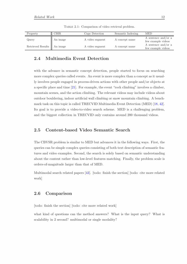
Table 2.1: Comparison of video retrieval problem.
Property CBIR Copy Detection Semantic Indexing MED
Query An image A video segment A concept nameA sentence and/or afew example videos
Retrieved Results An image A video segment A concept nameA sentence and/or afew example videos
2.4 Multimedia Event Detection
with the advance in semantic concept detection, people started to focus on searching
more complex queries called events. An event is more complex than a concept as it usual-
ly involves people engaged in process-driven actions with other people and/or objects at
a specific place and time [21]. For example, the event “rock climbing” involves a climber,
mountain scenes, and the action climbing. The relevant videos may include videos about
outdoor bouldering, indoor artificial wall climbing or snow mountain climbing. A bench-
mark task on this topic is called TRECVID Multimedia Event Detection (MED) [18, 42].
Its goal is to provide a video-to-video search scheme. MED is a challenging problem,
and the biggest collection in TRECVID only contains around 200 thousand videos.
2.5 Content-based Video Semantic Search
The CBVSR problem is similar to MED but advances it in the following ways. First, the
queries can be simple complex queries consisting of both text description of semantic fea-
tures and video examples. Second, the search is solely based on semantic understanding
about the content rather than low-level features matching. Finally, the problem scale is
orders-of-magnitude larger than that of MED.
Multimodal search related papers [43]. [todo: finish the section] [todo: cite more related
work]
2.6 Comparison
[todo: finish the section] [todo: cite more related work]
what kind of questions can the method answers? What is the input query? What is
scalability in 2 second? multimodal or single modality?

Chapter 3
Indexing Semantic Features
3.1 Introduction
Semantic indexing aims at extracting semantic features in the video content and in-
dexing them for efficient online search. In this chapter, we introduce the method for
extracting and indexing semantic features from the video content, focusing on adjusting
and indexing semantic concepts.
We consider indexing four types of semantic features in this thesis: visual concepts,
audio concepts ASR and OCR. ASR provides acoustic information about videos. It
especially benefits finding clues in close-to-camera and narrative videos such as “town
hall meeting” and “asking for directions”. OCR captures the text characters in videos
with low recall but high precision. The recognized characters are often not meaningful
words but sometimes can be a clue for fine-grained detection, e.g. distinguishing videos
about “baby shower” and “wedding shower”. ASR and OCR are text features, and thus
can be conveniently indexed by the standard inverted index. The automatically detected
text words in ASR and OCR in a video, after some preprocessing, can be treated as text
words in a document. The preprocessing includes creating a stop word list for ASR from
the English stop word list. The stop word lists for ASR includes utterances like “uh”,
“you know”, etc. For OCR, due to the noise in word detection, we need to remove the
words that do not exist in the English vocabulary.
How to index semantic concepts is an open question. Existing methods index a video by
the raw concept detection score that is dense and inconsistent [8, 14, 44–48]. This solu-
tion is mainly designed for analysis and search over a few thousand of videos, and cannot
scale to big data collections required for real world applications. Even though a modern
text retrieval system can already index and search over billions of text documents, the
13
Indexing Semantic Features 14
task is still very challenging for semantic video search. The main reason is that semantic
concepts are quite different from the text words, and semantic concept indexing is still
an understudied problem. Specifically, concepts are automatically extracted by detec-
tors with limited accuracy. The raw detection score associated with each concept is
inappropriate for indexing for two reasons. First, the distribution of the scores is dense,
i.e. a video contains every concept with a non-zero detection score, which is analogous
to a text document containing every word in the English vocabulary. The dense score
distribution hinders effective inverted indexing and search. Second, the raw score may
not capture the complex relations between concepts, e.g. a video may have a “puppy”
but not a “dog”. This type of inconsistency can lead to inaccurate search results.
To address this problem, we propose a novel step called concept adjustment that aims
at producing video (and video shot) representations that tend to be consistent with
the underlying concept representation. After adjustment, a video is represented by
a few salient and consistent concepts that can be efficiently indexed by the inverted
index. In theory, the proposed adjustment model is a general optimization framework
that incorporates existing techniques as special cases. In practice, as demonstrated
in our experiments, the adjustment increases the consistency with the ground-truth
concept representation on the real world TRECVID dataset. Unlike text words, semantic
concepts are associated with scores that indicate how confidently they are detected. We
propose an extended inverted index structure that incorporates the real-valued detection
scores and supports complex queries with Boolean and temporal operators.
Compared to existing methods, the proposed method exhibits the following three ben-
efits. First, it advances the text retrieval method for video retrieval. Therefore, while
existing methods fail as the size of the data grows, our method is scalable, extending the
current capability of semantic search by a few orders of magnitude while maintaining
state-of-the-art performance. Our experiments validate this argument. Second, we pro-
pose a novel component called concept adjustment in a common optimization framework
with solid probabilistic interpretations. Finally, our empirical studies shed some light on
the tradeoff between efficiency and accuracy in a large-scale video search system. These
observations will be helpful in guiding the design of future systems on related tasks.
The experimental results are promising on three datasets. On the TRECVIDMultimedia
Event Detection (MED), our method achieves comparable performance to state-of-the-
art systems, while reducing its index by a relative 97%. The results on the TRECVID
Semantic Indexing dataset demonstrate that the proposed adjustment model is able to
generate more accurate concept representation than baseline methods. The results on
the largest public multimedia dataset called YCCC100M [49] show that the method
is capable of indexing and searching over a large-scale video collection of 100 million
Indexing Semantic Features 15
Internet videos. It only takes 0.2 seconds on a single CPU core to search a collection
of 100 million Internet videos. Notably, the proposed method with reranking is able
to achieve by far the best result on the TRECVID MED 0Ex task, one of the most
representative and challenging tasks for semantic search in video.
3.2 Related Work
With the advance in object and action detection, people started to focus on searching
more complex queries called events. An event is more complex than a concept as it
usually involves people engaged in process-driven actions with other people and/or ob-
jects at a specific place and time [21]. For example, the event “rock climbing” involves
video clips such as outdoor bouldering, indoor artificial wall climbing or snow moun-
tain climbing. A benchmark task on this topic is called TRECVID Multimedia Event
Detection (MED). Its goal is to detect the occurrence of a main event occurring in a
video clip without any user-generated metadata. MED is divided into two scenarios
in terms of whether example videos are provided. When example videos are given, a
state-of-the-art system first train classifiers using multiple features and fuse the decision
of the individual classification results [50–58].
This thesis focuses on the other scenario named zero-example search (0Ex) where no
example videos are given. 0Ex mostly resembles a real world scenario, in which users
start the search without any example. As opposed to training an event detector, 0Ex
searches semantic concepts that are expected to occur in the relevant videos, e.g. we
might look for concepts like “car”, “bicycle”, “hand” and “tire” for the event “changing
a vehicle tire”. A few studies have been proposed on this topic [14, 44–48]. A closely
related work is detailed in [59], where the authors presented their lessons and observa-
tions in building a state-of-the-art semantic search engine for Internet videos. Existing
solutions are promising but only for a few thousand videos because they cannot scale
to big data collections. Therefore, the biggest collection in existing studies contains no
more than 200 thousand videos [4, 59].
Deng et al. [60] recently introduced label relation graphs called Hierarchy and Exclusion
(HEX) graphs. The idea is to infer a representation that maximizes the likelihood and
do not violate the label relation defined in the HEX graph.

Indexing Semantic Features 26
3.6 Experiments
3.6.1 Setups
Dataset and evaluation: The experiments are conducted on two TRECVID bench-
marks called Multimedia Event Detection (MED): MED13Test and MED14Test [4]. The
performance is evaluated by several metrics for a better understanding, which include:
P@20, Mean Reciprocal Rank (MRR), Mean Average Precision (MAP), and MAP@20,
where the MAP is the official metric used by NIST. Each set includes 20 events over
25,000 test videos. The official NIST’s test split is used. We also evaluate each experi-
ment on 10 randomly generated splits to reduce the split partition bias. All experiments
are conducted without using any example or text metedata.
Features and queries: Videos are indexed by semantic features including semantic
visual concepts, ASR, and OCR. For semantic concepts, 1,000 ImageNet concepts are
trained by the deep convolution neural networks [61]. The remaining 3,000+ concepts are
directly trained on videos by the self-paced learning pipeline [70, 71] on around 2 million
videos using improved dense trajectories [16]. The video datasets include Sports [72],
Yahoo Flickr Creative Common (YFCC100M) [49], Internet Archive Creative Common
(IACC) [4] and Do It Yourself (DIY) [73]. The details of these datasets can be found in
Table 3.1. The ASR module is built on EESEN and Kaldi [19, 20, 74]. OCR is extracted
by a commercial toolkit. Three sets of queries are used: 1) Expert queries are obtained
by human experts; 2) Auto queries are automatically generated by the Semantic Query
Generation (SQG) methods in [59] using ASR, OCR and visual concepts; 3) AutoVisual
queries are also automatically generated but only includes the visual concepts. The
Expert queries are used by default.
Configurations: The concept relation released by NIST is used to build the HEX
graph for IACC features [33]1. The adjustment is conducted at the video-level average
(p = 1 in Eq. (3.1)) so no shot-level exclusion relations are used. For other concept
features, since there is no public concept relation specification, we manually create the
HEX graph. The HEX graphs are empty for Sports and ImageNet features as there is
no evident hierarchical and exclusion relation in their concepts. We cluster the concepts
based on the correlation of their training labels, and include concepts that frequently
co-occur together into a group. The parameters are tuned on a validation sets, and
then are fixed across all experiment datasets including MED13Test, MED14Test and
YFCC100M. Specifically, the default parameters in Eq. (3.1) are p = 1, α = 0.95. β is
set as the top k detection scores in a video, and is different for each type of features: 60
1http://www-nlpir.nist.gov/projects/tv2012/tv11.sin.relations.txt
Indexing Semantic Features 27
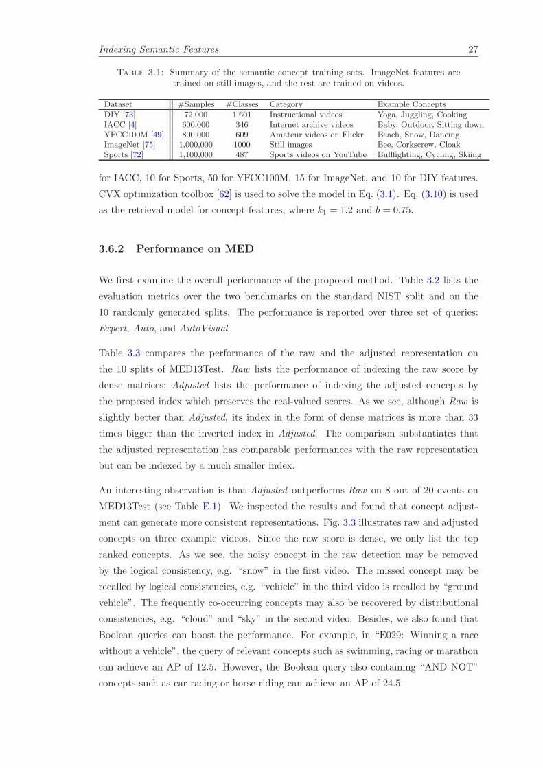
Table 3.1: Summary of the semantic concept training sets. ImageNet features aretrained on still images, and the rest are trained on videos.
Dataset #Samples #Classes Category Example Concepts
DIY [73] 72,000 1,601 Instructional videos Yoga, Juggling, CookingIACC [4] 600,000 346 Internet archive videos Baby, Outdoor, Sitting downYFCC100M [49] 800,000 609 Amateur videos on Flickr Beach, Snow, DancingImageNet [75] 1,000,000 1000 Still images Bee, Corkscrew, CloakSports [72] 1,100,000 487 Sports videos on YouTube Bullfighting, Cycling, Skiing
for IACC, 10 for Sports, 50 for YFCC100M, 15 for ImageNet, and 10 for DIY features.
CVX optimization toolbox [62] is used to solve the model in Eq. (3.1). Eq. (3.10) is used
as the retrieval model for concept features, where k1 = 1.2 and b = 0.75.
3.6.2 Performance on MED
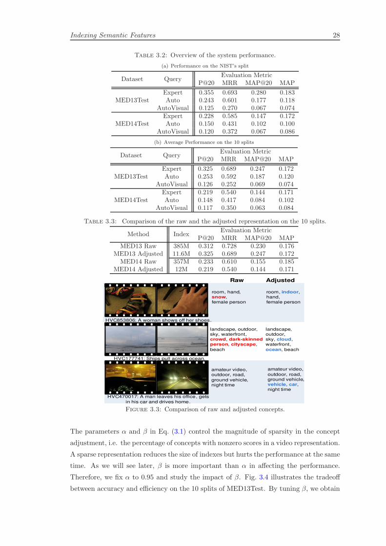
We first examine the overall performance of the proposed method. Table 3.2 lists the
evaluation metrics over the two benchmarks on the standard NIST split and on the
10 randomly generated splits. The performance is reported over three set of queries:
Expert, Auto, and AutoVisual.
Table 3.3 compares the performance of the raw and the adjusted representation on
the 10 splits of MED13Test. Raw lists the performance of indexing the raw score by
dense matrices; Adjusted lists the performance of indexing the adjusted concepts by
the proposed index which preserves the real-valued scores. As we see, although Raw is
slightly better than Adjusted, its index in the form of dense matrices is more than 33
times bigger than the inverted index in Adjusted. The comparison substantiates that
the adjusted representation has comparable performances with the raw representation
but can be indexed by a much smaller index.
An interesting observation is that Adjusted outperforms Raw on 8 out of 20 events on
MED13Test (see Table E.1). We inspected the results and found that concept adjust-
ment can generate more consistent representations. Fig. 3.3 illustrates raw and adjusted
concepts on three example videos. Since the raw score is dense, we only list the top
ranked concepts. As we see, the noisy concept in the raw detection may be removed
by the logical consistency, e.g. “snow” in the first video. The missed concept may be
recalled by logical consistencies, e.g. “vehicle” in the third video is recalled by “ground
vehicle”. The frequently co-occurring concepts may also be recovered by distributional
consistencies, e.g. “cloud” and “sky” in the second video. Besides, we also found that
Boolean queries can boost the performance. For example, in “E029: Winning a race
without a vehicle”, the query of relevant concepts such as swimming, racing or marathon
can achieve an AP of 12.5. However, the Boolean query also containing “AND NOT”
concepts such as car racing or horse riding can achieve an AP of 24.5.
Indexing Semantic Features 28
Table 3.2: Overview of the system performance.
(a) Performance on the NIST’s split
Dataset QueryEvaluation Metric
P@20 MRR MAP@20 MAP
MED13TestExpert 0.355 0.693 0.280 0.183Auto 0.243 0.601 0.177 0.118
AutoVisual 0.125 0.270 0.067 0.074
MED14TestExpert 0.228 0.585 0.147 0.172Auto 0.150 0.431 0.102 0.100
AutoVisual 0.120 0.372 0.067 0.086
(b) Average Performance on the 10 splits
Dataset QueryEvaluation Metric
P@20 MRR MAP@20 MAP
MED13TestExpert 0.325 0.689 0.247 0.172Auto 0.253 0.592 0.187 0.120
AutoVisual 0.126 0.252 0.069 0.074
MED14TestExpert 0.219 0.540 0.144 0.171Auto 0.148 0.417 0.084 0.102
AutoVisual 0.117 0.350 0.063 0.084
Table 3.3: Comparison of the raw and the adjusted representation on the 10 splits.
Method IndexEvaluation Metric
P@20 MRR MAP@20 MAPMED13 Raw 385M 0.312 0.728 0.230 0.176
MED13 Adjusted 11.6M 0.325 0.689 0.247 0.172MED14 Raw 357M 0.233 0.610 0.155 0.185
MED14 Adjusted 12M 0.219 0.540 0.144 0.171
HVC470017: A man leaves his office, gets
in his car and drives home.
HVC177741: Ships pull across ocean.
HVC853806: A woman shows off her shoes.
Raw Adjusted
amateur video,outdoor, road,
ground vehicle, night time
amateur video,
outdoor, road,ground vehicle,vehicle, car,night time
room, hand, snow, female person
room, indoor,hand, female person
landscape, outdoor, sky, waterfront, crowd, dark-skinnedperson, cityscape,
beach
landscape, outdoor, sky, cloud,waterfront,
ocean, beach
Figure 3.3: Comparison of raw and adjusted concepts.
The parameters α and β in Eq. (3.1) control the magnitude of sparsity in the concept
adjustment, i.e. the percentage of concepts with nonzero scores in a video representation.
A sparse representation reduces the size of indexes but hurts the performance at the same
time. As we will see later, β is more important than α in affecting the performance.
Therefore, we fix α to 0.95 and study the impact of β. Fig. 3.4 illustrates the tradeoff
between accuracy and efficiency on the 10 splits of MED13Test. By tuning β, we obtain

Indexing Semantic Features 29
different percentages of nonzero concepts in a video representation. The x-axis lists the
percentage in the log scale. x = 0 indicates the performance of ASR and OCR without
semantic concept features. We discovered that we do not need many concepts to index
a video, and a few adjusted concepts already preserve significant amount of information
for search. As we see, the best tradeoff in this problem is 4% of the total concepts
(i.e. 163 concepts). Further increasing the number of concepts only leads to marginal
performance gain.
16% 100%2% 3% 4% 8%1%0.4%0
0.1
0.2
0.3
0.4
0.5
0.6
0.7
Sparsity (percentage of concepts in the video)
P@20
MRR
MAP@20
MAP
Figure 3.4: The impact of parameter β. x = 0 indicates the performance of ASR andOCR without semantic concepts.
3.6.3 Comparison to State-of-the-art on MED
We then compare our best result with the published results on MED13Test. The exper-
iments are all conducted on the NIST’s split, and thus are comparable to each other. As
we see in Table 3.4, the proposed method has a comparable performance to the state-
of-the-art methods. Notably, the proposed method with one iteration of reranking [14]
is able to achieve the best result. The comparison substantiates that our method main-
tains state-of-the-art accuracy. It is worth emphasizing that the baseline methods may
not scale to big data sets, as the dense matrices are used to index all raw detection
scores [14, 47, 59].
Table 3.4: MAP (× 100) comparison with the published results on MED13Test.
Method Year MAP
Composite Concepts [45] 2014 6.4Tag Propagation [46] 2014 9.6MMPRF [44] 2014 10.1Clauses [48] 2014 11.2Multi-modal Fusion [47] 2014 12.6SPaR [14] 2014 12.9E-Lamp FullSys [59] 2015 20.7
Our System 2015 18.3Our System + reranking 2015 20.8

Indexing Semantic Features 30
3.6.4 Comparison to Top-k Thresholding on MED
We compare our full adjustment model with its special case top-k thresholding on
MED14Test. Theorem 3.4 indicates that the top-k thresholding results are optimal
solutions of our model in special cases. The experiments are conducted using IACC
SIN346 concept features that have large HEX graphs. We select the features because
large HEX graphs help compare the difference between the two methods. Table 3.5 lists
the average performance across 20 queries. We set the parameter k (equivalently β) to
be 50, and 60. As the experiment only uses 346 concepts, the results are worse than our
full systems using 3000+ concepts.Table 3.5: Comparison of the full adjustment model with its special case Top-k
Thresholding on the 10 splits of MED14Test.
Method kEvaluation Metric
P@20 MRR MAP@20 MAPOur Model 50 0.0392 0.137 0.0151 0.0225
Top-k 50 0.0342 0.0986 0.0117 0.0218Our Model 60 0.0388 0.132 0.0158 0.0239
Top-k 60 0.0310 0.103 0.0113 0.0220
As we see, the full adjustment model improves the accuracy and outperforms Top-k
thresholding in terms of P@20, MRR and MAP@20. We inspected the results and
found that the full adjustment model can generate more consistent representations (See
Fig. 3.3). The results suggest that the full model outperforms the special model in this
problem.
3.6.5 Accuracy of Concept Adjustment
Generally the comparison in terms of retrieval performance depends on the query words.
A query-independent way to verify the accuracy of the adjusted concept representation
is by comparing it to the ground truth representation. To this end, we conduct ex-
periments on the TRECVID Semantic Indexing (SIN) IACC set, where the manually
labeled concepts are available for each shot in a video. We use our detectors to extract
the raw shot-level detection score, and then apply the adjustment methods to obtain
the adjusted representation. The performance is evaluated by Root Mean Squared Error
(RMSE) to the ground truth concepts for the 1,500 test shots in 961 videos.
We compare our adjustment method with the baseline methods in Table 3.6, where HEX
Graph indicates the logical consistent representation [60] on the raw detection scores (i.e.
β = 0), and Group Lasso denotes the representation yield by Eq. (3.1) when α = 0. We
tune the parameter in each baseline method and report its best performance. As the
ground truth label is binary, we let the adjusted scores be binary in all methods. As we

Indexing Semantic Features 31
see, the proposed method outperforms all baseline methods. We hypothesize the reason
is that our method is the only one that combines the distributional consistency and the
logical consistency.
We study the parameter sensitivity in the proposed model. Fig. 3.5 plots the RMSE
under different parameter settings. Physically, α interpolates the group-wise and within-
group sparsity, and β determines the number of concepts in a video. As we see, the
parameter β is more sensitive than α, and accordingly we fix the value of α in practice.
Note the parameter β is also an important parameter in the baseline methods including
thresholding and top-k thresholding.
Table 3.6: Comparison of the adjusted representation and baseline methods on theTRECVID SIN set. The metric is Root Mean Squared Error (RMSE).
Method RMSE
Raw Score 7.671HEX Graph Only 8.090Thresholding 1.349Top-k Thresholding 1.624Group Lasso 1.570
Our method 1.236
0.2 0.4 0.6 0.8
00.2
0.40.8
0
0.5
1
1.5
2
2.5
3
alpha
beta
RM
SE
(a) Thresholding
5 11 17 23
00.2
0.40.8
0
0.5
1
1.5
2
2.5
alpha
beta (top−k)
RM
SE
(b) Top-k thresholding
Figure 3.5: Sensitivity study on the parameter α and β in our model.
3.6.6 Performance on YFCC100M
We apply the proposed method on YFCC100M, the largest public multimedia collec-
tion that has ever been released [49]. It contains about 0.8 million Internet videos
(approximately 12 million key shots) on Flickr. For each video and video shot, we ex-
tract the improved dense trajectory, and detect 3,000+ concepts by the off-the-shelf
detectors in Table 3.1. We implement our inverted index based on Lucene [76], and
a similar configuration described in Section 3.6.1 is used except we set b = 0 in the

Indexing Semantic Features 32
BM25 model. All experiments are conducted without using any example or text mete-
data. It is worth emphasizing that as the dataset is very big. The offline video index-
ing process costs considerable amount of computational resources in Pittsburgh super-
computing center. To this end, we share this valuable benchmark with our community
http://www.cs.cmu.edu/~lujiang/0Ex/mm15.html.
To validate the efficiency and scalability, we duplicate the original videos and video shots,
and create an artificial set of 100 million videos. We compare the search performance
of the proposed method to a common approach in existing studies that indexes the
video by dense matrices [47, 59]. The experiments are conducted on a single core of
Intel Xeon 2.53GHz CPU with 64GB memory. The performance is evaluated in terms
of the memory consumption and the online search efficiency. Fig. 3.6(a) compares the
in-memory index as the data size grows, where the x-axis denotes the number of videos
in the log scale, and the y-axis measures the index in GB. As we see, the baseline method
fails when the data reaches 5 million due to lack of memory. In contrast, our method
is scalable and only needs 550MB memory to search 100 million videos. The size of
the total inverted index on disk is only 20GB. Fig. 3.6(b) compares the online search
speed. We create 5 queries, run each query 100 times, and report the mean runtime in
milliseconds. A similar pattern can be observed in Fig. 3.6 that our method is much
more efficient than the baseline method and only costs 191ms to process a query on a
single core. The above results verify scalability and efficiency of the proposed method.
1 10 1000.5 5050
10
20
30
40
50
60
Total number of videos (million)
Inde
x si
ze (G
B)
Baseline in−memory index
Our on−disk index
Our in−memory index
Fail
(a) Index (in GB)
1 10 1000.5 5050
500
1000
1500
Total number of videos (million)
Ave
rage
sea
rch
time
(ms)
Baseline search time
Our search time
Fail
(b) Search Time (in ms)
Figure 3.6: The scalability and efficiency test on 100 million videos. Baseline methodfails when the data reaches 5 million due to the lack of memory. Our method is scalable
to 100 million videos.
As a demonstration, we use our system to find relevant videos for commercials. The
search is on 800 thousand Internet videos. We download 30 commercials from the
Internet, and manually create 30 semantic queries only using semantic visual concepts.
See detailed results in Table E.3. The ads can be organized in 5 categories. As we see, the
performance is much higher than the performance on the MED dataset in Table 3.2. The
improvement is a result of the increased data volumes. Fig. 3.7 plots the top 5 retrieved
videos are semantically relevant to the products in the ads. The results suggest that our
method may be useful in enhancing the relevance of in-video ads.

Indexing Semantic Features 33
Table 3.7: Average performance for 30 commercials on the YFCC100M set.
Category #AdsEvaluation Metric
P@20 MRR MAP@20
Sports 7 0.88 1.00 0.94Auto 2 0.85 1.00 0.95Grocery 8 0.84 0.93 0.88Traveling 3 0.96 1.00 0.96Miscellaneous 10 0.65 0.85 0.74
Average 30 0.81 0.93 0.86
Product: bicycle clothing
and helmets Query: superbike racing
OR bmx OR bike
Product: football shoesQuery: running AND
football
Top 5 retrieved videos in the YFCC100M set
Product: vehicle tireQuery: car OR exiting a vehicle OR sports car
racing OR car wheel
Figure 3.7: Top 5 retrieved results for 3 example ads on the YFCC100M dataset.
3.7 Summary
This chapter proposed a scalable solution for large-scale semantic search in video. The
proposed method extends the current capability of semantic video search by a few orders
of magnitude while maintaining state-of-the-art retrieval performance. A key in our solu-
tion is a novel step called concept adjustment that aims at representing a video by a few
salient and consistent concepts which can be efficiently indexed by the modified inverted
index. We introduced a novel adjustment model that is based on a concise optimization
framework with solid interpretations. We also discussed a solution that leverages the
text-based inverted index for video retrieval. Experimental results validated the effi-
cacy and the efficiency of the proposed method on several datasets. Specifically, the
experimental results on the challenging TRECVID MED benchmarks validate the pro-
posed method is of state-of-the-art accuracy. The results on the largest multimedia set
YFCC100M set verify the scalability and efficiency over a large collection of 100 million
Internet videos.
Chapter 4
Semantic Search
4.1 Introduction
In this chapter, we study the multimodal search process for semantic queries. The
process is called semantic search, which is also known as zero-example search [4] or 0Ex
for short, as zero examples are provided in the query. Searching by semantic queries is
more consistent with human’s understanding and reasoning about the task, where an
relevant video is characterized by the presence/absence of certain concepts rather than
local points/trajectories in the example videos.
We will focus on two subproblems, namely semantic query generation and multimodal
search. The semantic query generation is to map the out-of-vocabulary concepts in the
user query to their most relevant alternatives in the system vocabulary. The multimodal
search component aims at retrieving a ranked list using the multimodal features. We
empirically study the methods in the subproblems and share our observations and lessons
in building such a state-of-the-art system. The lessons are valuable because of not only
the effort in designing and conducting numerous experiments but also the considerable
computational resource to make the experiments possible. We believe the shared lessons
may significantly save the time and computational cycles for others who are interested
in this problem.
4.2 Related Work
A representative content-based retrieval task, initiated by the TRECVID community,
is called Multimedia Event Detection (MED) [4]. The task is to detect the occurrence
of a main event in a video clip without any textual metadata. The events of interest
34
Semantic Search 35
are mostly daily activities ranging from “birthday party” to “changing a vehicle tire”.
The event detection with zero training examples (0Ex) resembles the task of semantic
search. 0Ex is an understudied problem, and only few studies have been proposed very
recently [10, 44–48, 59, 77]. Dalton et al. [77] discussed a query expansion approach for
concept and text retrieval. Habibian et al. [45] proposed to index videos by composite
concepts that are trained by combining the labeled data of individual concepts. Wu et
al. [47] introduced a multimodal fusion method for semantic concepts and text features.
Given a set of tagged videos, Mazloom et al. [46] discussed a retrieval approach to
propagate the tags to unlabeled videos for event detection. Singh et al. [78] studied
a concept construction method that utilizes pairs of automatically discovered concepts
and then prunes those concepts that are unlikely to be helpful for retrieval. Jiang et
al. [14, 44] studied pseudo relevance feedback approaches which manage to significantly
improve the original retrieval results. Existing related works inspire our system.
4.3 Semantic Search
4.3.1 Semantic Query Generation
Users can express a semantic query in a variety of forms, such as a few concept names, a
sentence or a structured description. The Semantic Query Generation (SQG) component
translates a user query into a multimodal system query, all words of which exist in
the system vocabulary. A system vocabulary is the union of the dictionaries of all
semantic features in the system. The system vocabulary, to some extend, determines
what can be detected and thus searched by a system. For ASR/OCR features, the system
vocabulary is usually large enough to cover most words in user queries. For semantic
visual/audio concepts, however, the vocabulary is usually limited, and addressing the
out-of-vocabulary issue is a major challenge for SQG. The mapping between the user
and system query is usually achieved with the aid of an ontology such as WordNet and
Wikipedia. For example, a user query “golden retriever” may be translated to its most
relevant alternative “large-sized dog”, as the original concept may not exist in the system
vocabulary.
For example, in the MED benchmark, NIST provides a user query in the form of an
event-kit description, which includes a name, definition, explication and visual/acoustic
evidences. Table 4.1 shows the user query (event kit description) for the event “E011
Making a sandwich”. Its corresponding system query (with manual inspection) after
SQG is shown in Table 4.2. As we see, SQG is indeed a challenging task as it involves
understanding of text descriptions written in natural language.

Semantic Search 36
Table 4.1: User query (event-kit description) for the event “Making a sandwich”.
Event name Making a sandwich
DefinitionConstructing an edible food item from ingredients, often includ-ing one or more slices of bread plus fillings
Explication
Sandwiches are generally made by placing food items on topof a piece of bread, roll or similar item, and placing anotherpiece of bread on top of the food items. Sandwiches with onlyone slice of bread are less common and are called ”open facesandwiches”. The food items inserted within the slices of breadare known as ”fillings” and often include sliced meat, vegetables(commonly used vegetables include lettuce, tomatoes, onions,bell peppers, bean sprouts, cucumbers, and olives), and slicedor grated cheese. Often, a liquid or semi-liquid ”condiment”or ”spread” such as oil, mayonnaise, mustard, and/or flavoredsauce, is drizzled onto the sandwich or spread with a knife onthe bread or top of the sandwich fillers. The sandwich or breadused in the sandwich may also be heated in some way by placingit in a toaster, oven, frying pan, countertop grilling machine,microwave or grill. Sandwiches are a popular meal to make athome and are available for purchase in many cafes, conveniencestores, and as part of the lunch menu at many restaurants.
Evidences
sceneindoors (kitchen or restaurant or cafeteria) or outdoors (a parkor backyard)
objects/peoplebread of various types; fillings (meat, cheese, vegetables), condi-ments, knives, plates, other utensils
activitiesslicing, toasting bread, spreading condiments on bread, placingfillings on bread, cutting or dishing up fillings
audionoises from equipment hitting the work surface; narration of orcommentary on the process; noises emanating from equipment(e.g. microwave or griddle)
Table 4.2: System query for the event “E011 Making a sandwich”.
Event ID Name Category Relevance
Visual
sin346 133 food man made thing, food very relevantsin346 183 kitchen structure building, room very relevant
yfcc609 505 cookinghuman activity, workingutensil tool
very relevant
sin346 261 room structure building, room relevant
sin346 28 bar pubstructure build-ing,commercial building
relevant
yfcc609 145 lunch food, meal relevantyfcc609 92 dinner food, meal relevant
ASR ASR long
sandwich, food, bread, fil-l, place, meat, vegetable,cheese, condiment, knife,plate, utensil, slice, toast,spread, cut, dish
- relevant
OCR OCR short sandwich - relevant
The first step in SQG is to parse negations in the user query in order to recognize
counter-examples. The recognized examples can be either discarded or associated with
a “NOT” operator in the system query. We found that adding counter examples using
the Boolean NOT operator tends to improve performance. For example, in the query
“Winning a race without a vehicle”, the query including only relevant concepts such
as swimming, racing or marathon can achieve an AP of 12.57. However, the query

Semantic Search 37
also containing “AND NOT” concepts such as car racing, horse riding or bicycling can
achieve an AP of 24.50.
Given an event-kit description, a user query can be represented the event name (1-3
words) or the frequent words in the event-kit description (after removing the template
and stop words). This user query can be directly used as the system query for ASR/OCR
features as their vocabularies are sufficiently large. For visual/audio concepts, the query
are used to map the out-of-vocabulary words to their most relevant concepts in the
system vocabulary. To this end, we study the following classical mapping algorithms to
map a word in the user query to the concept in the system vocabulary:
Exact word matching: A straightforward mapping is matching the exact query word
(usually after stemming) against the concept name or the concept description. Generally,
for unambiguous words, this method has high precision but low recall.
WordNet mapping: This mapping calculates the similarity between two words in
terms of their distance in the WordNet taxonomy. The distance can be defined in
various ways such as structural depths in the hierarchy [79] or shared overlaps between
synonymous words [80]. Among the distance metrics, we found the structural depths
yields more robust results [79]. WordNet mapping is good at capturing synonyms and
subsumption relations between two nouns.
PMI mapping: The mapping calculates the Point-wise Mutual Information (PMI) [81]
between two words. Suppose qi and qj are two words in a user query, we have:
PMI(qi; qj) = logP (qi, qj |Cont)
P (qi|Cont)P (qj |Cont), (4.1)
where P (qi|Cont), P (qj |Cont) represent the probability of observing qi and qj in the on-
tology Cont (e.g. a collection of Wikipedia articles), which is calculated by the fraction
of the document containing the word. P (qi, qj |Cont) is the probability of observing the
document in which qi and qj both occur. PMI mapping assumes that similar words tend
to co-occur more frequently, and is good at capturing frequently co-occurring concepts
(both nouns and verbs).
Word embedding mapping: This mapping learns a word embedding that helps pre-
dict the surrounding words in a sentence [82, 83]. The learned embedding, usually by
neural network models, is in a lower-dimensional continuous vector space. The cosine
coefficient between two words is often used to measure their distance. It is fast and also
able to capture the frequent co-occurred words in similar contexts.
We found that discriminating the mapping relevance in a query may increase the per-
formance. In other words, the calculated relevance can be used to weight query terms.
Semantic Search 38
For example, the relevance can be categorized into discrete levels according to their
relevance to the user query. Table 4.2 have three levels of relevance: “very relevant”,
“relevant” and “slightly relevant”, and the levels are assigned to weight of 2.0, 1.0 and
0.5, respectively. We manually modified the relevance produced by the above automat-
ical mapping algorithms. In this way, we can observe an absolute 1-2% improvement
over the same query with no weights.
4.3.2 Retrieval Models
Given a system query, the multimodal search component aims at retrieving a ranked list
for each modality. We are interested in leveraging the well-studied text retrieval models
for video retrieval. This strategy allows us to utilize the infrastructure built for text
retrieval. There is no single retrieval model that can work the best for all modalities. As
a result, our system incorporates several classical retrieval models and applies them to
their most appropriate modalities. Let Q = q1, . . . , qn denote a system query. A retrieval
model ranks videos by the score s(d|Q), where d is a video in the video collection C. We
study the following retrieval models:
Vector Space Model (VSM): This model represents both a video and a query as
a vector of the words in the system vocabulary. The common vector representation
includes generic term frequency (tf) and term frequency-inverse document frequency
(tf-idf) [84]. s(d|Q) derives from either the dot product or the cosine coefficient between
the video and the query vector.
Okapi BM25: This model extends tf-idf representation by:
s(d|Q)=
n∑
i=1
log|C| − df(qi)+
12
df(qi)+12
tf(qi, d)(k1+1)
tf(qi, d)+k1(1−b+b len(d)len
), (4.2)
where |C| is the total number of videos in the collection. df(·) calculates the document
frequency for a given word in the collection; tf(qi, d) calculates the raw term frequency
for the word qi in the video d. Unlike text retrieval, in which document frequencies and
term frequencies are integers, in multimedia retrieval, these statistics can be real values
as concepts are associated with real-valued detection scores. len(d) calculates the sum
of concept or word detection scores in the video d, and len is the average video length
in the collection. k1 and b are two model parameters to tune [85]. In the experiments,
we set b = 0.75, and tune k1 in [1.2, 2.0].
Semantic Search 39
Language Model-JM Smoothing (LM-JM): The score is considered to be generated
by a unigram language model [86]:
s(d|Q) = log P (d|Q) ∝ log P (d) +n∑
i=1
log P (qi|d), (4.3)
where P (d) is usually assumed to be following the uniform distribution, i.e. the same
for every video, and can be dropped in the retrieval model. In some cases, we can
encode prior information about a video into P (d), such as its view count, length, and
viralness [87]. P (qi|d) is calculated from:
P (qi|d) = λtf(qi, d)∑w tf(w, d)
+ (1− λ)P (qi|C), (4.4)
where w enumerates all the words or the concepts in a given video. P (qi|C) is a smoother
that can be calculated by df(qi)/|C|. As we see, Eq. (4.4) linearly interpolates the
maximum likelihood estimation (first term) with the collection model (second term) by
a coefficient λ. The parameter is usually tuned in the range of [0.7, 0.9]. This model is
good for retrieving long text queries, e.g. the frequent words in the event kit description.
Language Model-Dirichlet Smoothing (LM-DL): This model adds a conjugate
prior (Dirichlet distribution) to the language model:
P (qi|d) =tf(qi, d) + µP (qi|C)∑
w tf(w, d) + µ, (4.5)
where µ is a coefficient balancing the likelihood model and the conjugate prior. It is
usually tuned in [0, 2000] [86]. This model is good for short text queries, e.g. the event
name.
4.4 Experiments
4.4.1 Setups
Dataset and evaluation: The experiments are conducted on two TRECVID bench-
marks called Multimedia Event Detection (MED): MED13Test and MED14Test [4]. The
performance is evaluated by the official metric Mean Average Precision (MAP). Each
set includes 20 events over 25,000 test videos. The official NIST’s test split is used.
We also evaluate each experiment on 10 randomly generated splits to reduce the bias
brought by the split partition. The mean and 90% confidence interval are reported. All
experiments are conducted without using any example or text metedata.

Semantic Search 40
Features and queries: Videos are indexed by semantic features including semantic
visual concepts, ASR, and OCR. The same semantic features described in Section 3.6.1
are used in the experiments, except here the features are represented by the raw detection
scores before the adjustment. See the details of concept features in Table 3.1. we share
our features and experimental results on the benchmark
http://www.cs.cmu.edu/~lujiang/0Ex/icmr15.html.
The user query is the event-kit description. For ASR/OCR, the automatically generated
event name and description representations are directly used as the system query. The
system query for semantic concepts is obtained by a two-step procedure: a preliminary
mapping is automatically generated by the discussed mapping algorithms. The results
are then examined by human experts to figure out the final system query. We call these
queries Expert queries. Besides, we also study the queries automatically generated by
the mapping algorithm called “Auto SQG” in Section 4.4.2.
Configurations: In the multimodal search component, by default, the LM-JM model
(λ = 0.7) is used for ASR/OCR for the frequent-words in the event-kit description.
BM25 is used for ASR [88] and OCR features for the event name query (1-3 words),
where k1 = 1.2 and b = 0.75. Both the frequent-words query and the event name query
are automatically generated without manual inspection. While parsing the frequent
words in the event-kit description, the stop and template words are first removed, and
words in the evidence section are counted three times. After parsing, the words with
the frequency ≥ 3 are then used in the query. VSM-tf model is applied to all semantic
concept features.
In the SQG component, the exact word matching algorithm finds the concept name in
the frequent event-kit words (frequency ≥ 3). The WordNet mapping uses the distance
metrics in [79] as the default metric. We build an inverted index over the Wikipedia
corpus (about 6 million articles), and use it to calculate the PMI mapping. To calculate
the statistics, we online issue queries to the index. A pre-trained word embedding trained
on Wikipedia [83] is used to calculated the word embedding mapping.
4.4.2 Semantic Matching in SQG
We apply the SQG mapping algorithms in Section 4.3.1 to map the user query to the
concepts in the vocabulary. The experiments are conducted only using semantic concept
features. We use two metrics to compare these mapping algorithms. One is the precision
of the 5 most relevant concepts returned by each algorithm. We manually assess the rel-
evance for 10 events (E031-E040) on 4 concept features (i.e. 200 pairs for each mapping
algorithm). The other is the MAP obtained by the 3 most relevant concepts. Table 4.3

Semantic Search 41
lists the results, where the last column lists the runtime of calculating the mapping
between 1,000 pairs of words. The second last row (Fusion) indicates the average fusion
of the results of all mapping algorithms. As we see, in terms of P@5, PMI is slightly
better than others, but it is also the slowest because its calculation involves looking up
a index of 6 million text documents in Wikipedia. Fusion of all mapping results yields
a better P@5.
We then combine the automatically mapped semantic concepts with the automatically
generated ASR and OCR query. Here we assume users have specified which feature to
use for each query, and SQG is used to automatically find relevant concepts or words
in the specified features. We obtain this information in the event-kit description. For
example, we will use ASR when we find words “narration/narrating” and “process” in
the event-kit description. An event that has these words in the description tends to
be an instructional event, such as “Making a sandwich” and “Repairing an appliance”,
in which the spoken words are more likely to be detected accurately. Our result can
be understood as an overestimate of a fully-automatic SQG system, in which users do
not even need to specify the feature. As we see in Table 4.3, PMI performs the best
on MED13Test whereas on MED14Test it is Exact Word Matching. The fusion of all
mapping results (the second last row) improves the MAP on both the datasets. We then
fine-tune the parameters of the mapping fusion and build our AutoSQG system (the last
row).
As we see, AutoSQG only achieves about 55% of the full system’s MAP. Several reasons
account for the performance drop: 1) the concept name does not accurately describe
what is being detected; 2) the quality of mapping is limited (P@5=0.42); 3) relevant con-
cepts are not necessarily discriminative concepts. For example, “animal” and “throwing
ball” appear to be relevant to the query “playing a fetch”, but the former is too general
and the latter is about throwing a baseball which is visually different; “dog” is much
less discriminative than “group of dogs” for the query “dog show”. The results suggest
that the automatic SQG is not well-understood. The proposed automatic mappings are
still very preliminary, and could be further refined by manual inspection. A significant
drawback of current mapping algorithms is representing a concept as a few words. How-
ever, in our manual assessment, we regard a concept as a multimodal document that
includes a name, description, category, reliability (accuracy) and examples of the top
detected video snippet.
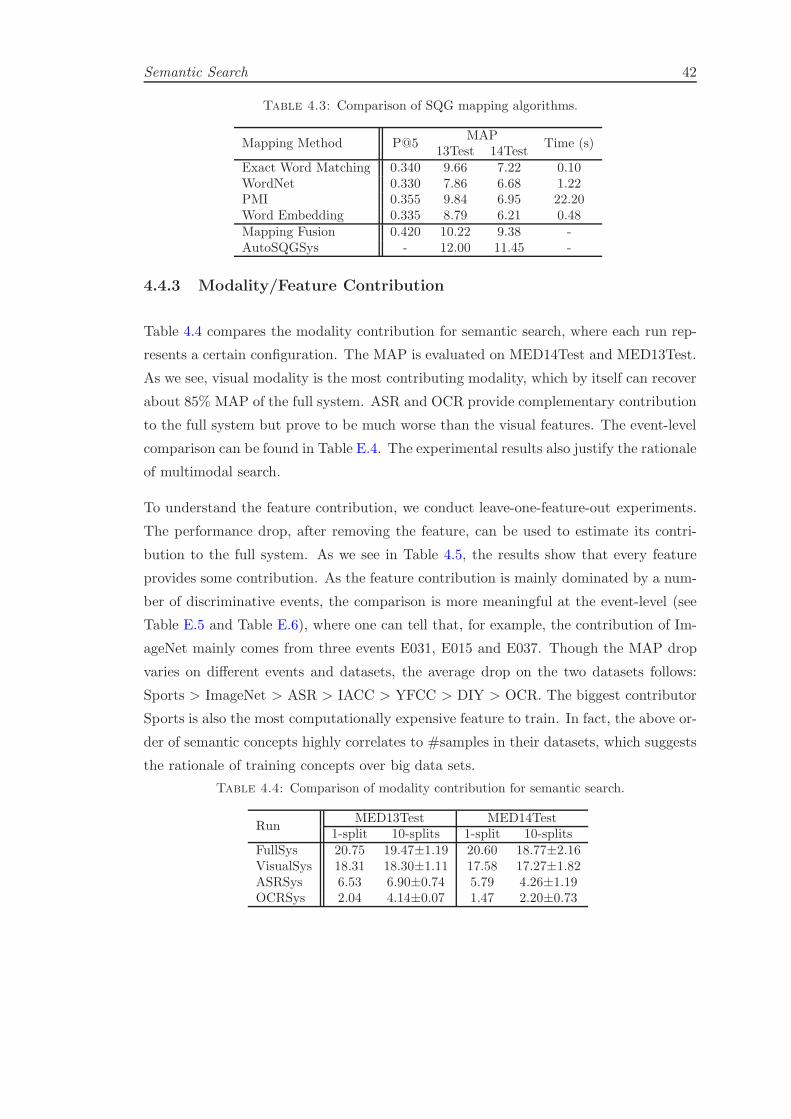
Semantic Search 42
Table 4.3: Comparison of SQG mapping algorithms.
Mapping Method P@5MAP
Time (s)13Test 14Test
Exact Word Matching 0.340 9.66 7.22 0.10WordNet 0.330 7.86 6.68 1.22PMI 0.355 9.84 6.95 22.20Word Embedding 0.335 8.79 6.21 0.48Mapping Fusion 0.420 10.22 9.38 -AutoSQGSys - 12.00 11.45 -
4.4.3 Modality/Feature Contribution
Table 4.4 compares the modality contribution for semantic search, where each run rep-
resents a certain configuration. The MAP is evaluated on MED14Test and MED13Test.
As we see, visual modality is the most contributing modality, which by itself can recover
about 85% MAP of the full system. ASR and OCR provide complementary contribution
to the full system but prove to be much worse than the visual features. The event-level
comparison can be found in Table E.4. The experimental results also justify the rationale
of multimodal search.
To understand the feature contribution, we conduct leave-one-feature-out experiments.
The performance drop, after removing the feature, can be used to estimate its contri-
bution to the full system. As we see in Table 4.5, the results show that every feature
provides some contribution. As the feature contribution is mainly dominated by a num-
ber of discriminative events, the comparison is more meaningful at the event-level (see
Table E.5 and Table E.6), where one can tell that, for example, the contribution of Im-
ageNet mainly comes from three events E031, E015 and E037. Though the MAP drop
varies on different events and datasets, the average drop on the two datasets follows:
Sports > ImageNet > ASR > IACC > YFCC > DIY > OCR. The biggest contributor
Sports is also the most computationally expensive feature to train. In fact, the above or-
der of semantic concepts highly correlates to #samples in their datasets, which suggests
the rationale of training concepts over big data sets.
Table 4.4: Comparison of modality contribution for semantic search.
RunMED13Test MED14Test
1-split 10-splits 1-split 10-splitsFullSys 20.75 19.47±1.19 20.60 18.77±2.16VisualSys 18.31 18.30±1.11 17.58 17.27±1.82ASRSys 6.53 6.90±0.74 5.79 4.26±1.19OCRSys 2.04 4.14±0.07 1.47 2.20±0.73
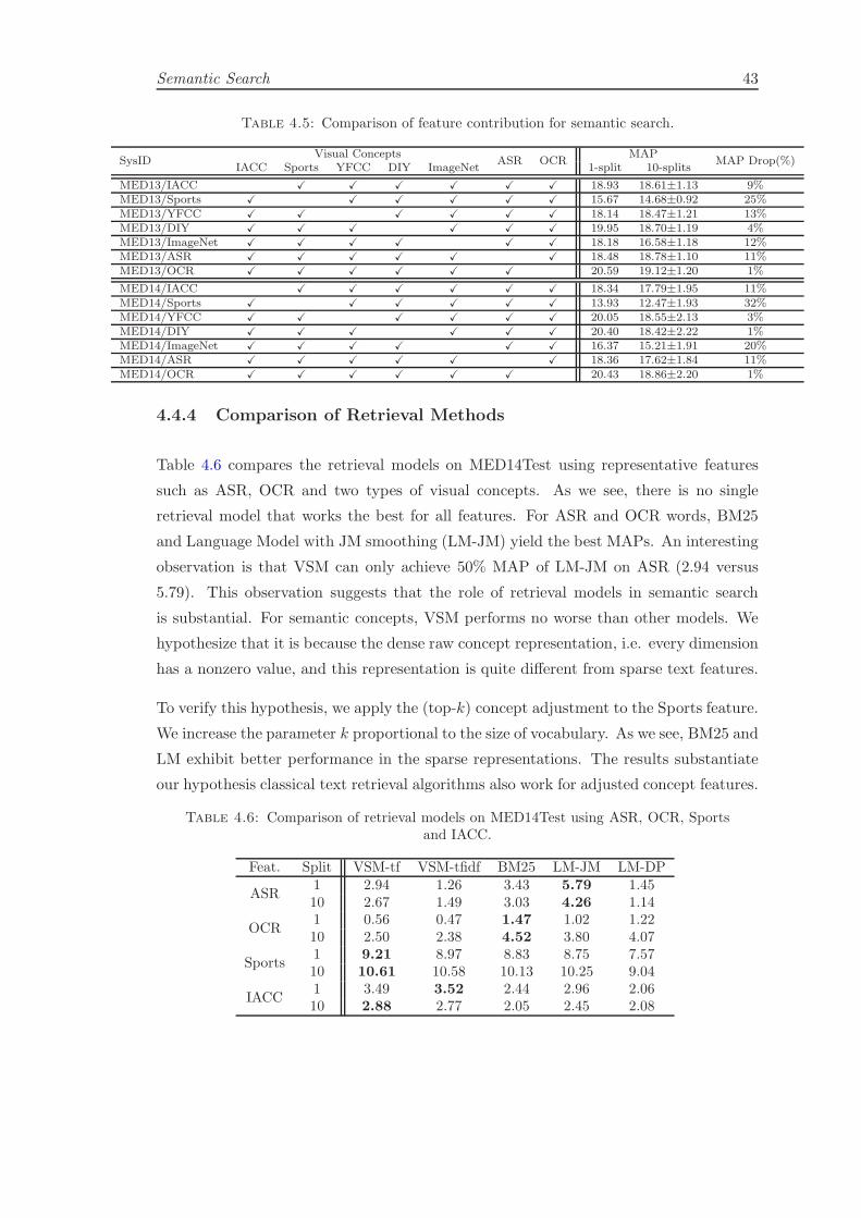
Semantic Search 43
Table 4.5: Comparison of feature contribution for semantic search.
SysIDVisual Concepts
ASR OCRMAP
MAP Drop(%)IACC Sports YFCC DIY ImageNet 1-split 10-splits
MED13/IACC X X X X X X 18.93 18.61±1.13 9%MED13/Sports X X X X X X 15.67 14.68±0.92 25%MED13/YFCC X X X X X X 18.14 18.47±1.21 13%MED13/DIY X X X X X X 19.95 18.70±1.19 4%MED13/ImageNet X X X X X X 18.18 16.58±1.18 12%MED13/ASR X X X X X X 18.48 18.78±1.10 11%MED13/OCR X X X X X X 20.59 19.12±1.20 1%
MED14/IACC X X X X X X 18.34 17.79±1.95 11%MED14/Sports X X X X X X 13.93 12.47±1.93 32%MED14/YFCC X X X X X X 20.05 18.55±2.13 3%MED14/DIY X X X X X X 20.40 18.42±2.22 1%MED14/ImageNet X X X X X X 16.37 15.21±1.91 20%MED14/ASR X X X X X X 18.36 17.62±1.84 11%MED14/OCR X X X X X X 20.43 18.86±2.20 1%
4.4.4 Comparison of Retrieval Methods
Table 4.6 compares the retrieval models on MED14Test using representative features
such as ASR, OCR and two types of visual concepts. As we see, there is no single
retrieval model that works the best for all features. For ASR and OCR words, BM25
and Language Model with JM smoothing (LM-JM) yield the best MAPs. An interesting
observation is that VSM can only achieve 50% MAP of LM-JM on ASR (2.94 versus
5.79). This observation suggests that the role of retrieval models in semantic search
is substantial. For semantic concepts, VSM performs no worse than other models. We
hypothesize that it is because the dense raw concept representation, i.e. every dimension
has a nonzero value, and this representation is quite different from sparse text features.
To verify this hypothesis, we apply the (top-k) concept adjustment to the Sports feature.
We increase the parameter k proportional to the size of vocabulary. As we see, BM25 and
LM exhibit better performance in the sparse representations. The results substantiate
our hypothesis classical text retrieval algorithms also work for adjusted concept features.
Table 4.6: Comparison of retrieval models on MED14Test using ASR, OCR, Sportsand IACC.
Feat. Split VSM-tf VSM-tfidf BM25 LM-JM LM-DP
ASR1 2.94 1.26 3.43 5.79 1.4510 2.67 1.49 3.03 4.26 1.14
OCR1 0.56 0.47 1.47 1.02 1.2210 2.50 2.38 4.52 3.80 4.07
Sports1 9.21 8.97 8.83 8.75 7.5710 10.61 10.58 10.13 10.25 9.04
IACC1 3.49 3.52 2.44 2.96 2.0610 2.88 2.77 2.05 2.45 2.08
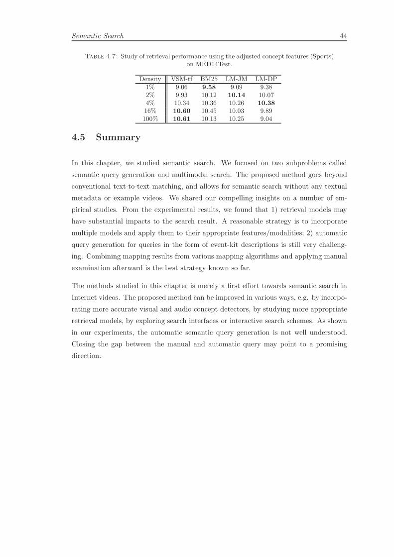
Semantic Search 44
Table 4.7: Study of retrieval performance using the adjusted concept features (Sports)on MED14Test.
Density VSM-tf BM25 LM-JM LM-DP1% 9.06 9.58 9.09 9.382% 9.93 10.12 10.14 10.074% 10.34 10.36 10.26 10.3816% 10.60 10.45 10.03 9.89100% 10.61 10.13 10.25 9.04
4.5 Summary
In this chapter, we studied semantic search. We focused on two subproblems called
semantic query generation and multimodal search. The proposed method goes beyond
conventional text-to-text matching, and allows for semantic search without any textual
metadata or example videos. We shared our compelling insights on a number of em-
pirical studies. From the experimental results, we found that 1) retrieval models may
have substantial impacts to the search result. A reasonable strategy is to incorporate
multiple models and apply them to their appropriate features/modalities; 2) automatic
query generation for queries in the form of event-kit descriptions is still very challeng-
ing. Combining mapping results from various mapping algorithms and applying manual
examination afterward is the best strategy known so far.
The methods studied in this chapter is merely a first effort towards semantic search in
Internet videos. The proposed method can be improved in various ways, e.g. by incorpo-
rating more accurate visual and audio concept detectors, by studying more appropriate
retrieval models, by exploring search interfaces or interactive search schemes. As shown
in our experiments, the automatic semantic query generation is not well understood.
Closing the gap between the manual and automatic query may point to a promising
direction.

Chapter 5
Hybrid Search
Propose a new methods for
5.1 Introduction
5.2 Related Work
5.3 Scalable Few Example Search
5.4 Experiments
45
Chapter 6
Video Reranking
6.1 Introduction
Reranking is a technique to improve the quality of search results [89]. The intuition is
that the initial ranked result brought by the query has noise which can be refined by
the multimodal information residing in the retrieved documents, images or videos. For
example, in image search, the reranking is performed based on the results of text-to-
text search, in which the initial results are retrieved by matching images’ surrounding
texts [90]. Studies show that reranking can usually yield improvement of the initial
retrieved result [91, 92]. Reranking by multimodal content-based search is still an un-
derstudied problem. It is more challenging than reranking by text-to-text search in
image search, since the content features not only come from multiple modalities but also
are much more noisy. In this chapter, we will introduce two content-based reranking
methods, and discuss how they can be united in the same algorithm.
In a generic reranking method, we would first select a few videos, and assign assumed
labels to them. Since no ground-truth label is used, the assumed labels are called “pseu-
do labels”. The samples with pseudo labels are used to build a reranking model. The
statistics collected from the model is used to improve the initial ranked list. Most exist-
ing reranking or Pseudo-Relevance Feedback (PRF) methods are designed to construct
pseudo labels from a single ranked list, e.g. from the text search [24, 93, 94] or the
visual image search [95, 96]. Due to the challenge of multimedia retrieval, features from
multiple modalities are usually used to achieve better performance [21, 56]. However,
performing multimodal reranking is an important yet unaddressed problem. The key
challenge is to jointly derive a pseudo label set from multiple ranked lists. Although
reranking may not be a novel idea, reranking by multimodal content-based search is
46

Video Reranking 47
Figure 6.1: Comparison of binary, predefined and learned weights on the query “Birth-day Party”. All videos are used as positive in reranking. Learned weights are learned
by the proposed method.
clearly understudied and worthy of exploration, as existing studies mainly concentrate
on text-to-text search.
Besides, an important step in this process is to assign weights to the samples with
pseudo labels. The main strategy in current reranking methods is to assign binary (or
predefined) weights to videos at different rank positions. These weighting schemes are
simple to implement, yet may lead to suboptimal solutions. For example, the reranking
methods in [44, 96, 97] assume that top-ranked videos are of equal importance (binary
weights). The fact is that, however, videos ranked higher are generally more accurate,
and thus more “important”, than those ranked lower. The predefined weights [94] may
be able to distinguish importance but they are derived independently of reranking mod-
els, and thus may not faithfully reflect the latent importance. For example, Fig. 6.1
illustrates a ranked list of videos about “birthday party”, where all videos will be used
as positive in reranking; the top two are true positive; the third video is a negative but
closely related video on wedding shower due to the common concepts such as “gift”,
“cake” and “cheering”; the fourth video is completely unrelated. As illustrated, neither
binary nor predefined weights reflects the latent importance residing in the videos. An-
other important drawback of binary or predefined weighting is that since the weights
are designed based on empirical experience, it is unclear where does, or even whether,
the process would converge.
An ideal reranking method would consider the multimodal features and assign appropri-
ate weights in a theoretically sound manner. To this end, we propose two content-based
reranking models. The first model is called MultiModal Pseudo Relevance Feedback
(MMPRF) which conducts the feedback jointly on multiple modalities leading to a con-
sistent joint reranking model. MMPRF utilizes the ranked lists of all modalities and
combines them in a principled approach. MMPRF is a first attempt that leverages both
Video Reranking 48
high-level and low-level features for semantic search in a CBVSR system. As we know,
it is impossible to use low-level features for semantic search, it is impossible to map the
text-like query to the low-level feature without any training data. MMPRF circumvents
the difficulty by transferring this problem into a supervised problem on pseudo labels.
The second model is called Self-Paced Reranking (SPaR) which assigns weights adap-
tively in a self-paced fashion. The method is established on the self-paced learning
theory [98, 99]. The theory is inspired by the learning process of humans and animals,
where samples are not presented randomly but organized in a meaningful order which
illustrates from easy to gradually more complex examples [98]. In the context of rerank-
ing problems, easy samples are the top-ranked videos that have smaller loss. As opposed
to utilizing all samples to learn a model simultaneously, the proposed model is learned
gradually from easy to more complex samples. As the name “self-paced” suggests, in ev-
ery iteration, SPaR examines the “easiness” of each sample based on what it has already
learned, and adaptively determines their weights to be used in the next iteration.
SPaR represents a general multimodal reranking method. MMPRF is a special case
of the proposed method that only uses the binary weighting. Compared with existing
reranking methods, SPaR has the following three benefits. First, it is established on a
solid theory, and of useful properties that can be theoretically verified. For example,
SPaR has a concise mathematical objective to optimize, and its convergence property
can be theoretically proved. Second, SPaR represents a general framework for reranking
on multimodal data, which includes other methods [44, 97, 100], such as MMPRF, as
special cases. The connection is useful because once an existing method is modeled
as a special case of SPaR, the optimization methods discussed in this chapter become
immediately applicable to analyze, and even solve the problem. Third, SPaR offers
a compelling insight into reranking by multimodal content-based search [44, 45, 101],
where the initial ranked lists are retrieved by content-based search.
The experimental results show promising results on several challenging datasets. As
for semantic search, on the MED dataset, MMPRF and SPaR significantly improve
the state-of-the-art baseline reranking methods with statistically significant differences;
SPaR also outperforms the state-of-the-art reranking methods on an image reranking
dataset called Web Query. For hybrid search, SPaR yields statistically significant im-
provements over the initial search results.
Video Reranking 49
6.2 Related Work
The pseudo labels are usually obtained from a single modality in the literature. On
the text modality, reranking, usually known as PRF, has been extensively studied. In
the vector space model, the Rocchio algorithm [24] is broadly used, where the original
query vector is modified by the vectors of relevant and irrelevant documents. Since a
document’s true relevance judgment is unavailable, the top-ranked and bottom-ranked
documents in the retrieved list are used to approximate the relevant and irrelevant
documents. In the language model, PRF is usually performed with a Relevance Model
(RM) [93, 102]. The idea is to estimate the probability of a word in the relevance model,
and feed the probability back to smooth the query likelihood in the language model.
Because the relevance model is unknown, RM assumes the top-ranked documents imply
the distribution of the unknown relevance model. Several extensions have been proposed
to improve RM. For example, instead of using the top-ranked documents, Lee et al.
proposed a cluster-based resampling method to select better feedback documents [103].
Cao et al. explored a supervised approach to select good expansion terms based on a
pre-trained classifier [104].
Reranking has also been shown to be effective in image and video retrieval. Yan et
al. proposed a classification-based PRF [95–97], where the query image and its most
dissimilar images are used as pseudo samples. The idea is to train an imbalanced SVM
classifier, biased towards negative pseudo samples, as true negatives are usually much
easier to find. In [94], the pseudo negatives, sampled from the ranked list of a text query,
are first grouped into several clusters and the clusters’ conditional probabilities are fed
back to alter the initial ranked list. Similar to [103], the role of clustering is to reduce the
noise in the initial text ranked list. In [100, 105], the authors incorporated pseudo labels
into the learning to rank paradigm. The idea is to learn a ranking function by optimizing
the pair-wise or list-wise orders between pseudo positive and negative samples. In [106],
the relevance judgments over the top-ranked videos are provided by users. Then an SVM
is trained using visual features represented in the Fisher vector. However, the manual
inspection of the search results is prohibited in many problems.
Existing reranking methods are mainly performed based on text-to-text search results,
i.e. the initial ranked list is retrieved by text/keyword matching [105, 107]. In terms of
the types of the reranking model, these methods can be categorized into Classification,
Clustering, Graph and LETOR (LEarning-TO-Rank) based reranking. In Classification-
based reranking [97], a classifier is trained upon the pseudo label set, and then tested on
retrieved videos to obtain a reranked list. Similarly, in LETOR-based reranking [108]
instead of a binary classifier, a ranking function is learned by the pair-wise [100] or
list-wise [91, 105] RankSVM. In Clustering-based reranking [94], the retrieved videos are

Video Reranking 50
aggregated into clusters, and the clusters’ conditional probabilities of the pseudo samples
are used to obtain a reranked list. The role of clustering is to reduce the noise in the
initial reranking. In Graph-based reranking [109, 110], the graph of retrieved samples
needs to be first constructed, on which the initial ranking scores are propagated by
methods such as the random walk [21], under the assumption that visually similar videos
usually have similar ranks. Generally, reranking methods, including the above methods,
are unsupervised methods. There also exist some studies on supervised reranking [90,
107]. Although reranking may not be a novel idea, reranking by multimodal content-
based search is clearly understudied and worthy of exploration. Only a few methods
have been proposed to conduct reranking based on content-based search results without
examples (or training data).
6.3 MMPRF
The intuition behind MMPRF is that the relevant videos can be modeled by a joint
discriminative model trained on all modalities. Suppose dj is a video in the collection,
the probability of it being relevant can be calculated from the posterior P (yj|dj ; Θ),
where yj is the (pseudo) label for jth video, and Θ denotes the parameter in the joint
model. In PRF methods on unimodal data, the partial model is trained on a single
modality [95, 96]. We model the ranked list of each modality by its partial model, and
our goal is to recover a joint model from these partial models. Formally, we use logistic
regression as the discriminative model. For ith modality, the probability of a video being
relevant can be calculated from
P (yj|dj ; Θi) =1
1 + exp−θTi wij, (6.1)
wherewij represents the video dj’s feature vector from the ith modality. Θi = θi denotes
the model parameter vector for the ith modality. For a clearer notation, the intercept
parameter b is absorbed into the vector θi. According to [95], the parameters Θi can be
independently estimated using the top ranked k+ samples and the bottom ranked k−
samples in the ith modality, where k+ and k− control the number of pseudo positive
and pseudo negative samples, respectively.
However, the models estimated independently on each modality can be inconsistent.
For example, a video may be used as a pseudo positive in one modality but as a pseudo
negative in another modality. An effective approach to find the consistent pseudo label
set is by Maximum Likelihood Estimation (MLE) with respect to the label set likelihood
over all modalities. Formally, let Ω denotes the union of feedback videos of all modalities.
Video Reranking 51
Our objective is to find a pseudo label set that maximizes:
argmaxy
m∑
i=1
lnL(y; Ω,Θi)
s.t. ||y||1 ≤ k+; y ∈ 0, 1|Ω|
(6.2)
where |Ω| represents the total number of unique pseudo samples, and y = [y1, ...y|Ω|]T
represents their pseudo labels. L(y; Ω,Θi) is the likelihood of the label set y in the ith
modality. The sum of likelihood in Eq. (6.2) indicates that each label in the pseudo
label set needs to be verified by all modalities and the desired label set satisfies the most
modalities. The selection process is analogous to voting, where every modality votes
using the likelihood and the better the labels fit a modality, the higher the likelihood
is, and vice versa. The set with the highest votes is selected as the pseudo label set.
Because each pseudo label is validated by all modalities, the false positives in a single
modality may be corrected during the voting. This property is unavailable when only a
single modality is considered.
To solve Eq. (6.2), we rewrite the logarithmic likelihood using Eq. (6.1)
lnL(y; Ω,Θi) = ln∏
dj∈ΩP (yj|dj ,Θi)
yj (1− P (yj|dj ,Θi))(1−yj )
=
|Ω|∑
j=1
yjθTi wij − θTi wij − ln(1 + exp−θTi wij)
(6.3)
As mentioned above, θi can be independently estimated using the top-ranked and
bottom-ranked samples in the ith modality. wij is the known feature vector. Plug-
ging Eq. (6.3) back to Eq. (6.2) and dropping the constants, the objective function in
Eq. (6.3) becomes
argmaxy
m∑
i=1
lnL(y; Ω,Θi) = argmaxy
m∑
i=1
|Ω|∑
j=1
yjθTi wij.
s.t. ||y||1 ≤ k+; y ∈ 0, 1|Ω|
(6.4)
As can be seen, the problem of finding the pseudo label set with the maximum likelihood
has been transferred to an integer programming problem, where the objective function
is the sum of logarithmic likelihood across all modalities and the pseudo labels are
restricted to be binary numbers.
The pseudo negative samples can be randomly sampled from the bottom-ranked sam-
ples, as suggested in [94, 95]. In the worst case, suppose n pseudo negative samples
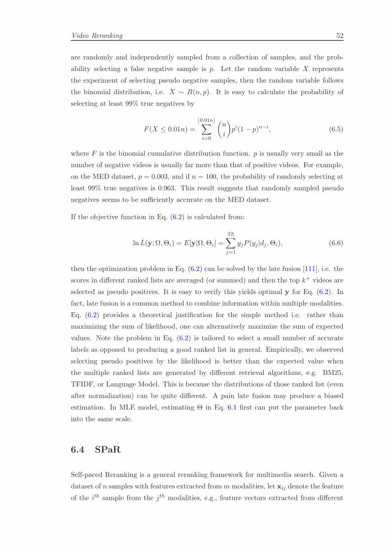
Video Reranking 52
are randomly and independently sampled from a collection of samples, and the prob-
ability selecting a false negative sample is p. Let the random variable X represents
the experiment of selecting pseudo negative samples, then the random variable follows
the binomial distribution, i.e. X ∼ B(n, p). It is easy to calculate the probability of
selecting at least 99% true negatives by
F (X ≤ 0.01n) =
⌊0.01n⌋∑
i=0
(n
i
)pi(1− p)n−i, (6.5)
where F is the binomial cumulative distribution function. p is usually very small as the
number of negative videos is usually far more than that of positive videos. For example,
on the MED dataset, p = 0.003, and if n = 100, the probability of randomly selecting at
least 99% true negatives is 0.963. This result suggests that randomly sampled pseudo
negatives seems to be sufficiently accurate on the MED dataset.
If the objective function in Eq. (6.2) is calculated from:
ln L(y; Ω,Θi) = E[y|Ω,Θi] =
|Ω|∑
j=1
yjP (yj|dj ,Θi), (6.6)
then the optimization problem in Eq. (6.2) can be solved by the late fusion [111], i.e. the
scores in different ranked lists are averaged (or summed) and then the top k+ videos are
selected as pseudo positives. It is easy to verify this yields optimal y for Eq. (6.2). In
fact, late fusion is a common method to combine information within multiple modalities.
Eq. (6.2) provides a theoretical justification for the simple method i.e. rather than
maximizing the sum of likelihood, one can alternatively maximize the sum of expected
values. Note the problem in Eq. (6.2) is tailored to select a small number of accurate
labels as opposed to producing a good ranked list in general. Empirically, we observed
selecting pseudo positives by the likelihood is better than the expected value when
the multiple ranked lists are generated by different retrieval algorithms, e.g. BM25,
TFIDF, or Language Model. This is because the distributions of those ranked list (even
after normalization) can be quite different. A pain late fusion may produce a biased
estimation. In MLE model, estimating Θ in Eq. 6.1 first can put the parameter back
into the same scale.
6.4 SPaR
Self-paced Reranking is a general reranking framework for multimedia search. Given a
dataset of n samples with features extracted frommmodalities, let xij denote the feature
of the ith sample from the jth modalities, e.g., feature vectors extracted from different

Video Reranking 53
channels of a video. yi ∈ −1, 1 represents the pseudo label for the ith sample whose
values are assumed as the true labels are unknown to reranking methods. The kernel
SVM is used to illustrate the algorithm due to its robustness and decent performance
in reranking [96]. We will discuss how to generalize it to other models in Section 6.4.3.
Let Θj = wj , bj denote the classifier parameters for the jth modality, which includes
a coefficient vector wj and a bias term bj . Let v = [v1, ..., vn]T denote the weighting
parameters for all samples. Inspired by the self-paced learning [99], suppose n is the
total number of samples; m is the total number of modalities; the objective function E
can be formulated as:
minΘ1,...,Θm,y,v
E(Θ1, ...,Θm,v,y;C, k) =m∑
j=1
minΘj ,y,v
E(Θj,v,y;C, k)
= miny,v,w1,...,wm,b1,...,bm,ℓij
m∑
j=1
1
2‖wj‖22 + C
n∑
i=1
m∑
j=1
viℓij +mf(v; k)
s.t. ∀i,∀j, yi(wTj φ(xij) + bj) ≥ 1− ℓij, ℓij ≥ 0
y ∈ −1,+1n,v ∈ [0, 1]n,
(6.7)
where ℓij is the hinge loss, calculated from:
ℓij = max0, 1− yi · (wTj φ(xij) + bj). (6.8)
φ(·) is a feature mapping function to obtain non-linear decision boundaries. C (C > 0)
is the standard regularization parameter trading off the hinge loss and the margin.∑m
j=1 viℓij represents the weighted loss for the ith sample. The weight vi reflects the
sample’s importance, and when vi = 0, the loss incurred by the ith sample is always
zero, i.e. it will not be selected in training.
f(v; k) is a regularization term that specifies how the samples are selected and how their
weights are calculated. It is called the self-paced function as it determines the specific
learning scheme. There is an m in front of f(v; k) as∑m
j=1 f(v; k) = mf(v; k). f(v; k)
can be defined in various forms which will be discussed in Section 6.4.2. The objective
is subjected to two sets of constraints: the first set of constraints in Eq. (6.7) is the
soft margin constraint inherited from the conventional SVM. The second constraints in
Eq. (6.7) define the domains of pseudo labels and their weights, respectively.
Eq. (6.7) turns out to be difficult to optimize directly due to its non-convexity and
complicated constraints. However, it can be effectively optimized by Cyclic Coordinate
Method (CCM) [112]. CCM is an iterative method for non-convex optimization, in which
the variables are divided into a set of disjoint blocks, in this case two blocks, i.e. classifier
parameters Θ1, ...,Θm, and pseudo labels y and weights v. In each iteration, a block of

Video Reranking 54
Figure 6.2: Reranking in Optimiza-tion Perspective.
Figure 6.3: Reranking in Conven-tional Perspective.
variables can be optimized while keeping the other block fixed. Suppose EΘ represents
the objective with the fixed block Θ1, ...,Θm, and Ey,v represents the objective with the
fixed block y and v. Eq. (6.7) can be solved by the algorithm in Fig. 6.2. In Step 2,
the algorithms initializes the starting values for the pseudo labels and weights. Then it
optimizes Eq. (6.7) iteratively via Step 4 and 5, until convergence is reached.
Fig. 6.2 provides a theoretical justification for reranking from the optimization perspec-
tive. Fig. 6.3 lists general steps for reranking that have one-to-one correspondence with
the steps in Fig. 6.2. The two algorithms present the same methodology from two per-
spectives. For example, optimizing Θ1, ...,Θm can be interpreted as training a reranking
model. In the first few iterations, Fig. 6.2 gradually increases the 1/k to control the
learning pace, which, correspondingly, translates to adding more pseudo positives [44]
in training the reranking model.
Fig. 6.2 and Fig. 6.3 offer complementary insights. Fig. 6.2 theoretically justifies Fig. 6.3
on the convergence and the decrease of objective. On the other hand, the empirical
experience from studying Fig. 6.3 offers valuable advices on how to set starting values
from the initial ranked lists, which is less concerned in the optimization perspective.
According to Fig. 6.3, to use SPaR one needs to alternate between two steps: training
reranking models and determining the pseudo samples and their weights for the next
iteration. We will discuss how to optimize Ey,v (training reranking models on pseudo
samples) in Section 6.4.1, and how to optimize EΘ (selecting pseudo samples and their
weights based on the current reranking model) in Section 6.4.2.
6.4.1 Learning with Fixed Pseudo Labels and Weights
With the fixed y,v, Eq. (6.7) represents the sum of weighted hinge loss across all modal-
ities, i.e,
Video Reranking 55
minΘ1,...,Θm
Ey,v(Θ1, ...,Θm;C)
= minw1,...,wm,b1,...,bm,ℓij
m∑
j=1
1
2‖wj‖22 + C
n∑
i=1
m∑
j=1
viℓij
s.t. ∀i,∀j, yi(wTj φ(xij) + bj) ≥ 1− ℓij, ℓij ≥ 0.
(6.9)
As mentioned, viℓij is the discounted hinge loss of the ith sample from the jth modality.
Eq. (6.9) represents a non-conventional SVM as each sample is associated with a weight
reflecting its importance. Eq. (6.9) is non-trivial to optimize directly due to its complex
constraints. As a result, we introduce a method that finds the optimum solution for
Eq. (6.9). The objective of Eq. (6.9) can be decoupled, and each modality can be
optimized independently. Now consider the jth modality (j = 1, ...,m). We introduce
Lagrange multipliers λ and α, and define the Lagrangian of the problem as:
Λ(wj , bj , α, λ) =1
2‖wj‖22 + C
n∑
i=1
viℓij
+
n∑
i=1
αij(1− ℓij − yiwTj φ(xij)− yibj) +
n∑
i=1
−λijℓij
s.t. ∀i, αij ≥ 0, λij ≥ 0.
(6.10)
Since only the jth modality is considered, j is a fixed constant. The Slater’s condition
trivially holds for the Lagrangian, and thus the duality gap vanishes at the optimal
solution. According to the KKT conditions [113], the following conditions must hold for
its optimal solution:
∇Λwj
= wj −n∑
i=1
αijyiφ(xij) = 0,∇Λbj
=n∑
i=1
αijyi = 0,
∀i, ∂Λ∂ℓij
= Cvi − αij − λij = 0.
(6.11)
According to Eq. (6.11), ∀i, λij = Cvi−αij, and since Lagrange multipliers are nonneg-
ative, we have 0 ≤ αij ≤ Cvi. Substitute these inequations and Eq. (6.11) back into
Eq. (6.10), the problem’s dual form can be obtained by:

Video Reranking 56
maxα
n∑
i=1
αij −1
2
n∑
i=1
n∑
k=1
αijαkjyiykκ(xij ,xkj),
s.t.
n∑
i=1
yiαij = 0, 0 ≤ αij ≤ Cvi,
(6.12)
where κ(xij ,xkj) = φ(xij)Tφ(xkj) is the kernel function. Compared with the dual form
of a conventional SVM, Eq. (6.12) imposes a sample-specific upper-bound on the support
vector coefficient. A sample’s upper-bound is proportional to its weight, and therefore
a sample with a smaller weight vi is less influential as its support vector coefficient is
bounded by a small value of Cvi. Eq. (6.12) degenerates to the dual form of conven-
tional SVMs when v = 1. According to the Slater’s condition, strong duality holds,
and therefore Eq. (6.10) and Eq. (6.12) are equivalent problems. Since Eq. (6.12) is a
quadratic programming problem in its dual form, there exists a plethora of algorithms
to solve it [113].
6.4.2 Learning with Fixed Classification Parameters
With the fixed classification parameters Θ1, ...,Θm, Eq. (6.7) becomes:
miny,v
EΘ(y,v; k) = miny,v
C
n∑
i=1
m∑
j=1
viℓij +mf(v; k)
s.t. y ∈ −1,+1n,v ∈ [0, 1]n.
(6.13)
The goal of Eq. (6.13) is to learn not only the pseudo labels y but also their weights v.
Note, as discussed in Section 6.3, the pseudo negative samples can be randomly sampled.
In this section, the learning process focuses on pseudo positive samples. Learning y is
easier as its optimal values are independent of v. We first optimize each pseudo label
by:
y∗i = argminyi=+1,−1
EΘ(y,v) = argminyi=+1,−1
C
m∑
j=1
ℓij , (6.14)
where y∗i denotes the optimum for the ith pseudo label. Solving Eq. (6.14) is simple as
all labels are independent with each others in the sum, and each label can only take
binary values. Its global optimum can be efficiently obtained by enumerating each yi.
For n samples, we only need to enumerate 2n times. In practice, we may need to tune
the model to ensure there are a number of pseudo positives.
Video Reranking 57
Having found the optimal y, the task switches to optimizing v. Recall f(v; k) is the
self-paced function, and in [99], it is defined as the l1 norm of v ∈ [0, 1]n.
f(v; k) = −1
k‖v‖1 = −1
k
n∑
i=1
vi. (6.15)
Substituting Eq. (6.15) back into Eq. (6.13), the optimal v∗ = [v∗1 , ..., v∗n]
T is then cal-
culated from
v∗i =
1 1
m
∑mj=1Cℓij <
1k
0 1m
∑mj=1Cℓij ≥ 1
k.
(6.16)
The underlying intuition of the self-paced learning can be justified by the closed-form
solution in Eq. (6.16). If a sample’s average loss is less than a certain threshold, 1/k in
this case, it will be selected, or otherwise not be selected, as a training example. The
parameter k controls the number of samples to be included in training. Physically, 1/k
corresponds to the “age” of the model. When 1/k is small, only easy samples with small
loss will be considered. As 1/k grows, more samples with larger loss will be gradually
appended to train a “mature” reranking model.
As we see in Eq. (6.16), the variable v takes only binary values. This learning scheme
yields a hard weighting as a sample can be either selected (vi = 1) or unselected (vi = 0).
The hard weighting is less appropriate in our problem as it cannot discriminate the
importance of samples, as shown in Fig. 6.4. Correspondingly, the soft weighting, which
assigns real-valued weights, reflects the latent importance of samples in training more
faithfully. The comparison is analogous to the hard/soft assignment in Bag-of-Words
quantization, where an interest point can be assigned either to its closest cluster (hard),
or to a number of clusters in its vicinity (soft). We discuss three of them, namely,
linear, logarithmic and mixture weighting. Note that the proposed functions may not
be optimal as there is no single weighting scheme that can always work the best for all
datasets.
Linear soft weighting: Probably the most common approach is to linearly weight
samples with respect to their loss. This weighting can be realized by the following
self-paced function:
f(v; k) =1
k(1
2‖v‖22 −
n∑
i=1
vi). (6.17)
Considering vi ∈ [0, 1], the close-formed optimal solution for vi (i = 1, 2, ..., n) can be
written as:
v∗i =
−k( 1
m
∑mj=1Cℓij) + 1 1
m
∑mj=1Cℓij <
1k
0 1m
∑mj=1Cℓij ≥ 1
k.
(6.18)

Video Reranking 58
0 0.1 0.2 0.3 0.4 0.5 0.6 0.7 0.8 0.90
0.5
1
1.5
Average Hinge Loss
Sa
mp
le W
eig
ht
Hard Weighting
Linear Soft Weighting
Logarithmic Soft Weighting
Mixture Weighting
Figure 6.4: Comparison of different weighting schemes (k = 1.2, k′ = 6.7). HardWeighting assigns binary weights. The figure is divided into 3 colored regions, i.e.
“white”, “gray” and “black” in terms of the loss.
Similar as the hard weighting in Eq. (6.16), the weight is 0 for the samples whose average
loss is larger than 1/k; Otherwise, the weight is linear to the loss (see Fig. 6.4).
Logarithmic soft weighting: The linear soft weighting penalizes the weight linearly in
terms of the loss. A more conservative approach is to penalize the weight logarithmically,
which can be achieved by the following function:
f(v; k) =n∑
i=1
(ζvi −ζvi
log ζ), (6.19)
where ζ = (k − 1)/k and k > 1. The closed-form optimal is then given by:
v∗i =
1log ζ log(
1m
∑mj=1Cℓij + ζ) 1
m
∑mj=1Cℓij <
1k
0 1m
∑mj=1Cℓij ≥ 1
k.
(6.20)
Mixture weighting: Mixture weighting is a hybrid of the soft and the hard weighting.
One can imagine that the loss range is divided into three colored areas, as illustrated in
Fig. 6.4. If the loss is either too small (“white” area) or too large (“black” area), the
hard weighting is applied. Otherwise, for the loss in the “gray” area, the soft weighting
is applied. Compared with the soft weighting scheme, the mixture weighting tolerates
small errors up to a certain point. To define the start of the “gray” area, an additional
parameter k′ is introduced. Formally,
f(v; k, k′) = −ζn∑
i=1
log(vi + ζk), (6.21)

Video Reranking 59
where ζ = 1k′−k
and k′ > k > 0. The closed-form optimal solution is given by:
v∗i =
1 1m
∑mj=1Cℓij ≤ 1
k′
0 1m
∑mj=1Cℓij ≥ 1
k
mζ∑mj=1 Cℓij
− kζ otherwise.
(6.22)
Eq. (6.22) tolerates any loss lower than 1/k′ by assigning the full weight. It penalizes
the weight by the inverse of the loss for samples in the “gray” area which starts from
1/k′ and ends at 1/k (see Fig. 6.4). The mixture weighting has the properties of both
hard and soft weighting schemes. The comparison of these weighting schemes is listed
in the toy example below.
Example 6.1. Suppose we are given six samples from two modalities. The hinge loss
of each sample calculated by Eq. (6.8) is listed in the following table, where Loss1 and
Loss2 column list the losses w.r.t. the first and the second modality, whereas “Avg Loss”
column lists the average loss. The last four columns present the weights calculated by
Eq. (6.16), Eq. (6.18), Eq. (6.20) and Eq. (6.22) where k = 1.2 and k′ = 6.7.
ID Loss1 Loss2Avg
LossHard Linear Log Mixture
1 0.08 0.02 0.05 1 0.940 0.853 1.000
2 0.15 0.09 0.12 1 0.856 0.697 1.000
3 0.50 0.50 0.50 1 0.400 0.226 0.146
4 0.96 0.70 0.83 1 0.004 0.002 0.001
5 0.66 1.02 0.84 0 0.000 0.000 0.000
6 1.30 1.10 1.20 0 0.000 0.000 0.000
As we see, Hard produces less reasonable solutions, e.g. the difference between the first
(ID=1) and the fourth sample (ID=4) is 0.78 and they share the same weight 1; on the
contrary, the difference between the fourth and the fifth sample is only 0.01, but suddenly
they have totally different weights. This abrupt change is absent in other weighting
schemes. Log is a more prudent scheme than Linear as it diminishes the weight more
rapidly. Among all weighting schemes, Mixture is the only one that tolerates small
errors.
6.4.3 Convergence and Relation to Other Reranking Models
The proposed SPaR has some useful properties. The following lemma proves that the
optimum solution can be obtained for the proposed self-paced functions.
Lemma 6.1. For the self-paced functions in Section 6.4.2, the proposed method finds
the optimal solution for Eq. (6.13).

Video Reranking 60
The following theorem proves the convergence of algorithm 6.2.
Theorem 6.2. The algorithm in Fig. 6.2 converges to a stationary solution for any
fixed C and k.
A general form of Eq. (6.7) is written as
minΘ1,...,Θm,y,v
E(Θ1, ...,Θm,v,y; k) =
minΘ1,...,Θm,y,v
n∑
i=1
m∑
j=1
viLoss(xij; Θj) +mf(v; k)
s.t. Constraints on Θ1, ...,Θm,y ∈ −1,+1n,v ∈ [0, 1]n,
(6.23)
where Loss(xij; Θj) is a general function of the loss incurred by the ith sample against
the jth modality, e.g., it is defined as the sum of the hinge loss and the margin in
Eq. (6.7). The constraints on Θ1, ...,Θm are the constants in the specific reranking
model. Alg. 6.2 is still applicable to solve Eq. (6.23). In theory, Eq. (6.23) can be used
to find both pseudo positive, pseudo negative samples, and their weights. In practice,
we recommend only learning pseudo positive samples and their weights by Eq. (6.23).
Eq. (6.23) represents a general reranking framework, which includes existing reranking
methods as special cases. For example, generally, when Loss takes the negative likeli-
hood of Logistic Regression, and f(v; k) takes Eq. (6.15) (hard weighting scheme), SPaR
corresponds to MMPRF. When Loss is the hinge loss, f(v; k) is Eq. (6.15), the pseu-
do labels are assumed to be +1, and there is only one modality, SPaR corresponds to
Classification-based PRF [96, 97]. Given Loss and constraints on Θ are from pair-wise
RankSVM, SPaR can degenerate to LETOR-based reranking methods [100].
6.5 Experiments
6.5.1 Setups
Dataset, query and evaluation: We conduct experiments on the TRECVID Multi-
media Event Detection (MED) set including around 34,000 videos on 20 Pre-Specified
events. The used queries are semantic queries discussed in the previous chapters. The
performance is evaluated on the MED13Test consisting of about 25,000 videos, by the
official metric Mean Average Precision (MAP). The official test split released by NIST is

Video Reranking 61
used. No ground-truth labeled videos are used in all experiments. In the baseline com-
parison, we evaluate each experiment 10 times on randomly generated splits to reduce
the bias brought by the partition. The mean and 90% confidence interval are reported.
Features: The used semantic features include Automatic Speech Recognition (ASR),
Optical Character Recognition (OCR), Semantic INdexing (SIN) and DCNN (Deep Con-
volutional Neural Network). SIN and DCNN [61] include 346 visual concepts and 1,000
visual objects trained on TRECVID and ImageNet sets. Two types of low-level features
are used: dense trajectories [114] and MFCCs.
Baselines: The proposed method is compared against the following baselines: 1)With-
out Reranking is a plain retrieval method without Reranking, and the language model
with Jelinek-Mercer smoothing is used [115]. 2)Rocchio is a classical reranking model
for vector space model under tf-idf representation [24]. 3) Relevance Model is a well-
known reranking method for text, and the variant with the i.i.d. assumption in [93] is
used. 4)CPRF (Classification-based PRF) is a seminal PRF-based reranking method.
Following [96, 97], SVM classifiers with the χ2 kernel are trained using the top-ranked
and bottom-ranked videos [97]. 5)Learning to Rank is a LETOR-based method. Follow-
ing [100], it is trained using the pairwise constraints derived from the pseudo-positives
and pseudo-negatives. A LambdaMART [116] in the RankLib toolkit is used to train
the RankSVM model; The parameters of all methods, including the proposed SPaR, are
tuned on a third dataset that shares no overlap with our development set.
Model Configuration: Alg. 6.2 is used to solve MMPRF and SPaR. In MMPRF,
lp solve [117] is used to solve the linear/integer programming problem. The regression
with the elastic net regularization [118] is used to estimate the parameters of the partial
models. Linear and χ2 kernel is used for dense trajectory and MFCCs features. By
default, 10 pseudo positive samples are selected by Eq. (6.2) in MMPRF MLE model.
A hundred of pseudo-negatives were randomly sampled from the bottom of the fused
ranked list. For a fair comparison, we fix the pseudo negative samples used in all baseline
methods.
In SPaR, Eq. (6.12) is solved by the quadratic programming package “quadprog” [119],
in which the parameter C is fixed to 1 and the φ is set as the χ2 explicit feature map [120].
By default, Eq. (6.21) is used. The initial values of the pseudo positive labels and weights
are derived by MMPRF. Since, according to [44], pseudo negative samples have little
impact on the MAP, Eq. (6.12) is only used to learn pseudo positive samples.
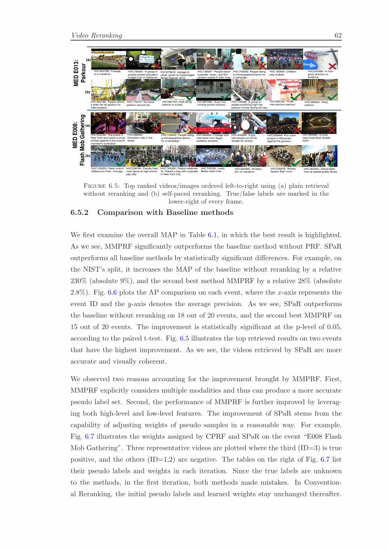
Video Reranking 62
HVC523034: The police in New York shut down a small protest against a city council
member's fundraiser
HVC288592:
Education rally in the street.
HVC709059: People doing
a choreographed dance for a campaign .
HVC562609 : Footage and
interviews from Egypt solidarity protests .
HVC635692: A guy
lets people cut off his dreads for charity .
HVC059444: Pro-union
protest in Wisconsin , against the govenor .
HVC383369: A jump
rope troup does double dutch.
HVC103253: Flash mob in
Millennium Park , Chicago .
HVC508163: Faculty flash
mob dance at high school pep rally .
HVC744324: People celebrate
St. Patrick's Day with a parade in New York City .
HVC745339: Justin Bieber flash mob .
HVC824069: Amateur film of marathon .
HVC036225: Britney Spears flash mob .
HVC067623: Dance flash mob at Seattle public library .
HVC264196: People attend a state fair do parkour on
rollercoasters .
HVC179107: Kid does
parkour around city .
HVC667755: Kids doing parkour in a park .
HVC887082 : Guys free running across campus .
HVC135468: A group of people practicing high risk
parkour moves during the day .
HVC595192 : Three men perform parkour .
HVC295234: Philly parkour.
(a)
(b)
(b)
(a)
HVC800786: Footage
of a marathon .HVC745081: A group of
people protest education budget cuts in California .
HVC676818 : footage of urban sports at Copenhagen
Street Festival 2010
HVC196047 : People watch
a parade , leave, and film random events in their lives .
HVC709059: People doing
a choreographed dance for a campaign .
HVC185454: Children
play football .
HVC242096: A main
gives direction to locations.
ME
D E
013
:
Par
ko
ur
ME
D E
008:
Fla
sh M
ob
Gat
her
ing
Figure 6.5: Top ranked videos/images ordered left-to-right using (a) plain retrievalwithout reranking and (b) self-paced reranking. True/false labels are marked in the
lower-right of every frame.
6.5.2 Comparison with Baseline methods
We first examine the overall MAP in Table 6.1, in which the best result is highlighted.
As we see, MMPRF significantly outperforms the baseline method without PRF. SPaR
outperforms all baseline methods by statistically significant differences. For example, on
the NIST’s split, it increases the MAP of the baseline without reranking by a relative
230% (absolute 9%), and the second best method MMPRF by a relative 28% (absolute
2.8%). Fig. 6.6 plots the AP comparison on each event, where the x-axis represents the
event ID and the y-axis denotes the average precision. As we see, SPaR outperforms
the baseline without reranking on 18 out of 20 events, and the second best MMPRF on
15 out of 20 events. The improvement is statistically significant at the p-level of 0.05,
according to the paired t-test. Fig. 6.5 illustrates the top retrieved results on two events
that have the highest improvement. As we see, the videos retrieved by SPaR are more
accurate and visually coherent.
We observed two reasons accounting for the improvement brought by MMPRF. First,
MMPRF explicitly considers multiple modalities and thus can produce a more accurate
pseudo label set. Second, the performance of MMPRF is further improved by leverag-
ing both high-level and low-level features. The improvement of SPaR stems from the
capability of adjusting weights of pseudo samples in a reasonable way. For example,
Fig. 6.7 illustrates the weights assigned by CPRF and SPaR on the event “E008 Flash
Mob Gathering”. Three representative videos are plotted where the third (ID=3) is true
positive, and the others (ID=1,2) are negative. The tables on the right of Fig. 6.7 list
their pseudo labels and weights in each iteration. Since the true labels are unknown
to the methods, in the first iteration, both methods made mistakes. In Convention-
al Reranking, the initial pseudo labels and learned weights stay unchanged thereafter.

Video Reranking 63
E06 E07 E08 E09 E10 E11 E12 E13 E14 E15 E21 E22 E23 E24 E25 E26 E27 E28 E29 E300
0.1
0.2
0.3
0.4
0.5
Event ID
Avera
ge P
recis
ion
Without Reranking
Rocchio
Relevance Model
CPRF
Learning to Rank
MMPRF
SPaR (Self−paced Reranking )
Figure 6.6: The AP comparison with the baseline methods. The MAP across allevents is available in Table 6.1.
Flash Mob Gathering
People gather for
some sort
of protest.
-1
-1
HVC789180
Description True Label
ID
1
2
HVC513787
Group of
people
flash
mobbing
outdoors.
+1
Time lapse footage of
everyday
things.HVC861609
3
Conventional Reranking
(CPRF)
iter1
+1 1.0
+1 1.0
-1 0.0
1
2
3
+1 1.0
+1 1.0
-1 0.0
+1 1.0
+1 1.0
-1 0.0
label
iter2
label weight
iter3
label weightweightID
Itera
tion
Self-paced Reranking
(mixture weighting)
iter1
+1 1.0
+1 1.0
-1 0.0
+1 .65
+1 .58
+1 .12
+1 .34
+1 .11
+1 .37
label
iter2
label weight
iter3
label weightweight
1
2
3
ID
Iteration
Figure 6.7: Weights changed by CPRF and SPaR on representative videos in differentiterations.
However, SPaR adaptively adjusts their weights as the iteration grows, e.g. it reduces
the overestimated weights of videos (ID=1,2) in iteration 2 and 3 probably because of
their dissimilarity from other pseudo positive videos.
We found two scenarios where SPaR and MMPRF can fail. First, when the initial top-
ranked samples retrieved by queries are completely off-topic. SPaR and MMPRF may
not recover from the inferior starting values, e.g. the query brought by “E022 Cleaning
an appliance” are off-topic (all videos are on all cooking in kitchen). Second, SPaR and
MMPRF may not help when the features used in reranking are not discriminative to the
queries, e.g. for “E025 Marriage Proposal”, our system lacks of meaningful detectors
such as “stand on knees”. Therefore even if 10 true positives are used, the AP is still
bad.
6.5.3 Impact of Pseudo Label Accuracy
To study the impact of pseudo label accuracy, we conduct the following experiments,
where the pseudo positive samples are simply selected by the top k+ samples in the
ranked lists of individual features and the fusion of all features. Figure 6.8(a) illustrates
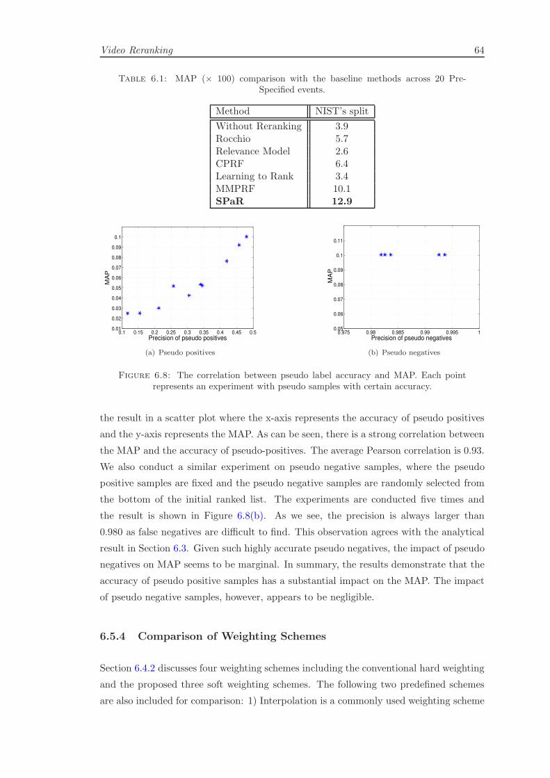
Video Reranking 64
Table 6.1: MAP (× 100) comparison with the baseline methods across 20 Pre-Specified events.
Method NIST’s split
Without Reranking 3.9Rocchio 5.7Relevance Model 2.6CPRF 6.4Learning to Rank 3.4MMPRF 10.1SPaR 12.9
0.1 0.15 0.2 0.25 0.3 0.35 0.4 0.45 0.50.01
0.02
0.03
0.04
0.05
0.06
0.07
0.08
0.09
0.1
Precision of pseudo positives
MA
P
(a) Pseudo positives
0.975 0.98 0.985 0.99 0.995 10.05
0.06
0.07
0.08
0.09
0.1
0.11
Precision of pseudo negatives
MA
P
(b) Pseudo negatives
Figure 6.8: The correlation between pseudo label accuracy and MAP. Each pointrepresents an experiment with pseudo samples with certain accuracy.
the result in a scatter plot where the x-axis represents the accuracy of pseudo positives
and the y-axis represents the MAP. As can be seen, there is a strong correlation between
the MAP and the accuracy of pseudo-positives. The average Pearson correlation is 0.93.
We also conduct a similar experiment on pseudo negative samples, where the pseudo
positive samples are fixed and the pseudo negative samples are randomly selected from
the bottom of the initial ranked list. The experiments are conducted five times and
the result is shown in Figure 6.8(b). As we see, the precision is always larger than
0.980 as false negatives are difficult to find. This observation agrees with the analytical
result in Section 6.3. Given such highly accurate pseudo negatives, the impact of pseudo
negatives on MAP seems to be marginal. In summary, the results demonstrate that the
accuracy of pseudo positive samples has a substantial impact on the MAP. The impact
of pseudo negative samples, however, appears to be negligible.
6.5.4 Comparison of Weighting Schemes
Section 6.4.2 discusses four weighting schemes including the conventional hard weighting
and the proposed three soft weighting schemes. The following two predefined schemes
are also included for comparison: 1) Interpolation is a commonly used weighting scheme

Video Reranking 65
1 2 3 4 50.06
0.07
0.08
0.09
0.1
0.11
0.12
0.13
Iteration Number
Me
an
Ave
rag
e P
recis
ion
Hard Weighting (Binary)
Inverse Rank (Predefined)
Interpolation (Predefined)
Linear Soft Weighting (Learned)
Log Soft Weighting (Learned)
Mixture Weighting (Learned)
Figure 6.9: Comparison of binary, predefined, and learned weighting schemes in dif-ferent iterations.
which assigns weights linearly to a sample’ rank order [94, 105]:
vi =1
m
m∑
j=1
(1− rank(xij)
N), (6.24)
where N is the number of total pseudo samples. The weight for the first sample is 1.0,
and 0.0 for the last. rank(·) returns the sample’s rank order in its list. 2) Inverse Rank
assigns a sample’s weight based on its inverse rank order. The weight vi equals the
average inverse rank across m modalities:
vi =1
m
m∑
j=1
1
rank(xij). (6.25)
We conduct experiments with different weighting schemes and plot their MAPs in
Fig. 6.9, where the x-axis denotes the iteration, and the y-axis is the MAP. The same
step size is used in all methods. As we see, SPaR with the proposed soft weighting
schemes, including linear, log and mixture weighting, outperforms the binary and the
predefined weighting across iterations. Among them, the mixture weighting is slightly
better than others, suggesting the rationale for tolerating small errors on this dataset.
However, it needs an additional parameter to tune. The MAPs of the proposed soft
weighting schemes seem to be robust and less sensitive to the iteration change. The
MAP drop, in all reranking methods, seems to be related to the nature of the MED
dataset as the similar pattern can be observed in other reranking methods. Neverthe-
less, SPaR still outperforms the binary, predefined weights and the baseline methods in
Table 6.1.

Video Reranking 66
6.5.5 Experiments on Hybrid Search
[todo: add more experimental results]
6.5.6 Experiments on Web Query Dataset
To verify SPaR’s performance on image search, we conduct experiments on a web im-
age query dataset consisting of 71,478 images from 353 queries, retrieved by a search
engine named Exalead. For each query, the top ranked images generated by Exalead
are provided, along with the true label for every image. The dataset is representative
as the 353 queries cover a broad range of topics. The performance is evaluated by the
non-interpolated MAP, as used in [90]. MAP@100 is also included for comparison. Note
that as the initial result contains a single modality.
Following [91, 92], densely sampled SIFT are extracted. A codebook of 1,024 centroids
is constructed. Spatial Tiling [121] is used to further improve the performance. We
compare SPaR with the state-of-the-art reranking methods. SPaR is configured in a
similar way as discussed in Section 6.5.1, and provided initial text-based search results
are used. Following [91, 92], the parameters are tuned on a validation set consisting of
a subset of 55 queries.
We examine the overall MAP in Table 6.2. “-” denotes that the number is unavailable
in the cited paper. As we see, SPaR achieves the promising MAP among state-of-the-art
reranking methods, including Graph-based [109], LETOR-based [91, 105], Classification-
based [97] and even supervised reranking methods [90, 107], in terms of both MAP
and MAP@100. A similar pattern can be observed that SPaR significantly boosts the
MAP of plain retrieval without reranking, and obtain comparable or even better perfor-
mance than the baseline methods. Generally, SPaR improves about 84% queries over the
method without reranking. Since the initial ranked lists are retrieved by text matching,
this result substantiates the claim that SPaR is general and applicable to reranking by
text-based search.
6.5.7 Runtime Comparison
To empirically verify the efficiency of SPaR and MMPRF, we compare the runtime
(second/query) in a single iteration. The experiments are conducted on Intel Xeon
E5649 @ 2.53GHz with 16GB memory and the results are listed in Table 6.3. To test
the speed of Rocchio and Relevance Model, we built our own inverted index on the Web
Query dataset, and issue the query against the index. The reranking in MED, which
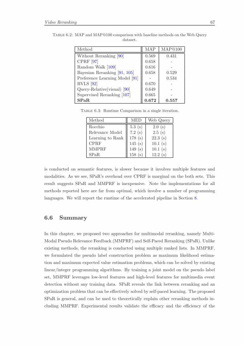
Video Reranking 67
Table 6.2: MAP and MAP@100 comparison with baseline methods on the Web Querydataset.
Method MAP MAP@100
Without Reranking [90] 0.569 0.431CPRF [97] 0.658 -Random Walk [109] 0.616 -Bayesian Reranking [91, 105] 0.658 0.529Preference Learning Model [91] - 0.534BVLS [92] 0.670 -Query-Relative(visual) [90] 0.649 -Supervised Reranking [107] 0.665 -SPaR 0.672 0.557
Table 6.3: Runtime Comparison in a single iteration.
Method MED Web Query
Rocchio 5.3 (s) 2.0 (s)Relevance Model 7.2 (s) 2.5 (s)Learning to Rank 178 (s) 22.3 (s)CPRF 145 (s) 10.1 (s)MMPRF 149 (s) 10.1 (s)SPaR 158 (s) 12.2 (s)
is conducted on semantic features, is slower because it involves multiple features and
modalities. As we see, SPaR’s overhead over CPRF is marginal on the both sets. This
result suggests SPaR and MMPRF is inexpensive. Note the implementations for all
methods reported here are far from optimal, which involve a number of programming
languages. We will report the runtime of the accelerated pipeline in Section 8.
6.6 Summary
In this chapter, we proposed two approaches for multimodal reranking, namely Multi-
Modal Pseudo Relevance Feedback (MMPRF) and Self-Paced Reranking (SPaR). Unlike
existing methods, the reranking is conducted using multiple ranked lists. In MMPRF,
we formulated the pseudo label construction problem as maximum likelihood estima-
tion and maximum expected value estimation problems, which can be solved by existing
linear/integer programming algorithms. By training a joint model on the pseudo label
set, MMPRF leverages low-level features and high-level features for multimedia event
detection without any training data. SPaR reveals the link between reranking and an
optimization problem that can be effectively solved by self-paced learning. The proposed
SPaR is general, and can be used to theoretically explain other reranking methods in-
cluding MMPRF. Experimental results validate the efficacy and the efficiency of the

Video Reranking 68
proposed methods on several datasets. The proposed methods consistently outperforms
the plain retrieval without reranking, and obtains decent improvements over existing
reranking methods.

Chapter 7
Building Semantic Concepts by
Self-paced Curriculum Learning
7.1 Introduction
Concept detectors is the key in a CBVSR system as it not only affects what can be
searched by semantic search but also determines the video representation in hybrid
search. Concept detectors can be trained on still images or videos. The latter is more
desirable due to the minimal domain difference and the capability for action and audio
detection. In this chapter, we explore a semantic concept training method using self-
paced curriculum learning. The theory has been used in the reranking method SPaR in
Section 6.4. In this chapter, we will formally introduce the general form of the theory and
discuss its application on semantic concept training. We approach this problem based on
recently proposed theories called Curriculum learning [98] and self-paced learning [99].
The theories have been attracting increasing attention in the field of machine learning
and artificial intelligence. Both the learning paradigms are inspired by the learning prin-
ciple underlying the cognitive process of humans and animals, which generally start with
learning easier aspects of a task, and then gradually take more complex examples into
consideration. The intuition can be explained in analogous to human education in which
a pupil is supposed to understand elementary algebra before he or she can learn more
advanced algebra topics. This learning paradigm has been empirically demonstrated to
be instrumental in avoiding bad local minima and in achieving a better generalization
result [122–124].
A curriculum determines a sequence of training samples which essentially corresponds
to a list of samples ranked in ascending order of learning difficulty. A major disparity
between curriculum learning (CL) and self-paced learning (SPL) lies in the derivation of
69
Building Semantic Concepts by Self-paced Curriculum Learning 70
the curriculum. In CL, the curriculum is assumed to be given by an oracle beforehand,
and remains fixed thereafter. In SPL, the curriculum is dynamically generated by the
learner itself, according to what the learner has already learned.
The advantage of CL includes the flexibility to incorporate prior knowledge from various
sources. Its drawback stems from the fact that the curriculum design is determined in-
dependently of the subsequent learning, which may result in inconsistency between the
fixed curriculum and the dynamically learned models. From the optimization perspec-
tive, since the learning proceeds iteratively, there is no guarantee that the predetermined
curriculum can even lead to a converged solution. SPL, on the other hand, formulates
the learning problem as a concise biconvex problem, where the curriculum design is
embedded and jointly learned with model parameters. Therefore, the learned model is
consistent. However, SPL is limited in incorporating prior knowledge into learning, ren-
dering it prone to overfitting. Ignoring prior knowledge is less reasonable when reliable
prior information is available. Since both methods have their advantages, it is difficult
to judge which one is better in practice.
In this chapter, we discover the missing link between CL and SPL. We formally propose
a unified framework called Self-paced Curriculum Leaning (SPCL). SPCL represents a
general learning paradigm that combines the merits from both the CL and SPL. On
one hand, it inherits and further generalizes the theory of SPL. On the other hand,
SPCL addresses the drawback of SPL by introducing a flexible way to incorporate prior
knowledge. This chapter offers a compelling insight on the relationship between the
existing CL and SPL methods. Their relation can be intuitively explained in the context
of human education, in which SPCL represents an “instructor-student collaborative”
learning paradigm, as opposed to “instructor-driven” in CL or “student-driven” in SPL.
In SPCL, instructors provide prior knowledge on a weak learning sequence of samples,
while leaving students the freedom to decide the actual curriculum according to their
learning pace. Since an optimal curriculum for the instructor may not necessarily be
optimal for all students, we hypothesize that given reasonable prior knowledge, the
curriculum devised by instructors and students together can be expected to be better
than the curriculum designed by either part alone.
Building Semantic Concepts by Self-paced Curriculum Learning 71
7.2 Related Work
7.2.1 Curriculum Learning
Bengio et al. proposed a new learning paradigm called curriculum learning (CL), in
which a model is learned by gradually including from easy to complex samples in train-
ing so as to increase the entropy of training samples [98]. Afterwards, Bengio and his
colleagues presented insightful explorations for the rationality underlying this learning
paradigm, and discussed the relationship between CL and conventional optimization
techniques, e.g., the continuation and annealing methods [125, 126]. From human be-
havioral perspective, evidence have shown that CL is consistent with the principle in
human teaching [122, 123].
The CL methodology has been applied to various applications, the key in which is to find
a ranking function that assigns learning priorities to training samples. Given a training
set D = (xi, yi)ni=1, where xi denotes the ith observed sample, and yi represents its
label. A curriculum is characterized by a ranking function γ. A sample with a higher
rank, i.e., smaller value, is supposed to be learned earlier.
The curriculum (or the ranking function) is often derived by predetermined heuristics
for particular problems. For example, in the task of classifying geometrical shapes, the
ranking function was derived by the variability in shape [98]. The shapes exhibiting less
variability are supposed to be learned earlier. In [122], the authors tried to teach a robot
the concept of “graspability” - whether an object can be grasped and picked up with
one hand, in which participants were asked to assign a learning sequence of graspability
to various object. The ranking is determined by common sense of the participants.
In [127], the authors approached grammar induction, where the ranking function is
derived in terms of the length of a sentence. The heuristic is that the number of possible
solutions grows exponentially with the length of the sentence, and short sentences are
easier and thus should be learn earlier.
The heuristics in these problems turn out to be beneficial. However, the heuristical
curriculum design may lead to inconsistency between the fixed curriculum and the dy-
namically learned models. That is, the curriculum is predetermined a priori and cannot
be adjusted accordingly, taking into account the feedback about the learner.
7.2.2 Self-paced Learning
To alleviate the issue of CL, Koller’s group [99] designed a new formulation, called self-
paced learning (SPL). SPL embeds curriculum design as a regularization term into the
Building Semantic Concepts by Self-paced Curriculum Learning 72
learning objective. Compared with CL, SPL exhibits two advantages: first, it jointly
optimizes the learning objective together with the curriculum, and therefore the curricu-
lum and the learned model are consistent under the same optimization problem; second,
the regularization term is independent of loss functions of specific problems. This theory
has been successfully applied to various applications, such as action/event detection [70],
reranking [14], domain adaption [124], dictionary learning [128], tracking [129] and seg-
mentation [130].
Formally, let L(yi, g(xi,w)) denote the loss function which calculates the cost between
the ground truth label yi and the estimated label g(xi,w). Here w represents the model
parameter inside the decision function g. In SPL, the goal is to jointly learn the model
parameter w and the latent weight variable v = [v1, · · · , vn]T by minimizing:
minw,v∈[0,1]n
E(w,v;λ)=
n∑
i=1
viL(yi, g(xi,w))−λn∑
i=1
vi, (7.1)
where λ is a parameter for controlling the learning pace. Eq. (7.1) indicates the loss of
a sample is discounted by a weight. The objective of SPL is to minimize the weighted
training loss together with the negative l1-norm regularizer −‖v‖1 = −∑ni=1 vi (since
vi ≥ 0). A more general regularizer consists of both ‖v‖1 and the sum of group-wise
‖v‖2 [70].
ACS (Alternative Convex Search) is generally used to solve Eq. (7.1) [112]. ACS is a
special case of Cyclic Coordinate Method (CCM) [112] discussed in Section 6.4. It is an
iterative method for biconvex optimization, in which the variables are divided into two
disjoint blocks. In each iteration, a block of variables are optimized while keeping the
other block fixed. With the fixed w, the global optimum v∗ = [v∗1 , · · · , v∗n] can be easily
calculated by:
v∗i =
1, L(yi, g(xi,w)) < λ,
0, otherwise.(7.2)
There exists an intuitive explanation behind this alternative search strategy: first, when
updating v with a fixed w, a sample whose loss is smaller than a certain threshold λ
is taken as an “easy” sample, and will be selected in training (v∗i = 1), or otherwise
unselected (v∗i = 0); second, when updating w with a fixed v, the classifier is trained
only on the selected “easy” samples. The parameter λ controls the pace at which the
model learns new samples, and physically λ corresponds to the “age” of the model.
When λ is small, only “easy” samples with small losses will be considered. As λ grows,
more samples with larger losses will be gradually appended to train a more “mature”
model.

Building Semantic Concepts by Self-paced Curriculum Learning 73
This strategy complies with the heuristics in most CL methods [98, 122]. However, since
the learning is completely dominated by the training loss, the learning may be prone
to overfitting. Moreover, it provides no way to incorporate prior guidance in learning.
To the best of our knowledge, there has been no studies to incorporate prior knowledge
into SPL, nor to analyze the relation between CL and SPL.
7.2.3 Survey on Weakly Training
[add the survey of training concept detectors using web data]
7.3 Theory
7.3.1 Model
An ideal learning paradigm should consider both prior knowledge known before training
and information learned during training in a unified and sound framework. Similar to
human education, we are interested in constructing an “instructor-student collabora-
tive” paradigm, which, on one hand, utilizes prior knowledge provided by instructors as
a guidance for curriculum design (the underlying CL methodology), and, on the other
hand, leaves students certain freedom to adjust to the actual curriculum according to
their learning paces (the underlying SPL methodology). This requirement can be re-
alized through the following optimization model. Similar in CL, we assume that the
model is given a curriculum that is predetermined by an oracle. Following the notation
defined above, we have:
minw,v∈[0,1]n
E(w,v;λ,Ψ)=
n∑
i=1
viL(yi,g(xi,w))+f(v;λ)
s.t. v ∈ Ψ
(7.3)
where v = [v1, v2, · · · , vn]T denote the weight variables reflecting the samples’ impor-
tance. f is called self-paced function which controls the learning scheme; Ψ is a feasible
region that encodes the information of a predetermined curriculum. A curriculum can
be mathematically described as:
Definition 7.1 (Total order curriculum). For training samples X = xini=1, a total
order curriculum, or curriculum for short, can be expressed as a ranking function:
γ : X→ 1, 2, · · · , n,
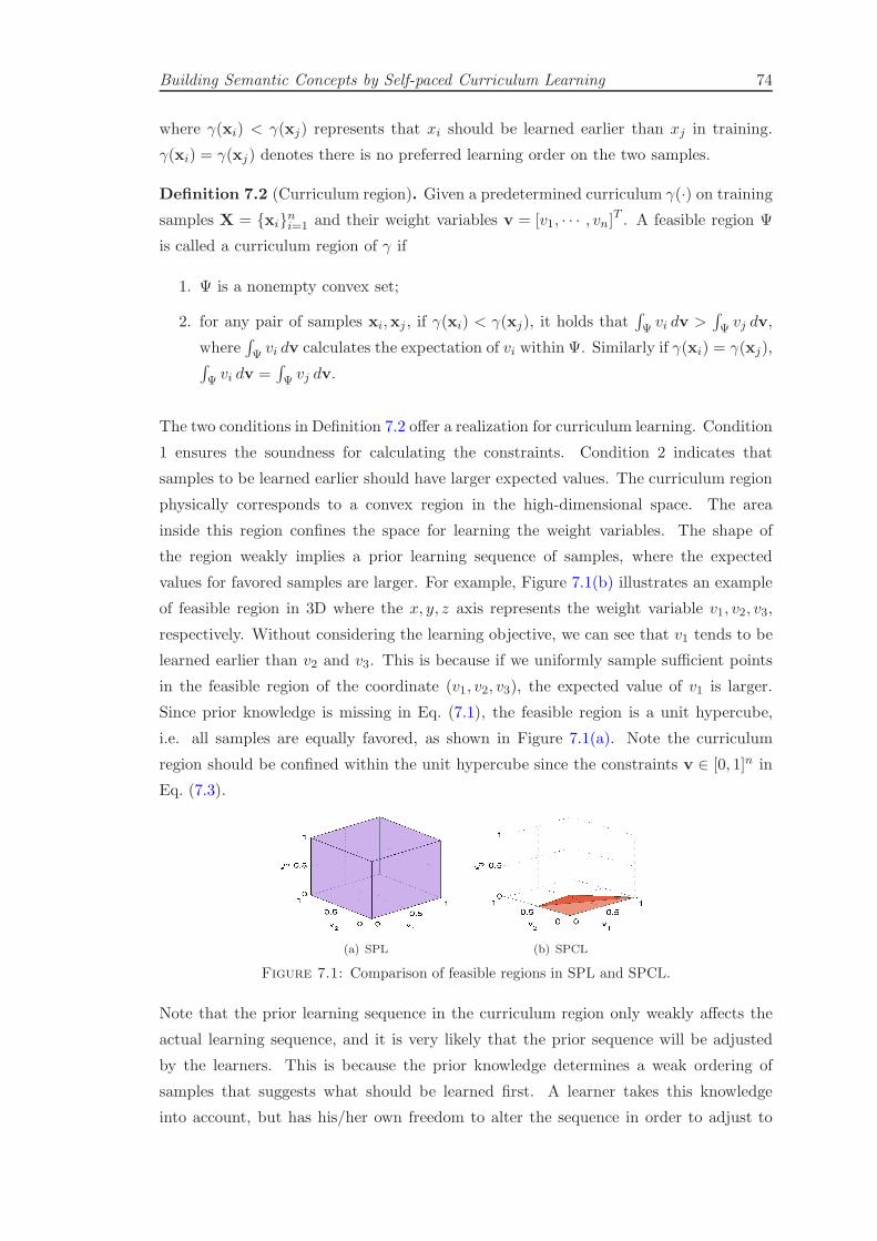
Building Semantic Concepts by Self-paced Curriculum Learning 74
where γ(xi) < γ(xj) represents that xi should be learned earlier than xj in training.
γ(xi) = γ(xj) denotes there is no preferred learning order on the two samples.
Definition 7.2 (Curriculum region). Given a predetermined curriculum γ(·) on training
samples X = xini=1 and their weight variables v = [v1, · · · , vn]T . A feasible region Ψ
is called a curriculum region of γ if
1. Ψ is a nonempty convex set;
2. for any pair of samples xi,xj , if γ(xi) < γ(xj), it holds that∫Ψ vi dv >
∫Ψ vj dv,
where∫Ψ vi dv calculates the expectation of vi within Ψ. Similarly if γ(xi) = γ(xj),∫
Ψ vi dv =∫Ψ vj dv.
The two conditions in Definition 7.2 offer a realization for curriculum learning. Condition
1 ensures the soundness for calculating the constraints. Condition 2 indicates that
samples to be learned earlier should have larger expected values. The curriculum region
physically corresponds to a convex region in the high-dimensional space. The area
inside this region confines the space for learning the weight variables. The shape of
the region weakly implies a prior learning sequence of samples, where the expected
values for favored samples are larger. For example, Figure 7.1(b) illustrates an example
of feasible region in 3D where the x, y, z axis represents the weight variable v1, v2, v3,
respectively. Without considering the learning objective, we can see that v1 tends to be
learned earlier than v2 and v3. This is because if we uniformly sample sufficient points
in the feasible region of the coordinate (v1, v2, v3), the expected value of v1 is larger.
Since prior knowledge is missing in Eq. (7.1), the feasible region is a unit hypercube,
i.e. all samples are equally favored, as shown in Figure 7.1(a). Note the curriculum
region should be confined within the unit hypercube since the constraints v ∈ [0, 1]n in
Eq. (7.3).
(a) SPL (b) SPCL
Figure 7.1: Comparison of feasible regions in SPL and SPCL.
Note that the prior learning sequence in the curriculum region only weakly affects the
actual learning sequence, and it is very likely that the prior sequence will be adjusted
by the learners. This is because the prior knowledge determines a weak ordering of
samples that suggests what should be learned first. A learner takes this knowledge
into account, but has his/her own freedom to alter the sequence in order to adjust to

Building Semantic Concepts by Self-paced Curriculum Learning 75
Table 7.1: Comparison of different learning approaches.
CL SPL Proposed SPCLComparable to human learning Instructor-driven Student-driven Instructor-student collaborative
Curriculum design Prior knowledge Learning objective Learning objective + prior knowledgeLearning schemes Multiple Single MultipleIterative training Heuristic approach Gradient-based Gradient-based
the learning objective. See Example 7.1. Therefore, SPCL represents an “instructor-
student-corporative” learning paradigm.
Compared with Eq. (7.1), SPCL generalizes SPL by introducing a regularization term.
This term determines the learning scheme, i.e., the strategy used by the model to learn
new samples. In human learning, we tend to use different schemes for different tasks.
Similarly, SPCL should also be able to utilize different learning schemes for different
problems. Since the existing methods only include a single learning scheme, we generalize
the learning scheme and define:
Definition 7.3 (Self-paced function). A self-paced function determines a learning scheme.
Suppose that v = [v1, · · · , vn]T denotes a vector of weight variable for each training sam-
ple and ℓ = [ℓ1, · · · , ℓn]T are the corresponding loss. λ controls the learning pace (or
model “age”). f(v;λ) is called a self-paced function, if
1. f(v;λ) is convex with respect to v ∈ [0, 1]n.
2. When all variables are fixed except for vi and ℓi, v∗i decreases with ℓi, and it holds
that limℓi→0
v∗i = 1, limℓi→∞
v∗i = 0.
3. ‖v‖1 =∑n
i=1 vi increases with respect to λ, and it holds that ∀i∈ [1, n], limλ→0
v∗i =
0, limλ→∞
v∗i =1.
where v∗ = argminv∈[0,1]n∑
viℓi + f(v;λ), and denote v∗ = [v∗1 , · · · , v∗n].
The three conditions in Definition 7.3 provide a definition for the self-paced learning
scheme. Condition 2 indicates that the model inclines to select easy samples (with
smaller losses) in favor of complex samples (with larger losses). Condition 3 states that
when the model “age” λ gets larger, it should incorporate more, probably complex,
samples to train a “mature” model. The convexity in Condition 1 ensures the model
can find good solutions within the curriculum region.
It is easy to verify that the regularization term in Eq. (7.1) satisfies Definition 7.3. In fact,
this term corresponds to a binary learning scheme since vi can only take binary values,
as shown in the closed-form solution of Eq. (7.2). This scheme may be less appropriate
in the problems where the importance of samples needs to be discriminated. In fact,

Building Semantic Concepts by Self-paced Curriculum Learning 76
there exist a plethora of self-paced functions corresponding to various learning schemes.
We will detail some of them in the next section.
Inspired by the algorithm in [99], we employ a similar ACS algorithm to solve Eq. (7.3).
Algorithm 2 takes the input of a predetermined curriculum, an instantiated self-paced
function and a stepsize parameter; it outputs an optimal model parameterw. First of all,
it represents the input curriculum as a curriculum region that follows Definition 2, and
initializes variables in their feasible region. Then it alternates between two steps until
it finally converges: Step 4 learns the optimal model parameter with the fixed and most
recent v∗; Step 5 learns the optimal weight variables with the fixed w∗. In first several
iterations, the model “age” is increased so that more complex samples will be gradually
incorporated in the training. For example, we can increase λ so that µ more samples will
be added in the next iteration. According to the conditions in Definition 7.3, the number
of complex samples increases along with the growth of the number iteration. Step 4
can be conveniently implemented by existing off-the-shelf supervised learning methods.
Gradient-based or interior-point methods can be used to solve the convex optimization
problem in Step 5. According to [112], the alternative search in Algorithm 2 converges
as the objective function is monotonically decreasing and is bounded from below.
Algorithm 2: Self-paced Curriculum Learning.
input : Input dataset D, predetermined curriculum γ, self-paced function f and astepsize µ
output: Model parameter w
1 Derive the curriculum region Ψ from γ;2 Initialize v∗, λ in the curriculum region;3 while not converged do4 Update w∗ = argminw E(w,v∗;λ,Ψ);5 Update v∗ = argminv E(w
∗,v;λ,Ψ);6 if λ is small then increase λ by the stepsize µ;
7 end8 return w∗
7.3.2 Relationship to CL and SPL
SPCL represents a general learning framework which includes CL and SPL as special
cases. SPCL degenerates to SPL when the curriculum region is ignored (Ψ = [0, 1]n),
or equivalently, the prior knowledge on predefined curriculums is absent. In this case,
the learning is totally driven by the learner. SPCL degenerates to CL when the curricu-
lum region (feasible region) only contains the learning sequence in the predetermined
curriculum. In this case, the learning process neglects the feedback about learners, and
is dominated by the given prior knowledge. When information from both sources are
Building Semantic Concepts by Self-paced Curriculum Learning 77
available, the learning in SPCL is collaboratively driven by prior knowledge and learning
objective. Table 7.1 summarizes the characteristics of different learning methods. Given
reasonable prior knowledge, SPCL which considers the information from both sources
tend to yield better solutions. Example 7.1 shows a case in this regard.
7.3.3 Implementation
The definitions discussed above provide a theoretical foundation for SPCL. However, we
still need concrete self-paced functions and curriculum regions to solve specific problems.
To this end, this section discusses some implementations that follow Definition 7.2 and
Definition 7.3. Note that there is no single implementation that can always work the
best for all problems. Our purpose is to argument the implementations in the literature,
and to help enlighten others to further explore this interesting direction.
Curriculum region implementation: We suggest an implementation induced from
a linear constraint for realizing the curriculum region: aTv ≤ c, where v = [v1, · · · , vn]T
are the weight variables in Eq. (7.3), c is a constant, and a = [a1, · · · , an]T is a n-
dimensional vector. The linear constraints is a simple implementation for curriculum
region that can be conveniently solved. It can be proved that this implementation
complies with the definition of curriculum region.
Theorem 7.4. For training samples X = xini=1, given a curriculum γ defined on it,
the feasible region, defined by,
Ψ = v|aTv ≤ c
is a curriculum region of γ if it holds: 1) Ψ ∧ v ∈ [0, 1]n is nonempty; 2) ai<aj for all
γ(xi)<γ(xj); ai=aj for all γ(xi)=γ(xj).
Self-paced function implementation: Similar to the scheme human used to absorb
knowledge, a self-paced function determines a learning scheme for the model to learn
new samples. Note the self-paced function is realized as a regularization term, which
is independent of specific loss functions, and can be easily applied to various problems.
Since human tends to use different learning schemes for different tasks, SPCL should
also be able to utilize different learning schemes for different problems. Inspired by a
study in [14], this section discusses some examples of learning schemes.
Binary scheme: This scheme in is used in [99]. It is called binary scheme, or “hard”
scheme, as it only yields binary weight variables.
f(v;λ) = −λ‖v‖1 = −λn∑
i=1
vi, (7.4)

Building Semantic Concepts by Self-paced Curriculum Learning 78
Linear scheme: A common approach is to linearly discriminate samples with respect to
their losses. This can be realized by the following self-paced function:
f(v;λ) =1
2λ
n∑
i=1
(v2i − 2vi), (7.5)
in which λ > 0. This scheme represents a “soft” scheme as the weight variable can take
real values.
Logarithmic scheme: A more conservative approach is to penalize the loss logarithmi-
cally, which can be achieved by the following function:
f(v;λ) =n∑
i=1
ζvi −ζvi
log ζ, (7.6)
where ζ = 1− λ and 0 < λ < 1.
Mixture scheme: Mixture scheme is a hybrid of the “soft” and the “hard” scheme [14].
If the loss is either too small or too large, the “hard” scheme is applied. Otherwise, the
soft scheme is applied. Compared with the “soft” scheme, the mixture scheme tolerates
small errors up to a certain point. To define this starting point, an additional parameter
is introduced, i.e. λ = [λ1, λ2]T . Formally,
f(v;λ) = −ζn∑
i=1
log(vi +1
λ1ζ), (7.7)
where ζ = λ1λ2λ1−λ2
and λ1 > λ2 > 0.
Theorem 7.5. The binary, linear, logarithmic and mixture scheme function are self-
paced functions.
It can be proved that the above functions follow Definition 7.3. The name of the learning
scheme suggests the characteristic of its solution. The curve in Fig. 6.4 illustrates the
characteristics of the learning schemes. When the curriculum region is not a unit hyper-
cube, the closed-form solution, such as Eq. (7.2) cannot be directly used. Gradient-based
methods can be applied. As Ew is convex, the local optimal is also the global optimal
solution for the subproblem.
Example 7.1. Given six samples a, b, c, d, e, f . In the current iteration, the losses for
these samples are ℓ = [0.1, 0.2, 0.4, 0.6, 0.5, 0.3], respectively. A latent ground-truth cur-
riculum is listed in the first row of the following table, followed by the curriculum of
CL, SPL and SPCL. For simplicity, binary scheme is used in SPL and SPCL where
λ = 0.8333. If two samples with the same weight, we rank them in ascending order of
their losses, in order to break the tie. The Kendall’s rank correlation is presented in the
last column.

Building Semantic Concepts by Self-paced Curriculum Learning 79
Method Curriculum Correlation
Ground-Truth a, b, c, d, e, f -
CL b, a, d, c, e, f 0.73
SPL a, b, f, c, e, d 0.46
SPCL a, b, c, d, e, f 1.00
The curriculum region used is a linear constraint aTv ≤ 1, where a = [0.1, 0.0, 0.4, 0.3, 0.5, 1.0]T .
In the implementation, we add a small constant 10−7 in the constraints for optimiza-
tion accuracy. The constraint follows Definition 2 in the paper. As shown, both CL
and SPL yield the suboptimal curriculum, e.g. their correlations are only 0.73 and
0.46. However, SPCL exploits the complementary information in CL and SPL, and
devises an optimal curriculum. Note that CL recommends to learn b before a, but
SPCL disobeys this order in the actual curriculum. The final solution of SPCL is
v∗ = [1.00, 1.00, 1.00, 0.88, 0.47, 0.00].
When the predetermined curriculum is completely wrong, SPCL may still be robust to
the inferior prior knowledge given reasonable curriculum regions are applied. In this
case, the prior knowledge should not be encoded as strong constraints. For example, in
the above example, we can use the following curriculum region to encode the completely
incorrect predetermined curriculum: aTv ≤ 6.0, where a = [2.3, 2.2, 2.1, 2.0, 1.7, 1.5]T
Method Curriculum Correlation
CL f, e, d, c, b, a -1.00
SPL a, b, f, c, e, d 0.46
SPCL a, f, b, c, e, d 0.33
As we see, even though the predetermined curriculum is completely wrong (correlation
-1.00), the proposed SPCL still obtains reasonable curriculum (correlation 0.33). This
is because SPCL is able to leverage information in both prior knowledge and learning
objective. The optimal solution of SPCL is v∗ = [1.00, 0.91, 0.10, 0.00, 0.00, 1.00].
In the above learning schemes, samples in a curriculum are selected solely in terms of
“easiness”. In this section, we reveal that diversity, an important aspect in learning,
should also be considered. Ideal learning should utilize not only easy but also diverse
examples that are sufficiently dissimilar from what has already been learned. This can
be intuitively explained in the context of human education. A rational curriculum for a
pupil not only needs to include examples of suitable easiness matching her learning pace,
but also, importantly, should include some diverse examples on the subject in order for
her to develop more comprehensive knowledge. Likewise, learning from easy and diverse
samples is expected to be better than learning from either criterion alone. To this end,
we propose the following learning scheme.

Building Semantic Concepts by Self-paced Curriculum Learning 80
Diverse learning scheme: Diversity implies that the selected samples should be less
similar or clustered. An intuitive approach for realizing this is by selecting samples of
different groups scattered in the sample space. We assume that the correlation of samples
between groups is less than that of within a group. This auxiliary group membership
is either given, e.g. in object recognition frames from the same video can be regarded
from the same group, or can be obtained by clustering samples.
This aim can be mathematically described as follows. Assume that the training samples
X = (x1, · · · ,xn) ∈ Rm×n are partitioned into b groups: X(1), · · · ,X(b), where columns
of X(j) ∈ Rm×nj correspond to the samples in the jth group, nj is the sample number in
the group and∑b
j=1 nj = n. Accordingly denote the weight vector as v = [v(1), · · · ,v(b)],
where v(j) = (v(j)1 , · · · , v(j)nj )
T ∈ [0, 1]nj . The diverse learning scheme on one hand needs
to assign nonzero weights of v to easy samples as the hard learning scheme, and on
the other hand requires to disperse nonzero elements across possibly more groups v(i) to
increase the diversity. Both requirements can be uniformly realized through the following
optimization model:
minw,v
E(w,v;λ, γ) =
n∑
i=1
viL(yi, f(xi,w))− λ
n∑
i=1
vi − γ‖v‖2,1, s.t. v ∈ [0, 1]n, (7.8)
where λ, γ are the parameters imposed on the easiness term (the negative l1-norm:
−‖v‖1) and the diversity term (the negative l2,1-norm: −‖v‖2,1), respectively. As for
the diversity term, we have:
− ‖v‖2,1 = −b∑
j=1
‖v(j)‖2. (7.9)
The new regularization term consists of two components. One is the negative l1-norm
inherited from the hard learning scheme in SPL, which favors selecting easy over complex
examples. The other is the proposed negative l2,1-norm, which favors selecting diverse
samples residing in more groups. It is well known that the l2,1-norm leads to the group-
wise sparse representation of v [64], i.e. non-zero entries of v tend to be concentrated in
a small number of groups. Contrariwise, the negative l2,1-norm should have a counter-
effect to group-wise sparsity, i.e. nonzero entries of v tend to be scattered across a large
number of groups. In other words, this anti-group-sparsity representation is expected to
realize the desired diversity. Note that when each group only contains a single sample,
Eq. (D.16) degenerates to Eq. (7.1).
Unlike the convex regularization term above, the term in diverse learning scheme is non-
convex. A challenge is optimizing v with a fixed w becoming a non-convex problem. To
this end, we propose a simple yet effective algorithm for extracting the global optimum
of this problem when the curriculum is as in SPL, i.e. Ψ = [0, 1]n. Algorithm 3 takes
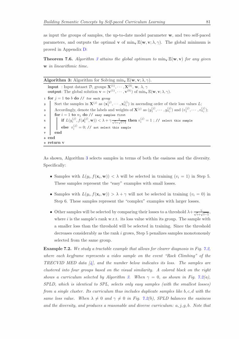
Building Semantic Concepts by Self-paced Curriculum Learning 81
as input the groups of samples, the up-to-date model parameter w, and two self-paced
parameters, and outputs the optimal v of minv E(w,v;λ, γ). The global minimum is
proved in Appendix D:
Theorem 7.6. Algorithm 3 attains the global optimum to minv E(w,v) for any given
w in linearithmic time.
Algorithm 3: Algorithm for Solving minv E(w,v;λ, γ).
input : Input dataset D, groups X(1), · · · ,X(b), w, λ, γoutput: The global solution v = (v(1), · · · ,v(b)) of minv E(w,v;λ, γ).
1 for j = 1 to b do // for each group
2 Sort the samples in X(j) as (x(j)1 , · · · ,x(j)
nj ) in ascending order of their loss values L;
3 Accordingly, denote the labels and weights of X(j) as (y(j)1 , · · · , y(j)nj ) and (v
(j)1 , · · · , v(j)nj );
4 for i = 1 to nj do // easy samples first
5 if L(y(j)i , f(x
(j)i ,w)) < λ+ γ 1√
i+√i−1
then v(j)i = 1 ; // select this sample
6 else v(j)i = 0; // not select this sample
7 end
8 end9 return v
As shown, Algorithm 3 selects samples in terms of both the easiness and the diversity.
Specifically:
• Samples with L(yi, f(xi,w)) < λ will be selected in training (vi = 1) in Step 5.
These samples represent the “easy” examples with small losses.
• Samples with L(yi, f(xi,w)) > λ + γ will not be selected in training (vi = 0) in
Step 6. These samples represent the “complex” examples with larger losses.
• Other samples will be selected by comparing their losses to a threshold λ+ γ√i+
√i−1
,
where i is the sample’s rank w.r.t. its loss value within its group. The sample with
a smaller loss than the threshold will be selected in training. Since the threshold
decreases considerably as the rank i grows, Step 5 penalizes samples monotonously
selected from the same group.
Example 7.2. We study a tractable example that allows for clearer diagnosis in Fig. 7.2,
where each keyframe represents a video sample on the event “Rock Climbing” of the
TRECVID MED data [4], and the number below indicates its loss. The samples are
clustered into four groups based on the visual similarity. A colored block on the right
shows a curriculum selected by Algorithm 3. When γ = 0, as shown in Fig. 7.2(a),
SPLD, which is identical to SPL, selects only easy samples (with the smallest losses)
from a single cluster. Its curriculum thus includes duplicate samples like b, c, d with the
same loss value. When λ 6= 0 and γ 6= 0 in Fig. 7.2(b), SPLD balances the easiness
and the diversity, and produces a reasonable and diverse curriculum: a, j, g, b. Note that

Building Semantic Concepts by Self-paced Curriculum Learning 82
0.05 0.12
0.12 0.40
0.20
0.18
0.17
0.50
Outdoor bouldering
Artificial wall climbing Snow mountain climbing
0.15
0.35
0.15
0.16
0.28
Bear climbing
a rock
a c e
b d fn
g
hi
j l
k m
0.12a c e
b d fn
g
hi
j l
k m
a c e
b d fn
g
hi
j l
k m
a
b
c
d
e
f
g
h
i
j
k
l
m
n
Curriculum: a, b, c, d
Curriculum: a, j, g, b
Curriculum: a, j, g, n
(a)
(b)
(c)
Figure 7.2: An example on samples selected by Algorithm 3. A colored block denotesa curriculum with given λ and γ, and the bold (red) box indicates the easy sample
selected by Algorithm 3.
even if there exist 3 duplicate samples b, c, d, SPLD only selects one of them due to the
decreasing threshold in Step 5 of Algorithm 3. Likewise, samples e and j share the same
loss, but only j is selected as it is better in increasing the diversity. In an extreme case
where λ = 0 and γ 6= 0, as illustrated in Fig. 7.2(c), SPLD selects only diverse samples,
and thus may choose outliers, such as the sample n which is a confusable video about
a bear climbing a rock. Therefore, considering both easiness and diversity seems to be
more reasonable than considering either one alone. Physically the parameters λ and γ
together correspond to the “age” of the model, where λ focuses on easiness whereas γ
stresses diversity.
7.3.4 Limitations and Practical Observations
We observed a number of limitations of the current SPCL model. First, the fundamental
learning philosophy of SPL/CL/SPCL is 1) learning needs to be conducted iteratively
using samples organized in a meaningful sequence; 2) models are becoming more com-
plex in each iteration. However, the learning philosophy may not applicable to every
learning problem. For example, in many problems where training data, especially s-
mall training data, are are carefully selected and the spectrum of learning difficulty
of training samples is controlled. We found the proposed theory may not outperform
the conventional training methods. Second, the performance of SPCL can be unstable
to the random starting values. This phenomenon can be intuitively explained in the
context of education, it is impossible for students to predetermine what to learn before
they actually learning anything. To address this, the curriculum needs to be meaningful
so that it can provide some supervision in the first few iterations. However, precisely
deriving curriculum region from prior knowledge seems to be an open question. Third,
the age parameters λ are very important hyperparameters to tune. In order to tune the
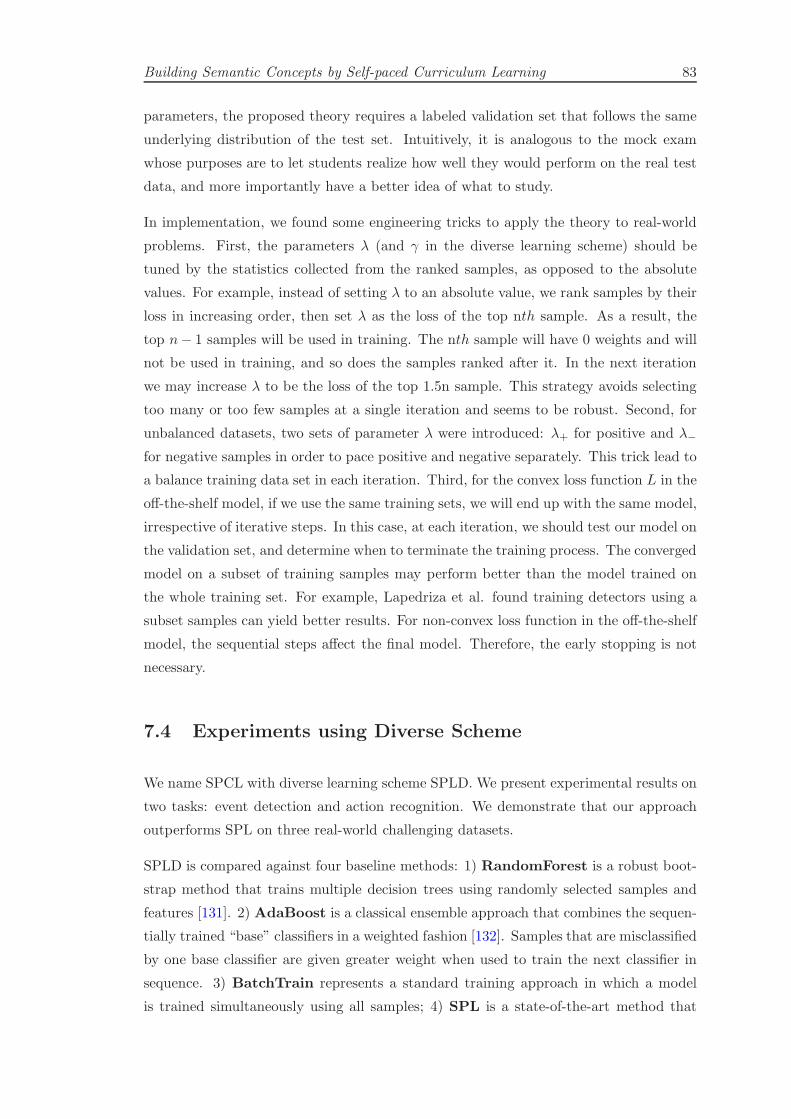
Building Semantic Concepts by Self-paced Curriculum Learning 83
parameters, the proposed theory requires a labeled validation set that follows the same
underlying distribution of the test set. Intuitively, it is analogous to the mock exam
whose purposes are to let students realize how well they would perform on the real test
data, and more importantly have a better idea of what to study.
In implementation, we found some engineering tricks to apply the theory to real-world
problems. First, the parameters λ (and γ in the diverse learning scheme) should be
tuned by the statistics collected from the ranked samples, as opposed to the absolute
values. For example, instead of setting λ to an absolute value, we rank samples by their
loss in increasing order, then set λ as the loss of the top nth sample. As a result, the
top n− 1 samples will be used in training. The nth sample will have 0 weights and will
not be used in training, and so does the samples ranked after it. In the next iteration
we may increase λ to be the loss of the top 1.5n sample. This strategy avoids selecting
too many or too few samples at a single iteration and seems to be robust. Second, for
unbalanced datasets, two sets of parameter λ were introduced: λ+ for positive and λ−
for negative samples in order to pace positive and negative separately. This trick lead to
a balance training data set in each iteration. Third, for the convex loss function L in the
off-the-shelf model, if we use the same training sets, we will end up with the same model,
irrespective of iterative steps. In this case, at each iteration, we should test our model on
the validation set, and determine when to terminate the training process. The converged
model on a subset of training samples may perform better than the model trained on
the whole training set. For example, Lapedriza et al. found training detectors using a
subset samples can yield better results. For non-convex loss function in the off-the-shelf
model, the sequential steps affect the final model. Therefore, the early stopping is not
necessary.
7.4 Experiments using Diverse Scheme
We name SPCL with diverse learning scheme SPLD. We present experimental results on
two tasks: event detection and action recognition. We demonstrate that our approach
outperforms SPL on three real-world challenging datasets.
SPLD is compared against four baseline methods: 1) RandomForest is a robust boot-
strap method that trains multiple decision trees using randomly selected samples and
features [131]. 2) AdaBoost is a classical ensemble approach that combines the sequen-
tially trained “base” classifiers in a weighted fashion [132]. Samples that are misclassified
by one base classifier are given greater weight when used to train the next classifier in
sequence. 3) BatchTrain represents a standard training approach in which a model
is trained simultaneously using all samples; 4) SPL is a state-of-the-art method that

Building Semantic Concepts by Self-paced Curriculum Learning 84
trains models gradually from easy to more complex samples [99]. The baseline methods
are a mixture of the well-known and the state-of-the-art methods on training models
using sampled data.
7.4.1 Event Detection
Given a collection of videos, the goal of MED is to detect events of interest, e.g. “Birth-
day Party” and “Parade”, solely based on the video content. The task is very challenging
due to complex scenes, camera motion, occlusions, etc. The experiments are conducted
on the largest collection on event detection: TRECVID MED13Test, which consists of
about 32,000 Internet videos. There are a total of 3,490 videos from 20 complex events,
and the rest are background videos. For each event 10 positive examples are given to
train a detector, which is tested on about 25,000 videos. The official test split released
by NIST (National Institute of Standards and Technology) is used. A Deep Convolu-
tional Neural Network is trained on 1.2 million ImageNet challenge images from 1,000
classes [75] to represent each video as a 1,000-dimensional vector. Algorithm 3 is used.
By default, the group membership is generated by the spectral clustering, and the num-
ber of groups is set to 64. Following [124], LibLinear is used as the solver in Step 4 of
Algorithm 3 due to its robust performance on this task. The performance is evaluated
using MAP as recommended by NIST. The parameters of all methods are tuned on the
same validation set.
Table 7.2 lists the overall MAP comparison. To reduce the influence brought by ini-
tialization, we repeated experiments of SPL and SPLD 10 times with random starting
values, and report the best run and the mean (with the 95% confidence interval) of the
10 runs. The proposed SPLD outperforms all baseline methods with statistically signif-
icant differences at the p-value level of 0.05, according to the paired t-test. It is worth
emphasizing that MED is very challenging and 26% relative (2.5 absolute) improvement
over SPL is a notable gain. SPLD outperforms other baselines on both the best run
and the 10 runs average. RandomForest and AdaBoost yield poorer performance. This
observation agrees with the study in literature [4] that SVM is more robust on event
detection.
Table 7.2: MAP (x100) comparison with the baseline methods on MED.
Run Name RandomForest AdaBoost BatchTrain SPL SPLDBest Run 3.0 2.8 8.3 9.6 12.1
10 Runs Average 3.0 2.8 8.3 8.6±0.42 9.8±0.45
BatchTrain, SPL and SPLD are all performed using SVM. Regarding the best run,
SPL boosts the MAP of the BatchTrain by a relative 15.6% (absolute 1.3%). SPLD
yields another 26% (absolute 2.5%) over SPL. The MAP gain suggests that optimizing
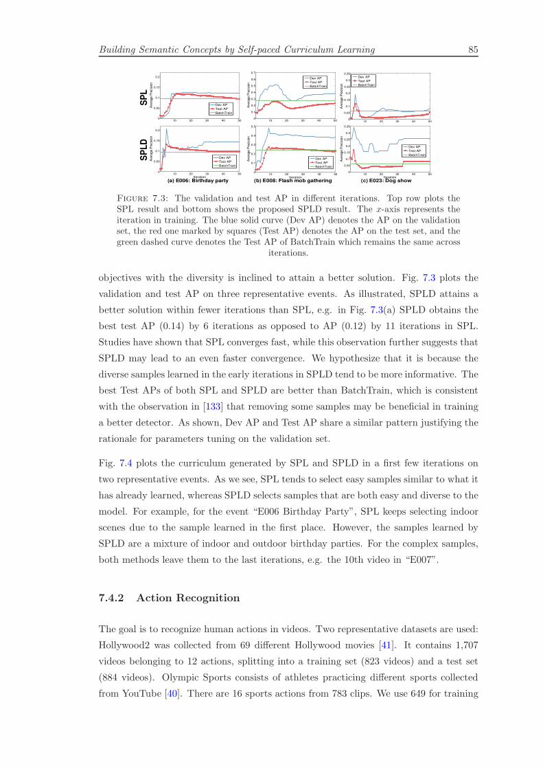
Building Semantic Concepts by Self-paced Curriculum Learning 85
10 20 30 40 500
0.05
0.1
0.15
0.2
Iteration
Ave
rage
Pre
cisi
on
Dev AP
Test AP
BatchTrain
10 20 30 40 500
0.05
0.1
0.15
0.2
Iteration
Ave
rage P
reci
sion
Dev AP
Test AP
BatchTrain
10 20 30 40 500
0.1
0.2
0.3
0.4
0.5
0.6
0.7
Iteration
Ave
rage P
reci
sion
Dev AP
Test AP
BatchTrain
10 20 30 40 500
0.1
0.2
0.3
0.4
0.5
Iteration
Ave
rage P
reci
sion
Dev AP
Test AP
BatchTrain
10 20 30 40 500
0.05
0.1
0.15
0.2
0.25
0.3
0.35
Iteration
Ave
rage P
reci
sion
Dev AP
Test AP
BatchTrain
10 20 30 40 500
0.05
0.1
0.15
0.2
0.25
0.3
0.35
Iteration
Ave
rag
e P
reci
sio
n
Dev AP
Test AP
BatchTrain
(a) E006: Birthday party (b) E008: Flash mob gathering (c) E023: Dog show
SP
LS
PL
D
Figure 7.3: The validation and test AP in different iterations. Top row plots theSPL result and bottom shows the proposed SPLD result. The x-axis represents theiteration in training. The blue solid curve (Dev AP) denotes the AP on the validationset, the red one marked by squares (Test AP) denotes the AP on the test set, and thegreen dashed curve denotes the Test AP of BatchTrain which remains the same across
iterations.
objectives with the diversity is inclined to attain a better solution. Fig. 7.3 plots the
validation and test AP on three representative events. As illustrated, SPLD attains a
better solution within fewer iterations than SPL, e.g. in Fig. 7.3(a) SPLD obtains the
best test AP (0.14) by 6 iterations as opposed to AP (0.12) by 11 iterations in SPL.
Studies have shown that SPL converges fast, while this observation further suggests that
SPLD may lead to an even faster convergence. We hypothesize that it is because the
diverse samples learned in the early iterations in SPLD tend to be more informative. The
best Test APs of both SPL and SPLD are better than BatchTrain, which is consistent
with the observation in [133] that removing some samples may be beneficial in training
a better detector. As shown, Dev AP and Test AP share a similar pattern justifying the
rationale for parameters tuning on the validation set.
Fig. 7.4 plots the curriculum generated by SPL and SPLD in a first few iterations on
two representative events. As we see, SPL tends to select easy samples similar to what it
has already learned, whereas SPLD selects samples that are both easy and diverse to the
model. For example, for the event “E006 Birthday Party”, SPL keeps selecting indoor
scenes due to the sample learned in the first place. However, the samples learned by
SPLD are a mixture of indoor and outdoor birthday parties. For the complex samples,
both methods leave them to the last iterations, e.g. the 10th video in “E007”.
7.4.2 Action Recognition
The goal is to recognize human actions in videos. Two representative datasets are used:
Hollywood2 was collected from 69 different Hollywood movies [41]. It contains 1,707
videos belonging to 12 actions, splitting into a training set (823 videos) and a test set
(884 videos). Olympic Sports consists of athletes practicing different sports collected
from YouTube [40]. There are 16 sports actions from 783 clips. We use 649 for training
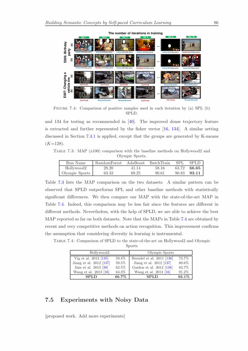
Building Semantic Concepts by Self-paced Curriculum Learning 86
(a)
Iter 1
Indoorbirthday party
...
Iter2 Iter 3
Car/Truck
Iter 4 Iter 9 Iter 10
Indoorbirthday party Indoorbirthday party Indoor birthday party Indoorbirthday party Outdoorbirthday party
Outdoor birthday partyIndoorbirthday party Indoorbirthday party Outdoorbirthday party Indoorbirthday party Indoorbirthday party
...
...
...
Car/Truck
Bicycle/ScooterCar/Truck Bicycle/Scooter Car/Truck
Car/Truck Bicycle/Scooter Bicycle/Scooter
Car/Truck Bicycle/Scooter
(b)
(a)
(b)
E00
6:
Bir
thd
ay
part
y
E007:
Ch
an
gin
g a
veh
icle
tir
e
The number of iterations in training
Car/Truck
Figure 7.4: Comparison of positive samples used in each iteration by (a) SPL (b)SPLD.
and 134 for testing as recommended in [40]. The improved dense trajectory feature
is extracted and further represented by the fisher vector [16, 134]. A similar setting
discussed in Section 7.4.1 is applied, except that the groups are generated by K-means
(K=128).
Table 7.3: MAP (x100) comparison with the baseline methods on Hollywood2 andOlympic Sports.
Run Name RandomForest AdaBoost BatchTrain SPL SPLDHollywood2 28.20 41.14 58.16 63.72 66.65
Olympic Sports 63.32 69.25 90.61 90.83 93.11
Table 7.3 lists the MAP comparison on the two datasets. A similar pattern can be
observed that SPLD outperforms SPL and other baseline methods with statistically
significant differences. We then compare our MAP with the state-of-the-art MAP in
Table 7.4. Indeed, this comparison may be less fair since the features are different in
different methods. Nevertheless, with the help of SPLD, we are able to achieve the best
MAP reported so far on both datasets. Note that the MAPs in Table 7.4 are obtained by
recent and very competitive methods on action recognition. This improvement confirms
the assumption that considering diversity in learning is instrumental.
Table 7.4: Comparison of SPLD to the state-of-the-art on Hollywood2 and OlympicSports
Hollywood2 Olympic Sports
Vig et al. 2012 [135] 59.4% Brendel et al. 2011 [136] 73.7%Jiang et al. 2012 [137] 59.5% Jiang et al. 2012 [137] 80.6%Jain et al. 2013 [39] 62.5% Gaidon et al. 2012 [138] 82.7%Wang et al. 2013 [16] 64.3% Wang et al. 2013 [16] 91.2%
SPLD 66.7% SPLD 93.1%
7.5 Experiments with Noisy Data
[proposed work. Add more experiments]
Building Semantic Concepts by Self-paced Curriculum Learning 87
7.6 Summary
We proposed a novel learning regime called self-paced curriculum learning (SPCL), which
imitates the learning regime of humans/animals that gradually involves from easy to
more complex training samples into the learning process. The proposed SPCL can
exploit both prior knowledge before training and dynamical information extracted during
training. The novel regime is analogous to an “instructor-student-collaborative” learning
mode, as opposed to “instructor-driven” in curriculum learning or “student-driven” in
self-paced learning. We presented compelling understandings for curriculum learning and
self-paced learning, and revealed that they can be unified into a concise optimization
model. We discussed several concrete implementations in the proposed SPCL framework.
SPCL is a general learning framework, the component of which is of physical interpre-
tation. The off-the-shelf models, such as SVMs, deep neural networks, and regression
models, correspond to students. The self-paced functions correspond to learning schemes
used by students to solve specific problems. The curriculum region corresponds to the
prior knowledge provided from an oracle or an instructor so that learning can be pro-
cessed in a desired direction.

Chapter 8
Conclusions and Proposed Work
In this thesis, we studied a fundamental research problem of searching semantic informa-
tion in video content at a very large scale. We proposed several novel methods focusing
on improving accuracy, efficiency and scalability in the novel search paradigm. The pro-
posed methods demonstrated promising results on web-scale semantic search for video.
The extensive experiments demonstrated that the methods are able to surpass state-of-
the-art accuracy on multiple datasets. In addition, our method can efficiently scale up
the search to hundreds of millions videos, and only takes about 0.2 second to search a
semantic query on a collection of 100 million videos, 1 second to process a hybrid query
over 1 million videos. There are two research issues to be addressed. In this section, we
will summarize the tasks we plan to complete.
8.1 Evaluation of Final System
8.2 Proposed Tasks
In this section, we aggregate all the tasks we propose to do from each section of the
thesis proposal.
8.2.1 Hybrid Search
Semantic and hybrid queries are handled by two methods in the current approach. The
method for semantic queries is scalable but the method for hybrid queries is not. We
extrapolate there exists a fundamental method that can unify the two methods and
provides a scalable solution for hybrid queries.
88

Appendix A
An Appendix
90

Appendix B
Terminology
[todo: define frequently used definition here]
Semantic features are human interpretable multimodal features occurring in the video
content, including speech, people, objects, scenes, actions, visual text. Semantic visual
concepts, semantic audio concepts, ASR and OCR are four types of semantic features
considered in this thesis.
high-level features is an alias of semantic features.
91

Appendix C
Evaluation Metrics
[todo: define the following metrics] RMSE
MAP
MAP@N
MRR
Precision
Precision@N
92
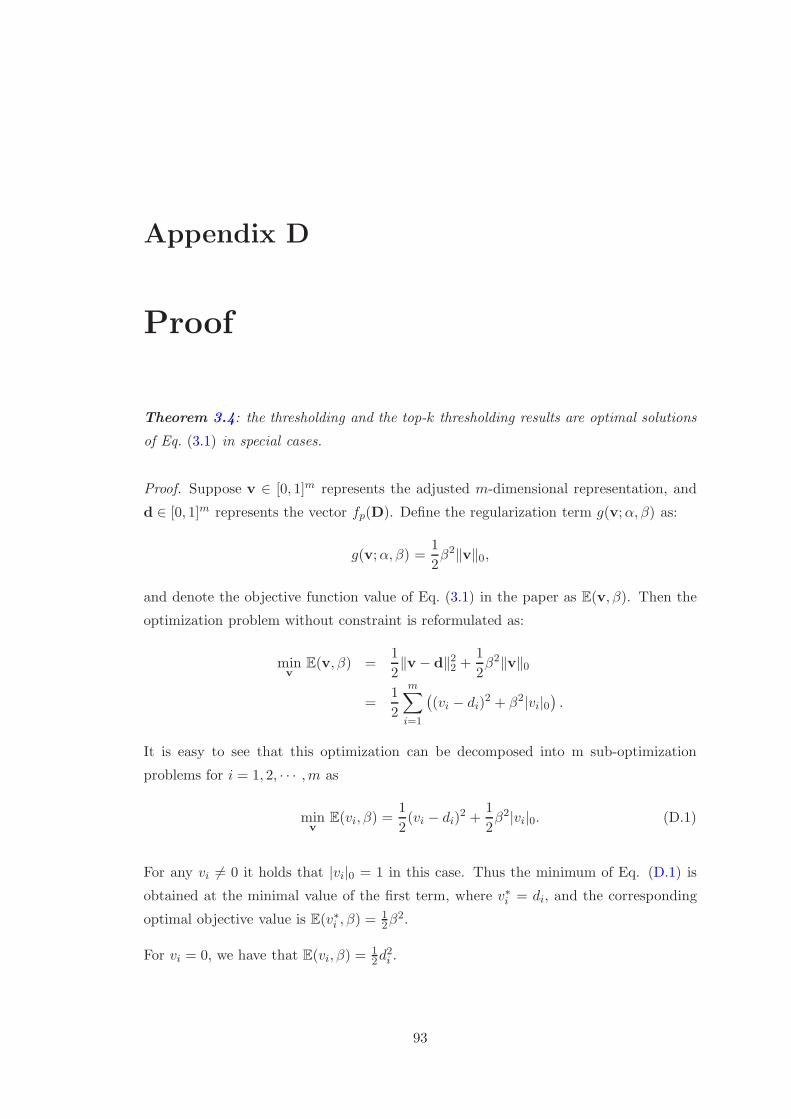
Appendix D
Proof
Theorem 3.4: the thresholding and the top-k thresholding results are optimal solutions
of Eq. (3.1) in special cases.
Proof. Suppose v ∈ [0, 1]m represents the adjusted m-dimensional representation, and
d ∈ [0, 1]m represents the vector fp(D). Define the regularization term g(v;α, β) as:
g(v;α, β) =1
2β2‖v‖0,
and denote the objective function value of Eq. (3.1) in the paper as E(v, β). Then the
optimization problem without constraint is reformulated as:
minv
E(v, β) =1
2‖v − d‖22 +
1
2β2‖v‖0
=1
2
m∑
i=1
((vi − di)
2 + β2|vi|0).
It is easy to see that this optimization can be decomposed into m sub-optimization
problems for i = 1, 2, · · · ,m as
minv
E(vi, β) =1
2(vi − di)
2 +1
2β2|vi|0. (D.1)
For any vi 6= 0 it holds that |vi|0 = 1 in this case. Thus the minimum of Eq. (D.1) is
obtained at the minimal value of the first term, where v∗i = di, and the corresponding
optimal objective value is E(v∗i , β) =12β
2.
For vi = 0, we have that E(vi, β) =12d
2i .
93
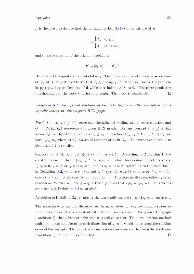
Appendix 94
It is then easy to deduce that the optimum of Eq. (D.1) can be calculated at:
v∗i =
di, di ≥ β
0, otherwise,
and thus the solution of the original problem is
v∗ = [v∗1 , v∗2 , · · · , v∗m]T .
Denote the kth largest component of d is dk. Then if we want to get the k-sparse solution
of Eq. (3.1), we just need to set that dk ≤ β < dk+1. Then the solution of the problem
keeps top-k largest elements of d while thresholds others to 0. This corresponds the
thresholding and the top-k thresholding results. The proof is completed.
Theorem 3.3: the optimal solutions of Eq. (3.1) (before or after normalization) is
logically consistent with its given HEX graph.
Proof. Suppose v ∈ [0, 1]m represents the adjusted m-dimensional representation, and
G = (N,Eh, Ee) represents the given HEX graph. For any concept (ni, nj) ∈ Eh,
according to Algorithm 1, we have vi ≥ vj . Therefore ∀nk, nj ∈ V , nk ∈ α(nj), we
have vk ≥ vj , where α(nj) is a set of ancestor of nj in Gh . This means condition 1 in
Definition 3.2 is satisfied.
Suppose ∃np ∈ α(ni), ∃nq ∈ α(nj) s.t. (np, nq) ∈ Ee. According to Algorithm 1, the
constraints ensure that if (np, nq) ∈ Eh, vpvq = 0, which breaks down into three cases:
1) vp 6= 0, vq = 0, 2) vp = 0, vq 6= 0, and 3) vp = vq = 0. According to the condition 1
in Definition 3.2, we have vp ≥ vi and vq ≥ vj so for case 1) we have vj ≤ vq = 0; for
case 2) vi ≤ vp = 0; for case 3) vi = 0 and vj = 0. Therefore in all cases, either vi or vj
is nonzero. When i = p and j = q, it trivially holds that vpvq = vivj = 0. This means
condition 2 in Definition 3.2 is satisfied.
According to Definition 3.2, v satisfies the two conditions and thus is logically consistent.
The normalization method discussed in the paper does not change nonzero scores to
zero or vice versa. If v is consistent with the exclusion relation in the given HEX graph
(condition 2), then after normalization it is still consistent. The normalization method
multiples a constant factor to each dimension of v so it would not change the ranking
order of the concepts. Therefore the normalization also preserves the hierarchical relation
(condition 1). The proof is completed.
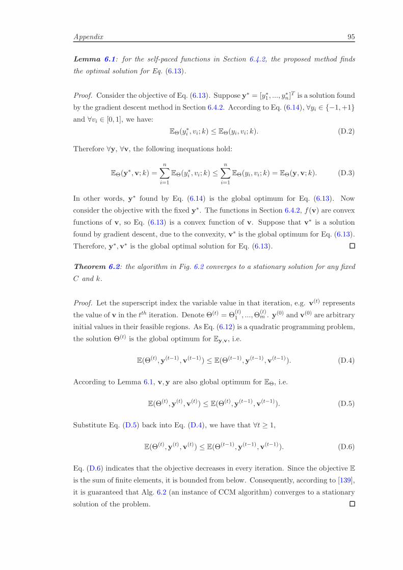
Appendix 95
Lemma 6.1: for the self-paced functions in Section 6.4.2, the proposed method finds
the optimal solution for Eq. (6.13).
Proof. Consider the objective of Eq. (6.13). Suppose y∗ = [y∗1 , ..., y∗n]
T is a solution found
by the gradient descent method in Section 6.4.2. According to Eq. (6.14), ∀yi ∈ −1,+1and ∀vi ∈ [0, 1], we have:
EΘ(y∗i , vi; k) ≤ EΘ(yi, vi; k). (D.2)
Therefore ∀y, ∀v, the following inequations hold:
EΘ(y∗,v; k) =
n∑
i=1
EΘ(y∗i , vi; k) ≤
n∑
i=1
EΘ(yi, vi; k) = EΘ(y,v; k). (D.3)
In other words, y∗ found by Eq. (6.14) is the global optimum for Eq. (6.13). Now
consider the objective with the fixed y∗. The functions in Section 6.4.2, f(v) are convex
functions of v, so Eq. (6.13) is a convex function of v. Suppose that v∗ is a solution
found by gradient descent, due to the convexity, v∗ is the global optimum for Eq. (6.13).
Therefore, y∗,v∗ is the global optimal solution for Eq. (6.13).
Theorem 6.2: the algorithm in Fig. 6.2 converges to a stationary solution for any fixed
C and k.
Proof. Let the superscript index the variable value in that iteration, e.g. v(t) represents
the value of v in the tth iteration. Denote Θ(t) = Θ(t)1 , ...,Θ
(t)m . y(0) and v(0) are arbitrary
initial values in their feasible regions. As Eq. (6.12) is a quadratic programming problem,
the solution Θ(t) is the global optimum for Ey,v, i.e.
E(Θ(t),y(t−1),v(t−1)) ≤ E(Θ(t−1),y(t−1),v(t−1)). (D.4)
According to Lemma 6.1, v,y are also global optimum for EΘ, i.e.
E(Θ(t),y(t),v(t)) ≤ E(Θ(t),y(t−1),v(t−1)). (D.5)
Substitute Eq. (D.5) back into Eq. (D.4), we have that ∀t ≥ 1,
E(Θ(t),y(t),v(t)) ≤ E(Θ(t−1),y(t−1),v(t−1)). (D.6)
Eq. (D.6) indicates that the objective decreases in every iteration. Since the objective E
is the sum of finite elements, it is bounded from below. Consequently, according to [139],
it is guaranteed that Alg. 6.2 (an instance of CCM algorithm) converges to a stationary
solution of the problem.

Appendix 96
Theorem 7.4: For training samples X = xini=1, given a curriculum γ defined on it,
the feasible region, defined by,
Ψ = v|aTv ≤ c (D.7)
is a curriculum region of γ if it holds: 1) Ψ ∧ v ∈ [0, 1]n is nonempty; 2) ai<aj for all
γ(xi)<γ(xj); ai=aj for all γ(xi)=γ(xj).
Proof. (1) Ψ ∧ v ∈ [0, 1]n is a nonempty convex set.
(2) For xi,xj with γ(xi) < γ(xj), denote Ψij = vij |aTijvij≤c, aij/vij the sub-vector
of a/v by wiping off its ith and jth elements, respectively, we can then calculate the
expected value of vi on the region Ψ = v|aTv ≤c as:
E(vi) =
∫
Ψvi dv
=
∫
Ψij
∫ c−aTijvij
aj
0
∫ c−aTijvij−ajvj
ai
0vidvidvjdvij
=
∫
Ψij
∫ c−aTijvij
aj
0
(c− aTijvij − ajvj
)2
2a2idvjdvij
=
∫Ψij
(c− aTijvij
)3dvij
6a2i aj.
In the similar way, we can get that:
E(vj) =
∫
Ψvj dv =
∫Ψij
(c− aTijvij
)3dvij
6a2jai.
We thus can get that
E(vi)− E(vj) =
∫Ψij
(c− aTijvij
)3dvij
6a2i a2j
(aj − ai) > 0.
Similarly, we can prove that∫Ψ vi dΨ =
∫Ψ vj dΨ for γ(xi) = γ(xj).
The proof is then completed.
Theorem 7.5: The binary, linear, logarithmic and mixture scheme are self-paced func-
tions.
Proof. We first prove the above functions satisfying Condition 1 in Definition 7.3, i.e.
they are convex with respect to v ∈ [0, 1]n, where n is the number of samples. As

Appendix 97
binary, linear, logarithmic and mixture self-paced functions can be decoupled f(v;λ) =∑n
i=1 f(vi;λ):
For binary scheme f(vi;λ) = −λvi:
∂2f
∂2vi= 0. (D.8)
For linear scheme f(vi;λ) =12λ(v
2i − 2vi):
∂2f
∂2vi= λ > 0, (D.9)
where λ > 0.
For logarithmic scheme f(vi;λ) = ζvi − ζvi
log ζ :
∂2f
∂2vi= − 1
log ζζvi > 0, (D.10)
where ζ = 1− λ and λ ∈ (0, 1).
For mixture scheme f(vi;λ) = −ζ log(vi + 1λ1ζ):
∂2f
∂2vi=
ζλ21
(ζ + λ1vi)2> 0 (D.11)
where λ = [λ1, λ2], ζ = λ1λ2λ1−λ2
, and λ1 > λ2 > 0.
As the above second derivatives are non-negative, and the sum of convex functions is
convex, we have f(v;λ) for binary, linear, logarithmic and mixture scheme are convex.
We then prove the above functions satisfying Condition 2 that is when all variables are
fixed except for vi, ℓi, v∗i decreases with ℓi
Denote Ew =∑n
i=1 viℓi + f(v;λ) as the objective with the fixed model parameters w,
where ℓi is the loss for the ith sample. The optimal solution v∗ = [v∗1 , · · · , v∗n]T =
argminv∈[0,1]n Ew.

Appendix 98
For binary scheme:
Ew =n∑
i=1
(ℓi − λ)vi;
∂Ew
∂vi= ℓi − λ = 0;
⇒ v∗i =
1 ℓi < λ
0 ℓi ≥ λ.
(D.12)
For linear scheme:
Ew =
n∑
i=1
ℓivi +1
2λ(v2i − 2vi);
∂Ew
∂vi= ℓ+ viλ− λ = 0;
⇒ v∗i =
− 1
λℓ+ 1 ℓi < λ
0 ℓi ≥ λ.
(D.13)
For logarithmic scheme:
Ew =
n∑
i=1
ℓivi + ζvi −ζvi
log ζ;
∂Ew
∂vi= ℓ+ ζ − ζvi = 0;
⇒ v∗i =
1log ζ log(ℓ+ ζ) ℓi < λ
0 ℓi ≥ λ.
(D.14)
where ζ = 1− λ (0 < λ < 1).
For mixture scheme:
Ew =
n∑
i=1
ℓivi − ζ log(vi +1
λ1ζ);
∂Ew
∂vi= ℓ− ζλ1
ζ + λ1vi= 0;
⇒ v∗i =
1 ℓi ≤ λ2
0 ℓi ≥ λ1
(λ1−ℓ)ζℓλ1
λ2 < ℓi < λ1
(D.15)
where λ = [λ1, λ2], and ζ = λ1λ2λ1−λ2
, (λ1 > λ2 > 0).

Appendix 99
By setting the partial gradient to zero we arrive the optimal solution of v. It is obvious
that vi is decreasing with respect to ℓi in all functions. In all cases, we have that
limℓi→0
v∗i = 1, limℓi→∞
v∗i = 0.
Finally, we prove that the above functions satisfying Condition 3 that is ‖v‖1 increases
with respect to λ, and it holds that ∀i∈ [1, n], limλ→0
v∗i =0, limλ→∞
v∗i =1.
It is easy to verify that each individual v∗i increases with respect to λ in their closed-form
solutions in Eq. (D.12), Eq. (D.13), Eq. (D.14) and Eq. (D.15) (in mixture scheme, let
λ = λ1 represent the model age). Therefore ‖v‖1 =∑n
i=1 vi also increases with respect
to λ. In an extreme case, when λ approaches positive infinity, we have ∀i ∈ [1, n]vi = 1,
i.e. limλ→∞
v∗i =1 in Eq. (D.12), Eq. (D.13), Eq. (D.14) and Eq. (D.15). Similarly, when
λ approaches 0, we have limλ→0
v∗i =0.
As binary, linear, logarithmic and mixture scheme satisfy the three conditions, they are
all self-paced functions.
The proof is then completed.
Theorem 7.6: Algorithm 3 attains the global optimum to minv E(w,v) for any given
w in linearithmic time.
Proof. Given the training dataset D = (x1, y1), · · · , (xn, yn), where xi ∈ Rm denotes
the ith observed sample and yi denotes its label. Assume that the training samples
X = [x1, · · · ,xn] are with b groups: X(1), · · · ,X(b), where X(j) = (x(j)1 , · · · ,x(j)
nj ) ∈Rm×nj corresponds to samples in the jth group, nj is the sample number in this group
and∑b
j=1 nj = n. Accordingly, denote the weight vector as v = [v(1), · · · ,v(b)], where
v(j) = (v(j)1 , · · · , v(j)nj )
T ∈ Rnj . The following theorem proves that Algorithm 1 can get
the global solution of the following non-convex optimization problem:
minv∈[0,1]n
E(w,v;λ, γ) =
n∑
i=1
viL(yi, f(xi,w))− λ
n∑
i=1
vi − γ‖v‖2,1, (D.16)
where L(yi, f(xi,w)) denotes the loss function which calculates the cost between the
ground truth label yi and the estimated label f(xi,w), and the l2,1-norm ‖v‖2,1 is the
group sparsity of v:
‖v‖2,1 =b∑
j=1
‖v(j)‖2.
For convenience we briefly rewrite E(w,v;λ, γ) and L(yi, f(xi,w)) as E(v) and Li,
respectively.

Appendix 100
The weight vector v∗ outputted from Algorithm 1 attains the global optimal solution of
the optimization problem (D.16), i.e.,
v∗ = arg minv∈[0,1]n
E(v).
The objective function of (D.16) can be reformulated as the following decoupling forms
based on the data cluster information:
E(v) =b∑
j=1
E(v(j)), (D.17)
where
E(v(j)) =
nj∑
i=1
v(j)i L
(j)i − λ
nj∑
i=1
v(j)i − γ‖v(j)‖2, (D.18)
where L(j)i represents the loss value of x
(j)i . It is easy to see that the original problem
(D.16) can be equivalently decomposed as a series of the following sub-optimization
problems (j = 1, · · · , b):v(j)∗ = arg min
v(j)∈[0,1]njE(v(j)). (D.19)
E(v(j)) defined in Eq. (D.18) is a concave function since its first and second terms are
linear, and the third term is the negative l2,1 norm, whose positive form is a commonly
utilized convex regularizer. It is well known that the minimum solution of a concave
function over a polytope can be obtained at its vertices [140]. In other words, for the
optimization problem (D.19), it holds that its optimal solution v(j)∗ ∈ 0, 1nj , i.e.,
v(j)∗ = arg minv(j)∈0,1nj
E(v(j)). (D.20)
For k = 1, · · · , nj, let’s denote
v(j)(k) = arg min
v(j) ∈ 0, 1nj
‖v(j)‖0 = k
E(v(j)). (D.21)
This means that v(j)(k) is the optimum of (D.19) if it is further constrained to be with
k nonzero entries. It is then easy to deduce that
v(j)∗ = arg minv(j)(k)
E(v(j)(k)). (D.22)

Appendix 101
That is, the optimal solution v(j)∗ of (D.19) can be achieved among v(j)(1), · · · ,v(j)(nj)
at which the minimal objective value is attained.
Without loss of generality, we assume that the samples (x(j)1 , · · · ,x(j)
nj ) in the jth cluster
are arranged in the ascending order of their loss values L(j)i . Then for the optimization
problem (D.21), we can get that
min
v(j) ∈ 0, 1nj
‖v(j)‖0 = k
E(v(j)) =
nj∑
i=1
v(j)i L
(j)i − λ
nj∑
i=1
v(j)i − γ‖v(j)‖2
⇔ min
v(j) ∈ 0, 1nj
‖v(j)‖0 = k
nj∑
i=1
v(j)i L
(j)i ,
since the last two terms in E(v(j)) are with constant values under the constraint. Then
it is easy to get that the optimal solution v(j)(k) of (D.21) is attained by setting its k
entries corresponding to the k smallest loss values L(j)i (i.e., the first k entries of v(j)(k))
as 1 while others as 0, and the minimal objective value is
E(v(j)(k)) =k∑
i=1
v(j)i L
(j)i − λk − γ
√k. (D.23)
Then let’s calculate the difference between any two adjacent elements in the sequence
E(v(j)(1)), · · · , E(v(j)(nj)):
diffk = E(v(j)(k + 1))− E(v(j)(k))
= L(j)k+1 − λ− γ(
√k + 1−
√k)
= L(j)k+1 − (λ+ γ
1√k + 1 +
√k).
Since L(j)k (with respect to k) is a monotonically increasing sequence while λ+γ 1√
k+1+√k
is a monotonically decreasing sequence, diffk is a monotonically increasing sequence.
Denote k∗ as the index where its first positive value is attained (if diffk ≤ 0 for all
k = 1, · · · , nj − 1, k∗ = nj). Then it is easy to get that E(v(j)(k)) is monotonically
decreasing until k = k∗ and then it starts to be monotonically increasing. This means
that E(v(j)(k∗)) gets the minimum among all E(v(j)(1)), · · · , E(v(j)(nj)). Based on
(D.22), we know that the global optimum v(j)∗ of (D.19) is attained at v(j)(k∗).
By independently calculating the optimum v(j)∗ for each cluster and then combining
them, the global optimal solution v∗ of (D.16) can then be calculated. This corresponds

Appendix 102
to the process of our proposed Algorithm 3.
The most computational complex step in the above derivation is the sort of nj (1 ≤ j ≤ b)
samples. Since nj < n, the average-case complexity is thus upper bounded by O(n log n),
assuming that the quick sort algorithm is used.
The proof is completed.

Appendix E
Detailed Results
Table E.1: Event-level comparison of AP on the 10 splits of MED13Test.
Event ID & Name Raw + Expert Adjusted + Expert Adjusted + Auto Adjusted + AutoVisualE006: Birthday party 0.3411 0.2980 0.1207 0.1207E007: Changing a vehicle tire 0.0967 0.1667 0.2061 0.0134E008: Flash mob gathering 0.2087 0.1647 0.1028 0.1028E009: Getting a vehicle unstuck 0.1416 0.1393 0.0569 0.0569E010: Grooming an animal 0.0442 0.0479 0.0128 0.0128E011: Making a sandwich 0.0909 0.0804 0.2910 0.0709E012: Parade 0.4552 0.4685 0.2027 0.2027E013: Parkour 0.0498 0.0596 0.0619 0.0525E014: Repairing an appliance 0.2731 0.2376 0.2262 0.0234E015: Working on a sewing project 0.2022 0.2184 0.0135 0.0045E021: Attempting a bike trick 0.0969 0.1163 0.0486 0.0486E022: Cleaning an appliance 0.1248 0.1248 0.1248 0.0124E023: Dog show 0.7284 0.7288 0.6028 0.6027E024: Giving directions to a location 0.0253 0.0252 0.0252 0.0069E025: Marriage proposal 0.0748 0.0750 0.0755 0.0011E026: Renovating a home 0.0139 0.0061 0.0049 0.0049E027: Rock climbing 0.1845 0.1724 0.0668 0.0668E028: Town hall meeting 0.1585 0.0898 0.0163 0.0163E029: Winning a race without a vehicle 0.1470 0.1697 0.0584 0.0584E030: Working on a metal crafts project 0.0673 0.0422 0.0881 0.0026MAP 0.1762 0.1716 0.1203 0.0741
103

Appendix 104
Table E.2: Event-level comparison of AP on the 10 splits of MED14Test.
Event ID & Name Raw + Expert Adjusted + Expert Adjusted + Auto Adjusted + AutoVisualE021: Attempting a bike trick 0.0632 0.0678 0.0814 0.0822E022: Cleaning an appliance 0.2634 0.2635 0.2634 0.2636E023: Dog show 0.6757 0.6449 0.4387 0.4414E024: Giving directions to a location 0.0613 0.0613 0.0614 0.0612E025: Marriage proposal 0.0176 0.0174 0.0181 0.0174E026: Renovating a home 0.0252 0.0089 0.0043 0.0043E027: Rock climbing 0.2082 0.1302 0.0560 0.0560E028: Town hall meeting 0.2478 0.0925 0.0161 0.0161E029: Winning a race without a vehicle 0.1234 0.1848 0.0493 0.0497E030: Working on a metal crafts project 0.1238 0.0616 0.0981 0.0981E031: Beekeeping 0.5900 0.5221 0.4217 0.4258E032: Wedding shower 0.0834 0.0924 0.0922 0.0395E033: Non-motorized vehicle repair 0.5218 0.4525 0.0149 0.0150E034: Fixing musical instrument 0.0284 0.0439 0.0439 0.0023E035: Horse riding competition 0.3673 0.3346 0.0994 0.0993E036: Felling a tree 0.0970 0.0620 0.0108 0.0108E037: Parking a vehicle 0.2921 0.2046 0.0313 0.0313E038: Playing fetch 0.0339 0.0284 0.0016 0.0014E039: Tailgating 0.1429 0.0200 0.0010 0.0010E040: Tuning musical instrument 0.1553 0.1553 0.1840 0.0128MAP 0.2061 0.1724 0.0994 0.0865
Table E.3: Performance for 30 commercials on the YFCC100 set.
ID Query Name Commercial ProductEvaluation Metric
CategoryP@20 MRR MAP@20
1 football and running soccer shoes 0.80 1.00 0.88 Sport2 auto racing sport cars 0.70 1.00 0.91 Auto3 dog show dog training collars 0.95 1.00 0.97 Grocery4 baby stroller/diapper 1.00 1.00 1.00 Grocery5 fire burning smoke fire prevention 0.95 1.00 0.96 Miscellaneous6 cake or birthday cake birthday cake 0.35 0.50 0.60 Grocery7 underwater diving 1.00 1.00 1.00 Sports8 dog indoor dog food 0.75 1.00 0.67 Grocery9 riding horse horse riding lessons 0.90 1.00 0.93 Sports10 kitchen food restaurant 1.00 1.00 1.00 Grocery11 Christmas decoration decoration 0.80 1.00 0.87 Grocery12 dancing dancing lessons 0.90 1.00 0.90 Miscellaneous13 bicycling cycling cloth and helmet 0.95 1.00 0.99 Sports14 car and vehicle car tires 1.00 1.00 1.00 Auto15 skiing or snowboarding ski resort 0.95 1.00 0.96 Sports16 parade flags or banners 0.90 1.00 0.96 Grocery17 music band live music show 1.00 1.00 1.00 Grocery18 busking live show 0.20 1.00 0.50 Miscellaneous19 home renovation furniture 0.00 0.00 0.00 Miscellaneous20 speaking in front of people speaking in public training 0.65 0.50 0.63 Miscellaneous21 sunny beach vacation by beach 1.00 1.00 1.00 Traveling22 politicians vote Obama 0.60 1.00 0.63 Miscellaneous23 female face makeup 1.00 1.00 1.00 Miscellaneous24 cell phone cell phone 0.80 1.00 0.96 Miscellaneous25 fireworks fireworks 0.95 1.00 0.96 Miscellaneous26 tennis tennis 1.00 1.00 1.00 Sports27 helicopter helicopter tour 1.00 1.00 1.00 Traveling28 cooking pan 0.90 1.00 0.92 Miscellaneous29 eiffel night hotels in Paris 0.90 1.00 0.89 Traveling30 table tennis ping pong 0.60 1.00 0.85 Sports
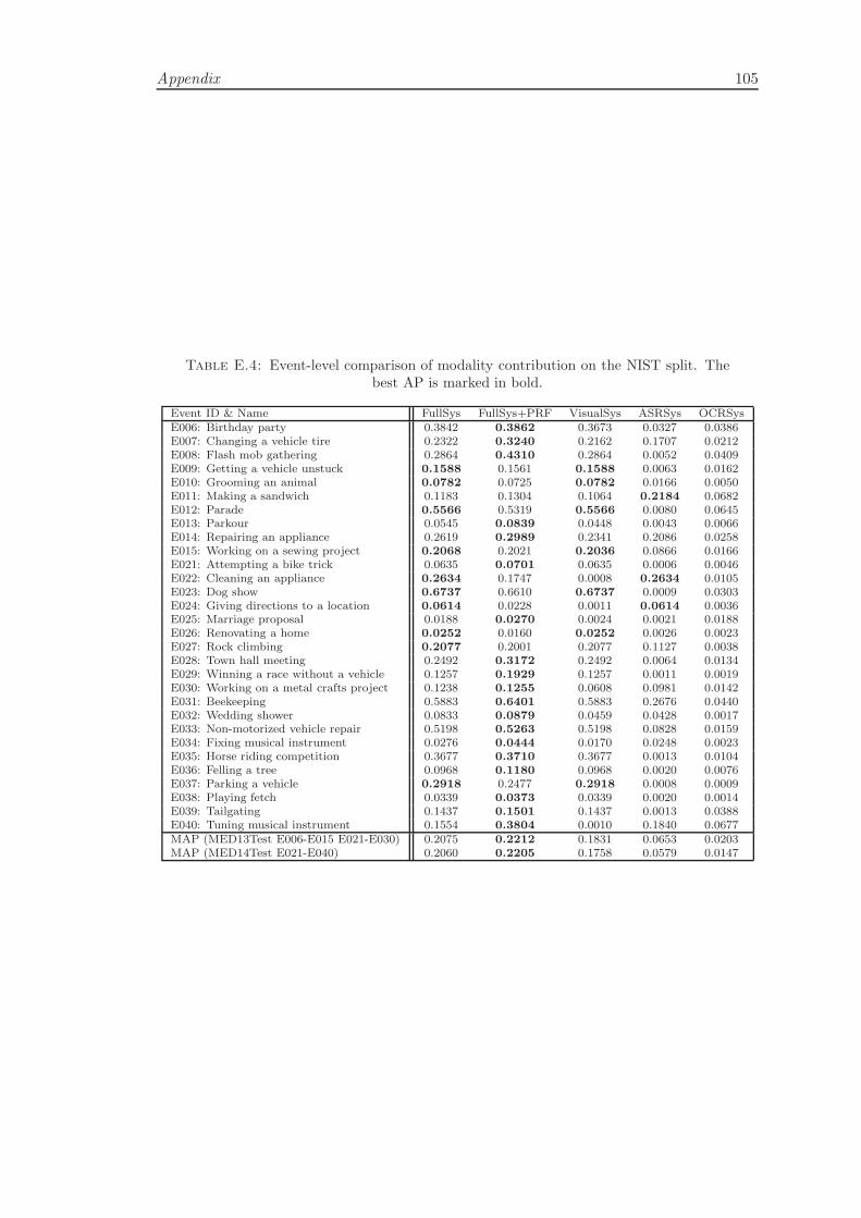
Appendix 105
Table E.4: Event-level comparison of modality contribution on the NIST split. Thebest AP is marked in bold.
Event ID & Name FullSys FullSys+PRF VisualSys ASRSys OCRSysE006: Birthday party 0.3842 0.3862 0.3673 0.0327 0.0386E007: Changing a vehicle tire 0.2322 0.3240 0.2162 0.1707 0.0212E008: Flash mob gathering 0.2864 0.4310 0.2864 0.0052 0.0409E009: Getting a vehicle unstuck 0.1588 0.1561 0.1588 0.0063 0.0162E010: Grooming an animal 0.0782 0.0725 0.0782 0.0166 0.0050E011: Making a sandwich 0.1183 0.1304 0.1064 0.2184 0.0682E012: Parade 0.5566 0.5319 0.5566 0.0080 0.0645E013: Parkour 0.0545 0.0839 0.0448 0.0043 0.0066E014: Repairing an appliance 0.2619 0.2989 0.2341 0.2086 0.0258E015: Working on a sewing project 0.2068 0.2021 0.2036 0.0866 0.0166E021: Attempting a bike trick 0.0635 0.0701 0.0635 0.0006 0.0046E022: Cleaning an appliance 0.2634 0.1747 0.0008 0.2634 0.0105E023: Dog show 0.6737 0.6610 0.6737 0.0009 0.0303E024: Giving directions to a location 0.0614 0.0228 0.0011 0.0614 0.0036E025: Marriage proposal 0.0188 0.0270 0.0024 0.0021 0.0188E026: Renovating a home 0.0252 0.0160 0.0252 0.0026 0.0023E027: Rock climbing 0.2077 0.2001 0.2077 0.1127 0.0038E028: Town hall meeting 0.2492 0.3172 0.2492 0.0064 0.0134E029: Winning a race without a vehicle 0.1257 0.1929 0.1257 0.0011 0.0019E030: Working on a metal crafts project 0.1238 0.1255 0.0608 0.0981 0.0142E031: Beekeeping 0.5883 0.6401 0.5883 0.2676 0.0440E032: Wedding shower 0.0833 0.0879 0.0459 0.0428 0.0017E033: Non-motorized vehicle repair 0.5198 0.5263 0.5198 0.0828 0.0159E034: Fixing musical instrument 0.0276 0.0444 0.0170 0.0248 0.0023E035: Horse riding competition 0.3677 0.3710 0.3677 0.0013 0.0104E036: Felling a tree 0.0968 0.1180 0.0968 0.0020 0.0076E037: Parking a vehicle 0.2918 0.2477 0.2918 0.0008 0.0009E038: Playing fetch 0.0339 0.0373 0.0339 0.0020 0.0014E039: Tailgating 0.1437 0.1501 0.1437 0.0013 0.0388E040: Tuning musical instrument 0.1554 0.3804 0.0010 0.1840 0.0677MAP (MED13Test E006-E015 E021-E030) 0.2075 0.2212 0.1831 0.0653 0.0203MAP (MED14Test E021-E040) 0.2060 0.2205 0.1758 0.0579 0.0147
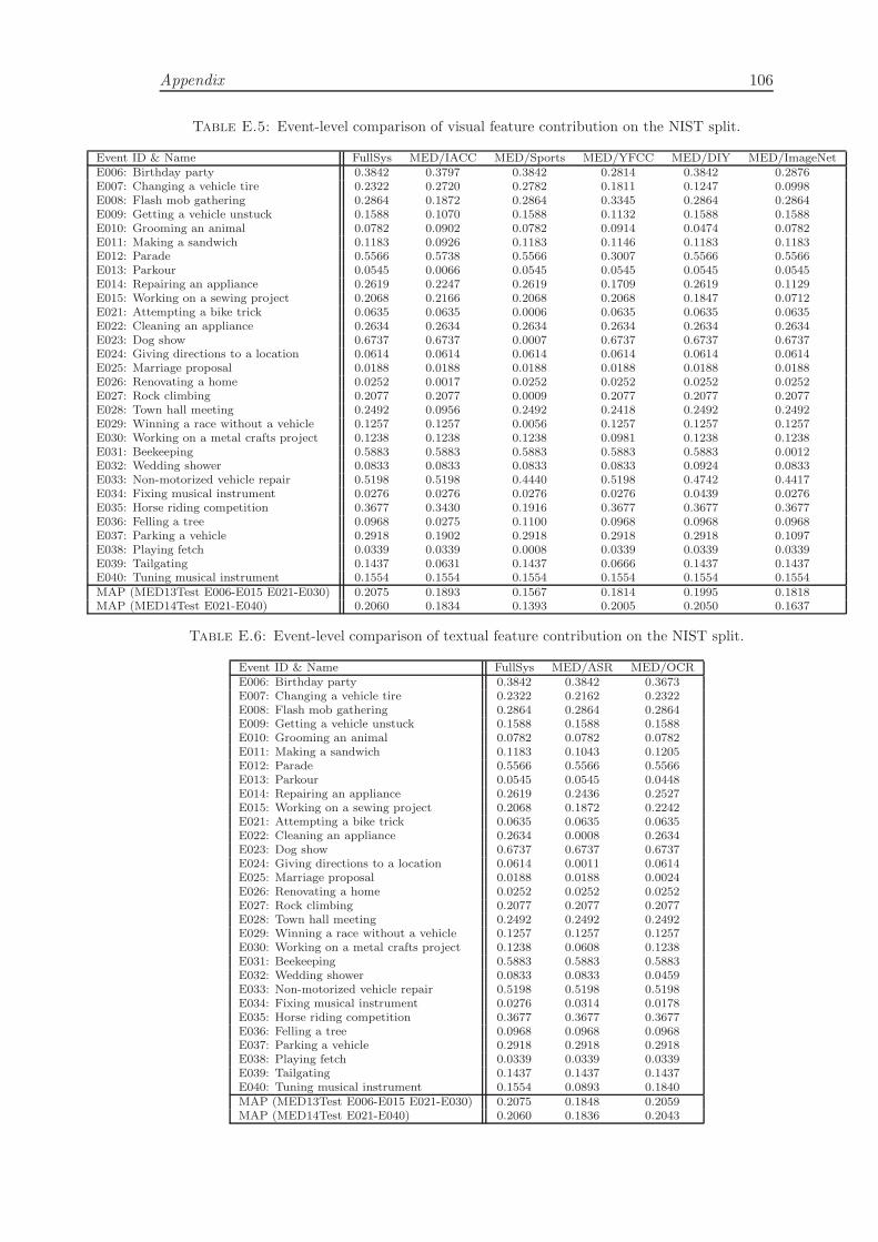
Appendix 106
Table E.5: Event-level comparison of visual feature contribution on the NIST split.
Event ID & Name FullSys MED/IACC MED/Sports MED/YFCC MED/DIY MED/ImageNetE006: Birthday party 0.3842 0.3797 0.3842 0.2814 0.3842 0.2876E007: Changing a vehicle tire 0.2322 0.2720 0.2782 0.1811 0.1247 0.0998E008: Flash mob gathering 0.2864 0.1872 0.2864 0.3345 0.2864 0.2864E009: Getting a vehicle unstuck 0.1588 0.1070 0.1588 0.1132 0.1588 0.1588E010: Grooming an animal 0.0782 0.0902 0.0782 0.0914 0.0474 0.0782E011: Making a sandwich 0.1183 0.0926 0.1183 0.1146 0.1183 0.1183E012: Parade 0.5566 0.5738 0.5566 0.3007 0.5566 0.5566E013: Parkour 0.0545 0.0066 0.0545 0.0545 0.0545 0.0545E014: Repairing an appliance 0.2619 0.2247 0.2619 0.1709 0.2619 0.1129E015: Working on a sewing project 0.2068 0.2166 0.2068 0.2068 0.1847 0.0712E021: Attempting a bike trick 0.0635 0.0635 0.0006 0.0635 0.0635 0.0635E022: Cleaning an appliance 0.2634 0.2634 0.2634 0.2634 0.2634 0.2634E023: Dog show 0.6737 0.6737 0.0007 0.6737 0.6737 0.6737E024: Giving directions to a location 0.0614 0.0614 0.0614 0.0614 0.0614 0.0614E025: Marriage proposal 0.0188 0.0188 0.0188 0.0188 0.0188 0.0188E026: Renovating a home 0.0252 0.0017 0.0252 0.0252 0.0252 0.0252E027: Rock climbing 0.2077 0.2077 0.0009 0.2077 0.2077 0.2077E028: Town hall meeting 0.2492 0.0956 0.2492 0.2418 0.2492 0.2492E029: Winning a race without a vehicle 0.1257 0.1257 0.0056 0.1257 0.1257 0.1257E030: Working on a metal crafts project 0.1238 0.1238 0.1238 0.0981 0.1238 0.1238E031: Beekeeping 0.5883 0.5883 0.5883 0.5883 0.5883 0.0012E032: Wedding shower 0.0833 0.0833 0.0833 0.0833 0.0924 0.0833E033: Non-motorized vehicle repair 0.5198 0.5198 0.4440 0.5198 0.4742 0.4417E034: Fixing musical instrument 0.0276 0.0276 0.0276 0.0276 0.0439 0.0276E035: Horse riding competition 0.3677 0.3430 0.1916 0.3677 0.3677 0.3677E036: Felling a tree 0.0968 0.0275 0.1100 0.0968 0.0968 0.0968E037: Parking a vehicle 0.2918 0.1902 0.2918 0.2918 0.2918 0.1097E038: Playing fetch 0.0339 0.0339 0.0008 0.0339 0.0339 0.0339E039: Tailgating 0.1437 0.0631 0.1437 0.0666 0.1437 0.1437E040: Tuning musical instrument 0.1554 0.1554 0.1554 0.1554 0.1554 0.1554MAP (MED13Test E006-E015 E021-E030) 0.2075 0.1893 0.1567 0.1814 0.1995 0.1818MAP (MED14Test E021-E040) 0.2060 0.1834 0.1393 0.2005 0.2050 0.1637
Table E.6: Event-level comparison of textual feature contribution on the NIST split.
Event ID & Name FullSys MED/ASR MED/OCRE006: Birthday party 0.3842 0.3842 0.3673E007: Changing a vehicle tire 0.2322 0.2162 0.2322E008: Flash mob gathering 0.2864 0.2864 0.2864E009: Getting a vehicle unstuck 0.1588 0.1588 0.1588E010: Grooming an animal 0.0782 0.0782 0.0782E011: Making a sandwich 0.1183 0.1043 0.1205E012: Parade 0.5566 0.5566 0.5566E013: Parkour 0.0545 0.0545 0.0448E014: Repairing an appliance 0.2619 0.2436 0.2527E015: Working on a sewing project 0.2068 0.1872 0.2242E021: Attempting a bike trick 0.0635 0.0635 0.0635E022: Cleaning an appliance 0.2634 0.0008 0.2634E023: Dog show 0.6737 0.6737 0.6737E024: Giving directions to a location 0.0614 0.0011 0.0614E025: Marriage proposal 0.0188 0.0188 0.0024E026: Renovating a home 0.0252 0.0252 0.0252E027: Rock climbing 0.2077 0.2077 0.2077E028: Town hall meeting 0.2492 0.2492 0.2492E029: Winning a race without a vehicle 0.1257 0.1257 0.1257E030: Working on a metal crafts project 0.1238 0.0608 0.1238E031: Beekeeping 0.5883 0.5883 0.5883E032: Wedding shower 0.0833 0.0833 0.0459E033: Non-motorized vehicle repair 0.5198 0.5198 0.5198E034: Fixing musical instrument 0.0276 0.0314 0.0178E035: Horse riding competition 0.3677 0.3677 0.3677E036: Felling a tree 0.0968 0.0968 0.0968E037: Parking a vehicle 0.2918 0.2918 0.2918E038: Playing fetch 0.0339 0.0339 0.0339E039: Tailgating 0.1437 0.1437 0.1437E040: Tuning musical instrument 0.1554 0.0893 0.1840MAP (MED13Test E006-E015 E021-E030) 0.2075 0.1848 0.2059MAP (MED14Test E021-E040) 0.2060 0.1836 0.2043

Bibliography
[1] John R Smith. Riding the multimedia big data wave. In SIGIR, 2013.
[2] James Davidson, Benjamin Liebald, Junning Liu, et al. The youtube video rec-
ommendation system. In RecSys, 2010.
[3] Baptist Vandersmissen, Frederic Godin, Abhineshwar Tomar, Wesley De Neve,
and Rik Van de Walle. The rise of mobile and social short-form video: an in-
depth measurement study of vine. In ICMR Workshop on Social Multimedia and
Storytelling, 2014.
[4] Paul Over, George Awad, Martial Michel, Jonathan Fiscus, Greg Sanders, Wessel
Kraaij, Alan F. Smeaton, and Georges Quenot. TRECVID 2014 – an overview of
the goals, tasks, data, evaluation mechanisms and metrics. In NIST TRECVID,
2014.
[5] Shicheng Xu, Huan Li, Xiaojun Chang, Shoou-I Yu, Xingzhong Du, Xuanchong
Li, Lu Jiang, Zexi Mao, Zhenzhong Lan, Susanne Burger, et al. Incremental
multimodal query construction for video search. In ICMR, 2015.
[6] Fiona Fui-Hoon Nah. A study on tolerable waiting time: how long are web users
willing to wait? Behaviour & Information Technology, 23(3):153–163, 2004.
[7] Meng Wang, Richang Hong, Guangda Li, Zheng-Jun Zha, Shuicheng Yan, and
Tat-Seng Chua. Event driven web video summarization by tag localization and
key-shot identification. Multimedia, IEEE Transactions on, 14(4):975–985, 2012.
[8] Evlampios Apostolidis, Vasileios Mezaris, Mathilde Sahuguet, Benoit Huet, Barbo-
ra Cervenkova, Daniel Stein, Stefan Eickeler, Jose Luis Redondo Garcia, Raphael
Troncy, and Lukas Pikora. Automatic fine-grained hyperlinking of videos within
a closed collection using scene segmentation. In MM, 2014.
[9] Yue Gao, Sicheng Zhao, Yang Yang, and Tat-Seng Chua. Multimedia social event
detection in microblog. In MMM, 2015.
107

Bibliography 108
[10] Lu Jiang, Shoou-I Yu, Deyu Meng, Yi Yang, Teruko Mitamura, and Alexander G
Hauptmann. Fast and accurate content-based semantic search in 100m internet
videos. In MM, 2015.
[11] Fabricio Benevenuto, Tiago Rodrigues, Virgılio AF Almeida, Jussara Almeida,
Marcos Goncalves, and Keith Ross. Video pollution on the web. First Monday,
15(4), 2010.
[12] Zhuo Chen, Lu Jiang, Wenlu Hu, Kiryong Ha, Brandon Amos, Padmanabhan
Pillai, Alex Hauptmann, and Mahadev Satyanarayanan. Early implementation
experience with wearable cognitive assistance applications. In WEARSYS, 2015.
[13] Andrei Broder, Lada Adamic, Michael Franklin, Maarten de Rijke, Eric Xing, and
Kai Yu. Big data: New paradigm or sound and fury, signifying nothing? In
WSDM, 2015.
[14] Lu Jiang, Deyu Meng, Teruko Mitamura, and Alexander G Hauptmann. Easy
samples first: Self-paced reranking for zero-example multimedia search. In MM,
2014.
[15] Qian Zhao, Deyu Meng, Lu Jiang, Qi Xie, Zongben Xu, and Alexander G Haupt-
mann. Self-paced learning for matrix factorization. In AAAI, 2015.
[16] Heng Wang and Cordelia Schmid. Action recognition with improved trajectories.
In ICCV, 2013.
[17] Christian Szegedy, Wei Liu, Yangqing Jia, Pierre Sermanet, Scott Reed, Dragomir
Anguelov, Dumitru Erhan, Vincent Vanhoucke, and Andrew Rabinovich. Going
deeper with convolutions. In CVPR, 2015.
[18] Shoou-I Yu, Lu Jiang, Zhongwen Xu, et al. Informedia@ trecvid 2014 med and
mer. In TRECVID, 2014.
[19] Yajie Miao, Lu Jiang, Hao Zhang, and Florian Metze. Improvements to speaker
adaptive training of deep neural networks. In SLT, 2014.
[20] Yajie Miao, Mohammad Gowayyed, and Florian Metze. Eesen: End-to-end speech
recognition using deep rnn models and wfst-based decoding. arXiv preprint arX-
iv:1507.08240, 2015.
[21] L. Jiang, A.G. Hauptmann, and G. Xiang. Leveraging high-level and low-level
features for multimedia event detection. In MM, 2012.
[22] Jun Liu, Zhaohui Wu, Lu Jiang, Qinghua Zheng, and Xiao Liu. Crawling deep
web content through query forms. WEBIST, 2009.

Bibliography 109
[23] Lu Jiang, Zhaohui Wu, Qian Feng, Jun Liu, and Qinghua Zheng. Efficient deep
web crawling using reinforcement learning. In PAKDD, 2010.
[24] Thorsten Joachims. A probabilistic analysis of the rocchio algorithm with tfidf for
text categorization. Technical report, DTIC Document, 1996.
[25] David G Lowe. Object recognition from local scale-invariant features. In ICCV,
1999.
[26] Matthijs Douze, Herve Jegou, Harsimrat Sandhawalia, Laurent Amsaleg, and
Cordelia Schmid. Evaluation of gist descriptors for web-scale image search. In
CIVR, 2009.
[27] Jun Yang, Yu-Gang Jiang, Alexander G Hauptmann, and Chong-Wah Ngo. Eval-
uating bag-of-visual-words representations in scene classification. In MIR, 2007.
[28] Florent Perronnin, Jorge Sanchez, and Thomas Mensink. Improving the fisher
kernel for large-scale image classification. In ECCV, 2010.
[29] Alexandr Andoni and Piotr Indyk. Near-optimal hashing algorithms for approxi-
mate nearest neighbor in high dimensions. In FOCS, 2006.
[30] Josef Sivic and Andrew Zisserman. Video google: Efficient visual search of videos.
In Toward Category-Level Object Recognition, 2006.
[31] Cai-Zhi Zhu and Shin’ichi Satoh. Large vocabulary quantization for searching
instances from videos. In ICMR, 2012.
[32] Herve Jegou, Florent Perronnin, Matthijs Douze, Javier Sanchez, Pablo Perez, and
Cordelia Schmid. Aggregating local image descriptors into compact codes. PAMI,
34(9):1704–1716, 2012.
[33] Milind Naphade, John R Smith, Jelena Tesic, Shih-Fu Chang, Winston Hsu, Lyn-
don Kennedy, Alexander Hauptmann, and Jon Curtis. Large-scale concept ontol-
ogy for multimedia. MultiMedia, IEEE, 13(3):86–91, 2006.
[34] Milind R Naphade and John R Smith. On the detection of semantic concepts at
trecvid. In MM, 2004.
[35] CGM Snoek, KEA van de Sande, D Fontijne, A Habibian, M Jain, S Kordumova,
Z Li, M Mazloom, SL Pintea, R Tao, et al. Mediamill at trecvid 2013: Searching
concepts, objects, instances and events in video. In TRECVID, 2013.
[36] Alexander Hauptmann, Rong Yan, Wei-Hao Lin, Michael Christel, and Howard
Wactlar. Can high-level concepts fill the semantic gap in video retrieval? a case

Bibliography 110
study with broadcast news. Multimedia, IEEE Transactions on, 9(5):958–966,
2007.
[37] Louis-Philippe Morency, Ariadna Quattoni, and Trevor Darrell. Latent-dynamic
discriminative models for continuous gesture recognition. In CVPR, 2007.
[38] Yale Song, Louis-Philippe Morency, and Ronald W Davis. Action recognition by
hierarchical sequence summarization. In CVPR, 2013.
[39] Manan Jain, Herve Jegou, and Patrick Bouthemy. Better exploiting motion for
better action recognition. In CVPR, 2013.
[40] Juan Carlos Niebles, Chih-Wei Chen, and Li Fei-Fei. Modeling temporal structure
of decomposable motion segments for activity classification. In ECCV, 2010.
[41] Michael Marszalek, Ivan Laptev, and Cordelia Schmid. Actions in context. In
CVPR, 2009.
[42] Paul Over, George M Awad, Jon Fiscus, Brian Antonishek, Martial Michel, Alan F
Smeaton, Wessel Kraaij, and Georges Quenot. Trecvid 2010–an overview of the
goals, tasks, data, evaluation mechanisms, and metrics. In NIST TRECVID, 2010.
[43] Chreston Miller, Francis Quek, and Louis-Philippe Morency. Search strategies for
pattern identification in multimodal data: Three case studies. In ICMR, 2014.
[44] Lu Jiang, Teruko Mitamura, Shoou-I Yu, and Alexander G Hauptmann. Zero-
example event search using multimodal pseudo relevance feedback. In ICMR,
2014.
[45] Amirhossein Habibian, Thomas Mensink, and Cees GM Snoek. Composite concept
discovery for zero-shot video event detection. In ICMR, 2014.
[46] Masoud Mazloom, Xirong Li, and Cees GM Snoek. Few-example video event
retrieval using tag propagation. In ICMR, 2014.
[47] Shuang Wu, Sravanthi Bondugula, Florian Luisier, Xiaodan Zhuang, and Pradeep
Natarajan. Zero-shot event detection using multi-modal fusion of weakly super-
vised concepts. In CVPR, 2014.
[48] Hyungtae Lee. Analyzing complex events and human actions in” in-the-wild”
videos. In UMD Ph.D Theses and Dissertations, 2014.
[49] Bart Thomee, David A Shamma, Gerald Friedland, Benjamin Elizalde, Karl Ni,
Douglas Poland, Damian Borth, and Li-Jia Li. The new data and new challenges
in multimedia research. arXiv preprint arXiv:1503.01817, 2015.

Bibliography 111
[50] Nikolaos Gkalelis and Vasileios Mezaris. Video event detection using generalized
subclass discriminant analysis and linear support vector machines. In ICMR, 2014.
[51] Feng Wang, Zhanhu Sun, Y Jiang, and C Ngo. Video event detection using motion
relativity and feature selection. In TMM, 2013.
[52] Amirhossein Habibian, Koen EA van de Sande, and Cees GM Snoek. Recommen-
dations for video event recognition using concept vocabularies. In ICMR, 2013.
[53] Sangmin Oh, Scott McCloskey, Ilseo Kim, Arash Vahdat, Kevin J Cannons, Hos-
sein Hajimirsadeghi, Greg Mori, AG Amitha Perera, Megha Pandey, and Jason J
Corso. Multimedia event detection with multimodal feature fusion and temporal
concept localization. Machine vision and applications, 25(1):49–69, 2014.
[54] Bahjat Safadi, Mathilde Sahuguet, and Benoit Huet. When textual and visual
information join forces for multimedia retrieval. In ICMR, 2014.
[55] Subhabrata Bhattacharya, Felix X Yu, and Shih-Fu Chang. Minimally needed
evidence for complex event recognition in unconstrained videos. In ICMR, 2014.
[56] Wei Tong, Yi Yang, Lu Jiang, et al. E-LAMP: integration of innovative ideas for
multimedia event detection. Machine Vision and Applications, 25(1):5–15, 2014.
[57] Amirhossein Habibian, Thomas Mensink, and Cees GM Snoek. Videostory: A
new multimedia embedding for few-example recognition and translation of events.
In MM, 2014.
[58] Ethem F Can and R Manmatha. Modeling concept dependencies for event detec-
tion. In ICMR, 2014.
[59] Lu Jiang, Shoou-I Yu, Deyu Meng, Teruko Mitamura, and Alexander G Haupt-
mann. Bridging the ultimate semantic gap: A semantic search engine for internet
videos. In ICMR, 2015.
[60] Jia Deng, Nan Ding, Yangqing Jia, Andrea Frome, Kevin Murphy, Samy Bengio,
Yuan Li, Hartmut Neven, and Hartwig Adam. Large-scale object classification
using label relation graphs. In ECCV, 2014.
[61] Alex Krizhevsky, Ilya Sutskever, and Geoffrey E Hinton. Imagenet classification
with deep convolutional neural networks. In NIPS, 2012.
[62] Michael Grant, Stephen Boyd, and Yinyu Ye. CVX: Matlab software for disciplined
convex programming, 2008.
[63] Robert Tibshirani. Regression shrinkage and selection via the lasso. Journal of
the Royal Statistical Society. Series B (Methodological), pages 267–288, 1996.

Bibliography 112
[64] Ming Yuan and Yi Lin. Model selection and estimation in regression with grouped
variables. Journal of the Royal Statistical Society: Series B (Statistical Methodol-
ogy), 68(1):49–67, 2006.
[65] Noah Simon, Jerome Friedman, Trevor Hastie, and Robert Tibshirani. A sparse-
group lasso. Journal of Computational and Graphical Statistics, 22(2):231–245,
2013.
[66] Marshall L Fisher. The lagrangian relaxation method for solving integer program-
ming problems. Management science, 50(12):1861–1871, 2004.
[67] Olga Russakovsky, Jia Deng, Hao Su, Jonathan Krause, Sanjeev Satheesh, Sean
Ma, Zhiheng Huang, Andrej Karpathy, Aditya Khosla, Michael Bernstein, et al.
Imagenet large scale visual recognition challenge. arXiv preprint arXiv:1409.0575,
2014.
[68] Xiaofan Xu, Malay Ghosh, et al. Bayesian variable selection and estimation for
group lasso. Bayesian Analysis, 2015.
[69] Stephen E Robertson, Steve Walker, Micheline Beaulieu, and Peter Willett. Okapi
at trec-7: automatic ad hoc, filtering, vlc and interactive track. In NIST TREC,
1999.
[70] Lu Jiang, Deyu Meng, Shoou-I Yu, Zhenzhong Lan, Shiguang Shan, and Alexan-
der G Hauptmann. Self-paced learning with diversity. In NIPS, 2014.
[71] Lu Jiang, Deyu Meng, Qian Zhao, Shiguang Shan, and Alexander G Hauptmann.
Self-paced curriculum learning. In AAAI, 2015.
[72] Andrej Karpathy, George Toderici, Sanketh Shetty, Thomas Leung, Rahul Suk-
thankar, and Li Fei-Fei. Large-scale video classification with convolutional neural
networks. In CVPR, 2014.
[73] Shoou-I Yu, Lu Jiang, and Alexander Hauptmann. Instructional videos for unsu-
pervised harvesting and learning of action examples. In MM, 2014.
[74] Daniel Povey, Arnab Ghoshal, Gilles Boulianne, et al. The kaldi speech recognition
toolkit. In ASRU, 2011.
[75] Jia Deng, Wei Dong, Richard Socher, Li-Jia Li, Kai Li, and Li Fei-Fei. Imagenet:
A large-scale hierarchical image database. In CVPR, 2009.
[76] Erik Hatcher and Otis Gospodnetic. Lucene in action. In Manning Publications,
2004.
Bibliography 113
[77] Jeffrey Dalton, James Allan, and Pranav Mirajkar. Zero-shot video retrieval using
content and concepts. In CIKM, 2013.
[78] Bharat Singh, Xintong Han, Zhe Wu, Vlad I Morariu, and Larry S Davis. Select-
ing relevant web trained concepts for automated event retrieval. arXiv preprint
arXiv:1509.07845, 2015.
[79] Zhibiao Wu and Martha Palmer. Verbs semantics and lexical selection. In ACL,
1994.
[80] Satanjeev Banerjee and Ted Pedersen. An adapted lesk algorithm for word sense
disambiguation using wordnet. In CICLing, 2002.
[81] Kenneth Ward Church and Patrick Hanks. Word association norms, mutual in-
formation, and lexicography. Computational linguistics, 16(1):22–29, 1990.
[82] Tomas Mikolov, Ilya Sutskever, Kai Chen, Greg S Corrado, and Jeff Dean. Dis-
tributed representations of words and phrases and their compositionality. In NIPS,
2013.
[83] Omer Levy and Yoav Goldberg. Dependency-based word embeddings. In ACL,
2014.
[84] Ehsan Younessian, Teruko Mitamura, and Alexander Hauptmann. Multimodal
knowledge-based analysis in multimedia event detection. In ICMR, 2012.
[85] Christopher D Manning, Prabhakar Raghavan, and Hinrich Schutze. Introduction
to information retrieval, volume 1. Cambridge university press Cambridge, 2008.
[86] Chengxiang Zhai and John Lafferty. A study of smoothing methods for language
models applied to information retrieval. TOIS, 22(2), 2004.
[87] Lu Jiang, Yajie Miao, Yi Yang, Zhenzhong Lan, and Alexander G Hauptmann.
Viral video style: A closer look at viral videos on youtube. In ICMR, 2014.
[88] Yajie Miao, Florian Metze, and Seema Rawat. Deep maxout networks for low-
resource speech recognition. In ASRU, 2013.
[89] Shih-Fu Chang. How far we’ve come: Impact of 20 years of multimedia information
retrieval. TOMCCAP, 9(1):42, 2013.
[90] Josip Krapac, Moray Allan, Jakob Verbeek, and Frederic Jurie. Improving web
image search results using query-relative classifiers. In CVPR, pages 1094–1101,
2010.

Bibliography 114
[91] Xinmei Tian, Yijuan Lu, Linjun Yang, and Qi Tian. Learning to judge image
search results. In MM, 2011.
[92] Nobuyuki Morioka and Jingdong Wang. Robust visual reranking via sparsity and
ranking constraints. In MM, 2011.
[93] Victor Lavrenko and W Bruce Croft. Relevance based language models. In SIGIR,
2001.
[94] Winston H Hsu, Lyndon S Kennedy, and Shih-Fu Chang. Video search reranking
via information bottleneck principle. In MM, 2006.
[95] Rong Yan, Alexander G Hauptmann, and Rong Jin. Negative pseudo-relevance
feedback in content-based video retrieval. In MM, 2003.
[96] Alexander G Hauptmann, Michael G Christel, and Rong Yan. Video retrieval
based on semantic concepts. Proceedings of the IEEE, 96(4):602–622, 2008.
[97] Rong Yan, Alexander G Hauptmann, and Rong Jin. Multimedia search with
pseudo-relevance feedback. In CVIR, pages 238–247, 2003.
[98] Yoshua Bengio, Jerome Louradour, Ronan Collobert, and Jason Weston. Curricu-
lum learning. In ICML, 2009.
[99] M Pawan Kumar, Benjamin Packer, and Daphne Koller. Self-paced learning for
latent variable models. In NIPS, 2010.
[100] Yuan Liu, Tao Mei, Xian-Sheng Hua, Jinhui Tang, Xiuqing Wu, and Shipeng Li.
Learning to video search rerank via pseudo preference feedback. In ICME, 2008.
[101] Jiawei Chen, Yin Cui, Guangnan Ye, Dong Liu, and Shih-Fu Chang. Event-driven
semantic concept discovery by exploiting weakly tagged internet images. In ICMR,
2014.
[102] Jeffrey Dalton, James Allan, and Pranav Mirajkar. Zero-shot video retrieval using
content and concepts. In CIKM, 2013.
[103] Kyung Soon Lee, W Bruce Croft, and James Allan. A cluster-based resampling
method for pseudo-relevance feedback. In SIGIR, 2008.
[104] Guihong Cao, Jian Yun Nie, Jianfeng Gao, and Stephen Robertson. Selecting
good expansion terms for pseudo-relevance feedback. In SIGIR, 2008.
[105] Xinmei Tian, Linjun Yang, Jingdong Wang, Yichen Yang, Xiuqing Wu, and Xian-
Sheng Hua. Bayesian video search reranking. In MM, 2008.
Bibliography 115
[106] Ionut Mironica, Bogdan Ionescu, Jasper Uijlings, and Nicu Sebe. Fisher kernel
based relevance feedback for multimodal video retrieval. In ICMR, 2013.
[107] Linjun Yang and Alan Hanjalic. Supervised reranking for web image search. In
MM, 2010.
[108] David Grangier and Samy Bengio. A discriminative kernel-based approach to rank
images from text queries. PAMI, 30(8):1371–1384, 2008.
[109] Winston H Hsu, Lyndon S Kennedy, and Shih-Fu Chang. Video search reranking
through random walk over document-level context graph. In MM, 2007.
[110] Liqiang Nie, Shuicheng Yan, Meng Wang, Richang Hong, and Tat-Seng Chua.
Harvesting visual concepts for image search with complex queries. In MM, 2012.
[111] Cees GM Snoek, Marcel Worring, and Arnold WM Smeulders. Early versus late
fusion in semantic video analysis. In MM, 2005.
[112] Jochen Gorski, Frank Pfeuffer, and Kathrin Klamroth. Biconvex sets and opti-
mization with biconvex functions: a survey and extensions. Mathematical Methods
of Operations Research, 66(3):373–407, 2007.
[113] Stephen Poythress Boyd and Lieven Vandenberghe. Convex Optimization. Cam-
bridge university press, 2004.
[114] Heng Wang, Alexander Klaser, Cordelia Schmid, and Cheng Lin Liu. Action
recognition by dense trajectories. In CVPR, 2011.
[115] Chengxiang Zhai and John Lafferty. A study of smoothing methods for language
models applied to ad hoc information retrieval. In SIGIR, 2001.
[116] Qiang Wu, Christopher JC Burges, Krysta M Svore, and Jianfeng Gao. Adapting
boosting for information retrieval measures. Information Retrieval, 13(3):254–270,
2010.
[117] Michel Berkelaar. lpsolve: Interface to lp solve v.5.5 to solve linear/integer pro-
grams. R package version, 5(4), 2008.
[118] Hui Zou and Trevor Hastie. Regularization and variable selection via the elastic
net. Journal of the Royal Statistical Society: Series B (Statistical Methodology),
67(2):301–320, 2005.
[119] R Core Team. R: A Language and Environment for Statistical Computing. R
Foundation for Statistical Computing, Vienna, Austria, 2013.

Bibliography 116
[120] Andrea Vedaldi and Andrew Zisserman. Efficient additive kernels via explicit
feature maps. PAMI, 34(3):480–492, 2012.
[121] Lu Jiang, Wei Tong, Deyu Meng, and Alexander G. Hauptmann. Towards efficient
learning of optimal spatial bag-of-words representations. In ICMR, 2014.
[122] F. Khan, X Zhu, and B. Mutlu. How do humans teach: On curriculum learning
and teaching dimension. In NIPS, 2011.
[123] S. Basu and J. Christensen. Teaching classification boundaries to humans. In
AAAI, 2013.
[124] Kevin Tang, Vignesh Ramanathan, Li Fei-Fei, and Daphne Koller. Shifting weight-
s: Adapting object detectors from image to video. In NIPS, 2012.
[125] Y. Bengio, A. Courville, and P. Vincent. Representation learning: A review and
new perspectives. PAMI, 35(8):1798–1828, 2013.
[126] Yoshua Bengio. Evolving culture versus local minima. In Growing Adaptive Ma-
chines, pages 109–138. Springer, 2014.
[127] V. I. Spitkovsky, H. Alshawi, and D. Jurafsky. Baby steps: How less is more in
unsupervised dependency parsing. In NIPS, 2009.
[128] Y. Tang, Y. B. Yang, and Y. Gao. Self-paced dictionary learning for image clas-
sification. In MM, 2012.
[129] J. Supancic III and D. Ramanan. Self-paced learning for long-term tracking. In
CVPR, 2013.
[130] M. Kumar, H. Turki, D. Preston, and D. Koller. Learning specific-class segmen-
tation from diverse data. In ICCV, 2011.
[131] Leo Breiman. Random forests. Machine learning, 45(1):5–32, 2001.
[132] Jerome H Friedman. Stochastic gradient boosting. Computational Statistics &
Data Analysis, 38(4):367–378, 2002.
[133] Agata Lapedriza, Hamed Pirsiavash, Zoya Bylinskii, and Antonio Torralba. Are
all training examples equally valuable? arXiv preprint arXiv:1311.6510, 2013.
[134] Zhenzhong Lan, Xuanchong Li, and Alexandar G Hauptmann. Temporal exten-
sion of scale pyramid and spatial pyramid matching for action recognition. arXiv
preprint arXiv:1408.7071, 2014.
[135] Eleonora Vig, Michael Dorr, and David Cox. Space-variant descriptor sampling
for action recognition based on saliency and eye movements. In ECCV, 2012.

Bibliography 117
[136] William Brendel and Sinisa Todorovic. Learning spatiotemporal graphs of human
activities. In ICCV, 2011.
[137] Yu-Gang Jiang, Qi Dai, Xiangyang Xue, Wei Liu, and Chong-Wah Ngo.
Trajectory-based modeling of human actions with motion reference points. In
ECCV, 2012.
[138] Adrien Gaidon, Zaid Harchaoui, and Cordelia Schmid. Recognizing activities with
cluster-trees of tracklets. In BMVC, 2012.
[139] Paul Tseng. Convergence of a block coordinate descent method for nondiffer-
entiable minimization. Journal of optimization theory and applications, 109(3):
475–494, 2001.
[140] James E Falk and Karla L Hoffman. Concave minimization via collapsing poly-
topes. Operations Research, 34(6):919–929, 1986.