Walras-Lindahl-Wicksell: What equilibrium concept for ...

HAL Id: halshs-00367867https://halshs.archives-ouvertes.fr/halshs-00367867

Submitted on 12 Mar 2009

HAL is a multi-disciplinary open accessarchive for the deposit and dissemination of sci-entific research documents, whether they are pub-lished or not. The documents may come fromteaching and research institutions in France orabroad, or from public or private research centers.

L’archive ouverte pluridisciplinaire HAL, estdestinée au dépôt et à la diffusion de documentsscientifiques de niveau recherche, publiés ou non,émanant des établissements d’enseignement et derecherche français ou étrangers, des laboratoirespublics ou privés.

Walras-Lindahl-Wicksell: What equilibrium concept forpublic goods provision ? I - The convex case

Monique Florenzano

To cite this version:Monique Florenzano. Walras-Lindahl-Wicksell: What equilibrium concept for public goods provision ?I - The convex case. 2009. �halshs-00367867�

https://halshs.archives-ouvertes.fr/halshs-00367867

https://hal.archives-ouvertes.fr

Documents de Travail duCentre d’Economie de la Sorbonne

Walras—Lindahl—Wicksell : What equilibrium concept for

public goods provision ? I – The convex case

Monique FLORENZANO

2009.09

Maison des Sciences Économiques, 106-112 boulevard de L'Hôpital, 75647 Paris Cedex 13http://ces.univ-paris1.fr/cesdp/CES-docs.htm

ISSN : 1955-611X

WALRAS–LINDAHL–WICKSELL: WHAT EQUILIBRIUMCONCEPT FOR PUBLIC GOODS PROVISION?

I - THE CONVEX CASE

MONIQUE FLORENZANO

Centre d’Economie de la Sorbonne, CNRS–Universite Paris 1,[email protected]

Abstract. Despite the large number of its references, this paper is less a surveythan a systematic exposition, in an unifying framework and assuming convexity aswell on the consumption side as on the production side, of the different equilibriumconcepts elaborated for studying provision of public goods. As weak as possibleconditions for their existence and their optimality properties are proposed. Thegeneral conclusion is that the drawbacks of the different equilibrium concepts leadto founding public economic policy either on direct Pareto improving governmentinterventions or on state enforcement of decentralized mechanisms.Keywords: Private provision equilibrium, Lindahl–Foley equilibrium, public com-petitive equilibrium, abstract economies, equilibrium existence, welfare theorems,coreJEL Classification numbers: D 51, D 60, H 41

1. Introduction

What is a public good? Should it be publicly or privately provided? How should be shared theburden of the costs of its production? The aim of this paper is to gather and to present, from ananalytical point of view and in relation with a normative theory of public expenditure and publictaxation, the answers given to these questions in the framework of the general equilibrium modelas defined in 1954 by Arrow–Debreu [1], promptly extended to accommodate public goods, andsince then constantly generalized.

We will leave outside this survey “positive” general equilibrium analysis [22, 27, 38, 51, 52, 53]that have as a common feature to study mixed or “second best” economies where the presence androle of a public sector are explicitely modelled and to consider public policy decisions on taxes,

Date: February 27, 2009.Successive versions of this paper were presented at the SAET Conference in Kos (June 2007),

and the Conference in honor of Wayne Shafer at Urbana Champaign (June 2008). This versionhas benefitted from the comments of the participants. I thank also seminar audiences in the ENSCachan Public Economics Group (CES, June 2007) and in the Department of Economics, IndianaUniversity at Bloomington (June 2008).

Document de Travail du Centre d'Economie de la Sorbonne - 2009.09

2

lump sum transfers and (possibly) the provision of public goods as decisions to be kept separatedfrom the analysis of the competitive functioning of the economy.

Most of the normative theory is done in relation with Samuelson’s definition of public goods. A(pure) public good, more precisely a collective consumption good, is formally defined by Samuel-son [45, 46] as a good whose each individual’s consumption leads to no subtraction from any otherindividual’s consumption. In this definition, individual’s consumption is put as well for consumer’sconsumption of the good as for its use as an input by a producer. The problem dealt with bySamuelson is the research of conditions that guarantee optimality of the public goods provision.The conclusion (the two-folds message delivered by Samuelson’s papers) is first that optimum ex-ists, is multiple, depending on the particular form of the social utility function. But, the externalityin consumers’ preferences, inherent to the definition of public goods, prevents any implementationof their optimal provision by a market mechanism: as often noticed, it is not in the interest of indi-viduals to reveal their preferences, a basic prerequisite for a functioning market solution. Likewise,a planning procedure would require from an omniscient planner to know all consumers’ marginalrates of substitution between private and public goods in order to set personalized prices whichwould allow for financing the chosen optimal public goods provision.1

The different characteristics (non-excludability, non-rejectability) assigned by Samuelson to therestrictive definition of (pure) public goods may be combined in more flexible ways [41, 43, 60, 61]with a more specific sharing of the produced public goods, more subtle characteristics may beintroduced in the analysis, more sophisticated modellings of externality may be proposed whichtake in account phenomena of congestion and cost of access to public goods or explicitly introducetransformation technologies of produced public goods into shared consumption goods [47, 59].Public goods may also be simply modelled as states of the world that affect the utility levelof consumers and shape the technological sets of producers. All these different variants in thedefinition of externality may be accomodated to fit with the optimality and the equilibrium analysiswhich make the content of equilibrium theories. The basic hypothesis is still that the domain ofconsumer’s sovereignty should be extended to the choice of the amount of public goods to beprovided; the basic methodology is that optimum should be shown to be achieved through adecentralized process where public goods are produced by producers and sold to consumers. Itis under these basic hypothesis and methodology that the institutional questions raised at thebeginning of this introduction aim to finding an answer founded on a purely economic ground.

In order to see how equilibrium theory fulfills this research programme in response to theopen questions raised by Samuelson, we will first set the general framework of a competitiveprivate ownership production economy with public goods. Samuelson’s definition of (pure) publicgoods will be used as a first approximation, a benchmark for ulterior study of more complicatedconsumption phenomena. The objective is to precise, in this canonical framework, existence,properties, significance and limits of two equilibrium concepts refered to by Samuelson: the privateprovision equilibrium popularized thirty years after Samuelson’s articles by the famous paper ofBergstrom, Blume and Varian [3], and the translation by Foley [21] of what is called by Samuelsonthe equilibrium solution of Lindahl [34, 35].

We will see that, under very mild assumptions, equilibrium exists in the private provision model,is optimal in a sense of “constrained optimality” that we will define, and belongs to the “constrainedcore”. It even belongs (see [14]) to the set of “constrained Edgeworth equilibria” and constrained

1The same conclusion will hold with the study of more dynamic planning procedures as [10, 36,37] which require too much information on individual characteristics for the social planner.


3

Edgeworth equilibria can be decentralized with prices as equilibria of the original private provisionmodel. While (see [16]) constrained Pareto optimal allocations can be decentralized as equilibria ofan economy identical to the original one except for a convenient redistribution of consumers’ initialendowments and profit shares. In other words, the whole machinery of general equilibrium theorycan be applied to this model which is intended to figurate the case when provision of public goodsis done by the way of charities, fondations and other corporate social responsability institutions.Since the welfare of each consumer depends not on his own provision but on the total provision ofpublic goods, the private provision model appears as a particular case of more general equilibriummodels where individuals value the consumption of the others, whether it is by altruism, envyor simply because they look at their relative wealth. As far as provision of public goods is theunique individual external concern of agents, private provision equilibrium is sub-optimal for theonly optimality notion which makes sense in public goods provision theory. This sub-optimalityis considered as the main drawback of the private provision model and calls for solutions to thismarket failure.

Under the same mild assumptions, Lindahl–Foley equilibrium exists. Optimality of equilibriumis a direct consequence of the definitions. However, decentralizing optimal allocations has not thesame interpretation in terms of redistribution of the initial wealth as in the case where all goodsare private. A possible solution is in the introduction of a third equilibrium concept, defined byFoley in [20, 21], reminiscent of the Wicksellian [62] principle of unanimity and voluntary consentin the matching of public expenditure and taxation. As in [30], it will be denominated in thispaper, Wicksell–Foley public competitive equilibrium.

Lindahl–Foley equilibrium allocations are easily seen to be Wicksell–Foley public competitiveequilibrium allocations and, as such, (weakly) Pareto optimal allocations. However their belongingto the core (a property which gives, according to Foley [21], more rationale to considering Lindahl–Foley equilibrium allocations) requires two additional assumptions, made by Foley and many otherspublic goods provision theorists. Namely that consumers’ preferences be monotonely increasingwith the consumed amount of each public good and that using public goods be unnecessary inthe public goods production. Then, exactly as in private goods economies, optimal allocationscan be decentralized with Lindahl–Foley prices as Lindahl–Foley equilibria, after redistributionof initial endowments and profit shares of consumers. Moreover, under these two assumptions,it was directly proved in [18] that the core of a public good economy is nonempty, as well asthe set of Edgeworth equilibria corresponding to a convenient definition of replication of a publicgoods economy. Lindahl–Foley equilibria are obtained by decentralizing with Lindahl-Foley pricesEdgeworth equilibria. So that the whole machinery of equilibrium theory can be applied to theLindahl–Foley model, establishing a complete symmetry between Lindahl–Foley equilibrium forpublic goods economies and Walras equilibrium for private goods economies.

However, the two previous assumptions prevent any application of the model to analysis of neg-ative externalities (public bads) and do not fit with the empirical evidence that most public goods,besides being the extreme case of externalities in consumption, enter also as production factorswhich influence the firm’s ability to produce (think of education, health, research, transportationmeans, etc...). This paper will show that these unpleasant assumptions are necessary neither forthe definition nor for the existence as well of private provision equilibrium as of Lindahl–Foleyequilibrium.

Before closing this introduction, it is necessary to stress that the results reported until nowstrongly depend, as we will see, on convexity assumptions on preferences and production. However,externalities may generate fundamental non-convexities (see [54, 55]). More simply, many so-called


4

collective or public goods are also classical examples of decreasing costs. Non-convexity on theproduction side requires government intervention for enforcing pricing rules and the design ofrevenue distribution rules allowing consumers to survive and to finance a possible deficit in theproduction of public goods. This adds new difficulties in the definition of market mechanismsfor public goods provision, To deal with this case and complement this exposition, a companionpaper [17] will rely on [26] for conditions of existence of a private provision equilibrium in non-convex production economies, on [5] for existence of Lindahl equilibria, on [33] for the extensionof the second welfare theorem in economies with non-convexities and public goods, on [44] for theextension to the non-convex case of the Wicksell–Foley public competitive equilibrium concept.The companion paper will also precise the relations of all results (convex case and nononvex case)with the abundant cost share equilibrium literature [7, 8, 9, 30, 31, 40, 58] that followed in thisdomain a seminal Mas-Colell paper [39].

The present paper is organized as follows. In Section 2, we set the general model of a compet-itive private ownership production economy with public goods with its different equilibrium andoptimality concepts. In Sections 3 and 4, we give sufficient conditions for equilibrium existencerespectively in the private provision and the Lindahl–Foley models. In Sections 5 and 6, comingback to the Samuelson set of questions, we look for decentralisation of optimal allocations and totheir relation with the core of the economy. As a conclusion, in Section 7, we show how equilib-rium analysis of provision of public goods calls for re-introducing government as an economic agentgenerally absent from equilibrium models, providing foundations for a theory of economic policyof market economies.

2. The economy and its equilibrium and optimality concepts

We will define equilibrium and optimum concepts in the framework of a canonical private own-ership production economy with finitely many agents, a finite set L of private goods and a finiteset K of public goods

E =(〈RL × RK , RL × RK〉, (Xi, Pi, ei)i∈I , (Yj)j∈J , (θij) i∈I

j∈J

)in which the existence of public goods entering as arguments in the consumers’ preferences is theonly considered externality.

• RL × RK , canonically ordered, is the commodity space and price space of the model. Asusual, we will denote by (p, pg) · (z, zg) = p · z + pg · zg the evaluation of (z, zg) ∈ RL×RK

at prices (p, pg) ∈ RL × RK .• There is a finite set I of consumers who jointly consume private goods and a same amount

of public goods that they eventually provide. Each consumer i has a consumption setXi ⊂ RL × RK , a preference correspondence Pi :

∏h∈I Xh → Xi to be precisely defined

below and an initial endowment ei ∈ RL×RK . The interpretation of Xi and, consequently,the definition of Pi are different in the private provision model and in the Lindahl–Foleymodel.

– In the private provision model (see [56]), for a generic element (xi, xgi ) ∈ Xi, xi is

the private commodity consumption of consumer i, while xgi denotes his private

provision of public goods. If πG denotes the projection onto RK of RL × RK ,consumer i’s preferences are typically represented by a correspondence Pi : Xi ×∏

h6=i πG(Xh) → Xi which indicates for each x =((xi, x

gi ), (x

gh)h6=i

)∈ Xi×

∏h6=i πG(Xh)

the set Pi(x) of the elements of Xi that consumer i prefers to (xi, xgi ) taking as


5

given the public good provisions of the other consumers whose sum, addedto his own provision, determines the amount of public goods he actuallyenjoys.2

– In the Lindahl–Foley model, for a generic element (xi, Gi) ∈ Xi of consumer i’schoice set, xi is still the private commodity consumption of consumer i, while thecomponents of the vector Gi denote the amount of each public good that householdi claims. Since the existence of public goods is the only considered externality of oureconomy, Pi : Xi → Xi is simply a correspondence expressing a binary relation onXi.

• There is a finite set J of producers which jointly produce private and public goods. Eachfirm is characterized by a production set Yj ⊂ RL × RK . We denote by (yj , y

gj ) a generic

point of Yj . Y =∑

j∈J Yj denotes the total production set.• For every firm j and each consumer i, the firm shares 0 ≤ θij ≤ 1 classically represent

a contractual claim of consumer i on the profit of firm j when it faces a price (p, pg) ∈RL × RK . In a core and Edgeworth equilibrium approach, the relative shares θij reflectconsumer’s stock holdings which represent proprietorships of production possibilities andθijYj is interpreted as a technology set at i’s disposal in Yi. As usual,

∑i∈I θij = 1, for

each j.In a model where consumers are supposed to privately provide an amount of public goods that theyall jointly consume, feasibility of a consumption-private provision allocation (xi, x

gi )i∈I is

expressed by the relation ∑i∈I

(xi, xgi ) ∈

{∑i∈I

ei

}+

∑j∈J

Yj .

Definition 2.1. A private provision equilibrium of E is a t-uple((xi, x

gi )i∈I , (yj , y

gj )j∈J , (p, pg) ∈

∏i∈I

Xi ×∏j∈J

Yj × (RL × RK) \ {0}

such that(1) for every j ∈ J , for every (yj , y

gj ) ∈ Yj, (p, pg) · (yj , y

gj ) ≤ (p, pg) · (yj , y

gj ),

(2) for every i ∈ I, given the provisions (xgh)h6=i of the other consimers, (xi, x

gi ) is optimal

for the correspondence Pi : Xi ×∏

h6=i πG(Xh) → Xi in the budget set

Bi(p, pg) ={(xi, x

gi ) ∈ Xi : p · xi + pg · xg

i ≤ (p, pg) · ei +∑j∈J

θij(p, pg) · (yj , ygj )

},

(3)∑

i∈I(xi, xgi ) =

∑i∈I ei +

∑j∈J(yj , y

gj ).

Condition (1) states that each firm maximizes its profit taking as given the vector price (p, pg).Condition (2) states that, taking as given prices and the public good provisions of the otherconsumers, (xi, x

gi ) is an optimal choice for consumer i in a budget set where he pays at the

2For exemple, if ui : RL × RK → R denotes the utility function of consumer i (depending onhis consumption of private goods and the total provision of public goods), for

((xi, x

gi ), (x

gh)h6=i

)∈

Xi ×∏

h6=i πG(Xh), Pi

((xi, x

gi ), (x

gh)h6=i

)= {(x′i, x

′gi ) ∈ Xi : ui(x′i, x

′gi +

∑h6=i xg

h) > ui(xi, xgi +∑

h6=i xgh)}.


6

common market equilibrium price his consumption of private goods and his provision of publicgoods. Condition (3) states the feasibility of the equilibrium allocation as defined above.

In the Lindahl–Foley model, at a feasible private and public goods consumption allocation allconsumers consume a same amount of public goods. For the sake of coherence, we assume thatconsumers have no endowment in public goods and set ei = (ωi, 0) where ωi ∈ RL is theprivate good endowment of consumer i. Feasibility of a pair

((xi)i∈I , G

)where for every i ∈ I,

(xi, G) ∈ Xi is expressed by the relation

(∑i∈I

xi, G) ∈

{∑i∈I

(ωi, 0)

}+

∑j∈J

Yj .

Definition 2.2. A Lindahl–Foley equilibrium of E is a t-uple((xi, G)i∈I , (yj , y

gj )j∈J , (p, pg

i ))∈

∏i∈I

Xi ×∏j∈J

Yj ×((RL × R|I|K) \ {0}

)such that:

(1) for every j ∈ J , for every (yj , ygj ) ∈ Yj, (p,

∑i∈I pg

i ) · (yj , ygj ) ≤ (p,

∑i∈I pg

i )) · (yj , ygj ),

(2) for every i ∈ I, (xi, G) is optimal for the correspondence P i : Xi → Xi in the budget set

Bi(p, pgi )) =

{(xi, G) ∈ Xi : p · xi + pg

i ·G ≤ p · ωi +∑j∈J

θij(p,∑i∈I

pgi ) · (yj , y

gj )

},

(3) (∑

i∈I xi, G) =∑

i∈I(ωi, 0) +∑

j∈J(yj , ygj ).

If, in the previous definition, we set pg =∑

i∈I pgi , each pg

i can be thought of as a vector ofpersonalized consumption public good prices for the consumer i (See for example Foley [21],Milleron [42, Section 3]), while pg is the vector of production public good prices. Then, as inthe definition of private provision equilibrium, Condition (1) means that each firm maximizes itsprofit taking as given the common vector price (p, pg). Condition (2) means that each consumerchooses a consumption of private goods and claims an amount of public goods provision, so as tooptimize his preferences in his budget set taking as given the common price of private goods andhis personalized price vector for public goods. With Condition (3), equilibrium is characterizedby feasibility of the allocation, as defined in the Lindahl–Foley model, thus, in particular, by anunanimous consent on the amount of public goods to be produced.

In the next equilibrium definition, feasibility of the equilibrium allocation is defined as inLindahl–Foley equilibrium, but the vector of personalized public good prices is replaced by avector of personalized taxes whose sum is equal to the equilibrium cost of the private goods usedfor producing the equilibrium provision of public goods. In order to understand the equilibriumconditions, let us call government proposal relative to the price system (p, pg) a couple(G, (ti)i∈I

)of an amount of pubic goods provision with taxes to pay for it. Besides classical

market clearing, an additional equilibrium mechanism guarantees, given the equilibrium prices, anunanimous negative consensus on the equilibrium government proposal.

Definition 2.3. A Wicksell–Foley public competitive equilibrium of E is a t-uple((xi, G)i∈I , (yj , y

gj )j∈J , (p, pg), (ti)i∈I

)∈

∏i∈I

Xi ×∏j∈J

Yj ×((RL × RK) \ {0}

)× RI

such that:


7

(1) for every j ∈ J , for every (yj , ygj ) ∈ Yj, (p, pg) · (yj , y

gj ) ≤ (p, pg)) · (yj , y

gj ) := πj(p, pg),

(2) for every i ∈ I, (xi, G) is optimal for the correspondence P i : Xi → Xi in the budget set

Bi(p, pg, ti)) ={(xi, G) ∈ Xi : p · xi + ti ≤ p · ωi

},

(3) There is no((xi, G)i∈I , (ti)i∈I

)∈

∏i∈I Xi ×RI such that

∑i∈I ti = pg ·G−

∑j πj(p, pg)

with for every i ∈ I, (xi, G) ∈ Pi(xi, G) and p · xi + ti ≤ p · ωi.(4) (

∑i∈I xi, G) =

∑i∈I(ωi, 0) +

∑j∈J(yj , y

gj ) and

∑i∈I ti = pg ·G−

∑j∈J πj(p, pg).

In the previous definition, Wicksell–Foley public competitive equilibrium involves profit max-imization by producers (Condition (1)), optimization by consumers of their private goods con-sumption, given the equilibrium provision of public goods, under the after-tax budget constraint(Condition (2)), and the impossibility of finding a new government proposal such that the sum oftaxes together with the sum of equilibrium profits finances the provision of public good and thatappears to every consumer to leave him better off (Condition (3)). Condition (4) adds to feasibilityof the equilibrium allocation the requirement that together with the sum of equilibrium profits,the sum of equilibrium taxes finances the equilibrium value of public goods. In view of Condition(1), it is readily seen that

∑i∈I ti = −p ·

∑j∈J yj = p ·

∑i∈I(ωi − xi).

Notice that in each equilibrium definition, and in view of feasibility of equilibrium allocationand profit maximization, it is easily seen that the budget constraint of each consumer is bound atequilibrium. The next proposition precises the relation between Lindahl–Foley and Wicksell–Foleypublic competitive equilibrium.

Proposition 2.1. Setting pg =∑

i∈I pgi and ti = pg

i ·G−∑

j∈J θij(p ·yj +pg ·ygj ), a Lindahl–Foley

equilibrium((xi, G)i∈I , (yj , y

gj )j∈J , (p, pg

i ))

is a Wicksell–Foley public competitive equilibrium.

Proof. Condition (1) in Definition 2.3 follows from Condition (1) in Definition 2.2. For eachi ∈ I, Bi(p, pg, ti)) ⊂ Bi(p, pg

I)) and (xi, G) ∈ Bi(p, pgI)) ∩ Bi(p, pg, ti)), so that Condition (2) in

Definition 2.3 follows from Condition (2) in Definition 2.2. To verify Condition (3) in Definition 2.3,assume by contraposition that

((xi, G)i∈I , (ti)i∈I

)∈

∏i∈I Xi × RI verifies

∑i∈I ti = pg · G −∑

j πj(p, pg) with for every i ∈ I, (xi, G) ∈ Pi(xi, G) and p · xi + ti ≤ p · ωi. From Condition (2)in Definition 2.2, we deduce for each i ∈ I, p · xi + pg

i ·G > p · ωi +∑

j∈J θij(p,∑

i∈I pgi ) · (yj , y

gj )

and summing over i, p ·∑

i∈I xi + pg ·G > p ·∑

i∈I ωi +∑

j∈J(p, pg) · (yj , ygj ). But, in view of the

condition on the sum of taxes, one has also: p ·∑

i∈I xi +pg ·G ≤ p ·∑

i∈I ωi +∑

j∈J(p, pg) ·(yj , ygj ),

which yields a contradiction.

As usually, the quasiequilibrium definitions keep in each model the profit maximization andfeasibility conditions of equilibrium and replace preference optimization in the budget set by therequirement that each consumer binds its budget constraint and could not be strictly better offspending strictly less.

Definition 2.4. A private provision quasiequilibrium of E is a t-uple((xi, x

gi )i∈I , (yj , y

gj )j∈J , (p, pg) ∈

∏i∈I

Xi ×∏j∈J

Yj × (RL × RK) \ {0}

verifying conditions (1) and (3) of Definition 2.1 and(2’) for every i ∈ I, p · xi + pg · xg

i = (p, pg) · ei +∑

j∈J θij(p, pg) · (yj , ygj ) and (xi, x

gi ) ∈

Pi

((xi, x

gi ), (x

gh)h6=i

)⇒ p · xi + pg · xg

i ≥ p · xi + pg · xgi .


8

If for some i ∈ I, (xi, xgi ) ∈ Pi

((xi, x

gi ), (x

gh)h6=i

)actually implies p · xi + pg · xg

i > p · xi + pg · xgi ,

the private provision quasi-equilibrium is said to be non-trivial.

Definition 2.5. A Lindahl–Foley quasiequilibrium of E is a t-uple((xi, G)i∈I , (yj , y

gj )j∈J , (p, (pg

i )i∈I))∈

∏i∈I

Xi ×∏j∈J

Yj ×((RL × R|I|K \ {0}

)verifying Conditions (1) and (3) of Definition 2.2 and

(2’) for every i ∈ I, p · xi + pgi ·G = p ·ωi +

∑j∈J θij(p, pg) · (yj , y

gj ) and (xi, G) ∈ Pi(xi, G) ⇒

p · xi + pgi ·G ≥ p · xi + pg

i ·G.

If for some i ∈ I, (xi, G) ∈ Pi

((xi, G)

)actually implies p · xi + pg

i · G > p · xi + pgi · G, the

Lindahl–Foley quasi-equilibrium is said to be non-trivial.

As equilibrium concepts, optimality and core concepts are very different in the private provi-sion and in the Lindahl–Foley model or in the public competitive equilibrium model (Recall thatLindahl–Foley and public competitive equilibrium share the same condition for feasibility of anallocation).

Definition 2.6. A Lindahl–Foley feasible consumption allocation((xi)i∈I , G

)is (weakly) Pareto

optimal if there exists no Lindahl–Foley feasible consumption allocation((xi)i∈I , G

)such that

(xi, G) ∈ Pi(xi, G) for each i ∈ I.

Let S ⊂ I, S 6= 6© be a coalition.

Definition 2.7. Lindahl–Foley feasibility for S of the pair((xi)i∈S , GS

), where for each i ∈ S,

(xi, GS) ∈ Xi, is defined by

(∑i∈S

xi, GS) ∈

{∑i∈S

(ωI , 0)

}+

∑i∈S

∑j∈J

θijYj .

The Lindahl–Foley S-feasible pair((xi)i∈S , GS

)improves upon or blocks the Lindahl–Foley

feasible allocation((xi)i∈I , G

)if

(xi, GS) ∈ Pi(xi, G) for each i ∈ S.

The core C(E) is the set of all Lindahl–Foley feasible consumption allocations that no coalition canimprove upon.

In the private provision model, preferences of each agent are constrained by the public goodprivate provisions of the other agents. For this reason, we will speak of constrained optimality(some kind of second best concept) and of constrained core.

Definition 2.8. A feasible consumption allocation (xi, xgi )i∈I of the private provision model is

(weakly) constrained Pareto optimal if there is no feasible consumption allocation (xi, xgi )i∈I

such that(xi, x

gi ) ∈ Pi

((xi, x

gi ), (x

gh)h6=i

)for each i ∈ I.

If we set GS =∑

i∈S xgi , feasibility for the coalition S of (xi, x

gi )i∈S ∈

∏i∈S Xi in the private

provision model corresponds to S-feasibility of((xi)i∈S , GS

)in the Lindahl–Foley model.


9

Definition 2.9. In the private provision model, the coalition S improves upon the feasible con-sumption allocation (xi, x

gi )i∈I via the S-feasible allocation (xi, x

gi )i∈S ∈

∏i∈S Xi if

(xi, xgi ) ∈ Pi

((xi, x

gi ), (x

gh)h6=i

)for each i ∈ S.

The constrained core Cc(E) is the set of all feasible consumption allocations of the private pro-vision model that no coalition can improve upon.

It simply follows from the definitions that a private provision equilibrium consumption allo-cation is (weakly) constrained Pareto optimal and belongs to the constrained core Cc(E)) of theeconomy. It even belongs to the set of “constrained Edgeworth equilibria” (See [14] for a defi-nition and a study of conditions which allow for a decentralization with prices of a constrainedEdgeworth equilibrium allocation as a private provision equilibrium consumption allocation). Buta private provision equilibrium consumption allocation has no reason to lead to aPareto optimal provision of public goods. In suitably defined private provision models, onecan verify that, unlike Lindahl–Foley equilibrium consumption allocations, consumption–privateprovision equilibrium allocations do not satisfy Samuelson’s first order conditions for optimalityand examples abound in the litterature [3, 56] of redistributions of initial endowments that increasethe equilibrium public provision of public goods, thus are Pareto improving in case of monotoneincreasing preferences relative to public goods. With the free-riding problem, sub-optimality ofequilibrium is the main drawback of the private provision equilibrium concept.

In counterpart, it also simply follows from the definitions that a Lindahl–Foley equilibriumconsumption allocation is (weakly) Pareto optimal but does not necessarily belong to the coreC(E). We will give in Section 4 sufficient conditions for Lindahl–Foley equilibrium allocationsto belong to the core. In the two next sections, we study the consistency of the just definedequilibrium concepts by looking for conditions of existence of private provision equilibria as wellas of Lindahl–Foley equilibria.

3. Quasiequilibrium and equilibrium existence in the private provision model

In the framework of the private provision model, in order to get an equilibrium result, we willuse the strategy of proof of Shafer–Sonnenschein [51] associating to the private provision economyan abstract economy and its conditions for equilibrium existence. However, we depart from [51] inthree respects. We look for an equilibrium without disposal (as in Shafer [49]). We also first provethe existence of a quasiequilibrium, before looking for additional conditions under which the quasi-equilibrium is an equilibrium. For this, we use a definition and existence result of quasiequilibriumin abstract economies borrowed from a paper of mine [12], unpublished in 1980, published in frenchin 1981 in citeFlo81, and used (with all details of its proof) in subsequent published papers (see, forexample, [15]). Finally, using ideas of Gale–Mas-Colell [23, 24], we slightly weaken the continuityassumptions on preference correspondences used by Shafer–Sonnenschein.

Let us first give the definition of an abstract economy and its quasi-equilibrium.

Definition 3.1. An abstract economy (or generalized qualitative game) is completely spec-ified by

Γ = ((Xi, αi, Pi)i∈N )

where N is a finite set of agents (players) and, for each i ∈ N ,• Xi is a choice set (or strategy set),


10

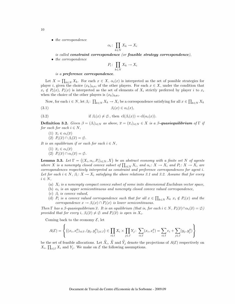
• the correspondenceαi :

∏k∈N

Xk → Xi

is called constraint correspondence (or feasible strategy correspondence),• the correspondence

Pi :∏k∈N

Xk → Xi

is a preference correspondence.

Let X =∏

k∈N Xk. For each x ∈ X, αi(x) is interpreted as the set of possible strategies forplayer i, given the choice (xk)k 6=i of the other players. For each x ∈ X, under the condition thatxi /∈ Pi(x), Pi(x) is interpreted as the set of elements of Xi strictly preferred by player i to xi

when the choice of the other players is (xk)k 6=i.

Now, for each i ∈ N , let βi :∏

k∈N Xk → Xi be a correspondence satisfying for all x ∈∏

k∈N Xk

(3.1) βi(x) ∈ αi(x),

(3.2) if βi(x) 6= 6© , then cl(βi(x)) = cl(αi(x)).

Definition 3.2. Given β = (βi)i∈N as above, x = (xi)i∈N ∈ X is a β-quasiequilibrium of Γ iffor each for each i ∈ N ,

(1) xi ∈ αi(x)(2) Pi(x) ∩ βi(x) = 6©.

It is an equilibrium if or each for each i ∈ N ,(1) xi ∈ αi(x)(2) Pi(x) ∩ αi(x) = 6©.

Lemma 3.3. Let Γ =((Xi, αi, Pi)i∈N , X

)be an abstract economy with a finite set N of agents

where X is a nonempty closed convex subset of∏

i∈N Xi, and αi : X → Xi and Pi : X → Xi arecorrespondences respectively interpreted as constraint and preference correspondences for agent i.Let for each i ∈ N , βi : X → Xi satisfying the above relations 3.1 and 3.2. Assume that for everyi ∈ N ,

(a) Xi is a nonempty compact convex subset of some inite dimensional Euclidean vector space,(b) αi is an upper semicontinuous and nonempty closed convex valued correspondence,(c) βi is convex valued,(d) Pi is a convex valued correspondence such that for all x ∈

∏k∈N Xk xi /∈ Pi(x) and the

correspondence x → βi(x) ∩ Pi(x) is lower semicontinuous.Then Γ has a β-quasiequilibrium x. It is an equilibrium (that is, for each i ∈ N , Pi(x)∩αi(x) = 6©)provided that for every i, βi(x) 6= 6© and Pi(x) is open in Xi.

Coming back to the economy E , let

A(E) =

((xi, x

gi )i∈I , (yj , y

gj )j∈J

)∈

∏i∈I

Xi ×∏j∈J

Yj :∑i∈I

(xi, xgi ) =

∑i∈I

ei +∑j∈J

(yj , ygj )

be the set of feasible allocations. Let Xi, X and Yj denote the projections of A(E) respectively onXi,

∏i∈I Xi and Yj . We make on E the following assumptions.


11

A.1: For each i ∈ I,(a) Xi is convex and closed, and Xi is compact,(b) Pi : Xi ×

∏h6=i πG(Xh) → Xi is lower semicontinuous,

(c) For each (xh, xgh)h∈I ∈ X, Pi

((xi, x

gi ), (x

gh)h6=i

)) is convex,

and (xi, xgi ) ∈ cl Pi

((xi, x

gi ), (x

gh)h6=i

)\ Pi

((xi, x

gi ), (x

gh)h6=i

)),

(d) ei ∈ Xi −∑

j∈J θijYj ;A.2: For each j ∈ J , Yj is convex and closed, and Yj is compact.

The following proposition is proved using Lemma 3.3 and standard techniques explained in [49, 16].

Proposition 3.1. Under Assumptions A.1 and A.2, the private provision economic model E hasa quasiequilibrium

((xi, x

gi )i∈I , (yj , y

gj )j∈J , (p, pg) ∈

∏i∈I Xi ×

∏j∈J Yj × (RL ×RK) \ {0}. Under

the additional continuity assumption that each correspondence Pi has open (in Xi) values at every(xh, xg

h) ∈ X, the quasiequilibrium is nontrivial if∑

i∈I ei ∈ int(∑

i∈I Xi −∑

j∈J Yj

).

Note that the quasiequilibrium price (p, pg) is nonnull but, obviously, not necessarily positive.Replacing in Assumption A.1 (b) by

(b’) Each correspondence Pi : Xi ×∏

h6=i πG(Xh) → Xi has open lower sections in Xi ×∏h6=i πG(Xh) and open (in Xi) values at every (xh, xg

h) ∈ X.the same quasiequilibrium existence result can be proved using as in [14] the definition of Edgeworthequilibria for this kind of constrained preferences, their existence and their decentralization bynonnull quasiequilibrium prices. If the correspondences Pi are convex valued, Assumption (b’) isslightly weaker than the assumption in Shafer–Sonnenschein [50] that the Pi have an open graph,equivalent if correspondences Pi are assumed to have open values for every (xh, xg

h) ∈ X (See aproof of this equivalence in Shafer [48] or in [4]). Our emphasis on the conditions of existence of anon trivial quasiequilibrium is justified by the well-known fact that several irreducibility conditionson the economy guarantee that a non-trivial quasiequilibrium is an equilibrium.

Before closing this section, two remarks are in order.

Remark 3.4. The definition of an abstract economy and the statement of Lemma 3.3 allow forconsidering more externality in consumers’ preferences than the simple existence of public goods.Consumers’ preferences may depend more generally on the current consumption and productionallocation and on current prices as it was demanded by Arrow–Hahn [2]. In particular, Lemma 3.3implies equilibrium existence in exchange economies with only private goods where individualsvalue not only their own consumption but, as in [25], the current consumption allocation.

Remark 3.5. An economy with only private goods and no externality in preferences is a particularcase of the private provision model studied in this section. Proposition 3.1 obviously applies toproduction economies without any public good or externality. This remark will be used in the nextsection.

4. Quasiequilibrium and equilibrium existence in the Lindahl–Foley model

Economy E is now the economy associated with a Lindahl–Foley model as explained in thebeginning of section 2. We assume in particular that consumers have no endowment in publicgoods, thus that for each i ∈ I, ei = (ωi, 0) and that the values of Pi : Xi → Xi does not dependon the consumptions of the other consumers. One could get quasiequilibrium existence in the


12

Lindahl–Foley model using, as for the private provision model, a simultaneous optimization proofbased on a slight modification of the definition and the quasiequilibrium existence result for anabstract economy. This is not the strategy generally adopted sincer Foley [20, 21] and that wefollow now.

We extend3 the commodity space by considering each consumer’s bundle of public goods as aseparate group of commodities. On this (L + |I|K)- dimensional commodity space, we associatewith E the production economy

E ′ =(〈RL × R|I|K , RL × R|I|K〉(X ′

i, P′i , e

′i)i∈I , (Y ′

j )j∈J , (θij) i∈Ij∈J

)defined in the following way:

• For each i ∈ I,– X ′

i = {x′i = (xi, 0, . . . , Gi, . . . , 0) ∈ RL × (RK)|I| : (xi, Gi) ∈ Xi}– e′i = (ωi, 0, . . . , 0, . . . , 0)– For each x′i = (xi, 0, . . . , Gi, . . . , 0) ∈ X ′

i,P ′

i (x′i) = {x′i = (xi, 0, . . . , Gi, . . . , 0) ∈ X ′

i : (xi, Gi) ∈ Pi

((xi, Gi)

)}

• For each j ∈ J , Y ′j = {y′j = (yj , y

gj , . . . , yg

j , . . . , ygj ) ∈ RL × (RK)|I| : (yj , y

gj ) ∈ Yj}.

Let

A(E) =

((xi, G)i∈I , (yj , y

gj )j∈J

)∈

∏i∈I

Xi ×∏j∈J

Yj :∑i∈I

xi =∑i∈I

ωi +∑j∈J

yj ; G =∑j∈J

ygj

denote the set of feasible Lindahl–Foley allocations of E and

A(E ′) =

((x′i)i∈I , (y′j)j∈j

)∈

∏i∈I

X ′i ×

∏j∈J

Y ′j :

∑i∈I

x′i =∑i∈I

e′i +∑j∈J

y′j

denote the set of feasible allocations of E ′. Under the definitions given above,

((x′i)i∈I , (y′j)j∈j

)∈

A(E ′) if and only if((xi, G)i∈I , (yj , y

gj )j∈J

). Let Xi (resp. X ′

i) and Yj (resp. Y ′j ) denote the

projections of A(E) (resp. A(E ′)) on Xi (resp.X ′i) and Yj (resp. Y ′

j ).Economy E ′ is an economy with no public good and no externality. In order to apply to this

economy the quasiequilibrium existence result obtained in the previous section, we set on E thefollowing assumptions.

B.1: For each i ∈ I,(a) Xi = RL

+ × RK+ and Xi is compact,

(b) Pi : Xi → Xi is lower semicontinuous,(c) For each (xi, G) ∈ Xi, Pi(xi, G) is convex,

and (xi, G) ∈ cl Pi(xi, G) \ Pi(xi, G),(d) (ωi, 0) ∈ Xi;

B.2: For each j ∈ J , Yj is convex and closed, contains (0, 0), and Yj is compact.

It is readily seen that if E satisfies these assumptions, then E ′ satisfies the assumptions of Proposi-tion 3.1. Thus, starting from a quasiequilibrium

((x′i)i∈I , (y′j)j∈J , π

)of E ′ with π = (p, (pg

i )i∈I) ∈RL+|I|K \ {0}, and setting pg =

∑i∈I pg

i , one deduces from the definition of X ′i and Y ′

j that

3Independently of Foley, the same strategy was applied in an unpublished paper of F. Fabre-Sender [11], quoted in [42].


13

there exists((xi, G), (yj , y

gj )

)∈

∏i∈I Xi ×

∏j∈J Yj such that

((xi, G), (yj , y

gj ), (p, (pg

i )i∈I))

is aLindahl-Foley quasiequilibrium of E . We have thus proved:

Proposition 4.1. Under the above Assumptions B.1 and B.2, the Lindahl–Foley model E has aquasiequilibrium

((xi, G)i∈I , (yj , y

gj )j∈J , (p, (pg

i )i∈I))∈

∏i∈I Xi ×

∏j∈J Yj ×

((RL ×R|I|K) \ {0}

).

The easy proof of the following corollary can be found in [18] and is sketched here for the sakeof completeness of the paper .

Corollary 4.1. Under the additional continuity assumption that each correspondence Pi has open(in Xi) values at every (xi, G) ∈ Xi, the quasiequilibrium is nontrivial if

NT:∑

i∈I(ωi, 0) ∈ int(RL

+ × RK+ −

∑j∈J Yj

).

Proof. Recalling that the quasiequilibrium price (p, (pgi )i∈I) is nonnull, let (u, v) ∈ RL × RK be

such that (p,∑

i∈I pgi ) · (u, v) < 0 and (

∑i∈I , 0) + (u, v) ∈ (RL

+ × RK+ ) −

∑j∈J Yj . one can write

for some (xi)i∈I ∈ (RL+)I , G ∈ RK

+ , (yj , ygj )j∈J ∈

∏j∈J∑

i∈I

(ωi, 0) + (u, v) =(∑

i∈I

xi, G)−∑j∈J

(yj , ygj

).

One deduces: ∑i∈I

(p · xi + pgi ·G) < p ·

∑i∈I

ωi +∑j∈J

(p,∑

i ∈ Ipgi ) · (yj , y

gj )

≤ p ·∑i∈I

ωi +∑j∈J

(p,∑

i ∈ Ipgi ) · (yj , y

gj ) =

∑i∈I

(p · xi + pgi ·G).

It classically follows that at least one consumer i satisfies at (xi, G) his budget constraint with astrict inequality, and thus is optimal at (xi, G) in his budget set as a consequence of the additionalcontinuity assumption made on consumers’ preferences.

In the following assumption, in order to get informations on respectively the quasiequilibriumprice of private goods and the vector of personalized prices of public goods, the local no-satiationassumption contained in Assumption B.1 (c) is replaced by the stronger assumption of local no-satiation in private goods at any component of a Lindahl–Foley feasible consumption allocation. Atevery Lindahl–Foley feasible consumption allocation, one assumes in addition global no-satiationin public goods for at least one consumer. This is summarized in the following assumption.

B.3: If((xh)h∈I , G) is a Lindahl–Foley feasible consumption allocation,

(a) For each i ∈ I, for every neighborhood U of (xi, G) in Xi, there exists x′i such that(x′i, G) ∈ U and (x′i, G) ∈ Pi((xi, G)),

(b) There exists i ∈ I and Gi such that (xi, Gi) ∈ Xi and (xi, Gi) ∈ Pi((xi, G)).

Under this assumption, the next proposition completes the previous one. One should note that,besides the fact that B.3(a) precises the local no-satiation assumption contained in B.1(c), As-sumptions B.3 (a) and (b) are tailored for getting the conclusions (1) and (2) of the next propo-sition.

Proposition 4.2. Let((xi, G)i∈I , (yj , y

gj )j∈J , (p, (pg

i )i∈I))be the quasiequilibrium obtained in Propo-

sition 4.1. If each correspondence Pi has open (in Xi) values at every (xi, G) ∈ Xi and if Assump-tion B.3 is added to the different assumptions of Proposition 4.1, then


14

(1) The quasiequilibrium price vector for private goods, p, is nonnull, provided that the quasiequi-librium is non-trivial.

(2) If the quasiequilibrium is an equilibrium, then (pgi )i∈I 6= 0.

(3) Under some irreducibility condition, a non-trivial quasiequilibrium is actually an equilib-rium.

Remark 4.2. The non-triviality condition NT is satisfied under the following mild conditionsthat the total initial endowment in private goods is strictly positive and that each public good isproductible:

• ω � 0,• there is some (y, yg) ∈ Y :=

∑j∈J Yj such that yg � 0.

Remark 4.3. The role of an irreducibility assumption is to guarantee that, at the quasiequilibriumprice, all consumers can satisfy with a strict inequality their budget constraint as soon as this ispossible for at least one of them. Such a condition, inspired by Arrow–Hahn [2], was given in [18]:

IR: For any non-trivial partition {I1, I2} of the set I of consumers and for any Lindahl–Foley feasible consumption allocation (xi, G)i∈I , there exists a consumption allocation(xi, G)i∈I and ω such that

• (xi, G) ∈ cl Pi(xi, G) ∀i ∈ I1 with for some i0 ∈ I1, (xi, G) ∈ Pi(xi, G),• (

∑i∈I xi, G) ∈ {(ω, 0)} +

∑j∈J Yj with, for each coordinate ` ∈ L, ω` > ω` ⇒∑

i∈I2ω`

i > 0.The obvious interpretation of this condition is that for any partition {I1, I2} of the set I of con-sumers into two nonempty subgroups and for each feasible allocation, the group I1 may be movedto a preferred position feasible with a new vector of total resources in private goods by increas-ing the total resources of commodities which can be supplied in positive amount by the groupI2. To see how IR is an irreducibilty assumption, let

((xi, G)i∈I , (yj , y

gj )j∈J , (p, (pg

i )i∈I))

be thequasiequilibrium of E , I1 be the set of consumers who can verify their budget constraint with astrict inequality, I2 be the set of consumers for whom this is impossible, a set that we assume tobe nonempty. If (xi, G)i∈I and ω are as in Assumption IR, we can write ω−ω = α

∑i∈I2

(ωi−x′i)with α > 0 and xi ∈ Xi ∀i ∈ I2. Then

p ·∑i∈I1

(xi − ωi) + (∑i∈I1

pgi ) · G >

∑i∈I1

θij

∑j∈J

(p · yj + pg · ygj ),

(1 + α)[p ·

(∑i∈I2

xi + αx′i1 + α

− ωi

)+ (

∑i∈I2

pgi ) ·

G

1 + α

]≥ (1 + α)

∑i∈I2

θij

∑j∈J

(p · yj + pg · ygj ),

that is

p·[∑i∈I2

xi−∑i∈I2

ωi+ω−ω]+(

∑i∈I2

pgi )·G ≥ (1+α)

∑i∈I2

θij

∑j∈J

(p·yj+pg ·ygj ) ≥

∑i∈I2

θij

∑j∈J

(p·yj+pg ·ygj ),

the last inequality following from the positivity of the value of the maximum profit of each producer.Summing in I ∈ I the first and the third of the previous relations, we get

p ·∑i∈I

(xi − ωi) + (∑i∈I

pgi ) · G >

∑j∈J

(p · yj + pg · ygj ),

which contradicts the feasibility for total resources ω of the consumption allocation (xi, G)i∈I .


15

Remark 4.4. In the literature, it is sometimes assumed that each consumer i ∈ I has a strictlypositive initial endowment ωi � 0 and a continuous complete preference preorder �i on his con-sumptin set Xi, weakly monotone relative to public goods and strictly monotone relative to privategoods. Then non-triviality and irreducibilty conditions are of no use and, under the other condi-tions of Proposition 4.1 and Part (b) of Assumption B.3, an equilibrium exists with p � 0 and(pg

i )i∈I > 0 (that is ≥ 0 and not equal to 0).

5. Decentralization with prices of (weakly) Pareto optimal Lindahl–Foleyfeasible consumption allocations

As already noticed, (weak) Pareto optimality of a Lindahl–Foley equilibrium consumption allo-cation simply follows from the definitions. The same is true for Wicksell–Foley public competitiveequilibrium consumption allocations.

Proposition 5.1. Let((xi, G)i∈I , (yj , y


)be a Wicksell–Foley public competi-

tive equilibrium. The consumption allocation (xi, G)i∈I is (weakly) Pareto optimal.

Proof. Assume by contraposition that there is((xi)i∈I , G

)such that (xi, G) ∈ Pi(xi, G) ∀i ∈ I and

(∑

i∈I xi, G) = (∑

i∈I ωi, 0) +∑

j∈J(yj , ygj ). Thus

∑j∈J yj =

∑i∈I(xi − ωi) and

∑j∈J yg

j = G.In view of Condition (1) in Definition 2.3, for every j ∈ J , p · yj + pg · yg ≤ p · yj + pg · yg =πj(p, pg) and by summing on i, p ·

∑j∈J yj + pg · G ≤

∑j∈J πj(p, pg). Let us first set for each

i, ti = p · ωi − p · xi. Summing on i,∑

i∈I ti = −∑

j∈J p · yj ≥ pg · G −∑

j∈J πj(p, pg). If∑i∈I ti = pg · G −

∑j∈J πj(p, pg), the government proposal (G, (ti)i∈I) contradicts Condition

(3) of Definition 2.3. If∑

i∈I ti > pg · G −∑

j∈J πj(p, pg), it suffices to define (t′i)i∈I such thatt′i ≤ ti ∀i ∈ Iand

∑i∈I t′i = pg ·G−

∑j∈J πj(p, pg) to contradict Condition (3) of Definition 2.3,with

the government proposal (G, (t′i)i∈I).

Weak Pareto optimality of Wicksell–Foley public competitive equilibrium allocations is notsurprising. Condition (3) of Definition 2.3 guarantees that, in some sense, the grand coalitioncannot block the equilibrium consumption allocation. In view of Proposition 2.1, (weak) Paretooptimality of Lindahl–Foley feasible consumption allocations, obvious from the simple definitions,is also a consequence of the previous proposition and is nothing else than a statement of the firstwelfare theorem for public goods economies. The purpose of this section is to give converse results.

The next proposition simply extends to convex production sets Theorem of Section 3 in Fo-ley [21].

Proposition 5.2. Assume B.1, B.2, B.3, NT and IR on E. Let((xi, G)i∈I , (yj , y

gj )j∈J

)be a

Lindahl–Foley feasible allocation of E such that (xi, G)i∈I is (weakly) Pareto optimal. Then thereexists a price system (p, (pg

i )i∈I) such that, setting pg =∑

i∈I pgi ,

(1) for every j ∈ J , for every (yj , ygj ) ∈ Yj, (p, pg) · (yj , y

gj ) ≤ (p, pg) · (yj , y

gj ) := πj((p, pg),

(2) for every i ∈ I, (xi, Gi) ∈ Pi(xi, G) implies p · xi + pgi ·Gi > p · xi + pg

i ·G.

Proof. Let

D =

{(z, (Gi)i∈I

)−

(∑i∈I

ωi, 0, . . . , 0, . . . , 0): z =

∑i∈I

xi and (xi, Gi) ∈ Pi(xi, G) ∀i ∈ I

},


16

F =

(y, (yg, . . . , yg, . . . , yg)

): (y, yg) =

∑j∈J

(yj , ygj ) with (yj , y

gj ) ∈ Yj ∀j ∈ J

.

The sets D and F are nonempty, convex and it follows from the (weak) Pareto optimality of theallocation that D ∩ F = 6©. From the first separation theorem, there exists

(p, (pg

i )i∈I

)6= 0 and

α ∈ R such that for all j ∈ J , for all (yj , ygj ) ∈ Yj , for all i ∈ I, for all (xi, Gi) ∈ Pi(xi, G),

p ·∑i∈I

(xi − ωi) +∑i∈I

pgi ·Gi ≥ α ≥ p ·

∑j∈J

yj + (∑i∈I

pgi ) ·

∑j∈J

ygj .

From local no-satiation at each (xi, G), and since((xi, G)i∈I , (yj , y

gj )j∈J

)is a Lindahl–Foley feasible

allocation, we get

p ·∑i∈I

(xi − ωi) + (∑i∈I

pgi ) ·G = α = p ·

∑j∈J

yj + (∑i∈I

pgi ) ·

∑j∈J

ygj .

from which we deduce: for every j ∈ J , for every (yj , ygj ) ∈ Yj , (p,

∑i∈I pg

i )·(yj , ygj ) ≤ (p,

∑i∈I pg

i ))·(yj , y

gj ), and for every i ∈ I, (xi, Gi) ∈ Pi(xi, G) implies p · xi + pg

i ·Gi ≥ p · xi + pgi ·G.

In view of Assumptions NT and IR, one shows exactly as in Section 4 that for every i ∈ I,(xi, Gi) ∈ Pi(xi, G) actually implies p · xi + pg

i ·Gi > p · xi + pgi ·G.

A first corollary of Proposition 5.2 shows that, under the assumptions of the proposition, theset of (weakly) Pareto optimal consumption allocations actually coincides with the set of publiccompetitive equilibrium consumption allocations.

Corollary 5.1. Assume, as in Proposition 5.2, B.1, B.2, B.3, NT and IR on E and that((xi, G)i∈I , (yj , y

gj )j∈J

)is a Lindahl–Foley feasible allocation of E such that (xi, G)i∈I is (weakly)

Pareto optimal. If (p, (pgi )i∈I) is the price vector obtained in Proposition 5.2 and If we set pg =∑

i∈I pgi and for each i ∈ I, ti = p · ωi − p · xi, then

((xi, G)i∈I , (yj , y


)is a

public competitive equilibrium.

Proof. From (1) in Proposition 5.2, the profit maximization is verified. Moreover,∑

i∈I ti =p ·

∑i∈I(ωi − xi) = −p ·

∑j∈J yj = pg · G −

∑j∈J πj(p, pg). If

∑i∈I ti = pg · G −

∑j∈J πj(p, pg)

with for each i ∈ I, (xi, G) ∈ Pi(xi, G), one deduces from (2) in Proposition 5.2: p · xi + pgi ·G >

p · xi + pgi · G ∀i ∈ I, thus p ·

∑i∈I xi +

∑i∈I ti > p

∑i∈I ωi, which proves Condition (3) of

Definition2.3. On the other hand, for each i ∈ I, p · xi + ti = p · ωi and (xi, G) ∈ Pi(xi, G) impliesp · xi > p · xi thus p · xi + ti > p · ωi, which proves Condition (2) of the same definition.

To go further on the decentralization with prices of Lindahl–Foley feasible (weakly) Paretooptimal allocations, notice that in Proposition 5.2,

((xi, G)i∈I , (yj , y

gj )j∈J , (p, (pg

i )i∈I))

correspondsfor the Lindahl–Foley model to what is called valuation equilibrium or equilibrium relative toa price system in an economy with only private goods. In our public goods economy, with respectto the (weak) Pareto optimal consumption allocation (xi, G)i∈I , prices (p, (pg

i )i∈I , pg =

∑i∈I pg

i )have the same normative interpretation as in the usual Second Welfare Theorem. Announced andenforced by a coordinating center, such prices have the property that no consumer will departfrom the Pareto optimal consumption allocation (xi, G)i∈I and that no producer will depart fromthe corresponding production allocation (yj , y

gj )j∈J . The achieved equilibrium corresponds to a


17

vector of individual taxes for public goods equal to (pgi )i∈I and to a vector of individual lump sum

transfers (T i)i∈I , each one equal to

T i = p · xi + pgi ·G−

(p · ωi +

∑j∈J

θijπj(p, pg)),

the sum over i ∈ I of T i being obviously equal to zero.

The interpretation of (p, (pgi )i∈I) in terms of Lindahl–Foley equilibrium prices for a convenient

redistribution of initial endowments and profit shares is more difficult.

A simple corollary of Minkowski–Farkas Lemma (see Corollary 2.3.2. in [19]) gives necessaryand sufficient conditions for finding profit shares (θ′ij) i∈I

j∈J≥ 0 such that

∑j∈J θ′ij = 1 ∀i ∈ I and

for every i ∈ I,

p · xi + pgi ·G = p · ωi +

∑j∈J

θ′ij(p · yj + pg · ygj ) = p · ωi +

∑j∈J

θ′ijπj(p, pg).

Corollary 5.2. Let((xi, G)i∈I , (yj , y

gj )j∈J

)be an equilibrium allocation relative to the price sys-

tem(p, (pg

i )i∈I)). There exists some (endogenous) system of profit shares (θ′ij) i∈I

j∈Jsuch that(

(xi, G)i∈I , (yj , ygj )j∈J , (p, (pg

i )i∈I))

is a Lindahl–Foley equilibrium of the public goods economyE ′ =

((RL

+ × RG+, Pi, (ωi, 0))i∈I , (Yj)j∈J , (θ′ij) i∈I

j∈J

)if and only if for every i ∈ I, for every α ∈ R,

πj(p, pg) ≤ α ∀j ∈ J =⇒ p · (xi − ωi) + pgi ·G ≤ α,

πj(p, pg) ≥ α ∀j ∈ J =⇒ p · (xi − ωi) + pgi ·G ≥ α.

A necessary condition is in particular that for every i ∈ I, p · (xi − ωi) + pgi ·G ≥ 0.

Corollary 5.3. If there is only one producer and if for every i ∈ I, p·(xi−ωi)+pgi ·G ≥ 0, then there

exists an endogenous system of profit shares, (θ′i)i∈I , such that((xi, G)i∈I , (y, G), (p, (pg

i )i∈I))

is aLindahl–Foley equilibrium of the public goods economy E ′ =

((RL

+ × RG+, Pi, (ωi, 0))i∈I , Y, (θ′i)i∈I

).

In this case, defining for every G ∈ RK+ ,

c(G) = min{−p · y : (y, G) ∈ Y } = −max{p · y : (y, G) ∈ Y }

and for every i ∈ I, gi : RK+ → R by

gi(G) = (pgi − θ′ip

g) ·G + θ′ic(G)

then((xi, G)i∈I , (y,G), (gi(G))i∈I

)is what is called in Mas-Colell–Silvestre [40] a linear cost

share equilibrium of the economy E ′.

Proof. The first part of the corollary is actually a particular case of the previous one. Recall that,in view of Assumption B.2, the maximum profit p · y + pg ·G is nonnegative. If p · y + pg ·G > 0,define for each i ∈ I, θ′i = p·(xi−ωi)+pg

i ·Gp·y+pg·G . If p · y + pg · G = 0, define for each i ∈ I, θ′i = 1

|J| .

In both cases,((xi, G)i∈I , (y, G), (p, (pg

i )i∈I))

is a Lindahl–Foley equilibrium of the economy E ′ =((RL

+ × RG+, Pi, (ωi, 0))i∈I , Y, (θ′i)i∈I

).

Let us now turn to the second part. The cost share system verifies∑

i∈I(pgi − θ′ip

g) = 0 and∑i∈I θ′i = 1. On the other hand, in view of the profit maximization at (y, G), c(G) = −p ·G and

for each i ∈ I, gi(G) = pgi · G − θ′i(p · y + pg

i · G), which implies p · xi + gi(G) = p · ωi. Now,


18

(xi, G) ∈ Pi(xi, G) implies p · xi + pgi ·G > p · ωi + θ′i(p · y + pg ·G) ≥ p · ωi + θ′i(p · y + pg ·G) for

all y such that (y, G) ∈ Y , thus p · xi + gi(G) > p · ωi.

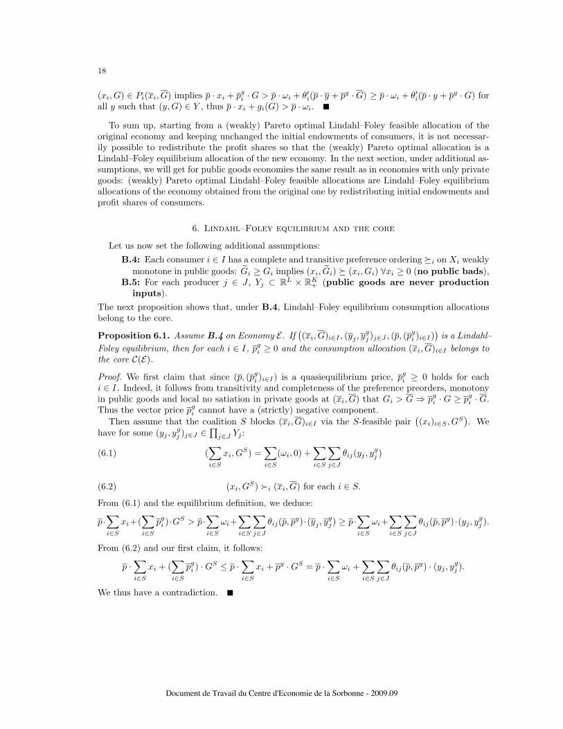
To sum up, starting from a (weakly) Pareto optimal Lindahl–Foley feasible allocation of theoriginal economy and keeping unchanged the initial endowments of consumers, it is not necessar-ily possible to redistribute the profit shares so that the (weakly) Pareto optimal allocation is aLindahl–Foley equilibrium allocation of the new economy. In the next section, under additional as-sumptions, we will get for public goods economies the same result as in economies with only privategoods: (weakly) Pareto optimal Lindahl–Foley feasible allocations are Lindahl–Foley equilibriumallocations of the economy obtained from the original one by redistributing initial endowments andprofit shares of consumers.

6. Lindahl–Foley equilibrium and the core

Let us now set the following additional assumptions:B.4: Each consumer i ∈ I has a complete and transitive preference ordering �i on Xi weakly

monotone in public goods: Gi ≥ Gi implies (xi, Gi) � (xi, Gi) ∀xi ≥ 0 (no public bads),B.5: For each producer j ∈ J , Yj ⊂ RL × RK

+ (public goods are never productioninputs).

The next proposition shows that, under B.4, Lindahl–Foley equilibrium consumption allocationsbelong to the core.

Proposition 6.1. Assume B.4 on Economy E. If((xi, G)i∈I , (yj , y

gj )j∈J , (p, (pg

i )i∈I))is a Lindahl–

Foley equilibrium, then for each i ∈ I, pgi ≥ 0 and the consumption allocation (xi, G)i∈I belongs to

the core C(E).

Proof. We first claim that since (p, (pgi )i∈I) is a quasiequilibrium price, pg

i ≥ 0 holds for eachi ∈ I. Indeed, it follows from transitivity and completeness of the preference preorders, monotonyin public goods and local no satiation in private goods at (xi, G) that Gi > G ⇒ pg

i ·G ≥ pgi ·G.

Thus the vector price pgi cannot have a (strictly) negative component.

Then assume that the coalition S blocks (xi, G)i∈I via the S-feasible pair((xi)i∈S , GS

). We

have for some (yj , ygj )j∈J ∈

∏j∈J Yj :

(6.1) (∑i∈S

xi, GS) =

∑i∈S

(ωi, 0) +∑i∈S

∑j∈J

θij(yj , ygj )

(6.2) (xi, GS) �i (xi, G) for each i ∈ S.

From (6.1) and the equilibrium definition, we deduce:

p·∑i∈S

xi+(∑i∈S

pgi )·G

S > p·∑i∈S

ωi+∑i∈S

∑j∈J

θij(p, pg)·(yj , ygj ) ≥ p·

∑i∈S

ωi+∑i∈S

∑j∈J

θij(p, pg)·(yj , ygj ).

From (6.2) and our first claim, it follows:

p ·∑i∈S

xi + (∑i∈S

pgi ) ·G

S ≤ p ·∑i∈S

xi + pg ·GS = p ·∑i∈S

ωi +∑i∈S

∑j∈J

θij(p, pg) · (yj , ygj ).

We thus have a contradiction.


19

The last proposition shows, under the assumptions B.4 and B.5, the complete symmetry be-tween concepts and optimality properties of Lindahl–Foley equlibrium for a public goods economyand Walras equilibrium for a private goods economy. However, it should be stressed that theseassumptions (made by Foley in [20, 21]) are necessary neither for the existence of Lindahl–Foleyequilibrium nor for the decentralization of (weakly) Pareto optimal Lindahl–Foley feasible alloca-tions with personalized taxes and lump sum transfers.

Proposition 6.2. In addition to the assumptions of Proposition 5.2, assume B.4 and B.5 onthe economy E. Let

((xi, G)i∈I , (yj , y

gj )j∈J

)be a Lindahl–Foley feasible allocation of E such that

(xi, G)i∈I is (weakly) Pareto optimal and let (p, (pgi )i∈I) the price system whose Proposition 5.2 es-

tablishes the existence. The allocation together with the price system is a Lindahl–Foley equilibriumof the economy E ′ =

((RL

+ × RG+, Pi, (ω′

i, 0))i∈I , (Yj)j∈J , (θ′ij) i∈Ij∈J

)for

θ′ij =

{pg

i ·ygj

pg·ygj

if ygj 6= 0

1|I| if yg

j = 0and ω′

i = xi −∑j∈J

θ′ijyj .

Proof. Recall that, in view of NT and IR, p 6= 0 and (pgi )i∈I 6= 0. From B.4 and B.5 and the

definition of the new profit shares, it follows that θ′ij ≥ 0 for every i ∈ I and for every j ∈ J , with forevery j ∈ J ,

∑i∈I θ′ij = 1. Then, for every i ∈ I, p·xi+pg

i ·G = p·ω′i+

∑j∈J θ′ijp·yj +pg

i ·∑

j∈J ygj =

p · ω′i +

∑j∈J θ′ijp · yj +

∑j∈J θ′ijp

g · ygj = p · ω′

i +∑

j∈J θ′ijπj(p, pg) and the proof is complete.

7. Concluding remarks

As Wicksell–Foley public competitive equilibrium is less an equilibrium concept than a char-acterization of (weak) Pareto optimality, we are left at the end of this presentation with twoequilibrium concepts.

The first one according to the analytical point of view adopted in this paper, the second one froman historical point of view since its first elaborations dates back to 1985 [3, 6], is the public goodprivate provision equilibrium. As already noticed, private provision of public goods leads to sub-optimal equilibrium allocations of private and public goods. This drawback, the same which waspointed out by Samuelson, is at the origin of a huge literature on Pareto improving governmentinterventions, beginning with [3, 57], that is at the very time of the definition of public goodsprivate provision equilibrium.

The second one, the Lindahl–Foley equilibrium, dating back to 1967–1970 [20, 21], is the trans-lation of the Lindahl solution refered to by Samuelson. However, most of economists, includingSamuelson himself, deny to this equilibrium the ability of being implemented by any market mech-anism. Lindahl–Foley equilibrium does not satisfy the incentive compatibiity constraint as definedby Hurwicz [32]: equilibrium does not requires that revealing the information necessary for theprice mechanism to function be the best strategy of individual consumers. Here also, a huge lit-erature on mechanism design begins in 1977–1980 with the tentative of resolution of the free-riderproblem by Groves and Ledyard [28, 29]. This literature will tend to substitute the equilibriumof a suitably defined mechanism to the equilibrium of the original economy and to found on thegovernment enforcement of appropriate mechanisms the public economic policy of public goodsmarket economies.


20

References

[1] Arrow, K.J. and G. Debreu, Existence of an equilibrium for a competitive economy. Econo-metrica 22 (1954), 265–290

[2] Arrow, K.J. and F.H.Hahn, General Competitive Analysis. Holden-Day, San Francisco, 1971[3] Bergstrom, T., L. Blume, H.Varian, On the private provision of public goods. Journal of Public

Economics 29 (1986), 25–49[4] Bergstrom, T.C, R.P. Parks, T. Rader, Preferences which have open graphs. Journal of Math-

ematical Economics 3 (1976), 265–268[5] Bonnisseau, J-M., Existence of Lindahl equilibria in economies with nonconvex production

sets. Journal of Economic Theory 54 (1991), 409–416[6] Cornes, R., and T. Sandler, The simple analytics of pure public good provision. Economica

52 (1985), 103–116[7] De Simone, A. and M.G. Graziano, The pure theory of public goods: the case of many

commodities. Journal of Mathematical Economics 40 (2004), 847–868[8] Diamantaras, D. and R.P. Gilles, The pure theory of public goods: Efficiency, decentralization

and the core. International Economic Review 37 (1996), 851–860[9] Diamantaras, D., R.P. Gilles, S. Scotchmer, Decentralization of Pareto optima in economies

with public projects, nonessential private goods and convex costs. Economic Theory 8 (1996),,555–564

[10] Dreze, J. and D. de la Vallee Poussin, A tatonnement process for public goods. Review ofEconomic Studies 38 (1971), 133–150

[11] Fabre-Sender, F., Biens collectifs et biens a qualite variable. CEPREMAP discussion paper(1969)

[12] Florenzano, M., Quasiequilibrium in abstract economies without ordered preferences.CEPREMAP discussion paper 8019 (1980)

[13] Florenzano, M., L’equilibre economique general transitif et intransitif: Problemes d’existence.Monographies du Seminaire d’Econometrie XVI. Editions du CNRS, Paris, 1981

[14] Florenzano, M., Edgeworth equilibria, fuzzy core, and equilibria of a production economywithout ordered preferences. Journal of Mathematical Analysis and Applications 153 (1990),18–36

[15] Florenzano, M., Quasiequilibria in abstract economies: Application to the overlapping model.Journal of Mathematical Analysis and Applications 182 (1994), 616–636

[16] Florenzano, M., General Equilibrium Analysis - Existence and Optimality Properties of Equi-librium. Kluwer, Boston, Dordrecht, London, 2003

[17] Florenzano, M. and V. Iehle, Equilibrium concepts for public goods provision under nonconvexproduction technologies. CES working paper (2009)

[18] Florenzano, M. and E. del Mercato, Edgeworth and Lindahl–Foley equilibria of a generalequilibrium model with private provision of pure public goods. Journal of Public EconomicTheory 29 (2006) 713–740

[19] Florenzano, M. and C. Le Van, Finite dimensional Convexity and Optimization. Springer-Verlag, Berlin Heidelberg New York, 2001

[20] Foley, D.K., Resource allocation and the public sector. Yale Economic Essays 7 (1967) , 45–98[21] Foley, D.K., Lindahl’s solution and the core of an economy with public goods. Econometrica

38 (1970), 66–72


21

[22] Fourgeaud, C., Contribution a l’etude du role des administrations dans la theoriemathematique de l’equilibre et de l’optimum. Econometrica 37 (1969), 307–323

[23] Gale, D. and A. Mas-Colell, An equilibrium existence theorem for a general model withoutordered preferences. Journal of Mathematical Economics 2 (1975), 9–15

[24] Gale, D. and A. Mas-Colell, Corrections to an equilibrium existence theorem for a generalmodel without ordered preferences. Journal of Mathematical Economics 6 (1979), 297–298

[25] Ghosal, S. and H.M. Polemarchakis, Exchange and optimality. Economic Theory 13 (1999),629–642

[26] Gourdel, P., Existence of intransitive equilibria in nonconvex economies. Set-valued Analysis3 (1995), 307–337

[27] Greenberg, J., Efficiency of tax systems financing public goods in general equilibrium analysis.Journal of Economic Theory 11 (1975), 168–195

[28] Groves, T. and Ledyard, J. (1977) Optimal allocation of public goods: A solution to the “freerider problem”. Econometrica 45, pp. 783–809.

[29] Groves, T. and Ledyard, J. (1980) The existence of efficient and incentive compatible equilibriawith public goods. Econometrica 48, pp. 1487–1506.

[30] Hammond, P.J. and A. Villar,Efficiency with non-convexities; Extending the “Scandinavianconsensus” approaches. Scandinavian Journal of Economics 100 (1998), 11–32

[31] Hammond, P.J. and A. Villar, Valuation equilibrium revisited. IVIE WP-AD 98-24[32] Hurwicz, L. (1972) On informationally decentralized systems. In Radner, R. and McGuire, B.

(eds) Decision and Organization, Amsterdam: North Holland Press, pp.[33] Khan, M.A. and R. Vohra, An extension of the second welfare theorem to economies with

nonconvexities and public goods. The Quarterly Journal of Economics 102 (1987), 223–241[34] Lindahl, E., Just taxation–A positive solution. Translated from German: Positive L’osung,

in Die Gerechtigkeit (Lund, 1919) and published in R.A. Musgrave and A.T. Peacock, ed.,Classics in the Theory of Public Finance, NewYork: Macmillan and Co. (1958), 168–176

[35] Lindahl, E., Some controversial questions in the theory of taxation. Translated from German:Einige strittige Fragen der Steuertheorie, in Die WirtschaftstheorievderbGegenwart (Vienna,1928) and published in R.A. Musgrave and A.T. Peacock, eds., Classics in the Theory ofPublic Finance, NewYork: Macmillan and Co. (1958), 214–232

[36] Malinvaud, E., A planning approach to the public good problem. The Sweedish Journal ofEconomics 73 (1971), 96–112

[37] Malinvaud, E., Prices for individual consumption, quantity indicators for collective consump-tion. The Review of Economic Studies 39 (1972), 385–405

[38] Mantel, R.R., General equilibrium and optimal taxes. Journal of Mathematical Economics 2(1975), 187–200

[39] Mas-Colell, A., Efficiency and decentralization in the pure theory of public goods. The Quar-tely Journal of Economics 94 (1980), 625–641

[40] Mas-Colell, A. and J. Silvestre, Cost share equilibria: A Lindahlian approach. Journal ofEconomic Theory 47 (1989), 239–256

[41] Meyer, R.A., Private costs of using public goods. Southern Economic Journal 37 (1971),479–488

[42] Milleron, J-C., Theory of value with public goods: A survey article. Journal of EconomicTheory 5 (1972), 419–477

[43] Mishan, E.J., The relationship between joint products, collective goods, and external effects.The Journal of Political Economy 77 (1969), 329–348


22

[44] Murty, S. Externalities and fundamental nonconvexities: A reconciliation of approaches togeneral equilibrium externality modelling and implications for decentralization. Warwick Eco-nomic Research Papers 756 (2006)

[45] Samuelson, P.A., The pure theory of public expenditure. The Review of Economics and Sta-tistics 36 (1954), 387–389

[46] Samuelson, P.A., Diagrammatic exposition of a theory of public expenditure. The Review ofEconomics and Statistics 37 (1955), 350–356

[47] Sandmo, A., Public goods and the technology of consumption. The Review of EconomicStudies 40 (1973), 517–528

[48] Shafer, W., The non-transitive consumer. Econometrica 42 (1974) 913–919[49] Shafer, W., Equilibrium in economies without ordered preferences or free disposal, Journal of

Mathematical Economics 3 (1976), 135–137[50] Shafer, W. and H. Sonnenschein, Equilibrium in abstract economies without ordered prefer-

ences. Journal of Mathematical Economics 2 (1975), 345–348[51] Shafer, W. and H. Sonnenschein, Equilibrium with externalities, commodity taxation, and

lump-sum transfers. International Economic Review 17 (1976), 601–611[52] Shoven, J.B., General equilibrium with taxes. Journal of Economic Theory 8 (1974), 1–25[53] Sontheimer, K.C., An existence theorem for the second best. Journal of Economic Theory 3

(1971), 1–22[54] Starrett, D., Fundamental nonconvexities in the theory of externalities. Journal of Economic

Theory 4 (1972), 180–199[55] Starrett, D. and P. Zeckhauser, Treating external diseconomies–Market or taxes. Statistical

and Mathematical Aspects of Pollution Problems, J.W. Pratt, ed., Amsterdam, Dekker (1974)[56] Villanacci, A. and E.U. Zenginobuz, Existence and regularity of equilibria in a general equi-

librium model with private provision of a public good. Journal of Mathematical Economics41 (2005), 617–636

[57] Warr, P.,The private provision of public goods is independent of the distribution of income.Economics Letters 13 (1983), 207–211

[58] Weber, S. and H. Wiesmeth, The equivalence of core and cost share equilibria in an economywith a public good. Journal of Economic Theory 54 (1991), 180–197

[59] Weymark, J.A., Existence of equilibria for shared goods. PhD dissertation, Chapter II, De-partment of Economics, University of Pensylvania (1976)

[60] Weymark, J.A., Optimality conditions for public and private goods, Public Finance Quarterly7 (1979), 338–351

[61] Weymark, J.A., Shared consumption: A technological analysis. Annales d’Economie et deStatistiques 75/76 (2004), 175–195 (Substantially revised version of the first chapter of au-thor’s PhD dissertation)

[62] Wicksell, K., A new principle of just taxation. Extracts translated from: Ein nues prinzip dergerechten besteuerung, in Finanztheoristizche Unterschungen, iv-vi, 76–87 and 101–159, 1896,and published in R.A. Musgrave and A.T. Peacock, eds., Classics in the Theory of PublicFinance, NewYork: Macmillan and Co. (1958), 72–118.


Walras-Lindahl-Wicksell: What equilibrium concept for ...

Documents

Transcript of Walras-Lindahl-Wicksell: What equilibrium concept for ...