Wage Posting and Business Cycles:a Quantitative Exploration∗

Giuseppe Moscarini†

Yale Universityand

NBER

Fabien Postel-Vinay‡

University College Londonand

Sciences Po

Revised: August 2015

Abstract

We provide a quantitative exploration of business cycles in a frictional labor mar-ket under contract-posting. The steady-state random search and wage-posting modelof Burdett and Mortensen (1998) has become the canonical structural framework forempirical analysis of worker turnover and equilibrium wage dispersion. In this paper,we provide an efficient algorithm to simulate a dynamic stochastic equilibrium versionof this model, the Stochastic Burdett-Mortensen model, and evaluate its performanceagainst empirical evidence on fluctuations in unemployment, vacancies and wages.

Keywords: Equilibrium Job Search, Dynamic Contracts, Stochastic Dynamics, Busi-ness Cycles.JEL codes: J64, J31, E32.

∗We thank Melvyn Coles and two anonymous referees for very useful comments.†Address: Department of Economics, Yale University, PO Box 208268, New Haven

CT 06520-8268. Tel. +1-203-432-3596. E-mail giuseppe.moscarini@yale.edu. Webhttp://www.econ.yale.edu/faculty1/moscarini.htm . Moscarini thanks the NSF for support tothis research under grant SES 1123021.

‡Address: Department of Economics, University College London, Drayton House, 30 Gordon Street,London WC1H 0AX, UK. Tel: +44 117 928 8431. E-mail fabien.postelvinay@gmail.com. Webhttps://sites.google.com/site/fabienpostelvinay/. Postel-Vinay is also affiliated with the Centrefor Macroeconomics (CfM, London), CEPR (London) and IZA (Bonn).

1 Introduction

Why are similar workers paid differently? In his 2003 book of this title, Dale Mortensen takes

stock of a few decades of investigation of this question, that he had jumpstarted and then

developed. His answer is simple: imperfect competition in labor markets. Information and

other frictions, which make the outcome of job search time-consuming and random, endow

firms with monopsony power that they exploit, in the spirit of Coase (1972), by committing

to wage offers. This force depresses all wages towards the opportunity cost of work. But

workers cannot commit to their current terms of employment and, while employed, search

for better outside offers. In this environment, firms choose a wage policy that balances

labor costs with hiring and retention. As a result, in equilibrium, wages must differ among

identical firms and workers. In the presence of heterogeneity in productivity and in demand

conditions among workers and firms, equilibrium wages still fall short of marginal products,

and contain a non-fundamental component of “frictional” inequality. If workers could freely

reallocate across heterogeneous firms, they would arbitrage away any wage differences.

Burdett and Mortensen (1998, thereafter BM) formalized this powerful insight. Their

working paper, first circulated in the 1980s, spurred the vast theoretical and empirical liter-

ature culminating in Dale Mortensen’s 2003 book. The BM “wage posting” model quickly

emerged as the canonical framework for the analysis of wage inequality, labor turnover, and

unemployment. Each of the three exists in conjunction with the other two. Naturally, the

scope of this line of research eventually transcended wage inequality alone.

In a series of articles (Moscarini and Postel-Vinay 2009, 2011, 2012, 2013, 2014, thereafter

MPV09-MPV14, resp.) we explored, both theoretically and empirically, the business cycle

implications of the wage posting paradigm. Progress in this direction had been stunted by

technical difficulties in finding equilibrium in an economy where the law of one price fails.

The other canonical model of the labor market now known as “DMP” (Diamond, 1982;

Pissarides, 1985; Mortensen and Pissarides, 1994) bypassed this hurdle by assuming that

trading partners bargain over their match surplus, which takes any allocative role away from

wages. The DMP model still encodes the leading theory of equilibrium unemployment, but

runs into difficulties when applied to business cycles. As Shimer (2005) demonstrated, this

model cannot reconcile the large cyclical swings in job finding and unemployment rates with

the tiny ones in Average Labor Productivity (ALP) that we observe in the US economy.

The perfectly competitive labor market model had failed this test, because it required an

implausibly elastic aggregate labor supply. The same issue came back to haunt the search-

cum-bargaining model (Hagedorn and Manovskii, 2008). The attention then turned to other

sources of amplification. We add to this range of new hypotheses. The simple Coasian

1

assumption of commitment to wage offers to exploit market power, here conferred by frictions

and tempered by on-the-job search, is a natural source of wage rigidity, in an environment

that can also explain wage inequality and reallocation and that is very well understood in

steady state since BM.

In our past theoretical work, we outlined the scope and limitations of wage posting mod-

els with random search in the presence of aggregate shocks to labor productivity. Our main

empirical focus was on the cyclical reallocation of employment among heterogenous firms

(MPV12). Our contribution here is to evaluate the quantitative performance of our MPV13

business cycle wage-posting model against empirical evidence regarding not only wage in-

equality and the pace of reallocation, as is standard in this approach, but also business cycle

fluctuations in unemployment and wages. To this end, we propose a tractable, stochastic

equilibrium version of the BM model — we will refer to is as the “Stochastic BM” (SBM)

model — and an operational algorithm to simulate its equilibrium.

Different varieties of wage-posting models with on-the-job search introduced aggregate

shocks and maintained tractability by making one key change to the environment. Menzio

and Shi (2011) assume perfect information about posted wages, in the tradition of directed

or competitive search, and study business cycle movements in labor market quantities, but

not in wages. Closer to our exercise, Robin (2011) maintains random search, but relaxes

the full commitment and equal treatment assumptions, to adopt Postel-Vinay and Robin

(2002)’s sequential auctions, in which firms can respond individually to outside offers received

by their employees. This change greatly simplifies the analysis of business cycles. Robin

addresses empirical evidence on both labor market flows and wages. Relative to these two

contributions, in our SBM model computation of equilibrium wages is less straightforward.

However, we show that it is still feasible, and we propose a reasonably fast algorithm to

achieve this end. We build on the simple structure of the stochastic equilibrium, which

is Rank-Preserving, as first defined in MPV09: more productive and larger firms always

offer higher values to all workers, independently of the history of aggregate shocks. Thus,

workers always move in the same direction between jobs: given the distribution of firm

recruiting effort, equilibrium turnover is trivial to simulate and generates empirically accurate

predictions about job ladder movements over business cycles (MPV14). Our more demanding

task now is to compute the equilibrium recruiting policies and contracts (or state-contingent

wages) that implement this equilibrium allocation.

The broader goal of this project is to provide a unified explanation, based on a stochastic

job ladder, for worker turnover and individual earnings dynamics, residual wage inequality

unexplained by worker characteristics, and business cycle fluctuations in unemployment and

average earnings. This is a very ambitious goal. In this first quantitative step, to give our

2

model a reasonable chance to perform well over business cycles, we introduce a seemingly

minor but important change relative to MPV13. Following Pissarides (2009)’s suggestion,

we model adjustment frictions on the firm side as a cost that depends on the volume of

hires and not, as is customary, of vacancies or job adverts. Search for trading partners is

still mediated by a matching function, but the firm pays for the output of its recruiting

activities, not for the inputs into it. As such, hiring costs are best thought of as training

costs. This feature of the model tames congestion effects that facilitate hiring in recessions,

when unemployment is abundant, and thus mute the negative impact of aggregate shocks on

job creation (see Christiano et al., 2013). This change in the model requires a new argument

to prove that equilibrium retains the RP property, essential for tractability. We find that

this property requires a restriction on the convexity of the hiring/training cost function.1

We gauge the quantitative performance of our SBM model along three main dimen-

sions. First, we assess the model’s ability to amplify TFP shocks, based on its predictions

about the volatility and covariances of unemployment, the job finding rate and the vacancy-

unemployment (V/U) ratio, in the face of TFP shocks of a plausible magnitude. Second,

we examine wage flexibility in the model, as measured by the earnings-unemployment semi-

elasticity (on which we provide new evidence from the Survey of Income and Program Partic-

ipation — SIPP), and the time-series volatility of mean log earnings. Third, we re-examine

the BM model’s predictions about cross-sectional dispersion in wages, profits, and employer

sizes — the focus of many analyses of the steady-state BM model. In so doing, we highlight

new connections between the model’s cross-sectional and business-cycle predictions.

Our summary assessment of the successes and failures of this SBM model is as follows.

A clear success of the SBM model is its ability to generate plausible amplification of TFP

shocks. For example, the predicted volatility ratio of the job finding rate relative to ALP,

which has been the focus of much attention in the literature, can be as high as 15, well in line

with the data. Yet, wages in the SBM model are much more flexible than they appear to be

in the data: the model-based wage-unemployment semi-elasticity is up to ten times larger

than the one we estimate from SIPP data. How, then, does the model generate plausible

amplification? First, even though wages are very flexible, the values that workers care about

and, ultimately, matter for the allocation are much stickier. Second, and most importantly,

the model generates amplification by concentrating hiring amongst firms at the bottom of

the productivity ladder. Those low-productivity firms generate a low surplus, so that even

with flexible wages, small fluctuations in productivity cause large (proportional) variations

1Coles and Mortensen (2012) adopt a hiring cost function and impose on it even more structure, asexplained in Footnote 4, to extend the scope of our early work on transitional dynamics (MPV09). Theyestablish existence and characterization of one RP equilibrium also in the presence of idiosyncratic, firm-levelTFP shocks.

3

in profitability, and consequently on hiring, for those firms (as per the intuition put forward

in a different context by Hagedorn and Manovskii, 2008 and revisited by Ljungqvist and

Sargent, 2015).

This amplification mechanism highlights a trade-off between aggregate volatility of un-

employment and cross-sectional dispersion in employer size. We achieve concentration of

hiring at low-productivity firms by assuming a very highly convex recruitment (or training)

cost function. This strong degree of diminishing returns to hiring tames the incentives of

highly-productive firms to hire much more than low-productivity firms. Dispersion in gross

hiring flows between high- and low- productivity firms is therefore very small and, as a conse-

quence, so is dispersion in equilibrium size between firms. The largest firm in the simulated

economy is only about four times the size of the smallest one, in constrast to millions ob-

served in the data. This tension between size dispersion and amplification is arguably the

key link between the model’s cross-sectional and dynamic predictions.

Next, the SBM model tends to understate cross-sectional wage dispersion. This is not

a new finding: as pointed out by Hornstein, Krusell and Violante (2011), if the residual

wage dispersion observed in US data was truly the result of search frictions, a jobless worker

searching for jobs should wait to sample a high paying job. But average unemployment

duration in the U.S., as measured in the Current Population Survey, is short.2 On-the-job

search helps to resolve this tension, at least qualitatively, because accepting quickly a low

offer does not ‘burn’ all of the option value of looking for a better wage. The SBM model

generates up to two thirds of the residual dispersion in monthly earnings estimated from

the SIPP, under a reasonable calibration of the value of leisure and of measurement error in

earnings. So, while not a complete success, our exercise goes a long way towards addressing

the Hornstein et al. (2011) critique.

Finally, as we highlighted in previous work (MPV13), the model offers a natural expla-

nation for our observation (MPV12) that net job creation is more negatively correlated with

aggregate unemployment at large than at small firms. In the SBM model this still holds,

although, as mentioned, exactly the opposite is true of gross job creation, which is the source

of aggregate volatility in job finding rates. Intuitively, in an aggregate expansion, small em-

ployers hire proportionally more new workers than, but lose even more employees to poaching

by, larger competitors, so their employment grows more slowly on net. The opposite occurs

in recessions, the Great Recession being a perfect example (MPV14).3 The disconnect in

2Using data from the Survey of Income and Program participation (SIPP), Fujita and Moscarini (2013)show that unemployment duration in the US is shortest for the large share of workers who end up beingrecalled by their former employers, and is in fact much longer than commonly thought, even in good times,for those unemployed workers who are hired by new employers, which is presumably what search models arereally about. The CPS does not contain information to make this distinction.

3Kahn and McEntarfer (2014) use matched employer-employee US data to order employers on the job

4

the model between the cyclicality of gross and net job creation among heterogeneous firms

is critical. Bils et al. (2012) show, in a DMP-style model, that a similar tension between

aggregate volatility and cross-sectional inequality on the worker side cannot be resolved.

They observe that the importance of small surplus emphasized by Hagedorn and Manovskii

(2008) applies to the labor supply of the marginal, not the average, worker. Hence, they ask

whether worker ex ante skill heterogeneity can amplify the effect of aggregate shocks on the

average job finding rate, by concentrating job finding volatility among low-skill individuals,

whose surplus from work over leisure is small. They show that this is indeed the case only

if the calibrated model also delivers job finding rates for high wage workers that are far too

sticky relative to the data. Just like large, productive firms exhibit surprisingly cyclical net

job creation rates, so high-wage, productive workers face surprisingly cyclical exit rates from

unemployment. In our exercise, the distinction between gross and net flow, which exists for

an individual firm but not an individual worker, resolves this tension.

The rest of the paper is organized as follows. Section 2 introduces the SBM model and

establishes conditions for equilibrium to be RP, hence computable. Our quantitative analysis

follows in Section 3, which presents empirical moments upon which the calibration and

simulation presented in Section 4 are based. After some concluding remarks, the Appendix

contains the proofs of the formal arguments and presents the structure of the computation

algorithm.

2 A wage-posting model of the business cycle

2.1 The environment

Our Stochastic BM (SBM) model is a variant of MPV13’s business cycle model of a frictional

labor market with random search and wage posting. In this version, we introduce firm-level

hiring costs that depend on the output of the hiring process, namely on the flow of hires,

rather than on the input, vacancies or job ads. So hiring costs are best thought of as a

combination of search and training costs. As emphasized by Pissarides (2009), hiring costs

are independent of competition in the market, hence, unlike vacancy costs, they do not fall

in recessions, when labor demand is lower, and do not mute the effect of aggregate shocks.4

Time t = 0, 1, 2 . . . is discrete. The labor market is populated by a unit-mass of ex ante

homogeneous workers, who can be either employed or unemployed, and by a unit measure of

ladder by the average wage they pay, and find direct evidence for this cyclical poaching pattern.4This assumption is taken up in a growing number of contributions to the topic at hand, including the

closely related paper by Coles and Mortensen (2013). In their paper, recruitment costs are specified asLc(h/L), where L is initial firm size and h is the inflow of new hires, so that h/L is the number of new hiresper incumbent worker in the firm.

5

ex ante heterogeneous firms, which can be either active in production or idle. Workers and

firms are risk neutral, infinitely lived, and maximize payoffs discounted with common factor

β ∈ [0, 1). Firms operate constant-return technologies with labor as the only input and with

productivity scale ωtp, where ωt ∈ Ω is an aggregate component, evolving according to a

stationary first-order Markov processQ (dωt+1 | ωt), and p is a fixed, firm-specific component,

distributed across firms p according to a c.d.f. Γ over some positive interval[p, p

].

The labor market is affected by search frictions in that unemployed workers can only

sample job offers sequentially with some probability λt ∈ (0, 1] at time t and, while searching,

enjoy a value of leisure bt. Employed workers earn a wage and also sample job offers with

probability sλt ∈ (0, 1] each period, so that s is the search intensity of employed relative

to unemployed job seekers. Workers receive at most one job offer per time period. Each

employed worker is separated from his employer and enters unemployment every period with

probability δt ∈ (0, 1]. All firms of equal productivity p start out with the same labor force

L0(p). We denote by Lt(p) the size of a firm of type p at time t on the equilibrium path,

and Nt(p) =∫ p

pLt(x)dΓ(x) the cumulated population distribution of employment across firm

types. So N0(p) is the (given) initial measure of employment at firms of productivity at most

p, Nt (p) is employment and ut = 1−Nt (p) the unemployment (rate) at time t.

We maintain throughout the assumption that the destruction rate is exogenous and a

function of the aggregate productivity state δt = δ (ωt). Similarly for the flow value of non

production bt = b (ωt). The job-contact probability λt instead is determined in equilibrium by

a matching function. Each period, the firm can hire h workers at cost c(h), with c(·) positive,strictly increasing and convex, continuously differentiable. To do so, before workers have a

chance to search, a firm can post a ≥ 0 job adverts (vacancies). Own job adverts determine

the firm’s sampling weight in workers’ job search, while total job adverts determine the rate

at which any one advert returns contacts with workers. Let at(p) denote the adverts posted

on the equilibrium path by a firm of productivity p and size Lt−1(p), and define aggregate

adverts At and aggregate search effort by workers Zt as

At =

∫ p

p

at(p)dΓ(p)

Zt = 1−Nt−1 (p) + (1− δt) sNt−1 (p) .

The latter adds the previously unemployed to the previously employed who are not displaced,

weighted by their search intensity s. In each time period, employed and unemployed search

simultaneously. Then:

ηtAt = λtZt = m (At, Zt) ≤ min ⟨At, Zt⟩

where ηt is the chance for any advert to contact a worker, m(·) is a linearly homogeneous

6

matching function, increasing and concave in each argument.

The timing within a period is as follows. Given a current state ωt of aggregate labor

productivity and distribution of employed workers Nt:

1. firms produce and sell output and pay workers in state ωt; the flow benefit bt accrues

to unemployed workers;

2. the new state ωt+1 of aggregate labor productivity is realized;

3. employed workers can quit to unemployment;

4. filled jobs are destroyed exogenously with chance δt+1;

5. firms post job adverts at+1;

6. the remaining employed workers receive an outside offer with chance sλt+1 and de-

cide whether to accept it or to stay with the current employer; simultaneously, each

previously unemployed worker receives an offer with probability λt+1;

7. firms hire workers and pay hiring costs that depend on how many workers they hire.

Finally, in order to avert unnecessary complications, we assume that the state space Ω

is finite, the distribution of firm types, Γ, has continuous and everywhere strictly positive

density γ = Γ′ over[p, p

], and the initial measure of employment across firm types, N0, is

continuously differentiable in p.

2.2 The firm’s contract-posting and hiring problem

Each firm of any type p chooses and commits to an employment contract, namely a wage

wt(p) contingent on state variables to be specified, to maximize the present discounted value

of profits at time 0, given other firms’ contract offers. The dependence of the wage on the

state is marked for now as a shorthand by the time index of the wage. The firm is further

subjected to an equal treatment constraint, whereby it must pay the same wage to all its

workers. Under commitment, such a wage function implies an equilibrium value Vt(p) for

any worker to work for that firm.

We introduce some notation. Let

Ft (W ) =1

At

∫ p

p

I Vt(p) ≤ W at(p)dΓ(p) (1)

7

(where I· is the indicator function) denote the c.d.f. of values posted by all firms and

offered to searching workers, with F t(·) = 1−Ft(·), i.e. Ft is the distribution of values from

which job searchers draw from,

Gt (W ) =1

Nt−1 (p)·∫ p

p

I Vt(p) ≤ W dNt−1(p) (2)

denote the c.d.f. of values accruing to the currently employed workers. Note that Gt depends

on the distribution of employment Nt−1 at the end of period t−1, i.e. the beginning of period

t, as Nt is determined by Gt itself at the end of the period. Let

Ut = bt + βEt

[(1− λt+1)Ut+1 + λt+1

∫max ⟨v, Ut+1⟩ dFt+1(v)

]be the value of unemployment. The unemployed worker collects a flow value bt and, next

period, when aggregate productivity becomes ωt+1, she draws with chance λt+1 a job offer

from the distribution of offered values Ft+1, that she accepts if its value exceeds that of

staying unemployed. Each firm now has a sampling weight in Ft+1 equal to its (normalized)

job posting, at+1/At+1.

A firm that observes state ωt+1 and decides to post a continuation value Wt+1 < Ut+1

loses all workers, who quit to unemployment, so Lt+1 = 0. In that case, the firm exits, at

least temporarily. Because it cannot be optimal to let all workers go and then hire identical

workers back in the same period, this firm posts no job ads, at+1 = 0, and contributes nothing

to the sampling distribution Ft+1. For the same reason, no worker earns less than Ut, or

Gt(Ut−) = 0. Conversely, a firm of current size Lt posting any value Wt+1 ≥ Ut+1 loses

workers to unemployment, with chance δt+1, and to other firms, if its workers draw offers,

with chance sλt+1, which are more valuable, with chance F t+1 (Wt+1). The firm chooses to

hire ht+1 workers. Formally:

Lt+1 = Lt (1− δt+1)(1− sλt+1F t+1 (Wt+1)

)+ ht+1 (3)

where hires ht+1 = at+1ηt+1Pt+1 (Wt+1) equals the measure of vacancies posted at+1 times

the contact rate of each vacancy ηt+1 times the probability that the offer is accepted:

Pt+1 (Wt+1) =1−Nt (p) + s (1− δt+1)Nt (p)Gt+1 (Wt+1)

Zt+1

(4)

In (4), the denominator is the measure of workers who can make contact, and the numerator

counts only those who accept the offer, namely all the unemployed and only the fraction of

employed who will earn less than Wt+1 by staying where they are.

Three of the payoff-relevant state variables of the firm’s problem are aggregate and ex-

ogenous to the firm. Those are (1) aggregate productivity ωt, (2) the distribution of values

8

offered by all firms Ft, and (3) the cross-section distribution of values earned by currently

employed workers Gt. The latter two are infinite-dimensional and determine the hiring and

retention effects of posting a contract value. In turn, given knowledge of all firms’ strate-

gies, Nt−1 is sufficient to calculate Gt. Again, these three state variables, ωt, Ft, Nt−1 are

aggregate and exogenous to the firm: for notational simplicity, we subsume the dependence

on all three of firms’ and workers’ values into a time index.

The firm’s problem can be formulated recursively (Spear and Srivastava, 1987) by in-

troducing an additional, fictitious state variable, namely the continuation utility V that the

firm promised at time t− 1 to deliver to the worker from this period t onwards. So the firm

solves

Πt

(V , Lt

)= sup

wt≥0ht+1≥0

Wt+1≥Ut+1

⟨(ωtp− wt)Lt + βEt [−c (ht+1) + Πt+1 (Wt+1, Lt+1)]

⟩(5)

subject to the law of motion (3) of firm size and a Promise-Keeping (PK) constraint to

deliver the promised V :

V = wt + βEt

[δt+1Ut+1 + (1− δt+1)

(1− sλt+1F t+1 (Wt+1)

)Wt+1

+ (1− δt+1) sλt+1

∫ +∞

Wt+1

vdFt+1(v)

]. (6)

Expectations are taken with respect to the future realization ωt+1 of aggregate produc-

tivity and offer distribution Ft+1, conditional on ωt, Ft, Nt−1.

To characterize the best response contract, we first describe an equivalent unconstrained

recursive formulation of the contract-posting problem. We define the joint value of the firm

and its existing workers:

St = Πt + V Lt.

Solving for the wage wt from (6), replacing it into the firm’s Bellman equation (5), and using

(3) to replace the expression for Lt+1 into St+1 = Πt+1 +Wt+1Lt+1 in each future state, the

joint value function St solves the unconstrained, recursive maximization of the joint value of

the firm-worker collective:

St (p, Lt) = ωtpLt + βEt

[δt+1LtUt+1

+ supht+1≥0

Wt+1≥Ut+1

⟨(1− δt+1) sλt+1Lt

∫ +∞

Wt+1

vdFt+1(v)− c (ht+1) + St+1 (p, Lt+1)−Wt+1ht+1

⟩](7)

9

The joint value St to the firm of type p and to its existing Lt employees depends on these

two and on aggregate state variables subsumed in the time index. This joint value equals

flow output, ωtpLt, plus the discounted expected continuation value. The latter includes

(in order) the value of unemployment for those employees who are displaced exogenously,

the value of a new job for those who are not displaced and find a better offer than the one

extended by the current firm, minus the cost of hiring new workers, and, on the second line,

the joint continuation value of the firm and of its current (time t) employees. In turn, the

latter equals the joint continuation value St+1 of the firm and its future workforce — made

up of stayers among the current (date-t) workforce plus next-period (date-t + 1) hires —

minus the value to be paid to new hires, either from unemployment or from other firms.5

The optimal policy solving the unconstrained DP problem (7) also solves (5) subject to

(6). We therefore focus on the analysis of the simpler problem (7). We restrict attention to

Markov equilibria, where the value offered by each firm depends exclusively on payoff-relevant

variables, and not directly on the history of play.

Definition 1 A Markov (contract-posting) equilibrium is a pair of measurable

functions (V,H) of firm-specific productivity p, firm size L, aggregate productivity ω, and ag-

gregate distribution of employment N such that, for every firm type p, if all other firms of type

x play (V,H) so that (1), (2) and (3) hold with Wt = Vt(x) where Vt(x) = V (x, Lt−1(x), ωt, Nt−1)

and ht = Ht(x) where Ht(x) = H (x, Lt−1(x), ωt, Nt−1), the value-posting function Vt(p), the

wage function that implements it (i.e. solves (6) with V = Vt(p)) and the hiring function

Ht(p) are the optimal policies of the contracting problem (5).

An equilibrium is a fixed point, a solution (V,H) to this DP problem that coincides with

the strategy followed by the other firms. The reason why Markov strategies do not depend

on the offer distribution Ft, given the employment distribution Nt−1, is simple. Given the

equilibrium value-offer strategy V and the employment distribution Nt−1, any firm of type

p can compute for every competitor x the probability Gt (Vt(x)) from (2) and thus the

acceptance probability Pt (Vt(x)) from (4). Given the equilibrium hiring strategy H, firm p

can then derive the required vacancy posting at(x) = Ht(x)/ηtPt (Vt(x)) of any other firms

x. Finally, Ft derives from (1). So knowledge of equilibrium strategies (a requirement of

Nash equilibrium) and of the employment distribution Nt−1 suffice to characterize all other

infinite-dimensional state variables.5If we did not subtract this cost of employing new hires, this Bellman equation would generate the joint

value of the firm and all of its workers, current and future. If this were the object maximized by the firm,it would optimally offer its workers the maximum value, i.e. pay a wage equal to productivity (the proof,omitted, is available upon request). As is standard, the efficient solution to a moral hazard problem is to“sell the firm to the workers”. In our economy, however, firms do not pursue efficiency, but maximize profits.Therefore, the optimal value-offer policy is an interior solution.

10

2.3 Rank-Preserving Equilibrium (RPE)

2.3.1 Definition of RPE

The main difficulty in characterizing equilibrium in BM’s environment in the presence of

aggregate uncertainty, which hampered progress of this approach in the analysis of business

cycles, is now clear. The distributions of values offered Ft and earned Gt are relevant to the

firm maximization problem, because they determine the retention rate Ft(W ) of the firm’s

employees who are offered a contract of value W , and the poaching rate from other firms.

This is a defining property of a random search, wage posting model. Even in the simpler

Markov equilibrium the employment distribution Nt−1 at the end of the previous period is

a state variable of the firm problem. Although the firm does not directly control them, it

must still keep track of stochastically and endogenously evolving distributions, an infinitely

complex problem.

An even simpler class of Markov equilibria circumvents this hurdle.

Definition 2 A Rank-Preserving Equilibrium (RPE) is a Markov equilibrium such

that, on the equilibrium path, a more productive firm always offers its workers a higher

continuation value: Vt(p) = V (p, Lt−1(p), ωt, Nt−1) is increasing in p, including the effect of

p on firm size Lt−1(p).

As a direct consequence of the above definition, in a RPE, workers rank their preferences

to work for different firms according to firm productivity at all dates. The RP property

holds in the unique steady-state equilibrium characterized by BM. Definition 2 proposes to

extend it to a dynamic stochastic equilibrium with endogenous hiring.

2.3.2 A characterization result

The key contribution of MPV13 is the proof that, in BM’s original environment with ex-

ogenous (but stochastic) contact rates, any Markov equilibrium must be Rank-Preserving

under some restrictions on firm entry (see below), and under the weak sufficient condition

that more productive firms start weakly larger at time 0. Thus, for any history of real-

izations of aggregate shocks, more productive and larger firms always offer their workers a

higher value, which is the only available tool to control both hiring and retention. Therefore,

the size ranking of firms is preserved over time: if Lt(p) ≥ Lt (p′) for p > p′ at date t, then

Lt+1(p) > Lt+1 (p′). Thus, by induction, Lt+n(p) > Lt+n (p

′) for all positive integers n: if a

more productive firm is ever larger, it will remain larger for ever no matter what happens to

aggregate productivity, because it will always offer a higher value to retain its workers and

hire more workers. Furthermore, the equilibrium evolution of the employment distribution

11

is the same in any RPE, so it is uniquely pinned down, and can be calculated independently

of equilibrium contracts.

In this paper, we add a hiring choice h to the firm’s problem. The RP property alone

therefore no longer suffices to ensure that more productive firms also hire more and, conse-

quently, always remain larger. Offering a higher value only guarantees a better retention of

existing employees, a reduction in the outflow, but firm size also depends on the gross hiring

inflow h. Therefore, the conditions for the unique equilibrium of any kind to be RP, as in

MPV13, are slightly stronger, and the argument for the preservation of size ranking is not

as straightforward. Yet we show in the following proposition that this property continues to

hold in that case.

Proposition 1 (RPE with Hiring Costs) Assume that the hiring cost function c(·) is

C 2, with c′(h) > 0 for all h > 0. Then any Markov contract-posting Equilibrium such that

the sampling c.d.f. Ft(·) is everywhere differentiable at all dates t is Rank-Preserving if:

1. more productive firms are weakly larger at the initial date, i.e. L0(p) is non-decreasing

2. hc′′(h)/c′(h) ≥ 1, i.e. the elasticity of the marginal hiring cost c′(·) is everywhere largerthan 1.

In any such RPE, size ranking is preserved at all dates: Lt(·) is non-decreasing at all t.

Proof. See Appendix A. Proposition 1 extends the characterization result of MPV13 to the case of endogenous

hiring, where firms face recruitment costs that are a function of their gross hiring inflow. It

states sufficient conditions for any Markov equilibrium of our model to be RP.6 This simple

equilibrium allows for cyclical entry and exit “at the bottom”. Because the offered value is

increasing in p, and must exceed the value of unemployment Ut for the firm to be active,

there exists a cutoff productivity such that only firms (if any) below that cutoff will be idle

in each period. This cutoff varies with the aggregate productivity state, thus generating

flctuations in entry and exit.

Condition 2 in Proposition 1, which requires that the training cost function be sufficiently

convex, is a new requirement compared to the result in MPV13. We will return to this

condition in Section 4 below. Apart from that, Condition 1 was already present — and

discussed — in MPV13. This is a genuine restriction for a RPE. However, it is merely a

sufficient condition: it aligns two separate motives to pay workers more, firm productivity

6The restriction to differentiable sampling c.d.f.’s simplifies the proof, but we suspect it is inessential - itis not imposed in MPV13.

12

and size, so there is some slack. Moreover, as explained in MPV13, it is a property that

arises “naturally” in the BM model, insofar as the steady-state distribution of firm sizes in

the BM model satisfies it. As mentioned, the model can generate cyclical firm entry. Entry

of firms “in the middle” of the productivity distribution, however, is ruled out as inconsistent

with RPE: profitable business opportunities may arise and cause entry of highly productive

firms, which by definition start out with a size of zero and are therefore likely to “break

ranks” (see MPV13 for an extended discussion).

With exogenous hiring policies, as we showed in MPV13, the equilibrium allocation, or

evolution of the firm size distribution, is uniquely determined, independently of the specific

value strategies (wage contracts) that implement it, and is simple to compute. In MPV13

we provide sufficient conditions for uniqueness also of RPE contracts, hence of Markov

equilibrium, in the exogenous contact rate model. Our focus here is on computation of one

equilibrium. We leave the question of uniqueness of equilibrium allocations and contracts in

this hiring cost model for future research.

2.3.3 Some useful properties of RPE

Three properties thus hold true in any RPE. First, the share of firms that offer less than

Vt(p) is simply the proportion of firms that are less productive than p weighted by their

relative vacancy postings

Ft (Vt(p)) =1

At

∫ p

p

at(x)dΓ(x). (8)

Second, the share of employed workers who earn a value that is lower than that offered by

p equals the share of employment at firms less productive than p:

Gt (Vt(p)) =Nt−1(p)

Nt−1 (p). (9)

Third, the probability that an offer is accepted equals

Pt (Vt(p)) =1−Nt−1 (p) + s (1− δt)Nt−1(p)

1−Nt−1 (p) + s (1− δt)Nt−1 (p):= Yt(p).

Therefore the sampling weight is at(p) = Ht(p)/ (ηtYt(p)), and we can write it as a function

of the chosen hiring flow. As we will see shortly, these restrictions drastically simplify the

computation of equilibrium in the stochastic model.

In MPV13 we further establish that on the RPE path the joint value St (p, L) of a firm

of type p and of its L employees is differentiable in L. Our focus in this paper being on

computation, we restrict attention to differentiable equilibria without formally extending

MPV13’s differentiability proof to the case of endogenous hiring. We define the costate

13

variable

µt(p) =∂St

∂L(p, L(p))

which is the shadow marginal value of an additional worker to the firm-employees collective.

Using the RP implications (8) and (9) in the Bellman equation (7), differentiating the latter

on both sides with respect to Lt, and invoking the Envelope theorem:

µt(p) = ωtp+ βEt

[δt+1Ut+1 + (1− δt+1)

(1− sλt+1

At+1

∫ p

p

at+1(x)dΓ(x)

)µt+1(p)

+ (1− δt+1)sλt+1

At+1

∫ p

p

at+1(x)Vt+1(x)dΓ(x)

](10)

where in the last integral we changed variable from value V ∼ Ft to productivity p ∼ Γ.

The equilibrium policies Vt (p) and Ht (p) solve the NFOCs for the maximization of (7):

[W ] : Ht(p) = [µt(p)− Vt(p)] (1− δt) sλtLt−1ft (Vt(p))

[h] : c′ (Ht(p)) = µt(p)− Vt(p).(11)

Next, noticing that (8) implies

ft (Vt(p)) =dFt (Vt(p))

dVt(p)=

dFt (Vt(p))

dp

1

V ′t (p)

=at(p)

At

γ(p)

V ′t (p)

,

we can rewrite the FOC for W as

Ht(p) = [µt(p)− Vt(p)] (1− δt) sλtLt−1(p)at(p)

At

γ(p)

V ′t (p)

(12)

Together with the law of motion of employment, equations (10), (11) and (12) are the

backbone of an algorithm to describe the evolution of the equilibrium of this economy subject

to aggregate shocks. The algorithm computes an approximation to the equilibrium contract

in which each firm, while still viewing aggregate productivity ωt+1 as random and taking the

conditional expectation in (10) w.r.t. this random variable, evaluates the future marginal

value of a new employee µt+1(p) in the r.h.s. of (10) as if the period-t realized employment

distribution Nt were always the one occurring on the equilibrium path N⋆t , regardless of

ωt. That firms make this approximation is common knowledge (so each firm knows that

other firms do so, and computes accordingly the distribution of offers made by competitors).

Moreover, firms understand that the period-t employment distribution Nt indeed varies with

ωt and use the correct period-t employment distribution that occurs in each aggregate state

ωt in the computation of the conditional expectation in (10), except for the evaluation of

µt+1(p). The quality of the numerical approximation rests on the twofold observation that the

employment distribution, in the data as well as in our calibration of exact RPE dynamics,

14

moves slowly, and that the marginal value of a worker µt(p) is much more responsive to

variations in ωt than to variations in the other aggregate state variable, Nt−1. We provide

the details of this algorithm in Appendix B.

3 Data

3.1 Labor market and productivity

Most of the aggregate time series that we exploit to either calibrate or test the model

are available at monthly frequency. Nonetheless, we sample and filter them at quarterly

frequency, because Total Factor Productivity (TFP) and Average Labor Productivity (ALP)

series are available only quarterly. To maintain consistency with these data, we calibrate and

simulate the model at monthly frequency, then aggregate its output to quarterly frequency.

The unemployment rate is the civilian unemployment rate of the US population aged 16

and up from the BLS, starting in 1948:Q1 through 2015:Q1. We calculate transition rates

between labor market states Employment (E) and Unemployment (U), using stocks of E and

U and flows EU and UE from monthly CPS matched files (BLS “Research series on labor

force status flows from the CPS”) beginning in 1990:Q1, through 2014:Q4. We do not use

unemployment-duration based measures, nor do we correct for time aggregation (Shimer,

2012), and we treat any short spell of unemployment that completes within a month, and is

missed by monthly CPS interviews, as a continuous employment spell. We make the latter

choice for two reasons: the model is calibrated monthly, so workers there have no chance

to make more than one transition per month, and in the data a majority of very short

unemployment spells end in recall by the same employer (Fujita and Moscarini, 2013).

The V/U ratio is the ratio between the JOLTS vacancy rate (currently available for

2010:Q4-2015:Q2) for the US private nonfarm sector and the civilian unemployment rate.7

For TFP we use quarterly estimates of the Solow residual by Fernald (2012), and for ALP

we take Output per job in the Nonfarm business sector from the BLS (series PRS85006163),

both in 1948:Q1-2015:Q1.

We log and HP-filter all quarterly time series, labor market stocks and flows with param-

eter 100,000, productivity series with parameter 1,600. We then compute second moments

for all observations up to 2012:Q4 included, excluding 2013-2015 to avoid end-of-period HP

filtering bias, although this makes little difference. Although the vacancy and worker flow

7This ratio is routinely referred to as labor market tightness in the context of the DMP model. However,the relevant concept of market tightness in our model, which features on-the-job search, is not the V/U ratio:rather, it is the ratio of vacancies to total worker search effort, U + s(1− δ)(1− U). Because the V/U ratiohas been the focus of much attention in the literature, we report statistics pertaining to that variable, eventhough it does not have a straightforward interpretation within the context of our model.

15

series are available for a much shorter time span than the rest, we use all the available data to

filter each series and, except for the last two years, to compute volatilities and correlations.

We prefer to take this approach rather than to shorten our sample to the longest period

when they are all available, but we should keep in mind that some second moments refer to

shorter subperiods than others.

We report in Table 3, in rows indicated by (D) for Data, standard deviations (last number

on each row) and correlation coefficients of the filtered components of each series. In addition

to the numbers report in Table 3, the data tell us that (detrended log) TFP has a volatility

of 0.127 (about the same as ALP — see Table 3), and correlation −0.4 with detrended log

unemployment. Finally, the first-order serial correlation of log-TFP is 0.78. Based on this,

we remark that TFP and ALP have similar volatilities, an order of magnitude smaller than

that of the (log) unemployment rate, but TFP, unlike ALP, has a strong negative correlation

with the unemployment rate. This reflects in part the fact that our filtered ALP measure

turned slightly countercyclical since the 1980s.

3.2 Wages

We use the 1996, 2000, 2004 and 2008 panels of the Survey of Income and Program Partici-

pation (SIPP). This is a collection of panels of workers, on average about 40,000 workers per

panel. Each worker is surveyed every four months about events that occurred over the past

four months (‘wave’). Workers are assigned to rotation groups: in each calendar month,

roughly one quarter of the panel completes a wave and is re-interviewed. The SIPP has

significant longitudinal and time dimensions, provides information about a large number of

individual outcomes, and is nationally representative.

As the model has no intensive margin of labor supply, for our measure of wages we take

monthly earnings (TPMSUM), which are also less contaminated by measurement error than

hourly pay rates, especially those constructed as the ratio of earnings to “usual hours worked

per month”. We deflate earnings with monthly CPI and take logs. A “seam bias” arises from

a tendency of SIPP respondents to bunch reported changes in earnings and labor market

status around interview times. Rotation groups are staggered, however, so seams are evenly

distributed over time. The only exceptions are the first four and last three months of each

panel, when no rotation group has a seam, but excluding those months has little impact on

the results.

We aim to extract information about the cyclical component of earnings for comparable

workers, as our model has homogeneous workers. To this purpose, we run, with both monthly

and quarterly data, a fixed effect regression of individual real log earnings, constructed as

described above, on the detrended unemployment rate, a common linear trend, a cubic in age,

16

log earnings monthly quarterly

(1) (2) (3) (4)

unemployment rate −.60(.11)

−.50(.11)

−.58(.11)

−.49(.11)

25-99 employees .065(.004)

.062(.004)

100+ employees .078(.005)

.075(.005)

observations (i, t) 2, 910, 524 986, 149

workers (i) 82, 036 81, 457

Varit(errors) .18 .18 .16 .16

R2 .22 .23 .23 .24

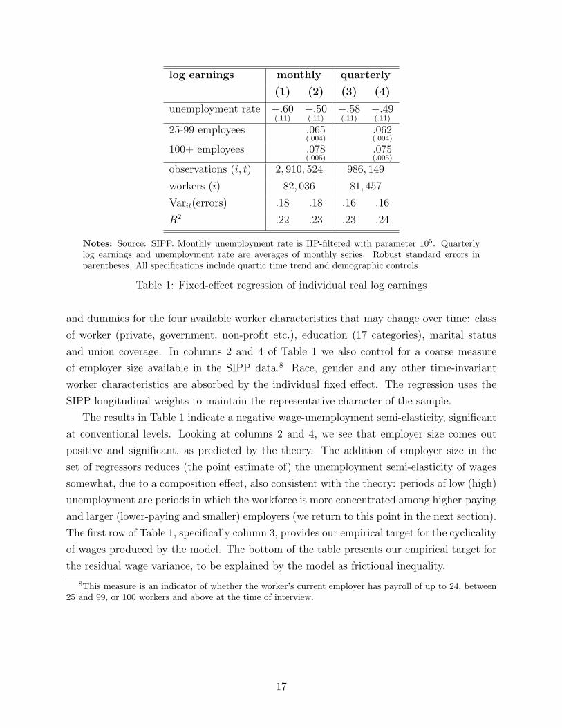
Notes: Source: SIPP. Monthly unemployment rate is HP-filtered with parameter 105. Quarterlylog earnings and unemployment rate are averages of monthly series. Robust standard errors inparentheses. All specifications include quartic time trend and demographic controls.

Table 1: Fixed-effect regression of individual real log earnings

and dummies for the four available worker characteristics that may change over time: class

of worker (private, government, non-profit etc.), education (17 categories), marital status

and union coverage. In columns 2 and 4 of Table 1 we also control for a coarse measure

of employer size available in the SIPP data.8 Race, gender and any other time-invariant

worker characteristics are absorbed by the individual fixed effect. The regression uses the

SIPP longitudinal weights to maintain the representative character of the sample.

The results in Table 1 indicate a negative wage-unemployment semi-elasticity, significant

at conventional levels. Looking at columns 2 and 4, we see that employer size comes out

positive and significant, as predicted by the theory. The addition of employer size in the

set of regressors reduces (the point estimate of) the unemployment semi-elasticity of wages

somewhat, due to a composition effect, also consistent with the theory: periods of low (high)

unemployment are periods in which the workforce is more concentrated among higher-paying

and larger (lower-paying and smaller) employers (we return to this point in the next section).

The first row of Table 1, specifically column 3, provides our empirical target for the cyclicality

of wages produced by the model. The bottom of the table presents our empirical target for

the residual wage variance, to be explained by the model as frictional inequality.

8This measure is an indicator of whether the worker’s current employer has payroll of up to 24, between25 and 99, or 100 workers and above at the time of interview.

17

4 Calibration and simulation

In order to gauge the business cycle properties of the model, we begin with a detailed analysis

of a baseline calibration, which is designed to maximize the model’s ability to replicate the

observed levels of cylical volatility in unemployment and in the job finding rate. Attaining

this goal requires a few “unconventional” choices of parameter values. We subsequently

assess the model’s performance under more conventional parameterizations.

4.1 Baseline calibration

We specify the aggregate shock process as a discrete 20-state first-order Markov chain that

approximates a monthly AR(1) process for lnω. The AR coefficient (0.94) and the variance

of innovations (0.006) are set such that the model replicates the observed variance and first-

order autocorrelation of HP-detrended output per worker.9

The job destruction rate is allowed to fluctuate deterministically with ω as follows:

δ(ω) = 0.0114 + 1.894× (lnωmax − lnω)2.5

where the intercept, slope and exponents in this definition are chosen to approximate the

mean, standard deviation, (positive) skewness and kurtosis of the observed EU rate.

All other parameter values and functional form assumptions are summarized in Table 2.

The distribution of firm types is a truncated Pareto distribution, with the top firm being 10

times as productive as the worst one that could ever operate in the economy. The discount

factor is the monthly equivalent of a 5% discount rate per annum. The employed search

intensity s is set to match an average monthly EE transition rate of around 1.2%, in line

with SIPP data.10 The matching function is simply a linear function of the aggregate number

of job adverts. This differs from the more commonly used Cobb-Douglas specification with a

vacancy elasticity of 0.5, and as such calls for some comments. First, there is some evidence

that the estimated vacancy elasticity of the matching function is substantially higher than 0.5

when employed job seekers are counted as inputs into the matching process (Petrongolo and

Pissarides, 2001).11 Second, the standard procedure in the empirical literature that produced

9Output per worker does not exactly coincide with ω in the model because of the gradual selection ofworkers up the job ladder, but it turns out to be very close.

10There are many different ways to define EE transitions in the SIPP (or any other) data. Here we allowfor up to seven days of non-employment between jobs, and up to a month for “voluntary” EE transitions,i.e. when respondents stated that they quit their past job to take another one. Adding “involuntary” EEtransitions (in the form of forced job-to-job reallocations, as for instance in Jolivet et al., 2006) would be astraightforward extension.

11Even when on-the-job search is ignored, recent estimates by Borowczyk-Martins et al. (2013) thataccount for the endogeneity of vacancies in the presence of reallocation shocks suggest that the matchingfunction elasticity may be higher than commonly assumed, in the region of 0.8.

18

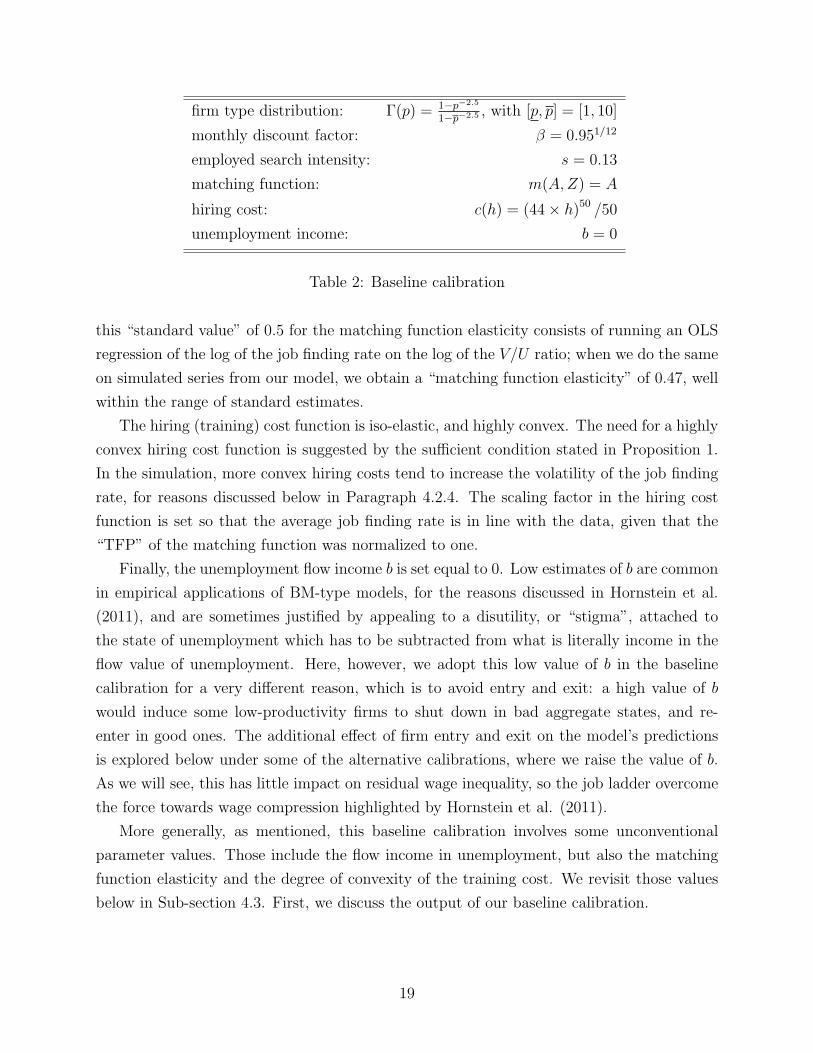
firm type distribution: Γ(p) = 1−p−2.5

1−p−2.5 , with [p, p] = [1, 10]

monthly discount factor: β = 0.951/12

employed search intensity: s = 0.13

matching function: m(A,Z) = A

hiring cost: c(h) = (44× h)50 /50

unemployment income: b = 0

Table 2: Baseline calibration

this “standard value” of 0.5 for the matching function elasticity consists of running an OLS

regression of the log of the job finding rate on the log of the V/U ratio; when we do the same

on simulated series from our model, we obtain a “matching function elasticity” of 0.47, well

within the range of standard estimates.

The hiring (training) cost function is iso-elastic, and highly convex. The need for a highly

convex hiring cost function is suggested by the sufficient condition stated in Proposition 1.

In the simulation, more convex hiring costs tend to increase the volatility of the job finding

rate, for reasons discussed below in Paragraph 4.2.4. The scaling factor in the hiring cost

function is set so that the average job finding rate is in line with the data, given that the

“TFP” of the matching function was normalized to one.

Finally, the unemployment flow income b is set equal to 0. Low estimates of b are common

in empirical applications of BM-type models, for the reasons discussed in Hornstein et al.

(2011), and are sometimes justified by appealing to a disutility, or “stigma”, attached to

the state of unemployment which has to be subtracted from what is literally income in the

flow value of unemployment. Here, however, we adopt this low value of b in the baseline

calibration for a very different reason, which is to avoid entry and exit: a high value of b

would induce some low-productivity firms to shut down in bad aggregate states, and re-

enter in good ones. The additional effect of firm entry and exit on the model’s predictions

is explored below under some of the alternative calibrations, where we raise the value of b.

As we will see, this has little impact on residual wage inequality, so the job ladder overcome

the force towards wage compression highlighted by Hornstein et al. (2011).

More generally, as mentioned, this baseline calibration involves some unconventional

parameter values. Those include the flow income in unemployment, but also the matching

function elasticity and the degree of convexity of the training cost. We revisit those values

below in Sub-section 4.3. First, we discuss the output of our baseline calibration.

19

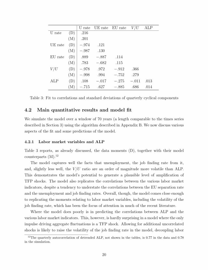
U rate UE rate EU rate V/U ALPU rate (D) .216

(M) .201

UE rate (D) −.974 .121

(M) −.987 .130

EU rate (D) .889 −.887 .114

(M) .783 −.682 .115

V/U (D) −.978 .972 −.912 .366

(M) −.998 .994 −.752 .279

ALP (D) .108 −.017 −.275 −.011 .013

(M) −.715 .627 −.885 .686 .014

Table 3: Fit to correlations and standard deviations of quarterly cyclical components

4.2 Main quantitative results and model fit

We simulate the model over a window of 70 years (a length comparable to the times series

described in Section 3) using the algorithm described in Appendix B. We now discuss various

aspects of the fit and some predictions of the model.

4.2.1 Labor market variables and ALP

Table 3 reports, as already discussed, the data moments (D), together with their model

counterparts (M).12

The model captures well the facts that unemployment, the job finding rate from it,

and, slightly less well, the V/U ratio are an order of magnitude more volatile than ALP.

This demonstrates the model’s potential to generate a plausible level of amplification of

TFP shocks. The model also replicates the correlations between the various labor market

indicators, despite a tendency to understate the correlations between the EU separation rate

and the unemployment and job finding rates. Overall, though, the model comes close enough

to replicating the moments relating to labor market variables, including the volatility of the

job finding rate, which has been the focus of attention in much of the recent literature.

Where the model does poorly is in predicting the correlations between ALP and the

various labor market indicators. This, however, is hardly surprising in a model where the only

impulse driving aggregate fluctuations is a TFP shock. Allowing for additional uncorrelated

shocks is likely to raise the volatility of the job finding rate in the model, decoupling labor

12The quarterly autocorrelation of detrended ALP, not shown in the tables, is 0.77 in the data and 0.78in the simulation.

20

market indicators from ALP.13

4.2.2 Wages

We construct a model-predicted semi-elasticity of wages (real monthly earnings) to the un-

employment rate by running a weighted OLS regression of firm-level log wages on a constant

and on the detrended unemployment rate, with weights equal to Lt(p)γ(p). This is the clos-

est we can get, using the model, to the worker-level regressions reported in Table 1. The

predicted semi-elasticity thus computed (at quarterly frequency) is −7.90. Comparison of

this number with the value of -0.6 reported in the last column of Table 1 suggests that wages

are much more procyclical in the model than in the data. The predicted semi-elasticity drops

a little to −6.97 when firm size is included among the covariates in the aforementioned re-

gression. While this drop parallels the drop seen between columns 3 and 4 of Table 1, the

predicted semi-elasticity is still far too large.

As another point of comparison, the quarterly unit labor cost series produced by the BLS

over the period 1947-2013 has a cyclical volatility of 0.016 (after taking logs and HP-filtering

with parameter 1,600). The model counterpart of this number is 0.065, further corroborating

the conclusion that predicted mean wages are too cyclical. Although wages in the model

are allocative, they merely serve to implement worker values that drive the allocation of

employment in the model. Worker values are more informative than wages in this model.

Their standard deviation is 0.035 at quarterly frequency, and their unemployment semi-

elasticity is −2.07. Worker values are thus substantially less volatile than wages in the

model: forward-looking values anticipate future mean-reversion in wages, and smooth wage

fluctuations. In fact, the mechanism is best understood in reverse. Job creation depends on

the firms’ present value of profits, the difference between output streams and values paid to

workers. In order for profits to be sufficiently procyclical to generate the desired volatility

in job finding rates, worker values must be relatively smooth, but not completely acyclical.

Wages have to respond strongly to aggregate shocks in order to generate some movement in

those forward-looking values.

The literature pointed at excess wage volatility to understand the failure of Nash bar-

gaining models to generate much amplification of TFP shocks. But Ljunqvist and Sargent

(2015), elaborating on Hagedorn and Manovskii (2008), argue that the responsiveness of

wages to TFP shocks is in fact not necessary for amplification, and emphasize the size of the

surplus of matches. This theme emerges also here.

As discussed in the Introduction, one of the key contributions of our SBM model is that

13Shocks to the matching technology or to the job destruction rate come to mind as natural candidates.A recent papers by Hall (2014) makes a case for a countercyclical discount factor.

21

it generates endogenous cross-sectional wage dispersion and as such makes predictions on

second- and higher-order moments of the wage distribution. Focusing on cross-sectional wage

dispersion, the pooled cross-section wage variance predicted by the model is 0.08. This falls

far short of the residual variance of 0.18 found in the SIPP data and reported in Table 1.

Some of that 0.18 variance is arguably attributable to measurement error. Lemieux (2006)

reports a share of around a third, based on CPS data on wage rates. Applied here, this

share would imply a genuine residual log earnings variance of 0.12 in the SIPP. While our

model’s 0.08 still falls short even of this target, it makes very significant progress. The failure

to replicate the observed amount of residual wage dispersion — at least under “standard”

parameterizations — is a well-known and recurring problem of wage posting models (see

Hornstein et al., 2011, and the discussion in our Introduction), from which our SBM dynamic

contract posting model is not immune. On the job search, however, goes a long way towards

resolving this conundrum. Davis and von Wachter (2012), using the DMP model with a

job ladder proposed by Burgess and Turon (2010), conclude that on the job search falls far

short of this task. Our contract-posting model does much better. One reason is that workers

moving from job to job compare values, not wages, and values are much more compressed

than wages (as mentioned, standard deviation 0.035, or variance 0.0012). In turn, this occurs

because even values offered by low-productivity firms contain the option value of climbing

to more productive firms.

Finally, we can address the cyclical behavior of wage inequality. A number of recent

papers have documented the fact that idiosyncratic wage risk, broadly defined as the cross-

sectional standard deviation of wage growth, is countercyclical (Storesletten, Tamer and

Yaron, 2004). The predicted correlation between the cross-section standard deviation of log

wage growth and the (detrended) unemployment rate is 0.23.14 The model thus replicates,

at least qualitatively, the counter-cyclicality of wage risk found in the data.

4.2.3 Profits and worker values

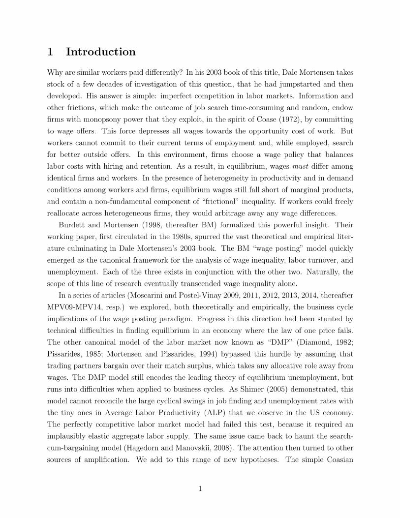
Figure 1a plots the profile of (log) values posted by each firm, lnVt(p), as a function of the

quantiles of p in the distribution Γ, over time. Figure 1b does the same for the (log) prof-

itability of the marginal job in any given firm type, ln [µt(p)− Vt(p)]. As per the properties

of RPE, Vt(p) is increasing in p at all dates. Figure 1b suggests that this is also the case for

marginal profitability, although this result is not guaranteed in theory.

A closer look at Figure 1b further reveals that job profitability is much more cyclically

14The model-predicted standard deviation of wage growth is constructed by taking the standard deviationof firm-level wages weighted by initial employment at each firm. Thus, by design, it measures the wage riskfaced by job stayers.

22

10.8

0.6

Γ(p)

0.40.2

00

50

100

quarters

150

200

250

10.02

10.04

10.06

10.08

10.1

10.12

10.14

10.16

10.18

10.2

10.22

300

(a) Worker values

10.8

0.6

Γ(p)

0.40.2

00

50

100

quarters

150

200

250

14

12

10

8

6

4

2300

(b) Profits

Fig. 1: Marginal profits and worker values over time

10.8

0.6

Γ(p)

0.40.2

00

50

100

quarters

150

200

250

0.023

0.0235

0.024

0.0245

0.025

0.0255

0.026

0.0265

0.027

300

(a) Hires

10.8

0.6

Γ(p)

0.40.2

00

50

100

quarters

150

200

250

2.5

2

1.5

1

0.5300

(b) Job adverts

Fig. 2: Firm-level job adverts and hiring flows over time

sensitive at low-productivity firms than at the top end of the productivity distribution.

This is because jobs at low-productivity firms generate smaller surplus than jobs at high-

productivity firms, and their value is therefore more elastic to TFP shocks. Interestingly,

Figure 1a suggests that this difference in cyclicality across firm types is not passed on to

worker values. This is because these values account for the possibility of moving down the

ladder, where profits are volatile, and are also driven by very volatile job finding rates.

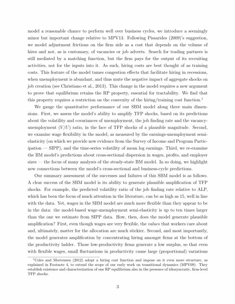
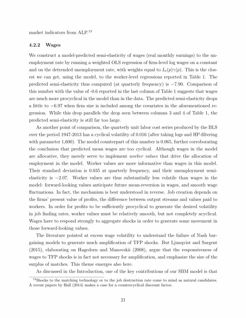
4.2.4 Job adverts, hiring flows, and firm size

Proposition 1 states that in RPE, a firm that is more productive and initially larger than

another stays larger period after period. But it says nothing about whether more productive

firms actually hire more or merely retain a larger fraction of their initial workforce by posting

more attractive job values. Figure 2 provides an answer. Figure 2a plots the profile of

firm-level hiring flows, Ht(p) (still as functions of the quantiles of p in the distribution

23

Γ) over time, while Figure 2b plots the profile of firm-level job adverts, at(p). It appears

that Ht(p) is mostly, although not always strictly increasing in p, while at(p) is decreasing:

more productive firms tend to hire a larger inflow of workers at most dates, but manage

to do so by spending less effort on hiring, simply through the fact that they offer more

attractive job values, thus enjoying a higher job-ad yield. Figure 2 further shows that job

adverts, and therefore hires, are much more cyclically sensitive at low-productivity than at

high-productivity firms, echoing the similar remark made above about profitability of the

marginal job. The firm’s hiring decision is indeed governed by the FOC (11), which imposes

equality between the cost of the marginal hire (c′(h), an increasing function of h), and its

profitability, µ(p)− V (p).

Another remarkable feature of Figure 2a is the lack of dispersion in the level of gross

hiring inflows across firm types. On average over the simulated sample, the most productive

firm in the market only hires 12.5% more workers per quarter than the least productive

one. This is in spite of a 10-fold difference in productivity between the highest- and lowest-

productivity employer in this economy. As a further consequence, the model vastly under-

predicts dispersion in firm sizes: the predicted size ratio between the smallest and largest

employer in the economy is 4.24 on average, nowhere near the levels observed in the data.

The reason for this lack of dispersion in employer size and hiring inflow is the very high

degree of convexity of the hiring cost function c(·). As mentioned Sub-section 4.1, this high

degree of convexity is needed for the model to amplify TFP shocks to the extent observed in

the data. In that sense, the model faces a tradeoff between time-series volatility and cross-

sectional dispersion. As seen on Figures 1 and 2, profitability and (consequently) hiring

and job-ad posting are much more volatile at low-productivity than at high-productivity

firms, as the former generate a much smaller surplus than the latter. In order to inflate

the volatility of aggregate job adverts, the model needs to concentrate hiring among low-

productivity firms. The highly convex training cost does exactly that: it curtails hiring at

high-p firms, which are much more profitable than low-p firms but face prohibitive marginal

training costs beyond a modest level of hiring.

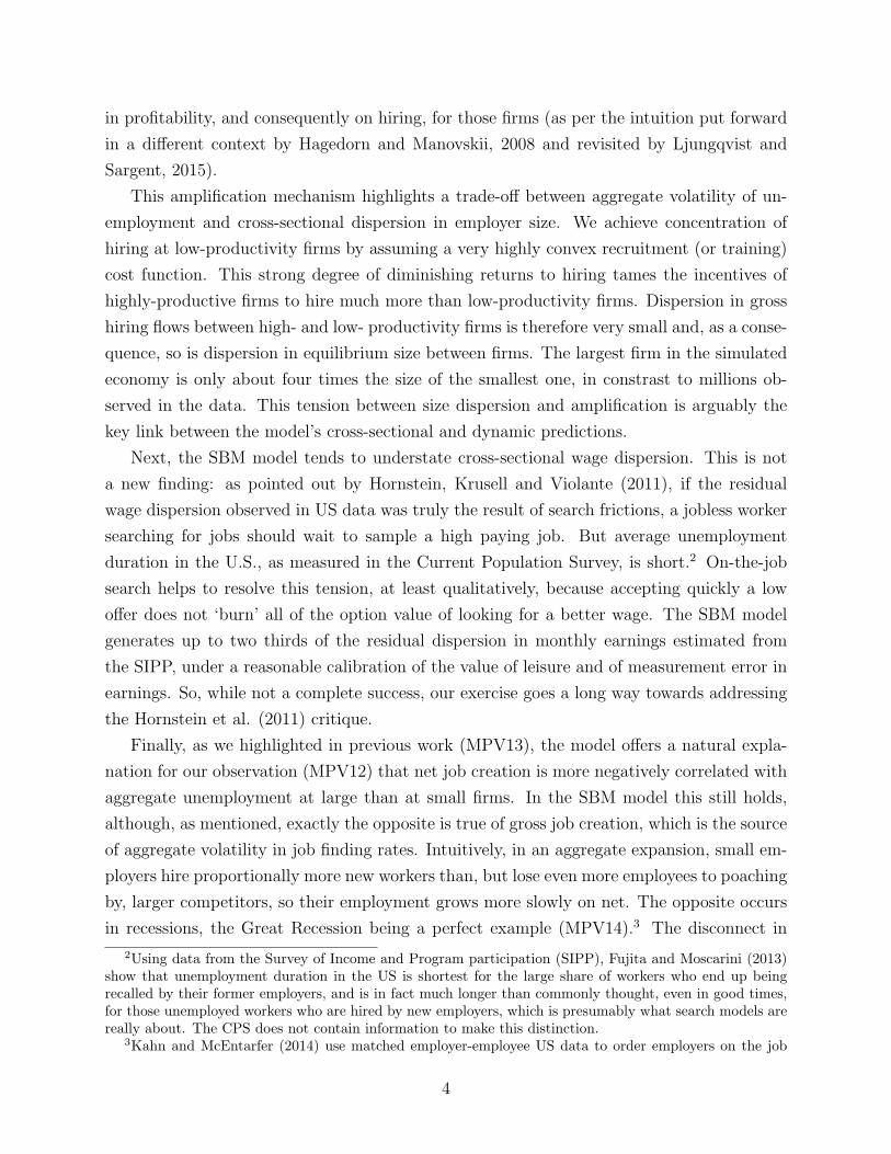
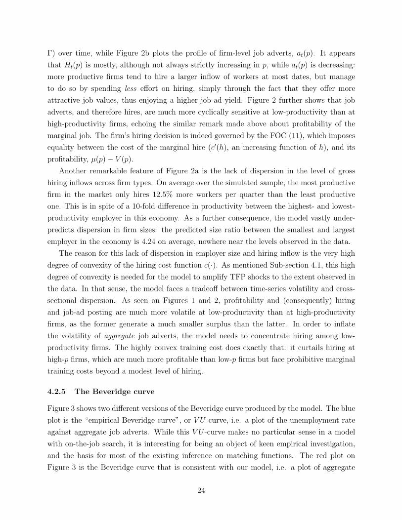
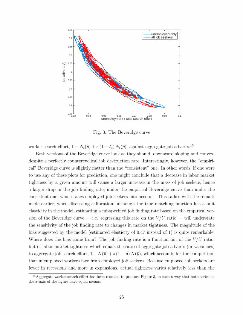
4.2.5 The Beveridge curve

Figure 3 shows two different versions of the Beveridge curve produced by the model. The blue

plot is the “empirical Beveridge curve”, or V U -curve, i.e. a plot of the unemployment rate

against aggregate job adverts. While this V U -curve makes no particular sense in a model

with on-the-job search, it is interesting for being an object of keen empirical investigation,

and the basis for most of the existing inference on matching functions. The red plot on

Figure 3 is the Beveridge curve that is consistent with our model, i.e. a plot of aggregate

24

unemployment / total search effort0.03 0.04 0.05 0.06 0.07 0.08 0.09 0.1

job

adve

rts

At

0.75

0.8

0.85

0.9

0.95

1

1.05

1.1

1.15

1.2

1.25

unemployed onlyall job seekers

Fig. 3: The Beveridge curve

worker search effort, 1−Nt(p) + s (1− δt)Nt(p), against aggregate job adverts.15

Both versions of the Beveridge curve look as they should, downward sloping and convex,

despite a perfectly countercyclical job destruction rate. Interestingly, however, the “empiri-

cal” Beveridge curve is slightly flatter than the “consistent” one. In other words, if one were

to use any of these plots for prediction, one might conclude that a decrease in labor market

tightness by a given amount will cause a larger increase in the mass of job seekers, hence

a larger drop in the job finding rate, under the empirical Beveridge curve than under the

consistent one, which takes employed job seekers into account. This tallies with the remark

made earlier, when discussing calibration: although the true matching function has a unit

elasticity in the model, estimating a misspecified job finding rate based on the empirical ver-

sion of the Beveridge curve — i.e. regressing this rate on the V/U ratio — will understate

the sensitivity of the job finding rate to changes in market tightness. The magnitude of the

bias suggested by the model (estimated elasticity of 0.47 instead of 1) is quite remarkable.

Where does the bias come from? The job finding rate is a function not of the V/U ratio,

but of labor market tightness which equals the ratio of aggregate job adverts (or vacancies)

to aggregate job search effort, 1−N(p)+ s (1− δ)N(p), which accounts for the competition

that unemployed workers face from employed job seekers. Because employed job seekers are

fewer in recessions and more in expansions, actual tightness varies relatively less than the

15Aggregate worker search effort has been rescaled to produce Figure 3, in such a way that both series onthe x-axis of the figure have equal means.

25

V/U ratio over the cycle, which explains the lower estimated elasticity of the job finding rate

to the V/U ratio than to tightness.

4.2.6 The cyclicality of net job creation

As pointed out earlier, gross job creation is muchmore cyclical among small, low-productivity

employers than at the top end of the productivity distribution. Yet in MPV12 we highlight

that, in US data, exactly the opposite is true of net job creation: as a group, small employers

fare relatively better in bad times of high unemployment, and worse in good times of low

unemployment. As we propose in other work (MPV09, MPV14), this empirical pattern is

qualitatively consistent with job ladder models, of which this paper offers a new example:

in a tight labor market, high-paying, large employers overcome the scarcity of unemployed

job applicants by poaching employees from smaller, less productive and lower-paying com-

petitors, whose employment share then shrinks in relative terms. When the expansion ends,

large employers, that were less constrained, have more employment to shed than small ones.

In addition, the resulting high unemployment relaxes hiring constraints on all employers,

particularly the small ones that are less capable of poaching from other firms. As a result,

small employers downsize less in the recession and grow (relatively) faster in the recovery.

This mechanism is at work here. To put a number on its magnitude, we construct

series of total net job creation among two groups of firms, one at the top and one at the

bottom of the productivity ladder, both classes being re-designed at each date so that they

each have an employment share of 25%. We then subtract net job creation in the group

of low-p firms from net job creation in the group of high-p firms, and HP-detrend this

difference to obtain a measure of relative net job creation similar to the series we analyzed

in MPV13. The correlation of this simulated series of relative net job creation with the

simulated unemployment rate is −0.87: as expected, the relative net job creation of large vs.

small employers is procyclical. How plausible the magnitude of that predicted correlation

is appears hard to assess, for lack of immediately comparable data. In MPV13 we report

numbers for U.S. data that vary between −0.25 and −0.6, depending on the data set, period,

sector, etc. Again, the correlation produced by the model is on the high side of that range,

something that is to be expected as the outcome of a one-shock model.

As discussed in the Introduction, the disconnect between gross hires and net employment

growth that exists at multi-worker firms is critical to understand our empirical observations,

and model predictions: large, high-productivity firms have much more procyclical net em-

ployment growth than bottom firms, but much less procyclical gross hires, which are what

matters for aggregate job finding rates. We conclude that the basic insight of Hagedorn and

Manovskii (2008) applies to the bottom of the job ladder, where the surplus is small, and is

26

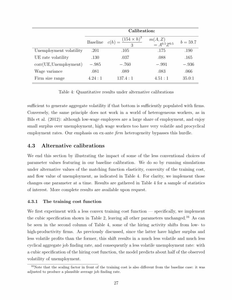
Calibration:

Baseline c(h) =(154× h)3

3

m(A,Z)= A0.5Z0.5 b = 59.7

Unemployment volatility .201 .105 .175 .190

UE rate volatility .130 .037 .088 .165

corr(UE,Unemployment) −.985 −.760 −.991 −.936

Wage variance .081 .089 .083 .066

Firm size range 4.24 : 1 137.4 : 1 4.51 : 1 35.0:1

Table 4: Quantitative results under alternative calibrations

sufficient to generate aggregate volatility if that bottom is sufficiently populated with firms.

Conversely, the same principle does not work in a world of heterogeneous workers, as in

Bils et al. (2012): although low-wage employees are a large share of employment, and enjoy

small surplus over unemployment, high wage workers too have very volatile and procyclical

employment rates. Our emphasis on ex-ante firm heterogeneity bypasses this hurdle.

4.3 Alternative calibrations

We end this section by illustrating the impact of some of the less conventional choices of

parameter values featuring in our baseline calibration. We do so by running simulations

under alternative values of the matching function elasticity, convexity of the training cost,

and flow value of unemployment, as indicated in Table 4. For clarity, we implement those

changes one parameter at a time. Results are gathered in Table 4 for a sample of statistics

of interest. More complete results are available upon request.

4.3.1 The training cost function

We first experiment with a less convex training cost function — specifically, we implement

the cubic specification shown in Table 2, leaving all other parameters unchanged.16 As can

be seen in the second column of Table 4, some of the hiring activity shifts from low- to

high-productivity firms. As previously discussed, since the latter have higher surplus and

less volatile profits than the former, this shift results in a much less volatile and much less

cyclical aggregate job finding rate, and consequently a less volatile unemployment rate: with

a cubic specification of the hiring cost function, the model predicts about half of the observed

volatility of unemployment.

16Note that the scaling factor in front of the training cost is also different from the baseline case: it wasadjusted to produce a plausible average job finding rate.

27

Yet, reflecting the trade-off between volatility and dispersion highlighted above, reducing

the convexity of the hiring cost increases the dispersion in employer sizes substantially. The

size ratio between the largest and smallest firm in the economy is now 137.4 on average.

While this still falls short of observed magnitudes, it is considerably higher than the 4.24

ratio found under the baseline calibration. The cross-sectional dispersion of wages also

increases as a result of the same composition effect. The predicted wage variance under this

specific cubic specification is 0.089, higher than in the baseline case.

4.3.2 The matching function

We next experiment with a matching function elasticity of 0.5, which is arguably at the

opposite extreme of the range of elasticities found in the literature compared to our baseline,

linear-in-job postings specification. This change has remarkably little impact on the simu-

lated statistics reported in Table 4: unemployment and the job finding rate are little less

volatile, wages and employer sizes are marginally more dispersed than in the baseline case,

but those differences are small and within the range of simulation noise.

Unsurprisingly, the difference between this and our baseline calibration is in the esti-

mated matching function. While the true matching function elasticity is 0.5, a regression

of the job finding rate on the V/U ratio (which, once again, replicates standard practice in

matching function estimation) produces a coefficient of 0.29, well below the range of pub-

lished empirical results. This result motivates our choice of a linear matching function in

the baseline calibration.

4.3.3 The value of unemployment, firm entry and firm exit

In our final calibration variant, we set the flow value of unemployment to b = 59.7, equal

across all aggregate states. This puts b at about 50% of the mean wage in the economy. The

main novelty under this alternative calibration is that entry and exit of firms now occurs at

the low end of the productivity distribution: in times of relatively low aggregate productivity

ω, the marginally profitable firm type is in the interior of[p, p

], and fluctuates with ω.17 As

expected, the measure of active firms is procyclical in this model, with a correlation of −0.57

with unemployment at quarterly frequency. Looking at firm entry — i.e. the one-period

change in the measure of active firms — reveals that entry leads unemployment by about

17Allowing for entry and exit requires some additions to the algorithm described in Appendix B. Inparticular, the decision to enter or exit is based on total firm value S (p, Lt(p)) (more precisely, a firm willexit in states where the continuation value in (7) falls short of the value of shutting down, i.e. Ut+1Lt(p)).The algorithm as described in Appendix B only computes the value µt(p) = ∂S (p, Lt(p)) /∂L of the marginalworker in any given firm. Allowing for entry and exit thus requires the additional computation of S (p, Lt(p))along the equilibrium path. Details are available upon request.

28

four quarters. The correlation of unemployment and the four-quarter lag of the change in the

measure of active firms is −0.19, whereas the contemporaneous correlation between those

two variables is a positive 0.16.

Next turning to the results in Table 4, one sees that raising the value of unemployment

has very little effect on the predicted amount of amplification. If anything, unemployment

volatility is a little lower in this high-b variant than in the baseline, b = 0 case, but the

difference is well within the range of simulation noise. This similarity, however, is the net

result of two opposing forces. First, the main force generating amplification, namely the

fact that job creation is concentrated at marginally profitable firms with low surplus, is

still at work and even strenghened now: when unemployment income is high, the surplus

of marginal firms, which are prone to entry and exit, is very close to zero — and in any

case smaller than the surplus of low-productivity firms in the b = 0 case, where even type-p

firms make a positive surplus in all aggregate states. This makes the low-productivity end

of the population of active firms more volatile in the high-b than in the b = 0 case and

tends to further amplify TFP shocks. Yet, with a high b causing entry and exit, those low-

surplus firms get weeded out in recessions, and only enter, with an initial workforce of zero,

in good aggregate conditions. As a result, employment ends up being more concentrated at

higher-surplus firms (firms with higher p) which survive recessions and maintain a positive

workforce, even in bad times. It turns out that those two opposing effects have similar

magnitudes in this calibration.

As could have been predicted based on the insight of Hornstein et al. (2011), a higher

value of unemployment further reduces the amount of cross-sectional wage dispersion pre-

dicted by the model, which, however, remains sizable. Finally, the range of firm sizes is

wider, again due to entry and exit of firms at the low end of the productivity scale. Those

marginal firms see their workforce reset to zero each time they exit, and as a result stay very

small on average over time.

5 Concluding remarks

The wage-posting model of the labor market with random search is one of the most influential

and enduring contributions of Dale Mortensen and his students. The main goal of this paper

is to show that this canonical model of the labor market naturally belongs in the toolbox

of business cycle theorists. We study its quantitative performance and confront it with

empirical evidence from the US. This is our first step in this direction and, as such, is truly

exploratory in nature.

Our exercise reveals dimensions on which the model performs well, and also a fundamental

29

tension between its predictions for aggregate volatility and for cross-sectional inequality in

wages and firm size. We emphasize that this tension emerges precisely because the model is

unusually equipped to address both sides of this trade-off, inequality and cyclical volatility.

In this regard, the model generates business cycles of the correct magnitude by exploiting

firm heterogeneity, in particular, the concentration of gross hires among unproductive, small,

cyclically sensitive firms. This is more than offset by a strong cyclical response of job to job

quits, so that net job creation is more volatile among large firms, a prediction that in previous

work we argued to be shared by many job ladder models, and that we validated empirically

in MPV13. We also find promise in the model’s ability to generate cyclical comovement of

the empirically correct sign between unemployment and wage levels, wage inequality, worker

turnover. Much work lies ahead to identify suitable specifications and parameterizations of

hiring costs, state-contingent contracts, search effort that may further improve the model’s

quantitative performance along these dimensions.

We believe that additional insights from this stochastic job ladder model lie ahead. An

especially promising direction is understanding individual earnings dynamics, the focus of

the incomplete market literature, their relationship to labor market transitions, up and down

the job ladder, and their cyclicality.

References

[1] Bils, Mark, Y. Chang and S. Kim, (2012) “Comparative advantage and unemployment”,

Journal of Monetary Economics, 59(2), 150-165.

[2] Bontemps, C., J.-M. Robin and G. J. Van den Berg (2000) “Equilibrium Search with

Continuous Productivity Dispersion: Theory and Nonparametric Estimation”, Interna-

tional Economic Review, 41(2), 305-358.

[3] Borowczyk-Martins, D., G. Jolivet and F. Postel-Vinay (2013) “Accounting for Endo-

geneity in Matching Function Estimation”, Review of Economic Dynamics, 16, 440-51.

[4] Burdett, K. and D. T. Mortensen (1998) “Wage Differentials, Employer Size and Un-

employment”, International Economic Review, 39, 257-73. [BM]

[5] Burgess, S. and H. Turon (2010) “Worker Flows, Job Flows and Unemployment in a

Matching Model.” European Economic Review, 54(3), 393408.

[6] Christiano, L., M. Eichenbaum and M. Trabandt (2013) “Unemployment and Business

Cycles”, Northwestern University mimeo.

30

[7] Coase, R. (1972) “Durability and Monopoly”, Journal of Law and Economics, 15(1),

143-49.

[8] Coles, M. and D. T. Mortensen (2013) “Equilibrium Wage and Employment Dynamics

in a Model of Wage Posting without Commitment” NBER WP 17284.

[9] Davis, S. and T. von Wachter (2012) “Recessions and the Costs of Job Loss”. Brookings

Papers on Economic Activity, April 2012.

[10] Diamond, P. A. (1971) “A Model of Price Adjustment”, Journal of Economic Theory,

3, 156-168.

[11] Diamond, P. A. (1982) “Aggregate Demand Management in Search Equilibrium”, Jour-

nal of Political Economy, 90(5), 881-894.

[12] Fernald, J. (2012) “A Quarterly, Utilization-Adjusted Series on Total Factor Produc-

tivity”, Working Paper Series 2012-19, Federal Reserve Bank of San Francisco.

[13] Fujita, S. and G. Moscarini (2013) “Recall and Unemployment”, NBER WP No. 19640.

[14] Hagedorn, M. and I. Manovskii (2008) “The Cyclical Behavior Of Equilibrium Un-

employment and Vacancies Revisited”American Economic Review, September, 98(4),

1692-1706.

[15] Hall, R. E. (2014) “High Discounts and High Unemployment”, NBER WP 19871.

[16] Hall, R. E. and P. Milgrom (2008) “The Limited Influence of Unemployment on the

Wage Bargain”, American Economic Review, September, 98(4), 1653-74.

[17] Hornstein, A., P. Krusell and G. L. Violante (2011) “Frictional Wage Dispersion in

Search Models: A Quantitative Assessment”, American Economic Review, December,

101(7), 2873-98.

[18] Jolivet, G., F. Postel-Vinay and J.-M. Robin (2006) “The empirical content of the job

search model: Labor mobility and wage distributions in Europe and the US”, European

Economic Review, 50(4), 877-907.

[19] Kahn, L. and E. McEntarfer (2014) “Employment Cyclicality and Firm Quality”, NBER

Working Paper 20698.

[20] Lemieux, T. (2006) “Increasing Residual Wage Inequality: Composition Effects, Noisy

Data, or Rising Demand for Skill?”, American Economic Review, June, 96(3),461-498.

31

[21] Ljungqvist, L., and T. J. Sargent (2015) “The Fundamental Surplus in Matching Mod-

els”, NYU mimeo.

[22] Menzio, G. and S. Shi (2011) “Efficient Search on the Job and the Business Cycle”,

Journal of Political Economy, 199(3), 468-510.

[23] Mortensen, D. T. (2003)Wage Dispersion: Why Are Similar Workers Paid Differently?,

MIT Press.

[24] Mortensen, D. T. and C. A. Pissarides (1994) “Job Creation and Job Destruction in

the Theory of Unemployment”,Review of Economic Studies, 61, 397-415.

[25] Moscarini, G. and F. Postel-Vinay (2009) “The Timing of Labor Market Expansions:

New Facts and a New Hypothesis”, in D. Acemoglu, K. Rogoff and M. Woodford, eds.,

NBER Macroeconomics Annual, 23, 1-51. [MPV09]

[26] Moscarini, G. and F. Postel-Vinay (2012) “The Contribution of Large and Small Em-

ployers to Job Creation in Times of High and Low Unemployment”, American Economic

Review, October, 102(6), 2509-2539. [MPV12]

[27] Moscarini, G. and F. Postel-Vinay (2013) “Stochastic Search Equilibrium”, Review of

Economic Studies, 80(4), 1545-1581 [MPV13].

[28] Moscarini, G. and F. Postel-Vinay (2014) “Did the Job Ladder Fail After the Great

Recession?”, CfM discussion paper No.1 [MPV14].

[29] Petrongolo, B, and C. A. Pissarides (2001) “Looking Into the Black Box: A Survey of

the Matching Function”, Journal of Economic Literature, 39, 390-431.

[30] Pissarides, C. A. (1985) “Short-run Equilibrium Dynamics of Unemployment, Vacancies,

and Real Wages”, American Economic Review, September, 75(4), 676-690.

[31] Pissarides, C. A (2009) “The Unemployment Volatility Puzzle: Is Wage Stickiness the

Answer?”, Econometrica, 77(5), 1339-1369.

[32] Postel-Vinay, F. and J.-M. Robin (2002) “Equilibrium Wage Dispersion with Worker

and Employer Heterogeneity”, Econometrica, 70(6), 2295-350.

[33] Robin, J.-M. (2011) “On the Dynamics of Unemployment and Wage Distributions”,

Econometrica, 79(5), 1327-1355.

[34] Shimer, R. (2005) “The Cyclical Behavior of Unemployment and Vacancies”, American

Economic Review, March, 95(1), 25-49.

32

[35] Shimer, R. (2012) “Reassessing the Ins and Outs of Unemployment”, Review of Eco-

nomic Dynamics, 15(2), 127-148.

[36] Spear, S. and S. Srivastava, (1987) “On Repeated Moral Hazard With Discounting”,

Review of Economic Studies, 54, 599-617.

[37] Storesletten, K., C. Telmer and A.Yaron (2004), ”Cyclical dynamics in idiosyncratic

labor market risk”, Journal of Political Economy, 112(3), 695-717.

33

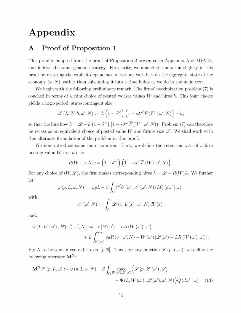
Appendix

A Proof of Proposition 1

This proof is adapted from the proof of Proposition 2 presented in Appendix A of MPV13,

and follows the same general strategy. For clarity, we amend the notation slightly in this

proof by restoring the explicit dependence of various variables on the aggregate state of the

economy (ω,N), rather than subsuming it into a time index as we do in the main text.

We begin with the following preliminary remark. The firms’ maximization problem (7) is

couched in terms of a joint choice of posted worker values W and hires h. This joint choice

yields a next-period, state-contingent size:

L (L,W, h, ω′, N) := L(1− δω

′)(

1− sλω′F (W | ω′, N)

)+ h,

so that the hire flow h = L −L(1− δω

′) (1− sλω′

F (W | ω′, N)). Problem (7) can therefore

be recast as an equivalent choice of posted value W and future size L . We shall work with

this alternate formulation of the problem in this proof.

We now introduce some more notation. First, we define the retention rate of a firm

posting value W in state ω:

R(W | ω,N) :=(1− δω

′)(

1− sλω′F (W | ω′, N)

).

For any choice of (W,L ), the firm makes corresponding hires h = L −R(W )L. We further

let:

φ (p, L, ω,N) := ωpL+ β

∫Ω

δω′U (ω′,N (ω′, N))LQ (dω′ | ω) ,

with:

N (ω′, N) :=

∫ p

p

L (x, L (x) , ω′, N) dΓ (x) .

and:

Φ (L,W (ω′) ,L (ω′), ω′, N) := −c [L (ω′)− LR (W (ω′) |ω′)]

+ L

∫ +∞

W (ω′)

vdR (v | ω′, N)−W (ω′) [L (ω′)− LR (W (ω′) |ω′)] .

Fix N to be some given c.d.f. over[p, p

]. Then, for any function S (p, L, ω), we define the

following operator MN:

MNS (p, L, ω) := φ (p, L, ω,N) + β

∫Ω

maxW (ω′),L (ω′)

⟨S [p,L (ω′) , ω′]

+ Φ (L,W (ω′) ,L (ω′), ω′, N)⟩Q (dω′ | ω) . (13)

34

Importantly, as stated in the proposition, we make the following two assumptions: first,

the sampling c.d.f. F (W ) is everywhere differentiable. This implies differentiability of R(W ).

Second, the hiring cost function is such that ε(c′) := hc′′(h)/c′(h) ≥ 1 for all h ≥ 0.

We then start the proof with the following lemma:

Lemma 1 Let S (p, L, ω) be bounded, continuous in p and L, increasing and convex in L,

and with increasing differences in (p, L) over(p, p

)× (0, 1). Then:

1. MNS is bounded and continuous in p and L;

2. There exists a measurable selection (V (p, L, ω,N) ,L (p, L, ω,N)) from the maximiz-

ing correspondence associated with MNS ;

3. Any such measurable selection is such that V and L are both increasing in p and L;

4. MNS is increasing and convex in L, and has increasing differences in (p, L) over(p, p

)× (0, 1).

Proof. In this proof, wherever possible without causing confusion, we will make

the dependence of all functions on aggregate state variables ω and N implicit to

streamline the notation.

Points 1 and 2 of this proposition follow immediately from the same arguments

as in the proof of Lemma 1 in MPV13, Appendix A. We now turn to the proof

of point 3. In each future state ω′, the firm solves:

maxW,L

⟨S (p,L ) + Φ (L,W,L )⟩ , (14)

where the dependence on ω′ and N of the various functions involved was kept

implicit to lighten notation. The FOC for W is:

0 = c′ [L − LR(W )]× LR′(W )− [L − LR(W )] (15)

and that for L is:

SL,r(p,L )−W−c′ [L − LR(W )] ≤ 0 ≤ SL,ℓ(p,L )−W−c′ [L − LR(W )] (16)

where SL,r and SL,ℓ denote the right- and left-derivatives of S w.r.t. L, which

exist everywhere by convexity of S .

Equation (16) implies that, at an optimal choice of L , SL,r(p,L ) ≤ SL,ℓ(p,L ).

But convexity of S implies that the converse inequality also holds, which proves

35

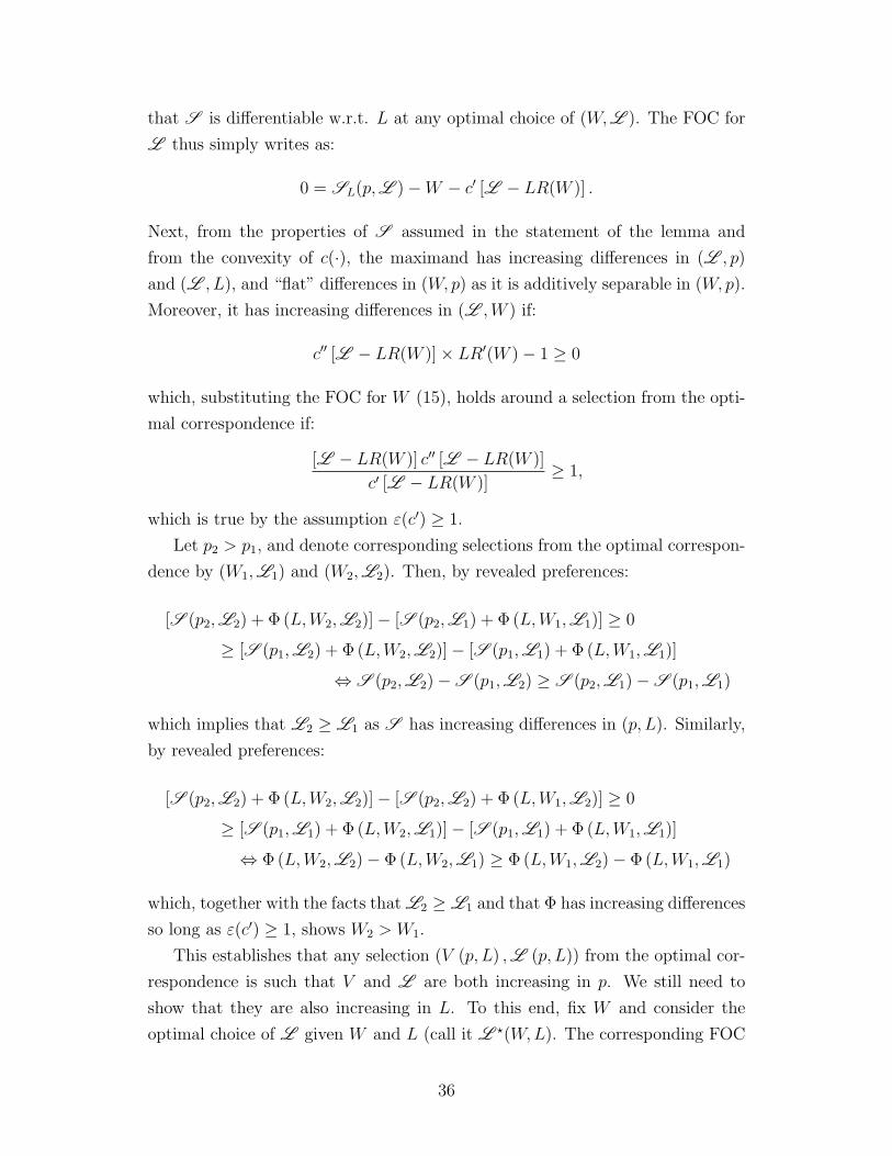
that S is differentiable w.r.t. L at any optimal choice of (W,L ). The FOC for

L thus simply writes as:

0 = SL(p,L )−W − c′ [L − LR(W )] .

Next, from the properties of S assumed in the statement of the lemma and

from the convexity of c(·), the maximand has increasing differences in (L , p)

and (L , L), and “flat” differences in (W, p) as it is additively separable in (W, p).

Moreover, it has increasing differences in (L ,W ) if:

c′′ [L − LR(W )]× LR′(W )− 1 ≥ 0

which, substituting the FOC for W (15), holds around a selection from the opti-

mal correspondence if:

[L − LR(W )] c′′ [L − LR(W )]

c′ [L − LR(W )]≥ 1,

which is true by the assumption ε(c′) ≥ 1.

Let p2 > p1, and denote corresponding selections from the optimal correspon-

dence by (W1,L1) and (W2,L2). Then, by revealed preferences:

[S (p2,L2) + Φ (L,W2,L2)]− [S (p2,L1) + Φ (L,W1,L1)] ≥ 0

≥ [S (p1,L2) + Φ (L,W2,L2)]− [S (p1,L1) + Φ (L,W1,L1)]

⇔ S (p2,L2)− S (p1,L2) ≥ S (p2,L1)− S (p1,L1)

which implies that L2 ≥ L1 as S has increasing differences in (p, L). Similarly,

by revealed preferences:

[S (p2,L2) + Φ (L,W2,L2)]− [S (p2,L2) + Φ (L,W1,L2)] ≥ 0

≥ [S (p1,L1) + Φ (L,W2,L1)]− [S (p1,L1) + Φ (L,W1,L1)]

⇔ Φ (L,W2,L2)− Φ (L,W2,L1) ≥ Φ (L,W1,L2)− Φ (L,W1,L1)

which, together with the facts that L2 ≥ L1 and that Φ has increasing differences

so long as ε(c′) ≥ 1, shows W2 > W1.

This establishes that any selection (V (p, L) ,L (p, L)) from the optimal cor-

respondence is such that V and L are both increasing in p. We still need to

show that they are also increasing in L. To this end, fix W and consider the

optimal choice of L given W and L (call it L ⋆(W,L). The corresponding FOC

36

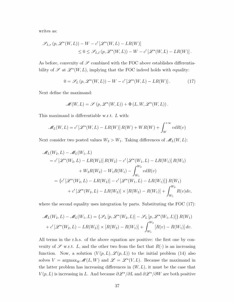
writes as:

SL,r (p,L⋆(W,L))−W − c′ [L ⋆(W,L)− LR(W )]

≤ 0 ≤ SL,ℓ (p,L⋆(W,L))−W − c′ [L ⋆(W,L)− LR(W )] .

As before, convexity of S combined with the FOC above establishes differentia-

bility of S at L ⋆(W,L), implying that the FOC indeed holds with equality:

0 = SL (p,L⋆(W,L))−W − c′ [L ⋆(W,L)− LR(W )] . (17)

Next define the maximand:

M (W,L) = S (p,L ⋆(W,L)) + Φ (L,W,L ⋆(W,L)) .

This maximand is differentiable w.r.t. L with:

ML(W,L) = c′ [L ⋆(W,L)− LR(W )]R(W ) +WR(W ) +

∫ +∞

W

vdR(v)

Next consider two posted values W2 > W1. Taking differences of ML(W,L):

ML(W2, L)− ML(W1, L)

= c′ [L ⋆(W2, L)− LR(W2)]R(W2)− c′ [L ⋆(W1, L)− LR(W1)]R(W1)

+W2R(W2)−W1R(W1)−∫ W2

W1

vdR(v)

= c′ [L ⋆(W2, L)− LR(W2)]− c′ [L ⋆(W1, L)− LR(W1)]R(W1)

+ c′ [L ⋆(W2, L)− LR(W2)]× [R(W2)−R(W1)] +

∫ W2

W1

R(v)dv,

where the second equality uses integration by parts. Substituting the FOC (17):

ML(W2, L)− ML(W1, L) = SL [p,L⋆(W2, L)]− SL [p,L

⋆(W1, L)]R(W1)

+ c′ [L ⋆(W2, L)− LR(W2)]× [R(W2)−R(W1)] +

∫ W2

W1

[R(v)−R(W1)] dv.

All terms in the r.h.s. of the above equation are positive: the first one by con-

vexity of S w.r.t. L, and the other two from the fact that R(·) is an increasing

function. Now, a solution (V (p, L),L (p, L)) to the initial problem (14) also

solves V = argmaxWM (L,W ) and L = L ⋆(V, L). Because the maximand in

the latter problem has increasing differences in (W,L), it must be the case that

V (p, L) is increasing in L. And because ∂L ⋆/∂L and ∂L ⋆/∂W are both positive

37

(provided that ε(c′) ≥ 1), it must be the case that L (p, L) = L ⋆ (V (p, L), L) is

also increasing in L.

Now on to point 4. Inspection of (13), in combination with the fact that

S is differentiable w.r.t. L at any optimal solution, shows that MNS is in

fact differentiable w.r.t. L (a stronger property than claimed in the lemma).

Furthermore:

∂

∂LMNS (p, L, ω) = ωp+ β

∫Ω

δω′U (ω′)Q (dω′ | ω)

+ β

∫Ω

c′ [L (p, L, ω′)− LR (V (p, L, ω′)|ω′)]R (V (p, L, ω′)|ω′)

+

∫ +∞

V (p,L,ω′)

vdR (v | ω′) + V (p, L, ω′)R (V (p, L, ω′)|ω′)

Q (dω′ | ω) (18)

This latter equation readily shows that MNS is increasing in L.

What is left is for us to establish that MNS is convex w.r.t. L and has

increasing differences in (L, p). To this end, first note that substitution of the

FOC (16) into (18) yields an alternative expression for ∂MNS /∂L:

∂

∂LMNS (p, L, ω) = ωp+ β

∫Ω

δω′U (ω′)Q (dω′ | ω)

+β

∫Ω

SL (p,L (p, L, ω′))×R (V (p, L, ω′)|ω′)+

∫ +∞

V (p,L,ω′)

vdR (v | ω′)

Q (dω′ | ω)

Now take L2 > L1:

∂

∂LMNS (p, L2, ω)−

∂

∂LMNS (p, L1, ω)

= β

∫Ω

SL (p,L (p, L2, ω

′))×R (V (p, L2, ω′)|ω′)

−SL (p,L (p, L1, ω′))×R (V (p, L1, ω

′)|ω′)−∫ V (p,L2,ω′)

V (p,L1,ω′)

vdR (v | ω′)

Q (dω′ | ω)

= β

∫Ω

[SL (p,L (p, L2, ω

′))− SL (p,L (p, L1, ω′))]×R (V (p, L1, ω

′)|ω′)

+

∫ V (p,L2,ω′)

V (p,L1,ω′)

[SL (p,L (p, L2, ω′))− v] dR (v | ω′)

Q (dω′ | ω)

which is positive, by convexity of S , the fact that both V and L are increasing

in L, and the fact that SL (p,L (p, L2, ω′)) ≥ V (p, L2, ω

′). This establishes

38

convexity of MNS w.r.t. L. Increasing differences in (L, p) is follows from

similar steps (only taking differences in p of ∂MNS /∂L), so we omit the details.

Now consider the set of functions defined over[p, p

]× [0, 1] × Ω that are continuous in

(p, L) and call it C[p,p]×[0,1]×Ω. That set is a Banach space when endowed with the sup norm.

As Lemma 1 suggests we will be interested in the properties of a subset C ′[p,p]×[0,1]×Ω

⊂C[p,p]×[0,1]×Ω of functions that are increasing and convex in L and have increasing differences

in (p, L). We next state two ancillary lemmas, which will establish as a corollary (Corollary

1) that C ′[p,p]×[0,1]×Ω

is closed in C[p,p]×[0,1]×Ω under the sup norm.

Lemma 2 Let X be an interval in R and fn : X → R, N ∈ N such that fn converges

uniformly to f . Then:

1. if fn is nondecreasing for all n, so is f ;

2. if fn is convex for all n, so is f .

Proof. See the appendix of MPV13.

Lemma 3 Let X ⊂ R2 be a convex set and fn : X → R, N ∈ N be functions with increasing

differences such that fn converges uniformly to f . Then f has increasing differences.

Proof. See the appendix of MPV13.

Corollary 1 The set C ′[p,p]×[0,1]×Ω

of functions defined over[p, p

]×[0, 1]×Ω that are increas-

ing and convex in L and have increasing differences in (p, L) is a closed subset of C[p,p]×[0,1]×Ω

under the sup norm.

The latter corollary establishes that, given a fixed N , the functions that are relevant to

Lemma 1 live in a closed subset of a Banach space of functions under the sup norm. The

following lemma shows that the operator considered in Lemma 1 is a contraction under that

same norm.

Lemma 4 The operator MN defined in (13) maps C ′[p,p]×[0,1]×Ω

into itself and is a contrac-

tion of modulus β under the sup norm.

Proof. That MN maps C ′[p,p]×[0,1]×Ω

into itself flows directly from part of the

proof of Lemma 1. To prove that MN is a contraction, we can easily check using

(13) that MN satisfies Blackwell’s sufficient conditions with modulus β.

39

We are now in a position to prove the proposition. Given the initially fixed N , the

operator MN, which by Lemma 4 is a contraction from C[p,p]×[0,1]×Ω into itself, and has

a unique fixed point SN in that set (by the Contraction Mapping Theorem). Moreover,

since C ′[p,p]×[0,1]×Ω

is a closed subset of C[p,p]×[0,1]×Ω (Lemma 2) and since MN also maps

C ′[p,p]×[0,1]×Ω

into itself (Lemma 1), that fixed point SN belongs to C ′[p,p]×[0,1]×Ω

.

Summing up, what we have established thus far is that for any fixed N ∈ C[p,p], the

operator MN over functions of (p, L, ω) has a unique, bounded and continuous fixed point

S ⋆N = MNS ⋆

N ∈ C ′[p,p]×[0,1]×Ω

⊂ C[p,p]×[0,1]×Ω.

We finally turn to the Bellman operator M which is relevant to the firm’s problem. That

operator M applies to functions S defined on[p, p

]× [0, 1]×Ω×C[p,p] and is defined as the

following “extension” of MN:

MS (p, L, ω,N) := φ (p, L, ω,N) + β

∫Ω

maxW (ω′),L (ω′)

⟨S [p,L (ω′) , ω′]

+ Φ (L,W (ω′) ,L (ω′), ω′, N)⟩Q (dω′ | ω) .

If an equilibrium exists, then a firm has a best response and a value S which solves S = MS.

For every N ∈ C[p,p], by definition of M and MN this implies S = MNS. Since the fixed

point of MN is unique, if S = MS exists then for every fixed N ∈ C[p,p] we have for all

(p, L, ω) ∈[p, p

]× [0, 1] × Ω: S (p, L, ω,N) = S ⋆

N (p, L, ω). Therefore, if the value function

S and an equilibrium of the contract-posting game exist, then S ∈ C ′[p,p]×[0,1]×Ω

: the typical

firm’s value function is continuous in p and L, increasing and convex in L and has increasing

differences in (p, L). By the same standard comparative statics arguments that we invoked

in the proof of Lemma 1, the maximizing correspondence is increasing in p and L in the

strong set sense, hence all of its measurable selections are weakly increasing in p and L.

B The computation algorithm

We describe the algorithm that we use to approximate numerically RPE contracts. We start

with the case of exogenous vacancies and hiring for notational simplicity, and return to the

general case of endogenous hiring at the end.

B.1 RPE Dynamics

With exogenous and uniform sampling weights, in any RPE, aggregate ads and sampling

distribution are At(ω) = 1, Ft(p) = Γ (p), the job finding and vacancy filling rates are:

λ(ωt, Nt−1) = m

(1,

1

1−Nt−1(p) + s (1− δ(ωt))Nt−1(p)

)(19)

40

η(ωt, Nt−1) = m (1−Nt−1(p) + s (1− δ(ωt))Nt−1(p), 1)

The law of motion of firm-level employment is:

L(p|ωt, Nt−1)

= Nt−1(p) (1− δ(ωt))[1− sλ(ωt, Nt−1)Γ(p)

]+ η (ωt, Nt−1)

1−Nt−1(p) + s (1− δ(ωt))Nt−1(p)

1−Nt−1(p) + s (1− δ(ωt))Nt−1(p)

= Nt−1(p) (1− δ(ωt))[1− sλ(ωt, Nt−1)Γ(p)

]+ λ (ωt, Nt−1) [1−Nt−1(p) + s (1− δ(ωt))Nt−1(p)]

Consequently, the employment distribution evolves according to

N (p|ωt, Nt−1) =

∫ p

p

L(x|ωt, Nt−1)dΓ (x)

= (1− δ(ωt))

∫ p

p

Nt−1(x) [1 + sλ(ωt, Nt−1)Γ(x)] dΓ (x) + λ(ωt, Nt−1) [1−Nt−1(p)] Γ (p)

(20)

We look for contracts that support this RPE allocation. That is, if all firms follow RPE

strategies, so that the above dynamics apply, we look for the value that each firm p offers as

a best-response.

B.2 Euler equation

Let V (p|ωt, Nt−1) be the optimal policy given aggregate states ωt, Nt−1, U(ωt, Nt−1) the value

of unemployment, µ(p|ωt, Nt−1) the shadow marginal value of one more worker. Then using

the Bellman equation of the unemployed worker

U(ωt, Nt−1) = b (ωt) + βEωt+1|ωt

U (ωt+1,N (·|ωt, Nt−1)) + λ (ωt+1,N (·|ωt, Nt−1))

×∫ p

p

max ⟨V (x|ωt+1,N (·|ωt, Nt−1))− U (ωt+1,N (·|ωt, Nt−1)) , 0⟩ dΓ (x)

the FOC for an optimal offered value can be written as

V (p|ωt, Nt−1)− U(ωt, Nt−1) =

∫ p

p

[µ(x|ωt, Nt−1)− U(ωt, Nt−1)] s (1− δ(ωt)) dNt−1(x)

1−Nt−1(p) + s (1− δ(ωt))Nt−1(p)

41

and the Euler equation as

µ(p|ωt, Nt−1)− U(ωt, Nt−1) = ωtp− b(ωt)

+ βEωt+1|ωt

(1− δ(ωt+1))

[1− sλ (ωt+1,N (·|ωt, Nt−1)) Γ(p)

]× [µ (p|ωt+1,N (·|ωt, Nt−1))− U (ωt+1,N (·|ωt, Nt−1))]

+(1− δ(ωt+1)) sλ (ωt+1,N (·|ωt, Nt−1)

∫ p

p

[V (x|ωt+1,N (·|ωt, Nt−1))− U (ωt+1,N (·|ωt, Nt−1))] dΓ (x)

− λ (ωt+1,N (·|ωt, Nt−1)

∫ p

p

[V (x|ωt+1,N (·|ωt, Nt−1))− U (ωt+1,N (·|ωt, Nt−1))] dΓ (x)

Let

σ(p|ωt, Nt−1) := µ(p|ωt, Nt−1)− U(ωt, Nt−1)

so that

V (p|ωt+1,N (·|ωt, Nt−1))− U (ωt+1,N (·|ωt, Nt−1))

= s (1− δ(ωt+1))

∫ p

p

σ (x|ωt+1,N (·|ωt, Nt−1))

1−N (p|ωt, Nt−1) + s (1− δ(ωt+1))N (p|ωt, Nt−1)dN (x|ωt, Nt−1)

Substituting in, σ(p|ωt, Nt−1) solves the Euler equation

σ(p|ωt, Nt−1) = ωtp− b(ωt)

+ βEωt+1|ωt

(1− δ(ωt+1))

[1− sλ(ωt+1,N (·|ωt, Nt−1))Γ(p)

]σ (p|ωt+1,N (·|ωt, Nt−1))

+(1− δ(ωt+1))2 s2λ (ωt+1,N (·|ωt, Nt−1))

∫ p

p

∫ x

p

σ (y|ωt+1,N (·|ωt, Nt−1)) dN (y|ωt, Nt−1)dΓ (x)

1−N (p|ωt, Nt−1) + s (1− δ(ωt+1))N (p|ωt, Nt−1)

−(1− δ(ωt+1)) sλ (ωt+1,N (·|ωt, Nt−1))

∫ p

p

∫ x

p

σ (y|ωt+1,N (·|ωt, Nt−1)) dN (y|ωt, Nt−1)dΓ (x)

1−N (p|ωt, Nt−1) + s (1− δ(ωt+1))N (p|ωt, Nt−1)

(21)

where λ(p|ωt, Nt−1) and N (p|ωt, Nt−1) were defined before in (19) and (20).

B.3 Computation

Fix a large T > 0, draw a history of aggregate shocks ω⋆ = ω⋆t

Tt=1 and compute the associ-

ated N⋆ = N⋆t

Tt=1 from N⋆

t = N(p|ωt, N

⋆t−1

). We want to compute, at least approximately,

the realized path of

σ(p|ω⋆

t , N⋆t−1

):= σ⋆

t (p)

42

where the dependence on N⋆t−1 is encoded in the subscript t of σ⋆

t . From this sequence of

functions of p we can compute offered values (and adverts in the endogenous vacancy case

addressed below). In order to compute these values, we can apply the Euler equation (21)

to(ω⋆t , N

⋆t−1

):

σ(p|ω⋆

t , N⋆t−1

)= ω⋆

t p− b (ω⋆t )

+ βEωt+1|ω⋆t

(1− δ(ωt+1))

[1− sλ (ωt+1, N

⋆t ) Γ(p)

]σ (p|ωt+1, N

⋆t )

+ (1− δ(ωt+1))2 s2λ (ωt+1, N

⋆t )

∫ p

p

∫ x

p

σ (y|ωt+1, N⋆t ) dN

⋆t (y)dΓ(x)

1−N⋆t (p) + s (1− δ(ωt+1))N⋆

t (p)

− (1− δ(ωt+1)) sλ (ωt+1, N⋆t )

∫ p

p

∫ x

p

σ (y|ωt+1, N⋆t ) dN

⋆t (y)dΓ(x)

1−N⋆t (p) + s (1− δ(ωt+1))N⋆

t (p)

(22)

To compute the r.h.s. we need to compute σ (y|ωt+1, N⋆t ) for every y and every ωt+1. To do

so, we apply again (21) to N⋆t−1 and any possible value of ωt

σ(p|ωt, N

⋆t−1

)= ωtp− b(ωt)

+ βEωt+1|ωt

(1− δ(ωt+1))

[1− sλ

(ωt+1,N

(·|ωt, N

⋆t−1

))Γ(p)

]σ(p|ωt+1,N

(·|ωt, N

⋆t−1

))+(1− δ(ωt+1))

2 s2λ(ωt+1,N

(·|ωt, N

⋆t−1

)) ∫ p

p

∫ x

p

σ(y|ωt+1,N

(·|ωt, N

⋆t−1

))dN

(y|ωt, N

⋆t−1

)dΓ(x)

1−N(p|ωt, N⋆

t−1

)+ s (1− δ(ωt+1))N

(p|ωt, N⋆

t−1

)−(1− δ(ωt+1)) sλ

(ωt+1,N

(·|ωt, N

⋆t−1

)) ∫ p

p

∫ x

p

σ(y|ωt+1,N

(·|ωt, N

⋆t−1

))dN

(y|ωt, N

⋆t−1

)dΓ(x)

1−N(p|ωt, N⋆

t−1

)+ s (1− δ(ωt+1))N

(p|ωt, N⋆

t−1

)

To compute the r.h.s. we need to compute N(·|ωt, N

⋆t−1

)for each ωt, which is feasible, and

σ(y|ωt+1,N

(·|ωt, N

⋆t−1

))for every value of N

(·|ωt, N

⋆t−1

). For that, it is sufficient (but not

necessary) to know the entire map σ (y|ωt+1, Nt) for every (ωt+1, Nt), which is infeasible,

because Nt is infinite-dimensional.

B.4 An “anticipatory” approximation

In σ (y|ωt+1, Nt), we approximate everyNt which could have been generated byN(·|ωt, N

⋆t−1

)depending on the realization of ωt with the N⋆

t = N(·|ω⋆

t , N⋆t−1

)realized on this RPE

path. In so doing, we effectively reset the dimensionality of each firm’s state space to the

cardinality of Ω (the support of ω) in every period. Starting from a terminal condition

σ (p|ωT+1, N⋆T ) = ωT+1p− b(ωT+1), we compute recursively the approximation σ (y|ωt+1, N

⋆t )

43

back in time t = T, T − 1, · · · , 0 using:

σ(p|ωt, N

⋆t−1

)= ωtp− b(ωt)

+ βEωt+1|ωt

(1− δ(ωt+1))

[1− sλ

(ωt+1,N

(·|ωt, N

⋆t−1

))Γ(p)

]σ(p|ωt+1,N

(·|ωt, N

⋆t−1

))+(1− δ(ωt+1))

2 s2λ(ωt+1,N

(·|ωt, N

⋆t−1

)) ∫ p

p

∫ x

p

σ (y|ωt+1, N⋆t ) dN

(y|ωt, N

⋆t−1

)dΓ(x)

1−N(p|ωt, N⋆

t−1

)+ s (1− δ(ωt+1))N

(p|ωt, N⋆

t−1

)−(1− δ(ωt+1)) sλ

(ωt+1,N

(·|ωt, N

⋆t−1

)) ∫ p

p

∫ x

p

σ (y|ωt+1, N⋆t ) dN

(y|ωt, N

⋆t−1

)dΓ(x)

1−N(p|ωt, N⋆

t−1

)+ s (1− δ(ωt+1))N

(p|ωt, N⋆

t−1

)We then truncate the last part of the history as a ‘burn-in’ period, and approximate the

desired σ(p|ω⋆

t , N⋆t−1

):= σ⋆

t (p) with σ(p|ω⋆

t , N⋆t−1

), the function just obtained evaluated on

the realized path.

Conceptually, in this approximation, a firm still views aggregate productivity ωt as ran-

dom at the beginning of period t and takes conditional expectations w.r.t. this random vari-

able, but evaluates the future marginal value of a new employee as if the period-t realized

employment distribution (N(·|ωt, N

⋆t−1

)) were always the one occurring on the equilibrium

path (N⋆t = N

(·|ω⋆

t , N⋆t−1

)), regardless of ωt. Since Nt is a slow-moving object, the deviation

supp,ω

∣∣N⋆t (p)−N

(p|ω,N⋆

t−1

)∣∣is likely to be small one period ahead, and the quality of the approximation rests on the

continuity of the functional σ(p|ωt+1, ·). For all other purposes, such as taking expectations

across firms, the firm uses the correct period-t employment distribution N(·|ωt, N

⋆t−1

)that

occurs in each aggregate state.

The next step would be to compute recursively σ(p|ωt,N

(·|ωt−1, N

⋆t−2

)), a function

of p, time t, ωt−1 and ωt. More generally, we can compute recursively the “kth-order”

approximation

σ(p|ωt,N

(·|ωt−1,N

(·|ωt−2, · · · N

(·|ωt−k+1, N

⋆t−k

))))a function of p, time t, ωt−k+1, · · · , ωt+1. Keeping track of the entire history, k = ∞, yields

the exact optimal policy. Each time k is increased by one, the dimension of the state space

that one must keep track of is multiplied by the number of support points in the distribution

of ω (the cardinality of Ω). Hence, our algorithm sets k = 1.

B.5 Endogenous hiring

We return to the full model, where hiring and sampling weights are endogenous. The algo-

rithm for this case, which is how we obtain the results presented in the paper,18 is analogous

18The code is available from https://sites.google.com/site/fabienpostelvinay/working-papers

44

to the case of exogenous sampling weights, but requires an additional iteration.

We start by guessing an arbitrary non-negative candidate profile of ad postings a(0)t (p, ω)

for t = 1, 2, · · · , T and ω ∈ Ω. Then at step n = 0, 1, 2, · · · we proceed as follows. Given the

current a(n)t (p, ω) for t = 1, 2, · · · , T we evaluate a

(n)t (p, ω) at ω = ωs

t tar to obtain a path

of sampling weights a(n)t (p, ω⋆

t ). Then, given an initial distribution of employment N⋆1 (·),

we compute the resulting contact rates(λ⋆(n)t , η

⋆(n)t

)and employment distributions N

⋆(n)t (·).

We then apply the previous algorithm to obtain an estimated path σ(n)(p|ωt, N

⋆(n)t−1

). Next,

we use the FOC (11) for optimal hiring: c′(H

(n)t

(p|ω,N⋆(n)

t−1

))= σ(n)

(p|ω,N⋆(n)

t−1

)to obtain

an estimate of the hiring path H(n)t

(·|ω,N⋆(n)

t−1

). Finally, we update the path of job ads

to a(n+1)t (p, ω) using H

(n)t

(p|ω,N⋆(n)

t−1

)and the relationship between ads input and hiring

output, with the contact rate and acceptance probability evaluated at the ‘starred’ RPE

H(n)t

(p|ω,N⋆(n)

t−1

)= a

(n+1)t (p, ω)η

⋆(n)t P

(n)t

(p|ω,N⋆(n)

t−1

)(23)

where the probability that the offer is accepted in RPE can be computed beforehand, along

with the turnover rates and employment distribution:

P(n)t

(p|ω,N⋆(n)

t−1

)=

1−N⋆(n)t−1 (p) + s (1− δ(ω))N

⋆(n)t−1 (p)

1−N⋆(n)t−1 (p) + s (1− δ(ω))N

⋆(n)t−1 (p)

(24)

We then raise n by one, and iterate, until convergence at some n′ of a(n)t (p, ω) within some

small tolerance for all t, p, and ω. Then an′

t (p, ω⋆t ) provides an ‘anticipatory’ approximation

to the true ad-posting function a⋆t (p) = a(p|ω⋆

t , N⋆t−1

)in the same way that σn′ (

p|ω⋆t , N

⋆t−1

)approximates σ⋆

t (p).

B.6 Approximation diagnostics

Our approximation to the RPE is predicated on the conjecture that σ(p|ωt+1,N

(·|ωt, N

⋆t−1

))is close to σ (p|ωt+1, N

⋆t ) = σ

(p|ωt+1,N

(·|ω⋆

t , N⋆t−1

))for every value of ωt other than the ω⋆

t

that occurs on the equilibrium path. This will be the case in particular if N moves slowly

over time and if σ (p|ω,N) is much less responsive to N than it is to ω.

After computing our proposed RPE, a natural candidate for the desired σ (p|ωt+1, Nt) is

σ(p|ω⋆

s , N⋆s−1

)for some time s, if any, when the state ω⋆

s = ωt+1 and N⋆s−1 is close to Nt

in the sup norm. We perform the following check on our candidate RPE. For every t, we

select the time periods s such that ω⋆s = ωt+1; with a state space Ω that takes 20 values,

recurrence of ω is frequent and we can find many such times s. At each time s in this

set, we average σ(p|ω⋆

s , N⋆s−1

)over p using the firm measure Γ. Finally, we study the time

series variation of this average over the set of times s, and we find that it is minor, never

45

exceeding 5% in relative terms, and often less. Conversely, the variation over times s′ when

N⋆s′−1 remains approximately the same, but ω⋆

s′ varies, can be as large as 70%. Therefore

in our approximate equilibrium, σ(p|ω⋆

t , N⋆t−1

)is much more sensitive to changes in its first

argument, and indeed almost insensitive to changes in its second argument, conditional on

the same value of the first.

46