Department of Economics University of Bristol 8 Woodland Road Bristol BS8 1TN United Kingdom

LABOUR INFORMALITY, SELECTIVE

MIGRATION, AND PRODUCTIVITY IN GENERAL EQUILIBRIUM

Huikang Ying

Discussion Paper 15 / 653

2 April 2015

Labour Informality, Selective Migration, andProductivity in General Equilibrium ∗

Huikang Ying†

University of Bristol

March 31, 2015

Abstract

This paper studies the interactions between urban labour infor-mality and selective migration, and explores the consequences ofproductivity changes at both sectoral and individual levels. It pro-poses a general equilibrium model with heterogeneous workers tocharacterize the sizable agriculture sector and urban informality indeveloping economies, and discusses implications for wages and in-equality. The model links the size of the urban informal sector to thedistributions of individual productivity endowments. The findingsuggests that improving average individual skills is an efficient wayto alleviate urban underemployment. Equilibrium responses also in-dicate that changes in labour markets have only modest effects onwages and inequality.JEL Categories: J24, O15, O17Keywords: Rural-urban migration, informal sector, productivity changes,wage inequality

∗Preliminary. I am grateful to Jonathan Temple for his useful guidance and comments.The usual disclaimer applies.

†Department of Economics, University of Bristol, 8 Woodland Road, Bristol, BS8 1TN.Email: huikang.ying@bristol.ac.uk.

1 Introduction

This paper studies the interactions between urban labour informality andselective migration in developing countries, and explores the consequencesof sectoral and individual productivity changes for the labour market andinequality. Existing studies, such as Moene (1988), Zenou (2008, 2011)and Satchi and Temple (2009), have investigated the link between labourmarkets and rural-urban migration from different perspectives and dis-cussed policy implications. However, the current literature often tends tooverlook the crucial role of labour heterogeneity. As a consequence, wehave known little about how different distributions of individual produc-tivity affect urban labour markets, and how these effects relate to selectivemigration of heterogeneous workers. Moreover, implications for wage dis-tributions and inequality dynamics are absent when workers are assumedto be identical.

To complement the existing literature, this paper develops a generalequilibrium model with heterogeneous workers to characterize the typi-cal economic structure in developing countries. In the modelled economy,there coexists a large rural sector producing agricultural goods and anurban sector with formal manufacturing and an informal sector in whichworkers are self-employed. Workers choose their occupations followinga Roy-type mechanism. Endowed with different productivity levels inagriculture and non-agriculture, workers will select the sector where theyobtain higher expected lifetime utility. Workers in the non-agriculture sec-tor face the risk of unemployment due to matching frictions in the ur-ban labour market. When their matches with firms are destroyed, urbanworkers can either be self-employed in the informal sector, or move to theagriculture sector.

I calibrate the model to match the economic structure of Malawi, aneconomy with a large scale of agricultural production and an urban infor-mal sector. The steady-state equilibrium of the model is consistent withthis economic structure, without assuming unrealistic high recruitmentcosts, or implying a long duration of job vacancies. Furthermore, giventhat workers are heterogeneous in productivity, the model is more flexiblein explaining the size of the informal sector than those assuming homo-geneous workers. It links urban employment to the distributions of indi-

1

vidual productivity endowments, and gives rise to the policy implicationthat improving average labour productivity, even when causing some ex-tent of skill divergence across workers, can significantly ameliorate urbanunderemployment.

The equilibrium has rich implications for wage distributions and in-equality. Wages in the model are endogenously determined by the labourcompositions across sectors via the selective migration of heterogeneousworkers. In the baseline calibration, the wage gap between the two sec-tors is the result of self-selection: most workers, including those with lowproductivity, are working in the agriculture sector at the early stage of eco-nomic development, whereas only those with relatively high skills are incities. The (relative) inequality within each sector is determined by the dis-parity of productivity of workers in the sector. Inequality levels are alwayslower in agriculture than non-agriculture, as rural workers are generallyendowed with low productivity in the calibrated model.

The experiments for equilibrium responses show that changes of sec-toral and individual productivity will have significant influences on theurban labour market, sectoral employment shares and wage inequality.In contrast, changes in structural parameters of the labour market haveonly modest effects on wages and inequality. Therefore, policies aiming atinequality reduction probably need to look beyond the labour market.

The remainder of the paper will proceed as follows. Section 2 discussesthe literature relating to this paper. Section 3 lays out the model and dis-cusses the steady-state equilibrium. Section 4 calibrates the model to dataand presents the baseline equilibrium outcomes. Equilibrium responseswill be examined in section 5. Section 6 concludes.

2 Relation to existing literature

As noted in the introduction, a distinct feature of this paper is to modellabour markets for developing economies with ex ante heterogeneous work-ers. My approach is closely linked to two recent papers.

The first one is Lagakos and Waugh (2013), who formulate the occu-pational selection mechanism of Roy (1951) in a dual economy. In theirmodel, workers have separate skills in agriculture and non-agriculture,and they choose the sector that maximizes their wages based on their

2

productivity endowments. The mechanism determines the rural-urbanlabour compositions, as well as sectoral productivity in equilibrium. Thisframework is useful in studying various issues for dual economies, such ascross-country differences in labour productivity (e.g. Lagakos and Waugh,2013; Kuralbayeva and Stefanski, 2013), the rural-urban gap and migration(Young, 2013), and the dynamics of wages, inequality and poverty (Templeand Ying, 2014; Ying, 2014).

Secondly, the model draws from the work of Albrecht, Navarro andVroman (2009) in terms of modelling heterogeneity in labour markets. Al-brecht et al. extend the search and matching model of Mortensen andPissarides (1994, 1999) to allow an informal sector and labour heterogene-ity, and study various labour market policies. In their model, productivityendowments of workers are characterized by a continuous distribution,and individuals could work for either the formal sector or the informalsector depending on their productivity levels, or they may be unemployeddue to matching frictions. Productivity heterogeneity in labour markets isalso discussed in papers such as Strand (1987), Amaral and Quintin (2006)and Pries (2008), among others, but their models only consider two typesof heterogeneous workers (i.e. low-productivity and high-productivityworkers), which gives rise to relatively limited implications, especially forwages and inequality in equilibrium.1

This paper simplifies Albrecht et al. (2009) with an exogenous job de-struction rate, and embeds it into the Lagakos-Waugh framework. So inthis model, workers will have an outside option when they are unem-ployed in cities, that is, the agriculture sector. And based on this, therelations between labour informality and selective migration can be ex-plored.

The paper also relates to the well-known Harris-Todaro model, whichwas first proposed to explain the persistence of rural-urban migrationin spite of high urban unemployment (Todaro, 1969; Harris and Todaro,1970). They argue that workers have incentives to locate in cities as longas the expected income in the urban sector is relatively high. Later stud-ies, such as Moene (1988), MacLeod and Malcomson (1998), Sato (2004),

1Another way to model sectoral wage distributions is to consider homogeneous work-ers but heterogeneous firms. A recent example is Meghir et al. (2015), who introduce anequilibrium wage-posting model based on Burdett and Mortensen (1998), in which hetero-geneous firms can choose an optimal sector.

3

Laing, Park and Wang (2005), Zenou (2008, 2011), and Satchi and Tem-ple (2009), among others, analyze models related to this framework anddiscuss various issues.

Among the list, this paper is especially close to Satchi and Temple(2009) regarding the model structure and the treatment of labour infor-mality. They recast the Harris-Todaro equilibrium in terms of a search andmatching framework for the urban sector, and explore the interactionsbetween labour markets and sectoral productivity levels for developingcountries. Their paper redefines urban unemployment as self-employmentin the informal sector, based on the fact that workers in poor countries can-not afford unemployment, and need work to maintain subsistence con-sumption. In this paper, I follow their treatment for simplicity, but themodel can be extended to allow for open unemployment, as in Zenou(2008), Albrecht et al. (2009) and Bosch and Esteban-Pretel (2012).

3 The model

There are two production sectors in the modelled economy: the rural (agri-culture) sector, denoted by a, and the urban (non-agriculture) sector, m.The economy is small and open, and thus outputs from the two sectorscan be exchanged on world markets at an exogenous relative price, p,where the non-agriculture good is the numéraire.

The two production sectors have different labour market structures.The agriculture sector is characterized as a full employment sector, whereasthe urban labour market has a non-Walrasian feature, where workers maybe unemployed due to search and matching frictions. Jobless urban work-ers have to be self-employed in the informal sector for subsistence con-sumption, and they keep looking for formal jobs while working informally.I will use the terms ‘self-employed’ and ‘unemployed’ interchangeably inthe remainder of this paper, since they represent the same state of an urbanworker.

Workers are modeled as a continuum with the population normalizedto unity, and each of them is endowed with distinct sectoral productivitylevels, denoted by a vector {za, zm}. Migration across the two productionsectors is costless, and thus workers always select the sector that optimizestheir lifetime utility. When workers choose the rural sector, their agricul-

4

tural productivity za is said to be ‘realized’ while zm becomes ‘latent’, andvice versa for those who are working in non-agriculture, either for the for-mal sector or the informal sector.

For simplicity, I assume linear production technologies for the agri-culture sector and the non-agriculture formal sector, with the exogenoussectoral total factor productivity levels (TFPs) xa and xm respectively. Sothe outputs of an employed worker in the two sectors are given by f (za) =

xaza and g (zm) = xmzm respectively.

3.1 The urban labour market

The urban labour market is characterized by a search and matching frame-work with exogenous job destruction and heterogeneous labour.2 Workersand firms will match if the joint surplus from the match exceeds the val-ues when they are unmatched. A number of urban workers, denoted byuLm, are unemployed, where u is the urban unemployment rate, also in-terpreted as the relative size of the informal sector, and Lm is the totallabour force in cities. The number of job vacancies offered by urban firmsis vLm. The nature of job matches is captured by the matching functionmLm = m (uLm, vLm).3 Define

q (θ) ≡ m (uLm, vLm)

vLm= m

(1θ

, 1)

where θ ≡ v/u is interpreted as the tightness of the labour market. Thematching process is assumed the same across all types of workers. Va-cancies are filled at the rate of q (θ), and unemployed workers will matchwith vacancies at the rate of θq (θ). q (θ) is decreasing in θ, while θq (θ) isincreasing in θ.

All workers are employable by firms.4 And regardless of their endow-ments of productivity, they will face the same exogenous job separationrate λ. Therefore, the flow balance condition in steady state is given bythe standard Beveridge curve

2Usual notations are applied as in Pissarides (2000).3The matching function has standard properties as in Pissarides (2000).4I will show later that no worker will be rejected due to low productivity, since the

value of a filled job is always non-negative.

5

λ (1− u) = θq (θ) u (1)

Since θq (θ) and λ are identical across workers, the unemployment ratein steady state will be the same for all workers, which further impliesthat the steady-state distributions of individual productivity should beidentical for both employed and unemployed workers in the urban sector.

In the formal sector, employed workers are offered a wage paymentwm (zm), depending on their non-agricultural productivity. When they areself-employed, they earn ζu for each unit of their productivity, and thuslabour income is given by ζuzm in the informal sector. Let W (zm) andU (zm) denote the expected values of income streams for workers with zm

productivity, when they are employed and self-employed respectively. TheBellman equations for W (zm) and U (zm) in steady state are given by

rW (zm) = wm (zm) + λ [U (zm)−W (zm)] (2)

rU (zm) = ζuzm + θq (θ) [W (zm)−U (zm)] (3)

where r is the real interest rate. Solving the above Bellman equationsyields

rW (zm) =λζuzm + [r + θq (θ)]wm (zm)

r + λ + θq (θ)

rU (zm) =(r + λ) ζuzm + θq (θ)wm (zm)

r + λ + θq (θ)(4)

The expected value of employment differs from labour income due tothe risk of potential unemployment. Workers prefer to stay in jobs as longas W (zm) ≥ U (zm), or wm (zm) ≥ ζuzm, and thus a sufficient condition,xm ≥ ζu is required.5

There are a large number of firms in the urban sector, and they hireworkers to make use of their productivity in non-agriculture. The produc-tion technology is such that heterogeneous workers are perfect substitutesat fixed ratios. Each firm offers one job vacancy that is open to all typesof workers. When the vacancy is unfilled, the discounted present value isgiven by

5See Pissarides (2000, p. 14, 18) for discussion.

6

rV = −c + q (θ) E max [J (zm)−V, 0] (5)

where the expectation is to be taken over the productivity distributionamong the unemployed workers, since firms are not able to observe work-ers’ productivity until they meet. But as the flow balance condition sug-gests, the productivity distribution of the unemployed workers is identicalto that of all urban workers in steady state.6

When the job vacancy is matched with a type zm worker, the assetvalue becomes

rJ (zm) = xmzm − wm (zm)− λJ (zm) (6)

Note that equation (6) makes use of the free-entry condition that rulesout any profit opportunity from opening new job vacancies, i.e. V = 0.

3.2 Wage determination and job creation

Wages are determined by Nash bargaining, which splits the match surplusbetween workers and firms, based on the parameter of workers’ bargain-ing power β ∈ (0, 1).

For each pair of worker and firm, the wage wm (zm) solves

maxwm(zm)

[W (zm)−U (zm)]β J (zm)

1−β

The first order condition of the bargaining problem leads to the stan-dard surplus sharing rule

(1− β) [W (zm)−U (zm)] = βJ (zm) (7)

Making use of equations (2) and (6), some algebra yields the rule forwage determination:

wm (zm) = βxmzm + (1− β) rU (zm) (8)

It suggests, as in Albrecht et al. (2009), that the wage of a worker is a

6Albrecht et al. (2009) use the same expression for the vacancy value, but they requiremore complicated expectations of productivity for unemployed workers, as they separateinformal employment from open unemployment.

7

weighted sum of his or her output in the formal sector and the expectedvalue of self-employment.7 Substituting rU (zm) from (4) yields

wm (zm) =β [(r + λ) + θq (θ)] xm + (1− β) (r + λ) ζu

r + λ + βθq (θ)· zm ≡ ζmzm (9)

where ζm denotes the payment to each unit of effective labour in the ur-ban formal sector. Equation (9) indicates that employed urban workers arepaid in proportion to their non-agricultural productivity levels in equi-librium, and the effective wage is independent of workers’ productivityendowments.8

The remaining question in the urban labour market is how matchesbetween workers and firms are formed under the rule for wage determi-nation. It is implied from the surplus sharing rule (7) that the value of anyfilled job J (zm) is always non-negative, given that W (zm) ≥ U (zm) holds.Therefore, all unemployed workers are employable. Equation (5) suggeststhat in equilibrium the expected value of meeting a worker is given by

E [J (zm)] =c

q (θ)(10)

Evaluating the expectation of J (zm) from equation (6), and combiningit with (10) yields the job creation condition

cq (θ)

=(xm − ζm) z̄m

r + λ(11)

where z̄m is the average individual productivity of urban workers.Given the expected value of filled jobs (10), the expression for the ef-

fective wage can be rewritten in a compact way:

ζm = (1− β) ζu + β

(xm +

cθ

z̄m

)(12)

7The homogeneous labour analogue of this expression is also in Merz (1995), Pissarides(2000), Satchi and Temple (2009), among others.

8This outcome relies on the assumption of linear production functions. Using moregeneral functional forms will complicate the expression of wage determination, but itwould have similar implications in steady-state equilibrium.

8

3.3 The rural sector and occupational self-selection

The agriculture sector is simply characterized as a perfectly competitivesector with full employment as in Satchi and Temple (2009) and Zenou(2011). Workers in the rural sector always have the asset value rR (za) =

ζaza, since they face no risk of unemployment. And due to perfect compe-tition, the payment to each unit of effective labour is given by its marginalproduct, i.e. ζa = pxa.

Rural workers may stay in agriculture or leave for cities. The ruleof their occupational selection is to locate in whichever sector maximizestheir lifetime utility at a given instant:

max {rR (za) , rU (zm)}

as newcomers in the urban sector are unemployed. Given their produc-tivity endowments, workers select the agriculture sector if and only ifrR (za) ≥ rU (zm), or

zm

za≤ φ

where φ is defined as

φ ≡ (1− β) pxa

ζm − βxm(13)

using the rule for wage determination (8).9 In words, workers remainin the rural sector when having a comparative advantage in agriculturalproductivity. On the contrary, the sufficient and necessary condition forrural workers to migrate to cities is their comparative advantage shiftingto non-agriculture, i.e. zm/za > φ.

The rule of self-selection determines the labour composition in the twosectors. The employment shares in equilibrium are given by

La = Prob(

zm

za≤ φ

)9Alternatively, φ can be defined as

φ ≡ [r + λ + θq (θ)] pxa

(r + λ) ζu + θq (θ) ζm

by using equation (4).

9

Lm = Prob(

zm

za> φ

)(14)

and the average individual productivity levels in the two sectors are

z̄a = E(

za

∣∣∣∣ zm

za≤ φ

)

z̄m = E(

zm

∣∣∣∣ zm

za> φ

)(15)

3.4 Steady-state equilibrium

The steady-state equilibrium of the model is defined as a 6-tuple

{u, θ, ζm, φ, Lm, z̄m}

that solves equations (1) and (11) to (15), which combines the search andmatching mechanism in the urban labour market and allows selective mi-gration across sectors.

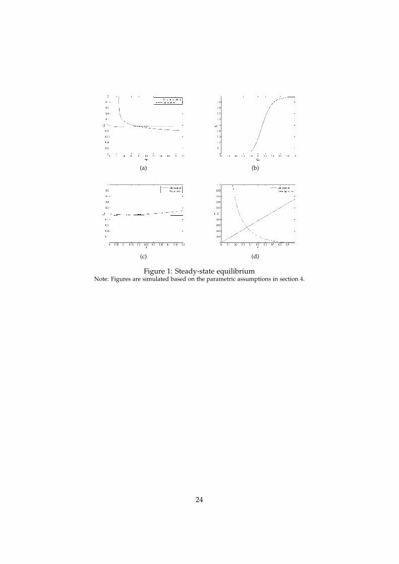
Given a certain specification of functional and parametric assumptions,the equilibrium can be solved as follows. First, combining equations (13)and (15) can eliminate the endogenous migration cut-off φ, and thus ex-press the effective wage ζm in terms of the average urban productivity z̄m.This functional link between ζm and z̄m sketches out the equilibrium ofselective migration. The solid line in figure 1(a) plots the migration con-dition. ζm is sloping downwards in terms of z̄m, suggesting the fact that ahigher urban effective wage will attract more workers to locate into cities,as plotted in panel (b), and the migrants include those with relatively lowskills, which subsequently lowers the average level of individual produc-tivity in the urban sector.

[Figure 1 about here.]

Another functional link between ζm and z̄m is from job creation in theurban labour market, obtained by merging equations (11) and (12). Asplotted with the dashed line in panel (a), the job creation condition hasan upward slope, reflecting that workers’ effective wage benefits from afavourable average level of their productivity.

The remaining equilibrium solutions for the urban labour market arestandard, as demonstrated in the last two panels of figure 1. Eliminating

10

z̄m by the migration condition, equations (11) and (12) together pin downthe equilibrium effective wage and market tightness. And the relative sizeof the urban informal sector is given by the intersection of the job creationcondition and the Beveridge curve in the vacancy-unemployment space.

4 Equilibrium analysis

Aiming to understand labour markets in developing countries, this sectioncalibrates the model to match the data for Malawi and conducts a quanti-tative analysis of the steady-state equilibrium. The calibrated model pro-vides detailed implications for urban labour informality, sectoral labourproductivity, wages and inequality.

4.1 Assumptions

Before proceeding to calibrations, some assumptions are needed. First ofall, following the quantitative analysis in Lagakos and Waugh (2013) andTemple and Ying (2014), workers’ individual productivity endowments,{za, zm}, are drawn from a continuous joint distribution. The cumulativedensity function of the distribution is given by

H (za, zm) = C [Ha (za) , Hm (zm)]

whereHa (za) = e−z−αa

a

Hm (zm) = e−z−αmm

are the marginal distributions for individual productivity in agricultureand non-agriculture respectively, given by two Fréchet distributions withsector-specific shape parameters αa and αm. A higher αa (or αm) suggestsa lower average level of productivity, and a lower skill disparity acrossindividuals within the agriculture (or non-agriculture) sector. C (u, v) is aFrank copula

C (u, v) = −1ρ

log[

1 +(e−ρu − 1) · (e−ρv − 1)

e−ρ − 1

]

11

that links two marginal distributions with a parameter of dependence,ρ ∈ (−∞, ∞) \ {0}. A positive ρ implies that workers have a positivecorrelation between their skills in agriculture and non-agriculture.

Secondly, the matching function m (u, v) is specialized to a Cobb-Douglasform with constant returns, and thus q (θ) is given by

q (θ) = µ

(1θ

)1−η

where µ is an index of matching efficiency and η denotes the elasticity ofjob matches with respect to vacancies.

4.2 Calibration

This subsection answers a key question of this paper: can the model, whenreasonably parameterized, give rise to realistic equilibrium outcomes forthe economic structure of developing countries? For this purpose, I cal-ibrate the model to match the economic structure of Malawi. Two datasets are used for the calibration: one is the Africa Sector Database (ASD,de Vries, Timmer and de Vries, 2013), and the other is the World Devel-opment Indicators (WDI). I use the ASD for the rural-urban employmentshares, and draw the unemployment rates from the WDI.

The assumptions for parameters and some equilibrium values are listedin Table 1. The employment share in the non-agriculture sector is averagedover 1991-2000. As an undeveloped country, the economy of Malawi heav-ily relies on its agricultural production. For the relative size of the urbaninformal sector, I calculate the urban unemployment rate by combiningthe urban employment share and the overall unemployment rate of thecountry averaged from 1991 to 2000, given that agriculture is assumedas a full-employment sector. The estimated size of 35 per cent is reason-able for a developing economy. It is broadly consistent with cross-countrystatistics reported by the International Labour Organisation, which implyan average of 40 per cent across 43 developing countries.10 It is also closeto the value of 30 per cent used by Satchi and Temple (2009) in their studyof Mexico, who draw on the estimate of Gong and van Soest (2002). Therecruitment cost is set at a low level as 30 per cent of the average wage in

10See laborsta.ilo.org/informal_economy_E.html for the report.

12

the formal sector, to ensure that the explanatory ability of the model doesnot rely on assuming unrealistically high recruitment costs.

Conventional values are adopted for the annual real interest rate, therate of job separation and the elasticity of job matches. The bargainingpower of workers follows Satchi and Temple (2009), who calibrate the pa-rameter based on Yashiv’s (2000) findings for Israel: firms’ asset value ofa match is low relative to average productivity. The payment to each unitof effective labour in the informal sector is fixed at 80 per cent of the for-mal sector effective wage of the baseline calibration, since the informalsector is, by the definition in Lewis (1954), comprised of low-wage occu-pations. And it also accords with cross-country evidence on the informalsector wage penalty discussed in Marcouiller et al. (1997) and Bargain andKwenda (2014), among others.

The choice of parameters for the individual productivity distributionsfollows the estimations in Temple and Ying (2014), based on micro-levelwage data from the Third Integrated Household Survey of Malawi. Thethree parameters are estimated to match the variances of log wages inagriculture and non-agriculture, and the average wage ratio across thetwo sectors simultaneously.

Finally, and without loss of generality, I set the relative price of agricul-tural goods as 0.5, and normalize the TFP in the non-agriculture sector tounity, and thus the relative TFP in agriculture is to be inferred in the base-line calibration. The matching efficiency µ is also inferred in equilibrium,as I have pinned down the steady-state matches by m = λ(1− u).

[Table 1 about here.]

The equilibrium outcomes are presented in Table 2. The first issue re-lating to the calibration is whether, under the parameter assumptions, themodel can lead to realistic equilibrium outcomes with a large rural em-ployment share and a sizable informal urban sector. The classic searchand matching framework has been a powerful tool to explain the labourmarket structure for developed countries where unemployment rates arerelatively low. However, as noted in Satchi and Temple (2009), the explana-tory power of the standard model is weakened when a large informal sec-tor exists, unless assuming an implausibly high recruitment cost, or highworker bargaining power, to eliminate the profit from opening new vacan-

13

cies. Otherwise, the standard model leads to an implausibly high vacancyrate and implies a long vacancy duration.

The calibration for this model given reasonable assumptions, on thecontrary, ends up with a standard vacancy rate of 0.05, which matchesthe observed data, even when a large number of workers are not formallyemployed, and have the agriculture sector as another option. The base-line calibration implies a vacancy duration of 23 days, which matches theevidence summarized in Satchi and Temple (2009).

[Table 2 about here.]

Meanwhile, the equilibrium reflects sectoral labour productivity in un-derdeveloped economies. Rural agriculture remains as the primary pro-duction sector, but has relatively low labour productivity. Most workers,skilled or unskilled, stay in the agriculture sector, while only those withhigh productivity are working in cities, which makes the average indi-vidual productivity in non-agriculture much higher than in agriculture.This is consistent with cross-country evidence found in Caselli (2005), anddiscussed in Gollin et al. (2014) and Lagakos and Waugh (2013).

4.3 Wages and inequality

Modelling labour heterogeneity allows for the analysis of wage distribu-tions and inequality. In the Lagakos-Waugh framework, wages and in-equality are endogenously determined, and two components contribute tothe wage distributions. First, the selective migration determines the labourcomposition in each sector, and the ‘realized’ skills of workers compose thesectoral productivity distributions. The second is the payment to each unitof effective labour, which is different across sectors but identically appliedto all workers within one sector. Based on this framework, Ying (2014)analytically derives the density functions for the wage distributions overtime, under the assumption that individual productivity endowments foragriculture and non-agriculture are not correlated, and Temple and Ying(2014) analyze the dynamics of wages and inequality during structuraltransformation when the productivity levels are correlated. In the modelof this paper, the effective wage in the urban sector is determined via Nashbargaining rather than straightforwardly given by the marginal products,

14

since the equilibrium in the urban labour market is non-Walrasian due tomatching frictions.

[Figure 2 about here.]

[Table 3 about here.]

Figure 2 plots the (log) wage distributions for each sector, along withthe overall economy, and some crucial features are summarized in Table 3.The average wage gap between agriculture and non-agriculture is mainlybecause of the difference in average individual productivity across the twosectors. As discussed in the previous section, the productivity gap is theresult of selective migration, and is commonly observed at the early stageof development.

Inequality in this paper is measured by the log variance and the Ginicoefficient. Both measures consistently show that the inequality level ofthe urban sector is higher than that of the rural sector. This finding isnot surprising, since the sectoral relative inequality level is determinedby the distribution of workers’ realized productivity in the sector, andthe distribution in the non-agriculture sector has a larger variance thanthat of the agriculture sector. It is noteworthy that in the urban sector,formally employed and self-employed workers have the same productivitydistribution, and thus the relative measure of inequality is identical forthese two groups of workers.

5 Equilibrium responses

This section evaluates some effects of varying parameters on the equilib-rium outcomes in steady state. In this model, different structural param-eters may change workers’ occupational preferences, and thus selectivemigration will take place. The reallocation of heterogeneous workers willalter labour compositions across sectors, and subsequently influence ur-ban employment, labour income and inequality.

5.1 Sectoral productivity growth

The first two experiments examine the consequences of TFP growth inthe two production sectors. Table 4 shows the outcomes of raising TFP

15

in agriculture by 20 per cent. As the rule of occupational selection sug-gests, workers with relatively low productivity in non-agriculture willleave cities for the rural sector, since their comparative advantage hasshifted to agriculture given improved rural efficiency. Therefore, the em-ployment share in the urban sector sharply declines. The urban unem-ployment rate falls in the meantime, as the agriculture sector becomes abetter option for some low-skilled workers.

Though the endowments of workers are unchanged, selective migra-tion alters the compositions of individual productivity across sectors. Theaverage productivity in non-agriculture significantly increases, as somelow skilled workers have migrated to the rural area. Workers in bothsectors will have higher average wages, but for different reasons. Theimprovement of the rural average wage is due to the increment in sec-toral efficiency, whereas the average labour income in cities rises becauseworkers’ average productivity in non-agriculture becomes higher after theselective migration takes place. The inequality level slightly declines incities, but overall inequality significantly drops, due to the expansion ofagriculture, which has less within-sector inequality.

[Table 4 about here.]

The second experiment is to raise the efficiency of the urban formalsector by 20 per cent. As shown in Table 5, it alters the comparative ad-vantage of some workers currently in agriculture, who immediately jointhe urban sector. The relative size of the informal sector sees a reduc-tion, which contradicts an implication from the Harris-Todaro model thatmigration from the rural sector will raise rather than decrease urban un-employment. But in the model of this paper, with higher non-agriculturalefficiency, workers are filling job vacancies at a faster rate, i.e. a higherθq (θ), which results in, by equation (1), a lower urban unemployment ratein steady state.

Although the effective wage in the formal sector has improved, thesectoral average wage hardly changes, because the sector is open to moreunskilled workers after the TFP growth. The inequality levels within thetwo sectors barely change, but overall inequality increases, because theurban sector, as a more unequal sector, has expanded.

[Table 5 about here.]

16

5.2 Individual productivity changes

The next two experiments evaluate how changes in the distribution of in-dividual productivity affect the steady-state equilibrium. Table 6 presentsthe equilibrium outcomes of reducing the shape parameter for agriculturalproductivity by 20 per cent. Recall that a lower shape parameter leads toa higher average level of productivity, as well as a more divergent distri-bution of skills across individuals. First of all, it is not surprising that,compared to the baseline case, the urban sector shrinks when a largernumber of workers now have comparative advantage in agriculture. Sec-ond, the relative size of the urban informal sector declines, implying anegative correlation between the urban unemployment rate and workers’average productivity in agriculture. Intuitively, it suggests that increas-ing workers’ agricultural productivity can lower urban unemployment, byreallocating individuals with relatively low non-agricultural skills to therural sector.

Average productivity and wages increase in both sectors for differ-ent reasons: in agriculture, it is directly caused by the improvement ofproductivity endowments, whereas in the urban sector, it is because thesector now has fewer but higher-skilled workers as a consequence of self-selection. The inequality levels increase, especially in the agriculture sec-tor, as the new productivity distribution in that sector has a larger disper-sion of skills.

[Table 6 about here.]

Table 7 shows the steady-state equilibrium when αm is reduced by 20per cent. By doing this, workers in the economy have a higher averagelevel in non-agricultural productivity, as well as a higher skill dispersion.The urban sector significantly expands, because the new distribution ofnon-agricultural productivity shifts some workers’ comparative advantageinto non-agriculture. Similar to the finding for agriculture, a negative re-lationship between the average individual productivity in non-agricultureand the urban unemployment rate can be observed. It further suggests,relating to policies, that the urban unemployment problem can be ame-liorated, if measures are taken to improve workers’ average productivityfor non-agriculture, even when this leads to a larger skill disparity acrossworkers.

17

The new productivity distribution doubles the average wage in cities,which increases the wage gap between agriculture and non-agriculture, orthe between-sector inequality. Meanwhile, the within-sector inequality innon-agriculture moves upwards due to the increment of the skill disper-sion. However, the inequality in agriculture slightly declines.

[Table 7 about here.]

5.3 Different labour market parameters

The last two experiments consider the consequences of changing structuralparameters in the urban labour market. Table 8 shows the equilibrium out-comes if a lower bargaining power of workers is applied. In the baselinemodel, I follow Satchi and Temple (2009) and assume workers have highbargaining power to explain the informal sector in developing countries.When the parameter of bargaining power is reduced to 0.5, a more con-ventional level, the relative size of the informal sector falls. However, inthis model, a standard parameter for workers’ bargaining power can stillcoexist with a large scale of informality, if workers are calibrated to havelower average productivity levels than the baseline model, i.e. a largerαm. In this case, the effects will be opposite to Table 7, leading to a largerinformal sector. Therefore, this model can give rise to a large informalsector even without needing to assume that workers have a high degree ofbargaining power.

[Table 8 about here.]

Table 9 shows the results of raising the parameter of matching effi-ciency, µ, by 20 per cent. With an improved efficiency, it is easier for urbanworkers and firms to build matches. As expected, the urban unemploy-ment rate falls and the effective wage increases. The non-agriculture sectorexpands slightly, as finding a formal job in cities becomes easier.

It is noteworthy that the selective migration is not sensitive to the struc-tural parameters for the urban labour market, in both of the above exper-iments. So these changes do not give rise to any significant differencesin the wage distributions within the two sectors, and barely affect the in-equality level of the economy. It suggests that policies targeted at thelabour market may not be sufficient to reduce inequality. In the calibrated

18

model of this paper, individual productivity levels are the key determi-nants of equilibrium outcomes.

[Table 9 about here.]

6 Conclusions

In this paper, I have introduced a general equilibrium model, in which het-erogeneous workers select their occupations to maximize lifetime utility,and urban workers may be unemployed due to matching frictions. Basedon the model, I investigate the interactions between selective migration,labour informality and wage inequality, and explore the effects of produc-tivity changes.

When calibrated to data, the steady-state equilibrium of the model re-flects the typical economic structure of developing countries: a consider-able agriculture sector and an informal sector in non-agriculture. A keyinnovation of the model is to show that the informal sector in developingeconomies can be explained by the distributions of labour productivity.It implies that policies to improve individual average productivity, evenwhen causing more inequality, can increase urban employment.

The wage distributions are determined by selective migration endoge-nously, where labour compositions in the two sectors play a key role. Thebaseline calibrated model shows a cross-sector wage gap, due to the differ-ence of workers’ average productivity across the two sectors. Equilibriumresponses show that changes in both sectoral and individual productivitywill have considerable effects on the labour market and wage distribu-tions. However, wages and inequality are not sensitive to changes in thestructure of the urban labour market.

For future research, the model may be extended from various perspec-tives. So far, it has been learnt that the size of the informal sector dependson individual productivity distributions, but the current model cannot tellwhether average productivity or skill dispersion has more substantial ef-fects. To evaluate their effects respectively, more parameters have to beinvolved in the distributional assumptions, which may require vast datafor calibrations. Besides, open unemployment can be modelled separatelyfrom the informal sector, so that policy implications could be studied in

19

more detail. Also, job destruction could be endogenized, which may leadto different distributions of individual productivity for the formal andinformal sectors. The dynamics out of steady-state could also be consid-ered for further implications. However, these extensions would make theanalysis more complicated, and it would have to rely more on numericalmethods.

20

References

Albrecht, J., Navarro, L. and Vroman, S. (2009). The effects of labour mar-ket policies in an economy with an informal sector, The Economic Journal119(539): pp. 1105–1129.

Amaral, P. S. and Quintin, E. (2006). A competitive model of the informalsector, Journal of Monetary Economics 53(7): pp. 1541–1553.

Bargain, O. and Kwenda, P. (2014). The informal sector wage gap: Newevidence using quantile estimations on panel data, Economic Developmentand Cultural Change 63(1): pp. 117–153.

Bosch, M. and Esteban-Pretel, J. (2012). Job creation and job destructionin the presence of informal markets, Journal of Development Economics98(2): pp. 270–286.

Burdett, K. and Mortensen, D. T. (1998). Wage differentials, employer size,and unemployment, International Economic Review 39(2): pp. 257–273.

Caselli, F. (2005). Accounting for cross-country income differences, inP. Aghion and S. N. Durlauf (eds), Handbook in Economics 22, Vol. 1, PartA of Handbook of Economic Growth, Elsevier: North-Holland, Amsterdam,pp. 679–741.

de Vries, G., Timmer, M. and de Vries, K. (2013). Structural transformationin Africa: Static gains, dynamic losses, GGDC research memorandum 136.

Gollin, D., Lagakos, D. and Waugh, M. E. (2014). The agricultural produc-tivity gap, Quarterly Journal of Economics 129(2): pp. 939–993.

Gong, X. and van Soest, A. (2002). Wage differentials and mobility in theurban labour market: a panel data analysis for Mexico, Labour Economics9(4): pp. 513–529.

Harris, J. R. and Todaro, M. P. (1970). Migration, unemployment and de-velopment: a two-sector analysis, American Economic Review 60(1): pp.126–142.

Kuralbayeva, K. and Stefanski, R. (2013). Windfalls, structural transfor-mation and specialization, Journal of International Economics 90(2): pp.273–301.

21

Lagakos, D. and Waugh, M. E. (2013). Selection, agriculture, and cross-country productivity differences, American Economic Review 103(2): pp.948–980.

Laing, D., Park, C. and Wang, P. (2005). A modified Harris-Todaro modelof rural-urban migration for China, in F. Kwan and E. Yu (eds), CriticalIssues in China’s Growth and Development, Ashgate, pp. 245 –264.

Lewis, W. A. (1954). Economic development with unlimited supplies oflabour, The Manchester School 22(2): pp. 139–191.

MacLeod, W. B. and Malcomson, J. M. (1998). Motivation and markets,American Economic Review 88(3): pp. 388–411.

Marcouiller, D., de Castilla, V. R. and Woodruff, C. (1997). Formal mea-sures of the informal-sector wage gap in Mexico, El Salvador, and Peru,Economic Development and Cultural Change 45(2): pp. 367–392.

Meghir, C., Narita, R. and Robin, J. M. (2015). Wages and informality indeveloping countries, American Economic Review. Forthcoming.

Merz, M. (1995). Search in the labor market and the real business cycle,Journal of Monetary Economics 36(2): pp. 269–300.

Moene, K. O. (1988). A reformulation of the Harris-Todaro mechanismwith endogenous wages, Economics Letters 27(4): pp. 387–390.

Mortensen, D. T. and Pissarides, C. A. (1994). Job creation and job destruc-tion in the theory of unemployment, Review of Economic Studies 61(3): pp.397–415.

Mortensen, D. T. and Pissarides, C. A. (1999). New developments in mod-els of search in the labor market, Vol. 3, Part B of Handbook of LaborEconomics, Elsevier, pp. 2567–2627.

Pissarides, C. (2000). Equilibrium Unemployment Theory, MIT, Mas-sachusetts.

Pries, M. J. (2008). Worker heterogeneity and labor market volatility inmatching models, Review of Economic Dynamics 11(3): pp. 664–678.

22

Roy, A. D. (1951). Some thoughts on the distribution of earnings, OxfordEconomic Papers 3(2): pp. 135–146.

Satchi, M. and Temple, J. (2009). Labor markets and productivity in devel-oping countries, Review of Economic Dynamics 12(1): pp. 183–204.

Sato, Y. (2004). Migration, frictional unemployment, and welfare-improving labor policies, Journal of Regional Science 44(4): pp. 773–793.

Strand, J. (1987). Unemployment as a discipline device with heterogeneouslabor, American Economic Review 77(3): pp. 489–493.

Temple, J. and Ying, H. (2014). Life during structural transformation, Dis-cussion paper 10297, CEPR.

Todaro, M. P. (1969). A model of labor migration and urban unemploy-ment in less developed countries, American Economic Review 59(1): pp.138–148.

Yashiv, E. (2000). The determinants of equilibrium unemployment, Ameri-can Economic Review 90(5): pp. 1297–1322.

Ying, H. (2014). Growth and structural change in a dynamic Lagakos-Waugh model, Working paper 14/639, University of Bristol.

Young, A. (2013). Inequality, the urban-rural gap, and migration, QuarterlyJournal of Economics 128(4): pp. 1727–1785.

Zenou, Y. (2008). Job search and mobility in developing countries. theoryand policy implications, Journal of Development Economics 86(2): pp. 336–355.

Zenou, Y. (2011). Rural–urban migration and unemployment: Theory andpolicy implications, Journal of Regional Science 51(1): pp. 65–82.

23

(a) (b)

(c) (d)

Figure 1: Steady-state equilibriumNote: Figures are simulated based on the parametric assumptions in section 4.

24

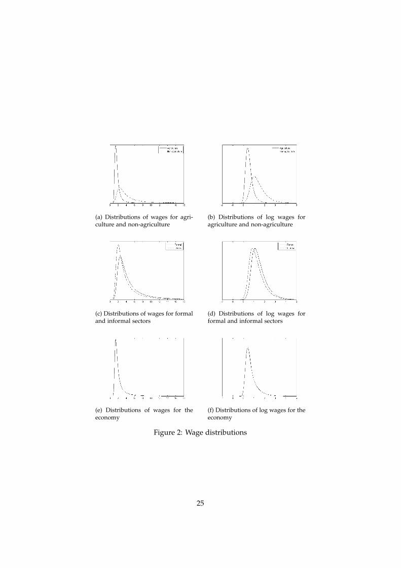
(a) Distributions of wages for agri-culture and non-agriculture

(b) Distributions of log wages foragriculture and non-agriculture

(c) Distributions of wages for formaland informal sectors

(d) Distributions of log wages forformal and informal sectors

(e) Distributions of wages for theeconomy

(f) Distributions of log wages for theeconomy

Figure 2: Wage distributions

25

Table 1: Parameter and other baseline assumptions

Parameters/assumptions ValueUrban employment share (Lm) 0.21Informal sector share of urban labour (u) 0.35Recruitment cost/Average formal sector wage 0.30

Interest rate (r) 0.04Job separation rate (λ) 0.06Elasticity of job matches (η) 0.50Bargaining power for workers (β) 0.70Informal-formal effective wage ratio 0.80

Productivity distribution in agriculture (αa) 3.40Productivity distribution in non-agriculture (αm) 1.53Productivity dependence (ρ) 6.93

Table 2: Equilibrium outcomes

Urban employment share (Lm) 0.21Informal sector share of urban labour (u) 0.35

Vacancy rate (v) 0.05Matching rate (m) 0.04Vacancy duration (days) 23Effective wage in formal sector (ζm) 0.96

Average productivity in agriculture (z̄a) 1.22Average productivity in non-agriculture (z̄m) 7.58. Rural-urban ratio 0.16

26

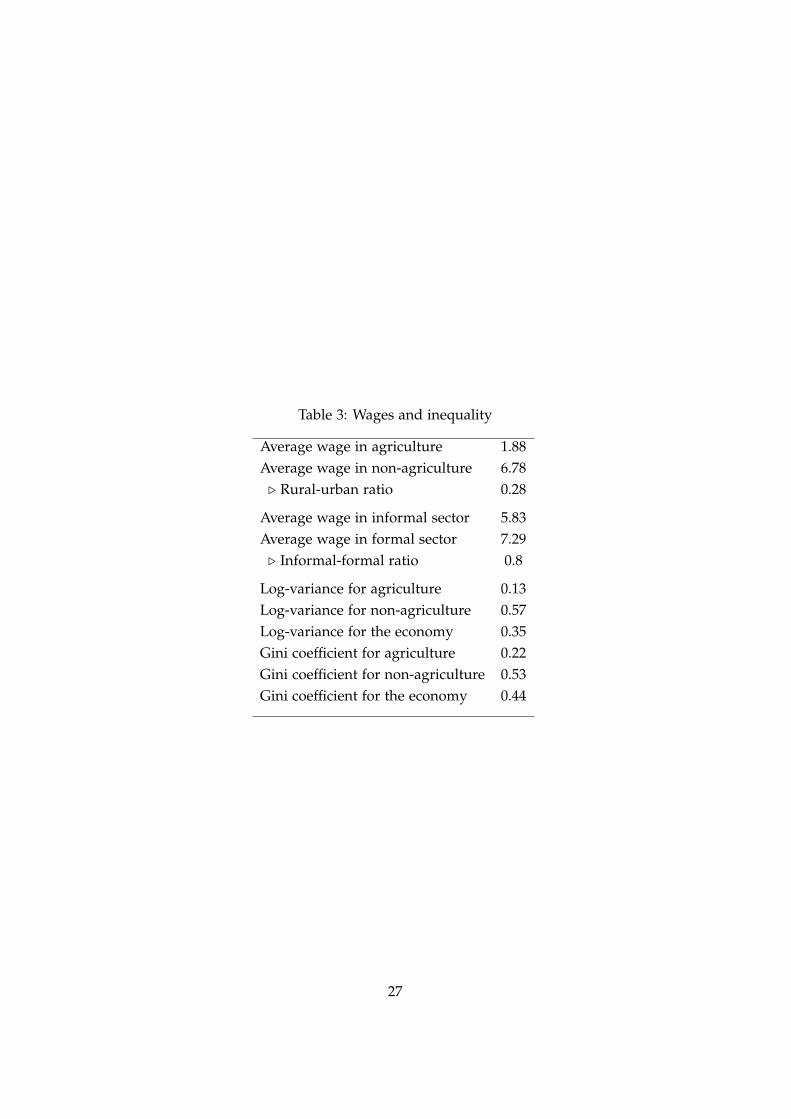
Table 3: Wages and inequality

Average wage in agriculture 1.88Average wage in non-agriculture 6.78. Rural-urban ratio 0.28

Average wage in informal sector 5.83Average wage in formal sector 7.29. Informal-formal ratio 0.8

Log-variance for agriculture 0.13Log-variance for non-agriculture 0.57Log-variance for the economy 0.35Gini coefficient for agriculture 0.22Gini coefficient for non-agriculture 0.53Gini coefficient for the economy 0.44

27

Table 4: Effects of raising TFP in agriculture by 20%

Baseline New Change (+%)Urban employment share 0.21 0.15 −28.6Informal sector share of urban labour 0.35 0.32 −8.57Vacancy rate 0.05 0.06 20.0Matching rate 0.04 0.04 0Effective wage in formal sector 0.96 0.96 0

Average productivity in agriculture 1.22 1.23 0.82Average productivity in non-agriculture 7.58 9.39 23.9. Rural-urban ratio 0.16 0.13 −18.8

Average wage in agriculture 1.88 2.29 21.8Average wage in non-agriculture 6.78 8.47 24.9. Rural-urban ratio 0.28 0.27 −3.57

Average wage in informal sector 5.83 7.22 23.8Average wage in formal sector 7.29 9.05 24.1. Informal-formal ratio 0.80 0.80 0

Log-variance for agriculture 0.13 0.13 0Log-variance for non-agriculture 0.57 0.56 −1.75Log-variance for the economy 0.35 0.30 −14.3Gini coefficient for agriculture 0.22 0.22 0Gini coefficient for non-agriculture 0.53 0.52 −1.89Gini coefficient for the economy 0.44 0.40 −9.09

28

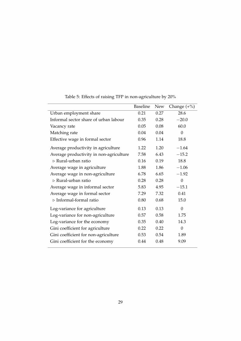
Table 5: Effects of raising TFP in non-agriculture by 20%

Baseline New Change (+%)Urban employment share 0.21 0.27 28.6Informal sector share of urban labour 0.35 0.28 −20.0Vacancy rate 0.05 0.08 60.0Matching rate 0.04 0.04 0Effective wage in formal sector 0.96 1.14 18.8

Average productivity in agriculture 1.22 1.20 −1.64Average productivity in non-agriculture 7.58 6.43 −15.2. Rural-urban ratio 0.16 0.19 18.8

Average wage in agriculture 1.88 1.86 −1.06Average wage in non-agriculture 6.78 6.65 −1.92. Rural-urban ratio 0.28 0.28 0

Average wage in informal sector 5.83 4.95 −15.1Average wage in formal sector 7.29 7.32 0.41. Informal-formal ratio 0.80 0.68 15.0

Log-variance for agriculture 0.13 0.13 0Log-variance for non-agriculture 0.57 0.58 1.75Log-variance for the economy 0.35 0.40 14.3Gini coefficient for agriculture 0.22 0.22 0Gini coefficient for non-agriculture 0.53 0.54 1.89Gini coefficient for the economy 0.44 0.48 9.09

29

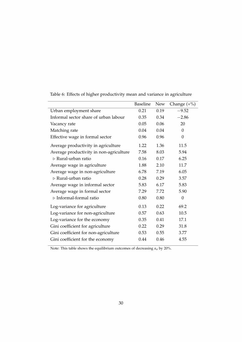
Table 6: Effects of higher productivity mean and variance in agriculture

Baseline New Change (+%)Urban employment share 0.21 0.19 −9.52Informal sector share of urban labour 0.35 0.34 −2.86Vacancy rate 0.05 0.06 20Matching rate 0.04 0.04 0Effective wage in formal sector 0.96 0.96 0

Average productivity in agriculture 1.22 1.36 11.5Average productivity in non-agriculture 7.58 8.03 5.94. Rural-urban ratio 0.16 0.17 6.25

Average wage in agriculture 1.88 2.10 11.7Average wage in non-agriculture 6.78 7.19 6.05. Rural-urban ratio 0.28 0.29 3.57

Average wage in informal sector 5.83 6.17 5.83Average wage in formal sector 7.29 7.72 5.90. Informal-formal ratio 0.80 0.80 0

Log-variance for agriculture 0.13 0.22 69.2Log-variance for non-agriculture 0.57 0.63 10.5Log-variance for the economy 0.35 0.41 17.1Gini coefficient for agriculture 0.22 0.29 31.8Gini coefficient for non-agriculture 0.53 0.55 3.77Gini coefficient for the economy 0.44 0.46 4.55

Note: This table shows the equilibrium outcomes of decreasing αa by 20%.

30

Table 7: Effects of higher productivity mean and variance in non-agriculture

Baseline New Change (+%)Urban employment share 0.21 0.30 42.9Informal sector share of urban labour 0.35 0.26 −25.7Vacancy rate 0.05 0.09 80.0Matching rate 0.04 0.04 0Effective wage in formal sector 0.96 0.97 1.04

Average productivity in agriculture 1.22 1.17 −4.10Average productivity in non-agriculture 7.58 14.4 90.0. Rural-urban ratio 0.16 0.08 −100

Average wage in agriculture 1.88 1.81 −3.72Average wage in non-agriculture 6.78 13.1 93.2. Rural-urban ratio 0.28 0.14 −100

Average wage in informal sector 5.83 11.0 88.7Average wage in formal sector 7.29 13.8 89.3. Informal-formal ratio 0.80 0.79 −1.25

Log-variance for agriculture 0.13 0.12 −7.69Log-variance for non-agriculture 0.57 0.83 45.6Log-variance for the economy 0.35 0.57 62.9Gini coefficient for agriculture 0.22 0.21 −4.55Gini coefficient for non-agriculture 0.53 0.73 37.7Gini coefficient for the economy 0.44 0.66 50.0

Note: This table shows the equilibrium outcomes of decreasing αm by 20%.

31

Table 8: Effects of lower bargaining power

Baseline New Change (+%)Urban employment share 0.21 0.21 0Informal sector share of urban labour 0.35 0.26 −25.7Vacancy rate 0.05 0.09 80.0Matching rate 0.04 0.04 0Effective wage in formal sector 0.96 0.94 −2.08

Average productivity in agriculture 1.22 1.21 −0.82Average productivity in non-agriculture 7.58 7.51 −0.92. Rural-urban ratio 0.16 0.16 0

Average wage in agriculture 1.88 1.88 0Average wage in non-agriculture 6.78 6.72 −0.88. Rural-urban ratio 0.28 0.28 0

Average wage in informal sector 5.83 5.78 −0.86Average wage in formal sector 7.29 7.05 −3.29. Informal-formal ratio 0.80 0.82 25.0

Log-variance for agriculture 0.13 0.13 0Log-variance for non-agriculture 0.57 0.57 0Log-variance for the economy 0.35 0.35 0Gini coefficient for agriculture 0.22 0.22 0Gini coefficient for non-agriculture 0.53 0.53 0Gini coefficient for the economy 0.44 0.44 0

Note: This table shows the outcomes of using a common value of β, 0.5, rather than 0.7.

32

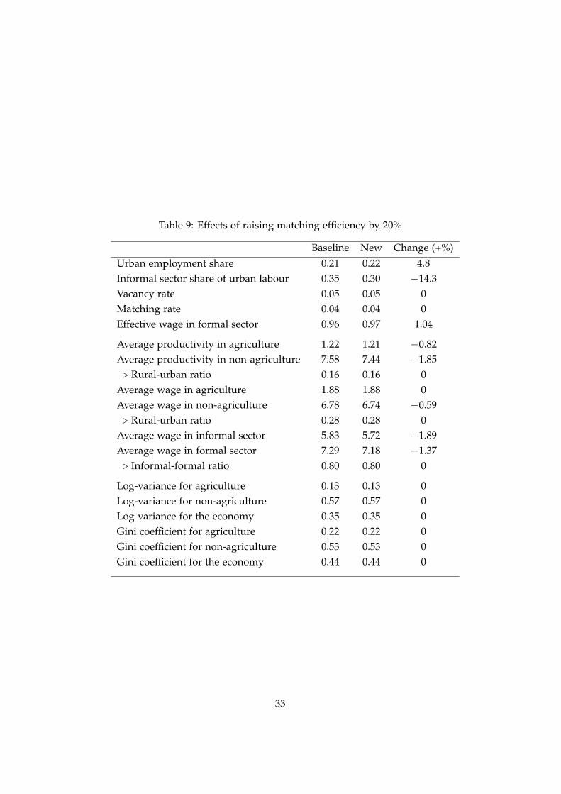
Table 9: Effects of raising matching efficiency by 20%

Baseline New Change (+%)Urban employment share 0.21 0.22 4.8Informal sector share of urban labour 0.35 0.30 −14.3Vacancy rate 0.05 0.05 0Matching rate 0.04 0.04 0Effective wage in formal sector 0.96 0.97 1.04

Average productivity in agriculture 1.22 1.21 −0.82Average productivity in non-agriculture 7.58 7.44 −1.85. Rural-urban ratio 0.16 0.16 0

Average wage in agriculture 1.88 1.88 0Average wage in non-agriculture 6.78 6.74 −0.59. Rural-urban ratio 0.28 0.28 0

Average wage in informal sector 5.83 5.72 −1.89Average wage in formal sector 7.29 7.18 −1.37. Informal-formal ratio 0.80 0.80 0

Log-variance for agriculture 0.13 0.13 0Log-variance for non-agriculture 0.57 0.57 0Log-variance for the economy 0.35 0.35 0Gini coefficient for agriculture 0.22 0.22 0Gini coefficient for non-agriculture 0.53 0.53 0Gini coefficient for the economy 0.44 0.44 0

33