W Wiilldd FFiisshheerriieess · Simon D. Goldsworthy, Brad Page, Paul Rogers and Tim Ward SARDI...
175
W W W i i i l l l d d d F F F i i i s s s h h h e e e r r r i i i e e e s s s Establishing ecosystem-based management for the South Australian Sardine Fishery: developing ecological performance indicators and reference points to assess the need for ecological allocations Final Report to the Fisheries Research and Development Corporation Simon D. Goldsworthy, Brad Page, Paul Rogers and Tim Ward SARDI Publication No. F2010/000863-1 SARDI Research Report Series No. 529 ISBN: 978-1-921563-38-6 FRDC PROJECT NO. 2005/031 SARDI Aquatic Sciences PO Box 120 Henley Beach SA 5022 March 2011
Transcript of W Wiilldd FFiisshheerriieess · Simon D. Goldsworthy, Brad Page, Paul Rogers and Tim Ward SARDI...

WWWiiilllddd FFFiiissshhheeerrriiieeesss
Establishing ecosystem-based management for the South Australian Sardine Fishery: developing ecological performance indicators and reference
points to assess the need for ecological allocations
Final Report to the Fisheries Research and Development Corporation
Simon D. Goldsworthy, Brad Page, Paul Rogers and Tim Ward
SARDI Publication No. F2010/000863-1 SARDI Research Report Series No. 529
ISBN: 978-1-921563-38-6
FRDC PROJECT NO. 2005/031
SARDI Aquatic Sciences PO Box 120 Henley Beach SA 5022
March 2011

Establishing ecosystem-based management for the
South Australian Sardine Fishery: developing ecological performance indicators and reference
points to assess the need for ecological allocations
Final Report to the Fisheries Research and Development Corporation
Simon D. Goldsworthy, Brad Page, Paul Rogers
and Tim Ward
SARDI Publication No. F2010/000863-1 SARDI Research Report Series No. 529
ISBN: 978-1-921563-38-6
FRDC PROJECT NO. 2005/031
March 2011

This publication may be cited as: Goldsworthy, S.D., Page, B., Rogers, P. and Ward, T (2011). Establishing ecosystem-based management for the South Australian Sardine Fishery: developing ecological performance indicators and reference points to assess the need for ecological allocations. Final Report to the Fisheries Research and Development Corporation. South Australian Research and Development Institute (Aquatic Sciences), Adelaide. SARDI Publication No. F2010/000863-1. SARDI Research Report Series No. 529. 173pp. South Australian Research and Development Institute SARDI Aquatic Sciences 2 Hamra Avenue West Beach SA 5024 Telephone: (08) 8207 5400 Facsimile: (08) 8207 5406 http://www.sardi.sa.gov.au
DISCLAIMER
The authors do not warrant that the information in this document is free from errors or omissions. The authors do not accept any form of liability, be it contractual, tortuous, or otherwise, for the contents of this document or for any consequences arising from its use or any reliance placed upon it. The information, opinions and advice contained in this document may not relate, or be relevant, to a readers particular circumstances. Opinions expressed by the authors are the individual opinions expressed by those persons and are not necessarily those of the publisher, research provider or the Fisheries Research and Development Institute. The Fisheries Research and Development Corporation plans, invests in and manages fisheries research and development throughout Australia. It is a statutory authority within the portfolio of the federal Minister for Agriculture, Fisheries and Forestry, jointly funded by the Australian Government and the fishing industry.
© 2011 SARDI & FRDC
This work is copyright. Except as permitted under the Copyright Act 1968 (Cth), no part may be reproduced by any process, electronic or otherwise, without the specific written permission of the copyright owners. Information may not be stored electronically in any form whatsoever without such permission. Printed in Adelaide: March 2011 SARDI Publication No. F2010/000863-1 SARDI Research Report Series No. 529 ISBN: 978-1-921563-38-6 FRDC PROJECT NO. 2005/031 Author(s): Simon D. Goldsworthy, Brad Page, Paul Rogers and Tim Ward Reviewer(s): Alex Ivey, Cameron Dixon, Shane Roberts, David Currie, Maylene Loo, Adrian
Linnane and Anthony Fowler. Approved by: Dr Jason Tanner
Principal Scientist - Marine Environment & Ecology
Signed: Date: 24 March 2011 Distribution: Fisheries Research and Development Corporation, SAASC Library, University of
Adelaide Library, Parliamentary Library, State Library and National Library
Circulation: Public Domain

Contents 2
TABLE OF CONTENTS 1 NON TECHNICAL SUMMARY ....................................................................................... 9
2 BACKGROUND: ASSESSING THE NEED FOR ECOLOGICAL ALLOCATIONS IN AUSTRALIA’S LARGEST SMALL PELAGIC FISHERY.............................................. 15
ECOSYSTEM-BASED FISHERIES MANAGEMENT (EBFM) ......................................................... 15 Global, regional and national treaties and legislation supporting adoption of EBFM in Australia ........................................................................................................................ 16 Ecological allocation and spatial limitation .................................................................... 17 Oceanography and Ecology of the Great Australian Bight............................................ 19
THE SOUTH AUSTRALIAN SARDINE FISHERY (SASF) ............................................................. 20 Overview ....................................................................................................................... 20 Management of the SASF............................................................................................. 23 Need for EBFM in the SASF ......................................................................................... 25
OBJECTIVES ......................................................................................................................... 26 THE APPROACH .................................................................................................................... 26 NEED ................................................................................................................................... 29
3 THE DIETS OF THE MARINE PREDATORS IN SOUTHERN AUSTRALIA: ASSESSING THE NEED FOR ECOSYSTEM-BASED MANAGEMENT OF THE SOUTH AUSTRALIAN SARDINE FISHERY ................................................................ 31
INTRODUCTION ..................................................................................................................... 31 Pelagic fishes and sharks ............................................................................................. 32 Squids ........................................................................................................................... 32 Seabirds ........................................................................................................................ 33 Marine mammals........................................................................................................... 33 SA Sardine Fishery (SASF) .......................................................................................... 34
MATERIALS AND METHODS .................................................................................................... 34 RESULTS.............................................................................................................................. 36
Guilds based on diet of predator groups ....................................................................... 51 DISCUSSION ......................................................................................................................... 56
4 SPATIAL DISTRIBUTION OF CONSUMPTION EFFORT OF KEY APEX PREDATORS AND THEIR OVERLAP WITH THE SA SARDINE FISHERY....................................... 61
INTRODUCTION ..................................................................................................................... 61 MATERIALS AND METHODS .................................................................................................... 62
Satellite telemetry data.................................................................................................. 62 Filtering and analysis of time spent in areas ................................................................. 62 Model development....................................................................................................... 63
RESULTS.............................................................................................................................. 64 DISCUSSION ......................................................................................................................... 66

Contents 3
5 TROPHODYNAMICS OF THE EASTERN GREAT AUSTRALIAN BIGHT PELAGIC ECOSYSTEM: IMPLICATIONS FOR ASSESSING THE ECOLOGICAL SUSTAINABILITY OF AUSTRALIA’S LARGEST FISHERY ....................................... 77
INTRODUCTION ..................................................................................................................... 77 MATERIALS AND METHODS .................................................................................................... 81
Ecopath and mass balance approach........................................................................... 81 Model area and structure .............................................................................................. 81 Model fitting................................................................................................................... 83 Ecosystem indicators .................................................................................................... 84 Model scenarios ............................................................................................................ 84
RESULTS.............................................................................................................................. 85 Trophic structure and flow............................................................................................. 85 Time-series fitting.......................................................................................................... 86 Temporal changes in group biomass ............................................................................ 87 Ecosystem indicators .................................................................................................... 88 Model scenario results .................................................................................................. 89
DISCUSSION ......................................................................................................................... 91
6 IDENTIFICATION OF ECOLOGICAL PERFORMANCE INDICATORS FOR NATURAL PREDATORS OF SARDINE SARDINOPS SAGAX IN SOUTHERN AUSTRALIA: ASSESSING THE NEED FOR ECOSYSTEM-BASED MANAGEMENT OF THE SOUTH AUSTRALIAN SARDINE FISHERY .............................................................. 116
INTRODUCTION ................................................................................................................... 116 MATERIALS AND METHODS ................................................................................................. 119 RESULTS............................................................................................................................ 122 DISCUSSION ....................................................................................................................... 127
7 BENEFITS AND ADOPTION ...................................................................................... 133
INDUSTRY/COMMUNITY SECTORS BENEFITING FROM RESEARCH ........................................... 133 ADOPTION OF THE RESEARCH BY IDENTIFIED BENEFICIARIES ................................................ 135 SUMMARY OF PROJECT EXTENSION TO BENEFICIARIES ......................................................... 135 HOW BENEFITS AND BENEFICIARIES COMPARE TO THOSE IDENTIFIED IN THE ORIGINAL
APPLICATION ...................................................................................................................... 135
8 FURTHER DEVELOPMENT ....................................................................................... 136
9 PLANNED OUTCOMES.............................................................................................. 137
SOCIAL, ECONOMIC AND ECOLOGICAL ADVANTAGES............................................................. 137 ECOLOGICALLY SUSTAINABLE MANAGEMENT OF THE SA SARDINE FISHERY ........................... 137 CONSERVATION OF SEABIRD AND MARINE MAMMAL POPULATIONS ........................................ 137
10 CONCLUSIONS .......................................................................................................... 138
11 REFERENCES ............................................................................................................ 141

Contents 4
12 APPENDICES ............................................................................................................. 156
APPENDIX 1: STAFF ............................................................................................................ 156 APPENDIX 2: INTELLECTUAL PROPERTY AND VALUABLE INFORMATION................................... 156 APPENDIX 3: FUNCTIONAL GROUPS (BY COMMON NAMES) DEVELOPED IN THE EGAB MODEL. 157 APPENDIX 4: SUMMARY OF THE BIOLOGY OF THE FUNCTIONAL GROUPS USED IN THE EGAB
MODEL ............................................................................................................................... 159 Appendix 4.1 Baleen whales (model group 1) ............................................................ 159 Appendix 4.2 Toothed whales/dolphins (model groups 2 &3) ..................................... 160 Appendix 4.3 Seals (model groups 4-6) ...................................................................... 161 Appendix 4.4 Seabirds (model groups 7-10)............................................................... 163 Appendix 4.5 Pelagic sharks (model group 11) .......................................................... 166 Appendix 4.6 Demersal sharks (model group 12)....................................................... 167 Appendix 4.7 Rays and Skates (model group 13)....................................................... 168 Appendix 4.8 Southern Bluefin Tuna (SBT) (model group 14).................................... 168 Appendix 4.9 Other tunas and kingfish (model group 15) ........................................... 169 Appendix 4.10 Large bentho-pelagic piscivorous fish (model group 16) .................... 169 Appendix 4.11 Small pelagic fish (groups 17-22)........................................................ 169 Appendix 4.12 Australian Salmon and Australian herring (model group 23)............... 170 Appendix 4.13 Small to medium demersal fishes (model groups. 24–27, 29) ............ 171 Appendix 4.14 Mesopelagics (model group 28).......................................................... 171 Appendix 4.15 Cephalopods (model group 30–33)..................................................... 172 Appendix 4.16 Zooplankton (model groups 34–35) .................................................... 172 Appendix 4.17 Benthic grazers (megabenthos) (model group 36).............................. 172 Appendix 4.18 Detritivores (infauna-macrobenthos) (model group 37)....................... 173 Appendix 4.19 Filter feeders (model group 38)........................................................... 173 Appendix 4.20 Primary Producers (model group 39) .................................................. 173 Appendix 4.21 Detritus (model group 40) ................................................................... 173

Contents 5
LIST OF FIGURES Figure 2.1. (a) Total catches of sardine from logbook records, catch disposal records (CDR) and estimated lost catches, (b) fishing effort (boat-days and net sets), and (c) mean annual catch per unit effort (tonnes per boat-days and net sets +/- SE) (Ward et al. 2010). ............21
Figure 2.2. Spatial trends in annual catches of sardine between 2001 and 2009 (Ward et al. 2010)...................................................................................................................................................22
Figure 2.3. TACC for the SA sardine fishery between 1991-2009 (hatched TACC for 2010 is to be caught outside the traditional fishing area) (Ward et al. 2010)........................................24
Figure 2.4. Daily Egg Production Method estimates of sardine spawning biomass in South Australian waters from 1995-2009. Error bars are 95% confidence intervals (Ward et al. 2010)...................................................................................................................................................24
Figure 3.1. Bray-Curtis similarity dendrogram of the diets of the 37 predator groups. Significantly different guilds are numbered 1-8 at the bottom of the dendrogram (abbreviations: LT: long trip, ST: short trip, JUV: juvenile, AF: adult female, AM: adult male)..............................................................................................................................................................52
Figure 4.1. Estimated spatial distribution of foraging and consumption (t/y) effort by five key land-breeding apex predators: A NZFS, B ASL, C little penguins, D STSW, E crested tern and F all species combined. Foraging and consumption by species outside of shelf waters has been excluded. Data for crested terns and little penguins are restricted to the chick rearing period (4 and 9 months, respectively). For all other species, plots represent total annual consumption. Data for ASL are from Goldsworthy et al. (2010). .................................68
Figure 4.2. Estimated spatial distribution of consumption of fish (A), cephalopods (B), crustaceans (C) and sardines (D) (t/y) by the five key land-breeding apex predators combined; spatial distribution of the mean annual catch of sardines (1999-2010) by the SA sardine fishery (E) and a plot demonstrating the overlap in fishery catch and apex predator consumption of sardines (F). ..........................................................................................................69
Figure 5.1. Location of the eastern Great Australian Bight (EGAB) ecosystem included in the Ecopath with Ecosim model. The depth contours are 100, 200, 500, 1000 and 2000m............................................................................................................................................................102
Figure 5.2. Trends in the total landings (catch t y-1) from eight main fisheries in the EGAB ecosystem between 1991 and 2008. The inset graph excludes sardine landings so that trends in the remaining fleets can be more easily resolved.....................................................103
Figure 5.3. Food web diagram of the Ecopath model of the EGAB ecosystem. Functional groups are indicated by circles, with size proportional to their biomass. The trophic links between groups are indicated by lines........................................................................................104
Figure 5.4. Mixed trophic impacts based on the Ecopath model of the EGAB ecosystem. It shows the direct and indirect impact that small increase in the biomass of groups listed in rows (Impacting group) have on those listed in columns (Impacted group). Filled circles indicated positive impacts, open circles negative. The size of the circle represents the relative scale of the impact............................................................................................................105
Figure 5.5. Estimated proportional breakdown of total annual conumption of sardines and of all small pelagic fish (sardine, anchovey, blue mackerel, jack mackerel, redbait and inshore planktivores) by their predators based on the Ecopath model of the EGAB ecosystem. Total consumption of sardines and of all small pelagic fishes is estimed to be 123,369 t y-1 and 396,129 t y-1, respectively. ............................................................................................................106

Contents 6
Figure 5.6. Mean monthly windstress values between 1991 and 2008 (scaled to the value for January 1991, grey dotted line), plotted against the Ecosim modelled windstress anomoly, with overal trend (dashed black line) and values of the slope and coefficient of variation (r2). ....................................................................................................................................107
Figure 5.7. Time series fits of the EGAB Ecosim model (thin line) to observed biomass (CPUE) and catch data (dots) for 16 functional groups between 1991 and 2008. The modelled trend lines (dashed) are provided, together with values of the slope and coefficient of variation (r2) (see overleaf for remaining plots). .................................................108
Figure 5.8. Estimated changes in the biomass of high trophic level predators based on the Ecosim EGAB model between 1991 and 2008: A) marine mammals and birds; b) sharks, rays and skates, tunas and kingfish. Biomass change in NZ and Australian fur seals is forced in the model as these estimates are based on empircal data for these species in the EGAB ecosystem. ..........................................................................................................................110
Figure 5.9. Estimated changes in the biomass of small pelagic fish functional groups, arrow squid and calarmary based on the Ecosim EGAB model between 1991 and 2008. ...........111
Figure 5.10. Ecosystem indicators calculated from the Ecosim EGAB model for the period 1991 to 2008. A. Changes in the landings (catch t y-1) of all fleets (total catch), sardine catch and other catch; B. Kempton’s Q biomass diversity index; C. Mean trophic level of the catch and D. Fishing In Balance (FIB) index. Estimated trends are given by dashed lines (regression), with their coefficient of variation (r2) and level of significance (P). ..................112
Figure 5.11. Predicted change in the biomass of functional groups in the Ecosim EGAB model in 2040 relative to 2008 with sardine biomass reduced to 0.75, 0.50 and 0.25 of 2008 biomass. In this simulation, NZ fur seal and Australian fur seal groups were forced to increase between 2008 and 2040 (in line with observed increases between 1991 and 2008), so that population abundances in the EGAB were about 1.5 and 7.0 times present (2008) levels, respectively (with no change in sardine biomass). Note: the break in the scale of the x-axis. ....................................................................................................................................113
Figure 5.12. Predicted change in the biomass of functional groups in the Ecosim EGAB model in 2040 relative to 2008 with biomass increases of SBT. Biomass increases in SBT were simulated by reducing effort in the purse seine fishery by adjusting time series values between 2008 and 2040 under different scenarios of fishing effort (current [2008] levels; 50% 2008 levels; 25% 2008 levels and no fishing effort). In these simulations, NZ fur seal and Australian fur seal groups were forced to increase between 2008 and 2040 (in line with observed increases between 1991 and 2008), so that populations abundances in the EGAB were about 1.5 and 7.0 times present (2008), respectively. ....................................................114
Figure 5.13. Predicted change in the biomass of functional groups in the Ecosim EGAB model in 2040 relative to 2008 with different scenarios of arrow squid biomass reduction and with no SBT fishery. Biomass redcution in arrow squid were simulated by adjusting time series values between 2008 and 2040 under different scenarios of fishing effort (current [2008] levels; 50% biomass reduction of 2008 levels; 75% biomass reduction of 2008 levels). In these simulations, NZ fur seal and Australian fur seal groups were forced to increase between 2008 and 2040 (in line with observed increases between 1991 and 2008), so that populations abundances in the EGAB were about 1.5 and 7.0 times present (2008), respectively. .......................................................................................................................115

Contents 7
LIST OF TABLES Table 3.1. Predator group and sample sizes compiled in this study. The source of the data and method used to summarise the data (based on biomass estimation or numerical abundance) are indicated. Data are grouped by guild (see Figure 3.1) and within guild into alphabetical order. ............................................................................................................................38
Table 3.2. Percent contribution of prey taxa to the diet of each predator. Guilds of predators and habitats of prey taxa (benthic (B), pelagic (P) or terrestrial (T) in the prey taxa column) are also indicated. ............................................................................................................................39
Table 3.3. SIMPER results for prey taxa that contributed to the differences between guilds (reported as SIMPER percentage). Only prey taxa that were consumed by a guild are reported for that guild (prey taxa that were not consumed by a guild can contribute to differences between guilds if the other guild used the taxa)......................................................53
Table 3.4. Habitat classification of each predator group, based on the habitat of the majority of their prey and sorted by guilds. ..................................................................................................55
Table 4.1. Location of breeding colonies of five land-breeding apex predators in the EGAB ecosystem, and the estimated percentage contribution that each colony represents relative to the total EGAB population of that species................................................................................70
Table 4.2. Details on the numbers of individual apex predators instrumented with satellite transmitters and/or GPS tags, and the number of foraging trips recorded. The best model fit (normal or gamma distribution) for depth and distance parameters for each taxa group are provided. The maximum depth and distance from colony, and the mean and standard deviation (SD) and the shape and slope parameters of pooled depth and distance distributions for each taxa group based on the pertinent function are also presented. Details of the model used for ASL are presented in Goldsworthy et al. (2010). ..................................75
Table 4.3. Estimated total annual consumption and the total annual consumption in the EGAB ecosystem, including a breakdown of prey into the following categories: small pelagic fish, sardines, all fish, cephalopods and crustaceans. All estimates in t/y are derived from diet, population biomass and consumption estimates from Chapter 5. ..........................76
Table 5.1. Functional groups and their diet matrix showing proportional prey contribution used in the balanced EGAB Ecopath model. ...............................................................................96
Table 5.2. Summary of fleet landings (catch t km-2) by functional group used in the balanced EGAB Ecopath model. .....................................................................................................................98
Table 5.3. Summary of fleet discards (catch t km-2) by functional group used in the balanced EGAB Ecopath model. .....................................................................................................................99
Table 5.4. Biological parameters by functional group of the balanced EGAB Ecopath model. Parameters in bold were estimated by the model. P/B = production/biomass; Q/B = consumption/biomass; EE = ecotrophic efficiency. ...................................................................100
Table 5.5. Change of estimated relative biomass of key taxa groups based on Ecosim simulations of the EGAB ecosystem between 1991 and 2008, without and with primary production (PP) forcing; and between 2008 and 2040 with no PP forcing, with SBT fishery catch removed and with a 50% reduction in arrow squid biomass. ........................................101
Table 6.1. The number of EPIs that were significant for each correlation. EPIs that describe similar relationships are grouped, but each relationship is for a different test, based on different data sets (e.g. the EPI for crested terns anchovy proportion in diet summarises the

Contents 8
relationship between the diet of crested terns, at several different times of the year versus the fishery parameters)..................................................................................................................124
Table 6.2. Correlation coefficient for significant correlations (maximum coefficient for negative correlations and minimum for positive correlations). EPI that describe similar relationships are grouped, but each relationship is for a different test, based on different data sets (e.g. the EPI for crested terns anchovy proportion in diet summarises the relationship between the diet of crested terns, at several different times of the year versus the fishery parameters)..................................................................................................................126
Table 6.3. Potential EPI to implement EBFM in the SA sardine fishery. The EPIs are based on the breeding and feeding ecology of E. minor, P. tenuirostris, S. bergii and A. forsteri, and were found to be either negatively related to the fishery catch of S. sagax or positively related to the spawning biomass of S. sagax. Estimates of the number of days required to collect the data are provided.........................................................................................................127

Non Technical Summary 9
1 NON TECHNICAL SUMMARY
2005/031 Establishing ecosystem-based management for the South Australian Sardine Fishery: developing ecological performance indicators and reference points to assess the need for ecological allocations
PRINCIPAL INVESTIGATOR: Dr Tim Ward ADDRESS: South Australian Research and Development Institute (SARDI) Aquatic Sciences, PO Box 120, Henley Beach SA 5022, Telephone: 08 8207 5400 Fax: 08 8207 5481 OBJECTIVES 1. To identify species of key marine predators that consume significant quantities of sardine and could potentially be used to assess the need for ecological and/or spatial allocations in the SA Sardine Fishery. 2. To identify population parameters for these key marine predators, such as measures of foraging and/or reproductive success, that are likely to be affected by changes in the distribution and abundance of sardine, and which could potentially act as ecological performance indicators for the fishery. 3. To examine the spatial and temporal scales at which these performance indicators vary in order to develop reference points that could be used to assess the need (if any) to establish ecological allocations in the fishery. 4. To use the results of this study to revise the management plan and establish cost effective systems for ongoing monitoring and assessment of the ecological effects of the SA Sardine Fishery. OUTCOMES ACHIEVED TO DATE This report provides information that is needed to ensure that the South Australian
Sardine Fishery is managed according to the principles of Ecologically Sustainable
Development (ESD). Information in the report will be used to address recommendation
in the strategic assessment of the fishery, as required by the Commonwealth
Department of Sustainability, Environment, Water, Population and Communities. Data
from this report will provide a basis for PIRSA Fisheries to assess the suitability of
establishing Ecological Performance Indicators for the fishery.

Non Technical Summary 10
The South Australian Sardine Fishery (SASF) was established in 1991 and is
Australia’s largest fishery by weight. Like all South Australian fisheries, the SASF is
managed according to the principles of Ecologically Sustainable Development (ESD),
which means that fisheries management decisions must balance ecological, economic,
social and inter-generational equity considerations. Entry is limited to 14 licence
holders. There are input controls, including limitations on net size, and a Total
Allowable Catch (TAC), with 14 equal Individual Transferable Quotas (ITQ) that are set
annually. The formal Management Plan identifies the biological, ecological, economic
and social objectives of the SASF and outlines the framework of the performance
indicators, reference points and decision rules that have been established. Fishery-
independent stock assessments are undertaken annually or biannually using the Daily
Egg Production Method (DEPM) or an age-structured population model. The baseline
TAC of 30,000 t is maintained while estimates of spawning biomass remain between
the limit reference points of 150,000 and 300,000 t (exploitation rates of 10-20%).
Because data on ecosystem processes are expensive to collect and difficult to
incorporate into fishery models, management typically has a single-species focus,
aimed at ensuring that fish stocks provide the optimal yield. This approach is used
effectively in many fisheries, including the SASF, but there is increased recognition
that improved knowledge of ecosystem processes will reduce the risk to populations of
predators that use the fisheries species. The SASF has been operating since the early
1990s, with most of its catch (annual catch ~30,000 t since 2006) from southern
Spencer Gulf. In 2004, the SASF licence holders, the fishery managers and Australian
scientists initiated a broad ecological study, which aimed to assess the impact (if any)
of the fishery on the natural predators of sardines, to determine whether an explicit
ecological allocation of sardines was required.
We describe the diets and habitats of several ecologically- and/or economically-
important species of pelagic fishes, squids, marine mammals and seabirds, which
could potentially be used to assess the need for ecological and/or spatial allocations in
the SASF. We also include catch data for the SASF in our analyses, to facilitate
comparisons with the consumption patterns of natural predators. Overall, the most
important prey were krill, followed by sardines, anchovies, arrow squid and other
crustaceans, and in total, these five prey groups accounted for 52% ± 21 (se)% of the
consumption of the 37 predator groups considered. The importance of sardines to
several predators highlights the need for the ongoing monitoring of ecosystem
processes in this region.

Non Technical Summary 11
The foraging ranges of five species of land-based marine predators were assessed to
determine the extent of their ranges and to assess their suitability as ecological
performance indicators. We estimated the distributions of foraging effort from more
than 300 marine predators, including New Zealand fur seals, Australian sea lions,
crested terns, little penguins and short-tailed shearwaters. Overall, sardines only made
up about 1% of the total prey biomass consumed by the five apex predators, and only
2% of the total fish biomass consumed. The total estimated consumption of sardines
by these predators (753 t/y), is very small (3%) relative to the current annual TACC
(~30,000 t) of the SA sardine fishery. The catch of sardines by the fishery exceeds the
consumption by these predators wherever fishing effort occurs, but there are also large
areas where consumption of sardines by these five apex predators exceeded that of
the fishery.
We provide an ecosystem perspective of the SASF, by placing its establishment and
growth in the context of other dynamic changes in the ecosystem, including those from
other fisheries, apex predator populations and meteorological and oceanographic
change. We used the Ecopath with Ecosim software to develop a trophic mass-
balance model of the eastern Great Australian Bight ecosystem off the South
Australian coast, which includes continental shelf waters to 200m depth between 132°
and 139.7° longitude; a region of about 154,084 km2. We investigated the potential
impacts of the sardine fishery on high tropic level predators, especially land-breeding
seals and seabirds. Despite the rapid growth of the sardine fishery since 1991,
sensitivity analyses, based on mixed trophic impacts, detected negligible fishery
impacts on other groups, but Ecosim indicated that many of these groups were
sensitive to changes in sardine biomass. This finding suggests that current levels of
fishing effort are not impacting negatively on the ecosystem function. Of the land-
breeding marine predators, crested terns demonstrated the greatest sensitivity to
reductions in sardine biomass both in direction (negative) and magnitude, followed by
Australasian gannets. Little penguins also demonstrated reductions in biomass in
response to reduced sardine biomass. The trophodynamic modelling developed in this
study provides the ability to resolve and attribute potential impacts from multiple fleets
and environmental changes that are needed to develop and assess potential
Ecological Performance Indicators for the SASF.
Despite the global interest in identification and development of ecological performance
indicators to fulfil the requirements of international and regional conventions, few
fisheries use ecological performance indicators to inform management decisions. In
this study, we identified ecological performance indicators from natural sardine

Non Technical Summary 12
predators, such as measures of foraging and/or reproductive success, which are likely
to be affected by changes in the distribution and abundance of sardines, and which
could potentially act as ecological performance indicators for the fishery. The further
development of these long-term monitoring datasets would provide opportunities to
assess human impacts and environmental forcing on the health of this exploited
ecosystem.
KEYWORDS: Pilchard, sardine, eastern Great Australian Bight ecosystem,
trophodynamics.

Acknowledgements 13
ACKNOWLEDGMENTS Initial funds for this research project were provided by the sardine fishers of South
Australia, as licence fees paid to Primary Industries and Resources South Australia
(PIRSA) Fisheries. This included $310K provided to support the initial $450K pilot
study (FRDC 2003/072, FRDC contribution of $140K) an additional $310K in bridging
funding to support the study during 2004/05 (between the pilot study and this project)
and a further $310K provided to support this FRDC project (2005/031), and the
financial support provide by the FRDC ($489,999K). We thank FRDC staff for their
support with project management, especially Crispian Ashby and Carolyn Stewardson.
We thank Steve Shanks, Will Zacharin, Martin Smallridge (PIRSA Fisheries), and
Christian Pike for ongoing project support.
We thank the 6 PhD students, whose projects on key land-breeding marine predators
were directly supported by the study. Their data streams and contributions directly
underpinned much of the research findings presented in this report. They included Dr
Lachlan McLeay (crested terns); Dr Luke Einoder (shearwaters), Dr Alastair Baylis
(New Zealand fur seals), Dr Kristina Peters (sea lions), Mr Paul Rogers (pelagic
sharks) and Dr Annelise Wiebkin (little penguins). We also thank A/Prof David Paton
(University of Adelaide) for co-supervision support. We also thank the 4 Honours
students who undertook dietary studies on small pelagic fish (Kerry Daly), large pelagic
fish (Robin Caines), arrow and calamary squid (Michelle Roberts) and little penguins
(Natalie Bool). We thank Dr Topaz Petit (University of SA), Dr Jeremy Austin, A/Prof
Sean Connell (Adelaide University), Dr Mike Steer (SARDI) who provided co-
supervisory support to these students. We thank all the people who provided these
students with assistance in the field and laboratory, particularly Alex Ivey and Richard
Saunders (SARDI Aquatic Sciences). Dr Charlie Huveneers helped to collate an
assessment of key shark species and information on their diets and ecological
parameters to assist the ecosystem modelling. Dr Tom Okey provided help and
direction during the conceptualisation of the ecosystem modelling components of the
project. Dr Cathy Bulman (CSIRO) provided considerable assistance and advice in
developing Ecopath with Ecosim models. We thank Dr Mike Sumner (University of
Tasmania) and Dr Paul Burch for advice and assistance with filtering and modelling of
satellite telemetry data. Dr Shelley Harrison provided diet data for silver gulls, Dr Pete
Gill and Dr Margie Morrice provided diet data for blue whales and Dr Cath Kemper and
Dr Sue Gibbs provided diet data for bottlenose and common dolphins. Dr Peter
Shaughnessy (SAM) provided invaluable advice at the outset of the project and then

Acknowledgements 14
provided data on NZ fur seal pups on Kangaroo Is and edited drafts of this report. We
thank Dr Cath Kemper (SAM) for facilitating access to the SA Museum collections. We
thank the following SARDI staff, who edited drafts of this report Ivey, Dr C Dixon, Mr A
Ivey, Dr S Roberts, Dr D Currie, Dr M Loo, Dr A Linnane, Dr J Tanner, Dr A Fowler.
We thank the crew of the RV Ngerin, master Mr Neil Chigwidden, engineer Mr David
Kerr, mate Mr Chris Small, and cook/deckhand Mr Ralph Putz, for providing support to
field programs. We thank the enthusiastic researchers who worked with us on offshore
islands and onboard the RV Ngerin, particularly Dr Annelise Wiebkin, Dr Lachlan
McLeay, Dr Richard Saunders, Mr Alex Ivey, Dr Wetjens Dimmlich, Dr Jane McKenzie,
Mr Derek Hamer, Dr Kristian Peters, Mr Paul Jennings, Ms Natalie Bool, Dr Paul van
Ruth, Ms Sam Burgess, Dr Charlie Huveneers (SARDI Aquatic Sciences), Dr Mary-
Anne Lea (University of Tasmania), Dr Sue Robinson, Mr Sam Thalmann (DPIPWE),
Dr Kit Kovacs and Dr Christian Lydersen (Norwegian Polar Institute), Dr Peter
Shaughnessy (SAM), Mr Simon Clark, Ms Kate Lloyd, Ms Lynne Kajar, Mr Rob
Brandle, Mr Dave Dowie (DENR), Mr Andrew Welling, Mr Ian Temby (PIRVIC), Dr
Andreas Svensson, Dr Jamie Doube, Ms Kirrily Blaylock, Ms Caroline Dorr. Data on
known-age crested terns were provided by Mr Max Waterman (AO) and Dr Mitchell
Durno Murray (deceased).
We thank Mr Brett Dalzell, Mr Robbie Sleep, Mr Andy Causebrook, Ms Tamahina Cox,
Ms Cathy Zwick (SA DENR, Ceduna) and Mr Perry Wills (Ceduna Boat Charter), Mr
Matt Guidera (Sceale Bay charters) for logistical support, accommodation and
extensive assistance with field work in the Nuyts Archipelago and Olive Island, and Mr
Ross Belcher, Mr Simon Clark, Ms Sarah Way, Dr Paula Peters (SA DENR, Port
Lincoln) and Ms Tony Jones (Protec Marine) for support and help with field work at
islands in southern Spencer Gulf. We also thank Ms Sarah Way and Mr Simon Clark
for providing accommodation and extensive logistical support in Port Lincoln, before
and after field trips. For boat charter assistance with field work to: West Waldegrave Is
we thank Mr Johnnie Newton (Elliston), Jones Is we thank Mr Alan Payne, Mr Nicolas
Baudin Is we thank Mr Leigh Amey of DENR at Venus Bay. Mr Chris and Ms Judy
Johnson provided transport and endless jokes between Edithburgh and Troubridge
Island and we greatly appreciate their hospitality on the island.
The work was conducted under an animal ethics permit from SA Department for the
Environment and Natural Resources and the PIRSA Animal Ethics Committee. We
thank Ms Kate Lloyd and Dr Peter Canty for provision of SA DENR Permits.

Background, need, objectives and format of the report 15
2 BACKGROUND: ASSESSING THE NEED FOR ECOLOGICAL
ALLOCATIONS IN AUSTRALIA’S LARGEST SMALL PELAGIC
FISHERY
Rogers PJ, Goldsworthy SD, Ward TM, Page B, Wiebkin A
Ecosystem-based Fisheries Management (EBFM)
Ecosystem-based fisheries management (EBFM) is based on the principle whereby exploitation
of a target species is managed as part of the broader ecosystem. The key aim of EBFM is to
maintain healthy ecosystems, as they ultimately provide the environmental basis for long-term
sustainability of fisheries resources (Pikitch et al. 2004). Of importance when adopting this
approach is the integration of relevant socio-economic, and ecological information by agencies
chartered with management, conservation and consultation with fishery stakeholders. It is also
fundamental that robust assessment methods for target-species are developed as they provide
the framework of indicators for monitoring both the performance of the fishery, and ecosystem
responses to management measures.
Industrial fishing is an extractive process that has the potential to have direct and in-direct
ecological consequences. In Australia, legislation requires that the use of these resources is
equitably shared by the broad community, indigenous peoples and future generations.
Management agencies are legally and socially obligated to reduce the risks to ecosystems from
which these resources are extracted. Pikitch et. al. (2004) defined some of the central tenets of
EBFM as: i) avoid degradation of ecosystems, ii) minimise risk of irreversible change to species
groups and ecosystems, iii) maintain socio-economic benefits, while minimising risk to
ecosystem integrity; iv) generate understanding of the ecological processes and impacts of
human activities; v) adopt the precautionary approach where knowledge is limited. Additional
components of EBFM include the identification and management of regions that form critical
foraging and breeding habitats of top predators that are listed by the International Union for
Conservation of Nature (IUCN) Redlist and/or are likely to have important ‘top-down’ roles in
ecosystems. Removal of top predators from marine ecosystems through bycatch, targeted
fishing or competition for resources has the potential to inflict cascading impacts on lower
trophic levels and fisheries (Pauly et al. 1998; Baum et al. 2003; Myers and Worm 2003; Myers
et al. 2007; Heithaus et al. 2008). The complicated nature of trophic interactions means that
these impacts can be difficult to quantify, yet they can be predicted using freely available

Background, need, objectives and format of the report 16
ecosystem modelling tools (Jennings and Kaiser 1998; Pauly et al. 2000; Stevens et al. 2000;
Kitchell et al. 2002).
Extension of EBFM to include consideration of the roles of top predators requires understanding
and monitoring of: indicators of ecosystem health; the critical habitats that support their
populations; the magnitude of variability in life history and foraging metrics. An example of the
effects of removal of top predators was demonstrated by the occurrence of trophic collapses in
an ecosystem where cod (Gadus morhua) and other large fish species were formerly dominant
(Frank et al. 2005). In this case, declines in the abundance of these top predators were followed
by ‘freeing up’ of productivity of benthic invertebrates and small pelagic fish species and
exponential growth in a grey seal (Halichoerus grypus) population (Frank et al. 2005). This
indicates that the implications of not managing fisheries at the ‘ecosystem’ level can be
unpredictable, and manifest as changes at trophic levels with two or more ‘degrees of
separation’.
Global, regional and national treaties and legislation supporting adoption of
EBFM in Australia
Numerous international agreements and policies support the adoption of EBFM in Australia.
Scandol et al. (2005) provided a summary of some of the global environmental laws and treaties
relating to EBFM of which Australia is a signatory and therefore obligated or expected to act
upon as a member of the United Nations (UN). Aqorau (2003) provided similar information in a
broader context. In short, some of the most relevant of these international laws and treaties
include: i) The UN Convention on the Law of the Sea (UNCLOS), which makes reference to
protection and preservation of marine ecosystems, IUCN listed threatened and endangered
species and their habitats; ii) The UN Convention on Biological Diversity (CBD), which suggests
that states “integrate consideration of the conservation and sustainable use of biological
resources into national decision making”, and develop “legislation and provisions for threatened
species”; iii) The UN Food and Agriculture Organisation’s (FAO, Code of Conduct for
Responsible Fisheries, which proposes that UN affiliated countries have fisheries management
strategies that adequately conserve and protect biodiversity, habitats and ecosystems (FAO
1995), and iv) The UN Fish Stock Agreement that is linked to UNCLOS and contains guidelines
for State and Commonwealth managed fisheries. This agreement requires consideration of the
integrity of fished ecosystems and the impacts of fishing on competing predatory species
(Scandol et al. 2005). Modern management plans for Australian State and Commonwealth
fisheries have strong connections to these international treaties, yet examples of adoption of
measures based on the underlying principles are uncommon.

Background, need, objectives and format of the report 17
Four legislative components have been fundamental in the evolution of the EBFM principle in
Australian fisheries management jurisdictions. These include the overarching principles of
Ecologically Sustainable Development (National Strategy for ESD, 1992), the National ESD
reporting framework for fisheries (Fletcher et al. 2002; Fletcher et al. 2005); the Commonwealth
Government’s Environmental Protection and Biodiversity Conservation Act, 1999 (EPBC Act),
and the Australian Ocean Policy. The EPBC Act, 1999 has reporting requirements including
those under the Ecologically Sustainable Management of Fisheries guidelines, which require
Australian fisheries to undergo extensive ecological assessment processes relating to impacts
on ecosystems and threatened species, before their products can be approved for export. In
addition to these requirements, the Commonwealth Government’s Australian Ocean Policy is
linked closely to the principles outlined in the National Strategy for ESD, 1992, and provides a
framework of guidelines for EBFM and regional marine planning processes.
Ecological allocation and spatial limitation
Two tools that are available for adoption of EBFM measures include ecological allocation and
spatial limitation. Ecological allocation refers to the proportion of the Total Allowable Commercial
Catch (TACC) not allocated to fishery production, but reserved in consideration of the
importance of the targeted prey to top predators. Key information required in this decision-
making process includes the spawning stock biomass of the prey species, the distribution of key
predator species and their foraging ranges, overlap with the historical range of the fishery, prey
consumption rates, and the effects of variability in oceanographic and climatic processes on
prey distribution and abundance. Spatial limitations are part of this allocation and can be defined
as the portion of the potential fishery that is temporarily or permanently restricted to fishing in
recognition of the importance of that area for foraging by key predators. An important ecological
consideration of this approach is that systematic displacement of fishing effort to lessen the
impact on one species group has the potential to cause a ‘bulge effect’ and have unforeseen
negative impacts on other vulnerable species, ecosystem or fishery.
Case studies of ecological allocation and spatial limitations
A long-term example of the development of an EBFM approach is that of the Convention of the
Conservation of Antarctic Marine Living Resources (CCAMLR), which is part of the Antarctic
Treaty System. CCAMLR originated in 1977, with the aim to prevent the over-exploitation of the
Antarctic krill (Euphausia superba) biomass. It extended to manage the potential for negative
impact on top predators, including seabirds, whales and seals (Constable et al. 2000). Following
the early development of a ‘conservative approach’ for the management of krill stocks in the

Background, need, objectives and format of the report 18
1980s and 1990s, CCAMLR developed precautionary decision rules that aimed to allow rates of
65–75% of the median pre-exploitation krill biomass to be allocated to the ecosystem (Hewitt et
al. 2004). Key considerations of this process included the potential impacts on land-breeding
and pelagic predators and their vastly different foraging strategies (Constable et al. 2000); the
spatial range of the krill fisheries; their overlap with the foraging ranges predators; and that
intensive fishing during periods of low prey abundance may lead to negative localised effects in
important breeding and foraging areas (Constable and Nicol 2002; Hewitt et al. 2004).
Spatial allocation measures have been implemented in Alaska due to competition between the
Steller sea lion (Eumetopias jubatus) that is Endangered (IUCN Redlist, 2008; US Endangered
Species Act), the groundfish fishery for pollock (Theragra chalcogramma) and Atka mackerel
(Pleurogrammus monopterygius) (Witherell et. al. 2000). These fish species constitute important
prey for E. jubatus and the total allowable catches for the fishery were spatially allocated to
reduce the risk of localised depletion and direct competition with seals. Fishing for pollock was
also spatially restricted near Steller sea lion haulouts. Similarly, the targeting of capelin (Mallotus
villosus) and krill off Alaska were prohibited in 1997 due to their high ecological importance
(Witherell et. al. 2000)
The sandeel-seabird inter-relationship in the North Sea is also an interesting case-study.
Sandeels (Ammodytes matinus) are important prey for many top predators (Camphuysen et al.
2006), and off the east coast of Scotland the Sandeel Fishery is the biggest single-species
fishery, with a total catch of ~2.5 M tonnes (Dunne 2003). Following scientific advice from the
ICES Study Group on Effects of Sandeel Fishing regarding the trophic importance of sandeels,
spatial catch limits were implemented along the coast of Scotland to protect seabird breeding
colonies which were heavily or totally reliant on these forage fish (Dunne 2003). This
management action followed the occurrence of high profile seabird mortality events, a
substantial body of scientific evidence, and pressure from media and non-government
organizations. This included a major incident of mass seabird mortality due to poor prey
availability and competition with the sandeel fishery in 1983; and evidence that the reproductive
success of Arctic terns (Sterna paradisaea) (Monaghan et al. 1989) and black legged kittiwake
(Rissa tridactyla) were correlated with sandeel abundance (Furness, 2002). Specifically, it was
suggested that the sandeel stock must be estimated to be ~50,000 t for the kittiwake population
to have a breeding success of >0.5 chicks per nest (Furness 2006). These types of parameters
can be used by managers as reference points, but need to be considered as dynamic and
responsive to other environmental and ecological pressures.

Background, need, objectives and format of the report 19
Oceanography and Ecology of the Great Australian Bight
The Great Australian Bight (GAB) is located on Australia’s south facing coastline and is
characterised by a broad continental shelf that is up to 200 km wide. It is the location of the
world’s only northern boundary current upwelling ecosystem (Middleton and Cirano 2002; Ward
et al. 2006). Shelf waters of the eastern GAB (EGAB) and the interface with southern Spencer
Gulf form a complex oceanographic system (Middleton and Cirano 2002). Thermal and salinity
fronts form at the gulf mouth and limit exchange between the cool, low salinity Southern Ocean
water masses and the warmer, higher salinity gulf waters (Bruce and Short 1990). This system
is thought to play an important ecological role in this region, but the mechanisms that are
responsible remain poorly resolved. The broad area around this frontal zone is where the South
Australian Sardine Fishery (SASF) focuses a high proportion of its fishing effort (Ward et. al.
2008). Spencer Gulf and Gulf St Vincent are unique in the Southern Hemisphere and represent
the only semi-protected, ‘seasonally subtropical systems’ at this otherwise temperate latitude
(35° S).
During summer and autumn, shelf waters of this region are characterised by coastal upwelling
that occurs between the Bonney Coast in south-eastern South Australia and the eastern GAB
during summer-autumn (Kaempf et al. 2004), and thermoclines that form during periods of lower
wind stress. These processes are coupled with the South Australian and Flinders Currents at
the continental shelf margins (Middleton and Cirano 2002) and intrusion of the tropical Leeuwin
Current water mass in early winter. This complex interaction of oceanographic processes
supports a regionally productive marine ecosystem inhabited by a diverse suite of marine
predators that have high global conservation significance and substantial economic value to
local communities. This unique region supports significant levels of planktonic production during
some upwelling seasons, and suitable environmental conditions for spawning, survival and
growth of a diverse small pelagic fish assemblage comprising ten key species belonging to six
families. These are Clupeidae, Engraulidae, Scombridae, Carangidae, Emmelichthyidae and
Scomberesocidae. Members of the family Clupeidae are dominant and five species occur in this
region. Small pelagic fish species found in South Australia include the Australasian sardine
(Sardinops sagax), Australian anchovy (Engraulis australis), round herring (Etrumeus teres),
sandy sprat (Hyperlophus vittatus), blue sprat (Spratelloides spp.), mackerels (Trachurus
declivis and T. novaezelandiae), blue or slimy mackerel (Scomber australasicus), redbait
(Emmelichthys nitidus) and saury (Scomberesox saurus). The presence of this small pelagic fish
assemblage partly explains why this region supports: the world’s most important feeding ground
for juvenile southern bluefin tuna (Thunnus maccoyii); snapper (Pagrus auratus) breeding and
feeding areas; the Australian salmon (Arripis spp.) migration; ~1.3 million pairs of short-tailed

Background, need, objectives and format of the report 20
shearwaters (Puffinus tenuirostris); populations of white-faced storm petrels (Pelagodroma
marina), Australasian gannet (Morus serrator), several albatross and tern species and little
penguin (Eudyptula minor); >75% of the global population of Australian sea lion (Neophoca
cinerea) and almost 80% of the Australian population of New Zealand fur seal (Arctocephalus
forsteri); a pygmy blue whale (Balaenoptera musculus brevicauda) feeding and migration
pathway; populations of toothed whales and several IUCN listed shark species, including gulper
sharks (Centrophorus spp.), white shark (Carcharodon carcharias), shortfin mako (Isurus
oxyrinchus), and common thresher (Alopias vulpinus).
The South Australian Sardine Fishery (SASF)
Overview
The SASF is the largest fishery by volume in Australia and has a total annual catch of up to
42,475 tonnes (Figure 2.1). The fishery is based near Port Lincoln, on the western side of the
entrance to Spencer Gulf and adjacent to the eastern region of the GAB (Figure 2.2). This area
supports the largest known Australian sardine Sardinops sagax spawning population (up to
~263,747 t) (Ward et al. 2008). Most of the catch consists of sardine however in years following
two mass mortality events (1995 and 1998) anecdotal evidence suggested that Australian
anchovy comprised a higher portion of catches. Sardine is mainly a ‘low price-high volume’
product with values ranging between 40– 80 c per kg for tuna fodder, $2.50 per kg for
recreational fishing bait and $10 kg for human consumption. Most (94%) of the annual sardine
catch is used as fodder by the southern bluefin tuna mariculture industry based in Port Lincoln.
Additional markets for human consumption are also being expanded. The tuna mariculture
industry is based around wild-caught southern bluefin tuna taken in the Australian Fisheries
Management Authority (AFMA) managed tuna purse-seine fishery, which operates in the GAB
under global quota arrangements.

Background, need, objectives and format of the report 21
Figure 2.1. (a) Total catches of sardine from logbook records, catch disposal records (CDR) and
estimated lost catches, (b) fishing effort (boat-days and net sets), and (c) mean annual catch per
unit effort (tonnes per boat-days and net sets +/- SE) (Ward et al. 2010).

Background, need, objectives and format of the report 22
Figure 2.2. Spatial trends in annual catches of sardine between 2001 and 2009 (Ward et al. 2010).

Background, need, objectives and format of the report 23
Management of the SASF
The SASF is managed by the State Government’s Primary Industries and Resources South
Australia (PIRSA Fisheries) in accordance with the Fisheries Management (Marine Scalefish
Fisheries) Regulations 2006 under the Fisheries Management Act 2007. The costs of policy
development, compliance and research undertaken by SARDI Aquatic Sciences are recovered
from annual licence fees. There are also several input and output controls. There are currently
14 licence holders and several fishing companies operate more than one licence. A fishery
working group was established early in the development of the fishery to facilitate the
consultation process between PIRSA Fisheries, SARDI researchers and licence holders, and to
ensure equitable allocation of the sardine resource.
The main management performance indicator that is used to monitor the status of the sardine
stock exploited by the SASF is conservative estimates of spawning biomass obtained using the
Daily Egg Production Method (DEPM) (Lasker 1985). From 1999 to 2006, the TACC (Figure 2.3)
for the following calendar year fluctuated widely and was set as a proportion of the spawning
biomass (i.e. 10.0–17.5%, depending on the magnitude of the spawning biomass estimates)
(Figure 2.4). More recently, the TACC has been set at 30,000 t and this will be maintained, while
the estimate spawning biomass remain between 150,000 and 300,000 t; reflecting exploitation
rates of 20 and 10%, respectively (Figure 2.3). Up to 4,000 t of additional TACC has recently
been allocated to be taken outside the traditional fishing grounds of the SASF (Figure 2.3, Ward
et al. 2010).
Since 1999, the fishery has mostly operated in southern Spencer Gulf and undergone significant
economic expansion following the recovery of the spawning biomass from the second mass
mortality event in 1998 (Figure 2.4, Ward et al. 2001 a,b) and proportional increases in TACC
(Figure 2.3). During 2002, catches were mostly taken in Spencer Gulf and Investigator Strait,
and a small proportion was taken in southern Gulf St Vincent and off the west coast of Kangaroo
Island (Figure 2.2). In 2003 and 2004, the expansion of the TACC saw spatial expansion of the
fishery from the traditional fishing grounds east and north-east of Dangerous Reef, to include
more effort in Investigator Strait (Figure 2.2). During 2004 and 2005, concerns were expressed
regarding increased prevalence of juvenile sardine in catches, and the possibility of localised
depletion in the fished area. In 2006, the reduction in the TACC to ca. 25,000 t (Figure 2.3) saw
a spatial retraction back to traditional grounds in the central region of Spencer Gulf and
Investigator Strait (Figure 2.2).

Background, need, objectives and format of the report 24
Figure 2.3. TACC for the SA sardine fishery between 1991-2009 (hatched TACC for 2010 is to
be caught outside the traditional fishing area) (Ward et al. 2010).
Figure 2.4. Daily Egg Production Method estimates of sardine spawning biomass in South
Australian waters from 1995-2009. Error bars are 95% confidence intervals (Ward et al. 2010).

Background, need, objectives and format of the report 25
Need for EBFM in the SASF
The need to manage the SASF according to the principles of EBFM reflects the important
ecological role of sardine and other small pelagic fishes throughout their global and Australasian
distribution, the high economic value and size of the fishery, and the conservation status of
many of the region’s marine predators. There are also legislative requirements for all fisheries
under the provisions of the EPBC Act 1999 to undertake strategic assessment and, if necessary,
mitigate the ecological effects of fishing, including any potential trophic impacts. The role of
PIRSA Fisheries is to ensure that the sardine resource is used in an ecologically sustainable
and economically efficient manner on behalf of the broader community and future generations.
The strategic assessment of the SASF was facilitated by PIRSA Fisheries against Australian
Government ESD Guidelines for fisheries, and it identified a need to measure and minimize the
impacts of the fishery on the “broader ecosystem” and “to review the current ecological
management objectives, management strategies and performance indicators”. This assessment
led to the development of a pilot study to assess the need for ecological allocation in the SASF,
which was funded by the Fisheries Research and Development Corporation in 2003 (Ward et al.
2005). The objectives of the pilot study were to establish suitable methods for: estimating
primary and secondary production; measuring the importance of sardine in predator diets;
comparing growth rates of predators in areas of high and low fishing pressure and sardine
abundance; developing a preliminary trophodynamic model, and proposing a comprehensive
study to assess the need for ecosystem allocation. This pilot study highlighted: the species
richness and global importance of top predators in the GAB; a vast array of key knowledge gaps
relating to their population demographics and ecology; and inadequacies in datasets required to
properly assess the potential trophic impacts of the fishery on the broader ecosystem. This led
to the development of a major trophodynamic study of the ecosystem that aimed to assess the
need for ecological allocations in the SASF, and the results of which are presented in this report.

Background, need, objectives and format of the report 26
Objectives
The overall objectives of this study were:
1. To identify species of key marine predators that consumed significant quantities of
sardine and could potentially be used to assess the need for ecological and/or spatial
allocations in the SA Sardine Fishery.
2. To identify population parameters for these key marine predators, such as measures of
foraging and/or reproductive success, that are likely to be affected by changes in the
distribution and abundance of sardine, and which could potentially act as ecological
performance indicators for the fishery.
3. To examine the spatial and temporal scales at which these performance indicators vary
in order to develop reference points that could be used to assess the need (if any) to
establish ecological allocations in the fishery.
4. To use the results of this study to revise the management plan and establish cost-
effective systems for ongoing monitoring and assessment of the ecological effects of the
SASF.
The approach
A multi-disciplinary approach was implemented to assess the need for an ecosystem-based
approach to managing the SASF. This involved direct assessment of predator population and
foraging parameters, including measures of dietary composition, foraging effort and reproductive
success, as well as the use of ‘state of the art’ satellite tracking technologies. One of the main
aims was to assess the importance of sardine and other small pelagic fish in the diets of key
predators. Dietary assessments for seals and seabirds were done by analysis of regurgitates,
scats, prey DNA, partially digested prey, and through reconstruction of prey via analysis of hard-
parts, such as otoliths and cephalopod beaks. Prey biomass data were gleaned from a number
of sources including direct stock assessment estimates (e.g. for sardine), and from relative
abundance estimates based on fishery data. Estimation of foraging effort was achieved using
electronic satellite tags and sensors, which were fitted to seals and seabirds. Reproductive
success was monitored for the major seal and seabird colonies both within and adjacent to the
fishery, via annual seal pup counts, and chick clutch size estimations.
Individual diet, foraging and fishery datasets were integrated using ecosystem modelling
software packages available at www.ecopath.org, including ECOPATH and ECOSIM (Pauly et

Background, need, objectives and format of the report 27
al. 2000). These models partition the ecosystem into species groups, and given sets of
parameters as inputs, produce estimates of mean annual biomass, annual production and
annual consumption for each group. The models also simulate changes in ecosystems at
different temporal scales (ECOSIM). Diet composition, fishery data, assimilation, migration and
biomass accumulation were also model inputs. Modelling scenarios were used to explain the
relative ecological importance of sardine and other small pelagic fishes in the ecosystem, to
consider suitable triggering actions that are responsive to changes in abundance of sardine, and
to assess the need for developing a suite of tangible and cost-effective ecological reference
points for the SASF. Use of these modelling tools to simulate various scenarios in upwelling
ecosystems off Africa and South America has indicated that interactions between small pelagic
fishes (sardine and anchovy), zooplankton and predators are important in explaining ecosystem
perturbation (Shannon et al. 2008).
This was the first large-scale ecological study in the GAB and Spencer Gulf to attempt to
understand the ecosystem dynamics, to objectively investigate the ecological value of an
internationally important prey species, and to assess the need to partition the ‘harvest’ of this
species fairly and responsibly among all ‘users’. Over the past decade, this has involved the
collection of a vast array of baseline data on the distribution and abundance of the prey fields of
key predatory species and on critical foraging and breeding areas that constitute oceanographic
‘hotspots’. It led to the development of a predictive ecosystem model for the GAB and Spencer
Gulf that allows scenarios to be run to investigate the potential impacts of different
environmental, ecological and fishery interactions and scenarios.
One of the critical assumptions of this study was that through dietary analysis of a suite of
predators, we could glean enough information to be able to explain the importance of a
particular prey species in the coastal-shelf ecosystem off South Australia. Conceptually, this
seemed reasonable, but retrospectively, it was an enormous task, given the relatively short
timescale of the project (initially 3 yrs, with extension), the complexity of the trophic interactions,
and the inherent spatial and temporal variability associated with the distribution and abundance
of different prey taxa. For example, within the relatively short timescale of the project, there have
been several periods characterised by different environmental regimes (e.g. strong and weak
wind regimes that either favour or don’t favour coastal upwelling, respectively), and sardines
have experienced substantial inter-annual variation in their distribution and abundance in the
GAB, and in the main fishing area in Spencer Gulf. Trying to decouple the environmental and
human-impact related dynamism that influences these factors and the complex population level
responses by predators was especially difficult.

Background, need, objectives and format of the report 28
One of the major challenges that faces researchers, fishery and natural resource managers at
the beginning of studies of marine ecosystem state and functioning is that ecosystems have
often already experienced extensive human impact. Therefore, the ‘comparative baseline’ or
‘unexploited state’ prior to the study is typically unobtainable. For example, some marine mega-
fauna that inhabit or periodically visit South Australian waters have only recently begun to
recover from over-exploitation (whales, seals and school shark). Therefore, our trophodynamic
model was developed based on what was already likely to be a substantially altered system, in
terms of the functioning of trophic linkages and energy transfer, predator-prey interactions, and
competition for resources. Hence, implementation of spatial or ecosystem allocations would
need to consider this. It would also need to be sensitive to a range of tangible biological, and
socio-economic indicators, as well as identify potential flow-on impacts of displaced fishing
effort. A framework for EBFM that was recently developed for the Norwegian Sea suggested
that measures should also include assessment of the present and future impacts of fishery and
industrial processes, and their interactions (Ottersen et. al. in press). This new plan emphasised
the importance of identifying suitable indicators, while accounting for uncertainty in the degree to
which the functioning of the supporting ecosystem was understood (Ottersen et. al. in press).
Future development of an EBFM framework for the unique Southern Ocean ecosystem
examined during our study would also need to be sensitive to the continual advances in our
understanding of the state, functioning and dynamics of the oceanographic and ecological
processes that ultimately support the sustainability of the SASF.

Background, need, objectives and format of the report 29
Need
Provisions of the Commonwealth Environment and Biodiversity Conservation Act 1999 require
strategic assessment and, if necessary, mitigation of the ecological effects of fishing, including
trophic impacts. The strategic assessment of the South Australian Sardine Fishery identified the
need to measure and minimize the impacts of the fishery on the “broader ecosystem” and “to
review the current ecological management objectives, management strategies and performance
indicators”. However, operational ecological performance indicators and mitigating strategies
have not yet been established for any pelagic fishery in Australia, and there is no agreed
scientific framework for establishing these tools.
In recognition of :
1) the high profile of the SA Sardine Fishery (as Australia’s largest pelagic fishery);
2) the important ecological role of sardines in the Flinders Current Ecosystem;
3) the high economic value and conservation significance of the region’s marine predators;
4) and the sophisticated (single-species) stock assessment procedures and management
arrangements that have been established,
members of the SA Sardine Fishery identified the need to establish “world’s best practices” for
managing the potential ecological impacts of the fishery. In response to this need, fishers
initiated research to develop ecological performance indicators and reference points for the
fishery.
Prior to this study, there was no scientific framework to assess whether the management
arrangements that were established for the SA Sardine Fishery were sufficiently conservative to
ensure that the fishery was managed according to the principles of ESD (i.e. that fishing does
not significantly affect the status of other components of the ecosystem, Fletcher et al. 2002).
This project addresses the pressing need to develop a scientific framework for establishing
ecological performance indicators and reference points for pelagic fisheries. The focus on the
SA Sardine Fishery is appropriate, as such a large and complex undertaking could only be
contemplated in a large and valuable fishery that has sophisticated stock assessment
procedures and management arrangements in place, and can thus allocate significant
resources to consider the establishment of an ecosystem-based management system.

Background, need, objectives and format of the report 30
Aims and objectives
1. To identify species of key marine predators that consume significant quantities of sardine
and could potentially be used to assess the need for ecological and/or spatial allocations
in the SA sardine Fishery;
2. To identify population parameters for these key marine predators, such as measures of
foraging and/or reproductive success, that are likely to be affected by changes in the
distribution and abundance of sardine, and which could potentially act as ecological
performance indicators for the fishery;
3. To examine the spatial and temporal scales at which these performance indicators vary
in order to develop reference points that could be used to assess the need (if any) to
establish ecological allocations in the fishery;
4. To use the results of this study to revise the management plan and establish cost
effective systems for ongoing monitoring and assessment of the ecological effects of the
SA Sardine Fishery.
Format of the report
This report addresses each of the program objectives in distinct chapters. Chapter 3 examines
the diets of the abundant marine predators in the region used by the SA sardine fishery. Chapter
4 details the foraging distributions of the abundant and tractable marine predators in the region,
including crested terns, short-tailed shearwaters, little penguins, New Zealand fur seals and
Australian sea lions. In Chapter 5, we use Ecopath with Ecosim software to develop a trophic
mass-balance model of the ecosystem used by the SA sardine fishery. Chapter 6 identifies the
species of abundant and tractable marine predators in the region that have the greatest
potential as ecological performance indicators for the SA sardine fishery. Chapters 7-10 provide
recommendations for further research, benefits and adoption, planned outcomes and
conclusions.
The chapters of this report are presented as a series of papers that are will be submitted to
journals before the FRDC report is published. As a consequence, some of the material is
duplicated, particularly in the chapter introductions.

Diets of the marine predators in South Australia 31
3 THE DIETS OF THE MARINE PREDATORS IN SOUTHERN
AUSTRALIA: ASSESSING THE NEED FOR ECOSYSTEM-BASED
MANAGEMENT OF THE SOUTH AUSTRALIAN SARDINE FISHERY
Page B, Goldsworthy SD, McLeay L, Wiebkin A, Peters K, Einoder L, Rogers P, Braley M,
Gibbs S, McKenzie J, Huveneers C, Caines R, Daly K, Harrison S, Baylis A, Morrice M, Gill
P, McIntosh R, Bool N, Ward T.
Introduction
Competition for resources applies evolutionary pressure on competing species resulting in
at least one species diversifying its behaviour, prey resources or habitat use (MacArthur and
Levins 1967). Over time, competition then becomes less intense and, on evolutionary time
scales, closely related species can coexist and use similar niches (reviewed in den Boer
1986, Loveridge and Macdonald 2003). Studies of resource competition rarely indicate that
coexisting species feed on completely different prey, rather co-existing species typically
utilise similar prey in different proportions (e.g. Loveridge and Macdonald 2003, Gonzalez-
Solis et al. 2000). Resource competition is therefore a key driver of the evolution of the
different sizes, behaviours, ranges and prey preferences among species.
To simplify the structure and dynamics of complex ecosystems, species that are
ecologically-similar are often grouped into guilds, with the assumption that resource
competition among members of a guild is more intense than competition between different
guilds (Root 1967). For example, in Southern Ocean ecosystems, commercial fisheries,
baleen whales, cephalopods, Antarctic seals and small pelagic fishes may be part of the
same guild, because they all target krill (Barlow et al. 2002; Murphy et al. 1988; Reid et al.
1999). In contrast, different age and sex groups of some species have been described as
ecological species, because of the different resources they use (Polis 1984). Therefore,
these age and sex groups may be members of different guilds, which may reduce intra-
specific competition for resources (Polis 1984, reviewed in Andersson 1994, Isaac 2005).
Such results and many recent studies suggest that these age and sex groups should be
separated in food web models.
This study describes the diets and habitats of several ecologically- and/or economically-
important species of pelagic fishes, squids, marine mammals and seabirds in southern

Diets of the marine predators in South Australia 32
Australia (Table 3.1). These comprise 7 species of small pelagic fish, 7 species of large
pelagic fish, 2 squid species, 5 shark species, 6 species of seabird, 2 fur seal species, 1 sea
lion species, 2 dolphin species and 1 whale species. Many of the fishes and squids are
commercially and/or recreationally exploited in this region, whereas the marine mammals
and seabirds were exploited in the past, but their populations are now mostly recovering or
stable (e.g. Ling 1999). We also include catch data for the South Australian sardine fishery
in our analyses, to facilitate comparisons with the consumption patterns of natural predators.
A considerable amount of dietary and life history data have been published and/or
summarised for the key marine species in southern Australia (see Table 3.1 for data
summaries and details of each predator and prey species). No studies have combined these
data from the region to investigate dietary relationships among the fishes, squids, seals and
seabirds. The following sections summarise the diet data included in this study.
Pelagic fishes and sharks
Daly (2007) analysed the diets of 7 small pelagic fish species, most of which were collected
in or near Spencer Gulf, with crustaceans, principally Nyctiphanes australis, being the most
common prey. Caines (2005), Ward et al. (2006) and Page (unpublished data) summarised
the diets of large pelagic fish, which had been captured throughout southern Australia over
the preceding 7 years, and indicated that these predators used a broad range of pelagic
prey. Fish species included in the studies were southern bluefin tuna Thunnus maccoyii,
bonito Sarda australis (referred to as Sarda australis throughout, to distinguish it from
Sepioteuthis australis), kingfish Seriola lalandi, barracouta Thyrsites atun, Western
Australian salmon Arripis truttacea, snook Sphyraena novaehollandiae, and swallowtail
Centroberyx lineatus. Diet data from common thresher sharks Alopias vulpinus, bronze
whaler sharks Carcharhinus brachyurus, shortfin mako sharks Isurus oxyrinchus, blue
sharks Prionace glauca and hammerhead sharks Sphyrna sp. were collected by Rogers et
al. (unpublished data) from continental shelf and gulf waters off South Australia; they
indicated the importance of large and small pelagic fish prey, southern bluefin tuna, squids
and benthic cephalopods.
Squids
The diets of two squid species, which were collected in or near Spencer Gulf from trawl
fishery bycatch (calamary squid Sepioteuthis australis, hereafter referred to as S. australis)
or plastic lures (Gould’s squid Nototodarus gouldi), were assessed by Roberts (2005, 2007)

Diets of the marine predators in South Australia 33
and Braley et al. (2010). Sepioteuthis australis and N. gouldi typically used fish, crustaceans
and other cephalopods, but N. gouldi used relatively more pelagic prey such as Nyctiphanes
australis.
Seabirds
The diets of penguins Eudyptula minor (Wiebkin et al. unpublished data), short tailed
shearwaters Puffinus tenuirostris (Einoder et al. unpublished data), crested terns Sterna
bergii (McLeay et al. 2009a,b) and silver gulls Chroicocephalus novaehollandiae (Harrison,
unpublished data) were each assessed at several colonies off South Australia. The primary
prey of E. minor was anchovy, while P. tenuirostris used crustaceans, including N. australis,
before their chicks hatched and switched to fishes and cephalopods during the chick-rearing
period. Sterna bergii typically used anchovy, sardine Sardinops sagax and blue sprat
Spratelloides robustus. The diet of C. novaehollandiae indicated that they consumed food
from pelagic, benthic and terrestrial habitats (Harrison unpublished data).
The diet of Australasian gannets Morus serrator was taken from Bunce (2001), who studied
them in Port Phillip Bay, southeastern Australia, and indicated that they typically feed on
inshore, pelagic schooling fish. The diet data for shy albatross Thalassarche cauta were
from southeastern Australia (Hedd and Gales 2001), indicating that the most common prey
were jack mackerel Trachurus declivis and cuttlefish Sepia sp.
Marine mammals
The diets of several age classes of New Zealand fur seal Arctocephalus forsteri and adult
male Australian fur seal Arctocephalus pusillus doriferus were reported by Page et al. (2005
and unpublished data) from several colonies in southern Australia. Juvenile A. forsteri
typically fed on Myctophidae from oceanic waters, whereas adults typically fed on
Ommastrephid squids, penguins and redbait. Adult male A. p. doriferus typically consumed
redbait and leatherjackets (Monocanthidae). The diet of female A. p. doriferus was not
studied, because they have only recently been recorded breeding in the region
(Shaughnessy et al. 2007). The diet of Australian sea lions Neophoca cinerea was assessed
from 3 colonies in southern Australia whilst the diets of common dolphins Delphinus delphis
and bottlenose dolphins Tursiops aduncus were assessed from individuals that were found
dead in southern Australia. Neophoca cinerea and T. aduncus both primarily used Octopus
sp., Sepia sp. and S. australis (N. cinerea: McIntosh et al. 2006, Peters et al. unpublished
data and Page et al. unpublished data, D. delphis and T. aduncus: Kemper and Gibbs 2001,

Diets of the marine predators in South Australia 34
Gibbs et al. unpublished data). Delphinus delphis used pelagic fish such as S. sagax, E.
australis and T. declivis. The presence of N. australis in the diet of blue whales
Balaenoptera musculus brevicauda in southeastern Australia was reported by Jarman et al.
(2002) and Gill (2002). They indicated that N. australis are a common prey and other
crustaceans and Salpidae are also used.
SA Sardine Fishery (SASF)
The composition of the SASF catch was summarised by Shanks (2005) based on samples
of catch over four years, indicating that 99% of it comprised sardines.
The SASF has operated since the early 1990s, with most catch coming from southern
Spencer Gulf. The fishery uses purse seine nets and has 14 licence holders, which currently
share the annual allowable catch of 30,000 t (Ward et al. 2008). Australian Government
legislation encourages the implementation of ecosystem-based fisheries management,
which requires an understanding of how fisheries compete with and affect other components
of the ecosystem, rather than only quantifying impacts on target and bycatch species
(Fletcher et al. 2002).
In 2004, the SASF licence holders, the fishery managers and Australian scientists initiated
this current ecological study, which aims to assess the impact of the fishery on the natural
predators of S. sagax to determine whether an ecological allocation of S. sagax is required.
The objective of this project is to ensure that natural predators of S. sagax are not adversely
affected by the fishery by: 1) compiling the diet data collected in recent years from key
predators in the eastern Great Australian Bight; 2) describing the different guilds in the
ecosystem used by these predators and the fishery; and 3) describing the prey species that
are responsible for the differences between the different guilds. This study ultimately aims to
identify species of key marine predators that consume significant quantities of sardines and
could potentially be used to assess the need for ecological and/or spatial allocations in the
SASF.
Materials and methods
This study used diet data that had been summarised using two indices, which estimate
importance of prey taxa in different ways: 1) numerical abundance and 2) biomass (Table
3.1). Percentage numerical abundance is the proportion of the total number of prey items
made up by each prey taxon. Such data were available for silver gulls, Australian sea lions,
common dolphins and bottlenose dolphins. Because the importance of a prey taxon in diet

Diets of the marine predators in South Australia 35
studies is best represented by volumetric data (Hyslop 1980), the most appropriate
assessments are based on the percentage biomass contribution. If dietary samples permit
such analyses, prey mass is typically estimated based on the proportion of each prey taxon
in the sample, or by using regression equations that describe relationships between
otolith/beak measurements and fish/cephalopod mass. Percentage biomass data were
available for the other 33 predator groups examined.
Some diet studies present summaries of the prey species of fish, cephalopods and others
separately (e.g. Hume et al. 2004), because some researchers hypothesise that recovery
rates of these different groups are not reflective of the consumption rates. This is thought to
be the case for animals such as marine mammals, which may retain the remains of large
prey, such as cephalopods, in their stomachs for longer than the remains of small prey, such
as fish (Gales and Cheal 1992). Data that were available for T. aduncus and D. delphis had
separate summaries of fish and cephalopod abundance (Table 3.1). We combined these
data by assuming that fish and cephalopods contributed equally to the diets of these
dolphins. These assumptions and the potential biases they introduce are discussed below.
Where possible prey were identified to species, but this was not possible for many taxa,
which were grouped by genus, family or broader groups. Taxonomic information for all prey
species is provided in Table 3.2. The remains of unidentifiable prey were recorded in the
diets of many predator groups, which is a common problem in diet studies. We allocated
these remains proportionally to the prey taxa groups that were identifiable following the
methods of Page et al. (2005).
Most diet summaries assess differences by several factors, such as season, sex, age,
breeding stage and/or location. For some species, such as A. forsteri and P. tenuirostris,
some of these factors were available, so we separated them in our analyses. For A. forsteri,
we incorporated data that split adult female, adult male and juvenile seals into different
predator groups (Page et al. 2005). For P. tenuirostris, the data were split into behavioural
groups, according to whether the individual had just completed a long foraging trip (>3 days
duration) or short foraging trip (<3 days duration). Long foraging trips are typically conducted
in waters to the south of the Australian continental shelf, whereas short trips are typically
conducted over continental shelf waters (Einoder 2010). For other predator groups for which
such data were not available, we used a single predator group. As a result, most predator
groups are individual species, but others are classified by genus (Table 3.1). To summarise
the diet data, we followed the methods of Trites et al. 1999, Page et al. 2005, Karpouzi et al.
2007 and Stobberup et al. 2009 to standardise each season, sex and/or breeding stage, so
that each factor, e.g. different sexes, contributed equally to the diet for a location, and these

Diets of the marine predators in South Australia 36
data were subsequently standardised with other locations, so that each location contributed
equally to the diet for the predator group.
Additional insights into resource competition among predator groups can be gained by
classifying predator groups based on the habitat typically used by their prey. Prey were
classified as benthic if they typically remain on or near the sea floor (Gomon et al. 2008,
www.fishbase.org). Prey were classified as pelagic if they typically remain in the water
column throughout the day and night, or if they migrate into the water column to feed during
either the day or the night (Gomon et al. 2008, www.fishbase.org). Some prey were
classified as terrestrial. We weighted the habitat classifications by the relative importance of
each prey group in the diet and standardised the resulting value, to estimate the
percentages of each prey that were benthic, pelagic and terrestrial. We then classified each
predator group as either BENTHIC, PELAGIC or TERRESTRIAL, based on which category
contributed the greatest percentage.
To simplify the results of our multivariate analyses, we excluded uncommon prey taxa,
which were defined as groups that did not contribute at least 1% to the diet of at least one
predator group. Biomass and numerical abundance data were not transformed because
these data provided proportional representation and we did not want to down-weight
dominant taxa. The Bray-Curtis association measure was used for the analysis based on the
findings of Beals (1984). To quantify diet variation among groups of predators we used the
software program called PRIMER (version 6, PRIMER-E Ltd., Plymouth, UK). The similarity
profile test (SIMPROF) and CLUSTER procedures in PRIMER were used to test for
evidence of structure (guilds) among predators, based on their diets and the habitats of their
prey. SIMPROF provides objective rules to determine guilds, by comparing similarities in the
diet/habitat data for each predator group and splitting groups of predators that have different
diet/habitat profiles. The similarity profiles are analogous to the niche overlap index
developed by Schoener (1968).
Means are presented as ± standard deviation and all statistical tests are two-tailed, unless
stated, with the α level of statistical significance set at 0.05.
Results
In total, diet profiles were available for 37 predator groups (Table 3.1). Prey taxa included 66
fish, 12 cephalopod, 3 bird, 11 crustacean and 8 other taxa groups, representing 52%, 18%,
25%, 2% and 3% of the total consumption, respectively (Table 3.2). Overall, the most
important prey were N. australis, followed by S. sagax, E. australis, N. gouldi and other

Diets of the marine predators in South Australia 37
crustaceans, and in total, these five prey groups accounted for 52.4% ± 21.4% of the
consumption of the 37 predator groups. Nyctiphanes australis accounted for 100% of the
diet of some predators, but was not eaten by others, with a mean of 18.3% ± 31.5%. The
same was found for Sardinops sagax, with a mean of 12.0% ± 23.4%. Engraulis australis
accounted for 0-75.7% of the diet of all predators, with a mean of 9.0% ± 17.6%.
Nototodarus gouldi accounted for 0-29.9% of the diet of all predators, with a mean of 6.8% ±
9.0%. Other crustaceans accounted for 0-86.5% of the diet of all predators, with a mean of
6.3% ± 16.6%.

Diets of the marine predators in South Australia 38
Table 3.1. Predator group and sample sizes compiled in this study. The source of the data and method used to summarise the data (based on
biomass estimation or numerical abundance) are indicated. Data are grouped by guild (see Figure 3.1) and within guild into alphabetical order.
Predator species Predator common name Sample size (n) Summary method ReferenceAlopias vulpinus Common thresher shark 13 Biomass estimation Rogers et al. (unpublished data)Arripis truttacea West Australian salmon 117 Biomass estimation Caines (2005), Page et al. (unpublished data)Delphinus delphis Common dolphin 64 Numerical abundance Kemper and Gibbs (2001), Gibbs and Kemper (unpublished data)Eudyptula minor Little penguin 465 Biomass estimation Wiebkin et al. (unpublished data)Sarda australis Bonito 4 Biomass estimation Caines (2005), Page et al. (unpublished data)Morus serrator Australasian gannet 131 Biomass estimation Bunce (2001)SA sardine fishery Sardine fishery 4 Biomass estimation Shanks (2005)Sphyraena novaehollandiae Snook 181 Biomass estimation Caines (2005), Page et al. (unpublished data)Sterna bergii Crested tern 2938 Biomass estimation McLeay et al. (2009)Thunnus maccoyii Southern blue fin tuna 94 Biomass estimation Caines (2005), Ward et al. 2005, Page et al. (unpublished data)Thysites atun Barracouta 71 Biomass estimation Caines (2005), Page et al. (unpublished data)Arctocephalus pusillus doriferus Australian fur seal 106 Biomass estimation Page et al (2005)Arctocephalus forsteri New Zealand fur seal: juvenile 321 Biomass estimation Page et al (2005), Page et al. (unpublished data)Arctocephalus forsteri New Zealand fur seal: adult female 1156 Biomass estimation Page et al (2005), Page et al. (unpublished data)Arctocephalus forsteri New Zealand fur seal: adult male 648 Biomass estimation Page et al (2005), Page et al. (unpublished data)Nototodarus gouldi Gould's squid 215 Biomass estimation Roberts (2007), Braley et al. (2010)Puffinus tenuirostris Short‐tailed shearwater: long trip 117 Biomass estimation Einoder et al. (unpublished data)Puffinus tenuirostris Short‐tailed shearwater: short trip 347 Biomass estimation Einoder et al. (unpublished data)Sepioteuthis australis Calamary squid 87 Biomass estimation Roberts (2005)Seriola lalandi Kingfish 43 Biomass estimation Caines (2005), Page et al. (unpublished data)Thalassarche cauta Shy albatross 586 Biomass estimation Hedd and Gales (2001)Carcharhinus brachyurus Bronze whaler 23 Biomass estimation Rogers et al. (unpublished data)Isurus oxyrinchus Shortfin mako shark 12 Biomass estimation Rogers et al. (unpublished data)Neophoca cinerea Australian sea lion 149 Numerical abundance McIntosh et al. (2006), Peters et al. (unpublished data)Prionace glauca Blue shark 4 Biomass estimation Rogers et al. (unpublished data)Sphyrna sp. Hammerhead shark 16 Biomass estimation Rogers et al. (unpublished data)Tursiops aduncus Bottlenose dolphin 51 Numerical abundance Kemper and Gibbs (2001), Gibbs and Kemper (unpublished data)Chroicocephalus novaehollandiae Silver gull 108 Numerical abundance Harrison (unpublished data)Balaenoptera musculus Blue whale 1 Biomass estimation Jarman et al. (2002), Morrice and Gill (unpublished data)Centroberyx lineatus Swallowtail 174 Biomass estimation Caines (2005), Page et al. (unpublished data)Emmelichthys nitidus Redbait 54 Biomass estimation Daly (2007)Engraulis australis Anchovy 15 Biomass estimation Daly (2007)Etrumeus teres Maray 12 Biomass estimation Daly (2007)Sardinops sagax Sardine 218 Biomass estimation Daly (2007)Scomber australasicus Blue mackerel 16 Biomass estimation Daly (2007)Spratelloides robustus Blue sprat 17 Biomass estimation Daly (2007)Trachurus declivis Jack mackerel 40 Biomass estimation Daly (2007)

Diets of the marine predators in South Australia 39
Table 3.2. Percent contribution of prey taxa to the diet of each predator. Guilds of predators and habitats of prey taxa (benthic (B), pelagic (P)
or terrestrial (T) in the prey taxa column) are also indicated.
1 1 1 1 1 1 1 1 1 1 1Prey type Prey family/group Prey common name Prey taxa T. atun Sarda australis A. vulpinus S. bergii M. serrator E. minor A. truttacea Sardine fishery S. novaehollandiae T. maccoyii D. delphisFish Apogonidae Cardinal fish Vincentia spB 0 0 0 0.1 0 0 0 0 0 0 0 Wood's siphon fish Siphaemia cephalotes B
0 0 0 0 0 0 0 0 0 0 0 Arripidae Herring and salmon Arripis georgianus & A. truttacea P 0 0 7.2 2.5 2 8.9 2.4 0 0 0.7 1.7 Atherinidae Silversides AtherinidaeP 0 0 0 0.3 0 1.3 31.6 0 0 0 0 Berycidae Swallowtail C. lineatus B
0 0 0 0 0 0 0 0 0 0.1 0 Callorhinchidae Elephant fish Callorhinchus milii B 0 0 0 0.1 0 0 0 0 0 0 0 Carangidae Jack and yellowtail mackerel Trachurus sp.P 7.2 0 0 0.2 0 0 0 0 0 3.2 11.4 Trevally Pseudocaranx sp.P 0 0 0 0 0.8 0 0 0 0 0 6.4
Clupeidae Sardine Sardinops sagax P 42.8 100 17.1 22.9 16 3.5 9.5 99 12.7 37.4 20.8 Sprats ClupeidaeP
0 0 0 7.5 0.8 2.8 0 0 0 3 0.6 Maray Etrumeus teresP
0 0 0 1.4 0 0 0 0.2 3.6 0 0 Cyttidae Silver dory Cyttus australis P 0 0 0 0 0 0 0 0 0 0 0 Dasyatidae Stingray DasyatidaeB
0 0 0 0 0 0 0 0 0 0 0 Dinolestidae Long-finned pike Dinolestes lewini P
0 0 0 0 0 0 0 0 0 0 0 Diodontidae Porcupine f ish DiodontidaeB 0 0 0 0.1 0 0 0 0 0 0 0 Elasmobranchii Shark - other ElasmobranchiiB 0 0 0 0 0 0 0 0 0 0 0 Emmelichthyidae Redbait Emmelichthys nitidus P
18.2 0 0 0 0 4.4 4.1 0 0 12.1 0 Engraulidae Anchovy Engraulis australisP 7.5 0 75.7 30.7 9 61.6 18.6 0.8 15.4 21.4 43.3 Gempylidae Barracouta Thyrsites atun P 0 0 0 5.7 37.6 0 0 0 0 0 0 Western gemfish Rexea solandri P 0 0 0 0 0 0 0 0 0 0 0 Gerreidae Silverbelly Parequula melbournensisB 0 0 0 0.1 0 0 0.9 0 0 0 0.2 Gobiidae Goby GobiidaeB 0 0 0 0 0 0 0 0 0 0 2.1 Gonorynchidae Beaked salmon Gonorynchus greyi P 0 0 0 0.1 0 0 0 0 0 0 0 Hemiramphidae Southern sea garfish Hyporhamphus melanochir B 0 0 0 4.9 10 10.8 4.8 0 0 0 0.9 Labridae Wrasse - other LabridaeB 0 0 0 0 3 0 4.3 0 0 0 0 Blue throat wrasse Notolabrus tetricus B 0 0 0 0 0 0 0 0 0 0 0 Latridae Trumpeter Latris lineata B
0 0 0 0 0 0 0 0 0 0 0.7 Microstomatidae Microstomatid Nansenia macrolepis P 0 0 0 0 0 0 0 0 0 0 0 Monocanthidae Leatherjacket - other MonocanthidaeB 0 0 0 0 0 0.5 0 0 0 0 0 Degan's leatherjacket Thamnaconus degeni B
0 0 0 12.9 0 0 0 0 0 0 0 Velvet Leatherjacket Meuschenia scaber B 0 0 0 0 0 0 0 0 0 0 0 Bridled leatherjacket Acanthaluteres spilomelanurus B 0 0 0 0.1 0 0 0 0 0 0 0 Moridae Red rock cod Pseudophycis bachus B
0 0 0 0 0 0.1 0 0 0 0 0 Mugilidae Yellow-eye mullet Aldrichetta forsteri P 0 0 0 0 0.8 0 0 0 0 0 0 Mullidae Goatfish Upeneichthys sp.B 0 0 0 0.1 5 0 0 0 0 0 0
Predator guild and taxa

Diets of the marine predators in South Australia 40
Table 3.2. (cont.)
1 1 1 1 1 1 1 1 1 1 1Prey type Prey family/group Prey common name Prey taxa T. atun Sarda australis A. vulpinus S. bergii M. serrator E. minor A. truttacea Sardine fishery S. novaehollandiae T. maccoyii D. delphisFish (cont.) Myctophidae Lanternf ish Symbolophorus sp.P 0 0 0 0 0 0 0 0 0 0 0 Lanternf ish MyctophidaeP 0 0 0 0 0 0 0 0 0 0 0 Belted lanternfish Electrona paucirastra P 0 0 0 0 0 0 0 0 0 0 0 Jensen's lanternfish Diaphus jenseni P 0 0 0 0 0 0 0 0 0 0 0 Carlsberg's lanternfish, Electrona carlsbergi P 0 0 0 0 0 0 0 0 0 0 0 Lanternf ish Krefft ichthys anderssoni P 0 0 0 0 0 0 0 0 0 0 0 Lanternf ish Gymnoscopelus robustus P 0 0 0 0 0 0 0 0 0 0 0 Neosebastidae Gurnard perch NeosebastidaeB 0 0 0 0 0 0 0 0 0 0 0 Notocheiridae Surf sardine Iso rhothophilus P 0 0 0 0 0 0 0 0 0 0 0 Odacidae Weed whit ing OdacidaeB 0 0 0 5.4 0 0 0 0 0 0 0 Oreosomatidae Smooth oreo Pseudocyttus maculatus P 0 0 0 0 0 0 0 0 0 0 0 Pempherididae Bullseye Pempheris sp.B 0 0 0 3.1 0 0.7 21.4 0 58.5 0 0 Platycephalidae Flathead Neoplatycephalus spB 0 0 0 0 0 0 0 0 0 0 0 Tiger flathead Neoplatycephalus richardsoni B 0 0 0 0 0 0 0 0 0 0 0 Scomberesocidae Saury Scomberesox saurusP 0 0 0 0 0 1 0 0 0 3 0 Scombridae Blue Mackerel Scomber australasicus P 6.1 0 0 0.4 11 0.6 0 0 0 0.7 0.3 Southern bluefin tuna Thunnus maccoyii P 0 0 0 0 0 0 0 0 0 0 0 Scorpaenidae Scorpionfish ScorpaenidaeB 0 0 0 0.1 0 0 0 0 0 0 0 Scorpididae Sweep Scorpis aequipinnis P 0 0 0 0 0 0 0 0 0 0 0 Seriolella Spotted warehou Seriolella punctata P 0 0 0 0 0 0 0 0 0 0 0 Serranidae Perch SerranidaeB 0 0 0 0 0 0 0 0 0 0 1.4 Sillaginidae Eastern school whiting Sillago flindersi B 0 0 0 0 0 0 0 0 0 0 0 Western school whiting Sillago bassensis B 0 0 0 0.1 0 0 0 0 0 0 0 King George whit ing Sillaginodes puncata B 0 0 0 0 0 0 0 0 0 0 0 Sparidae Snapper Chrysophrys auratus B 0 0 0 0 0 0 0 0 0 0 0.2 Sygnathidae Pipefish SygnathidaeB 0 0 0 0.1 0 0.5 0 0 0 0 0 Sea horse SygnathidaeB 0 0 0 0.1 0 0.1 0 0 0 0 0 Terapontidae Western striped trumpeter Pelates octolineatus B 0 0 0 0.1 0 0 0 0 0 0 0 Tetraodontidae Toads TetraodontidaeB 0 0 0 0 0 0 0 0 0 0 0 Trachichthyidae Roughy TrachichthyidaeP 0 0 0 0 0 0 0 0 0 0 0 Unknown fish eggs Unknown fish eggs Unknown fish eggsP 0 0 0 0 0 0 0 0 0 0 0 Uranoscopidae Stargazer UranoscopidaeB 0 0 0 0 0 0 0 0 0 0 0
Predator guild and taxa

Diets of the marine predators in South Australia 41
Table 3.2. (cont.)
1 1 1 1 1 1 1 1 1 1 1Prey type Prey family/group Prey common name Prey taxa T. atun Sarda australis A. vulpinus S. bergii M. serrator E. minor A. truttacea Sardine fishery S. novaehollandiae T. maccoyii D. delphisCephalopod Argonautidae Southern argonaut Argonauta nodosa P 0 0 0 0 0 0 0 0 0 0 0 Histioteuthidae Jewel squid Histioteuthis sp.P 0 0 0 0 0 0 0 0 0 0 0 Loliginidae Calamary squid Sepioteuthis australisP 0 0 0 0.4 2 0 0 0 0 0 6 Octopodidae Octopus - other OctopodidaeB 0 0 0 0 0 0 0 0 0 0 0.3 Maori octopus Octopus maorum B 0 0 0 0 0 0 0 0 0 0 0 Southern keeled octopus Octopus berrima B 0 0 0 0 0 0 0 0 0 0 0 Ommastrephidae Gould's squid Nototodarus gouldi P 18.2 0 0 0.2 2 2.7 2.4 0 8 18.3 1.2 Arrow squids OmmastrephidaeP 0 0 0 0 0 0 0 0 0 0 0 Southern Ocean arrow squid Todarodes filippovae P 0 0 0 0 0 0 0 0 0 0 0 Sepiidae Giant cuttlef ish Sepia apama B 0 0 0 0 0 0 0 0 0 0 0 Cuttlefish - other Sepia sp.B 0 0 0 0 0 0 0 0 0 0.1 2.5 Sepiolidae Southern dumpling squid Euprymna tasmanica B 0 0 0 0 0 0 0 0 0 0 0Crustacean Amphipoda Amphipod AmphipodaP 0 0 0 0 0 0 0 0 0 0 0 Crustacean - other Crustacean - other CrustaceanP 0 0 0 0 0 0.5 0 0 0 0 0 Decapoda Decapod DecapodaP 0 0 0 0 0 0 0 0 0 0 0 Euphausiidae Krill Nyctiphanes australis P 0 0 0 0 0 0 0 0 0.9 0 0 Isopoda Isopod IsopodaP 0 0 0 0 0 0 0 0 0 0 0 Maxillopoda Copepod MaxillopodaP 0 0 0 0 0 0 0 0 0.9 0 0 Ostracoda Ostracod OstracodaP 0 0 0 0 0 0 0 0 0 0 0 Palinuridae Southern rock lobster Jasus edwardsii B 0 0 0 0 0 0 0 0 0 0 0 Pandalidae Pandalid prawn PandalidaeB 0 0 0 0 0 0 0 0 0 0 0 Penaeidae Western king prawn Melicertus latisulcatus B 0 0 0 0.3 0 0 0 0 0 0 0 Southern velvet shrimp Metapenaeopsis palmensisB 0 0 0 0 0 0 0 0 0 0 0Bird Procellariidae Shearwater Puffinus sp.P 0 0 0 0 0 0 0 0 0 0 0 Seabird - other Seabird - other Seabird - otherP 0 0 0 0 0 0 0 0 0 0 0 Spheniscidae Little penguin Eudyptula minor P 0 0 0 0 0 0 0 0 0 0 0Other Donacidae Cockle Plebidonax deltoidesB 0 0 0 0 0 0 0 0 0 0 0 Insecta Insect InsectaT 0 0 0 0 0 0 0 0 0 0 0 Mollusca Mullusc MolluscaB 0 0 0 0 0 0 0 0 0 0 0 Nereididae Nereid Worm NereididaeP 0 0 0 0 0 0 0 0 0 0 0 Plant - marine Plant - marine Plant - marineB 0 0 0 0 0 0 0 0 0 0 0 Plant - terrestrial Plant - terrestrial Plant - terrestrialT 0 0 0 0 0 0 0 0 0 0 0 Polychaeta Worm PolychaetaP 0 0 0 0 0 0 0 0 0 0 0 Salpidae Salp SalpidaeP 0 0 0 0 0 0 0 0 0 0 0
Predator guild and taxa
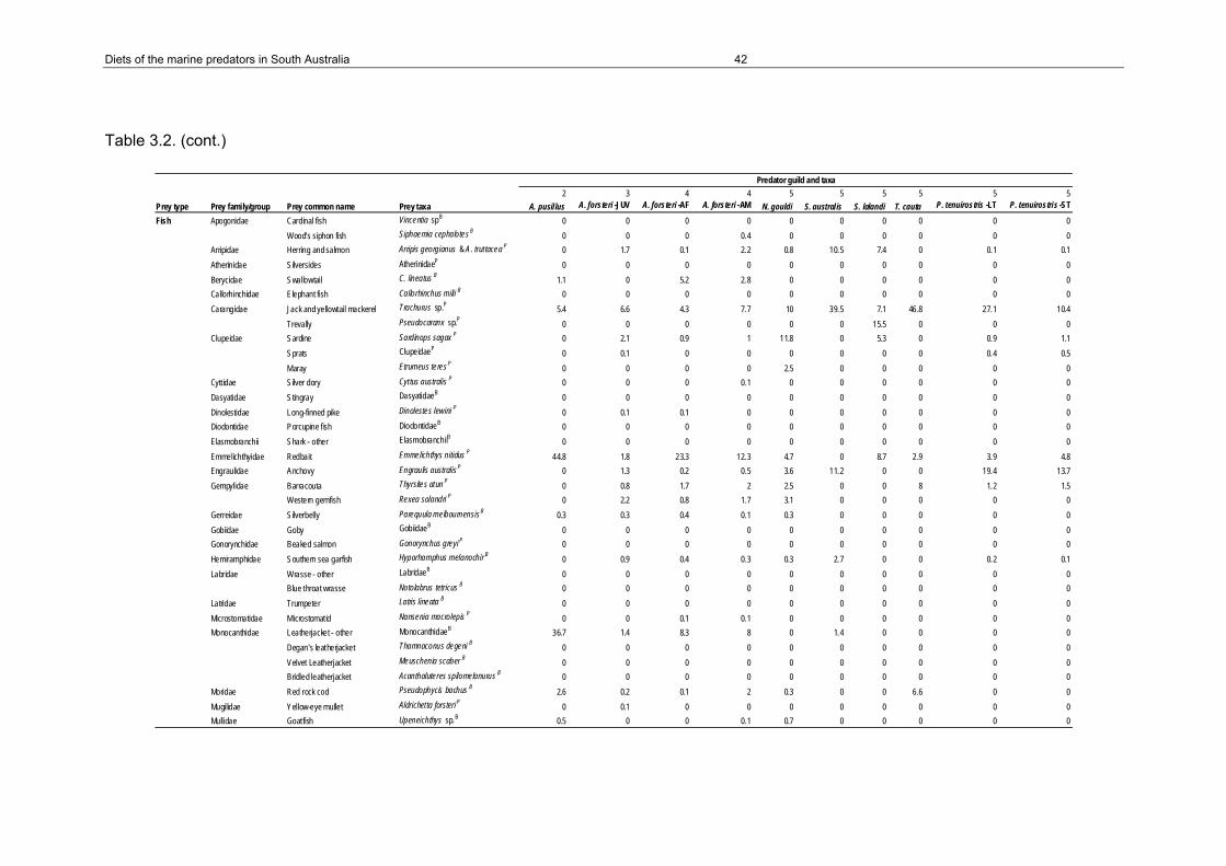
Diets of the marine predators in South Australia 42
Table 3.2. (cont.)
2 3 4 4 5 5 5 5 5 5Prey type Prey family/group Prey common name Prey taxa A. pusil lus A. forsteri -JUV A. forsteri -AF A. forsteri -AM N. gouldi S. australis S. lalandi T. cauta P. tenuirostris -LT P. tenuirostris -ST
Fish Apogonidae Cardinal fish Vincentia spB 0 0 0 0 0 0 0 0 0 0 Wood's siphon fish Siphaemia cephalotes B 0 0 0 0.4 0 0 0 0 0 0 Arripidae Herring and salmon Arripis georgianus & A. truttacea P 0 1.7 0.1 2.2 0.8 10.5 7.4 0 0.1 0.1 Atherinidae Silversides AtherinidaeP 0 0 0 0 0 0 0 0 0 0 Berycidae Swallowtail C. lineatus B 1.1 0 5.2 2.8 0 0 0 0 0 0 Callorhinchidae Elephant fish Callorhinchus milii B 0 0 0 0 0 0 0 0 0 0 Carangidae Jack and yellowtail mackerel Trachurus sp.P 5.4 6.6 4.3 7.7 10 39.5 7.1 46.8 27.1 10.4 Trevally Pseudocaranx sp.P 0 0 0 0 0 0 15.5 0 0 0
Clupeidae Sardine Sardinops sagax P 0 2.1 0.9 1 11.8 0 5.3 0 0.9 1.1 Sprats ClupeidaeP 0 0.1 0 0 0 0 0 0 0.4 0.5 Maray Etrumeus teresP 0 0 0 0 2.5 0 0 0 0 0 Cyttidae Silver dory Cyttus australis P 0 0 0 0.1 0 0 0 0 0 0 Dasyatidae Stingray DasyatidaeB 0 0 0 0 0 0 0 0 0 0 Dinolestidae Long-finned pike Dinolestes lewini P 0 0.1 0.1 0 0 0 0 0 0 0 Diodontidae Porcupine fish DiodontidaeB 0 0 0 0 0 0 0 0 0 0 Elasmobranchii Shark - other ElasmobranchiiB 0 0 0 0 0 0 0 0 0 0 Emmelichthyidae Redbait Emmelichthys nitidus P 44.8 1.8 23.3 12.3 4.7 0 8.7 2.9 3.9 4.8 Engraulidae Anchovy Engraulis australisP 0 1.3 0.2 0.5 3.6 11.2 0 0 19.4 13.7 Gempylidae Barracouta Thyrsites atun P 0 0.8 1.7 2 2.5 0 0 8 1.2 1.5 Western gemfish Rexea solandri P 0 2.2 0.8 1.7 3.1 0 0 0 0 0 Gerreidae Silverbelly Parequula melbournensisB 0.3 0.3 0.4 0.1 0.3 0 0 0 0 0 Gobiidae Goby GobiidaeB 0 0 0 0 0 0 0 0 0 0 Gonorynchidae Beaked salmon Gonorynchus greyi P 0 0 0 0 0 0 0 0 0 0 Hemiramphidae Southern sea garfish Hyporhamphus melanochir B 0 0.9 0.4 0.3 0.3 2.7 0 0 0.2 0.1 Labridae Wrasse - other LabridaeB 0 0 0 0 0 0 0 0 0 0 Blue throat wrasse Notolabrus tetricus B 0 0 0 0 0 0 0 0 0 0 Latridae Trumpeter Latris lineata B 0 0 0 0 0 0 0 0 0 0 Microstomatidae Microstomatid Nansenia macrolepis P 0 0 0.1 0.1 0 0 0 0 0 0 Monocanthidae Leatherjacket - other MonocanthidaeB 36.7 1.4 8.3 8 0 1.4 0 0 0 0 Degan's leatherjacket Thamnaconus degeni B 0 0 0 0 0 0 0 0 0 0 Velvet Leatherjacket Meuschenia scaber B 0 0 0 0 0 0 0 0 0 0 Bridled leatherjacket Acanthaluteres spilomelanurus B 0 0 0 0 0 0 0 0 0 0 Moridae Red rock cod Pseudophycis bachus B 2.6 0.2 0.1 2 0.3 0 0 6.6 0 0 Mugilidae Yellow-eye mullet Aldrichetta forsteri P 0 0.1 0 0 0 0 0 0 0 0 Mullidae Goatfish Upeneichthys sp.B 0.5 0 0 0.1 0.7 0 0 0 0 0
Predator guild and taxa

Diets of the marine predators in South Australia 43
Table 3.2. (cont.)
2 3 4 4 5 5 5 5 5 5Prey type Prey family/group Prey common name Prey taxa A. pusillus A. forsteri -JUV A. forsteri -AF A. forsteri -AM N. gouldi S. australis S. lalandi T. cauta P. tenuirostris -LT P. tenuirostris -ST
Fish (cont.) Myctophidae Lanternf ish Symbolophorus sp.P 0.1 10.9 0.9 0.4 0 0 0 0 0 0 Lanternf ish MyctophidaeP 0 0 0 0 0 0 0 0 4.8 0.8 Belted lanternfish Electrona paucirastra P 0 0 0 0 0 0 0 0 4 0.6 Jensen's lanternfish Diaphus jenseni P 0 0 0 0 0 0 0 0 3.7 0.6 Carlsberg's lanternfish, Electrona carlsbergi P 0 0 0 0 0 0 0 0 3.5 0.6 Lanternf ish Krefft ichthys anderssoni P 0 0 0 0 0 0 0 0 2.7 0.4 Lanternf ish Gymnoscopelus robustusP 0 1.1 0.2 0.2 0 0 0 0 0 0 Neosebastidae Gurnard perch NeosebastidaeB 0 0 0 0 0 0 0 0 0 0 Notocheiridae Surf sardine Iso rhothophilus P 0 0 0 0 0.7 0 0 0 0 0 Odacidae Weed whit ing OdacidaeB 0 0 0 0 0 0 0 0 0 0 Oreosomatidae Smooth oreo Pseudocyttus maculatus P 0 0 0 0 0 0 0 0 0 0 Pempherididae Bullseye Pempheris sp.B 0 16.7 0.7 0.2 0 14.3 0 0 0 0 Platycephalidae Flathead Neoplatycephalus spB 0 0 1.2 0 0 9.9 0 0 0 0 Tiger flathead Neoplatycephalus richardsoni B 2 0 0.1 0.2 0 0 0 0 0 0 Scomberesocidae Saury Scomberesox saurusP 0 0 0.1 0 0 0 0 0 0 0 Scombridae Blue Mackerel Scomber australasicus P 0 0 0.1 0.1 0.2 0 8.9 0 0.4 0.6 Southern bluefin tuna Thunnus maccoyii P 0 0 0 0 0 0 0 0 0 0 Scorpaenidae Scorpionfish ScorpaenidaeB 0 0 0 0 0 0 0 0 0 0 Scorpididae Sweep Scorpis aequipinnis P 0 0 0 0 0 0 0 0 0 0 Seriolella Spotted warehou Seriolella punctata P 0 0 0.1 0 0 0 0 0 0 0 Serranidae Perch SerranidaeB 0 0 0 0 0 0 0 0 0 0 Sillaginidae Eastern school whiting Sillago flindersi B 0.3 0 0.4 0.1 0 0 0 0 0 0 Western school whiting Sillago bassensis B 0 0.2 0.2 0.3 0 0 0 0 0 0 King George whit ing Sillaginodes puncata B 0 0 0 0 0 0 0 0 0 0 Sparidae Snapper Chrysophrys auratus B 0 0 0 0 0 0 0 0 0 0 Sygnathidae Pipefish SygnathidaeB 0 0 0 0 0 0 0 0 0 0 Sea horse SygnathidaeB 0 0 0 0 0 0 0 0 0 0 Terapontidae Western striped trumpeter Pelates octolineatus B 0 0 0 0 0 0 0 0 0 0 Tetraodontidae Toads TetraodontidaeB 0 0 0 0 0 0 0 0 0 0 Trachichthyidae Roughy TrachichthyidaeP 0 0 0 0 0.8 0 0 0 0 0 Unknown fish eggs Unknown fish eggs Unknown fish eggsP 0 0 0 0 0 0 0 0 0 0 Uranoscopidae Stargazer UranoscopidaeB 0.7 0.1 0 0.1 0 0 0 0 0 0
Predator guild and taxa

Diets of the marine predators in South Australia 44
Table 3.2. (cont.)
2 3 4 4 5 5 5 5 5 5Prey type Prey family/group Prey common name Prey taxa A. pusillus A. forsteri -JUV A. forsteri -AF A. forsteri -AM N. gouldi S. australis S. lalandi T. cauta P. tenuirostris -LT P. tenuirostris -ST
Cephalopod Argonautidae Southern argonaut Argonauta nodosa P 0 0 0 0 0 0 0 0.4 0 0 Histioteuthidae Jewel squid Histioteuthis sp.P 0.2 0 0.1 0 0 0 0 0 0 0 Loliginidae Calamary squid Sepioteuthis australisP 0 0.3 0.4 0.2 1.1 0 0 0 0 0 Octopodidae Octopus - other OctopodidaeB 0.5 0 0 0.1 0 2.1 0 0 0 0 Maori octopus Octopus maorum B 0 0 0 0.1 0 0 0 0 0 0 Southern keeled octopus Octopus berrima B 0 0 0 0 0 0 0 0 0 0 Ommastrephidae Gould's squid Nototodarus gouldi P 0.3 14 15.9 11.6 21.4 0 26.9 8.1 11.6 6.2 Arrow squids OmmastrephidaeP 4.3 22.7 12.2 10.9 0 0 0 0 1.7 0.6 Southern Ocean arrow squid Todarodes filippovae P 0 2.3 4.1 1.5 0 0 0 0 0 0 Sepiidae Giant cuttlefish Sepia apama B 0 0 0 0.1 0 0 0 26.7 0 0 Cuttlefish - other Sepia sp.B 0.2 0 0 0 0.9 0 4.6 0 0 0 Sepiolidae Southern dumpling squid Euprymna tasmanica B 0 0 0 0 0 0 0 0 0 0Crustacean Amphipoda Amphipod AmphipodaP 0 0 0 0 3.7 0 0 0 0.3 12.9 Crustacean - other Crustacean - other CrustaceanP 0 0 0 0 0.4 2.4 0 0 1.8 4.7 Decapoda Decapod DecapodaP 0 0 0 0 0 2.4 0 0 0 0 Euphausiidae Krill Nyctiphanes australis P 0 0 0 0 25.8 0 15.6 0.1 11 39.2 Isopoda Isopod IsopodaP 0 0 0 0 0 0 0 0 1.2 0 Maxillopoda Copepod MaxillopodaP 0 0 0 0 0 0 0 0 0.1 0.3 Ostracoda Ostracod OstracodaP 0 0 0 0 0 0 0 0 0 0 Palinuridae Southern rock lobster Jasus edwardsii B 0 0 0 0 0 0 0 0 0 0 Pandalidae Pandalid prawn PandalidaeB 0 0 0 0 0.4 0 0 0 0 0 Penaeidae Western king prawn Melicertus latisulcatus B 0 0 0 0 0 3.6 0 0 0 0 Southern velvet shrimp Metapenaeopsis palmensisB 0 0 0.1 0 0 0 0 0 0 0Bird Procellariidae Shearwater Puffinus sp.P 0 0.3 3.6 2.4 0 0 0 0 0 0 Seabird - other Seabird - other Seabird - otherP 0 0 0 0.1 0 0 0 0 0 0 Spheniscidae Little penguin Eudyptula minor P 0 11.8 13.7 30.1 0 0 0 0 0 0Other Donacidae Cockle Plebidonax deltoidesB 0 0 0 0 0 0 0 0 0 0 Insecta Insect InsectaT 0 0 0 0 0 0 0 0 0 0.3 Mollusca Mullusc MolluscaB 0 0 0 0 0.1 0 0 0 0 0 Nereididae Nereid Worm NereididaeP 0 0 0 0 3.9 0 0 0 0 0 Plant - marine Plant - marine Plant - marineB 0 0 0 0 0 0 0 0 0 0 Plant - terrestrial Plant - terrestrial Plant - terrestrialT 0 0 0 0 0 0 0 0 0 0 Polychaeta Worm PolychaetaP 0 0 0 0 0 0 0 0 0 0 Salpidae Salp SalpidaeP 0 0 0 0 0 0 0 0.4 0 0
Predator guild and taxa

Diets of the marine predators in South Australia 45
Table 3.2. (cont.)
6 6 6 6 6 6 7Prey type Prey family/group Prey common name Prey taxa N. cinerea P. glauca C. brachyurus phyrna sp. I. oxyrinchus T. aduncus C. novaehollandiaeFish Apogonidae Cardinal fish Vincentia spB 0.1 0 0 0 0 20.7 0 Wood's siphon fish Siphaemia cephalotesB 0 0 0 0 0 0 0 Arripidae Herring and salmon Arripis georgianus & A. truttacea P 0.2 0 0 0 0 0.1 0.1 Atherinidae Silversides AtherinidaeP 0 0 0 0 0 0 0 Berycidae Swallowtail C. lineatus B 1.6 0 0 0.2 0 0.1 0 Callorhinchidae Elephant fish Callorhinchus milii B 0 0 0 0 0 0 0 Carangidae Jack and yellowtail mackerel Trachurus sp.P 0.8 0 0 1.9 0.1 1.5 0 Trevally Pseudocaranx sp.P 0 0 0 0 0 0.9 0
Clupeidae Sardine Sardinops sagax P 0.1 0 35.4 0 0 2.1 2.8 Sprats ClupeidaeP 0 0 0 0 0 0 0.1 Maray Etrumeus teresP 0 0 0 0 0 0 0 Cytt idae Silver dory Cyttus australis P 0 0 0 0 0 0 0 Dasyatidae Stingray DasyatidaeB 0.4 0 1.1 0 0 0 0 Dinolestidae Long-finned pike Dinolestes lewini P 0 0 0 0 0 0 0 Diodontidae Porcupine f ish DiodontidaeB 0 0 0 0 0 0 0 Elasmobranchii Shark - other ElasmobranchiiB 0.2 0 2.2 0 0 0 0 Emmelichthyidae Redbait Emmelichthys nitidus P 0 0 0 0 0 0 0 Engraulidae Anchovy Engraulis australisP 0 0 0.3 0.3 0 0 0 Gempylidae Barracouta Thyrsites atun P 0.1 0 0 0 0 0 0 Western gemfish Rexea solandri P 0 0 0 0 0 0 0 Gerreidae Silverbelly Parequula melbournensisB 1.6 0 0 0 0 1.4 1 Gobiidae Goby GobiidaeB 0 0 0 0 0 1.5 0 Gonorynchidae Beaked salmon Gonorynchus greyi P 0 0 0 0 0 0 0 Hemiramphidae Southern sea garfish Hyporhamphus melanochir B 0 0 0 0 0 0 0.3 Labridae Wrasse - other LabridaeB 0.8 0 0.3 0 0 0 14.7 Blue throat wrasse Notolabrus tetricus B 3.8 0 0 0 0 0 0 Latridae Trumpeter Latris lineata B 0 0 0 0 0 0.2 0 Microstomatidae Microstomatid Nansenia macrolepis P 0 0 0 0 0 0 0 Monocanthidae Leatherjacket - other MonocanthidaeB 2.4 0 0 0 0 0 0 Degan's leatherjacket Thamnaconus degeni B 0 0 0.1 0 0 0 29.1 Velvet Leatherjacket Meuschenia scaber B 3.7 0 0 0 0 0 0 Bridled leatherjacket Acanthaluteres spilomelanurus B 0 0 0 0 0 0 0 Moridae Red rock cod Pseudophycis bachus B 0.8 0 0 0 0 0 0 Mugilidae Yellow-eye mullet Aldrichetta forsteri P 0 0 0 0 0 0 0 Mullidae Goatfish Upeneichthys sp.B 1.5 0 0 0 0 0 1.2
Predator guild and taxa

Diets of the marine predators in South Australia 46
Table 3.2. (cont.)
6 6 6 6 6 6 7Prey type Prey family/group Prey common name Prey taxa N. cinerea P. glauca C. brachyurus phyrna sp. I . oxyrinchus T. aduncus C. novaehollandiaeFish (cont.) Myctophidae Lanternf ish Symbolophorus sp.P 0 0 0 0 0 0 0 Lanternf ish MyctophidaeP 0 0 0 0 0 0 0 Belted lanternfish Electrona paucirastra P 0 0 0 0 0 0 0 Jensen's lanternfish Diaphus jenseni P 0 0 0 0 0 0 0 Carlsberg's lanternfish, Electrona carlsbergi P 0 0 0 0 0 0 0 Lanternf ish Krefft ichthys anderssoni P 0 0 0 0 0 0 0 Lanternf ish Gymnoscopelus robustusP 0 0 0 0 0 0 0 Neosebastidae Gurnard perch NeosebastidaeB 2.1 0 0 0 0 0 0 Notocheiridae Surf sardine Iso rhothophilus P 0 0 0 0 0 0 0 Odacidae Weed whit ing OdacidaeB 0.1 0 0 0 0 0.2 0 Oreosomatidae Smooth oreo Pseudocyttus maculatus P 0 0 0 0 0 0 0 Pempherididae Bullseye Pempheris sp.B 0.2 0 0 0 0 1.2 0.2 Platycephalidae Flathead Neoplatycephalus spB 0.8 0 0 0 0 0.2 1.3 Tiger flathead Neoplatycephalus richardsoni B 2.7 0 0 0 0 0 0 Scomberesocidae Saury Scomberesox saurusP 0 0 0 0 0 0 0 Scombridae Blue Mackerel Scomber australasicus P 0 28.4 0.1 0 0 0 0 Southern bluefin tuna Thunnus maccoyii P 0 0 0 7.8 74.1 0 0 Scorpaenidae Scorpionfish ScorpaenidaeB 0 0 0 0 0 0.3 0 Scorpididae Sweep Scorpis aequipinnis P 0 0 0 0 0 0.7 0 Seriolella Spotted warehou Seriolella punctata P 0 0 0 0 0 0 0 Serranidae Perch SerranidaeB 1.5 0 0 0 0 1.9 0 Sillaginidae Eastern school whiting Sillago flindersi B 0.4 0 0 0 0 0 0 Western school whiting Sillago bassensis B 0.2 0 0 0 0 0 0 King George whit ing Sillaginodes puncata B 0.1 0 0 0 0 0.7 0 Sparidae Snapper Chrysophrys auratus B 0 0 0 0 0 0 0 Sygnathidae Pipefish SygnathidaeB 0 0 0 0 0 0 0 Sea horse SygnathidaeB 0 0 0 0.1 0 0.2 0 Terapontidae Western striped trumpeter Pelates octolineatus B 0 0 0 0 0 4.1 0 Tetraodontidae Toads TetraodontidaeB 0 0 0 0 0 0 0 Trachichthyidae Roughy TrachichthyidaeP 0 0 0 0 0 0 0 Unknown fish eggs Unknown fish eggs Unknown fish eggsP 0 0 0 0 0 0 0 Uranoscopidae Stargazer UranoscopidaeB 0 0 0 0 0 0 0
Predator guild and taxa

Diets of the marine predators in South Australia 47
Table 3.2. (cont.)
6 6 6 6 6 6 7Prey type Prey family/group Prey common name Prey taxa N. cinerea P. glauca C. brachyurus phyrna sp. I . oxyrinchus T. aduncus C. novaehollandiaeCephalopod Argonautidae Southern argonaut Argonauta nodosa P 0 0 0 0 0 0 0 Histioteuthidae Jewel squid Histioteuthis sp.P 0 0 0 0 0 0 0 Loliginidae Calamary squid Sepioteuthis australisP 14.8 0 29.5 39.5 0 13.4 0.1 Octopodidae Octopus - other OctopodidaeB 23.4 0 8.1 0 0 28.5 0.5 Maori octopus Octopus maorum B 4.3 11.9 0 0 0 0 0 Southern keeled octopus Octopus berrima B 2.5 0 0 0 0 0 0 Ommastrephidae Gould's squid Nototodarus gouldi P 1.2 29.9 9.4 24.6 15.9 0 0.2 Arrow squids OmmastrephidaeP 3.5 0 0 0 0 0 0 Southern Ocean arrow squid Todarodes filippovae P 0 17.9 5.4 3.5 9.9 0 0 Sepiidae Giant cuttlef ish Sepia apama B 15.3 11.9 0 12.7 0 3.6 0 Cuttlefish - other Sepia sp.B 3.2 0 8.1 8.5 0 16.5 2.3 Sepiolidae Southern dumpling squid Euprymna tasmanica B 0.6 0 0 0 0 0 0Crustacean Amphipoda Amphipod AmphipodaP 0 0 0 0 0 0 0 Crustacean - other Crustacean - other CrustaceanP 2.2 0 0 0 0 0 5 Decapoda Decapod DecapodaP 0 0 0 0.9 0 0 0 Euphausiidae Krill Nyctiphanes australis P 0 0 0 0 0 0 0 Isopoda Isopod IsopodaP 0 0 0 0 0 0 0 Maxillopoda Copepod MaxillopodaP 0 0 0 0 0 0 0 Ostracoda Ostracod OstracodaP 0 0 0 0 0 0 0 Palinuridae Southern rock lobster Jasus edwardsii B 2.1 0 0 0 0 0 0 Pandalidae Pandalid prawn PandalidaeB 0 0 0 0 0 0 0 Penaeidae Western king prawn Melicertus latisulcatus B 0.4 0 0 0 0 0 0 Southern velvet shrimp Metapenaeopsis palmensisB 0 0 0 0 0 0 0Bird Procellariidae Shearwater Puffinus sp.P 0 0 0 0 0 0 0 Seabird - other Seabird - other Seabird - otherP 0 0 0 0 0 0 1.3 Spheniscidae Little penguin Eudyptula minor P 0.3 0 0 0 0 0 0Other Donacidae Cockle Plebidonax deltoidesB 0 0 0 0 0 0 1.7 Insecta Insect InsectaT 0 0 0 0 0 0 5.2 Mollusca Mullusc MolluscaB 0 0 0 0 0 0 3.5 Nereididae Nereid Worm NereididaeP 0 0 0 0 0 0 0 Plant - marine Plant - marine Plant - marineB 0 0 0 0 0 0 9.4 Plant - terrestrial Plant - terrestrial Plant - terrestrialT 0 0 0 0 0 0 20 Polychaeta Worm PolychaetaP 0 0 0 0 0 0 0 Salpidae Salp SalpidaeP 0 0 0 0 0 0 0
Predator guild and taxa

Diets of the marine predators in South Australia 48
Table 3.2. (cont.)
8 8 8 8 8 8 8 8 8Prey type Prey family/group Prey common name Prey taxa E. australis S. australasicus B. musculus T. declivis E. teres E. nitidus S. sagax S. robustus C. lineatusFish Apogonidae Cardinal f ish Vincentia spB 0 0 0 0 0 0 0 0 0 Wood's siphon fish Siphaemia cephalotesB 0 0 0 0 0 0 0 0 0 Arripidae Herring and salmon Arripis georgianus & A. truttacea P 0 0 0 0 0 0 0 0 0 Atherinidae Silversides AtherinidaeP 0 0 0 0 0 0 0 0 0 Berycidae Swallowtail C. lineatusB 0 0 0 0 0 0 0 0 0 Callorhinchidae Elephant fish Callorhinchus milii B 0 0 0 0 0 0 0 0 0 Carangidae Jack and yellowtail mackerel Trachurus sp.P 0 0 0 0 0 0 0 0 0 Trevally Pseudocaranx sp.P 0 0 0 0 0 0 0 0 0
Clupeidae Sardine Sardinops sagax P 0 0 0 0 0 0 0 0 0 Sprats ClupeidaeP 0 0 0 0 0 0 0 0 0 Maray Etrumeus teres P 0 0 0 0 0 0 0 0 0 Cyttidae Silver dory Cyttus australis P 0 0 0 0 0 0 0 0 0 Dasyatidae Stingray Dasyat idaeB 0 0 0 0 0 0 0 0 0 Dinolestidae Long-finned pike Dinolestes lewini P 0 0 0 0 0 0 0 0 0 Diodontidae Porcupine fish DiodontidaeB 0 0 0 0 0 0 0 0 0 Elasmobranchii Shark - other ElasmobranchiiB 0 0 0 0 0 0 0 0 0 Emmelichthyidae Redbait Emmelichthys nitidusP 0 0 0 0 0 0 0 0 0 Engraulidae Anchovy Engraulis australis P 0 0 0 0 0 0 0 0 0 Gempylidae Barracouta Thyrsites atun P 0 0 0 0 0 0 0 0 0 Western gemfish Rexea solandri P 0 0 0 0 0 0 0 0 0 Gerreidae Silverbelly Parequula melbournensisB 0 0 0 0 0 0 0 0 0 Gobiidae Goby GobiidaeB 0 0 0 0 0 0 0 0 0 Gonorynchidae Beaked salmon Gonorynchus greyi P 0 0 0 0 0 0 0 0 0 Hemiramphidae Southern sea garfish Hyporhamphus melanochir B 0 0 0 0 0 0 0 0 0 Labridae Wrasse - other LabridaeB 0 0 0 0 0 0 0 0 0 Blue throat wrasse Notolabrus tetricus B 0 0 0 0 0 0 0 0 0 Latridae Trumpeter Latris lineata B 0 0 0 0 0 0 0 0 0 Microstomatidae Microstomatid Nansenia macrolepisP 0 0 0 0 0 0 0 0 0 Monocanthidae Leatherjacket - other MonocanthidaeB 0 0 0 0 0 0 0 0 0 Degan's leatherjacket Thamnaconus degeni B 0 0 0 0 0 0 0 0 0 Velvet Leatherjacket Meuschenia scaber B 0 0 0 0 0 0 0 0 0 Bridled leatherjacket Acanthaluteres spilomelanurus B 0 0 0 0 0 0 0 0 0 Moridae Red rock cod Pseudophycis bachusB 0 0 0 0 0 0 0 0 0 Mugilidae Yellow-eye mullet Aldrichetta forsteri P 0 0 0 0 0 0 0 0 0 Mullidae Goatfish Upeneichthys sp.B 0 0 0 0 0 0 0 0 0
Predator guild and taxa

Diets of the marine predators in South Australia 49
Table 3.2. (cont.)
8 8 8 8 8 8 8 8 8Prey type Prey family/group Prey common name Prey taxa E. australis S. australasicus B. musculus T. declivis E. teres E. nitidus S. sagax S. robustus C. lineatusFish (cont.) Myctophidae Lanternfish Symbolophorus sp.P 0 0 0 0 0 0 0 0 0 Lanternfish MyctophidaeP 0 0 0 0 0 0 0 0 0 Belted lanternfish Electrona paucirastra P 0 0 0 0 0 0 0 0 0 Jensen's lanternfish Diaphus jenseni P 0 0 0 0 0 0 0 0 0 Carlsberg's lanternfish, Electrona carlsbergi P 0 0 0 0 0 0 0 0 0 Lanternfish Krefftichthys anderssoni P 0 0 0 0 0 0 0 0 0 Lanternfish Gymnoscopelus robustus P 0 0 0 0 0 0 0 0 0 Neosebastidae Gurnard perch NeosebastidaeB 0 0 0 0 0 0 0 0 0 Notocheiridae Surf sardine Iso rhothophilus P 0 0 0 0 0 0 0 0 0 Odacidae Weed whiting OdacidaeB 0 0 0 0 0 0 0 0 0 Oreosomatidae Smooth oreo Pseudocyttus maculatus P 0 0 0 0 0 0 0 0 0 Pempherididae Bullseye Pempheris sp.B 0 0 0 0 0 0 0 0 0 Platycephalidae Flathead Neoplatycephalus spB 0 0 0 0 0 0 0 0 0 Tiger flathead Neoplatycephalus richardsoni B 0 0 0 0 0 0 0 0 0 Scomberesocidae Saury Scomberesox saurusP 0 0 0 0 0 0 0 0 0 Scombridae Blue Mackerel Scomber australasicus P 0 0 0 0 0 0 0 0 0 Southern bluefin tuna Thunnus maccoyii P 0 0 0 0 0 0 0 0 0 Scorpaenidae Scorpionfish ScorpaenidaeB 0 0 0 0 0 0 0 0 0 Scorpididae Sweep Scorpis aequipinnis P 0 0 0 0 0 0 0 0 0 Seriolella Spotted warehou Seriolella punctata P 0 0 0 0 0 0 0 0 0 Serranidae Perch SerranidaeB 0 0 0 0 0 0 0 0 0 Sillaginidae Eastern school whiting Sillago flindersi B 0 0 0 0 0 0 0 0 0 Western school whit ing Sillago bassensisB 0 0 0 0 0 0 0 0 0 King George whiting Sillaginodes puncata B 0 0 0 0 0 0 0 0 0 Sparidae Snapper Chrysophrys auratus B 0 0 0 0 0 0 0 0 0 Sygnathidae Pipefish SygnathidaeB 0 0 0 0 0 0 0 0 0 Sea horse SygnathidaeB 0 0 0 0 0 0 0 0 0 Terapontidae Western striped trumpeter Pelates octolineatus B 0 0 0 0 0 0 0 0 0 Tetraodontidae Toads TetraodontidaeB 0 0 0 0 0 0 0 0 0 Trachichthyidae Roughy TrachichthyidaeP 0 0 0 0 0 0 0 0 0 Unknown fish eggs Unknown fish eggs Unknown fish eggsP 6.8 18.8 0 2.4 1.9 0.4 1.6 0 0 Uranoscopidae Stargazer UranoscopidaeB 0 0 0 0 0 0 0 0 0
Predator guild and taxa

Diets of the marine predators in South Australia 50
8 8 8 8 8 8 8 8 8Prey type Prey family/group Prey common name Prey taxa E. australis S. australasicus B. musculus T. declivis E. teres E. nitidus S. sagax S. robustus C. lineatusCephalopod Argonautidae Southern argonaut Argonauta nodosa P 0 0 0 0 0 0 0 0 0 Histioteuthidae Jewel squid Histioteuthis sp.P 0 0 0 0 0 0 0 0 0 Loliginidae Calamary squid Sepioteuthis australisP 0 0 0 0 0 0 0 0 0 Octopodidae Octopus - other OctopodidaeB 0 0 0 0 0 0 0 0 0 Maori octopus Octopus maorum B 0 0 0 0 0 0 0 0 0 Southern keeled octopus Octopus berrima B 0 0 0 0 0 0 0 0 0 Ommastrephidae Gould's squid Nototodarus gouldi P 0 0 0 0 0 0 0 0 0 Arrow squids OmmastrephidaeP 0 0 0 0 0 0 0 0 0 Southern Ocean arrow squid Todarodes f ilippovae P 0 0 0 0 0 0 0 0 0 Sepiidae Giant cuttlefish Sepia apama B 0 0 0 0 0 0 0 0 0 Cuttlefish - other Sepia sp.B 0 0 0 0 0 0 0 0 0 Sepiolidae Southern dumpling squid Euprymna tasmanica B 0 0 0 0 0 0 0 0 0Crustacean Amphipoda Amphipod AmphipodaP 0 0 0 0 0 0 0 0 0 Crustacean - other Crustacean - other CrustaceanP 47.2 14.9 0 11.7 5.5 20.2 28.4 86.5 0 Decapoda Decapod DecapodaP 0 0 0 0 0 0.1 0 0 0 Euphausiidae Krill Nyct iphanes australisP 46.0 61.7 100 72.6 92.6 55.8 65.3 0 91.3 Isopoda Isopod IsopodaP 0 0 0 0 0 0 0 0 8.7 Maxillopoda Copepod MaxillopodaP 0 0 0 0 0 0.6 0 0 0 Ostracoda Ostracod OstracodaP 0 0 0 0 0 0 1.1 0 0 Palinuridae Southern rock lobster Jasus edwardsii B 0 0 0 0 0 0 0 0 0 Pandalidae Pandalid prawn PandalidaeB 0 0 0 0 0 0 0 0 0 Penaeidae Western king prawn Melicertus latisulcatusB 0 0 0 0 0 0 0 0 0 Southern velvet shrimp Metapenaeopsis palmensis B 0 0 0 0 0 0 0 0 0Bird Procellariidae Shearwater Puffinus sp.P 0 0 0 0 0 0 0 0 0 Seabird - other Seabird - other Seabird - otherP 0 0 0 0 0 0 0 0 0 Spheniscidae Little penguin Eudyptula minor P 0 0 0 0 0 0 0 0 0Other Donacidae Cockle Plebidonax deltoides B 0 0 0 0 0 0 0 0 0 Insecta Insect InsectaT 0 0 0 0 0 0 0 0 0 Mollusca Mullusc MolluscaB 0 2.4 0 0.6 0 19.3 0.5 0 0 Nereididae Nereid Worm NereididaeP 0 0 0 0 0 0 0 0 0 Plant - marine Plant - marine Plant - marineB 0 1.6 0 0 0 1.7 0.2 13.5 0 Plant - terrestrial Plant - terrestrial Plant - terrestrialT 0 0 0 0 0 0 0 0 0 Polychaeta Worm PolychaetaP 0 0 0 11.4 0 0.8 0 0 0 Salpidae Salp SalpidaeP 0 0.6 0 1.3 0 1.1 2.9 0 0
Predator guild and taxa
Table 3.2. (cont.)

Diets of the marine predators in South Australia 51
Guilds based on diet of predator groups
SIMPROF detected 8 significantly different guilds among the 37 predator groups, based on
similarities in their diets (P < 0.05, Figure 3.1). Because the diet data are weighted by the
number and size of prey consumed, these guilds reflect differences and similarities in the
relative prey mass taken by each group. The average number of predator groups in each
guild was 4.6 ± 4.0, with a maximum of 11. Three guilds contained a single predator group,
indicating that their diets were significantly different from all other predator groups in the
study (A. p. doriferus adult males, A. forsteri juveniles and C. novaehollandiae, Figure 3.1).
The average similarity level between different guilds was 20% ± 18%. Five of the guilds
were discerned with diet similarities of less than 25%, indicating that 75% of their diets
comprised either different prey species or different proportions of the same prey. The 3
remaining guilds were discerned with diet similarities between 30%-54%, which were
predator groups of A. p. doriferus and the age/sex groups of A. forsteri. The average of
within-guild similarity could be calculated for guilds 1, 4, 5, 6 and 8, because they had more
than one predator group, and it was 33.8%, 73.5%, 34.5%, 24.3% and 57.7% respectively
(average 44.8% ± 20.2%).
SIMPER determined how much each prey taxon accounted for the differences between the
guilds (Table 3.3). Prey that accounted for these differences do not indicate that a guild was
its sole consumer, but rather that such prey were relatively important for one guild compared
to the others. Overall, the prey species that accounted for the differences between the guilds
(Table 3.3) comprised an average of 71.8% ± 13.8% of each guild’s total consumption. Guild
1 (11 predator groups) was largely discerned by its consumption of S. sagax, E. australis
and Pempheris sp. Guild 2 (A. p. doriferus adult males) was unique in its high consumption
of E. nitidus and Monocanthidae. Guild 3 (A. forsteri juveniles) was distinguished by
consumption of Ommastrephidae, Pempheris sp. and N. gouldi. Guild 4 (Adult male and
female A. forsteri) was distinguished from other predator groups by the consumption of E.
minor, E. nitidus and N. gouldi. Guild 5 (6 predator groups) was distinguished by its
consumption of Trachurus sp., N. australis, N. gouldi and E. australis. Guild 6 (6 predator
groups) used S. australis, T. maccoyii, N. gouldi and E. australis. Guild 7 (C.
novaehollandiae) was unique in its consumption of T. degeni, terrestrial plant material and
Labridae. Guild 8 (9 predator groups) was largely discerned by its consumption of N.
australis and other Crustaceans.

Diets of the marine predators in South Australia 52
Figure 3.1. Bray-Curtis similarity dendrogram of the diets of the 37 predator groups. Significantly different guilds are numbered 1-8 at the
bottom of the dendrogram (abbreviations: LT: long trip, ST: short trip, JUV: juvenile, AF: adult female, AM: adult male).

Diets of the marine predators in South Australia 53
Table 3.3. SIMPER results for prey taxa that contributed to the differences between guilds
(reported as SIMPER percentage). Only prey taxa that were consumed by a guild are
reported for that guild (prey taxa that were not consumed by a guild can contribute to
differences between guilds if the other guild used the taxa).
Guild Prey species SIMPER (%) Average proportion of diet1 Sardinops sagax 48 34.71 Engraulis australis 35 25.81 Pempheris sp. 10 7.61 Atherinidae 3 4.51 Nototodarus gouldi 2 4.81 Scomber australasicus 1 4.61 Thyrsites atun 1 4.0
Total 100 86.02 Emmelichthys nitidus 51 44.92 Monocanthidae 49 36.7
Total 100 81.603 Pempheris sp. 48 16.73 Ommastrephidae 38 22.53 Nototodarus gouldi 14 14.0
Total 100 53.24 Eudyptula minor 46 21.94 Emmelichthys nitidus 20 17.84 Nototodarus gouldi 19 13.74 Ommastrephidae 10 11.54 Monocanthidae 5 8.1
Total 100 73.15 Trachurus sp. 44 23.55 Nyctiphanes australis 27 15.25 Nototodarus gouldi 16 12.45 Engraulis australis 11 8.05 Sepia apama 2 4.5
Total 100 63.56 Sepioteuthis australis 32 16.26 Thunnus maccoyii 27 13.66 Nototodarus gouldi 19 13.56 Octopodidae 17 10.06 Sepia apama 5 7.2
Total 100 60.57 Thamnaconus degeni 57 29.17 Plant - terrestrial 25 20.07 Labridae 18 14.7
Total 100 63.88 Nyctiphanes australis 72 65.08 Crustacean 26 23.88 Fish eggs 2 3.5
Total 100 92.3
Grand mean ± SD 71.8 ± 13.8

Diets of the marine predators in South Australia 54
To determine the habitats that were typically used by the above guilds, we considered the
habitats used by their prey. Most prey were from PELAGIC habitats, with guild 7 (C.
novaehollandiae) being the only BENTHIC guild (65.2% of prey from benthic habitats). In
total, 33 predator groups were classified as PELAGIC, 4 were classified as BENTHIC and
none were classified as TERRESTRIAL (Table 3.4). As expected, the prey taxa used by the
33 PELAGIC predators were significantly different to the prey taxa used by the 4 BENTHIC
predators (R = 0.65, P = 0.026). Predator groups that were classified as PELAGIC (based
on proportional contribution of prey) were present in all guilds except guild 7 and BENTHIC
predator groups were present in guilds 2, 6 and 7. Guilds 1, 3, 4, 5 and 8 used more than
80% PELAGIC prey, and guilds 2 (55.1% PELAGIC) and 6 (62.7%) were also classified as
PELAGIC, but used relatively more BENTHIC prey (Table 3.4).

Diets of the marine predators in South Australia 55
Table 3.4. Habitat classification of each predator group, based on the habitat of the majority
of their prey and sorted by guilds.
Guild Predator Pelagic Benthic Terrestrial Habitat classification of predator1 A. vulpinus 100 0 0 Pelagic1 Sardine fishery 100 0 0 Pelagic1 Sarda australis 100 0 0 Pelagic1 T. atun 100 0 0 Pelagic1 T. maccoyii 99.8 0.2 0 Pelagic1 D. delphis 91.7 8.3 0 Pelagic1 E. minor 87.3 12.7 0 Pelagic1 M. serrator 82 18 0 Pelagic1 S. bergii 72.4 27.6 0 Pelagic1 A. truttacea 68.6 31.4 0 Pelagic1 S. novaehollandiae 41.5 58.5 0 Benthic
Average 85.8 (18.7) 14.2 (18.7) 0
2 A. pusillus doriferus 55.1 44.9 0 Pelagic
3 A. forsteri ‐JUV 80.1 19.9 0 Pelagic
4 A. forsteri ‐AM 85 15 0 Pelagic4 A. forsteri ‐AF 82.7 17.3 0 Pelagic
Average 83.9 (1.6) 16.1 (1.6) 0
5 P. tenuirostris ‐LT 99.8 0.2 0 Pelagic5 P. tenuirostris ‐ST 99.6 0.1 0.3 Pelagic5 N. gouldi 96.9 3.1 0 Pelagic5 S. lalandi 95.3 4.7 0 Pelagic5 T. cauta 66.7 33.3 0 Pelagic5 S. australis 66 34 0 Pelagic
Average 87.4 (16.4) 12.6 (16.4) 0
6 I. oxyrinchus 100 0 0 Pelagic6 C. brachyurus 80.2 19.8 0 Pelagic6 Sphyrna sp. 78.5 21.5 0 Pelagic6 P. glauca 76.1 23.9 0 Pelagic6 N. cinerea 23.2 76.8 0 Benthic6 T. aduncus 18.1 81.9 0 Benthic
Average 62.7 (33.7) 37.3 (33.7) 0
7 C. novaehollandiae 9.6 65.2 25.2 Benthic
8 B. musculus 100 0 0 Pelagic8 C. lineatus 100 0 0 Pelagic8 E. australis 100 0 0 Pelagic8 E. teres 100 0 0 Pelagic8 T. declivis 99.4 0.6 0 Pelagic8 S. sagax 99.3 0.7 0 Pelagic8 S. australasicus 96.1 3.9 0 Pelagic8 S. robustus 86.5 13.5 0 Pelagic8 E. nitidus 79 21 0 Pelagic
Average 95.6 (7.6) 4.4 (7.6) 0

Diets of the marine predators in South Australia 56
Discussion
Our study focussed on the diets of pelagic predators and our sampling was influenced by
their availability and the availability of datasets on the diet of other predators. Our study did
not include some ecologically-important species that occur in the region, because data on
their diets were not available. Four shark species that occur in the region, but are not part of
this study, are Carcharodon carcharias, Galeorhinus galeus, Carcharhinus obscurus and
Mustelus antarcticus, all of which are likely to compete with some of the predators in this
study (Simpfendorfer et al. 2001, Stevens 2005, Bruce et al. 2006). Seabirds such as
Pelagodroma marina, Thalassarche sp. and Puffinus carneipes (Copley 1996) and toothed
whales (Odontoceti) are also abundant in this region and studies from other regions indicate
that they are pelagic predators (e.g. Evans and Hindell 2004, Brooke 2004, Colabuono and
Vooren 2007). The prevalence of Myctophidae and Todarodes filippovae in the diets of
several predators indicates that they are ecologically important species. Nevertheless, they
were not included in this study because their diet data were not available.
Dietary differences among demographic groups of a single species are often profound,
indicating that some demographic groups should be separated in studies of ecosystem
processes (Polis 1984, reviewed in Andersson 1994, Isaac 2005). Our study indicated that
diets were not significantly different in 2 of the 3 age/sex classes of A. forsteri nor between
the two behavioural patterns analysed for P. tenuirostris. The diet of juvenile A. forsteri was
in a different guild to the adult age classes of that species, and Page et al. (2005) found
significant differences among all 3 of its age/sex classes. Our data indicate that in the broad
context of this study, diet differences between these age/sex classes are not as important as
inter-species differences. Despite this, our study would undoubtedly have benefited from the
inclusion of information about additional predator species and from splitting the different
age/sex classes of predator groups to identify ontogenetic diet shifts. Had we assessed
dietary differences among demographic groups of each species, it is likely that we would
have identified additional guilds, and so the results we have presented are likely to be over-
simplified. Nonetheless, we describe differences between the diets of 37 predator groups
that are ecologically and/or economically important in the region.
The patterns of resource partitioning identified in this study indicate that, based on their
diets, the 37 predator groups could be categorised into 8 guilds. We found that the guilds
could be discerned by 2-6 prey taxa and in all guilds these prey taxa comprised more than
half of their diets (Table 3.3). The guilds were split at similarity levels that averaged 20% ±
18%, which is at the lower end of dietary overlap values reported in other studies of

Diets of the marine predators in South Australia 57
resource competition in the marine environment (20%-70%, summarised in Garrison and
Link 2000). The average similarity level within guilds was 44.8% ± 20.2%, which is lower
than has been reported elsewhere (50%-80%, summarised in Garrison and Link 2000).
Together, these low similarity levels indicate that some of the predator groups are
specialists, with some groups using <5 prey taxa. This is an accurate reflection of the SA
sardine fishery, but is unlikely to be true for Sarda australis, A. vulpinus, B. musculus and I.
oxyrinchus, which have been reported to have broader diets elsewhere (e.g. Stillwell and
Kohler 1982, Collette and Nauen 1983, Preti et al. 2001, Sears 2002). Rather, the narrow
range of prey reported here is likely to be a result of the limited availability of diet samples,
and has most likely resulted in the lower than expected similarity levels. The apparent
specialist nature of E. australis, E. teres, S. robustus and C. lineatus, largely resulted from
their use of N. australis, but the similarity levels within their guild (Guild 8) may have been
inflated by the broad taxonomic groups used to classify their other prey (Daly 2007, Table
3.2). The difficulty in identifying the prey of predators that use small crustaceans is a
common problem in dietary studies (e.g. Braley 2010). Despite these shortcomings, our
analyses provide a practical picture of this complex and productive ecosystem.
Nyctiphanes australis and other pelagic crustaceans are the key links between primary
production and higher trophic levels in this pelagic ecosystem, as demonstrated by their
importance in the diets of the members of guilds 5 and 8. The small pelagic fishes from guild
8 and N. gouldi (guild 5) were, in turn, important prey for the predators in guilds 1, 2, 3, 4, 5
and 6, indicating that much of the energy flow in this ecosystem involves just 3 trophic levels
before it is available to top predators (2 trophic levels for some predator groups, including
the SA sardine fishery). It is likely that populations of N. australis and other pelagic
crustaceans in this region are regulated by the timing and strength of seasonal upwelling,
which enhances its primary productivity (Middleton et al. 2007). Bottom-up control of this
pelagic ecosystem and the importance of Euphausidae are consistent with findings from
other highly productive systems, such as the Arctic seas (Falk-Petersen et al. 1990) the
Antarctic and along the upwelling regions of the California, Humboldt, Benguela and
Canarias current systems (Mauchline and Fisher 1969). Such efficient energy flows
enhance tertiary production and typically support relatively dense aggregations of predators
and commercial fisheries (Mauchline and Fisher 1969, Ward et al. 2006). However, the
reliance on upwelling also highlights the vulnerability of the top predators and commercial
fisheries in this region to climate changes that may affect the timing or strength of upwelling
and populations of Euphausidae. Interestingly, oceanographic modelling of this region
indicates that, based on predicted climate changes, seasonal upwelling may intensify in this
region, which may further enhance productivity (Middleton et al. 2007).

Diets of the marine predators in South Australia 58
Most of the predator groups in this study used multiple prey taxa, indicating that their
consumption patterns are more generalist than specialist. Higher diversity of diets typically
reduces competition among predators because there is less reliance on single prey taxa by
any predator group (reviewed in Helfman et al. 1997). The prevalence of generalist
predators in this study is similar to findings from similar studies of the marine environment,
which typically indicate at least slight differences in the diets of predator groups (reviewed in
Helfman et al. 1997). Even among the members of Guild 8, which used large proportions of
N. australis, there were 10-20% differences in their diets. Differences in the phenotype
(particularly body size) of predators are often highlighted to explain apparent dietary
differences between groups of predators. The body size of a predator constrains the size of
prey that can be captured and killed, and this is undoubtedly an important determinant of the
diet differences among many predators (e.g. Ashmole 1968, Hulsman 1987). Our study
included such a broad spectrum of different sized predators that it is not surprising that clear
differences were apparent between guilds and also that many of the predator groups were
recorded as the prey of other predator groups. Many studies indicate that competition for
prey is partly responsible for the evolution of life history differences between predators, but
competition for a single prey taxon does not appear to be an important factor that is driving
the structure and function of the pelagic ecosystem in this region.
We showed that several competitors were present in most guilds, which is a common finding
in marine ecosystems (Garrison and Link 2000). The maintenance of biodiversity in a marine
ecosystem provides an ecological buffer against change and highlights the importance of an
ecosystem approach to fisheries management. Such buffers protect ecosystems from
perturbations and provide scope for adaptive management, which is beneficial because
management decisions are typically based on an incomplete understanding of ecosystem
processes. Three guilds in our study had only one member, which stems from our focus on
pelagic predators. Juvenile A. forsteri forage in oceanic waters, up to 1000 km south of
Australia (Page et al. 2005), well beyond the focal region of this study, so it is not surprising
that they were shown to use some unique resources. Likewise, C. novaehollandiae used
some terrestrial feeding grounds. Populations of A. p. doriferus are recovering in the region
of this study, following extensive harvesting ~200 years ago. We showed that male A. p.
doriferus had a relatively narrow prey base, with two prey comprising more than 80% of their
diet, but their large proportion of benthic prey indicates that benthic competitors may have
been filling that void over the past ~200 years.
Theories of ecosystem resilience indicate that the risk of collapse is reduced if ecologically
important guilds are comprised of many species (MacArthur 1955, Ehrlich and Ehrlich 1981).
Empirical evidence of dramatic changes in the stock of Sardinops sp., in this and other

Diets of the marine predators in South Australia 59
regions, highlight its ecologically similar competitors (e.g. Murphy 1967). In South Australia
in 1995 and 1998, two mass mortalities of S. sagax resulted from a herpes virus, which
killed more than 75% and 70% of the spawning stock respectively (Ward et al. 2001a,b).
Following the mortality events, a competitor with similar ecological requirements, E.
australis, increased in range and abundance, undoubtedly exploiting the resources once
used by S. sagax (Ward et al. 2001a,b). Following both mortalities, the stock of S. sagax
recovered quickly (Ward et al. 2001 a,b). A similar pattern was observed in California,
following a collapse in the stock of Sardinops sp., but it took longer to recover (Murphy
1967). In a resilient ecosystem, predators would exhibit reduced consumption of S. sagax
and increased consumption of E. australis. We are not aware of any studies that recorded
this switch in the diet of a predator, but there is evidence that predator populations were
adversely affected by the S. sagax mortality, at least in the short term. Before the mortality,
the diet of M. serrator included up to 50% S. sagax, and reductions in the size of the S.
sagax stock were mirrored in the diet of M. serrator (Bunce 2004). In addition, the survival of
S. bergii and S. albifrons sinensis (little tern) were negatively affected by the mass
mortalities (Taylor and Roe 2004, McLeay et al. 2009b). Similar results, and even predator
population crashes, have been recorded in other regions, following reductions in the
availability of Sardinops sp. (Beamish et al. 1999, Crawford et al. 2008), highlighting their
ecological importance.
The SA sardine fishery was included in a guild with 10 other predator groups, which are the
most likely competitors for S. sagax in this region. Given the impact of the depletion of S.
sagax on M. serrator and S. bergii, it is worth discussing the role of other potential
competitors for S. sagax. Before the SASF commenced, populations of T. maccoyii were
severely depleted by fishing, and are thought to still be <15% of their virgin biomass
(Basson et al. 2004). There are no ecological studies from the era when T. maccoyii were
most abundant in this region, but it is likely that those larger populations consumed more S.
sagax. Trophic modelling will facilitate analyses of the historical roles of predators such as T.
maccoyii. Populations of D. delphis are known to directly interact with the SA sardine fishery
(Hamer et al. 2008), confirming the importance of S. sagax to D. delphis, but no studies
have quantified the role of this apparent competition for resources. The importance of S.
sagax to the predators in this guild (including T. atun, Sarda australis, A. vulpinus, E. minor,
A. truttacea and S. novaehollandiae) and to other predators (e.g. C. brachyurus, N. gouldi,
and S. lalandi) highlights the need for the ongoing monitoring of ecosystem processes in the
region used by the SA sardine fishery. Improved understanding of the diets of these
predators will provide fishery managers with complementary, fishery-independent measures

Diets of the marine predators in South Australia 60
of S. sagax availability, which would help to ensure that natural predators of S. sagax are
not adversely impacted by the fishery.
Fisheries managers, researchers and the general public all recognise that determining
sustainable fishery yields requires ongoing data on both the population dynamics of
exploited species and the ecosystem processes that influence the population (Fletcher
2005, 2006, Smith et al. 2007). Because data on ecosystem processes are expensive to
collect and difficult to incorporate into fishery models, management typically continues with a
single-species focus, aimed at ensuring that fish stocks provide the optimal yield in the long
term (e.g. Smith et al. 2007). This approach is used effectively in many fisheries, including
the SA sardine fishery, but there is increasing recognition at the policy level that improved
knowledge of ecosystem processes will reduce the risk to populations of predators that use
the same stocks.
To provide a snapshot of the pelagic ecosystem used by the SA sardine fishery, we
summarised the diets of several pelagic predators and the degrees of similarity between
their diets. We also discussed how resilient the ecosystem is to changes in prey abundance,
noting that some of the predator populations have been impacted by reductions in the
abundance of S. sagax. The construction of guilds of predators has helped to simplify the
complex ecosystem processes that support the SA sardine fishery and identify groups of
predators that can be monitored to improve fisheries management. These data will serve as
assess managers to assess the potential benefits of establishing ecological performance
indicators for the SASF.

Distribution of consumption of key marine predators in South Australia 61
4 SPATIAL DISTRIBUTION OF CONSUMPTION EFFORT OF KEY
APEX PREDATORS AND THEIR OVERLAP WITH THE SA SARDINE
FISHERY
SD Goldsworthy, B Page, A Wiebkin, L Einoder, A Baylis, L McLeay, N Bool, J McKenzie, D
Hamer
Introduction
The spatial scales at which ecological performance indicators (EPI), such as diet,
reproductive success and population change, integrate information on prey availability, for
land-breeding marine predators (seabirds and seals), will vary considerably among species,
depending on their reproductive and foraging strategies. As such it is critical in the
assessments of the merit of individual performance indicators that spatial and temporal
discontinuities between the areas of potential anthropogenic impact and other areas are fully
understood. In particular, it is vital to ascertain whether EPI are measuring anthropogenic
factors associated with fishing or natural environmental variation. The only way to assess the
at-sea movements of seals and seabirds, and thus assess their foraging areas, is through
tracking studies. Recent developments in satellite telemetry enable even small marine
species such as seabirds, to be instrumented with either satellite transmitters (platform
transmitting terminals: PTT) or GPS tags (McLeay et al. 2010). Satellite tracking is the most
cost-effective and reliable method, and has become a standardised component of most
ecological studies of tractable marine species in recent years (reviewed in Hart and
Hyrenbach 2009).
We used state of the art satellite tracking methods to obtain data on the at-sea foraging
distributions of a range of land-breeding apex predators that may provide valuable EPI for
the South Australian (SA) sardine fishery. We ask the key questions: to what extent do the
distributions of foraging and consumption effort of these predators in the eastern Great
Australian Bight (EGAB) ecosystem, overlap with the core area of the sardine fishery; and
can this knowledge provide the basis to identify those species mostly likely to elicit a
measurable response to changes in sardine biomass in their foraging areas?
The aims of this study were to estimate the spatial distribution of foraging effort of key land-
breeding marine apex predators and, based on dietary assessments and estimates of
consumption, to determine the extent to which the spatial distribution of consumption effort

Distribution of consumption of key marine predators in South Australia 62
of key prey taxa, including sardines, overlaps with the spatial distribution of catch in the SA
sardine fishery.
Materials and methods
Satellite telemetry data
Satellite telemetry data were obtained from five land-breeding apex predators: New Zealand
fur seals (NZFS; Arctocephalus forsteri); Australian sea lions (ASL, Neophoca cinerea);
Short-tailed shearwaters (STSW, Puffinus tenuirostris), little penguins (Eudyptula minor) and
crested terns (Sterna bergii). For most species, telemetry data were obtained from ARGOS
PTTs, with some of the most recent data obtained from fully archival or archival/ARGOS
linked GPS tags. For Australian sea lions, data on the spatial distribution of foraging effort
were obtained from Goldsworthy et al. (2010).
Filtering and analysis of time spent in areas
PTT satellite location data were obtained through CLS ARGOS (Toulouse, France). The
location-class Z positions were omitted due to the magnitude of their error (Sterling and
Ream 2004), leaving location classes B, A, 0, 1, 2, 3 for subsequent analyses. For GPS
telemetry units, GPS positions were calculated either using the LocSolve (Wildlife
Computers, Redmond, Washington USA) or Sirtrack (Havelock North, New Zealand)
software packages. The R statistical software (version 2.8.1, R Development Core Team, R
Foundation for Statistical Computing, Vienna) and the Trip package (M. D. Sumner,
University of Tasmania, Hobart) were used to apply a speed filter as described by McConnell
et al. (1992) to remove erroneous positions. The maximum horizontal speed considered
possible was 7.2 km/h for NZFS (Page et al. 2006); 11 km/h for ASL and little penguins
(Goldsworthy et al. 2010; A Wiebkin unpublished data); and 60 km/h for STSW and crested
terns (McLeay et al. 2010, Einoder 2010). In order to remove all time on land and restrict
subsequent analyses to data on foraging trips only, the departure and arrival times, and
locations of successive foraging trips were calculated following the methods detailed by
Goldsworthy (2009).
To determine key areas used during foraging trips, a grid of cells of 5 x 5 km was developed
using the Trip package, and the amount of time that each individual seal or seabird spent
within each cell area (25 km2) was calculated assuming a constant horizontal speed based

Distribution of consumption of key marine predators in South Australia 63
on the distance and duration between successive filtered locations and interpolated new
positions for each 15 minutes (of time) along the satellite track. The number of original and
interpolated positions located within these cells were summed and assigned to the central
node. To ensure the different deployment durations recorded for each individual did not bias
comparisons, the amount of time spent in each cell was converted to a proportion of the total
time spent at sea for each individual.
Model development
Statistical models using data distributions were used to estimate the spatial distribution of
foraging effort of the five tracked species throughout SA, following the methods outlined in
Goldsworthy et al. (2010). Continental shelf and slope waters in SA were overlaid with the 5
x 5 km grid, and the distance from each breeding colony for each species and location
tracked to each node in the array was calculated. The depth at each cell node was also
calculated using bathymetric data from GeoScience Australia. For each subpopulation, the
time spent at distance and depth from the subpopulation site was examined using density
plots created within R. The fits of observations to the normal probability
,2
1),:(
2
2
2
)(
x
exf
and to the gamma probability density functions,
,),:( 1
k
exkxf
k
x
k
were examined using the MASS package, with the best density function fits selected for
distance and depth. The means (μ) and standard deviations (σ) were calculated for normal
probability distributions, while the shape (k) and scale (θ) functions were determined for
gamma distributions. The x variable represents either depth (m) or distance (km).
The probability of an animal from a given species and colony foraging in a particular grid
node was modelled as a continuous variable on the range [0,1]. The probabilities were
calculated as the joint probability (i.e., product) of distance and depth (assuming both are
independent), based on the distance of the node from the subpopulation and its depth, after
standardising each onto the range [0,1]. For NZFS and ASL, in which spatial distribution of
foraging vary markedly between males and females, sex-specific models were developed

Distribution of consumption of key marine predators in South Australia 64
(Goldsworthy et al. 2010). For juvenile NZ fur seals which forage exclusively in oceanic
pelagic waters, all data were excluded (Page et al. 2006).
Each foraging model was constrained by the upper limits of the observed distance and depth
in the data on which it was based. For subpopulations in the lower Eyre Peninsula, Spencer
Gulf and Kangaroo Island regions, distances from subpopulations were corrected to follow
the minimum coastal route where the shortest distance was over land.
The distribution of consumption effort (by prey type) was based on diet summaries and
population and bio-energetic models developed for each species for Ecopath with Ecosim
models (see Chapter 5). Consumption was apportioned for each colony within each species
based on its proportional contribution to the total estimate of its population within the EGAB
region (Table 4.1). For STSW and NZFS that only spend part of the year foraging within the
EGAB and/ or where a portion of total consumption occurs outside the EGAB region, only
consumption within the EGAB was considered in spatial models (i.e. total consumption
minus estimated import, see Chapter 5). For species such as little penguins and crested
terns where the tracking data was only available for the breeding and chick rearing periods,
spatial foraging and consumption models were restricted to March to November (0.75 years)
and November to February (0.33 years), respectively.
Data on the spatial distribution (latitude and longitude positions) of sardine catch was
available for the 1999 to 2010 fishing seasons. In some instances where the lat/long position
of the catch was not recorded it was applied proportionally to other catches where lat/long
was reported, from the same year. Plots of the spatial distribution of consumption effort and
sardine fishery catch were visualised in MapInfo™ (Version 9, MapInfo Corporation, New
York, USA) and then interpolated (triangular irregular network interpolation with 5th order
polynomial) and plotted using VerticalMapper™ (Version 3.0, Northwood Geosciences Ltd,
Nepean, Ontario, Canada).
Results
Satellite telemetry data from the five key land-breeding apex predators were derived from a
total of 403 deployments and 3,601 individual foraging trips (Table 4.2). Little penguin data
were derived from 85 deployments (85 foraging trips) across seven locations (Granite Is,
Kingscote, Olive Is, Pearson Is, Reevesby Is, Troubridge Is and West Is); crested tern data
were derived from 22 deployments (25 foraging trips) from one site (Troubridge Is); STSW
data were derived from 22 deployments (22 foraging trips) from one site (Althorpe Is); NZFS
data were derived from 64 deployments (137 foraging trips) from four sites (Cape

Distribution of consumption of key marine predators in South Australia 65
Gantheaume and Cape du Couedic [Kangaroo Is], North Neptune Is, Liguanea Is); and ASL
data were derived from 210 deployments (3,332 foraging trips) from 17 sites (see
Goldsworthy et al. 2010) (Table 4.2).
Results from the analyses of the time spent at depth and distance from colony are presented
in Table 4.2. They indicate marked variability in the mean and maximum depth and distance
across species and sex classes (seals). The best model fits (normal or gamma) for depth
and distance variables, and the mean and standard deviation and shape and scale
parameters for the models are also presented (Table 4.2).
NZFS concentrated their foraging and consumption effort over shelf waters between lower
Eyre Peninsular and south-east of Kangaroo Island, including the lower portions of Spencer
Gulf (Figure 4.1). In contrast, ASL foraging and consumption effort is more concentrated in
inner shelf (near coast) and lower gulf waters (Figure 4.1). For crested terns and little
penguins that were only tracked over the breeding and chick rearing periods, mean foraging
ranges were small (11.4 km and 14.2 km and, respectively) and mean depths shallow (22.0
m and 35.6 m, respectively) (Table 4.2). Consumption effort for both these species is
concentrated in the lower gulfs and inshore regions of the western Eyre Peninsula (Figure
4.1). STSW travelled a mean of 39.2 km over mean depths of 79.9 m on their short foraging
trips (Table 4.2). Consumption effort on these trips is concentrated in shelf waters off
western Kangaroo Island and south and west of the lower Eyre Peninsula (Figure 4.1).
Combined plots of the estimated spatial distribution of consumption by the five predators,
based on the foraging distribution models developed for each species, are presented in
Figures 4.1 F, highlighting the importance of lower gulf and shelf waters between the
western Eyre Peninsula and Kangaroo Island to these predator populations. The estimated
spatial distribution of consumption of fish, cephalopods, crustacean and sardines by the five
predators in the EGAB region are presented in Figures 4.2 A-D. The plot for sardine
consumption again highlights the importance of lower gulf and shelf waters off the lower
Eyre Peninsula and Kangaroo Island to predator populations. The spatial distribution of the
SA sardine fishery catch and the spatial overlap in sardine catch and consumption by the
five predators is presented in Figures 4.2 E-F. These figures demonstrate the potential for
competition is greatest in the region of the fishery and adjacent waters off Kangaroo Island
and western and lower Eyre Peninsula (Figure 4.2). The mean annual catch of sardines
between 1999 and 2010 was 21,202 t (sd = 12,592).
A summary of the estimated total annual consumption by the five key predators, their
consumption within the EGAB region and a breakdown of their consumption of small pelagic
fish, sardines, total bird, fish, cephalopod and crustacean consumption is presented in Table

Distribution of consumption of key marine predators in South Australia 66
4.3. Sardine consumption is estimated to make up only 1.2% of the total annual consumption
within the EGAB region by the five key land-breeding marine predators; and only 1.6%,
0.1%, 3.5%, and 0.2% of the prey consumed by NZFS, ASL, little penguins, and petrels,
respectively (Table 4.3). Crested terns were the only species for which sardine consumption
represented a significant component of prey consumed (22.7%, Table 4.2). Small pelagic
fish consumption was important for all species (NZFS 28.0%, little penguin 75.1%, STSW
32.9%, crested terns 63.6%) except ASL (0.9%) (mean of 27.7% across the five species),
but for most predators the contribution of sardines to small pelagic fish consumption was
relatively minor (4.2% on average). Crested terns were the exception because sardines
comprised 35.7% of their small pelagic fish consumption (Table 4.3).
Discussion
Spatial analyses of the distribution of foraging and consumption effort by the five key land-
breeding apex predators studied indicates that biogeographically, shelf waters in the EGAB
region off the western and lower Eyre Peninsula, south and south-east of Kangaroo Island
and in the lower portions of Spencer Gulf and Gulf Saint Vincent, provide critical foraging
habitat for these species (Figure 4.1 and 4.2). Prey consumption over shelf and lower gulf
waters by NZFS is concentrated near their key breeding colonies south of the Eyre
Peninsula and on the southern coastline of Kangaroo Island, with an estimated 30% of prey
consumption occurring outside the EGAB region in oceanic waters south of their breeding
colonies (Figure 4.1, Table 4.3). In contrast, consumption by ASL is restricted to continental
shelf waters of the EGAB, with greater levels of consumption in inner-shelf waters closer to
their breeding colonies (Figure 4.1). Little penguins are also estimated to restrict their
foraging effort to shelf waters, and over at least nine months of the year, focus their foraging
and consumption effort in inner shelf and lower gulf waters near their breeding colonies,
especially off the western Eyre Peninsula and lower Spencer Gulf (Figure 4.1). STSW are
highly migratory species, and during their spring/summer breeding season, undertake short
(1-2 day) foraging trips over shelf waters, between longer oceanic trips to Southern Ocean
waters. Approximately 30% of prey consumed during the chick rearing period is caught on
short trips in shelf waters (Einoder 2010), accounting for about 18% of their total estimated
annual consumption (Table 4.3). Shelf foraging and consumption effort is concentrated in the
mid-outer shelf waters off lower Eyre Peninsula and south of Kangaroo Island (Figure 4.1).
During their four month breeding season, crested terns have highly restricted foraging
ranges, with most consumption focussed in close proximity to their breeding colonies,
particularly in mid-lower Spencer Gulf and in Gulf Saint Vincent (Figure 4.1). For all the

Distribution of consumption of key marine predators in South Australia 67
species investigated, with the exception of STSW, the core area of the SA sardine fishery in
lower Spencer Gulf represented important foraging and prey consumption grounds (Figure
4.1 and 4.2).
Most of the consumption by the five key land-breeding apex predators consisted of fish
(53%), squid (39%) and crustaceans (7%). Small pelagic fish accounted for 28% of the total
consumption and 52% of the total fish consumed in the EGAB (Table 4.3). Overall, sardines
only made up about 1% of the total prey biomass consumed by the five apex predators, and
only 2% of the total fish biomass consumed (Table 4.3). The total estimated consumption of
sardines by these predators (753 t/y), is very small (3%) relative to the current annual TACC
(30,000 t) of the SA sardine fishery. As such, the catch of sardines by the fishery exceeds
the consumption by the five apex predators wherever fishing effort occurs, but there are also
large areas where consumption of sardines by the five apex predators exceeded that of the
fishery (Figure 4.2 F).
Based on these analyses, crested terns were the only species identified for which sardine
consumption represented a substantial component of total prey consumed (22.7%), and
where this consumption overlapped with the core region of the fishery in southern Spencer
Gulf and Investigator Strait (Figure 4.1 and 4.2). Therefore, of all the species investigated,
crested terns are the most likely to provide potential ecological performance indicators for
the SA sardine fishery, as spatial and consumption analyses suggest they may integrate
information on the availability of sardines into their foraging, reproductive and population
ecology.
For NZFS and ASL, foraging distribution models developed were based on considerable
satellite tracking effort to account for both between individual, sex, inter-colony and seasonal
differences foraging. Although tracking effort was also considerable for little penguins
(n=85), and representative across multiple colonies across the EGAB region, tracking was
confined to adult birds during the breeding and chick rearing period (approximately 9
months). How representative these data are of the non-breeding period or for juvenile birds
is unclear, and more tracking works is required. For STSW and for crested terns tracking
was confined to the chick rearing period (about 4 months) and from only 22 individuals (both
species) from a single site. Clearly for these species additional tracking data from more
individuals across multiple sites and throughout the year would be advantageous and would
improve model estimates of the spatial distribution of foraging and consumption effort.

Distribution of consumption of key marine predators in South Australia 68
A B
C D
E F
Figure 4.1. Estimated spatial distribution of foraging and consumption (t/y) effort by five key
land-breeding apex predators: A NZFS, B ASL, C little penguins, D STSW, E crested tern
and F all species combined. Foraging and consumption by species outside of shelf waters
has been excluded. Data for crested terns and little penguins are restricted to the chick
rearing period (4 and 9 months, respectively). For all other species, plots represent total
annual consumption. Data for ASL are from Goldsworthy et al. (2010).

Distribution of consumption of key marine predators in South Australia 69
B
C D
E F
Figure 4.2. Estimated spatial distribution of consumption of fish (A), cephalopods (B),
crustaceans (C) and sardines (D) (t/y) by the five key land-breeding apex predators
combined; spatial distribution of the mean annual catch of sardines (1999-2010) by the SA
sardine fishery (E) and a plot demonstrating the overlap in fishery catch and apex predator
consumption of sardines (F).

Distribution of consumption of key marine predators in South Australia 70
Table 4.1. Location of breeding colonies of five land-breeding apex predators in the EGAB
ecosystem, and the estimated percentage contribution that each colony represents relative
to the total EGAB population of that species.
Predator Site lat long Percentage
New Zealand fur seal Admirals Arch (Kangaroo Island) -36.063 136.705 0.08
Baudin Rocks -37.086 139.724 0.02
Berris Point (Kangaroo Island) -36.052 137.506 6.80
Cape Bouguer (Kangaroo Island) -36.042 136.909 0.10
Cape Gantheaume (Kangaroo Island) -36.075 137.460 20.44
Cape Gantheaume, (West of Beach) -36.063 137.450 0.08
Cape Hart (Kangaroo Island) -35.900 138.048 0.01
Cape Linois (Kangaroo Island) -36.020 137.586 0.02
Cave Point (Kangaroo Island) -36.026 136.957 0.18
Dorothee Island -33.997 134.249 0.01
Fenelon Island -32.581 133.282 0.01
Four Hummocks Island -34.769 135.031 0.35
Greenly Island -34.642 134.772 0.04
Horseshoe Bay (Kangaroo Island) -36.038 136.928 0.02
Knife & Steel Point (Kangaroo Island) -36.047 136.723 0.91
Ladders North (Kangaroo Island) -36.058 136.707 1.57
Ladders South (Kangaroo Island) -36.059 136.707 0.13
Libke (Kangaroo Island) -36.050 136.707 4.49
Liguanea Island -34.998 135.620 10.88
Little Hummock Is -34.750 135.083 0.04
Little Weirs & nearby (Kangaroo Island) -36.063 137.481 0.04
Nautilus North (Kangaroo Island) -36.054 136.700 2.40
Nautilus Rock (Kangaroo Island) -36.055 136.697 0.72
Nicolas Baudin Island -33.016 134.133 0.01
North Casuarina Island -36.068 136.703 1.35
North Neptune (East) Island -35.230 136.068 1.00
North Neptune (West) Island -35.233 136.067 21.90
Nuyts Reef (middle) -32.139 132.141 0.01
Olive Island -32.719 133.970 0.01
Pearson Island -33.949 134.261 0.10
Rocky Island (South) -34.817 134.700 0.31
South Neptune (Lighthouse) Island -35.338 136.110 0.37
South Neptune (Main) Island -35.322 136.112 20.36
South Neptune (Middle) Island -35.335 136.112 0.76
Spooks North (Kangaroo Island) -36.045 136.706 2.49
Ward Island -33.741 134.285 0.39
Weirs Cove North (Kangaroo Island) -36.054 136.718 1.05
Weirs Cove South (Kangaroo Island) -36.055 136.719 0.52
West Waldegrave Island -33.596 134.762 0.01
Xenolith Point (Kangaroo Island) -36.024 136.977 0.01

Distribution of consumption of key marine predators in South Australia 71
Table 4.1. cont.
Predator Site lat long Percentage
Australian sea lion Albatross Island -35.069 136.181 0.48
Black Point (Kangaroo Island) -36.038 137.406 0.03
Blefuscu Island -32.462 133.639 2.70
Breakwater Island -32.322 133.561 0.55
Bunda Cliffs B1 -31.518 131.061 0.48
Bunda Cliffs B2 -31.586 130.581 0.16
Bunda Cliffs B3 -31.582 130.126 1.00
Bunda Cliffs B4 -31.586 130.061 0.06
Bunda Cliffs B5 -31.585 130.031 1.38
Bunda Cliffs B6 -31.609 129.762 0.39
Bunda Cliffs B7 -31.625 129.511 0.10
Bunda Cliffs B8 -31.640 129.381 1.22
Bunda Cliffs B9 -31.647 129.311 0.55
Cape Bouguer (Kangaroo Island) -36.042 136.909 0.10
Cave Point (Kangaroo Island) -36.026 136.957 0.10
Dangerous Reef -34.817 136.217 22.82
Dorothee Island -33.997 134.249 0.03
English Island -34.638 136.196 0.87
Fenelon Island -32.581 133.282 1.29
Four Hummocks (North) Island -34.758 135.042 0.39
Gliddon Reef -32.320 133.560 0.23
Jones Island -33.185 134.367 0.48
Lewis Island -34.957 136.032 4.22
Liguanea Island -34.998 135.620 1.38
Lilliput Island -32.449 133.669 2.16
Lounds Island -32.273 133.366 1.09
Nicolas Baudin Island -33.016 134.133 3.15
North Casuarina Island -36.068 136.703 0.10
North Islet -35.117 136.470 0.90
North Neptune (East) Island -35.230 136.068 0.45
North Pages Island -35.759 138.301 8.30
Nuyts Reef (middle) -32.139 132.141 0.10
Nuyts Reef (west) -32.119 132.131 0.39
Olive Island -32.719 133.970 6.63
Peaked Rocks -35.187 136.483 0.77
Pearson Island -33.949 134.261 1.13
Point Fowler (Camel-foot Bay) -32.011 132.438 0.03
Point Labatt -33.152 134.261 0.19
Price Island -34.708 135.290 0.80
Purdie Island -32.270 133.228 4.25
Rocky Island (North) -34.259 135.261 0.51
Seal Bay (Kangaroo Island) -35.997 137.327 8.37
Seal Slide (Kangaroo Island) -36.026 137.536 0.51
South Neptune (Main) Island -35.322 136.112 0.19
South Pages Island -35.777 138.292 10.65
Ward Island -33.741 134.285 1.45
West Island (Nuyts) -32.511 133.251 1.80
West Waldegrave Island -33.596 134.762 5.05

Distribution of consumption of key marine predators in South Australia 72
Table 4.1. cont.
Predator Site lat long Percentage
Little penguin Albatross Island -35.069 136.181 0.12
Althorpe Island -35.373 136.872 0.25
Blythe Island -34.568 136.292 0.12
Boston Island -34.696 135.928 0.50
Cape Gantheaume (Kangaroo Island) -36.075 137.460 0.05
Dog Island -32.484 133.335 0.12
Dorothee Island -33.997 134.249 1.25
Egg Island -32.473 133.315 0.12
Emu Bay (Kangaroo Island) -35.595 137.512 0.04
English Island -34.638 136.196 0.12
Evans Island -32.376 133.484 0.50
Flinders Island -33.693 134.359 0.12
Four Hummocks Island -34.769 135.031 0.50
Franklin Island -32.448 133.665 5.00
Goat Island -32.311 133.515 0.12
Golden Island -34.700 135.307 0.25
Goose Island -34.456 137.364 0.25
Granite Island -35.564 138.629 0.50
Greenly Island -34.642 134.772 5.00
Hareby Island -34.582 136.295 2.50
Harveys Return -35.748 136.594 0.05
Hopkins Island -34.965 136.060 0.12
Kingscote (Kangaroo Is) -35.654 137.642 0.12
Kirkby Island -34.550 136.213 0.12
Lacy Island -32.397 133.372 0.25
Lewis Island -34.957 136.032 0.50
Lipson Island -34.264 136.266 0.25
Lounds Island -32.273 133.366 0.12
Lusby Island -34.542 136.260 0.12
Masilon Island -32.559 133.289 0.50
North Islet -35.117 136.470 0.12
Olive Island -32.719 133.970 8.98
Outer Harbour -34.774 138.484 0.02
Pearson Island -33.949 134.261 47.06
Penguin Island -37.498 140.014 0.15
Penneshaw (Kangaroo Island) -35.717 137.939 0.25
Price Island -34.708 135.290 0.50
Pt Ellen (Kangaroo Island) -35.997 137.187 0.05
Purdie Island -32.270 133.228 0.12
Rabbit Island -34.607 135.983 0.12
Ravine des Casours -35.792 136.600 0.04
Reevesby Island -34.543 136.282 4.64
Sibsey Island -34.645 136.182 0.25
Smith Island -34.984 136.029 0.12
Smoothe Island -32.485 133.310 0.12
St Francis Island -32.508 133.296 0.25
St Peter Island -32.285 133.582 2.50
Thistle Island -34.989 136.146 0.25

Distribution of consumption of key marine predators in South Australia 73
Table 4.1. cont.
Predator Site lat long Percentage
Little penguin Troubridge Island -35.118 137.828 11.76
Waldegrave Island -33.597 134.793 0.25
Ward Island -33.741 134.285 0.25
Wardang Island -34.488 137.343 0.25
Wedge Island -35.162 136.478 0.25
West Island (Nuyts) -32.511 133.251 0.50
West Island (Victor Harbor) -35.583 138.608 0.94
West Waldegrave Island -33.596 134.762 0.25
Williams Island -35.030 135.973 0.25
Winceby Island -34.489 136.283 0.12
Crested tern Althorpe Island -35.373 136.872 11.63
Baudin Rocks -37.086 139.724 1.94
Bird Island -34.130 136.349 1.94
Bird Islands -34.008 137.510 1.94
Brothers Island -34.595 135.375 7.75
Cap Island -33.945 135.118 3.88
Donington Rock -34.721 136.001 1.94
Goose Island -34.456 137.364 3.68
Liguanea Island -34.998 135.620 4.26
Lilliput Island -32.449 133.669 3.88
Lipson Island -34.264 136.266 7.75
North Pages Island -35.759 138.301 7.75
Outer Harbour -34.774 138.484 1.55
Pigface Island -32.695 134.278 1.94
Rocky Island (North) -34.259 135.261 0.39
Rocky Island (Spencer) -34.485 137.425 5.23
South Neptune (Main) Island -35.322 136.112 7.75
South Pages Island -35.777 138.292 1.94
Troubridge Island -35.118 137.828 13.57
Ward Spit -33.017 137.921 1.16
West Island (Victor Harbor) -35.583 138.608 0.39
Wright Is -35.583 138.608 7.75
Short-tailed shearwater Althorpe Island -35.373 136.872 1.82
Curta Rocks -34.945 135.871 0.38
Dog Island -32.484 133.335 0.96
Dorothee Island -33.997 134.249 0.15
Egg Island -32.473 133.315 0.03
Evans Island -32.376 133.484 2.39
Four Hummocks (Central) Island -34.769 135.031 0.15
Four Hummocks (North) Island -34.758 135.042 0.19
Four Hummocks (South) Island -34.778 135.032 0.04
Franklin Island -32.448 133.665 8.26
Freeling Island -32.481 133.345 0.01
Goat Island -32.311 133.515 7.67
Golden Island -34.700 135.307 0.27
Greenly Island -34.642 134.772 0.04
Hopkins Island -34.965 136.060 5.65
Lacy Island -32.397 133.372 0.38
Liguanea Island -34.998 135.620 1.73
Masillon Island -32.559 133.289 3.20
North Islet -35.117 136.470 0.55
North Neptune (West) Island -35.233 136.067 1.53
Penguin Island -37.498 140.014 0.06
Perforated Island -34.727 135.158 1.15
Price Island -34.708 135.290 0.69
Smith Island -34.984 136.029 0.08
South Neptune (Lighthouse) Island -35.338 136.110 1.07

Distribution of consumption of key marine predators in South Australia 74
Table 4.1. cont.
Predator Site lat long Percentage
Short-tailed shearwater South Neptune (Main) Island -35.322 136.112 0.30
St Francis Island -32.508 133.296 22.10
St Peter Island -32.285 133.582 27.10
Topgallant Island -33.714 134.612 0.04
Waldegrave Island -33.597 134.793 7.18
Ward Island -33.741 134.285 0.04
Ward Island -33.741 134.285 0.12
Williams Island -35.030 135.973 4.68

Distribution of consumption of key marine predators in South Australia 75
Table 4.2. Details on the numbers of individual apex predators instrumented with satellite transmitters and/or GPS tags, and the number of
foraging trips recorded. The best model fit (normal or gamma distribution) for depth and distance parameters for each taxa group are provided.
The maximum depth and distance from colony, and the mean and standard deviation (SD) and the shape and slope parameters of pooled
depth and distance distributions for each taxa group based on the pertinent function are also presented. Details of the model used for ASL are
presented in Goldsworthy et al. (2010).
Total Total Model usedPredator group no. indiv. no. trips (depth-distance) Max. (m) Mean (m) SD Gamma shape Gamma scale Max. (km) Mean (km) SD Gamma shapeLittle penguin 85 85 Gamma-Gamma 92 35.6 15.2 5.468 6.502 84 14.2 13.9 1.217Crested tern 22 25 Gamma-Gamma 41 22.0 11.6 3.010 7.301 35 11.4 9.3 1.225Short-tailed shearwater 22 22 Normal-Gamma 279 79.9 27.9 - - 188 39.2 27.0 1.370NZ fur seal - adult female 44 101 Normal-Gamma 288 81.0 33.1 - - 279 53.0 51.4 1.203NZ fur seal - adult male: <200 m 20 36 Gamma-Gamma 200 96.5 34.4 7.855 12.290 471 111.6 73.4 1.875NZ fur seal - adult male: 200-275 m Normal-Gamma 272 233.7 12.6 - - 407 144.4 33.2 25.417NZ fur seal - adult male: >275 m Gamma-Gamma 2841 735.6 502.7 2.141 343.560 489 181.0 70.9 2.141Australian sea lion - adult female 157 2340 full details in ref. 132 189Australian sea lion - adult male 31 571 full details in ref. 997 339Australian sea lion - juvenile 22 421 Gamma-Gamma 91 1.466 18.499 118 0.732
Depth DistanceReferenceWiebkin et al. unpublished dataMcLeay et al. 2010Einoder 2010Page et al. 2006, Baylis et al. 2008Page et al. 2006Page et al. 2006Page et al. 2006Goldsworthy et al. 2010Goldsworthy et al. 2010Goldsworthy et al. 2010

Distribution of consumption of key marine predators in South Australia 76
Table 4.3. Estimated total annual consumption and the total annual consumption in the EGAB ecosystem, including a breakdown of prey into
the following categories: small pelagic fish, sardines, all fish, cephalopods and crustaceans. All estimates in t/y are derived from diet, population
biomass and consumption estimates from Chapter 5.
Consumption t/y
Land breeding apex predator
Total consumption of predators
from SA colonies
Total consumption
in EGAB
Small pelagic
fish
Sardine
Bird
Fish
Cephalopod
Crustacean
NZ fur seal 33163 23284 6527 361 153 14059 9059 13 Aust sea lion 19150 19150 179 19 8 5069 13177 897 Little penguin 9205 9205 6917 325 0 8903 251 51 Short-tailed shearwater 69434 12775 4207 28 0 6387 2631 3756 Crested terns 88 88 56 20 0 87 1 0 Total 131041 64502 17886 753 160 34506 25120 4717

Trophodynamics of the Eastern Great Australian Bight pelagic ecosystem 77
5 TROPHODYNAMICS OF THE EASTERN GREAT AUSTRALIAN
BIGHT PELAGIC ECOSYSTEM: IMPLICATIONS FOR ASSESSING
THE ECOLOGICAL SUSTAINABILITY OF AUSTRALIA’S LARGEST
FISHERY
Goldsworthy SD, Page B, Rogers P, Bulman C, Wiebkin A, McLeay L, Einoder L, Baylis A,
Braley M, Caines R, Daly K, Huveneers C, Ward T.
Introduction
The Great Australian Bight (GAB) region between Cape Leeuwin (Western Australia) and
Portland (Victoria) lies along the world’s longest south-facing, mid-latitude shelf and is host
to the only northern boundary current system – the Flinders Current (Middleton & Cirano
2002, Ward et al. 2006, Middleton & Bye 2007) (Figure 5.1). The dominant oceanographic
feature of the Flinders Current is coastal upwelling that occurs in summer/autumn
(November-April) in the eastern GAB (EGAB), especially off the Bonney Coast, Kangaroo
Island and southern and western Eyre Peninsula (McClatchie et al. 2006, Ward et al. 2006,
Middleton & Bye 2007). The Flinders Current has oceanographic, biological and ecological
similarities to eastern boundary currents that underpin the Benguela, Humbolt, California and
Canary Current upwelling systems (Mann & Lazier 1996, Middleton & Platov 2003, Ward et
al. 2006).
During winter and spring (May-October), westerly winds favour downwelling ,and in
association with coastal cooling, water generally becomes well mixed over the shelf and the
influence of the Leeuwin Current from the west ensures a continuous eastward current over
the continental shelf (Kämpf et al. 2004, Middleton & Bye 2007, van Ruth et al. 2010).
Downwelling and mixing events, coupled with low irradiances and short day-length, result in
low productivity (~300-550 mg C m-2 d-1) (van Ruth et al. 2010). However, during summer
and autumn (November-April), south-easterly winds favour upwelling and assist the
movement of water from the Flinders Current (~250m depth) onto and across the shelf
(Kämpf et al. 2004, Middleton & Bye 2007). Upwelling originates to the south and south-east
of Kangaroo Island, is largely sub-surface and is directed along the 100 m isobath to the
north and north-west (Middleton & Bye 2007). Stratification of the water column with cold
water upwelling beneath a shallow surface mixed layer, promotes high rates of primary

Trophodynamics of the Eastern Great Australian Bight pelagic ecosystem 78
productivity (up to 2,958 mg C m-2 d-1) (McClatchie et al. 2006, van Ruth et al. 2010). The
high degree of seasonality in meteorological and oceanographic conditions that drive
variations in mixing and stratification result in a highly dynamic, temporally variable marine
ecosystem (van Ruth et al. 2010).
The seasonal upwelling boosts primary, secondary and fish production, making the EGAB
Australia’s richest pelagic ecosystem (Ward et al. 2006), and an ecological ‘hot-spot’ of
international significance. The region supports the highest densities of small pelagic fishes in
Australian waters, the dominant species being sardine (Sardinops sagax) and anchovy
(Engraulis australis) (Ward et al. 2006). Other important small pelagic fish species include
blue mackerel (Scomber australasicus), jack mackerel (Trachurus declivis), redbait
(Emmelichthys nitidus), maray (Etrumeus teres) and saury (Scomberesox saurus). These
rich pelagic resources also underpin arguably the greatest density and biomass of apex
predators to be found in Australian coastal waters. These include marine mammals such as
pygmy blue whales (Balaenoptera musculus brevicauda), and >80% of Australia’s
populations of New Zealand fur seals (Arctocephalus forsteri) and Australian sea lions
(Neophoca cinerea) (Goldsworthy et al. 2003, Branch et al. 2007, Goldsworthy et al. 2009),
and a recently established breeding population of the Australian fur seal (A. pusillus
doriferus) (Shaughnessy et al. 2010). All seal species were subjected to early colonial
sealing, with recovery of fur seal populations commencing in the 1970s and 1980s and still
continuing (Ling 1999) . Other key apex predators include seabirds, such as short-tailed
shearwaters (Puffinus tenuirostris) (~1.3 million pairs breed in the EGAB), little penguins
(Eudyptula minor) and crested terns (Sterna bergii); pelagic sharks including bronze and
dusky whalers (Carcharhinus brachyurus, C. obscurus), great white (Carcharodon
carcharias) and shortfin mako (Isurus oxyrinchus); and predatory fishes such as southern
bluefin tuna (SBT, Thunnus maccoyii) (Copley 1996, Goldsworthy et al. 2003, Ward et al.
2006, Goldsworthy & Page 2007).
The variable nature of upwelling and seasonal production in the EGAB presents significant
challenges for apex predators and there appears to be a range of foraging strategies that
species adopt in response to the variable states of the ecosystem (Chapters 3 and 4).
Species such as pygmy blue whales, short-tailed shearwaters and southern bluefin tuna
make conspicuous migrations into the region during the upwelling season. Resident species
such as New Zealand fur seals form large breeding colonies in close proximity to areas of
enhanced seasonal productivity, foraging over shelf waters during the productive upwelling
season, then shifting their foraging effort to oceanic waters of the subtropical front during
winter and spring (downwelling season) (Page et al. 2006, Baylis et al. 2008 a,b, Chapter 4).

Trophodynamics of the Eastern Great Australian Bight pelagic ecosystem 79
The EGAB supports some of Australia’s most valuable fisheries, including four main
Commonwealth and five main South Australian (State) managed fisheries (Wilson et al.
2009, Knight & Tsolos 2010). The main Commonwealth fisheries that operate are the GAB
Trawl (GABT), South East Trawl (SET), southern bluefin tuna (SBT) and shark gillnet
component of the Gill Hook and Trap fishery (GHAT) (Wilson et al. 2009). The main South
Australian fisheries that operate in the region are the sardine, southern rock lobster,
abalone, western king prawn and marine scalefish (MSF) fisheries (Knight & Tsolos 2010).
By weight, the South Australian sardine fishery (SASF) is Australia’s largest fishery. It was
established in 1991 to provide feed for the SBT mariculture industry in Port Lincoln (Ward et
al. 2005) (Figure 5.2). Sardines are taken by purse seine; the fishery is centred on southern
Spencer Gulf, Investigator Strait and the western Eyre Peninsula (Ward et al. 2005).
Spawning biomass of sardine in SA has been estimated using the daily egg production
method (DEPM) since 1995, when the spawning biomass was estimated to be ~165,000 t
(Ward et al. 2009b). However, it declined by over 70% to ~37,000 t in 1996 following an
unprecedented mass mortality event, recovered to ~146,000 t in 1998 and then declined by
over 70% again to ~36,000 t in early 1999 following a second mass mortality event (Ward et
al. 2001 a,b). Between 1994 and 2001, fishery catches remained between 2,500 and 6,500 t
each year, then steadily increased to ~39,000 t in 2005. Since then, the harvest strategy has
been to maintain a baseline total allowable catch (TAC) of 30,000 t, while estimates of the
spawning biomass using the DEPM remain between 150,000 and 300,000 t, corresponding
to an exploitation rate of between 20% and 10%, respectively (Ward et al. 2009b).
Provisions of Australia’s Environment Protection and Biodiversity Conservation Act (EPBC
Act), require strategic assessment and, if necessary, mitigation of the ecological effects of
fishing, including trophic impacts. Strategic assessment of the SA sardine fishery identified
the need to measure and minimize the impacts of the fishery on the broader ecosystem and
to review the current ecological management objectives, management strategies and
performance indicators. In recognition of the economic importance of the SA sardine fishery,
the important role of sardines and other small pelagic fishes in underpinning ecological
processes in the EGAB ecosystem, and the high socio-economic and conservation
significance of the region’s marine predators, the fishing industry and fishery managers have
identified the need to establish world’s best practices for managing the potential ecological
impacts of the fishery. In response to this need, a large-scale ecosystem project was
initiated to assess the role of sardines in the EGAB ecosystem and to develop ecological
performance indicators and reference points for the fishery. This included an understanding
of the diets and trophic guild-structure of key marine predator and prey species (see Chapter
3) in order to assess the significance of sardines in the ecosystem and identify potentially

Trophodynamics of the Eastern Great Australian Bight pelagic ecosystem 80
dependent species. Land-breeding apex predators such as seals and seabirds that prey on
the mid-trophic levels integrate information about prey through changes in their foraging
behaviour and diet, reproductive performance and ultimately over longer times-scales
through changes in population size and distribution. The suitability of these accessible
marine predators as ecological performance indicators for the fishery was assessed by
determining if their foraging ranges and prey consumption overlapped significantly with the
sardine fishery (see Chapter 4), and if measures of their diet, foraging and/or reproductive
success were sensitive to changes in the biomass and catch of sardines (see Chapter 6).
The aims of this study were to: 1) develop a food web model for the EGAB and describe its
temporal dynamics over the period since the SA sardine fishery established in 1991 using
time-series data of fishing activity and environmental drivers; 2) identify the trophic
interactions and functional groups most sensitive to variability in sardine biomass; 3)
determine in particular, the sensitivity of land breeding apex predators to changes in sardine
biomass and fishery catch, and assess their appropriateness as ecological performance
indicators for the sardine fishery; 4) examine ecosystem change through time using
ecosystem indicators and assess their potential as ecological performance indicators of
ecosystem health; 5) examine the trophodynamic changes occurring in response to changes
in apex predator biomasses, including recovering fur seal populations and declining SBT
populations and 6) examine how the recovery of these groups is likely to impact on the
EGAB ecosystem and the SA sardine fishery.
Currently, there is no scientific framework to assess whether the management arrangements
that have been established for the SA sardine fishery are sufficiently conservative to ensure
that the fishery is managed according to the principles of ecological sustainable
development (ESD) (i.e. that fishing does not significantly affect the status of other
components of the ecosystem, Fletcher et al. 2002). The principal aim of this study is to
provide an ecosystem perspective of the SA sardine fishery, by placing its establishment and
growth in the context of other dynamic changes in the ecosystem, including changes to other
fisheries, changes to apex predator populations, and meteorological and oceanographic
changes. Such information is essential to enhance the management and sustainability of
Australia’s largest pelagic fishery by incorporating scientifically-based approaches for
assessing and, if necessary, mitigating the fishery's trophic impacts.

Trophodynamics of the Eastern Great Australian Bight pelagic ecosystem 81
Materials and methods
Ecopath and mass balance approach
We used the Ecopath with Ecosim software (www.Ecopath.org) to develop a trophic mass-
balance model of the EGAB ecosystem. Ecopath was developed by Polovina (1984), based
on a simple steady-state trophic box model, and further developed by Christensen and Pauly
(1992) and Walters et al. (1997). Whereas Ecopath enables description of the static state
energy flow of an ecosystem at a particular point in time, Ecosim enables dynamic
simulations based on Ecopath parameters that allow the forecasting of ecosystem response
to environmental perturbations. The Ecopath with Ecosim software has now been used to
describe a diverse range of aquatic ecosystems world-wide, and details of the ecological
theory and mathematical equations that underpin its key functions have been extensively
detailed elsewhere (e.g. Christensen & Walters 2004, Shannon et al. 2008, Griffiths et al.
2010, Piroddi et al. 2010).
Model area and structure
This study describes the EGAB pelagic ecosystem, a region off the South Australian coast
that includes continental shelf waters to 200m depth between 132° and 139.7° longitude. It
includes the Investigator Strait and the lower portions of Gulf St Vincent and Spencer Gulf; a
region of about 154,084 km2 (Figure 5.1). The modelled area was selected based on
knowledge of the distribution and abundance of sardine and other small pelagic fish species
derived from Small Pelagic Fish ichthyoplankton surveys between 1995 and 2010 (Ward et
al. 2007, Ward et al. 2009b).
As the aims of the model were to investigate the potential impacts of the sardine fishery on
high tropic level predators, especially land-breeding seals and seabirds, these groups were
disaggregated into single species where data on diet and population biomass permitted. As
we were also interested in ecological effects of fishing on the key target species (sardines),
the functional roles and importance of mid-trophic small pelagic species, such as sardines,
anchovies, jack mackerel, redbait, arrow squid and calamary, were also of interest, and
these species were also examined as single-species functional groups where data
permitted.
A total of 40 functional groups were developed in the EGAB ecosystem model, based on
species similarity in terms of diet, habitat, foraging behaviour, size, consumption and rates of

Trophodynamics of the Eastern Great Australian Bight pelagic ecosystem 82
production (Appendices 3 and 4). Intrinsic to Ecopath model development, each trophic
group operates as a single biomass, despite groups often being composed of several
species. The aggregation of species into trophic groups will therefore impact on model
dynamics in some instances, however, by matching species for diet, consumption, and
production rates we attempted to constrain the errors and uncertainty of aggregating.
An Ecopath with Ecosim model (software version 6.1) was constructed for the EGAB
ecosystem for 1991, when the South Australian sardine fishery commenced. Model
simulations were run over the following 18 years until (1991 - 2008). For each trophic group,
four key parameters were estimated: diet, biomass, production per unit of biomass (P/B) and
consumption per unit of biomass (Q/B). A dietary matrix was constructed using empirical
data derived within the EGAB ecosystem where possible. For marine mammals, seabirds,
large and small pelagic fishes, arrow squid and calamary, dietary data summarised by Page
et al. (Chapter 3) was used (Table 5.1). For most other fish species in the region, data from
Currie and Sorokin (2010) was used. Where possible, the biomasses (t km-2) of functional
groups were estimated either from field surveys or stock assessments. A detailed description
of the functional groups and how estimates of biomass, P/B and Q/B were derived is
presented in Appendices 3 and 4.
Fishery data on landings, discards and effort were obtained and broken down into eleven
fisheries (fleets) operating within the EGAB ecosystem (Table 5.2, 5.3). Six South Australian
managed fisheries: the South Australian (SA) sardine, SA Marine Scalefish line, SA Marine
Scalefish net, and three prawn fisheries (Spencer Gulf; Gulf St Vincent; West Coast); and
five fisheries managed by the Australian Government: SBT purse seine, SBT pole and bait,
South East trawl, GAB trawl, and the gillnet demersal shark fishery (part of the Gillnet Hook
and Trap Fishery). Fleet data from the SA abalone and southern rock lobster fisheries were
not included because the EGAB ecosystem model was primarily developed to be a pelagic
model. Annual fishery landings and effort data were obtained for all fleets between 1991 and
2008 (logbook data obtained from the Australian Fisheries Management Authority, CSIRO
Marine and Atmospheric Research and SARDI Aquatic Sciences). Retained and discarded
catch data were typically only available for between 1 and 3 years for each fishery, and were
estimated for 1991 based on their proportion to landed catch (Currie et al. 2009, Fowler et al.
2009, Roberts & Steer 2010). All landed and discarded species were assigned their
functional group, and biomasses summed at the functional group level (t km-2) (Tables 5.2
and 5.3, respectively). Time series of annual catch and catch per unit-effort (CPUE) could be
estimated for 18 and 16 functional groups, respectively, and fishing mortality (F) was used
for sardines instead of CPUE because marked changes in vessel size in the fleet between
1991 and 2008 confounded CPUE estimates.

Trophodynamics of the Eastern Great Australian Bight pelagic ecosystem 83
Model fitting
Dynamic simulations were run in Ecosim using the time-series estimates (1991-2008) of
biomass and fishing mortality (F) (sardines only), catch and CPUE for functional groups with
available data. Several Ecosim scenarios were explored through adjustment of predator prey
vulnerability using the ‘fit to time series’ procedure. Different numbers of predator-prey
interactions within the dietary matrix were selected (10-90) within this procedure to identify
the most sensitive and optimal number of predator-prey interactions, and their vulnerability
values that would minimise the model sum of squares (SS) and produce the best fit to the
time series data. Some of the default Ecosim parameters were then adjusted to further
decrease the model SS. This included adjusting the maximum relative feeding time of
marine mammals and seabirds from 2.0 (default) to 10.0, and their feeding time adjustment
rates to 0.5 (0 for all other groups), to account for modifications to their search feeding times
in response to changes in prey availability (Christensen et al. 2008). Similarly, we adjusted
density-dependent predator-prey switching power of the dolphin and seal groups from 0 to
2.0, to account for their capacity to opportunistically adjust their diet in response to changes
in prey availability (Piroddi et al. 2010). We also explored improvements to model fits by
adjusting values of density-dependent changes in catchability for pelagic schooling fish such
as sardines and tuna (Christensen et al. 2008, Piroddi et al. 2010), but these did not produce
improvements to the model fits.
The final step of the model fitting procedure was to link the best combination of vulnerability
values and the time-series data to an estimated trend in primary productivity (PP) within the
EGAB ecosystem. The importance of seasonal upwelling in the EGAB to enhancing primary,
secondary and fish production has been established (Ward et al. 2006). As such, time-series
of mean monthly upwelling anomalies, calculated from the alongshore component of wind
stress at South Neptune Island (Middleton et al. 2007), were considered as potential PP
forcing functions (FF) in the EGAB ecosystem. Wind stress values between 1991 and 2008
were scaled to positive values, and then converted to values relative to that of January 1991.
Using the anomaly search function within Ecosim, we set the PP variance to 50 to enable
the model to capture changes in the magnitude of ‘spikes’. The number of spline points was
set to 16, the number of time-series to be fitted in the model. Model estimated FFs were
compared to the raw upwelling index time series to assess if they reduced the model SS.

Trophodynamics of the Eastern Great Australian Bight pelagic ecosystem 84
Ecosystem indicators
After the model fitting procedure in Ecosim, we examined four ecosystem indictors that can
be used to evaluate changes in the marine ecosystem. 1) Total catch; 2) Kempton’s index of
biodiversity (Q), which expresses biomass species diversity of functional groups with a
trophic level (TL) of 3 or higher (Kempton & Taylor 1976, Ainsworth & Pitcher 2006); 3) the
mean trophic level of the catch (mTLC) which is calculated as the weighted average of the
TL of fishery targeted species (Pauly et al. 1998); and 4) the Fishing in Balance Index (FIB
index), which assesses whether catch rates are in balance with ecosystem trophic
production due to catch at a given TL being related to the assimilation efficiency of the
ecosystem (Coll et al. 2009). The FIB index will remain constant if a decline in mTLc is
matched by an ecologically appropriate increase in catch, and conversely for increasing
trophic level (Pauly & Palomares 2005). In general, the index increases if the underlying
fishery expands beyond its traditional fishing area or ecosystem, and decreases if the
geographic area contracts, or if the underlying food web is collapsing (Pauly & Palomares
2005).
Model scenarios
We used the fitted Ecosim EGAB model without PP forcing to explore the ecosystem
response to reductions in sardine biomass. Simulated reductions in biomass were achieved
by adjusting the time series to year 2040, and maintaining the fishing effort of all fleets at
2008 levels, with the exception of the sardine fishery where changes in effort were used to
drive reductions in sardine biomass. The time series of sardine fishing mortality was
deselected in these procedures. In these scenarios, both NZ and Australian fur seal biomass
was forced to increase between 2008 and 2040 (in line with observed increases between
1991 and 2008), so that population abundances in the EGAB were about 1.5 and 7.0 times
present levels (2008), respectively. This is equivalent to an increase from ~73,000 to
~111,000 for NZ fur seals and ~2,800 to ~20,000 for Australian fur seals between 2008 and
2040. In addition, biomass increases in SBT were simulated by reducing effort in the purse
seine fishery by adjusting time series values between 2008 and 2040. For all scenarios,
relative change in biomass between 2008 and 2040 was examined by dividing the end
biomass by the starting biomass.

Trophodynamics of the Eastern Great Australian Bight pelagic ecosystem 85
Results
Trophic structure and flow
The basic parameters used to inform the 40 functional groups within the Ecopath model are
presented in Table 5.4, those in bold represent parameters estimated by Ecopath. The
balancing procedure required adjustment to the diets of some groups where ecotrophic
efficiencies (EE) were initially >1. EE is the proportion of production that is either harvested
or predated upon by higher trophic levels and cannot exceed 1. The main dietary
adjustments included reduction in the contribution of little penguins and petrels in the diets of
NZ fur seals, and of petrels in the diets of Australian sea lions; reduction in the contribution
of large bentho-pelagic fish in the diet of arrow squid; reduction in the contribution of medium
demersal invertebrate feeders in the diets of demersal sharks and octopus; and reductions in
the contribution of small demersal omnivores in the diets of salmon and ruffs and of medium
demersal piscivorous fish. The trophic flows between the functional groups in the EGAB
ecosystem estimated by Ecopath, are summarised in Figure 5.3.
The trophic level of the functional groups ranged from 1 to 5.02, with the highest values for
seals, dolphins, seabirds, pelagic sharks, SBT, other tuna and kingfish, large bentho-pelagic
fish, salmon and ruffs, arrow squid, calamary, octopus and medium demersal invertebrate
feeders (TL ≥ 4) (Table 5.1, Figure 5.3). Demersal sharks, rays and skates, and medium
demersal piscivorous fish had trophic levels ranging between 3.47 and 3.92. The small
pelagic fish group (sardines, anchovy, blue mackerel, jack mackerel, redbait and inshore
small planktivores) had trophic levels ranging between 3.23 and 3.93. All other fish groups,
other cephalopods, and baleen whales had trophic levels ranging between 2.66 and 3.77
(Table 5.1, Figure 5.3).
The mixed trophic impacts routine in the network analysis tools within Ecopath was used to
evaluate critical trophic interactions between groups in the ecosystem (Figure 5.4). The
routine is based on the method developed by Ulanowicz and Puccia (1990), and allows the
computation of direct and indirect impacts which a change in biomass of a predator group
will have on other groups in the system, assuming that the diet matrix remains unchanged,
and may thus be viewed as a tool for sensitivity analysis. Some key results from the routine
indicate the positive effect of primary production on small and large zooplankton, the positive
effects of these groups on small pelagic fishes which in turn have a positive effect on
dolphin, seal and seabird groups (Figure 5.4). Groups containing commercially targeted
species influenced their respective fishing fleets positively, and most groups affected

Trophodynamics of the Eastern Great Australian Bight pelagic ecosystem 86
themselves negatively (Figure 5.4). Cephalopod groups affected small demersal invertebrate
feeders and meso-pelagic fish negatively; salmon and ruffs affected medium and small
demersal piscivorous fish and large negatively; and bentho-pelagic piscivorous fish affected
small pelagic fish and octopus groups negatively (Figure 5.4). SBT affected other tunas and
kingfish negatively; demersal sharks affected medium demersal invertebrate feeders, pelagic
sharks and sea lions negatively; and sea lions affected rays and skates and little penguins
negatively; NZ fur seals affected little penguins and petrels negatively (Figure 5.4). Of the
fisheries, the SA marine scalefish net fishery affected pelagic and demersal sharks
negatively; the SBT purse seine fishery affected SBT, other tuna and kingfish negatively; the
demersal shark fishery affected sea lions and demersal sharks negatively, and the Spencer
Gulf prawn fishery affected rays and skates negatively (Figure 5.4). Based on this analysis,
the sardine fishery has negligible impacts on other groups. However, as a steady-state
analysis, all these assessments do not take into account the changing abundances or diets
of groups. Such dynamics are explored in Ecosim scenarios below.
The proportional breakdown of the consumption by predators of sardines and of all
combined small pelagic fish groups is presented in Figure 5.5. The key predators of sardines
in ranked order were large bentho-pelagic fish, arrow squid, salmon and ruffs, SBT, other
tuna and kingfish, common dolphins and pelagic sharks. For all small pelagic fish, the key
predators in ranked order were salmon and ruffs, arrow squid, SBT, calamary, other tuna
and kingfish, common dolphins, little penguins, NZ fur seals, petrels and pelagic sharks
(Figure 5.5). The total consumption of sardines estimated by the Ecosim model was 123,369
t y-1, representing about a third (31%) of the total combined consumption of small pelagic
fish (396,129 t y-1) in the EGAB ecosystem.
Time-series fitting
Ecosim model fits to fishery time series and model-derived wind-stress anomaly forcing
functions (Figure 5.6) are presented in Figure 5.7 There was a high degree of variability in
the degree to which Ecosim reproduced the CPUE (biomass) and yield (catch) trends of
various functional groups (Figure 5.7). Trends in modelled biomass fitted observed trends
reasonably well for pelagic sharks, demersal sharks, large bentho-pelagic piscivorous fish,
sardine, medium demersal piscivorous fish, and calamary (Figure 5.7). Trends in modelled
catch fitted observed trends reasonably well for pelagic sharks, demersal sharks, SBT, large
bentho-pelagic piscivorous fish, sardine, salmon and ruffs, medium demersal piscivorous
fish, calamary and benthic grazers (Figure 5.7). In many instances the fit of modelled trends
to observed trends was substantially better for one of biomass or catch over the other. For

Trophodynamics of the Eastern Great Australian Bight pelagic ecosystem 87
example for SBT, sardine, salmon and ruffs, and arrow squid, the fit to catch was much
better than the fit to biomass; whereas for pelagic sharks, rays and skates, medium
demersal piscivorous fish and calamary, the fit to biomass was much better than the fit to
catch (Figure 5.7). The latter instances were predominantly for functional groups caught
across multiple fishing fleets, and because Ecosim uses only one fleet’s CPUE time series to
estimate biomass (but uses all fleet effort data to estimate catch), such variability in fits is not
surprising. For SBT, the capacity for Ecosim to fit to changes in biomass was confounded by
the transition from pole and bait as the main fishing method to purse seining, with the pole
and bait fishery ending in 2000. CPUE from the purse seine fishery was used to drive
biomass trends for this group. The congruence between modelled and observed trends in
biomass and catch was best for functional groups composed of species targeted by
fisheries, such as demersal sharks (gummy and school shark), SBT, large bentho-pelagic
fish (snapper), sardine, medium demersal piscivorous fish (King George whiting), calamary
and benthic grazers (western king prawn); and poorer for non-targeted (byproduct) species
such as other tuna and kingfish, blue and jack mackerel and small demersal piscivorous fish
(Figure 5.7).
A summary of the estimated changes in the biomass of the EGAB ecosystem between 1991
and 2008 summarised into nine basic groups, with and without PP forcing in the Ecosim
model, is presented Table 5.5. With no change in PP, the observed increase in high trophic
predators (fur seals) over the period occurs to the detriment of large fish (SBT and other
tuna and kingfish mainly due to over fishing) and of medium and small fish. However, the
CPUE/biomass trends for many functional groups (pelagic shark, demersal shark, large
bentho-pelagic fish, sardine, salmon and ruffs, medium demersal piscivorous fish, arrow
squid, calamary and benthic grazers, Figure 5.7) suggest that changes in fishing effort alone
are not enough to capture the observed biomass trends in these groups, and that the best
model fits with minimum SS resulted from PP forcing, suggesting that an overall increase in
PP is also required to support the observed biomass increases in many of the groups
between 1991 and 2008 (P<0.0001, Table 5.5, Figure 5.7).
Temporal changes in group biomass
Trends in landings of the eight main fisheries between 1991 and 2008 are presented in
Figure 5.2. It demonstrates the significant growth of the sardine fishery, a 313,141%
increase between 1991 and 2008 (linear regression, P < 0.001), with the major growth
period occurring since 2000. Landings of SBT increased by 75% between 1991 and 2008
(linear regression, P = 0.007), while landings from the marine scalefish net and demersal

Trophodynamics of the Eastern Great Australian Bight pelagic ecosystem 88
shark fisheries declined by 88% and 35%, respectively (linear regression, P < 0.001 and P =
0.0015, respectively). There has been little change in the landings from the marine scalefish
line fisheries (+7%, linear regression, P = 0.1750) and western king prawn (-1%, linear
regression, P = 0.741, three regions combined); although GAB trawl fishery landings
declined by 35%, the decrease was not significant (linear regression, P = 0.085).
The trends in apex predators and small pelagic species biomass between 1991 and 2008,
as estimated by Ecosim, are presented in Figure 5.8. These results suggest significant
increases in population sizes of NZ fur seals, Australian fur seals, Australian sea lions,
bottlenose dolphins and common dolphins (linear regression, P<0.0001), and no significant
change in the biomass of little penguins and petrels between 1991 and 2008 (Figure 5.8a).
In addition, pelagic and demersal shark showed significant increases in biomass (linear
regression, P<0.0001) in response to reductions in fishing mortality as a result of reduction
in effort in the marine scalefish net fishery and the demersal shark fishery between 1991 and
2008 (Figure 5.8b). Rays and skates were also estimated to increase but predicted trends
are at odds with CPUE data, especially between 2002 and 2008 (Figure 5.7). Large bentho-
pelagic piscivorous fish are also estimated to have increased in biomass (linear regression,
P<0.0001), while the biomass of SBT and other tuna and kingfish groups declined (linear
regression, P<0.0001), principally in response to high fishing mortality. All the small pelagic
fish groups (blue mackerel, jack mackerel, redbait, anchovy, sardine, inshore small
planktivores, salmon and ruffs) and squids (arrow squid, calamary) were estimated to
increase in biomass between 1991 and 2008 (linear regression, P<0.0001) (Figure 5.9).
Ecosystem indicators
The ecosystem indicators identified significant changes in the EGAB ecosystem between
1991 and 2008 (Figure 5.10 a-d). Total catch of the combined fisheries showed a 4.6 fold
increase, attributed to growth in the sardine fishery (Figure 5.10a). The total catch of all other
fisheries combined showed a slight (0.89) but non-significant reduction over the same period
(Figure 5.10a). Kempton’s Q biodiversity index usually increases with growing biomass of
high trophic level species, and decreases with increased fishing impacts. Results for the
EGAB ecosystem indicated that the Kempton’s Q index increased significantly between
1991 and 2008 (Figure 5.10b), commensurate with increasing biomasses of marine
mammals, sharks, and some large piscivorous fish and squid (Figures 5.7 and 5.8). The
mTLC decreased significantly between 1991 and 2008 (linear regression, P < 0.001) (Figure
5.10c). Typically, reductions in mTLC are attributed to increased fishery impacts as a
consequence of a reduction in high trophic level predators relative to lower trophic level

Trophodynamics of the Eastern Great Australian Bight pelagic ecosystem 89
organisms. In the EGAB ecosystem between 1991 and 2008, reductions in the mTLC are
attributed to the significant growth in the small pelagic fishery for sardines, and not to a
reduction in high trophic level biomass relative to the lower trophic levels. There was a
general increasing trend in the fishing in balance (FIB) index between 1991 and 2008 (but
not significant) and all values were >3.5 (Figure 5.10d). An FIB index < 0 occurs where
fishing impacts are so high that the ecosystem function is impaired, or where discarding
occurs and it is not considered in the analysis (Christensen 2000). An FIB index = 0
indicates high production at lower trophic levels with fishing in balance; and an FIB index > 0
indicates an expansion of fishing and/or where bottom-up effects are occurring, resulting in
more catch than expected (Coll et al. 2009).
Model scenario results
Results of the Ecosim scenarios out to 2040 with the biomass of sardines reduced to 0.75,
0.50 and 0.25 of the 2008 biomass, are presented in Figure 5.11. In these scenarios the
model was initialised with the biomass of NZ fur seal and Australian fur seal set to increase
each year, in line with observed rates of increase between 1991 and 2008. Functional
groups that were negatively impacted either directly or indirectly by reductions in sardine
biomass, where biomass fell below 2008 levels included: common dolphins, little penguins,
gannets, terns, SBT, other tunas and kingfish, small demersal invertebrate feeders,
mesopelagics, and arrow squid (Figure 5.11). For some declining groups, biomass was
positively affected by reductions in sardine biomass (e.g. petrels and jack mackerel) (Figure
5.11). For some groups with increasing biomass, biomass was either negatively (e.g. NZ fur
seals, Australian sea lions, pelagic sharks, and salmon and ruffs);,or positively (e.g.
bottlenose dolphins, Australian fur seals, redbait, anchovy, small demersal omnivores, other
squids and octopus) affected by reductions in sardine biomass (Figure 5.11).
Of the land-breeding marine predators, those most directly impacted by reductions in sardine
biomass were terns, which reduced in biomass by 9%, 20% and 35% in response to 25%,
50% and 75% reductions in sardine biomass, respectively; and gannets which reduced in
biomass by 6%, 17%, 27% (Figure 5.11). Little penguin decline was less pronounced with
declines of 12.0%, 12.5% and 12.9% in response to 25%, 50% and 75% reductions in
sardine biomass, respectively. Rates of increase in NZ fur seals (65%, 61%, and 56%) and
Australian sea lions (28%, 20% and 14%), were lower, respectively in response to 25%, 50%
and 75% reductions in sardine biomass, due mainly to indirect interactions reducing the
biomass of arrow squid and large bentho-pelagic piscivorous fish, respectively (Figure 5.11).

Trophodynamics of the Eastern Great Australian Bight pelagic ecosystem 90
Ecosim simulations suggest that maintenance of current (2008) fishing effort on SBT will
result in a further 21% decline in biomass between 2008 and 2040. This is on top of the
estimated 51% decline in biomass between 1991 and 2008. Ecosim scenarios to rebuild
SBT biomass were explored by reducing current (2008) levels of fishing effort by 50%, 75%
and 100% (Figure 5.12). These scenarios resulted in increases in SBT biomass of 45%,
148% and 615% between 2008 and 2040, respectively (Figure 5.12). They also resulted in
marked increases in the biomass of the other tuna and kingfish group (58%, 199% and
1159%, respectively). Recovery of SBT appears to enhance the biomass of pelagic sharks,
but does not have major positive or negative effects on any other groups (Figure 5.12).
Although the consequences are not examined here, the global quota of southern bluefin
tuna was coincidentally cut by 20 per cent for the 2010 and 2011 fishing seasons while this
report was being written.
A summary of the estimated changes between 2008 and 2040 in the biomass of the EGAB
ecosystem summarised into nine basic groups, with and without fishing effort on SBT, and
with and without PP forcing is presented Table 5.5. As in the above scenarios, both NZ and
Australian fur seal biomass was forced to increase to 1.5 and 7.0 times present (2008)
levels. These simulations indicated that the recovery of apex predators (marine mammals,
birds and pelagic sharks) and of large pelagic fish such as SBT is supported through
reductions in the biomass of small pelagic fish and cephalopods (Table 5.5). The main small
pelagic fish group impacted is jack mackerel, with negligible change in other small pelagic
species, while the most negatively impacted cephalopods include arrow squid and calamary
(Figure 5.13). The potential role of reduced competition for small pelagic fish by a reduction
in biomass of arrow squid was explored by gradually increasing fishing mortality in the time
series between 2008 and 2040, while excluding SBT fishing effort and enabling fur seals to
recover as above.
Results from scenarios where arrow squid biomass was reduced by 50% and 75% are
presented in Figure 5.13, and relative changes in the biomass of the EGAB ecosystem
summarised into nine basic groups between 2008 and 2040 are presented in Table 5.5.
Results indicate that for some high trophic-level predator groups which increased in biomass
over the 2008-2040 period and which predate significantly on arrow squid (NZ fur seals,
pelagic sharks, SBT, and other tunas and kingfish), rates of increase were reduced
commensurate with reductions in arrow squid biomass. However, most other high trophic-
level predators responded positively to reductions in arrow squid biomass, including
common dolphins, Australian fur seals, Australian sea lions, little penguins, petrels, gannets,
terns, and demersal sharks (Figure 5.13). All the small pelagic fish species (with the
exception of inshore small planktivores), large bentho-pelagic piscivorous fish and salmon

Trophodynamics of the Eastern Great Australian Bight pelagic ecosystem 91
and ruffs also responded positively to reductions in arrow squid biomass (Figure 5.13).
Comparison between the scenarios of increasing fur seal biomass with removal of SBT
fishing effort, and the same scenario where arrow squid biomass was reduced by 50% (last
two columns of Table 5.5) highlight the significant predation pressure that cephalopods
(especially arrow squid) likely place on small pelagic fish, and how with reduced arrow squid
biomass, greater production of small pelagic fish can be directed into higher trophic levels (in
this instance, the increased production of small pelagic fish was directed into large
piscivorous fish and other apex predator species (Table 5.5)).
Discussion
This study presents the first trophic model of the EGAB ecosystem. Elements of the
ecosystem include an abundance of high trophic level predators and small pelagic fish, the
latter dominated by sardine and anchovies. This ecosystem has many similarities with other
sardine/anchovy dominated eastern boundary current upwelling ecosystems which are
situated in the eastern Atlantic and Pacific Oceans, but differs in being underpinned by a
unique northern boundary current system, the Flinders Current (Middleton & Cirano 2002,
Middleton & Bye 2007). The region is economically significant for the fishing and aquaculture
industry, including Australia’s largest volume fishery for sardines, which underpins the SBT
grow-out (aquaculture) industry based at Port Lincoln. During the growth of the SBT
aquaculture industry and the sardine fishery, there have been other significant ecological
and fishery management changes. Most notable are the ongoing recovery of the NZ fur seal
population in the region, which grew from about 30,000 to 80,000 animals between 1991
and 2008; a 75% increase in the landings of SBT and ongoing concerns about the status
and sustainability of this fishery (Wilson et al. 2009); and reductions in landings from the
South Australian marine scalefish net fishery and the Commonwealth managed demersal
gillnet shark fishery. There have also been seasonal and annual perturbations in the extent
and timing of upwelling which underpins primary production (van Ruth et al. 2010). How the
ecosystem responds to such changes is still uncertain (Ward et al. 2006, Middleton et al.
2007). The key aim of this study was to provide an ecosystem perspective of the SA sardine
fishery, by placing its establishment and growth in the context of these dynamic changes and
assessing if the current level of fishing pressure on sardines is likely to adversely impact the
EGAB ecosystem.
Ecopath with Ecosim was used to resolve the trophodynamics of the EGAB ecosystem, to
improve understanding of the trophic interactions of the major functional groups and to asses
the impacts of temporal changes in fishing activity and changes in apex predator biomass

Trophodynamics of the Eastern Great Australian Bight pelagic ecosystem 92
between 1991 and 2008. The model results suggest that most apex predator populations
have increased over this period, including baleen whales, dolphins, fur seals, pelagic sharks,
large bentho-pelagic piscivorous fish, small pelagic fish and cephalopods. Fur seal recovery
is likely to have been driven by a demographic response to reduced mortality from the 1970s
onwards that enabled remnant populations to overcome population reductions from colonial
sealing that occurred 140-170 years earlier (Ling 1999). In contrast, the recovery of pelagic
and demersal sharks, large bentho-pelagic piscivorous fish and some other (non-tuna) fishes
indicated by the model, appears primarily to be driven by reductions in fishing mortality.
However, Ecosim models suggest that a positive PP forcing over the period improves model
fits, and is needed to underpin uniform increases in small pelagic fish and cephalopod
biomass that have contributed to the broad scale increase in these higher trophic levels
(Figure 5.9). A study by Brown et al. (2010) simulated positive increases in PP to examine
the ecosystem responses to climate change scenarios in a range of marine ecosystems in
Australia. As with the EGAB model, they found that such increases in PP also generally led
to a positive increase to most functional groups and to increased biomass of high trophic
species (Brown et al. 2010).
In contrast, the projected decline in SBT and other tunas and kingfish biomass in the EGAB
ecosystem appear to be driven by increases in fishing effort. SBT are a highly migratory
species and the purse seine fishery in the EGAB targets juvenile fish (Wilson et al. 2009).
The extent to which modelled changes in the EGAB reflect changes in the broader
population or are compounded by impacts in other jurisdictions and fisheries (high seas
long-line fisheries) is unclear, but should be investigated further.
The growth of the sardine fishery in the EGAB region since its establishment in 1991 has
been rapid, and its catch now exceeds that of all other fisheries by a factor of three. Despite
this, sensitivity analyses based on mixed trophic impacts detected negligible impacts on
other predators. However, this steady-state analysis was based on the establishment years
of the fishery, when catches were very low, and does not take into account the substantial
increases in catch and the changing abundances or diets of groups. In contrast, dynamic
assessment using Ecosim indicated that many groups were sensitive to changes in sardine
biomass. Of the land breeding marine predators, crested terns demonstrated the greatest
sensitivity to reduction in sardine biomass both in direction (negative) and magnitude,
followed by Australasian gannets. The latter species only breeds at one site in the EGAB
region, in its south east, on a disused light-house platform off Cape Jaffa, distant from the
centre of the sardine fishery. In contrast, there are many breeding colonies of crested terns
situated adjacent to the sardine fishery in southern Spencer Gulf and Investigator Strait
(Chapter 4). Demographic studies of the species indicate that birds were smaller and had

Trophodynamics of the Eastern Great Australian Bight pelagic ecosystem 93
lower survival rates in years following the two mass mortality events of sardines, in 1995 and
1998 (McLeay et al. 2009b). In contrast, Page et al. (Chapter 6) found support for the
reverse relationship, that the morphology of crested terns was negatively related to sardine
spawning biomass in the previous year. Their dependency on small pelagic fish, including
sardines which they take from waters near colonies during a short breeding season (McLeay
et al. 2009a, McLeay et al. 2010), gives this species the greatest potential to provide
ecological performance indices for the sardine fishery, through foraging, reproductive and
population response variables; and further research to assess their suitability is warranted.
Little penguins also demonstrated a slight reduction in biomass in response to reduced
sardine biomass, although the magnitude of this response was minor. In Victoria, the
reproductive success of little penguins decreased coincident with a reduction in the
contribution of sardines in their diet due to a sardine mortality event (Dann et al. 2000,
Chiaradia et al. 2003). Page et al. (Chapter 6) identified a number of correlations between
reproductive performance indices and sardine spawning biomass, including breeding
success (eggs to hatching), chick morphology and foraging trip duration at colonies adjacent
to the fishery which may also serve as ecological performance indices for the fishery. The
Ecosim model also identified that the rate of increase in the biomass of New Zealand fur
seals declined in response to reduced sardine biomass. Page et al. (Chapter 6) identified
that the morphology of pups was negatively related to the spawning biomass in the current
and previous years and to the catch in the current and previous years, and that the growth
rate of pups was positively related to the catch in the previous and current years, also
indicating the species’ potential as an ecological performance indicator for the fishery. The
Ecosim model also identified common dolphins, pelagic sharks, SBT, and other tuna and
kingfish as sensitive to biomass reductions in sardines, but because they are entirely marine
and some are subject to their own fishery related mortality, they are less suitable as indicator
taxa compared to the land breeding marine predators.
Ecosystem indicators identified significant changes in the EGAB ecosystem between 1991
and 2008, the most significant of which was the 4.6-fold increase in total catch for the EGAB,
which is entirely attributable to growth in the sardine fishery (Figure 5.10 a-d). Not
surprisingly, this precipitated a significant reduction in the mTLc between 1991 and 2008.
Usually such reductions demonstrate increased ecosystem impact as a consequence of a
reduction in high trophic level predators relative to lower trophic level organisms (Coll et al.
2009). However, significant increases in Kempton’s Q biodiversity index over the period
demonstrating increased growth in high trophic level species, indicate that reduction in the
mTLc is attributable to growth in the sardine fishery, and not a reduction in high trophic level
biomass. The high FIB index values (all well above zero) and its increasing trend over the

Trophodynamics of the Eastern Great Australian Bight pelagic ecosystem 94
study period reflect expansion of fishing effort and/or more catch than expected in the
system where there are bottom-up effects (Coll et al. 2009). Values above zero indicate
fishing in balance, whereas values below zero suggest high fishing impacts that are
impairing ecosystem function (Christensen 2000). These indices are useful because they
integrate many aspects of fishing impacts and trophodynamic change to provide indices of
ecosystem health. For the EGAB ecosystem, all these indices suggest that despite the large
scale expansion of the sardine fishery between 1991 and 2008 and reduction in the mTLc,
most functional groups from cephalopods to small pelagic fish, and high trophic level
predators have been increasing in biomass over this period. This suggests that the current
fishery management strategy is sufficiently conservative to ensure that the fishery is being
managed according to the principles of ecological sustainable development (ESD) (Fletcher
et al. 2002). However, the extent to which this positive assessment reflects management of
the sardine fishery is uncertain, given that much of the positive changes estimated by the
model reflect other changes in the ecosystem, including reductions in fishing effort and
mortality in some fleets (SA marine scalefish net and Commonwealth demersal gillnet shark
fishery), and a positive trend in PP over the study period. How the current or alternate
management strategies of the sardine fishery would perform under alternate oceanographic
conditions (such as more variable upwelling), and/or in response to management changes in
other fisheries in the EGAB region, may be useful to explore.
One of the key dynamics in the EGAB ecosystem is the variable trends in biomass of some
of the high trophic level species. Most notable is the recovery of fur seal populations over the
last 25 years to numbers not seen for more than 150 years. This recovery is continuing and
it is unclear at what level populations will stabilise. Fishing pressure on populations of SBT in
the GAB and Southern Ocean south of Australia over the last 30 years has seen these
stocks reduced to a fraction of their pre-exploited levels, and they are subject to continued
over fishing (Wilson et al. 2009). Other important pelagic predators, such as pelagic sharks
have also been targeted by some fisheries and are subject to bycatch in others, and have
seen historic declines in the biomass of their stocks. How such depletions in populations of
key high trophic level predators over the last 200 years (a ‘predator-gap’) has affected the
EGAB ecosystem is unclear, but this study has provided some interesting insights, in
particular hypotheses about the role of cephalopods in regulating the flow of small pelagic
fish production to high trophic levels.
Ecosim scenarios that explored the ecosystem response to recovering fur seal and SBT
populations out to 2040, indicated that such recoveries were supported through reductions in
the biomass of small pelagic fish (mainly jack mackerel) and cephalopods (especially arrow
squid). Scenarios investigating the response to reduced arrow squid biomass as a

Trophodynamics of the Eastern Great Australian Bight pelagic ecosystem 95
consequence of predation and competition pressure exerted by apex predators suggest this
may enable greater production of small pelagic fish to be directed into higher trophic levels,
in this case to large piscivorous fish and apex predator species. This hypothesis suggests
that ‘predator gaps’ that may have resulted from reduced fur seal, SBT and shark biomass,
have been quickly filled by cephalopods which can build up biomass quickly in response to
increased small pelagic fish availability and reduced predation pressure. A build-up in
cephalopods may reduce trophic flows to high trophic levels, with their short generation
times and reduced predation pressure resulting in much of their biomass being returned to
detritus. A study of the role of small pelagic fish in southern Australian ecosystems identified
that these ecosystems were largely bottom-up forced, but that different parts of the these
food webs could exert both bottom-up and top-down control (Bulman et al. 2010).
Furthermore, switching between these states can occur in response to fishing and climate
change pressures (Bulman et al. 2010). In this respect it is possible that cephalopods may
be able to exert some degree of ‘wasp-waist’ control (Cury et al. 2000), by restricting energy
flow to competitors at similar or higher trophic levels, although typically wasp-waist species
are highly mobile low trophic level species such as small plankton feeding pelagic fish (Cury
et al. 2000, Freon et al. 2009, Bulman et al. 2010).
Results from this study of the EGAB ecosystem highlight the importance of small pelagic fish
to the higher trophic levels, the trophic changes that result from loss and recovery of apex
predator populations, and the potential pivotal role of changing cephalopod biomass in
regulating trophic flows. The use of trophodynamic models as a tool to provide context to the
potential impacts and management strategies of a single fishery relative to the temporal
changes of a complex dynamic ecosystem subject to dynamic impacts from multiple fishing
fleets and climate change, is highlighted by this study. Although there are clearly some
limitations of the model due to data deficiencies, and the number and composition of
functional groups, the model provides a basis from which future improvements in model
design and data inputs will enable more complex management and ecological questions to
be examined. The ecosystem performance indicators produced by the Ecosim model also
provide a means to assess the potential impacts of the sardine fishery relative to those from
other fisheries and environmental change. This ability to resolve and attribute potential
impacts from multiple fishing fleets and environmental changes is also critical for the
development and utility of ecological performance indicators for assessing ESD targets, and
will not be possible without further trophodynamic modelling.

Trophodynamics of the Eastern Great Australian Bight pelagic ecosystem 96
Table 5.1. Functional groups and their diet matrix showing proportional prey contribution used in the balanced EGAB Ecopath model.
Group name Group 1 2 3 4 5 6 7 8 9 10 11 12 13 14 15 16 17 18 19 Baleen whales 1 Bottlenose dolphin 2 Common dolphin
seal3
NZ fur 4seal 5ion 6
nets 9s 10
40
Aust fur Aust sea l Little penguin 7 0.0015 0.0004 Petrels 8 0.0010 Gan
ern
T Pelagic sharks 11 Demersal sharks 12 0.0025 0.0009 0.0133 Rays and skates 13 0.0042 0.0064 SBT 14 0.0818 Other tunas-kingfish 15 Large bentho-pelagic piscs. 16 0.0406 0.0862 0.0712 0.0640 0.0954 0.0006 0.0153 0.3850 0.0586 0.0002 0.0777 Blue mackerel 17 0.0004 0.0032 0.0011 0.0161 0.0002 0.1100 0.0043 0.0288 0.0606 0.0447 0.0303 Jack mackerel 18 0.0153 0.1137 0.0611 0.0536 0.0083 0.0509 0.0016 0.0019 0.0720 0.0356 0.0360 Redbait 19 0.1186 0.4489 0.0441 0.0045 0.0141 0.1818 0.0433 0.0909 Anchovy 20 0.4328 0.0055 0.6152 0.0044 0.0900 0.3072 0.0781 0.0750 0.0375 Sardine 21 0.0209 0.2082 0.0109 0.0010 0.0353 0.0004 0.1600 0.2294 0.2298 0.4288 0.5267 0.2164 Inshore small planktivores 22 0.0063 0.0003 0.0406 0.0002 0.0075 0.0783 Salmons & ruffs 23 0.0013 0.0170 0.0145 0.0025 0.0885 0.0200 0.0249 0.0072 0.0370 Medium demersal piscs 24 0.0087 0.0630 0.3674 0.1097 0.0053 0.0375 0.0567 0.0021 Small demersal piscs 25 0.2326 0.0208 0.0375 0.0029 0.0075 0.0075 0.1612 0.0004 Medium demersal invert feeders 26 0.0021 0.0022 0.0007 0.1000 Small demersal invert feeders 27 0.0140 0.0019 0.0043 0.0027 0.0161 0.0001 0.0007 0.0003 Mesopelagics 28 0.0301 0.0012 0.0161 Small demersal omnivore 29 0.0467 0.0095 0.0050 0.0048 0.0151 0.1137 0.1500 0.0527 0.0001 Arrow squid 30 0.0007 0.0124 0.2697 0.0460 0.0475 0.0273 0.0104 0.0200 0.0021 0.1904 0.1818 0.1341 0.0909 Calamary 31 0.1337 0.0602 0.0022 0.1472 0.0200 0.0037 0.2166 0.1187 Other squids 32 0.2004 0.0248 0.0008 0.0034 0.1905 0.0271 0.0002 0.0814 0.0232 0.0502 Octopus 33 0.2846 0.0029 0.0013 0.0051 0.3029 0.0004 0.0603 0.3771 Large zooplankton (carnivores) 34 0.0250 0.0098 0.0964 0.0045 0.0147 0.0076 0.0137 0.0163 Small zooplankton (herbivores) 35 0.4750 0.0361 0.0237 0.0009 0.0777 0.0108 0.7604 0.7438 0.5799 Benthic grazer (megabenthos) 36 0.0004 0.0468 0.0055 0.0082 0.0029 0.0012 0.2790 0.2219 0.0234 0.1834 0.1197 0.1960 Detritivore (infauna - macrobenthos) 37 0.0524 0.7727 0.0092 0.1164 0.0073 Filter feeders 38 0.2032 0.0118 0.0292 0.0064 0.1841 Primary production
ritus39 0.1264 0.0002 0.0194 0.0163
Det Import 41 0.5000 0.2979 0.8161

Trophodynamics of the Eastern Great Australian Bight pelagic ecosystem 97
Table 5.1 cont.
Group name Group 20 21 22 23 24 25 26 27 28 29 30 31 32 33 34 35 36 37 38 Baleen whales 1 Bottlenose dolphin 2
4 9 0 0 9 4 7 9 2 2 0 0 2 2 0 1
Common dolphin 3 NZ fur seal 4 Aust fur seal 5 Aust sea lion 6 Little penguin 7 Petrels 8 Gannets 9 Terns 10 Pelagic sharks 11 Demersal sharks 12 Rays and skates 13 SBT 14 Other tunas-kingfish 15
0
Large bentho-pelagic piscs 16 0.0 0 0.0 90 Blue mackerel 17 0.0 16 Jack mackerel 18 0.1 32 0.3 40 Redbait 19 0.0 20 0.0 44 Anchovy 20 0.1920 0.0371 0.1120 Sardine 21 0.0 80 0.1 13 Inshore small planktivores 22 0.3 51 0.0 75 Salmons & ruffs 23 0.0245 0.0088 0.1050 Medium demersal piscs 24 0.0442 0.0035 0.0300 0.0140 Small demersal piscs 25 0.2205 0.1430 0.0807 Medium demersal invert feeders 26 0.0 50Small demersal invert feeders 27 0.0093 0.0031 0.0500 0.0538 Mesopelagics 28 0.0600 0.0600 Small demersal omnivore 29 0.0200 0.0150 0.0033 0.0427 0.0001 0.0109 0.0270 Arrow squid 30 0.0 45 0.2 02 Calamary 31 0.0 91 0.0 12 Other squids 32 0.0020 0.0095 0.0050 0.0020 0.0538 Octopus 33 0.0115 0.0003 0.0160 Large zooplankton (carnivores) 34 0.0296 0.0693 0.1129 0.1310 0.0377 0.0080 0.1684 0.0381 0.0080 0.1000 Small zooplankton (herbivores) 35 0.4938 0.6748 0.0056 0.0347 0.0040 0.9300 0.0024 0.2626 0.8800 0.2000 0.4000
0.4000 0.8000
Benthic grazer (megabenthos) 36 0.5062 0.2883
0.8652 0.0825 0.1036 0.6292 0.0118 0.6602 0.0086 0.0850 0.6992 Detritivore (infauna - macrobenthos) 37 0.1864 0.0815 0.1574 0.9163 0.0479 0.0407 0.5500
Filter feeders 38 0.0049 0.4419 0.0710 0.0018 0.0342 0.0106 0.0012 0.1076 Primary production 39 0.0023
0.1348 0.1752 0.5926 0.0039 0.1104 0.8000 1.0000 0.2000
Detritus 40 Import 41

Trophodynamics of the Eastern Great Australian Bight pelagic ecosystem 98
Table 5.2. Summary of fleet landings (catch t km-2) by functional group used in the balanced EGAB Ecopath model.
Group name
SA Sardine Fishery
SAMS-Line Fisheries
SAMS-Net Fisheries
SBT Purse Seine
SBT Pole & Bait
SE Trawl
GAB Trawl
Demersal shark
SG Prawn Fishery
GSV Prawn Fishery
WC Prawn Fishery
Total
Pelagic sharks 0 9.13 x 10⁻⁵ 8.11 x 10⁻³ 0 0 0 0 1.54 x 10⁻⁵ 0 0 0 8.22 x 10⁻³
Demersal sharks 0 1.66 x 10⁻³ 8.21 x 10⁻³ 0 0 2.16 x 10⁻⁵ 2.26 x 10⁻⁵ 6.28 x 10⁻³ 0 0 0 1.62 x 10⁻²
Rays and skates 0 2.29 x 10⁻⁴ 6.00 x 10⁻⁵ 0 0 0 2.23 x 10⁻⁶ 0 0 0 0 2.92 x 10⁻⁴
SBT 0 0 0 2.14 x 10⁻² 9.23 x 10⁻⁶ 0 0 2.42 x 10⁻⁴ 0 0 0 2.16 x 10⁻²
Other tunas-kingfish 0 0 0 1.35 x 10⁻² 9.17 x 10⁻⁵ 1.38 x 10⁻⁵ 1.95 x 10⁻⁷ 2.51 x 10⁻⁴ 0 0 0 1.38 x 10⁻²
Large bentho-pelagic piscs 0 1.37 x 10⁻³ 4.47 x 10⁻⁴ 0 0 1.27 x 10⁻³ 3.36 x 10⁻⁴ 1.00 x 10⁻⁷ 0 0 0 3.42 x 10⁻³
Blue mackerel 0 0 0 0 0 0 1.95 x 10⁻⁷ 0 0 0 0 1.95 x 10⁻⁷
Jack mackerel 0 0 0 0 1.03 x 10⁻⁶ 0 6.49 x 10⁻⁸ 0 0 0 0 1.09 x 10⁻⁶
Sardine 5.72 x 10⁻⁵ 0 0 0 0 0 0 0 0 0 0 5.72 x 10⁻⁵
Salmons & ruffs 0 9.05 x 10⁻⁵ 4.69 x 10⁻³ 0 0 0 0 5.00 x 10⁻⁷ 0 0 0 4.78 x 10⁻³
Medium demersal piscs 0 2.65 x 10⁻³ 1.73 x 10⁻³ 0 0 5.95 x 10⁻⁴ 1.05 x 10⁻³ 1.83 x 10⁻⁴ 0 0 0 6.21 x 10⁻³
Small demersal piscs 0 0 0 0 0 8.47 x 10⁻⁶ 0 0 0 0 0 8.47 x 10⁻⁶
Medium demersal invert feeders 0 0 0 0 0 8.47 x 10⁻⁶ 0 3.30 x 10⁻⁶ 0 0 0 1.18 x 10⁻⁵
Small demersal invert feeders 0 0 0 0 0 0 0 6.00 x 10⁻⁷ 0 0 0 6.00 x 10⁻⁷
Arrow squid 0 0 0 0 0 5.18 x 10⁻⁵ 1.09 x 10⁻⁵ 0 0 0 0 6.27 x 10⁻⁵
Calamary 0 9.66 x 10⁻⁴ 7.49 x 10⁻⁴ 0 0 0 3.25 x 10⁻⁸ 0 1.51 x 10⁻⁴ 1.26 x 10⁻⁷ 1.48x10⁻¹⁰ 1.87 x 10⁻³
Other squids 0 0 0 0 0 0 3.25 x 10⁻⁸ 0 0 0 0 3.25 x 10⁻⁸
Octopus 0 0 0 0 0 0 0 1.00 x 10⁻⁷ 0 0 0 1.00 x 10⁻⁷
Benthic grazer (megabenthos) 0 0 0 0 0 0 1.45 x 10⁻⁶ 3.00 x 10⁻⁷ 2.15 x 10⁻³ 1.80 x 10⁻⁶ 2.11 x 10⁻⁹ 2.16 x 10⁻³
Sum 5.72 x 10⁻⁵ 7.06 x 10⁻³ 2.40 x 10⁻² 3.48 x 10⁻² 1.02 x 10⁻⁴ 1.97 x 10⁻³ 1.42 x 10⁻³ 6.98 x 10⁻³ 2.30 x 10⁻³ 1.93 x 10⁻⁶ 2.26 x 10⁻⁹ 7.87 x 10⁻²

Trophodynamics of the Eastern Great Australian Bight pelagic ecosystem 99
Table 5.3. Summary of fleet discards (catch t km-2) by functional group used in the balanced EGAB Ecopath model.
Group name
SA Sardine Fishery
SAMS-Line Fisheries
SAMS-Net Fisheries
SBT Purse Seine
SBT Pole & Bait
SE Trawl
GAB Trawl
Demersal shark
SG Prawn Fishery
GSV Prawn Fishery
WC Prawn Fishery
Total
Aust sea lion 0 0 0 0 0 0 0 2.2 x 10⁻⁵ 0 0 0 2.17 x 10⁻⁵
Pelagic sharks 0 0 0 3.00 x 10⁻⁵ 0 1.52 x 10⁻⁵ 0 0 0 0 0 4.49 x 10⁻⁵
Demersal sharks 0 5.33 x 10⁻⁵ 4.63 x 10⁻⁶
0 0 0 8.79 x 10⁻⁶ 4.4 x 10⁻⁵ 6.46 x 10⁻⁴ 5.40 x 10⁻⁷ 6.33 x 10⁻¹⁰ 7.57 x 10⁻⁴
Rays and skates 0 1.35 x 10⁻⁴ 2.33 x 10⁻⁷ 0 0 0 2.09 x 10⁻⁵ 0 9.22 x 10⁻⁴ 7.72 x 10⁻⁷ 9.04 x 10⁻¹⁰ 1.08 x 10⁻³
SBT 0 0 0 0 0 0 0 8.4 x 10⁻⁶ 0 0 0 8.40 x 10⁻⁶
Other tunas-kingfish 0 0 0 0 0 1.40 x 10⁻⁶ 3.70 x 10⁻⁹ 1.4 x 10⁻⁶ 0 0 0 2.80 x 10⁻⁶
Large bentho-pelagic piscs 0 1.34 x 10⁻³ 5.28 x 10⁻⁵ 0 0 7.84 x 10⁻⁵ 2.23 x 10⁻⁵ 0 1.07 x 10⁻³ 8.96 x 10⁻⁷ 1.05 x 10⁻⁹ 2.56 x 10⁻³
Blue mackerel 0 0 0 0 0 0 2.22 x 10⁻⁷ 0 0 0 0 2.22 x 10⁻⁷
Jack mackerel 0 8.20 x 10⁻⁶ 0 0 0 5.83 x 10⁻⁵ 3.73 x 10⁻⁶ 0 1.88 x 10⁻⁴ 1.57 x 10⁻⁷ 1.84 x 10⁻¹⁰ 2.58 x 10⁻⁴
Anchovy 0 0 0 0 0 0 0 0 2.88 x 10⁻⁷ 2.41 x 10⁻¹⁰ 2.82 x 10⁻¹³ 2.88 x 10⁻⁷
Sardine 0 0 0 0 0 0 0 0 3.79 x 10⁻⁷ 3.17 x 10⁻¹⁰ 3.71 x 10⁻¹³ 3.79 x 10⁻⁷
Inshore small planktivores 0 0 0 0 0 0 0 0 3.09 x 10⁻⁷ 2.58 x 10⁻¹⁰ 3.02 x 10⁻¹³ 3.09 x 10⁻⁷
Salmons & ruffs 0 0 4.84 x 10⁻⁵ 0 0 0 0 0 6.64 x 10⁻⁸ 5.56 x 10⁻¹¹ 6.51 x 10⁻¹⁴ 4.85 x 10⁻⁵
Medium demersal piscs 0 2.05 x 10⁻⁴ 1.11 x 10⁻³ 0 0 0 6.39 x 10⁻⁵ 4.0 x 10⁻⁷ 7.08 x 10⁻⁴ 5.93 x 10⁻⁷ 6.94 x 10⁻¹⁰ 2.08 x 10⁻³
Small demersal piscs 0 0 1.14 x 10⁻⁵ 0 0 0 0 0 3.10 x 10⁻³ 2.60 x 10⁻⁶ 3.04 x 10⁻⁹ 3.12 x 10⁻³
Medium demersal invert feeders 0 1.23 x 10⁻⁵ 1.01 x 10⁻⁶ 0 0 6.04 x 10⁻⁶ 0 1.0 x 10⁻⁷ 1.74 x 10⁻³ 1.461 x 10⁻⁷ 1.71 x 10⁻¹⁰ 1.94 x 10⁻⁵
Small demersal invert feeders 0 0 0 0 0 0 0 0 1.99 x 10⁻⁴ 1.66 x 10⁻⁷ 1.95 x 10⁻¹⁰ 1.99 x 10⁻⁴
Small demersal omnivore 0 0 1.61 x 10⁻³ 0 0 0 5.20 x 10⁻⁶ 0 3.64 x 10⁻³ 3.05 x 10⁻⁷ 3.57 x 10⁻¹⁰ 1.98 x 10⁻³
Arrow squid 0 0 0 0 0 0 4.10 x 10⁻⁷ 0 0 0 0 4.10 x 10⁻⁷
Calamary 0 0 0 0 0 0 0 0 4.68 x 10⁻⁴ 3.92 x 10⁻⁷ 4.59 x 10⁻¹⁰ 4.69 x 10⁻⁴
Benthic grazer (megabenthos) 0 0 1.24 x 10⁻⁴ 0 0 0 0 0 2.08 x 10⁻³ 1.74 x 10⁻⁶ 2.04 x 10⁻⁹ 2.20 x 10⁻³
Filter feeders 0 0 0 0 0 0 1.13 x 10⁻⁵ 0 1.00 x 10⁻⁴ 8.37 x 10⁻⁸ 9.80 x 10⁻¹¹ 1.11 x 10⁻⁴
Sum 0 1.75 x 10⁻³ 2.96 x 10⁻³ 3.00 x 10⁻⁵ 0 1.59 x 10⁻⁴ 1.37 x 10⁻⁴ 7.6 x 10⁻⁵ 1.00 x 10⁻² 8.39 x 10⁻⁶ 9.82 x 10⁻⁹ 1.51 x 10⁻²

Trophodynamics of the Eastern Great Australian Bight pelagic ecosystem 100
Table 5.4. Biological parameters by functional group of the balanced EGAB Ecopath model.
Parameters in bold were estimated by the model. P/B = production/biomass; Q/B =
consumption/biomass; EE = ecotrophic efficiency.
Group Name
Trophic level
Biomass (t km-2)
P/B (year-1)
Q/B (year-1)
EE
1 Baleen whales 3.01 0.0389 0.020 5.097 0.000 2 Bottlenose dolphin 4.61 0.00611 0.080 16.566 0.000 3 Common dolphin 4.66 0.0039 0.090 20.511 0.000 4 NZ fur seal 4.80 0.00453 1.184 47.526 0.944 5 Aust fur seal 4.53 0.00047 1.157 28.819 0.983 6 Aust sea lion 4.91 0.00422 0.792 29.445 0.150 7 Little penguin 4.71 0.000698 1.250 85.600 0.994 8 Petrels 4.09 0.00306 1.000 147.100 0.070 9 Gannets 5.01 0.0000308 1.000 138.300 0.000 10 Terns 4.52 0.00000635 1.000 89.900 0.000 11 Pelagic sharks 4.92 0.0459 0.200 1.200 0.900 12 Demersal sharks 3.92 0.307 0.180 1.800 0.326 13 Rays and skates 3.68 0.459 0.350 2.700 0.014 14 SBT 4.52 0.145 0.200 1.600 0.900 15 Other tunas-kingfish 4.50 0.0769 0.200 1.200 0.900 16 Large bentho-pelagic piscs 4.68 0.452 0.338 3.315 0.959 17 Blue mackerel 3.23 0.219 0.370 3.500 0.857 18 Jack mackerel 3.22 0.919 0.470 3.300 0.900 19 Redbait 3.38 0.561 0.740 2.800 0.900 20 Anchovy 3.63 1.272 0.700 5.040 0.555 21 Sardine 3.36 1.517 1.600 5.040 0.330 22 Inshore small planktivores 3.93 0.489 1.010 7.300 0.900 23 Salmons & ruffs 4.51 0.246 0.440 5.400 0.900 24 Medium demersal piscs 3.47 0.302 0.485 5.400 0.844 25 Small demersal piscs 2.66 1.467 0.853 5.367 0.412 26 Medium demersal invert feeders 4.00 0.0786 0.860 5.400 0.960 27 Small demersal invert feeders 3.53 0.149 1.090 5.500 0.900 28 Mesopelagics 3.07 0.106 1.005 6.673 0.900 29 Small demersal omnivore 3.77 0.170 0.840 16.000 0.957 30 Arrow squid 4.18 0.341 1.950 3.900 0.900 31 Calamary 4.50 0.0837 1.950 3.900 0.900 32 Other squids 3.14 0.111 2.500 5.850 0.900 33 Octopus 4.16 0.294 2.500 5.850 0.900 34 Large zooplankton (carnivores) 2.20 1.287 20.000 70.000 0.800 35 Small zooplankton (herbivores) 2.00 35.119 5.000 32.000 0.800 36 Benthic grazer (megabenthos) 3.24 11.013 1.600 6.000 0.800 37 Detritivore (infauna - macrobenthos) 2.52 30.983 1.600 6.000 0.800 38 Filter feeders 2.80 1.581 1.600 6.000 0.800 39 Primary production 1.00 14.900 745.000 0.000 0.108 40 Detritus 1.00 10.0 0.009

Trophodynamics of the Eastern Great Australian Bight pelagic ecosystem 101
Table 5.5. Change of estimated relative biomass of key taxa groups based on Ecosim
simulations of the EGAB ecosystem between 1991 and 2008, without and with primary
production (PP) forcing; and between 2008 and 2040 with no PP forcing, with SBT fishery
catch removed and with a 50% reduction in arrow squid biomass.
Relative biomass change of groups
Summary groups 1991-2008 1991-2008 2008-2040 2008-2040 2008-2040
No PP forcing
PP forcing
No PP forcing
No PP forcing No SBT fishery
No PP forcing No SBT fishery
50% arrow squid fishery
Marine mammals, birds, pelagic sharks 54% 87% 62% 85% 80%
Demersal sharks &rays 4% 35% 3% 3% 4%
Large piscivorous fish -13% 38% 2% 90% 96%
Cephalopods 4% 95% -7% -7% -23%
Medium-small fish -4% 78% 1% 1% 1%
Small and meso-pelagic fish 25% 25% -27% -27% -3%
Benthic grazers/filter feeders/detritovores 0% 30% 1% 1% 1%
Zooplankton 0% 37% 1% 1% 1%
Primary production 0% 16% 0% 0% 0%

Trophodynamics of the Eastern Great Australian Bight pelagic ecosystem 102
Eyre Peninsula
0 100
kilometres
eGAB ecosystem
Investigator Strait
Kangaroo Is
Spencer Gulf
200
Gulf St Vincent
Bonney Coast
Cape Leeuwin
GREAT AUSTRALIAN BIGHT
CapeOtway
Figure 5.1. Location of the eastern Great Australian Bight (EGAB) ecosystem included in the
Ecopath with Ecosim model. The depth contours are 100, 200, 500, 1000 and 2000m.

Trophodynamics of the Eastern Great Australian Bight pelagic ecosystem 103
Figure 5.2. Trends in the total landings (catch t y-1) from eight main fisheries in the EGAB
ecosystem between 1991 and 2008. The inset graph excludes sardine landings so that
trends in the remaining fleets can be more easily resolved.

Trophodynamics of the Eastern Great Australian Bight pelagic ecosystem 104
Figure 5.3. Food web diagram of the Ecopath model of the EGAB ecosystem. Functional groups are indicated by circles, with size proportional
to their biomass. The trophic links between groups are indicated by lines.
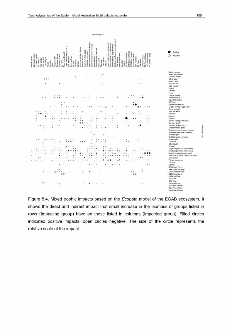
Trophodynamics of the Eastern Great Australian Bight pelagic ecosystem 105
Impacted group
Bal
een
wha
les
Bot
tlnos
ed d
olph
inC
omm
on d
olph
inN
Z fu
r sea
lA
ust f
ur s
eal
Aus
t sea
lion
Littl
e pe
ngui
nP
etre
lsG
anne
tsT
erns
Pel
agic
sha
rks
Dem
ersa
l sha
rks
Ray
s an
d sk
ates
SB
Tun
aO
ther
tuna
s-ki
ngfis
hLa
rge
bent
ho-p
elag
ic p
iscs
Blu
e m
acke
rel
Jack
mac
kere
lR
edba
itA
ncho
vyS
ardi
neIn
shor
e sm
all p
lank
tivor
esS
alm
ons
& ru
ffsM
ediu
m d
emer
sl p
iscs
Sm
all d
emer
sal
pisc
sM
ediu
m d
emer
sal i
nver
t fee
ders
Sm
all d
emer
sal i
nver
t fe
eder
sM
esop
elag
ics
Sm
all d
emer
sal o
mni
vore
Arro
w s
quid
Cal
amar
yO
ther
squ
ids
Oct
opus
Larg
e zo
opla
nkto
n (c
arni
vore
s)S
mal
l zoo
plan
kton
(he
rbiv
ores
)B
enth
ic g
raze
r (m
egab
enth
os)
Det
ritiv
ore
(infa
una
- m
acro
bent
hos)
Filte
r fee
ders
Prim
ary
prod
uctio
nD
isca
rds
Det
ritus
SA
Sar
dine
Fis
hery
SA
MS
-Lin
e Fi
sher
ies
SA
MS
-Net
Fis
herie
sS
BT
-Pur
se S
eine
SB
T-P
ole&
Bai
tS
E T
raw
lG
AB
traw
lD
emer
sal s
hark
SG
-Pra
wn
Fish
ery
GS
V-P
raw
n Fi
sery
WC
-Pra
wn
Fish
ery
Impa
ctin
g gr
oup
Baleen whalesBottlnosed dolphinCommon dolphinNZ fur sealAust fur sealAust sea lionLittle penguinPetrelsGannetsTernsPelagic sharksDemersal sharksRays and skatesSB TunaOther tunas-kingfishLarge bentho-pelagic piscsBlue mackerelJack mackerelRedbaitAnchovySardineInshore small planktivoresSalmons & ruffsMedium demersl piscsSmall demersal piscsMedium demersal invert feedersSmall demersal invert feedersMesopelagicsSmall demersal omnivoreArrow squidCalamaryOther squidsOctopusLarge zooplankton (carnivores)Small zooplankton (herbivores)Benthic grazer (megabenthos)Detritivore (infauna - macrobenthos)Filter feedersPrimary productionDiscardsDetritusSA Sardine FisherySAMS-Line FisheriesSAMS-Net FisheriesSBT-Purse SeineSBT-Pole&BaitSE TrawlGAB trawlDemersal sharkSG-Prawn FisheryGSV-Prawn FiseryWC-Prawn Fishery
Positive
Negative
Figure 5.4. Mixed trophic impacts based on the Ecopath model of the EGAB ecosystem. It
shows the direct and indirect impact that small increase in the biomass of groups listed in
rows (Impacting group) have on those listed in columns (Impacted group). Filled circles
indicated positive impacts, open circles negative. The size of the circle represents the
relative scale of the impact.

Trophodynamics of the Eastern Great Australian Bight pelagic ecosystem 106
Figure 5.5. Estimated proportional breakdown of total annual conumption of sardines and of
all small pelagic fish (sardine, anchovey, blue mackerel, jack mackerel, redbait and inshore
planktivores) by their predators based on the Ecopath model of the EGAB ecosystem. Total
consumption of sardines and of all small pelagic fishes is estimed to be 123,369 t y-1 and
396,129 t y-1, respectively.
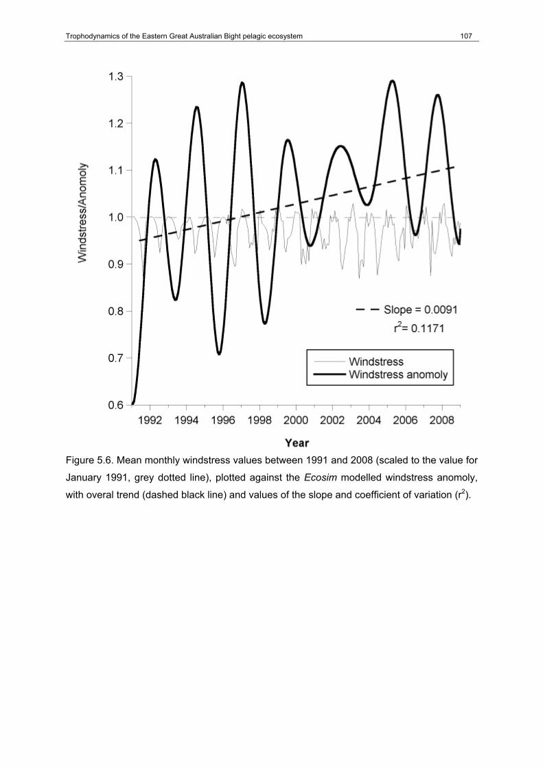
Trophodynamics of the Eastern Great Australian Bight pelagic ecosystem 107
Figure 5.6. Mean monthly windstress values between 1991 and 2008 (scaled to the value for
January 1991, grey dotted line), plotted against the Ecosim modelled windstress anomoly,
with overal trend (dashed black line) and values of the slope and coefficient of variation (r2).

Trophodynamics of the Eastern Great Australian Bight pelagic ecosystem 108
Bio
mas
s (t
km
-2)
Figure 5.7. Time series fits of the EGAB Ecosim model (thin line) to observed biomass
(CPUE) and catch data (dots) for 16 functional groups between 1991 and 2008. The
modelled trend lines (dashed) are provided, together with values of the slope and coefficient
of variation (r2) (see overleaf for remaining plots).

Trophodynamics of the Eastern Great Australian Bight pelagic ecosystem 109
Bio
mas
s (t
km
-2)
Figure 5.7 cont.

Trophodynamics of the Eastern Great Australian Bight pelagic ecosystem 110
A.
B.
Figure 5.8. Estimated changes in the biomass of high trophic level predators based on the
Ecosim EGAB model between 1991 and 2008: A) marine mammals and birds; b) sharks,
rays and skates, tunas and kingfish. Biomass change in NZ and Australian fur seals is forced
in the model as these estimates are based on empircal data for these species in the EGAB
ecosystem.

Trophodynamics of the Eastern Great Australian Bight pelagic ecosystem 111
Figure 5.9. Estimated changes in the biomass of small pelagic fish functional groups, arrow
squid and calarmary based on the Ecosim EGAB model between 1991 and 2008.

Trophodynamics of the Eastern Great Australian Bight pelagic ecosystem 112
A.
B.
C.
D.
Figure 5.10. Ecosystem indicators calculated from the Ecosim EGAB model for the period
1991 to 2008. A. Changes in the landings (catch t y-1) of all fleets (total catch), sardine catch
and other catch; B. Kempton’s Q biomass diversity index; C. Mean trophic level of the catch
and D. Fishing In Balance (FIB) index. Estimated trends are given by dashed lines
(regression), with their coefficient of variation (r2) and level of significance (P).

Trophodynamics of the Eastern Great Australian Bight pelagic ecosystem 113
Figure 5.11. Predicted change in the biomass of functional groups in the Ecosim EGAB
model in 2040 relative to 2008 with sardine biomass reduced to 0.75, 0.50 and 0.25 of 2008
biomass. In this simulation, NZ fur seal and Australian fur seal groups were forced to
increase between 2008 and 2040 (in line with observed increases between 1991 and 2008),
so that population abundances in the EGAB were about 1.5 and 7.0 times present (2008)
levels, respectively (with no change in sardine biomass). Note: the break in the scale of the
x-axis.

Trophodynamics of the Eastern Great Australian Bight pelagic ecosystem 114
Figure 5.12. Predicted change in the biomass of functional groups in the Ecosim EGAB
model in 2040 relative to 2008 with biomass increases of SBT. Biomass increases in SBT
were simulated by reducing effort in the purse seine fishery by adjusting time series values
between 2008 and 2040 under different scenarios of fishing effort (current [2008] levels; 50%
2008 levels; 25% 2008 levels and no fishing effort). In these simulations, NZ fur seal and
Australian fur seal groups were forced to increase between 2008 and 2040 (in line with
observed increases between 1991 and 2008), so that populations abundances in the EGAB
were about 1.5 and 7.0 times present (2008), respectively.

Trophodynamics of the Eastern Great Australian Bight pelagic ecosystem 115
Figure 5.13. Predicted change in the biomass of functional groups in the Ecosim EGAB
model in 2040 relative to 2008 with different scenarios of arrow squid biomass reduction and
with no SBT fishery. Biomass redcution in arrow squid were simulated by adjusting time
series values between 2008 and 2040 under different scenarios of fishing effort (current
[2008] levels; 50% biomass reduction of 2008 levels; 75% biomass reduction of 2008 levels).
In these simulations, NZ fur seal and Australian fur seal groups were forced to increase
between 2008 and 2040 (in line with observed increases between 1991 and 2008), so that
populations abundances in the EGAB were about 1.5 and 7.0 times present (2008),
respectively.

Ecological performance indicators for natural predators of sardines in South Australia 116
6 IDENTIFICATION OF ECOLOGICAL PERFORMANCE
INDICATORS FOR NATURAL PREDATORS OF SARDINE
SARDINOPS SAGAX IN SOUTHERN AUSTRALIA: ASSESSING THE
NEED FOR ECOSYSTEM-BASED MANAGEMENT OF THE SOUTH
AUSTRALIAN SARDINE FISHERY
Page B, Goldsworthy SD, Wiebkin A, Shaughnessy PD, McLeay L, Einoder L, McKenzie J,
Ward T
Introduction
Global fisheries production has averaged about 80-100 million tonnes per year for the past
20 years, which provides about 16% of the animal protein consumed by humans (FAO
1997, FAO 2005). There is concern about the sustainability of this production because many
fisheries are in decline and many are fully-or over-exploited (FAO 2005). Several
international strategies aim to improve fisheries management practices and rebuild fish
stocks, while helping to preserve biodiversity and sustainable stocks (Mora et al. 2009). The
most ambitious of these efforts is the attempt to manage fisheries according to the principles
of ecologically sustainable development, which requires an understanding of impacts on all
species that are affected by fisheries (Fletcher et al. 2002).
Data relating to the population dynamics of exploited species and the ecosystem processes
that influence them are required for models used for fisheries management (Fletcher 2005,
Smith et al. 2007). Because data on ecosystem processes are perceived to be both
expensive to collect and difficult to incorporate into fishery models, management typically
continues with a single-species focus, aimed at ensuring that fish stocks provide the
maximum sustainable yield in the long term (e.g. Smith et al. 2007). This approach is used
effectively in many fisheries, but there is increased recognition at the policy level that
improved knowledge of ecosystem processes will reduce the risk of collapses of fisheries
and populations of predators that use the same stocks (Hutchings 2000, Sainsbury et al.
2000). As a result, there is now considerable interest in the identification, development and
application of ecological performance indicators (EPI) of the state of exploited ecosystems
(Fulton et al. 2005). This has prompted many reviews of the range and suitability of EPIs
that can be used in programs aimed at monitoring human impacts (Kabuta and Laane 2003,
Hiddink and Kaiser 2005, Cury et al. 2005).

Ecological performance indicators for natural predators of sardines in South Australia 117
For EPIs to be of practical use, they must adequately answer the questions raised by their
end users (policy makers, fisheries managers and other stakeholders), by reflecting
changes in the ecosystem that is being exploited (Sainsbury et al. 2000). The concepts that
underlie each EPI must be easy to understand and indicators must be cost effective and
able to be reliably measured (Hiddink and Kaiser 2005). Ecological performance indicators
may also be related to environmental factors, so it is important to understand these
relationships before assuming an EPI reflects human impacts. Most importantly, a significant
relationship between an EPI and an indicator of human impact does not confirm that there is
a relationship between these indicators, rather it highlights them as potential indicators that
require validation (Hiddink and Kaiser 2005).
Because different species of predators vary in their sensitivity to changes in prey availability
over both temporal and spatial scales, the development of EPIs to quantify the impacts of
humans (e.g. fisheries) on natural predators is not straightforward. Ecological performance
indicators are relatively easy to develop and apply if they are based on predator species
with specialised diets, restricted foraging ranges when breeding, variable reproductive
success or high adult survival rates (Furness and Tasker 2000). Ecosystem impacts are
easiest to detect and validate in these predators because they can not compensate for
reductions in prey availability by using different prey (Furness and Tasker 2000).
Relationships between prey availability and EPIs derived from predators are rarely linear,
which increases the data requirements for understanding the nature of a relationship.
Differences in the areas used by predators and a fishery, or where stock assessment for a
fishery is carried out, can also confound apparent impacts of fishing (Hindell et al. 2003).
The identification of EPIs therefore requires that a large number of them are monitored
simultaneously for several species over several years (de la Mare and Constable 2000,
Boyd and Murray 2001). If ecological data from predators show potential as EPIs of fishing
impacts, and the relationship can be validated, they can provide robust, independent and
cost effective measures that can be used to ensure that ecosystem impacts are detected
and minimised (Furness and Tasker 2000, Sainsbury et al. 2000, Kabuta and Laane 2003,
Mori and Butterworth 2006).
Two types of EPI are typically used to assess the impacts of fisheries on predators (modified
from Hindell et al. 2003): 1) Breeding indicators describe the growth and size of offspring,
the survival and reproductive success of individuals, trends in population sizes, abundances,
distribution and emigration/immigration rates, and 2) Foraging indicators describe the diet,
dive effort, at-sea movement patterns and rates of travel. Suites of these EPIs can be used
to examine the effects of changes in the sizes of exploited stocks, prey availability, fishery

Ecological performance indicators for natural predators of sardines in South Australia 118
catches or other human impacts (Furness and Tasker 2000, Sainsbury et al. 2000, Kabuta
and Laane 2003, Mori and Butterworth 2006).
Despite the global interest in the identification and development of EPIs to fulfil the
requirements of international and regional conventions, few fisheries use EPIs to inform
management decisions (FAO 2005, Garcia 2009, Smith and Fulton 2009, Bensley et al.
2010). There are numerous examples where EPIs based on predator biology have been
related to the sizes of commercial fish stocks (see review in Einoder 2009, McLeay et al.
2009b) and fishery catches (Furness 2002, Kabuta and Laane 2003, Hiddink and Kaiser
2005, Fulton et al. 2005), but such EPIs are rarely used by fisheries managers to enhance
their understanding of the state of the ecosystem. The Convention on the Conservation of
Antarctic Marine Living Resources is a notable exception, because it developed and applied
EPIs to assess the impact of the krill (Euphausia superba) fishery on its natural predators in
the Southern Ocean (e.g. Mori and Butterworth 2006). The E. superba fishery is relatively
small by global standards and is considered to be under-exploited (Hewitt et al. 2004).
Ecological performance indicators that describe the breeding and feeding ecology of several
E. superba predators are monitored in several regions and these EPIs are related to
indicators of environmental forcing, E. superba production and fishery catches (Constable
2005, Mori and Butterworth 2006, Heywood et al. 2006). Similarly, EPIs are used to assess
human impacts on the Dutch part of the North Sea to help resource managers evaluate the
impacts of their policies on the health of the ecosystem (Kabuta and Laane 2003). The
impact of the North Sea sandeel (Ammodytes marinus) fishery on the breeding performance
of black-legged kittiwakes (Rissa tridactyla) led to long term fishery closures and ongoing
monitoring of EPIs based on R. tridactyla production, environmental forcing and fishery
impacts (Kabuta and Laane 2003, Frederiksen et al. 2004). The maintenance of these long-
term monitoring datasets provides an opportunity to assess human impacts and
environmental forcing on the health of these exploited ecosystems.
The South Australian sardine fishery has been operating since the early 1990s, with most of
its catch coming from the southern Spencer Gulf. The fishery uses purse seine nets and has
14 licence holders, which currently share the annual allowable catch of 30,000 t (Ward et al.
2008). Australian Government legislation encourages the implementation of ecosystem-
based fisheries management, which requires an understanding of how fisheries compete
with and affect other components of the ecosystem, rather than only quantifying impacts on
target and bycatch species (Fletcher et al. 2002). In 2004, the SA sardine fishery licence
holders, fishery managers and Australian scientists initiated a broad ecological study, which
aimed to assess the impact of the fishery on the natural predators of S. sagax, to determine
whether an ecological allocation of S. sagax was required.

Ecological performance indicators for natural predators of sardines in South Australia 119
In this chapter, we aim to identify EPIs for the key marine predators, which are abundant in
the ecosystem used by the SA sardine fishery. Such EPIs could include measures of
foraging and/or reproductive success, which are likely to be affected by changes in the
distribution and abundance of S. sagax. We also aim to use the results of this study to
provide input for revisions of the management plan of the fishery and establish cost effective
systems for ongoing monitoring and assessment of the ecological effects of the SA sardine
fishery.
Materials and Methods
This study developed and assessed EPIs that described the breeding and feeding ecology
of crested terns (Sterna bergii), New Zealand fur seals (Arctocephalus forsteri), little
penguins (Eudyptula minor), short-tailed shearwaters (Puffinus tenuirostris) and southern
blue-fin tuna (Thunnus maccoyii) (Table 6.1). These key marine predators were chosen for
this study because they are either significant consumers of S. sagax (S. bergii, E. minor,
T. maccoyii, refer Chapter 4) or because trophic models indicated that predators (A. forsteri,
P. tenuirostris, refer Chapter 5) were indirectly affected by changes in the availability of
S. sagax.
Because we were primarily interested in assessing whether the SA sardine fishery was
having a detectable impact on the breeding or feeding ecology of these predators, we
looked for relationships between the EPIs from the marine predators and indicators that
described the activity of the SA sardine fishery and the biomass of the spawning stock. Data
that described trends in the biomass of S. sagax and the annual catch of the fishery were
available for the period between 1995-2007 and 1991-2009, respectively (Table 6.1, Ward
et al. 2008). We initially used data that were recorded in the same year to look for
relationships between each EPI from marine predators and the S. sagax catch and
spawning biomass. To assess whether there was a time lag for these relationships, we
related the S. sagax catch and biomass from the year before the breeding and feeding EPIs
were recorded. We also assessed the relationship between the spawning biomass (but not
catch) from the year after the breeding and feeding EPIs were recorded.
To test the significance of a correlation, data from at least 3 years were required for each
EPI. If the data were available, we used several EPIs to describe similar aspects of the
breeding and feeding ecology of the marine predators. For example, eight EPIs were used
for analyses of the number of E. minor coming ashore at Granite Is, because monthly
averages were available between April-November (Granite Island Penguin Monitoring
Group, Gilbert and Brandle unpublished data). To assess these relationships we used
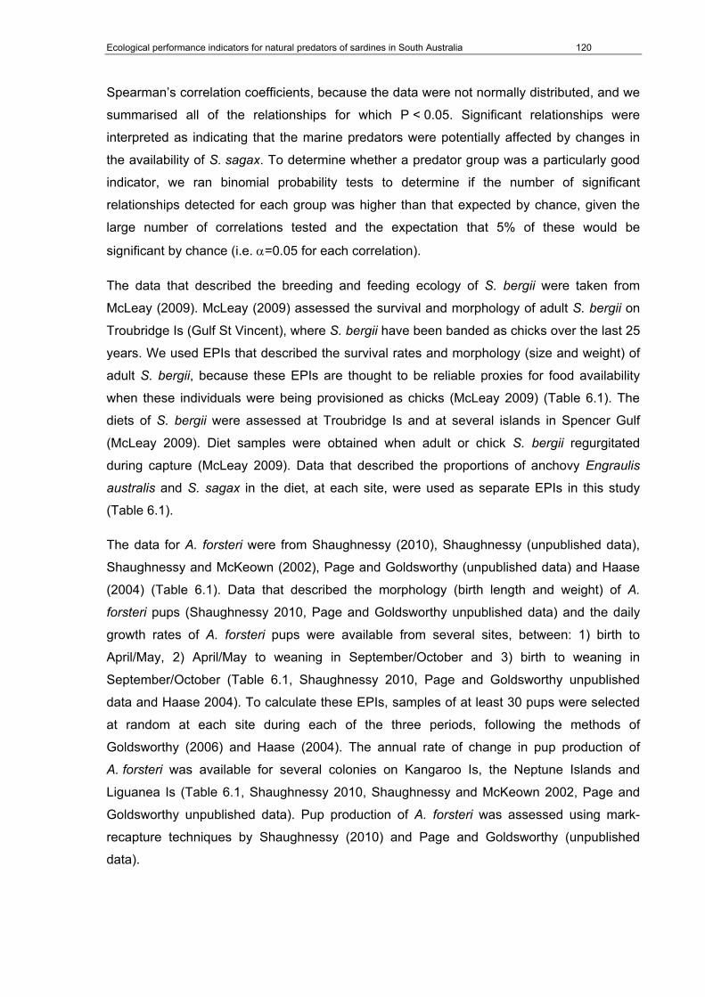
Ecological performance indicators for natural predators of sardines in South Australia 120
Spearman’s correlation coefficients, because the data were not normally distributed, and we
summarised all of the relationships for which P < 0.05. Significant relationships were
interpreted as indicating that the marine predators were potentially affected by changes in
the availability of S. sagax. To determine whether a predator group was a particularly good
indicator, we ran binomial probability tests to determine if the number of significant
relationships detected for each group was higher than that expected by chance, given the
large number of correlations tested and the expectation that 5% of these would be
significant by chance (i.e. =0.05 for each correlation).
The data that described the breeding and feeding ecology of S. bergii were taken from
McLeay (2009). McLeay (2009) assessed the survival and morphology of adult S. bergii on
Troubridge Is (Gulf St Vincent), where S. bergii have been banded as chicks over the last 25
years. We used EPIs that described the survival rates and morphology (size and weight) of
adult S. bergii, because these EPIs are thought to be reliable proxies for food availability
when these individuals were being provisioned as chicks (McLeay 2009) (Table 6.1). The
diets of S. bergii were assessed at Troubridge Is and at several islands in Spencer Gulf
(McLeay 2009). Diet samples were obtained when adult or chick S. bergii regurgitated
during capture (McLeay 2009). Data that described the proportions of anchovy Engraulis
australis and S. sagax in the diet, at each site, were used as separate EPIs in this study
(Table 6.1).
The data for A. forsteri were from Shaughnessy (2010), Shaughnessy (unpublished data),
Shaughnessy and McKeown (2002), Page and Goldsworthy (unpublished data) and Haase
(2004) (Table 6.1). Data that described the morphology (birth length and weight) of A.
forsteri pups (Shaughnessy 2010, Page and Goldsworthy unpublished data) and the daily
growth rates of A. forsteri pups were available from several sites, between: 1) birth to
April/May, 2) April/May to weaning in September/October and 3) birth to weaning in
September/October (Table 6.1, Shaughnessy 2010, Page and Goldsworthy unpublished
data and Haase 2004). To calculate these EPIs, samples of at least 30 pups were selected
at random at each site during each of the three periods, following the methods of
Goldsworthy (2006) and Haase (2004). The annual rate of change in pup production of
A. forsteri was available for several colonies on Kangaroo Is, the Neptune Islands and
Liguanea Is (Table 6.1, Shaughnessy 2010, Shaughnessy and McKeown 2002, Page and
Goldsworthy unpublished data). Pup production of A. forsteri was assessed using mark-
recapture techniques by Shaughnessy (2010) and Page and Goldsworthy (unpublished
data).

Ecological performance indicators for natural predators of sardines in South Australia 121
The diet of T. maccoyii was assessed in the shelf waters off South Australia. Data that
described the proportions of E. australis and S. sagax in the diet of T. maccoyii were the
only EPIs that were analysed for this species (Table 6.1). Stomach samples were obtained
from T. maccoyii caught on trolled lures and the remains of prey were recovered and
identified. Data that described the proportions of anchovy Engraulis australis and S. sagax
in the diet were used as separate EPIs in this study (Table 6.1).
Data that described the breeding and feeding ecology of E. minor were taken from Bool et
al. (2007), Wiebkin (unpublished data) and the Granite Island Penguin Monitoring Group
(Gilbert and Brandle unpublished data). We used EPIs that described the breeding success
of E. minor at several sites, using data that spanned 16 years at Granite Is and 5 years at
Troubridge Is (Table 6.1). Ecological performance indicators of breeding success were
calculated to describe the proportions of E. minor 1) eggs that hatched, 2) eggs that resulted
in fledglings, 3) chicks that resulted in fledglings and 4) the number of chicks fledged per
breeding pair (Table 6.1). Ecological performance indicators that described the morphology
(size and weight) of fledglings were calculated to compare the condition of chicks at the end
of the provisioning period (Table 6.1). The annual rate of change in the population of E.
minor was available at Granite Is between 2000-2009 (Table 6.1, Gilbert and Brandle
unpublished data). The diets of E. minor were assessed at Troubridge Is., Pearson Is and
Reevesby Is (Wiebkin, unpublished data). The stomach contents of E. minor were removed
using the stomach lavaging technique (Wilson 1984) and weighed. The total mass of prey
that each parent returned to its chick was calculated to compare the feeding conditions
around colonies on the day of sampling. Data that described the proportions of E. australis
and S. sagax in the diet at each site and the morphology (size and weight) of these prey
species were used as separate EPIs (Table 6.1). Prey were identified and their weight and
length were estimated by Wiebkin (unpublished data), following the methods of Gales and
Pemberton (1990). The durations of foraging trips by adult E. minor were calculated at
Troubridge Is and Pearson Is from E. minor that were carrying (implanted) tags. Each time
these E. minor came and went from their nests to forage, they passed aerials and a data
logger, which read and stored the identity of the tag and the time (Wiebkin, unpublished
data).
Data that described the breeding and feeding ecology of P. tenuirostris, which were
provisioning chicks at Althorpe Is, were taken from Einoder (2010). We calculated EPIs that
described the breeding success of P. tenuirostris, using data that spanned 3 years (Table
6.1). Ecological performance indicators of breeding success were calculated to describe the
proportions of P. tenuirostris eggs that resulted in fledglings (Table 6.1). The growth rates of
P. tenuirostris chicks were calculated at early and late stages in the provisioning period,

Ecological performance indicators for natural predators of sardines in South Australia 122
based on daily mass measurements (Table 6.1). Growth rates of P. tenuirostris chicks were
modelled and several EPIs that describe the patterns of growth were calculated (Table 6.1).
Short and long foraging trips of P. tenuirostris are thought to be related to local and distant
foraging locations respectively (refer Einoder 2010). To assess local prey availability, we
used EPIs that described the provisioning rate (number of meals per chick) and the number
and proportion of short (1, 2 and 3 d) foraging trips by adults that were provisioning chicks.
The prey of P. tenuirostris were recovered using the stomach lavaging technique (Wilson
1984) and the stomach contents were weighed and identified (Einoder 2010). To compare
the feeding conditions, the total mass of prey that each parent brought back to its chick was
calculated for short (<3 days) and long foraging trips (>3 days) and also for the digested (oil)
and raw components of the stomach contents. Data that described the proportions of E.
australis and S. sagax in the diet were used as separate EPIs (Table 6.1).
Results
In total, 183 EPIs were used to describe the trends in abundance and the breeding and
feeding ecology of S. bergii (44 EPIs), A. forsteri (66 ), E. minor (54), P. tenuirostris (17) and
T. maccoyii (2) (Table 6.1). Annual changes in the EPIs based on predators were compared
with the five indicators that described the S. sagax spawning biomass (3 indicators) and the
catch of the SA sardine fishery (2 indicators), leading to 915 relationships that were tested.
It is not possible to present all of the correlation results, because a total of 915 data sets
were analysed. We summarised the results for EPIs that described similar aspects of the
biology of a predator and the total number of EPIs that were either negatively or positively
related to the catch or biomass of S. sagax (Tables 6.1 and 6.2). For the significant positive
relationships, we present the minimum R value for grouped EPIs and for significant negative
relationships, we present the maximum R value for grouped EPIs.
Of the 220 correlations that related the fishery catch/biomass to the breeding and feeding
ecology of S. bergii, 8 were significant (Tables 6.1 and 6.2). This number of significant
correlations did not differ from the number that would be expected by chance alone (P =
0.225). In Spencer Gulf, the proportion of E. australis in the diet was negatively related to
the S. sagax spawning biomass (R = -1.00) and the S. sagax catch in the previous year (R =
-1.00), but positively related to the S. sagax catch in the same year (R = 1.00). At
Troubridge Is, the proportion of E. australis in the diet showed contrasting relationships with
S. sagax catch (current and previous years), being positively related in the middle of the
breeding season (R = 1.00) and negatively related late in the season (R = -1.00). The bill

Ecological performance indicators for natural predators of sardines in South Australia 123
and head morphology of S. bergii chicks were negatively related to the spawning biomass in
the previous year (R = -0.90).
Of the 330 correlations that related the fishery catch/biomass to the breeding and feeding
ecology of A. forsteri, 15 were significant (Tables 6.1 and 6.2). This number of significant
correlations did not differ from the number that would be expected by chance alone (P =
0.414). The birth morphology of pups on Kangaroo Is and the Neptune Is was negatively
related to the spawning biomass in the current (3 EPIs, R = -1.00) and previous years (1
EPI, R < -0.94) and the catch in the current (6 EPIs, R < -0.47) and previous (2 EPIs, R < -
0.52) years. The growth rate of A. forsteri pups on Kangaroo Is was positively related to the
catch in the previous and current years for 1 EPI (R > 0.97) and negatively related for
another (R = -1.00, Tables 6.1 and 6.2).
In total, 10 correlations were run to compare the diet of T. maccoyii with the fishery
catch/biomass and none of these were significant (Tables 6.1 and 6.2).
Correlations were run to compare the 270 EPIs that described the breeding and feeding
ecology of E. minor with the fishery catch/biomass indicators. Of these, 49 were significant
(Tables 6.1 and 6.2). This number of significant correlations was significantly greater than
the number that would be expected by chance alone (P < 0.001). The morphology of E.
australis in the diet of E. minor was negatively related to the spawning biomass in the
previous year (R = -1.00). The breeding success (eggs to hatch) at Troubridge Is was
positively related to the spawning biomass in the current year (R = 0.99) and the catch in the
previous year (R = 0.88). The morphology of fledglings at Pearson Is (Great Australian
Bight) was positively related to the spawning biomass in the previous year (R = 1.00). The
change in the population size of E. minor at Granite Is was negatively related to the
spawning biomass in the current (R < -0.72), next (R < -0.79) and previous (R < -0.75) years
(each had >7 significant EPIs) and the catch in the current (8 EPIs, R < -0.77) and previous
(6 EPIs, R < -0.67) years. The foraging trip duration of E. minor at Troubridge Is was
positively related to the catch in the previous year (R = 1.00, Tables 6.1 and 6.2).
Of the 85 correlations that related the fishery catch/biomass to the breeding and feeding
ecology of P. tenuirostris, 2 were significant (Tables 6.1 and 6.2). This number of significant
correlations did not differ from the number that would be expected by chance alone (P =
0.196). The daily mass change and growth rates of P. tenuirostris chicks were negatively
related to the catch in the current year (R = -1.00 in both cases, Tables 6.1 and 6.2).

Ecological performance indicators for natural predators of sardines in South Australia 124
Table 6.1. The number of EPIs that were significant for each correlation. EPIs that describe similar relationships are grouped, but each relationship is for
a different test, based on different data sets (e.g. the EPI for crested terns anchovy proportion in diet summarises the relationship between the diet of
crested terns, at several different times of the year versus the fishery parameters).
Predator group and indicator Years No. indicatorsPositive R Negative R Positive R Negative R
SA sardine fisherySpawning biomass 1995-2007 3 - - - -Catch 1991-2009 2 - - - -
Total 5 - - - -Crested tern - Sterna bergiiAnchovy propn in diet (early, mid and late season, GSV) 2003-2007 2 0 0 0 0Anchovy propn in diet (early, mid and late season, GSV) 2004-2007 2 0 0 0 0Anchovy propn in diet (early, mid and late season, GSV) 2005-2007 4 0 0 0 0Anchovy propn in diet (early, mid and late season, Spencer) 2005-2007 5 0 1 0 0Bill and head morphology and body mass, GSV 1985-2000 8 0 0 0 0Sardine propn in diet (early, mid and late season, GSV) 2003-2007 2 0 0 0 0Sardine propn in diet (early, mid and late season, GSV) 2004-2007 2 0 0 0 0Sardine propn in diet (early, mid and late season, GSV) 2005-2007 4 0 0 0 0Sardine propn in diet (early, mid and late season, Spencer) 2005-2007 5 0 0 0 0Survival rate (observed minus modelled), GSV 1985-2000 6 0 0 0 0Survival rate (observed minus modelled), GSV 1985-2002 2 0 0 0 0Survival rate (observed minus modelled), GSV 1986-2003 2 0 0 0 0
Total 44 0 1 0 0New Zealand fur seal - Arctocephalus forsteriBirth morphology, KI 1988-2009 4 0 0 0 0Birth morphology, KI 1989-2007 4 0 0 0 0Birth morphology, KI 2004-2008 2 0 0 0 0Birth morphology, N Neptune 2006-2008 4 0 0 0 0Birth morphology, N&S Neptune 2005-2008 4 0 3 0 0Growth rate cm per day, KI 1995-2006 1 0 0 0 0Growth rate cm per day, KI 1995-2008 1 0 0 0 0Growth rate cm per day, KI 1995-2009 2 0 0 0 0Growth rate cm per day, KI 2001-2007 4 0 0 0 0Growth rate cm per day, KI 2004-2006 2 0 0 0 0Growth rate cm per day, KI 2004-2007 5 0 0 0 0Growth rate cm per day, KI 2004-2010 4 0 0 0 0Growth rate cm per day, KI 2005-2007 8 0 0 0 0Growth rate cm per day, KI 2005-2009 7 0 0 0 0Growth rate cm per day, KI 2005-2010 4 0 0 0 0Growth rate cm per day, N Neptune 2005-2007 2 0 0 0 0Population change KI 1989-2007 2 0 0 0 0Population change KI 1989-2009 1 0 0 0 0Population change N Neptune 2005-2007 1 0 0 0 0Population change N&S Neptune, Liguanea 2005-2007 2 0 0 0 0Population change S Neptune 2005-2007 1 0 0 0 0Population change, Liguanea 2005-2007 1 0 0 0 0
Total 66 0 3 0 0Bluefin tuna - Thunnus maccoyiiAnchovy propn in diet, SA 1999-2006 1 0 0 0 0Sardine propn in diet, SA 1999-2006 1 0 0 0 0
Total 2 0 0 0 0
Spawning biomass (current year) Spawning biomass (next year)Positive R Negative R Positive R Negative R Positive R Negative R
- - - - - -- - - - - -- - - - - -
0 0 0 0 0 00 0 0 0 0 00 0 1 1 1 00 0 1 0 0 10 2 0 0 0 00 0 0 0 0 00 0 0 0 0 00 0 0 0 0 00 0 0 0 0 00 0 0 0 0 00 0 0 0 0 00 0 0 0 0 00 2 2 1 1 1
0 0 0 4 0 20 0 0 0 0 00 1 0 0 0 00 0 0 2 0 00 0 0 0 0 00 0 0 0 0 00 0 0 0 0 00 0 0 0 0 00 0 0 0 0 00 0 0 0 1 00 0 1 0 0 00 0 0 0 0 00 0 0 0 0 10 0 0 0 0 00 0 0 0 0 00 0 0 0 0 00 0 0 0 0 00 0 0 0 0 00 0 0 0 0 00 0 0 0 0 00 0 0 0 0 00 0 0 0 0 00 1 1 6 1 3
0 0 0 0 0 00 0 0 0 0 00 0 0 0 0 0
Catch (prev. year)Spawning biomass (prev. year) Catch (current year)

Ecological performance indicators for natural predators of sardines in South Australia 125
Table 6.1. (cont.)
Predator group and indicator Years No. indicatorsPositive R Negative R Positive R Negative R
Little penguin - Eudyptula minorAnchovy morphology, Pearson 2003-2005 2 0 0 0 0Anchovy morphology, Reevesby 2003-2005 2 0 0 0 0Anchovy morphology, Troubridge 2003-2006 2 0 0 0 0Anchovy propn in diet, Pearson 2003-2005 1 0 0 0 0Anchovy propn in diet, Reevesby 2003-2005 1 0 0 0 0Anchovy propn in diet, Troubridge 2003-2006 1 0 0 0 0Breeding success, chicks to fledge, Granite 1990-2006 1 0 0 0 0Breeding success, eggs to fledge, Granite 1990-2006 1 0 0 0 0Breeding success, eggs to fledge, Granite 1991-2009 1 0 0 0 0Breeding success, eggs to fledge, Troubridge 2004-2009 1 0 0 0 0Breeding success, eggs to fledge, Troubridge 2004-2009 1 0 0 0 0Breeding success, eggs to hatch, Granite 1990-2006 1 0 0 0 0Breeding success, eggs to hatch, Troubridge 2004-2009 1 1 0 0 0Breeding success, eggs to hatch, Troubridge 2004-2009 1 0 0 0 0Breeding success, hatch to fledge, Troubridge 2004-2009 1 0 0 0 0Breeding success, per pair, Troubridge 2004-2009 1 0 0 0 0Breeding success, per pair, Troubridge 2004-2009 1 0 0 0 0Fledging morphology, Pearson 2004-2006 1 0 0 1 0Fledging morphology, Troubridge 2004-2009 3 0 0 0 0Meal mass after trip, Pearson 2003-2005 2 0 0 0 0Meal mass after trip, Reevesby 2003-2005 2 0 0 0 0Meal mass after trip, Troubridge 2003-2006 2 0 0 0 0Population change Granite 2000-2007 8 0 7 0 7Population change Granite 2000-2008 1 0 1 0 0Population change Granite 2001-2008 3 0 3 0 0Population change Granite 2001-2009 1 0 0 0 0Sardine morphology, Reevesby 2003-2005 2 0 0 0 0Sardine morphology, Troubridge 2003-2006 2 0 0 0 0Sardine propn in diet, Pearson 2003-2005 1 0 0 0 0Sardine propn in diet, Reevesby 2003-2005 1 0 0 0 0Sardine propn in diet, Troubridge 2003-2006 1 0 0 0 0Trip duration, Pearson 2004-2006 2 0 0 0 0Trip duration, Troubridge 2004-2006 1 0 0 0 0Trip duration, Troubridge 2004-2009 1 0 0 0 0
Total 54 1 11 1 7Short-tailed shearwater - Puffinus tenuirostrisAnchovy propn in diet, Althorpe 2004-2006 1 0 0 0 0Breeding success, eggs to fledge, Althorpe 2004-2006 1 0 0 0 0Daily mass change, mid and late season, Althorpe 2004-2006 2 0 0 0 0Growth rate, peak mass, r-squared, g/d, Althorpe 2004-2006 3 0 0 0 0Meal mass after trip (short and long), Althorpe 2004-2006 2 0 0 0 0Meal weight (oil + raw, raw only), Althorpe 2003-2006 2 0 0 0 0No. successive short trips, late in season, Althorpe 2004-2006 1 0 0 0 0Propn of 1, 2, 3 d short trips, Althorpe 2004-2006 3 0 0 0 0Provisioning rate, Althorpe 2004-2006 1 0 0 0 0Sardine propn in diet, Althorpe 2004-2006 1 0 0 0 0
Total 17 0 0 0 0Total (all predators, excl. fishery) 183 1 15 1 7
Spawning biomass (current year) Spawning biomass (next year)Positive R Negative R Positive R Negative R Positive R Negative R
0 0 0 0 0 00 1 0 0 0 00 0 0 0 0 00 0 0 0 0 00 0 0 0 0 00 0 0 0 0 00 0 0 0 0 00 0 0 0 0 00 0 0 0 0 00 0 0 0 0 00 0 0 0 0 00 0 0 0 0 00 0 0 0 1 00 0 0 0 0 00 0 0 0 0 00 0 0 0 0 00 0 0 0 0 00 0 0 0 0 00 0 0 0 0 00 0 0 0 0 00 0 0 0 0 00 0 0 0 0 00 7 0 5 0 40 1 0 1 0 10 3 0 1 0 00 1 0 1 0 10 0 0 0 0 00 0 0 0 0 00 0 0 0 0 00 0 0 0 0 00 0 0 0 0 00 0 0 0 0 00 0 0 0 1 00 0 0 0 0 00 13 0 8 2 6
0 0 0 0 0 00 0 0 0 0 00 0 0 1 0 00 0 0 1 0 00 0 0 0 0 00 0 0 0 0 00 0 0 0 0 00 0 0 0 0 00 0 0 0 0 00 0 0 0 0 00 0 0 2 0 00 16 3 17 4 10
Spawning biomass (prev. year) Catch (current year) Catch (prev. year)

Table 6.2. Correlation coefficient for significant correlations (maximum coefficient for negative correlations and minimum for positive correlations). EPI
that describe similar relationships are grouped, but each relationship is for a different test, based on different data sets (e.g. the EPI for crested terns
anchovy proportion in diet summarises the relationship between the diet of crested terns, at several different times of the year versus the fishery
parameters).
Predator group and indicator Positive or negativecorrelation Positive R Negative R Positive R Negative R
Crested tern - Sterna bergiiAnchovy propn in diet (early, mid and late season, GSV) Negative - - - -Anchovy propn in diet (early, mid and late season, GSV) Positive - - - -Anchovy propn in diet (early, mid and late season, Spencer) Negative - -1.00 - -Anchovy propn in diet (early, mid and late season, Spencer) Positive - - - -Bill and head morphology and body mass, GSV Negative - - - -
New Zealand fur seal - Arctocephalus forsteriBirth morphology, KI Negative - - - -Birth morphology, N Neptune Negative - - - -Birth morphology, N&S Neptune Negative - -1.00 - -Growth rate cm per day, KI Negative - - - -Growth rate cm per day, KI Positive - - - -
Little penguin - Eudyptula minorAnchovy morphology, Reevesby Negative - - - -Breeding success, eggs to hatch, Troubridge Positive 0.99 - - -Fledging morphology, Pearson Positive - - 1.00 -Population change Granite Negative - -0.72 - -0.79Trip duration, Troubridge Positive - - - -
Short-tailed shearwater - Puffinus tenuirostrisDaily mass change, mid and late season, Althorpe Negative - - - -Growth rate, peak mass, r-squared, g/d, Althorpe Negative - - - -
Spawning biomass (current year) Spawning biomass (next year)Positive R Negative R Positive R Negative R Positive R Negative R
- - - -1.00 - -- - 1.00 - 1.00 -- - - - - -1.00- - 1.00 - - -- -0.90 - - - -
- -0.94 - -0.47 - -0.52- - - -1.00 - -- - - - - -- - - - - -1.00- - 0.97 - 1.00 -
- -1.00 - - - -- - - - 0.88 -- - - - - -- -0.75 - -0.77 - -0.67- - - - 1.00 -
- - - -1.00 - -- - - -1.00 - -
Catch (prev. year)Spawning biomass (prev. year) Catch (current year)
Ecological performance indicators for natural predators of sardines in South Australia 126

Ecological performance indicators for natural predators of sardines in South Australia 127
Discussion
Our study compared the fishery catch and spawning biomass of S. sagax with EPIs that
described the breeding and feeding ecology of key predators in the same region. The fishery
catch of S. sagax and the spawning biomass were related to many of the EPIs that
described the biology of the predators and as such, these relationships could potentially be
used by fishery managers to monitor changes in the availability of S. sagax and to aid in the
assessment of the need for an ecological allocation of S. sagax. Potential EPIs for the SA
sardine fishery are listed in Table 6.3 and discussed below.
Table 6.3. Potential EPI to implement EBFM in the SA sardine fishery. The EPIs are based
on the breeding and feeding ecology of E. minor, P. tenuirostris, S. bergii and A. forsteri,
and were found to be either negatively related to the fishery catch of S. sagax or positively
related to the spawning biomass of S. sagax. Estimates of the number of days required to
collect the data are provided.
Parameter Location Method to record parameter annuallyE. minorBreeding success Troubridge Is or Lewis Is or
Reevesby IsRecord survival rates of eggs and chicks for 30 burrows (30 days)
P. tenuirostris Growth rate (g/d) of chicks Althorpe Is or North Islet Weigh 50 chicks every 2 days in January
(30 days)
S. bergiiMorphology of fledglings Troubridge Is and Donington
RockMeasure bill length and weigh 200 chicks (16 days)
Survival of fledglings Troubridge Is and Donington Rock
Band 1000 chicks (10 days) and recapture 200 known-age adults (16 days)
A. forsteriBirth mass and length of pups Cape du Coedic, Kangaroo Is or
North Neptune IsMeasure length and weigh 60 pups in late January (4 days)
Growth rate (g/d, cm/d) of pups Cape du Coedic, Kangaroo Is or North Neptune Is
Measure length and weigh 60 pups in January, April and September (12 days)
Practical EPIs need to be sensitive to changes in the ecosystem that is being monitored,
whether they are caused by environmental or anthropogenic impacts, but should not covary
with other factors (Hiddink and Kaiser 2005). We did not assess whether the EPIs were
related to factors such as the catch or biomass of other exploited fish stocks, strength and
timing of seasonal upwelling (e.g. Middleton 2007), abundance or distribution of chlorophyll,
sea surface temperature, or other factors. Covariates reduce the reliability of EPIs and
increase the number and cost of EPIs that need to be monitored. The most practical EPIs

Ecological performance indicators for natural predators of sardines in South Australia 128
based on predator ecology have simple, linear relationships with fishery catches or stock
sizes (reviewed in Einoder 2009). Our analyses were only able to detect linear relationships
and so we would not have detected relationships that were non-linear, which are common in
ecology (e.g. Reid et al. 2005). Nonetheless, the simple, linear EPIs, which we found to be
significantly related to the catch and biomass of S. sagax, serve as a starting point to
determine if ecological allocation in needed for S. sagax.
Because both the SASF catch and spawning biomass have typically increased from one
year to the next, any EPIs that were increasing or decreasing over the same period are likely
to result in a significant relationship. Thus there is a risk that some of the relationships may
be coincidental, because a significant correlation cannot be taken to mean causation. For
example, the population of E. minor at Granite Is (about 250 km from the centre of the
fishery) has been in decline for about 10 years and so the correlations between the indices
that described the size of the penguin population and S. sagax availability were highly
significant (Tables 6.1 and 6.2). The cause of the decline in the penguin population at
Granite Is is not known, but predation by introduced rats (Rattus rattus) and increasing
populations of A. forsteri, and disturbance caused by tourists may be partly responsible
(Bool et al. 2007). The low number of data points available for some of the EPIs (n = 3 for
many relationships, refer Table 6.1), exacerbates this issue, and resulted in many
correlations with R=1 or R=-1. These EPIs all need to be confirmed with additional data
over the coming years.
It is important to highlight that several of the significant relationships between EPIs that
described the breeding and feeding ecology of predators and the catch and biomass of S.
sagax were contrary to our expectations (i.e. positively related to spawning biomass or
negatively related to fishery catch). For example, the morphology of S. bergii was negatively
related to the size of the spawning biomass of S. sagax in the previous year. This finding
does not support those of McLeay et al. (2009b), who showed that S. bergii were smaller
and had lower survival rates if they were from years when S. sagax availability was very low,
which was the case after the two mass mortalities of S. sagax (Ward et al. 2008). Our
analyses may have been too crude to detect these differences, possibly because the
biomass of S. sagax and the breeding performance of S. bergii quickly recovered following
the mass mortalities of S. sagax (Ward et al. 2008, McLeay et al. 2009b). Other unexpected
results included: 1) the negative relationship between the spawning biomass and the
morphology of A. forsteri pups at the Neptune Islands and on Kangaroo Is, and 2) the
negative relationships between the spawning biomass of S. sagax and the EPIs that
described the breeding and feeding ecology of E. minor at Granite Is, as discussed above.
These relationships may also be coincidental or they may reflect the benefits of reduced

Ecological performance indicators for natural predators of sardines in South Australia 129
availability of S. sagax for these predators. Some other significant relationships between
EPIs that described the breeding and feeding ecology of predators and the catch and
biomass of S. sagax were indicative of an abundance of resources in the ecosystem. For
example, the positive relationships between fishery catch and the 1) growth rates of A.
forsteri pups on Kangaroo Is, and 2) E. minor breeding success and trip duration on
Troubridge Is are indicative of abundant prey for these predators and the fishery.
Because our data analyses were conducted to find EPIs that were related to the availability
of S. sagax, it is important to assess how well the suite of indicators met those expectations.
The binomial probability tests indicated that, for S. bergii, A. forsteri, and P. tenuirostris ,
there is a high likelihood that the significant correlations detected occurred by chance alone.
This issue would be resolved with further monitoring of the same relationships.
The population parameters of some predators were related to the availability of S. sagax.
For predator species that were adversely impacted by a reduction in the availability of S.
sagax, we expected to find positive correlations between S. sagax spawning biomass and
EPIs that described the breeding and feeding ecology of predators. We also expected the
EPIs of these predators to be negatively correlated with the catch of the fishery. We did not
have any data to compare the breeding ecology of the juvenile T. maccoyii to the catch or
biomass of S. sagax and none of the EPIs that described the feeding ecology of T. maccoyii
were related to the catch or biomass of S. sagax. For the other predators, the EPIs positively
related to spawning biomass or negatively related to fishery catch included those that
described the morphology and growth rates of A. forsteri pups on Kangaroo Is and Neptune
Is, the breeding success of E. minor at Troubridge Is, the morphology of crested tern
fledglings from Troubridge Is and the growth of P. tenuirostris chicks on Althorpe Is. These
are potentially useful EPIs of the availability of S. sagax and the potential impacts of the S.
sagax fishery in this region. Findings such as these, which summarise relationships between
the breeding and feeding ecology of predators and catch and spawning biomass of a fishery,
are common in the literature, but cases where such findings are used to improve the
fisheries management are rare (e.g. Sainsbury et al. 2000).
The relationship between the spatial distributions of S. sagax and E. australis has received
much research attention, because they are morphologically similar and they appear to
occupy a similar ecological niche. Diet studies conducted on these species in South
Australia indicate that their diets are broadly similar, but there are significant differences in
some of their prey (Daly 2007). In an attempt to understand how S. sagax and E. australis
compete for space, studies have monitored the distribution of eggs, larvae and adult fish
(e.g. Barange and Hampton 1997). In South Australia, S. sagax and E. australis are not

Ecological performance indicators for natural predators of sardines in South Australia 130
spatially segregated and they are thought to compete for spawning habitats, which was
inferred from changes in the relative abundance of the eggs and larvae of the two species
(Ward et al. 2001 a,b). Our results indicate that when the spawning biomass of S. sagax
was relatively high (or the catch of S. sagax was relatively low), the proportion of E. australis
decreased in the diet of S. bergii in Spencer Gulf and at Troubridge Is. In addition, when the
spawning biomass of S. sagax in the previous year increased, the morphology of individual
E. australis was relatively small in E. minor samples from Reevesby Is. These results
support the findings of previous studies, which indicate that adult E. australis are displaced
from near-shore to offshore waters when S. sagax biomass is relatively high (Ward et al.
2001 a,b and Barange and Hampton 1997).
The EPIs that were related to the S. sagax biomass or fishery catch require further
monitoring to confirm that the relationships are real. If validated, the EPIs could be
incorporated as reference points in the management plan for the SA sardine fishery. If a
reference point of an EPI was triggered, it would require investigation to confirm whether this
was caused by a reduction in the availability of S. sagax. If subsequent investigations
indicate that reductions in the biomass of S. sagax were not responsible, the reference
points may need to be adjusted. Such ongoing data collection for the EPIs listed in Table 6.3
could inform and refine the management plan for the SA sardine fishery.
The EBFM for the SA sardine fishery could involve the monitoring of aspects of the breeding
and feeding ecology of S. bergii, A. forsteri, E. minor and P. tenuirostris to reduce the risk of
the fishery having long-term impacts on their populations. Table 6.3 details a potential
monitoring program for the SA sardine fishery, including estimates of the number of days
required to record these data. Monitoring of the EPIs derived from E. minor and
P. tenuirostris would be focused on EPIs that describe breeding success (E. minor) and
growth rates (P. tenuirostris) (Table 6.3). These predators are synchronous breeders,
enabling data to be obtained efficiently at any breeding colony. These EPIs could be
efficiently monitored at sites that are close to the centre of the fishery, such as Lewis Is or
Reevesby Is (E. minor) and Althorpe Is or North Islet (P. tenuirostris) (Table 6.3).
The EPIs derived from A. forsteri, which were related to the availability of S. sagax, were
based on the birth morphology and growth rates of pups (Table 6.3). Pups remain ashore
while lactating females forage at sea. Because lactating females are central place foragers
that use shelf waters between summer and winter (Page et al. 2006, Baylis et al. 2008b,
Page and Goldsworthy unpublished data), the growth rates of pups integrate information
about the availability of prey. Samples of A. forsteri pups can be weighed easily and quickly,
so that rates of growth can be calculated (e.g. Goldsworthy et al. 2006). Colonies of A.

Ecological performance indicators for natural predators of sardines in South Australia 131
forsteri on Kangaroo Is or North Neptune Is are the most appropriate sites for further
monitoring because: 1) there are data sets that span more than 20 years for these EPIs, 2)
the colonies are easy to access, and 3) females from these colonies use waters immediately
to the south of Spencer Gulf, where the fishery is centred (Baylis et al. 2008 a,b, Page and
Goldsworthy unpublished data) (Table 6.3).
Based on our understanding of the trophic (Chapter 3 and 5) and spatial (Chapter 4)
dynamics of S. bergii, A. forsteri, E. minor and P. tenuirostris, the most likely species that
would be affected by a change in the availability of S. sagax is S. bergii. As discussed in
chapter 3, S. sagax are a very small part of the diet of A. forsteri, E. minor and P. tenuirostris
and so even if future research showed that EPIs based on these predators were significantly
related to S. sagax availability, the relationship is not likely to be direct. The results of the
trophodynamic model support these conclusions, because S. bergii demonstrated the
greatest sensitivity to reduction in S. sagax biomass (Chapter 5). Given these findings, the
most appropriate form of EBFM for the SA sardine fishery would include the monitoring the
EPIs based on S. bergii, as outlined in Table 6.3.
Because the morphology and survival of S. bergii at Troubridge Is have been shown to be
related to the availability of S. sagax (McLeay et al. 2009b), this species requires ongoing
monitoring at Troubridge Is (Table 6.3). Colonies of S. bergii are readily accessible and at
breeding colonies, large proportions of the adult birds can be captured, identified and/or
aged (from bands applied when they were chicks), measured and released in a relatively
brief period, making this a cost-effective species for monitoring. Efforts should also be made
to monitor the morphology and survival of S. bergii at a colony in Spencer Gulf (e.g.
Donington Rock), near the centre of the SA sardine fishery, because the effects of localised
depletions of S. sagax are likely to be most apparent there (Table 6.3).
This study focussed on EPIs that described the relationships between the biology of
predators and the availability of S. sagax. Goldsworthy et al. (Chapter 5) used an alternative
approach – trophodynamic modelling – to address the same question from a broader
perspective. Their model simulated the dynamics of the ecosystem by incorporating all
available data on the ecosystem, including: 1) the diets and demographics of the predators
in the region, 2) annual changes in environmental features such as upwelling, 3) the annual
catches of the fisheries in the region. In addition to confirming the potential for S. bergii as
an EPI, Goldsworthy et al. (Chapter 5) indicated that the current level of the SA sardine
fishery was unlikely to be adversely affecting the ecosystem. The ability to evaluate the role
of multiple components of the ecosystem, including the impacts of different fisheries,
highlights the benefit of using this broad-based approach to monitor changes in key EPIs of

Ecological performance indicators for natural predators of sardines in South Australia 132
the ecosystem. Periodic updates, for example every five years, of the trophodynamic model,
including further data inputs (based on the biology of predators, catches of fisheries and
environmental features) and improvements to the design of the model, together with the
annual monitoring of the EPIs discussed in this chapter, will ensure that significant progress
is made toward the EBFM of the SA sardine fishery.
Monitoring of this ecosystem in such a manner would provide fishery managers with data
that may help them alleviate the impacts of localised depletions caused by the fishery, for
example through quota and/or spatial management of fishing activity. This approach is
employed by fishery managers of: 1) the sandeel (A. hexapterus) fishery in the North Sea
(Kabuta and Laane 2003), and 2) E. superba fishery in the Antarctic to minimise the impact
on the natural predators of E. superba, as part of CCAMLR (Convention on the
Conservation of Antarctic Marine Living Resources). Annual monitoring of EPIs for S. bergii
and periodic updates of trophodynamic models will also ensure that monitoring is focussed
on cost effective methods, which provide fishery managers with a means to assess the
effects of their management strategies.

Benefits and adoption 133
7 BENEFITS AND ADOPTION
Industry/community sectors benefiting from research
The SASF has a high public profile and is subject to considerable external scrutiny
because it is the largest single-species fishery in Australia and targets a forage species
that is widely acknowledged to play a critical role in converting planktonic biomass into a
form that is accessible to large predatory species, which have high conservation value.
The main findings of this study, i.e. that current harvest levels in the SASF are not
adversely affecting ecosystem function or the populations of key predators, are critically
important to licence-holders in the SASF and the tuna aquaculture industry of southern
Spencer Gulf, which utilises much of the catch, because they help to ensure ongoing
access to this valuable resource.
The benefits to conservation agencies and other fisheries are also significant because this
project delivers the type of ecosystem-based assessment of the potential impacts of
fishing that is often requested or recommended, but rarely undertaken at the scale of this
project.
The findings in this report provide conservationists and the general public with evidence
that fisheries management of the SASF is functioning effectively, despite the gloomy
global prognosis for many fisheries.
The State and Commonwealth agencies responsible for the management of Australia’s
living marine resources also benefit from the evidence that shows not only is the SASF
being managed according to the principle of ESD, but that the valuable Flinders Current
Ecosystem off southern Australia is functioning well and remains productive. This study
also benefits these agencies by providing, arguably for the first time, the data and tools
required to objectively assess the potential benefits of establishing ecological performance
indicators and reference points for a pelagic fishery in Australian waters.
One example highlights the international recognition for ecological sustainability that this
and previous studies have delivered to the SASF. In October 2009, the Marine
Stewardship Council used the SASF as a case study to assist the development of a new
Fishery Assessment Methodology for the management of fisheries for low trophic level
species.

Benefits and adoption 134
This project provided substantial opportunities for post graduate research in South
Australia. This project collated data from 10 projects (6 PhD and 4 honours), which were
entirely or partly funded by this FRDC project. The names of the students and their
projects are listed below.
PhD projects
Dr Alastair Baylis – The University of Adelaide. Project title: Seasonal and colony
differences in the foraging ecology of New Zealand fur seals.
Dr Luke Einoder – The University of Adelaide. Project title: Feeding and breeding ecology
of the short-tailed shearwater in South Australia.
Dr Lachlan McLeay – The University of Adelaide. Project title: The life history characters,
reproductive constraints and foraging strategies of the crested tern.
Dr Annelise Wiebkin – The University of Adelaide. Project title: The feeding and breeding
ecology of little penguins in South Australia.
Dr Kristian Peters – The University of Adelaide. Project title: Molecular and morphological
analyses of Australian sea lion diet.
Mr Paul Rogers – Flinders University. Project title: Movement, diet and population
structure of pelagic shark populations in southern Australia.
Honours projects
Dr Robin Caines – The University of South Australia. Project title: Trophic Guild-Structures
in Pelagic Fish Communities in the Eastern Great Australian Bight Ecosystem.
Ms Natalie Bool – The University of Adelaide. Project title: What is causing the decline of
little penguins (Eudyptula minor) on Granite Island, South Australia?
Ms Michelle Roberts – The University of Adelaide. Project title: Assessment of
morphological and molecular diet analysis techniques: application of a combined approach
to resolve the diet of arrow squid, Nototodarus gouldi in the eastern Great Australian Bight.
Ms Kerryn Daly – The University of Adelaide. Project title: The diet and guild structure of
the small pelagic fish community in the eastern Great Australian Bight, South Australia.
Benefits and adoption 135
Adoption of the research by identified beneficiaries
The results of this project will be used to assess the potential benefits of establishing
ecological performance indicators and reference points in the management plan for the
SASF. The ecosystem model that was developed will be available for ongoing analyses,
including regular generation (e.g. every five years) of indicators of ecosystem health
(Kempton’s Q biodiversity index, Fishing in Balance index). Similarly, dietary and foraging
data collected will provide a basis for developing time series of potential ecological
performance indicators such as breeding success of crested terns. The adoption of these
findings will help to ensure that Australia’s largest fishery continues to meet, exceed and
set internationally-recognised standards for world’s best practice in the ecosystem-based
management of fisheries for low trophic level species.
Summary of project extension to beneficiaries
The research and management working groups for the SASF have regularly been updated
on the progress of the project. Presentations of preliminary results have also been made
to the Resource Assessment Group of the Commonwealth Small Pelagic Fishery. Final
results will be presented to both of these groups early in 2011. Preliminary results have
also been presented to the Marine Stewardship Council (Washington, DC, October 2009)
and Sardine Tri-national Forum (Victoria Canada November 2010).
How benefits and beneficiaries compare to those identified in the original
application
The benefits and beneficiaries of the project are consistent with those identified in the
original application. The proposal indicated that the results of this study would assist the
SASF, PIRSA Fisheries and SARDI Aquatic Sciences to revise the management plan for
the SASF and establish cost-effective systems for ongoing monitoring and assessment of
the ecological effects of the SASF. This will be done during the revision of the
management plan for the SASF, which is scheduled to be completed by 30 June 2013.
Potential ecological performance indicators identified in this project include the model-
based indices (e.g. Kempton’s Q biodiversity index, Fishing in Balance index) and foraging
patterns and reproductive success of the crested tern.

Further development 136
8 FURTHER DEVELOPMENT
The current fishery management strategy appears to be sufficiently conservative to ensure
that the fishery is managed according to the principles of ecological sustainable
development (ESD). However, the extent to which this positive assessment reflects
management of the sardine fishery is uncertain, given that much of the positive changes
estimated by the model reflect other changes in the ecosystem, including reductions in
fishing effort and mortality in some fleets (SA marine scalefish net and Commonwealth
demersal gillnet shark fishery), and a positive trend in primary production over the study
period. How the current or alternate management strategies of the sardine fishery would
perform under alternate oceanographic conditions (such as more variable upwelling),
and/or in response to management changes in other fisheries in the EGAB region, may
warrant consideration.
The trophodynamic models developed in Chapter 5 provide a basis for examining
additional management measures and ecological questions. The performance indicators
produced by the Ecosim model also provide a means to assess the potential impacts of
the SASF relative to those of other fisheries and environmental change. The ability to
resolve and attribute potential impacts from multiple fishing fleets and environmental
changes provided by these models will be critical for the development of ecological
performance indicators for assessing ESD targets.
The results of this study indicate that one potential EPI warrants further investigation.
McLeay et al (2009) showed that large reductions sardine biomass may affect the foraging
patterns and reproductive success of the crested tern. This potential for reproductive
parameters for this species to be incorporated into the management plan for the SASF
warrants further investigation.

Planned outcomes 137
9 PLANNED OUTCOMES
Social, economic and ecological advantages
The South Australian community, tuna farmers and participants in the SASF have benefited
from ongoing access to local sardines and a reduced need to import baitfish into Australia.
The project is helping to maintain the status of the SASF as one of Australia’s best managed
fisheries, and Australia’s position as a world leader in EBFM.
Ecologically sustainable management of the SA sardine fishery
The ecosystem and trophodynamic model developed in this study provides an intellectual
framework and practical tool to underpin EBFM of the Flinders Current ecosystem. These
models, which take into account the spatial and temporal variability of the eastern GAB
ecosystem, will allow fishery managers to investigate the potential consequences of
increasing the SASF quote, on ecosystem function and the populations of several protected
species. This study also identified that there would be benefits in establishing a monitoring
program to assess the potential for using reproductive parameters of the crested tern
S. bergii as ecological performance indicators in the SASF.
Conservation of seabird and marine mammal populations
Information on the feeding grounds of key predators that this report provided has facilitated
a better understanding of the environmental mechanisms that underpin the ecology of this
region. The SA Department of Environment and Natural Resources will use this and other
information collected in this study to manage marine mammal, penguin and other seabird
populations that breed on islands in the GAB ecosystem.

Conclusions 138
10 CONCLUSIONS
DIETS OF MARINE PREDATORS IN SOUTH AUSTRALIA
This study indicated that, based on their diets, the 37 predator groups considered could be
categorised into 8 feeding guilds. The SA sardine fishery (based on its catch) was included
in a guild with 10 predator groups (common thresher shark, west Australian salmon,
common dolphin, little penguin, bonito, Australian gannet, snook, crested tern, southern
bluefin tuna and barracouta), which were considered as the species that are most likely to
be directly impacted by competition with the SASF. The importance of sardines to the
predators in this guild and to some of the other predators in different guilds (e.g. bronze
whaler sharks, Gould’s squid and kingfish) highlights the benefits of ongoing monitoring of
ecosystem processes in the region where the SA sardine fishery is located.
SPATIAL DISTRIBUTION OF CONSUMPTION EFFORT OF KEY APEX PREDATORS
AND THEIR OVERLAP WITH THE SARDINE FISHERY
Most of the consumption by the five key land-breeding apex predators studied consisted of
fish (53%), squid (39%) and crustaceans (7%). Small pelagic fish accounted for 28% of the
total consumption and 52% of the total fish consumed in the EGAB (Table 4.3). Overall,
sardines only made up about 1% of the total prey biomass consumed by the five apex
predators, and only 2% of the total fish biomass consumed (Table 4.3). The total estimated
consumption of sardines by these predators (753 t/y) is very small (3%) relative to the
current annual TACC (30,000 t) of the SA sardine fishery. As such, the catch of sardines by
the fishery exceeds the consumption by the five apex predators wherever fishing effort
occurs. Outside of the area used by the fishery there are large areas where consumption of
sardines by the five apex predators exceeds that of the fishery (Figure 4.2. F).
Based on the analysis of the spatial distribution of prey consumption by five key land-
breeding apex predators in the EGAB ecosystem, crested terns were the only species
identified for which sardine consumption represented a significant component of total prey
consumed (22.7%), and this consumption overlapped with the core region used by the
SASF in southern Spencer Gulf and Investigator Strait (Figure 4.1. and 4.2.). Therefore, of
all the species investigated, crested terns are most likely to provide potential ecological
performance indices for the SA sardine fishery, because spatial and consumption analyses

Conclusions 139
suggest they may integrate information on the availability of sardines into their foraging,
reproductive and population ecology.
TROPHODYNAMICS OF THE EASTERN GREAT AUSTRALIAN BIGHT PELAGIC
ECOSYSTEM
The growth of the sardine fishery in the EGAB region since its establishment in 1991 has
been rapid, and its catch now exceeds that of all other fisheries by a factor of three. Despite
this, sensitivity analyses based on mixed trophic impacts detected negligible impacts on
other predators. The ecosystem performance indicators produced by the Ecosim model
provide a means to assess the potential impacts of the sardine fishery relative to those from
other fisheries and environmental change. These model-based indicators could be
generated every 5 years to monitor the health of the ecosystem. The trophodynamic model
indicated that crested terns demonstrated the greatest sensitivity to reduction in sardine
biomass, supporting the findings of Chapters 3 and 4 and highlighting their potential to be
used as EPIs for the SASF.
The use of trophodynamic models as a tool to provide context to the potential impacts and
management strategies of a single fishery relative to the temporal changes of a complex
dynamic ecosystem subject to dynamic impacts from multiple fishing fleets and climate
change, is highlighted by this study. The model provides a basis from which future
improvements in model design and data inputs will enable more complex management and
ecological questions to be examined.
ECOLOGICAL PERFORMANCE INDICATORS (EPIS) FOR NATURAL PREDATORS OF
SARDINE IN SOUTHERN AUSTRALIA
Most of the datasets that described the ecological performance of predators were collected
over the 3 or 4 year period of the study, which is a relatively brief period to assess the state
of such a productive and dynamic ecosystem. Thus the relationships that we presented may
not be robust, and it is likely that some of the significant relationships are non-significant and
vice versa. The results indicated that the morphology and growth rates of New Zealand fur
seal pups on Kangaroo Is, the breeding success of little penguins at Troubridge Is, the
morphology of crested tern fledglings from Troubridge Is and the growth of short-tailed
shearwater chicks on Althorpe Is were negatively correlated with the annual catch of the
SASF. However, sardines are a very small part of the diet of New Zealand fur seals, little

Conclusions 140
penguins and short-tailed shearwaters and these predators do not overlap significantly with
the area that is typically used by the fishery (chapter 4).
Like previous chapters, the results of this chapter indicated that the species most likely to be
impacted by reductions in the availability of sardines is crested terns.
The most appropriate form of EBFM for the SA sardine fishery would include monitoring of
the morphology and survival of crested terns together with periodic updates of the EPIs that
are derived from the trophodynamic model. Efforts should be made to monitor the EPIs for
crested terns at colonies in Spencer Gulf (e.g. Donington Rock) and at Troubridge Is. To
provide a broader perspective of the potential impact of the SA sardine fishery in the
ecosystem, the trophodynamic model should be updated every five years, to incorporate all
of the available data (based on the biology of predators, catches of fisheries and
environmental features) and improvements to the design of the model.
Relationships between the breeding and feeding ecology of predators and catch and
spawning biomass of a fishery are commonly reported in the literature, but cases where
such findings are used to improve the management of a fishery are rare. Validation of the
relationships between EPIs based on crested terns versus sardine availability will ensure
that monitoring is focussed on data that can be collected efficiently and that can be used by
fishery managers to assess the effects of their management strategies. This approach will
ensure that the SA sardine fishery remains a world leader in the implementation of EBFM
.

References 141
11 REFERENCES
Ainsworth CH, Pitcher TJ (2006) Modifying Kempton’s species diversity index for use with ecosystem simulation models. Ecological Indicators 6:623-630
Andersson M. 1994. Sexual selection. Princeton University Press, USA Aqorau, T., Ed. (2003). Obligations to protect marine ecosystems under international
conventions and other legal instruments. Responsible fisheries in the marine ecosystem. Rome, Italy, Food and Agriculture Organization of the United Nations.
Arnould JPY, Warneke RM (2002) Growth and condition in Australian fur seals (Arctocephalus pusillus doriferus) (Carnivora: Pinnipedia). Australian Journal of Zoology 50:53-66
Ashmole NP. (1968) Body size, prey size and ecological segregation in 5 sympatric tropical terns (Aves: Laridae). Systematic Zoology 17:292–304
Barange M., and Hampton I. (1997) Spatial structure of co-occurring anchovy and sardine populations from acoustic data: implications for survey design. Fisheries Oceanography, 6: 94-108.
Barlow J, Boveng P (1991) Modelling age-specific mortality for marine mammals populations. Marine Mammal Science 7:84-119
Barlow J, Kahru M, Mitchell BG (2008) Cetacean biomass, prey consumption, and primary production requirments in te California Current ecosystem. Marine Ecology Progress Series 371:285-295
Barlow K, Boyd I, Croxall J, Reid K, Staniland I and Brierley A. (2002) Are penguins and seals in competition for Antarctic krill at South Georgia? Marine Biology, 140: 205-213
Basson M, Kolody D, Polacheck T, Preece A and Hartog J (2004) Assessment and projections of SBT stock assessment and summary of agreed stock status reference points. CCSBT-ESC/0904/23.
Baum, J. K., R. A. Myers, D. G. Kehler, B. Worm, S. J. Harley and P. A. Doherty (2003). Collapse and conservation of shark populations in the Northwest Pacific. Science 299, 389-392.
Baylis AMM, Page B, Goldsworthy SD (2008a) Colony-specific foraging areas of lactating New Zealand fur seals. Marine Ecology-Progress Series 361:279-290
Baylis AMM, Page B, Goldsworthy SD (2008b) Effect of seasonal changes in upwelling activity on the foraging locations of a wide-ranging central-place forager, the New Zealand fur seal. Canadian Journal of Zoology-Revue Canadienne De Zoologie 86:774-789
Beals EW. (1984) Bray Curtis ordination: an effective strategy for analysis of multivariate ecological data. Adv Ecol Res 14:1–55
Beamish, R. J. D., Noakes, J., McFarlane, G. A., Klyashtorin, L., Ivanov, V. V., Kurashov, V. (1999) The regime concept and natural trends in the production of Pacific salmon. Canadian Journal of Fisheries and Aquatic Science: 56: 516-526
Bensley N., Stobutzki I., and Begg G. (2010) An integrated approach to wildlife bycatch: addressing key issues to progress the implementation of national plans of action, BRS report prepared for the Department of Agriculture, Fisheries and Forestry, Canberra, July.
Bethge P, Nicol S, Culik BM, Wilson RP (1997) Diving behaviour and energetics in breeding little penguins (Eudyptula minor). Journal of Zoology, London 242:483-502
Bool N.M., Page B., Goldsworthy S.D. (2007) What is causing the decline of little penguins (Eudyptula minor) on Granite island, South Australia. Report to the

References 142
South Australian Department for Environment and Heritage, Wildlife Conservation Fund and the Nature Foundation SA, July 2007. SARDI Publication Number: F2007/000288-1. SARDI Research Report Series No: 217, 55pp.
Boyd I. L., and Murray A. W. A. (2001) Monitoring a marine ecosystem using responses of upper trophic level predators. Journal of Animal Ecology. 70:747-760.
Braley M, Goldsworthy SD, Page B, Steer M, Austin JJ (2010) Assessing morphological and DNA-based diet analysis techniques in a generalist predator, the arrow squid Nototodarus gouldi. Molecular Ecology Resources 10:466-474
Branch TA, Stafford KM, Palacios DM, Allison C, Bannister JL, Burton CLK, Cabrera E, Carlson CA, Vernazzani BG, Gill PC, Hucke-Gaete R, Jenner KCS, Jenner MNM, Matsuoka K, Mikhalev YA, Miyashita T, Morrice MG, Nishiwaki S, Sturrock VJ, Tormosov D, Anderson RC, Baker AN, Best PB, Borsa P, Brownell RL, Childerhouse S, Findlay KP, Gerrodette T, Ilangakoon AD, Joergensen M, Kahn B, Ljungblad DK, Maughan B, McCauley RD, McKay S, Norris TF, Whale O, Rankin S, Samaran F, Thiele D, Van Waerebeek K, Warneke RM, Dolphin Res G (2007) Past and present distribution, densities and movements of blue whales Balaenoptera musculus in the Southern Hemisphere and northern Indian Ocean. Mammal Rev 37:116-175
Brooke, M. (2004). Albatrosses And Petrels Across The World. Oxford University Press, Oxford, UK
Brown CJ, Fulton EA, Hobday AJ, Matear RJ, Possingham HP, Bulman C, Christensen V, Forrest RE, Gehrke PC, Gribble NA, Griffiths SP, Lozano-Montes H, Martin JM, Metcalf S, Okey TA, Watson R, Richardson AJ (2010) Effects of climate-driven primary production change on marine food webs: implications for fisheries and conservation. Global Change Biology 16:1194-1212
Bruce, B. D. and D. A. Short (1990). Observations on the distribution of larval fish in relation to a frontal system at the mouth of Spencer Gulf, South Australia. Bureau of Rural Resources Proceedings 15, 124-137.
Bruce, B. D., Stevens, J. D. and Malcolm, H. (2006). Movements and swimming behaviour of white sharks (Carcharodon carcharias) in Australian waters. Marine Biology: 150: 161–172.
Bulman C, Althaus F, He X, Bax NJ, Williams A (2001) Diets and trophic guilds of demersal fishes of the south-eastern Australian shelf. Marine and Freshwater Research 52:537-548
Bulman C, Condie S, Furlani D, Cahill M, Klaer N, Goldsworthy S, Knuckey I (2006) Trophic dynamics of the eastern shelf and slope of the South East Fishery: impacts of an on the fishery. Final Report to the Fisheries Research and Development Corporation (FRDC 2002/028). CSIRO Marine and Atmospheric Research, Hobart, Tasmania. In:
Bulman CM, Condie SA, Neira FJ, Goldsworthy SD, Fulton EA (2010) The trophodynamics of small pelagic fishes in the southern Australian ecosystems and the implications for ecosystem modelling of southern temperate fisheries. Final Report to the Fisheries Research and Development Corporation (FRDC 2008/023). CSIRO Marine and Atmospheric Research, Hobart, Tasmania. In:
Bunce A (2001) Prey consumption of Australasian gannets. (Morus serrator) breeding in Port Philip Bay, southeast. Australia, and potential overlap with commercial fisheries. ICES Journal of Marine Science, 58: 904–915
Bundy A (2001) Fishing on ecosystems: the interplay of fishing and predation in NewFoundland-Labrador. Canadian Journal of Fisheries and Aquatic Sciences 58:1153–1167
Caines R. (2005) Trophic guild-structure in pelagic fish communities in the eastern
References 143
Great Australian Bight Ecosystem. Honours thesis, University of South Australia.
Camphuysen, C. J., B. E. Scott and S. Wanless, Eds. (2006). Distribution and foraging interactions of seabirds and marine mammals in the North Sea: multispecies foraging assemblages and habitat-specific feeding strategies. Top predators in marine ecosystems: Their role in monitoring and management Cambridge, Cambridge University Press.
Chiaradia A, Costalunga A, Kerry K (2003) The diet of Little Penguins (Eudyptula minor) at Phillip Island, Victoria, in the absence of a major prey - Pilchard (Sardinops sagax). Emu 103:43-48
Chiaradia A, Dann P, Jessop R, Collins P (2002) The diet of Crested Tern (Sterna bergii) chicks on Phillip Island, Victoria, Australia. Emu 102:367-371
Christensen V (2000) Indicators for marine ecosystems affected by fisheries. Marine and Freshwater Research 51:447-450
Christensen V, Pauly D (1992) Ecopath II - a software for balancing steady-state ecosystem models and calculating network characterisitics. Ecological Modelling 61:169-185
Christensen V, Walters CJ (2004) Ecopath with Ecosim: methods, capabilities and limitations. Ecological Modelling 172:109-139
Christensen V, Walters CJ, Pauly D, Forrest R (2008) Ecopath with Ecosim version 6 User Guide, November 2008. Lenfest Ocean Futures Project 2008. In:
Colabuono FI and Vooren CM (2007) Marine Ornithology The diet of the Black-browed Albatross Thalassarche melanophrys, Atlantic Yellow -nosed Albatross T. chlororhynchos, White-chinned Procellaria aequinoctialis and Spectacled P. conspicillata petrels off southern Brazil. Marine Ornithology 35: 9-20.35: 9–20
Coll M, Santojanni A, Palomera I, Arneri E (2009) Food-web changes in the Adriatic Sea over the last three decades. Marine Ecology Progress Series 318:17-37
Collette BB and Nauen CE. (1983) FAO species catalogue. Vol.2. Scombrids of the world. An annotated and illustrated catalogue of tunas, mackerels, bonitos and related species known to date. United Nations Development Programme Food and Agriculture Organization of the United Nations, Rome 1983. 137 p
Constable A.J. (2005) A possible framework in which to consider plausible models of the Antarctic marine ecosystem for evaluating krill management procedures. CCAMLR Science, 12: 99–117.
Constable, A. J. and S. Nicol (2002). Defining smaller-scale management units to further develop the ecosystem approach in managing large-scale pelagic krill fisheries in Antarctica. CCAMLR Science 9, 117-131.
Constable, A. J., W. K. de la Mare, D. J. Agnew, I. Everson and D. Miller (2000). Managing fisheries to conserve the Antarctic marine ecosystem: practical implementation of the Convention on the Conservation of Antarctic Marine Living Resources (CCAMLR). ICES Journal of Marine Science 57, 778-791.
Copley, P.B. (1996) The status of seabirds in South Australia. In: Ross, G.J.B., K. Weaver & J.C. Grieg, eds. The Status of Australia's Seabirds: Proceedings of the National Seabird Workshop. Canberra, 1-2 November 1993. Page(s) 139--180. Biodiversity Group, Environment Australia, Canberra.
Cornejo-Donoso J, Antezana T (2008) Preliminary trophic model of the Antarctic Peninsula Ecosystem (Sub-area CCAMLR 48.1). Ecological Modelling 218:1-17
Costa DP, Dann P, Disher W (1986) Energy requirements of free ranging little penguin, Eudyptula minor. Comparative Biochemistry and Physiology 85A:135-138
Costa DP, Gales NJ (2000) Foraging energetics and diving behaviour of lactating New Zealand sea lions, Phocarctos hookeri. Journal of Experimental Biology 203:3655-3665
Costa DP, Gentry RL (1986) Reproductive energetics of the northern fur seal. In:

References 144
Gentry RL, Kooyman GL (eds) Fur Seals: Maternal Strategies on Land and at Sea. Princeton University Press, Princeton, New Jersey
Crawford RJM, Sabarros PS, Fairweather T, Underhill LG and Wolfaardt AC (2008) Implications for seabirds off South Africa of a long-term change in the distribution of sardine. African Journal of Marine Science 30(1): 177–184
Currie DR, Dixson CD, Roberts SD, Hooper GE, Sorokin SJ, Ward TM (2009) Fishery-independent by-catch survey to inform risk assessment of the Spencer Gulf Prawn Trawl Fishery. Report to PIRSA Fisheries. South Australian Research and Development Institue (Aquatic Sciences), Adelaide. SARDI Publication No. F2009/000369-1. SARDI Research Report Series No. 390. In:
Currie DR, Sorokin SJ (2010) A preliminary evaluation of the distribution and trophodynamics of demersal fish from Spencer Gulf. Report to the South Australian Department for the Environment and Heritage. South Australian Research and Development Institue (Aquatic Sciences), Adelaide. SARDI Publication No. F2010/000088-1. SARDI Research Report Series No. 424. In:
Cury P, Bakun A, Crawford RJM, Jarre A, Quinones RA, Shannon LJ, Verheye HM (2000) Small pelagics in upwelling systems: patterns of interaction and structural changes in "wasp-waist" ecosystems. ICES Journal of Marine Science 57:603-618
Cury P.M., Shannon L.J., Roux J.P., Daskalov G.M., Jarre A., Moloney C.L., Pauly R. (2005) Trophodynamic indicators for an ecosystem approach to fisheries. ICES Journal of Marine Science. 62: 430-442.
Daly K. (2007) The diet and guild structure of the small pelagic fish community in the eastern Great Australian Bight, South Australia. Honours thesis, University of Adelaide.
Dann P, Carron M, Chambers B, Chambers L, Dornom T, McLaughlin A, Sharp B, Talmage ME, Thoday R, Unthank S (2005) Longevity in Little Penguins Eudyptula minor. Marine Ornithology 33:71-72
Dann P, Cullen JM (1990) Survival, Patterns of Reproduction and Lifetime Reproductive Success in Little Blue Penguins (Eudyptula minor ) in Victoria, Australia. In: Davis LAJD (ed) Penguin Biology. Academic Press, San Diego
Dann P, Norman FI, Cullen JM, Neira FJ, Chiaradia A (2000) Mortality and breeding failure of little penguins, Eudyptula minor, in Victoria, 1995-96, following a widespread mortality of pilchard, Sardinops sagax. Marine and Freshwater Research 51:355-362
Daunt F, Wanless S, Greenstreet SPR, Jensen H, Hamer KC, Harris MP (2008) The impact of the sandeel fishery closure on seabird food consumption, distribution, and productivity in the northwestern North Sea. Canadian Journal of Aquatic Sciences 65:362-381
de la Mare W.K., and Constable A.J. (2000) Utilising data from ecosystem monitoring for managing fisheries: development of statistical summaries of indices arising from the CCAMLR ecosystem monitoring programme. CCAMLR Science 7:101-117.
den Boer PJ. (1986) The present status of the competitive exclusion principle. Trends in Ecology and Evolution. 1: 25-28
Dimmlich WF, Ward TM, Breed WG (2009) Spawning dynamics and biomass estimates of an anchovy Engraulis australis population in contrasting gulf and shelf environments. J Fish Biol 75:1560-1576
Dunne, E. (2003). Interaction between EU industrial fishing, food stocks and the marine environment: a presentation to the EU Parliament Public Hearing on the Fishmeal and Oil Industry - an International Perspective. Brussels.
Ehrlich P.R. & Ehrlich, A.H. (1981) Extinction: the causes and consequences of the disappearance of species. Random House, New York
Einoder L.D. (2009) A review of the use of seabirds as indicators in fisheries and ecosystem management. Fisheries Research. 95: 6-13.

References 145
Einoder LD, Goldsworthy SD (2005) Foraging flights of short-tailed shearwaters (Puffinus tenuirostris) from Althorpe Island: Assessing their use of neritic waters. Trans R Soc S Aust 129:209-216
Einoder, LD. (2010) Foraging and reproductive ecology of short-tailed shearwaters terns. PhD thesis, University of Adelaide, Australia.
Evans K and Hindell MA. (2004) The diet of sperm whales (Physeter macrocephalus) in southern Australian waters. ICES Journal of Marine Science 61: 1313-1329
Falk-Petersen S., Hopkins, C. C. E. and Sargent, J. R. (1990) Trophic relationships in the pelagic, Arctic food web. In Barnes, M. and Gibson, R. N. (eds), Trophic Relationships in the Marine Environment—Proceedings of the 24th European Marine Biological Symposium. Aberdeen University Press, Aberdeen, pp. 315–333
FAO. (1995) Code of Conduct for Responsible Fisheries Rome, Food and Agriculture Organization, Rome, Italy. 41 p.
FAO (1997) Review of the State of World Aquaculture. FAO Fisheries Circular No. 886, Rev. 1. Food and Agriculture Organization, Rome, Italy.
FAO (2005) Review of the state of world marine fishery resources. Fisheries technical paper T457. Food and Agriculture Organization, Rome, Italy.
Fletcher W. J. (2005) The application of qualitative risk assessment methodology to prioritise issues for fisheries management. ICES Journal of Marine Science, 62: 1576-1587.
Fletcher W.J. (2006) ESD reporting and assessment subprogram: Strategic Planning, project management and adoption, Perth. Final FRDC Report – Project Number 2004/006
Fletcher WJ, Chesson J, Sainsbury KJ, Hundloe T, Smith ADM, Whitworth B (2002) National ESD reporting Framework for Australian Fisheries: The “How to Guide for Wild Capture Fisheries” FRDC report 2000/145, Canberra, Australia. In:
Fletcher, W. J., J. Chesson, K. J. Sainsbury, T. J. Hundloe and M. Fisher (2005). A flexible and practical framework for reporting on ecologically sustainable development for wild capture fisheries. Fisheries Research. 71, 175-183.
Fowler AJ, Lloyd MT, Schmarr D (2009) A preliminary consideration of by-catch in the Marine Scalefish fishery of South Australia. In:
Frank, K. T., B. Petrie, J. S. Choi and W. C. Leggett (2005). Trophic cascades in a formerly cod-dominated ecosystem. Science 308, 1621-1623.
Frederiksen M., Wanless S., Harris M.P., Rothery P., and Wilson L.J. (2004) The role of industrial fisheries and oceanographic change in the decline of the North Sea black-legged kittiwakes. Journal of Applied Ecology. 41: 1129-1139.
Freon P, Aristegui J, Bertrand A, Crawford RJM, Field JC, Gibbons MJ, Tam J, Hutchings L, Masski H, Mullon C, Ramdani M, Seret B, Simieri M (2009) Functional group biodiversity in Eastern Boundary Upwelling Ecosystems questions the wasp-waist trophic structure. Progress in Oceanography 83:97-106
Froese R, Pauly D (2009) FishBase. World Wide Web Electronic Publication, version (11/2009) www.fishbase.org. www.fishbase.org
Fulton E.A., Smith A.D.M., and Punt A.E. (2005) Which ecological indicators can robustly detect effects of fishing? ICES Journal of Marine Science. 62: 540-551.
Furness R.W. (2002) Management implications of interactions between fisheries and sandeel-dependent seabirds and seals in the North Sea. ICES Journal of Marine Science. 59: 261-269.
Furness, R.W. (2006) How many fish should we leave in the sea for seabirds and marine mammals? Pp. 211–222 In Boyd, I., Wanless, S. and Camphuysen, C.J. (Eds.) Top Predators in Marine Ecosystems: Their Role in Monitoring and Management. Cambridge University Press, Cambridge.
References 146
Furness R.W., and Tasker M.L. (2000) Seabird-fishery interactions : quantifying the sensitivity of seabirds to reductions in sandeel abundance, and identification of key areas for sensitive seabirds in the North Sea. Marine Ecology Progress Series. 202: 253-264.
Gales N. J., and Cheal A. J. (1992). Estimating the diet composition of the Australian sea lion (Neophoca cinerea) from scat analysis: an unreliable technique. Wildlife Research. 19: 405-416.
Gales NJ, Shaughnessy PD, Dennis TE (1994) Distribution, abundance and breeding cycle of the Australian sea lion, Neophoca cinerea (Mammalia: Pinnipedia). Journal of Zoology, London 234:353-370
Gales R., and Pemberton D. (1990) Seasonal and local variation in the diet of the little penguin Eudyptula minor in Tasmania. Aust. Wildl Res 17:231 259.
Garcia S.M. (2009) Governance, science and society: the ecosystem approach to fisheries. In: Handbook of Marine Fisheries Conservation and Management. Eds R. Q. Grafton, R. Hilborn, D. Squires, M. Tait and M. Williams. Oxford University Press, 784 pp.
Garrison LP, Link JS. (2000) Dietary guild structure of the fish community in the Northeast United States continental shelf ecosystem. Marine Ecology Progress Series, 202: 231–240.
Gill P. (2002) A blue whale (Balaenoptera musculus) feeding ground in a southern Australian coastal upwelling system. Journal of Cetacean Research and Management 4: 179-284.
Goldsworthy S.D. (2006) Maternal strategies of the New Zealand fur seal: evidence for interannual variability in provisioning and pup growth strategies. Australian Journal of Zoology 54(1): 31-44.
Goldsworthy SD, Page B (2007) A risk-assessment approach to evaluating the significance of seal bycatch in two Australian fisheries. Biological Conservation 139:269-285
Goldsworthy SD, Bulman C, He X, Larcombe J, Littnan C (2003) Trophic interactions between marine mammals and Australian fisheries: an ecosystem approach. In: Gales N, Hindell M, Kirkwood R (eds) Marine Mammals and Humans: Fisheries, tourism and management CSIRO Publishing., Melbourne
Goldsworthy SD, Hamer D, Page B (2007) Assessment of the implications of interactions between fur seals and the southern rock lobster and gillnet sector of the Southern and Eastern Scalefish and Shark Fishery (SESSF) in South Australia. SARDI Aquatic Sciences Publication Number F2007/000711-1, SARDI Research Report Series No 255. In:
Goldsworthy SD, McKenzie J, Shaughnessy PD, Macintosh RR, Page B, Campbell R (2009) An Update of the Report: Understanding the Impediments to the Growth of Australian Sea Lion Populations. Report to the Department of the Environment, Water, Heritage and the Arts. SARDI Publication Number F2008/00847-1, SARDI Research Report series No. 356. In:
Goldsworthy SD, Page B, Shaughnessy PD, Hamer D, Peters KD, McIntosh RR, Baylis AMM, McKenzie J (2009) Innovative solutions for aquaculture planning and management: addressing seal interactions in the finfish aquaculture industry. SARDI Publication Number F2008/000222-1, SARDI Research Report series No. 288. In:
Goldsworthy SD, Page B, Shaughnessy PD, Linnane A (2010) Mitigating Seal Interactions in the SRLF and the Gillnet Sector SESSF in South Australia. Report to the Fisheries Research and Development Institute. South Australian Research and Development Institute (Aquatic Sciences), Adelaide. SARDI Publication No. F2009/000613-1. SARDI Research Report Series No. 405. In:
Gomon, M., Bray, D. and Kuiter, R. (2008) Fishes of Australia’s Southern Coast. Reed New Holland, Australia.
Gonzalez-Solis J, Croxall JP, Wood AG. (2000) Foraging partitioning between giant

References 147
petrels Macronectes spp. and its relationship with breeding population changes at Bird Island, South Georgia. Mar Ecol Prog Ser 204:279–288
Griffiths SP, Young JW, Lansdell MJ, Campbell RA, Hamption J, Hoyle SD, Langley A, Bromhead D, Hinton MG (2010) Ecological effects of longline fishing and climate change on the pelagic ecosystem off eastern Australia. Reviews in Fish Biology and Fisheries 20:239-272
Grubert MA, Wadley VA, White RWG (1999) Diet and feeding strategy of Octopus maorum in southeast Tasmania. Bulletin of Marine Science 65:441-451
Guenette S, Morato T (2002) The Azores Archipelago, 1997. In: Guenette S, Christensen V, Pauly D (eds) Fisheries impacts on North Atlantic Ecosystems: Modes and analysis. Fisheries Centre, University of British Columbia, Canada
Gunn J, Young J (1999) Environmental determinants of the movement and migration of juvenile southern bluefin tuna. In: Gunn J, Block B (eds) Fish Movement and Migration. Australian Society for Fish Biology
Haase T.J. (2004) Determinants of weaning in the New Zealand fur seal. Ph.D. thesis,. Department of Zoology, La Trobe University, Bundoora, Victoria.
Hamer D.J., Ward, T.M., McGarvey, R. (2008) Measurement, management and mitigation of operational interactions between the South Australian Sardine Fishery and short-beaked common dolphins (Delphinus delphis). Biological Conservation: 141, 2865-2878.
Hart KM, Hyrenbach KD (2009) Satellite telemetry of marine megavertebrates: the coming of age of an experimental science. Endangered Species Research 10: 9–20
Hedd, A. and Gales, R. (2001) The diet of Shy albatrosses (Thalassarche cauta) at Albatross Island, Tasmania. Journal of Zoology, London 253: 69-90.
Heithaus, M. R., A. Frid, A. J. Wirsing and B. Worm (2008). Predicting ecological consequences of marine top predators. Trends in Ecology and Evolution 23(4), 202-210.
Helfman, G.S., Collette, B.B., Facey, D.E. (1997) The diversity of fishes. Blackwell Publishing, Oxford, UK.
Hewitt R.P., Watkins J., Naganobou M., Sushin V., Brierley A.S., Demer D., Kasatkina S., Takao Y., Goss C., Malyshko A., Brandon M., Kawaguchi S., Siegel V., Trathan P., Emery J., Everson I., and Miller, D. (2004) Biomass of Antarctic krill in the Scotia Sea in January/February 2000 and its use in revising an estimate of precautionary yield. Deep-Sea Research II 51: 1215-1236.
Hewitt, R. P., G. Watters, P. N. Trathan, J. P. Croxall, M. E. Goebel, D. Ramm, D. Reid, W. Z. Trivelpiece and J. L. Watkins (2004). Options for allocating the precautionary catch limit of krill among small-scale management units in the Scotia Sea. CCAMLR Science 11, 81-97.
Heywood B.G., Brierley A.S., and Gull S.F. (2006) A quantified Bayesian Maximum Entropy estimate of Antarctic krill abundance across the Scotia Sea and in small-scale management units from the CCAMLR-2000 Survey. CCAMLR Science, 13: 97–116.
Hiddink J.G., Kaiser M.J. (2005) Implications of Liebig’s law of the minimum for use of ecological indicators based on abundance. Ecography. 28:264-271.
Hindell M. A., Bradshaw C., Harcourt R. G., and Guinet C. (2003) Ecosystem monitoring: are seals a potential tool for monitoring change in marine systems? (In “Marine Mammals and Humans: Fisheries, tourism and management”. Eds. Gales, N., Hindell, M., and Kirkwood, R.). CSIRO Publications. pp. 330-343.
Hooker SK, Whitehead H, Gowans S (2002) Ecosystem considerations in conservation planning: energy demand for foraging bottlenose whales (Hyperoodon ampullatus) in a marine protected area. Biological Conservation 104:51-58
Hulsman K. (1987) Resource partitioning among sympatric species of tern. Ardea

References 148
75:255–262 Hume, F., Hindell, M. A., Pemberton, D., and Gales, R. (2004). Spatial and temporal
variation in the diet of a high trophic level predator, the Australian fur seal (Arctocephalus pusillus doriferus). Marine Biology 144: 407-415.
Hunter CM, Moller H, Fletcher D (2000) Parameter uncertainty and elasticity analyses of a population model: setting research priorities for shearwaters. Ecological Modelling 134:299-323
Hutchings J.A. (2000) Collapse and recovery of marine fishes. Nature 406: 882-885. Hyslop, E. J. (1980). Stomach contents analysis – a review of methods and their
application. Journal of Fish Biology 17: 411-429 Imber MJ Diets of storm petrels Pelagodrama and Garrodia and of prions Pachyptila
(Procellariiformes). In: Cooper J (ed). Proc Proceedings of the symposium on birds of the sea and shore. African Seabird Group, Cape Town
Isaac JL. (2005) Potential cause and life- history consequences of sexual size dimorphism in mammals. Mammal Review 35: 101-105
IUCN (2010) IUCN Red List of Threatened Species. Version 2010.2. Accessed 17 August 2010. http://www.iucnredlist.org
Jarman, S. N., Gales, N. J., Tierney, M., Gill, P., and Elliot, N. G. (2002). A DNA-based method for identification of krill species and its application to analysing the diet of marine vertebrate predators. Molecular Ecology, 11: 2679-2690.
Jennings, S. and M. J. Kaiser (1998). The effects of fishing on marine ecosystems. Advances in Marine Biology 34, 201-352.
Kabuta S.H., and Laane R.W.P.M. (2003) Ecological performance indicators in the North Sea: development and application. Ocean and Coastal Management. 46: 277-297.
Kaempf, J., M. Doubell, D. Griffin, R. Matthews and T. M. Ward (2004). Evidence of a large seasonal coastal upwelling system along the southern shelf of Australia Geophysical Research Letters 31, 1-4.
Karpouzi V.S., Watson R., and Pauly D. (2007) Modelling and mapping resource overlap between seabirds and fisheries on a global scale: a preliminary assessment. Marine Ecology Progress Series 343: 87-99.
Kemper CM, Ling JK (1991) Whale strandings in South Australia (1881-1989) Royal Society of South Australia. 115: 137-152
Kemper, C.M. and S.E. Gibbs (2001) Dolphin interactions with tuna feedlots at Port Lincoln, South Australia and recommendations for minimising entanglements. Journal of Cetacean Research and Management. 3:283-292.
Kemper, CM, Gibbs S.E. (2001) Dolphin interactions with tuna feedlots at Port Lincoln, South Australia and recommendations for minimising entanglements. Journal of Cetacean Research and Management. 3:283-292
Kemper C, Harcourt R, Gibbs S, Miller C, Wright A (2006) Estimating population size of ‘at risk’ bottlenose and common dolphins in Spencer Gulf and Gulf St Vincent, South Australia. Consultancy Report to Department of the Environment and Heritage, Canberra (May 2006). In:
Kempton RA, Taylor LR (1976) Models and statistics for species diversity. Nature 262:818–820
Kenney RD, Scott GP, Thompson TJ, Winn HE (1997) Estimates of prey consumption and trophic impacts of cetaceans in the USA Northwest Continental Shelf Ecosystem. Journal of the Northwest Atlantic Fishery Science 22:155-171
Kirkwood R, Gales R, Terauds A, Arnould JPY, Pemberton D, Shaughnessy PD, Mitchell AT, Gibbens J (2005) Pup production and population trends of the Australian sea lion (Arctocephalus pusillus doriferus). Marine Mammal Science 21:260-282
Kirkwood R, Lynch M, Gales N, Dann P, Sumner M (2006) At-sea movements and habitats of adult male Australian fur seals (Arctocephalus pusillus doriferus).

References 149
Canadian Journal of Zoology 84:1781-1788 Kitchell, J. F., T. E. Essington, C. H. Boggs, D. E. Schindler and C. J. Walters (2002).
The role of sharks and longline fisheries in a pelagic ecosystem of the central Pacific. Ecosystems 5, 202-216.
Kleiber M (1975) The fire of life: an introduction to animal energetics. In. R. E. Krieger Publishing, Huntington, NY
Knight MA, Tsolos A (2010) South Australian Wild Fisheries Information and Statistics Report 2008/09. South Australian Resrearch and Development Institute (Aquatic Sciences). SARDI Publication No. F2008/000804-2, SARDI Research Report Series No. 417. In, Adelaide
Laidre KL, Heide-Jørgansen MP, Jorgensen OA, Treble MA (2004) Deep-ocean predation by a high Arctic cetacean. ICES Journal of Marine Science 61:430-440
Lasker, R. (1985). An egg production method for estimating spawning biomass of pelagic fish: Application to the Northern Anchovy, Engraulis mordax. National Marine Fisheries Services. National Oceanic and Atmospheric Administration Technical Report. 1-99.
Last PR, Stevens JD (1994) Sharks and rays of Australia.CSIRO, Australia. 513 p. In: Lavigne DM (1996) Ecological interactions between marine mammals, commercial
fisheries, and their prey: unravelling the tangled web. In: Montevecchi WA (ed) High-lattitude seabirds 4 Trophic relationships and energetics of endotherms in cold ocean systems, Book 9. Canadian Special Publication of Fisheries and Aquatic Sciences
Leaper R, Lavigne D (2007) How much do large whales eat? Jornal of Cetacean Research and Managment 9:179-188
Lighthouses of Australia Inc (2004) In: The Bulletin, No 1/2004 Ling JK. (1999) Exploitation of fur seals and sea lions from Australian, New Zealand
and adjacent subantarctic islands during the eighteenth, nineteenth and twentieth centuries. Aust Zool 31:323–350
Loveridge AJ, Macdonald DW. (2003) Niche separation in sympatric jackals (Canis mesomelas and Canis adustus). J Zool 259:143–153
MacArthur JW and Levins R. (1967) The limiting similarity, convergence and divergence of co-existing species. The American Naturalist 101: 377-385
MacArthur R. (1955) Fluctuations of Animal Populations and a Measure of Community Stability, Ecology 36: 533-536
Mann KH, Lazier JRN (1996) Dynamics of Marine Ecosystems. In. Oxford: Blackwell Scientific
Marchant S, Higgins PJ (eds) (1990) Handbook of Australian, New Zealand and Antarctic Birds, Vol 1: Ratites to Ducks. Oxford University Press, Melbourne
Mauchline J. and Fisher L. R. (1969). The biology of euphausiids. Advances in Marine Biology
McClatchie S, Middleton JF, Ward TM (2006) Water mass analysis and alongshore variation in upwelling strength in the eastern Great Australian Bight. Journal of Geophysical Research 111:1-13
McConnell BJ, Chambers C, Nicholas KS, Fedak MA (1992) Satellite tracking of grey seals (Halichoerus grypus). Journal of Zoology (London) 226:271-282
McIntosh RR (2007) The life history and population demographics of the Australian sea lion, Neophoca cinerea. PhD PhD Thesis, La Trobe University, Bundoora, Victoria.,
McIntosh R R, Page B and Goldsworthy SD. (2006) Dietary analysis of regurgitates and stomach samples from free-living Australian sea lions. Wildlife Research 33: 661-669.
McIntosh R, Shaughnessy PD, Goldsworthy SD Mark-recapture estimates of pup production for the Australian sea lion (Neophoca cinerea) at Seal Bay

References 150
Conservation Park, South Australia. In: Trites AW, Atkinson SK, DeMaster DP, Fritz LW, Gelatt TS, Rea LD, Wynne KM (eds). Proc Sea Lions of the World. Alaska Sea Grant College Program
McKenzie J (2006) Population demographics of New Zealand fur seals (Arctocephalus forsteri). PhD PhD, La Trobe University, Bundoora
McKenzie J, Page B, Goldsworthy SD, Hindell MA (2007) Growth strategies of New Zealand fur seals in southern Australia. Journal of Zoology 272:377-389
McLeay L.J. (2009) The life history characters, reproductive constraints and foraging strategies of a neritic seabird, the crested tern. PhD thesis, University of Adelaide, Australia.
McLeay L, Page B, Goldsworthy SD, Ward TM, Paton D. (2009a) Size matters: variation in the diets of chick and adult crested terns. Marine Biology. 156:1765-1780.
McLeay L, Page B, Goldsworthy SD, Ward TM, Paton D, Waterman M and Murray MD. (2009b) Demographic and morphological responses to prey depletion in a crested tern Sterna bergii population. ICES Journal of Marine Science, 66: 237–247.
McLeay LJ, Page B, Goldsworthy SD, Paton DC, Teixeira C, Burch P, Ward TM (2010) Foraging behaviour and habitat use of a short-ranging seabird, the crested tern. Marine Ecology Progress Series 411:271-283
Mecenero S, Kirkman SP, Roux J-P (2006) A refined consumption model for lactating Cape fur seals (Arctocephalus pusillus pusillus), based on scat analyses. ICES Journal of MArine Science 63:1551-1566
Middleton, J. F. and M. Cirano (2002). A northern boundary current along Australia's southern shelves: The Flinders Current. Journal of Geophysical Research C: Oceans 107(9), 3129–3143.
Middleton JF, Platov G (2003) The mean summertime circulation along Australia's southern shelves: a numerical study. Journal of Physical Oceanography 33:2270-2287
Middleton JF, Bye JAT (2007) A review of the shelf-slope circulation along Australia's southern shelves: Cape Leeuwin to Portland. Progress in Oceanography 75:1-41
Middleton JF, Arthur C, vanRuth P, Ward TM, McClean JL, Maltrud ME, Gill P, Levings A, Middleton S (2007) El Niňo Effects and Upwelling off South Australia. Journal of Physical Oceanography 37:2458-2477
Monaghan, P., J. D. Uttley and J. D. Okill (1989). Terns and sandeels: seabirds as indicators of changes in marine fish populations. Journal of Fish Biology (Supplement A) 35, 339-340.
Mora C., Myers R.A., Coll M., Libralato S., Pitcher TJ., Sumaila RU., Zeller D., Watson R., Gaston K.J., and Worm B. (2009) Management Effectiveness of the World's Marine Fisheries. PLoS Biol 7(6): e1000131.
Mori, M., and D.S. Butterworth. (2006) A first step towards modelling the krill–predator dynamics of the Antarctic ecosystem. CCAMLR Science, 13: 217–277.
Moulton PM, Walker T, Saddlier SR (1992) Age and growth studies of gummy shark, Mustelus antarc!icus Giinther, and school shark, Galeorhinus galeus (Linnaeus), from southern-Australian waters. Australian Journal of Marine and Freshwater Research 43:1241-1267
Murphy, E.J., Morris, D.J., Watkins, J.L. and Priddle, J. (1988) Scales of interactions between Antarctic krill and the environment. In: Antarctic Ocean and Resources Variability. D.Sarhage (ed.) Berlin: Springer, pp. 120–130.
Murphy, G.I. (1967) Vital statistics of the Pacific sardine (Sardinops caerulea) and the population consequences. Ecology 48:731-736
Myers, R. A. and B. Worm (2003). Rapid worldwide depletion of predatory fish communities. Nature 423, 280-283.
Myers, R. A., J. K. Baum, T. D. Shepherd, S. P. Powers and C. H. Peterson (2007).

References 151
Cascading effects of the loss of apex predatory sharks for a coastal ocean. Science 315, 1846-1850.
Ottersen G, Olsen E, van der Meeren G. I., Dommasnes A, and Loeng H. (in press). The Norwegian plan for integrated ecosystem-based management of the marine environment in the Norwegian Sea. Marine Policy, doi:10.1016/j.marpol.2010.10.017.
Page B, McKenzie J, and Goldsworthy SD. (2005) Dietary resource partitioning among sympatric New Zealand and Australian fur seals. Marine Ecology Progress Series 293: 283-302
Page B, McKenzie J, Sumner MD, Coyne M, Goldsworthy SD (2006) Spatial separation of foraging habitats among New Zealand fur seals. Marine Ecology-Progress Series 323:263-279
Pauly D, Christensen V, Dalsgaard J, Froese R, Torres FJ (1998) Fishing down marine food webs. Science 279:860-863
Pauly D, Palomares ML (2005) Fishing down marine food webs: it is far more pervasive than we thought. Bulletin of Marine Science 76:197-211
Pauly, D., V. Christensen and C. J. Walters (2000). Ecopath, Ecosim, and Ecospace as tools for evaluating ecosystem impact of fisheries. ICES Journal of Marine Science 57, 1-10.
Pauly, D., V. Christensen, J. Dalsgaard, R. Froese and F. Torres (1998). Fishing down marine food webs. Science 279(5352), 860-863.
Pikitch, E. K., C. Santora, E. A. Babcock, A. Bakun, R. Bonfil, D. O. Conover, P. Dayton, P. Doukakis, D. Fluharty, B. Heneman, E. D. Houde, J. Link, P. A. Livingston, M. Mangel, M. K. McAllister, J. Pope and K. J. Sainsbury (2004). Ecosystem-based fishery management. Science 305, 346-347.
Piroddi C, Bearzi G, Christensen V (2010) Effects of local fisheries and ocean productivity on the northeastern Ionian Sea ecosystem. Ecological Modelling 221:1526-1544
Polis A. (1984) Age structure component of niche width and intraspecific resource partitioning: can age groups function as ecological species? American Naturalist 123: 541-546
Polovina JJ (1984) Model of a coral reef ecosystem. The ECOPATH model and its application to French Frigate Shoals. Coral Reefs 3:1-11
Preti, A., S. E. Smith, and D. A. Ramon. (2001) Feeding habits of the common thresher shark (Alopias vulpinus) sampled from the California-based drift gillnet fishery, 1998–1999. Calif. Coop. Oceanic Fish. Invest. Rep. 42:145–152.
Reid K., Croxall J.P., Briggs D.R., and Murphy E.J. (2005) Antarctic ecosystem monitoring: quantifying the response of ecosystem indicators to variability in Antarctic krill. ICES Journal of Marine Science, 62: 366-373.
Reid, K, Watkins, JL, Croxall, JP, Murphy, EJ (1999). Krill population dynamics at South Georgia 1991–1997, based on data from predators and nets. Marine Ecology Progress Series, 177: 103-114.
Reily SB, Barlow J (1986) Rates of increase in dolphin population size. Fishery Bulletin 84:527-533
Roberts M. (2005) Diet of southern calamary, Sepioteuthis australis in South Australia’s Gulf St. Vincent. Summer Scholarship Report to SARDI Aquatic Sciences.
Roberts MR (2007) Assessment of morphological and molecular diet analysis techniques: application of a combined approach to resolve the diet of arrow squid, Nototodarus gouldi in the eastern Great Australian Bight. Honours thesis, The University of Adelaide.
Roberts SD, Steer MA (2010) By-product assessment in the Spencer Gulf Prawn Fishery with an emphasis on developing managment option for Balmain bugs. South Australian Research and Development Institue (Aquatic Sciences),

References 152
Adelaide. SARDI Publication No. F2010/000165-1. SARDI Research Report Series No. 439. In:
Rogers PJ, Huveneers C (2009) Diet and reproductive biology of pelagic sharks in southern Australia: understanding their ecology to enhance policy development and conservation management. Final Report to Wildlife Conservation Fund. South Australian Research and Development Institute (Aquatic Sciences), Adelaide. SARDI Publication Number F2009/000162-1. SARDI Research Report Series No. 362, 32pp. In:
Root, R. B. (1967) The niche exploitation pattern of the blue-grey gnatcatcher. Ecological Monographs 37: 317-350.
Sainsbury K.J., Punt A.E., and Smith A.D.M. (2000) Design of operational management strategies for achieving fishery ecosystem objectives. ICES Journal of Marine Science. 57: 731-741.
Sakshaug E (1997) Biomass and productivity distributions and their variability in the Barents Sea. ICES Journal of Marine Science 54:341-350
Scandol, J. P., M. G. Holloway, P. J. Gibbs and K. L. Astles (2005). Ecosystem-based fisheries management: An Australian perspective. Aquatic Living Resources 18, 261-273.
Schoener T. (1968) The Anolis lizards of Bimini: resource partitioning in a complex fauna. Ecology 65:1820–1827
Sears, R. (2002) Blue whale, Balaenoptera musculus. In: Perrin, W.F., B. Würsig and J.G.M. Thewissen (eds.) Encyclopedia of Marine Mammals. Academic Press, San Diego. p 112-116
Shanks, S. (2005) Management Plan for the South Australian Pilchard Fishery. Fisheries Division, PIRSA, South Australian Government. Paper No. 47 South Australian Fisheries Management Series. pp 54.
Shannon LJ, Neira S, Taylor M (2008) Comparing internal and external drivers in the southern Benguela and the southern and northern Humboldt upwelling ecosystems. African Journal of Marine Science 30:63-84
Shaughnessy P (2004) Population assessment of New Zealand fur seals and Australian sea lions in some South Australian breeding colonies and haul-out sites, 2003-2004. Report to Department for Environment and Heritage (South Australia). In:
Shaughnessy P (2005) Population assessment of New Zealand fur seals and Australian sea lions at some colonies in South Australia, 2004-05. Report to Department for Environment and Heritage (South Australia). In:
Shaughnessy P.D. (2010) Abundance of New Zealand fur seal pups on Kangaroo Island in 2009-10 and of Australian sea lion pups at the Pages Islands in 2009. Report to the Department for Environment and Heritage, South Australia. South Australian Museum, 35 pp.
Shaughnessy P, Dennis T (1999) Seal research in South Australia, 1998/1999: abundance of New Zealand fur seal pups on Kangaroo Island and Australian sea lion pups on Dangerous Reef. Report to South Australian National Parks and Wildlife, Department of Environment, Heritage and Aboriginal Affairs, October 1999. In:
Shaughnessy P, Dennis T (2001) Research on New Zealand fur seals and Australian sea lions in South Australia, 2000-2001. Report to National Parks and Wildlife South Australia, Department for Environment and Heritage In:
Shaughnessy PD, McKeown A (2002) Trends in abundance of New Zealand fur seals, Arctocephalus forsteri, at the Neptune Islands, South Australia. Wildlife Research 29:363-370
Shaughnessy P, Dennis T (2003) Population assessment of New Zealand fur seals and Australian sea lions in some South Australian colonies, 2002-2003 In:
Shaughnessy PD, Goldsworthy SD, Libke JA (1995) Changes in the Abundance of New-Zealand Fur Seals, Arctocephalus forsteri, on Kangaroo Island, South

References 153
Australia. Wildlife Research 22:201-215 Shaughnessy, P.D. and Goldsworthy, .SD. (2007). Population assessment of fur seals
and sea lions at some colonies in South Australia, 2006-07. Final Report to the Department for Environment and Heritage, South Australia and the South Australian Wildlife Conservation Fund, September 2007. (PDF 677.6 kb) SARDI Aquatic Sciences Publication Number F2007/000750-1. 43p. SARDI Research Report Series No: 236
Shaughnessy PD, Gales NJ, Dennis TE, Goldsworthy SD (1994) Distribution and Abundance of New-Zealand Fur Seals, Arctocephalus forsteri, in South Australia and Western Australia. Wildlife Research 21:667-695
Shaughnessy PD, Dennis TE, Seager PG (2005) Status of Australian sea lions, Neophoca cinerea, and New Zealand fur seals, Arctocephalus forsteri, on Eyre Peninsula and the Far West Coast of South Australia. Wildlife Research 32:85-101
Shaughnessy PD, McIntosh RR, Goldsworthy SD, Dennis TE, Berris M (2006) Trends in abundance of Australian sea lions, Neophoca cinerea, at Seal Bay, Kangaroo Island, South Australia. In: Trites AW, Atkinson SK, DeMaster DP, Fritz LW, Gelatt TS, Rea LD, Wynne KM (eds). Proc Sea Lions of the World. Alaska Sea Grant College Program
Shaughnessy PD, McKenzie J, Lancaster ML, Goldsworthy SD, Dennis TE (2010) Australian fur seals establish haulout sites and a breeding colony in South Australia. Australian Journal of Zoology 58:94-103
Simpfendorfer CA, Goodreid A, McAuley RB. (2001) Diet of three commercially important shark species from Western Australian waters. Marine and freshwater research 52: 975–985
Smith A.D.M., and Fulton E.A. (2009) Ecosystem modelling and fisheries management. In: Handbook of Marine Fisheries Conservation and Management. Eds R. Q. Grafton, R. Hilborn, D. Squires, M. Tait and M. Williams. Oxford University Press, 784 pp.
Smith A.D.M., Fulton, E.A., Hobday, A.J., Smith, D.C., and Shoulder, P. (2007) Scientific tools to support the practical implementation of ecosystem-based fisheries management, ICES Journal of Marine Science 64, 633–639.
Stevens, J. (2005). Tope or school shark Galeorhinus galeus (Linneaus, 1758). In: Fowler, S.L., R.D. Cavanagh, M. Camhi, G.H. Burgess, G.M. Cailliet, S.V. Fordham, C.A. Simpfendorfer & J.A. Musick, eds. Sharks, Rays and Chimaeras: The Status of the Chondrichthyan Fishes. Gland: IUCN.
Stevens, J. D., R. Bonfil, N. K. Dulvy and P. A. Walker (2000). The effects of fishing on sharks, rays, and chimeras and the implications for marine ecosystems. ICES Journal of Marine Science 57, 476-494.
Stillwell, C.E. and N.E. Kohler. (1982) Food, feeding habits, and estimates of daily ration of the shortfin mako (Isurus oxyrinchus) in the Northwest Atlantic. Can. J. Fish. Aquat. Sci. 39: 407-414.
Stobberup K.A., Morato T., Amorim P., and Erzini K. (2009) Predicting weight composition of fish diets: converting frequency of occurrence of prey to relative weight composition. The Open Fish Science Journal, 2: 42-49.
Taylor, I.R. and Roe, E.L. (2004). Feeding ecology of little terns Sterna albifrons sinensis in south-eastern Australia and the effects of pilchard mass mortality on breeding success and population size. Marine and Freshwater Research, 55: 799 - 808.
Trites A.W., Livingston P.A., Vasconcellos M.C., Mackinson S., Springer A.M., and Pauly D. (1999) Ecosystem change and the decline of marine mammals in the Eastern Bering Sea: testing the ecosystem shift and commercial whaling hypotheses. Fisheries Centre Research Reports 1999, Vol. 7 (1), 106 p
Ulanowicz RE, Puccia CJ (1990) Mixed trophic impacts in ecosystems. Coenoses 5:7-16

References 154
van Ruth PD (2009) Spatial and temporal variation in primary and secondary productivity in the eastern Great Australian Bight. PhD PhD thesis, The University of Adelaide, Adealide
van Ruth PD, Ganf GG, Ward TM (2010) The influence of mixing on primary productivity: a unique application of classical critical depth theory. Progress in Oceanography 85:224-235
Walker TI Investigations of the gummy shark, Mustelus antarcticus Gunther, from south-eastern Australian waters. Report to Fishing Industry Research Committee. June 1983. In. Proc Proceedings of the Shark Assessment Workshop, South East Fisheries Committee Shark Research Group' Melbourne, 7-10 March 1983 Department of Primary Industry: Canberra
Walters CJ, Christensen V, Pauly D (1997) Structuring dynamic models of exploited ecosystems from trophic mass-balance assessments. Reviews in Fish Biology and Fisheries 7:139-172
Ward T.M., Hoedt F., McLeay L.J., Dimmlich W.F., Jackson M., Rogers P.J., and Jones K. (2001). Have recent mass mortalities of the pilchard Sardinops sagax facilitated an expansion in the distribution and abundance of the anchovy Engraulis australis in South Australia? Mar. Ecol. Prog. Ser. 220: 241-251.
Ward TM, Hoedt F, McLeay L, Dimmlich WF, Kinloch M, Jackson G, McGarvey R, Rogers PJ, Jones K (2001) Effects of the 1995 and 1998 mass mortality events on the spawning biomass of sardine, Sardinops sagax, in South Australian waters. ICES Journal of Marine Science 58:865-875
Ward, T.M., S.D. Goldsworthy, and B. Page (2005). Trophodynamics of the GAB: Assessing the Need for an Ecological Allocation in the SA Pilchard Fishery. Final report to the FRDC, PN 2003/072. 161 pp.
Ward TM, Mcleay LJ, Rogers PJ (2005) Spawning biomass of sardine (pilchard, Sardinops sagax) in South Australian waters. Final Report prepared for PIRSA Fisheries. South Australian Reserach and Development Institue (Aquatic Sciences), Adelaide. RD05/0019-1. In:
Ward TM, Mcleay LJ, Dimmlich WF, Rogers PJ, McClatchie S, Matthews R, Kampf J, van Ruth PD (2006) Pelagic Ecology of a Northern Boundary Current System: Effects of Upwelling on the Production and Distribution of Sardine (Sardinops sagax), Anchovy (Engraulis australis) and Southern Bluefin Tuna (Thunnus maccoyii) in the Great Australian Bight. Fisheries Oceanography 15:191-207
Ward TM, Rogers PJ, McLeay LJ (2007) Developing and evaluating the use of the Daily Egg Production Method to estimate the spawning biomass of blue mackerel Scomber australasicus off southern and eastern Australia. In: Ward TM, Rogers PJ (eds) Development and evaluation of egg-based stock assessment methods for blue mackerel Scomber australasicus in southern Australia. Report to the Fisheries Research and Development Corporation, Project No. 2002/061
Ward T.M, Ferguson G and Rogers P.J. (2008). Australian Sardine (Sardinops sagax) fishery. Fishery assessment report for PIRSA. SARDI Aquatic Sciences Publication No. F2007/000765-2. SARDI Research Report Series No. 262.
Ward TM, Burch P, Mcleay LJ, Ivey AR (2009a) Guidelines for using the daily egg production method for stock assessment of sardine, Sardinop sagax, off South Australia.SARDI Publication No. F2009/000249-1. SARDI Research Report Series No. 355. In:
Ward TM, Ivey AR, Mcleay LJ, Burch P (2009b) Spawning biomass of sardine, Sardinops sagax, in waters off South Australia in 2009. Final Report to PIRSA Fisheries. South Australian Research and Development Institue (Aquatic Sciences), Adelaide. SARDI Publication No. F2007/000566-3.
Ward, T.M., Burch, P. and Ivey, A.R (2010). South Australian Sardine (Sardinops sagax) Fishery: Stock Assessment Report 2010. Report to PIRSA Fisheries.

References 155
South Australian Research and Development Institute (Aquatic Sciences), Adelaide. SARDI Publication No. F2007/000765-3. SARDI Research Report Series No.496. 105pp.
Warham J (1996) The behaviour, population biology and physiology of the petrels. In. Acedemic Press, London, UK
Warneke RM (1995) Australian fur-seal Arctocephalus pusillus (Schreber, 1775). In: Strahan R (ed) The mammals of Australia. Oxford University Press, Melbourne
Weimerskirch H, Cherel Y (1998) Feeding ecology of short-tailed shearwaters: breeding in Tasmania and foraging in the Antarctic? Marine Ecology-Progress Series 167:261-274
Wilson D, Curtotti R, Begg G, Phillips K (2009) Fishery status reports 2008: status of fish stocks and fisheries managmed by the Australian Government. In. Bureau of Rural Sciences and Australian Bureau of Agriculture and Resource Economics, Canberra
Wilson R.P. (1984). An improved stomach pump for penguins and other seabirds. Journal of Field Ornithology. 55: 109-111.
Winship AJ, Trites AW, Rosen DA (2002) A bioenergetic model for estimating the food requirements of Steller sea lions Eumatopias jubatus in Alaska, USA. Marine Ecology Progress Series 229:291-312
Witherell, D., C. Pautzke and D. Fluharty (2000). An ecosystem-based approach for Alaska groundfish fisheries. ICES Journal of Marine Science 57, 771-777.
Wooller RD, Bradley JS, Skira IJ, Serventy DL (1990) Reproductive success of short-tailed shearwaters Puffinus-tenuirostris in relation to their age and breeding experience. J Anim Ecol 59:161-170
Young JW, Bradford RW, Lamb TD, Lyne VD (1996) Biomass of zooplankton and micronekton in the southern bluefin tuna fishing grounds off eastern Tasmania, Australia. Marine Ecology-Progress Series 138:1-14

Appendices 156
12 APPENDICES
Appendix 1: Staff
A/Prof Tim Ward (SARDI Aquatic Sciences)
A/Prof Simon Goldsworthy (SARDI Aquatic Sciences)
Dr Brad Page (SARDI Aquatic Sciences)
Mr Paul Rogers (SARDI Aquatic Sciences)
Dr Peter Shaughnessy (SA Museum)
Dr Jane McKenzie (SARDI Aquatic Sciences)
Dr Luke Einoder (SARDI Aquatic Sciences, The University of Adelaide)
Dr Lachlan McLeay (SARDI Aquatic Sciences, The University of Adelaide)
Dr Alastair Baylis (SARDI Aquatic Sciences, The University of Adelaide)
Dr Annelise Wiebkin (SARDI Aquatic Sciences, The University of Adelaide)
Dr Charlie Huveneers (SARDI Aquatic Sciences, Flinders University)
Ms Michelle Bisley (PIRSA Fisheries)
Ms Kerryn Daly (SARDI Aquatic Sciences, The University of Adelaide)
Dr Robin Caines (SARDI Aquatic Sciences, The University of South Australia)
Mr Jason Nichols (SARDI Aquatic Sciences, LaTrobe University)
Ms Michelle Braley (SARDI Aquatic Sciences, The University of Adelaide)
Ms Natalie Bool (SARDI Aquatic Sciences, The University of Adelaide)
Dr Kristian Peters (SARDI Aquatic Sciences, The University of Adelaide)
Mr Alex Ivey (SARDI Aquatic Sciences)
Dr Richard Saunders (SARDI Aquatic Sciences)
Dr Wetjens Dimmlich (SARDI Aquatic Sciences)
Dr Paul van Ruth (SARDI Aquatic Sciences)
Appendix 2: Intellectual property and valuable information
During the course of this project no applications for patents were made. This
publication is protected by copyright. Apart from any use as permitted by the Copyright
Act 1968, no part may be reproduced without written permission.

Appendices 157
Appendix 3: Functional groups (by common names) developed in the EGAB model
Functional Group Group Taxa (Family in parentheses) Baleen whales 1 Balaenoptera musculus brevicauda Bottlenose dolphin 2 Tursiops aduncus, T. truncates Common dolphin 3 Delphinus delphis NZ fur seal 4 Arctocephalus forsteri Aust fur seal 5 Arctocephalus pusillus doriferus Aust sea lion 6 Neophoca cinerea Little penguin 7 Eudyptula minor Petrels 8 Puffinus tenuirostris, P. carneipes, Pelagodroma marina, Thalassarche melanophrys, T. carteri, T. cauta Gannets 9 Morus serrator Terns 10 Sterna bergii Pelagic sharks 11 Carcharodon carcharias, Isurus oxyrinchus, Prionace glauca, Sphyrna zygaena, Alopias vulpinus, Carcharhinus brachyurus, C. obscurus Demersal sharks 12 Asymbolus vincenti, Centroscymnus spp.,Cephaloscyllium laticeps, Callorhinchus milii, Centrophorus moluccensis, Dalatias licha, Deania spp., Foetorepus calauropomus,
Furgaleus macki, Galeorhinus galeus, Hydrolagus ogilbyi, Hypogaleus hyugaensis, Heterodontus portusjacksoni, , Isistius brasiliensis, Mustelus antarcticus, Notorynchus cepedianus, Orectolobus maculates, Parascyllium ferrugineum, Pristiophorus spp., Squalus spp., Sutorectus tentaculatus (Brachaeluridae, Centrophoridae, Chimaeridae, Dalatiidae, Etmopteridae, Hexanchidae, Pristiophoridae, Squalidae, Somniosidae, Squatinidae, Scyliorhinidae, Triakidae)
Rays and skates 13 Aptychotrema vincentiana, Dasyatis brevicaudata, Dasyatis thetidis, Dipturus whitleyi, Hypnos monopterygium, Manta birostris, Myliobatis australis, Trygonorrhina fasciata, Urolophus spp., (Dasyatidae, Rajidae, Rhinidae, Rhinobatidae)
SBT 14 Thunnus maccoyii Other tunas-kingfish 15 Thunnus albacores, T. alalunga, T. obesus, Katsuwonus pelamis, Xiphias gladius, Lampris guttatus, Lepidocybium flavobrunneum, Seriola lalandi Large bentho-pelagic piscs 16 Achoerodus viridis, Achoerodus viridis, Argyrosomus japonicas, Asymbolus spp, Cheilodactylus nigripes, Caranx lugubris, Centroberyx spp., Chrysophrys auratus, Cyttus traverse, Dactylophora nigricans,
Dannevigia tusca, Diodon nicthemerus, Enoplosus armatus, Epinephelus quoyanus, Etelis carbunculus, Genypterus blacodes, Genypterus spp., Gonorynchus greyi, Hyperoglyphe antarctica, Ichthyscopus barbatus, Kathetostoma leave, Latridopsis spp., Latris lineate, Leviprora inops, Lutjanus erythropterus, Macruronus novaezelandiae, Mora moro, Nelusetta ayraudi, Nemadactylus spp., Neoplatycephalus spp., Neosebastes bougainvillii, Omegophora armilla, Optivus agrammus, Pagrus auratus, Paratrachichthys macleayi, Plectorhinchus spp., Platycephalus spp., Polyprion spp., Pristipomoides filamentosus, Pseudocaranx spp., Pseudocyttus maculates, Pseudophycis bachus, Pseudocaranx wrighti, Rexea solandri, Ruvettus pretiosus, Schedophilus labyrinthicus, Scorpis aequipinnis, Seriolella brama, Siphonognathus radiates, Sphyraena spp.,Thyrsites atun, Thysanophrys cirronasa, Trachichthys australis, Urolophus gigas (Bathygadidae, Centrolophidae, Colocongridae, Congridae, Cyttidae, Macrouridae, Neosebastidae, Percichthyidae, Serranidae, Trachichthyidae, Uranoscopidae, Zeidae)
Blue mackerel 17 Scomber australasicus, Scomberesox saurus Jack mackerel 18 Trachurus declivis, Trachurus novaezelandiae Redbait 19 Emmelichthys nitidus, Etrumeus teres Anchovy 20 Engraulis australis Sardine 21 Sardinops sagax Inshore small planktivores 22 (Atherinidae, Clupeidae), Iso rhothophilus Salmons & ruffs 23 Arripis georgianus, Arripis truttacea

Appendices 158
Appendix 3 (cont.)
Functional Group Group Taxa (Family in parentheses) Medium demersal piscs 24 Acanthaluteres spilomelanurus, Acanthaluteres spilomelanurus, Acanthaluteres vittiger, Aethalopercaspp., Aldrichetta forsteri, Allocyttus spp., Allocyttus verrucosus, Anyperodon spp., Aracana spp.,
Aulopus cf purpurissatus, Austrolabrus maculates, Beryx splendens, Brachaluteres jacksonianus, Caesioperca Lepidoptera, Cantheschenia longipinnis, Centroberyx spp., Cheilodactylus spp., Cnidoglanis macrocephalus, Contusus brevicaudus, Cyttopsis rosea, Cyttus australis, Dinolestes lewini, Eubalichthys spp., Glaucosoma spp., Helicolenus percoide, Hoplostethus atlanticus , Latris lineate, Lepidotrigla spp., Lipocheilus carnolabrum, Lotella spp., Lutjanus spp., Metavelifer multiradiatus, Meuschenia spp., Neocyttus rhomboidalis, Neocyttus spp , Neoodax balteatus, Neoplatycephalus aurimaculatus, Neosebastes pandus, Notolabrus tetricus, Oplegnathus woodwardi, Othos dentex, Parapercis ramsayi, Parazanclistius hutchinsi, Paristiopterus gallipavo, Pegasus lancifer, Pictilabrus laticlavius, Plagiogeneion spp., Platycephalus spp., Pleuronectidae spp., Pseudopentaceros richardsoni, Pseudophycis barbata, Pterygotrigla polyommata, Satyrichthys cf moluccense, Scobinichthys granulates, Seriolella punctata, Sillaginodes puncata, Siphonognathus spp., Spratelloides robustus, Tetractenos glaber, Trachyscorpia carnomagula, Zanclistius elevates, Zenopsis nebulosus, Zeus faber (Balistidae, Bothidae, Diodontidae, Labridae, Monocanthida, Odacidae, Pentacerotidae, Tetraodontidae)
Small demersal piscs 25 Caesioperca lepidoptera, Caesioperca rasor, Callanthias australis, Chelmonops curiosus, Cristiceps australis, Echiodon rendahli, Gymnapistes marmoratus, Lepidoperca pulchella, Odax acroptilus, Oreosoma atlanticum, Parapercis haackei, Parapriacanthus elongatus, Parazanclistius hutchinsi, Pempheris spp., Pentaceropsis recurvirostris, Pentaceros decacanthus, Sillago flindersi, Thamnaconus degeni, Upeneichthys lineatus, Vincentia spp., (Gobiidae)
Medium demersal invert feeders 26 Ammotretis lituratus, Cheilodactylus nigripes, Cynoglossus broadhursti, Girella tricuspidata, Kanekonia queenslandica, Lophonectes gallus, Pseudorhombus jenynsii, Sillago spp., Taratretis derwentensis, Zebrias scalaris,
Small demersal invert feeders 27 Glyptauchen panduratus, Histiophryne cryptacanthus, Neopataecus waterhousii, Parequula melbournensis, Phyllophryne scortea, Repomucenus calcaratus, Rhycherus filamentosus, Scorpis lineolata, Siphaemia cephalotes, Sorosichthys ananassa, Tilodon sexfasciatus
Mesopelagics 28 Diaphus jenseni, Electrona carlsbergi, Electrona paucirastra, Gymnoscopelus robustus, Krefftichthys anderssoni, Myctophidae, Symbolophorus spp. Small demersal omnivore 29 Filicampus tigris, Hippocampus abdominalis, Histiogamphelus cristatus, Hyporhamphus melanochir, Leptoichthys fistularius, Maxillicosta scabriceps, Paraulopus nigripinnis, Pelates octolineatus,
Phycodurus eques, Phyllopteryx taeniolatus, Polyspina piosae, Siphonognathus argyrophanes, Stigmatopora argus, Upeneichthys spp., Upeneichthys vlamingii, (Mullidae, Scorpaenidae, Sygnathidae,Tetraodontidae)
Arrow squid 30 Nototodarus gouldi, Todarodes filippovae (Ommastrephidae, Teuthoidea) Calamary 31 Sepioteuthis australis Other squids 32 Sepia spp., Histioteuthis spp., Euprymna tasmanica, (Sepiidae) Octopus 33 Octopus maorum, Argonauta nodosa, Octopus berrima, (Octopodidae) Large zooplankton (carnivores) 34 Amphipoda, Maxillopoda, Isopoda, Salpidae Small zooplankton (herbivores) 35 Nyctiphanes australis, Ostracods Benthic grazer (megabenthos) 36 Brachyura spp., Jasus edwardsii, Melicertus latisulcatus, Metapenaeopsis palmensis, Pseudocarcinus gigas, (Crustacea, Decapoda, Pandalidae, Scyllaridae– undifferentiated) Detritivores 37 (Nereididae), Polychaeta Filter feeders 38 Plebidonax deltoids, non cephalopod Mollusca, Polychaeta Primary production 39 Phytoplankton, Macroalgae, Algae Detritus 40 Detritus

Appendices 159
Appendix 4: Summary of the biology of the functional groups used in the
EGAB model
Appendix 4.1 Baleen whales (model group 1)
The most significant species of baleen whale that forages within the EGAB region is
the pygmy blue whale (Balaenoptera musculus brevicauda). Southern Right whales
(Eubalaena australis) breed in South Australia and humpback whales (Megaptera
novaeangliae) are also common visitors, but neither is thought to forage in shelf waters
of the EGAB. Pygmy blue whales are seasonal visitors to shelf and slope waters of the
GAB, with major feeding aggregations associated with upwelling occurring between
Cape Otway (Victoria) and south and west of the lower Eyre Peninsula (South
Australia) between November and May (Gill 2009). The numbers of pygmy blue
whales that forage in GAB waters is unknown, but based on estimates of sightability
from aerial surveys; they may number 150 and are thought to remain in the upwelling
system for approximately 6 months (P. Gill pers. comm.). We have assumed about half
of these (75) are distributed in the EGAB ecosystem. Estimates of the mass of pygmy
blue whales range between 60 and 150 tonnes. We have used a conservative estimate
of 80 t per whale to account for subadults (P. Gill pers. comm.). This gives a biomass
estimate of 6,000 t within the EGAB ecosystem.
Prey consumption was estimated using the methods presented by Barlow et al. (2008)
for cetaceans feeding in the California Current ecosystem. They used models of the
average daily ration (R in kg wet wt) and average daily metabolic requirements (ADMR
in kJ d-1) as follows:
,Z)]-5450(1+0.8[3900Z/ADMRR
where:
,1.293 75.0MADMR
and 3900 and 5450 are the energy densities of crustaceans and fish, respectively
(kJkg-1 wet weight), Z is the fraction of crustaceans in the diet, 0.8 is the assimilation
efficiency (Leaper & Lavigne 2007) and β = 2.5 (Kenney et al. 1997, Hooker et al.
2002, Laidre et al. 2004).

Appendices 160
These models were based on the Kleiber (1975) function for basal metabolic rate
(BMR) related to the mass (M) of homeotherms:
,1.293 75.0MBMR
and food consumptions models developed by Lavigne (1996) and Leaper and Levigne
(2007). Total annual prey consumption was estimated as the product of the mean daily
ration (365 x R) and the pygmy blue whale abundance (Barlow et al. 2008). Following
this, we estimated the annual prey consumption of a pygmy blue whale weighing 80 t
to be 408 t, and the total annual consumption of 75 whales to be 30,582 t. This
provides a Q/B estimate of 5.097.
We have assumed that half (50%) of pygmy blue whale annual intake occurs in the
summer/autumn feeding areas of the EGAB ecosystem. As such dietary import is
estimated to be 0.50. The pygmy blue whale habitat area is estimated to represent
0.458 of the EGAB ecosystem. As such the pygmy blue whale biomass in the habitat
area is estimated to be 0.085 t.km-1.
Trites et al. (1999) estimated the P/B ratio of whales to be half the maximum
population growth rate (rmax), which has been estimated at 4% (Reily & Barlow 1986).
Hence we used a P/B of 0.02.
Appendix 4.2 Toothed whales/dolphins (model groups 2 &3)
For continental shelf waters of the EGAB, dolphins are the most common toothed
cetacean species. Bottlenose (Tursiops aduncus and T. truncatus) and common
dolphins (Delphinus delphis) occur in South Australia (Kemper & Ling 1991, Kemper et
al. 2006). Dolphin abundance was based on the mean density of dolphins
(0.0813/km2) from aerial surveys conducted in part of the EGAB by Kemper et al.
(2006). The densities of individual species has not been determined from aerial
surveys, so we assumed that the relative abundance was the same as the relative
proportions that are recovered from beaches in the same region: 0.4 are Tursiops spp.
and 0.6 D. delphis (Kemper and Gibbs 2001). The mass of each species was
estimated to be 188 kg and 80 kg (Barlow et al. 2008), giving overall estimates of
biomass of 0.00611 and 0.00390 t.km-1, respectively. Estimates of Q/B followed the
same approach detailed for baleen whales (in A.1). P/B was estimated at 0.08 and
0.09 for Tursiops and Delphinus based on Barlow and Boveng (1991).

Appendices 161
Appendix 4.3 Seals (model groups 4-6)
Australian sea lion
Australian sea lions (Neophoca cinerea) are endemic to Australia and restricted to
South and Western Australia. Most of the population occurs within the EGAB
ecosystem between Nuyts Reef and The Pages. The most reliable pup production
estimates available are those summarised in Goldsworthy and Page (2007), and were
assumed to be representative of pup production in 1990, with the exception of
Dangerous Reef, The Pages and Seal Bay, where 1990 pup production estimates
were based on Gales et al. (1994) and McIntosh et al. (2006). Total pup production
within the EGAB ecosystem in 1990 was hence estimated to be 2,212. Age-specific
survival and pup production data were used to estimate the numbers of animals alive
at each age stage. Life tables were based on those developed by McIntosh (2007) and
modified to achieve stable growth by Goldsworthy et al. (2010). A maximum longevity
of 24 and 21.5 years for females and males was used (McIntosh 2007). As ASL breed
about every 17.5 months (Shaughnessy et al. 2006), survival was calculated for every
1.458 years. Age-mass relationships for females and males followed those developed
for the species by McIntosh (2007) and were used to estimate population biomass (B).
New Zealand fur seal
Estimates for the abundance of New Zealand fur seals (Arctocephalus forsteri) in the
EGAB region were based on pup production estimates (5,636) obtained for the
1989/90 breeding season (Shaughnessy et al. 1994). Pup production at most
Kangaroo Island breeding sites has been monitored annually since 1988, and other
South Australian colonies less frequently (Shaughnessy et al. 1994, Shaughnessy et
al. 1995, Shaughnessy & Dennis 1999, Shaughnessy & Dennis 2001, Shaughnessy &
McKeown 2002, Shaughnessy & Dennis 2003, Shaughnessy 2004, 2005,
Shaughnessy et al. 2005, Shaughnessy & Goldsworthy 2007). These data were used
to provide estimates of annual changes in pup production since 1990. Life-tables were
based on those developed by Goldsworthy et al. (2003) and Goldsworthy and Page
(2007), utilising data available for closely related species. Age-specific survival
relationships were: females S = 0.627-0.073a + 0.003a2-(5.91 x 10⁻⁵)a3; males S =
0.627-0.097a + 0.006a2-(0.140 x 10⁻³)a3), where S is survival and a is age in years.
Maximum ages were 23.4 and 16.7 for females and males, respectively (McKenzie
2006, McKenzie et al. 2007). Age-mass relationships for females and males followed

Appendices 162
those developed for the species by McKenzie et al. (2007), and were used to estimate
population biomass (B).
Australian fur seal
Australian fur seals (Arctocephalus pusillus doriferus) principally breed on the Bass
Strait islands off Victoria and Tasmania and have been recorded in South Australia
mostly as non-breeding visitors but have recently establish a breeding colony at North
Casuarina Island (Kirkwood et al. 2005, Shaughnessy et al. 2010). Estimates of the
abundance of Australian fur seals (Arctocephalus pusillus doriferus) in the EGAB
region in 1990 were based on maximum counts of animals hauled out at Cape
Gantheaume, North Casuarina Island and Cape du Couedic (29, 98 and 3,
respectively) between 1988 and 1990 (Shaughnessy et al. 2010), with seals observed
ashore representing about 25.8% of all seals onshore and at sea at any given time
(Kirkwood et al. 2006). Annual rates of increase of 7.4% and 12.0% at Cape
Gantheaume and North Casuarina Island of the mostly 3+ year-old males was
assumed (Shaughnessy et al. 2010). Based on the mean annual change in pup
production from 11 to 29 pups at North Casuarina Island between 2006/07 and
2007/08, respectively, we assumed that breeding commenced in 2001/02 (1 pup),
increasing at 61.1% per season between 2001/02 and 2006/07, and at 12.0% per year
since 2007/08. This rate approximates those reported for establishing NZFS
populations at Cape Gantheaume (Shaughnessy et al. 1995). Life-tables were based
on those developed by Goldsworthy et al. (2003). Maximum ages were 21 and 19
years for females and males, respectively (Warneke 1995). Age-mass relationships for
females and males followed those developed for the species by Arnould and Warneke
(2002), and were used to estimate population biomass (B).
Prey consumption – all species
A mass-based regression equation of field metabolic rate (FMR) based on seven
otariid species developed by BF Green, presented in Goldsworthy et al. (2003), was
used to estimate daily energy requirement (ER):
,.2342 665.0MER seaat
where ERat-sea is MJd-1 and M is the mean mass of each age-class/sex. The average
daily energy requirement of otariid seals is a function of the proportion of time spent at
sea and on-shore (Costa & Gales 2000, Winship et al. 2002), with daily energy
requirements at-sea being about 1.8 times greater than those on-shore (ERon-shore)

Appendices 163
(Costa & Gentry 1986). As such the ER of each age-class/sex was estimated following
Mecenero et al. (2006) as:
,93.0/shoreonshoreonshoreonseaat pERpERER
Where the proportion of time spent at sea and on-shore is pat-sea, pon-shore, respectively.
Estimates of pat-sea, pon-shore, were based on those in Goldsworthy et al. (2007),
Goldsworthy and Page (2007) and Kirkwood et al. (2006). 0.93 is the estimated mean
prey assimilation efficiency (Winship et al. 2002, Mecenero et al. 2006). An average
prey energy density of 4.985 MJ/kg (Goldsworthy et al. 2003) was then used to
estimate the total annual prey consumption (Q ty-1) of age/sex classes as:
.1000/365ER/4.985 Q
Estimates of Q and B per species were used to estimate Q/B values. Production (P)
per Biomass estimates (P/B) were estimated as: (current biomass live +
dead)/(previous year annual biomass alive)).
Appendix 4.4 Seabirds (model groups 7-10)
Little penguin
Estimated abundance of little penguins (Eudyptula minor) in the EGAB region is
between 20,000 and 45,000 breeding pairs (Copley 1996). Survival in little penguins is
estimated to be 17%, 71% and 78% in each of the first three years, respectively, and
83% per year subsequently (P. Dann pers. comm.). 50% of birds are mature and breed
when they are two years of age, with the remaining birds breeding for the first time at
three years (Dann & Cullen 1990). A simplified life-table based on these parameters
and maximum longevity of ~26 years (Dann et al. 2005) suggests juveniles make up
27% of the population, while breeding pairs (adults) make up 73%. Using the median
estimate of breeding pairs (32,500), the total population of little penguins in the EGAB
is estimated to be 89,633. Assuming a mean mass of 1.2 kg per bird, the total biomass
of the population is estimated to be 107.6 t. Non-breeding (juvenile) little penguins
were estimated to consume 73.1 kg per year, based on prey consumption of 167
g/kg.d (Costa et al. 1986), while breeding little penguins are estimated to consume
114.0 kg of prey each year (including the food requirements for 0.85 chicks/year, 1.7
per pair) (Bethge et al. 1997). This provides an estimate of total annual prey
consumption (Q) in the EGAB of 9,211.8 t, and a Q/B of 85.6. A P/B estimate of 1.29
was derived from an estimate for Antarctic penguins (Cornejo-Donoso & Antezana
2008). Diet data was based on that detailed for the species in Chapter 3.

Appendices 164
Petrels
The dominant petrel species in the EGAB region are the short-tailed shearwater
(Puffinus tenuirostris) (1.046 – 1.146 million breeding pairs) and the white-faced storm
petrel (Pelagodroma marina) (241,000 – 251,000 breeding pairs) (Copley 1996). Small
numbers (~150 pairs) of flesh-footed shearwaters (Puffinus carneipes) also breed in
the region (Copley 1996). Common non-breeding species include the black-browed
albatross (Thalassarche melanophrys) and Indian yellow-nosed albatross
(Thalassarche carteri) which are present over shelf waters in most months but most
frequently in May – October, and the shy albatross (Thalassarche cauta) which is most
common in April - October (Copley 1996).
Of these species, data on the breeding ecology, diet and at-sea distributions within the
EGAB region are only available for the short-tailed shearwater. They undergo major
migrations, overwintering in the North Pacific Ocean and Bering Sea, arriving in south-
eastern Australia in September/October and leaving again in March/April
(Weimerskirch & Cherel 1998). The return rate of fledged chicks at four years of age is
estimated at 0.437 and adult annual survival at 0.92 (Wooller et al. 1990, Hunter et al.
2000). With the mean age of first breeding at ~ 7 years (Hunter et al. 2000), a
simplified life-table based on these parameters suggests juveniles make up 47% of the
population, while breeding pairs (adults) make up 53%. Using the median estimate of
the number of breeding pairs (1.095 million, Copley 1996), the total population of short-
tailed shearwater within the EGAB region is estimated to be 4.13 million. Assuming a
mean mass of 0.7 kg per bird, the total biomass (B) of the population is estimated to be
about 2,900 tonnes.
The active (965.9 kJ/d) and resting (296.9 kJ/d) metabolic rates for short-tailed
shearwaters were estimated from regression equations in Warham (1996). Breeding
pairs were assumed to spend 206 days in non-breeding foraging grounds, 14 days
pre-incubation in the EGAB and adjacent waters, 55 days incubating the egg
(incubation shared equally between the sexes) and 90 days rearing chicks
(Weimerskirch & Cherel 1998, Einoder & Goldsworthy 2005, Einoder 2010). In South
Australia, short-tailed shearwaters undertake on average 28 short foraging trips over
shelf waters and 12 long trips into the Southern Ocean during the 90 day chick-rearing
period (Einoder 2010). Assuming individual birds spend about 5 hours ashore in
between foraging trips; birds were estimated to spend 10.2% of their time ashore and
89.8% at sea. The prey consumption equation of Daunt et al. (2008) was used,
assuming an assimilation efficiency of 0.69, and based on information of dietary

Appendices 165
breakdown, prey energy density and 4.5 kg of prey being fed to the chick by each
breeding pair (Einoder 2010). Annual prey consumption (Q) was estimated at 438,165
t, but with 70% of foraging time during chick rearing spent on long trips into the
Southern Ocean, and 206 days spent undertaking the annual migration into the
Northern Hemisphere, most (86.9%) prey consumption is estimated to be imported
(derived from outside the EGAB ecosystem). Q/B is estimated to be 150.4. A P/B
estimate of 1.0 was derived from an estimate for Antarctic seabirds (Cornejo-Donoso &
Antezana 2008). Diet data was based on that detailed for the species in Chapter 3.
The median estimate of breeding pairs of White-faced storm petrels within the EGAB
region is 246,000 (Copley 1996). Assuming breeding pairs make up 2/3rds of the
population, the total median estimate of the population is 745,455. White-faced storm
petrels are estimated to be present within the EGAB between October and March
which includes a 45 day incubation and 51 day chick rearing period (Marchant &
Higgins 1990). Assuming a mean mass of 55 g (Marchant & Higgins 1990), adults
spending 82% of their time at sea, and at-sea and onshore metabolic rates of 223.7
kJ.d-1 and 50.3 kJ.d-1, respectively (estimated from equations in Warham 1996), an
assimilation efficiency of 0.69, a prey energy density of 5 MJ/kg, and a mean meal
mass fed to chicks of 6.4 g (0.5 meals per night) (Marchant & Higgins 1990); prey
consumption per annum is estimated to be 26,244 t (using equations in Daunt et al.
2008). Import of prey consumption from outside the EGAB ecosystem was estimated
to be 41.9%. Total population biomass is estimated to be 41 t, giving a Q/B estimated
of 640.1. A P/B estimate of 1.0 was derived from an estimate for Antarctic seabirds
(Cornejo-Donoso & Antezana 2008). Diet data was based on that detailed for the
species by Imber (1981).
The global population sizes of black-browed albatross (1,220,000), Indian yellow-
nosed albatross (160,000) and shy albatross (55,000) (population estimates sourced
from IUCN 2010). We assumed that approximately 0.5%, 1% and 10% of the global
populations of each species occurs within EGAB throughout the year, representing a
total of approximately 13,200 individual birds, with biomass of 48 t and consumption of
3,337 t (assuming a mean individual mass of 3.4 kg, FMR of 2390 kJd-1, assimilation
efficiency of 0.69 and mean prey energy density of 5 MJkg-1). Diet data was based on
that detailed for the shy albatross in Chapter 3.
Parameters for the Ecopath model for the petrel group were combined to provide an
overall estimate of biomass (3,197 t), biomass in the habitat area (0.00306 t.km-2) and
consumption (470,354 t). Based on these values, P/B was estimated to be 147.1. A
P/B estimate of 1 was used based on Sakshaug (1997). Dietary data was weighted for

Appendices 166
each species group based on their proportion to prey biomass consumed in the habitat
area.
Australasian gannet
The only breeding colony of Australasian gannets (Morus serrator) in the EGAB
ecosystem is at Margaret Brock Reef off Cape Jaffa where approximate 300 breeding
pairs nest (Lighthouses of Australia Inc 2004). Most gannets in the EGAB ecosystem
would be birds originating from this and from breeding colonies in Victoria and
Tasmania, which number approximately 6,660 pairs (Marchant & Higgins 1990). We
estimated that all of the Margaret Brock Reef population and about 10% of the Victoria
and Tasmania populations forage within the EGAB region at any time. With individual
gannets weighing approximately 2.5 kg (Daunt et al. 2008), EGAB gannet biomass is
4.8t (0.0000308 tkm-2 in habitat area). Estimates of the energy needs of breeding and
non-breeding birds (4,561 KJd-1), plus the energy costs of egg (201,100 KJ) and chick
production (145,000 KJ) were derived from Bunce (2001). Assuming 0.63 chicks per
pair, 0.75 assimilation efficiency and a mean prey energy density of 6.7 kJg-1 (Bunce
2001), prey consumption was estimated using the formula of Daunt et al. (2008) to be
657.5 t. Based on these estimates, Q/B is 138.3. P/B estimate of 1 was used based on
Sakshaug (1997). Dietary data was based on (Bunce 2001).
Crested tern
The total population of crested terns (Sterna bergii) in the EGAB (57,566) was
estimated using the median number of breeding pairs (19,000, Copley 1996) and
assuming that adults make up 2/3rds of the total population. Total biomass is estimated
to be 19.6 t (0.0000127 t.km-2 in habitat area) based on an individual mass of 0.34 kg
(Mcleay 2010). From estimates of daily energy needs of adults and chicks (406.3 kJd-
1), breeding pairs each raising one chick over a 40 day period, an assimilation
efficiency of 0.75 and mean prey density of 6.7 kJg-1 (Chiaradia et al. 2002, Daunt et
al. 2008), total prey consumption was estimated at 1,761 tyr-1. Based on these
estimates, Q/B is 89.9. P/B estimate of 1 was used based on Sakshaug (1997). Dietary
data was based on studies undertaken in South Australia by McLeay et al. (2009a),
summarised in Chapter 3.
Appendix 4.5 Pelagic sharks (model group 11)
Pelagic shark species considered in the EGAB model included the white shark
(Carcharodon carcharias), shortfin mako (Isurus oxyrinchus), blue shark (Prionace
glauca), smooth hammer head shark (Sphyrna zygaena), common thresher shark

Appendices 167
(Alopias vulpinus), bronze whalers (Carcharhinus brachyurus) and dusky whalers (C.
obscurus). There was scant incidental catch data for pelagic sharks, and records were
likely to have under-estimated actual landings. Pelagic shark species included in the
model, for which there were some time series catch data, included shortfin mako, blue,
smooth hammerhead and whaler sharks, mainly in the SA line and net marine
scalefish fishery, and the demersal gillnet shark fishery. There was limited discard
information available. No biomass (B) data was available for any component of this
model group and this parameter was estimated by the model. P/B and Q/B estimates
of 0.2 and 1.2, respectively were used (Last & Stevens 1994, Bulman et al. 2006,
Froese & Pauly 2009). Diet data were sourced from SARDI unpublished datasets,
Rogers and Huveneers (2009), Huveneers and Rogers (unpublished data), and Page
et al. (Chapter 3).
Appendix 4.6 Demersal sharks (model group 12)
Demersal sharks are among the most heavily exploited of the large marine fauna that
inhabits southern Australian shelf waters. Time series data from logbooks between
1991 and 2008 for annual catch and effort were included in the model for this broad
group comprising 33 taxa. It included members of the Family Chimaeridae (Chimeras).
Commonwealth fisheries that have significantly harvested this model group include the
Gillnet Hook and Trap (GHAT) and Southern Shark Fishery. The main gear types were
demersal gillnet, long-line and drop-line. The State managed (< 3 nm from shore)
component of the catch was taken in the Marine Scalefish (MSF) fishery using long-
lines and hand-lines. Dominant species included in the model were gummy shark
(Mustelus antarcticus), school shark (Galeorhinus galeus), Chimaeridae, whiskery
shark (Furgaleus macki) and broadnose shark (Notorynchus cepedianus). There was
limited discard information for State or Commonwealth fisheries, with the exception of
the period between 2006 and 2008 in the shark gillnet component of GHAT fishery and
for 2007 in the MSF fishery (Fowler et al. 2009). Biomass estimates were based on
standardised surveys undertaken in the Spencer Gulf Prawn fishery, based on the
upper 95% CL from 12 demersal shark species (0.307 t.km-1) (Currie et al. 2009,
Currie & Sorokin 2010). P/B and Q/B estimates of 0.18 and 1.8 were sourced from the
literature (Walker 1984, Moulton et al. 1992, Last & Stevens 1994, Bulman et al. 2006,
Froese & Pauly 2009) and estimated by the model. Diet data were sourced from
Bulman et al. (2006). For Notorynchus cepedianus, diet data was sourced from the
review by Huveneers and Rogers (unpublished data).

Appendices 168
Appendix 4.7 Rays and Skates (model group 13)
Catch and effort time series data from logbooks were available between 1984 and
2008 for this broad taxonomic group comprising seven coarsely identified skates and
rays. The main gear types that take these taxa as bycatch were demersal gillnet,
bottom trawl, and long-line. The State managed (< 3nm from shore) component was
mostly taken in the MSF fishery using long-lines. Most skates and rays tend to be
discarded with the exception of the southern eagle ray (Myliobatis australis) which is
occasionally retained. Catch data for this group is patchy and undoubtedly biased by
the fact that most large Dasyatidae are released. There was limited discard information
available for State or Commonwealth fisheries that take this model group as bycatch,
with the exception of the period between 2006 and 2008 for the Commonwealth GHAT
fishery, and in 2007 when a dedicated bycatch program was implemented in State
waters (Fowler et al. 2009). Biomass estimates were based on standardised surveys
undertaken in the Spencer Gulf Prawn fishery, using estimates for the upper 95% CL
for 10 rays and skate species (0.459 t.km-2) (Currie et al. 2009, Currie & Sorokin 2010).
P/B and Q/B estimates of 0.35 and 2.7, respectively were sourced from Froese &
Pauly (2009). Diet data for were sourced from Bulman et al. (2006) and Currie and
Sorokin (2010).
Appendix 4.8 Southern Bluefin Tuna (SBT) (model group 14)
Southern bluefin tuna (SBT), Thunnus maccoyii is a highly migratory and pelagic
species that occurs between 30°S and 50°S, and nearly to 60°S. Juveniles aggregate
in the GAB during each summer and autumn (Young et al. 1996, Gunn & Young 1999).
Most (99.6%) of the Australian SBT catch is taken in the EGAB region (Wilson et al.
2009). The spawning component of this species is considered to have suffered from
serious depletion and is currently classified as Critically Endangered (IUCN 2010).
Time series of catch and effort data for the period 1991 to 2008 were accessed from
Australian Fishery Management Authority (AFMA) databases managed by CSIRO. The
main gear types used to catch SBT in the study area have been pole, pelagic long-line
and purse-seine. There was limited discard information available for SBT. No biomass
data was available, and this parameter was estimated by the model. P/B and Q/B
estimates were 0.2 and 1.6 respectively (Bulman et al. 2006, Froese & Pauly 2009).
Diet data were sourced from Caines (2005), Ward et al.(2006) and Page et al.
(Chapter 3).

Appendices 169
Appendix 4.9 Other tunas and kingfish (model group 15)
The other tunas and kingfish group included species such as yellowfin tuna (Thunnus
albacores), albacore (T. alalunga), bigeye tuna (T. obesus), Australian bonito
(Katsuwonus pelamis), swordfish (Xiphias gladius), opah (Lampris guttatus), escolar
(Lepidocybium flavobrunneum) and yellowtail kingfish (Seriola lalandi). The main gear
types utilised in these fisheries were pole, long-line and purse-seine. No biomass data
was available, and this parameter was estimated by the model. P/B and Q/B estimates
were 0.2 and 1.2 respectively (Bulman et al. 2006, Froese & Pauly 2009). Diet data
were sourced from Caines (2005), Ward et al. (2006) and Page et al. (Chapter 3).
Appendix 4.10 Large bentho-pelagic piscivorous fish (model group 16)
The large bentho-pelagic piscivorous fish group describes a range of species that
inhabit both pelagic shelf and gulf habitats, and benthic habitats ranging from sand,
seagrass and low limestone reefs in the central gulfs, to calcareous limestone and high
relief granitic reef in mid-outer shelf waters. Catch and effort time series data from
logbooks were available for this broad taxonomic group between 1991 and 2008. The
main demersal gear types used to take these taxa were bottom trawl, long-line, hand-
line and shark gill-net. The State managed (< 3nm from shore) component of the catch
was predominantly taken in the MSF fishery using handlines and long-lines. Typical
species in this group include deepwater flathead (Platycephalus conatus) and blue
morwong (Nemadactylus valenciennesi) in shelf waters, and snapper (Pagrus auratus)
and snook (Sphyraena novaehollandiae) in gulf waters. Biomass estimates were
based on the upper 95% CL of estimates for 26 species in this functional group in
Spencer Gulf (0.452 t.km-2) (Currie & Sorokin 2010). P/B and Q/B estimates were
0.338 and 3.315, respectively (Bulman et al. 2006, Froese & Pauly 2009). Diet data
were obtained from Currie and Sorokin (2010).
Appendix 4.11 Small pelagic fish (groups 17-22)
The South Australian Sardine Fishery is the biggest Australian fishery by total weight
of the catch. The fishery predominantly takes Sardine (Sardinops sagax), but other
small pelagics are also captured including anchovy (Engraulis australis), jack and
yellow tail mackerel (Trachurus spp.), maray (Etrumeus teres), blue mackerel
(Scomber australasicus), redbait (Emmelichthys nitidus) and blue sprat (Spratelloides

Appendices 170
robustus). The catch is taken at night using purse seine nets. Spawning stock biomass
is estimated by SARDI using the Daily Egg Production Method (DEPM) on an annual
or bi-annual basis (Ward et al. 2009a). Estimates of spawning stock biomass typically
range between 146,000 – 264,000 t (Ward et al. 2009b). Recent DEPM based
estimates of anchovy biomass in SA gulf and shelf waters were 127,000 t, and a
biomass of 1.59 t.km-2 (upper 95%CL) was used in the model based on the estimate
by Dimmlich et al. (2009). Sardine biomass datasets collected by the Small Pelagic
Fishes SubProgram of SARDI were available between 1995 and 2007. A biomass
estimated for 1991 was based on the mean for years before the mass mortality
(<1996), post-recovery years (2003 onward) plus 1998 (Ward et al. 2001 a,b, Ward et
al. 2009b). Blue mackerel biomass estimates were based on DEPM estimates of
spawning biomass 56,228 t within the EGAB region (Ward et al. 2007). Biomass of
jack mackerel, redbait and inshore small planktivores was estimated by the model.
Time series for catch and effort of sardine was available for 1991 to 2008. Fishing
mortality (F) was estimated as the catch divided by spawning biomass. P/B and Q/B
estimates of 1.6 and 5.04 for sardine, 0.70 and 5.040 for anchovy, 0.74 and 2.80 for
redbait, 0.74 and 3.30 for jack mackerel, and 0.37 and 3.50 for blue mackerel,
respectively were sourced from (Bulman et al. 2006, Froese & Pauly 2009). The
inshore small planktivores group also included silverside (Atherinidae), sprats
(Clupeidae) and the surf sardine (Iso rhothophilus). P/B and Q/B estimates of 1.01 and
7.30 were derived from estimates provided by (Bulman et al. 2006, Froese & Pauly
2009). Diet data were sourced from (Daly 2007) and summarised in Chapter 3.
Appendix 4.12 Australian Salmon and Australian herring (model group 23)
Australian Salmon (Arripis truttaceus) and Australian Herring (A. georgianus) are
predominantly found in the gulfs, inshore areas in shelf waters and around offshore
islands. Historically, the commercial catch has mostly been extracted from State
waters using purse seine nets, gill-nets, haul-nets and hand-lines, and the product is
used for bait and human consumption. Catch and effort time series data for these
species from SARDI logbook systems were extracted from between 1991 and 2008.
Biomass was estimated by the model. P/B and Q/B estimates of 0.44 and 5.4 were
sourced from (Bulman et al. 2006, Froese & Pauly 2009). Diet data for A. truttaceus
were sourced from (Caines 2005) and Page et al. (Chapter 3).

Appendices 171
Appendix 4.13 Small to medium demersal fishes (model groups. 24–27,
29)
The small to medium demersal fish groups included small demersal piscivores, small
demersal invertebrate feeders, medium demersal piscivores, medium demersal
invertebrate feeders and small demersal omnivores. Catch and effort time series data
from logbook systems managed by AFMA/CSIRO and SARDI were available for 63
taxa within these groups between 1977 and 2008. Typical taxa included Platycephalus
spp., Centroberyx spp. Neocyttus spp. in shelf waters, and Monocanthidae and
Silliginodes spp. in gulf waters. The main gear types used were fish and prawn bottom
trawl, shark gill-net and hand-lines in the gulfs. Many of these species are caught when
deepwater flathead and other scalefish were targeted on the shelf, and western king
prawn were targeted in State waters. Biomass datasets were available for this model
group from estimates for Spencer Gulf in Currie et al. (2009). For medium demersal
piscivores, the upper 95% CL estimate based on 34 species in Spencer Gulf (0.302
t.km-2) was used to estimate biomass as it was the minimum biomass range that
achieved model balance (Currie et al. 2009, Currie & Sorokin 2010). For small
demersal piscivorous fish the upper 95% CL estimate based on 15 species in Spencer
Gulf (1.467 t.km-2) was used to estimate biomass (Currie et al. 2009, Currie & Sorokin
2010). For small demersal invertebrate feeders, the upper 95% CL estimate based on
8 species in Spencer Gulf (0.0786 t.km-2) was used to estimate biomass, as the mean
estimate did not achieve model balance (Currie et al. 2009, Currie & Sorokin 2010).
For small demersal omnivores, the upper 95% CL (0.13 t.km-2) for 13 species in
Spencer Gulf was too low to balance the model, and was raised to 0.17 t.km-2 to get
EEs below 1. The biomass of the small demersal invertebrate group was estimated by
the model. P/B estimates for these model groups ranged from 0.1 to 0.6, and Q/B
ranged from 1 to 12.4 (Froese & Pauly 2009, Bulman et al. 2010, Currie & Sorokin
2010). Diet data were sourced from the literature (Currie et al. 2009, Currie & Sorokin
2010).
Appendix 4.14 Mesopelagics (model group 28)
Mesopelagic fishes including Myctophidae and Nansenia spp. typically occupy the
shelf slope, which represents the outer spatial bounds of our modelled region. These
species are not targeted by commercial fisheries in the study region, but are
incorporated in the diets of some predator groups in the model. There is minimal data

Appendices 172
available on the distribution, abundance or biomass of this model group in the study
region. P/B and Q/B estimates were 1.005 to 6.673, respectively (Bulman et al. 2006,
Froese & Pauly 2009). Diet data were sourced from Bulman et al. (2001, 2006).
Appendix 4.15 Cephalopods (model group 30–33)
The cephalopod group consists of ‘arrow squids’, southern calamary, ‘other squids’,
and ‘octopuses’. All of these groups are commercially harvested but only limited catch
data was available for Commonwealth waters for the SET and GABT fisheries.
Calamary (Sepioteuthis australis) and giant cuttlefish (Sepia apama) is targeted in the
MSF fishery in State waters. Biomass datasets were unavailable for all model groups
within the EGAB and were estimated by the model. P/B and Q/B estimates typically
ranged from 1.95 to 2.5 and from 3.9 to 5.85, respectively (Bulman et al. 2006, Froese
& Pauly 2009). Diet data were sourced from Braley et al. (2010), Bulman et al. (2006),
Grubert et al. (1999) and Page et al. (Chapter 3).
Appendix 4.16 Zooplankton (model groups 34–35)
The ‘small zooplankton group’ in our input dataset comprised copepods, pteropods
and ostracods, and the ‘large zooplankton’ group consisted of krill (Nyctiphanes),
copepods and amphipods. These groups are not commercially harvested in SA
Commonwealth or State waters and there were no published data on their biomass or
production dynamics groups in the study region. Biomass was estimated by the model.
We used estimates of 20 and 70, and 5 and 32 for P/B and Q/B, for small and large
zooplankton based on Bulman et al. (2006) that were originally derived from studies in
the Northern Hemisphere (Guenette and Morato (2002).
Appendix 4.17 Benthic grazers (megabenthos) (model group 36)
The study region is characterised by diverse communities of megabenthos or ‘benthic
grazers’. The main commercially exploited species in SA State and Commonwealth
waters include southern rock lobster, western king prawns and blue crabs. Commercial
catch, effort, discard and bycatch data for southern rock lobster and blue crab were not
included for the purpose of this model, but time series of catch and effort for the
western king prawn fishery was used between 1991 and 2008. Biomass for this group
was estimated by the model. We used estimates of 1.6 and 6.0 for P/B and Q/B,
respectively (Bulman et al. 2006). Diet data were sourced from the literature (Bundy
2001, Bulman et al. 2006).
Appendices 173
Appendix 4.18 Detritivores (infauna-macrobenthos) (model group 37)
The detritivore group consists of polychaete worms and other infaunal invertebrates.
We had no input data available for the modelled region, and used estimates of 1.6 and
6 for P/B and Q/B, respectively (Bulman et al. 2006). Diet data were sourced from the
literature (Bundy 2001, Bulman et al. 2006).
Appendix 4.19 Filter feeders (model group 38)
This model group consisted of bivalves and molluscs. Estimates of P/B and Q/B of 1.6
and 6, respectively were used as model input data based on Bulman et al. (2006).
Appendix 4.20 Primary Producers (model group 39)
Estimates on phytoplankton biomass and primary productivity (P/B) in the EGAB
ecosystem were based on data from van Ruth (2009) and van Ruth et al. (2010). We
used the mean (14.9 t km-2) of the estimates of phytoplankton biomass from near-
shore (25.1t km-2), mid-shelf (12.7 t km-2) and offshore (6.8 t km-2) stations from sites in
the eastern, central and western parts of the EGAB.. Primary productivity estimates
were derived by taking the mean (745 t y-1) of the median values from near-shore (800
t y-1), mid-shelf (688 t y-1) and offshore (746 t y-1) stations (van Ruth 2009, van Ruth et
al. 2010).
Appendix 4.21 Detritus (model group 40)
Detritus is comprised of organic matter lost to the benthos. There were no published
data on detritus deposition per square km in the study region. We used a ‘global’
biomass estimate of 10 t km-2 as used by Bulman et al. (2006).


![RESEARCH REPORT SERIES - MISA · A/Prof Simon Goldsworthy SARDI W ] u } ... along the Bonney coast and the mainland coast north of Tasmania ... Jason Nichols and Andrew Sellick are](https://static.fdocuments.us/doc/165x107/5b8a04b07f8b9a851a8ecbe6/research-report-series-aprof-simon-goldsworthy-sardi-w-u-along-the.jpg)