VP-Development of an ASPEN Plus model of a Chemical ... · Development of an ASPEN Plus Model of a...

Development of an ASPEN Plus Model of a Chemical-

Looping Reformer Reactor

Daniel Christoph Fernandes Lohse

Dissertação para obtenção do Grau de Mestre em

Engenharia Mecânica

Júri

Presidente: Professor Rui Manuel dos Santos Oliveira Baptista

Orientadores: Professor Mário Costa

Doutor Martin Seemann

Vogal: Doutor Rui Pedro da Costa Neto

Novembro 2011

iii

ABSTRACT

Synthetic natural gas (SNG) from biomass gasification is viewed as a promising option for

production of transport fuels. A major problem associated with its production and utilization is the

removal of contaminants derived from the gasification step, such as tars. Tars are aromatic that start

to condensate at 350 ˚C, causing clogging and blockage of components. Catalytic tar conversion

presents advantages compared to other technologies and, in particular, it allows thermal integration

with the gasification step, lowering the thermodynamic losses, and enabling the use of the energy

contained in the tars by converting them into usable gases, such as H2 and CO. Catalyst deactivation

can be caused by coke deposits. A novel technique named chemical-looping reforming (CLR), based

on the chemical-looping combustion concept (CLC), is being developed at Chalmers University of

Technology to tackle this problem. It is based on a two reactor system, one fuel reactor (FR) and an

air reactor (AR). In the FR the tars are oxidized due to the reduction of the catalyst and in the AR the

catalyst is again oxidized and the coke deposits are combusted.

The present work intends to analyze raw data, measured from a bench-size CLR facility using a

catalyst and different O2 concentrations in the AR, in order to elaborate a descriptive model of the

system to assess how the reforming step influences the fate of the incondensable gases (H2, CO,

CO2, CH4, C2H2, C2H4, C2H6, C3H8, and N2). This is achieved by, firstly, elaborating a molar balance to

both reactors taking into account the system main constitutes (carbon, oxygen, hydrogen and

nitrogen) and, afterwards, implementing it in Matlab, to solve the balance. The model was elaborated

using a commercial flow-sheet software called Aspen Plus.

KEYWORDS: biomass, synthetic natural gas, tar, incondensable gases, chemical-looping

reforming, molar balance, Aspen Plus

iv

RESUMO

Produção de gás natural sintético (SNG) a partir de biomassa é vista como uma opção

promissora para as combustíveis no sector dos transportes. Um problema associado com a sua

utilização e produção são as impurezas derivadas do processo de gasificação, ex. tars. Tars são

compostos aromáticos que iniciam a condensação já a 350 ºC, provocando entupimento e

bloqueamento de componentes. Conversão catalítica de tars apresenta vantagens relativamente a

outras tecnologias e, em particular, permite integração térmica com o gasificador, diminuindo assim

as perdas termodinâmicas, e o uso da energia contida nas tars ao converte-las em gases utilizáveis,

tal como H2 e CO. A desativação do catalisador pode ser causada por depósitos de coke. Um sistema

inovador denominado chemical-looping reforming (CLR), baseado em chemical-looping combustion

(CLC), está a ser desenvolvido na Chalmer University of Technology de modo a enfrentar este

problema. O sistema baseia-se em dois reatores, o fuel reactor (FR) e o air reactor (AR). No FR, as

tars são oxidadas devido à redução provocada pelo catalisador enquanto que no AR, o catalisador é

novamente oxidados e os depósitos de coke queimados.

O presente trabalho propõe-se a analisar dados brutos, medidos num sistema CLR

experimental utilizando um catalisador e diferentes concentrações de O2 no AR, de modo a elaborar

um modelo descritivo do sistema, capaz de avaliar de que modo a fase de reforming influencia o

destino dos gases incondensáveis (H2, CO, CO2, CH4, C2H2, C2H4, C2H6, C3H8, e N2). Isto é atingido

através da, em primeiro lugar, elaboração de um balanço molar a ambos os reactores, tendo em

conta os constituintes principais dos sistema (carbono, oxigénio, hidrogénio e azoto), e de seguida,

implementando-o em MatLab, de modo a resolver o balanço. O modelo é elaborado usando o

software comercial Aspen Plus.

PALAVRAS-CHAVE: biomassa, gás natural sintético, tar, gases incondensáveis, chemical-

looping reforming, balanço molar, Aspen Plus

v

ACKNOWLEDGMENTS

It is a pleasure to thank those who made this thesis possible.

My coordinators Nicolas Berguerand and Martin Seeman from Chalmers University of

Technology, who guided me through this work.

My coordinator Professor Mário Costa from Instituto Superior Técnico, Lisbon

Phd Students Stefan Heyne and Fredrik Lind, for their valuable inputs, advice and knowledge

provided.

Department of Energy and Environment at the Chalmers University of Technology which

provided me with great working conditions, friendly colleagues and tasty Friday evening snack

meetings.

My working colleague Maria Inês, who helped me finding this Master Thesis and was always

open to discuss problems related with the work.

My parents, Luísa and Matthias, for all the emotional and financial support. Not only during this

Erasmus year in Sweden but also through all my (still short) life and academic path. A very big,

THANK YOU!

My aunt Fernanda and grandmother Madalena, for all the support as well.

Tobias, who has always been a great brother and put up with me since the beginning.

All my family in Portugal, Germany and Japan.

My friends in Portugal.

My not only friends but also study colleagues. All the long working hours I spent at university

were much easier to overcome due to all the laughter and good moments I shared with you during

these 5 years.

All the friends I made in Göteborg throughout this Erasmus year: the ghettos, Frölunda

neighbors, flat mates, etc., you were the ones who made this experience truly amazing and worth

remembering.

Maria José de Sousa Miguel for helping me with the English in my thesis.

To all of you,

THANK YOU!

vi

Contents

ABSTRACT.............................................................................................................................................. iii

RESUMO ................................................................................................................................................. iv

ACKNOWLEDGMENTS ...........................................................................................................................v

List of Figures ......................................................................................................................................... vii

List of Tables ......................................................................................................................................... viii

Abbreviations ........................................................................................................................................... ix

Nomenclature ...........................................................................................................................................x

1. Introduction ..................................................................................................................................... 1

1.1. Motivation and Objectives ....................................................................................................... 1

1.2. Fundamentals .......................................................................................................................... 2

2. Facility at Chalmers ...................................................................................................................... 10

2.1. Reactor and Auxiliary Equipment .......................................................................................... 10

2.2. Measuring Techniques .......................................................................................................... 13

2.3. Results Analysis .................................................................................................................... 15

3. Present Methodology .................................................................................................................... 16

3.1. Variable Overview.................................................................................................................. 16

3.2. Molar Balance Calculations ................................................................................................... 17

3.3. Molar Balance ........................................................................................................................ 21

3.4. MatLab Implementation ......................................................................................................... 23

3.5. Aspen Plus ............................................................................................................................. 24

3.6. Energetic Assessment ........................................................................................................... 27

4. Results and Discussion................................................................................................................. 29

4.1. Molar Balance and Data Analysis .......................................................................................... 29

4.2. Aspen and Balance Comparison ........................................................................................... 35

4.3. Energetic Assessment ........................................................................................................... 42

5. Closure .......................................................................................................................................... 43

5.1. Conclusions ........................................................................................................................... 43

5.2. Suggestions for Further Work ................................................................................................ 43

References ............................................................................................................................................ 45

Appendix I – MatLab file for the molar balance ..................................................................................... 47

Appendix II – Typical MatLab input Excel file ........................................................................................ 53

Appendix III – MatLab results example ................................................................................................. 56

Appendix IV – New Aspen Plus CLR flow-sheet with tested reactors................................................... 57

Appendix V – Molar balance values for ASPEN input data ................................................................... 58

vii

List of Figures

FIGURE 1 - GENERAL PROCESS STEPS TO PRODUCE SNG BY THERMAL GASIFICATION OF BIOMASS (5) ........... 1

FIGURE 2 - CLR LOCATION IN PRODUCTION PROCESS .................................................................................. 3

FIGURE 3 - TYPICAL GAS COMPOSITION AT THE EXHAUST OF THE GASIFIER (DRY BASIS) AND CORRESPONDING

HEAT CONTENT (25) .......................................................................................................................... 3

FIGURE 4 - SCHEMATIC FLOWCHART OF THE CLR (5) .................................................................................. 5

FIGURE 5 – DEFAULT ASPEN PLUS GIBBS REACTOR .................................................................................... 7

FIGURE 6 – DEFAULT ASPEN PLUS EQUILIBRIUM REACTOR .......................................................................... 8

FIGURE 7 – DEFAULT ASPEN PLUS PLUG FLOW REACTOR ............................................................................ 8

FIGURE 8 - CLR SYSTEM .......................................................................................................................... 11

FIGURE 9 - - EXPERIMENTAL SETUP SCHEME (21) ...................................................................................... 13

FIGURE 10 - TWO OF THE THREE GAS ANALYZING SETUPS .......................................................................... 14

FIGURE 11 - MOLAR BALANCE SYSTEM STREAMS OVERVIEW.SCHEME SHOWING WHERE EACH GAS ENTERS AND

LEAVES THE SYSTEM........................................................................................................................ 18

FIGURE 12 - MATLAB SCHEME. PROCEDURE USED, DESCRIBED STEP BY STEP, IN THE MOLAR BALANCE PHASE

USING MATLAB AS AN AUXILIARY CALCULATION TOOL ........................................................................ 23

FIGURE 13 - IN AND OUTLET FLOW SCHEME IN ASPEN MODEL ..................................................................... 26

FIGURE 14 - TEMPERATURE APPROACH SCHEME. ITERATIVE PROCESS USED IN ASPEN TO ACHIEVE A

REPRESENTATIVE MODEL OF THE CLR SYSTEM ................................................................................. 26

FIGURE 15 - ENERGY ASSESSMENT SCHEME. PROCESS USED TO ASSESS IF HEAT VALUE IS LOST OR WON

AFTER THE GASS PASSES THROUGH THE REACTOR ............................................................................ 27

FIGURE 16 - HYDROGEN FR IN SENSITIVITY ANALYSIS ................................................................................ 33

FIGURE 17 - HYDROGEN FR OUT SENSITIVITY ANALYSIS ............................................................................ 33

FIGURE 18 - CARBON MONOXIDE FR IN SENSITIVITY ANALYSIS ................................................................... 33

FIGURE 19 - CARBON MONOXIDE FR OUT SENSITIVITY ANALYSIS ................................................................ 33

FIGURE 20 - NITROGEN FR IN SENSITIVITY ANALYSIS ................................................................................. 34

FIGURE 21 - NITROGEN FR OUT SENSITIVITY ANALYSIS .............................................................................. 34

FIGURE 22 - OXYGEN AR OUT SENSITIVITY ANALYSIS ................................................................................. 34

FIGURE 23 - CARBON DIOXIDE FR OUT SENSITIVITY ANALYSIS .................................................................... 34

FIGURE 24 - WATER FR IN SENSITIVITY ANALYSIS ...................................................................................... 34

FIGURE 25 - DRY FLOW FR OUT SENSITIVITY ANALYSIS .............................................................................. 34

viii

List of Tables

TABLE 1 – TAR REFORMING REACTIONS ...................................................................................................... 6

TABLE 2 - EQUILIBRIUM REACTION............................................................................................................... 6

TABLE 3 - GEOMETRICAL SIZES OF THE CLR-SYSTEM ................................................................................ 12

TABLE 4 - GAS ANALYZING INSTRUMENTS DOWNSTREAM OF THE AR ........................................................... 12

TABLE 5 - SYSTEM CONDITIONS FROM THE USED RAW DATA ....................................................................... 15

TABLE 6 - POWER LAW DATA FOR NAPHTHALENE (9) .................................................................................. 15

TABLE 7 - VARIABLE OVERVIEW. ALL VARIABLES INVOLVED IN THE SYSTEM: DRY GASES CONCENTRATION, TAR

CONCENTRATIONS, WATER CONCENTRATION AND FLOW AND TOTAL DRY FLOWS AND TOTAL FLOW ....... 17

TABLE 8 - FLOWS CALCULATION FORMULAS. DESCRIPTION OF HOW ALL AVAILABLE/CALCULATED DATA WAS

USED TO CALCULATE EACH SYSTEM FLOW ......................................................................................... 25

TABLE 9 - MOLAR BALANCE RESULTS. TABLE SHOWING FLOW RESULTS CALCULATED USING FORMULAS

DISPLAYED IN TABLE 8 AND IN THE CASE OF THE NITROGEN FLOW EQUATIONS 26 AND 27 .................... 30

TABLE 10 - RESULTS VARIATION. SAME RESULTS AS IN TABLE 9 BUT SHOWING THE RESULTS CALCULATED

THROUGH EQUATIONS 28, 29 AND 30 ............................................................................................... 31

TABLE 11 - CANDIDATE DATA FOR ASPEN PLUS. CANDIDATE DATA USED IN A FURTHER STEP TO CREATE THE

REACTOR MODEL ............................................................................................................................. 32

TABLE 12 - COMPONENT MOLAR FR BALANCE RESULTS. IN AND OUTLET FLOWS OF THE MEASURED DATA..... 36

TABLE 13 - GIBBS REACTOR RESULTS. FLOWS OBTAINED FROM THE MODEL USING A GIBBS REACTOR AND

COMPARISON WITH THE EXPERIMENTAL FLOWS SHOWED IN TABLE 12 ................................................ 37

TABLE 14 - EQUILIBRIUM REACTOR RESULTS WITHOUT TEMPERATURE APPROACH. FLOWS OBTAINED FROM THE

MODEL USING EQUILIBRIUM REACTORS AND COMPARISON WITH THE EXPERIMENTAL FLOWS SHOWED IN

TABLE 12 ........................................................................................................................................ 38

TABLE 15 - EQUILIBRIUM REACTOR RESULTS WITH TEMPERATURE APPROACH. FLOWS OBTAINED FROM THE

MODEL USING A TEMPERATURE APPROACH AND COMPARISON WITH THE EXPERIMENTAL FLOWS SHOWED

IN TABLE 12 .................................................................................................................................... 39

TABLE 16 - PLUG FLOW REACTOR WITH NAPHTHALENE POWER LAW VALUES. FLOWS OBTAINED FROM THE

MODEL USING A PLUG FLOW REACTOR WITH KINETIC DATA FOR NAPHTHALENE KINETIC DATA AND

COMPARISON WITH THE EXPERIMENTAL FLOWS SHOWED IN TABLE 12 ................................................ 40

TABLE 17 - PLUG FLOW REACTOR WITH KTARS FOUND THROUGH ITERATIVE PROCESS. FLOWS OBTAINED FROM

THE MODEL USING A PLUG FLOW REACTOR WITH KINETIC DATA OBTAINED ITERATIVELY AND COMPARISON

WITH THE EXPERIMENTAL DATA SHOWED IN TABLE 12 ........................................................................ 41

TABLE 18 - CHEMICAL ENERGY LOSS ASSESSMENT. RESULTS OF THE HEAT VALUE VARIATION ASSESSMENT

EXPLAINED IN SECTION 3.6 ............................................................................................................... 42

ix

Abbreviations

CCS Carbon Capture and Storage

SNG Synthetic Natural Gas

CHP Combined Heat and Power

CLR Chemical Looping Reforming

FR Fuel Reactor

AR Air Reactor

LS Loop-Seal

SLS Superior Loop-Seal

ILS Inferior Loop-Seal

GC Gas Chromatography

SPA Solid Phase Adsorption

NDIR Non Dispersive Infrared Analyzer

MeO Metal Oxide

x

Nomenclature

Formula symbol Unit Definition

∆�� / �� Reaction enthalpy

at 298 K

MexOy −� Reduced metal oxide

MexOy-1 −� Oxidized metal oxide

� �� . �⁄ � Rate of reaction

� �� Reactor temperature

� −� Temperature exponent

� � ��⁄ � Activation energy

� � ��.⁄ �� Gas law constant

�� ⁄ � Molar concentration of the

component i

�� −� Exponent of the component i

� �!"� Pre-exponential factor

#�� %� Volumetric concentration of the

component i

%&'�( % �⁄ � Tar concentration

)�* % �⁄ � H2O concentration

�+ �� !�⁄ � Molar flow

,� % ��"⁄ � Molar mass of the component i

-. � ��⁄ � Molar volume

/ %� Residue

∆0'1'*23 %� Molar balance component

variation

∆4�00( %� Gibbs reactor component

variation

∆56. %� Equilibrium reactor component

variation

∆7.'88. %� Temperature approach

component variation

xi

∆9:;<=> %� Naphthalene power law

component variation

∆9?@AB. %� Chemical constant (Iteratively

calculated to match outlet tar

flow) component variation

∆�2?CDA@EFGAG�� / �� Combustion heat for fuel reactor

inlet gases

∆�2HI@DA@EFGAG�� / �� Combustion heat for fuel reactor

outlet gases

∆�+JK %� Air reactor flow change

∆�+LKMN %� Air reactor nitrogen flow change

1

1. Introduction

1.1. Motivation and Objectives

As a result of human activities and, in particular, of the energy conversion by processing fossil

fuels, there has been an almost unfettered release of greenhouse gases in the atmosphere, leading to

the more general climate change patterns that we are now witnessing. Meanwhile, fuel prices are

nearly constantly rising (1). Focus on sustainable energy forms like solar, hydropower, wind, biomass

(2) and other technologies will contribute to abating greenhouse gases emissions. Among these

alternatives, using biomass as feedstock has emerged as an appealing compromise since the

combustion process itself does not contribute to a net increase in the atmospheric CO2 (3). Indeed, the

associated emissions are compensated by the uptake through biomass growth. If carbon capture and

storage (CCS) is included, it can even lead to a net decrease of carbon dioxide. For these reasons in

particular, the worldwide interest in biomass related technologies has been increasing (4).

It is regarded as the renewable energy source with the highest potential to fulfill the energy

demands of modern society (2).

Regarding the transport fuels, synthetic natural gas (SNG) from biomass is seen as a promising

option. The general SNG production procedure is displayed in Fig. 1.

The integration of SNG production with combined heat and power (CHP) plants is proven to be

an efficient way of converting excess heat from the production line to electricity (5).

The biggest obstacles to overcome in order to make SNG viable is the elimination of existing

contaminants/impurities, derived from the gasification step, such as tars and contaminants containing

nitrogen, sulfur and chlorine. In other words, a major goal is to achieve the reduction of the

concentration of these components in order to meet environmental and health standards and become

compatible with the end use applications (6). Nevertheless, one of the most important problems is the

tar removal/elimination (7).

Tars are a mix of aromatic compounds with hydrocarbons containing oxygen and sulfur. At

350˚C some of them already start to condensate, causing clogging and blockage of components (8),

which leads to the decrease of the total efficiency and an increase in costs (9).

Figure 1 - General process steps to produce SNG by thermal gasification of biomass (5)

2

In order to eliminate the tars from the gas, several processes with different principles exist (10):

• Physical process, such as wet and wet-dry gas cleaning consisting mainly on

temperature reduction, tar condensation and separation;

• Thermal, steam and oxidative conversion;

• Catalytic destruction and conversion.

High temperature process, that is 2nd

and 3rd

in the list above, are preferred, as the

thermodynamic losses are lower, while being higher if gas cooling is taken into consideration (8).

The catalytic processes are divided into primary and secondary tar cleaning. By primary is

meant that a catalyst is added as bed material still in the gasification step while secondary cleaning is

performed by treating the gas only after. The latter is generally preferred because the optimization

possibility with respect to tar removal is higher (8). Tars are also most often associated with catalyst

deactivation, since coke, originated from the conversion reaction, deposits on the catalyst’s surface.

An innovative concept to tackle this problem is being developed at Chalmers University of

Technology (8). It is referred to as chemical looping reforming (CLR). The principle is based on a two

reactor system, a fuel Reactor (FR) and an air Reactor (AR). In the FR the tars are reformed and the

AR is used to regenerate the catalyst. Recent experiment using the CLR system provided initial results

supporting the feasibility of such a tar removal process (8). The main purpose of this thesis is to

analyze the raw data set obtained from these experiments and improve a simplified model in Aspen

Plus describing the system.

This thesis has the objective to improve an existing model of the CLR reactor, which is part of a

process model describing the production of SNG. Based on the available raw data, semi-kinetic

expressions can be derived to describe the fate of the incondensable gases (H2, CO, CO2, CH4, C2H2,

C2H4, C2H6, C3H8, and N2). These expressions are implemented in the Aspen Plus model. It is

important to mention that this thesis will not focus specifically on the tar destruction, as this has been

handled in another dissertation. More focus is given here on the non-condensable gases while for the

tars are considered in a simple/global conversion model that can keep track of temperature and

oxygen concentrations. Also important to mention is that the raw data was not obtained in the scope of

this work but was in fact provided.

1.2. Fundamentals

Fig. 2 shows a flow-sheet how the CLR is integrated in the SNG production process.

3

Gasification

During the experiments, the CLR was fed with a stream of crude gas from the Chalmers 2-4

MWth indirect gasifier operated with biomass. A typical gas molar composition is presented in Fig. 3.

Figure 2 - CLR location in production process

Figure 3 - Typical gas composition at the exhaust of the gasifier (dry basis) and corresponding heat content (25)

4

Methanation

The methanation consists in the conversion of the reformed gas to methane. The most

important reaction occurring in this step is stated in e.g. (11) and reads:

�O + 3�� ↔��S + ��O∆�� = −205.9�/ �� Equation 1 – Methanation reaction

Equation 1 shows that the hydrogen to carbon monoxide molar relation is 3/1. In other words,

the gas to be processed during methanation shall preferably have a ratio H2/CO close to 3. As shown

in Fig. 2, the raw gas has a ratio around 0.8. Ideally, the reforming step should change the H2/CO ratio

from any hydrogen to carbon monoxide to 3, in this case from 0.8 to 3.

Chemical Looping Reforming

Physical processes for tar removal consist in a gas temperature reduction, leading to tar

condensation and enabling its removal. This kind of removal is associated with a thermal penalty and

waste of water/solvents as well.

However, catalytic hot gas cleaning processes are viewed as promising. They can be divided

into two groups, primary and secondary, as mentioned earlier.

In different catalytic conversion methods constituted by one reactor operated as a fixed bed,

carbon particles are likely to deposit on the catalyst, provoking its deactivation. In a fixed bed, only tar

concentrations up to 2 gtar/Nm3 could be tolerated. On the other hand, in a fluidized bed, the tar

concentration in the gas is allowed to reach concentration values as high as, e.g., 43 gtar/Nm3 (12). An

innovative concept based on a two reactor tar cleaning system is being developed at Chalmers

University of Technology to tackle this problem.

The main benefit from the double reactor system relies on the existence of two separate

reactors. In this way, direct contact between the gas and air is avoided, preventing nitrogen dilution

(8). Another clear advantage of this system is the removal from char deposits on the catalyst, which

form during the tar oxidation.

In the CLR concept, a Metal oxide (MeO) works as an oxygen transporter and heat carrier for

the tar oxidation reactions in the FR (8) without the need of an additional heat source. Once reduced,

it returns to the AR to again be oxidized. The oxidized form of the catalyst is represented by MexOy

while the reduced form by MexOy-1.

Fig. 4 represents the general functioning of the CLR system.

5

Inside the FR, the tars, represented by the general formula CnHm, are oxidized according to the

reaction:

�*�. + Y� − �Z[,"\O] → Y� − �Z[�O + Y0.5 [�� + Y� − �Z[,"\O]_Z + �Z�

Equation 2 - Partial oxidation of the tar (8)

On the other hand, the oxygen carrier is re-oxidized in the AR according to:

�Z,"\O]_Z + �� + Y�Z 2⁄ + ��[YO� + 3.77a�[ →

→ �Z,"\O] + ��O� + Y�Z 2⁄ + ��[Y3.77a�[ Equation 3 - Catalyst re-oxidation and coke oxidation (8)

The reaction in the AR is exothermic. So, the heat carry properties from the catalyst can be

used to provide energy for the generally endothermic reaction happening in the FR.

Catalytic tar breakdown is still surrounded by a high complexity. However, previous

investigations were able to provide a list of reaction that possibly could occur in the reactor (8), which

are listed in Table 1.

Figure 4 - Schematic flowchart of the CLR (5)

6

Table 1 – Tar reforming reactions

bcde + cdfg → cbg + Yc + h. ie[df Equation 4 - Steam reforming

bcde + jdfg → bkdl + mdf + nbg

Equation 5 - Steam dealkylation

bcde + ofc − Ye f⁄ [pdf → cbdq Equation 6 - Hydro cracking

bcde + jdf → bkdl + nbdq Equation 7 - Hydro dealkylation

bcde + cbgf → fcbg + h. iedf Equation 8 - Dry reforming

bcdfYcrs[ → bc_sdfYc_s[ + bdq Equation 9 – Cracking

bcdfYcrs[ → cb+ Yc + s[df Equation 10 – Carbon formation

These reactions are derived from earlier research using toluene as a tar component. The

majority of the proposed equation (4-8 and 10) were obtained from (13) while equation 9 was obtained

from (14).

On top of the aforementioned tar removal reactions, several equilibrium reactions could be

involved. Table 2 summarizes the most relevant ones.

Table 2 - Equilibrium reaction

bg +dfg ↔ df + bgf Equation 11 – Water-gas shift

bg + tdf ↔ bdq +dfg

Equation 12 - Methanation

fdf + b ↔ bdq Equation 13 - Methanation

bg +df ↔ dfg + b Equation 14 – Water gas

bgf + fdf ↔ fdfg + b Equation 15 – Water gas

b + bgf ↔ fbg

Equation 16 – Boudouard

Note that some reactions are favored by specific catalysts.

7

Aspen plus

In order to understand the computational part of this thesis, a brief description of the software

tools used are given to enable a better understanding of the process applied. Only the software’s main

functionalities are described.

Aspen Plus is a process simulation software which uses “basic engineering relationships, such

as mass and energy balances, and phase and chemical equilibrium” (15).

It consists of flow sheet simulations that calculate stream flow rates, compositions, properties

and also operating conditions.

There the main focus is on the reactors used in the attempt to model the CLR.

Gibbs Reactor

Calculations are undertaken based on Gibbs free energy concepts (16). Product gas has a

composition so that the Gibbs free energy is at a minimum. At least two reactor conditions have to be

defined, e.g. temperature and pressure. Fig.5 below shows the representation of such a reactor in

ASPEN.

Equilibrium reactor

Similar to the Gibbs reactor, in this case equilibrium concentrations, based on the Gibbs free

energy concept, are calculated. The difference relies on the fact that the equilibrium is only calculated

for given reactions. These have to be specified. So, only specific components will suffer chemical

transformation, while the components for which no equations were defined, remain unaltered. Fig. 6

shows such a reactor in ASPEN.

Figure 5 – Default Aspen Plus Gibbs reactor

8

A characteristic of this reactor is the temperature approach for a specific equation. It is related to

a reactor option in ASPEN that gives the possibility to change the temperature and, consequently, the

equilibrium at which a specific reaction should be calculated. Normally, a general reactor temperature

is introduced but this option gives the possibility to change the final compound composition, enabling

to adjust the outlet gas concentrations in order to fit for e.g. software results with experimental data.

One drawback of this reactor is that it does not allow reactor optimization and modeling because the

reaction kinetics are not taken into account. However, this still gives information about the energy

involved in the reactions.

Plug flow reactor

In this kind of reactor, reaction kinetic needs to be specified and, in actual modeling, the power-

law is used. A general power-law representation is given as:

� = �*"_Y5 7K⁄ [u��v?M

�wZ

Equation 17- General power-law equation

A representation of such a reactor in ASPEN is in Fig.7.

Figure 7 – Default Aspen Plus Plug flow reactor

Figure 6 – Default Aspen Plus Equilibrium reactor

9

As dynamics is included it is possible to extract information for reactor modeling and further

optimization. For example, assessing how the residence time influences the tar breakdown in order to

check the CLR system dimensions needed for complete tar breakdown.

Aspen Plus has a larger selection of reactor models than the ones presented before. However,

as a first approach, the three mentioned were used. In the following, both advantages and drawbacks

are presented:

• Gibbs and Equilibrium reactors

� Easy to use and good for including in larger simulations/system studies;

� No predictions/guidance of experiments possible.

• Plug flow reactor

� Reaction kinetics and residence time involved, which can be used to guide

the experiments;

� More complex.

10

2. Facility at Chalmers

This chapter focuses on describing the experimental system, providing features necessary to

understand the data evaluation and respective discussion. It includes in particular, all the components,

flows, measurements and measurement tools used in the assessments. Note that, here, the CLR is a

bench-scale system not self-supporting in energy and thus, heat requirements are ensured via an

oven.

The CLR system depends on the gasifier which further on depends on the heat provided from

the boiler. The running time of the boiler is limited to early November until end of March, as it has the

purpose of heating the University campus buildings. This implies a limited experimental season for all

facilities dependent on the boiler.

2.1. Reactor and Auxiliary Equipment

The main part of the CLR system consists of two separate reactors, the FR and the AR. Both

are connected via two loop seals, the superior loop-seal (SLS) and the inferior loop-seal (ILS).

Through the ILS the reduced catalyst passes from the FR to the AR, while the SLS is used to transport

the oxidized catalyst from the AR to the FR. The FR is designed as a bubbling fluidized bed to “enable

calculations of the gas/solid contact” (8) while the AR is designed as a circulating fluidized bed. Both

reactors are surrounded by a two-pieced oven, offering the possibility to heat the parts separately.

Besides, the air cooling jacket is welded on the FR, enabling operation temperatures differences up to

200 ˚C between the reactors. The system is operated at a pressure between 94 and 96 kPa due to

security reasons related to the gasifier operation and the pressure between both reactors is kept

around 500 Pa to prevent leakages. Fig. 8 shows the reactor system and the surrounding oven on the

rails.

11

All gases entering and fluidizing the beds in the reactor system pass through wind boxes and

via porous plates in order to reduce pressure variations. In total, seven flows of gases and solids are

involved in the system:

• Raw gas produced in the gasifier entering the CLR system through the FR;

• Reformed gas leaving the CLR system out of the FR;

• Nitrogen/air mixture entering the CLR system through the AR;

• Gas leaving the CLR system from the AR;

• Two individual helium flows, used to fluidize the loop seals;

• Catalyst flows between the reactors.

The raw gas line is heated to approximately 400 ˚C to prevent tar condensation. Upstream the

FR wind-box, a T-connection enables inert operation with nitrogen prior to raw gas addition itself.

Another vital part of the system which is also important to mention is how the raw gases are

introduced in the FR. As upstream from the reactors the gases are too hot, they cannot be pumped

into the FR reactor so the pump is located downstream of the reactor and the gas cleaning process

and upstream of the gas measurement tools.

Figure 8 - CLR system

12

At the AR inlet, the air/nitrogen mixture is pre-heated. Both flows, nitrogen and air, are

controlled separately, permitting O2 concentration control.

Two separately controlled helium flows allow independent fluidization of ILS and SLS.

The exhaust gas stream from the AR passes through a cyclone, removing entrained catalyst

and recycles it back to the FR. Tables 3 and 4 display the geometric dimensions and AR concentration

measurement device characteristics, respectively, while Fig. 9 shows a schematic of the whole system

and measurement devices.

Table 3 - Geometrical sizes of the CLR-system

Cross-sectional (mm) Height (mm)

Fuel reactor (FR) 50 x 50 380

Air reactor (AR) 20 x 20 460

Superior loop seal (SLS) 23 x 23 120

Inferior loop seal (ILS) 23 x 23 50

Table 4 - Gas analyzing instruments downstream of the AR

Instrument Measuring interval

(Mole %)

Detection limit

(ppm)

O2 0 – 25 1250

CO 0 – 1 50

CO2 0 – 100 5000

13

2.2. Measuring Techniques

Pressure and temperature measurements were made with 10 pressure tabs, inclined 45˚ to

prevent particles from blocking, and 10 thermocouples.

The gas stream, from the gasifier and leaving the FR, are measured using the same procedure.

Gas streams, total flow in the case of reformed gas and sample flows regarding the gasifier gas, is

mixed with iso-propanol, dissolving the remaining tar components, also protecting the downstream

equipment from fouling. This mixture is cooled and the condensate is separate by gravity. The iso-

propanol is then recirculated back, continuing to be used as a solvent for the tars. An additional

cooling and drying step using a Peltier cooler is included for the gas. Possible remaining moisture is

removed using silica gel. Finally, the gas passes through a volumetric membrane flow meter and a

rotameter and its composition is measured at the end with a micro-gas chromatography (GC). A

picture of the measuring facilities is shown in Fig. 10.

Figure 9 - Experimental setup scheme (21)

14

Regarding the flows related to the AR, the inlet streams are controlled by mass flow regulators,

as well with the helium for the LS. At the outlet, after the cyclone, there exists a cooling and filtering

step, followed by a pump and the final measurement tools: a volumetric flowmeter, a rotameter and a

non dispersive infrared analyzer (NDIR), permitting online composition measurements.

The water content is only evaluated between the gasifying and reforming step. This is done by

weighting the condensed water following gas cleaning process, right after the cooling procedure.

The tars are measured via solid phase adsorption (SPA), from a sample collected up and

another downstream, to analyze the tar destruction. This is done by inserting a syringe with a needle

in orifices at the locations mentioned above and sucking a sample out. This way, flow stream values

and volumetric concentrations are measured.

Figure 10 - Two of the three gas analyzing setups

15

As far as the data is concerned, it is important to present some aspects that might have had

some influence on the data quality. They are mainly related to material limitations as well as to a lack

of operating personnel during the first experimental campaign.

Indeed, only one person performed the experiments. One consequence is in the accuracy of the

controlling in pressure difference between the reactors while retiring manually wet gas samples for the

SPA analyzes. If the pressure difference increases, the possibility of nitrogen leaking from the AR to

the FR increases.

2.3. Results Analysis

Different catalysts and oxygen concentrations in the AR were tested, in order to assess which

ones are more suited for tar reforming. In the ambit of this work, two raw data sets were used, being

the characteristics represented in Table 5.

Table 5 - System conditions from the used raw data

Bed material constitution

Catalyst [%]mass Inert [%]mass Temperature [⁰⁰⁰⁰C] AR O2

concentration(s)

[%]volume

Ilmenite 60 Silica-sand 40 700,750 and 800 1

From the SPA, different tar groups are measured. As for this model a simplified approach for the

tars is considered, it was decided to use naphthalene as a representative compound. The explanation

relies on the fact that the average molecular weight of all tars considers is approximately 128 g/mol,

which corresponds to the molecular weight of the naphthalene.

Because naphthalene was chosen in this work as a representative compound for the tars,

kinetic data taken from literature was used as a first approach in an attempt to model the tar behavior

in the system. This data is shown in Table 6.

Table 6 - Power law data for naphthalene (9)

Power law data for naphthalene

Element Reaction order

Hydrocarbon (Tar) 1,6

Hydrogen -0,5

Steam 0

yzeh,tye|}_h,s~_s� 3.4 × 10ZS

16

3. Present Methodology

This study has started by reading articles related specifically to the CLR system in Chalmers (8)

and its integration possibilities (5). An understanding of the concept and functioning of the system was

indeed accomplished and also a broader view related to other tar eliminating methods, in particular its

advantages and disadvantages.

To process and analyze the complete data set, a MatLab executable file (Appendix I) was

implemented in order to apply the balance to all measurements points taken under steady-state

conditions. It was admitted that the system was in steady-state when the reactor temperatures and FR

in and out concentrations showed to be stabilized around an average value.

Once access to the CLR data was given, the initial approach consisted in applying a system

molar balance for the main existing elements (carbon, hydrogen, oxygen and nitrogen) in order to

calculate missing stream flow values. This was necessary to fully characterize the system and, in

future steps, permit Aspen Plus implementation. The balance was elaborated knowing in advance how

and what kind of data was measured. Finally, an energy assessment was made, in order to analyze

how well the elaborated model fits the experimental results energetically.

All values are obtained normalized to 25⁰C. Using the ideal gas molar volume (-.) of 22,4

l/mole, this allows easy conversion between volumetric flow in molar flows and vice-versa.

3.1. Variable Overview

The present section summarizes the different variables (flows, concentrations, etc.) used to

achieve the system molar balance. They are all shown in Table 7.

17

Table 7 - Variable overview. All variables involved in the system: dry gases concentrations, tar

concentrations, water concentration and flow and total dry flows an total flow.

Variable Description

FR

��kc Dry compound concentration in

��|�� Dry compound concentration out

��~kc Tar concentration in

��~|�� Tar concentration out

�kc Water concentration in

c+ ��|��dfg Water molar flow out

c+ ��kc�� Dry gas molar flow in

c+ ��|�� Dry gas molar flow out

AR

��|�� Dry compound concentration out

c+ ��|�� Gas molar flow out

c+ ��kcgf Oxygen molar flow in

c+ ��kc�f Nitrogen molar flow in

3.2. Molar Balance Calculations

The values measured and their respective treatment/handling is explained in this section. Also,

the system variables, the known and unknowns, are presented.

For a better understanding is presented a scheme with all components involved and their

theoretical inlet/outlet system location (Fig. 11).

18

FR in and out concentrations (�O�LK , �O��LK , ��S�LK , …)

The volumetric concentrations of the non-condensable gases were measured with the GC.

From the obtained values, it is expected to have O2 at 0%, as downstream from the gasifier and from

the reforming system all oxygen should have been consumed. Nevertheless, when the concentration

values at the GC are analyzed, O2 concentrations are different from 0. The CLR and the GC are

located at different locations, so, due to air leakage in the tubes leading to the GC, all the

concentration values have to be corrected.

Two equations are presented to show the correction made. A general compound’s

concentration is represented by the letter Xi and 10 compounds exist: H2, CO, CO2, CH4, C2H2, C2H4,

C2H6, C3H8, N2 and O2. Note that N2 corresponds to i = 9 and O2 to i = 10.

As air is constituted by N2 as well, the nitrogen included in the leaked air has to be deduced

from the measured nitrogen concentration. The leaked N2 is calculated from the measured O2

concentration. Assuming an air O2/N2 ratio of 21/79, equation 18 gives the corrected N2 concentration.

a��2��32&3� = a�� − O��. 21 79⁄a�� − O��. 21 79⁄ + ∑ #��w��wZ

. �#��wZ�

�wZ

Equation 18 - N2 correction

Figure 11 - Molar balance system streams overview. Scheme showing where each gas enters and leaves the system.

19

More generally, for a compound Xi:

#��2��32&3� = #��a�� − O��. 21 79⁄ + ∑ #��w��wZ. �#��wZ�

�wZ

Equation 19 - Element (Xi) correction

O2 is set to 0, because of the reason explained before.

Contrarily to what is observed, the sum of all individual concentrations should theoretically be

100%. Calibration was made in order to measure specific gases, known to be the main constitutes

both from the raw and reformed gas. Relatively to the raw gas, the sum is rather near to the theoretical

value, reaching values between 97% and 99%. Thus, a normalization is applied to bring the sum to

100%.This is only done after the air leakage correction mentioned before. Correction reads:

#��*��.'1��3� = #��∑ #��wZ��wZ. 100

Equation 20- Element (Xi) normalization

Helium assumption

Analyzing the outlet concentrations, the sum of the concentrations of the exhaust ranges values

between 70% and 80%. In chapter 3, it is mentioned that the LS are fluidized with helium, which has to

leave the system either through the AR or the FR. Unfortunately; no helium concentration

measurements were made. This problem is overcome by assuming that the gap between the sum and

the supposed value of 100% is constituted by helium. The helium concentration reads:

�"�LKHI@ = 100 − �#��2��32&3��wZ�

�wZ

Equation 21 - Helium concentration

As no further information about helium flows exist, this is viewed as the best way to incorporate

the added inert gas in the calculations.

Tar concentrations in and out of FR (%&'�(?C�"��.%&'�(HI@)

Some level of uncertainty is associated with the tar concentrations as these were extracted

manually. The tar concentrations are presented in gtar/Ldry gas.

20

H2O concentration in FR ()�*)

Similarly to the tars, the water concentration shows some uncertainty. As explained in chapter 3,

it is measured by weighting both iso-propanol and water together and deriving how much water

gathered during a specific amount of time. The unit is gwater/Ldry gas.

Dry gas flow out of FR (�+LKHI@��])

Only the outlet flow is measured, because the inlet flow is at high temperature, making it

unfeasible to lead the gases in. The flow control is made by a pump downstream from the FR that

sucks the gas out. It is measured in units of L/min.

N2 and O2 flows in AR (�+JK?CMN �"��. �+JK?C�N )

Nitrogen and air – thus oxygen - are measured with a flow meter, so their values have a low

error, only associated related to equipment sensibility. Both are obtained with units of l/min.

CO2 and O2 concentrations out of AR (�O��JKHI@ , O��JKHI@)

Despite 4 gases leave the AR, only CO2 and O2 are measured, the two others being N2 and He.

The helium flow that leaves the AR is calculated via the previously mentioned assumption. So, the

nitrogen concentration out of the AR can be deduced. These concentrations might also have a minor

error associated, as the measured values lie near the equipment’s detection limit.

The unknowns of the balance are:

• �+LK?C��] – Dry inlet flow in the FR;

• �+LKHI@�N� – Water flow out of the FR;

• �+JKHI@ – Total gas flow out of the AR;

• a��JKHI@ – Nitrogen concentration out of the AR.

Having 4 equations and 4 unknowns, the equation system is well-defined.

21

3.3. Molar Balance

The elaborated system balance equations are presented below.

Carbon balance

�+LK?C��] .��O�LK?C + �O��LK?C + ��S�LK?C + 2. ��LK?C+2. ��S�LK?C + 2. ��LK?C + 3. ��LK?C100

� ¡+ �+LK?C��] . 10. %&'�(?C . -.,&'�(

= �+LKHI@��] .��O�LKHI@ + �O��LKHI@ + ��S�LKHI@ + 2. ��LKHI@+2. ��S�LKHI@ + 2. ��LKHI@ + 3. ��LKHI@100

� ¡

+ �+LKHI@��] . 10. %&'�(HI@ . -.,&'�( + �+JKHI@ . ¢�O��JKHI@100 £ Equation 22- Carbon balance

Hydrogen balance

�+LK?C��] .�� 2. ��LK?C + 4. ��S�LK?C + 2. ��LK?C+4. ��S�LK?C + 6. ��LK?C + 8. ��LK?C100

� ¡+ �+LK?C��] . 8. %&'�(?C . -.,&'�(

+ �+LK?C��] . 2. )�*. -.,�N�

= �+LKHI@��] .�� 2. ��LKHI@ + 4. ��S�LKHI@ + 2. ��LKHI@+4. ��S�LKHI@ + 6. ��LKHI@ + 8. ��LKHI@100

� ¡

+ �+LKHI@��] . 8. %&'�(HI@ . -.,&'�( + �+LKHI@�N� . 2

Equation 23 - Hydrogen balance

22

Oxygen balance

�+LK?C��] . ¢2. ��LK?C + 4. ��S�LK?C100 £ + 2. �+JK?C�N + �+LK?C��] . )�*. -.,�N�

= �+LKHI@��] . ¢2. ��LKHI@ + 4. ��S�LKHI@100 £ + �+LKHI@�N� +�+JKHI@ . ¢2. �O��JKHI@ + O��JKHI@100 £ Equation 24 - Oxygen balance

Nitrogen balance

�+JK?CMN + �+LK?C��] . ¢a��LK?C100 £ = �+JKHI@ . ¢a��JKHI@100 £ + �+LKHI@��] . ¢a��LKHI@100 £

Equation 25 - Nitrogen balance

By analyzing the nitrogen balance it is visible that contrarily to the other balances, this one is not

linear, as 2 unknowns are multiplying by each other: �+JKHI@ and Ya��[JKHI@. Both variables can also be

expressed in a simpler way using one variable:

�+JKHI@MN¦Y§FDFC¨A[ = �+JKHI@ . ¢a��JKHI@100 £ Equation 26 - Nitrogen out of AR, function of the balance

Equation 22 to 24 (carbon, hydrogen and oxygen) include 3 unknowns (�+LK?C��],�+LKHI@�N� and �+JKHI@ )

already. So, the system is easily solved. The remaining equation to calculate the nitrogen flow out of

the AR can be used once the 3 equation system is solved.

However, there is another way to calculate the nitrogen flow out of the AR, which consists in

using the information relatively to the helium flow.

Because the total inlet flow of helium is known and in conformity with the assumption made

related to the FR outlet flow and the helium concentration, the following equation can be written to

assess the flow of nitrogen at the AR outlet:

�+JKHI@MN¦Y<A[ = �+JKHI@ ©1 − �O��JKHI@ + O��JKHI@100 ª − ©�+�3?C − �+LKHI@��] �"�LKHI@100 ª

Equation 27 - Nitrogen out of AR, function of the Helium balance

To verify if the nitrogen balance is near to be closed or not a residue sigma (σ) is introduced.

Comparing the molar flow of nitrogen leaving the system according to the balance with the flow taking

23

into account the helium flow – ideally equal – it is possible to evaluate how near to be closed the N2

balance is.

The residue calculation is given as:

/ = �+JKHI@MN¦Y§FDFC¨A[ − �+JKHI@MN¦Y<A[

�+JKHI@MN¦Y§FDFC¨A[ × 100

Equation 28 - Nitrogen balance residue sigma in (%)

Given the balance nature, experimental data with elevated uncertainty, it is highly improbable

that the residue reaches exactly zero. Therefore, only a minimization criterion is applied.

In order to assess the AR flow variation from the inlet (taking into account the helium that enters

the AR according to the assumption made) to the outlet more easily, the following expression is used:

∆�+JK = �+JKHI@ − �+JK?CY«�&¬�31�.[�+JK?C × 100

Equation 29 - AR flow variation in (%)

Also, to evaluate how the FR nitrogen flow changes, the expression above is used.

∆�+LKMN = �+LKHI@MN − �+LK?CMN�+LK?CMN × 100

Equation 30 - N2 FR flow variation in (%)

3.4. MatLab Implementation

Once the equations were elaborated they were implemented in MatLab (Appendix I). Fig.12

shows a simple algorithm of the written program.

Reads measured data from excel file

Calculated average values for system inlet concentrations

Solves molar balances for all

possibilities

Writes down realistic results

Figure 12 - MatLab scheme. Procedure used, described step by step, in the molar balance phase using MatLab as an auxiliary calculation tool.

24

The program inputs were read from an Excel file (Appendix II). As the inlet and outlet dry gases

concentrations were not measured simultaneously, average input gas concentrations are calculated.

All possible combinations for the outlet AR and FR concentrations are used to calculate the 3

system unknowns. The term “writes down realistic results” consists in only considering the positive

stream flows. As the balance is merely a mathematical operation, it can happen that the solving gives

negative stream flow values, which is not realistic and so these results are excluded.

The final step consists in saving the results in an Excel file (Appendix III), result analysis.

3.5. Aspen Plus

The final step of the work consisted in building the Aspen Plus Model. The functionalities used

are described in chapter 2.

Using the calculated streams and having the system totally defined, a mass balance only

focused on the FR is calculated, in order to obtain the data necessary for further Aspen input and

comparison. From all the calculated balances for each different combination, a representative case for

each system condition is selected. The criteria for selecting the representative data was:

• Nitrogen entering the FR is equal or lower than nitrogen leaving the FR

• AR outlet stream is lower than the AR inlet stream

• Residue from the nitrogen balance has to be minimum

Indeed, as described in chapter 3, the AR pressure is slightly higher than the one from the FR.

This makes it possible that, additionally to the catalyst transfer, a nitrogen leakage can even occur.

Therefore, only balances where the N2 content is higher or at minimum equal in the outlet relatively to

the inlet are considered. Because the nitrogen balance should also be respected, the residue from its

balance must be minimal.

In reality, the CLR is constituted by 2 reactors, but in the modeling only a coarse model with one

reactor representing the FR is used. This relies in the fact that there is still to little detail on the

processes happening inside the reactor. In particular, relevant detail on catalyst oxidation/reduction

and tar reforming kinetics are not available. Thus, it makes fine modeling rather difficult and therefore

a simpler model was considered.

Left with only one reactor, it is necessary to match the gas quantities that enter the experimental

reactor and the model reactor so that in a more advanced step, it is possible to compare software and

the experimental data. The input for the Aspen model is given from the molar balance, so the purpose

is to fit the simulated results with the output derived from the experimental data.

Table 8 shows the main gas streams that enter and leave the FR with their corresponding

calculation formula and using all the measured data and molar balance results.

25

Table 8 - Flows calculation formulas. Description of how all available/calculated data was used to calculate

each system flow.

Flow (e|}® ekc⁄ ) FR Inlet FR Outlet

c+ df ��*. �+LK?C��] ��&. �+LKHI@��]

c+ bg �O��*. �+LK?C��] �O��&. �+LKHI@��]

c+ bgf �O��*. �+LK?C��] �O��&. �+LKHI@��]

c+ bdq ��S��*.�+LK?C��] ��S��&. �+LKHI@��]

c+ bfdf ��*.�+LK?C��] ��&. �+LKHI@��]

c+ bfdq ��S��*. �+LK?C��] ��S��&. �+LKHI@��]

c+ bfd¯ ��*. �+LK?C��] ��&. �+LKHI@��]

c+ btd° ��*. �+LK?C��] ��&. �+LKHI@��]

c+ �f a��*. �+LK?C��] a��&. �+LKHI@��]

c+ gf±�|e�� +JK?C�N − o�+JKHI@�N + �+JKHI@²�N p -

c+ d® - �"��&. �+LKHI@��]

c+ ��~ �+LK?C��] . %&'�(?C �+LKHI@��] . %&'�(HI@ c+ dfg �+LK?C��] . )�* �+LKHI@�N�

The calculated inlet values were used as an input for the Aspen Plus flow sheet (Appendix V). In

reality, the helium flow �+�3 enters the FR through the LS and the oxygen flow �+�N³��.JK with the

catalyst through the SLS. As mentioned before, because only one reactor is used in this model, both

of these flows are considered to be mixed with the raw gas from the beginning. Afterwards, applying

tools included in the software used, the model outlet flow is adjusted in order to fit the FR outlet flows

(see Table 8) in order to eventually achieve a model that can be representative of the CLC system.

A scheme showing the model is presented in Fig. 13.

26

Two main approaches were used in this work: temperature approach and variation in the

chemical constant.

Temperature approach scheme for the reactor modeling

By changing a specific equilibrium reaction temperature for a specific reaction (e.g., tar

reforming), different than the one from the reactor, it is possible to influence the composition of the gas

at the outlet until they fit the experimental results. This is performed in the Equilibrium reactor and can

be viewed as an iterative process. Figure 14 shows the scheme applied.

Variation in chemical constant

A different approach consists in performing an iterative process changing the pre-exponential

constant (k) in a “Arrhenius-type” equation and describing gas chemical reaction kinetics. As it is

Admit a different

temperature for a specific

reaction

Compare Aspen Plus reactor outlet values

with experimental results

Repeat until experimental and software values match

Figure 14 - Temperature approach scheme. Iterative process used in Aspen to achieve a representative model of the CLR system

Figure 13 - In and outlet flow scheme in Aspen model.

27

performed in the plug flow reactor, all reactions and correspondent power-law values have to be

specified. The objective is to find k values for each reaction yield similar molar flows of gas between

the outlet streams obtained from the molar balances and the software results. A similar scheme to the

temperature approach is considered but, in spite of performing a iterative process with the

temperature, it is done with the chemical reaction constant, k. The reactor is also designed in a way

that the gases in the model have the same residence time as the measured gases in the experimental

reactor.

3.6. Energetic Assessment

After calculating and comparing all the values, an energy study of the system is made. This is

done in order to assess how the CLR behaves in energy terms. When going through the CLR, not only

the tars are converted but also other gases containing a chemical energy (H2, CO, CH4, C2H2, C2H4,

C2H6 and C3H8) might be oxidized, causing some combusting heat value to be lost in the reformed gas

stream. This goes against the initial purpose of increasing the heating value by adding the energy

stored in the tars, which are catalytically converted into usable gases and so usable energy.

The energy assessment is performed by taking into account specific gases that are chemical

energy carriers: H2, CO, CH4, C2H2, C2H4, C2H6 and C3H8. Their heating value and corresponding

quantity up and down-stream enable the comparison between the chemical energy existing before and

after the CLR. So, it is possible to assess how the chemical energy in the gas varies.

In order to do the energetic assessment, the logic showed in Fig. 15 is used.

Combustion of the energy carrier gases contained in the inlet flow using a Gibbs reactor

Combustion of the energy carrier gases contained in the

outlet flow using a Gibbs reactor

Assess the chemically stored energy lost

Figure 15 - Energy assessment scheme. Process used to assess if heat value is lost or won after the gas passes through the reactor.

28

This way it is possible to evaluate the quantity of chemically stored energy that is gained / lost.

The assessment is done using equation 31:

∆�²´K = ∆�2HI@DA@EFGAG�� − ∆�2?CDA@EFGAG��∆�2?CDA@EFGAG�� × 100

Equation 31 - Combustion heat change between in and outlet gases in (%)

This procedure can be applied to both experimental and simulation results and therefore can

also give indications on how well the ASPEN modeled reactors describe the real one.

29

4. Results and Discussion

4.1. Molar Balance and Data Analysis

All the possible combinations between the AR and the FR concentrations result in a long list of

results for the molar balance, with Excel files reaching up to 10000 lines (Appendix III), making it

unrealizable to present all the results. Nevertheless, because most of the measurements, specially the

AR out concentrations (Appendix II) which also are measured each second, repeat itself, the results

can be summed up into a shorter but still representative list. Analyzing the same list and using the

criteria mentioned before in section 3.5., the data for the Aspen Plus model is selected.

Results for each experimental configuration are represented. In particular they include the AR

total flow variation, the sigma criteria defined in equation 28 and the FR nitrogen flow variation.

Following the data selection, it was possible to know which data to use to proceed with the

software implementation. In order to get a deeper knowledge of the results and how they can vary,

since they depend on different concentrations with different orders of magnitude, a sensibility analysis

is performed. The analysis will be performed by inspecting how changing each molar balance input

(component concentration at the FR inlet, component concentration at the FR outlet tar

concentrations, etc.) influences the final results. By using this procedure, it is assessed at what level

errors and uncertainties in the measurements could induce changes in the results.

In total, there are 38 different analyses possible to be made, so 38 graphs only for 1 system

condition. All the results are presented in an Appendix (Appendix IV), while in this section, only some

are mentioned.

60% Ilmenite / 40% Silica-sand and 1% oxygen in AR

The ilmenite data included 3 different oven temperatures: 700 ⁰C, 750 ⁰C and 800 ⁰C. The

results for the corresponding molar balances are summarized in Table 9.

30

Table 9 - Molar balance results. Table showing flow results calculated using formulas displayed in Table

8 and in the case of the nitrogen flow equations 26 and 27.

Results ID c+ ��kc�� c+ ��|��dfg c+ ��kc c+ ��|�� c+ ��|��f±Yµ�}�c¶®[ c+ ��|��f±Yd®[ c+ ��kc�f c+ ��|��f

·¸¹º ·»¼⁄ � 700 ⁰C

T700-1 0,0727 0,0789 0,2559 0,0049 0,2338 -0,0201 0,0156 0,0163

T700-2 0,0709 0,077 0,2553 0,0483 0,2344 0,0231 0,0153 0,0149

T700-3 0,0714 0,0777 0,2556 0,1435 0,2343 0,1181 0,0154 0,0153

T700-4 0,0709 0,0770 0 ,2553 0,0473 0,2344 0,0221 0,0153 0,0149

750 ⁰C

T750-1 0,0608 0,0586 0,2552 0,1414 0,2343 0,1160 0,0131 0,0128

T750-2 0,063 0,0615 0,2563 0,2496 0,2344 0,2239 0,0138 0,0133

T750-3 0,0636 0,0615 0,2563 0,2581 0,2344 0,2323 0,0138 0,0133

T750-4 0,0603 0, 601 0 ,2558 0,2636 0,2340 0,2379 0,0134 0,0137

T750-5 0,0597 0,0595 0,2556 0,2415 0,2341 0,2159 0,0133 0,0133

800 ⁰C

T800-1 0,0618 0,0582 0,2561 0,1381 0,2345 0,1128 0,0133 0,0126

T800-2 0,0596 0,0544 0,2565 0,2336 0,2342 0,2080 0,0128 0,0127

T800-3 0, 585 0 0531 0,2562 0,2736 0,2342 0,2482 0,0126 0,0126

T800-4 0,0565 0,0512 0,2559 0,2480 0,2328 0,2225 0,0121 0,0149

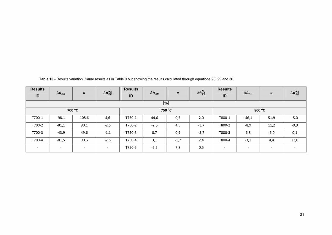
Table 10 contains the flow variations, expressed in relative terms, using equations 28, 29 and

30. The order is the same as in Table 9.

31

Table 10 - Results variation. Same results as in Table 9 but showing the results calculated through equations 28, 29 and 30.

Results

ID ∆c+ �� ½ ∆c+ ��f

Results

ID ∆c+ �� ½ ∆c+ ��f

Results

ID ∆c+ �� ½ ∆c+ ��f

%� 700 ⁰C 750 ⁰C 800 ⁰C

T700-1 -98,1 108,6 4,6 T750-1 44,6 0,5 2,0 T800-1 -46,1 51,9 -5,0

T700-2 -81,1 90,1 -2,5 T750-2 -2,6 4,5 -3,7 T800-2 -8,9 11,2 -0,9

T700-3 -43,9 49,6 -1,1 T750-3 0,7 0,9 -3,7 T800-3 6,8 -6,0 0,1

T700-4 -81,5 90,6 -2,5 T750-4 3,1 -1,7 2,4 T800-4 -3,1 4,4 23,0

- - - - T750-5 -5,5 7,8 0,5 - - - -

32

Considering Tables 9 and 10, it is seen that the 700 ⁰C case gives odd results. There are

extremely high differences between the inlet and the outlet of the AR. It is expected that some N2

leakage occurs due to the slight pressure difference between reactors and also that the oxygen

present in the AR is transported with the oxygen carrier/catalyst into the FR, however it is highly

improbable that 98 or 44% of the AR inlet flow leaks into the FR. Knowing that the FR outlet dry flow is

kept around 2 L/min and comparing all the FR inlet flows for each different temperature, is another

reason for affirming that the AR flow differences cannot be so elevated. In consequence, the

agreement between the differently calculated nitrogen flows is also low, translating into a high sigma

value.

In the experimental procedure, the system was started without introducing raw gas in the FR. At

initialization, only catalyst circulation with AR containing oxygen and nitrogen was occurring. Once the

raw gas was introduced, ilmenite was already saturated with oxygen which could not be taken into

account in the molar balance. Analyzing the O2 concentrations during the 700 ⁰C experiment, it is

visible that it has higher values than the other temperatures (e.g. 0.22% for 700 ⁰C compared to

0.02% for 800 ⁰C) and CO2 concentrations with similar magnitudes (e.g. 0.21% compared to 700 ⁰C

and 0.13 % for 800 ⁰C). This indicates that the variation in oxygen available to convert tars is a result

of the start-up procedure. Therefore, the molar balance applied is not valid for the starting

temperature, once an unknown quantity of oxygen is present in the system. Moreover, during the early

phase of the operation, which coincides with the 700 ⁰C case, the Ilmenite material used was fresh, so

not yet activated. As it is gradually activated, the system was not yet stable at the beginning of the

operation, since it needs some running time until the catalyst is totally activated. (8).

On the contrary, for the cases at higher temperature, the concentrations from the gas leaving

the AR have now lowered O2 concentrations, indicating that the oxygen entering is being transported

by the catalyst into the FR, and also that catalyst is reaching full activation.

Regarding the imposed conditions for the selection of the best data, the data possible to be

representative of each temperature is presented in Table 11.

Table 11 - Candidate data for Aspen Plus. Candidate data used in a further to create the reactor model.

Results ID ∆c+ �� ½ ∆c+ ��f Results ID ∆c+ �� ½ ∆c+ ��f

%� 750 ⁰C 800 ⁰C

T750-2 -2,6 4,5 -3,7 T800-2 -8,9 11,2 -0,9

T750-3 0,7 0,9 -3,7 T800-3 6,8 -6,0 0,1

T750-4 3,1 -1,7 2,4 T800-4 -3,1 4,4 23,0

T750-5 -5,5 7,8 0,5 - - - -

To be coherent with the selection criteria, for the 750 ⁰C case were chosen the values T750-5,

while for 800 ⁰C, the T800-4 were used.

33

Indeed, the sigma is as low as possible, the nitrogen AR flow difference has a negative value,

which allows gas leaks to occur from the AR to the FR and not otherwise, and the same for the

nitrogen increase in the FR, where the nitrogen flow is supposed to stay equal or increase.

It is clear that the sigma and AR flow change have extremely high values although the nitrogen flow

variation is within a realistic range. In the data analysis it is shown how sensitive the AR outlet flow is

with respect to the AR outlet concentrations while the FR flows remain with stable values.

Data Analysis

For the ilmenite case, the sensibility analysis will be performed for the 800 ⁰C case, starting with

results T800-4. Indeed, for the other temperatures the conclusions will be the same, because all

values have the same order of magnitude.

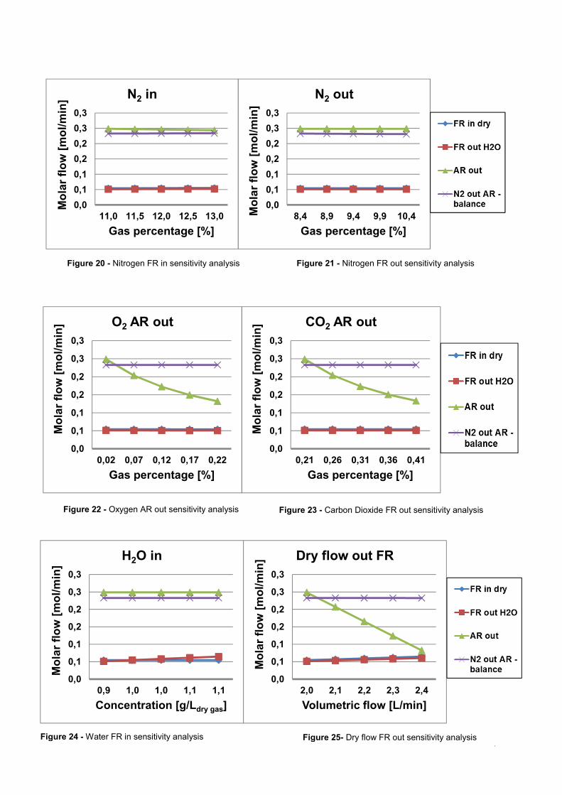
The sensitivity analysis graphs are displayed in the following Figs. 16 to 25.

Figure 16 - Hydrogen FR in sensitivity analysis Figure 17 - Hydrogen FR out sensitivity analysis

0,0

0,1

0,2

0,3

0,4

0,5

0,6

0,7

27,1 27,6 28,1 28,6 29,1

Molar flow [mol/min]

Gas percentage [%]

H2 out

0,0

0,1

0,2

0,3

22,4 22,9 23,4 23,9 24,4


Gas percentage [%]

H2 in

Figure 18 - Carbon Monoxide FR in sensitivity analysis

Figure 19 - Carbon Monoxide FR out sensitivity analysis

0,0

0,1

0,2

0,3

0,4

0,5

32,4 32,9 33,4 33,9 34,4


Gas percentage [%]

CO in

-0,2

-0,1

0,0

0,1

0,2

0,3

9,1 9,6 10,1 10,6 11,1


Gas percentage [%]

CO out

34

Figure 20 - Nitrogen FR in sensitivity analysis Figure 21 - Nitrogen FR out sensitivity analysis

0,0

0,1

0,1

0,2

0,2

0,3

0,3

8,4 8,9 9,4 9,9 10,4Molar flow [mol/min]

Gas percentage [%]

N2 out

0,0

0,1

0,1

0,2

0,2

0,3

0,3

11,0 11,5 12,0 12,5 13,0


Gas percentage [%]

N2 in

Figure 22 - Oxygen AR out sensitivity analysis Figure 23 - Carbon Dioxide FR out sensitivity analysis

0,0

0,1

0,1

0,2

0,2

0,3

0,3

0,21 0,26 0,31 0,36 0,41


Gas percentage [%]

CO2 AR out

0,0

0,1

0,1

0,2

0,2

0,3

0,3

0,02 0,07 0,12 0,17 0,22


Gas percentage [%]

O2 AR out

Figure 24 - Water FR in sensitivity analysis Figure 25- Dry flow FR out sensitivity analysis

0,0

0,1

0,1

0,2

0,2

0,3

0,3

0,9 1,0 1,0 1,1 1,1


Concentration [g/Ldry gas]

H2O in

0,0

0,1

0,1

0,2

0,2

0,3

0,3

2,0 2,1 2,2 2,3 2,4


Volumetric flow [L/min]

Dry flow out FR

35

It is seen from the figures 16 to 25 that the most sensitive result is the total AR outlet flow. This

is easily explained by the fact that when solving the molar balance, the numeric coefficients associated

(CO2 and O2 concentrations out of the AR) with this unknown are 1 or 2 orders of magnitude lower

than the remaining ones. Therefore, a slight variation in the input values causes a higher change in

this value. Nevertheless, this value is not a critical result for the Aspen Plus model, as only the FR is

mainly being considered.

The important flows for the software implementation (FR inlet dry flow and FR outlet H2O flow)

are clearly more stable and have a low response to changes in the input values. There might be cases

where e.g. the “H2O” in and the “dry flow out FR” flows change but this is because they have a more

direct relation with the input values. If these inputs increase it is obvious that the inlet flow and the

water flow in increase as well because a balance is being applied.

The error for the FR dry gases concentrations is 1% and for the other measurements they are

difficult to define (e.g., tar concentration, H2O concentration, etc.) It is also important to mention that

the AR out concentrations have a tendency to show rather high errors as the values measured with

the NDIR were critically near the detection limit.

Even with the errors associated with the measurements, it is viable to use the results to improve

the ASPEN model, once again, because the errors and changes that they might involve correspond to

a low alteration upon the results needed for implementation.

Generally, changing the carbon containing elements concentration has always a notable

influence on the total flow leaving the AR, as well as the oxygen flow entering in the AR. This happens,

as explained before, because the latter unknown is associated to a very low numerical coefficient.

4.2. Aspen and Balance Comparison

In this section are displayed all the Aspen Plus results, including all the simplification mentioned

before, with further comparison from the values obtained with the molar balance. It is important not to

forget that the simulations consider a single reactor so, all the components that in the real system

enter through different inlets (helium derived from the LS and oxygen transported into the FR with the

catalyst) are inserted in the simulation reactor through one single inlet.

It is important to mention that the only two equations were considered in the simulations: water-

gas shift and steam tar reforming.

For the temperature approach and the plug flow reactor, the model optimization is done using

the steam reforming reaction, by fitting the outlet model tar flow with the outlet tar flow obtained from

the measurements.

The results are obtained using the reactors displayed in section 1.2.

36

60% Ilmenite, 40% Silica-sand and 1% oxygen in AR

Table 12 shows the variations that occurred in the experimental facility.

Table 12 - Component molar FR balance results. In and outlet flows of the measured data.

In the molar balance it is possible to view how the flows vary after passing through the CLR

reactor. The propane is totally converted and around 87% of the acetylene is converted as well,

independently of the temperature. Table 13 displays the results obtained simulating the Gibbs reactor.

Temperature 750 ⁰C 800 ⁰C

·¸¹º ·»¼⁄ � Flows

In Out ∆µ�}�c¶®

%� In Out ∆µ�}�c¶®

%� c+ df 0,01363 0,02159 58 0,01247 0,02420 94

c+ bg 0,01969 0,00935 -52 0,01801 0,00811 -55

c+ bgf 0,00915 0,01981 117 0,00837 0,02013 141

c+ bdq 0,00740 0,00753 2 0,00677 0,00714 6

c+ bfdf 0,00022 0,00003 -88 0,00020 0,00003 -86

c+ bfdq 0,00256 0,00245 -4 0,00234 0,00173 -26

c+ bfd¯ 0,00023 0,00024 3 0,00021 0,00007 -67

c+ btd° 0,00012 0,00000 -100 0,00011 0,00000 -100

c+ �f 0,00667 0,00667 0 0,00610 0,00746 22

c+ gf±�|e�� 0,00188 0,00000 -100 0,00187 0,00000 -100

c+ ��~ 0,00028 0,00026 -8 0,00026 0,00018 -30

c+ dfg 0,06726 0,05952 -11 0,06153 0,05119 -17

c+ d® 0,02162 0,02162 0 0,02040 0,02040 0

37

Table 13 - Gibbs reactor results. Flows obtained from the model using a Gibbs reactor and comparison

with the experimental flows showed in Table 12.

It is clearly visible that the Gibbs rector flow variations vary significantly from the experiment.

Therefore it cannot be used as a basis to represent of the CLR system.

The simulation with the Equilibrium reactor and water-gas shift and tar steam reforming

equations implemented gives the results in Table 14.


·¸¹º ·»¼⁄ � Flows

In Out ∆¾kµµ~

%� ∆µ�}�c¶®

%� In O

ut

∆¾kµµ~

%� ∆µ�}�c¶®

%� c+ df 0,01363 0,06105 348 58 0,01247 0,05448 337 94

c+ bg 0,01969 0,02380 21 -52 0,01801 0,02311 28 -55

c+ bgf 0,00915 0,02154 135 117 0,00837 0,01845 120 141

c+ bdq 0,00740 0,00008 -99 2 0,00677 0,00002 -100 6

c+ bfdf 0,00022 0,00000 -100 -88 0,00020 0,00000 -100 -86

c+ bfdq 0,00256 0,00000 -100 -4 0,00234 0,00000 -100 -26

c+ bfd¯ 0,00023 0,00000 -100 3 0,00021 0,00000 -100 -67

c+ btd° 0,00012 0,00000 -100 -100 0,00011 0,00000 -100 -100

c+ �f 0,00667 0,00667 0 0 0,00610 0,00610 0 22

c+ gf±�|e�� 0,00188 0,00000 -100 -100 0,00187 0,00000 -100 -100

c+ ��~ 0,00028 0,00000 -100 -8 0,00026 0,00000 -100 -30

c+ dfg 0,06726 0,04212 -37 -11 0,06153 0,04001 -35 -17

c+ d® 0,02162 0,02162 0 0 0,02040 0,02040 0 0

38

Table 14 - Equilibrium reactor results without temperature approach. Flows obtained from the model using

equilibrium reactors and comparison with the experimental flows showed in Table 12.

The calculated values are still very different from the experimental values. The tars are

completely reformed because naphthalene is the representative compound, while in reality tars are a

mix of different compounds, with naphthalene being only one of them.

In order to overcome this, the temperature approach methodology (section 4.5.) was applied to

find a temperature difference (∆T), and match the stream values. The concept of how the temperature

approach works within ASPEN and in the reactor is explained in section 2.4. The results read are

presented in Table 15.


·¸¹º ·»¼⁄ � Flows

In Out ∆¿n. %�

∆µ�}�c¶®

%� In Out ∆¿n. %�

∆µ�}�c¶®

%� c+ df 0,01363 0,03028 122 58 0,01247 0,02688 116 94

c+ bg 0,01969 0,00976 -50 -52 0,01801 0,00984 -45 -55

c+ bgf 0,00915 0,02188 139 117 0,00837 0,01914 129 141

c+ bdq 0,00740 0,00740 0 2 0,00677 0,00677 0 6

c+ bfdf 0,00022 0,00022 0 -88 0,00020 0,00020 0 -86

c+ bfdq 0,00256 0,00256 0 -4 0,00234 0,00234 0 -26

c+ bfd¯ 0,00023 0,00023 0 3 0,00021 0,00021 0 -67

c+ btd° 0,00012 0,00012 0 -100 0,00011 0,00011 0 -100

c+ �f 0,00667 0,00667 0 0 0,00610 0,00610 0 22

c+ gf±�|e�� 0,00188 0,00188 0 -100 0,00187 0,00187 0 -100

c+ ��~ 0,00028 0,00000 -100 -8 0,00026 0,00000 -100 -30

c+ dfg 0,06726 0,05173 -23 -11 0,06153 0,04816 -22 -17

c+ d® 0,02162 0,02162 0 0 0,02040 0,02040 0 0

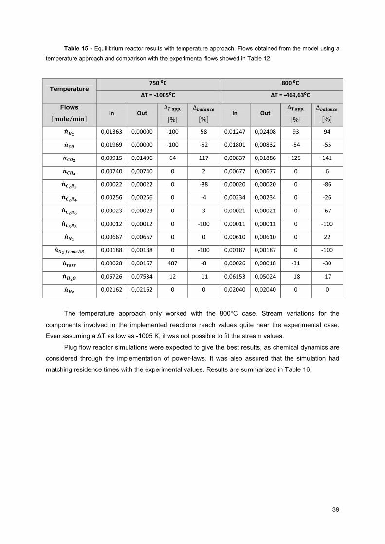
39

Table 15 - Equilibrium reactor results with temperature approach. Flows obtained from the model using a

temperature approach and comparison with the experimental flows showed in Table 12.

The temperature approach only worked with the 800⁰C case. Stream variations for the

components involved in the implemented reactions reach values quite near the experimental case.

Even assuming a ∆T as low as -1005 K, it was not possible to fit the stream values.

Plug flow reactor simulations were expected to give the best results, as chemical dynamics are

considered through the implementation of power-laws. It was also assured that the simulation had

matching residence times with the experimental values. Results are summarized in Table 16.


ΔT = -1005⁰C ΔT = -469,63⁰C

·¸¹º ·»¼⁄ � Flows

In Out ∆À.�mm. %�

∆µ�}�c¶®

%� In Out ∆À.�mm. %�

∆µ�}�c¶®

%� c+ df 0,01363 0,00000 -100 58 0,01247 0,02408 93 94

c+ bg 0,01969 0,00000 -100 -52 0,01801 0,00832 -54 -55

c+ bgf 0,00915 0,01496 64 117 0,00837 0,01886 125 141

c+ bdq 0,00740 0,00740 0 2 0,00677 0,00677 0 6

c+ bfdf 0,00022 0,00022 0 -88 0,00020 0,00020 0 -86

c+ bfdq 0,00256 0,00256 0 -4 0,00234 0,00234 0 -26

c+ bfd¯ 0,00023 0,00023 0 3 0,00021 0,00021 0 -67

c+ btd° 0,00012 0,00012 0 -100 0,00011 0,00011 0 -100

c+ �f 0,00667 0,00667 0 0 0,00610 0,00610 0 22

c+ gf±�|e�� 0,00188 0,00188 0 -100 0,00187 0,00187 0 -100

c+ ��~ 0,00028 0,00167 487 -8 0,00026 0,00018 -31 -30

c+ dfg 0,06726 0,07534 12 -11 0,06153 0,05024 -18 -17

c+ d® 0,02162 0,02162 0 0 0,02040 0,02040 0 0

40

Table 16 - Plug flow reactor with Naphthalene power law values. Flows obtained from the model using a

plug flow reactor with kinetic data for Naphthalene kinetic data and comparison with the experimental flows

showed in Table 12.

No tars are reformed using the chemical constant for naphthalene. Therefore, the iterative

process described in section 4.5. is used to calculate a chemical constant that induces reforming. The

results are shown in Table 17.


·¸¹º ·»¼⁄ � Flows

In Out ∆yb°dsh

%� ∆µ�}�c¶®

%� In Out ∆yb°dsh

%� ∆µ�}�c¶®

%� c+ df 0,01363 0,02399 76 58 0,01247 0,02099 68 94

c+ bg 0,01969 0,00933 -53 -52 0,01801 0,00950 -47 -55

c+ bgf 0,00915 0,01951 113 117 0,00837 0,01688 102 141

c+ bdq 0,00740 0,00740 0 2 0,00677 0,00677 0 6

c+ bfdf 0,00022 0,00022 2 -88 0,00020 0,00020 1 -86

c+ bfdq 0,00256 0,00256 0 -4 0,00234 0,00234 0 -26

c+ bfd¯ 0,00023 0,00023 -2 3 0,00021 0,00021 -2 -67

c+ btd° 0,00012 0,00012 -2 -100 0,00011 0,00011 -2 -100

c+ �f 0,00667 0,00667 0 0 0,00610 0,00610 0 22

c+ gf±�|e�� 0,00188 0,00188 0 -100 0,00187 0,00187 0 -100

c+ ��~ 0,00028 0,00028 0 -8 0,00026 0,00026 0 -30

c+ dfg 0,06726 0,05690 -15 -11 0,06153 0,05302 -14 -17

c+ d® 0,02162 0,02162 0 0 0,02040 0,02040 0 0

41

Table 17 - Plug flow reactor with ktars found through iterative process. Flows obtained from the model using

a plug flow reactor with kinetic data obtained iteratively and comparison with the experimental flows showed in

Table 12.

Adapting the tar kinetics to the real outlet flow, gives ASPEN values that are not similar but

follow the trend verified for the experimental results at a high rate. The streams that proceed from

methane to propane in the previous tables, do not match at any level the experimental results, as

expected, because no reaction involving them was included. Nevertheless, their stream value is one

order of magnitude lower than the stream values from the components included in reactions and

therefore the influence on the total flow value is low.

In the case of nitrogen, leakage from the AR to the FR explains why the stream increases in the

balance case, while in the model it remains constant.

In conclusion, it is possible to affirm that for the tested hypothesis, the plug flow with the

adapted chemical constant for both temperatures and the equilibrium reactor with temperature

approach for 800 ⁰C describe the FR more accurately.


y = ¯ × shsÁeh,tye|}_h,s~_s y = q, Á × shsÁeh,tye|}_h,s~_s

·¸¹º ·»¼⁄ � Flows

In O

ut

∆yk�®�. %�

∆µ�}�c¶®

%� In Out ∆yk�®�. %�

∆µ�}�c¶®

%� c+ df 0,01363 0,02429 78 58 0,01247 0,02216 78 94

c+ bg 0,01969 0,00950 -52 -52 0,01801 0,01023 -43 -55

c+ bgf 0,00915 0,01953 114 117 0,00837 0,01695 102 141

c+ bdq 0,00740 0,00740 0 2 0,00677 0,00677 0 6

c+ bfdf 0,00022 0,00022 0 -88 0,00020 0,00020 0 -86

c+ bfdq 0,00256 0,00256 0 -4 0,00234 0,00234 0 -26

c+ bfd¯ 0,00023 0,00023 0 3 0,00021 0,00021 0 -67

c+ btd° 0,00012 0,00012 0 -100 0,00011 0,00011 0 -100

c+ �f 0,00667 0,00667 0 0 0,00610 0,00610 0 22

c+ gf±�|e�� 0,00188 0,00188 0 -100 0,00187 0,00187 0 -100

c+ ��~ 0,00028 0,00026 -8 -8 0,00026 0,00018 -31 -30

c+ dfg 0,06726 0,05668 -16 -11 0,06153 0,05216 -15 -17

c+ d® 0,02162 0,02162 0 0 0,02040 0,02040 0 0

42

4.3. Energetic Assessment

60% Ilmenite / 40% Silica-sand and 1% oxygen in AR

For energetic calculations only the simulations that give similar results and trends in comparison

to the experimental values are used (plug flow with the adapted chemical constant for both

temperatures and the equilibrium reactor with temperature approach for 800 ⁰C). For this reason, only

the Ilmenite case is evaluated, using the experimental data and the simulation results and by

“combusting” the following chemical energy carriers: H2, CO, CH4, C2H2, C2H4, C2H6, C3H8 at the inlet

and the outlet. Results are shown in Table 18.

Table 18 - Chemical energy loss assessment. Results of the heat value variation assessment explained in

section 3.6.

In the experimental results and considering the mentioned chemical energy carriers, it is

possible to conclude that a loss occurs in both cases. On the other hand, the same trend is only visible

in the plug flow for 750 ⁰C but is still not as high as the experimental values. For the 750 ⁰C the trend

is not followed at all. There is even an increase in chemical energy. The explanation relies in the fact

that in the modeling only hydrogen was considered to take part in reactions. The other possible energy

carrier flows remained unaltered. When comparing the molar flows, it seems to have no major

influence as the flow value is one order of magnitude lower than the higher flows. So, from this short

comparison, it is possible to verify that at an energetic level their contribution has to be taken into

account. For e.g. when looking at the molar flow results, acetylene and propane are almost totally

oxidized, while in the model not.

Conditions 750 ⁰C 800 ⁰C

25⁰C and 1 bar Molar

balance

Plug flow with

adapted k

Molar

balance

Plug flow with

adapted k

Temperature

approach

∆d¶kc}®��~®~fÂ°Ã Ä�� 317,4 290,3

∆d¶|��}®��~®~fÂ°Ã Ä�� 292,2 312,3 271,7 292,7 291,4

∆dbÅ� [%] -8,0 -1,6 -6,4 0,8 0,4

43

5. Closure

5.1. Conclusions

The Ilmenite results were appropriate to use for ASPEN implementation. Coherent results

between experimental values and simulations were obtained.

It is clearly visible how the AR flow out is sensitive to variation of molar balance input values.

87% of the acetylene and 100% of propane are oxidized and this trend seems to be

independent of temperature. Unfortunately at 700⁰C results are unclear and so it is not possible to

assess if the same trend can be applied in a general way for these system operative conditions.

Generally, methane doesn’t suffer high flow variations, independently of the temperature.

At a molar balance level, it seemed reasonable only to include two reactions, tar steam

reforming and water-gas shift, leading to values that follow the same trend values and are often quite

similar comparing to the experimental results. However, when doing the energy analysis in section 5.4,

it is verified that the flows in the model not included in any reaction, probably oxidation reactions,

cannot be left out. Actually there is a chemical energy loss, while in the models they are low or there

can even be an increase. This indicates that more reactions related to the main chemical energy

carriers that initially were not considered have to be implemented, in order to make the model fit not

only at a molar balance level but also in energetic terms.

It was only possible to elaborate a coarse model for each system condition. The described

methodologies were applied for each condition and always different system descriptive values were

obtained (e.g. chemical constant for tar breakdown and ∆T from temperature approach). Elaborating a

CLR model that covers all possible system conditions remains a laborious task. Detailed knowledge

about the system reaction kinetics (tar reforming, catalyst kinetics, equilibrium reactions involved, etc.)

needs deeper investigation.

5.2. Suggestions for Further Work

The proposed model and methodology should be tested with more measurements obtained

from the CLR system. Around 70-80% of the fluidizing helium leaves the system through the FR and

these values are also almost reached with the made assumptions (Appendix VI). Applying the balance

knowing beforehand how the helium is distributed between the reactors could also be a further

improvement to the model.

Another important upgrade to the model would be the implementation of oxidization reactions

for the considered chemical energy carriers, in order to fit both energy balances, from the models and

the experimental data.

44

Finally, it should be attempted to implement in the Aspen Plus model the more complex tar

decomposition scheme elaborated in the master thesis “Development of a tar decomposition model for

application in a chemical-looping reformer operated with raw gas from a biomass gasifier”.

45

References

1. Coll, R., et al. Steam reforming model compounds of biomass gasification tars: conversion

at different operating conditions and tendency towards coke formation. Fuel Processing Technology.

2001, Vol. 74, pp. 19-31.

2. Swierczynski, D., et al. Study of steam reforming of toluene used as model compound of

tar produced by biomass gasification. Chemical Engineering and Processing: Process Intensification.

2007, Vol. 47, pp. 508-513.

3. Dabai, F., et al. Tar Formation and Destruction in a Fixed-Bed Reactor Simulating

Downdraft Gasification: Equipment Development and Characterization of Tar-Cracking Products.

Energy & Fuels. 2010, Vol. 24, pp. 4560–4570.

4. Bridgwater, A. The technical and economic feasibility of biomass gasification for power

generation. Renewable and Sustainable Energy Reviews. 1995, Vol. 74, pp. 631-653.

5. Heyne, S. Process Integration Opportunities for Synthetic Natural Gas (SNG) Production by

Thermal Gasification of Biomass. Chalmers University of Technology, 2010.

6. Torres, W., et al. Hot Gas Removal of Tars, Ammonia, and Hydrogen Sulfide from Biomass

Gasification Gas. 2007, Vol. 49, pp. 407 — 456.

7. Swierczynski, D., et al. Steam reforming of tar from a biomass gasification process over

Ni/olivine catalyst using toluene as a model compound. 2007, Vol. 74, pp. 211-222.

8. Lind, F., et al. Continuous Catalytic Tar Reforming of Biomass Derived Raw Gas

Simultaneous Catalyst Regenertation. Chalmers University of Technology, 2011.

9. Li, C., et al. Tar property, analysis, reforming mechanism and model for biomass

gasification—An overview. 2009, Vol. 13, pp. 594-604.

10. Milne, T., et al. Biomass Gasifier “Tars”: Their Nature, Formation and Conversion. National

Renewable Energy Laboratory, 1998.

11. Hayes, R., et al. A study of the nickel-catalyzed methanation reaction. Journal of Catalysis.

2, 1985, Vol. 92, pp. 312-326.

12. Rapagnà, S., et al. Steam-gasification of biomass in a fluidised-bed of olivine particles.

Biomass and Bioenergy. 2000, Vol. 19, pp. 187-197.

13. Simell, P. Effects of gasification gas components on tar and ammonia decomposition over

hot gas cleanup catalysts. Fuel. Elsevier Ltd., 1997, Vol. 76, pp. 1117-1127.

14. Mendiara, T. Chemical Looping Reforming of Generator Gas. Department of Chemical and

Biomchemical Engineering. Technical University of Denmark, 2009.

15. Aspen Technology. Getting Started Building and Running a Process Model. Aspen

Technology, 2007.

16. Van Ness, H., et al. Thermodynamics. [book auth.] R. Perry and D. Green. Perry's

Chemical Engineers' Handbook. 7th. McGraw-Hill, 1997.

17. Dayton, D. A Review of the Literature on Catalytic Biomass Tar Destruction. National

Renewable Energy Laboratory, 2002.

46

18. Fjellerup, J., et al. Formation, Decomposition and Cracking of Biomass Tars in Gasification.

Technical University of Denmark, 2005.

19. Taralas, G., et al. Modeling the Thermal Destruction of Toluene (C7H8) as Tar-Related

Species for Fuel Gas Cleanup. Energy Fuels. 2003, Vol. 17, pp. 329-337.

20. Corella, J., et al. Biomass Gasification with Air in Fluidized Bed: Reforming of the Gas

Composition with Commercial Steam Reforming Catalysts. 1998, Vol. 37, pp. 4617-4624.

21. Lind, F. Catalytiv tar cleaning of biomass-derived gas with simultaneous caltalyst

regeneration. Chalmers University of Technology, 2011.

22. Narváez, I., et al. Fresh Tar (from a Biomass Gasifier) Elimination over a Commercial

Steam-Reforming Catalyst. Kinetics and Effect of Different Variables of Operation. American Chemical

Society, 1997, Industrial & Engineering Chemistry Research, Vol. 36, pp. 317-327.

23. Corella, J., et al. Improving the Modeling of the Kinetics of the Catalytic Tar Elimination in

Biomass Gasification. Industrial & Engineering Chemistry Research. American Chemical Society,

2002, Vol. 41, pp. 3351-3356.

24. Ryden, M., et al. Synthesis gas generation by chemical-looping reforming in a continuously

operating laboratory reactor. Fuel. 2006, Vol. 85, pp. 1631-1641.

25. Thunman, H., et al. Tar Cleaning with Chemical Looping Reforming.

26. Walas, S. Reaction Kinetics. [book auth.] R. Perry and D. Green. Perry's Chemical

Engineers' Handbook. 7th. McGraw-Hill, 1997.

47

Appendix I – MatLab file for the molar balance

%========================================================================= % % BALANCES % %========================================================================= clear all clc % CALL THE EXCEL FILE filename = 'Concentrations_for_MatLab.xls'; open = xlsread(filename); % SPECIES CONCENTRATIONS [%mol] conc_FR_in = open(91:107,29:39); %[H2,CO,CO2,CH4,C2H2,C2H4,C2H6,C3H8,N2] size_FR_in = size(conc_FR_in); conc_FR_out_700 = open(11:28,29:39); %[H2,CO,CO2,CH4,C2H2,C2H4,C2H6,C3H8,N2,O2,He] size_FR_700 = size(conc_FR_out_700); conc_FR_out_750 = open(34:53,29:39); %[H2,CO,CO2,CH4,C2H2,C2H4,C2H6,C3H8,N2,O2,He] size_FR_750 = size(conc_FR_out_750); conc_FR_out_800 = open(59:72,29:39); %[H2,CO,CO2,CH4,C2H2,C2H4,C2H6,C3H8,N2,O2,He] size_FR_800 = size(conc_FR_out_800); conc_AR_out_700 = open(118:3564,4:5); %[CO2,O2] size_AR_700 = size(conc_AR_out_700); conc_AR_out_750 = open(3564:7185,4:5); %[CO2,O2] size_AR_750 = size(conc_AR_out_750); conc_AR_out_800 = open(7186:9829,4:5); %[CO2,O2] size_AR_800 = size(conc_AR_out_800); H2O_in = open(14,43); % [g/l] Tars_in = open(9,43); % [g/l] Tars_out_700 = open(9,44); % [g/l] Tars_out_750 = open(27,44); % [g/l] Tars_out_800 = open(45,44); % [g/l] % FLOWS v_dry_out = open(14,44); % [l/min] He_SLS = open(60,44); % [l/min] He_ILS = open(61,44); % [l/min] He_in = He_SLS+He_ILS; % [l/min] O2_AR_in = open(65,44); % [l/min] N2_AR_in = open(66,44); % [l/min] clear open

48

% Constants %Molar Volume Vm = 22.4; %[l/mole] %Molar weights H2 = 2; %[g/mole] CO = 28; %[g/mole] CO2 = 44; %[g/mole] CH4 = 16; %[g/mole] C2H2 = 26; %[g/mole] C2H4 = 28; %[g/mole] C2H6 = 30; %[g/mole] C3H8 = 44; %[g/mole] N2 = 28; %[g/mole] O2 = 32; %[g/mole] H2O = 18; %[g/mole] %Considering Naphtalene(C10H8) Tars = 128; %[g/mole] %Moles of each species in each molecules %[H2,CO,CO2,CH4,C2H2,C2H4,C2H6,C3H8,N2,O2,He] %Carbon moles_C = [0 1 1 1 2 2 2 3 0 0 0]; %Hidrogen moles_H = [2 0 0 4 2 4 6 8 0 0 0]; %Oxygen moles_O = [0 1 2 0 0 0 0 0 0 2 0]; %Nitrogen moles_N = [0 0 0 0 0 0 0 0 2 0 0]; % CALCULATIONS %Average FR input concentration av_con_FR_in = sum(conc_FR_in,1)/size_FR_in(1,1); %%%%%%%%%%%%%%%%%%%%%%%%%%%%%%%%%%%%%%%%%%%%%%%%%%%%%%%%%%%%%%%%%%%%%%%%%¤ %LOOPS TO FIND OUT n_FR_in_dry, n_FR_out_H2O and n_AR_out (molar flows) %%%%%%%%%%%%%%%%%%%%%%%%%%%%%%%%%%%%%%%%%%%%%%%%%%%%%%%%%%%%%%%%%%%%%%%%%% % Matrix M and vector a M = [0 0 0 ; 0 -2 0 ; 0 -1 0 ]; a = zeros(3,1); %Auxiliar vector for in FR concentrations inFR = av_con_FR_in; %Creates Excel file to write results Matrix_scheme = {'[mol/min],[%mol/mol] and [-]' 'H2' 'CO' 'CO2' 'CH4' 'C2H2' 'C2H4' 'C2H6' 'C3H8' 'N2'...

49

'O2 from AR' 'He' 'Tars' 'H2O' 'Dry flow(out is with He)' 'Humid flow(out is with He)'... 'C' 'H' 'O' 'N' 'AR' 'N2 AR out-balance' 'N2 AR out-He' 'sigma' '[CO2 out AR]' '[O2 out AR]' 'location FR out list' 'location AR out list'}; xlswrite('Flow Results',Matrix_scheme,'700','A1'); xlswrite('Flow Results',Matrix_scheme,'750','A1'); xlswrite('Flow Results',Matrix_scheme,'800','A1'); Matrix_scheme = {'Average in Concentrations[%]'}; xlswrite('Flow Results',Matrix_scheme,'700','A3'); xlswrite('Flow Results',Matrix_scheme,'750','A3'); xlswrite('Flow Results',Matrix_scheme,'800','A3'); xlswrite('Flow Results',inFR,'700','B3'); xlswrite('Flow Results',inFR,'750','B3'); xlswrite('Flow Results',inFR,'800','B3'); Matrix_scheme = {'Flow in FR[mol/min]'}; xlswrite('Flow Results',Matrix_scheme,'700','A5'); xlswrite('Flow Results',Matrix_scheme,'750','A5'); xlswrite('Flow Results',Matrix_scheme,'800','A5'); Matrix_scheme = {'Flow out FR[mol/min]'}; xlswrite('Flow Results',Matrix_scheme,'700','A6'); xlswrite('Flow Results',Matrix_scheme,'750','A6'); xlswrite('Flow Results',Matrix_scheme,'800','A6'); Matrix_scheme = {'[Concentrations out FR(1-9,11),AR(21-22) and N2 balance out AR[mol/min]]'}; xlswrite('Flow Results',Matrix_scheme,'700','A7'); xlswrite('Flow Results',Matrix_scheme,'750','A7'); xlswrite('Flow Results',Matrix_scheme,'800','A7'); %%%%%%%%%%%%%%%%%%%%%%%%%%%%%%%%%%%%%%%%%%%%%%%%%%%%%%%%%%%%%%%%%%%%%%%%%% % loop for 700 degrees Celsius Tars_out = Tars_out_700; %Result matrix and auxiliar writing variable results700 = zeros(size_FR_700(1,1)*size_AR_700(1,1),7); Results_Excel = zeros(1,24); h = 0; k = 0; calc_dec = 0; for i = 1:size_FR_700(1,1) %Auxiliar vector for out FR concentrations outFR = conc_FR_out_700(i,:); %jumps AR concentrations as they repeat itself

50

for j = 1:2:size_AR_700(1,1) %Auxiliar vector for out AR concentrations outAR = conc_AR_out_700(j,:); calc_dec = calc_dec-sum(outAR); if calc_dec ~= 0 calc_dec = sum(outAR); %Carbon balance coeficients M(1,1) = (inFR*moles_C')/100 + 10*Tars_in*Vm/Tars; M(1,3) = -outAR(1)/100; a(1,1) = (v_dry_out/Vm)*((outFR*moles_C')/100 + 10*Tars_out*Vm/Tars); %Hidrogen balance coeficients M(2,1) = (inFR*moles_H')/100 + 8*Tars_in*Vm/Tars + 2*H2O_in*Vm/H2O; a(2,1) = (v_dry_out/Vm)*((outFR*moles_H')/100 + 8*Tars_out*Vm/Tars); %Oxigen balance coeficients M(3,1) = (inFR*moles_O')/100 + H2O_in*Vm/H2O; M(3,3) = -2*(outAR(1)+outAR(2))/100; a(3,1) = (v_dry_out/Vm)*(outFR*moles_O')/100 - 2*O2_AR_in/Vm; %Calculates flows n = M\a; %Writes realistic results if n(3) > 0 h = h+1; results700(h,1) = n(1); results700(h,2) = n(2); results700(h,3) = n(3); %AR flow out with different units [l/m] results700(h,4)=n(3)*Vm; %AR flow in to compare with AR flow out result results700(h,5)=(He_SLS+He_ILS)*(1-outFR(11)/100)+O2_AR_in+N2_AR_in; %Writes location of AR_out and FR_out results700(h,6)=i;

51

results700(h,7)=j; %Writes results and information into excel file [n/min]- line 1 in and line 2 out k = k+1; Results_Excel(k,1:11) = inFR*n(1)/100; Results_Excel(k,10) = O2_AR_in/Vm-n(3)*(sum(outAR))/100; Results_Excel(k,11) = (outFR(11)/100)*v_dry_out/Vm; Results_Excel(k,12) = n(1)*Tars_in*Vm/Tars; Results_Excel(k,13) = n(1)*H2O_in*Vm/H2O; Results_Excel(k,14) = sum(Results_Excel(k,1:9))+Results_Excel(k,10)... +Results_Excel(k,12); Results_Excel(k,15) = Results_Excel(k,14)+Results_Excel(k,13); Results_Excel(k,16) = Results_Excel(k,1:11)*moles_C'... +10*Results_Excel(k,12); Results_Excel(k,17) = Results_Excel(k,1:11)*moles_H'... +8*Results_Excel(k,12)+2*Results_Excel(k,13); Results_Excel(k,18) = Results_Excel(k,1:11)*moles_O'... +Results_Excel(k,13); Results_Excel(k,19) = Results_Excel(k,1:11)*moles_N'; Results_Excel(k,20) = ((He_SLS+He_ILS)*(1-outFR(11)/100)+O2_AR_in... +N2_AR_in)/Vm; k = k+1; Results_Excel(k,1:11) = outFR*(v_dry_out/Vm)/100; Results_Excel(k,10) = 0; Results_Excel(k,11) = (outFR(11)/100)*v_dry_out/Vm; Results_Excel(k,12) = (v_dry_out/Vm)*Tars_out*Vm/Tars; Results_Excel(k,13) = n(2); Results_Excel(k,14) = sum(Results_Excel(k,1:9))+Results_Excel(k,10)... +Results_Excel(k,11)+Results_Excel(k,12); Results_Excel(k,15) = Results_Excel(k,14)+Results_Excel(k,13); Results_Excel(k,16) = Results_Excel(k,1:11)*moles_C'... +10*Results_Excel(k,12); Results_Excel(k,17) = Results_Excel(k,1:11)*moles_H'... +8*Results_Excel(k,12)+2*Results_Excel(k,13); Results_Excel(k,18) = Results_Excel(k,1:11)*moles_O'... +Results_Excel(k,13); Results_Excel(k,19) = Results_Excel(k,1:11)*moles_N'; Results_Excel(k,20) = n(3); k = k+1; %Writes FR and AR out concentrations and [mol/min] N2 balance Results_Excel(k,1:11) = outFR; Results_Excel(k,21) = (N2_AR_in/Vm+inFR(9)*n(1)/100)-... outFR(9)*v_dry_out/(100*Vm); Results_Excel(k,22) = n(3)*(1-sum(outAR)/100)-... (He_in-v_dry_out*(1-sum(outFR)/100))/Vm; Results_Excel(k,23) = (1-Results_Excel(k,22)/...

52

Results_Excel(k,21))*100; Results_Excel(k,24:25) = outAR; Results_Excel(k,26) = i; Results_Excel(k,27) = j; k = k+1; else end else end end end %results700 = Results_Excel; %Write in Excel file xlswrite('Flow Results',Results_Excel,'700','B5'); clear Results_Excel;

bb (Note: Code only for 700 ⁰C is shown, as for the other temperatures it is the same.)

53

Appendix II – Typical MatLab input Excel file

FR

outlet

valu

es

54

FR

inle

t valu

es

55

AR outlet values and other measured values

56

Appendix III – MatLab results example

57

Appendix IV – New Aspen Plus CLR flow-sheet

with tested reactors

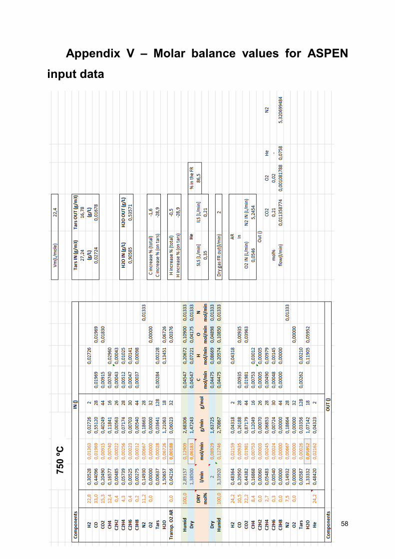
58

Appendix V – Molar balance values for ASPEN

input data

750 ºC

59

800 ºC

VP-Development of an ASPEN Plus model of a Chemical ... · Development of an ASPEN Plus Model of a...

Documents

Transcript of VP-Development of an ASPEN Plus model of a Chemical ... · Development of an ASPEN Plus Model of a...