Bulletin of Mathematical Biology, Vol. 41, pp. 229-251 Pergamon Press Ltd. 1979. Printed in Great Britain �9 Society for Mathematical Biology

0007--4985/79/0301-0229 $02.00/0

VOLTERRA-VERHULST PREY-PREDATOR SYSTEMS WITH TIME DEPENDENT COEFFICIENTS: DIFFUSION TYPE APPROXIMATION AND PERIODIC SOLUTIONS

�9 D. KANNAN Department of Mathematics, University of Georgia, Athens, Georgia 30602, U.S.A.

In treating the Volterra-Verhulst prey-predator system with time dependent coefficients, we ask how far this deterministic system represents or approximates the dynamics of the population evolving in a realistic environment which is stochastic in nature. We consider a stochastic system with small Gaussian noise type fluctuations. It is shown that the higher moments of the deviation of the deterministic system from the stochastic approach zero as the strength 6 of the perturbation decays to zero. For any <5 > 0 and all T> 0, e > 0, the sample population paths that stay within e distance from the deterministic path during [0, T] form a collection of positive probability. In comparing the stationary distributions of the two systems, we show that the weak limits of those of the stochastic system form a subset of those of the deterministic system. This is in analogy with a result of May connected with the stability of the two systems. Plant and rodent populations possess periodic parameters and exhibit periodic behavior. We establish theoretically this periodicity under periodicity conditions on the coefficients and perturbing random forces. We also establish a central limit property for the prey-predator system.

1. Introduction; the Model and Problems. Volterra's biomathematical work still constitutes the main theme of the deterministic theory of population dynamics. The pioneering basic mathematical analysis, in the 1930's, of population dynamics, by Volterra, Lotka, Kostitzin and Kolmogorov, was so comprehensive that it left very little for further work. Because of the complexity in the biosyst'ems, stochastic models are more appropriate. Based on Volterra's deterministic models, Feller ~ initiated the development of stochastic models. Almost all known stochastic models, including ours, take Volterra's model as

229

230 D. K A N N A N

the starting point. In a recent work (c.f. Kannan, 1976) we constructed a strong Markov process describing the interacted predator system which is evolving with the support of a free host population, a birth-death process. Because the environmental fluctuations and perturbations contribute substantially to the evolution of a system of competing species, we took the following approach in Gard and Kannan (1976). We considered the Volterra and Verhulst terms as regular drift and let a perturbation of white noise type act on the system. Thus we worked with a system of stochastic differential equations. In this article we continue to work with randomly perturbed Volterra-Verhulst system with further extensions and generalizations.

To discuss the problems that we consider in this article let us begin with a system of N prey and M predators governed by the Volterra equations

= xi[ai - ~ aijYa]; i = 1,..., N, i=1 (1.1)

dt = Yi - c j 7 j i x i , j = l .... ,M,

of the ith where x~(t) (respectively, yj(t)) is the size prey population (respectively, thej th predator population) at time t, a~ > 0, c i > 0, ei j> 0 and 7~ >0. Adding Pearl-Verhulst second order dissipation terms to this system, Equations (1.1) take the form

-dT=Xi a i - ~ cqjyj-eixi , i=l, . . . ,N, (1.2) j = l

dY-A= I " 1 dt yj - c j + ~ 7jix i-~,jyj , i = l

j---- 1,...,M,

where ei > 0 and 7j > 0. In these systems the environmental parameters are constants. In realistic biological systems these coefficients are both time dependent and randomly varying. This general case is the one we treat in this article. Because of their stochastic nature, the coefficients will be functions of a sample variable ~, where ~ belongs to the sample space ~2 of a supporting complete probability space (~, ~', P). In these very general terms, our stoch- astic Volterra-Verhulst system is

E J dXi_xi(t ) ai(t, co ) - ~ aij(t,~)yj(t)-o~i(t, to)xi(t) , dt j = l

dy/=yj(t)[-c '( t '~n)+~YJ'( t '")x '( t )-yJ(t 'c~ 1 " , = ~

(1.3)

V O L T E R R A - V E R H U L S T PREY PREDATOR SYSTEMS 231

The System (1.3) is too general to handle. To simplify the model a bit we can rewrite each one of the coefficients as the sum of an averaged part and a random perturbed Part. Accordingly the random parts will have zero expectations. We assume that these random parts form a collection of (possibly) correlated Gaussian noise processes with time dependent intensity. Hence, there exists a multi-dimensional Gaussian process g(t, co) with independent increments such that Eg(t, co)= 0 and the covariance matrix is given in terms of the covariances and cross-covariances of the Gaussian noise parts. But, such a Gaussian process g(t ,o) has a stochastic integral representation with respect to a Brownian motion (c.f. Gikhman and Skorokhod, 1969). Hence, under the Gaussian noise type perturbations of environmental parameters, we can rewrite the System (1.3) as follows:

dxi (t ) = Ai (t, xi, Y )dt + Si (t, xi, y )dfli( t, ~ ) (1.4)

dyj (t) = Cj (t, y j, x )dt + cr i (t, x, yj)dfl j (t, ~ ),

where (fll,"',flN) and (fll,...,flM) are two independent vector Brownian m~tions,

Ai(t, xi, y )= a i ( t ) - ~ o~ij(t)yj-o~i(t)x i xi 1=1

and

[ N 1 Cj(t,x, yj)= - c j ( t ) + ~. 7j~(t)x~-7j(t)yj Yr" i=1

Because we expressed the stochastic coefficients as the sum of averaged and random perturbed parts, the fluctuational terms Si and a) can either be taken in the same forms as Ai and Cj or in more general terms which are to satisfy certain assumptions that will be specified afterwards. For the convenience of mathematical analysis let us rewrite the deterministic .(time-dependent) Volterra-Verhulst system and our stochastic system in the ( N + M ) - dimensional vector forms as follows:

dx(t) = B(t, x( t)) (1.5) dt

d~(t, o )=B( t , ~(t, o))dt + S(r, ~(t, o))dfl(t, o), (1.6)

232 D. KANNAN

where ~(t, 09) reduces to x(t) in the deterministic case, and fl(t) is a standard vector Brownian motion. Our purpose in this article is to analyze and compare the above deterministic and stochastic systems. (At this point we would like to remark that the object we studied in Gard and Kannan (1976) was the System (1.5), and there we analyzed some stability properties along with the extinction or explosion of one or both populations and the analytical properties of the probabilities of extinction and explosion.) Here, we will work with both the deterministic and stochastic systems. One more remark is in order. We obtained the System (1.6) under the assumption of Gaussian noise type fluctuations arising in the parameters. After treating this case, we will also look at a non-Gaussian perturbation case.

In comparing the deterministic and stochastic systems, it is natural to ask an important and fundamental question that as to what extent the deterministic models do, or do not, represent the environmentally stochastic reality (c.f. May, 1974, p. 69; 1974). In a certain way of answering this problem, we further modify the stochastic system. Instead of arbitrary random perturbations we treat weak or small random perturbations. Thus, we want to study the following integral equations:

I' x(t) = xo + B(s, x(s))ds, (1.7)

d o .

f' f' r = ~o + B(s, r (s))ds + x/6 S(s, ~6(s))dfl(s), o o

(1.8)

where 3 > 0 is a small dimensionless parameter. We want to compare the deterministic evolution x(t) with the diffusion process r 09) as ~ 0 . Robert May, in his work, has compared certain deterministic models with the corresponding stochastic models. For example, he has compared the stability properties of these systems. His stochastic models also arose out of white noise type fluctuations in the environment. Our approach is through stochastic equations, and we look at different problems in addition to studying the equilibrium levels of the populations.

Equation (1.7) is a deterministic equation and (1.8) is an Ito equation. The second integral on the righthand side of (1.8) is the Ito integral. For detailed accounts of Ito integrals and equations we refer to the books by Gikhman and Skorokhod (1969, 1972) and McKean (1969). The coefficient x/-6S(s, ~a(s)) in (1.8) represents the variance part of the random environment. We will show that the distance between the deterministic and stochastic evolutions can be made arbitrarily small (as 310). In other words, we show that the variance and the higher moments of the differcnce ~a(t. ~ , ) ) -x( t )can be made very small (as the I]ttctuation is sufficicntl 5 ~vcak. 6~0). Thus the two systems (deterministic

VOLTERRA-VERHULST PREY--PREDATOR SYSTEMS 233

and stochastic) are asymptotically close to each other in a suitable sense. Let us fix a 5 >0. Let the two systems begin the evolution with the same initial population size. Consider the collection of all sample population paths which stay within an ~ distance from the deterministic population path during the time interval [0, 7]. We will show that this collection of sample paths form a collection of positive probability, for all T> 0 and e > 0.

In passing from System (1.3) to System (1.4) we made the assumption that the fluctuations are of Gaussian noise type. Next we consider general stochastic fluctuations without Gaussian noise qualifications. Thus in place of System (1.4) we have

~-[xi(t)=xi(t) a i ( t ) - ~ aij(t)yj(t)-ai(t)xi(t) j = l

+ (~fi(t, X, )', r (1 .9)

dr- y~(t) - yj(t) - cj(t) ~ 7ji(t)xi(t) - ~/j(t)yj(t) i=1

+(~gj(t,x,y,o~),

where ~ > 0 is a dimensionless parameter denoting the strength of fluctuation. We rewrite I1.9) as an (N + M)-dimensional vector equation. Set

and

Then,

X (t) -~ (x I ( t ) . . . . , xN(t), Yl (t),..., YM(t))*,

B(t .X (t))=diagonal al ( t ) - ~ eijyj(t)-~l(t)xl(t) . . . . , j = l

- c , ( t ) + ~, ' / , i( t)xi(t)-7.(t)y,(t) , i=1

F(t, X( t ) , o)) -- ( j ; ( t , x, y, 6o) , . . . , fN, g l , . . . , gM( t, X, y, (D))*.

d ~t x (t) = B(t, X (t))X (t) + bF(t, X (t), ~). (1.10)

234 D. KANNAN

We reduce (1.10) to a standard form by a nonlinear transformation

X(t)=exp{ f'oB(S,X(s))ds} 4(t). (1.11)

Equation (1.10) reduces to

d d t ~(t)-b~I)(t, ~(t), t~) (1.12)

where

�9 (t,~(t),~o)=F(t,X(t),t~)exp{-ffoB(S,X(s))ds }

and X(t), ~(t) are connected by (1.11). Let r be the solution of (1.12). We get a deterministic system

d~~ =0~ ~ (1.13) dt

by averaging ~(t, ~(t), ~n) over the time and sample space. Equation (1.12) and (1.13) are the systems we work with next. We mainly show, under suitable restrictions, that the stochastic system satisfies a central limit property; that is, the system ~a(t, Cn) centered at ~~ and normalized by ~1/2 (i.e., 6- ~/2[~6(t, co) - 4 ~ (t)]) converges weakly to a diffusion process r/(t, to).

The existence of equilibrium level is of basic importance in population dynamics. So we are looking for the existence of steady-state distributions of the deterministic evolution x(t) and stochastic evolution ~6(t, 09). (We are back with systems (1.7) and (1.8).) In previous work (Kannan, 1976) we found a necessary and sufficient condition for the existence of steady-state distribution of the interacted predator population. In the present article our main order of business is to compare the two systems to find out how far the deterministic evolution approximates the stochastic evolution. Towards this we show that if the evolution x (t) has a unique stationary distribution p*, then every sequence {/~,} of stationary distributions of the diffusions { ~,(t, ~o)} converges weakly to /~* as 6,10. (For the theory of weak convergence of measures and stochastic processes we refer to Parthasarathy (1967).

The next problem is in connection with periodic solutions of the two systems. First consider the deterministic Volterra and Volterra-Verhulst systems with constant parameters. As is well known, the Volterra model admits periodic

VOLTERRA-VERHULST PREY-PREDATOR SYSTEMS 235

solutions while the Volterra-Verhulst model admits a first quadrant critical point as a globally asymptotic solution (e.g. see Gard and Kannan, 1976). In several important realistic biological and ecosystems, the parameters are not only time dependent but also periodic. Moreover experimental verifications can be found in the open literature which point out that the resulting systems as well exhibit periodicity. In citing two examples we remark that several of the rodent populations and plant populations evolve periodically under periodi- cally varying parameters (c.f. Myers and Krebs, 1974, and Wiegert et al., 1975 and the references given there). The periodic evolution of populations of lemmings is not just an early Scandinavian legend. Detailed investigations of populations of small rodents began in 1920. The reproductive potentials and emigration rates, to name two parameters, of the lemmings, voles and meadow mice (Microtus pennsylvanicus) etc are periodic (seasonal), and these rodent populations evolve periodically. A preliminary ecosystem model of coastal Georgia Spartina marsh has been constructed by Wiegert and his col- laborators. This is a fourteen compartment model involving 81 parameters (for details see Wiegert, et al., 1975). In this model the authors used, for the parametric values, measured values available in the open literature and unpublished data collected at the University of Georgia Marine Institute in Sapelo Island, Georgia. Many of the parameters are seasonal and periodic. Maximum specific gross photosynthesis rate of Spartina, specific rate of transfer of carbon, maximum specific rate of algal gross phytosynthesis, respiratory rate of carbon and excretion rate are some of such parameters. Several of the remainder of the parameters are constants. In response to the system parameters, most of the compartments show a constant annual pattern of fluctuation. From the Figure 2 of Wiegert et al. (1976) one can see a recurring annual shortage of carbon in the air, and a limitation of Spartina growth and a low annual mean for this compartment. The curves representing the CO2 in air and the Spartina are periodic. (Some compartments, such as the organic-sediments, are straight lines with zero slope.) These examples offer some hope of answering affirmatively the problem of finding periodic solutions of systems with periodic parameters. Theorems seeking periodic solutions are known for some deterministic differential equations. In our case, we take the coefficients to be periodic together with a periodicity type condition on the perturbing noises. We show that our stochastic systemqs strongly (and hence weakly) periodic, and consequently the deterministic system is also periodic.

We treat in this article a fairly general prey-predator system which is evolving in a random environment. The analysis presented in the following pages can be extended to Kolmogorov systems also. An important generalization which is recently gaining more attention is the Volterra's integro-differential system governing prey-predator populations with memory and historical actions. We are working, in addition to an analytical approach,

236 D. KANNAN

on a non-linear Markovian modeling of Volterra's system with memory; and these results will be published elsewhere.

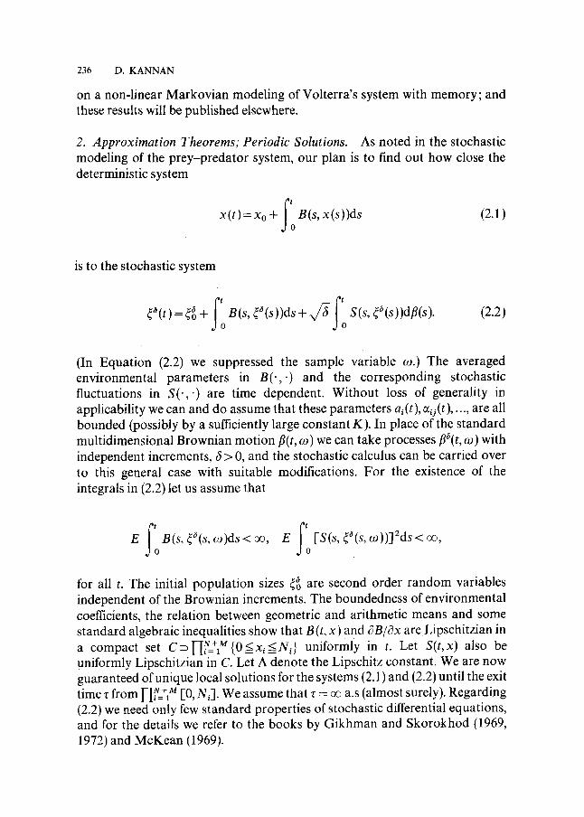
2. Approximation Theorems; Periodic Solutions. As noted in the stochastic modeling of the prey-predator system, our plan is to find out how close the deterministic system

I t

x(t) =Xo + B(s, x(s))ds dO

(2.1)

is to the stochastic system

f' f' ~(t) = ~ + B(s, ~(s))ds + x/~ S(s, ~(s))dfl(s). o o

(2.2)

(In Equation (2.2) we suppressed the sample variable o9.) The averaged environmental parameters in B(-,.) and the corresponding stochastic fluctuations in S( ' , ' ) are time dependent. Without loss of generality in applicability we can and do assume that these parameters ai(t), %(t),._, are all bounded (possibly by a sufficiently large constant K). In place of the standard multidimensional Brownian motion fl(t, o9) we can take processes fl6(t, o9) with independent increments, 6 > 0, and the stochastic calculus can be carried over to this general case with suitable modifications. For the existence of the integrals in (2.2) let us assume that

f' f' E B(s, ~6(s, o9)ds < ~ , E [S(s, ~6(s, og))]2ds < Z~, o o

for all t. The initial population sizes ~ are second order random variables independent of the Brownian increments. The boundedness of environmental coefficients, the relation between geometric and arithmetic means and some standard algebraic inequalities show that B(t, x) and •B/Ox areLiPschitzian in a compact s e t C~[-Ii~l=+lM{O~xi<_~Nit uniformly in t. Let S(t,x) also be uniformly Lipschitzian in C. Let A denote the Lipschitz constant. We are now guaranteed of unique local solutions for the systems (2.1) and (2.2) until the exit time z from I-I/s__+y [0, Ni]. We assume that z = ~ a.s (almost surely). Regarding (2,2) we need only few standard properties of stochastic differential equations, and for the details we refer to the books by Gikhman and Skorokhod (1969, 1972) and McKean (1969).

V O L T E R R A - V E R H U L S T PREY--PREDATOR SYSTEMS 237

In the absence of the Gaussian noises affecting the parameters, the stochastic equation (2.2) reduces to the deterministic equation (2.1). Noting that B(t,x) is the mean of B(t,~) and the mean of a stochastic integral E ~ b f (s, co)dfl(s, co) = 0, and taking the mathematical expectation on both sides of (2.2) we see that the deterministic system is equivalent in mean to the stochastic system (that is, the equivalence is in the L1 (f~) sense). It becomes necessary to find how close the higher moments of these systems are. This will assert, in a suitable sense, the closeness of the two systems. Towards this we begin with

THEOREM 2.1. /et m > l be an arbitrarily fixed integer, the non- anticipatory function S(t, o9) = S(t, r o9)) be such that E ~ ro S2"(t, og)dt < oo for all 0 < T< o% and the two systems begin with the same initial population size 30. Then

limE{ sup Ir og)-x(t)[ 2m} =0. (2.3) ,~.o 0 < t - < T

([ "1 is the usual N + M-dimensional norm.)

Proof. From (2.1) and (2.2)

E{0_<,_<Tsup I~(t, o9 ) -- x(t )l 2m }

<=(N+M)22mE [B(t,~6(t))-B(t,x(t))]dr o

{ ; } + (2a)'E sup l S(s,{a(s, o9))d~(s, o9)l 2m' O<t<=T 0

X ~(N+M)22mAm El~( t ,~ ) -x ( t , og)12mdt o

/ 4m 3 \m fT + (26) '{W---T/ r ' - i EIS(t, ~'(t))12mds

\ z m - l J o

_-<K1 o9)-x(t)[ dt o

238 D. KANNAN

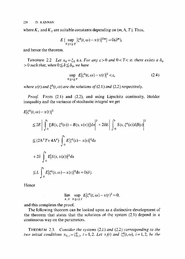
where K1 and Kz are suitable constants depending on (m, A, T). Thus,

E{ sup ]~6(t,r O<-t<-T

and hence the theorem.

THEOREM 2.2 Let x0 = 40 a.s. For any ~ > 0 and 0 < T< ~ there exists a 6o > 0 such that, when 0 < 6 <_ 6o, we have

sup El~6(t, r 2 < g , (2.4) O<t<_T

where x (t ) and ~6 (t, (~) a re the solutions of (2.1) and (2.2) respectively.

Proof From (2.1) and (2.2), and using Lipschitz continuity, Holder inequality and the variance of stochastic integral we get

el46(t, x(t)]

<=2E f : [B(s, ,6(S))-B(s,x(s))]ds2+26E

f )[ <(2A2T+4A 6) E ~(s)-x(s 2ds 0

+26 ElS(s,x(s))12ds 0

<=g 0

Hence

lim sup El~6(t,r 2=0, 6 1 . 0 0 < - t < T

and this completes the proof. The following theorem can be looked upon as a distinctive development of

the theorem that states that the solutions of the system (2.1) depend in a continuous way on the parameters.

THEOREM 2.3. Consider the systems (2.1) and (2.2) corresponding to the 6 two initial conditions Xo.i=~o.i, i--1,2. Let xi(t) and ~(t,m), i=1,2, be the

V O L T E R R A - V E R H U L S T PREY PREDATOR SYSTEMS 239

respective solutions. Then, for every e > 0 and 0 < T< 0% there is a 6o > 0 such that, when 0 < ~5 < 60, we have

sup E[~(t ,a))-Xx(t)-~2(t , oJ)+x2(t)lz<=eEIxo, x-Xo, z[ 2. (2.5) O<_t<_T

Proof In the following estimations we use the Lipschitz continuity of OB/Ox also. Bellman-Gronwall Lemma is repeatedly used. First

6 t I[~, ( , ") -- ~ (t, ',~)] [X, (t)-- X2(t)][ ~

2 f ' ) x2(s))]}ds 2 <= {[B(s ,~ ( s ) ) -B(s ,~ ( s ) ] - [B( s , x , ( s ) ) -B( s , o

2fi f t 2 + fs(~, ~ ( s ) ) - S(s, ~ ( s ) ) ] s ~ ( s ) . o

Next

[ B(s, ~ ( s ) ) - B(s, ~2 (s)) - B(s, xl (s)) + B(s, x2 (s))]ds

f, <_tE IB(s, ~ ( s ) ) -B(s , ~ ( s ) ) -B(s , xl(s))+B(s, x2(s))12ds o

<=2tE [B(s, x l (s ) ) -B(s , xz ( s ) ) -B(s ,~(s ) ) o

+ B(s, ~ (s) + x2 (s) - Xl (s))12ds

+2tE ]B(s, ~ ( s ) + x 2 ( s ) - x l ( s ) ) - B ( s , ~2(s))lZds o

<2ATE Ix,(s)-x2(s)l 2 I~(s,a))-x,(s)12ds o

+2A2tE [~(s,,.)-~2(s,o)-xx(s)+x2(s)I2ds o

<~K, EIx,(s)-x2(s)l 2 El~(s,'a))-x,(s)12ds o

240 D. K A N N A N

f, +K2 EJ~(s)-~(s)-xl(s)+x2(s)12ds o

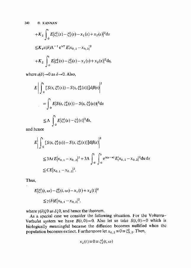
___KI~(~)A-, e AT ElXo. ~-Xo.212

f, o

where ~(6)~0 as 6 ~ 0 . Also,

El fto [S(s, ~ (s))- X(s, ~2(s))]d~(s)2

f = ElS(s, ~ ( s ) ) - S(s, Cg(s))12ds o

<=A E[~(s)-r o

and hence

t 2

f ; S 3 A t e [ X o . l - X o , ~ l ~ + 3A " e~-" 'E IXo .~ -Xo .~12d~ds o o

< CE[xo,, - Xo. 2[ ~.

Thus,

E[~ (t, co) - r (t, ~o) - x~ (t) + xz (0[ 2

_-<~(~)Elxo.,-Xo,2] ~,

where y(~)~0 as 6~0, and hence the theorem. As a special case we consider the following situation. For the Vo l t e r r a -

Verhulst system we have B( t ,0 )=0 . Also let us take S(t,O)=O which is biologically meaningful because the diffusion becomes nullified when the population becomes extinct. Fur thermore let Xo, 2 - 0 --- ~o, 2. Then,

xz(t)=-O=~z(t,~J))

VOLTERRA-VERHULST PREY--PREDATOR SYSTEMS 24i

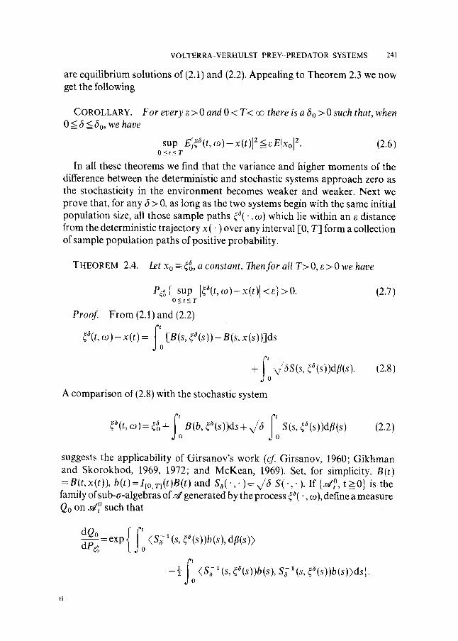
are equilibrium solutions of (2.1) and (2.2). Appealing to Theorem 2.3 we now get the following

COROLLARY. For every e > 0 and 0 < T< oo there is a 8o > 0 such that, when 0 <_ 8 <_ 80, we have

sup E[r 2 <eEIxo[ 2. (2.6) O<_t<_r

In all these theorems we find that the variance and higher moments of the difference between the deterministic and stochastic systems approach zero as the stochasticity in the environment becomes weaker and weaker. Next we prove that, for any 6 > O, as long as the two systems begin with the same initiaI population size, all those sample paths ~ ( . , ~) which lie within an e distance from the deterministic trajectory x ( ' ) over any interval [0, T] form a collection of sample population paths of positive probability.

THEOREM 2.4. let Xo -- ~o, a constant. Then for all T> O, e > 0 we have

Pr sup [~(t , t~)-x(t)]<e}>O. (2.7) O~t__<T

Proof From (2.1) and (2.2)

f ~~ (~))-x(t)= [B(s, ~O(s)) - B(s, x(s))]ds o

+ vieS(s, ~(s))dfl(s). (2.8) o

A comparison of (2.8) with the stochastic system

I t f ~(t, co)= ~o + B(b, ~ (s))ds + x/8 S(s, ~(s))dfl(s) d o o

(2.2)

suggests the applicability of Girsanov's work (cf Girsanov, 1960; Gikhman and Skorokhod, 1969, 1972; and McKean, 1969). Set, for simplicity, B(t) =B(t,x(t)), b(t)=IEo, Tl(t)B(t ) and S 6 ( ' , . ) = x / 6 S(- , . ) . If {N o , t>0} is the family of sub-a-algebras of s/generated by the process 40( �9 , ~o), define a measure Qo on sJ ~ such that

'f - 3 (S ; I ( s , ~O(s))b(s), S; i (s , ~(s))b(s))ds]. o

242 D. KANNAN

Then there exists a Brownian mot ion process fl*(t, co) such that

I t

~a(t, t o ) - x ( t ) = [B(s, ~6(s))-B(s, x(s))]ds o

St + x/6 S(s, ~6(s) )dfl*(s),

o

and Qo is equivalent to Pdo Girsanov, 1960). Now the result of Stroock (1971) on the growth of stochastic integrals applies, and hence

Qo{ sup O < t < . T

for all e > O. The equivalence of P~g and Qo implies that for all ~ > 0

P~{ sup [~6(t,,~)-x(t)[<e}>O. O<_t<=_T

This completes the proof. Staying with the spirit of limit theorems we pass to the stochastic system

(1.12) and deterministic system (1.13) and establish the said central limit property. After this we will return back to the systems (2.1) and (2.2) to discuss the stationary distributions and periodic solutions. Dropping the Gaussian noise fluctuation assumptions and taking general stochastic fluctuations we saw that the stochastic prey-preda tor system can be taken in the form

d ~v ~(t) = cS~(t, ~(t), r (2.9) ( I t

(see (1.12) and its derivation). As in the two previous systems (2.1) and (2.2) we can without loss of generality assume that the environmental parameters are bounded (and bounded below by a positive constant). Consider the N + M- dimensional vectors X such that 0 <Xi < R for a sufficiently large R > 0. Under these condit ions q~ is uniformly Lipschitz cont inuous in X if and only i fF is so. F rom now on we assume this Lipschitz continuity. Also let, for all t > 0 , P{qb(t, 0, co)=0) = 1. Now we have a unique local solution ~(t, cn) which is a cont inuous stochastic process. Let ZR be the hitting time of the boundary for the process ((t, to). By taking sufficiently large R we assume that -c R = 0o a.s. Fur thermore let the following ergodic type relation hold:

(2.9)

VOLTERRA-VERHULST PREY-PREDATOR SYSTEMS

as T~ oc. Set a slower time

243

Then,

z =6t and ~(z)=~(t)=~(z/fi).

d d~- 4o(z) =~(r/fi), ~(z/6), ~)

=~6(z, 46(r),,~), say.

Consider the following initial value problems

d -~(v)-----~o(z, ~a(z),~o), ~a(0)=40, (2.10) dt

d o o o ~ 4 (z)=~ (4 (z)), 4~ ~ (2.11)

Equation (2.10) denotes the stochastic system and (2.11) represents the averaged deterministic equations. These are the two systems we work with to establish the central limit property for the prey-predator system. More precisely it will be shown, under suitable conditions, that 6-1/2[~~ e)) - 4 ~ (t)] converges weakly to a diffusion process corresponding to a suitable N + M- dimensional Brownian motion. But first we state the

AVERAGING PROPERTY 2.5. Under the conditions with which we arrived at systems (2.10) and (2.11) we have

sup lEa(z, ~ ) - 4~ (2.12) 0-_<~<0(6 1)

as 6~0.

The proof of this averaging theorem is standard. Biogoljubov and Mitropolskii (1961) give a detailed account of this averaging principle in the deterministic case. Extensions of this principle to the stochastic case are now well known (see, for example, Hasminskii (1968), Kannan (1976) and Papanicolaou (1975).

The importance of central limit theorems,is well known. So it becomes fundamental to establish this central limit property for the stochastically evolving prey-predator system. Such theorems are basic in the theory of transport processes and Learning Theory, for example. Several methods for the convergence of (non-Markovian) processes to Gaussian Markov processes are

244 D. KANNAN

known (we refer to the recent expository article of Papanicalaou (1975) for an excellent account of this, and also see the references given there).) We adopt some of the s tandard steps to our case and minimize the details in the proof (see also Kannan, 1976).

Let {d~, 0 < s < t < t} be a family of sub-a-algebras of d such that (i) it is an increasing family: dT] ~ d ~ ifs < Sx < tl < t, and (ii) it satisfies the strong mixing condition: if u(co) and v(co) are any two r andom variables such that ued ~

lul < 1 and < l, then

sup sup [Euv - EuEv[ =f (z ),L O, (rT oQ ).

Define a process ~o(t, ~) by

(2.13)

(2.14)

The function F(t,X,~) arises as a stochastic fluctuation in the environment. Recall that the environmental parameters are assumed to be bounded. So, without much loss of generality we can and do assume that

r 0, r ~--~jr 3, ~:o) <K*,

02 (~) <K*, ~ ~ i ( t , ~ , i , j ,k=l ..... N+M. (2.15)

Also, let

and

lim E q?(t, ~)) = 0, (2.16) 6--+0

lim E[~ 6 (t, ~,)] 2 = 0.2 (t). (2.17)

The relations (2.16) and (2.17) will follow, under the strong mixing conditions, if

and

s 3o )-r176162 =o(6) Er ~, (s),~. (2.18)

(2.19)

VOLTERRA-VERHULST PREY PREDATOR SYSTEMS 245

on [0, To]. Here, 0"2(t) c a n be taken as ~ ak,({~ and

fTfT akl({ ) = lim T- 1 E[@k(S)--E~][~k(t)--Eggk]dS dt, T ~ a z 0 0

(2.20)

Next define the processes rla(t, to) and {a(t, r as follows:

and

E~~ co)=O, and E[~b~ (2.21)

,7"(t, , . )=a- laird(t, , . ) - (t)]

(a(t, tn) =0~(t, co)+ ~~176 ~O(s)ds. o

By the boundedness assumptions (2.15) and Bellman-Gronwall lemma, one gets

]~(t) I<(expK*t ~(t + ~(s ds . o

Hence the 2(N + M)-dimensional process (0~(t, t~), ~(t, c~)) is weakly compact in qf and the weak limit satisfies

J ~-~~176 ~~ (2.22)

With (lengthy) routine type of estimations one can show that

lim n{t/a(t, Cn)-~(t, Ca) @ 0} =0. (2.23)

where the limit is assumed to exist. Let cg =cg[0 ' To] be the space of continuous functions on [0, To] and #~ be the

measure on cg generated by the process Oo(t, a)), 6e(0, 6o]. Also let the mixing functionf(t) satisfy that ~;o tfl/3 (t)dt < oo. Now, from the definition of Oo(t, ~) and (2.18) and (2.19) it is easy to see that the family {pa, 6e (0, 6o]} is weakly compact (use Kolmogorov condition). Let po be the weak limit of {g0}, and O~ to) be the continuous process associated with po. Using characteristic functionals one can show that O~ to) is a Gaussian process with independent increments such that

246 D. KANNAN

But recall that ~~ ~) is a Gaussian process with independent increments with variance az(t). If SS* = [akl], then there is an (N + M)-dimensional Brownian motion process fl(t, so) such that d O~ ~) = S(4~ ~). Now from (2.22) and (2.23) it follows that

d r/~ (t, ~o)= I ~ O ~ (~~ ( t ) ) ]q~176 fl(t, t~).

Thus, we have established the following central limit property for a stochastically evolving prey-predator system.

THEOREM 2.6. Under the assumption (2.13), (2.15), (2.18), (2.19) and ~ tfl/a(t)dt < o~, the process qo(t,t~)=6-1/2[4a(t,t~)-r176 converges weakly to a diffusion process

d r/~ (t, ~n)=[ f~O ~ (40 (t))]q~ (t, ~:9)d t + S(~ ~ (t))dfl(t,~o),

where the diffusion coefficient is obtained from (2.20) and, 4 ~ and 4 ~ are the unique solutions of the stochastic prey-predator system (2.10) and deterministic averaged system (2.11 ) respectively.

Now we return back to the systems (2.1) and (2.2) and stay with them for the rest of this article. First we compare the equilibrium population levels of the deterministic and stochastic systems. Thus we work with the sets of stationary distributions of these systems. It is shown that the collection of weak limits of stationary distributions of stochastic systems ~a(t,~o) is a subcollection of stationary distributions of the deterministic system. Hence, if the deterministic prey-predator system has a unique equilibrium level, then every sequence of equilibrium levels of the stochastic system converges to that unique level. The diffusion processes ~ ( t ,~ ) are strong Markov processes. The deterministic evolution is also a Markovian system with transition probability Po (s, x; t, A) given by

P(x' y ; t' A )=fx~;s'Y)(A )={ 1'0, ifotherwise,X(t;s,y)~A

where x(t; s, y) is the solution x(t) with initial condition x(s) = y. So, in terms of Markov processes we are looking at stationary distributions, and would like to find the relation between stationary distributions of deterministic and stochastic evolutions.

Let K = HN+I M [0, Ri] where each R i = R, a sufficiently large real number,

VOLTERRA-VERHULST PREY--PREDATOR SYSTEMS 247

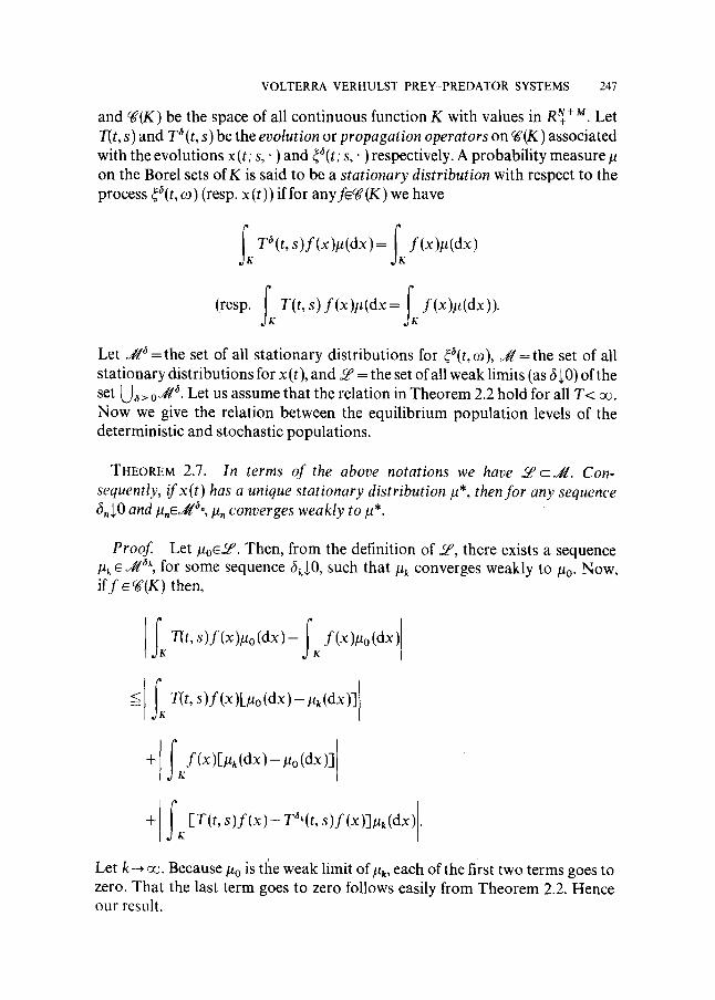
and Cg(K) be the space of all cont inuous function K with values in Ru+ +M. Let T(t, s) and T ~ (t, s) be the evolution or propagation operators on (g(K) associated with the evolutions x (t; s,. ) and in(t; s,. ) respectively. A probability measure # on the Borel sets of K is said to be a stationary distribution with respect to the process ~(t , co) (resp. x(t)) if for anyfe~(K) we have

fr To(t, s)f(x)la(dx) = f~ f(x)p(dx)

(resp. fK T(t,s) f(x)#(dx= fKf(x)#(dx)).

Let Jr162 = t h e set of all stationary distributions for r ~ = t h e set of all stationary distributions for x (t), and ~ = the set of all weak limits (as 6;0) of the set U~> o ~'~. Let us assume that the relation in Theorem 2.2 hold for all T< 0o. Now we give the relation between the equilibrium populat ion levels of the deterministic and stochastic populations.

THEOREM 2.7. In terms of the above notations we have ~ c ~ l . Con- sequently, if x(t) has a unique stationary distribution kt*, then for any sequence 6,J,O and #,E J r '~., #n converges weakly to I,t*.

Proof. Let #oe5 ~ Then, from the definition of LP, there exists a sequence #k 6 j/6k, for some sequence 6k.10 , such that #k converges weakly to/to. Now, i f f E ~(K) then,

If , Ttt, s)f(x)Szo(dx)-ff(x) o(dx)

< fK T(t, s)f(x)[#o(dx)-~tk(dX)]

+ f f (x)r,, (dx) - #o (dx)]

+ f r [T(t, s ) f ( x ) - T~*(t, s)f(x)]#k(dX).

Let k--, oo. Because/Zo is tt~e weak limit o f J/k, each of the first two terms goes to zero. That the last term goes to zero follows easily from Theorem 2.2. Hence our result.

248 D. KANNAN

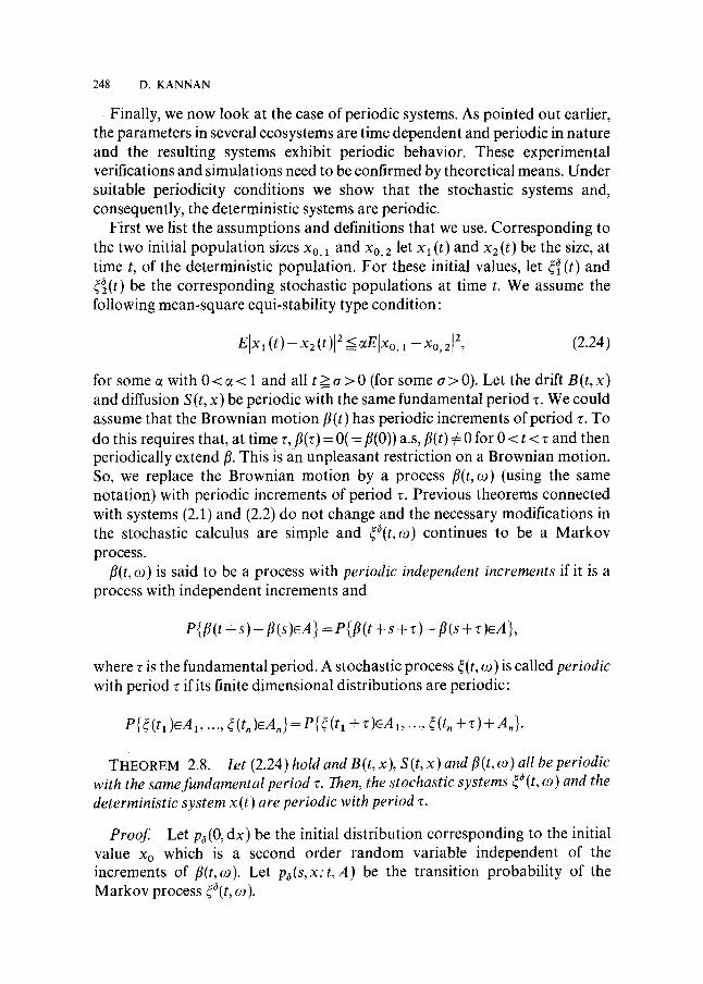
Finally, we now look at the case of periodic systems. As pointed out earlier, the parameters in several ecosystems are time dependent and periodic in nature and the resulting systems exhibit periodic behavior. These experimental verifications and simulations need to be confirmed by theoretical means. Under suitable periodicity condit ions we show that the stochastic systems and, consequently, the deterministic systems are periodic.

First we list the assumptions and definitions that we use. Corresponding to the two initial popula t ion sizes Xo, a and X0,z let xa (t) and Xz(t) be the size, at time t, of the deterministic populat ion. For these initial values, let ~] (t) and ~ ( t ) be the corresponding stochastic populat ions at t ime t. We assume the following mean-square equi-stability type condit ion:

E[X 1 (t)-- x2( t ) [ 2 <Z~Elxo, 1 -- Xo,2[ 2, (2.24)

for some a with 0 < a < 1 and all t > a > O (for some a > 0 ) . Let the drift B(t ,x) and diffusion S(t, x) be periodic with the same fundamental period z. We could assume that the Brownian mot ion fl(t) has periodic increments of period z. To do this requires that, at time z, fl(z) = 0( = fl(0)) a.s, fl(t) (: 0 for 0 < t < z and then periodically extend ft. This is an unpleasant restriction on a Brownian motion. So, we replace the Brownian mot ion by a process f l( t ,o) (using the same notat ion) with periodic increments of period ~. Previous theorems connected with systems (2.1) and (2.2) do not change and the necessary modifications in the stochastic calculus are simple and ~6(t,o~) continues to be a Markov process.

f l( t ,~) is said to be a process with periodic independent increments if it is a process with independent increments and

P{fl(t + s ) - fl(s)eA} = P{fl(t + s + ~ ) - fl(s + z)cA},

where r is the fundamental period. A stochastic process ~(t, ~o) is called periodic with period z if its finite dimensional distributions are periodic:

P{~(t, )eA1 ..... ~( t , )eA,}=P{~ (t, + z)eA,, ..., ~(t, + z) + A,}.

THEOREM 2.8. /e t (2.24) hold and B ( t, x ), S ( t, x) and fl ( t, co) all be periodic with the same fundamental period ~. Then, the stochastic systems ~a(t, ~ ) and the deterministic system x(t) are periodic with period ~.

Proof Let p~(0, dx) be the initial distribution corresponding to the initial value Xo which is a second order r andom variable independent of the increments of fl(t,~). Let p~(s,x;t ,A) be the transition probabili ty of the Markov process Co(t, ~).

V O L T E R R A - V E R H U L S T P R E Y - P R E D A T O R SYSTEMS 249

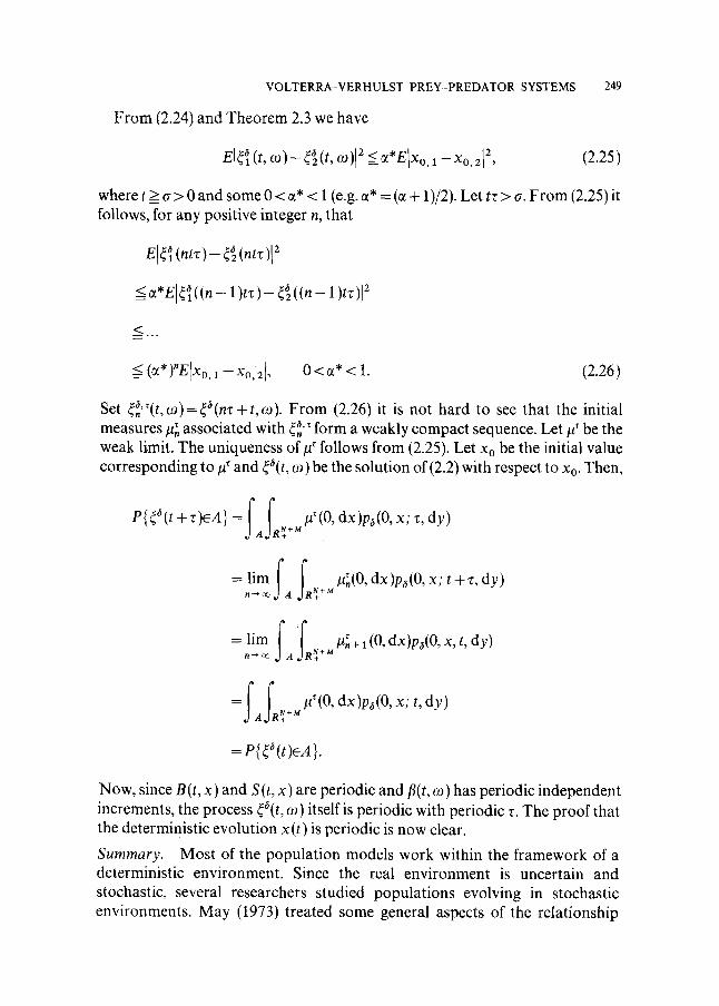
From (2.24) and Theorem 2.3 we have

=_ X 2 El{ { (t, o ) - r ,,)12 < ~*Elxo, 1 - 0,2[ , (2.25)

where t > o- > 0 and some 0 < e* < 1 (e.g. e* = (~ + 1)/2). Let tr > a. F rom (2.25) it follows, for any positive integer n, that

EIr ~ (ntr ) - ~ (ntT)l 2

<~*El~((n- 1) t z ) - ~2((n - 1)tr)] z

< (o~*)"EIxo, ~ - x0,2{, 0 < ~* < 1. (2.26)

Set {~.'~(t,o)={a(n~+t,o). From (2.26) it is not hard to see that the initial measures #~, associated with {~.'~ form a weakly compact sequence. Let #~ be the weak limit. The uniqueness of/~ follows from (2.25). Let x 0 be the initial value corresponding to #' and ~a(t, co) be the solution of (2.2) with respect to Xo. Then,

=limf. a la~"(O' dx)p~(O'x; t + r' dY)

= lim #,~ + t (0, dx)p~(O, x, t, dy) n ~ ~ A N++M

=f fRa ~++M/~(O'dx)pa(O'x;t'dy)

=P{~O(t)~A}.

Now, since B(t, x) and S(t, x) are periodic and fl(t, ~o) has periodic independent increments, the process ~(t, ~o) itself is periodic with periodic z. The proof that the deterministic evolution x(t) is periodic is now clear.

Summary. Most of the populat ion models work within the framework of a deterministic environment. Since the real environment is uncertain and stochastic, several researchers studied populations evolving in stochastic environments. May (1973) treated some general aspects of the relationship

250 D. KANNAN

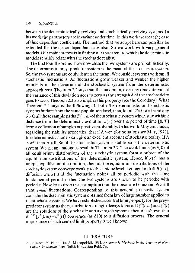
between the deterministically evolving and stochastically evolving systems. In his work the parameters are invariant under time. In this work we treat the case of time dependent coefficients. The method that we adopt here can possibly be extended for the space dependent case also. So we work with very general models. Our main interest is in finding out the extent to which the deterministic models sensibly relate with the stochastic reality.

The first four theorems show how close the two systems are probabilistically. The deterministic prey-predator system is the mean of the stochastic system. So, the two systems are equivalent in the mean. We consider systems with small stochastic fluctuations. As fluctuations grow weaker and weaker the higher moments of the deviation of the stochastic system from the deterministic approach zero. Theorem 2.2 says that the maximum, over any time interval, of the variance of this deviation goes to zero as the strength 6 of the stochasticity goes to zero. Theorem 2.3 also implies this property (see the Corollary). What Theorem 2.4 says is the following: If both the deterministic and stochastic systems initiate from the same population level, then, for all T> 0, e > 0 and any 6 > 0, all those sample paths ~ ( . , ~n) of the stochastic system which stay within distance from the deterministic evolution x(" ) over the period of time I-0, T] form a collection of samples of positive probability. In his work May concludes, regarding the stability properties, that if A > (7 z (for notations see May, 1973), the deterministic models can give an excellent account of stochastic reality. If A > ~z, then A > 0. So, if the stochastic system is stable, so is the deterministic system. We get an analogous result in Theorem 2.7. The weak limits (as 6+0) of all equilibrium distributions of the stochastic system form a subset of the equilibrium distributions of the deterministic system. Hence, if x(t) has a unique equilibrium distribution, then all the equilibrium distributions of the stochastic system converge weakly to this unique level. Let regular drift B(t, x ), diffusion S(t,x) and the fluctuation noises all be periodic with the same fundamental period ~, then the two systems are shown to be periodic with period ~. Now let us drop the assumption that the noises are Gaussian. We still treat small fluctuations. Corresponding to this general stochastic system consider the deterministic system obtained from law of large number applied to the stochastic system. We have established a central limit property for the prey- predator system as the perturbation strength decays to zero. If ~~ r and ~~ are the solutions of the stochastic and averaged systems, then it is shown that ~-1/2[~(t, C0)--~~ converges (as 6~0) to a diffusion process. The general importance of such central limit property is well known.

LITERATURE Bogoljubo~, N~ N. and Ju. A. Mitropolskii. 1961. Asymptotic Methods in the Theory of Non-

Linear Oscillation, New Delhi: Hindustan Publ. Co.

VOLTERRA VERHULST PREY--PREDATOR SYSTEMS 251

Gard, T. C. and D. Kannan. 1976. "On a Stochastic Differential Equation Modeling of Prey- Predator Evolution." J. Appl. Prob., 13.

Gikhman, I. I. and A. V. Skorokhod. 1969. Introduction to the Theory of Random Processes. Philadelphia: W. B. Saunders.

- - - - a n d - - . 1972. Stochastic Differential Equations. New York: Springer-Verlag. Girsanov, L V.. 1960. "On Transforming a Certain Class of Stochastic Processes by Absolutely

Continuous Substitution of Measures. Theory Prob. Appl., 5, 285-301. Hasminsk]i, R. Z. (Khasminskii). 1968. "On the Principle of Averaging for Ito's Stochastic

Differential Equations." Kybernetika (Prague), 4,260-279. (Russian). Kannan, D. 1976. "On some Markov Models of Certain Interacting Populations." Bull. Math.

Biol., 38, 723-738. - - - - . 1976. "Random Integrodifferential Equations," in Probabilistic Analysis and Related

Topics, (Ed. A. T. Bharucha-Reid). New York: Academic Press. - - - - . -Vot tarra ' s Prey-Predator Population With Historical Actions, in preparation. May, R. M. !973. Stability and Complexity in Model Ecosystems, Princeton, N.J.: Princeton

Univ. Press. �9 1974. "How Many Species: Some Mathematical Aspects of the Dynamics of

Populations" in Lectures on Mathematics in the Life Sciences, Vol. 6, pp. 65 98. Providence: AMS.

McKean, H. P. 1969. Stochastic Integrals. New York: Academic Press�9 Myers, J. H. and C. J. Krebs. 1974. "Population Cycles in Rodents," Scientific American, 230, 38-

46. Papanicolaoti, G. C. 1975. "Asymptotic Analysis of Transport Processes." Bull. Am. Math. Soc.,

81, 33(~392. Parthasarathy, K. R. 1967. Probability Measures on Metric Spaces. New York: Academic Press. Stroock, D. W. 1971. "On the Growth of Stochastic Integrals." Z. Wahrscheinlickeitstheorie, 18,

340-344. Wiegert, R. G., et al. 1975. "A Preliminary Ecosystem Model of Coastal Georgia Spartina

Marsh�9 Estuarine Research, 1,583-601.

RECEIVED 12-2-76