energies

Article

Voltage Distribution–Based Fault Location forHalf-Wavelength Transmission Line withLarge-Scale Wind Power Integration in China

Pulin Cao 1, Hongchun Shu 1,*, Bo Yang 1, Na An 1, Dalin Qiu 1, Weiye Teng 1 and Jun Dong 2

1 Faculty of Electric Power Engineering, Kunming University of Science and Technology, Kunming 650500,China; pulincao_kust@sina.com (P.C.); yangbo_ac@outlook.com (B.Y.); anna073000@163.com (N.A.);somesince2009@163.com (D.Q.); tengweiye@yeah.net (W.T.)

2 Harbin Institute of Technology, Harbin 150001, China; dongjun_kust@sina.com* Correspondence: kmshc@sina.com; Tel.: +86-137-088-47646

Received: 1 February 2018; Accepted: 1 March 2018; Published: 8 March 2018

Abstract: Large-scale wind farms are generally far away from load centers, hence there is anurgent need for a large-capacity power transmission scheme for extremely long distances, suchas half-wavelength transmission lines (HWTLs), which can usually span thousands of kilometersfrom large-scale wind farms to load centers. An accurate fault location method for HWTLs isneeded to ensure safe and reliable operation. This paper presents the design of a modal voltagedistribution–based asynchronous double-end fault location (MVD-ADFL) scheme, in which the phasevoltages and currents are transformed to modal components through a Karenbauer transformationmatrix. Then, the modal voltage distributions along transmission lines are calculated by voltage andcurrent from double ends. Moreover, the minimums and intersection points of calculated modalvoltages from double ends are defined as the fault location estimation. In order to identify incorrectfault location results and reduce calculation errors for the correct ones, air modal and earth modalvoltage distributions are applied in the fault location estimations. Simulation results verify theeffectiveness of the proposed approach under different fault resistances, distances, and types. Lastly,a real-time digital simulator (RTDS)–based hardware-in-the-loop (HIL) test is undertaken to validatethe feasibility of implementing the proposed approach.

Keywords: half-wavelength transmission line; asynchronous double-end fault location; large-scalewind power integration; modal voltage distribution; hardware-in-the-loop test

1. Introduction

Due to unprecedented worldwide population expansion and rapid economic growth in the pastdecade, an ever-increasing demand for electrical power is inevitable. Traditional fossil fuels, whichsupply more than one-quarter of global electricity power, are widely believed to be the main cause ofsevere global warming, and sustainable energy, such as wind, solar, biomass, tidal, and geothermal,has become a promising solution for continuous fossil fuel depletion [1–4]. Nowadays, the costof renewable energy power generation has decreased with the development of manufacturing andmaterials technology [5–7]. In China, the installed capacity of wind power was more than 168 GWin 2016, which was an increase of 13.8% over the previous year [8]. However, large-scale windfarms require strict climatic and geographic conditions, i.e., appropriate wind speed and annuallystable and consistently abundant winds [9]. In reality, such areas are often far away from theload centers [10]. The high-voltage direct current (HVDC) transmission system is believed to bea plausible method for bulk power transmission over long distances [11], but the extremely highcost of ultra-high voltage power electronic devices is the main obstacle to wide application of HVDC.

Energies 2018, 11, 593; doi:10.3390/en11030593 www.mdpi.com/journal/energies

Energies 2018, 11, 593 2 of 22

Furthermore, the distance between the large-scale wind farms and load centers in China is usuallythousands of kilometers [12], thus the half-wavelength transmission line (HWTL) without reactivepower compensation or intermediate substations has been considered as a promising alternative forlong-distance transmission of bulk renewable energy [13].

Although the concept of natural half-wavelength power transmission has been proposed since1939 [14], the overvoltage, power demands, and other technical problems in modern power systemsare very different from the past. Due to the constant fundamental frequency of 50 Hz or 60 Hz,the length of HWTL is fixed at about 3000 km or 2500 km [15], which restricts its practical application.Consequently, a compensation algorithm was proposed in [16] to transform a transmission line shorterthan half-wavelength to the tuned HWTL with lumped compensation circuit by inductance andcapacitance. In addition, ref. [17] analyzed the differences in overvoltage, voltage distribution, andcurrent distribution between tuned HWTL and natural HWTL. In order to reduce the differencesbetween natural HWTL and tuned HWTL, a lumped compensation circuit was divided into a seriesof sections and the effects of different sections were thoroughly compared in [18]. Moreover, ref. [19]attempted to generate high frequency from 180 Hz to 360 Hz to make half-wavelength lines suitablefor short-distance transmission, in which an AC-AC or AC-DC-AC conversion is required to transformhigh-frequency power to a 50 Hz or 60 Hz component for traditional fundamental frequency loads.

Generally speaking, HWTL can be adversely affected by extreme environmental conditions, e.g.,storms [20], lightning [21], forest fires [22], and ice shedding [23]; such conditions can significantlyreduce the air gaps between transmission lines or easily exceed the threshold of insulators, so thata breakdown of transmission line insulation might occur. For the purpose of quickly locatingthe fault point, several fault location algorithms have been proposed and developed over thepast decades, which can be generally classified into the following three groups: (a) fundamentalfrequency–based method [24], (b) transmission line differential equations [25], and (c) travellingwave method [26]. In particular, they are suitable for different fault types and causes. The firstone only needs a low-frequency sampling rate (around 6.4 kHz) but a long time window of voltageand current (>20 ms) [27]; the second one requires accurate transmission line impedance and ahigh-frequency sampling rate (around 10 kHz) of voltage and current [25]; the third one requires anultra-high-frequency sampling rate (>500 kHz) and a short time window (<5 ms) of current or voltage,in which the signal magnitude will be inevitably decayed in HWTL [28].

In fact, the above three approaches are all based on the following two techniques: (1) single-enddata–based fault location [29] and (2) double-end data–based fault location [30]. Normally, the faultlocation accuracy of the former can be considerably degraded as the distance of transmission lineincreases. Although the fault location accuracy of the latter is insensitive to transmission line distance,it requires accurate synchronous voltages and currents of double ends, which are hard to obtain inHWTL. To handle this challenge, this paper proposes a modal voltage distribution–based asynchronousdouble-end fault location (MVD-ADFL) method that does not require synchronous voltages andcurrents. It merely needs a low-frequency sampling rate (around 6.4 kHz) and a long time window ofvoltage and current (around 20 ms). At first, the modal voltages and currents are calculated from threeasynchronous phases by applying phase-modal transformation matrix. Then, the voltages distributedalong the modal circuit are calculated from double ends independently. Finally, the fault point ischosen from the interconnection points of modal voltages distributed along transmission lines or theminimum of particular air modal voltage distributions along transmission lines.

The rest of this paper is organized as follows: Section 2 is devoted to modelling of parallelmulticonductor transmission lines, and Section 3 develops the wavelength calculations of differentmodes in HWTL. Section 4 presents the design of the MVD-ADFL method for HWTL. In Section 5,simulation and real-time digital simulator (RTDS)–based hardware-in-the-loop (HIL) test results ondifferent fault types, distances, resistances, and wind generator capacities are presented to verify theeffectiveness of MVD-ADFL. Section 6 presents a discussion of the adaptivity of MVD-ADFL and the

Energies 2018, 11, 593 3 of 22

influence of generator types. Finally, some conclusions and possible future studies are summarized inSection 7.

2. Modelling of Parallel Multiconductor Transmission Lines

Three-phase transmission lines can be approximated by aggregating equivalent circuit segmentsdistributed along the lines. A line segment with length dx can be represented by an equivalent resistor,inductor and capacitor (RLC) circuit, as illustrated in Figure 1, in which the parameters of three linesare assumed to be identical in this paper.

Energies 2018, 11, x FOR PEER REVIEW 3 of 21

2. Modelling of Parallel Multiconductor Transmission Lines

Three-phase transmission lines can be approximated by aggregating equivalent circuit segments distributed along the lines. A line segment with length dx can be represented by an equivalent resistor, inductor and capacitor (RLC) circuit, as illustrated in Figure 1, in which the parameters of three lines are assumed to be identical in this paper.

′Ci

′Bi

Ai′

Figure 1. Equivalent RLC-based transmission line segment.

The equations of lossy three-phase transmission lines with constant parameters can be written as

A A B C0 A 0 B C

B B A C0 B 0 A C

C C A B0 C 0 A B

( 2 ) ( 2 ) ( ) ( )

( 2 ) ( 2 ) ( ) ( )

( 2 ) ( 2 ) ( ) ( )

i u u uG G u C C G u u Cx t t ti u u uG G u C C G u u Cx t t ti u u uG G u C C G u u Cx t t t

∂ ∂ ∂ ∂− = + + + − + − + ∂ ∂ ∂ ∂ ∂ ∂ ∂ ∂− = + + + − + − + ∂ ∂ ∂ ∂

∂ ∂ ∂ ∂− = + + + − + − + ∂ ∂ ∂ ∂

, (1)

CA A BA

CB B AB

C C A BC

( )

( )

( )

iu i iRi L Mx t t t

iu i iRi L Mx t t tu i i iRi L Mx t t t

∂∂ ∂ ∂− = + + + ∂ ∂ ∂ ∂∂∂ ∂ ∂− = + + + ∂ ∂ ∂ ∂

∂ ∂ ∂ ∂− = + + + ∂ ∂ ∂ ∂

, (2)

where uμ and iμ are the voltage and current of phase μ (μ = A, B, and C), respectively; G0 and C0 are the conductance and capacitance per unit (p.u.) length between line and earth, respectively; G, C, and M are the conductance, capacitance, and mutual inductance between line and line in p.u., respectively; and R and L are the line resistance and inductance in p.u., respectively.

If only one frequency component needs to be analyzed in voltage and current, the time-domain Equations (1) and (2) can be transformed to the following frequency-domain equation:

A0 A 0 A B C B C

B0 B 0 B A C A C

C0 C 0 C A B A B

d ( 2 ) ( 2 ) ( ) ( )dd ( 2 ) ( 2 ) ( ) ( )dd ( 2 ) ( 2 ) ( ) ( )d

ω ω

ω ω

ω ω

− = + + + − + − +

− = + + + − + − +

− = + + + − + − +

I G G U j C C U G U U j C U UxI G G U j C C U G U U j C U UxI G G U j C C U G U U j C U Ux

, (3)

Figure 1. Equivalent RLC-based transmission line segment.

The equations of lossy three-phase transmission lines with constant parameters can be written as− ∂iA

∂x = (G0 + 2G)uA + (C0 + 2C) ∂uA∂t − G(uB + uC)− C( ∂uB

∂t + ∂uC∂t )

− ∂iB∂x = (G0 + 2G)uB + (C0 + 2C) ∂uB

∂t − G(uA + uC)− C( ∂uA∂t + ∂uC

∂t )

− ∂iC∂x = (G0 + 2G)uC + (C0 + 2C) ∂uC

∂t − G(uA + uB)− C( ∂uA∂t + ∂uB

∂t )

, (1)

− ∂uA

∂x = RiA + L ∂iA∂t + M( ∂iB

∂t + ∂iC∂t )

− ∂uB∂x = RiB + L ∂iB

∂t + M( ∂iA∂t + ∂iC

∂t )

− ∂uC∂x = RiC + L ∂iC

∂t + M( ∂iA∂t + ∂iB

∂t )

, (2)

where uµ and iµ are the voltage and current of phase µ (µ = A, B, and C), respectively; G0 and C0 arethe conductance and capacitance per unit (p.u.) length between line and earth, respectively; G, C, andM are the conductance, capacitance, and mutual inductance between line and line in p.u., respectively;and R and L are the line resistance and inductance in p.u., respectively.

If only one frequency component needs to be analyzed in voltage and current, the time-domainEquations (1) and (2) can be transformed to the following frequency-domain equation:

−d_I A

dx = (G0 + 2G)_UA + jω(C0 + 2C)

_UA − G(

_UB +

_UC)− jωC(

_UB +

_UC)

−d_I B

dx = (G0 + 2G)_UB + jω(C0 + 2C)

_UB − G(

_UA +

_UC)− jωC(

_UA +

_UC)

−d_I C

dx = (G0 + 2G)_UC + jω(C0 + 2C)

_UC − G(

_UA +

_UB)− jωC(

_UA +

_UB)

, (3)

Energies 2018, 11, 593 4 of 22

−d

_UAdx = R

_I A + jωL

_I A + jωM(

_I B +

_I C)

−d_UBdx = R

_I B + jωL

_I B + jωM(

_I A +

_I C)

−d_UCdx = R

_I C + jωL

_I C + jωM(

_I A +

_I B)

, (4)

where the angular frequency ω = 2πf ;_Uµ and

_I µ are the voltage and current of phase µ in the

frequency domain, f is the fundamental frequency, and j is the imaginary unit. Equations (3) and (4)are the three-phase wave equations.

The wave equations can be obtained from Equations (3) and (4) as−d2_UA

dx2 = (R + jωL)d_I A

dx + jωM(d_I B

dx + d_I C

dx )

−d2_UBdx2 = (R + jωL)d

_I B

dx + jωM(d_I A

dx + d_I C

dx )

−d2_UCdx2 = (R + jωL)d

_I C

dx + jωM(d_I B

dx + d_I A

dx )

, (5)

−d2_I A

dx2 = (G0 + 2G + jωC0 + 2jωC)d_UAdx +−(G + jωC)(d

_UBdx + d

_UCdx )

−d2_I Bdx2 = (G0 + 2G + jωC0 + 2jωC)d

_UBdx +−(G + jωC)(d

_UAdx + d

_UCdx )

−d2_I Cdx2 = (G0 + 2G + jωC0 + 2jωC)d

_UCdx +−(G + jωC)(d

_UBdx + d

_UAdx )

, (6)

In order to reduce the complexity of the equation, phase A is taken as an example. The relationship

between d2_UAdx2 and

_UA, d2_I A

dx2 and_I A can be written as

d2_UAdx2 = (R + jωL)[(G0 + 2G + jωC0 + 2jωC)

_UA − (G + jωC)(

_UB +

_UC)]

+jωM[(G0 + G + jωC0 + jωC)(_UB +

_UC)− 2(G + jωC)

_UA]

=13[2(R + jωL− jωM)(G0 + 3G + jωC0 + 3jωC)

_UA + (R + jωL + 2jωM)(G0 + jωC0)

_UA

+(R + jωL + 2jωM)(G0 + jωC0)(_UB +

_UC)

−(R + jωL− jωM)(G0 + 3G + jωC0 + 3jωC)(_UB +

_UC)]

, (7)

d2_I Adx2 = (G0 + 2G + jωC0 + 2jωC)[(R + jωL)

_I A + jωM(

_I B +

_I C)]

−(G + jωC)[(R + jωL + jωM)(_I B +

_I C) + 2jωM

_I A]

=13[2(R + jωL− jωM)(G0 + 3G + jωC0 + 3jωC)

_I A + (R + jωL + 2jωM)(G0 + jωC0)

_I A

+(R + jωL + 2jωM)(G0 + jωC0)(_I B +

_I C)

−(R + jωL− jωM)(G0 + 3G + jωC0 + 3jωC)(_I B +

_I C)]

(8)

Equations (7) and (8) are both ordinary differential equations, thus their solutions can beobtained as

_UA =

23(A1e−γ1x + A2eγ1x) +

13(A3e−γ0x + A4eγ0x) +

13(A5e−γ1x + A6eγ1x) +

13(A7e−γ0x + A8eγ0x), (9)

_I A =

23(B1e−γ1x + B2eγ1x) +

13(B3e−γ0x + B4eγ0x) +

13(B5e−γ1x + B6eγ1x) +

13(B7e−γ0x + B8eγ0x), (10)

whereγ0 =

√(R + jωL + 2jωM)(G0 + jωC0), (11)

γ1 =√(R + jωL− jωM)(3G + G0 + 3jωC + jωC0), (12)

Energies 2018, 11, 593 5 of 22

A1 to A4 and B1 to B4 are calculated from phase A, while A5 to A8 and B5 to B8 are from phases Band C.

The voltage and current of the sending end are denoted as

Ps =

[Us

Is

]=

UAs

UBs

UCs

IAs

IBs

ICs

, (13)

The voltage and current after propagation along transmission lines with number of x can bewritten as

Px = TPs, (14)

where

Px =

[Ux

Ix

]=

UAx

UBx

UCx

IAx

IBx

ICx

, (15)

T =

23

H1 +13

H2 −13

H1 +13

H2 −13

H1 +13

H2 −2ZC0

3H3 −

ZC1

3H4

ZC0

3H3 −

ZC1

3H4

ZC0

3H3 −

ZC1

3H4

−13

H1 +13

H223

H1 +13

H2 −13

H1 +13

H2ZC0

3H3 −

ZC1

3H4 −2ZC0

3H3 −

ZC1

3H4

ZC0

3H3 −

ZC1

3H4

−13

H1 +13

H2 −13

H1 +13

H223

H1 +13

H2ZC0

3H3 −

ZC1

3H4

ZC0

3H3 −

ZC1

3H4 −2ZC0

3H3 −

ZC1

3H4

− 23ZC0

H3 −1

3ZC1H4

13ZC1

H3 −1

3ZC2H4

13ZC1

H3 −1

3ZC2H4

23

H1 +13

H2 −13

H1 +13

H2 −13

H1 +13

H2

13ZC1

H3 −1

3ZC2H4 − 2

3ZC0H3 −

13ZC1

H41

3ZC1H3 −

13ZC2

H4 −13

H1 +13

H223

H1 +13

H2 −13

H1 +13

H2

13ZC1

H3 −1

3ZC2H4

13ZC1

H3 −1

3ZC2H4 − 2

3ZC0H3 −

13ZC1

H4 −13

H1 +13

H2 −13

H1 +13

H223

H1 +13

H2

, (16)

H1 = cosh(γ0x), (17)

H2 = cosh(γ1x), (18)

H3 = sinh(γ0x), (19)

H4 = sinh(γ1x), (20)

where γ0 and γ1 are the propagation constants and ZC0 and ZC1 are characteristic impedances,as follows:

ZC0 =

√R + jωL + 2jωM

G0 + jωC0, (21)

ZC1(s) =

√R + jωL− jωM

3G + G0 + 3jωC + jωC0, (22)

As shown in Equations (6)–(22), the voltage and current propagated along any transmissionline will be affected by electromagnetic waves travelling along other parallel conductors due tothe coupling of electromagnetic fields. If the characteristics of multiconductor transmission linesare symmetric, the electromagnetic wave propagating along those lines can be represented by thesum of three-phase voltage and current, with two different propagation constants and two differentcharacteristic impedances. In order to simplify the analysis of travelling waves in multiconductortransmission lines, the impedance matrix and admittance matrix are transformed to diagonal matrices,of which each diagonal element denotes the impedance and admittance of an uncoupled circuit,

Energies 2018, 11, 593 6 of 22

and the phase voltage and phase current are transformed to modal voltage and modal current thatpropagate along the special uncoupled circuit. In particular, most of the uncoupled circuits, e.g., airmode, represent the circuit between conductors, while one of them is the circuit named “earth mode”between line and earth.

3. Wavelength Calculation of Different Modes in HWTL

3.1. Configuration of HWTL in China

The largest onshore wind farm in the world is located in Gangsu and Inner Mongolia in northernChina, while the load centers are concentrated in southeast coastal areas thousands of kilometersaway from. As a result, large amounts of electricity generated by the wind farm cannot be effectivelytransmitted to the load centers, which wastes a huge amount of wind power annually. On the otherhand, the coastal load centers frequently encounter load-peak shifting in summer due to powershortages. In order to solve the dilemma of wasted wind power and power shortages in different areas,bulk power transmission technology over long distances becomes a crucial task.

The 1000 kV alternating current (AC) transmission line was implemented and has been operatingas a demonstration project for ultra-high-voltage extra-long-distance transmission in China since2009. The large-scale wind farms in northern China are nearly 3000 km away from load centersin Guangdong, as schematically shown in Figure 2, which makes half-wavelength transmissiongeographically possible.

Energies 2018, 11, x FOR PEER REVIEW 6 of 21

C1

0 0

( )3 3

R j L j MZ sG G j C j C

ω ωω ω

+ −=+ + +

, (22)

As shown in Equations (6)–(22), the voltage and current propagated along any transmission line will be affected by electromagnetic waves travelling along other parallel conductors due to the coupling of electromagnetic fields. If the characteristics of multiconductor transmission lines are symmetric, the electromagnetic wave propagating along those lines can be represented by the sum of three-phase voltage and current, with two different propagation constants and two different characteristic impedances. In order to simplify the analysis of travelling waves in multiconductor transmission lines, the impedance matrix and admittance matrix are transformed to diagonal matrices, of which each diagonal element denotes the impedance and admittance of an uncoupled circuit, and the phase voltage and phase current are transformed to modal voltage and modal current that propagate along the special uncoupled circuit. In particular, most of the uncoupled circuits, e.g., air mode, represent the circuit between conductors, while one of them is the circuit named “earth mode” between line and earth.

3. Wavelength Calculation of Different Modes in HWTL

3.1. Configuration of HWTL in China

The largest onshore wind farm in the world is located in Gangsu and Inner Mongolia in northern China, while the load centers are concentrated in southeast coastal areas thousands of kilometers away from. As a result, large amounts of electricity generated by the wind farm cannot be effectively transmitted to the load centers, which wastes a huge amount of wind power annually. On the other hand, the coastal load centers frequently encounter load-peak shifting in summer due to power shortages. In order to solve the dilemma of wasted wind power and power shortages in different areas, bulk power transmission technology over long distances becomes a crucial task.

The 1000 kV alternating current (AC) transmission line was implemented and has been operating as a demonstration project for ultra-high-voltage extra-long-distance transmission in China since 2009. The large-scale wind farms in northern China are nearly 3000 km away from load centers in Guangdong, as schematically shown in Figure 2, which makes half-wavelength transmission geographically possible.

Figure 2. Geographical location of large-scale wind farm and load centers of China.

3.2. Wavelength Calculation of Ultra-High-Voltage HWTL

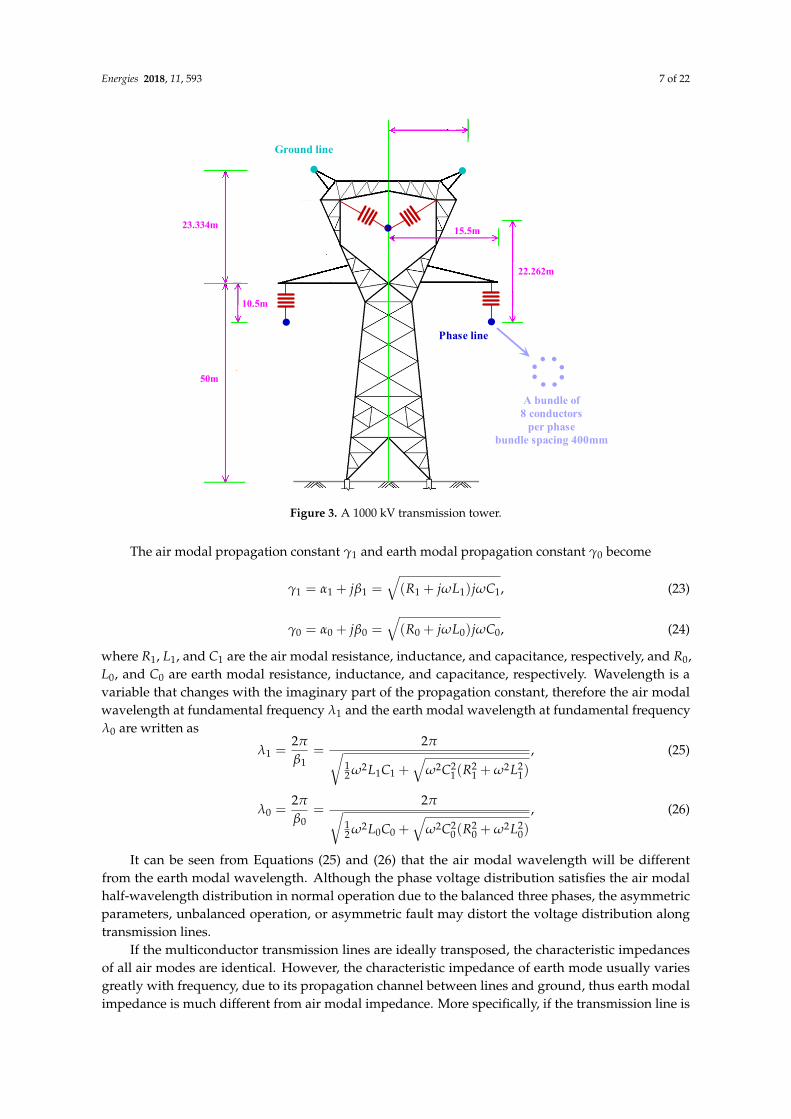
Due to the long distance, the half-wavelength transmission line needs a high-voltage level to reduce energy loss. Thus most research on half-wavelength is based on ultra-high-voltage, such as 1000 kV or higher. In this paper, the 1000 kV tower implemented in Jingdongnan-Nanyang-Jingmen is studied as demonstrated in Figure 3.

Figure 2. Geographical location of large-scale wind farm and load centers of China.

3.2. Wavelength Calculation of Ultra-High-Voltage HWTL

Due to the long distance, the half-wavelength transmission line needs a high-voltage level toreduce energy loss. Thus most research on half-wavelength is based on ultra-high-voltage, such as1000 kV or higher. In this paper, the 1000 kV tower implemented in Jingdongnan-Nanyang-Jingmen isstudied as demonstrated in Figure 3.

Energies 2018, 11, 593 7 of 22Energies 2018, 11, x FOR PEER REVIEW 7 of 21

Phase line

Ground line

A bundle of8 conductors

per phasebundle spacing 400mm

50m

10.5m

23.334m 15.5m

22.262m

Figure 3. A 1000 kV transmission tower.

The air modal propagation constant γ1 and earth modal propagation constant γ0 become

1 1 1 1 1 1( )j R j L j Cγ α β ω ω= + = + , (23)

0 0 0 0 0 0( )j R j L j Cγ α β ω ω= + = + , (24)

where R1, L1, and C1 are the air modal resistance, inductance, and capacitance, respectively, and R0, L0, and C0 are earth modal resistance, inductance, and capacitance, respectively. Wavelength is a variable that changes with the imaginary part of the propagation constant, therefore the air modal wavelength at fundamental frequency λ1 and the earth modal wavelength at fundamental frequency λ0 are written as

12 2 2 2 2 21

1 1 1 1 1

2 21 ( )2

LC C R L

π πλβ ω ω ω

= =+ +

, (25)

02 2 2 2 2 20

0 0 0 0 0

2 21 ( )2

L C C R L

π πλβ ω ω ω

= =+ +

, (26)

It can be seen from Equations (25) and (26) that the air modal wavelength will be different from the earth modal wavelength. Although the phase voltage distribution satisfies the air modal half-wavelength distribution in normal operation due to the balanced three phases, the asymmetric parameters, unbalanced operation, or asymmetric fault may distort the voltage distribution along transmission lines.

If the multiconductor transmission lines are ideally transposed, the characteristic impedances of all air modes are identical. However, the characteristic impedance of earth mode usually varies greatly with frequency, due to its propagation channel between lines and ground, thus earth modal impedance is much different from air modal impedance. More specifically, if the transmission line is short, the voltage distribution along that line and the different modal characteristics have no

Figure 3. A 1000 kV transmission tower.

The air modal propagation constant γ1 and earth modal propagation constant γ0 become

γ1 = α1 + jβ1 =√(R1 + jωL1)jωC1, (23)

γ0 = α0 + jβ0 =√(R0 + jωL0)jωC0, (24)

where R1, L1, and C1 are the air modal resistance, inductance, and capacitance, respectively, and R0,L0, and C0 are earth modal resistance, inductance, and capacitance, respectively. Wavelength is avariable that changes with the imaginary part of the propagation constant, therefore the air modalwavelength at fundamental frequency λ1 and the earth modal wavelength at fundamental frequencyλ0 are written as

λ1 =2π

β1=

2π√12 ω2L1C1 +

√ω2C2

1(R21 + ω2L2

1)

, (25)

λ0 =2π

β0=

2π√12 ω2L0C0 +

√ω2C2

0(R20 + ω2L2

0)

, (26)

It can be seen from Equations (25) and (26) that the air modal wavelength will be differentfrom the earth modal wavelength. Although the phase voltage distribution satisfies the air modalhalf-wavelength distribution in normal operation due to the balanced three phases, the asymmetricparameters, unbalanced operation, or asymmetric fault may distort the voltage distribution alongtransmission lines.

If the multiconductor transmission lines are ideally transposed, the characteristic impedancesof all air modes are identical. However, the characteristic impedance of earth mode usually variesgreatly with frequency, due to its propagation channel between lines and ground, thus earth modalimpedance is much different from air modal impedance. More specifically, if the transmission line is

Energies 2018, 11, 593 8 of 22

short, the voltage distribution along that line and the different modal characteristics have no significantinfluence on line protection or overvoltage, but the half-wavelength line is too long to ignore theinfluence of different wavelength of modes.

4. Modal Voltage Distribution–Based Asynchronous Double-End Fault Location

4.1. Phase-Modal Transformation

Considering the different characteristics of air mode and earth mode, the phase current andvoltage can be transformed into modal components by the Karenbauer transform matrix [31] as

_Uα_Uβ_Uχ_U0

=

1 −1 01 0 −10 1 −11 1 1

_UA_UB_UC

, (27)

A two-port network is used to represent the ideally transposed line by _Uϕx_I ϕx

=

cosh(γϕx) −Zcϕsinh(γϕx)

− 1Zcϕ

sinh(γϕx) cosh(γϕx)

_Uϕs_I ϕs

, (28)

where ϕ = 0, α, β and χ. Uϕs and Iϕs are the sending end voltage and current, respectively; Uϕx and Iϕx

are voltage and current away from sending end with distance x, respectively; γα, γβ, and γχ are allequal to γ1; and Zcα, Zcβ, and Zcχ are all equal to Zc1. The modes α, β, and χ are all air modes withdifferent circuits, while their characteristics are almost the same if the transmission lines are ideallytransposed. On the other hand, the voltage distributed along transmission lines can also be obtainedby the voltage and current of the receiving end, as follows: _

Uϕlx_I ϕlx

=

cosh(γϕ(l − x)) Zcϕsinh(γϕ(l − x))1

Zcϕsinh(γϕ(l − x)) cosh(γϕ(l − x))

_Uϕr_I ϕr

, (29)

where Uϕlr and Iϕlr represent the voltage and current of receiving end, respectively, and l is the totallength of faulty line. Here, each point in the ideally transposed line has the same voltage, calculated byEquations (28) and (29), but the fault point is a boundary of ideally transposed line, which makes thereal voltage different from the calculated voltage. Since the transform matrix cannot decouple the faultpoint resulting from the three-phase unbalance at the fault point, the actual voltage and the calculatedvoltage are quite different in the region between the fault point and the remote end.

4.2. Fault Location of Phase-to-Ground Fault

The fault point separates the line into two sections, in which the actual voltage is similar to thecalculated voltage at the near end but much different at the remote end. Hence, the calculated voltagefrom each end may obtain the same value at fault point but much different values at other points.The fault distance can be written as

x =1

γφtanh−1

Zcφ

_I rφsinh(γφl)−

_Urφ cosh(γφl) +

_Usφ

Zcφ

_I rφ cosh(γφl)−

_Urφsinh(γφl) + Zcφ

_I sφ

, (30)

where x could be a complex number with a small imaginary part due to the numerical calculationerror, thus the fault distance can be written as

Energies 2018, 11, 593 9 of 22

x =

∣∣∣∣∣∣ 1γφ

tanh−1

Zcφ

_I rφsinh(γφl)−

_Urφ cosh(γφl) +

_Usφ

Zcφ

_I rφ cosh(γφl)−

_Urφsinh(γφl) + Zcφ

_I sφ

∣∣∣∣∣∣, (31)

where l is the line length. Equation (31) needs synchronized measurements from both ends.However, numerous factors, such as thunderstorms and electromagnetic interference, will degrade thesynchronization accuracy. The fault location method with unsynchronized data from both ends shallbe discussed.

The angle of fundamental frequency voltage and current are time-varying, but their amplitude isstable when the fault transients are attenuated. Considering the voltage amplitude, Equation (30) canbe rewritten as∣∣∣∣Zcφ

_I rφsinh(γφl) cosh(γφx)−

_Urφ cosh(γφl) cosh(γφx) +

_Usφ cosh(γφx)

∣∣∣∣=

∣∣∣∣Zcφ

_I rφ cosh(γφl)sinh(γφx)−

_Urφsinh(γφl)sinh(γφx) + Zcφ

_I sφsinh(γφx)

∣∣∣∣ , (32)

If the transmission lines are ideally transposed, the characteristic impedances of all air modesare almost the same. Thus, only the air modal circuit containing the faulty phase line is selected tocalculate the voltage distribution. Thus, Equation (32) becomes∣∣∣∣Zc1

_I r1sinh(γ1l) cosh(γ1x)−

_Ur1 cosh(γ1l) cosh(γ1x) +

_Us1 cosh(γ1x)

∣∣∣∣=

∣∣∣∣Zc1_I r1 cosh(γ1l)sinh(γ1x)−

_Ur1sinh(γ1l)sinh(γ1x) + Zc1

_I s1sinh(γ1x)

∣∣∣∣ , (33a)

∣∣∣∣Zc0_I r0sinh(γ0l) cosh(γ0x)−

_Ur0 cosh(γ0l) cosh(γ0x) +

_Us0 cosh(γ0x)

∣∣∣∣=

∣∣∣∣Zc0_I r0 cosh(γ0l)sinh(γ0x)−

_Ur0sinh(γ0l)sinh(γ0x) + Zc0

_I s0sinh(γ0x)

∣∣∣∣ , (33b)

Here, the calculated voltage distribution along transmission lines between the fault point and theremote end are quite different from the real voltage distribution. However, it may obtain intersectionpoints with calculated voltage from another end casually. As a result, Equations (33a) and (33b) mightcontain multiple solutions, while additional conditions should be taken into account to accomplishan accurate fault location. Moreover, Equations (33a) and (33b) always have the similar fault locationestimation near the fault point, and the characteristics of different modes lead to different periods ofvoltage distribution along transmission lines, so inaccurate fault location estimations can be eliminatedby the significant difference between the air mode and earth estimations. Denoting the air mode faultlocation estimation as x1 and the earth mode fault location estimation as x0, the following inequalityneeds to be satisfied:

|x1 − x0|≤ η, (34)

where η is the threshold between x1 and x0, and η is set as 5% × 3000 km = 150 km in this paper.The calculation error and non-ideal models may lead to some differences between fault location

estimation of air mode and earth mode, while their mean value is used for an accurate fault locationresult xf1 as

xf1 =x1 + x0

2(35)

4.3. Fault Location of Phase-to-Phase Fault

If the transmission line fault is a phase-to-phase fault, where the fault point is still insulated toground, the earth modal voltage will equal zero. Hence, a fault location scheme without zero modalvoltage has to be considered.

Energies 2018, 11, 593 10 of 22

The modal voltage transformed by the phase-modal transformation matrix in Equation (27) canbe regarded as the voltage in an independent two-conductor modal circuit formed by two phase lines.If two faulty phase lines are applied to form the air modal circuit, the voltage of the fault point willbe the minimum. Therefore, the minimum of the calculated voltage along transmission lines can becalculated from double ends to locate the fault point of phase-to-phase fault. The fault location can berepresented as

_Uminr(xr) = min

∣∣∣∣Zc1_I r1sinh(γ1l) cosh(γ1x)−

_Ur1 cosh(γ1l) cosh(γ1x)

∣∣∣∣, (36a)

_Umins(xs) = min

∣∣∣∣Zc1_I s1sinh(γ1l) cosh(γ1x)−

_Us1 cosh(γ1l) cosh(γ1x)

∣∣∣∣, (36b)

Ideally, the minimum voltage distribution along transmission lines calculated by Equations (36a)and (36b) from double ends should be similar, and the next local minimum should be one-half airmodal wavelength away, such that the fault point can be treated as the global minimum in almostall faults. In addition, the calculation error increases as the distance grows, hence most of the faultlocation is more reliable in dealing with near-end fault. The calculated distance of the fault point canbe used as the weight ωr for receiving-end fault location estimation xr, and weight ωs for sending-endfault location estimation xs, which gives fault location result xf2 as

xf2 = ωrxr + ωsxs, (37)

where ωr =

xr

l

ωs =l − xs

l

, (38)

4.4. Overall Fault Location Scheme

If the methods in Sections 4.2 and 4.3 are applied for a fault, the final fault location result xf can bewritten as

xf =xf1 + xf2

2, (39)

To this end, the overall fault location scheme can be summarized in the following three procedures:

(1) Determine the faulty phase and fault type by reference [13] with a low-frequency sampling rate.(2) Apply transform matrix to obtain modal voltage and modal current, and choose an appropriate

modal circuit containing double faulty phases for voltage distribution calculation andfault location.

(3) If the fault type includes a ground fault, apply the intersection points of different modal voltagedistributions to locate the fault distance. Otherwise, the fault distance will be located by bothintersection points and minimum.

The overall flowchart of MVD-ADFL is demonstrated in Figure 4.

Energies 2018, 11, 593 11 of 22

Energies 2018, 11, x FOR PEER REVIEW 11 of 21

Figure 4. Overall flowchart of the modal voltage distribution based asynchronous double-end fault location (MVD-ADFL) method.

5. Case Studies

5.1. Simulation Model

A schematic diagram of the simulation model is depicted in Figure 5, while the tower shown in Figure 3 is used to calculate the transmission line parameters. Two hundred doubly fed induction generators [32] with 3 MW rated power and 25 m/s rated wind speed were considered for the wind farm, and were aggregated into an equivalent 600 MW generator in the model. The tower shown in Figure 3 was used to calculate the transmission line parameters. Bus M and bus N represent the sending and receiving end of transmission lines, respectively.

Figure 5. Schematic diagram of the simulation model.

Figure 4. Overall flowchart of the modal voltage distribution based asynchronous double-end faultlocation (MVD-ADFL) method.

5. Case Studies

5.1. Simulation Model

A schematic diagram of the simulation model is depicted in Figure 5, while the tower shown inFigure 3 is used to calculate the transmission line parameters. Two hundred doubly fed inductiongenerators [32] with 3 MW rated power and 25 m/s rated wind speed were considered for the windfarm, and were aggregated into an equivalent 600 MW generator in the model. The tower shownin Figure 3 was used to calculate the transmission line parameters. Bus M and bus N represent thesending and receiving end of transmission lines, respectively.

Energies 2018, 11, x FOR PEER REVIEW 11 of 21

Figure 4. Overall flowchart of the modal voltage distribution based asynchronous double-end fault location (MVD-ADFL) method.

5. Case Studies

5.1. Simulation Model

A schematic diagram of the simulation model is depicted in Figure 5, while the tower shown in Figure 3 is used to calculate the transmission line parameters. Two hundred doubly fed induction generators [32] with 3 MW rated power and 25 m/s rated wind speed were considered for the wind farm, and were aggregated into an equivalent 600 MW generator in the model. The tower shown in Figure 3 was used to calculate the transmission line parameters. Bus M and bus N represent the sending and receiving end of transmission lines, respectively.

Figure 5. Schematic diagram of the simulation model. Figure 5. Schematic diagram of the simulation model.

Energies 2018, 11, 593 12 of 22

Power Systems Computer Aided Design/Electromagnetic Transients including DC (PSCAD/EMTDC),an electromagnetic time-domain transient simulation environment created by Manitoba HydroInternational with a library of preprogrammed models and a design editor for building custommodels to satisfy various levels of different modelling demands, was adopted to construct a simulationmodel of HWTL with large-scale wind power integration; version 4.5 was used in this study [33–37].The simulation tests were implemented based on the PSCAD/EMTDC model, a general-purposetime-domain simulation tool for studying transient behavior of electrical networks. A single linediagram of the simulation model is provided in Figure 6, and its parameters are given in Tables 1–3.

Energies 2018, 11, x FOR PEER REVIEW 12 of 21

Power Systems Computer Aided Design/Electromagnetic Transients including DC (PSCAD/EMTDC), an electromagnetic time-domain transient simulation environment created by Manitoba Hydro International with a library of preprogrammed models and a design editor for building custom models to satisfy various levels of different modelling demands, was adopted to construct a simulation model of HWTL with large-scale wind power integration; version 4.5 was used in this study [33–37]. The simulation tests were implemented based on the PSCAD/EMTDC model, a general-purpose time-domain simulation tool for studying transient behavior of electrical networks. A single line diagram of the simulation model is provided in Figure 6, and its parameters are given in Tables 1–3.

Figure 6. Single line diagram of the simulation model in PSCAD.

Table 1. Parameters of the transformer at bus M.

Transformer MVA 1000.0 MVA Base Operation Frequency 50 Hz

Leakage Reactance 0.1 p.u. High-Voltage (HV) Winding Voltage 1100 kVLow-Voltage (LV) Winding Voltage 500 kV

Table 2. Parameters of the transformer at bus N.

Transformer MVA 1000.0 MVA Base Operation Frequency 50 Hz

Leakage Reactance 0.1 p.u. HV Winding Voltage 1000 kV LV Winding Voltage 550 kV

Table 3. Parameters of the wind turbine.

Generator Rate MVA 3 MVARated Wind Speed 12 m/s

Air Density 1.225 kg/m3 Resistance of Stator Winding 0.005 p.u.

Resistance of Rotator Winding 0.0055 p.u. Leakage Inductance of Stator Winding 0.4 p.u. Leakage Inductance of Stator Winding 0.44 p.u.

The frequency-dependent model was employed to represent transmission lines in the simulation. Table 4 shows the frequency-dependent parameters of transmission line when the fundamental frequency is 50 Hz, based on the tower shown in Figure 3 [38].

Figure 6. Single line diagram of the simulation model in PSCAD.

Table 1. Parameters of the transformer at bus M.

Transformer MVA 1000.0 MVABase Operation Frequency 50 Hz

Leakage Reactance 0.1 p.u.High-Voltage (HV) Winding Voltage 1100 kVLow-Voltage (LV) Winding Voltage 500 kV

Table 2. Parameters of the transformer at bus N.

Transformer MVA 1000.0 MVABase Operation Frequency 50 Hz

Leakage Reactance 0.1 p.u.HV Winding Voltage 1000 kVLV Winding Voltage 550 kV

Table 3. Parameters of the wind turbine.

Generator Rate MVA 3 MVARated Wind Speed 12 m/s

Air Density 1.225 kg/m3Resistance of Stator Winding 0.005 p.u.

Resistance of Rotator Winding 0.0055 p.u.Leakage Inductance of Stator Winding 0.4 p.u.Leakage Inductance of Stator Winding 0.44 p.u.

The frequency-dependent model was employed to represent transmission lines in the simulation.Table 4 shows the frequency-dependent parameters of transmission line when the fundamentalfrequency is 50 Hz, based on the tower shown in Figure 3 [38].

Energies 2018, 11, 593 13 of 22

Table 4. Parameters of different modes.

Mode Resistance (Ω/m) Inductance (H/m) Capacitance (F/m) Wavelength (m)

Air mode R1 = 1.032 × 10−5 L1 = 8.404 × 10−7 C1 = 1.375 × 10−11 λ1 = 5.882 × 106

Earth mode R0 = 2.513 × 10−4 L0 = 2.692 × 10−6 C0 = 8.804 × 10−12 λ0 = 4.065 × 106

It can be seen in Table 4 that the air mode wavelength is much larger than earth mode due to thedifferences between air modal circuit and earth modal circuit, hence the open-phase operation andunbalanced ground fault can induce quite different voltage distributions in air modal circuit and earthmodal circuit.

Normally, wind farms are required to achieve maximum power point tracking to track the optimalactive power curve, which is obtained by connecting each maximum power point at various windspeeds with the optimal active power curve determined by

Popt(ωm) = K∗ω3m, (40)

where K∗ = 0.5ρπR5C∗P/(λ∗)3 denotes the shape coefficient of optimal active power, R is the bladeradius of the wind turbine, ρ is the air density, the optimal tip-speed ratio λ∗ = 7.4, and the maximumpower coefficient C∗P = 0.4019 [33].

Hence, the power generated from the wind farm usually has a highly stochastic pattern, whichwill be injected into the main power grid [31]. Figure 7a,b demonstrate the wind speed and producedactive power of the wind farm, respectively.

Energies 2018, 11, x FOR PEER REVIEW 13 of 21

Table 4. Parameters of different modes.

Mode Resistance (Ω/m) Inductance (H/m) Capacitance (F/m) Wavelength (m) Air mode R1 = 1.032 × 10−5 L1 = 8.404 × 10−7 C1 = 1.375 × 10−11 λ1 = 5.882 × 106

Earth mode R0 = 2.513 × 10−4 L0 = 2.692 × 10−6 C0 = 8.804 × 10−12 λ0 = 4.065 × 106

It can be seen in Table 4 that the air mode wavelength is much larger than earth mode due to the differences between air modal circuit and earth modal circuit, hence the open-phase operation and unbalanced ground fault can induce quite different voltage distributions in air modal circuit and earth modal circuit.

Normally, wind farms are required to achieve maximum power point tracking to track the optimal active power curve, which is obtained by connecting each maximum power point at various wind speeds with the optimal active power curve determined by

* 3opt m m=P Kω ω（ ） , (40)

where * 5 * * 3p0.5 / ( )K R Cρπ λ= denotes the shape coefficient of optimal active power, R is the blade

radius of the wind turbine, ρ is the air density, the optimal tip-speed ratio * 7.4λ = , and the maximum power coefficient *

p 0.4019C = [33]. Hence, the power generated from the wind farm usually has a highly stochastic pattern, which

will be injected into the main power grid [31]. Figure 7a,b demonstrate the wind speed and produced active power of the wind farm, respectively.

(a) Wind speed (b) Produced active power

Figure 7. Wind speed and produced active power of the wind farm.

The hardware-in-the-loop (HIL) test is a powerful and important technique that has been used worldwide in real-time experiments instead of practical experiments due to the complexity and large scale of real power systems. The Real-Time Digital Simulator (RTDS), which is capable of closed-loop testing of protection and control equipment, was adopted in this study to further validate the feasibility of hardware implementation. The configuration and experimental platform of HIL test are provided in Figures 8 and 9.

Figure 7. Wind speed and produced active power of the wind farm.

The hardware-in-the-loop (HIL) test is a powerful and important technique that has been usedworldwide in real-time experiments instead of practical experiments due to the complexity and largescale of real power systems. The Real-Time Digital Simulator (RTDS), which is capable of closed-looptesting of protection and control equipment, was adopted in this study to further validate the feasibilityof hardware implementation. The configuration and experimental platform of HIL test are provided inFigures 8 and 9.

Energies 2018, 11, 593 14 of 22

Energies 2018, 11, x FOR PEER REVIEW 14 of 21

Figure 8. Configuration of the hardware-in-the-loop (HIL) test.

Figure 9. Experimental platform of the HIL test.

A power system with a sampling rate of 20 kHz was implemented by #16 RTDS with four PB5 processor cards and one gigabit transceiver analog output card, which can output the voltage and current at bus M and bus N. Meanwhile, #17 RTDS with three PB5 processor cards and one gigabit transceiver analog input card was applied as an acquisition device with 10 kHz to acquire voltage and current output from #16 RTDS. The voltage and current acquired by #17 RTDS was transferred to digital data and stored in RTDS as Common format for Transient Data Exchange (COMTRADE) 1999 files, which were then transmitted to a PC with an IntelR Core™ i3 CPU at 2.52 GHz and 3 GB of RAM. Finally, the voltage and current waveforms were decoded from COMTRADE 1999 files in the PC to locate fault points by the proposed MVD-ADFL.

Denoting the fault distance as xfault, the relative fault location calculation error ε is defined as

f fault| | 100%ε −= ×x xl

, (41)

where l is the total length of fault line and xf is the fault location result.

5.2. Single Phase-to-Ground Fault

A phase-to-ground (AG) fault with 200 Ω fault resistance, 2400 km away from bus M, which occurred at 10 s with a total wind power of 180 MW, was investigated by simulation and HIL test. The calculated voltage distribution along transmission lines from bus M and bus N are shown in Figure 10.

Figure 8. Configuration of the hardware-in-the-loop (HIL) test.

Energies 2018, 11, x FOR PEER REVIEW 14 of 21

Figure 8. Configuration of the hardware-in-the-loop (HIL) test.

Figure 9. Experimental platform of the HIL test.

A power system with a sampling rate of 20 kHz was implemented by #16 RTDS with four PB5 processor cards and one gigabit transceiver analog output card, which can output the voltage and current at bus M and bus N. Meanwhile, #17 RTDS with three PB5 processor cards and one gigabit transceiver analog input card was applied as an acquisition device with 10 kHz to acquire voltage and current output from #16 RTDS. The voltage and current acquired by #17 RTDS was transferred to digital data and stored in RTDS as Common format for Transient Data Exchange (COMTRADE) 1999 files, which were then transmitted to a PC with an IntelR Core™ i3 CPU at 2.52 GHz and 3 GB of RAM. Finally, the voltage and current waveforms were decoded from COMTRADE 1999 files in the PC to locate fault points by the proposed MVD-ADFL.

Denoting the fault distance as xfault, the relative fault location calculation error ε is defined as

f fault| | 100%ε −= ×x xl

, (41)

where l is the total length of fault line and xf is the fault location result.

5.2. Single Phase-to-Ground Fault

A phase-to-ground (AG) fault with 200 Ω fault resistance, 2400 km away from bus M, which occurred at 10 s with a total wind power of 180 MW, was investigated by simulation and HIL test. The calculated voltage distribution along transmission lines from bus M and bus N are shown in Figure 10.

Figure 9. Experimental platform of the HIL test.

A power system with a sampling rate of 20 kHz was implemented by #16 RTDS with four PB5processor cards and one gigabit transceiver analog output card, which can output the voltage andcurrent at bus M and bus N. Meanwhile, #17 RTDS with three PB5 processor cards and one gigabittransceiver analog input card was applied as an acquisition device with 10 kHz to acquire voltageand current output from #16 RTDS. The voltage and current acquired by #17 RTDS was transferredto digital data and stored in RTDS as Common format for Transient Data Exchange (COMTRADE)1999 files, which were then transmitted to a PC with an IntelR Core™ i3 CPU at 2.52 GHz and 3 GB ofRAM. Finally, the voltage and current waveforms were decoded from COMTRADE 1999 files in thePC to locate fault points by the proposed MVD-ADFL.

Denoting the fault distance as xfault, the relative fault location calculation error ε is defined as

ε =|xf − xfault|

l× 100%, (41)

where l is the total length of fault line and xf is the fault location result.

5.2. Single Phase-to-Ground Fault

A phase-to-ground (AG) fault with 200 Ω fault resistance, 2400 km away from bus M, whichoccurred at 10 s with a total wind power of 180 MW, was investigated by simulation and HIL test. Thecalculated voltage distribution along transmission lines from bus M and bus N are shown in Figure 10.

Energies 2018, 11, 593 15 of 22Energies 2018, 11, x FOR PEER REVIEW 15 of 21

(a) Air mode of simulation (b) Earth mode of simulation

(c) Air mode of HIL test (d) Earth mode of HIL test

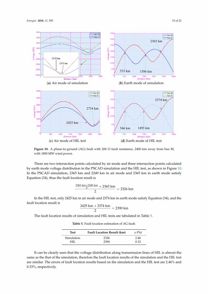
Figure 10. A phase-to-ground (AG) fault with 200 Ω fault resistance, 2400 km away from bus M, with 1800 MW wind power.

There are two intersection points calculated by air mode and three intersection points calculated by earth mode voltage distribution in the PSCAD simulation and the HIL test, as shown in Figure 10. In the PSCAD simulation, 2365 km and 2249 km in air mode and 2365 km in earth mode satisfy Equation (34), thus the fault location result is

2365 km 2249 km 2365 km2 2326 km

2

+ +=

In the HIL test, only 2425 km in air mode and 2374 km in earth mode satisfy Equation (34), and the fault location result is

2425 km 2374 km 2390 km2+ =

The fault location results of simulation and HIL tests are tabulated in Table 5.

Table 5. Fault location estimation of AG fault.

Test Fault Location Result (km) ε (%) Simulation 2326 2.46

HIL 2390 0.33

It can be clearly seen that the voltage distribution along transmission lines of HIL is almost the same as the that of the simulation, therefore the fault location results of the simulation and the HIL test are similar. The errors of fault location results based on the simulation and the HIL test are 2.46% and 0.33%, respectively.

0 500 1000 1500 2000 2500 30000

500

1000

1500

2000

2500

3000

3500

distance (km)

volta

ge (k

V)

bus Mbus N

533 km 1586 km

2365 km

0 500 1000 1500 2000 2500 30000

1000

2000

3000

4000

5000

6000

volta

ge (k

V)

distance (km)

bus Mbus N

2425 km

2734 km

0 500 1000 1500 2000 2500 30000

500

1000

1500

2000

2500

volta

ge (k

V)

distance (km)

bus Mbus N

546 km 1493 km

2374 km

Figure 10. A phase-to-ground (AG) fault with 200 Ω fault resistance, 2400 km away from bus M,with 1800 MW wind power.

There are two intersection points calculated by air mode and three intersection points calculatedby earth mode voltage distribution in the PSCAD simulation and the HIL test, as shown in Figure 10.In the PSCAD simulation, 2365 km and 2249 km in air mode and 2365 km in earth mode satisfyEquation (34), thus the fault location result is

2365 km+2249 km2 + 2365 km

2= 2326 km

In the HIL test, only 2425 km in air mode and 2374 km in earth mode satisfy Equation (34), and thefault location result is

2425 km + 2374 km2

= 2390 km

The fault location results of simulation and HIL tests are tabulated in Table 5.

Table 5. Fault location estimation of AG fault.

Test Fault Location Result (km) ε (%)

Simulation 2326 2.46HIL 2390 0.33

It can be clearly seen that the voltage distribution along transmission lines of HIL is almost thesame as the that of the simulation, therefore the fault location results of the simulation and the HIL testare similar. The errors of fault location results based on the simulation and the HIL test are 2.46% and0.33%, respectively.

Energies 2018, 11, 593 16 of 22

5.3. Phase-to-Phase Fault

A phase-A-to-phase-B (AB) fault with 10 Ω fault resistance, 300 km away from bus M, whichoccurred with 210 MW wind power at 20 s, was investigated. The calculated voltage distributionsalong transmission lines from bus M and bus N are given in Figure 11.

Energies 2018, 11, x FOR PEER REVIEW 16 of 21

5.3. Phase-to-Phase Fault

A phase-A-to-phase-B (AB) fault with 10 Ω fault resistance, 300 km away from bus M, which occurred with 210 MW wind power at 20 s, was investigated. The calculated voltage distributions along transmission lines from bus M and bus N are given in Figure 11.

(a) Air mode of simulation (b) Air mode of HIL test

Figure 11. A phase-A-to-phase-B (AB) fault with 10 Ω fault resistance, 300 km away from bus M, with 210 MW wind power.

The AB fault point is nearly ideal, thus the minimums of air modal and earth modal voltage distribution along transmission lines are similar. In the PSCAD simulation, 300 km and 298 km are the minimum in air mode, hence the fault location result is

298 3000 300298 km 300 km 300 km3000 3000

−× + × =

In the HIL test, 261 km and 300 km are the minimum in air mode, and the fault location result is

261 3000 300261 km 300 km 294 km3000 3000

−× + × =

Table 6 demonstrates the fault location results of the simulation and the HIL tests.

Table 6. AB fault location results of simulation and HIL test.

Test Fault Location Result (km) ε (%) Simulation 300 0.00

HIL 294 0.20

The AB fault point is a nearly ideal boundary for the air mode circuit containing phase A and phase B, thus the minimums of air modal and earth modal voltage distribution along transmission lines are similar. The fault location error of the simulation is 0.00 and of the HIL test is 0.20. Even though the error of the HIL test is larger than that of the simulation, it is acceptable.

5.4. Double Phase-to-Ground Fault

A double phase-to-ground (ABG) fault with 50 Ω fault resistance, 1500 km away from bus M was studied, while fault occurred at 30 s with 400 MW produced wind power. The calculated voltage distributions along transmission lines from bus M and bus N are presented in Figure 12.

0 500 1000 1500 2000 2500 3000-5000

0

5000

10000

15000

volta

ge(k

V)

distance(km)

bus Mbus N

298 km

300 km0 500 1000 1500 2000 2500 3000

0

1000

2000

3000

4000

5000

6000

7000

volta

ge (k

V)

distance (km)

bus Mbus N

300 km

261 km

Figure 11. A phase-A-to-phase-B (AB) fault with 10 Ω fault resistance, 300 km away from bus M, with210 MW wind power.

The AB fault point is nearly ideal, thus the minimums of air modal and earth modal voltagedistribution along transmission lines are similar. In the PSCAD simulation, 300 km and 298 km are theminimum in air mode, hence the fault location result is

298 km× 2983000

+ 300 km× 3000− 3003000

= 300 km

In the HIL test, 261 km and 300 km are the minimum in air mode, and the fault location result is

261 km× 2613000

+ 300 km× 3000− 3003000

= 294 km

Table 6 demonstrates the fault location results of the simulation and the HIL tests.

Table 6. AB fault location results of simulation and HIL test.

Test Fault Location Result (km) ε (%)

Simulation 300 0.00HIL 294 0.20

The AB fault point is a nearly ideal boundary for the air mode circuit containing phase A andphase B, thus the minimums of air modal and earth modal voltage distribution along transmission linesare similar. The fault location error of the simulation is 0.00 and of the HIL test is 0.20. Even thoughthe error of the HIL test is larger than that of the simulation, it is acceptable.

5.4. Double Phase-to-Ground Fault

A double phase-to-ground (ABG) fault with 50 Ω fault resistance, 1500 km away from bus Mwas studied, while fault occurred at 30 s with 400 MW produced wind power. The calculated voltagedistributions along transmission lines from bus M and bus N are presented in Figure 12.

Energies 2018, 11, 593 17 of 22Energies 2018, 11, x FOR PEER REVIEW 17 of 21

(a) Air mode of simulation (b) Earth mode of simulation

(c) Air mode of HIL test (d) Earth mode of HIL test

Figure 12. A double phase-to-ground (ABG) fault with 50 Ω fault resistance, 1500 km away from bus M, with 400 MW wind power.

Here, both the intersection points and minimum method can be applied for fault location estimation of ABG fault. In the PSCAD simulation, the intersection point in air mode, 1495 km, and minimums, 1556 km and 1573 km, are all close to 1502 km, one of the intersection points in earth mode voltage distribution, therefore the fault location result is

1556 3000 15731495 km+1556 km 1573 km3000 3000 1552 km

2

−× + ×=

In the HIL test, the intersection point in air mode is 1553 km and the minimums are 1499 km and 1560 km. The fault location result is

1560 3000 14991553 km+1560 km 1499 km3000 3000 1551 km

2

−× + ×=

The fault location results of the simulation and the HIL tests are illustrated in Table 7.

Table 7. Location results of ABG fault.

Test Fault Location Result (km) ε (%) Simulation 1552 1.76

HIL 1551 1.76

Here, both the intersection points and minimum method can be applied for fault location estimation. Lastly, the fault location results of the simulation and the HIL test are almost the same, and fault location errors are both 1.76%.

0 500 1000 1500 2000 2500 30000

100

200

300

400

500

600

700

800

900

volta

ge (k

V)

distance (km)

bus Mbus N619 km

1502 km 2454 km

0 500 1000 1500 2000 2500 30000

200

400

600

800

1000

1200

volta

ge (k

V)

distance (km)

bus Mbus N560 km

2388 km1475 km

Figure 12. A double phase-to-ground (ABG) fault with 50 Ω fault resistance, 1500 km away from busM, with 400 MW wind power.

Here, both the intersection points and minimum method can be applied for fault locationestimation of ABG fault. In the PSCAD simulation, the intersection point in air mode, 1495 km,and minimums, 1556 km and 1573 km, are all close to 1502 km, one of the intersection points in earthmode voltage distribution, therefore the fault location result is

1495 km + 1556 km× 15563000 + 1573 km× 3000−1573

30002

= 1552 km

In the HIL test, the intersection point in air mode is 1553 km and the minimums are 1499 km and1560 km. The fault location result is

1553 km + 1560 km× 15603000 + 1499 km× 3000−1499

30002

= 1551 km

The fault location results of the simulation and the HIL tests are illustrated in Table 7.

Table 7. Location results of ABG fault.

Test Fault Location Result (km) ε (%)

Simulation 1552 1.76HIL 1551 1.76

Here, both the intersection points and minimum method can be applied for fault locationestimation. Lastly, the fault location results of the simulation and the HIL test are almost the same,and fault location errors are both 1.76%.

Energies 2018, 11, 593 18 of 22

5.5. Three-Phase Fault

A three-phase (ABC) fault with 10 Ω fault resistance, 1800 km away from bus M, was simulatedat 50 s, with 550 MW produced wind power. The calculated voltage distribution along transmissionlines from bus M and bus N are illustrated in Figure 13, and the fault location estimations are providedin Table 8.

Energies 2018, 11, x FOR PEER REVIEW 18 of 21

5.5. Three-Phase Fault

A three-phase (ABC) fault with 10 Ω fault resistance, 1800 km away from bus M, was simulated at 50 s, with 550 MW produced wind power. The calculated voltage distribution along transmission lines from bus M and bus N are illustrated in Figure 13, and the fault location estimations are provided in Table 8.

(a) Air mode of simulation (b) Air mode of HIL test

Figure 13. A three-phase (ABC) fault with 10 Ω fault resistance, 1800 km away from bus M, with 550 MW wind power.

Only minimums of voltage distributions are applied in this case, but all the minimums are close to the fault point. In the PSCAD simulation, the minimums are 1788 km and 1809 km, so the fault location result is obtained as

1809 3000 17881809 km 1788 km 1799 km3000 3000

−× + × =

In the HIL test, the minimums are 1741 km and 1799 km, and the fault location result is

1741 3000 17991741 km 1799 km 1765 km3000 3000

−× + × =

The fault location results of the simulation and the HIL test can be found in Table 8.

Table 8. Location estimation of ABC fault.

Test Fault Location Result (km) ε (%) Simulation 1799 0.03

HIL 1765 1.17

The minimums of air voltage distributions are similar in the simulation and the HIL test, so the minimums are applied to estimate the fault location. The fault location error of the simulation is just 0.03%, which is smaller than that of the HIL test; however, the fault location error of the HIL test is just 1.17% and acceptable in the practical implementation.

Comprehensive simulations and HIL tests in the presence of different fault distances, resistances, types, and wind power penetration were carried out to fully verify the effectiveness of MVD-ADFL, which are only summarized in Table 9 due to page limits.

Figure 13. A three-phase (ABC) fault with 10 Ω fault resistance, 1800 km away from bus M,with 550 MW wind power.

Only minimums of voltage distributions are applied in this case, but all the minimums are closeto the fault point. In the PSCAD simulation, the minimums are 1788 km and 1809 km, so the faultlocation result is obtained as

1809 km× 18093000

+ 1788 km× 3000− 17883000

= 1799 km

In the HIL test, the minimums are 1741 km and 1799 km, and the fault location result is

1741 km× 17413000

+ 1799 km× 3000− 17993000

= 1765 km

The fault location results of the simulation and the HIL test can be found in Table 8.

Table 8. Location estimation of ABC fault.

Test Fault Location Result (km) ε (%)

Simulation 1799 0.03HIL 1765 1.17

The minimums of air voltage distributions are similar in the simulation and the HIL test, so theminimums are applied to estimate the fault location. The fault location error of the simulation is just0.03%, which is smaller than that of the HIL test; however, the fault location error of the HIL test is just1.17% and acceptable in the practical implementation.

Comprehensive simulations and HIL tests in the presence of different fault distances, resistances,types, and wind power penetration were carried out to fully verify the effectiveness of MVD-ADFL,which are only summarized in Table 9 due to page limits.

Energies 2018, 11, 593 19 of 22

Table 9. Fault location results of simulation and HIL test.

Fault Distance (km) 100 200 500 450 650 720 830 1020 1675 1740 2200 2900Produced Wind Power (MW) 120 500 180 300 550 280 600 400 140 570 450 350

Fault Type AG AB ABC ABG AG ABC ABG AB ABC AG AB AGFault Resistance (Ω) 200 0 100 50 20 30 10 20 10 80 20 100

Fault Location Result of Simulation (km) 114 201 531 463 618 721 877 1012 1699 1711 2184 2868ε of Simulation (%) 0.50 0.03 1.03 0.43 1.07 2.30 1.57 0.27 0.8 0.97 0.53 1.07

Fault Location Result of HIL Test (km) 111 213 527 469 615 725 868 1034 1681 1770 2177 2851ε of HIL Test (%) 0.37 0.43 0.90 0.63 1.17 0.17 1.27 0.47 0.13 1.00 0.77 1.67

Due to the ideal boundary formed by at least two conductors in the case of air mode of AB andABC, the MVD-ADFL fault location results of AB and ABC faults are better than those of AG andABG faults. Additionally, HIL tests and PSCAD simulation are based on different electromagnetictransient program engines, thus some fault location results of HIL tests are even better than those ofthe PSCAD simulation. Considering the inevitable high-frequency noise in the data acquisition ofHIL tests, the good performance of MVD-ADFL in HIL tests indicates that the proposed fault locationmethod is not sensitive enough to the high-frequency noise in the voltage and current waveforms.

6. Discussion

6.1. Adaptability of MVD-ADFL for Any Long Transmission Lines

AC transmission lines cannot be any longer due to the cost of compensation increasing rapidlywith line distance, thus traditional AC transmission lines between two substations are dozens tohundreds of kilometers, which is much shorter than the half-wavelength of power system frequency.As a result, there will generally be only one intersection point in either air mode or earth modevoltage distribution if the fault location method based on voltage distribution is applied in traditionaltransmission lines, as shown in [1]. Furthermore, the different intersection points of earth modeand air mode are utilized to identify the right fault location results in HWTL fault location, but thisidentification process is unnecessary due to there being only one intersection point in each mode.

6.2. Generator Type

The wind turbine was selected in this paper because the integration of large-scale wind poweris a prominent issue for further development of wind energy in China. Electricity transmission fromnorthern China to the load centers in the coastal region is quite inefficient, and the local electricityconsumption capability is extremely insufficient due to extreme weather and geographical conditions.Therefore, half-wavelength transmission lines are proposed for bulk wind power transmission, andthe wind generator was chosen as the background for our half-wavelength transmission line faultlocation study. Additionally, due to the wide implementation of doubly fed induction generators inlarge-scale wind farms, these are applied as the wind turbine type in this study.

The proposed MVD-ADFL method is based on the angle and magnitude of the fundamentalfrequency voltage and current, which vary with the power generated by wind turbines. The generatedpower depends on wind speed, which is unstable and unpredictable in most cases. The frequentvariation of electrical power, which is rare in solar, hydro, and fossil fuel power generation processes,can be seen as a disturbance to the stable frequency component and an unfavorable factor in thefundamental frequency–based fault location method, therefore wind turbines can reduce the accuracyof the proposed method.

7. Conclusions

In this paper, an MVD-ADFL was developed for HWTL with large-scale wind power integration.The main contributions of this paper can be summarized into the following four aspects:

Energies 2018, 11, 593 20 of 22

(1) The proposed MVD-ADFL is based on transmission line parameters and voltage and current atfundamental frequency. Therefore, traditional low-frequency voltage and current measurementdevices are applicable to MVD-ADFL, which offers wide implementation in practice.

(2) The application of voltage amplitude avoids the accurate synchronization of double-end voltageand current. If synchronous voltage and current are available, they can be used to further reducecalculation errors in fault location.

(3) Simulation results of different case studies have verified that MVD-ADFL is quite effective fordifferent fault types, while it is insensitive to fault distance, fault resistance, and stochastic windpower variation.

(4) The RTDS-based HIL test validates the feasibility of implementing MVD-ADFL in different cases.

Future study will investigate the asymmetrical characteristics of non-ideally transposed line toimprove the fault location performance of MVD-ADFL in a more practical scenario.

Acknowledgments: The authors gratefully acknowledge the support of the National Natural Science Foundationof China (51667010) and Yunnan Provincial Talents Training Program (KKSY201604015).

Author Contributions: Preparation of the manuscript has been performed by Pulin Cao, Hongchun Shu, Bo Yang,Na An, Dalin Qiu, Weiye Teng, and Jun Dong.

Conflicts of Interest: The authors declare no conflict of interest.

References

1. Yang, B.; Sang, Y.Y.; Shi, K.; Yao, W.; Jiang, L.; Yu, T. Design and real-time implementation of perturbationobserver based sliding-mode control for VSC-HVDC systems. Control Eng. Pract. 2016, 56, 13–26. [CrossRef]

2. Han, Y.; Xu, C.; Xu, G.; Zhang, Y.W.; Yang, Y.P. An improved flexible solar thermal energy integration processfor enhancing the coal-based energy efficiency and NOx removal effectiveness in coal-fired power plantsunder different load conditions. Energies 2017, 10, 1485. [CrossRef]

3. Hooman, K.; Huang, X.X.; Jiang, F.M. Solar-enhanced air-cooled heat exchangers for geothermal powerplants. Energies 2017, 10, 1676. [CrossRef]

4. Maheshwari, Z.; Ramakumar, R. Smart integrated renewable energy systems (SIRES): A novel approach forsustainable development. Energies 2017, 10, 1145. [CrossRef]

5. Ligus, M. Evaluation of economic, social and environmental effects of low-emission energy technologiesdevelopment in Poland: A multi-criteria analysis with application of a fuzzy analytic hierarchy process.Energies 2017, 10, 1550. [CrossRef]

6. Yao, W.; Jiang, L.; Wen, J.Y.; Wu, Q.H.; Cheng, S.J. Wide-area damping controller for power system inter-areaoscillations: A networked predictive control approach. IEEE Trans. Control Syst. Technol. 2015, 23, 27–36.[CrossRef]

7. Yang, B.; Yu, T.; Shu, H.C.; Zhang, Y.M.; Chen, J.; Sang, Y.Y.; Jiang, L. Passivity-based sliding-mode controldesign for optimal power extraction of a PMSG based variable speed wind turbine. Renew. Energy 2018, 119,577–589. [CrossRef]

8. Chinese Electric Almanac Committee. Chinese Electric Almanac in 2016; China Electric Power Press: Beijing,China, 2017; pp. 526–528. (In Chinese)

9. Yang, B.; Jiang, L.; Wang, L.; Yao, W.; Wu, Q.H. Nonlinear maximum power point tracking control and modalanalysis of DFIG based wind turbine. Int. J. Electr. Power Energy Syst. 2016, 74, 429–436. [CrossRef]

10. Yang, B.; Yu, T.; Su, H.; Jiang, L. Robust sliding-mode control of wind energy conversion systems for optimalpower extraction via nonlinear perturbation observers. Appl. Energy 2018, 210, 711–723. [CrossRef]

11. Santos, M.L.; Jardini, J.A.; Casolari, R.P.; Vasquez-Arnez, R.L.; Saiki, G.Y.; Sousa, T.; Nicola, G.L.C.Power transmission over long distances: Economic comparison between HVDC and half-wavelengthline. IEEE Trans. Power Deliv. 2017, 29, 502–509. [CrossRef]

12. Yang, B.; Zhang, X.S.; Yu, T.; Shu, H.C.; Fang, Z.H. Grouped grey wolf optimizer for maximum power pointtracking of doubly-fed induction generator based wind turbine. Energy Convers. Manag. 2017, 133, 427–443.[CrossRef]

Energies 2018, 11, 593 21 of 22

13. Fabián, R.G.; Tavares, M.C. Faulted phase selection for half-wavelength power transmission lines. IEEE Trans.Power Deliv. 2017. [CrossRef]

14. Silva, E.; Moreira, F.; Tavares, M. Energization simulations of a half-wavelength transmission line whensubject to three-phase faults—Application to a field test situation. Electr. Power Syst. Res. 2016, 138, 58–65.[CrossRef]

15. Mauricio, A.; Robson, D. FACTS for Tapping and Power Flow Control in Half-Wavelength TransmissionLines. IEEE Trans. Ind. Electron. 2012, 59, 3669–3679.

16. Prabhakara, F.S.; Parthasarathy, K.; Rao, H.N.R. Performance of tuned half-wave-length power transmissionlines. IEEE Trans. Power Appar. Syst. 2007, PAS-88, 1795–1802. [CrossRef]

17. Zhao, Y.X.; Wang, S.F.; Wang, H.X.; Wang, J.; Chen, A.Y.; Xue, T.S. Study on the resettlement modes ofhalf-wavelength tuned network of transmission lines. Electr. Power 2017, 50, 147–152. (In Chinese)

18. Jiao, C.; Qi, L.; Cui, X. Compensation technology for electrical length of half-wavelength AC powertransmission lines. Power Syst. Technol. 2011, 142, 467–470. (In Chinese)

19. Wang, Y.; Xu, W.; Li, Y.W.; Hao, T. High-frequency, half-wavelength power transmission scheme. IEEE Trans.Power Deliv. 2017, 32, 279–284. [CrossRef]

20. Zhang, Z.J.; You, J.W.; Zhao, J.Y.; Cheng, Y.; Jiang, X.L.; Li, Y.F. Contamination characteristics ofdisc-suspension insulator of transmission line in wind tunnel. IET Gener. Transm. Distrib. 2017, 11, 1453–1460.[CrossRef]

21. Liu, Z.; Liang, K.; Mezentsev, A.; Enno, S.; Sugier, J.; Füllekrug, M. Variable phase propagation velocity forlong-range lightning location system. Radio Sci. 2016, 51, 1806–1815. [CrossRef]

22. Li, P.; Huang, D.C.; Ruan, J.J.; Wei, H.; Qin, Z.H.; Long, M.Y.; Pu, Z.H.; Wu, T. Influence of forest fire particleson the breakdown characteristics of air gap. IEEE Trans. Dielectr. Electr. Insul. 2016, 23, 1974–1984. [CrossRef]

23. Rui, X.M.; Ji, K.P.; Li, L.; McClure, G. Dynamic response of overhead transmission lines with eccentric icedeposits following shock loads. IEEE Trans. Power Deliv. 2017, 32, 1287–1294. [CrossRef]

24. Izykowski, J.; Rosolowski, E.; Balcerek, P.; Fulczyk, M.; Saha, M.M. Accurate noniterative fault locationalgorithm utilizing two end unsynchronized measurements. IEEE Trans. Power Deliv. 2010, 26, 547–555.[CrossRef]

25. Wang, L.; Suonan, J. A fast algorithm to estimate phasor in power systems. IEEE Trans. Power Deliv. 2017, 32,1147–1156. [CrossRef]

26. Danilo, P.; Christo, E.S.; Almeida, R. Location of faults in power transmission lines using the ARIMA method.Energies 2017, 10, 1596.

27. Serrano, J.; Platero, C.; López-Toledo, M.; Granizo, R. A new method of ground fault location in 2 × 25 kVrailway power supply systems. Energies 2017, 10, 340. [CrossRef]

28. Bhatti, A.A. Fault location in active distribution networks using non-synchronized measurements. Int. J.Electr. Power Energy Syst. 2017, 93, 451–458.

29. Swaroop, G.; Ashok, P. An Accurate Fault Location Method for Multi-Circuit Series CompensatedTransmission Lines. IEEE Trans. Power Syst. 2017, 32, 572–580.

30. Zhao, P.; Chen, Q.; Sun, K.; Xi, C.A. Current frequency component-based fault-location method forvoltage-source converter-based high-voltage direct current (VSC-HVDC) cables using the s transform.Energies 2017, 10, 115. [CrossRef]

31. Saha, M. Fault Location on Power; Springer Press: London, UK, 2009; pp. 52–54.32. Yang, B.; Hu, Y.L.; Huang, H.Y.; Shu, H.C.; Yu, T.; Jiang, L. Perturbation estimation based robust state

feedback control for grid connected DFIG wind energy conversion system. Int. J. Hydrogen Energy 2017, 42,20994–21005. [CrossRef]

33. Shen, Y.; Yao, W.; Wen, J.Y.; He, H.B. Adaptive wide-area power oscillation damper design for photovoltaicplant considering delay compensation. IET Gener. Transm. Distrib. 2017. [CrossRef]

34. Liao, S.W.; Yao, W.; Han, X.N.; Wen, J.Y.; Cheng, S.J. Chronological operation simulation framework forregional power system under high penetration of renewable energy using meteorological data. Appl. Energy2017, 203, 816–828. [CrossRef]

35. Liu, J.; Wen, J.Y.; Yao, W.; Long, Y. Solution to short-term frequency response of wind farms by using energystorage systems. IET Renew. Power Gener. 2016, 10, 669–678. [CrossRef]

Energies 2018, 11, 593 22 of 22

36. Yang, B.; Yu, T.; Zhang, X.S.; Huang, L.N.; Shu, H.C.; Jiang, L. Interactive teaching-learning optimizer forparameter tuning of VSC-HVDC systems with offshore wind farm integration. IET Gener. Transm. Distrib.2018, 12, 678–687. [CrossRef]

37. Yang, B.; Yu, T.; Shu, H.C.; Zhang, X.S.; Qu, K.P.; Jiang, L. Democratic joint operations algorithm for optimalpower extraction of PMSG based wind energy conversion system. Energy Convers. Manag. 2018, 159, 312–326.[CrossRef]

38. Liu, Z. Overvoltage and Insulation of Ultra-High Voltage AC Transmission Lines; China Electric Power Press:Beijing, China, 2014; p. 49. (In Chinese)

© 2018 by the authors. Licensee MDPI, Basel, Switzerland. This article is an open accessarticle distributed under the terms and conditions of the Creative Commons Attribution(CC BY) license (http://creativecommons.org/licenses/by/4.0/).