Volatility Term Structures in Commodity Markets

Volatility Term Structures in Commodity Markets∗

Fabian Hollstein†, Marcel Prokopczuk†,‡ and Christoph Wursig†

ABSTRACT

In this study, we comprehensively examine the volatility term structures in commodity mar-

kets. We model state-dependent spillovers in principal components (PCs) of the volatility

term structures of different commodities, as well as that of the equity market. We detect

strong economic links and a substantial interconnectedness of the volatility term structures of

commodities. Accounting for intra-commodity-market spillovers significantly improves out-

of-sample forecasts of the components of the volatility term structure. Spillovers following

macroeconomic news announcements account for a large proportion of this forecast power.

There thus seems to be substantial information transmission between different commodity

markets.

JEL classification: G10, G14, G17.

Keywords: Commodities, information transmission, spillovers, volatility term structure

∗We thank Bob Webb (the editor) as well as an anonymous referee and participants atthe Commodity Markets Winter Workshop in Hannover for their constructive comments. Con-tact: [email protected] (F. Hollstein), [email protected] (M. Prokopczuk),[email protected] (C. Wursig).†School of Economics and Management, Gottfried Wilhelm Leibniz University of Hanover,

Koenigsworther Platz 1, 30167 Hannover, Germany.‡ICMA Centre, Henley Business School, University of Reading, Reading RG6 6BA, UK.

Electronic copy available at: https://ssrn.com/abstract=3491715

I. Introduction

A large set of external events and conditions has the potential to affect commodity mar-

kets. Important drivers of commodity prices are, inter alia, weather, investor flows and

macroeconomic conditions. While the level of commodity prices is certainly important, un-

derstanding the volatility of commodity prices is at least as crucial. For example, Pindyck

(2004) shows that, because storage helps to smooth production and deliveries, the marginal

value of storage increases with volatility. Further applications where volatility is of special

concern include risk management decisions, margin calculations, or the valuation of options

contracts. While previous studies have examined the impact of commodity spot volatil-

ity, the entire volatility term structure provides additional important information for the

above mentioned issues, since short-term and long-term options embed partly differential

information and provide market expectations of future volatility over various horizons.

The importance of considering the entire term structure has been widely documented

for equity markets (e.g. Adrian and Rosenberg, 2008; Bakshi, Panayotov, and Skoulakis,

2011; Feunou, Fontaine, Taamouti, and Tedongap, 2013). In particular, these studies show

that the volatility term structure is informative about, inter alia, risk premia, measures of

real economic activity, business cycle risk and the tightness of financial constraints. Inves-

tigating the interconnectedness of the term structure and its relation with macroeconomic

variables and announcements can be crucial to help understand the interdependencies and

macroeconomic links of the commodity markets. This can be particularly helpful for prac-

titioners that can use predictability of the entire volatility term structure for more accurate

risk evaluations of their portfolios.

Our main contribution is to provide a comprehensive study of the volatility term struc-

ture of different commodity markets. The volatility term structure is of special interest for

commodity markets because of its relation with the so called Samuelson (1965) effect. This

effect states that volatility generally decreases with increasing time to maturity. In appre-

ciating this, we can enhance our understanding of the determinants and dynamics of the

volatility term structure.

First, we decompose the volatility term structure into its principal components (PCs)

2


and study their economic drivers. We focus on the first three PCs: the level, the slope and

the curvature of the term structure. This analysis allows us to understand how volatility

dynamics change for contracts with different expiry dates.

When we investigate the macroeconomic determinants of the commodity volatility term

structure, we uncover two main results. (i) Macroeconomic variables can explain a large

proportion of the variation in the level factor, and typically a somewhat smaller share for

the slope and curvature factors. (ii) An increase in the proportion of speculative open interest

reduces the volatility level for various markets, while employment is positively related to the

volatility level.

Second, we use a state-dependent autoregressive (AR) model to examine volatility spillovers

between commodity markets. We compare a model using only the past lags of one commodity

volatility term structure to a state-dependent unrestricted AR-model which also includes the

lagged volatility PCs of another commodity, following the causality model by Granger (1969,

1988). We define economic states based on the forecast of the Engle and Manganelli (2004)

conditional autoregressive Value at Risk (CaViaR). Using the Granger (1969, 1988) causality

model to make out-of-sample predictions of the implied volatility term structure generally

yields sizable forecast improvements over the predictions of the simple state-dependent AR-

model. Accounting for spillover effects for the level and the slope yields out-of-sample R2s

of up to 5%. Intra-commodity effects are more important for the commodity market than

spillover effects originating from the equity market. Finally, spillovers are state-dependent:

they are strongest during market distress and smallest during normal periods.

One possible explanation for these findings is information transmission. To isolate the

effects originating from this channel, we investigate the impact of scheduled macroeconomic

news announcements on spillovers. If spillovers are larger after macroeconomic news an-

nouncements, this would indicate that some commodity markets capture information on

macroeconomic news earlier than others. This could lead to subsequent changes in the

volatility term structure of the cross-section of the commodity market. We find that macroe-

conomic news announcements models do indeed explain up to 70% of the spillovers for the

level. News announcements associated with consumer income or consumer sentiment have a

particularly large influence on spillovers for all components of the term structure.

3


We also investigate the impact of the financialization of commodity markets, which leads

to a stronger co-movement across commodities in recent years due to the increased use of

commodities as an investment (Tang and Xiong, 2012; Christoffersen, Lunde, and Olesen,

2019). We conduct a sub-sample analysis by studying changes in the lead/lag relationship

between commodity markets pre-and post-financialization, which reveals two main findings:

First, the volatility term structure for commodity and equity markets is strongly integrated

for the post-financialization period. Second, there are two effects that affect spillovers post-

financialization: (i) the increase in contemporaneous movements lowers spillovers for the

level and (ii) more common factors for the slope and the curvature lead to overall higher

spillovers.

Our study is related to several strands of the literature. For equity and bond markets

a variety of articles show that the variance term structure is important and can capture

unobserved risk factors. Adrian and Rosenberg (2008) and Bakshi et al. (2011) show that

factors that describe the volatility term structure can predict various economic and financial

measures. Bakshi et al. (2011) draw on an analogy with the term structure of interest rates

and argue that the variance term structure embodies expected variances by both the financial

and the real sector, as perceived by the index option market.1

For commodity markets, there is a vast literature that finds a factor structure in returns.

Rotemberg and Pindyck (1990), Yang (2013), Szymanowska, De Roon, Nijman, and Van

Den Goorbergh (2014) and Bakshi, Gao, and Rossi (2017) argue that common factors in

commodity markets can explain a large part of cross-sectional return variation. For their

analyses, these studies use the cross-section of commodity returns. Brunetti, Buyuksahin,

and Harris (2016) show that hedge funds positions are negatively related to the volatility in

corn, crude oil and natural gas futures markets. Hammoudeh and Yuan (2008) investigate

the effects of oil and interest rate shocks on the volatility of metals markets, using various

GARCH model specifications.

Our study extends this literature by investigating the entire volatility term structure

for a large cross-section of commodity markets. Leveraging the various expiration dates of

1Further studies on the volatility term structure in equity markets include: Campa and Chang (1995),Mixon (2007), Johnson (2017) and Hollstein, Prokopczuk, and Wese Simen (2019b).

4


commodity futures and options enables us to study the term structure and analyze whether

there is a common factor structure in the volatility term structure.

The central contribution of our paper is the analysis of the lead/lag factor structure of

commodity markets. Volatility spillovers of the commodity market have been investigated

in several studies, but only in relation to specific markets and to the volatility of the spot

market. Diebold and Yilmaz (2012) investigate volatility spillovers across different markets

using a generalized vector autoregressive (VAR) framework. Du and He (2015) investigate

Granger causality in risk between the returns of the crude oil market and stock market

returns. They find that after the financial crisis the crude oil market was positively linked to

the stock market, while it was negatively linked to the stock market beforehand. Nazlioglu,

Erdem, and Soytas (2013) investigate spillovers in spot volatility between oil and agricultural

markets. In the literature, spillovers are usually only investigated for certain events that

trigger an increased dependency between the markets – for example, the food crisis. One

reason for this might be that it is difficult to link spillovers to a particular cause. In this

study, we examine macroeconomic news announcements for exactly this purpose.

In doing so, we add to the literature that uses macroeconomic news announcements to

investigate the impact on returns or volatilities (Savor and Wilson, 2013; Lucca and Moench,

2015; Wachter and Zhu, 2018).

Finally, our study is related to the literature on financialization. Tang and Xiong (2012)

investigate the correlation between crude oil returns and other commodities, and find that

these correlations increase for a post-financialization period starting in 2004. Christoffersen

et al. (2019) investigate returns and variances of commodities in the post-financialization

period. They find that the factor structure is stronger for volatility, and that volatilities are

strongly related to stock market volatility and the business cycle. We extend this literature

by providing insights about the financialization of the entire commodity volatility term

structure and are able to capture a more complete picture than the previous literature. The

existing studies focus on contemporaneous movements, but not on the lead/lag relations in

the commodity market. We are the first study to investigate the impact of financialization

on the lead/lag structure of the commodity market volatility.

The remainder of this paper is organized as follows: In Section II we describe the data

5


and methodology. In Section III we present our main analysis and in Section IV we provide

robustness tests. Section V concludes.

II. Data and Methodology

A. Volatility Term Structures in Commodity Markets

We obtain the commodity futures and options dataset from the Commodity Research

Bureau (CRB). Our data covers the period from January 1st 1996 until December 31st 2015.

We consider the following commodities: cocoa, coffee, copper, corn, cotton, crude oil, gold,

natural gas, silver, soybeans and sugar. The selection of these commodities is based on the

need for a sufficient range of options over a reasonably long time period. Because we want to

study the impact of financialization on the lead/lag structure in the volatility term structure,

we require that commodities have option data before 2000. We exclude a commodity for a

certain year if the data coverage is below 70% of trading days.

We handle and filter the dataset following Prokopczuk, Symeonidis, and Wese Simen

(2017) and Hollstein, Prokopczuk, and Tharann (2019a) and remove all options that are in-

the-money, have a time to maturity of less than one week or have a price lower than five times

the minimum tick size. As risk-free rate, we use the daily Treasury yield.2 We further remove

observations that violate standard no-arbitrage conditions, as in Aıt-Sahalia and Duarte

(2003). Each day, we need to observe at least two out-of-the-money call- and put-options,

otherwise we remove this particular day from the sample. We follow Chang, Christoffersen,

Jacobs, and Vainberg (2011) and Hollstein and Prokopczuk (2016) to interpolate the implied

volatilities of options via cubic splines by moneyness (KF

), where K is the strike price and F

is the price of a future with the same maturity as the option. From this set of options we

calculate option prices using the Black (1976) formula. We use a constant extrapolation for

the moneyness levels above and below the daily maximum and minimum levels. As a result

we obtain a fine grid of 1000 implied volatilities between a moneyness of 1% and 300%. With

this dataset, we compute model–free implied volatilities. For the S&P 500, we use options

2https://www.treasury.gov/resource-center/data-chart-center/interest-rates/Pages/

TextView.aspx?data=yield.

6


https://www.treasury.gov/resource-center/data-chart-center/interest-rates/Pages/TextView.aspx?data=yield

https://www.treasury.gov/resource-center/data-chart-center/interest-rates/Pages/TextView.aspx?data=yield

data from OptionMetrics and apply the same procedure.

We compute model-free option-implied volatility for various maturities using the non-

parametric approach of Demeterfi, Derman, Kamal, and Zou (1999) and Britten-Jones and

Neuberger (2000) as:

V IX2t =

2Rft

T − t

[ ∫ Ft,T

0

1

K2pt,T (K)dK +

∫ ∞Ft,T

1

K2ct,T (K)dK

]. (1)

Rft is the continuously compounded risk-free rate and Ft,T is the futures price at date t for

maturity T . pt,T the put price and ct,T is the call price with strike K of respective out-of-

the-money options. For some commodities, volatility exhibits seasonality, which could have

a mechanical impact on the term structure as well as on spillover effects. To remove seasonal

effects, we use a trigonometric function, following Back, Prokopczuk, and Rudolf (2013):

kicos(ωgi(t, τ)− ωθi), (2)

where ω = 2π12

is the cycle length and gi(t, τ) = t + 12τ − Si[t+12τSi

]. The operator [X]

returns the largest integer which is not greater than x. ki is the specific exposure to the

season, θi is the peak of the seasonal structure and τ is the contract maturity. We set

Si to 12 corresponding to monthly seasonality. gi(t, τ) results therefore in integers from 0

to 11 representing the corresponding months. For each commodity, we regress the implied

volatility on the mechanical model implied by Equation (2) and retain the residual series.

Table I shows the summary statistics of the volatility term structures. One can observe

that the average volatility is decreasing with increasing maturity. This effect is strongest for

non-metal commodities. For metals, the term structure is relatively flat. For the equity mar-

ket, the volatility slightly increases with maturity. Thus the implied volatility term structure

for commodity markets has unique features which makes it interesting to investigate. The

standard deviation of the volatilities is lower for the annual maturities, except for gold, where

the standard deviation is constant. The first autoregressive component is usually larger for

longer-term volatilities, indicating a stronger persistence. This is not the case for energies,

where long-term volatilities are less persistent.

7


B. Macroeconomic Data

We use a similar approach as Stock and Watson (2012) to investigate the macroeconomic

determinants of the commodity volatility term structure. Specifically, we order various

macroeconomic variables into groups and obtain the first PC of each macroeconomic group.

In Table A1 of the Online Appendix, we describe the sources of our dataset as well as the

applied standardization technique. We obtain factors representing the following macroeco-

nomic groups: GDP components, Industrial production, Employment, Consumer expecta-

tions, Housing, Unemployment rate, Business inventories, Prices, Money supply, Interest

rates, Wages, Exchange rates, Stock prices and Financial conditions.

Additionally, we also consider the variance risk premium (VRP) of the equity market

(Bollerslev, Tauchen, and Zhou, 2009; Hollstein and Wese Simen, 2019). We use the monthly

VRP provided by Zhou (2018).3 The author defines the VRP as de-annualized V IX2 minus

the realized variance from 5-minute returns over the past month. For our set of macroeco-

nomic news announcements we use the most relevant macroeconomic news identified by the

Thompson Reuters Eikon Economic Monitor. We retain the announcement dates from the

webpages of the relevant institutions. We provide further details in Table A1 of the Online

Appendix.

C. Commodity-Specific Measures

Following Gorton, Hayashi, and Rouwenhorst (2012), we use the inventory data for the

commodity markets and several commodity-specific variables which are presented in Table

A1 of the Online Appendix. First, we use the volatility of the commodity market as a

whole. As a proxy we use the standard deviation of the CRB Commodity Index. Second,

we use a unique inventory variable for each commodity market, that is retained from the

sources presented in Table A1 of the Online Appendix. Third, motivated by Hong (2000)

we use the Commodity Futures Trading Commission (CFTC) dataset to calculate Working’s

(1960) T, as a measure of speculation. We use data on trader positions from the CFTC to

calculate the speculation factors. We use the historical dataset provided by the CFTC with

3https://sites.google.com/site/haozhouspersonalhomepage.

8


https://sites.google.com/site/haozhouspersonalhomepage

data from 1995 until 2015 that only distinguishes between commercial and non-commercial

traders. Table A1 of the Online Appendix shows the CFTC contract codes and associated

commodities. Following Gorton et al. (2012), we choose the newer contract when both

series are overlapping and we use the last value for the monthly observation. Speculation

is represented by the number of open interest from speculators, both long and short, NL

and NS divided by the open interest of hedgers (CL, CS). Working’s (1960) T is defined as

follows:

Working’s T =

1 +

NS

CS + CLif CS ≥ CL

1 +NL

CS + CLif CS < CL .

(3)

If the market is short (long), only short (long) speculators determine Working’s T.

Fourth, we use the basis of each commodity. Bakshi et al. (2017) show that this factor

helps to price the cross-section of commodities. To calculate the basis for every commodity,

we use the approach following Gorton et al. (2012) and Yang (2013) and define basis as the

log difference between the one-month futures price and the twelve-month futures price scaled

by the difference in time to maturity:

Bi,t =log(Fi,t,T1)− log(Fi,t,T2)

T2 − T1. (4)

The commodity basis reflects risk related to the convenience yield.

This results in the following factors: speculation, basis, commodity inventory and com-

modity volatility. For the purpose of calculating the basis, the dataset of futures is obtained

from the CRB and presented in Table A1 of the Online Appendix.

III. Main Analysis

A. Descriptive Analysis

Motivated by Cochrane and Piazzesi (2005), Feunou et al. (2013) and Johnson (2017),

we use information on the entire term structure to obtain unique factors of the implied

commodity volatility term structure. Option markets carry forward-looking information

9


about the underlying asset. Long-term and short-term options carry different information.

Schwartz and Smith (2000) argue that long-term futures contracts carry information about

the long-term equilibrium price level and short-term futures contracts provide information

about the short-term price variations. Long- and short-term option-implied volatility can be

interpreted in a similar vein.

We decompose the implied volatility term structure into three factors. The level factor

can be seen as average volatility and is influenced less by short-term fluctuations than the

slope, which loads positively on short-term volatility. In addition, we examine a curvature

factor. Dissecting the different effects of the volatility term structure will help to reduce

noise and provide insight into the information transmission and causal links of volatility for

the commodity market.

We calculate the factors with principal component analysis (PCA), which disentangles

term structure effects and creates uncorrelated orthogonal factors. All PCs are calculated

by singular value decomposition of the scaled data matrix. They are standardized to have

a mean of zero. Table II presents summary statistics that show that, combined, the three

PCs explain from 82% to 95% of the total variation of the term structure of option-implied

volatilities for the different commodities. In the following we separately examine the PCs.

Panel A of Table II shows that the level factor (first PC) captures 48% to 72% of the

variation in the term structure of option-implied volatilities. It captures most of the variation

for metals, where the Samuelson effect is not present (Bessembinder, Coughenour, Seguin,

and Smoller, 1996; Duong and Kalev, 2008). This factor is highly persistent, as evidenced by

the large AR(1) component. We use a factor rotation to ensure that the loadings on the first

PC are positive. Figure A1 of the Online Appendix shows the loadings of the level factor

on the components of the volatility term structure in black circles. The level factor has a

loading that is almost constant over time for all observed markets.

In Panel B of Table II we see that the slope factor (second PC) captures 15% to 21% of the

variation in the term structure of option-implied volatilities. The first-order autocorrelation

is lower compared to the level. However, while for the equity market the AR(1) coefficient

is only 0.79, for the commodity markets, the slope shows a higher autocorrelation of above

0.90. The loadings of the slope on the different contracts is displayed in blue triangles in

10


Figure A1 of the Online Appendix.4 These are consistently decreasing for all commodities,

except for natural gas. The slope should be positive when the Samuelson effect is present

and negative if it is not.

Panel C of Table II reveals that the curvature factor (third PC) can explain between

4% and 15% of the variation in the option-implied commodity volatility term structure. It

explains the highest share of the variation for softs and agricultural commodities, where the

Samuelson effect is strongest (Duong and Kalev, 2008). Surprisingly, the curvature factor

seems for most commodities not to be less persistent than the slope factor. Especially for

softs and agricultural commodities it has a higher persistence than for other sectors. The

first-order autocorrelation is larger than 0.9. In contrast, for the equity market the curvature

shows little first-order autocorrelation, with only 0.37. The loadings of the curvature factor

are displayed with an orange plus in Figure A1 of the Online Appendix.5 One can observe

that it displays a tent-shaped factor loading on the volatility term structure. The factor

loading is almost always highest for the nine-month implied volatility, with copper and gold

peaking at three and sugar peaking at six months.

To get an initial understanding of the dependence structure of the volatility term structure

across commodities, Table III presents the correlations of the level, slope and curvature

factors of different commodities. Additionally we investigate the correlation with the level

factor of each asset and the first PC of the entire cross-section. There is a strong factor

structure for the level of the volatility term structures. However, while there seems to be

a strong overall common factor structure, there are also cases of negative correlations in

the level factor across commodities. There is negative bi-variate correlation between coffee

and commodities in the metal market (copper, silver and gold). These results are consistent

with Christoffersen et al. (2019), who show that the common PC of the commodity market

realized volatility cannot explain a large degree of the realized volatility of coffee. The

correlations of the PCs of the volatility term structure of one commodity with those of other

commodities in the same sector are high for the metal market and the agricultural market.

4To have a consistent interpretation of the slope estimate for all markets, we require the slope of theterm structure to be downward sloping with maturity, otherwise we multiply the current rotation by −1.

5We require the curvature to have a larger loading for medium volatility compared to long- and short-termvolatility.

11


The sector components in the market for softs and energies are not as strong. We see a

strong factor structure in the slope of the volatility term structure with the first PC of the

slope: this correlation exceeds 0.2 for most commodities. The level and slope factors of the

equity market are also positively correlated with those of most commodity markets.

There are several questions that we seek to answer in the remainder of this paper: Are the

term-structure factors related to macroeconomic factors, sector-specific factors, or commod-

ity market factors? What are the determinants of the commodity volatility term structure?

Can the knowledge about today’s volatility term structure of one commodity help improve

forecasts for that of other commodities? What effect does financialization have on the com-

mon factor structure and the lead/lag factor structure? And, finally, Does information

transmission contribute to spillovers?

B. Macroeconomic Determinants

To shed light on the relationship of commodity volatility and the macroeconomy, we

conduct contemporaneous multivariate regressions of the level, slope and curvature factors

of each commodity on the macroeconomic variables discussed above. Several previous stud-

ies show that there is a relation between commodity volatility and macroeconmic variables.

Nguyen and Walther (2019) investigate the macroeconomic drivers of long- and short-term

volatility components. They find significant drivers for global real economic activity and

changes in consumer sentiment. Prokopczuk, Stancu, and Symeonidis (2019) and Kang,

Nikitopoulos, and Prokopczuk (2019) analyze economic drivers of commodity market volatil-

ity and crude oil volatility and find that volatility shows strong comovement with economic

and financial uncertainty, especially during crisis periods. For the softs and the agricultural

market Covindassamy, Robe, and Wallen (2017) and Adjemian, Bruno, Robe, and Wallen

(2018) show that macroeconomic variables and commodity-specific variables matter for the

volatility.

With certain variables – for example unemployment and employment – there could be

concerns about multicollinearity. To address this, we conduct the multicollinearity test of

Kovacs, Petres, and Toth (2005) and compute variance inflation factors (VIF). The Kovacs

et al. (2005) red indicator is a measure of redundancy, using the average correlation of the

12


data. For our sample, the average of this measure is 0.22, which is far below the threshold of

0.5 usually applied to diagnose multicollinearity. None of the VIFs exceeds 3.1 on average,

which is far below typical thresholds of 5 and 10 employed by the literature. Thus, these

tests indicate that the that multicollinearity does not pose a problem in the regressions.6

The results are shown Tables IV, V and VI, and we can see that certain macroeconomic

factors do indeed influence the volatility term structure.

Volatility Level: In Table IV we see that the level factor is in many cases negatively related

to the change in speculation, represented by Working’s T, albeit this change is insignificant.

There are several macroeconomic factors that influence the volatility term structure.

Employment is significantly positively related to the level factors of most commodities. For

sugar and corn, though, this effect is insignificant and for silver even negative. For the softs

market this also holds for unemployment, showing that the overall employment situation

seems to have a V-shaped influence on the level of volatilities for this market. High employ-

ment (unemployment) implies a high (low) available income and high (low) demand, which

results in increasing (increasing) expected variation in prices. These commodities are most

affected by direct consumer demand. Financial conditions are positively related to volatil-

ities of the metals market and sugar. They are negatively related to coffee, which might

explain the low correlation. This result is similar to those of Kilian (2009). The housing

market has a negative relationship with coffee, sugar and natural gas for the volatility level,

while the relation with the agricultural market and silver is positive. For interest rates, we

see a largely negative effect on the level of volatility. It is particularly large for metals that

are used for industrial purposes, e.g. copper and silver. Larger interest rates indicate larger

borrowing costs with, ceteris paribus, lower expected demand and lower variation. For gold,

an increase in interest rates increases opportunity costs and thus might result in decreasing

market demand. However, because gold is used primarily as a financial commodity, it does

not benefit from the positive signal of higher interest rates with regard to the stability of the

economy. This effect can, on the contrary, indicate that prices of gold fall further, because

the demand for hedges against an economic crisis decreases. This will likely result in in-

creasing volatilities. For other commodities this will not occur in the same magnitude when

6The detailed test results are available upon request.

13


inventories are not so low. For the volatility level of corn and gold, we see a negative relation

with money supply. The macroeconomic and commodity-specific factors are generally able

to explain a large part of the variation in the level factor. The R2s range between 34.52%

for gold and up to 57.75% for corn.

Volatility Slope: Table V shows the results for the slope of the implied commodity volatil-

ity term structures. According to the theory of storage, we would expect to have either a

significant positive relationship with the basis or a negative relationship with the inventory

variables. There are three hypothesis that explain when the Samuelson (1965) theory holds.

Hong (2000) states that information asymmetry in markets can lead to violations of the

Samuelson hypothesis. Fama and French (1988) argue that around business cycle peaks,

when inventory is low, the Samuelson hypothesis should hold, while the theory can be vio-

lated if inventory is high and marginal convenience yields are low. Bessembinder et al. (1996)

argue that the existence of a temporary component that is reversed over time is the main

factor that determines if the Samuelson hypothesis holds in a market. A positive shock leads

to a reversal over time. They find that the Samuelson hypothesis is empirically supported

in markets where spot price changes and the slope of the term structure co-vary negatively.

Tightening inventories reduces the possibility for markets to react to increases in demand or

supply shortages. Therefore we should investigate the basis, the inventory and Working’s T

with regard to their expected relation with the slope of the volatility term structure.

The basis is seen as a proxy for inventory levels. It is positive if the price of a one-month

contract is larger than the price of a twelve-month contract. This occurs when the commodity

is in backwardation, a state which is associated with tighter inventories. Contango, on the

other hand, is associated with abundant inventories. The theory of storage can be supported

for cocoa, silver, copper and natural gas. For these commodities we have either a significant

positive relationship with the basis or a negative relationship with the inventory variable.

The observations for gold, crude oil, corn and soybeans are not consistent with the theory

of storage.

For the slope, we see a negative relation of financial conditions for copper and silver. As

we have seen before, in good financial conditions the level of the volatility term structure

increases, while the term structure becomes increasingly flat. The market expects long-term

14


inventory to decrease, which leads to an increasing volatility in the future. We also observe a

significant negative relationship between many of the commodities and the housing market.

A housing crisis leads to a larger slope for sugar, cocoa, industrial metals and crude oil.

For the money supply, the largest relation can be seen in the slope. For coffee and sugar

there is a positive relationship. Corn, cotton, gold, silver and crude oil have a negative rela-

tionship. The higher the money supply the lower is the slope, so a higher money supply could

increase inflation expectations and long-term volatilities. For corn and gold an increasing

money supply leads to a lower overall level of the volatility term structure: the lower slope

indicates that the money supply particularly affects short-term volatilities for corn and gold.

For the slope, most variables have high explanatory value. However, part of the markets

for which the Samuelson hypothesis typically holds appear to be driven driven by idiosyn-

cratic factors (e.g. cocoa, coffee, cotton, corn and soybeans). For speculation we can observe

no effect for the entire market, in contrast to Hong (2000), who finds that information asym-

metry could lead to a violation of the Samuelson effect. He captures this effect in a model,

where hedgers trade without fundamental market information and speculators trade on their

information advantage. Uninformed hedgers trade for hedging reasons, which is why they

are willing to trade with informed investors. Due to a larger impact of non-marketed risk in

shorter-term futures. Hong (2000) further argues that cost in trading increases for the unin-

formed investor and they will trade less. He terms this effect a “speculative effect” that can

overwhelm the Samuelson effect, and this holds even assuming a homogeneous information

flow.

Volatility Curvature: The results for the curvature factor are shown in Table VI. The

curvature shows a positive relation with speculation only for corn. An increase in speculation

decreases the level of the term structure, and introduces a concave shape. For coffee, sugar

and corn the curvature is related to the exchange rate, for coffee and sugar a depreciating US-

Dollar is related to a concave term structure, and for corn this is related to a convex term

structure. Assuming that the Samuelson effect holds, this implies a higher medium-term

volatility for a negative relation and a lower medium-term volatility for a positive relation.

For coffee and sugar, the United States is a net importer, a depreciating currency will only

increase local demand and increase the price in US-Dollar. For corn the United States is

15


also a major exporter, having an effect on the cost of supply. For supplies, a depreciating

US-Dollar implies lower relative costs for producers in the United States, enabling them to

better compete and possibly increase supply. This has calming effects on the price volatility

for these commodities. The variables can generally explain a large share of the variation

in the curvature for the softs market. For the remaining commodity markets, the R2s are

generally smaller.

In summary, we find that macroeconomic variables can explain a large proportion of the

variation in the level factor, but typically somewhat smaller shares of the slope and curvature

factors.

C. Spillovers

Having documented a strong linear contemporaneous relationship between the volatility

term structure factors and macroeconomic determinants, we investigate whether there are

spillovers, i.e. lead/lag effects, in the volatility term structures. Volatility spillovers might

vary in different economic states. During periods of distress, macroeconomic effects likely

lead to a strong positive lead/lag relationship for most commodities. But the role of some

commodities during a crisis could be different. For example, gold is often seen as a hedge

against the equity market and might react differently to a macroeconomic shock than other

commodities.

We therefore investigate state-dependent spillovers in risk, using a Value at Risk (VaR)

approach. To construct state-dependent indicator variables we use the returns of an equally

weighted commodity portfolio with a 5% VaR. We use the resulting time series with the

percentiles of distressed or tranquil periods as in Adams, Fuss, and Gropp (2014). We

therefore consider three indicator variables, ID, IT and IN , for distress, tranquil and normal

periods, respectively. The variables are 1 if the VaR is in the defined α percentile. We follow

Adams et al. (2014) and define the lower bound as 12.5% and the upper bound as 75%. Thus

every observation below the 12.5% percentile indicates distress. Every observation above the

75% percentile indicates tranquil periods and everything in between shows normal economic

states.7 Adams et al. (2014) argue that these percentiles represent a good trade-off between

7This implies a transformation of the otherwise positively defined VaR, which we define to be negative.

16


power and an accurate representation of the state of the relevant market.

To estimate the VaR we use the CAViaR introduced by Engle and Manganelli (2004),

which is able to capture volatility clustering and time varying error distributions. Engle and

Manganelli (2004) specify the approach as follows:

V aRt(θ) = θ0 +

q∑j=1

θjV aRt−j(θ) +r∑i=1

θ(q+i)L(Yt−i). (5)

The AR components V aRt−j(θ) introduce persistence in the VaR series which assures its

continuity. The lag operator L(Yt−i) introduces the link to the underlying dataset. For our

purpose we use the asymmetric slope model by Engle and Manganelli (2004) as a specification

for L(Yt−i). This model is also used by Hong, Liu, and Wang (2009) for the estimation of the

VaR and is correctly specified for a GARCH process with asymmetrically modeled standard

deviation and i.i.d. errors. This is the specification of the asymmetric slope model:

V aRt(θl) = θ0 + θ1V aRt−1 + θ2Y+t−1 + θ3Y

−t−1 , (6)

where Y +t = max(Yt, 0), Y −t = −min(Yt, 0). The resulting 5% VaR estimate for an equally

weighted commodity portfolio is shown in Figure A2 of the Online Appendix. To obtain

coefficients for a spillover analysis, we estimate a regression following the spirit of Adams

et al. (2014). Our conditioning variable is not the LHS variable, but a commodity VaR

Index. Hence, we cannot use quantile regressions. Instead, as described above, we introduce

different economic states using dummy variables.

As control variables, we use the variance risk premium and the corresponding PC of the

17


equity market (PCE):8

PCi,t =

p∑k=1

β1kPCi,t−k · IN +

p∑k=1

β2kPCi,t−k · IT +

p∑k=1

β3kPCi,t−k · ID+

p∑u=1

γ1uPCj,t−u · IN +

p∑u=1

γ2uPCj,t−u · IT +

p∑u=1

γ3uPCj,t−u · ID+

V RPt + PCEt + εt.

(7)

PCi,t−k is the PC of asset i with lag k. We conclude that the term structure components

of assets j spill over to those of asset i if the following null hypotheses can be rejected. We

conduct four separate tests, with H0 : γ1u = 0 we test if we observe any significant spillover

effects during normal periods. For γ2u and γ3u we conduct the same test for tranquil and

distressed periods, respectively. Additionally, we conduct a test investigating whether all

three variables are jointly zero, H0 : γ1u = γ2u = γ3u = 0.

We further test whether the results are economically significant by performing an out-

of-sample test. We examine whether we can improve the forecast of the implied volatility

term structure when we have knowledge of the implied volatility term structure of another

commodity. We follow Goyal and Welch (2007) to conduct an out-of-sample analysis. We

test the forecast from the unrestricted AR regression including the components of asset j

against a restricted AR process that sets coefficients H0 : γ1u = γ2u = γ3u = 0. For the

purpose of the out-of-sample analysis, we assign the dummies based on forecasts that use

only information available at time t− 1.

We measure the out-of-sample performance with the following formula:

R2OOS = 1− MSEun

MSEre, (8)

where MSEun is the mean squared error of the unrestricted forecast and MSEre is the mean

squared error of the restricted forecast. The restricted model assumes that γ1u = γ2u = γ3u = 0

cannot be rejected.

8To uncover the relationship with the stock market we conduct a regression with the stock market’s PC.In this case, we treat it like a PC of a commodity and consequently drop the PC of the equity market (PCE)from the set of control variables.

18


We present the results of the state-dependent spillover test in Table VII. The level factor

is in Panel A, the slope factor in Panel B and the curvature factor in Panel C. If the

numbers are bold, the null hypothesis of zero predictability is rejected out-of-sample, using

the McCracken (2007) OOS-F statistics, with a significance level of 10%. The in-sample

significance is displayed with Newey and West (1986) standard errors with 10 lags. As

argued by Goyal and Welch (2007), in-sample predictability is a key requirement. Table VII

shows large bi-variate spillovers between commodity markets for the different term structure

factors. They are significant for a large number of commodities and large in size. Tables

A3, A4 and A5 of the Online Appendix further present the results of the out-of-sample tests

for the different economic states. Table VIII summarizes the information in these tables. In

general Table VIII shows that spillovers in distress are large in size, while during tranquil

periods they are large in frequency. Thus a state-dependent approach unveils differences in

spillovers between states.

Volatility Level: In the following, we discuss the spillovers in level (Panel A of Table

VII) in more detail. The equity market shows spillovers especially to commodity markets

that are related to the business cycle, like crude oil, silver, copper and gold. A prediction

that accounts for spillovers from the equity market to the gold, copper, crude oil and silver

markets yields out-of-sample R2s of 1.71%, 2.22%, 2.63% and 2.80%, respectively. A poten-

tial explanation for this finding is that the equity market reacts in a more timely manner to

changes in the business cycle. Robe and Wallen (2016) observe a similar linkage between the

equity markets and crude oil. We observe lagged information transmission to the business

cycle sensitive commodity markets. The spillovers are largest from the equity market in

periods of distress and normal periods, which can be seen in Table A3. In tranquil peri-

ods there is a feedback effect with the commodity market, indicating that the commodity

markets’ volatilities mainly influence the equity market in periods of low storage and tight

supply, that will likely occur in tranquil periods due to higher demand. For the level factor,

spillovers from the equity market decrease during tranquil periods while those to the equity

market are somewhat higher than in normal and distressed periods.

The term structure components of copper Granger cause those of commodities in the

same sector, crude oil and the equity market, which are connections we would expect from

19


a business cycle sensitive commodity like copper. Jacobsen, Marshall, and Visaltanachoti

(2019) show that metal returns lead equity markets. This connection to the equity market

can also be observed for the level of the volatility term structure. We also see substantial

spillovers from the gold market. In distress there are significant spillovers from gold to copper

and corn. In tranquil periods there are spillovers to cocoa and crude oil and during normal

periods to copper. Gold only spills over to silver in all economic states. The spillover to

cocoa might be linked to the influence of interest rates that the level of gold captures, as

can be seen in Table IV. This transmits to changes in the expected convenience yield, which

alters the expected level of inventory and results in changes for the level volatility of cocoa.

Corn and soybeans do not show a lot of sector commonalities for spillovers in level, but

both spill over to natural gas and gold. The link to natural gas might have something to

do with their role as a fertilizer and as a main energy source for drying crops after the

harvest. The larger the volatility, the higher is the incentive to produce more crops to

smooth production and deliveries, which results in the use of natural gas to dry crops faster.

Cotton captures demand-driven volatility fairly fast and thus spills over to the gold market,

especially during tranquil and distressed periods.

Cotton volatility Granger causes a lot of commodity markets and is, in turn, only Granger

caused by the volatility of three markets: crude oil, soybeans and sugar. Cotton Granger

causes especially natural gas, a link which is not obvious. However, there are several possi-

bilities. First, cotton is a competitor in the clothing industry with synthetic fibers that are

produced from natural gas. Second, both commodities are highly sensitive to the weather in

the United States, or more particularly in the Midwest, where a majority of the production

is located. Third, storms will increase the level for both commodities, introducing supply

disruptions to the market. Fourth, heatwaves decrease the harvest estimated for cotton and

increase energy demand due to cooling.

Sugar is linked to the softs market. The connection is especially large during distress.

One reason for this link might be the strong relationship of sugar to the housing market in

level that it shares with the rest of the softs market, for which the link is weaker. The level

of sugar causes also causes the level of crude oil. Both are linked due to biofuel production,

where sugar cane is an efficient alternative and Brazil can as a main producer of both ethanol

20


and sugar canes circumvent export restrictions for sugar by exporting ethanol.

The spillovers from crude oil to natural gas are small. This is in line with Bachmeier

and Griffin (2006), who find that there exists no common primary energy market. In level

the crude oil market spills over to every market. One reason for the high spillover is the

influence of institutional investors that invest more heavily in liquid business cycle related

markets. An indication for this can also be that crude oil is linked to the metal market

in all economic states. Evidence of that phenomenon can be seen in the literature on the

financialization of the commodity market. Basak and Pavlova (2016) show in a model that

shocks to index commodities spill over to prices and inventories of other index commodities.

Due to the influence on prices and inventories on volatility, this will also result in volatility

spillovers. Institutional investors can increase those spillovers via an increased correlation.

Volatility Slope: Panel B of Table VII displays the results for the slope. The equity

market is less connected to the commodity market, spilling over only to the agricultural

market and to precious metals. The slope of the equity volatility term structure cannot

capture the unique patterns of the commodity market. A majority of the spillovers occur

in tranquil periods, when the economic expansion that is reflected first in the stock market

leads to higher volatility in prices for the equity market and subsequently the commodity

market, as can be seen in Table VIII. Short-term volatility increases more strongly, when

inventory is tight (Fama and French, 1988). This effect spills over to the equity market from

the crude oil market and increases the slope as well, increasing the short-term uncertainty

of equity markets.

For the slope, spillovers from the equity market are higher than from the commodity

market. Copper, gold and silver all show spillovers that are lower for the slope compared to

the spillovers in level. This might be due to the low informativeness of the term structure for

metals compared to the level. The highest amount of spillovers can be seen during tranquil

periods, when inventory is low.

Spillovers to the slope of corn are large from coffee and cocoa, which shows short-term

macroeconomic information transmission. Coffee spills over to other markets especially dur-

ing periods of distress, which is an indication that coffee captures macroeconomic information

of the slope of the volatility term structure earlier, which influences other commodity mar-

21


kets in such periods. Gold and copper are likely Granger caused by cotton, because it can

capture a variety of general macroeconomic variables that can serve as early indicators for

the general economic activity as, for example, wages in the United States. Cotton is a labor-

intensive product with a high production share in the United States. Increases or decreases

in the wage will quickly be reflected in the volatility of the price and subsequently in the

demand for metals, which will affect volatility as well.

For the slope of the term structure, we still see a high degree of spillovers from crude oil

to other markets. The spillover to corn for the slope is large during normal periods and in

distress. This indicates that the short-term volatility of natural gas has a high influence on

the slope of corn, likely because of its use as a fertilizer. Large changes in the price of natural

gas can lead to large short-term changes in the price of corn; we have seen before that the

same holds for the level, where the effects on the average volatility seem to be stronger for

short-term volatilities.

Volatility Curvature: The main results for the curvature are in Panel C of Table VII. As

can be seen from Table VIII, there are significant spillover effects from the equity market

to all commodity markets in tranquil market periods. A shock to the term structure of the

equity market always spills over to the term structure of the commodity market, but we can

not observe spillover effects from the commodity market to the equity market. For the slope

and the curvature of the agricultural market, we observe more spillovers for corn than for

soybeans. The reason for this might be that corn captures relatively more macroeconomic

variables for the shape of the volatility term structure, while the shape of the term structure

of soybeans is idiosyncratic, as can be seen in Tables V and VI. Large links to natural gas

from the agricultural and softs markets show the medium-term impact of the volatility of

agricultural goods on the volatility of natural gas.

Summarizing the results, we see that spillovers are strongly dependent upon economic

states. They are strongest during market distress and comparably smallest in normal periods.

Furthermore, intra-commodity effects are more important for the commodity market than

spillover effects originating from the equity market. Intra-commodity effects rarely spill over

to the equity market.

22


D. Financialization

We now investigate the option-implied volatility term structure with regard to the fi-

nancialization of the commodity market. To do so, we split our sample into two parts.

January 2004 is often regarded as the break point of financialization (Hamilton and Wu,

2015; Christoffersen et al., 2019).9 In Table IX we display the correlations pre- and post-

financialization. At the bottom of each table we report the correlation of each variable with

the first PC of the entire market. We see that the difference between the two periods is stark.

In the grey colored post-financialization period the negative correlations disappear entirely

compared to the pre-financialization period. Correlations are mostly above 0.4. The corre-

lations of the factors of the term structure of natural gas and coffee with other commodities

are much lower – they are outliers in this regard. After financialization, the component is

large across commodities and (with the exception of coffee) above 0.5. Investigating the

remaining factors of the implied volatility term structure, we see a further integration for

the slope factor for the post-financialization period. For the second sub-sample the first PC

of the market shows consistently positive correlations with every single market, indicating a

strong common factor structure (except for natural gas). The correlations are high for the

precious metals market, crude oil and the equity market. They are among the most relevant

markets for institutional investors and should be the markets that we expect to show the

highest degree of financial integration.

The curvature factor also exhibits different correlations in the two sub-samples, but they

could be due to changing common factors for the commodity market. One key feature of

financialization – a stronger integration with the equity and crude oil market – is not present

for the curvature of the volatility term structure. We see especially high correlation for sugar,

corn and soybeans, mostly with each other and copper. Sugar also displays high correlations

within the softs sector. In summary, we see that the volatility term structure for commodity

and equity markets is strongly integrated post-financialization.

With the effects of financialization on the commodity market, there might have been a

substantial shift in spillovers. In order to investigate this, we conduct the spillover analysis

9This date roughly corresponds with a break point analysis we have conducted. The Chow test detectsbreak points for the volatility term structure for all commodity markets around 2004−2005.

23


separately for the pre- and post-financialization periods in Tables A6 and A7 of the Online

Appendix. The test is the same as in Equation (7). We expect two opposing effects of the

financialization on spillovers. First, we would expect larger spillovers, because we have more

common factors that influence the commodity markets. Second, we would, on the other

hand, expect lower spillovers, because more changes will occur contemporaneously, as the

correlations in Table IX indicate. In Table A7 for the post-financialization period we see

that almost all out-of-sample R2s are positive, while in Table A6 for the pre-financialization

period, part of the coefficients are negative. The in-sample Wald test indicates stronger sig-

nificance for the post-financialization period, which could just be a result of the lower power

for the pre-financialization period. Post-financialization, the spillovers are more consistent

across commodities and spillovers for the level from and to the equity market are larger

than pre-financialization. However, for the level, spillovers within the commodity market

decrease. This indicates, in combination with the correlations in Table IX, that due to sim-

ilar investor groups and similar behavior, we see more contemporaneous movements of the

commodity market and less lagged dependence. For spillovers in the slope and the curvature

of the commodity term structure, we see that they actually increase after financialization.

Those factors seem to be more influenced by short-term movements. The increase in common

factors leads to more spillovers across commodity markets. We conclude that there are two

effects that affect spillovers pre- and post-financialization: the increase in contemporaneous

movements lowers spillovers for the level. For the slope and the curvature, the increase in

common factors leads to higher spillovers overall.

E. Macroeconomic Announcements

A potential cause of the spillovers is information transmission. One commodity market

will capture the macroeconomic or commodity-specific information earlier, which impacts

the volatility term structure of other markets with a lag. A natural economic experiment

is the investigation of scheduled macroeconomic news announcements. Savor and Wilson

(2013, p. 343) state: “Investors do not know what the news will be, but they do know

that there will be news. If asset prices respond to these news, the risk associated with

holding the affected securities will be higher around announcements”. If spillovers are larger

24


following news announcements, then it is likely that one commodity market captures the

information of the news first and this information will subsequently spill over to the other

markets. Macroeconomic news announcements have been evaluated in the literature. Lucca

and Moench (2015) find that the returns prior to scheduled news announcements are larger.

Most recently, Wachter and Zhu (2018) find that the relation between market betas and

expected returns are far stronger on announcement days.

To investigate the influence of information transmission on spillovers, we analyze the

influence of scheduled macroeconomic news. We estimate the following regression:

PCi,t =a+

p∑k=1

β1kPCi,t−kIN +

p∑k=1

β2kPCi,t−kIT +

p∑k=1

β3kPCi,t−kID

+

p∑u=1

γ1uPCj,t−uIN +

p∑u=1

γ2uPCj,t−uIT +

p∑u=1

γ3uPCj,t−uID

+

p∑l=1

τ 1l PCj,t−lINIAnn +

p∑l=1

τ 2l PCj,t−lIT IAnn +

p∑l=1

τ 3l PCj,t−lIDIAnn + εt .

(9)

PCi,t represents a PC of commodity i and PCj,t the PC of commodity j at time t. IAnn is

1 when we have an announcement date. We test the null hypothesis of: τ 1j = τ 2j = τ 3j = 0.

If the Wald test is significant, scheduled macroeconomic news will affect the spillover from

the day of the announcement. To investigate how large the contribution of macroeconomic

news announcements is, we decompose the R2 using the method by Lindeman, Merenda,

and Gold (1980). This measure uses a simple unweighted average of average contributions

of different models of different sizes. The measure sums up to the original R2.

We use the following macroeconomic news announcement categories: Employment (E),

Consumer Confidence (CC), CPI (CPI), Durable (D), Factory Orders (FO), Federal Funds

Rate (FFR), GDP (GDP), Housing (H), Industrial production (IP), Initial Jobless Claims

(IJC), International Trade (IT), ISM Manufacturing PMI (ISM-M), ISM N-Mfg PMI (ISM

N-M), Retail Sales (RS) and Michigan Consumer Sentiment (M).

Table A8 of the Online Appendix shows the summary statistics of the macroeconomic

announcements. We find the percentage overlap for announcement observations is overall

modest. This is relevant, particularly because a large overlap of announcement makes it

25


impossible to separate the impact between the impact of those events. For example factory

orders and the employment situation report are reported on the same day 16% of the time.

For only few announcement pairs is this share higher, and for the vast majority substantially

lower.

Tables X and XI report the significant macroeconomic spillovers at the 10% level with

Newey and West (1986) standard errors. Table X shows how many scheduled macroeconomic

news events are significant for any commodity pair. Table XI shows which macroeconomic

news yield spillovers for the different commodities. The numbers indicate how many obser-

vations are significant in-and out-of-sample. In the parentheses below, the maximum (Table

X) or median (Table XI) additional R2 relative to the total R2 explained by spillovers is

reported. We choose the maximum relative R2 because it is more important to have an

idea how much additional explanatory power the most important macroeconomic news an-

nouncements have for each commodity pair. This is still a conservative estimate of the overall

influence of scheduled news events, because there are several different announcement types

that create these spillovers. To get an idea how large the influence of each scheduled news

announcement is, while avoiding any large observations distorting the reported results, we

report the median in Table XI.

We find that spillovers are vastly enhanced for news announcement days. For the level,

macroeconomic announcement days are responsible for up to 70% of the total R2 of all

spillovers. Most commodity pairs have at least one macroeconomic news event accounts

for at least 15% of the spillovers for the level of the volatility term structure. The share

is significantly larger for the slope and the curvature, where macroeconomic news account

mostly for at least above 25% of the spillovers. This is because the slope and curvature are

influenced more strongly by short-term movements.

In Table XI we show which macroeconomic events trigger spillovers in the volatility term

structure of commodities. In this table, we see the dominant effect of the initial jobless claims

report, that seems to introduce increases in spillover effects throughout the commodity mar-

ket. We find that most important for the commodity market are news announcements that

influence consumer sentiment or income directly, for example the Michigan Consumer Senti-

ment Index, or housing sales. All markets show substantial increases in spillovers for certain

26


macroeconomic news announcements. The same holds for the slope and the curvature.

To summarize, we find that macroeconomic news announcements induce a substantial

amount of spillovers. There this is thus evidence of information transmission in commodity

markets. Moreover, news announcements associated with consumer income or sentiment

have a particularly large influence on spillovers for the entire term structure.

IV. Robustness

In this section, we examine the robustness of our findings. We change several specifi-

cations. First, we also conduct the main analysis with the SVIX by Martin (2017), the

summary table is presented in Table A9 of the Online Appendix. The author claims that

the SVIX is the true measure of variance, while the VIX is a risk-neutral measure of entropy.

The SVIX and the VIX differ by the weighting scheme imposed on the different option prices.

The SV IX2 is described as:

SV IX2t =

2Rft

(T − t)F 2t,T

[ ∫ Ft,T

0

pt,T (K)dK +

∫ ∞Ft,T

ct,T (K)dK

].

The results for the SVIX, presented in Table A10 of the Online Appendix, show a more

consistently positive dependence between commodity markets than for the VIX. This un-

derlines its interpretation as the variance, while the VIX might overweigh the negative tails.

This probably leads to more erratic movements in the term structure of the VIX, compared

to that of the SVIX, which enables us to uncover even more spillovers. The dynamics are,

however, similar compared to the dynamics observed for the VIX. Our main conclusions

remain unchanged.

Second, we define the PCs not via an eigenvalue decomposition but parametrically. Align-

ing with the representation of each component, we use for the first PC the average over all

maturities. For the second PC we use the difference between the short-term volatility and

the long-term volatility and for the third PC we use the difference between the medium

27


volatility and the short- and long-term volatility:

PC1 =1

6(V IX1 + V IX2 + V IX3 + V IX6 + V IX9 + V IX12) ,

PC2 =V IX1 − V IX12 ,

PC3 =− V IX1 + 2V IX6 − V IX12 .

For the parametric specification of the PCs in Table A11 of the Online Appendix, we obtain

very similar results. The dynamics differ more for higher order components, for which the

correlation decreases. This behavior is to be expected due to the high correlation between

both specifications, of an average over 95% for the first component, 85% for the second

component and 60% for the third PC.

Finally, we change the estimation level of the VaR from 5% to 1%. The results are

in Table A12 of the Online Appendix. Changing the VaR from 5% to the 1% results in

different periods being defined as distress, tranquil and normal periods. In periods when the

entire commodity market has been under large distress, the VaR will be high only for the

most extreme tail events. With the new definition of the VaR, the new time series shows

an estimate of the 1% most extreme events and the dummy variables change slightly. But

the change does not alter the previous results of the spillover effects. In particular for the

level, the results are very similar. For the slope and the curvature, a change in the dummy

variables has a larger effect; however, the results are still qualitatively similar.

28


V. Conclusion

Investigating the term structure of option-implied volatilities, we address the following

questions: What are the macroeconomic determinants of the volatility term structure? How

high is the interdependence in the commodity market, and why is there interdependence?

How has the volatility term structure changed due to financialization?

We uncover several results. Macroeconomic variables are an important determinant, in

particular for the level of the volatility term structure: speculation and employment influence

the level the most. We also show that it is important to consider the cross-sectional variation

of commodity markets when aiming to predict future volatility. Observing the rich dynamics

of the volatility term structure reveals the benefit of studying the entire volatility term

structure. Financialization has led to an increase in contemporaneous movement, which

leads to a decrease in long-term spillovers. Spillovers of a short-term nature increase due to

the larger number of common factors. Finally, we find that spillovers can, to a large extent,

be ascribed to information transmission. Spillovers are substantially stronger when related

to macroeconomic news announcements.

As a result, for derivative pricing or risk assessment in the commodity market, it is

necessary to study the market as a whole. Fundamental factors can capture a part of the

volatility term structure. A better volatility forecast will improve production planning,

inventory decisions and risk management.

29


REFERENCES

Adams, Z., R. Fuss, and R. Gropp, 2014, Spillover Effects among Financial Institutions: AState-Dependent Sensitivity Value-at-Risk Approach, Journal of Financial and Quantita-tive Analysis 49, 575–598.

Adjemian, M. K., V. G. Bruno, M. A. Robe, and J. Wallen, 2018, What Drives VolatilityExpectations in Food Markets?, Working Paper.

Adrian, T., and J. Rosenberg, 2008, Stock Returns and Volatility: Pricing the Short-Runand Long-Run Components of Market Risk, Journal of Finance 63, 2997–3030.

Aıt-Sahalia, Y., and J. Duarte, 2003, Nonparametric Option Pricing Under Shape Restric-tions, Journal of Econometrics 116, 9–47.

Bachmeier, L. J., and J. M. Griffin, 2006, Testing for Market Integration: Crude Oil, Coal,and Natural Gas, Energy Journal 27, 55–71.

Back, J., M. Prokopczuk, and M. Rudolf, 2013, Seasonality and the Valuation of CommodityOptions, Journal of Banking & Finance 37, 273–290.

Bakshi, G., X. Gao, and A. G. Rossi, 2017, Understanding the Sources of Risk Underlyingthe Cross Section of Commodity Returns, Management Science 65, 619–641.

Bakshi, G., G. Panayotov, and G. Skoulakis, 2011, Improving the Predictability of Real Eco-nomic Activity and Asset Returns with Forward Variances Inferred from Option Portfolios,Journal of Financial Economics 100, 475–495.

Basak, S., and A. Pavlova, 2016, A Model of Financialization of Commodities, Journal ofFinance 71, 1511–1556.

Bessembinder, H., J. F. Coughenour, P. J. Seguin, and M. Smoller, 1996, Is There a TermStructure of Futures Volatilities? Reevaluating the Samuelson Hypothesis, Journal ofDerivatives 4, 45–58.

Black, F., 1976, The Pricing of Commodity Contracts, Journal of Financial Economics 3,167–179.

Bollerslev, T., G. Tauchen, and H. Zhou, 2009, Expected Stock Returns and Variance RiskPremia, Review of Financial Studies 22, 4463–4492.

Britten-Jones, M., and A. Neuberger, 2000, Option Prices, Implied Price Processes, andStochastic Volatility, Journal of Finance 55, 839–866.

Brunetti, C., B. Buyuksahin, and J. H. Harris, 2016, Speculators, Prices, and Market Volatil-ity, Journal of Financial and Quantitative Analysis 51, 1545–1574.

Campa, J. M., and P. K. Chang, 1995, Testing the Expectations Hypothesis on the TermStructure of Volatilities in Foreign Exchange Options, Journal of Finance 50, 529–547.

30


Chang, B.-Y., P. Christoffersen, K. Jacobs, and G. Vainberg, 2011, Option-Implied Measuresof Equity Risk, Review of Finance 16, 385–428.

Christoffersen, P., A. Lunde, and K. Olesen, 2019, Factor Structure in Commodity FuturesReturn and Volatility, Journal of Financial and Quantitative Analysis 19, 1083–1115.

Cochrane, J. H., and M. Piazzesi, 2005, Bond Risk Premia, American Economic Review 95,138–160.

Covindassamy, G., M. A. Robe, and J. Wallen, 2017, Sugar with your Coffee? Fundamentals,Financials, and Softs Price Uncertainty, Journal of Futures Markets 37, 744–765.

Demeterfi, K., E. Derman, M. Kamal, and J. Zou, 1999, A Guide to Volatility and VarianceSwaps, Journal of Derivatives 6, 9–32.

Diebold, F. X., and K. Yilmaz, 2012, Better to Give than to Receive: Predictive DirectionalMeasurement of Volatility Spillovers, International Journal of Forecasting 28, 57–66.

Du, L., and Y. He, 2015, Extreme Risk Spillovers between Crude Oil and Stock Markets,Energy Economics 51, 455–465.

Duong, H. N., and P. S. Kalev, 2008, The Samuelson Hypothesis in Futures Markets: AnAnalysis Using Intraday Data, Journal of Banking & Finance 32, 489–500.

Engle, R. F., and S. Manganelli, 2004, CAViaR: Conditional Autoregressive Value at Riskby Regression Quantiles, Journal of Business & Economic Statistics 22, 367–381.

Fama, E. F., and K. R. French, 1988, Business Cycles and the Behavior of Metals Prices,Journal of Finance 43, 1075–1093.

Feunou, B., J.-S. Fontaine, A. Taamouti, and R. Tedongap, 2013, Risk Premium, VariancePremium, and the Maturity Structure of Uncertainty, Review of Finance 18, 219–269.

Gorton, G. B., F. Hayashi, and K. G. Rouwenhorst, 2012, The Fundamentals of CommodityFutures Returns, Review of Finance 17, 35–105.

Goyal, A., and I. Welch, 2007, A Comprehensive Look at the Empirical Performance ofEquity Premium Prediction, Review of Financial Studies 21, 1455–1508.

Granger, C. W., 1969, Investigating Causal Relations by Econometric Models and Cross-Spectral Methods, Econometrica 37, 424–438.

Granger, C. W., 1988, Some Recent Development in a Concept of Causality, Journal ofEconometrics 39, 199–211.

Hamilton, J. D., and J. C. Wu, 2015, Effects of Index-Fund Investing on Commodity FuturesPrices, International Economic Review 56, 187–205.

Hammoudeh, S., and Y. Yuan, 2008, Metal Volatility in Presence of Oil and Interest RateShocks, Energy Economics 30, 606–620.

31


Hollstein, F., and M. Prokopczuk, 2016, Estimating Beta, Journal of Financial and Quan-titative Analysis 51, 1437–1466.

Hollstein, F., M. Prokopczuk, and B. Tharann, 2019a, Anomalies in Commodity FuturesMarkets: Risk or Mispricing?, Leibniz University Working Paper.

Hollstein, F., M. Prokopczuk, and C. Wese Simen, 2019b, The Term Structure of Systematicand Idiosyncratic Risk, Journal of Futures Markets 39, 435–460.

Hollstein, F., and C. Wese Simen, 2019, Variance Risk: A Bird’s Eye View, Journal ofEconometrics forthcoming.

Hong, H., 2000, A Model of Returns and Trading in Futures Markets, Journal of Finance55, 959–988.

Hong, Y., Y. Liu, and S. Wang, 2009, Granger Causality in Risk and Detection of ExtremeRisk Spillover between Financial Markets, Journal of Econometrics 150, 271–287.

Jacobsen, B., B. R. Marshall, and N. Visaltanachoti, 2019, Stock Market Predictability andIndustrial Metal Returns, Management Science 65, forthcoming.

Johnson, T. L., 2017, Risk Premia and the VIX Term Structure, Journal of Financial andQuantitative Analysis 52, 2461–2490.

Kang, B., C. S. Nikitopoulos, and M. Prokopczuk, 2019, Oil Futures Volatility and theEconomy, Working Paper.

Kilian, L., 2009, Not all Oil Price Shocks Are Alike: Disentangling Demand and SupplyShocks in the Crude Oil Market, American Economic Review 99, 1053–1069.

Kovacs, P., T. Petres, and L. Toth, 2005, A New Measure of Multicollinearity in LinearRegression Models, International Statistical Review 73, 405–412.

Lindeman, R. H., P. Merenda, and R. Z. Gold, 1980, Introduction to Bivariate and Multi-variate Analysis (Glenview, IL Scott Foresman and Company).

Lucca, D. O., and E. Moench, 2015, The Pre-FOMC Announcement Drift, Journal of Fi-nance 70, 329–371.

Martin, I., 2017, What is the Expected Return on the Market?, Quarterly Journal of Eco-nomics 132, 367–433.

McCracken, M. W., 2007, Asymptotics for Out of Sample Tests of Granger Causality, Journalof Econometrics 140, 719–752.

Mixon, S., 2007, The Implied Volatility Term Structure of Stock Index Options, Journal ofEmpirical Finance 14, 333–354.

Nazlioglu, S., C. Erdem, and U. Soytas, 2013, Volatility Spillover between Oil and Agricul-tural Commodity Markets, Energy Economics 36, 658–665.

32


Newey, W. K., and K. D. West, 1986, A Simple, Positive Semi-Definite, Heteroskedasticityand Autocorrelation Consistent Covariance Matrix, Econometrica 53, 1047–1070.

Nguyen, D. K., and T. Walther, 2019, Modeling and Forecasting Commodity Market Volatil-ity with Long-Term Economic and Financial Variables, Journal of Forecasting forthcom-ing.

Pindyck, R. S., 2004, Volatility and Commodity Price Dynamics, Journal of Futures Markets24, 1029–1047.

Prokopczuk, M., A. Stancu, and L. Symeonidis, 2019, The Economic Drivers of CommodityMarket Volatility, Journal of International Money and Finance 98, 1020–1063.

Prokopczuk, M., L. Symeonidis, and C. Wese Simen, 2017, Variance Risk in CommodityMarkets, Journal of Banking & Finance 81, 136–149.

Robe, M. A., and J. Wallen, 2016, Fundamentals, Derivatives Market Information and OilPrice Volatility, Journal of Futures Markets 36, 317–344.

Rotemberg, J. J., and R. S. Pindyck, 1990, The Excess Co-Movement of Commodity Prices,Economic Journal 100, 1173–1189.

Samuelson, P. A., 1965, Proof that Properly Anticipated Prices Fluctuate Randomly, Indus-trial Management Review 6, 41–49.

Savor, P., and M. Wilson, 2013, How Much Do Investors Care About Macroeconomic Risk?Evidence from Scheduled Economic Announcements, Journal of Financial and Quantita-tive Analysis 48, 343–375.

Schwartz, E., and J. E. Smith, 2000, Short-Term Variations and Long-Term Dynamics inCommodity Prices, Management Science 46, 893–911.

Stock, J. H., and M. W. Watson, 2012, Generalized Shrinkage Methods for Forecasting UsingMany Predictors, Journal of Business & Economic Statistics 30, 481–493.

Szymanowska, M., F. De Roon, T. Nijman, and R. Van Den Goorbergh, 2014, An Anatomyof Commodity Futures Risk Premia, Journal of Finance 69, 453–482.

Tang, K., and W. Xiong, 2012, Index Investment and the Financialization of Commodities,Financial Analysts Journal 68, 54–74.

Wachter, J. A., and Y. Zhu, 2018, The Macroeconomic Announcement Premium, NBERWorking Paper.

Working, H., 1960, Speculation on Hedging Markets, Food Research Institute Studies 1, 185.

Yang, F., 2013, Investment Shocks and the Commodity Basis Spread, Journal of FinancialEconomics 110, 164–184.

Zhou, H., 2018, Variance Risk Premia, Asset Predictability Puzzles, and MacroeconomicUncertainty, Annual Review of Financial Economics 10, 481–497.

33


Table I Summary Statistics Variance Term Structure

This table presents the summary statistics for the option-implied volatility term structure. It shows the annualized

model-free estimate of option-implied volatility for the commodity market for monthly and annual volatilities. The

volatilities are seasonally adjusted via a trigonometric function. The sample starts from 1996 through 2015. V ol1 is the

one-month volatility, V ol12 is the twelve-month volatility. The column sd presents the standard deviation, 10%, 15%

and 90% denote the respective percentiles of the distribution. Finally AR(1) reports the first-order autocorrelation

coefficient (in percentage points).

mean sd 10% 50% 90% AR(1)

CocoaVol1 0.25 0.08 0.15 0.23 0.35 95.92Vol12 0.24 0.07 0.17 0.22 0.36 97.77

CoffeeVol1 0.42 0.13 0.28 0.41 0.58 96.33Vol12 0.37 0.09 0.27 0.36 0.48 98.56

CopperVol1 0.31 0.11 0.19 0.30 0.43 95.55Vol12 0.27 0.10 0.17 0.24 0.41 99.23

CornVol1 0.29 0.10 0.17 0.28 0.42 91.76Vol12 0.26 0.06 0.18 0.25 0.35 96.57

CottonVol1 0.27 0.10 0.18 0.25 0.40 97.28Vol12 0.23 0.07 0.16 0.21 0.32 99.10

Crude OilVol1 0.36 0.14 0.22 0.34 0.50 97.95Vol12 0.29 0.08 0.18 0.28 0.38 96.99

GoldVol1 0.18 0.07 0.10 0.17 0.25 97.80Vol12 0.18 0.07 0.10 0.18 0.27 99.77

Natural GasVol1 0.50 0.16 0.32 0.49 0.71 97.48Vol12 0.36 0.10 0.26 0.35 0.45 93.58

SilverVol1 0.32 0.12 0.20 0.30 0.46 97.82Vol12 0.29 0.11 0.17 0.30 0.42 99.75

SoybeansVol1 0.25 0.08 0.15 0.23 0.35 95.92Vol12 0.24 0.07 0.17 0.22 0.36 97.77

SugarVol1 0.38 0.13 0.23 0.36 0.54 96.48Vol12 0.27 0.07 0.18 0.27 0.36 98.58

EquityVol1 0.22 0.09 0.13 0.20 0.32 88.49Vol12 0.23 0.06 0.16 0.22 0.30 99.18

34


Table II Principal Components Summary Statistics

This table displays the summary statistics of the first three PCs, the level, the slope and curvature, of the commodity

markets and the equity market. Panel A presents the summary statistics for the level, while Panels B and Panel C

present those for the slope and the curvature, respectively. expl.V ar.(%) shows the variation that is explained in

percent, the mean is standardized at zero and thus not reported. The column sd presents the standard deviation. 10%,

25%, 50%, 75% and 90% denote the different percentiles of the distribution. Finally, AR(1) reports the first-order

autocorrelation coefficient(in percentage points).

Panel A - Level

expl.V ar.(%) sd skewness kurtosis 10% 25% 50% 75% 90% AR(1)

Cocoa 61 2.32 0.22 2.63 −3.06 −1.85 −0.01 1.53 2.98 99.38Coffee 56 2.26 0.49 3.55 −2.86 −1.45 −0.21 1.39 2.88 99.01Copper 67 2.35 1.63 6.65 −2.23 −1.65 −0.42 0.95 2.55 99.19Corn 53 2.20 1.00 3.92 −2.38 −1.56 −0.51 1.18 3.23 98.58Cotton 64 2.34 1.34 4.97 −2.29 −1.53 −0.65 1.04 3.13 99.37Crude 64 2.33 1.13 5.66 −2.87 −1.55 −0.12 1.12 2.77 99.31Gold 71 2.36 1.21 6.06 −2.87 −1.40 −0.20 1.03 2.67 99.51Natural Gas 48 2.15 0.41 2.87 −2.82 −1.69 −0.07 1.40 3.01 99.15Silver 75 2.39 0.84 3.92 −2.90 −1.91 −0.15 1.30 3.00 99.44Soybeans 61 2.33 1.20 3.97 −2.26 −1.68 −0.64 1.01 3.62 98.98Sugar 65 2.35 0.45 2.91 −2.94 −1.75 −0.20 1.70 2.90 99.14Equity 72 2.38 1.54 7.21 −2.58 −1.78 −0.33 1.15 2.69 98.59

Panel B - Slope

Cocoa 16 0.60 −1.20 10.16 −0.58 −0.27 0.01 0.32 0.63 89.22Coffee 18 0.74 0.23 4.21 −0.90 −0.47 0.01 0.43 0.89 94.50Copper 17 0.61 0.32 4.78 −0.66 −0.39 −0.05 0.36 0.74 90.08Corn 21 0.88 −0.47 3.12 −1.29 −0.58 0.19 0.62 0.98 90.70Cotton 16 0.60 0.62 6.04 −0.63 −0.34 −0.04 0.30 0.69 93.88Crude 16 0.59 0.47 4.24 −0.75 −0.37 −0.03 0.32 0.78 95.44Gold 19 0.63 0.32 4.29 −0.86 −0.37 0.00 0.38 0.76 96.72Natural Gas 19 0.65 −0.21 5.15 −0.73 −0.42 0.01 0.38 0.78 90.43Silver 16 0.51 0.66 4.92 −0.61 −0.31 −0.04 0.32 0.60 95.42Soybeans 15 0.57 −0.61 4.11 −0.74 −0.29 0.09 0.34 0.62 91.56Sugar 16 0.58 0.50 5.22 −0.65 −0.35 −0.02 0.31 0.70 91.41Equity 16 0.53 1.58 11.49 −0.63 −0.30 −0.01 0.27 0.51 78.66

Panel C - Curvature

Cocoa 10 0.38 1.58 9.44 −0.38 −0.25 −0.03 0.18 0.39 93.72Coffee 10 0.40 −0.97 4.37 −0.58 −0.20 0.08 0.28 0.44 95.49Copper 7 0.23 0.28 6.00 −0.25 −0.15 0.00 0.12 0.27 86.14Corn 11 0.45 −0.14 2.63 −0.55 −0.31 −0.02 0.35 0.59 96.52Cotton 9 0.31 −0.29 3.76 −0.41 −0.19 0.02 0.21 0.37 94.61Crude 11 0.42 −3.53 22.50 −0.53 −0.01 0.12 0.21 0.28 92.93Gold 4 0.14 0.57 5.03 −0.17 −0.08 −0.01 0.08 0.17 85.71Natural Gas 15 0.84 −1.12 6.17 −0.92 −0.43 0.07 0.53 1.00 96.93Silver 4 0.13 −0.72 7.89 −0.15 −0.08 0.00 0.08 0.15 87.01Soybeans 9 0.35 −1.86 9.09 −0.34 −0.11 0.04 0.21 0.34 94.02Sugar 10 0.34 −0.31 4.96 −0.42 −0.26 −0.02 0.29 0.44 93.92Equity 7 0.22 −4.20 43.00 −0.19 −0.08 0.03 0.12 0.19 37.47

35


Table III Correlations

This table presents the correlation of the PCs across different commodities as well as that of the S&P 500. In Panel

A, we show the correlations for the level factor, in Panel B those for the slope factor and in Panel C those for the

curvature factor. Below each panel. PC1 displays the correlation of the PCs with the first PC of the respective factor

over all commodity markets.

Panel A - LevelCocoa Coffee Copper Corn Cotton Crude Gold Natural Silver Soybean Sugar Equity

Cocoa 1.00 0.33 0.29 0.43 0.47 0.58 0.47 0.41 0.09 0.59 0.62 0.46Coffee 1.00 −0.15 −0.15 −0.02 0.14 −0.17 0.29 −0.34 0.04 0.23 0.15Copper 1.00 0.63 0.40 0.50 0.63 0.40 0.71 0.62 0.33 0.42Corn 1.00 0.68 0.50 0.65 0.11 0.68 0.79 0.52 0.49Cotton 1.00 0.51 0.51 0.04 0.57 0.59 0.63 0.39Crude 1.00 0.57 0.43 0.39 0.53 0.52 0.68Gold 1.00 0.23 0.78 0.56 0.41 0.54Natural 1.00 0.00 0.25 0.33 0.20Silver 1.00 0.49 0.26 0.41Soybean 1.00 0.52 0.42Sugar 1.00 0.52Equity 1.00

PC1 0.73 0.18 0.79 0.84 0.72 0.77 0.80 0.45 0.72 0.81 0.77 0.77

Panel B - SlopeCocoa Coffee Copper Corn Cotton Crude Gold Natural Silver Soybean Sugar Equity

Cocoa 1.00 0.28 0.06 0.27 0.04 0.09 0.10 0.11 0.07 0.20 0.09 0.14Coffee 1.00 0.09 0.36 0.03 −0.13 0.10 0.17 −0.02 0.34 0.23 −0.02Copper 1.00 0.13 0.12 0.36 0.34 −0.06 0.34 0.13 0.16 0.29Corn 1.00 0.26 −0.12 0.20 −0.14 0.01 0.68 0.19 0.07Cotton 1.00 0.00 0.06 −0.03 0.01 0.27 0.21 0.02Crude 1.00 0.44 −0.02 0.45 −0.08 0.02 0.42Gold 1.00 −0.10 0.74 0.16 0.25 0.48Natural 1.00 −0.07 −0.05 −0.04 −0.05Silver 1.00 0.02 0.18 0.50Soybean 1.00 0.23 0.03Sugar 1.00 −0.01Equity 1.00

PC1 0.42 0.15 0.44 0.47 0.22 0.55 0.85 −0.15 0.73 0.35 0.28 0.73

Panel C - CurvatureCocoa Coffee Copper Corn Cotton Crude Gold Natural Silver Soybean Sugar Equity

Cocoa 1.00 0.41 0.33 −0.54 −0.27 0.20 −0.03 0.00 0.25 −0.19 0.68 −0.00Coffee 1.00 0.09 −0.09 −0.16 0.17 0.00 0.13 0.18 −0.08 0.30 0.09Copper 1.00 −0.38 −0.19 0.05 −0.04 −0.13 0.09 −0.16 0.33 0.02Corn 1.00 0.41 −0.04 0.02 0.09 −0.16 0.49 −0.55 −0.06Cotton 1.00 0.13 −0.06 0.14 −0.19 0.37 −0.37 −0.08Crude 1.00 −0.12 0.09 −0.03 0.06 0.15 −0.02Gold 1.00 0.05 0.11 0.02 −0.12 0.17Natural 1.00 0.13 −0.09 −0.03 0.07Silver 1.00 −0.10 0.22 0.10Soybean 1.00 −0.28 −0.08Sugar 1.00 −0.05Equity 1.00

PC1 0.85 0.71 0.52 −0.80 −0.61 0.01 −0.04 −0.15 0.34 −0.48 0.83 0.06

36


Tab

leIV

Mac

roec

onom

icD

eter

min

ants

–L

evel

We

conduct

month

-end

conte

mp

ora

neo

us

regre

ssio

ns

of

the

com

modit

ies’

level

fact

ors

on

macr

oec

onom

icco

mp

onen

ts.

Thes

eare

com

pute

dusi

ng

the

firs

tP

Cof

the

macr

oec

onom

icgro

ups

inT

able

A1

of

the

Online

App

endix

as

indep

enden

tva

riable

s.∗,

∗∗,

∗∗∗,

resp

ecti

vel

yin

dic

ate

signifi

cance

at

the

10%

,5%

and

1%

level

,usi

ng

New

eyand

Wes

t(1

986)

standard

erro

rsw

ith

10

lags.

Coco

aC

off

eeC

ott

on

Sugar

Corn

Soy

bea

ns

Copp

erG

old

Silver

Cru

de

Natu

ral

Gas

Busi

nes

sIn

ven

tory

−0.3

9∗∗

−0.1

7−

0.4

0∗∗

−0.1

90.0

8−

0.3

4∗∗

0.3

1∗∗

−0.4

0∗∗

0.3

70.1

40.0

4(0.1

6)

(0.1

6)

(0.1

9)

(0.2

9)

(0.1

7)

(0.1

4)

(0.1

4)

(0.1

6)

(0.2

5)

(0.1

0)

(0.1

0)

Com

modit

yV

ola

tility

0.0

10.3

4∗∗

0.3

3∗∗

−0.6

7∗

0.0

40.0

70.4

3∗∗

−0.1

90.5

0∗∗

∗0.2

7∗∗

−0.0

2(0.1

8)

(0.1

4)

(0.1

4)

(0.3

9)

(0.2

6)

(0.2

6)

(0.2

1)

(0.2

4)

(0.1

6)

(0.1

3)

(0.1

1)

Consu

mer

Exp

ecta

tions

0.0

60.2

2∗∗

0.0

1−

0.1

1−

0.1

1−

0.2

40.0

90.0

4−

0.0

70.1

10.0

6(0.0

9)

(0.0

9)

(0.1

1)

(0.2

1)

(0.1

0)

(0.1

7)

(0.1

1)

(0.1

0)

(0.1

1)

(0.0

8)

(0.0

9)

Em

plo

ym

ent

0.7

9∗∗

∗0.5

3∗∗

∗0.3

4∗∗

∗0.2

60.0

30.3

3∗∗

0.3

3∗∗

0.2

6∗∗

−0.3

5∗∗

∗0.6

1∗∗

∗0.6

3∗∗

∗

(0.1

4)

(0.1

2)

(0.1

2)

(0.2

3)

(0.1

0)

(0.1

4)

(0.1

3)

(0.1

0)

(0.1

3)

(0.0

7)

(0.1

0)

Exch

ange

Rate

s−

0.0

00.0

0−

0.0

10.1

3−

0.1

0−

0.1

7−

0.1

0−

0.0

70.0

1−

0.0

3−

0.1

6∗∗

∗

(0.0

9)

(0.0

6)

(0.0

9)

(0.1

3)

(0.0

6)

(0.1

3)

(0.1

0)

(0.0

7)

(0.1

3)

(0.0

7)

(0.0

6)

Fin

anci

al

Condit

ions

−0.0

5−

0.9

7∗∗

∗0.0

51.7

4∗∗

0.4

00.0

80.3

7∗∗

0.3

20.6

3∗∗

∗−

0.0

9−

0.2

7(0.3

4)

(0.2

2)

(0.2

8)

(0.7

4)

(0.2

5)

(0.2

0)

(0.1

8)

(0.2

3)

(0.2

3)

(0.1

5)

(0.1

8)

GD

P0.2

90.1

20.0

71.0

1∗∗

∗0.1

90.2

2−

0.1

30.1

2−

0.2

90.1

00.1

9(0.2

1)

(0.1

6)

(0.2

2)

(0.3

7)

(0.1

9)

(0.2

7)

(0.2

3)

(0.2

3)

(0.2

4)

(0.1

3)

(0.1

9)

Housi

ng

−0.0

6−

0.4

8∗∗

∗0.2

0−

3.5

8∗∗

∗0.7

3∗∗

1.0

1∗∗

∗0.1

70.3

80.3

9∗∗

−0.0

2−

0.3

7∗∗

∗

(0.0

9)

(0.1

0)

(0.2

1)

(1.1

0)

(0.2

9)

(0.2

3)

(0.1

3)

(0.2

5)

(0.1

7)

(0.0

9)

(0.0

9)

Indust

rial

Pro

duct

ion

−0.0

5−

0.0

2−

0.1

9∗

−0.3

6∗∗

−0.3

2∗∗

∗−

0.0

20.1

8∗

−0.1

9−

0.1

30.0

40.2

2∗∗

(0.0

9)

(0.0

7)

(0.1

0)

(0.1

6)

(0.1

2)

(0.0

8)

(0.1

1)

(0.1

2)

(0.1

1)

(0.0

8)

(0.1

0)

Inte

rest

Rate

s−

0.2

0−

0.2

1−

0.4

3∗∗

0.1

2−

0.3

0−

0.8

6∗∗

−0.6

9∗∗

0.3

4−

0.9

9∗∗

∗−

0.7

5∗∗

∗0.2

6(0.3

6)

(0.2

1)

(0.2

0)

(0.4

2)

(0.2

4)

(0.3

6)

(0.2

9)

(0.2

1)

(0.3

4)

(0.1

8)

(0.2

2)

Money

−0.0

2−

0.0

0−

0.0

20.0

6−

0.1

1∗∗

∗−

0.0

1−

0.0

3−

0.1

2∗∗

∗−

0.0

1−

0.0

40.0

3(0.0

3)

(0.0

5)

(0.0

4)

(0.0

9)

(0.0

2)

(0.0

2)

(0.0

4)

(0.0

3)

(0.0

4)

(0.0

4)

(0.0

3)

Pri

ces

−0.0

70.0

70.0

4−

0.5

1∗∗

∗−

0.0

20.1

20.0

9−

0.1

00.0

80.0

1−

0.0

4(0.0

8)

(0.0

6)

(0.1

1)

(0.1

4)

(0.0

8)

(0.0

9)

(0.0

8)

(0.0

6)

(0.0

9)

(0.0

5)

(0.0

5)

Sto

ckP

rice

s−

0.0

20.0

50.1

2−

0.0

1−

0.0

3−

0.0

5−

0.0

40.0

20.0

90.0

1−

0.1

0∗

(0.0

8)

(0.0

7)

(0.0

8)

(0.1

4)

(0.0

5)

(0.0

6)

(0.0

7)

(0.0

8)

(0.1

0)

(0.0

6)

(0.0

6)

Unem

plo

ym

ent

0.2

3∗∗

0.2

6∗∗

∗0.2

4∗

−0.0

4−

0.4

3∗∗

∗0.1

4−

0.0

20.0

4−

0.2

3∗

0.1

7∗

0.2

0∗

(0.1

1)

(0.1

0)

(0.1

3)

(0.1

5)

(0.1

3)

(0.1

0)

(0.1

3)

(0.0

8)

(0.1

3)

(0.0

9)

(0.1

1)

Wages

−0.4

3∗

0.2

3−

0.4

4∗∗

−0.7

6−

0.1

10.3

7∗

−0.8

4∗∗

∗−

0.2

8−

0.3

8−

0.2

20.1

9(0.2

5)

(0.2

0)

(0.1

8)

(0.5

2)

(0.1

4)

(0.2

0)

(0.2

4)

(0.2

4)

(0.3

5)

(0.1

8)

(0.1

8)

Work

ing’s

T−

0.1

9∗∗

−0.0

4−

0.0

30.1

5−

0.1

5−

0.0

7−

0.0

5−

0.0

2−

0.1

0−

0.0

0−

0.0

6(0.0

8)

(0.1

0)

(0.1

1)

(0.2

3)

(0.1

9)

(0.0

9)

(0.1

6)

(0.0

5)

(0.1

0)

(0.1

2)

(0.0

8)

Basi

s−

0.3

40.1

70.1

00.3

9−

0.0

9−

0.6

0∗∗

∗0.5

1∗∗

−0.0

20.2

5−

0.1

1−

0.4

6∗∗

(0.4

3)

(0.3

2)

(0.4

4)

(0.3

6)

(0.1

7)

(0.1

5)

(0.2

4)

(0.3

3)

(0.5

2)

(0.2

2)

(0.2

1)

Com

modit

yIn

ven

tory

0.1

50.1

3−

0.0

4−

0.2

9∗∗

0.0

90.0

60.0

5−

0.4

4∗∗

∗0.0

0−

0.1

40.1

0(0.1

8)

(0.1

1)

(0.1

1)

(0.1

4)

(0.1

1)

(0.1

0)

(0.1

3)

(0.1

3)

(0.2

0)

(0.1

5)

(0.1

9)

Adj.R

2in

%36.5

540.2

344.4

855.4

755.6

545.4

442.1

634.5

252.2

357.7

546.4

7

37


Tab

leV

Mac

roec

onom

icD

eter

min

ants

–S

lop

e

We

conduct

month

-end

conte

mp

ora

neo

us

regre

ssio

ns

of

the

com

modit

ies’

slop

efa

ctors

on

macr

oec

onom

icco

mp

onen

ts.

Thes

eare

com

pute

d,

usi

ng

the

firs

tP

C

of

the

macr

oec

onom

icgro

ups

inT

able

A1

of

the

Online

App

endix

as

indep

enden

tva

riable

s.∗,∗∗

,∗∗

∗,

resp

ecti

vel

yin

dic

ate

signifi

cance

at

the

10%

,5%

and

1%

level

,usi

ng

New

eyand

Wes

t(1

986)

standard

erro

rsw

ith

10

lags.

Coco

aC

off

eeC

ott

on

Sugar

Corn

Soy

bea

ns

Copp

erG

old

Silver

Cru

de

Natu

ral

Gas

Busi

nes

sIn

ven

tory

−0.0

5−

0.0

2−

0.0

50.0

6−

0.1

0−

0.2

0∗∗

−0.0

0−

0.0

30.0

30.1

7∗∗

∗−

0.0

2(0.0

4)

(0.0

6)

(0.0

8)

(0.0

4)

(0.1

9)

(0.0

9)

(0.0

4)

(0.0

6)

(0.0

4)

(0.0

6)

(0.0

5)

Com

modit

yV

ola

tility

0.0

7∗∗

0.0

5−

0.0

3−

0.0

80.3

1∗∗

0.0

80.1

3∗∗

∗−

0.0

70.1

4∗∗

∗0.0

1−

0.0

5(0.0

3)

(0.0

4)

(0.0

4)

(0.0

7)

(0.1

5)

(0.1

2)

(0.0

3)

(0.0

7)

(0.0

4)

(0.0

4)

(0.0

4)

Consu

mer

Exp

ecta

tions

−0.0

20.0

10.0

2−

0.0

0−

0.0

80.0

5−

0.0

0−

0.0

6−

0.0

2−

0.0

30.0

5(0.0

3)

(0.0

4)

(0.0

3)

(0.0

8)

(0.1

6)

(0.0

9)

(0.0

3)

(0.0

3)

(0.0

2)

(0.0

3)

(0.0

5)

Em

plo

ym

ent

0.0

3−

0.0

70.0

3−

0.1

4∗∗

∗−

0.0

40.0

50.1

0∗∗

∗0.0

9∗∗

0.0

5∗

0.0

10.0

3(0.0

2)

(0.0

4)

(0.0

5)

(0.0

5)

(0.1

3)

(0.0

7)

(0.0

3)

(0.0

4)

(0.0

3)

(0.0

3)

(0.0

5)

Exch

ange

Rate

s0.0

1−

0.0

3−

0.0

40.0

20.0

0−

0.0

80.0

2−

0.0

2−

0.0

1−

0.0

1−

0.0

6∗

(0.0

2)

(0.0

4)

(0.0

3)

(0.0

6)

(0.0

8)

(0.0

6)

(0.0

2)

(0.0

2)

(0.0

2)

(0.0

2)

(0.0

3)

Fin

anci

al

Condit

ions

0.0

30.0

30.0

10.0

4−

0.2

1−

0.0

6−

0.2

9∗∗

∗−

0.0

8−

0.0

7∗

−0.0

10.0

3(0.0

4)

(0.0

7)

(0.0

5)

(0.0

7)

(0.1

5)

(0.0

9)

(0.0

5)

(0.0

6)

(0.0

4)

(0.0

7)

(0.0

8)

GD

P−

0.0

50.0

0−

0.0

80.0

20.3

1−

0.1

10.0

5−

0.0

8−

0.0

1−

0.0

2−

0.0

7(0.0

5)

(0.0

6)

(0.0

5)

(0.1

0)

(0.2

6)

(0.1

0)

(0.0

5)

(0.0

5)

(0.0

6)

(0.0

6)

(0.0

8)

Housi

ng

−0.0

8∗∗

∗−

0.0

2−

0.0

3−

0.3

8∗∗

∗−

0.1

90.1

0−

0.1

2∗∗

∗−

0.0

3−

0.1

4∗∗

∗−

0.0

6∗∗

0.0

3(0.0

2)

(0.0

3)

(0.0

5)

(0.1

2)

(0.2

8)

(0.1

1)

(0.0

3)

(0.0

6)

(0.0

2)

(0.0

3)

(0.0

4)

Indust

rial

Pro

duct

ion

−0.0

1−

0.0

10.0

10.0

1−

0.0

50.0

00.0

10.0

7∗∗

−0.0

40.0

00.0

4(0.0

2)

(0.0

4)

(0.0

3)

(0.0

5)

(0.1

3)

(0.0

5)

(0.0

3)

(0.0

3)

(0.0

2)

(0.0

3)

(0.0

5)

Inte

rest

Rate

s0.0

10.0

40.0

8−

0.3

0∗∗

∗0.2

80.1

0−

0.0

30.0

20.0

0−

0.0

9−

0.1

7(0.0

5)

(0.1

0)

(0.0

8)

(0.1

0)

(0.1

7)

(0.1

8)

(0.0

8)

(0.0

7)

(0.0

6)

(0.1

1)

(0.1

3)

Money

0.0

10.0

4∗∗

∗−

0.0

2∗∗

∗0.1

0∗∗

−0.0

7∗∗

−0.0

2−

0.0

2−

0.0

6∗∗

−0.0

2∗∗

−0.0

3∗∗

0.0

2(0.0

1)

(0.0

1)

(0.0

1)

(0.0

4)

(0.0

3)

(0.0

1)

(0.0

2)

(0.0

2)

(0.0

1)

(0.0

1)

(0.0

2)

Pri

ces

0.0

20.0

0−

0.0

30.0

7−

0.0

4−

0.0

20.0

1−

0.0

00.0

00.0

2−

0.0

3(0.0

2)

(0.0

3)

(0.0

3)

(0.0

6)

(0.1

0)

(0.0

6)

(0.0

2)

(0.0

2)

(0.0

3)

(0.0

3)

(0.0

3)

Sto

ckP

rice

s0.0

10.0

9∗∗

∗−

0.0

2−

0.0

5∗

0.0

00.0

30.0

2−

0.0

30.0

5∗∗

∗−

0.0

4∗∗

0.0

1(0.0

2)

(0.0

3)

(0.0

2)

(0.0

3)

(0.0

4)

(0.0

4)

(0.0

3)

(0.0

3)

(0.0

2)

(0.0

2)

(0.0

3)

Unem

plo

ym

ent

−0.0

3−

0.0

20.0

2−

0.0

10.1

2−

0.0

20.0

20.0

2−

0.0

20.0

30.0

3(0.0

3)

(0.0

4)

(0.0

4)

(0.0

6)

(0.1

2)

(0.0

9)

(0.0

4)

(0.0

2)

(0.0

3)

(0.0

3)

(0.0

4)

Wages

0.0

6−

0.1

2−

0.0

70.0

4−

0.0

10.0

2−

0.0

10.2

2∗∗

∗0.0

1−

0.0

7−

0.1

1(0.0

5)

(0.0

8)

(0.0

5)

(0.0

8)

(0.2

6)

(0.1

3)

(0.0

7)

(0.0

6)

(0.0

9)

(0.0

7)

(0.1

0)

Work

ing’s

T−

0.0

2−

0.1

1∗∗

∗−

0.0

3−

0.1

60.1

9−

0.0

20.0

30.0

00.0

30.1

5∗∗

∗−

0.0

1(0.0

3)

(0.0

4)

(0.0

3)

(0.1

2)

(0.1

7)

(0.0

6)

(0.0

5)

(0.0

2)

(0.0

3)

(0.0

4)

(0.0

3)

Basi

s0.1

4∗∗

∗0.0

60.0

90.0

0−

0.2

2∗

−0.2

0∗∗

0.0

0−

0.0

90.1

4∗∗

∗0.1

10.0

4(0.0

5)

(0.0

9)

(0.1

1)

(0.1

1)

(0.1

1)

(0.0

8)

(0.0

6)

(0.0

8)

(0.0

5)

(0.0

8)

(0.0

9)

Com

modit

yIn

ven

tory

−0.0

00.0

30.0

30.0

8−

0.1

2−

0.0

9−

0.1

5∗∗

∗0.0

7∗

0.0

10.0

8∗

−0.1

2∗

(0.0

4)

(0.0

4)

(0.0

3)

(0.0

6)

(0.0

8)

(0.0

6)

(0.0

5)

(0.0

4)

(0.0

4)

(0.0

5)

(0.0

7)

Adj.R

2in

%12.4

95.4

09

−1.8

58

28.8

3−

0.6

−9.9

61

32.7

330.3

639.5

032.6

53.2

54

38


Tab

leV

IM

acro

econ

omic

Det

erm

inan

ts–

Cu

rvat

ure

We

conduct

month

-end

conte

mp

ora

neo

us

regre

ssio

ns

of

the

com

modit

ies’

curv

atu

refa

ctors

on

macr

oec

onom

icco

mp

onen

ts.

Thes

eare

com

pute

d,

usi

ng

the

firs

t

PC

of

the

macr

oec

onom

icgro

ups

inT

able

A1

of

the

Online

App

endix

as

indep

enden

tva

riable

s.∗,∗∗

,∗∗

∗,

resp

ecti

vel

yin

dic

ate

signifi

cance

at

the

10%

,5%

and

1%

level

,usi

ng

New

eyand

Wes

t(1

986)

standard

erro

rsw

ith

10

lags.

Coco

aC

off

eeC

ott

on

Sugar

Corn

Soy

bea

ns

Copp

erG

old

Silver

Cru

de

Natu

ral

Gas

Busi

nes

sIn

ven

tory

0.0

1−

0.0

10.0

7∗

−0.0

2−

0.1

1−

0.1

20.0

10.0

1∗

−0.0

10.0

0−

0.1

1∗

(0.0

2)

(0.0

2)

(0.0

4)

(0.0

5)

(0.1

0)

(0.1

0)

(0.0

2)

(0.0

1)

(0.0

1)

(0.0

2)

(0.0

7)

Com

modit

yV

ola

tility

0.0

10.0

3−

0.0

1−

0.0

40.0

6−

0.1

2−

0.0

10.0

10.0

10.0

1−

0.0

0(0.0

2)

(0.0

2)

(0.0

3)

(0.0

5)

(0.1

2)

(0.1

3)

(0.0

1)

(0.0

1)

(0.0

1)

(0.0

1)

(0.0

5)

Consu

mer

Exp

ecta

tions

0.0

1−

0.0

00.0

00.0

60.0

40.1

0−

0.0

10.0

1−

0.0

2∗

−0.0

00.0

5(0.0

2)

(0.0

2)

(0.0

2)

(0.0

4)

(0.0

7)

(0.1

2)

(0.0

1)

(0.0

1)

(0.0

1)

(0.0

1)

(0.0

6)

Em

plo

ym

ent

0.0

10.0

5∗∗

−0.0

5∗∗

0.0

2−

0.0

7−

0.0

7−

0.0

10.0

2∗∗

∗0.0

2∗∗

0.0

3∗∗

0.0

6(0.0

2)

(0.0

2)

(0.0

2)

(0.0

2)

(0.0

7)

(0.0

7)

(0.0

1)

(0.0

1)

(0.0

1)

(0.0

1)

(0.0

7)

Exch

ange

Rate

s−

0.0

1−

0.0

3∗∗

−0.0

1−

0.0

6∗

0.1

4∗∗

∗0.1

0−

0.0

10.0

10.0

1−

0.0

10.0

6(0.0

1)

(0.0

1)

(0.0

1)

(0.0

3)

(0.0

3)

(0.0

9)

(0.0

1)

(0.0

1)

(0.0

1)

(0.0

1)

(0.0

5)

Fin

anci

al

Condit

ions

0.0

20.0

20.0

40.1

2∗∗

−0.0

40.0

10.0

00.0

0−

0.0

00.0

00.1

5(0.0

4)

(0.0

4)

(0.0

3)

(0.0

5)

(0.1

0)

(0.1

2)

(0.0

2)

(0.0

1)

(0.0

1)

(0.0

2)

(0.1

2)

GD

P0.0

2−

0.0

1−

0.0

0−

0.0

90.2

7∗∗

0.0

40.0

00.0

00.0

10.0

50.0

5(0.0

2)

(0.0

4)

(0.0

3)

(0.1

0)

(0.1

2)

(0.1

1)

(0.0

2)

(0.0

1)

(0.0

2)

(0.0

5)

(0.0

9)

Housi

ng

0.0

1−

0.0

10.0

6−

0.0

2−

0.2

3−

0.0

70.0

0−

0.0

2−

0.0

1∗∗

0.0

3∗

0.0

2(0.0

1)

(0.0

2)

(0.0

4)

(0.0

9)

(0.1

6)

(0.1

4)

(0.0

1)

(0.0

1)

(0.0

1)

(0.0

2)

(0.0

4)

Indust

rial

Pro

duct

ion

−0.0

10.0

20.0

10.0

2−

0.0

4−

0.1

3∗

−0.0

1−

0.0

0−

0.0

00.0

1−

0.0

9(0.0

1)

(0.0

1)

(0.0

2)

(0.0

3)

(0.0

7)

(0.0

6)

(0.0

1)

(0.0

1)

(0.0

1)

(0.0

1)

(0.0

6)

Inte

rest

Rate

s−

0.0

4−

0.0

40.0

00.0

80.1

90.3

7∗∗

0.0

0−

0.0

0−

0.0

10.0

1−

0.1

1(0.0

6)

(0.0

6)

(0.0

4)

(0.0

7)

(0.1

3)

(0.1

6)

(0.0

3)

(0.0

2)

(0.0

2)

(0.0

3)

(0.1

6)

Money

0.0

10.0

10.0

00.0

00.0

6∗∗

∗0.0

00.0

1∗

−0.0

0−

0.0

00.0

2∗∗

−0.0

5(0.0

1)

(0.0

1)

(0.0

1)

(0.0

2)

(0.0

1)

(0.0

3)

(0.0

0)

(0.0

0)

(0.0

0)

(0.0

1)

(0.0

3)

Pri

ces

−0.0

1−

0.0

00.0

00.0

2−

0.1

1−

0.0

7−

0.0

10.0

1−

0.0

1−

0.0

3−

0.0

2(0.0

1)

(0.0

1)

(0.0

2)

(0.0

4)

(0.0

6)

(0.0

5)

(0.0

1)

(0.0

1)

(0.0

1)

(0.0

2)

(0.0

3)

Sto

ckP

rice

s0.0

2∗

0.0

1−

0.0

20.0

4−

0.0

4∗

−0.0

20.0

20.0

2∗∗

0.0

10.0

00.0

5(0.0

1)

(0.0

1)

(0.0

2)

(0.0

3)

(0.0

2)

(0.0

4)

(0.0

1)

(0.0

1)

(0.0

1)

(0.0

2)

(0.0

4)

Unem

plo

ym

ent

−0.0

10.0

00.0

10.0

10.1

5∗∗

∗−

0.0

3−

0.0

20.0

2∗

−0.0

0−

0.0

1−

0.0

3(0.0

1)

(0.0

2)

(0.0

3)

(0.0

3)

(0.0

5)

(0.0

7)

(0.0

1)

(0.0

1)

(0.0

2)

(0.0

2)

(0.0

6)

Wages

−0.0

40.0

6−

0.0

8∗∗

−0.0

50.0

0−

0.0

7−

0.0

3−

0.0

20.0

5∗∗

0.0

8∗∗

∗−

0.2

5∗∗

(0.0

4)

(0.0

4)

(0.0

4)

(0.0

4)

(0.0

8)

(0.0

9)

(0.0

3)

(0.0

1)

(0.0

2)

(0.0

3)

(0.1

0)

Work

ing’s

T0.0

00.0

0−

0.0

10.0

20.1

7∗∗

0.0

00.0

1−

0.0

0−

0.0

00.0

00.0

1(0.0

1)

(0.0

2)

(0.0

2)

(0.0

9)

(0.0

8)

(0.0

4)

(0.0

2)

(0.0

0)

(0.0

1)

(0.0

3)

(0.0

6)

Basi

s0.0

3−

0.1

1∗∗

−0.0

70.1

5∗∗

0.0

70.0

5−

0.0

3−

0.0

20.0

00.0

1−

0.1

1(0.0

4)

(0.0

6)

(0.0

5)

(0.0

6)

(0.0

7)

(0.0

7)

(0.0

2)

(0.0

2)

(0.0

1)

(0.0

4)

(0.0

9)

Com

modit

yIn

ven

tory

−0.1

1∗∗

∗−

0.0

1−

0.0

20.0

4−

0.0

0−

0.0

4−

0.0

20.0

10.0

10.0

5−

0.2

6∗∗

(0.0

2)

(0.0

3)

(0.0

2)

(0.0

3)

(0.0

5)

(0.0

5)

(0.0

2)

(0.0

1)

(0.0

1)

(0.0

4)

(0.1

2)

Adj.R

2in

%24.8

819.7

816.1

612.8

14.8

63

−10.3

4−

1.8

96

24.4

08.2

23

15.5

418.6

3

39


Table VII Spillovers Between Markets

This table presents in-sample and out-of-sample results for spillover tests for the different components of the volatility

term structure. We run the following regression:

PCi,t =

p∑k=1


p∑k=1


p∑k=1


p∑u=1


p∑u=1


p∑u=1

γ3uPCj,t−u · ID + V RPt + PCEt + εt.

Commodity i (which is affected by the spillovers) is presented in the first column, commodity j (from which the

spillovers originate) is presented in the first row. We test the null hypothesis, H0 : γ1u = γ2

u = γ3u = 0. For in-sample

significance, we use a Wald test of the H0 using Newey and West (1986) standard errors with 10 lags. ∗,∗∗ ,∗∗∗,

respectively indicate significance for the 10%, 5% and 1% level, respectively. For out-of-sample tests, we use an

expanding window, initialized by 100 observations. We present the out-of-sample R2 (R2 = 1 − MSEunMSEre

) in the body

of the tables. Significant R2s based on McCracken (2007) test statistics are printed in bold.


Cocoa 1.61∗∗∗ 1.21 2.09 2.90∗∗∗ 2.79∗∗∗ 3.78∗∗∗ 0.68∗∗∗ 2.10∗∗∗ 1.04 2.02∗∗∗ 1.86∗∗∗

Coffee 1.54 0.63 1.62∗∗ 3.86 3.49∗∗∗ 0.58∗∗∗ 3.63∗ 1.37∗∗∗ 0.52 0.84∗∗ 0.63∗

Copper 1.36∗∗∗ 0.45 1.33 0.80 1.92∗ 2.66∗∗∗ 0.39∗ 3.51∗∗∗ 1.60∗∗ 1.78∗ 2.22∗∗∗

Corn 2.39∗∗ 1.66 1.16∗ 0.46 1.74∗∗∗ 2.12∗∗∗ 1.84 2.53∗∗∗ 1.74∗∗ 1.40∗∗∗ 0.98Cotton 0.73 1.00 1.36 1.48 1.28∗∗∗ 0.88 1.94 2.57 2.32∗∗∗ 1.71∗∗ 0.68Crude 1.11∗∗ 1.39∗∗∗ 2.24∗∗ 1.46 2.29∗∗ 2.03∗∗∗ 0.26 2.11∗∗∗ 2.35∗∗∗ 2.85∗∗ 2.63∗∗∗

Gold 1.37∗∗∗ 0.95∗∗ 2.58∗∗∗ 1.68∗∗ 1.95∗∗∗ 1.93∗∗∗ 2.93 3.15∗∗∗ 0.79∗∗ 1.35∗∗∗ 1.71∗∗∗

Natural 0.79 2.36 0.35∗∗∗ 3.05∗∗ 8.15∗∗∗ 1.17∗∗∗ 1.36 1.03∗∗∗ 2.30∗∗ 0.34∗∗ 1.49∗∗∗

Silver 1.43∗ 1.33 2.10∗∗ 2.31 1.67∗∗∗ 3.24∗∗∗ 2.71∗∗∗ 1.41∗∗ 0.30 1.73 2.80∗∗∗

Soybean 0.89∗∗∗ 0.47∗∗∗ 2.81∗∗∗ 1.54 1.19∗∗ 2.26∗∗ 1.44∗∗∗ 3.44∗∗ 0.52∗∗ 0.57∗∗∗ 0.58∗

Sugar 1.49 0.36∗∗∗ 0.43 2.30∗ 1.43∗∗∗ 4.09∗∗ 0.56 0.33∗∗∗ 1.52∗∗∗ 0.11 0.20∗∗∗

Equity −0.33∗∗∗−0.14∗∗∗1.68∗∗∗ 0.43 0.01∗∗∗ 2.02∗∗∗ 0.13∗∗∗ 0.98∗∗∗ 2.91∗∗∗ 0.17 0.27∗∗∗


Cocoa 0.70∗∗∗ 0.99 0.68∗∗∗ −1.42 −0.75∗∗∗−0.92 −0.94∗∗∗0.45 −0.10∗∗∗−2.78 −1.67∗∗∗

Coffee 0.79∗∗∗ −0.37 1.04∗∗∗ 2.94∗ 3.53∗∗∗ 0.91 1.54∗∗∗ −0.30 0.18∗ 0.78∗∗∗ −0.04∗∗∗

Copper 0.67 0.48∗ −0.06 0.68∗ 0.66∗∗∗ 1.65∗ 0.19∗ 1.60∗∗∗ 0.56 1.86 1.01Corn 1.71∗∗∗ 3.16∗∗∗ 0.72 −0.11 1.66∗∗∗ 1.60 3.33∗∗∗ −2.24∗ 2.23∗∗∗ 0.32∗∗ 0.85∗∗∗

Cotton 0.30∗∗ 1.32 0.87∗∗∗ 1.35∗∗∗ 0.39 1.06 1.02∗∗∗ 1.10 0.98 2.61∗∗∗ 0.84∗∗∗

Crude 1.22 0.68∗ 1.12∗∗ 2.14∗∗∗ 1.37 2.70∗ 0.95∗∗∗ 1.90 0.51 0.51 0.01∗∗∗

Gold 0.79∗ 0.32∗ 1.06 0.68∗∗∗ 1.03∗∗∗ 1.90∗∗∗ 2.89∗∗∗ 4.09∗∗∗ 1.65 1.28∗∗∗ 1.07∗∗∗

Natural −0.93 −1.46 −0.04 1.31∗∗ 3.28 0.12∗∗∗ 1.41 −0.31∗ −2.26 −2.02 −0.77∗∗∗

Silver 1.18∗ 1.45∗∗ 0.27 0.72 1.22 0.72∗∗∗ 1.38∗∗ 0.38∗∗∗ 0.61 3.75 2.29∗∗∗

Soybean 0.49 2.30∗∗∗ 1.19 1.50∗∗∗ 0.38 0.40 0.98∗∗ 1.19∗∗∗ 0.08∗∗∗ 0.88∗∗∗ 1.03∗

Sugar 1.30 −0.43∗ −2.03∗∗∗0.46∗∗ 2.09∗∗∗ 1.32∗∗∗ −1.27∗∗∗0.21∗∗∗ 2.41∗∗∗ 0.20 −1.61∗∗

Equity −11.16∗∗∗−6.43 −2.28 −7.42 −8.19 −2.56∗∗∗−13.13∗∗∗−2.70∗∗∗−0.07∗∗∗0.13 −5.05


Cocoa −0.18∗∗∗1.29∗∗∗ 1.82∗∗ −0.54∗∗ 0.90∗∗∗ 0.80 1.00 2.72∗∗∗ 1.04 3.60∗∗∗ 1.49∗∗∗

Coffee 0.67∗ 0.81 0.07∗∗ 1.66 3.36 1.42 3.00∗∗∗ 1.98∗∗∗ 0.18∗∗∗ −0.06∗∗∗−0.38∗∗∗

Copper 1.12∗∗∗ 0.31 1.13∗∗∗ 1.04∗∗ 0.48 0.62∗∗ 0.25∗∗∗ 0.50∗ 0.45 1.72∗∗∗ 0.83Corn 2.49∗∗∗ 2.10 1.20∗∗∗ 4.17∗∗ 0.61 1.15 4.09∗∗∗ 1.25∗ 1.35 −0.13∗∗∗1.42∗∗∗

Cotton 1.15 1.37∗ 0.89∗∗∗ 0.31 1.17 0.55∗ 0.74 2.35 1.69∗∗ 2.39∗∗∗ 0.43∗

Crude 1.32 1.11 0.28∗∗∗ 2.39 0.98 0.32 0.08∗∗∗ 0.02 −0.08 0.73∗∗ −1.31Gold 0.05 0.38 0.03 0.43 0.35 0.40∗∗∗ 0.80∗∗∗ 0.45∗∗ 0.47∗∗ 0.57 0.43∗∗∗

Natural 2.38∗∗∗ 3.13 −0.84∗∗ 4.08∗∗∗ 4.08∗∗ 1.05 −0.66∗ 0.50 2.68∗∗∗ 0.07 2.75∗∗∗

Silver −0.51∗ −0.39∗∗ 1.12 0.97∗∗∗ −2.34∗∗∗0.46∗∗∗ 0.31∗∗∗ 1.69∗∗∗ −0.06 −0.57 0.31Soybean 0.60 0.30 1.41∗∗∗ 1.76∗∗ 1.75 0.65∗∗ 0.22 2.55∗ 1.14∗∗∗ 0.20 −0.01∗

Sugar 0.56∗∗∗ −0.41∗∗∗−11.99∗∗∗1.62∗∗∗ 5.07 2.05∗∗∗ −13.33 0.34∗∗∗ 0.17∗∗∗ −0.47∗∗∗ −9.51Equity −8.61∗∗ −6.31∗∗∗−5.43∗∗∗−3.09 −3.05 −4.23 −6.82∗∗∗−2.69∗∗ −0.20∗∗ −2.07 −2.89∗∗∗

40


Table VIII State-Dependent Spillovers Between Markets



PCi,t =

p∑k=1


p∑k=1


p∑k=1


p∑u=1


p∑u=1


p∑u=1


We summarize the results for the respective commodities j (from which the spillovers originate) in the first column.

We test the null hypothesis, H0 : γ1u = 0 (H0 : γ2

u = 0, H0 : γ3u = 0) for normal (tranquil, distressed) periods.

For in-sample significance, we use a Wald test of the H0 using Newey and West (1986) standard errors with 10

lags. For out-of-sample tests, we use an expanding window, initialized by 100 observations. We present the median

out-of-sample R2 for each panel (R2 = 1− MSEunMSEre

) in the body of the tables. We count a significant observation only

when both the out-of-sample R2s based on McCracken (2007) test statistic and the in-sample Wald test with Newey

and West (1986) standard errors are significant toward the 10% level.

Panel A - Level

Normal Tranquil Distressedmedian R2 significant obs. median R2 significant obs. median R2 significant obs.

Cocoa 0.41 2 0.34 3 0.32 2Coffee 0.27 3 0.20 3 0.32 1Copper 0.33 0 0.21 4 0.89 2Corn 0.59 3 0.28 1 0.76 3Cotton 0.98 2 0.45 3 1.02 3Crude 0.60 4 0.43 8 1.09 5Gold 0.42 2 0.18 3 0.62 3Natural Gas 0.40 1 0.25 4 0.59 1Silver 0.74 1 0.22 6 1.14 2Soybeans 0.23 3 0.20 5 0.44 2Sugar 0.61 1 0.25 3 0.64 3Equity 0.41 5 0.30 5 0.47 5

Panel B - Slope


Cocoa 0.28 3 0.16 3 0.19 2Coffee 0.27 3 0.03 2 0.12 6Copper 0.17 3 0.06 2 0.31 1Corn 0.18 3 0.09 5 0.54 4Cotton 0.14 2 0.03 2 0.35 1Crude 0.43 2 −0.05 3 0.38 3Gold 0.30 2 −0.10 3 0.56 1Natural Gas 0.10 3 0.35 8 0.30 2Silver 0.24 3 0.17 3 0.62 0Soybeans 0.11 3 0.21 1 0.17 2Sugar 0.48 3 0.10 3 0.34 4Equity 0.24 5 0.29 5 0.33 1

Panel C - Curvature


Cocoa 0.14 5 0.05 2 0.46 1Coffee 0.08 1 0.17 4 0.18 1Copper 0.15 0 0.05 3 0.23 2Corn 0.36 5 0.18 5 0.65 4Cotton 0.02 2 −0.01 3 0.69 3Crude 0.12 2 0.01 1 0.49 3Gold 0.19 2 0.04 1 0.19 0Natural Gas 0.11 4 0 2 0.33 3Silver 0.12 2 0.14 4 0.47 3Soybeans 0.06 1 0 3 0.20 2Sugar 0.07 3 0.03 2 0.38 3Equity 0.06 1 0.14 9 0.30 1

41


Table IX Correlations – Pre- and Post-Financialization

This table presents the correlations, for the post-financialization (starting from 01 Jan 2004; in the top right in grey)

and pre-financialization (before 01 Jan 2004; in the bottom left) periods. Before indicates the correlation of the PCs

with the first PC of the respective factor over all commodity markets pre-financialization. After is the same measure

for the post-financialization period.


Cocoa 1.00 0.24 0.60 0.68 0.63 0.64 0.56 0.41 0.53 0.78 0.68 0.59Coffee 0.39 1.00 0.15 0.15 0.26 0.26 0.04 0.15 0.10 0.27 0.27 0.09Copper −0.24 −0.22 1.00 0.62 0.39 0.64 0.71 0.71 0.67 0.62 0.53 0.57Corn 0.07 0.05 0.19 1.00 0.70 0.61 0.68 0.30 0.66 0.79 0.69 0.69Cotton 0.37 0.20 −0.17 0.12 1.00 0.52 0.45 0.07 0.61 0.60 0.69 0.54Crude 0.57 0.17 −0.31 −0.17 0.55 1.00 0.62 0.44 0.59 0.60 0.52 0.73Gold 0.70 0.23 −0.32 0.02 0.35 0.52 1.00 0.38 0.87 0.55 0.49 0.79Natural 0.23 0.17 −0.25 −0.26 0.34 0.47 0.30 1.00 0.32 0.40 0.32 0.19Silver 0.16 −0.37 0.20 0.05 0.19 −0.06 0.60 −0.28 1.00 0.49 0.55 0.69Soybean 0.41 0.07 0.19 0.70 0.26 −0.05 0.32 −0.18 0.41 1.00 0.59 0.53Sugar 0.52 0.17 −0.11 0.09 0.52 0.60 0.50 0.24 −0.12 0.16 1.00 0.53Equity 0.21 0.01 −0.12 0.03 0.11 0.49 0.31 0.10 −0.23 −0.08 0.54 1.00

Before −0.04 0.51 −0.25 −0.62 −0.11 0.53 −0.74 0.32 −0.81 −0.81 0.59 0.76

After 0.83 0.28 0.81 0.87 0.73 0.78 0.81 0.52 0.81 0.82 0.79 0.79


Cocoa 1.00 0.26 0.13 0.26 −0.02 0.18 0.31 −0.02 0.19 0.19 0.14 0.16Coffee 0.29 1.00 0.08 0.23 0.06 −0.21 0.15 0.21 0.07 0.29 0.36 0.05Copper 0.10 0.19 1.00 0.12 0.08 0.17 0.24 0.10 0.24 0.11 0.00 0.18Corn 0.28 0.49 0.09 1.00 0.25 −0.11 0.19 −0.21 −0.01 0.67 0.28 0.12Cotton 0.18 0.00 −0.03 0.23 1.00 −0.04 −0.03 −0.07 −0.06 0.24 0.23 −0.04Crude 0.06 −0.11 0.25 −0.28 −0.16 1.00 0.43 −0.00 0.45 −0.06 −0.11 0.35Gold −0.10 0.09 −0.18 0.15 0.05 −0.02 1.00 −0.09 0.72 0.14 0.09 0.69Natural 0.24 0.15 −0.07 −0.01 0.08 0.09 0.05 1.00 0.00 −0.06 −0.12 −0.14Silver −0.21 −0.10 −0.03 −0.17 −0.30 −0.02 0.29 −0.01 1.00 −0.00 0.08 0.48Soybean 0.21 0.43 0.15 0.71 0.33 −0.27 0.16 0.01 −0.03 1.00 0.27 0.08Sugar 0.06 0.16 0.14 0.01 0.04 −0.05 0.22 0.17 0.33 0.10 1.00 −0.03Equity 0.17 −0.09 0.13 −0.08 −0.04 0.29 −0.08 0.16 −0.09 −0.21 −0.22 1.00

Before 0.29 0.31 0.22 0.64 0.63 −0.47 0.29 0.33 0.12 0.77 0.64 −0.08

After 0.43 0.11 0.34 0.34 0.05 0.62 0.89 −0.18 0.75 0.26 0.20 0.75


Cocoa 1.00 0.60 0.36 −0.62 −0.37 −0.03 0.01 −0.31 0.21 −0.08 0.77 −0.01Coffee 0.25 1.00 0.29 −0.50 −0.41 −0.17 0.02 −0.07 0.22 −0.20 0.62 0.07Copper 0.31 −0.12 1.00 −0.35 −0.21 −0.04 −0.13 −0.09 0.08 −0.14 0.38 0.03Corn −0.54 0.20 −0.43 1.00 0.44 0.02 0.13 0.31 −0.08 0.35 −0.61 −0.04Cotton −0.19 0.10 −0.11 0.27 1.00 0.18 0.04 0.21 −0.22 0.39 −0.48 −0.09Crude 0.28 0.22 0.19 −0.22 0.01 1.00 −0.03 −0.12 −0.13 0.12 −0.01 −0.19Gold 0.07 0.13 0.03 0.06 −0.07 −0.01 1.00 0.19 0.08 0.06 −0.13 0.23Natural 0.24 0.19 −0.13 −0.32 −0.11 0.04 0.17 1.00 0.07 −0.05 −0.39 0.16Silver 0.41 0.08 0.11 −0.38 0.03 0.18 0.01 0.34 1.00 −0.05 0.17 0.08Soybean −0.50 0.11 −0.16 0.74 0.28 −0.06 0.03 −0.30 −0.35 1.00 −0.22 −0.10Sugar 0.53 −0.01 0.30 −0.65 −0.35 0.21 0.04 0.32 0.46 −0.58 1.00 −0.12Equity 0.05 0.16 −0.04 0.00 0.03 0.12 0.03 0.10 0.04 0.03 0.05 1.00

Before 0.89 0.41 0.34 −0.89 −0.12 0.45 0.19 0.68 0.56 −0.81 0.84 0.17

After 0.85 0.77 0.52 −0.79 −0.68 −0.14 −0.11 −0.43 0.31 −0.37 0.87 0.02

42


Table X Information Transmission – News Announcements

This table displays the number of significant macroeconomic variables. The influence is estimated with a Wald test

based on the following regression:

PC(k)t =a+

p∑j=1

β1jPC

(k)t−jIN +

p∑j=1

β2jPC

(k)t−jIT +

p∑j=1

β3jPC

(k)t−jID

+

p∑j=1

γ1jPC

(l)t−jIN +

p∑j=1

γ2jPC

(l)t−jIT +

p∑j=1

γ3jPC

(l)t−jID

+

p∑j=1

τ1j PC(l)t−jINIAnn +

p∑j=1

τ2j PC(l)t−jIT IAnn +

p∑j=1

τ3j PC(l)t−jIDIAnn + εt.


spillovers originate) is presented in the first row. We test the null hypothesis, of τ1j = τ2j = τ3j = 0. For each

commodity pair, we count the number of macroeconomic news series that yield a significant Wald test at 10%. We

use Newey and West (1986) standard errors with 10 lags. Panels A-C represent the values for various PCs. In

parentheses we display the result of a decomposition of the R2. The method was introduced by Lindeman et al.

(1980). We use the maximum R2 of spillovers after macroeconomic news announcements relative to the R2s from

spillovers overall.

Panel A - LevelCocoa Coffee Copper Corn Cotton Crude Gold Natural Silver Soybean Sugar Equities

Cocoa 6 6 5 6 4 8 3 3 2 2 3Max. R2 (%) (13.62) (54.53) (29.01) (30.52) (21.42) (20.81) (46.20) (17.46) (30.01) (12.16) (29.44)

Coffee 4 6 9 7 7 7 4 4 5 5 8Max. R2 (%) (13.23) (40.52) (27.61) (45.45) (32.55) (43.04) (15.57) (6.35) (71.55) (27.65) (34.31)

Copper 3 2 1 8 3 5 5 5 3 0 6Max. R2 (%) (38.47) (50.74) (25.51) (23.97) (25.92) (25.19) (26.72) (25.27) (30.35) (18.16) (33.41)

Corn 6 5 5 6 6 7 6 7 7 9 4Max. R2 (%) (25.65) (53.50) (24.85) (26.13) (20.29) (24.60) (28.88) (25.38) (29.27) (31.02) (24.62)

Cotton 5 5 5 4 8 5 1 5 4 1 7Max. R2 (%) (30.78) (54.99) (24.47) (43.48) (24.09) (24.63) (44.18) (40.99) (38.30) (36.79) (27.28)

Crude 3 1 2 5 9 6 5 6 4 3 8Max. R2 (%) (20.56) (67.24) (34.34) (20.53) (29.52) (19.07) (38.75) (26.35) (7.29) (29.22) (26.81)

Gold 4 6 7 7 6 6 5 7 3 6 9Max. R2 (%) (21.25) (24.20) (25.36) (24.56) (25.19) (20.27) (21.61) (20.75) (10.52) (23.96) (24.44)

Natural 2 1 5 5 3 7 4 6 0 3 6Max. R2 (%) (46.65) (22.93) (48.38) (38.80) (57.73) (31.42) (23.06) (18.53) (19.42) (40.21) (50.99)

Silver 4 1 5 4 4 9 3 3 2 1 6Max. R2 (%) (10.95) (7.73) (25.41) (25.17) (24.81) (24.45) (20.07) (10.82) (5.81) (6.55) (27.19)

Soybean 3 4 5 4 7 4 4 5 4 2 6Max. R2 (%) (18.72) (62.66) (28.12) (25.43) (25.70) (5.89) (10.46) (15.30) (5.79) (13.92) (17.29)

Sugar 4 8 7 9 12 5 8 7 3 4 8Max. R2 (%) (20.21) (44.64) (40.13) (54.50) (44.59) (28.21) (37.24) (47.43) (20.45) (28.78) (36.48)

Equities 5 4 5 3 6 4 9 0 8 1 6Max. R2 (%) (25.44) (33.98) (25.16) (24.94) (25.25) (25.64) (24.69) (33.45) (22.99) (16.71) (26.47)

to be continued on the following page

43


Panel B - SlopeCocoa Coffee Copper Corn Cotton Crude Gold Natural Silver Soybean Sugar Equities

Cocoa 4 5 5 6 8 6 10 8 6 4 9Max. R2 (%) (29.13) (64.64) (28.12) (64.52) (72.10) (61.00) (32.70) (60.95) (34.69) (40.59) (31.18)

Coffee 3 4 8 9 5 9 11 5 2 12 8Max. R2 (%) (24.74) (26.46) (25.09) (38.03) (34.16) (37.45) (29.37) (52.14) (23.29) (25.87) (52.57)

Copper 9 3 3 4 3 5 6 1 8 6 9Max. R2 (%) (45.62) (37.50) (60.01) (37.54) (29.42) (34.13) (39.98) (25.38) (53.31) (27.89) (40.56)

Corn 6 6 8 8 4 10 6 6 9 9 11Max. R2 (%) (31.27) (26.73) (48.32) (24.62) (43.81) (26.09) (52.72) (42.13) (24.60) (25.98) (41.91)

Cotton 12 3 5 1 4 5 6 8 2 9 8Max. R2 (%) (57.24) (31.99) (40.15) (26.04) (77.84) (56.77) (50.66) (76.24) (11.19) (36.03) (67.62)

Crude 7 5 5 8 6 7 8 8 6 5 12Max. R2 (%) (50.40) (30.33) (33.50) (48.90) (58.88) (51.75) (51.01) (31.78) (40.23) (37.68) (46.82)

Gold 6 5 9 7 9 11 4 10 5 11 14Max. R2 (%) (44.38) (22.70) (42.58) (33.30) (54.93) (61.09) (29.61) (24.89) (26.98) (26.19) (47.03)

Natural 4 6 4 9 2 10 4 8 7 0 5Max. R2 (%) (36.34) (28.09) (42.27) (57.46) (39.49) (57.63) (43.36) (32.72) (35.63) (41.74) (42.03)

Silver 7 7 12 5 6 10 8 5 5 7 12Max. R2 (%) (53.40) (46.82) (29.06) (50.95) (68.03) (48.55) (30.71) (32.38) (57.25) (27.06) (40.16)

Soybean 8 10 5 7 7 6 3 6 7 11 10Max. R2 (%) (43.86) (20.99) (48.35) (24.51) (12.94) (26.34) (31.77) (29.71) (74.76) (29.30) (53.87)

Sugar 8 6 8 8 6 6 9 7 14 8 7Max. R2 (%) (61.60) (26.96) (28.79) (25.49) (31.36) (41.18) (25.68) (42.58) (28.07) (33.03) (39.98)

Equities 3 3 10 4 4 8 8 6 13 2 6Max. R2 (%) (33.38) (39.12) (49.44) (48.44) (64.41) (53.31) (45.88) (52.84) (36.27) (70.78) (51.17)

Panel C - CurvatureCocoa Coffee Copper Corn Cotton Crude Gold Natural Silver Soybean Sugar Equities

Cocoa 13 8 8 1 10 5 13 4 9 2 10Max. R2 (%) (28.74) (27.69) (28.66) (38.69) (33.52) (57.80) (74.14) (27.41) (27.31) (26.21) (66.72)

Coffee 10 9 3 6 11 4 9 7 10 3 10Max. R2 (%) (34.03) (82.08) (72.95) (65.13) (45.17) (54.62) (57.82) (32.49) (35.45) (46.45) (57.71)

Copper 5 4 4 5 6 6 8 4 9 3 7Max. R2 (%) (25.52) (73.18) (23.20) (27.30) (61.06) (52.52) (52.34) (38.75) (32.31) (29.05) (43.24)

Corn 6 3 6 5 6 5 9 10 5 6 7Max. R2 (%) (25.22) (50.16) (25.16) (17.68) (87.30) (35.18) (71.63) (20.81) (22.32) (25.90) (42.88)

Cotton 5 5 7 7 8 4 5 1 2 4 7Max. R2 (%) (47.79) (23.94) (33.48) (17.73) (65.22) (24.30) (73.59) (29.74) (16.92) (23.22) (54.80)

Crude 3 5 1 5 1 3 8 4 5 4 9Max. R2 (%) (39.96) (31.18) (65.78) (55.40) (34.64) (29.11) (43.81) (62.14) (70.42) (51.84) (68.85)

Gold 6 3 3 3 4 9 9 6 3 5 9Max. R2 (%) (51.19) (76.88) (60.64) (31.25) (34.93) (87.36) (51.60) (44.42) (50.09) (39.99) (66.83)

Natural 7 1 2 8 4 7 3 6 1 1 7Max. R2 (%) (74.88) (46.24) (34.52) (40.33) (44.87) (48.00) (40.72) (40.07) (32.39) (51.32) (36.72)

Silver 4 8 9 7 4 8 7 7 9 4 11Max. R2 (%) (28.45) (26.44) (38.25) (25.98) (33.45) (88.36) (36.23) (58.32) (43.85) (38.22) (45.39)

Soybean 4 7 8 9 3 6 5 5 9 3 9Max. R2 (%) (21.23) (26.66) (22.74) (22.19) (15.60) (43.93) (27.51) (24.02) (37.82) (27.60) (51.28)

Sugar 4 4 5 10 6 8 8 6 12 10 9Max. R2 (%) (30.85) (62.04) (38.85) (24.03) (22.97) (41.35) (37.31) (63.57) (29.03) (31.35) (83.37)

Equities 2 4 1 3 5 7 4 2 8 5 1Max. R2 (%) (73.89) (64.73) (51.68) (71.53) (69.64) (87.99) (48.37) (55.57) (42.59) (68.32) (74.43)

44


Table XI Information Transmission – News

This table displays the number of significant commodities that are influenced by the commodities of the horizontal

axis. The influence is estimated with a Wald test based on the following regression:

PCi,t =a+

p∑k=1

β1kPCi,t−kIN +

p∑k=1

β2kPCi,t−kIT +

p∑k=1

β3kPCi,t−kID

+

p∑u=1

γ1uPCj,t−uIN +

p∑u=1

γ2uPCj,t−uIT +

p∑u=1

γ3uPCj,t−uID

+

p∑l=1

τ1l PCj,t−lINIAnn +

p∑l=1

τ2l PCj,t−lIT IAnn +

p∑l=1

τ3l PCj,t−lIDIAnn + εt .

We test the null hypothesis, of τ1j = τ2j = τ3j = 0. For each commodity pair, we count the number of macroeconomic

news series that yield a significant Wald test at the 10% level. We use Newey and West (1986) standard errors with

10 lags. In parentheses we display the result of a decomposition of the R2. We use the median R2 of spillovers

after macroeconomic news announcements relative to the R2 from spillovers overall. The method was introduced by

Lindeman et al. (1980). Panels A-C represent the values for various PCs. The abbreviations are presented in Section

III.E.

Panel A - LevelCocoa Coffee Copper Corn Cotton Crude Gold Natural Silver Soybean Sugar Equities

E 4 3 6 4 7 4 6 4 2 1 5 3Median R2 (%) (10.54) (12.06) (12.99) (13.85) (12.54) (11.82) (12.17) (12.18) (10.91) (7.00) (13.25) (13.38)

CC 2 3 5 3 7 1 4 4 7 1 2 6Median R2 (%) (13.10) (14.09) (15.93) (14.76) (14.87) (13.16) (13.25) (12.39) (11.64) (6.30) (13.23) (15.32)

CPI 5 3 4 4 4 5 4 2 4 7 1 3Median R2 (%) (11.92) (11.55) (13.83) (13.68) (13.66) (12.36) (11.10) (11.57) (11.53) (6.24) (10.44) (14.39)

D 1 4 4 6 4 4 5 1 6 1 1 7Median R2 (%) (11.56) (12.67) (14.25) (13.87) (13.12) (12.03) (11.81) (10.57) (11.58) (5.62) (14.25) (14.54)

FO 3 0 5 4 8 4 5 2 3 2 6 4Median R2 (%) (12.25) (12.19) (14.48) (13.55) (13.84) (12.75) (12.41) (13.20) (11.44) (6.55) (13.62) (13.63)

FFR 2 4 6 3 6 7 4 4 6 2 2 3Median R2 (%) (10.31) (13.14) (13.84) (13.77) (15.62) (12.37) (12.29) (10.73) (11.78) (7.35) (10.06) (12.58)

GDP 1 4 1 1 3 4 4 3 3 1 2 4Median R2 (%) (10.67) (13.86) (14.32) (14.07) (15.06) (13.12) (12.99) (13.37) (11.22) (7.68) (14.12) (15.23)

H 3 2 2 2 4 2 5 2 4 1 1 7Median R2 (%) (20.56) (21.66) (24.15) (23.32) (22.90) (22.38) (22.48) (20.63) (19.90) (11.01) (21.75) (24.44)

IP 2 3 2 0 5 2 4 3 2 1 1 2Median R2 (%) (11.63) (9.91) (13.35) (13.05) (13.86) (12.21) (11.70) (12.23) (11.46) (6.32) (10.76) (13.89)

IJC 7 2 7 8 7 8 3 8 3 5 7 8Median R2 (%) (19.85) (44.64) (28.12) (20.53) (26.13) (19.45) (15.15) (28.88) (18.53) (28.78) (24.67) (27.28)

IT 2 3 4 4 4 4 6 1 7 4 1 4Median R2 (%) (11.59) (11.63) (12.11) (13.94) (13.88) (12.74) (11.74) (12.60) (11.71) (6.08) (11.97) (14.06)

ISM-M 4 3 4 6 6 5 3 3 4 3 3 5Median R2 (%) (14.51) (13.48) (14.67) (15.08) (15.66) (13.03) (14.14) (13.43) (12.12) (6.37) (14.00) (16.00)

ISM-N-M 2 2 5 7 6 5 6 0 2 2 2 7Median R2 (%) (13.02) (11.67) (14.85) (14.13) (14.37) (13.15) (14.16) (14.13) (11.81) (6.90) (14.07) (14.11)

RS 1 4 1 0 1 2 1 4 1 0 2 2Median R2 (%) (11.25) (14.23) (12.47) (13.08) (13.70) (12.57) (11.57) (12.57) (11.43) (8.58) (10.96) (13.76)

M 4 3 2 4 2 6 6 3 4 4 2 6Median R2 (%) (21.25) (20.78) (24.62) (24.94) (25.19) (21.14) (22.91) (20.49) (20.75) (11.09) (23.32) (24.01)

to be continued on the following page 45


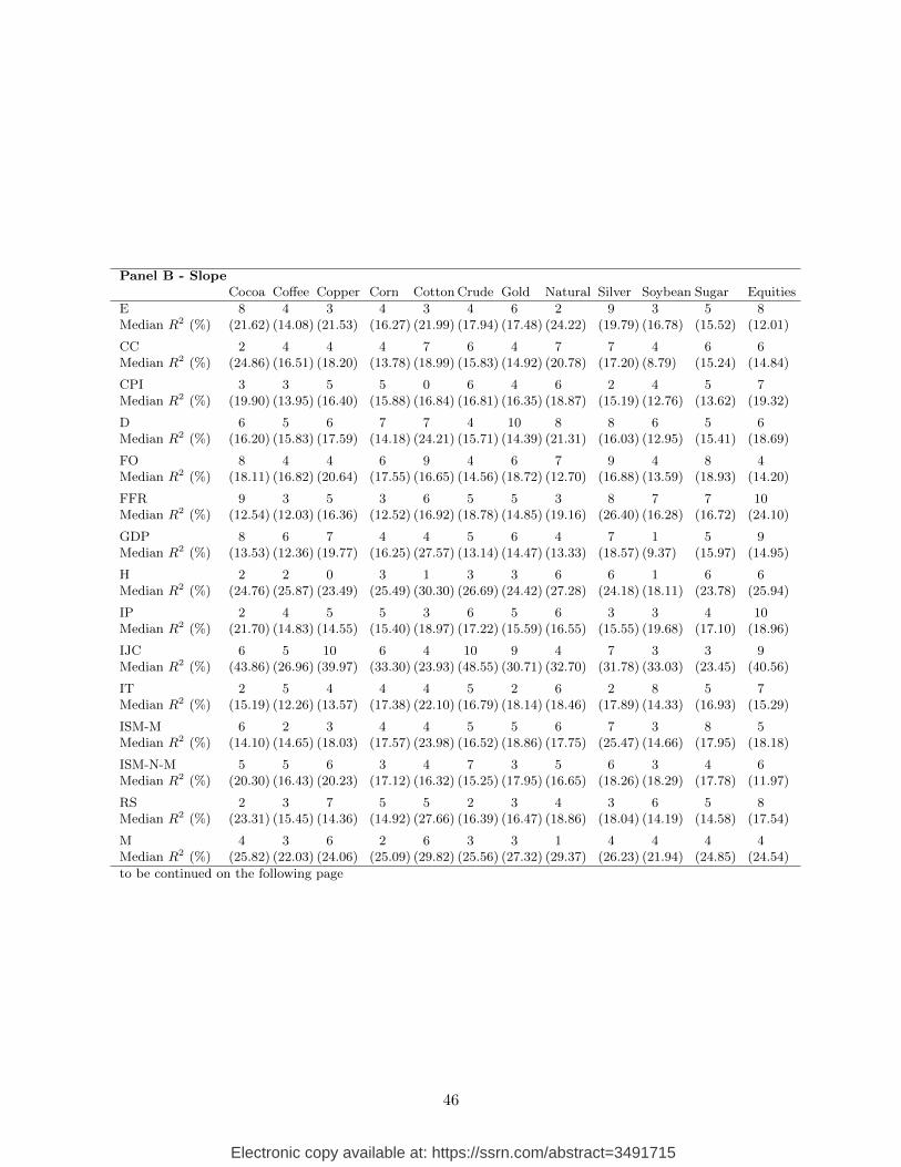
Panel B - SlopeCocoa Coffee Copper Corn Cotton Crude Gold Natural Silver Soybean Sugar Equities

E 8 4 3 4 3 4 6 2 9 3 5 8Median R2 (%) (21.62) (14.08) (21.53) (16.27) (21.99) (17.94) (17.48) (24.22) (19.79) (16.78) (15.52) (12.01)

CC 2 4 4 4 7 6 4 7 7 4 6 6Median R2 (%) (24.86) (16.51) (18.20) (13.78) (18.99) (15.83) (14.92) (20.78) (17.20) (8.79) (15.24) (14.84)

CPI 3 3 5 5 0 6 4 6 2 4 5 7Median R2 (%) (19.90) (13.95) (16.40) (15.88) (16.84) (16.81) (16.35) (18.87) (15.19) (12.76) (13.62) (19.32)

D 6 5 6 7 7 4 10 8 8 6 5 6Median R2 (%) (16.20) (15.83) (17.59) (14.18) (24.21) (15.71) (14.39) (21.31) (16.03) (12.95) (15.41) (18.69)

FO 8 4 4 6 9 4 6 7 9 4 8 4Median R2 (%) (18.11) (16.82) (20.64) (17.55) (16.65) (14.56) (18.72) (12.70) (16.88) (13.59) (18.93) (14.20)

FFR 9 3 5 3 6 5 5 3 8 7 7 10Median R2 (%) (12.54) (12.03) (16.36) (12.52) (16.92) (18.78) (14.85) (19.16) (26.40) (16.28) (16.72) (24.10)

GDP 8 6 7 4 4 5 6 4 7 1 5 9Median R2 (%) (13.53) (12.36) (19.77) (16.25) (27.57) (13.14) (14.47) (13.33) (18.57) (9.37) (15.97) (14.95)

H 2 2 0 3 1 3 3 6 6 1 6 6Median R2 (%) (24.76) (25.87) (23.49) (25.49) (30.30) (26.69) (24.42) (27.28) (24.18) (18.11) (23.78) (25.94)

IP 2 4 5 5 3 6 5 6 3 3 4 10Median R2 (%) (21.70) (14.83) (14.55) (15.40) (18.97) (17.22) (15.59) (16.55) (15.55) (19.68) (17.10) (18.96)

IJC 6 5 10 6 4 10 9 4 7 3 3 9Median R2 (%) (43.86) (26.96) (39.97) (33.30) (23.93) (48.55) (30.71) (32.70) (31.78) (33.03) (23.45) (40.56)

IT 2 5 4 4 4 5 2 6 2 8 5 7Median R2 (%) (15.19) (12.26) (13.57) (17.38) (22.10) (16.79) (18.14) (18.46) (17.89) (14.33) (16.93) (15.29)

ISM-M 6 2 3 4 4 5 5 6 7 3 8 5Median R2 (%) (14.10) (14.65) (18.03) (17.57) (23.98) (16.52) (18.86) (17.75) (25.47) (14.66) (17.95) (18.18)

ISM-N-M 5 5 6 3 4 7 3 5 6 3 4 6Median R2 (%) (20.30) (16.43) (20.23) (17.12) (16.32) (15.25) (17.95) (16.65) (18.26) (18.29) (17.78) (11.97)

RS 2 3 7 5 5 2 3 4 3 6 5 8Median R2 (%) (23.31) (15.45) (14.36) (14.92) (27.66) (16.39) (16.47) (18.86) (18.04) (14.19) (14.58) (17.54)

M 4 3 6 2 6 3 3 1 4 4 4 4Median R2 (%) (25.82) (22.03) (24.06) (25.09) (29.82) (25.56) (27.32) (29.37) (26.23) (21.94) (24.85) (24.54)


46


Panel C - CurvatureCocoa Coffee Copper Corn Cotton Crude Gold Natural Silver Soybean Sugar Equities

E 3 3 6 6 2 10 5 5 4 3 4 8Median R2 (%) (14.20) (14.19) (15.35) (13.35) (12.53) (19.97) (14.15) (17.24) (17.33) (11.17) (14.12) (20.18)CC 4 4 2 4 4 5 0 6 5 5 4 8Median R2 (%) (14.96) (16.25) (16.65) (14.22) (12.49) (19.40) (13.96) (15.40) (16.01) (12.23) (14.44) (17.23)CPI 5 4 6 2 2 4 1 5 6 5 2 7Median R2 (%) (13.88) (14.07) (15.19) (14.57) (13.22) (16.19) (17.29) (14.51) (14.57) (16.51) (13.30) (26.56)D 5 3 7 5 4 6 5 7 8 5 4 9Median R2 (%) (15.31) (10.76) (18.95) (14.71) (11.91) (18.73) (17.34) (13.32) (13.21) (15.76) (13.40) (18.18)FO 3 4 6 4 7 6 6 5 7 2 2 8Median R2 (%) (15.20) (16.23) (19.56) (13.04) (14.23) (24.47) (13.98) (16.07) (18.01) (9.43) (14.94) (21.99)FFR 6 4 4 7 4 6 2 3 4 5 3 7Median R2 (%) (10.70) (10.60) (18.03) (12.64) (7.69) (25.20) (16.45) (15.20) (13.69) (13.57) (11.35) (18.06)GDP 5 5 7 8 2 4 4 7 4 6 3 7Median R2 (%) (14.61) (14.25) (15.38) (10.09) (11.00) (19.29) (18.85) (15.42) (16.79) (17.04) (12.59) (17.50)H 2 2 1 3 3 7 2 4 3 5 1 2Median R2 (%) (25.63) (25.76) (27.69) (25.98) (23.06) (26.51) (24.30) (24.48) (20.94) (30.24) (25.90) (23.75)IP 4 3 3 4 2 6 3 3 3 6 1 2Median R2 (%) (13.98) (17.29) (18.17) (15.55) (13.64) (24.12) (21.59) (17.43) (18.69) (21.35) (16.83) (30.19)IJC 2 7 3 7 5 9 5 6 3 5 5 7Median R2 (%) (30.85) (46.24) (33.48) (21.71) (33.45) (61.06) (26.78) (57.82) (32.35) (12.87) (29.05) (51.28)IT 5 6 4 4 2 5 5 6 7 6 0 8Median R2 (%) (15.23) (17.60) (19.69) (15.45) (15.24) (24.43) (20.61) (16.67) (15.94) (17.52) (13.71) (22.55)ISM-M 3 3 4 2 2 1 3 8 4 3 3 4Median R2 (%) (13.27) (14.96) (14.98) (14.54) (13.87) (24.94) (23.46) (20.65) (14.07) (14.31) (14.48) (16.47)ISM-N-M 2 2 2 3 4 8 8 4 5 1 2 6Median R2 (%) (14.16) (16.03) (17.27) (15.29) (12.57) (20.59) (27.57) (19.08) (15.81) (11.34) (14.36) (26.75)RS 2 5 3 3 0 4 2 5 4 5 1 7Median R2 (%) (16.17) (18.38) (18.96) (17.76) (15.46) (24.59) (19.97) (20.08) (16.84) (20.67) (15.91) (25.71)M 5 2 1 5 1 5 3 7 4 6 1 5Median R2 (%) (22.37) (22.26) (25.16) (23.20) (21.06) (26.81) (25.14) (22.92) (23.10) (24.80) (24.18) (26.56)

47


Volatility Term Structures in Commodity Markets

Online Appendix

Section A1 presents the factor loadings of the assets and the 5% VaR. Section A2

presents the data sources used. Section A3 presents additional tables of the state-

dependent spillover test and the macroeconomic news transmission. Section A4 pro-

vides the results of the robustness section in the main analysis, using different levels

for the VaR index, a different volatility setup and a parametric decomposition of the

PCs.

48


A1 Figures

Cocoa

−0.

50.

00.

5

Volatility (Time−to−Maturity)

Fact

or L

oadi

ngs

VIX_1 VIX_2 VIX_3 VIX_6 VIX_9 VIX_12

Coffee

−0.

50.

00.

5


Fact

or L

oadi

ngs


Copper

−0.

50.

00.

5


Fact

or L

oadi

ngs


Corn

−0.

50.

00.

5


Fact

or L

oadi

ngs


Cotton

−0.

50.

00.

5


Fact

or L

oadi

ngs


Crude

−0.

50.

00.

5


Fact

or L

oadi

ngs


Figure A1. Principal Component Factor loadings This figure shows the factor loadings ofthe first three PCs for each commodity. The level factor uses a black line with circles as dots, theslope is presented by a blue line and a triangle and the curvature is an orange line with a plus.

49


Gold

−0.

50.

00.

5


Fact

or L

oadi

ngs


Natural Gas

−0.

50.

00.

5


Fact

or L

oadi

ngs


Silver

−0.

50.

00.

5


Fact

or L

oadi

ngs


Soybeans

−0.

50.

00.

5


Fact

or L

oadi

ngs


Sugar

−0.

50.

00.

5


Fact

or L

oadi

ngs


Equity

−1.

0−

0.5

0.0

0.5

1.0


Fact

or L

oadi

ngs


Continued Figure A1

50


2000 2005 2010 2015

−0.

04−

0.03

−0.

02−

0.01

Date

VaR

Figure A2. 5% Value at Risk (VaR) of an Equally Weighted Portfolio of All Commodi-ties The VaR estimation follows the estimation of Engle and Manganelli (2004). This estimationcaptures volatility clustering and can be constructed entirely out-of-sample.

51


A2 Data Sources

Table A1 Data Sources

This table presents the data sources. Panel A introduces the futures dataset. Panel B presents macroeconomic

variables as in Stock and Watson (2012). Panel C introduces the series of macroeconomic announcements. In Panel

B we indicate the transformation method for the time series. We present the transformation codes in Table A2. An

explanation for the numbers can be found in Table A2. Abbreviations are: St. Louis Federal Reserve Economic

Data (FRED), Commodity Futures Trading Commission (CFTC), Department of Energy (DOE), Intercontinental

Exchange (ICE), U.S. Department of Agriculture (USDA), U.S. Department of Labor (DOL), University of Michigan

(UM), Federal Reserve (FED), Archival FRED (ALFRED), Institute of Supply Management (ISM), United States

Census (Census), New York Mercantile Exchange (NYMEX), New York Commodity Exchange (COMEX), Chicago

Board of Trade (CBOT) and seasonally adjusted (SA).

Panel A Sector Symbol Commodity Exchange

Softs CC Cocoa ICEKC Coffee ICECT Cotton ICESB Sugar ICE

Metals HG Copper NYMEX/COMEXGC Gold NYMEX/COMEXSI Silver NYMEX

Energies CL WTI Crude Oil NYMEXNG Natural Gas NYMEX

Agricultural C Corn CBOTS Soybeans CBOT

Panel B Name T Source Description

GDP components Cons-Dur 5 FRED SACons-NonDur 5 FRED SACons-Serv 5 FRED SAExports 5 DatastreamImports 5 Datastream

Industrial IP: cons dble 5 FRED 2007=100, SAproduction IP: cons nondble 5 FRED 2007=100, SA

IP: bus eqpt 5 FRED 2007=100, SAIP: dble mats 5 FRED 2007=100, SAIP: nondble mats 5 FRED 2007=100, SAIP: mfg 5 FRED 2007=100, SAIP: fuels 5 FRED 2007=100, SANAPM prodn 1 FRED SA; Discontinued in 2016-05Capacity Util 1 FRED SA

Employment Emp: mining 5 FRED SAEmp: const 5 FRED SAEmp: dble gds 5 FRED SAEmp: nondbles 5 FRED SAEmp: services 5 FRED SAEmp: TTU 5 FRED SAEmp: wholesale 5 FRED SAEmp: retail 5 FRED SAEmp: FIRE 5 FRED SAEmp: Govt 5 FRED SAEmp: Hours 5 FRED 2002=100, SAAvg hrs 1 FRED SAOvertime: mfg 2 FRED SA

Consumer expectations Consumer expect 2 FRED 1966Q1=100


52


Name T Source Description

Housing HStarts: NE 4 FREDHStarts: MW 4 FREDHStarts: S 4 FREDHStarts: W 4 FRED

Unemployment U: all 2 FRED SArate U: mean 2 FRED SA

U: < 5 wks 5 FRED SAU: 5-14 wks 5 FRED SAU: 15+ wks 5 FRED SAU: 15-26 wks 5 FRED SAU: 27+ wks 5 FRED SA

Business PMI 1 FRED SAinventories NAPM new orders 1 FRED SA

NAPM vendor del 1 FRED SANAPM Invent 1 FRED SAOrders (ConsGoods) 5 FRED SAOrders (NDCap-Goods)

5 FRED SA

Prices CPI-core 6 FRED 1982-84=100; SAPCED 6 FRED 2009=100; SA

Money M1 6 FRED SAM2 6 FRED SAMB 6 FRED SAReserves tot. 6 FREDBUSLOANS 6 FRED SACons credit 6 FRED SA

Interest rates FedFunds 5 FRED3mo T-bill 5 FRED6mo T-bill 5 FRED

Wages AHE: const 5 FRED SAAHE: mfg 5 FRED SA

Exchange rates Ex rate: avg 5 FRED 1973-03=100Ex rate: Switz 5 FREDEx rate: Japan 5 FREDEx rate: UK 5 FREDEx rate: Canada 5 FRED

Stock prices S&P 500 5 Datastream 1973-03=100DJIA 5 Datastream

Financial ADS 1 FREDconditions Sentiment 1 FRED

Baltic Dry Index 1 FRED

Commodityvolatility

CRBSPOT 1 Datastream

Cocoa 073732, 083731 2 CFTC 1996-2016; Speculation from CFTC datasetCoffee 085691, 085692 2 CFTC 1996-2016; Speculation from CFTC datasetCotton 067651 2 CFTC 1996-2016; Speculation from CFTC datasetSugar 080732 2 CFTC 1996-2016; Speculation from CFTC datasetCorn 002601, 002602 2 CFTC 1996-2016; Speculation from CFTC datasetSoybeans 005601, 005602 2 CFTC 1996-2016; Speculation from CFTC datasetGold 088691, 088606 2 CFTC 1996-2016; Speculation from CFTC datasetSilver 084691, 084605 2 CFTC 1996-2016; Speculation from CFTC datasetCopper 085691, 085692 2 CFTC 1996-2016; Speculation from CFTC datasetNatural gas 023651 2 CFTC 1996-2016; Speculation from CFTC datasetCrude oil 067651 2 CFTC 1996-2016; Speculation from CFTC dataset

Inventory Cocoa 5 ICECocoa monthly total stocksfrom Jan 1986 until Dec 2016

Coffee 5 ICECoffee monthly total stocksfrom Nov 1996 until Dec 2016


53


Name T Source Description

Cotton 5 ICECotton month-end total stocksfrom Aug 2002 until Dec 2016

Sugar 5 USDASugar total quarterly stocksa

from March 1990 until Dec 2016

Corn 5 USDACorn total quarterly stocksa

from Dec 1987 until Dec 2016

Soybeans 5 USDASoybeans total quarterly stocksa

Dec 1980 until Dec 2016

Gold 5 COMEXGold total monthly stocks via Datastreamfrom July 2002 until Dec 2016

Silver 5 COMEXSilver total monthly stocks via Datastreamfrom July 2002 until Dec 2016

Copper 5 LMECopper monthly stocks in LME warehousesfrom Jan 1970 until Dec 2016

Natural gas 5 EIANatural Gas monthly stocksfrom Jan 1979 until Dec 2016

Crude oil 5 EIACrude Oil and Petroleum products month-end stocksfrom Jan 1990 until Dec 2016

VRP 1 Webpage3 Difference between the risk-neutral and objectiveexpectations of realized variance

Panel C

Employment Sit-uation Report

1 DOL https://www.bls.gov/bls/archived_sched.htm

Consumer Confi-dence Index

1 ConferenceBoard

https://www.conference-board.org/data/

consumerconfidence.cfm

CPI 1 DOL https://www.bls.gov/bls/archived_sched.htm

Durable Goods Advance Report onDurable Goods Man-ufacturers’ Shipments,Inventories, and Or-ders

1 Census https://www.census.gov/manufacturing/m3/

about_the_surveys/index.html

Factory Orders Manufacturers’ Ship-ments, Inventories,and Orders

1 Census https://www.census.gov/manufacturing/m3/

about_the_surveys/index.html

Federal FundsRate

1 FED https://www.federalreserve.gov/

monetarypolicy/fomccalendars.htm

GDPb 1 ALFRED https://alfred.stlouisfed.org/release?rid=

53

Housingc 1 Census https://www.census.gov/construction/nrs/

historical_data/historic_releases.html

Industrial Pro-duction

Industrial Productionand Capacity Utiliza-tion - G.17

1 FED https://www.federalreserve.gov/releases/

g17/release_dates.htm

Initial JoblessClaims

1 ALFRED https://alfred.stlouisfed.org/release/

downloaddates?rid=180

InternationalTrade

FT900: U.S. Interna-tional Trade in Goodsand Services

1 Census https://www.census.gov/foreign-trade/

Press-Release/ft900_index.html

ISM Manufactur-ing PMI

1 ISM https://www.instituteforsupplymanagement.

org/ISMReport/content.cfm?ItemNumber=

10745&SSO=1

ISM N-Mfg PMI 1 ISM https://www.instituteforsupplymanagement.

org/ISMReport/content.cfm?ItemNumber=

10745&SSO=1

Retail Salesd Monthly Retail Trade 1 Census https://www.census.gov/retail/mrts/

historic_releases.html

Michigan Con-sumer Sentimente

University of Michi-gan/Surveys of Con-sumers

1 UM https://data.sca.isr.umich.edu/

survey-info.php

aThe weekly grain series was discontinued in Aug 26 2014 by the USDA, the National Agricultural StatisticsService (NASS) issues a quarterly series instead.

bIncludes the advance, second estimate and final estimate.cIncludes residential construction and sales.dWe choose the later date, if the announcement is split on two dates.eIncludes both preliminary and final announcements.

54


https://www.bls.gov/bls/archived_sched.htm

https://www.conference-board.org/data/consumerconfidence.cfm

https://www.conference-board.org/data/consumerconfidence.cfm

https://www.bls.gov/bls/archived_sched.htm

https://www.census.gov/manufacturing/m3/about_the_surveys/index.html




https://www.federalreserve.gov/monetarypolicy/fomccalendars.htm

https://www.federalreserve.gov/monetarypolicy/fomccalendars.htm

https://alfred.stlouisfed.org/release?rid=53

https://alfred.stlouisfed.org/release?rid=53

https://www.census.gov/construction/nrs/historical_data/historic_releases.html

https://www.census.gov/construction/nrs/historical_data/historic_releases.html

https://www.federalreserve.gov/releases/g17/release_dates.htm

https://www.federalreserve.gov/releases/g17/release_dates.htm

https://alfred.stlouisfed.org/release/downloaddates?rid=180

https://alfred.stlouisfed.org/release/downloaddates?rid=180

https://www.census.gov/foreign-trade/Press-Release/ft900_index.html

https://www.census.gov/foreign-trade/Press-Release/ft900_index.html

https://www.instituteforsupplymanagement.org/ISMReport/content.cfm?ItemNumber=10745&SSO=1






https://www.census.gov/retail/mrts/historic_releases.html

https://www.census.gov/retail/mrts/historic_releases.html

https://data.sca.isr.umich.edu/survey-info.php

https://data.sca.isr.umich.edu/survey-info.php

Table A2 Data Handling

This table presents category codes and data transformations, following Stock and Watson (2012), presented in Table

A1. Zt denotes the raw series and Xt the transformed series.

Code Xt

1 Zt

2 Zt − Zt−1

3 (Zt − Zt−1) − (Zt−1 − Zt−2)4 ln(Zt)5 ln( Zt

Zt−1)

6 ln( ZtZt−1

) − ln(Zt−1

Zt−2)

55


A3 Additional Tables

Table A3 Spillovers Between Different Markets – Level Factor

This table presents in-sample and out-of-sample results for spillover tests for the level of the volatility term structure.

We run the following regression:

PCi,t =

p∑k=1


p∑k=1


p∑k=1


p∑u=1


p∑u=1


p∑u=1



spillovers originate) is presented in the first row. We test the null hypothesis, H0 : γ1u = 0 (H0 : γ2

u = 0, H0 : γ3u = 0)

for normal (tranquil, distressed) periods. For in-sample significance, we use a Wald test of the H0 using Newey and

West (1986) standard errors with 10 lags. ∗,∗∗ ,∗∗∗, respectively indicate significance for the 10%, 5% and 1% level,

respectively. For out-of-sample tests, we use an expanding window, initialized by 100 observations. We present the

out-of-sample R2 (R2 = 1 − MSEunMSEre

) in the body of the tables. Significant R2s based on McCracken (2007) test

statistics are printed in bold.

Panel A - Normal

Cocoa Coffee Copper Corn Cotton Crude Gold Natural Silver Soybean Sugar Equity

Cocoa 1.20∗∗ 0.10 0.94 1.63 0.67∗ 1.17 0.54 1.14 0.23 0.94 0.40∗∗

Coffee 0.47 0.12 0.30∗∗ 1.27 1.39 0.14 1.54 0.30 0.05 0.34 0.41Copper 1.00 0.14 0.52 0.46 0.75 0.96∗∗ 0.10 0.74∗∗ 0.46 0.82 0.42Corn 1.23 0.64 0.33 −0.04 0.58 0.77 0.40 0.92 0.39∗∗ 1.04 0.34Cotton 0.19 0.25 0.27 0.64∗∗ 0.48∗∗ 0.26 0.19 0.71 0.66∗∗ 0.76∗∗∗ 0.16Crude 0.30 0.52∗ 0.96 0.59 1.32 0.66 0.38 0.74 0.77 1.11 1.09∗

Gold 0.41∗∗ 0.34 0.84 0.57 0.81 0.60∗∗∗ 1.15 0.88 0.12 0.19 0.54∗∗∗

Natural 0.13 0.77∗ −0.16 1.33∗ 2.39∗∗ 0.46 −1.39 0.25 1.70 −0.18 0.52∗

Silver 0.40 0.27 0.85 0.44 0.65∗∗ 2.04∗∗∗ 0.60∗∗∗ 0.29∗∗∗ −0.10 0.61 0.80∗∗

Soybean 0.42∗∗∗ −0.23 1.06 0.63 1.09 0.58 0.42 1.66 0.07 0.44 0.31Sugar 0.68 0.13 0.33 0.91 0.98 1.49 0.24 0.09 0.77 0.15∗∗ 0.18Equity −0.05 −0.45∗ 0.20 0.10 −0.75∗∗ 0.39 0.11 0.62 0.65 0.15 0.24

Panel B - Tranquil


Cocoa 0.11 0.13 0.94 1.23∗∗∗ 1.57∗∗∗ 1.29∗∗∗ 0.25 0.22∗∗∗ 0.49 −0.10∗∗∗0.30∗∗∗

Coffee 0.68 0.11 0.32 0.63 1.10 0.13 0.63 −0.05∗∗∗0.55 0.49 0.04Copper 0.20∗∗∗ 0.20 0.28 0.20∗ 0.25∗ 0.29 0.20∗∗ 0.67∗∗∗ 0.59∗∗ 0.62 0.30Corn 0.53 0.17 0.40∗∗∗ 0.56 0.37∗∗∗ 0.50 0.00 0.85 0.20∗∗ −0.64∗∗∗0.26Cotton 0.17 0.21 0.30 0.16 0.39 0.14 0.92 0.47 0.30∗∗∗ 0.25∗∗ 0.11Crude 0.23 0.51∗∗∗ 0.21∗ 0.27 0.45 0.43∗∗∗ −0.92 0.24∗∗∗ 0.20∗∗ 0.17 0.48∗∗∗

Gold 0.49 0.10 0.26∗ 0.64 0.44∗∗∗ 0.63∗ 0.47 0.04 0.06 0.47 0.38∗∗∗

Natural 0.47 0.49 0.08 1.23∗∗ 1.34 0.26∗∗∗ −0.90 0.10 0.08∗∗ 0.45∗∗ 0.62∗∗

Silver 0.36∗ 0.61 0.54 1.38 0.68 0.59∗∗∗ 0.68∗∗ 0.68∗∗∗ 0.24 0.44 0.44∗∗

Soybean 0.34∗∗∗ 0.16∗ 0.40∗∗∗ 0.07 −0.41∗∗ 0.43∗ 0.18 0.07 0.15 0.22 0.22Sugar 0.06 0.20∗∗∗ 0.04 0.10 0.11∗ 0.11∗ 0.07 0.25∗∗∗ 0.13∗∗∗ 0.11 0.11∗∗∗

Equity 0.24∗∗∗ 0.28 −0.03∗∗∗0.05 −0.19∗∗∗0.49∗∗∗ −0.19∗ 0.29∗∗∗ 0.29∗∗∗ −0.32∗ 0.07∗∗∗

Panel C - Distressed


Cocoa 0.32∗∗∗ 1.23 0.89 1.56 0.87∗∗ 1.49 −0.59 1.25 0.65 0.79∗∗∗ 0.94∗

Coffee 0.14 0.37 0.76∗∗∗ 2.64 1.62 0.09 1.53 0.00 −0.37 0.39∗∗ 0.32Copper 1.05 0.22 0.50∗ 0.40 1.09∗ 1.59∗∗ 0.08 1.70∗∗∗ 0.44 0.68 0.94∗∗

Corn 1.83 1.17 0.61 −0.05 1.30 1.56∗ 1.27 1.46 1.02 1.47 0.47Cotton 0.32 0.60 0.89 0.74 0.86∗ 0.42 0.59 1.35 1.46∗∗ 0.64∗ 0.31Crude 0.32∗ 0.26 1.05 0.74 1.18 0.75 0.68∗ 0.72 1.54∗∗ 1.74 1.21∗∗∗

Gold 0.39∗∗ 0.45 1.56∗∗ 0.90 1.02∗ 0.37∗∗ 1.38 1.14 0.34 0.49 0.58∗∗

Natural −0.34 0.87 0.55∗∗∗ 2.34∗ 2.15∗ 0.24∗ −0.92 0.33 1.47 −0.14 −0.17∗∗∗

Silver 0.72 0.61 1.01 0.91 0.49∗ 1.28∗∗∗ 0.62∗∗∗ 0.30 0.09 0.82 1.17∗

Soybean 0.30 0.29 2.07 1.10 1.49 1.54 0.65 1.55 0.16∗ −0.01∗ 0.03∗∗

Sugar 0.69 0.08 −0.13 0.41 0.84 2.15 −0.56 0.18 0.93 −0.09 −0.36Equity −0.29 0.15 0.55 −0.13 −0.25 0.31 −0.16 0.19 1.15 0.34 −0.04

56


Table A4 Spillovers Between Different Markets – Slope Factor

This table presents in-sample and out-of-sample results for spillover tests for the slope of the volatility term structure.

We run the following regression:

PCi,t =

p∑k=1


p∑k=1


p∑k=1


p∑u=1


p∑u=1


p∑u=1




u = 0, H0 : γ3u = 0)







Panel A - Normal


Cocoa 0.27 0.31 −0.11 −0.74 −0.33∗∗ −1.37 0.05 0.65 −0.54∗∗ −0.29 −0.29Coffee 0.28 0.12 0.18 1.13 0.98∗∗ 0.30 0.97 −0.13 −0.15 0.55 0.07∗∗∗

Copper 0.05 0.27∗ −0.16 0.32∗∗ 0.30 0.72∗∗ 0.15∗ 0.87∗∗∗ 0.74 0.89 0.24∗∗

Corn 0.89∗∗∗ 1.68∗∗∗ 0.12 −0.05 0.96 1.06 2.33 −2.24∗∗ 0.62∗∗∗ 0.65∗∗ 0.29∗

Cotton 0.25∗∗∗ 0.78 0.29 0.44∗∗ −0.13 0.32 0.04 0.41 0.41∗∗ 1.54∗∗ 0.33Crude 0.94 0.15 0.60 0.46∗ 0.74 1.49 0.10∗∗ 0.24 0.14 0.04 0.15Gold 0.24 0.04 0.27 −0.29∗∗∗0.14 0.99∗∗∗ 1.38 1.78∗∗ 0.84∗∗ 0.48 0.30Natural 0.11 −1.59 −0.31 0.78 −0.90 0.91 1.68 0.01 −0.13 −0.48∗∗ 0.92∗∗

Silver 0.44 0.56 −0.10 0.07∗ 0.09 0.43 0.17∗∗∗ 0.01∗∗ 0.11 1.20 0.72∗∗

Soybean 0.46 1.77∗∗∗ 0.57 0.39∗∗ 0.53 0.48 −0.01∗ 1.35∗ 0.02∗ 0.16∗∗∗ 0.00Sugar 0.54∗∗ −0.11 0.17 0.37 0.38∗ 0.30 −0.42 0.10 1.48 −0.09 0.02Equity −2.67 −3.74 −1.35 −2.41∗ −1.94 −1.39∗∗∗−4.94∗∗∗−0.75 0.07 −0.47 −3.87

Panel B - Tranquil


Cocoa −0.11∗∗ −0.18∗∗ −0.37∗∗∗−0.76 −0.05∗∗∗−0.19 0.35∗∗∗ −0.26 0.14 −0.73 −0.11∗∗∗

Coffee 0.22∗∗∗ 0.09∗ −0.02∗∗ 0.43 0.02 0.02 0.75∗∗ 0.21 0.21∗∗ 0.07∗∗∗ 0.10∗∗∗

Copper 0.19 0.03∗∗ 0.09 0.03 0.05∗∗∗ 0.05 0.06∗ 0.14 −0.01 0.19 0.15Corn 0.11∗∗∗ −0.01 −0.64 −0.25∗∗∗−0.07∗∗∗−0.35∗∗ 0.84∗∗∗ 0.52∗ 1.62 −0.74 0.39∗∗∗

Cotton 0.16 0.20 0.37∗∗∗ 0.41∗∗ −0.05 0.49∗ 0.73∗∗∗ 0.36 −0.00 0.42∗∗∗ 0.29∗∗∗

Crude 0.41 0.25 0.06 0.45∗∗∗ 0.03 0.31∗∗ −0.43∗∗∗0.19 0.26 0.36∗∗ 0.80∗∗∗

Gold 0.18 −0.02 0.22 0.50∗∗∗ 0.39∗∗∗ 0.33∗∗∗ 0.36∗∗∗ 0.73∗∗ 0.42 0.50 0.56∗∗∗

Natural −1.06 −0.78∗ 0.05 −2.64∗ 2.02 −0.89∗∗∗−0.10 0.08 0.15 −1.90 −1.32∗∗∗

Silver 0.52∗∗∗ 0.28 0.33 0.23 0.54 −0.22∗∗∗−0.16 0.01 0.61 1.74 0.82∗∗∗

Soybean 0.01 0.18 0.09 0.53∗ 0.16∗∗ 0.19 0.25∗∗ 0.49 −0.05∗ 0.10 0.49∗∗

Sugar −0.01 0.09∗∗ −0.09∗∗∗−0.02 −0.05∗∗ −0.05∗∗∗−0.11∗∗ 0.15∗∗∗ 0.17∗ 0.08 −1.34∗∗∗

Equity −5.74 −1.77 0.05 −4.81 −6.26∗∗ 0.54∗∗∗ −8.10 −0.77∗∗∗−1.01∗∗∗0.48 −0.41∗

Panel C - Distress


Cocoa 0.34∗ 0.76 1.12∗∗ −0.27 −0.21 −1.38∗ −0.71 0.62 0.12 −1.72 −1.16Coffee 0.52∗ −0.31 1.07 2.50 2.24∗∗∗ 0.69 −0.21 −0.48 0.08 0.26∗ −0.19Copper 0.15 0.12∗∗ −0.08 0.55 0.21 1.13 0.02 0.69 −0.09 1.48 0.54Corn 1.15∗ 1.23∗∗∗ 1.12 0.25 1.37 1.66 3.00∗∗ −1.26 0.50∗∗∗ 0.34 0.56Cotton 0.05 0.70∗ 0.37 0.54∗∗ 0.55 0.56 0.52 0.06 0.61 1.03∗ 0.34Crude −0.11 0.05∗ 0.70∗∗ 1.84∗∗ 1.16∗ 0.67 0.55∗∗∗ 0.97 0.20∗ 0.08 −0.66∗∗∗

Gold 0.36 0.09 0.27 0.30 0.35 0.26 1.63 1.67 0.37 0.49∗∗ 0.33∗∗

Natural −0.14 −0.26 0.31 3.28 4.48 0.04 −0.38 −0.30 −4.16 0.25∗∗ −0.30∗

Silver 0.46 0.83∗ 0.23 0.15 0.13 0.46∗∗ 1.06∗∗ 0.58 −0.08 1.11 1.39∗∗∗

Soybean 0.19 0.55 0.43 0.84∗∗ 0.17 0.53∗ 0.45 0.30 0.04 0.61 0.60Sugar 0.83 −0.48 −2.74 0.32 1.70 0.38 −1.96∗∗∗0.15 0.69 0.17 −1.62Equity −3.99∗∗∗−1.94 −2.16 −6.16 −2.43 −1.92 −3.56 −2.07 0.85 0.17 −4.64∗∗

57


Table A5 Spillovers Between Different Markets – Curvature Factor

This table presents in-sample and out-of-sample results for spillover tests for the curvature of the volatility term

structure. We run the following regression:

PCi,t =

p∑k=1


p∑k=1


p∑k=1


p∑u=1


p∑u=1


p∑u=1




u = 0, H0 : γ3u = 0)







Panel A - Normal


Cocoa 0.09∗∗∗ 0.85 0.70∗∗∗ −0.37∗ 0.09∗∗ 0.24 −0.12∗∗∗1.79 0.56 1.93∗∗∗ 1.00∗∗∗

Coffee 0.19∗∗∗ 0.34 −0.09∗ 0.02 1.13 0.54 1.99∗∗ 1.00 0.06 −0.17∗∗∗0.06Copper 0.56∗ 0.07 0.36∗∗∗ 0.47∗∗ 0.19 0.50∗ 0.07 0.41 0.38 0.34 0.17Corn −0.01∗∗ 1.67 0.15 1.32∗∗ 0.31 0.05 1.49∗∗∗ −0.65 2.17 0.82∗∗ 0.22Cotton −0.06 0.36∗ 0.06 0.04 0.12 0.19∗∗∗ 0.28 0.36 0.08 0.37∗∗∗ 0.05Crude 0.14∗ 1.48 0.18 1.36 0.50 0.59 −0.00 −0.47 0.02 0.07 −0.35Gold −0.10 0.01 −0.01 0.15 −0.09 0.38∗∗ 0.36∗ −0.21∗ −0.16 0.39 0.14Natural 1.38∗∗∗ 0.16 −0.59 1.03∗∗∗ −0.27∗∗ −0.46 −0.24∗∗ 0.22∗ −0.12 −0.82 −0.13∗∗∗

Silver 0.22 −0.29∗∗∗0.65 0.03∗∗ −1.10 −0.11 0.06 0.30 0.35∗∗ 0.03 0.07Soybean −0.09 −0.04 0.50 0.54∗∗ 0.18 −0.12∗ 0.62 0.05 0.02 0.01 −0.10Sugar 0.52∗∗∗ 0.08 −2.80 0.51∗∗∗ 2.00 1.05 −3.94 0.11∗∗∗ 0.12∗∗ −2.34∗∗ −1.63Equity −1.93∗∗ −7.34 −2.81 −1.59 −0.58 −1.76 −2.82∗∗∗−1.22∗ −0.01 0.02∗∗∗ −2.82∗∗∗

Panel B - Tranquil


Cocoa 0.58∗∗ −0.13∗∗∗0.25∗ 0.19 −0.07∗ 0.04 −0.00 0.10 −0.19∗∗ 0.03 0.42∗∗∗

Coffee 0.05 0.26 −0.12 −0.27 0.14 0.12 0.07∗∗∗ 0.27 0.00∗∗∗ −0.11∗∗∗0.05∗∗∗

Copper 0.06∗∗∗ 0.21∗∗ −0.01∗∗∗0.27∗ 0.01 −0.30∗∗∗−0.00∗∗ −0.38 −0.18 0.43∗∗∗ 0.25∗∗

Corn 0.52∗ −0.20 −0.00∗∗∗ −0.01 −0.06 0.26 −0.02 −0.05 −0.28 −1.68∗∗∗0.39∗∗∗

Cotton 0.44 0.17∗∗ 0.29∗∗∗ 0.19∗ 0.49 0.08 0.40 0.91∗ 0.42∗∗ 1.09∗∗ 0.06∗∗

Crude 0.64 0.12 0.05∗∗∗ 0.18 0.20∗ 0.34 −0.66 −0.00∗ 0.02 −0.01 −0.48∗

Gold 0.08 0.01 0.04∗ 0.12 −0.20 −0.04∗∗ 0.10∗∗ 0.14∗ 0.89∗∗ 0.06 0.09∗∗∗

Natural −0.71∗∗∗1.41 −0.44 2.19∗ −1.30 −0.28 −1.75 0.18 1.73∗∗∗ 0.58 1.82∗∗∗

Silver −0.24 0.25∗ 0.48 0.40∗∗ 0.29∗∗∗ 0.17∗∗∗ 0.37∗∗∗ 0.74 −0.65 −0.14 0.14∗

Soybean −0.01∗∗ 0.05 0.08∗∗∗ 0.18∗∗ 0.09 0.03 −0.01 0.27 0.16∗∗∗ 0.10 0.27∗

Sugar −0.04∗∗∗0.07 0.10∗∗∗ −0.02∗∗∗−0.02 −0.18∗∗ 0.04 −0.04 0.34∗ 0.14 0.11∗∗

Equity −4.60∗∗ 0.79 −0.20∗∗∗−2.85 −3.68 0.01 −2.68 −0.58∗ −0.02∗∗ −1.90 −0.09∗∗∗

Panel C - Distress


Cocoa −0.80∗∗∗0.94 0.76∗∗∗ −0.39∗∗ 0.68 0.22 −0.05∗∗∗0.47∗∗ 0.61 2.02∗∗∗ 0.30∗∗

Coffee 0.32 0.18 0.61 1.80 2.03 0.19 1.56∗∗ 1.38∗∗∗ −0.08 0.09 −0.51Copper 0.46 0.01 0.65 0.56 0.27∗ 0.50 0.09 0.38 0.74 0.94 0.49Corn 1.97∗ 1.48 0.74 3.59∗∗ 0.49 1.00 2.14∗∗ 0.82 −0.65 0.45∗∗∗ 0.94∗∗

Cotton 0.72 0.64∗ 0.40∗∗ 0.04 0.62 0.35 0.33 1.33∗ 0.82 0.76 0.37Crude 0.48 0.18 0.09 1.73 0.36 −0.52 0.28∗∗ −0.53 −0.06 0.99 −0.65Gold 0.01 0.31 0.04 0.44 0.69 0.11 0.45 1.40∗ −0.07 0.15∗∗ 0.20∗∗

Natural 1.46 0.91 0.49∗∗ 1.65∗ 0.87∗ 0.55 0.99 0.22 0.20∗ 0.38 0.94Silver −0.10 −0.30∗∗∗0.23 0.05 −1.25 0.16 −0.08 0.57 0.23 −0.67 0.44Soybean 0.53 0.24 0.64 0.93∗∗∗ 1.69∗ 0.45∗ −0.04 1.08 0.94 0.08 −0.26Sugar 0.45 −0.55 −12.08 0.95∗∗ 4.24 1.70∗∗∗ −13.89 0.25 −0.57∗ 0.98∗∗∗ −10.35Equity −2.69 −1.52 −2.57 −2.69 −0.44 −2.80 −2.07∗ −1.23 −0.13 −0.29 −2.02

58


Table A6 State-Dependent Spillovers – Pre-Financialization


term structure, for the pre-financialization period. We run the following regression:

PCi,t =

p∑k=1


p∑k=1


p∑k=1


p∑u=1


p∑u=1


p∑u=1








) in the body



Cocoa 0.68 1.51 1.78 0.99 0.62 0.26 0.87 5.61∗∗∗ 7.82 1.61∗∗∗ 0.38∗∗

Coffee 3.08 2.11 0.78 2.83 1.22∗ 3.19 2.75 −0.15 2.28∗ 3.25 1.54Copper 2.28∗∗∗ 3.40 4.95 6.08∗∗ 2.50 4.43∗∗ 5.46∗∗∗ 2.44∗∗∗ 1.55 3.14 1.65∗

Corn 0.89 1.72∗ 2.39∗∗∗ 2.51 1.56 2.39 1.37 2.56 6.66∗∗ 3.17∗∗ 1.19Cotton 1.74 6.32 2.63 1.82 1.09 2.01∗∗ 5.81 2.72 0.31 1.71 1.83Crude 1.03 1.54 2.09∗∗ 1.30 3.87∗ 1.42 1.73∗∗ 3.39∗∗ 2.86 1.55∗ 2.26Gold 1.44∗∗∗ 2.77∗ 1.01 1.10 2.29 0.53 1.28 5.14∗∗ 2.95 0.75 1.56Natural 3.94 3.52 0.07 2.91 7.24 3.92 −1.79 3.16 2.43 3.03 3.22∗∗∗

Silver 2.03 0.10∗∗ 0.45 1.20∗∗ 2.60 0.69 2.34∗∗∗ 1.72∗∗∗ 3.91∗∗∗ −1.17∗ 3.45∗∗∗

Soybean 8.22∗∗∗ 7.80 3.80 1.78 −2.63 6.43∗∗∗ 5.46 4.66∗ 1.44∗ 4.59∗∗∗ 2.70Sugar 0.13 0.10∗∗∗ 0.40 1.36 −3.23 −0.58 −0.39∗∗∗9.96 4.65∗∗∗ 10.43 2.00∗∗∗

Equity −0.25 −0.34∗∗ −0.30 1.35 −0.07 0.51∗∗∗ −0.68∗ 0.11 0.82∗∗ 2.86 1.93


Cocoa 2.53∗∗ 1.67 3.55∗∗ 1.41 −0.43 0.49∗∗∗ −1.76∗∗∗−3.40 0.25 −1.30∗∗∗−0.46Coffee 2.02 2.34∗∗∗ 1.69 0.84 1.38 0.90 4.66∗∗∗ 6.57∗ 2.94 2.08 0.51Copper 0.16∗∗∗ 1.26 4.05∗ 2.19∗ 1.95 −0.59 3.77 2.59 2.14 3.41∗∗ 0.63∗∗∗

Corn 2.56∗∗ 6.01∗∗∗ 1.88 1.97 1.58 3.36∗∗∗ 4.62∗ 4.74∗∗∗ 5.73∗∗∗ 2.60 0.83Cotton 1.59 3.38 1.56 3.17∗∗∗ 4.00 1.92 5.28∗∗∗ 2.40∗∗ 3.48∗∗∗ 2.90 2.36Crude 1.61 0.96 2.00∗∗∗ 1.06∗∗∗ 2.04∗∗∗ 4.01∗∗∗ 0.54∗∗∗ −0.52 2.71 1.37∗ 1.75Gold 1.33∗∗ 3.07∗∗∗ 2.33∗∗∗ 1.71∗∗∗ 0.68 1.15∗∗∗ 2.66∗∗∗ 3.63 2.99∗∗∗ 2.38∗∗∗ 0.55Natural 1.36 0.44 0.14 0.91∗∗∗ 5.01 −0.54 3.55 0.78∗∗∗ 2.82 −0.00 −1.42∗∗∗

Silver 0.84∗∗∗ 3.05∗∗∗ 1.32 −0.04∗∗∗−1.23∗∗∗0.52∗∗ 2.91∗∗∗ 2.79∗∗∗ 3.21 3.57∗∗∗ 1.31∗∗∗

Soybean 0.94∗∗ 2.89∗∗∗ −0.29 3.36∗∗ 0.25 0.68 1.87 0.11 −1.67 4.70∗ 1.26Sugar −3.53 −0.97 0.06 −0.88∗∗ −11.77 −0.04 −2.46∗∗ −0.03∗ 4.87∗∗ 5.50 0.51Equity −4.21∗∗∗−4.09 −3.51∗∗∗−6.54 −2.68 −0.58∗∗∗−9.08∗∗∗−14.56 0.21 −2.74 −1.78


Cocoa 0.04∗∗∗ 2.06∗∗∗ 3.58∗∗∗ 2.82∗ 1.73∗ 1.74∗∗∗ 2.03∗∗∗ −1.73 3.55∗∗∗ 3.84∗∗∗ 0.40∗∗∗

Coffee 2.02∗∗ 0.53 0.77 0.37 0.38 1.94 2.09 2.87 −1.00 0.47 −0.18Copper 2.24 1.14 4.75∗∗∗ 2.26∗ 0.91 1.73 2.12∗∗∗ 2.95 3.79∗∗∗ 2.62∗∗∗ 0.62∗∗

Corn 3.49 4.34∗∗ 2.37 5.12∗∗ 4.99 2.71 6.10∗∗∗ −1.08 3.77∗∗∗ 4.18∗∗∗ 1.94Cotton 1.68 3.17∗∗ 2.45 1.50 3.82 0.67∗∗∗ 3.97 3.47 −0.05 4.64∗∗∗ 1.77Crude 0.51∗ −1.10 0.96 0.40 −0.08 0.08 0.35∗∗ 0.69 1.91 1.71 0.39∗

Gold 0.16∗∗ 1.01∗∗∗ −0.02 1.07 −0.40 0.44∗∗ 0.72∗ 0.76 0.22 −0.17 0.30∗∗∗

Natural 0.08 2.96 4.20 3.02 2.90 0.29 0.86 3.29 0.35∗ 1.09 1.47∗∗∗

Silver 3.48∗∗∗ −1.03∗∗∗1.68 3.77∗∗∗ −1.32∗∗ 1.67 2.02 1.55∗∗∗ 3.34∗∗∗ 4.49∗∗∗ 2.79∗∗∗

Soybean 0.96∗ 0.77 0.57 1.45 0.84∗∗∗ 0.76 1.50 1.94∗∗∗ 5.69∗∗∗ 4.48 0.86Sugar −9.83∗ 0.37 −6.93 4.20∗∗∗ −9.55∗∗ 2.36∗∗∗ −11.60 1.27∗∗∗ 4.44∗∗∗ 9.48∗∗ 0.13Equity −4.47 −3.15 −6.61 −6.76 −8.87 −8.73 −7.26 −9.32∗∗ −1.69 0.97 −8.74∗∗

59


Table A7 State-Dependent Spillovers – Post-Financialization


term structure, for the post-financialization period. We run the following regression:

PCi,t =

p∑k=1


p∑k=1


p∑k=1


p∑u=1


p∑u=1


p∑u=1








) in the body



Cocoa 1.47 0.84∗∗∗ 3.28∗∗∗ 2.93∗∗∗ 1.61 1.84∗∗ 1.78∗∗∗ 0.82 3.26∗∗∗ 3.08∗∗∗ 2.33∗∗∗

Coffee 1.70∗∗ 1.83 2.57∗∗ 1.69 2.06∗∗∗ 1.86∗∗∗ 2.47∗∗ 0.64∗∗ 1.06 2.26∗∗∗ 1.71∗∗∗

Copper 2.14∗∗∗ 0.77∗∗∗ 2.01∗∗∗ 1.83∗∗∗ 1.69∗∗∗ 2.29∗∗∗ 1.50∗∗∗ 1.88∗ 0.59∗∗∗ 1.13∗∗ 2.27∗∗∗

Corn 0.97 1.60∗∗∗ 0.81∗∗∗ 2.19∗∗∗ 2.11∗ 1.47∗ 0.93∗∗∗ 1.28 2.41∗∗∗ 1.30∗∗∗ 1.48Cotton 1.18 1.18 1.06∗∗ 2.50∗∗∗ 3.10∗∗∗ 1.97 0.51∗∗ 2.19 0.64∗ 2.84∗∗∗ 1.73∗∗∗

Crude 3.21∗∗∗ 2.16∗∗∗ 2.37∗∗ 0.97∗∗ 2.74∗∗∗ 2.81∗∗∗ 1.21 3.06∗∗∗ 2.45∗∗∗ 2.40∗∗∗ 2.32∗∗∗

Gold 2.14∗∗∗ 1.94∗∗ 2.52∗∗∗ 2.27∗∗∗ 1.77∗∗∗ 3.22∗∗∗ 1.43∗∗ 2.01∗∗∗ 1.98∗∗∗ 2.01∗ 2.81∗∗∗

Natural 0.96∗∗∗ 2.71∗∗ 0.94∗∗∗ 3.27 1.38∗∗ 1.11∗∗∗ 1.70 2.15∗∗ 1.57∗∗∗ 1.53 1.09∗

Silver 1.27∗∗ 1.86 1.69∗∗∗ 1.55∗∗∗ 1.69∗∗∗ 2.49∗∗∗ 3.93∗∗∗ 0.88∗∗∗ 0.68 2.74∗∗ 2.43∗∗∗

Soybean 0.95∗∗∗ 0.55 1.94∗ 1.50∗∗∗ 1.19 1.70 1.10∗∗∗ 0.63∗ 0.80 1.75∗∗ 0.93Sugar 1.82∗∗∗ 1.88 3.16 4.71∗∗∗ 1.32∗∗∗ 1.95∗∗∗ 2.03∗∗∗ 1.87∗∗∗ 1.86 2.44 1.80∗∗∗

Equity 0.67 0.52∗∗ 1.64 0.34 0.50∗∗∗ 1.51∗∗ 1.91∗ −0.56∗ 0.44∗∗∗ 0.70 1.51


Cocoa 0.48∗∗∗ 0.92∗ 0.01∗ 0.84∗∗ 1.63∗∗∗ 1.14∗∗∗ 1.02∗ 0.37 1.02 2.04∗∗∗ 0.75∗∗∗

Coffee 2.13∗∗∗ 1.83∗∗∗ 2.57 0.88∗∗∗ 2.50∗∗∗ 2.06∗∗∗ 3.06∗∗∗ 2.70∗∗∗ 1.30 2.82∗∗∗ 1.25∗∗∗

Copper 0.94∗∗ 0.33 0.86∗ 0.73 1.66∗∗ 2.41 0.98∗ 0.53∗∗ 2.12∗ −0.13 1.52∗∗∗

Corn 0.52∗∗∗ 2.18∗∗∗ 0.29∗∗∗ 0.56∗∗∗ 2.10∗∗∗ 0.84∗∗∗ −0.06∗ 1.54∗∗∗ 2.12∗∗∗ 2.26∗∗∗ 1.17∗∗∗

Cotton 0.98∗∗ 1.09 1.03∗∗ 1.51∗∗ 2.36∗∗∗ 2.95∗∗∗ 0.89 2.62 0.93 1.99∗∗∗ 1.44∗∗∗

Crude 0.96 1.77 0.79 1.06∗∗∗ 0.72∗∗ 1.79∗ 0.70∗∗∗ 1.83∗∗∗ 0.97 1.06 1.41∗∗∗

Gold 0.72∗ 0.44∗ 0.54 1.34∗ 0.60∗∗ 2.46∗∗∗ 0.61 1.64 0.20 1.76∗∗∗ 2.95∗∗∗

Natural 1.61∗∗ 0.71∗∗ 0.34∗∗ 1.78∗∗∗ 0.75∗∗ 2.71∗∗∗ −0.00∗∗∗ 2.59∗∗∗ 1.09∗∗∗ −0.26∗∗∗0.58∗∗∗

Silver 0.71 0.77∗ 1.45 1.35∗∗∗ 1.77∗ 2.43∗∗∗ 2.19∗∗ 1.01 0.08 1.50∗∗∗ 2.19∗∗∗

Soybean 1.41 1.48∗∗∗ 1.48∗∗∗ 1.41∗∗∗ 0.93 1.28∗∗∗ 2.88∗∗∗ 1.29 1.27 1.61∗∗ 2.37∗∗∗

Sugar 0.86 2.06∗∗ 4.40∗∗ −0.52∗∗∗2.14 6.05∗∗∗ 6.66 0.74∗∗∗ 7.32∗∗∗ 0.83 4.65Equity 1.08 −0.57 −2.19∗∗ −0.47 −0.66∗∗∗0.34∗∗∗ 0.07∗∗∗ −1.55 −3.33 −0.89 0.60∗∗


Cocoa 1.40∗∗∗ 0.61∗∗∗ 1.61∗∗∗ 1.04∗∗ 1.66∗∗∗ 0.42 1.93∗∗∗ 2.86∗∗∗ 1.28∗∗∗ 2.02∗∗∗ 0.09∗∗∗

Coffee 0.22 0.84∗∗∗ 0.60∗∗∗ 2.04∗∗∗ 0.64∗∗ 0.79∗∗ 0.79∗∗ 1.31∗∗∗ 1.24∗∗∗ 0.58∗∗∗ 1.24∗∗∗

Copper 2.43∗ 0.58∗∗∗ 1.41∗∗ 2.12∗∗ 0.92∗ −0.31 0.25 −0.01∗∗ 3.88 2.41 0.43∗∗

Corn 4.03∗∗∗ 0.82∗∗∗ 1.22∗∗∗ 1.69∗∗∗ 1.96∗∗∗ 1.22 1.65∗∗ 0.03∗∗∗ −0.06∗∗∗4.99∗∗∗ 1.56∗∗∗

Cotton 0.92 1.34∗∗∗ 0.82∗∗∗ 0.85∗∗∗ 0.69∗∗ 1.18∗∗∗ 0.48 1.00∗∗∗ 1.67∗∗∗ 1.75∗∗∗ 0.70∗∗∗

Crude 0.62 0.06 0.55 1.05∗∗ 0.68 1.04∗∗∗ 0.50 0.25∗∗∗ 0.68∗∗∗ 0.85 −0.13∗∗∗

Gold 0.66∗∗ 0.37 0.83∗∗∗ 0.38 1.69 0.39∗∗∗ 0.95 1.98∗∗∗ 0.76∗ 1.40∗∗∗ 3.59∗∗∗

Natural 2.65∗∗∗ 0.84∗∗∗ 0.83∗∗ 2.18∗ 0.09 1.47∗∗∗ 1.00 2.54 1.61∗∗∗ 1.91∗∗∗ 0.86∗∗∗

Silver 0.73 0.70 1.30 0.69∗∗∗ 0.50∗∗ 1.95∗∗∗ 0.64 1.11 1.13∗∗∗ 1.46∗ 1.99∗∗∗

Soybean −0.04 −0.00 0.91∗∗∗ 0.33∗∗∗ 0.34∗ 1.61∗∗∗ 2.74∗∗ −0.27 1.57 1.94∗∗ −0.76∗∗∗

Sugar 2.52∗∗∗ 1.20∗∗ 1.26∗∗ 1.02∗∗∗ 1.35 1.96∗∗∗ 2.68∗∗∗ 0.93∗∗∗ 2.68∗∗∗ 0.37∗∗∗ 1.32∗∗∗

Equity −2.03∗∗∗−2.14 −1.50 −0.31∗∗ −1.79 −0.96∗∗∗−1.32∗∗∗−0.80 −3.63∗∗∗−1.96∗∗∗−1.72∗∗∗

60


Tab

leA

8M

acro

econ

omic

New

sA

nn

oun

cem

ents

This

table

pre

sents

the

per

centa

ge

over

lap

bet

wee

nnew

sannounce

men

tdate

sof

diff

eren

tm

acr

oec

onom

icse

ries

.W

euse

the

abbre

via

tions

inth

ehori

zonta

lth

at

are

defi

ned

inth

efirs

tco

lum

nof

the

table

. ECC

CPI

DFO

FFR

GDP

HIP

IJC

IT

ISM

-MIS

M-N

-MRS

M

Em

plo

ym

ent

(E)

100

00

015

01

00

04

912

111

Consu

mer

Confiden

ce(C

C)

0100

114

04

314

00

00

00

0C

PI

01

100

00

62

22

33

86

00

13

17

Dura

ble

(D)

014

0100

04

538

011

00

00

12

Fact

ory

Ord

ers

(FO

)16

00

0100

33

00

81

130

07

Fed

eral

Funds

Rate

(FF

R)

05

85

4100

818

31

63

56

1G

DP

13

15

35

100

91

13

02

20

31

Housi

ng

(H)

07

11

19

07

5100

11

60

01

310

Indust

rial

Pro

duct

ion

(IP

)0

033

00

21

21

100

32

00

15

30

Init

ial

Joble

ssC

laim

s(I

JC

)0

06

86

110

82

100

93

55

3In

tern

ati

onal

Tra

de

(IT

)4

06

01

50

12

13

100

05

414

ISM

Manufa

cturi

ng

PM

I(I

SM

-M)

90

00

12

20

05

0100

00

9IS

M-N

-Mfg

PM

I(I

SM

N-M

)12

00

030

42

10

85

0100

01

Ret

ail

Sale

s(R

S)

10

13

00

50

615

74

00

100

24

Mic

hig

an

Consu

mer

Sen

tim

ent

(M)

60

86

30

18

10

15

27

41

12

100

Obs.

239

240

240

238

236

190

279

477

240

346

238

240

240

239

479

In%

of

the

sam

ple

4.7

84.8

04.8

04.7

64.7

23.8

05.5

89.5

54.8

06.9

34.7

64.8

04.8

04.7

89.5

9

61


A4 Robustness

Table A9 Summary Statistics SVIX Term Structure

This table presents the summary statistics for the SVIX option-implied volatility term structure. It shows the annu-

alized model-free estimate of option-implied volatility for the commodity market for monthly and annual volatilities.

The SVIX is seasonally adjusted via a trigonometric function. The sample starts from 1996 through 2015. V ol1 is the

one-month volatility, V ol12 is the twelve-month volatility. The column sd presents the standard deviation, 10%, 15%

and 90% denote the respective percentiles of the distribution. Finally AR(1) reports the first-order AR coefficient

(in percentage points).

mean sd 10% 50% 90% AR(1)

CocoaVol1 0.34 0.10 0.21 0.33 0.46 95.05Vol12 0.31 0.08 0.22 0.30 0.41 98.58

CoffeeVol1 0.43 0.15 0.27 0.41 0.63 96.33Vol12 0.41 0.11 0.29 0.40 0.56 98.56

CopperVol1 0.31 0.11 0.19 0.30 0.43 95.55Vol12 0.28 0.11 0.18 0.24 0.41 99.23

CornVol1 0.29 0.12 0.16 0.28 0.43 91.76Vol12 0.27 0.07 0.19 0.26 0.38 96.57

CottonVol1 0.27 0.10 0.18 0.25 0.40 97.28Vol12 0.24 0.07 0.16 0.22 0.34 99.10

Crude OilVol1 0.36 0.14 0.22 0.34 0.49 97.95Vol12 0.29 0.09 0.18 0.28 0.38 96.99

GoldVol1 0.18 0.07 0.10 0.17 0.26 97.80Vol12 0.19 0.07 0.10 0.18 0.29 99.77

Natural GasVol1 0.51 0.17 0.32 0.49 0.73 97.48Vol12 0.38 0.11 0.26 0.37 0.50 93.58

SilverVol1 0.31 0.12 0.19 0.29 0.44 97.82Vol12 0.31 0.12 0.19 0.31 0.46 99.75

SoybeansVol1 0.24 0.09 0.15 0.23 0.36 95.92Vol12 0.25 0.08 0.18 0.23 0.38 97.77

SugarVol1 0.37 0.13 0.23 0.36 0.54 96.48Vol12 0.28 0.08 0.19 0.27 0.39 98.58

EquityVol1 0.21 0.08 0.12 0.19 0.31 92.58Vol12 0.21 0.05 0.15 0.20 0.27 99.40

62


Table A10 State-Dependent Out-Of-Sample R2 SVIX

This table presents in-sample and out-of-sample results for spillover tests for the different components of the SVIX


PCi,t =

p∑k=1


p∑k=1


p∑k=1


p∑u=1


p∑u=1


p∑u=1








) in the body



Cocoa 0.63 2.32 2.09 3.08∗∗∗ 2.77∗∗∗ 5.58∗∗∗ −0.92 1.97∗∗∗ 1.01 2.19∗∗∗ 2.57∗∗∗

Coffee 1.74 0.70∗∗∗ 1.78∗ 3.21 3.53∗∗∗ 0.04∗∗∗ 3.38∗ 1.78∗ 0.90 0.77∗∗ 0.98∗∗∗

Copper 1.61∗∗∗ 0.60 1.17∗∗ 0.88∗∗∗ 1.84∗∗∗ 2.66∗∗∗ 0.44 2.90∗∗∗ 1.49∗ 1.48∗∗ 2.72∗∗∗

Corn 1.98∗∗ 1.57 0.67∗∗∗ −0.26∗∗ 1.64∗∗∗ 2.05∗∗ 1.77∗∗ 2.35∗∗∗ 1.88∗∗ 1.71 1.36Cotton 0.85 0.96 1.09 1.23 1.13∗∗ 0.65 1.63 2.53 2.37∗∗∗ 1.49∗ 0.64Crude 0.89∗ 1.10∗∗∗ 2.17∗∗∗ 1.45∗ 2.23∗∗∗ 2.34∗∗∗ 0.23 1.89∗∗∗ 2.07∗∗∗ 2.14∗∗ 2.70∗∗∗

Gold 1.35∗∗∗ 0.86 1.38∗∗∗ 1.54∗ 1.87∗∗∗ 2.70∗∗∗ 2.17 4.12∗∗∗ 1.33∗∗ 1.38∗∗∗ 2.28∗∗∗

Natural 0.99∗∗∗ 2.59∗∗ 0.68∗ 2.51∗∗ 6.94∗∗∗ 1.39∗∗ 2.33∗∗∗ 1.22∗∗∗ 2.39 0.34∗∗∗ 2.11∗∗∗

Silver 1.55∗∗ 1.13 2.22∗∗∗ 1.87∗∗ 1.00∗∗∗ 2.69∗∗∗ 3.11∗∗∗ 1.40∗∗∗ 0.05 1.65 2.91∗∗∗

Soybean 1.09∗∗∗ 0.72∗∗∗ 2.77∗∗∗ 1.42∗∗ 1.20∗ 1.97∗∗ 1.51∗∗∗ 3.20∗∗ 0.60∗∗∗ 0.51∗∗∗ 1.22Sugar 0.95 0.41∗∗∗ 0.30 1.42∗∗∗ 1.76∗∗∗ 5.60∗∗∗ 0.25 0.37∗∗∗ 1.18∗∗∗ 0.17 −0.06∗∗∗

Equity 0.73∗∗∗ 0.81∗∗∗ 1.77∗∗∗ 1.04 0.88∗∗∗ 1.61∗∗∗ 0.72∗∗∗ 0.96∗∗∗ 2.93∗∗∗ 0.17 0.94∗∗∗


Cocoa −0.72∗ 4.07∗∗∗ 0.78∗∗∗ −1.54 1.31∗∗∗ 2.97 −0.01∗∗∗3.00 1.12∗∗∗ −1.24 1.14∗∗∗

Coffee 0.25∗∗∗ −0.31∗ 1.29∗∗∗ 3.19 3.87∗∗∗ 1.21 0.69∗∗∗ 1.97 0.68 0.48∗ 0.52∗∗∗

Copper 0.81∗∗∗ 0.47∗ −0.05 0.62 0.19∗∗∗ 1.95∗∗∗ 0.05∗∗∗ 0.50∗∗∗ 1.20∗ 1.99 1.82∗∗∗

Corn −0.32∗∗∗2.15∗∗∗ 1.05 0.79∗∗ 1.25∗∗∗ 1.02 4.00∗∗∗ −2.47 0.70∗∗∗ −0.86 0.54Cotton 0.98 1.09 0.54∗∗∗ 1.25∗∗∗ 0.52∗∗∗ 0.84 0.78∗∗∗ 1.51 1.85∗ 2.84∗∗ 0.39Crude 0.99∗ 0.65∗ 1.47 2.18∗∗∗ 0.91 2.54 0.53∗∗∗ 2.01 0.81∗ −0.26 0.44∗∗∗

Gold 1.30∗∗∗ 0.31 1.06 0.42∗∗∗ 0.72∗∗∗ 1.99∗∗∗ 2.27∗∗∗ 3.58∗∗∗ 2.09∗ 1.16 0.76∗∗

Natural −0.99 0.14 0.72 0.63∗∗∗ 1.61 1.83∗ 1.91 0.42∗ −2.12 −0.34∗ −1.64Silver 0.11∗∗ 1.05∗∗ −0.48 0.91∗ −1.08 0.22∗∗∗ 0.93∗∗∗ 0.32∗∗∗ −0.40∗∗∗1.15∗∗∗ 2.14∗∗∗

Soybean 1.23 1.38∗∗∗ 1.35 1.10∗∗∗ 1.17 1.85∗∗∗ 1.81∗∗∗ 1.45∗∗∗ 0.14 0.67∗∗∗ 0.60Sugar 1.39∗∗ −0.02 −3.32∗∗∗−0.25∗∗∗2.14∗∗∗ 0.45∗∗∗ −0.13∗∗∗0.28∗∗∗ 1.26∗∗ 0.37 −0.93∗∗

Equity −3.79∗∗∗−1.37 −1.23∗∗∗−0.48∗∗ −1.56∗∗∗0.72∗∗∗ −3.01∗∗∗−0.47∗∗∗0.34∗∗∗ −6.29 −1.14


Cocoa −0.42∗∗∗1.56∗∗∗ 1.74∗∗∗ −0.94∗∗ 1.73∗∗∗ 1.09 −0.46∗∗∗1.07 −0.33∗∗∗2.93∗∗∗ 1.87∗∗∗

Coffee 1.20 −0.28∗∗∗−0.24∗∗ 2.34∗∗ 1.82 0.58 0.36∗∗∗ 4.36∗ 2.37∗∗∗ −0.60∗∗ −0.04∗∗∗

Copper 1.22∗∗∗ 0.33∗∗∗ 0.60∗∗∗ 1.06∗∗ 0.62∗∗∗ 0.98∗∗∗ 0.16 0.19∗ 0.22∗∗∗ 1.81∗∗∗ 1.08Corn 2.57∗∗∗ 2.39∗∗ 2.30∗∗∗ 2.44∗∗ 0.95∗∗∗ 0.24 3.91∗∗∗ 3.37 1.11∗∗∗ 1.53∗∗∗ 1.15∗

Cotton 1.33 0.82∗ 0.59∗∗∗ 0.36 0.95∗∗∗ 1.08∗∗ 0.84 2.12∗ 2.86∗∗∗ 2.52∗ 0.30Crude 1.41 1.44 0.39∗∗∗ 2.30 1.16 −0.44 0.35 −0.18∗ −0.12∗∗∗−0.10∗∗ −1.65∗∗∗

Gold 0.04 0.64 −0.14 0.60 0.38 0.07∗∗∗ 0.48∗∗∗ 0.24 3.11∗∗∗ 1.03∗ 0.26Natural 1.24∗ 2.39 −0.34∗∗∗4.69∗∗∗ 5.83 1.32 0.65 0.75 3.26∗∗∗ 0.41 1.84Silver −0.48 −0.55∗∗∗0.92 0.11∗∗ −2.26∗∗ −0.71∗∗∗0.51∗∗∗ 0.98∗∗∗ 0.07 −0.09 0.01Soybean 3.23 2.15 3.10∗∗∗ 1.87∗∗∗ 3.79 1.31∗∗ 2.50 2.69∗ 0.80 0.03∗∗ 1.69Sugar −0.71∗∗∗−0.38 −17.28∗∗∗0.05∗∗∗ 7.18 2.46 −22.43 −0.11∗∗∗0.21∗ −1.84∗∗∗ −14.89Equity −3.00 −1.35∗∗ −2.03∗∗∗−0.89∗∗ −0.32 −4.38∗∗∗−4.11∗∗∗−1.28 −0.34∗∗∗−9.43∗∗∗−3.67∗

63


Table A11 State-Dependent Out-Of-Sample R2 Parametric

This table presents in-sample and out-of-sample results for spillover tests for the different components of the implied

volatility term structure. We define the implied volatility term structure with a parametric definition, the level

V IX1,...,12, the slope V IX1 −V IX12 and the curvature −V IX1 + 2V IX6 −V IX12. We run the following regression:

PCi,t =

p∑k=1


p∑k=1


p∑k=1


p∑u=1


p∑u=1


p∑u=1








) in the body



Cocoa 1.21∗∗ 0.98 2.31∗ 2.92∗∗∗ 2.66∗∗∗ 3.75∗∗∗ 0.39∗∗∗ 1.99∗∗∗ 0.99 1.70∗∗∗ 1.63∗∗∗

Coffee 1.52 0.62 1.87∗ 3.68 3.12∗ 0.39∗∗ 3.04∗ 1.20∗∗∗ 0.90 0.91 0.72Copper 1.44∗∗∗ 0.43 1.43∗ 0.75 1.89∗∗∗ 2.58∗∗∗ 0.45 3.60∗∗∗ 1.35∗ 1.74∗∗ 2.12∗∗∗

Corn 2.14 1.51 0.87∗∗ 0.28 1.80∗∗∗ 1.83∗∗ 1.85 1.92∗∗∗ 1.58∗∗∗ 0.47∗∗∗ 1.40∗

Cotton 0.82 0.97 1.36 1.21 1.41∗ 0.98 1.92 2.58 2.00∗∗∗ 2.45∗∗ 0.56Crude 0.97∗∗ 1.26∗∗∗ 2.14∗∗∗ 1.42 2.40∗∗ 2.12∗∗∗ 0.40 2.03∗∗∗ 2.47∗∗∗ 1.95∗ 2.83∗∗∗

Gold 1.25∗∗∗ 1.00∗∗∗ 2.60∗∗∗ 1.65∗∗ 2.06∗∗∗ 2.07∗∗∗ 3.37 3.26∗∗∗ 1.35∗∗ 1.30∗∗∗ 1.54∗∗∗

Natural 0.82 2.86∗ 0.37∗∗∗ 2.95∗∗∗ 6.99∗∗∗ 1.34∗∗∗ 1.09 1.29∗∗∗ 1.91∗∗ 0.39∗ 1.31∗∗∗

Silver 1.46∗ 1.47 2.20∗∗∗ 2.69∗∗ 1.27∗∗∗ 3.84∗∗∗ 2.68∗∗∗ 1.30∗∗∗ 0.14 1.69 2.81∗∗∗

Soybean 0.93∗∗∗ 0.58∗∗∗ 2.98∗∗∗ 1.28∗ 1.13∗ 2.41∗∗∗ 1.24∗∗ 3.61∗∗ 0.59∗∗∗ 0.61∗∗∗ 0.28∗

Sugar 1.30 0.43∗∗∗ 0.96 3.02∗∗ 1.34∗∗∗ 4.17∗∗∗ 0.84∗∗ 0.37∗∗∗ 1.43∗∗∗ 0.23 0.62Equity −1.14∗∗∗−0.77∗∗∗1.61∗∗∗ −0.03 −0.70∗∗∗1.95∗∗∗ −0.36∗∗∗0.99∗∗∗ 2.79∗∗∗ 0.03 −0.14∗∗∗


Cocoa −0.14∗∗ 1.42 1.01∗∗∗ 0.74∗∗ −1.61∗∗∗−1.68 −1.36 1.17 −0.26 −2.95 −2.35∗∗∗

Coffee 0.94∗∗ −0.23 1.62 2.23 3.97∗∗∗ 1.03 1.27∗∗∗ 0.60 0.60 0.73∗∗∗ −0.21∗∗∗

Copper 0.67∗∗ 0.13∗∗∗ −0.07 0.42∗∗ 0.77∗∗∗ 1.56∗∗ 0.29 0.83∗∗∗ 0.30∗ 1.62 1.08Corn 0.92∗ 2.69∗∗∗ 0.04 1.06∗ 1.23∗∗∗ 1.02 4.24∗∗ −0.73∗∗ 1.42∗∗∗ −0.12∗∗∗0.50∗∗∗

Cotton 0.97∗∗∗ 0.28∗∗∗ 0.61∗∗∗ 1.54∗∗∗ 0.51 0.88∗ 0.33 1.65 0.84 2.81∗∗∗ 0.80∗∗∗

Crude 0.63∗∗∗ 0.66 1.37∗∗∗ 0.59∗∗∗ 1.18 1.00∗∗∗ 0.22∗ 2.56∗∗∗ 0.43 0.40 1.37∗∗∗

Gold 0.75∗∗∗ 0.34∗ 0.87 0.96∗∗∗ 1.01∗∗ 2.02∗∗∗ 2.79∗ 2.32∗∗∗ 2.28 1.25∗∗∗ 1.05∗∗∗

Natural 0.17 0.97 0.54 2.54 3.73 0.78 1.16 0.10 −0.58 0.38∗∗∗ −0.17∗∗∗

Silver 1.44 1.25 0.68 0.86 1.46 1.47∗∗∗ 1.38∗∗ 0.37∗∗∗ −0.63 2.57∗ 2.13∗∗∗

Soybean 0.40 0.97∗ 1.39 1.45∗∗ 0.69 0.92∗∗ 0.91∗ 1.98 0.27 0.47 0.53∗∗

Sugar 0.38 0.20∗∗∗ −0.21∗∗∗1.45∗ 1.90∗∗∗ 2.07∗∗∗ 0.59∗∗∗ 0.21∗∗∗ 2.13∗∗∗ 0.33 0.18Equity −7.76∗∗∗−5.94 −2.57∗∗∗−4.68 −5.04∗ −3.09∗∗∗−13.22∗∗∗−2.90∗∗∗0.73∗∗∗ −1.74 −5.57∗∗∗


Cocoa 1.15∗∗∗ 0.22∗∗∗ 0.19∗∗∗ −0.12 0.06∗∗∗ −0.29 1.57∗∗∗ 1.44∗∗ 0.65∗ −1.26∗∗ −0.77∗∗∗

Coffee 0.56 0.45∗∗ 0.82∗∗∗ 0.62∗∗∗ 2.06 1.10∗ 3.74∗∗∗ 1.04 1.60∗∗ 0.44∗ 0.38∗∗∗

Copper 1.24 0.32∗∗∗ 0.22∗∗ 0.45∗∗∗ 0.28∗∗∗ 0.86∗∗∗ 0.22∗∗ 0.95∗∗∗ 0.89∗ 1.28 0.71Corn 0.66 2.56∗∗∗ −0.11 0.24∗∗∗ −0.59 0.65∗∗∗ 2.51∗∗∗ −0.52∗∗∗2.48∗∗ −0.54 0.58∗∗∗

Cotton 0.87 0.86 1.09∗∗ 1.34∗ 0.66 0.63 0.94∗∗∗ 1.52∗∗ 2.22∗∗ 1.74 0.62∗∗∗

Crude 0.95 0.49∗∗∗ 1.69∗∗∗ 2.62∗∗∗ 0.78 −0.07 1.45∗∗∗ 2.79∗∗∗ 1.58 0.96 0.42∗∗∗

Gold 0.14 0.21 0.28∗∗∗ 0.11∗∗ 0.52∗∗∗ 0.21∗∗∗ 1.69∗∗∗ 3.22∗∗∗ 2.25 0.44∗ 0.36∗∗∗

Natural 0.24 1.08 −0.88∗∗∗1.61∗∗∗ 3.15 0.86∗∗ 0.14 0.95 0.33 0.53∗∗∗ 3.23∗∗∗

Silver 0.39∗ 0.15∗∗ 0.85∗∗∗ −0.64∗∗ −0.60∗∗∗0.35∗∗∗ 0.69∗∗ 0.13∗∗∗ 0.76∗∗ 1.56∗∗∗ 1.45∗∗∗

Soybean 0.47 0.56 2.26∗∗ 1.18∗∗ 1.64 1.02∗∗∗ 0.65 2.27∗∗ 0.61∗∗∗ 0.39∗∗∗ 0.49Sugar 1.14∗ 0.76∗∗∗ −1.65∗∗∗2.03∗∗∗ 1.28∗∗ 2.08 −0.83 0.28 1.82∗∗∗ 0.53 −0.42∗

Equity −7.97 −7.93 −4.71∗∗∗−3.10 −6.01 −5.62∗∗∗−7.95∗∗∗−3.24∗∗∗0.36∗∗∗ −2.25 −7.67

64


Table A12 State-Dependent out-of-sample R2 1% VaR

This table presents in-sample and out-of-sample results for spillover tests for the different components of the implied

volatility term structure. To construct the dummy variables, we use the 1%-VaR. We run the following regression:

PCi,t =

p∑k=1


p∑k=1


p∑k=1


p∑u=1


p∑u=1


p∑u=1








) in the body



Cocoa 0.73∗∗∗ 1.43 1.60∗∗∗ 3.95∗∗∗ 2.56∗∗∗ 3.36∗∗∗ 1.77 0.48∗∗∗ 0.86∗∗ 1.90∗∗∗ 2.06∗∗∗

Coffee 1.68∗∗∗ 1.60∗∗∗ 1.63∗∗∗ 4.58∗∗∗ 2.60∗∗∗ 0.20∗∗∗ 3.74∗∗∗ 0.90∗∗∗ 0.64∗ 1.29∗∗∗ 1.59∗∗∗

Copper 1.54∗∗∗ 0.67 1.60 0.42∗∗∗ 2.14∗∗∗ 2.79∗∗∗ 0.68∗∗∗ 1.82∗∗∗ 1.02∗∗∗ 1.75∗∗∗ 1.95∗∗∗

Corn 1.70 1.58 0.87∗∗ 0.95∗∗∗ 1.68∗∗ 2.41 2.13∗∗∗ 0.81 1.84∗∗∗ −0.16∗∗∗0.84∗

Cotton 0.43∗∗ 0.85 1.16 1.13 1.81∗∗∗ 0.92 1.85∗∗∗ 0.57 2.23∗∗∗ 1.42∗∗ 0.50∗∗

Crude 0.92∗∗∗ 1.26∗∗∗ 2.04∗∗∗ 1.40∗ 2.43∗∗∗ 1.73∗∗∗ 0.79 0.81∗∗∗ 1.94∗∗∗ 1.94∗ 1.76∗∗∗

Gold 1.22∗∗∗ 1.06∗ 1.49∗∗∗ 1.18∗∗∗ 2.07∗∗∗ 2.35∗∗∗ 3.53 2.26∗∗∗ 0.40∗∗∗ 1.22∗∗∗ 1.60∗∗∗

Natural 0.62∗∗∗ 2.24 0.26∗ 1.92∗∗∗ 7.52∗∗∗ 0.27∗∗∗ 1.38∗∗∗ 1.05∗∗∗ 1.94∗∗∗ 0.23 0.64∗∗∗

Silver 1.61∗∗∗ 1.31 1.87∗∗∗ 1.89 2.02∗∗∗ 2.43∗∗∗ 3.01∗∗∗ 1.07∗∗∗ 1.44 1.53 2.23∗∗∗

Soybean 0.28∗∗∗ 0.53 2.63 1.52 0.88∗∗∗ 1.36∗∗∗ 0.39∗∗∗ 2.68 0.75 0.48 0.77∗

Sugar 1.42∗ 0.40∗∗∗ −0.07 2.12 0.82 4.31∗∗∗ 0.79 0.33∗∗∗ 0.17∗∗ 0.21∗ 0.20∗∗∗

Equity −0.68∗∗∗−0.45∗∗ 1.35∗∗∗ 0.26 −0.36∗∗∗1.74∗∗∗ 0.19∗∗∗ 1.02∗∗ 0.04 −0.09∗∗∗0.25∗∗∗


Cocoa 0.20∗∗∗ 0.91∗ −0.46∗∗∗−0.96∗ −1.52∗ −0.92 −1.29∗∗∗−0.14 −0.12∗∗∗−2.11 −1.76∗∗∗

Coffee 0.67∗ −0.49 1.05∗∗∗ 2.23∗∗ 1.01∗∗∗ 0.83∗ 1.03∗∗∗ 0.73 0.23∗ 0.60∗∗ 0.21∗∗∗

Copper 0.70 0.41∗ −0.23 0.56∗∗ 0.86∗∗∗ 1.64∗∗∗ 0.19∗∗ 0.71∗∗∗ 0.35∗∗ 1.81∗∗∗ 1.20Corn 1.79∗∗∗ 3.11∗∗∗ −0.02 1.03∗∗ 1.00∗∗∗ 1.39∗ 0.39∗∗∗ −0.01∗ 2.64∗∗∗ −0.59∗∗ 0.88∗∗∗

Cotton −0.74 0.82 1.50∗∗∗ 1.36∗∗∗ 0.32∗∗ 1.41 0.78∗∗ 0.97 0.89 1.89∗∗∗ 0.63∗∗∗

Crude 1.09 1.08 1.42∗ 1.29∗∗∗ 1.51 1.34 0.25∗∗∗ 0.30 0.58 −0.37 0.32∗∗∗

Gold 0.84∗∗∗ 0.43∗∗ 1.09 0.91∗∗∗ 1.17 1.73∗∗∗ 2.58∗∗∗ 1.14∗∗∗ 2.33 1.43∗∗∗ 0.97∗∗∗

Natural −1.35 0.37 0.28 2.23∗∗∗ 1.57 −0.65 3.01 0.34 −1.39 −1.90∗ −1.73∗∗∗

Silver 0.27∗ 0.28∗∗ 1.48∗∗∗ 1.44∗∗∗ 1.77∗ 0.05∗∗ 1.36∗∗∗ 1.21∗∗∗ −0.19 1.73 0.22∗∗∗

Soybean 0.73∗ 1.97∗∗∗ 1.62 1.73∗ 0.59 0.40∗∗ 0.47∗∗ 1.66∗∗∗ 0.16∗∗∗ 0.90∗∗∗ 0.71∗∗

Sugar 1.31 −0.37∗∗ −1.77∗∗∗0.44∗∗ 2.25∗∗∗ 1.37∗∗∗ −1.17∗∗∗0.27∗∗∗ 0.39∗∗∗ 0.18 −1.67Equity −10.41 −2.64 −3.17∗∗∗−4.60 −4.27∗∗ −1.74∗∗∗−9.59∗∗∗−2.71∗∗∗0.04∗∗∗ −0.68 −5.07∗∗


Cocoa 0.21∗∗∗ 0.92∗∗∗ 1.90∗∗∗ −0.25 1.70∗∗∗ 1.22∗∗ 0.81∗∗∗ 1.39∗∗∗ 1.10 3.77∗∗∗ 1.53∗∗∗

Coffee 0.72∗∗∗ 1.06 1.50∗∗ 1.46 1.13 0.80 1.99∗∗∗ 0.50∗∗∗ 1.18 −0.14∗∗∗−0.66∗∗∗

Copper 1.24∗∗∗ 0.37 1.23∗∗∗ 0.20∗∗∗ 0.50 0.83∗∗ 0.24∗∗∗ 0.30∗∗∗ −0.18 1.85∗∗∗ 0.85Corn 2.47∗∗∗ 2.18 1.70∗∗∗ 2.55∗∗ 1.62∗∗∗ −0.04 2.51∗∗∗ 0.65∗∗∗ 1.36∗∗ 0.43∗∗∗ 1.71∗∗∗

Cotton 1.00 1.19∗∗ 0.66∗∗∗ −0.09∗ 1.40∗∗∗ 0.55 1.03 1.53∗∗∗ 2.04∗∗ 2.44∗∗ 0.37∗∗∗

Crude 1.02 0.98∗ 0.21∗∗∗ 2.12 1.68∗ −0.99 −0.13∗∗∗0.04∗∗ −0.40∗∗ 0.45 −0.67∗∗∗

Gold 0.24∗ 0.68 −0.03 0.39 0.29∗∗∗ 0.36∗ 0.64∗∗∗ 0.30∗∗ −0.23∗∗∗0.65∗ 0.54∗∗∗

Natural 1.97∗∗∗ 0.56∗ −0.93∗∗ 3.75∗∗∗ 2.31∗∗ −0.29∗∗∗0.87 0.46 4.30∗ −0.32 2.39∗∗∗

Silver 1.00∗∗ 0.10∗∗∗ 0.64 1.00∗∗∗ 1.36∗∗∗ 0.41∗∗∗ 0.27∗∗∗ 0.85∗∗∗ 1.03∗ 1.28 0.64∗∗∗

Soybean 0.02 0.55 1.62∗∗∗ 1.28∗∗∗ 1.56 1.04∗ −0.21∗∗∗3.16∗∗∗ 1.16∗∗ 0.18 0.03∗∗

Sugar 0.78∗∗∗ −0.37 −12.05∗∗∗1.26∗∗∗ 6.91 1.66 −13.64 0.17∗∗∗ 0.02∗∗∗ −0.28 −9.63Equity −4.24∗∗ −5.27∗∗∗−4.23∗∗∗−4.02 −1.23 −3.12 −2.43∗∗∗−0.24∗∗ −0.67∗∗ −1.78 −1.52∗∗∗

65


Volatility Term Structures in Commodity Markets

Documents

Transcript of Volatility Term Structures in Commodity Markets