
Vladimir Balan Ileana-Rodica Nicola - UPB · Vladimir Balan Ileana-Rodica Nicola APPLICATIONS of...
189
Vladimir Balan Ileana-Rodica Nicola APPLICATIONS of LINEAR ALGEBRA, ANALYTIC & DIFFERENTIAL GEOMETRY, DIFFERENTIAL EQUATIONS Solved problems and software programs = Bucharest 2017 =
Transcript of Vladimir Balan Ileana-Rodica Nicola - UPB · Vladimir Balan Ileana-Rodica Nicola APPLICATIONS of...
Vladimir Balan Ileana-Rodica Nicola
APPLICATIONS of LINEAR ALGEBRA,
ANALYTIC & DIFFERENTIAL GEOMETRY,
DIFFERENTIAL EQUATIONS
Solved problems and software programs
= Bucharest 2017 =

Scientific referees:
Prof.univ.dr. Andrei Halanay
Prof.univ.dr. Vasile Iftode
Preface
This book contains more than 160 solved exercises and problems in ”Linear Algebra,Analytic and Differential Geometry, Differential Equations” which are studied in the firstyear of the IMST and FILS faculties at University Politehnica of Bucharest. The LinearAlgebra and Analytic Geometry problems correspond to the ”Linear Algebra” course, whilethe problems of Differential Geometry and Differential Equations complement the Calculuslectures.
Besides applications in the four domains stated in the title, the book also contains a setof Maple 11 software programs - which make use of the computing and plotting specializedlibraries of this software package, and which implement the computations performed whilesolving the exercises.
The book is mainly addressed to students, but it can also be used as a guideline forteachers and instructors that co-ordinate the seminaries or laboratories. We believe that theexercises within this book will help the students to improve their seminar projects.
In the extensive references of the book, a significant number of titles are accompanied bythe standard unique library reference numbers, which identify the referred items in the recordsof the main Academic libraries from Bucharest, namely, BCU - The Central UniversityLibrary, which has a branch in the Faculty of Mathematics of University of Bucharest, andBUPB - The Library of University Politehnica of Bucharest.
Last but not least, in the index the user will find notions that optimize the access of thereader to the basic concepts which are used throughout this book.
25 September 2017 The authors.
C O N T E N T S 1
S A
Cap. I. Review (Linear Algebra and Analytic Geometry)
1. Matrices, determinants and linear systems 5 26
2. The straight line in plane. Conics 5 29
Cap. II. Linear Algebra
1. Vector spaces. Vector subspaces. Linear dependence 6 32
2. Inner product spaces 8 43
3. Orthogonality. The Gram-Schmidt orthogonalization process 8 49
4. Linear mappings 9 54
5. Particular linear mappings 10 61
6. Eigenvalues and eigenvectors. Diagonal form 11 63
7. Jordan canonical form 11 66
8. Diagonalization of symmetric endomorphisms 12 73
9. The Cayley-Hamilton theorem. Functions of matrices 12 75
10. Bilinear forms. Quadratic forms 13 79
11. The canonic expression of a quadratic form 14 84
Cap. III. Analytic Geometry
1. Free vectors 15 94
2. The straight line and the plane in space 15 96
3. Problems related straight line and plane 16 98
4. Curvilinear coordinates 17 103
5. Conics 17 104
6. Quadrics 18 114
7. Generated surfaces 19 120
Cap. IV. Differential Geometry
1. Differentiable mappings 19 122
2. Curves in Rn 19 123
3. Planar curves 20 125
4. Space curves 21 134
5. Surfaces 21 136
Cap. V. Differential Equations
1. Ordinary differential equations 22 150
2. Higher order differential equations 23 161
3. Systems of differential equations 24 167
4. Stability 24 170
5. Field lines (symmetric systems, prime integrals) 25 170
Addenda - MaplerPrograms 174
Bibliography 181
Index of notions 183
1S=Statements, A=Answers.
I. Review
(Linear Algebra and Analytic Geometry)
1. Matrices, determinants and linear systems
1. Let A =
(1 01 2
), B =
(0 1−1 0
)∈M2(R).
a) Show that AB = BA.b) Show that (AB) t = B t ·A t.c) Does A−1 exist ? If so, find this matrix directly and by the system method.d) Verify that detAB = detBA = detA · detB.
2. For A =
1 0 20 1 1−1 1 0
, find detA:
a) with the Sarrus rule and with the triangle rule;b) developing after a line;c) developing after a column;d) by using determinant operations.
3. For the matrix A from the precedent exercise, find A−1:
a) by using the rule A−1 = 1detAA
∗;
b) by using system method;c) by using the Gauss-Jordan (pivot) method.
4. Given the extended matrix A = (A|b), solve the system AX = b:
a) by using the well known methods from linear algebra;
b) by using the Gauss-Jordan method.
1) A =
1 2 33 0 22 1 12 2 3
∣∣∣∣∣∣∣∣101/21
; 2) A =
1 1 −12 1 −12 −1 15 1 −1
∣∣∣∣∣∣∣∣35311
; 3) A =
1 −82 14 7
∣∣∣∣∣∣31−4
.
5. By using the Rouche theorem, find out if the following system is compatible or incom-patible. In case of compatibility, solve:
a)
x+ z = 12x+ 2z = 2x+ y + z = 3
, b)
x+ y = 2x− y = 02x+ 2y = 4x+ 2y = 2.
2. The straight line in plane. Conics
6. Find the straight line ∆ which passes through the point A(2,−1) and which makeswith the axis Ox an oriented angle of measure −π/3.
7. Find the straight line ∆ which contains the points A(1, 2) and B(3,−1).
8. Find out if the points A(0, 1), B(1, 1) and C(1, 0) are collinear or not. Find the surfaceof the triangle ABC and if A,B,C are traversed in trigonometric order, or not.
9. Find out the distance from the point A(1, 2) to the straight line y = 2x− 1.
6 LAAG-DGDE
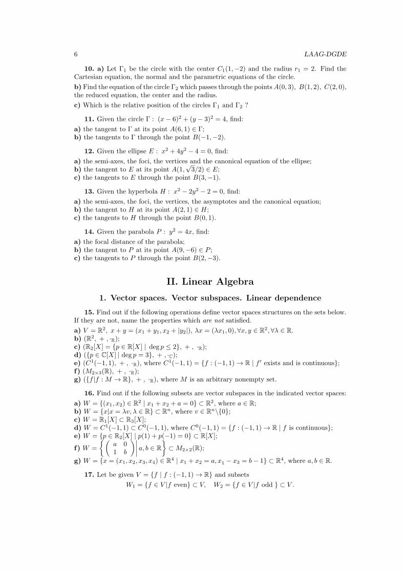
10. a) Let Γ1 be the circle with the center C1(1,−2) and the radius r1 = 2. Find theCartesian equation, the normal and the parametric equations of the circle.
b) Find the equation of the circle Γ2 which passes through the pointsA(0, 3), B(1, 2), C(2, 0),the reduced equation, the center and the radius.
c) Which is the relative position of the circles Γ1 and Γ2 ?
11. Given the circle Γ : (x− 6)2 + (y − 3)2 = 4, find:
a) the tangent to Γ at its point A(6, 1) ∈ Γ;b) the tangents to Γ through the point B(−1,−2).
12. Given the ellipse E : x2 + 4y2 − 4 = 0, find:
a) the semi-axes, the foci, the vertices and the canonical equation of the ellipse;b) the tangent to E at its point A(1,
√3/2) ∈ E;
c) the tangents to E through the point B(3,−1).
13. Given the hyperbola H : x2 − 2y2 − 2 = 0, find:
a) the semi-axes, the foci, the vertices, the asymptotes and the canonical equation;b) the tangent to H at its point A(2, 1) ∈ H;c) the tangents to H through the point B(0, 1).
14. Given the parabola P : y2 = 4x, find:
a) the focal distance of the parabola;b) the tangent to P at its point A(9,−6) ∈ P ;c) the tangents to P through the point B(2,−3).
II. Linear Algebra
1. Vector spaces. Vector subspaces. Linear dependence
15. Find out if the following operations define vector spaces structures on the sets below.If they are not, name the properties which are not satisfied.
a) V = R2, x+ y = (x1 + y1, x2 + |y2|), λx = (λx1, 0), ∀x, y ∈ R2,∀λ ∈ R.b) (R2, + , ·R);c) (R2[X] = {p ∈ R[X] | deg p ≤ 2}, + , ·R);d) ({p ∈ C[X] | deg p = 3}, + , ·C);e) (C1(−1, 1), + , ·R), where C1(−1, 1) = {f : (−1, 1) → R | f ′ exists and is continuous};f) (M2×3(R), + , ·R);g) ({f |f :M → R}, + , ·R), where M is an arbitrary nonempty set.
16. Find out if the following subsets are vector subspaces in the indicated vector spaces:
a) W = {(x1, x2) ∈ R2 | x1 + x2 + a = 0} ⊂ R2, where a ∈ R;b) W = {x|x = λv, λ ∈ R} ⊂ Rn, where v ∈ Rn\{0};c) W = R1[X] ⊂ R3[X];d) W = C1(−1, 1) ⊂ C0(−1, 1), where C0(−1, 1) = {f : (−1, 1) → R | f is continuous};e) W = {p ∈ R2[X] | p(1) + p(−1) = 0} ⊂ R[X];
f) W =
{(a 01 b
)∣∣∣∣ a, b ∈ R}
⊂M2×2(R);
g) W = {x = (x1, x2, x3, x4) ∈ R4 | x1 + x2 = a, x1 − x3 = b− 1} ⊂ R4, where a, b ∈ R.
17. Let be given V = {f | f : (−1, 1) → R} and subsets
W1 = {f ∈ V |f even} ⊂ V, W2 = {f ∈ V |f odd } ⊂ V .
Statements 7
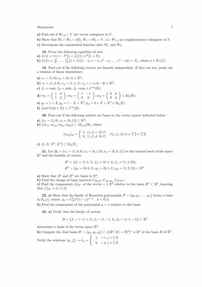
a) Find out if W1,2 ⊂ V are vector subspaces in V .
b) Show that W1 ∩W2 = {0}, W1 +W2 = V , i.e. W1,2 are supplementary subspaces in V .
c) Decompose the exponential function after W1 and W2.
18. Prove the following equalities of sets:a) L({1 + t, t, 1− t2}) = L({1, t, t2}) = P2;
b) L({1, x, x2
2! , . . . ,xn
n! }) = L({1− a, x− a, x2 − a, . . . , xn − a}) = Pn, where a ∈ R\{1}.
19. Find out if the following vectors are linearly independent. If they are not, point outa relation of linear dependence.
a) e1 = (1, 0), e2 = (0, 1) ∈ R2;
b) v1 = (1, 2, 0), v2 = (1, 1, 1), v3 = (−1, 0,−2) ∈ R3;
c) f1 = cosh, f2 = sinh, f3 =exp ∈ C∞(R);
d) m1 =
(1 01 2
);m2 =
(1 −10 0
);m3 =
(0 00 0
)∈M2(R);
e) p1 = 1 +X, p2 = 1−X +X2, p3 = 3 +X +X2 ∈ R2[X];
f) {cosk(t)|k ∈ N} ⊂ C∞(R).
20. Find out if the following subsets are bases in the vector spaces indicated below:
a) {e1 = (1, 0), e2 = (0, 1)} ⊂ R2;b) {m11,m12,m21,m22} ⊂M2×2(R), where
(mij)kl =
{1, (i, j) = (k, l)0, (i, j) = (k, l)
, ∀(i, j), (k, l) ∈ 1, 2× 1, 2;
c) {1, X,X2, X3} ⊂ R3[X].
21. Let B0 = {e1 = (1, 0, 0), e2 = (0, 1, 0), e3 = (0, 0, 1)} be the natural basis of the spaceR3 and the families of vectors:
B′ = {f1 = (1, 1, 1), f2 = (0, 1, 1), f3 = (1, 1, 0)};
B′′ = {g1 = (0, 0, 1), g2 = (0, 1, 1), g3 = (1, 2, 3)} ⊂ R3.
a) Show that B′ and B′′ are bases in R3;b) Find the change of basis matrices CB0B′ , CB′′B0
, CB′B′′ ;c) Find the components [v]B′′ of the vector v ∈ R3 relative to the basis B′′ ⊂ R3, knowingthat [v]B′ = (1, 1, 5).
22. a) Show that the family of Bernstein polynomials F = {p0, p1, . . . , pn} forms a basisin Rn[x], where pk = Cknx
k(1− x)n−k, k = 0, n.
b) Find the components of the polynomial q = 1 relative to this basis.
23. a) Verify that the family of vectors
B = {f1 = (−1, 1, 1), f2 = (1,−1, 1), f3 = (1, 1,−1)} ⊂ R3
determines a basis of the vector space R3.
b) Compute the dual basis B′ = {g1, g2, g3} ⊂ L(R3,R) = (R3)∗ ≡ R3 of the basis B of R3.
Verify the relations ⟨gi, fj⟩ = δij =
{1, i = j ∈ 1, 3
0, i = j ∈ 1, 3.
8 LAAG-DGDE
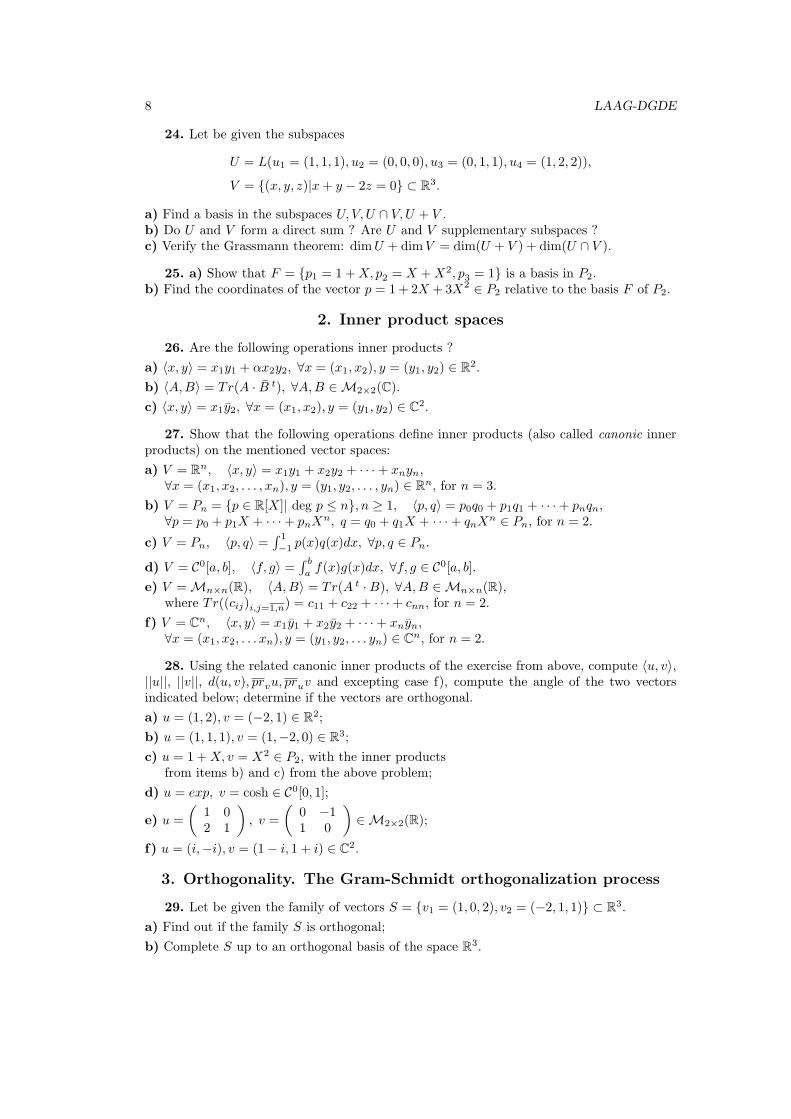
24. Let be given the subspaces
U = L(u1 = (1, 1, 1), u2 = (0, 0, 0), u3 = (0, 1, 1), u4 = (1, 2, 2)),
V = {(x, y, z)|x+ y − 2z = 0} ⊂ R3.
a) Find a basis in the subspaces U, V, U ∩ V,U + V .b) Do U and V form a direct sum ? Are U and V supplementary subspaces ?c) Verify the Grassmann theorem: dimU + dimV = dim(U + V ) + dim(U ∩ V ).
25. a) Show that F = {p1 = 1 +X, p2 = X +X2, p3 = 1} is a basis in P2.b) Find the coordinates of the vector p = 1+ 2X + 3X2 ∈ P2 relative to the basis F of P2.
2. Inner product spaces
26. Are the following operations inner products ?
a) ⟨x, y⟩ = x1y1 + αx2y2, ∀x = (x1, x2), y = (y1, y2) ∈ R2.
b) ⟨A,B⟩ = Tr(A · B t), ∀A,B ∈ M2×2(C).c) ⟨x, y⟩ = x1y2, ∀x = (x1, x2), y = (y1, y2) ∈ C2.
27. Show that the following operations define inner products (also called canonic innerproducts) on the mentioned vector spaces:
a) V = Rn, ⟨x, y⟩ = x1y1 + x2y2 + · · ·+ xnyn,∀x = (x1, x2, . . . , xn), y = (y1, y2, . . . , yn) ∈ Rn, for n = 3.
b) V = Pn = {p ∈ R[X]| deg p ≤ n}, n ≥ 1, ⟨p, q⟩ = p0q0 + p1q1 + · · ·+ pnqn,∀p = p0 + p1X + · · ·+ pnX
n, q = q0 + q1X + · · ·+ qnXn ∈ Pn, for n = 2.
c) V = Pn, ⟨p, q⟩ =∫ 1
−1p(x)q(x)dx, ∀p, q ∈ Pn.
d) V = C0[a, b], ⟨f, g⟩ =∫ baf(x)g(x)dx, ∀f, g ∈ C0[a, b].
e) V = Mn×n(R), ⟨A,B⟩ = Tr(A t ·B), ∀A,B ∈ Mn×n(R),where Tr((cij)i,j=1,n) = c11 + c22 + · · ·+ cnn, for n = 2.
f) V = Cn, ⟨x, y⟩ = x1y1 + x2y2 + · · ·+ xnyn,∀x = (x1, x2, . . . xn), y = (y1, y2, . . . yn) ∈ Cn, for n = 2.
28. Using the related canonic inner products of the exercise from above, compute ⟨u, v⟩,||u||, ||v||, d(u, v), prvu, pruv and excepting case f), compute the angle of the two vectorsindicated below; determine if the vectors are orthogonal.
a) u = (1, 2), v = (−2, 1) ∈ R2;
b) u = (1, 1, 1), v = (1,−2, 0) ∈ R3;
c) u = 1 +X, v = X2 ∈ P2, with the inner productsfrom items b) and c) from the above problem;
d) u = exp, v = cosh ∈ C0[0, 1];
e) u =
(1 02 1
), v =
(0 −11 0
)∈ M2×2(R);
f) u = (i,−i), v = (1− i, 1 + i) ∈ C2.
3. Orthogonality. The Gram-Schmidt orthogonalization process
29. Let be given the family of vectors S = {v1 = (1, 0, 2), v2 = (−2, 1, 1)} ⊂ R3.
a) Find out if the family S is orthogonal;
b) Complete S up to an orthogonal basis of the space R3.
Statements 9
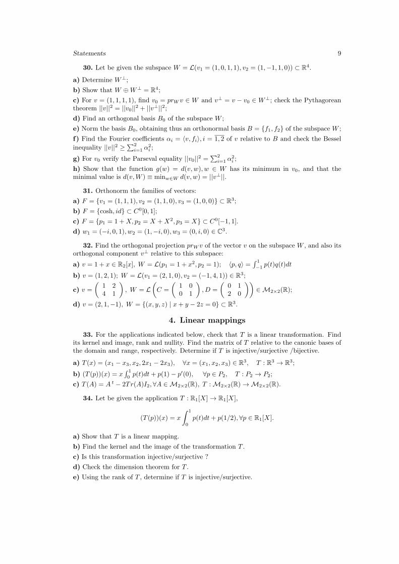
30. Let be given the subspace W = L(v1 = (1, 0, 1, 1), v2 = (1,−1, 1, 0)) ⊂ R4.
a) Determine W⊥;
b) Show that W ⊕W⊥ = R4;
c) For v = (1, 1, 1, 1), find v0 = prW v ∈ W and v⊥ = v − v0 ∈ W⊥; check the Pythagoreantheorem ||v||2 = ||v0||2 + ||v⊥||2;d) Find an orthogonal basis B0 of the subspace W ;
e) Norm the basis B0, obtaining thus an orthonormal basis B = {f1, f2} of the subspace W ;
f) Find the Fourier coefficients αi = ⟨v, fi⟩, i = 1, 2 of v relative to B and check the Bessel
inequality ||v||2 ≥∑2i=1 α
2i ;
g) For v0 verify the Parseval equality ||v0||2 =∑2i=1 α
2i ;
h) Show that the function g(w) = d(v, w), w ∈ W has its minimum in v0, and that theminimal value is d(v,W ) ≡ minw∈W d(v, w) = ||v⊥||.
31. Orthonorm the families of vectors:
a) F = {v1 = (1, 1, 1), v2 = (1, 1, 0), v3 = (1, 0, 0)} ⊂ R3;
b) F = {cosh, id} ⊂ C0[0, 1];
c) F = {p1 = 1 +X, p2 = X +X2, p3 = X} ⊂ C0[−1, 1].
d) w1 = (−i, 0, 1), w2 = (1,−i, 0), w3 = (0, i, 0) ∈ C3.
32. Find the orthogonal projection prW v of the vector v on the subspace W , and also itsorthogonal component v⊥ relative to this subspace:
a) v = 1 + x ∈ R2[x], W = L(p1 = 1 + x2, p2 = 1); ⟨p, q⟩ =∫ 1
−1p(t)q(t)dt
b) v = (1, 2, 1); W = L(v1 = (2, 1, 0), v2 = (−1, 4, 1)) ∈ R3;
c) v =
(1 24 1
), W = L
(C =
(1 00 1
), D =
(0 12 0
))∈ M2×2(R);
d) v = (2, 1,−1), W = {(x, y, z) | x+ y − 2z = 0} ⊂ R3.
4. Linear mappings
33. For the applications indicated below, check that T is a linear transformation. Findits kernel and image, rank and nullity. Find the matrix of T relative to the canonic bases ofthe domain and range, respectively. Determine if T is injective/surjective /bijective.
a) T (x) = (x1 − x3, x2, 2x1 − 2x3), ∀x = (x1, x2, x3) ∈ R3, T : R3 → R3;
b) (T (p))(x) = x∫ 1
0p(t)dt+ p(1)− p′(0), ∀p ∈ P2, T : P2 → P2;
c) T (A) = A t − 2Tr(A)I2, ∀A ∈ M2×2(R), T : M2×2(R) → M2×2(R).
34. Let be given the application T : R1[X] → R1[X],
(T (p))(x) = x
∫ 1
0
p(t)dt+ p(1/2), ∀p ∈ R1[X].
a) Show that T is a linear mapping.
b) Find the kernel and the image of the transformation T .
c) Is this transformation injective/surjective ?
d) Check the dimension theorem for T .
e) Using the rank of T , determine if T is injective/surjective.
10 LAAG-DGDE
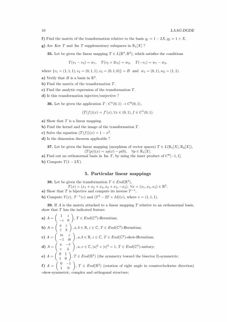
f) Find the matrix of the transformation relative to the basis q1 = 1− 2X, q2 = 1 +X.
g) Are Ker T and Im T supplementary subspaces in R1[X] ?
35. Let be given the linear mapping T ∈ L(R3,R2), which satisfies the conditions
T (v1 − v3) = w1, T (v2 + 2v3) = w2, T (−v1) = w1 − w2,
where {v1 = (1, 1, 1), v2 = (0, 1, 1), v3 = (0, 1, 0)} = B and w1 = (0, 1), w2 = (1, 1).
a) Verify that B is a basis in R3.
b) Find the matrix of the transformation T .
c) Find the analytic expression of the transformation T .
d) Is this transformation injective/surjective ?
36. Let be given the application T : C1(0, 1) → C0(0, 1),
(T (f))(x) = f ′(x), ∀x ∈ (0, 1), f ∈ C1(0, 1).
a) Show that T is a linear mapping.
b) Find the kernel and the image of the transformation T .
c) Solve the equation (T (f))(x) = 1− x2.
d) Is the dimension theorem applicable ?
37. Let be given the linear mapping (morphism of vector spaces) T ∈ L(R1[X],R2[X]),(T (p))(x) = xp(x)− p(0), ∀p ∈ R1[X].
a) Find out an orthonormal basis in Im T , by using the inner product of C0[−1, 1].
b) Compute T (1− 2X).
5. Particular linear mappings
38. Let be given the transformation T ∈ End(R3),T (x) = (x1 + x2 + x3, x2 + x3,−x3), ∀x = (x1, x2, x3) ∈ R3.
a) Show that T is bijective and compute its inverse T−1;
b) Compute T (v), T−1(v) and (T 3 − 2T + Id)(v), where v = (1, 1, 1).
39. If A is the matrix attached to a linear mapping T relative to an orthonormal basis,show that T has the indicated feature.
a) A =
(1 i−i 0
), T ∈ End(C2)-Hermitian;
b) A =
(a zz b
), a, b ∈ R, z ∈ C, T ∈ End(C2)-Hermitian;
c) A =
(ia z−z ib
), a, b ∈ R, z ∈ C, T ∈ End(C2)-skew-Hermitian;
d) A =
(u −vv u
), u, v ∈ C, |u|2 + |v|2 = 1, T ∈ End(C2)-unitary;
e) A =
(0 11 0
), T ∈ End(R2) (the symmetry toward the bisector I)-symmetric;
f) A =
(0 −11 0
), T ∈ End(R2) (rotation of right angle in counterclockwise direction)
-skew-symmetric, complex and orthogonal structure;
Statements 11
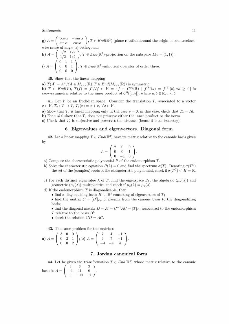
g) A =
(cosα − sinαsinα cosα
), T ∈ End(R2) (plane rotation around the origin in counterclock-
wise sense of angle α)-orthogonal;
h) A =
(1/2 1/21/2 1/2
), T ∈ End(R2)-projection on the subspace L(v = (1, 1));
i) A =
0 1 10 0 10 0 0
, T ∈ End(R3)-nilpotent operator of order three.
40. Show that the linear mapping
a) T (A) = A t,∀A ∈M2×2(R), T ∈ End(M2×2(R)) is symmetric;b) T ∈ End(V ), T (f) = f ′, ∀f ∈ V = {f ∈ C∞(R) | f (k)(a) = f (k)(b),∀k ≥ 0} isskew-symmetric relative to the inner product of C0([a, b]), where a, b ∈ R, a < b.
41. Let V be an Euclidian space. Consider the translation Tv associated to a vectorv ∈ V , Tv : V → V, Tv(x) = x+ v, ∀x ∈ V .
a) Show that Tv is linear mapping only in the case v = 0; in this case, check that Tv = Id.b) For v = 0 show that Tv does not preserve either the inner product or the norm.c) Check that Tv is surjective and preserves the distance (hence it is an isometry).
6. Eigenvalues and eigenvectors. Diagonal form
42. Let a linear mapping T ∈ End(R3) have its matrix relative to the canonic basis givenby
A =
2 0 00 0 10 −1 0
.
a) Compute the characteristic polynomial P of the endomorphism T .
b) Solve the characteristic equation P (λ) = 0 and find the spectrum σ(T ). Denoting σ(TC)the set of the (complex) roots of the characteristic polynomial, check if σ(TC) ⊂ K = R.
c) For each distinct eigenvalue λ of T , find the eigenspace Sλ, the algebraic (µa(λ)) andgeometric (µg(λ)) multiplicities and check if µa(λ) = µg(λ).
d) If the endomorphism T is diagonalizable, then:• find a diagonalizing basis B′ ⊂ R3 consisting of eigenvectors of T ;• find the matrix C = [B′]B0 of passing from the canonic basis to the diagonalizingbasis;• find the diagonal matrix D = A′ = C−1AC = [T ]B′ associated to the endomorphismT relative to the basis B′;• check the relation CD = AC.
43. The same problem for the matrices
a) A =
3 0 00 2 10 0 2
; b) A =
7 4 −14 7 −1−4 −4 4
.
7. Jordan canonical form
44. Let be given the transformation T ∈ End(R3) whose matrix relative to the canonic
basis is A =
3 3 3−1 11 62 −14 −7
.
12 LAAG-DGDE
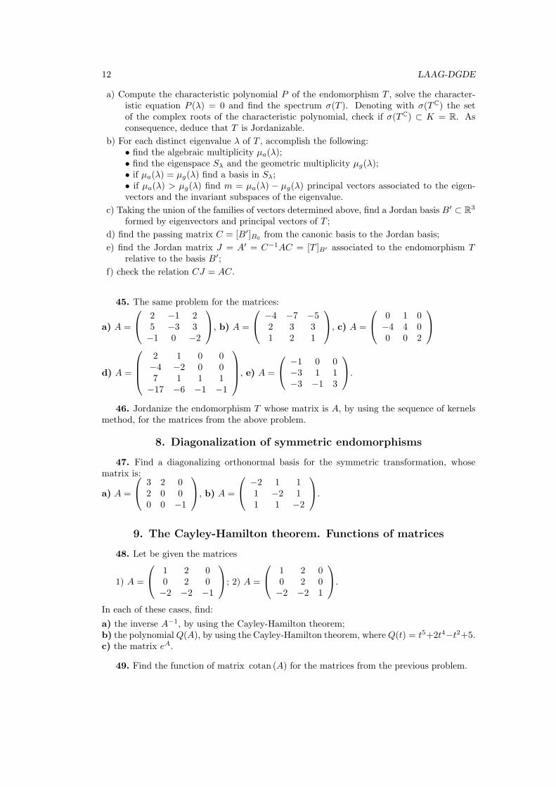
a) Compute the characteristic polynomial P of the endomorphism T , solve the character-istic equation P (λ) = 0 and find the spectrum σ(T ). Denoting with σ(TC) the setof the complex roots of the characteristic polynomial, check if σ(TC) ⊂ K = R. Asconsequence, deduce that T is Jordanizable.
b) For each distinct eigenvalue λ of T , accomplish the following:• find the algebraic multiplicity µa(λ);• find the eigenspace Sλ and the geometric multiplicity µg(λ);• if µa(λ) = µg(λ) find a basis in Sλ;• if µa(λ) > µg(λ) find m = µa(λ) − µg(λ) principal vectors associated to the eigen-vectors and the invariant subspaces of the eigenvalue.
c) Taking the union of the families of vectors determined above, find a Jordan basis B′ ⊂ R3
formed by eigenvectors and principal vectors of T ;
d) find the passing matrix C = [B′]B0 from the canonic basis to the Jordan basis;
e) find the Jordan matrix J = A′ = C−1AC = [T ]B′ associated to the endomorphism Trelative to the basis B′;
f) check the relation CJ = AC.
45. The same problem for the matrices:
a) A =
2 −1 25 −3 3−1 0 −2
, b) A =
−4 −7 −52 3 31 2 1
, c) A =
0 1 0−4 4 00 0 2
d) A =
2 1 0 0−4 −2 0 07 1 1 1
−17 −6 −1 −1
, e) A =
−1 0 0−3 1 1−3 −1 3
.
46. Jordanize the endomorphism T whose matrix is A, by using the sequence of kernelsmethod, for the matrices from the above problem.
8. Diagonalization of symmetric endomorphisms
47. Find a diagonalizing orthonormal basis for the symmetric transformation, whosematrix is:
a) A =
3 2 02 0 00 0 −1
, b) A =
−2 1 11 −2 11 1 −2
.
9. The Cayley-Hamilton theorem. Functions of matrices
48. Let be given the matrices
1) A =
1 2 00 2 0−2 −2 −1
; 2) A =
1 2 00 2 0−2 −2 1
.
In each of these cases, find:
a) the inverse A−1, by using the Cayley-Hamilton theorem;b) the polynomialQ(A), by using the Cayley-Hamilton theorem, whereQ(t) = t5+2t4−t2+5.c) the matrix eA.
49. Find the function of matrix cotan (A) for the matrices from the previous problem.
Statements 13
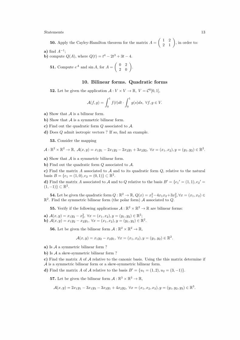
50. Apply the Cayley-Hamilton theorem for the matrix A =
(1 22 1
), in order to:
a) find A−1;b) compute Q(A), where Q(t) = t4 − 2t3 + 3t− 4.
51. Compute eA and sinA, for A =
(0 22 0
).
10. Bilinear forms. Quadratic forms
52. Let be given the application A : V × V → R, V = C0[0, 1],
A(f, g) =
∫ 1
0
f(t)dt ·∫ 1
0
g(s)ds, ∀f, g ∈ V.
a) Show that A is a bilinear form.
b) Show that A is a symmetric bilinear form.
c) Find out the quadratic form Q associated to A.
d) Does Q admit isotropic vectors ? If so, find an example.
53. Consider the mapping
A : R2 ×R2 → R, A(x, y) = x1y1 − 2x1y2 − 2x2y1 + 3x2y2, ∀x = (x1, x2), y = (y1, y2) ∈ R2.
a) Show that A is a symmetric bilinear form.
b) Find out the quadratic form Q associated to A.
c) Find the matrix A associated to A and to its quadratic form Q, relative to the naturalbasis B = {e1 = (1, 0), e2 = (0, 1)} ⊂ R2.
d) Find the matrix A associated to A and to Q relative to the basis B′ = {e1′ = (1, 1), e2′ =
(1,−1)} ⊂ R2.
54. Let be given the quadratic form Q : R2 → R, Q(x) = x21−4x1x2+3x22, ∀x = (x1, x2) ∈R2. Find the symmetric bilinear form (the polar form) A associated to Q.
55. Verify if the following applications A : R2 × R2 → R are bilinear forms:
a) A(x, y) = x1y2 − x22, ∀x = (x1, x2), y = (y1, y2) ∈ R2;b) A(x, y) = x1y2 − x2y1, ∀x = (x1, x2), y = (y1, y2) ∈ R2.
56. Let be given the bilinear form A : R2 × R2 → R,
A(x, y) = x1y2 − x2y1, ∀x = (x1, x2), y = (y1, y2) ∈ R2.
a) Is A a symmetric bilinear form ?
b) Is A a skew-symmetric bilinear form ?
c) Find the matrix A of A relative to the canonic basis. Using the this matrix determine ifA is a symmetric bilinear form or a skew-symmetric bilinear form.
d) Find the matrix A of A relative to the basis B′ = {u1 = (1, 2), u2 = (3,−1)}.
57. Let be given the bilinear form A : R3 × R3 → R,
A(x, y) = 2x1y1 − 3x1y3 − 3x3y1 + 4x2y2, ∀x = (x1, x2, x3), y = (y1, y2, y3) ∈ R3.
14 LAAG-DGDE
a) Show that A is a symmetric bilinear form.
b) Find the matrix of A relative to the canonic basis; check the result by using the relationA(x, y) = X tAY , where X and Y are the column vectors associated to x and y, respectively.
c) Find Ker A, rank A and check the dimension theorem: dim KerA+ rankA = dimR3.d) Find the quadratic form Q associated to A.
e) Is Q (and hence, the bilinear symmetric form A) degenerate or non-degenerate ? Does Qadmit non-zero isotropic vectors ?
58. Let be given the application A : V × V → R,
A(p, q) =
∫ 1
0
p(t)dt
∫ 1
0
q(s)ds, ∀p, q ∈ V = R2[X]
and B′ = {q1 = 1 +X, q2 = X2, q3 = 1} ⊂ V a basis of V . Answer to the questions a)-e) ofthe preceding problem.
59. Let be given the quadratic form Q : R3 → R,
Q(x) = x21 − x1x2 + 2x2x3, ∀x = (x1, x2, x3) ∈ R3.
a) Find the symmetric bilinear form A associated to Q (the polar form).b) Find the matrix of Q (of A) relative to the canonic basis.
60. Let be given the symmetric bilinear form A : R3 × R3 → R,
A(x, y) = 2x1y1 − 3x1y3 − 3x3y1 + 4x2y2, ∀x = (x1, x2, x3), y = (y1, y2, y3) ∈ R3.
a) Find U⊥, where U = L(v1 = (1, 1, 0), v2 = (0, 1, 1)).b) Does the equality U ⊕ U⊥ = R3 hold true?c) Is A (and hence Q) non-degenerate?
11. The canonical expression of a quadratic form
61. Let be given the quadratic form Q of matrix A =
0 1 −21 0 3−2 3 0
. Using the Gauss
method, find the canonical expression of Q and the corresponding basis B′.
62. Let be given the quadratic form Q : R2 → R, Q(x) = x21−4x1x2+x22, ∀x = (x1, x2) ∈
R2. Using the Jacobi method find the canonical expression of Q and the corresponding basisB′.
63. For the quadratic form the problem above, by using the method of eigenvalues, findthe canonical expression of Q and the corresponding basis B′. Show that the signature ofthe quadratic form Q is conserved.
64. Apply three methods (Gauss, eigenvalues and Jacobi) where is possible, in order toget the canonical expression and the signature for the following quadratic form Q given byits matrix A = [Q] (relative to the canonical basis) or through its analytical expression:
a) Q(v) = x2 − 8xy − 16xz + 7y2 − 8yz + z2, ∀v = (x, y, z) ∈ R3;
b) Q(x) = 4x1x2 − 5x22, ∀x = (x1, x2) ∈ R2;
c) A =
3 −2 −4−2 6 −2−4 −2 3
; d) A =
1 1 −11 2 0−1 0 3
;
Statements 15
e) Q(x) = −x21 + 6x1x3 + x22 + 4x2x3 − 5x23, ∀x = (x1, x2, x3) ∈ R3;
f) A =
0 1 −3 01 0 0 −3−3 0 0 10 −3 1 0
; g) A =
5 −2 −2−2 6 0−2 0 4
.
Are these quadratic forms positive/negative definite/semidefinite ? Are they degenerate/non-degenerate ?
III. Analytic Geometry
1. Free vectors
65. Let be given the free vectors a = i+ 2j + µk, b = i+ j + 2k ∈ V3, where µ ∈ R.a) Find the cross product a× b.
b) Is S = {a, b} a linearly independent family of vectors ? Are the two vectors non-collinear? If they are, complete S up to a basis of the space V3.
c) For µ = 2 find the areas of the triangle and of the parallelogram, which are determined bya and b as adjacent edges.
66. Let be given the vectors a = i+ j + k, b = µk + j, c = k + j ∈ V3, where µ ∈ R.a) Compute the joint (mixed) product ⟨a, b× c⟩.b) Are the three vectors linearly independent ? Are they non-coplanar ? If they are linearlyindependent, do they determine a positive oriented basis in V3 ?
c) For µ = 0 find the volumes of the tetrahedron, of the triangular prism and of the paral-lelepiped which are determined by a, b and c as adjacent edges.
67. Compute the volume of the tetrahedron determined by the points A(0, 0, 0), B(1, 0, 0),C(0, 1, 0), D(0, 0, 1).
68. Let be given the vectors a = i− j + k, b = i+ 2j + 3k, c = k + j.
a) Find double cross product w = a× (b× c).
b) Recalculate w by using the abbreviated formula w = ⟨a, c⟩b− ⟨a, b⟩c =∣∣∣∣ b c⟨a, b⟩ ⟨a, c⟩
∣∣∣∣.c) Show that w is perpendicular on a and coplanar with b and c.
2. The straight line and the plane in space
69. Find the straight line ∆ in each of the following cases:
a) ∆ ⊃ {A(1, 2, 3), B(4, 2, 1)};b) ∆ ∋ C(2, 6, 1) and ∆ admits the director vector v = 2k − i.
70. Find the parametric equations, two distinct points and a direction vector of the
straight line ∆ :
{2x+ y − 5z = 124x+ 7y − 33z = 1.
71. Find the plane π in each of these cases:
a) π ⊃ {A(1,−2, 1), B(2,−5, 1), C(3,−3, 1)}. Previously verify that A,B,C are not collinear.b) π ∋ D(1, 5, 0) and π has the normal direction given by n = 3j + 2k;
c) π ∋ E(2, 1, 2) and π is parallel with the directions u = 2i, v = 3k − i;
16 LAAG-DGDE
d) Determine the equation of the plane π, which is located at the distance d = 2 from theorigin-measured along the direction and sense of the normal vector n0 = i+ 2j − 2k.
72. Find the parametric equations, three non-collinear points and a normal vector of theplane x+ 2y − 3z = 4.
73. Find the plane π in each of the following cases:
a) It determines π on the three axes Ox,Oy,Oz segments measuring 1,−3, 2;
b) π ⊃ ∆ : x = 1− y = z−10 , π ∋ F (1, 2, 3);
c) π||π∗ : x− 3z + 1 = 0, π ∋ G(2, 0,−1).
3. Problems related to straight line and plane
74. Let be given the planes π1 : x− 3y = 1, π2 : 2y + z = 2 and the straight lines
∆1 :
{x− y = 2x+ z = 3
, ∆2 : 2x−13 = y+1
0 = 1− z.
a) Are the straight lines ∆1 and ∆2 parallel ? Are they intersecting ? But perpendicular ?
b) Are the planes π1 and π2 parallel ? Are they intersecting ? But perpendicular ?
75. Let be given the planes π1 : x−3y = 1, π2 : 2y+ z = 2, π : y− z = 1 and the straightlines
∆1 :
{x− y = 2x+ z = 3
, ∆2 : 2x−13 = y+1
0 = 1− z, ∆ : x−1−1 = y
2 = z+15 .
Find the angles:
a) of the straight lines ∆1 and ∆2;
b) of the straight line ∆ and the plane π;
c) of the planes π1 and π2.
76. Let be given the points A(1, 2, 3), B(−1, 0, 1), the plane π : y−z = 1 and the straightline ∆ : x−1
−1 = y2 = z+1
5 . Find the distances:
a) between the points A and B;
b) between the point A and the straight line ∆;
c) between the point A and the plane π.
77. Let be given: the point A(1, 2, 3), the plane π : y − z = 1 and the straight line∆ : x−1
−1 = y2 = z+1
5 . Find the projections:
a) the projection of the point A onto the plane π;
b) the projection of the point A onto the straight line ∆;
c) the projection of the straight line ∆ onto the plane π (homework).
78. Let be given the points A(1, 2, 3), B(−1, 0, 1), the plane π : y−z = 1, and the straightline ∆ : x−1
−1 = y2 = z+1
5 . Find the following:
a) the symmetric of the point A with respect to the point B;
b) the symmetric of the point A with respect to the straight line ∆;
c) the symmetric of the point A with respect to the plane π;
d) the symmetric of the straight line ∆ with respect to the plane π.
Statements 17
79. Find the common perpendicular of the straight lines
∆1 :
{x− y = 2x+ z = 3
and ∆2 :2x− 1
3=y + 1
0= 1− z.
80. Show that the straight lines ∆1 :
{x− y = 2x+ z = 3
and ∆2 : 2x−13 = y+1
0 = 1 − z have
different directions, and find the distance between them.
81. Show that the straight lines ∆1 :
{x− y = 2x+ z = 3
and ∆2 : −2x−12 = 1− y = z− 1 have
the same direction, and find the distance between them.
4. Curvilinear coordinates
82. a) Find the polar coordinates (ρ, θ) for the point A whose Cartesian coordinates are(x, y) = (1,−2);
b) Find the Cartesian coordinates (x, y) for the point B whose polar coordinates are (ρ, θ) =(2, 3π4 ).
83. a) Find the cylindrical coordinates (ρ, θ, z) for the point C whose Cartesian coordi-nates are (x, y, z) = (1,−2,−3);
b) Find the Cartesian coordinates for the pointD whose cylindrical coordinates are (ρ, θ, z) =(1, 4π3 , 2).
84. a) Find the spherical coordinates for the point E whose Cartesian coordinates are(x, y, z) = (1,−2,−3);
b) Find the Cartesian coordinates for the point F whose spherical coordinates are (r, φ, θ) =(1, 2π3 ,
5π3 ).
5. Conics
85. Find the conic whose graph passes through the pointsA(1, 1), B(1,−1), C(−1, 1), D(−1,−1),E( 12 , 0), its type and nature.
86. Find the conics whose graph passes through the pointsA(0, 1), B(−1, 0), C(0,−1), D(1, 0).
87. Find the conics whose graph passes through the points A(1, 0), B(0, 0), C(0, 1).
88. Let be given the conic Γ : 4xy − 3y2 + 4x− 14y − 7 = 0.
a) Show that Γ is a hyperbola.
b) Find the center of the hyperbola Γ.
c) Find its axes, the asymptotes and its vertices.
d) Plot the hyperbola.
89. Let be given the conic Γ : 9x2 + 6xy + y2 − 4x− 8y − 4 = 0.
a) Show that Γ is a parabola.
b) Find the symmetry axis and the vertex of the conic.
c) Using the intersections with axes Ox and Oy, plot the conic.
90. Let be given the conic Γ : 16x2 + 4xy + 19y2 + 80x+ 10y + 40 = 0.
18 LAAG-DGDE
a) Show that Γ is an ellipse.
b) Find the center of the ellipse Γ.
c) Find the axes and the vertices of the ellipse.
d) Plot the conic.
91. Let be given the conic Γ : x2 − 2xy + 3y2 − 4x+ 6y − 4 = 0. Find:
a) the polar relative to A(1, 2) and the tangents from A to the conic.
b) the conjugate diameter with v = i− 2j and the tangents of direction v to the conic.
c) the tangent taken from the point B(1, 1) to the conic.
92. Let be given the conic Γ : 4xy − 3y2 + 4x− 14y − 7 = 0. Using the roto-translationmethod and the method of eigenvalues, find the canonic equation and plot.
93. Let be given the parabola Γ : 9x2 + 6xy + y2 − 4x − 8y − 4 = 0. Using the roto-translation method and the method of eigenvalues, find the canonical equation and plot.
94. Using the roto-translation method and the method of eigenvalues, find the canonicalequation and plot the conic 16x2 + 4xy + 19y2 + 80x+ 10y + 40 = 0.
6. Quadrics
95. Consider the sphere Σ : x2 + y2 + z2 + 2x− 6y + 4z + 10 = 0.
a) Find the center C and the radius r of the sphere.
b) Show that Σ intersects the plane π : 4x+ y + 3z + 13 = 0 after a circle.
c) Find the center C and the radius r of the intersection circle of the sphere with plane π.
96. Let be given the quadrics:
Σ1 : x2 − y2 + z2 − 2xy − 2yz − 2zx− 5x− 1 = 0;
Σ2 : −2√3xy + 2y2 − 7z2 + 112x− 16y − 14z − 87 = 0;
Σ3 : x2 + y2 + 5z2 − 6xy + 2xz − 2yz − 4x+ 8y − 12z + 14 = 0.
For each of the three quadrics:
a) compute the invariants ∆, δ, J, I;
b) find the symmetry center Cs of the quadric;
c) find the canonical equation of the quadric by using roto-translation method: get therotation matrix by using the method of eigenvalues;
d) plot the quadric.
97. Find the tangent plane π to the quadric x2
9 +y2 = 2z, which passes through the pointA(−3,−1, 1).
98. Find the angle formed by the rulers contained in the quadric x2
9 − z2
4 = y, which passthrough its point M(3, 1, 0); determine the tangent plane to the quadric and the normal lineto the quadric at its point M .
Statements 19
7. Generated surfaces
99. Find the cylindrical surface which has the director curve Γ :
{x = y2
z = 0and whose
generators are parallel with the straight line ∆′ : x−11 = y = 1−z
−1 .
100. Find the conical surface with the vertex V (1, 0, 0) and the director curve Γ :{x2 + y2 = 1x− z = 0.
101. Find the rotation surface generated through the rotation of the straight line ∆around the axis Oy:
a) ∆ : x−10 = y+2
2 = z−30 ;
b) ∆ : x3 = y+21 = z
−1 ;
c) ∆ : x3 = y+21 = z−3
−1 .
IV. Differential Geometry
1. Differentiable mappings
102. Let be given the function f : R → R2, f(s) = (s2, s3). Study if f is:
a) injective/surjective/bijective; in the last case, determine its inverse;
b) immersion/submersion/diffeomorphism; compute first the Jacobian matrix of the func-tion.
103. The same assertion for f : R → R3, f(t) = (2 cos2 t, sin 2t, 2 sin t), t ∈ (0, π2 ).
104. The same assertion for f : R2 → R2, f(u, v) = (u + v, uv), (u, v) ∈ R2. Computef−1({(0, 1)}) and Im (f).
105. Show that the following application is a diffeomorphism and compute its inverse:
f : (0,∞)× [0, 2π) → R2\{(0, 0)}, f(ρ, θ) = (ρ cos θ, ρ sin θ).
2. Curves in Rn
106. Find the normal hyperplane and the tangent straight line to the curveα : R → R4, α(t) = (t4,−1, t5, t6 + 2) at the point A(1,−1, 1, 3).
107. The same problem for the curve in problem 1 and at the point B(0,−1, 0, 2). Is αa regular curve ? Find the singularities of the curve, and the order of singularity.
108. Find the angle formed between the curves
α(t) = (t2 + 1, ln t, t), t > 0, β(s) = (2 + s, s, s+ 1), s ∈ R
at their common point.
109. Study the asymptotic behavior of the curve α(t) =(t− 1, t2
t−1
), α : R\{1} → R2.
110. Let be given the cycloid α(t) = (a(t− sin t), a(1− cos t)), t ∈ R, (a > 0).
a) Find the arc-length of the curve Γ = α([0, 2π]).
b) Find the normal parameter of the curve and its normal parameterization for t ∈ (0, 2π).
20 LAAG-DGDE
3. Planar curves
111. Let be given the curve α(t) = (t2, 3t), t ∈ R. Find the tangent, the normal, thesubtangent and the subnormal of the curve at its point A(1,−3).
112. Let be given the curve Γ : x2 − y3 − 3 = 0.
a) Find the tangent and the normal to the curve at its point A(−2, 1).
b) Parameterize the curve α.
113. Let be given the parabola α(t) = (t, t2), t ∈ R. Find:
a) the Frenet elements of the curve (the Frenet unit vectors and the curvature of the curve)and check the Frenet equation;
b) the Frenet elements of the curve at the point A(−2, 4);c) the equation of the osculating circle at the point A of the curve;
d) the evolute of the curve;
e) the Cartesian equation of the curve.
114. Compute the curvature of the parabola Γ : y = x2 at the point A(2, 4), using thecurvature formulas for:
a) parametric equations;b) explicit Cartesian equations;c) implicit Cartesian equations.
115. Find the envelope of the family of curves, in each of the following cases:
a) Γa : (x− a)2 + y2 − a2
2 = 0, a ∈ R;b) Γα : x · cosα+ y · sinα = 2, α ∈ [0, 2π];
c) Γλ : x2 + y2 − 2λx+ λ2 − 4λ = 0, λ ∈ R.
116. Let be given the curve Γ : x3 − 2y2 = 0.
a) find the tangent and the normal to the curve at the point A(2,−1) ∈ Γ;
b) find the singular points, their type, and the tangent and the normal at these points. Is Γa regular curve ?
117. Plot the graph of the curve α(t) = (2− t+ 1t , 2 + t+ 1
t ), t ∈ R∗.
118. Let be given the following curves:
a) Γ1 : y2(a− x)− x3 = 0 (cissoid of Diocles);
b) Γ2 : x3 + y3 − 3axy = 0 (folium of Descartes);
c) Γ3 : x(x2 + y2) + a(y2 − x2) = 0 (strophoide).
In each of the three cases, determine a parameterization of the curve by using the substitutiony = tx (where t is the parameter); find the polar equation; by using this equation, find theasymptotic direction and the asymptotic lines of the curve.
119. Let be given the curves:
a) Archimedes’ spiral Γ1 : ρ = aθ (a > 0);
b) the exponential spiral Γ2 : ρ = eθ, θ ∈ R.In each of the two cases determine the tangent and the normal equations relative to the polarmoving frame and compute the curvature.
Statements 21
4. Space curves
120. Let be given the curve α(t) = (2 cos t, 2 sin t, t), t ∈ R.
a) find the Frenet elements at an arbitrary point of the curve and check that the Frenetequations hold true;
b) find the Frenet elements at the point A(−2, 0, π);c) show that α is a helix;
d) find the Cartesian equations of the curve;
e) find the edges and the faces of the Frenet frame.
121. Let be given the curve α(t) = (t+ t2, t2 − t, t2 − t), t ∈ R. Show that α:
a) the osculating plane is independent of t (as a consequence, it contains the image of thecurve);
b) has the torsion identically equal to zero;
c) has the binormal vector field independent of t.
122. Let be given the curve Γ :
{x2 + y2 + z2 = 2z = 1.
a) find the tangent line and the normal plane to the curve at A(−1, 0, 1);
b) determine a parameterization of the curve.
5. Surfaces
123. Let be given the application r(u, v) = (u cos v, u sin v, u2), where (u, v) ∈ D =(0,∞)× [0, 2π).
a) Compute the partial velocities of the surface. Is r a map ?
b) Find the normal line and the tangent plane to Σ = r(D) ⊂ R3 at its point A(−2, 0, 4);
c) find the field n of unit vectors normal to the surface Σ ? Find the Gauss frame of thesurface ?
d) Find the Cartesian equation of the surface Σ. What does it represent ?
e) Characterize the coordinate curves of the surface ? Find their Cartesian equations;
f) find the angle formed by the coordinate curves at the point A.
124. Let be given the set of points Σ described by the equation x3 − z + 1 = 0
a) Is Σ a surface ?
b) Find the field n of unit vectors normal to the surface Σ.
c) Find the normal line and the tangent plane to Σ at A(1, 0, 2).
125. Find the envelope Σ of the family of planes
ax+ by +√
1− a2 − b2z − p = 0,
where p > 0 is fixed and a, b are real parameters which satisfy the condition a2 + b2 ≤ 0.
126. Using the parametric equations and the Cartesian equations of the following simplesurface, show that:
a) r(u, v) = (u cos v, u sin v, v), (u, v) ∈ R2 is a helicoid with director plane;
b) r(u, v) = (cosu, sinu, v), (u, v) ∈ (0, 2π)× R is a cylindrical surface;
22 LAAG-DGDE
c) r(u, v) = (v cosu, v sinu, v), (u, v) ∈ (0, 2π)× R is a conical surface.
127. Let be given the parametrized surface r(u, v) = (u cos v, u sin v, v), (u, v) ∈ R2.
a) Find the matrices of the three fundamental forms [I], [II], [III] of the surface.
b) Find the angle formed by the coordinate curves; is the Gauss frame orthonormal ?
c) Find the total curvature (the Gauss curvature) K and the mean curvature H of the surface.
d) Is the given surface unfolding ? But minimal ? What kind of points has the given surface(elliptic/parabolic/hyperbolic) ?
e) Test the Beltrami-Enneper formula [III]− 2H[II] +K[I] = [0].
128. For the parametrized surface r(u, v) = (u cos v, u sin v, v), (u, v) ∈ R2:
a) determine the matrix of the Weingarten operator;
b) find the principal curvatures k1 and k2 and the principal directions of the surface at anarbitrary point of this, by using the Weingarten operator matrix. Find the same curvaturesby using K and H;
c) determine the normal curvature of the surface in the tangent direction given by the vectorw = 2ru − rv in the point A(−1, 0, π) of the surface;
d) find the quadratic approximation of the surface in the point A.
129. a) Check the Meusnier formula for the helix α = r ◦ (u, v) on the cylinder Σ = Im r,where r(u, v) = (cosu, sinu, v), u(t) = v(t) = t, t ∈ R.b) Let α be the curve obtained through sectioning the circular cylinder Σ = Im r,
r(u, v) = (cosu, sinu, v), (u, v) ∈ D = [0, 2π)× R ⊂ R2,
with the plane z = x. Determine a parameterization of the curve α and verify the Meusnierformula.
130. Apply the Euler Theorem for the velocity vectors of the curves from the previousproblem.
131. For the parametrized surface r(u, v) = (u cos v, u sin v, v), (u, v) ∈ R2:
a) determine the length of the curve Γv=2u, u ∈ [1, 2].
b) find the area of the zone which corresponds to the domain (u, v) ∈ [0, 1]× [0, π].
132. For the cylinder r(u, v) = (cosu, sinu, v), (u, v) ∈ [0, 2π)× R, determine:
a) the curvature lines (the principal curves);
b) the asymptotic curves;
c) the geodesics.
V. Differential Equations
1. Ordinary differential equations
133. Show that the function y(x) given by the implicit relation sin y − cx = 0, (c ∈ R)satisfies the differential equation xy′ cos y − sin y = 0.
Statements 23
134. Find the general solution of the differential equation with separable variables xy′ cos y−sin y = 0.
135. Integrate the following homogeneous differential equations, showing that they arereducible to equations with separable variables:
a) x2y′ − y2 = 0;b) y′ · cos yx = sin y
x .
136. Integrate the following differential equations, showing that they are reducible toequations with separable variables.
a) (x+ y − 1)dx+ (x− y − 1)dy = 0;
b) (x+ y − 1)dx+ (x+ y)dy = 0.
137. Integrate the following linear differential equations:
a) xy′ + 2y = 3x, y(1) = 1
b) xy′ + 3y = x2.
138. Show that the following equations are Bernoulli equations and integrate
a) y′ = y − x√y;
b) dy = (xy − xy3)dx.
139. Integrate the following Riccati equations, knowing that they admit the particularsolution shown below
a) y′ = x · y2 − y, y1 = 1x+a , (a ∈ R);
b) y′ + y2 = 2x2 , y1 = a
x , (a ∈ R).
140. Integrate the following differential exact equations, previously checking that theequations are of such type:
a) (x+ y) + (x+ 2y) · y′ = 0;
b) (x2 + y2 + 2x)dx+ 2xydy = 0.
141. Show that the following equations admit integrating factor and then integrate:
a) (xy − x2)dy − y2dx = 0;
b) (5x2 + 12xy − 3y2)dx+ (3x2 − 2xy)dy = 0;
c) y′ · xy + 1 = 0.
142. Show that the following equation is of Clairaut type and then find its solution:y = xy′ − ln y′.
143. Show that the following equations are of Lagrange type and then integrate:
a) y = 2xy′ − y′2;
b) y − (y′)2 − 2(y′)3 = 0.
2. Higher order differential equations
144. Integrate the linear homogeneous differential equations of order 2 with constantcoefficients:
a) y′′ + 2y′ − 3y = 0;
24 LAAG-DGDE
b) y′′ + 4y = 0.
145. Solve the boundary problem (with constraints)
{y′′ + 2y′ − 3y = 0y(0) = −1, y(−1) = 0.
146. The same problem for x2y′′ − 3xy′′ + 4y = 0, y(e) = e2, y(1) = 0.
147. Integrate the following linear non-homogenous differential equations:
a) y′′ + 2y′ − 3y = e−3x;
b) y′′′ − y′′ − y′ + y = x · cosx;c) y′′ − y = x · ex;
d) the Cauchy problem:
{yIV − y = 8ex
y(0) = 0, y′′′(0) = 6, y′′(0) = 2, yIV (0) = 4.
148. (Isogonal trajectories). Let be given the family of lines Γm : y = mx, m ∈ R.
a) Find the differential equation of the family of these curves.
b) Find the orthogonal trajectories to the given family.
c) Find the curves (isogonal trajectories) which form with the given family an angle of 45o.
149. Show that the following equations admit a reduction of their order.
a) xy′′′ − y′′ = 0;
b) 2yy′ = y′2 + 1;
c) xy′ + y′′ = 0.
3. Systems of differential equations
150. Solve the system of homogeneous linear differential equations
{x′ = yy′ = x.
151. Use the result obtained at problem 1) in order to find the general solution of the
non-homogenous differential system
{x′ = yy′ = x+ 2.
152. Solve the Cauchy problem
{x′ = yy′ = x+ 2
,
{x(0) = 0y(0) = 2.
153. Solve the differential system
{x′ = yy′ = x+ 2
by using the elimination method.
154. Solve the higher-order linear differential equation with constant coefficientsy′′ − y = 2, where the unknown function is y = y(x).
155. Solve the Cauchy problem
{y′′ − y = 2y(0) = 1, y′(0) = 2.
4. Stability
156. Find if the solution X(t) = (x(t), y(t))t of the differential system X ′ = AX is stableor asymptotically stable, knowing that σ(A) = {−1,−2}.
157. The same problem, in the following cases:
a) σ(A) = {−2,±i}; b) σ(A) = {±2i}; c) σ(A) = {2,±i}.
Statements 25
5. Field lines (symmetric systems, prime integrals)
158. Find the field lines of the following vector fields by using the method of integrablecombinations:
a) X(x,y,z) = (x, y, x+ y);
b) X(x,y,z) = (x2, xy, y2).
159. Find the general solution for the following linear homogeneous differential equationswith partial derivatives:
a) x∂u
∂x+ y
∂u
∂y+ (x+ y)
∂u
∂z= 0;
b) x2∂u
∂x+ xy
∂u
∂y+ y2
∂u
∂z= 0.
160. Find that field surface Σ : u(x, y, z) = 0 of the field X, which contains the curve Γ.Consider the following cases:
a) X = (x, y, x+ y), Γ :
{y = 1z = x2
(a parabola).
b) X = (x2, xy, y2), Γ :
{y = 1z = x3
(a cubic curve).
Solutions
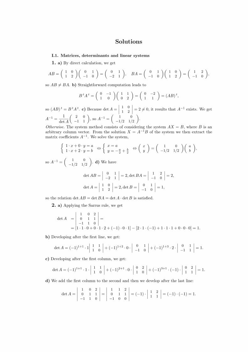
I.1. Matrices, determinants and linear systems
1. a) By direct calculation, we get
AB =
(1 01 2
)(0 1−1 0
)=
(0 1−2 1
), BA =
(0 1−1 0
)(1 01 2
)=
(1 2−1 0
),
so AB = BA. b) Straightforward computation leads to
B tA t =
(0 −11 0
)(1 10 2
)=
(0 −21 1
)= (AB) t,
so (AB) t = B tA t. c) Because detA =
∣∣∣∣ 1 01 2
∣∣∣∣ = 2 = 0, it results that A−1 exists. We get
A−1 =1
detA
(2 0−1 1
), so A−1 =
(1 0
−1/2 1/2
).
Otherwise. The system method consists of considering the system AX = B, where B is anarbitrary column vector. From the solution X = A−1B of the system we then extract thematrix coefficients A−1. We solve the system,{
1 · x+ 0 · y = a1 · x+ 2 · y = b
⇔{x = ay = −a
2 + b2
⇔(
xy
)=
(1 0
−1/2 1/2
)(ab
),
so A−1 =
(1 0
−1/2 1/2
). d) We have
detAB =
∣∣∣∣ 0 1−2 1
∣∣∣∣ = 2,detBA =
∣∣∣∣ 1 2−1 0
∣∣∣∣ = 2,
detA =
∣∣∣∣ 1 01 2
∣∣∣∣ = 2, detB =
∣∣∣∣ 0 1−1 0
∣∣∣∣ = 1,
so the relation detAB = detBA = detA · detB is satisfied.
2. a) Applying the Sarrus rule, we get
detA =
∣∣∣∣∣∣1 0 20 1 1−1 1 0
∣∣∣∣∣∣ == [1 · 1 · 0 + 0 · 1 · 2 + (−1) · 0 · 1]− [2 · 1 · (−1) + 1 · 1 · 1 + 0 · 0 · 0] = 1.
b) Developing after the first line, we get:
detA = (−1)1+1 · 1∣∣∣∣ 1 11 0
∣∣∣∣+ (−1)1+2 · 0 ·∣∣∣∣ 0 1−1 0
∣∣∣∣+ (−1)1+3 · 2 ·∣∣∣∣ 0 1−1 1
∣∣∣∣ = 1.
c) Developing after the first column, we get:
detA = (−1)1+1 · 1 ·∣∣∣∣ 1 11 0
∣∣∣∣+ (−1)2+1 · 0 ·∣∣∣∣ 0 21 0
∣∣∣∣+ (−1)3+1 · (−1) ·∣∣∣∣ 0 21 1
∣∣∣∣ = 1.
d) We add the first column to the second and then we develop after the last line:
detA =
∣∣∣∣∣∣1 0 20 1 1−1 1 0
∣∣∣∣∣∣ =∣∣∣∣∣∣
1 1 20 1 1−1 0 0
∣∣∣∣∣∣ = (−1) ·∣∣∣∣ 1 21 1
∣∣∣∣ = (−1) · (−1) = 1.
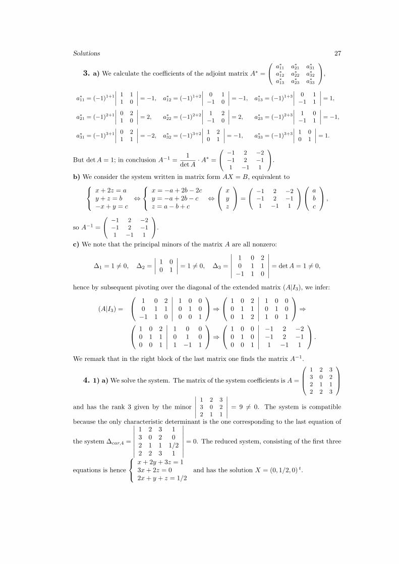
Solutions 27
3. a) We calculate the coefficients of the adjoint matrix A∗ =
a∗11 a∗
21 a∗31
a∗12 a∗
22 a∗32
a∗13 a∗
23 a∗33
,
a∗11 = (−1)1+1
∣∣∣∣ 1 11 0
∣∣∣∣ = −1, a∗12 = (−1)1+2
∣∣∣∣ 0 1−1 0
∣∣∣∣ = −1, a∗13 = (−1)1+3
∣∣∣∣ 0 1−1 1
∣∣∣∣ = 1,
a∗21 = (−1)2+1
∣∣∣∣ 0 21 0
∣∣∣∣ = 2, a∗22 = (−1)2+2
∣∣∣∣ 1 2−1 0
∣∣∣∣ = 2, a∗23 = (−1)2+3
∣∣∣∣ 1 0−1 1
∣∣∣∣ = −1,
a∗31 = (−1)3+1
∣∣∣∣ 0 21 1
∣∣∣∣ = −2, a∗32 = (−1)3+2
∣∣∣∣ 1 20 1
∣∣∣∣ = −1, a∗33 = (−1)3+3
∣∣∣∣ 1 00 1
∣∣∣∣ = 1.
But detA = 1; in conclusion A−1 =1
detA·A∗ =
−1 2 −2−1 2 −11 −1 1
.
b) We consider the system written in matrix form AX = B, equivalent to x+ 2z = ay + z = b−x+ y = c
⇔
x = −a+ 2b− 2cy = −a+ 2b− cz = a− b+ c
⇔
xyz
=
−1 2 −2−1 2 −11 −1 1
a
bc
,
so A−1 =
−1 2 −2−1 2 −11 −1 1
.
c) We note that the principal minors of the matrix A are all nonzero:
∆1 = 1 = 0, ∆2 =
∣∣∣∣ 1 00 1
∣∣∣∣ = 1 = 0, ∆3 =
∣∣∣∣∣∣1 0 20 1 1−1 1 0
∣∣∣∣∣∣ = detA = 1 = 0,
hence by subsequent pivoting over the diagonal of the extended matrix (A|I3), we infer:
(A|I3) =
1 0 20 1 1−1 1 0
∣∣∣∣∣∣1 0 00 1 00 0 1
⇒
1 0 20 1 10 1 2
∣∣∣∣∣∣1 0 00 1 01 0 1
⇒
1 0 20 1 10 0 1
∣∣∣∣∣∣1 0 00 1 01 −1 1
⇒
1 0 00 1 00 0 1
∣∣∣∣∣∣−1 2 −2−1 2 −11 −1 1
.
We remark that in the right block of the last matrix one finds the matrix A−1.
4. 1) a) We solve the system. The matrix of the system coefficients is A =
1 2 33 0 22 1 12 2 3
and has the rank 3 given by the minor
∣∣∣∣∣∣1 2 33 0 22 1 1
∣∣∣∣∣∣ = 9 = 0. The system is compatible
because the only characteristic determinant is the one corresponding to the last equation of
the system ∆car,4 =
∣∣∣∣∣∣∣∣1 2 3 13 0 2 02 1 1 1/22 2 3 1
∣∣∣∣∣∣∣∣ = 0. The reduced system, consisting of the first three
equations is hence
x+ 2y + 3z = 13x+ 2z = 02x+ y + z = 1/2
and has the solution X = (0, 1/2, 0) t.
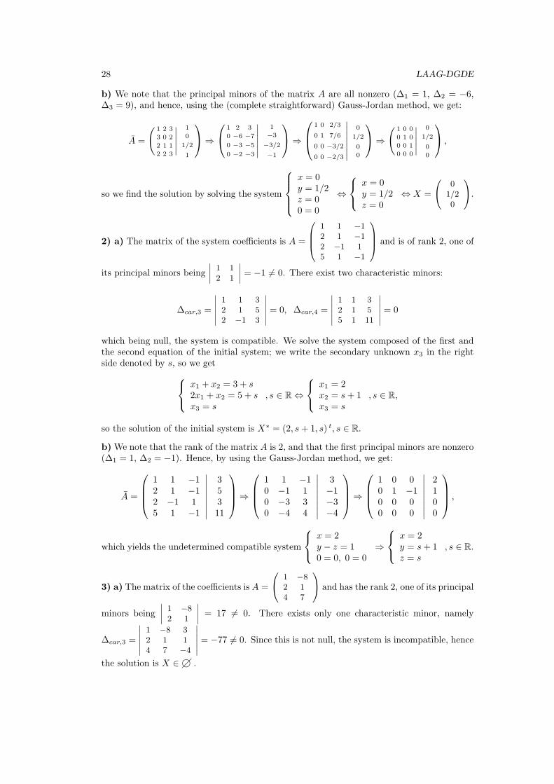
28 LAAG-DGDE
b) We note that the principal minors of the matrix A are all nonzero (∆1 = 1, ∆2 = −6,∆3 = 9), and hence, using the (complete straightforward) Gauss-Jordan method, we get:
A =
( 1 2 3
3 0 2
2 1 1
2 2 3
∣∣∣∣∣1
0
1/2
1
⇒
1 2 3
0 −6 −7
0 −3 −5
0 −2 −3
∣∣∣∣∣∣1
−3
−3/2
−1
⇒
1 0 2/3
0 1 7/6
0 0 −3/2
0 0 −2/3
∣∣∣∣∣∣∣0
1/2
0
0
⇒
( 1 0 0
0 1 0
0 0 1
0 0 0
∣∣∣∣∣0
1/2
0
0
,
so we find the solution by solving the system
x = 0y = 1/2z = 00 = 0
⇔
x = 0y = 1/2z = 0
⇔ X =
01/20
.
2) a) The matrix of the system coefficients is A =
1 1 −12 1 −12 −1 15 1 −1
and is of rank 2, one of
its principal minors being
∣∣∣∣ 1 12 1
∣∣∣∣ = −1 = 0. There exist two characteristic minors:
∆car,3 =
∣∣∣∣∣∣1 1 32 1 52 −1 3
∣∣∣∣∣∣ = 0, ∆car,4 =
∣∣∣∣∣∣1 1 32 1 55 1 11
∣∣∣∣∣∣ = 0
which being null, the system is compatible. We solve the system composed of the first andthe second equation of the initial system; we write the secondary unknown x3 in the rightside denoted by s, so we get x1 + x2 = 3 + s
2x1 + x2 = 5 + sx3 = s
, s ∈ R ⇔
x1 = 2x2 = s+ 1x3 = s
, s ∈ R,
so the solution of the initial system is X∗ = (2, s+ 1, s) t, s ∈ R.
b) We note that the rank of the matrix A is 2, and that the first principal minors are nonzero(∆1 = 1, ∆2 = −1). Hence, by using the Gauss-Jordan method, we get:
A =
1 1 −12 1 −12 −1 15 1 −1
∣∣∣∣∣∣∣∣35311
⇒
1 1 −10 −1 10 −3 30 −4 4
∣∣∣∣∣∣∣∣3−1−3−4
⇒
1 0 00 1 −10 0 00 0 0
∣∣∣∣∣∣∣∣2100
,
which yields the undetermined compatible system
x = 2y − z = 10 = 0, 0 = 0
⇒
x = 2y = s+ 1z = s
, s ∈ R.
3) a) The matrix of the coefficients is A =
1 −82 14 7
and has the rank 2, one of its principal
minors being
∣∣∣∣ 1 −82 1
∣∣∣∣ = 17 = 0. There exists only one characteristic minor, namely
∆car,3 =
∣∣∣∣∣∣1 −8 32 1 14 7 −4
∣∣∣∣∣∣ = −77 = 0. Since this is not null, the system is incompatible, hence
the solution is X ∈ g� .
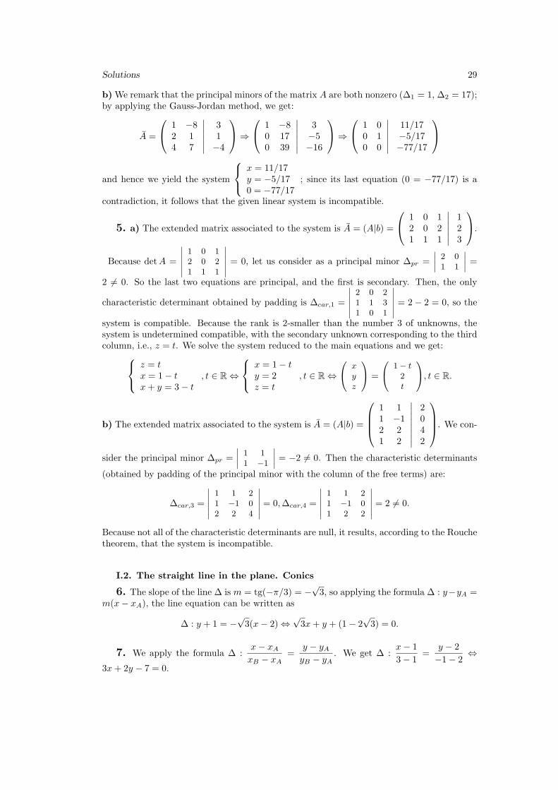
Solutions 29
b) We remark that the principal minors of the matrix A are both nonzero (∆1 = 1, ∆2 = 17);by applying the Gauss-Jordan method, we get:
A =
1 −82 14 7
∣∣∣∣∣∣31−4
⇒
1 −80 170 39
∣∣∣∣∣∣3−5−16
⇒
1 00 10 0
∣∣∣∣∣∣11/17−5/17−77/17
and hence we yield the system
x = 11/17y = −5/170 = −77/17
; since its last equation (0 = −77/17) is a
contradiction, it follows that the given linear system is incompatible.
5. a) The extended matrix associated to the system is A = (A|b) =
1 0 12 0 21 1 1
∣∣∣∣∣∣123
.
Because detA =
∣∣∣∣∣∣1 0 12 0 21 1 1
∣∣∣∣∣∣ = 0, let us consider as a principal minor ∆pr =
∣∣∣∣ 2 01 1
∣∣∣∣ =2 = 0. So the last two equations are principal, and the first is secondary. Then, the only
characteristic determinant obtained by padding is ∆car,1 =
∣∣∣∣∣∣2 0 21 1 31 0 1
∣∣∣∣∣∣ = 2 − 2 = 0, so the
system is compatible. Because the rank is 2-smaller than the number 3 of unknowns, thesystem is undetermined compatible, with the secondary unknown corresponding to the thirdcolumn, i.e., z = t. We solve the system reduced to the main equations and we get: z = t
x = 1− tx+ y = 3− t
, t ∈ R ⇔
x = 1− ty = 2z = t
, t ∈ R ⇔
xyz
=
1− t2t
, t ∈ R.
b) The extended matrix associated to the system is A = (A|b) =
1 11 −12 21 2
∣∣∣∣∣∣∣∣2042
. We con-
sider the principal minor ∆pr =
∣∣∣∣ 1 11 −1
∣∣∣∣ = −2 = 0. Then the characteristic determinants
(obtained by padding of the principal minor with the column of the free terms) are:
∆car,3 =
∣∣∣∣∣∣1 1 21 −1 02 2 4
∣∣∣∣∣∣ = 0,∆car,4 =
∣∣∣∣∣∣1 1 21 −1 01 2 2
∣∣∣∣∣∣ = 2 = 0.
Because not all of the characteristic determinants are null, it results, according to the Rouchetheorem, that the system is incompatible.
I.2. The straight line in the plane. Conics
6. The slope of the line ∆ is m = tg(−π/3) = −√3, so applying the formula ∆ : y−yA =
m(x− xA), the line equation can be written as
∆ : y + 1 = −√3(x− 2) ⇔
√3x+ y + (1− 2
√3) = 0.
7. We apply the formula ∆ :x− xAxB − xA
=y − yAyB − yA
. We get ∆ :x− 1
3− 1=
y − 2
−1− 2⇔
3x+ 2y − 7 = 0.
30 LAAG-DGDE
8. The three pointsA(0, 1), B(1, 1) and C(1, 0) are collinear if we have: δ ≡
∣∣∣∣∣∣xA yA 1xB yB 1xC yC 1
∣∣∣∣∣∣ =0. In this case we have δ =
∣∣∣∣∣∣0 1 11 1 11 0 1
∣∣∣∣∣∣ = 0 ⇔ 1 − 1 − 1 = 0 false, so A, B and C are not
collinear. The area ∆ABC is A∆ABC = 12 |δ| =
12 · |−1| = 1
2 . We notice that because δ < 0,the points A, B and C are not taken in trigonometric order.
9. The distance d from a point A(xA, yA) to a line ∆ : ax + by + c = 0 is given by theformula
d =|a · xA + b · yA + c|√
a2 + b2.
In our case a = 2, b = −1, c = −1, xA = 1, yA = 2, so we get
d =|2 · 1 + (−1) · 2 + (−1)|√
22 + (−1)2=
1√5.
10. a) The Cartesian equation of the circle Γ1 with the center C1(1,−2) and with theradius r1 = 2 is Γ1 : (x− 1)2 + (y − (−2))2 = 22.
Developing, we get the general (normal) Cartesian equation of the circle:
Γ1 : x2 + y2 − 2x+ 4y + 1 = 0.
The parametric equations of the circle Γ1 are
Γ1 :
{x = xC1 + r1 cos ty = yC1 + r1 sin t
⇔{x = 1 + 2 cos ty = −2 + 2 sin t
, t ∈ [0, 2π).
b) The circle passing through the points A(0, 3), B(1, 2) and C(2, 0) has the equation:
Γ2 :
∣∣∣∣∣∣∣∣x2 + y2 x y 1x2A + y2
A xA yA 1x2B + y2
B xB yB 1x2C + y2
C xC yC 1
∣∣∣∣∣∣∣∣ = 0 ⇔
∣∣∣∣∣∣∣∣x2 + y2 x y 1
9 0 3 15 1 2 14 2 0 1
∣∣∣∣∣∣∣∣ = 0
⇔ x2 + y2 + 7x+ 3y − 18 = 0.
Grouping the terms in order to form perfect squares, we get:
Γ2 :(x2 + 7x+
(72
)2)− ( 72)2 + (y2 + 3y +(32
)2)− ( 32)2 − 18 = 0 ⇔
⇔(x+ 7
2
)2+(y + 3
2
)2= 32, 5
so the center and the radius of the circle Γ2 respectively are C2(− 72 ,−
32 ), and r2 =
√32, 5.
c) After calculations, it results d(C1, C2) =√20, 5 and |r1 − r2| =
√32, 5− 2 < d(C1, C2) <
r1 + r2 = 2 +√32, 5, so the two circles are secant.
11. a) We find the equation of the tangent line to the circle Γ through the pointA(6, 1) ∈ Γ by duplication of the circle equation with the point coordinates A:
∆tg,A : (x− 6)(xA − 6) + (y − 3)(yA − 3) = 4 ⇔
⇔ (6− 6)(x− 6) + (1− 3)(y − 3) = 4 ⇔ y = 1.
Otherwise. Developing the squares in the circle equation, we get
Γ : x2 + y2 − 12x− 6y + 41 = 0,
Solutions 31
and hence,
∆tg,A : xxA + yyA − 12 · 12 (x+ xA)− 6 · 1
2 (y + yA) + 41 = 0 ⇔
⇔ 6x+ y − 6(x+ 6)− 3(y + 1) + 41 = 0 ⇔ −2y + 2 = 0 ⇔ y = 1.
b) The polar to the circle relative to the pole B(−1,−2) is obtained by duplicating theequation of the circle with the coordinates of the point B, and has the equation
∆pol : (−1− 6)(x− 6) + (−2− 3)(y − 3) = 4 ⇔ 7x+ 5y − 53 = 0.
The points at which the polar intersects the circle Γ are the points {T1,2} = ∆pol ∩ Γ at theintersection with Γ, of the two tangents taken to the circle Γ from the point B(−1,−2).
∆pol ∩ Γ :
{7x+ 5y − 53 = 0(x− 6)2 + (y − 3)2 = 4
⇔
⇔
{x1 = (208 + 5
√70)/37, y1 = (101− 7
√70)/37
x2 = (208− 5√70)/37, y2 = (101 + 7
√70)/37.
Tangents taken from the point B(−1,−2) to the circle Γ are the lines BT1 and BT2, so theyhave the equations:
∆′tg,B :
x+ 1
x1 + 1=
y + 2
y1 + 2, ∆′′
tg,B :x+ 1
x2 + 1=
y + 2
y2 + 2.
12. a) The general canonical equation of an ellipse has the form E :x2
a2+y2
b2= 1,
where a and b are the semi-axes of the ellipse. If a > b, the foci are F ′(−√a2 − b2, 0) and
F (√a2 − b2, 0), and A′(−a, 0), A(a, 0), B′(0,−b) and B(0, b) are the vertices of the ellipse.
In our case, the canonical equation of the ellipse is E :x2
4+y2
1= 1, so the semi-axes are
a = 2 and b = 1. We conclude that the foci and the vertices of the ellipse are F ′(−√3, 0),
F (√3, 0), respectively A′(−2, 0), A(2, 0), B′(0,−1) and B(0, 1). b) We find the tangent
equation through the point A(1,√3/2) ∈ E to the ellipse E : x2 + 4y2 − 4 = 0 by halvings:
∆tg,A : x · 1 + 4 · y ·√3
2− 4 = 0 ⇔ x+ 2
√3y − 4 = 0.
c) In order to find the tangent equations taken from the point B(3,−1) /∈ E to the ellipse,we write the equation of the polar line, taken relative to B,∆pol,B : 3x − 4y − 4 = 0. Wefind the intersection points {T1,2} of the tangents taken from the point B with the ellipse,by solving the system:
E ∩∆pol,B :
{3x− 4y − 4 = 0x2 + 4y2 − 4 = 0
⇔{y = 3x−4
413x2 − 24x = 0
⇔{
x1 = 0, y1 = −1x2 = 24/13, y2 = 5/13.
It follows that T1(0,−1) and T2(2413 ,
513 ), so the two equations of tangents are
∆′tg,B = BT1 :
x− 3
0− 3=
y + 1
−1 + 1⇔ y = −1
∆′′tg,B = BT2 :
x− 32413 − 3
=y + 1513 + 1
⇔ x− 3
−5=y + 1
6.
32 LAAG-DGDE
13. a) The canonical equation of a hyperbola has the form H :x2
a2− y2
b2= 1, where a and
b are semi-axes of the hyperbola; the foci are F ′(−√a2 + b2, 0), F (
√a2 + b2, 0), and A′(−a, 0)
and A(a, 0) are the vertices of the hyperbola; the asymptotes are the lines ∆1,2 : y = ± bax
which pass through the origin and have the slopes ± ba .
In our case, the canonical equation of the hyperbola is H :x2
2− y2
1= 1, so the semi-axes
are a =√2 and b = 1. We conclude that the foci and the vertices of the hyperbola are
F ′(−√3, 0), F (
√3, 0), respectively A′(−
√2, 0) and A(
√2, 0), and the equations of the two
asymptotes are y = ± 1√2x.
b) The tangent through the point A(2, 1) ∈ H is
∆tg,A : 2 · x− 2 · y − 2 = 0 ⇔ x− y − 1 = 0.
c) The polar relative to the point B(0, 1) /∈ H has the equation
∆pol,B : 0 · x− 2 · y · 1− 2 = 0 ⇔ y = −1.
We find the intersection points {T1,2} of the tangent from the point B with the hyperbolaby solving the system
H ∩∆pol,B :
{y = −1x2 − 2y2 − 2 = 0,
so we get the points T1(−2,−1)and T2(2,−1), and the equations of the two tangents are
∆′ :x− 0
−2− 0=
y − 1
−1− 1⇔ x− y = −1, ∆′′ :
x− 0
2− 0=
y − 1
−1− 1⇔ x+ y = 1.
14. a) The focal distance of a parabola given by the equation P : y2 = 2p · x isp
2, so in
our casep
2=
4/2
2= 1.
b) The tangent taken through the point A(9,−6) ∈ P at the parabola has the equation
∆tg,A : y · (−6) = 2(x+ 9) ⇔ x+ 3y + 9 = 0.
c) The polar relative to the point B(2,−3) /∈ P has the equation
∆pol,B : y · (−3) = 2(x+ 2) ⇔ 2x+ 3y + 4 = 0
and intersecting with the parabola, we get the tangent points T1(4,−4) and T2(1,−2). Theequations of the two tangents are
∆′tg,B :
x− 2
4− 2=
y + 3
−4 + 3⇔ x+ 2y + 4 = 0,
∆′′tg,B :
x− 2
1− 2=
y + 3
−2 + 3⇔ x+ y + 1 = 0.
II.1. Vector spaces. Vector subspaces. Linear dependence
15. a) 1. We notice that addition of vectors is properly defined: ∀x, y ∈ R2 ⇒ x+y ∈ R2.
2. In order to satisfy the associativity property of the addition, we must have:
(x+ y) + z = x+ (y + z) ⇔ ((x1 + y1) + z1, x2 + |y2|+ |z2|) =
= (x1 + (y1 + z1), x2 + |y2 + |z2||) ⇔ |y2|+ |z2| = |y2 + |z2||.
Solutions 33
But, from a property of the module, we have:
|y2 + |z2|| ≤ |y2|+ |z2|
and the inequality can be strict. As an example, for y2 = −1, z2 = 1 this becomes 0 < 2.Then for example, for x = (0, 0), y = (0,−1), z = (0, 1), we get (x+ y) + z = (0, 2), andx + (y + z) = (0, 0) and so (x + y) + z = x + (y + z). Therefore the associativity propertydoes not occur.
3. The zero element. The property ∃e ∈ V s.t. ∀x ∈ V, x+ e = e+ x = x can be written as{(x1 + e1, x2 + |e2|) = (x1, x2)(e1 + x1, e2 + |x2|) = (x1, x2)
⇔{
(e1, |e2|) = (0, 0)(e1, e2 + |x2|) = (0, x2)
⇔{
e1 = e2 = 0|x2| = x2
so it is equivalent with the conditions{e1 = e2 = 0x2 ≥ 0.
(1)
The relations (1) do not occur for any x ∈ R2 (for example, for e = (0, 0) and x = (0,−1)we have x + e = (0,−1) = x, but e + x = (0, 1) = x) and so the existence property of thezero element does not hold.
4. The symmetric element. Obviously, if the zero element does not exist, then the propertyof symmetric element does not hold either.
5. The commutativity. x + y = y + x ⇔ (x1 + y1, x2 + |y2|) = (y1 + x1, y2 + |x2|) ⇔x2 + |y2| = y2 + |x2|. The above relation is not true for any x = (x1, x2) and for anyy = (y1, y2). As an example, for x = (0,− 1), y = (0, 1) we get x+y = (0,− 1), y+x = (0, 1).Therefore, the commutativity property is not satisfied.
6. We notice that the multiplication with scalars is properly defined: ∀k ∈ R, ∀x ∈ R2,results k · x ∈ R2.
7. We have 1 · x = x ⇔ (x1, 0) = (x1, x2) ⇔ x2 = 0, so the equality does not occur for anyx ∈ R2. As an example, for x = (0, 1), we have 1 · x = (0, 0) = x. Therefore the property ofmultiplication with the unity element does not hold true.
8. (kl)x = k(lx) ⇔ ((kl)x1, 0) = (k(lx1), 0) ⇔ klx1 = klx1, so the property holds.
9. (k + l)x = kx + lx ⇔ ((k + l)x1, 0) = (kx1, 0) + (lx1, 0) ⇔ (k + l)x1 = kx1 + lx1, so theproperty holds.
10. k(x+ y) = kx+ ky ⇔ (k(x1 + y1), 0) = (kx1, 0) + (ky1, 0) ⇔ k(x1 + y1) = kx1 + ky1, sothe property does occur.
b) We define on R2 the operations of addition and of multiplication with scalars, as:
x+ y = (x1 + y1, x2 + y2), kx = (kx1, kx2),
∀x = (x1, x2), y = (y1,y2) ∈ R2, ∀k ∈ R. Obviously, these operations define on R2 a vectorspace structure Homework: check.
c) We define on R2[X] the operations of addition and multiplication with scalars, as:
p+ q = p0 + q0 + (p1 + q1)X + (p2 + q2)X2, kp = kp0 + kp1X + kp2X
2,
∀p = p0 + p1X + p2X2, q = q0 + q1X + q2X
2 ∈ R2[X], ∀k ∈ R. These operations define onR2[X] a vector space structure Homework: check.
d) We notice that the addition of the vectors is not properly defined: not any two elementsfrom the set have their sum in the set. For example, if we choose p = X3 and q = −X3, it
34 LAAG-DGDE
results deg (p+ q) = deg (0) = 0 = 3, hence p+ q is not in the set. Also, the multiplicationof the vectors with scalars, is not properly defined. For example, k = 0 and p = X3 lead todeg (kp) = deg (0 ·X3) = 0 = 3, so k · p is not in the set.e) On C1(−1, 1) we define the operations of addition and multiplication with scalars:
(f + g)(x) = f(x) + g(x), (kf)(x) = k · f(x),
∀x ∈ (−1, 1), ∀f, g ∈ C1(−1, 1),∀k ∈ R. The operations above define a vector space structure(check!).f) On M2×3 we define the operations:
(a11 a12 a13a21 a22 a23
)+
(b11 b12 b13b21 b22 b23
)=
(a11 + b11 a12 + b12 a13 + b13a21 + b21 a22 + b22 a23 + b23
)k
(a11 a12 a13a21 a22 a23
)=
(ka11 ka12 ka13ka21 ka22 ka23
)
∀A =
(a11 a12 a13a21 a22 a23
), B =
(b11 b12 b13b21 b22 b23
)∈ M2×3(R), ∀k ∈ R. The above opera-
tions define a vector space structure on M2×3(R) (check!).g) We denote V = {f | f : M → R}. On the set V we define the operations of addition andmultiplication with scalars, as:
(f + g)(x) = f(x) + g(x), (kf)(x) = k · f(x), ∀x ∈M,∀f, g ∈ V, ∀k ∈ R.
The above operations define a vector space structure on V (check!).
16. a) Let x = (x1, x2), y = (y1, y2) ∈W , hence x, y ∈ R2 satisfy the conditions:{x1 + x2 + a = 0y1 + y2 + a = 0.
(2)
Then αx+ βy ∈W only if the following relation is satisfied:
αx1 + βy1 + αx2 + βy2 + a = 0, ∀α, β ∈ R.
But from relation (2), it results αx1 + βy1 + αx2 + βy2 + a(α+ β) = 0, so
αx+ βy ∈W ⇔ a(α+ β − 1) = 0, ∀α, β ∈ R ⇔ a = 0
and hence the set W is a vector subspace in R2 if and only if a = 0.
b) Let x, y ∈ Rn such that x = λ1v, y = λ2v, where λ1, λ2 ∈ R. Then for ∀α, β ∈ R, itresults αλ1 + βλ2 ∈ R and so
αx+ βy = (αλ1 + βλ2)v ∈W.
Therefore W is a vector subspace of Rn.c) Let p, q ∈ R1[X]. Then p and q are polynomials of maximal rank 1 and have the formp = p0+ p1X, q = q0+ q1X, where p0, p1, q0, q1 ∈ R. For ∀α, β ∈ R, αp+βq = (αp0+βq0)+(αp1 + βq1)X ∈ R1[X], hence R1[X] forms a vector subspace in R3[X].
d) For ∀α, β ∈ R and ∀f, g ∈ C1(−1, 1), using the properties of continuous and of derivablefunctions, it results that αf+βg ∈ C1(−1, 1), so the setW is a vector subspace in C0(−1, 1).
e) Let p, q ∈ R2[X], with
p(1) + p(−1) = 0, q(1) + q(−1) = 0. (3)
Solutions 35
Then for ∀α, β ∈ R,
(αp+ βq)(1) + (αp+ βq)(−1) = αp(1) + βq(1) + αp(−1) + βq(−1) =
= α(p(1) + p(−1)) + β(q(1) + q(−1))(3)= 0.
Therefore αp+ βq ∈W . Hence W is a vector subspace of R[X].
f) Let A,B ∈ M2×2(R), A =
(a1 01 a2
), B =
(b1 01 b2
). Then for ∀α, β ∈ R,
we have αA + βB =
(αa1 + βb1 0α+ β αa2 + βb2
). We notice that generally αA + βB /∈{(
a 01 b
)∣∣∣∣ a, b ∈ R}, because α+β = 1 does not occur for any α, β ∈ R and so the set W
does not form a vector subspace.
g) Let x = (x1, x2, x3, x4), y = (y1, y2, y3, y4) ∈ R4 such that
x1 + x2 = a, x1 − x3 = b− 1 and y1 + y2 = a, y1 − y3 = b− 1. (4)
For any α, β ∈ R, αx+ βy = (αx1 + βy1, αx2 + βy2, αx3 + βy3, αx4 + βy4).
Then
αx+ βy ∈W ⇔ αx1 + βy1 + αx2 + βy2 = a and αx1 + βy1−αx3 − βy3 = b− 1
(4)⇔(α+ β)a = a and (α+ β)(b− 1) = (b− 1), ∀α, β ∈ R
⇔{a(α+ β − 1) = 0(b− 1)(α+ β − 1) = 0
,∀α, β ∈ R ⇔{a = 0b− 1 = 0.
Therefore the set W forms a vector subspace ⇔ a = 0 and b = 1.
17. a) Let f, g : (−1, 1) → R be two even functions, hence satisfying the conditions
f(−x) = f(x), g(−x) = g(x), ∀x ∈ (−1, 1). (5)
Then for any scalars α, β ∈ R, the function αf + βg :(−1, 1) → R satisfies the relations
(αf + βg)(−x) = αf(−x) + βg(−x)(5)= αf(x) + βg(x) = (αf + βg)(x), ∀x ∈ (−1, 1)
and hence αf + βg is an even function. It results that the set of the even functions W1 isa vector subspace in V . Analogously, it can be shown that the set of the odd functions on(−1, 1),
W2 = {f :(−1, 1) → R|f(−x) = −f(x), ∀x ∈ (−1, 1)}forms a vector subspace in V as well.
b) We have W1 ∩W2 = {0}, because
f ∈W1 ∩W2 ⇔ f(x) = f(−x) = −f(x), ∀x ∈ (−1, 1) ⇔
⇔ f(x) = 0,∀x ∈ (−1, 1), so f ≡ 0.
It results W1 ∩W2 ⊂ {0}. The reverse inclusion is immediate, because the null function issimultaneously even and odd on (−1, 1). Also, we have W1 +W2 = V because the inclusionW1 +W2 ⊃ V is provided by the decomposition in which f1 ∈W1, f2 ∈W2:
f(x) =f(x) + f(−x)
2︸ ︷︷ ︸=f1(x)
+f(x)− f(−x)
2︸ ︷︷ ︸=f2(x)
, ∀x ∈ (−1, 1).
36 LAAG-DGDE
c) Particularly, for the exponential function we have:
ex =ex + e−x
2+ex − e−x
2= chx+ shx, ch ∈W1, sh ∈W2,∀x ∈ (−1, 1).
18. a) Obviously, P2 = L({1, t, t2}), because ∀p ∈ P2, this uniquely can be written as
p(t) = a+ bt+ ct2, a, b, c ∈ R.
Let p ∈ L({1 + t, t, 1− t2}). Then p(t) = α(1 + t) + βt + γ(1− t2), α, β, γ ∈ R. It resultsthat p(t) = (α+ γ) + (α+ β)t+ (−γ)t2, so p ∈ L({1, t, t2}).We prove the reverse inclusion. Let q = α+ βt+ γt2 ∈ L({1, t, t2}), (α, β, γ ∈ R); then q hasthe form q = a(1+ t)+ bt+ c(1− t2). From the identification of coefficients of the monomials1, t, t2, it results a = α+ γ, b = −α+ β− γ, c = −γ, so q = (γ + α)(1 + t) + (−α+ β − γ)t+(−γ)(1− t2). Hence q ∈ L({1 + t, t, 1− t2}).b) Let p ∈ L({1, x, x
2
2! , . . . ,xn
n! }). Then p = α0 + α1x + α2x2
2! + . . . + αnxn
n! and consideringthat a = 1, we get
p =
(α0 + α1a+
α2
2! a+ · · ·+ αn
n! a
1− a
)(1− a) + α1(x− a) +
α2
2!(x2 − a) + · · ·+ αn
n!(xn − a),
and hence p ∈ L({1− a, x− a, x2 − a, . . . , xn − a}).We prove the reverse inclusion: let q ∈ L({1− a, x− a, x2 − a, . . . , xn − a}). Then q =β0(1− a) + β1(x− a) + β2(x
2 − a) + · · ·+ βn(xn − a), which infers
q = [β0(1− a)− a(β1 + β2 + · · ·+ βn)] + β1x+ 2!β2x2
2!+ · · ·+ n!βn
xn
n!
and therefore q ∈ L({1, x, x2
2! , . . . ,xn
n! }).
19. a) Consider k1, k2 ∈ R such that k1e1 + k2e2 = 0. This relation can be written ask1(1, 0) + k2(0, 1) = (0, 0), and hence it results k1 = k2 = 0, which implies ind {e1, e2}.b) Let k1, k2, k3 ∈ R such that
k1v1 + k2v2 + k3v3 = 0 (6)
We get k1 + k2 − k3 = 02k1 + k2 = 0k2 − 2k3 = 0
⇔
k1 = −αk2 = 2αk3 = α
, α ∈ R.
For example, for α = 1 = 0 we get by replacing in (6) the following relation of lineardependence:
v1 − 2v2 − v3 = 0 ⇔ v1 = 2v2 + v3.
c) Let α, β, γ ∈ R such thatαf1 + βf2 + γf3 = 0 (7)
By substituting f1, f2 and f3 into this relation, we infer
αex + e−x
2+ β
ex − e−x
2+ γex = 0, ∀x ∈ R
⇔(α2 + β
2 + γ)ex +
(α2 − β
2
)e−x = 0, ∀x ∈ R
⇔{α+ β + 2γ = 0α− β = 0
⇔
α = tβ = tγ = −t, t ∈ R.
Solutions 37
For example, for t = 1, we get α = β = 1, γ = −1 and replacing in (7), it results the relationof linear dependence f1 + f2 − f3 = 0 ⇔ f3 = f1 + f2.
d) Sincem3 = 0, it results that the 3 matrices are linearly dependent: it is enough to considerk1 = k2 = 0 and k3 = 1 = 0 and we have the relation of linear dependence
k1m1 + k2m2 + k3m3 = 0.
Remark. Generally, any set of vectors which contains the null vector is linearly dependent.
e) Let k1, k2, k3 ∈ R such that
k1p1 + k2p2 + k3p3 = 0. (8)
This relation leads to k1 + k2 + 3k3 = 0k1 − k2 + k3 = 0k2 + k3 = 0
⇔
k1 = 2tk2 = tk3 = −t, t ∈ R.
For example, for t = 1, we get k1 = 2, k2 = 1, k3 = −1 and replacing in (8) it results therelation of linear dependence:
2p1 + p2 − p3 = 0 ⇔ p3 = 2p1 + p2.
f) It is enough to show that any finite subset of the given set is linearly independent. Weprove this for the subset {1, cos t, cos2 t, . . . , cosn t}, the proof for an arbitrary subset of type{cosk1 t, . . . , coskn t}, 0 ≤ k1 < · · · < kn, n ≥ 1 is analogous. Let k0, k1, k2, . . . , kn ∈ R besuch that
k0 + k1cos t+ k2cos2t+ . . .+ kncos
nt = 0, ∀t ∈ R.
We choose t1, t2, . . . , tn+1 ∈ R such that cos t1, cos t2, . . . , cos tn+1 are two by two distinct,for example tk = π
3 · 12k, k = 1, n+ 1, (0 < tn+1 < tn < · · · < t1 = π
6 ).
We get the linear homogeneous system with n+1 equations and n+1 unknowns (k0, . . . , kn):k0 + k1cos t1 + k2cos
2t1 + . . .+ kncosnt1 = 0
k0 + k1cos t2 + k2cos2t2 + . . .+ kncos
nt2 = 0. . .k0 + k1cos tn+1 + k2cos
2tn+1 + . . .+ kncosntn+1 = 0.
(9)
The determinant of the matrix coefficients is of Vandermonde type,∣∣∣∣∣∣∣∣∣1 cos t1 cos2t1 . . . cosn t11 cos t2 cos2t2 . . . cosn t2...
......
. . ....
1 cos tn+1 cos2tn+1 . . . cosn tn+1
∣∣∣∣∣∣∣∣∣ =∏i < j
i, j = 1, n+ 1
(cos ti − cos tj) = 0.
Therefore the homogeneous system (9) admits only the trivial solution k0 = k1 = k2 =. . . kn = 0 and in conclusion the set {1, cos t, cos2t, . . . , cosnt} is linearly independent.
20. a) Let k1, k2 ∈ R. The vectors e1, e2 are linearly independent because: k1e1+k2e2 =0 ⇔ (k1, k2) = (0, 0), hence it results k1 = k2 = 0.
On the other hand, ∀x = (x1, x2) ∈ R2 we have x = x1e1 + x2e2 ∈ L({e1, e2}), soR2 ⊂ L({e1, e2}). The reverse inclusion is trivial, because ∀(x, y) ∈ R2, we have (x, y) =xe1 + ye2 ∈ L(e1, e2). Therefore {e1, e2} generates R2.
38 LAAG-DGDE
Because e1, e2 are linearly independent and form a generating system for R2, it resultsthat the set {e1, e2} form a basis in R2.
b) The set {m11,m12,m21,m22} represent a basis in M2×2(R). Indeed, the set is linearlyindependent, because:
k1m11 + k2m12 + k3m21 + k4m22 = 0 ⇔(k1 k2k3 k4
)=
(0 00 0
),
hence it results k1 = k2 = k3 = k4 = 0 and any matrix from the space M2×2(R) is a linear
combination of the matrices m11,m12,m21,m22. For example, the matrix
(1 53 −1
)∈
M2×2(R) can be uniquely expressed as:(1 53 −1
)= m11 + 5m12 + 3m21 −m22.
c) The vector space R3[X] = {p ∈ R[X]| deg p ≤ 3} of all the polynomials with the rankat most 3, has the dimension 3 + 1 = 4. Indeed, we notice that the family of polynomials{1 = X0, X1, X2, X3} is linearly independent, because
k0 + k1X + k2X2 + k3X
3 = 0 ⇒ k0 = k1 = k2 = k3 = 0
and any polynomial with the rank at most 3 is a finite linear combination of the monomials{1, X,X2, X3}. For example, the polynomial p = 3 +X + 5X3 uniquely can be written as:
p = 3 · 1 + 1 ·X + 0 ·X2 + 5 ·X3.
21. a) The dimension of the space R3 is 3, and the family B′ has 3 vectors, so it isenough to prove that the vectors f1, f2, f3 are linearly independent (then they will form a
basis of R3). But det[f1, f2, f3] =
∣∣∣∣∣∣1 0 11 1 11 1 0
∣∣∣∣∣∣ = −1 = 0, so we have ind{f1, f2, f3}. In
conclusion B′ is a basis in the space R3. Similarly, one can prove that B′′ form a basis inR3.
b) The passing matrix CB0B′ from the canonical basis B0 to the basis B′ = {f1, f2, f3} hason its columns the coefficients of the vectors f1, f2, f3 relative to B0.
We have f1 = 1e1 + 1e2 + 1e3 = [f1]B0 = (1, 1, 1) t; a similar decomposition for f2 and f3leads to:
CB0B′ = [f1, f2, f3]B0 =
1 0 11 1 11 1 0
.
The passing matrix CB′′B0 from the basis B′′ = {g1, g2, g3} to the basis B0 = {e1, e2, e3}has on its columns the coefficients of the vectors e1, e2, e3 relative to B′′. We determine thematrix CB′′B0 . We express e1 relative to the basis B′′,
e1 = λ1g1 + λ2g2 + λ3g3
and we get the system: λ3 = 1λ2 + 2λ3 = 0λ1 + λ2 + 3λ3 = 0,
whose solution is λ1 = −1;λ2 = −2;λ3 = 1, so [e1]B′′ = (−1,−2, 1) t.
Solutions 39
Analogously we get the components of e2 relative to the basis B′′,
e2 = µ1g1 + µ2g2 + µ3g3 ⇔ µ1 = −1;µ2 = 1;µ3 = 0, [e2]B′′ = (−1, 1, 0) t,
and for e3,
e3 = γ1g1 + γ2g2 + γ3g3 ⇔ γ1 = 1; γ2 = 0; γ3 = 0, [e3]B′′ = (1, 0, 0) t.
Arranging the components of the basis vectors B0 relative to B′′ on columns, we get thepassing matrix from B′′ to B0,
CB′′B0= [e1, e2, e3]B′′ =
−1 −1 1−2 1 01 0 0
.
Otherwise. Generally, we have{[v]B1 = CB1B2 [v]B2 ⇒ [v]B2 = C−1
B1B2[v]B1
[v]B2= CB2B1 [v]B1
⇒ CB2B1 = C−1B1B2
,
so in our case we get CB′′B0 = C−1B0B′′ =
0 0 10 1 21 1 3
−1
=
−1 −1 1−2 1 01 0 0
.
The passing matrix CB′B′′ from the basis B′ = {f1, f2, f3} to the basis B′′ = {g1, g2, g3}has on its columns the coefficients of the vectors g1, g2, g3 relative to B′.
We determine the matrix CB′B′′ . We express g1 relative to the basis B′.
g1 = λ1f1 + λ2f2 + λ3f3
and we get the system: λ1 + λ3 = 0λ1 + λ2 + λ3 = 0λ1 + λ2 = 1,
whose solution is λ1 = 1;λ2 = 0;λ3 = −1, hence [g1]B′ = (1, 0,−1) t.Analogously we get the new components of the other two vectors
[g2]B′ = (0, 1, 0) t, [g3]B′ = (2, 1,−1) t.
Putting the components of the basis vectors B′′ relative to B′ on columns, we get the passingmatrix from B′ to B′′,
CB′B′′ = [g1, g2, g3]B′={f1,f2,f3} =
1 0 20 1 1−1 0 −1
.Otherwise. Generally, we have{
[v]B1 = CB1B2 [v]B2 = CB1B2(CB2B3 [v]B3)
[v]B1= CB1B3 [v]B3
⇒ CB1B3 = CB1B2CB2B3 ,
so in our case we get
CB′B′′ = CB′B0CB0B′′ = C−1B0B′CB0B′′ =
1 0 11 1 11 1 0
−1 0 0 10 1 21 1 3
=
1 0 20 1 1−1 0 −1
.
40 LAAG-DGDE
c) From the formula X = CX ′ for X = [v]B′′ , X ′ = [v]B′ , where C is the passing matrixCB′′B′ from the basis B′′ to the basis B′, it results [v]B′′ = CB′′B′ [v]B′ , so
[v]B′′ = C−1B′B′′ [v]B′ =
−1 0 −2−1 1 −11 0 1
115
=
−11−56
.
22. a) We note that cardF = n + 1 = dimRn[x], and hence it suffices to verify that[F ]B0 is nonsingular, where B0 = {1, x, x2, ..., xn} is the canonic basis of the vector spaceRn[x]. Using Newton’s binomial formula, we get
pk = Cknxk(1− x)n−k =
n−k∑j=0
CknCjn−k(−1)jxk+j , k = 0, n.
But pk contains monomials of degree at least k and that the coefficient of xk in pk is Ckn.Hence the matrix [F ]B0 is lower triangular, and has on the diagonal the positive coefficientsC0n, C
1n, . . . , C
nn . Hence det[F ]B0 = C0
nC1n...C
nn = 0, and consequently, F is a basis in Rn[x].
b) Using the Newton binomial formula, we remark that
q = 1 = [(1− x) + x]n =n∑k=0
Ckn(1− x)n−kxk =n∑k=0
pk = 1 · p0 + 1 · p1 + ...+ 1 · pn,
and the coordinates of q relative to F are [q]F = (1, 1, ..., 1)t ∈ Rn+1.
23. a) Since card B = 3 = dimR3, we have to verify only the non-singularity of thematrix associated to the family B relative to the canonical basis B0 of R3. But
det[B]B0 =
∣∣∣∣∣∣−1 1 11 −1 11 1 −1
∣∣∣∣∣∣ = 4 = 0,
and hence B is a basis in R3.
b) We use the formulas of computing the dual basis in V3 ≡ R3,
g1 =1
ρ(f2 × f3), g1 =
1
ρ(f3 × f1), g1 =
1
ρ(f1 × f2),
where ρ = ⟨f1, f2 × f3⟩ = det[f1, f2, f3]tB = det[B]B0 = 4. By direct computation, we get
B′ =
{g1 =
(0,
1
2,1
2
), g2 =
(1
2, 0,
1
2
), g3 =
(1
2,1
2, 0
)}.
Further, the claimed relations can be checked by direct computation.Otherwise. Using the relations from the statement, written in matrix form,
[g1, g2, g3]tB0
[f1, f2, f3]B0 = I3 ⇒ [g1, g2, g3]B0 = ([f1, f2, f3]−1B0
)t =
0 1/2 1/21/2 0 1/21/2 1/2 0
,we obtain the components of the vectors of the dual basis w.r.t B0 on the columns of theobtained matrix.
24. a) In order to find a basis in the subspace U it is enough to find a maximalfamily of linearly independent vectors from the given generating system (we notice that
Solutions 41
we should have card B ≤ 3 = dimR3). For this, we calculate the rank of the matrixformed with the components of the vectors u1, u2, u3 and u4 relative to the canonical basisB = {e1, e2, e3} ⊂ R3. We subsequently get:
u1 = 1e1 + 1e2 + 1e3 = [u1]B0 = (1, 1, 1) t.
Similarly, for u2, u3 and u4, we get:
rank [u1, u2, u3, u4]B0 = rank
1 0 0 11 0 1 21 0 1 2
= 2,
because on columns 3, 4 it is formed a maximal non-zero minor.It results ind{u3, u4} and u1, u2 ∈ L(u3, u4), so U = L(u1, u2, u3, u4) = L(u3, u4). Hence
the vectors u3, u4 also form a generating linearly independent system for U . Therefore abasis of the subspace U is BU = {u3, u4}.
In order to find a basis of the subspace V , we notice that denoting y = t, z = s, theequation x + y − 2z = 0 has the solutions (x, y, z) = (−t + 2s, t, s) = t(−1, 1, 0) + s(2, 0, 1).Therefore any vector (x, y, z) ∈ V can be written as:
v = (x, y, z) = (−t+ 2s, t, s) = t (−1, 1, 0)︸ ︷︷ ︸v1
+s (2, 0, 1)︸ ︷︷ ︸v2
∈ L(v1, v2);
it results V = L(v1 = (−1, 1, 0), v2 = (2, 0, 1)).On the other hand, the vectors v1, v2 are linearly independent, because:
k1v1 + k2v2 = 0 ⇔{
−k1 + 2k2 = 0k1 = 0, k2 = 0
⇔ k1 = k2 = 0.
Otherwise. We have rank [v1, v2] = rank
−1 21 00 1
= 2, so ind{v1, v2}. In conclusion,
BV = {v1, v2} form a basis in the subspace V .
We find a basis for U ∩ V . We have v ∈ V ∩ U ⇔ ∃a, b,m, n ∈ R such that
v = a(−1, 1, 0) + b(2, 0, 1) = m(0, 1, 1) + n(1, 2, 2). (10)
We get the system with the unknowns a and b: −a+ 2b = na = m+ 2nb = m+ 2n,
which is compatible (according to Rouche theorem) only if:∣∣∣∣∣∣−1 2 n1 0 m+ 2n0 1 m+ 2n
∣∣∣∣∣∣ = 0 ⇔ m+ n = 0 ⇔ m = −n.
Therefore, by using the relation (10), it results that v ∈ U∩V ⇔ v = −n(0, 1, 1)+n(1, 2, 2) =n(1, 1, 1), ∀n ∈ R and consequently U ∩ V = L(v0), where v0 = (1, 1, 1). Since v0 = 0R3 , wehave ind{v0}, so a basis of the subspace U ∩ V is BU∩V = {v0 = (1, 1, 1)}.In order to find a basis in U + V , we find a maximal family of linearly independent vectorsfrom BU ∪ BV , because U + V = L(BU ) + L(BV ) = L(BU ∪ BV ). For this, we calculate
42 LAAG-DGDE
the rank of the matrix formed by the components of the vectors u3, u4, v1, v2 relative to thecanonical basis,
rank
0 1 −1 21 2 1 01 2 0 1
= 3.
The columns formed by the vectors u3, v1, v2 form a non null minor, therefore u4 ∈ L(u3, v1, v2)and ind{u3, v1, v2}. The three linearly independent vectors determine a basis of U + V ,BU+V = {u3, v1, v2} and hence dim(U + V ) = 3.
We notice that U + V ⊂ R3 and the spaces U + V and R3 have the same dimension, soU + V = R3. We can equivalently choose for U + V the canonical basis of the space R3,B′
U+V = {e1, e2, e3}.b) Because a basis in U ∩ V is BU∩V = {(1, 1, 1)}, it results U ∩ V = {0}. In conclusion, Uand V do not form a direct sum and hence they are not supplementary.
c) Because both the subspace bases U, V have each one two vectors, and the subspace basesU ∩ V and U + V have one vector, respectively three vectors, it results dimU = dimV = 2,dim(U ∩V ) = 1, dim(U +V ) = 3, so the Grassmann theorem which states that the followingequality is satisfied
dimU + dimV = dim(U + V ) + dim(U ∩ V ),
is verified for our case (2 + 2 = 3 + 1).
25. a) The dimension of the space P2 is 3, equal to the number of vectors, so it is enoughto prove that the vectors p1, p2, p3 are linearly independent (then they will form a basis).
Let be k1, k2, k3, such that k1p1 + k2p2 + k3p3 = 0. It results:
k2X2 + (k1 + k2)X + (k1 + k3) = 0 ⇔
k2 = 0k1 + k2 = 0k1 + k3 = 0,
a system which has the solution k1 = k2 = k3 = 0, so we have ind{p1, p2, p3}.Otherwise. We calculate the determinant of the matrix formed by the components of the
vectors p1, p2, p3relative to the canonical basis {1, X,X2} set on the columns.∣∣∣∣∣∣
1 0 11 1 00 1 0
∣∣∣∣∣∣ = 1 = 0.
In conclusion we have ind{p1, p2, p3}.b) In order to find the components of the vector p relative to the basis F = {p1, p2, p3}, wefind the scalars α, β, γ ∈ R such that:
p = αp1 + βp2 + γp3.
By replacing in this relation the vectors p1, p2, p3, we get:
1 + 2X + 3X2 = (α+ γ) + (α+ β)X + βX2
or equivalently: α+ γ = 1α+ β = 2β = 3
⇔
α = −1β = 3γ = 2,
Solutions 43
so [p]F = (−1, 3, 2) t.
Otherwise. Denoting B = {1, X,X2} the canonical basis of the space P2, we use the relationX = CX ′, where X = [p]B, X
′ = [p]F = (α, β, γ) t, C = CBF and we get
123
=
1 0 11 1 00 1 0
αβγ
⇔
α+ γ = 1α+ β = 2β = 3
, so that [p]F =
αβγ
=
−132
.
II.2. Inner product spaces
26. a) We verify the properties of the inner product. Let x = (x1, x2), y = (y1, y2),z = (z1, z2) ∈ R2, λ ∈ R. Then
• ⟨x, y⟩ = ⟨y, x⟩ ⇒ x1y1 + αx2y2 = y1x1 + αy2x2. The equality is true, considering thecommutativity of the multiplication of real numbers.
• ⟨x, y + z⟩ = x1(y1 + z1)+αx2(y2 + z2) = x1y1+αx2y2+x1z1+αx2z2 = ⟨x, y⟩+ ⟨x, z⟩;
• ⟨λx, y⟩ = λx1y1 + αλx2y2 = λ(x1y1 + αx2y2) = λ⟨x, y⟩;
• ⟨x, x⟩ ≥ 0, ∀x ∈ R2 ⇔ x21 + αx22 ≥ 0, ∀x ∈ R2 ⇔ α ≥ 0, and
⟨x, x⟩ = 0 ⇔ x21 + αx22 = 0 ⇔{x21 = 0αx22 = 0
;
this system is equivalent to x = (x1, x2) = (0, 0) if and only if α > 0.
In conclusion the operation defined in the text is an inner product only for α > 0 .
b) Let A,B,C ∈M2×2(C). Then
• ⟨B,A⟩ = Tr(B · A t) = Tr(B · A t) = Tr(B · A t) = Tr((B · A t) t) = Tr(A · B t) =⟨A,B⟩. We used the property TrA = Tr(A t);
• ⟨A,B + C⟩ = Tr(A · (B + C) t) = Tr(A · (B t + C t)) = Tr(A · B t) + Tr(A · C t) =⟨A,B⟩+ ⟨A,C⟩;
• ⟨λA,B⟩ = Tr(λA · B t) = λTr(A · B t) = λ⟨A,B⟩;
•
{⟨A,A⟩ = Tr(A · A t) = a211 + a212 + a221 + a222 ≥ 0
⟨A,A⟩ = 0 ⇔ a11 = a12 = a21 = a22 = 0.
Let A =
(z1 z2z3 z4
), zi ∈ C, i = 1, 4. It results that
Tr(A · A t) = Tr
(z1 z2z3 z4
)(z1 z3z2 z4
)= z1z1 + z2z2 + z3z3 + z4z4 =
= |z1|2 + |z2|2 + |z3|2 + |z4|2 ≥ 0, ∀A ∈M2×2(C);
⟨A,A⟩ = 0 ⇔ |z1|2 + |z2|2 + |z3|2 + |z4|2 = 0 ⇔
⇔ z1 = z2 = z3 = z4 = 0 ⇒ A = OM2×2(C).
c) We verify the properties of the inner product. Let x = (x1, x2), y = (y1, y2), ∈ C2.
⟨x, y⟩ = ⟨y, x⟩ ⇔ x1y2 = y1x2.
44 LAAG-DGDE
The relation obtained is not true for any x, y ∈ C2. For example, for x = (0, 1) and y = (1, 1),we get x1y2 = 0 = 1 = y1x2. In conclusion, the operation defined in the text is not an innerproduct, because the Hermiticity property is not satisfied.
27. We need to verify, in each case, the properties of the inner product.
a) Let x = (x1, x2, x3), y = (y1, y2, y3), z = (z1, z2, z3) ∈ R3, λ ∈ R. Indeed, we have:
• ⟨x, y⟩ = x1y1 + x2y2 + x3y3 = y1x1 + y2x2 + y3x3 = ⟨y, x⟩;
• ⟨x, y + z⟩ = x1(y1 + z1) + x2(y2 + z2) + x3(y3 + z3) = x1y1 + x2y2 + x3y3 + x1z1 +x2z2 + x3z3 = ⟨x, y⟩+ ⟨x, z⟩;
• ⟨λx, y⟩ = (λx1)y1 + (λx2)y2 + (λx3)y3 = λ(x1y1 + x2y2 + x3y3) = λ⟨x, y⟩;
• ⟨x, x⟩ = x21 + x22 + x23 ≥ 0, ∀x ∈ R3;
⟨x, x⟩ = 0 ⇔ x21 + x22 + x23 = 0 ⇔ x1 = x2 = x3 = 0 ⇔ x = OR3
b) Let p = a0 + a1x+ a2x2, q = b0 + b1x+ b2x
2, r = c0 + c1x+ c2x2 ∈ P2 and λ ∈ R. Then
• ⟨p, q⟩ = a0b0 + a1b1 + a2b2 = b0a0 + b1a1 + b2a2 = ⟨q, p⟩;
• ⟨p, q + r⟩ = a0(b0 + c0)+ a1(b1 + c1)+ a2(b2 + c2) = a0b0 + a1b1 + a2b2 + a0c0+ a1c1 +a2c2 = ⟨p, q⟩+ ⟨p, r⟩;
• ⟨λp, q⟩ = (λa0)b0 + (λa1)b1 + (λa2)b2 = λ(a0b0 + a1b1 + a2b2) = λ⟨p, q⟩;
• ⟨p, p⟩ = a20 + a21 + a22 ≥ 0, ∀p ∈ P2;
⟨p, p⟩ = 0 ⇔ a20 + a21 + a22 = 0 ⇔ a0 = a1 = a2 = 0 ⇔ p = 0.
c) Let p, q, r be the polynomials defined at item b).
• ⟨p, q⟩ =∫ 1
−1
p(x)q(x)dx =
∫ 1
−1
q(x)p(x)dx = ⟨q, p⟩;
• ⟨p, q + r⟩ =∫ 1
−1
p(x)(q + r)(x)dx =
∫ 1
−1
p(x)(q(x) + r(x))dx =
=
∫ 1
−1
p(x)q(x)dx+
∫ 1
−1
p(x)r(x)dx = ⟨p, q⟩+ ⟨p, r⟩;
• ⟨λp, q⟩ =∫ 1
−1
(λp)(x)q(x)dx = λ
∫ 1
−1
p(x)q(x)dx = λ⟨p, q⟩;
Solutions 45
• positivity:
⟨p, p⟩ =
∫ 1
−1
(p(x))2dx =
∫ 1
−1
(a0 + a1x+ a2x2)2dx =
=
∫ 1
−1
[a20 + (a1x)2 + (a2x
2)2 + 2a0a1x+ 2a0a2x2 + 2a1x · a2x2]dx =
=
∫ 1
−1
[a20 + 2a0a1x+ (a21 + 2a0a2)x2 + 2a1a2x
3 + a22x4]dx =
=(a20x+ a0a1x
2 + (a21 + 2a0a2)x3
3 + a1a2x4
2 + a22x5
5
) ∣∣∣∣1−1
= 2a20 +23 (a
21 + 2a0p2) +
25a
22 = 2
(a0 +
13a2)2
+ 845a
22 +
23a
21 ≥ 0, ∀p ∈ P2;
⟨p, p⟩ = 0 ⇔ 2(a0 +13a2)
2 + 845a
22 +
23a
21 = 0 ⇔
⇔
a0 +13a2 = 0
a2 = 0a1 = 0
⇔ a0 = a1 = a2 = 0 ⇔ p = 0P2 .
d) The first property of the inner product results from the commutativity of the real numbersmultiplication, and the other two result from the property of the linearity of the integral.The fourth property
⟨f, f⟩ =∫ b
a
f2(x)dx ≥ 0,
occurs because g(x) ≥ 0, ∀x ∈ [a, b] = g� implies
∫ b
a
g(x)dx ≥ 0 (the monotony property of
the definite integral operator).
We show that ⟨f, f⟩ = 0 ⇔ f = 0. If f ≡ 0, then we have ⟨f, f⟩ =∫ ba02dx = 0. The
implication ⟨f, f⟩ = 0 ⇒ f ≡ 0 is equivalent with the implication
f ≡ 0 ⇔ ⟨f, f⟩ = 0.
We suppose that f = 0. Then there exists x0 ∈ [a, b] such that f(x0) = 0. Let ε = |f(x0)|/2.Because the function is continuous, it results that there exists a neighborhood V of x0 suchthat f(x) ∈ (f(x0)− ε, f(x0) + ε), so |f(x)| ∈ (ε/2, 3ε/2) ⇒ f2(x) > ε2/4, ∀x ∈ V . Then in
the set V ∩ [a, b] there exists an interval I = [c, d] = g� such that f2(x) > ε2/4, ∀x ∈ [c, d].
Then ⟨f, f⟩ =∫ b
a
f2(x) ≥∫ d
c
ε2
4dx ≥ ε2
4(d− c) > 0, so ⟨f, f⟩ = 0.
e) Let A,B,C ∈M2×2(R), λ ∈ R.
• ⟨A,B⟩ = Tr(A t · B) = Tr(A t · B) t = Tr(B t · A) = ⟨B,A⟩. We used the propertyTrA = Tr(A t);
• ⟨A,B + C⟩ = Tr(A t · (B + C)) = Tr(A t B +A t C) = Tr(A t B) + Tr(A t C) =
= ⟨A,B⟩+ ⟨A,C⟩
• ⟨λA,B⟩ = Tr((λA) t B) = Tr(λA t ·B) = λTr(A t B) = λ⟨A,B⟩;
46 LAAG-DGDE
• ⟨A,A⟩ = Tr(A t ·A).
Let A =
(a11 a12a21 a22
), aij ∈ R, i, j = 1, 2. It results
Tr(A t ·A) = a211 + a212 + a221 + a222 ≥ 0, ∀A ∈M2×2(R);
⟨A,A⟩ = 0 ⇔ a211 + a212 + a221 + a222 = 0 ⇔ a11 = a12 = a21 = a22 = 0 ⇔ A = OM2×2(R) .
f) Let x = (x1, x2), y = (y1, y2), z = (z1, z2) ∈ C2, λ ∈ C. Then there occur the relations
• ⟨x, y⟩ = x1y1 + x2y2 = x1y1 + x2y2 = y1x1 + y2x2 = ⟨y, x⟩;
• ⟨x, y + z⟩ = x1(y1 + z1) + x2(y2 + z2) = x1y1 + x2y2 + x1z1 + x2z2 = ⟨x, y⟩+ ⟨x, z⟩;
• ⟨λx, y⟩ = (λx1)y1 + (λx2)y2 = λ(x1y1 + x2y2) = λ⟨x, y⟩
• ⟨x, x⟩ = x1x1 + x2x2 = |x1|2 + |x2|2 ≥ 0, ∀x ∈ C2;
⟨x, x⟩ = 0 ⇔ |x1| = |x2| = 0 ⇔ x1 = x2 = 0 ⇔ x = 0C2 .
28. Using the canonical inner products on the considered spaces and the formulas
||u|| =√⟨u, u⟩, prvu =
⟨u, v⟩⟨v, v⟩
v, cos (u, v) =⟨u, v⟩
∥u∥ · ∥v∥,
we get:
a) For u = (1, 2), v = (−2, 1) ∈ R2, we have ⟨u, v⟩ = 1 · (−2) + 2 · 1 = 0 and
∥u∥ =√⟨u, u⟩ =
√12 + 22 =
√5, ∥v∥ =
√(−2)2 + 12 =
√5;
d(u, v) = ||u− v|| = ||(3, 1)|| =√32 + 12 =
√10
prvu =⟨u, v⟩⟨v, v⟩
v =0
5· (−2, 1) = (0, 0), pruv =
⟨v, u⟩⟨u, u⟩
u =0
5· (1, 2) = (0, 0);
cos (u, v) =⟨u, v⟩
∥u∥ · ∥v∥= 0 ⇒ (u, v) = arccos(0) =
π
2.
Because ⟨u, v⟩ = 0, it results that the two vectors are orthogonal.
b) For u = (1, 1, 1), v = (1,−2, 0) ∈ R3, we have ⟨u, v⟩ = 1 · 1 + 1 · (−2) + 1 · 0 = −1 and
∥u∥ =√⟨u, u⟩ =
√12 + 12 + 12 =
√3, ||v|| =
√⟨v, v⟩ =
√12 + (−2)2 =
√5;
d(u, v) = ||u− v|| = ||(0, 3, 1)|| =√10
prvu =⟨u, v⟩⟨v, v⟩
· v =−1
5(1,−2, 0) =
(−1
5,2
5, 0
),
pruv =⟨v, u⟩⟨u, u⟩
u =−1
3(1, 1, 1) = (
−1
3,−1
3,−1
3);
cos (u, v) =⟨u, v⟩
∥u∥ · ∥v∥=
−1√3 ·
√5= − 1√
15∈ [−1, 1],
hence results (u, v) = arccos(− 1√
15
)= π − arccos 1√
15. Because ⟨u, v⟩ = −1 = 0, the two
vectors are not orthogonal.
Solutions 47
c) Using the canonical inner product on P2, ⟨p, q⟩ =∫ 1
−1
p(x)q(x)dx , ∀p, q ∈ P2, we get
⟨u, v⟩ =∫ 1
−1
u(x)v(x)dx =
∫ 1
−1
(1 + x)x2dx =
(x3
3+x4
4
) ∣∣∣∣1−1
=2
3;
∥u∥ =√⟨u, u⟩ =
√∫ 1
−1
(u(x))2dx =
√∫ 1
−1
(1 + x)2dx =
√8
3;
∥v∥ =√
⟨v, v⟩ =
√∫ 1
−1
(v(x))2dx =
√∫ 1
−1
x4dx =
√2
5;
d(u, v) = ||u− v|| = ||1 + x− x2|| =
√∫ 1
−1
(1 + x− x2)2dx =√
2615
prvu =⟨u, v⟩⟨v, v⟩
· v =2/3
2/5· x2 =
5
3x2;
pruv =⟨v, u⟩⟨u, u⟩
· u =2/3
8/3(1 + x) =
1
4(1 + x),
and cos (u, v) =⟨u, v⟩
∥u∥ · ∥v∥=
2/3
4/√15
=
√15
6∈ [−1, 1]; hence it results (u, v) = arccos
√156 .
Because ⟨u, v⟩ = 0, the two vectors are not orthogonal.
Using the second canonical inner product on P2 , ⟨p, q⟩ = p0q0 + p1q1 + p2q2, wherep = p0 + p1x+ p2x
2, q = q0 + q1x+ q2x2 ∈ P2, we get
⟨u, v⟩ = 0, ∥u∥ =√1 + 1 =
√2, ∥v∥ =
√1 = 1;
d(u, v) = ||u− v|| = ||1 + x− x2|| =√12 + 12 + (−1)2 =
√3
prvu = pruv = 0, cos (u, v) = 0 ∈ [−1, 1],
hence it follows that (u, v) = arccos 0 = π2 , so u⊥v. We notice that the obtained results using
the two inner products are different, although the vectors are the same.
d) We calculate
⟨u, v⟩ =
∫ 1
0
u(x)v(x)dx =
∫ 1
0
ex · ex + e−x
2dx =
=1
2
∫ 1
0
e2xdx+1
2
∫ 1
0
dx =
(e2x
4+x
2
) ∣∣∣∣10
=e2 + 1
4;
⟨u, u⟩ =
∫ 1
0
(u(x))2dx =
∫ 1
0
e2xdx =e2x
2
∣∣∣∣10
=e2 − 1
2,
hence it results ∥u∥ =√
⟨u, u⟩ =√
e2−12 ; also, we have
⟨v, v⟩ =
∫ 1
0
(v(x))2dx =
∫ 1
0
(ex + e−x
2
)2
dx =1
4
∫ 1
0
(e2x + 2 + e−2x)dx =
=1
4
(e2x
2+ 2x− e−2x
2
) ∣∣∣∣10
=e2 − e−2 + 4
8;
48 LAAG-DGDE
it results ∥v∥ =
√e2 − e−2 + 4
8;
d(u, v) = ||u− v|| =
√∫ 1
0
(ex − coshx)2dx =
√∫ 1
0
sinh 2xdx =
√cosh 1 sinh 1− 1
2.
Also, we get
prvu = ⟨u,v⟩⟨v,v⟩ · v =
e2+14
e2−e−2+48
· ex+e−x
2 = e2+1e2−e−2+4 (e
x + e−x);
pruv = ⟨v,u⟩⟨u,u⟩ · u =
e2+14
e2−12
· ex = e2+12(e2−1) · e
x;
cos (u, v) = ⟨u,v⟩∥u∥·∥v∥ =
e2+14√
e2−12 ·
√e2−e−2+4
8
= e2+1√(e2−1)(e2−e−2+4)
∈ [−1, 1],
hence we get (u, v) = arccose2 + 1√
(e2 − 1)(e2 − e−2 + 4). Because ⟨u, v⟩ = e2+1
4 = 0, the vectors
u and v are not orthogonal.
e) We have
⟨u, v⟩ = Tr(u t · v) = Tr
(2 −11 0
)= 2 + 0 = 2;
⟨u, u⟩ = Tr(u t · u) = Tr
(5 22 1
)= 5 + 1 = 6;
⟨v, v⟩ = Tr(v t · v) = Tr
(1 00 1
)= 1 + 1 = 2,
so ∥u∥ =√⟨u, u⟩ =
√6, ∥v∥ =
√⟨v, v⟩ =
√2 and
d(u, v) = ||u− v|| =√Tr((u− v) t · (u− v)) =
√Tr
(2 22 2
)=
√2 + 2 = 2
prvu =
⟨u, v⟩⟨v, v⟩
· v =2
2·(
0 −11 0
)=
(0 −11 0
);
pruv =⟨v, u⟩⟨u, u⟩
· u =2
6·(
1 02 1
)=
(1/3 02/3 1/3
).
Also, cos (u, v) =⟨u, v⟩
∥u∥ · ∥v∥=
2√12
=
√3
3∈ [−1, 1], so (u, v) = arccos
√33 . Because ⟨u, v⟩ =
2 = 0, the vectors u and v are not orthogonal.
f) Using the preliminary computations⟨u, v⟩ = i(1− i) + (−i)(1 + i) = i(1 + i)− i(1− i) = −2;
⟨u, u⟩ = i · i+ (−i) · (−i) = 2;
⟨v, v⟩ = (1− i) · (1− i) + (1 + i) · (1 + i) = 4;
Solutions 49
we infer
∥u∥ =√⟨u, u⟩ =
√2; ∥v∥ =
√⟨v, v⟩ = 2;
d(u, v) = ||u− v|| = ||(2i− 1,−2i− 1)|| =√
(2i− 1)(2i− 1) + (−2i− 1)(−2i− 1) =√10
prvu =⟨u, v⟩⟨v, v⟩
· v =−2
4· (1− i, 1 + i) =
(−1
2+
1
2i , −1
2− 1
2i
);
pruv =⟨v, u⟩⟨u, u⟩
· u =⟨u, v⟩⟨u, u⟩
· u =−2
2(i,−i) = (−i, i).
II.3. Orthogonality. The Gram-Schmidt orthogonalization process
29. a) The family S is orthogonal because ⟨v1, v2⟩ = 1 · (−2) + 0 · 1 + 2 · 1 = 0.b) We determine a vector v3 ∈ R3, v3 = (x1, x2, x3), v3 = 0 such that the following conditionsare satisfied:
⟨v1, v3⟩ = 0, ⟨v2, v3⟩ = 0.
We get the linear system{x1 + 2x3 = 0−2x1 + x2 + x3 = 0
⇔
x1 = −2λx2 = −5λx3 = λ
, λ ∈ R
Consequently, we can complete the system of vectors to an orthogonal basis in infinite ways.For example, if we choose λ = 1, we get v3 = (−2,−5, 1).
The vectors v1, v2, v3 are orthogonal and non null, so they are linearly independent. Theirnumber being equal to the dimension of R3, it results that they form an (orthogonal) basisof R3.
30. a) The orthogonal complement of the subspace W is the set
W⊥ = { y ∈ R 4 | y ⊥ v1, y ⊥ v2 }
In order to find the vectors y ∈W , it is enough to impose the conditions ⟨y, v1⟩ = 0, ⟨y, v2⟩ =0. Denoting y = (y1, y2, y3, y4), these conditions are equivalent to the system{
y1 + y3 + y4 = 0y1 − y2 + y3 = 0
in which the minor corresponding to y1 and y2 is
∣∣∣∣ 1 01 −1
∣∣∣∣ = −1 = 0, so we will consider
y1 and y2 as main unknowns, and y3 and y4 secondary unknowns. Then the system has thesolutions: y1 = −a− b, y2 = −b, y3 = a, y4 = b, where a, b ∈ R.
ThenW⊥ = {(−a− b,−b, a, b) | a, b ∈ R}
We notice that (−a − b,−b, a, b) = a(−1, 0, 1, 0) + b (−1,−1, 0, 1) and so a basis in W⊥ isformed by the vectors
u1 = (−1, 0, 1, 0), u2 = (−1,−1, 0, 1).
b) Since the determinant
det [v1, v2, u1, u2] =
∣∣∣∣∣∣∣∣1 1 −1 −10 −1 0 −11 1 1 01 0 0 1
∣∣∣∣∣∣∣∣ = −5 = 0,
50 LAAG-DGDE
is nonzero, there results that the vectors v1, v2, u1, u2 are linearly independent. Their numberis equal to the dimension of the total space R4, and hence they form a basis in R4, soL(v1, v2, u1, u2) = R4. But W +W⊥ = L(v1, v2) + L(u1, u2) = L(v1, v2, u1, u2), and thenW +W⊥ = R4. Because we always have W ∩W⊥ = {0}, it results R4 =W ⊕W⊥.
c) Since W ⊕W⊥ = R4, it results that v uniquely decomposes as v = v0 + v⊥, withv0 ∈ W and v⊥ ∈ W⊥. From v0 ∈ W , we infer that v0 = k1v1 + k2v2 with k1, k2 ∈ R; thecondition v⊥ ∈W⊥ leads to
⟨v⊥, v1
⟩= 0 and ⟨v⊥, v2⟩ = 0. Given that
v⊥ = v − v0 = v − k1v1 − k2v2,
the previous relations become:{k1 ⟨v1, v1⟩+ k2 ⟨v2, v1⟩ = ⟨v, v1⟩k1 ⟨v1, v2⟩+ k2 ⟨v2, v2⟩ = ⟨v, v2⟩
Consequently, k1 and k2 are the solutions of the system:{3k1 + 2k2 = 32k1 + 3k2 = 1
⇒{k1 = 7/5k2 = −3/5
We conclude that v0 = 75v1 −
35v2 =
(45 ,
35 ,
45 ,
75
)and v⊥ = v − v0 =
(15 ,
25 ,
15 ,−
25
).
Also, by direct calculation we get ||v|| = 2, ||v0|| =√18/5, ||v⊥|| =
√2/5, so the Pythagorean
theorem is verified: ||v||2 ≡ 4 = 185 + 2
5 ≡ ||v0||2 + ||v⊥||2.d) Because the basis BW = {v1, v2} of the subspaceW is not orthogonal, we orthogonalize
it by means of the Gram-Schmidt process {v1, v2} → {w1, w2}.
w1 = v1 = (1, 0, 1, 1)
w2 = v2 − prw1v2 = v2 − ⟨v2,w1⟩
⟨w1,w1⟩w1 =
= (1,−1, 1, 0)− 23 (1, 0, 1, 1) = (13 ,−1, 13 ,−
23 ).
The vector(13 ,−1, 13 ,−
23
)is parallel to the vector (1,−3, 1,−2), so a new orthogonal basis
of W is B0 = {w1 = (1, 0, 1, 1), w2 = (1,−3, 1,−2)}.We notice that we have
v0 = prW v = prw1v + prw2
v =⟨v, w1⟩⟨w1, w1⟩
w1 +⟨v, w2⟩⟨w2, w2⟩
w2 =
= 33 (1, 0, 1, 1) +
−315 (1,−3, 1,−2) = ( 45 ,
35 ,
45 ,
75 ),
and the orthogonal component of the vector v relative to W is
v⊥ = v − prW v = (1, 1, 1, 1)−(4
5,3
5,4
5,7
5
)=
(1
5,2
5,1
5,−2
5
).
e) By norming the vectors {w1, w2}, it results the orthonormal basis B = {f1, f2} of thesubspace W formed by the vectors:
f1 =1
||w1||w1 =
(1√3, 0,
1√3,1√3
), f2 =
1
||w2||w2 =
(1√15,−3√15,
1√15,−2√15
)f) The Fourier coefficients of v relative to B are α1 = ⟨v, f1⟩ = 3√
3=
√3 and α2 =
⟨v, f2⟩ = − 3√15
= −√
35 . We notice that these coefficients are exactly the components of the
Solutions 51
projection v0 of v onto W , relative to the basis B of the subspace W : [prW v]B = [v0]B =(α1
α2
)=
( √3
−√
3/5
). Moreover, the Bessel inequality occurs: 22 ≥
√3 2 + (−
√3/5)2.
g) The Parseval equality is verified:√18/5 2 =
√3 2 + (−
√3/5)2;
h) For w = β1f1 + β2f2 ∈W , we have
d(v, w)2 = ||v − w||2 = ||v⊥ + (v0 − w)||2 =√⟨v⊥ + (v0 − w), v⊥ + (v0 − w)⟩.
But v⊥ ∈ W⊥ and v0 − w ∈ W imply orthogonality of the two vectors, so ⟨v⊥, v0 − w⟩ = 0.Therefore:
d(v, w)2 = ⟨v⊥, v⊥⟩+ ⟨v0 − w, v0 − w⟩ = ||v⊥||2 + ||v0 − w||2 =
= ||v⊥||2 + ||(α1 − β1)f1 + (α2 − β2)f2||2.
But B = {f1, f2} is orthonormal family, so
d(v, w)2 = ||v⊥||2 + (α1 − β1)2 + (α2 − β2)
2.
We notice that when w varies inW , i.e., when β1, β2 ∈ R vary, the minimum of the expressiond(v, w) is achieved for β1 = α1 and β2 = α2, hence for w = v0 = prW v, and the minimumhas the value d(v, v0) = ||v⊥||.
31. a) Using the Gram-Schmidt method, we build an orthogonal basis F 1 = {u1, u2, u3}formed by the vectors
u1 = v1 = (1, 1, 1)
u2 = v2 −⟨v2, u1⟩⟨u1, u1⟩
u1 = (1, 1, 0)− 2
3(1, 1, 1) =
(1
3,1
3,−2
3
)||(1, 1,−2)
u3 = v3 −⟨v3, u1⟩⟨u1, u1⟩
u1 −⟨v3, u2⟩⟨u2, u2⟩
u2 =
= (1, 0, 0)− 13 (1, 1, 1)−
16 (1, 1,−2) = ( 12 ,−
12 , 0)||(1,−1, 0).
We divide each vector from the orthogonal basis by its norm and we get an orthonormalbasis F ′′ = {w1, w2, w3} formed by the vectors
w1 = u1
∥u1∥ =(
1√3, 1√
3, 1√
3
)w2 = u2
∥u2∥ =(
1√6, 1√
6,− 2√
6
)w3 = u3
∥u3∥ =(
1√2,− 1√
2, 0)
Homework. Check that the family of vectors F ′′ is orthonormal.
b) It can be verified that f1 = cosh and f2 = id are linearly independent vectors, where
f1(x) = cosh x =ex + e−x
2and f2(x) = id(x) = x, for any x ∈ [0, 1]. More accurate,
α1f1 + α2f2 = 0 ⇔ α1 coshx + α2x = 0, ∀x ∈ [0, 1]. But for x = 0 and x = 1, we get the
system
{α1 = 0
e+e−1
2 α1 + α2 = 0with the solution α1 = α2 = 0, so ind{f1, f2}.
Using the canonical inner product from C0([0, 1],R) , ⟨f, g⟩ =
∫ 1
0
f(x)g(x)dx , ∀f, g ∈
C0 [0, 1] and the Gram-Schmidt method, we build an orthogonal set F ′ = {g1, g2} formed by
52 LAAG-DGDE
the vectors
g1 = f1 = ch
g2 = f2 − ⟨f2,g1⟩⟨g1,g1⟩g1 =
= id−∫ 1
0x coshxdx∫ 1
0cosh 2xdx
cosh = id− 1− e−1
(e2 − e−2 + 4)/8cosh = id− 8(e− 1)
e(e2 − e−2 + 4)· cosh .
We norm these functions and we get the orthonormal family F ′′ = {e1, e2}e1 = g1
∥g1∥ =√
8e2+4−e−2 · ch
e2 = g2∥g2∥ =
id− a cosh√∫ 1
0(x− a coshx)2dx
, a =8(e− 1)
e(e2 + e−2 + 4).
c) Like in the previous items, we orthogonalize the family{p1 = 1 + x, p2 = x+ x2, p3 = x
}in order to get the orthogonal family {q1, q2, q3}, where:
q1 = p1 = 1 + x , q2 = p2 −⟨p2, q1⟩⟨q1, q1⟩
· q1 , q3 = p3 −⟨p3, q1⟩⟨q1, q1⟩
· q1 −⟨p3, q2⟩⟨q2, q2⟩
· q2.
We have
⟨q1, q1⟩ =∫ 1
−1
q21(x)dx =
∫ 1
−1
(1 + x)2dx =8
3.
and because
⟨p2, q1⟩ =∫ 1
−1
p2(x)q1(x)dx =
∫ 1
−1
(x+ x2)(1 + x)dx =4
3,
it results q2 = −12 + 1
2x+ x2. Then we calculate the inner products
⟨q2, q2⟩ =
∫ 1
−1
q22(x)dx =
∫ 1
−1
(−1
2+
1
2x+ x2
)2
dx =2
5,
⟨p3, q1⟩ =
∫ 1
−1
x(1 + x)dx =2
3,
⟨p3, q2⟩ =
∫ 1
−1
x
(−1
2+
1
2x+ x2
)dx =
1
3.
Then
q3 = x− 1
4(1 + x)− 5
6
(−1
2+
1
2x+ x2
)=
1
6+
1
3x− 5
6x2.
We norm these polynomials and we get the orthonormal family {r1, r2, r3}, where
r1 =
√6
4+
√6
4x , r2 = −
√10
4+
√10
4x+
√10
2x2 , r3 =
√2
4+
√2
2x− 5
√2
4x2 .
d) We orthogonalize the given set, by using the relations:
u1 = w1 , u2 = w2 −⟨w2, u1⟩⟨u1, u1⟩
u1 , u3 = w3 −⟨w3, u1⟩⟨u1, u1⟩
u1 −⟨w3, u2⟩⟨u2, u2⟩
u2 .
We subsequently get: ⟨w2, u1⟩ = i, ⟨u1, u1⟩ = 2, u2 = ( 12 ,−i,−i2 )||(1,−2i,−i) and ⟨w3, u1⟩ =
0, ⟨w3, u2⟩ = −1, ⟨u2, u2⟩ = 32 , u3 = ( 13 ,
i3 ,−
i3 )||(1, i,−i). After calculations we get the
orthogonal familyu1 = (−i, 0, 1) , u2 = (1,−2i,−i), u3 = (1, i,−i)
Solutions 53
and by norming, the orthonormal family {v1, v2, v3}, where
v1 =u1∥u1∥
=
(− i√
2, 0,
1√2
), v2 =
(1√6,− 2i√
6, − i√
6
), v3 =
(1√3,i√3, − i√
3
).
32. a) By orthogonalization of the basis BW = {p1 = 1 + x2, p2 = 1} we get w1 = p1 =1 + x2,
w2 = p2 − prw1p2 = p2 −
⟨p2, w1⟩⟨w1, w1⟩
w1 = 1−∫ 1
−1
(1 + t2)dt
(∫ 1
−1
(1 + t2)2dt
)−1
· w1 =
= 1− 8/3
56/15(1 + x2) =
2
7− 5
7x2 ,
so BW,orthog. ={w1 = 1 + x2 , w2 = 2
7 − 57x
2}. Then
v0 = prw1v + prw2
v =⟨v, w1⟩⟨w1, w1⟩
w1 +⟨v, w2⟩⟨w2, w2⟩
w2 =
=8/3
56/15w1 +
2/21
2/21w2 =
(5
7+
5
7x2)+
(2
7− 5
7x2)
= 1. Therefore v⊥ = v − v0 = x.
b) BW = {v1 = (2, 1, 0), v2 = (−1, 4, 1)} is not an orthogonal basis, and we can orthogonalizethis using the Gram-Schmidt method {v1, v2} → {w1, w2}.
w1 = v1 = (2, 1, 0)
w2 = v2 − prw1v2 = v2 −
⟨v2, w1⟩⟨w1, w1⟩
w1 =
= ( −1, 4, 1)− 25 (2, 1, 0) =
(− 9
5 ,185 , 1
)||(−9, 18, 5)
and we get Borthog,W = { w1 = (2, 1, 0) , w2 = (−9, 18, 5)}. Then we have:
v0 = prwv = prw1v + prw2
v =4
5(2, 1, 0) +
32
430(−9, 18, 5) =
(40
43,92
43,16
43
)and so v⊥ = v − v0 =
(3
43,− 6
43,27
43
).
c)We notice that ⟨C,D⟩ = ⟨D,C⟩ = 0, so the basisBW =
{C =
(1 00 1
), D =
(0 12 0
)}is orthogonal; we get
v0 = prCv + prDv =2
2
(1 00 1
)+
10
5
(0 12 0
)=
(1 24 1
)and v⊥ = v−v0 = 0. Remark. v⊥ = 0 ⇒ v ∈ L(C,D). Indeed, αC+βD = v ⇒ α = 1, β = 2,so v = C + 2D ∈ L(C,D). d) We notice that:
W = {(x,−x+ 2z, z) | x, z ∈ R } = {x (1,−1, 0)︸ ︷︷ ︸v1
+z (0, 2, 1)︸ ︷︷ ︸v2
| x, z ∈ R},
so a basis of W is BW = {v1 = (1,−1, 0) , v2 = (0, 2, 1)}. Orthogonalizing BW , we get theorthogonal basis B′
W = {w1 = (1,−1, 0), w2 = (1, 1, 1)}, and hencev0 = prw1
v + prw2v = 1
2 (1,−1, 0) + 23 (1, 1, 1) =
(7
6,1
6,2
3
)v⊥ = (2, 1,−1)−
(7
6,1
6,2
3
)=
(5
6,5
6,−5
3
).
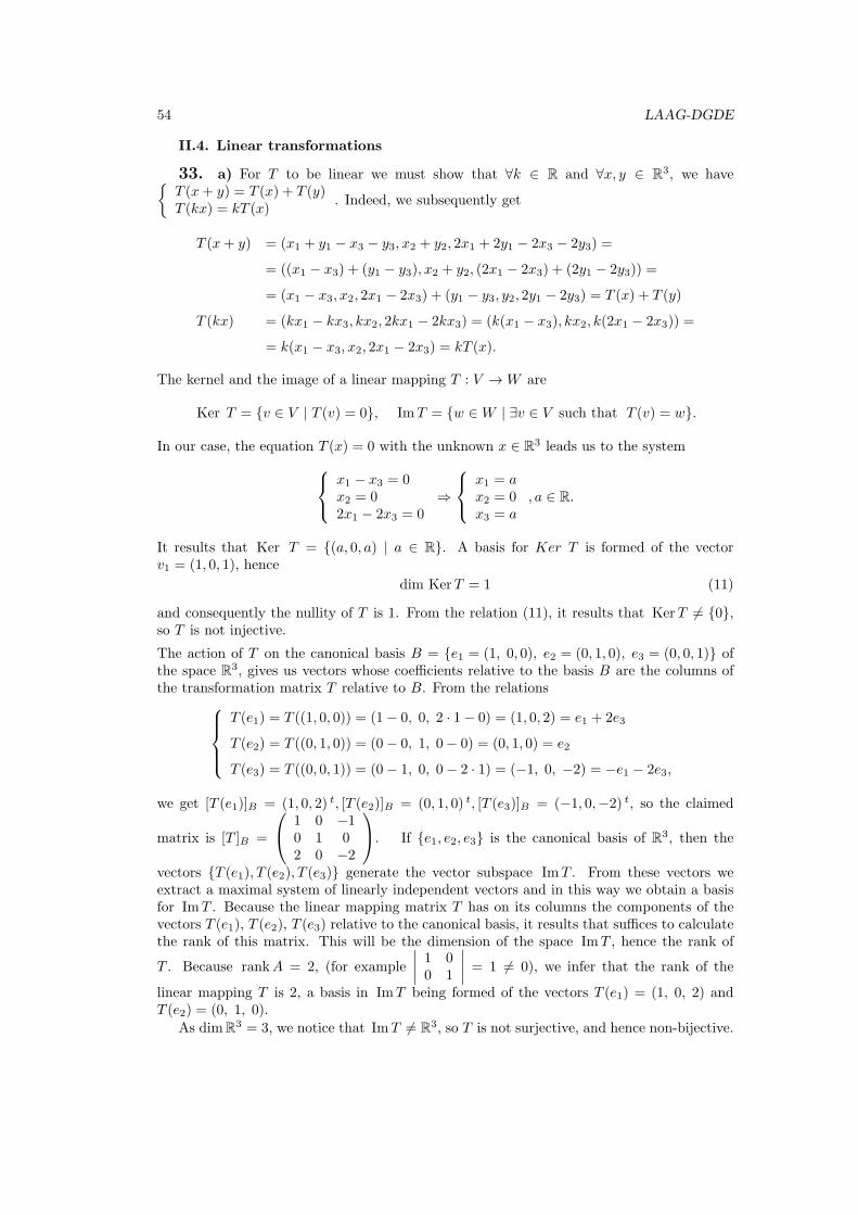
54 LAAG-DGDE
II.4. Linear transformations
33. a) For T to be linear we must show that ∀k ∈ R and ∀x, y ∈ R3, we have{T (x+ y) = T (x) + T (y)T (kx) = kT (x)
. Indeed, we subsequently get
T (x+ y) = (x1 + y1 − x3 − y3, x2 + y2, 2x1 + 2y1 − 2x3 − 2y3) =
= ((x1 − x3) + (y1 − y3), x2 + y2, (2x1 − 2x3) + (2y1 − 2y3)) =
= (x1 − x3, x2, 2x1 − 2x3) + (y1 − y3, y2, 2y1 − 2y3) = T (x) + T (y)
T (kx) = (kx1 − kx3, kx2, 2kx1 − 2kx3) = (k(x1 − x3), kx2, k(2x1 − 2x3)) =
= k(x1 − x3, x2, 2x1 − 2x3) = kT (x).
The kernel and the image of a linear mapping T : V →W are
Ker T = {v ∈ V | T (v) = 0}, ImT = {w ∈W | ∃v ∈ V such that T (v) = w}.
In our case, the equation T (x) = 0 with the unknown x ∈ R3 leads us to the system x1 − x3 = 0x2 = 02x1 − 2x3 = 0
⇒
x1 = ax2 = 0x3 = a
, a ∈ R.
It results that Ker T = {(a, 0, a) | a ∈ R}. A basis for Ker T is formed of the vectorv1 = (1, 0, 1), hence
dim KerT = 1 (11)
and consequently the nullity of T is 1. From the relation (11), it results that KerT = {0},so T is not injective.
The action of T on the canonical basis B = {e1 = (1, 0, 0), e2 = (0, 1, 0), e3 = (0, 0, 1)} ofthe space R3, gives us vectors whose coefficients relative to the basis B are the columns ofthe transformation matrix T relative to B. From the relations
T (e1) = T ((1, 0, 0)) = (1− 0, 0, 2 · 1− 0) = (1, 0, 2) = e1 + 2e3
T (e2) = T ((0, 1, 0)) = (0− 0, 1, 0− 0) = (0, 1, 0) = e2
T (e3) = T ((0, 0, 1)) = (0− 1, 0, 0− 2 · 1) = (−1, 0, −2) = −e1 − 2e3,
we get [T (e1)]B = (1, 0, 2) t, [T (e2)]B = (0, 1, 0) t, [T (e3)]B = (−1, 0,−2) t, so the claimed
matrix is [T ]B =
1 0 −10 1 02 0 −2
. If {e1, e2, e3} is the canonical basis of R3, then the
vectors {T (e1), T (e2), T (e3)} generate the vector subspace ImT . From these vectors weextract a maximal system of linearly independent vectors and in this way we obtain a basisfor ImT . Because the linear mapping matrix T has on its columns the components of thevectors T (e1), T (e2), T (e3) relative to the canonical basis, it results that suffices to calculatethe rank of this matrix. This will be the dimension of the space ImT , hence the rank of
T . Because rankA = 2, (for example
∣∣∣∣ 1 00 1
∣∣∣∣ = 1 = 0), we infer that the rank of the
linear mapping T is 2, a basis in ImT being formed of the vectors T (e1) = (1, 0, 2) andT (e2) = (0, 1, 0).
As dimR3 = 3, we notice that ImT = R3, so T is not surjective, and hence non-bijective.
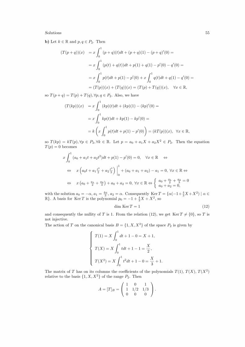
Solutions 55
b) Let k ∈ R and p, q ∈ P2. Then
(T (p+ q))(x) = x
∫ 1
0
(p+ q)(t)dt+ (p+ q)(1)− (p+ q)′(0) =
= x
∫ 1
0
(p(t) + q(t))dt+ p(1) + q(1)− p′(0)− q′(0) =
= x
∫ 1
0
p(t)dt+ p(1)− p′(0) + x
∫ 1
0
q(t)dt+ q(1)− q′(0) =
= (T (p))(x) + (T (q))(x) = (T (p) + T (q))(x), ∀x ∈ R,
so T (p+ q) = T (p) + T (q),∀p, q ∈ P2. Also, we have
(T (kp))(x) = x
∫ 1
0
(kp)(t)dt+ (kp)(1)− (kp)′(0) =
= x
∫ 1
0
kp(t)dt+ kp(1)− kp′(0) =
= k
(x
∫ 1
0
p(t)dt+ p(1)− p′(0)
)= (kT (p))(x), ∀x ∈ R,
so T (kp) = kT (p), ∀p ∈ P2, ∀k ∈ R. Let p = a0 + a1X + a2X2 ∈ P2. Then the equation
T (p) = 0 becomes
x
∫ 1
0
(a0 + a1t+ a2t2)dt+ p(1)− p′(0) = 0, ∀x ∈ R ⇔
⇔ x(a0t+ a1
t2
2 + a2t3
3
) ∣∣∣∣10
+ (a0 + a1 + a2)− a1 = 0, ∀x ∈ R ⇔
⇔ x(a0 +
a12 + a2
3
)+ a0 + a2 = 0, ∀x ∈ R ⇔
{a0 +
a12 + a2
3 = 0a0 + a2 = 0,
with the solution a0 = −α, a1 = 4α3 , a2 = α. Consequently KerT = {α(−1+ 4
3X+X2) | α ∈R}. A basis for KerT is the polynomial p0 = −1 + 4
3X +X2, so
dim KerT = 1 (12)
and consequently the nullity of T is 1. From the relation (12), we get KerT = {0}, so T isnot injective.
The action of T on the canonical basis B = {1, X,X2} of the space P2 is given by
T (1) = X
∫ 1
0
dt+ 1− 0 = X + 1,
T (X) = X
∫ 1
0
tdt+ 1− 1 =X
2,
T (X2) = X
∫ 1
0
t2dt+ 1− 0 =X
3+ 1.
The matrix of T has on its columns the coefficients of the polynomials T (1), T (X), T (X2)relative to the basis {1, X,X2} of the range P2. Then
A = [T ]B =
1 0 11 1/2 1/30 0 0
.
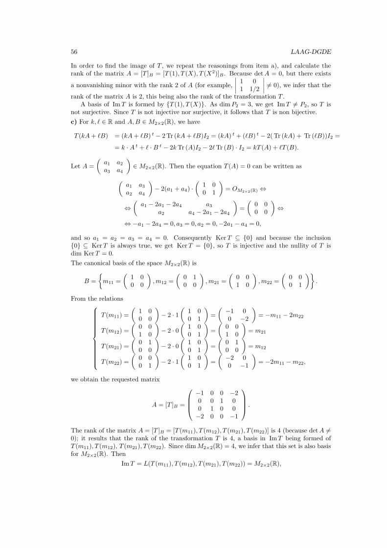
56 LAAG-DGDE
In order to find the image of T , we repeat the reasonings from item a), and calculate therank of the matrix A = [T ]B = [T (1), T (X), T (X2)]B. Because detA = 0, but there exists
a nonvanishing minor with the rank 2 of A (for example,
∣∣∣∣ 1 01 1/2
∣∣∣∣ = 0), we infer that the
rank of the matrix A is 2, this being also the rank of the transformation T .A basis of ImT is formed by {T (1), T (X)}. As dimP2 = 3, we get ImT = P2, so T is
not surjective. Since T is not injective nor surjective, it follows that T is non bijective.
c) For k, ℓ ∈ R and A,B ∈M2×2(R), we have
T (kA+ ℓB) = (kA+ ℓB) t − 2Tr (kA+ ℓB)I2 = (kA) t + (ℓB) t − 2(Tr (kA) + Tr (ℓB))I2 =
= k ·A t + ℓ ·B t − 2kTr (A)I2 − 2ℓTr (B) · I2 = kT (A) + ℓT (B).
Let A =
(a1 a2a3 a4
)∈M2×2(R). Then the equation T (A) = 0 can be written as
(a1 a3a2 a4
)− 2(a1 + a4) ·
(1 00 1
)= OM2×2(R) ⇔
⇔(a1 − 2a1 − 2a4 a3
a2 a4 − 2a1 − 2a4
)=
(0 00 0
)⇔
⇔ −a1 − 2a4 = 0, a3 = 0, a2 = 0,−2a1 − a4 = 0,
and so a1 = a2 = a3 = a4 = 0. Consequently KerT ⊆ {0} and because the inclusion{0} ⊆ KerT is always true, we get KerT = {0}, so T is injective and the nullity of T isdim KerT = 0.
The canonical basis of the space M2×2(R) is
B =
{m11 =
(1 00 0
),m12 =
(0 10 0
),m21 =
(0 01 0
),m22 =
(0 00 1
)}.
From the relations
T (m11) =
(1 00 0
)− 2 · 1
(1 00 1
)=
(−1 00 −2
)= −m11 − 2m22
T (m12) =
(0 01 0
)− 2 · 0
(1 00 1
)=
(0 01 0
)= m21
T (m21) =
(0 10 0
)− 2 · 0
(1 00 1
)=
(0 10 0
)= m12
T (m22) =
(0 00 1
)− 2 · 1
(1 00 1
)=
(−2 00 −1
)= −2m11 −m22,
we obtain the requested matrix
A = [T ]B =
−1 0 0 −20 0 1 00 1 0 0−2 0 0 −1
.
The rank of the matrix A = [T ]B = [T (m11), T (m12), T (m21), T (m22)] is 4 (because detA =0); it results that the rank of the transformation T is 4, a basis in ImT being formed ofT (m11), T (m12), T (m21), T (m22). Since dimM2×2(R) = 4, we infer that this set is also basisfor M2×2(R). Then
ImT = L(T (m11), T (m12), T (m21), T (m22)) =M2×2(R),
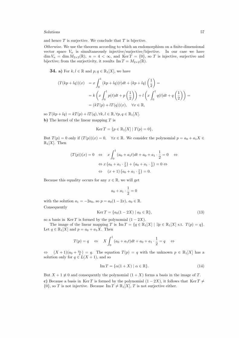
Solutions 57
and hence T is surjective. We conclude that T is bijective.
Otherwise. We use the theorem according to which an endomorphism on a finite-dimensionalvector space Vn is simultaneously injective/surjective/bijective. In our case we havedimVn = dimM2×2(R), n = 4 < ∞, and KerT = {0}, so T is injective, surjective andbijective; from the surjectivity, it results ImT =M2×2(R).
34. a) For k, l ∈ R and p, q ∈ R1[X], we have
(T (kp+ lq))(x) = x
∫ 1
0
(kp+ lq)(t)dt+ (kp+ lq)
(1
2
)=
= k
(x
∫ 1
0
p(t)dt+ p
(1
2
))+ l
(x
∫ 1
0
q(t)dt+ q
(1
2
))=
= (kT (p) + lT (q))(x), ∀x ∈ R,
so T (kp+ lq) = kT (p) + lT (q), ∀k, l ∈ R,∀p, q ∈ R1[X].
b) The kernel of the linear mapping T is
KerT = {p ∈ R1[X] | T (p) = 0},
But T (p) = 0 only if (T (p))(x) = 0, ∀x ∈ R. We consider the polynomial p = a0 + a1X ∈R1[X]. Then
(T (p))(x) = 0 ⇔ x
∫ 1
0
(a0 + a1t)dt+ a0 + a1 ·1
2= 0 ⇔
⇔ x(a0 + a1 · 1
2
)+(a0 + a1 · 1
2
)= 0 ⇔
⇔ (x+ 1)(a0 + a1 · 1
2
)= 0.
Because this equality occurs for any x ∈ R, we will get
a0 + a1 ·1
2= 0
with the solution a1 = −2a0, so p = a0(1− 2x), a0 ∈ R.Consequently
KerT = {a0(1− 2X) | a0 ∈ R}, (13)
so a basis in KerT is formed by the polynomial (1− 2X).The image of the linear mapping T is ImT = {q ∈ R1[X] | ∃p ∈ R1[X] s.t. T (p) = q}.
Let q ∈ R1[X] and p = a0 + a1X. Then
T (p) = q ⇔ X
∫ 1
0
(a0 + a1t)dt+ a0 + a1 ·1
2= q ⇔
⇔ (X + 1)(a0 +a12 ) = q. The equation T (p) = q with the unknown p ∈ R1[X] has a
solution only for q ∈ L(X + 1), and so
ImT = {α(1 +X) | α ∈ R}. (14)
But X + 1 ≡ 0 and consequently the polynomial (1 +X) forms a basis in the image of T .
c) Because a basis in KerT is formed by the polynomial (1− 2X), it follows that KerT ={0}, so T is not injective. Because ImT = R1[X], T is not surjective either.
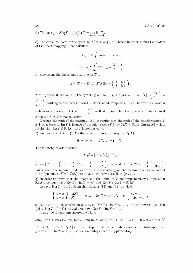
58 LAAG-DGDE
d) We have dimKer︸ ︷︷ ︸1
T + dim Im︸ ︷︷ ︸1
T = dimR1[X]︸ ︷︷ ︸2
.
e) The canonical basis of the space R1[X] is B = {1, X}, hence in order to find the matrixof the linear mapping T , we calculate
T (1) = X
∫ 1
0
dt+ 1 = X + 1
T (X) = X
∫ 1
0
tdt+1
2=X
2+
1
2.
In conclusion, the linear mapping matrix T is
A = [T ]B = [T (1), T (X)]B =
(1 1/21 1/2
).
T is injective if and only if the system given by T (a0 + a1X) = 0 ⇔ [T ] ·(a0a1
)=(
00
)(writing in the matrix form) is determined compatible. But, because the system
is homogeneous and detA =
∣∣∣∣ 1 1/21 1/2
∣∣∣∣ = 0, it follows that the system is undetermined
compatible, so T is not injective.Because the rank of the matrix A is 1, it results that the rank of the transformation T
is 1, so a basis in ImT is formed of a single vector (T (1) or T (X)). Since dimR1[X] = 2, itresults that ImT = R1[X], so T is not surjective.
f) We denote with B = {1, X} the canonical basis of the space R1[X] and
B′ = {q1 = 1− 2X, q2 = 1 +X}.
The following relation occurs
[T ]B′ = [B′]−1
B [T ]B [B′]B ,
where [B′]B =
(1 1−2 1
), [T ]B =
(1 1/21 1/2
), hence it results [T ]B
′ =
(0 00 3/2
).
Otherwise. The required matrix can be obtained setting on the columns the coefficients ofthe polynomials {T (q1), T (q2)} relative to the new basis B′ = {q1, q2}.g) In order to prove that the image and the kernel of T are supplementary subspaces inR1[X], we must have KerT ∩ ImT = {0} and KerT + ImT = R1[X].
Let p ∈ KerT ∩ ImT . From the relations (13) and (14) we yield{p = a0(1− 2X)p = α(1 +X)
⇔ a0 − 2a0X = α+ αX ⇔{a0 = α−2a0 = α
,
so a0 = α = 0. In conclusion p ≡ 0, so KerT ∩ ImT ⊆ {0}. As the reverse inclusion{0} ⊆ KerT ∩ ImT is trivial , we have KerT ∩ ImT = {0}.
Using the Grassmann theorem, we have
dim(KerT + ImT ) = dim KerT+dim ImT−dim(KerT ∩ ImT ) = 1+1−0 = 2 = dimR1[x].
As KerT + ImT ⊂ R1[X] and the subspace has the same dimension as the total space, weget KerT + ImT = R1[X]; so the two subspaces are supplementary.
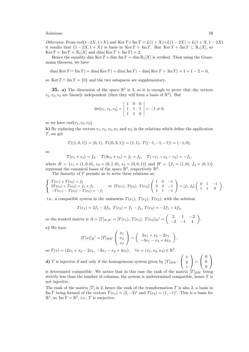
Solutions 59
Otherwise. From ind{1−2X, 1+X} and KerT+ImT = L(1 +X)+L(1− 2X) = L(1 +X, 1− 2X)it results that {1− 2X, 1 +X} is basis in KerT + ImT . But KerT + ImT ⊂ R1[X], soKerT + ImT = R1[X] and dim(KerT + ImT ) = 2.
Hence the equality dim KerT +dim ImT = dimR1[X] is verified. Then using the Grass-mann theorem, we have
dim(KerT ∩ ImT ) = dim(KerT ) + dim( ImT )− dim(KerT + ImT ) = 1 + 1− 2 = 0,
so KerT ∩ ImT = {0} and the two subspaces are supplementary.
35. a) The dimension of the space R3 is 3, so it is enough to prove that the vectorsv1, v2, v3 are linearly independent (then they will form a basis of R3). But
det[v1, v2, v3] =
∣∣∣∣∣∣1 0 01 1 11 1 0
∣∣∣∣∣∣ = −1 = 0,
so we have ind{v1, v2, v3}.b) By replacing the vectors v1, v2, v3, w1 and w2 in the relations which define the applicationT , we get
T ((1, 0, 1)) = (0, 1), T ((0, 3, 1)) = (1, 1), T ((−1,−1,−1)) = (−1, 0),
soT (e1 + e3) = f2, T (3e2 + e3) = f1 + f2, T (−e1 − e2 − e3) = −f1,
where B = {e1 = (1, 0, 0), e2 = (0, 1, 0), e3 = (0, 0, 1)} and B′ = {f1 = (1, 0), f2 = (0, 1)}represent the canonical bases of the space R3, respectively R2.
The linearity of T permits us to write these relations as:T (e1) + T (e3) = f23T (e2) + T (e3) = f1 + f2−T (e1)− T (e2)− T (e3) = −f1
⇔ [T (e1), T (e2), T (e3)]
1 0 −10 3 −11 1 −1
= [f1, f2]
(0 1 −11 1 0
),
i.e., a compatible system in the unknowns T (e1), T (e2), T (e3), with the solution
T (e1) = 2f1 − 3f2, T (e2) = f1 − f2, T (e3) = −2f1 + 4f2,
so the wanted matrix is A = [T ]B,B′ = [T (e1), T (e2), T (e3)]B′ =
(2 1 −2−3 −1 4
).
c) We have
[T (x)]B′ = [T ]BB′
x1x2x3
=
(2x1 + x2 − 2x3−3x1 − x2 + 4x3
),
so T (x) = (2x1 + x2 − 2x3, −3x1 − x2 + 4x3), ∀x = (x1, x2, x3) ∈ R3.
d) T is injective if and only if the homogeneous system given by [T ]BB′ ·
xyz
=
000
is determined compatible. We notice that in this case the rank of the matrix [T ]BB′ beingstrictly less than the number of columns, the system is undetermined compatible, hence T isnot injective.
The rank of the matrix [T ] is 2, hence the rank of the transformation T is also 2, a basis inImT being formed of the vectors T (e1) = (2,−3)t and T (e2) = (1,−1)t. This is a basis forR2, so ImT = R2, i.e., T is surjective.
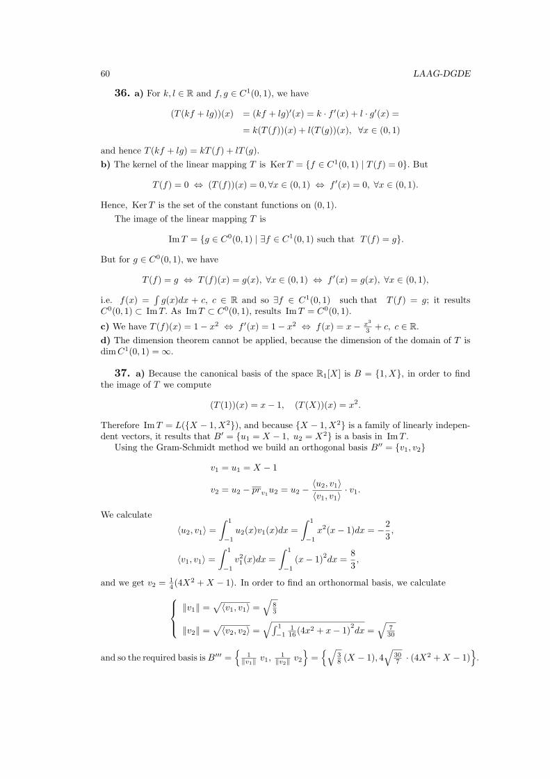
60 LAAG-DGDE
36. a) For k, l ∈ R and f, g ∈ C1(0, 1), we have
(T (kf + lg))(x) = (kf + lg)′(x) = k · f ′(x) + l · g′(x) =
= k(T (f))(x) + l(T (g))(x), ∀x ∈ (0, 1)
and hence T (kf + lg) = kT (f) + lT (g).
b) The kernel of the linear mapping T is KerT = {f ∈ C1(0, 1) | T (f) = 0}. But
T (f) = 0 ⇔ (T (f))(x) = 0, ∀x ∈ (0, 1) ⇔ f ′(x) = 0, ∀x ∈ (0, 1).
Hence, KerT is the set of the constant functions on (0, 1).
The image of the linear mapping T is
ImT = {g ∈ C0(0, 1) | ∃f ∈ C1(0, 1) such that T (f) = g}.
But for g ∈ C0(0, 1), we have
T (f) = g ⇔ T (f)(x) = g(x), ∀x ∈ (0, 1) ⇔ f ′(x) = g(x), ∀x ∈ (0, 1),
i.e. f(x) =∫g(x)dx + c, c ∈ R and so ∃f ∈ C1(0, 1) such that T (f) = g; it results
C0(0, 1) ⊂ ImT. As ImT ⊂ C0(0, 1), results ImT = C0(0, 1).
c) We have T (f)(x) = 1− x2 ⇔ f ′(x) = 1− x2 ⇔ f(x) = x− x3
3 + c, c ∈ R.d) The dimension theorem cannot be applied, because the dimension of the domain of T isdimC1(0, 1) = ∞.
37. a) Because the canonical basis of the space R1[X] is B = {1, X}, in order to findthe image of T we compute
(T (1))(x) = x− 1, (T (X))(x) = x2.
Therefore ImT = L({X − 1, X2}), and because {X − 1, X2} is a family of linearly indepen-dent vectors, it results that B′ = {u1 = X − 1, u2 = X2} is a basis in ImT .
Using the Gram-Schmidt method we build an orthogonal basis B′′ = {v1, v2}
v1 = u1 = X − 1
v2 = u2 − prv1u2 = u2 −⟨u2, v1⟩⟨v1, v1⟩
· v1.
We calculate
⟨u2, v1⟩ =∫ 1
−1
u2(x)v1(x)dx =
∫ 1
−1
x2(x− 1)dx = −2
3,
⟨v1, v1⟩ =∫ 1
−1
v21(x)dx =
∫ 1
−1
(x− 1)2dx =
8
3,
and we get v2 = 14 (4X
2 +X − 1). In order to find an orthonormal basis, we calculate∥v1∥ =
√⟨v1, v1⟩ =
√83
∥v2∥ =√⟨v2, v2⟩ =
√∫ 1
−1116 (4x
2 + x− 1)2dx =
√730
and so the required basis isB′′′ ={
1∥v1∥ v1,
1∥v2∥ v2
}={√
38 (X − 1), 4
√307 · (4X2 +X − 1)
}.
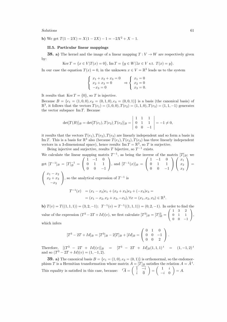
Solutions 61
b) We get T (1− 2X) = X(1− 2X)− 1 = −2X2 +X − 1.
II.5. Particular linear mappings
38. a) The kernel and the image of a linear mapping T : V →W are respectively givenby:
KerT = {x ∈ V |T (x) = 0}, ImT = {y ∈W |∃x ∈ V s.t. T (x) = y}.
In our case the equation T (x) = 0, in the unknown x ∈ V = R3 leads us to the system x1 + x2 + x3 = 0x2 + x3 = 0−x3 = 0
⇒
x1 = 0x2 = 0x3 = 0.
It results that KerT = {0}, so T is injective.
Because B = {e1 = (1, 0, 0), e2 = (0, 1, 0), e3 = (0, 0, 1)} is a basis (the canonical basis) ofR3, it follows that the vectors T (e1) = (1, 0, 0), T (e2) = (1, 1, 0), T (e3) = (1, 1,−1) generatesthe vector subspace ImT . Because
det[T (B)]B = det[T (e1), T (e2),T (e3)]B =
∣∣∣∣∣∣1 1 10 1 10 0 −1
∣∣∣∣∣∣ = −1 = 0,
it results that the vectors T (e1), T (e2), T (e3) are linearly independent and so form a basis inImT . This is a basis for R3 also (because T (e1), T (e2), T (e3) has three linearly independentvectors in a 3-dimensional space), hence results ImT = R3, so T is surjective.
Being injective and surjective, results T bijective, so T−1 exists.
We calculate the linear mapping matrix T−1, as being the inverse of the matrix [T ]B ; we
get [T−1]B = [T ]−1B =
1 −1 00 1 10 0 −1
, and [T−1(x)]B =
1 −1 00 1 10 0 −1
x1x2x3
= x1 − x2x2 + x3−x3
, so the analytical expression of T−1 is
T−1(x) = (x1 − x2)e1 + (x2 + x3)e2 + (−x3)e3 =
= (x1 − x2, x2 + x3,−x3), ∀x = (x1, x2, x3) ∈ R3.
b) T (v) = T ((1, 1, 1)) = (3, 2,−1); T−1(v) = T−1((1, 1, 1)) = (0, 2,−1). In order to find the
value of the expression (T 3 − 2T + Id)(v), we first calculate [T 3]B = [T ]3B =
1 3 20 1 10 0 −1
,
which infers
[T 3 − 2T + Id]B = [T 3]B − 2[T ]B + [Id]B =
0 1 00 0 −10 0 2
.
Therefore, [(T 3 − 2T + Id)(v)]B = [T 3 − 2T + Id]B(1, 1, 1)t = (1,−1, 2) t
and so (T 3 − 2T + Id)(v) = (1,−1, 2).
39. a) The canonical basis B = {e1 = (1, 0), e2 = (0, 1)} is orthonormal, so the endomor-phism T is a Hermitian transformation whose matrix A = [T ]B satisfies the relation A = A t.
This equality is satisfied in this case, because: tA =
(1 −ii 0
)=
(1 i−i 0
)= A.
62 LAAG-DGDE
b) Because a, b ∈ R, it results a = a and b = b, so we have A t =
(a z
z b
)=
(a zz b
)= A.
c) We have tA =
(ia −zz ib
)=
(−ia −zz −ib
)= −A, so the endomorphism T is skew-
Hermitian.
d) The endomorphism T is unitary if A · A∗ = A∗ · A = I2, where A∗ = tA. We
have A t =
(u v−¯v ¯u
)=
(u v−v u
)and hence A · A∗ =
(u −vv u
)·(
u v−v u
)=(
|u|2 + |v|2 00 |v|2 + |u|2
)=
(1 00 1
)= I2. Similarly, one can verify the equality
A∗ ·A = I2.
e) The real endomorphism T is called symmetric if its matrix A = [T ]B relative to thecanonical orthonormal basis B = {e1, e2} ⊂ R2 satisfies the relation A = tA. Obviously, inour case this relation holds true.
f) The endomorphism T is skew-symmetric because A = −A t (which can be easily be
checked). T is called complex structure ifA2 = −I2; we haveA2 =
(0 −11 0
)(0 −11 0
)=(
−1 00 −1
)= −I2. Because A · A t =
(0 −11 0
)(0 1−1 0
)=
(1 00 1
)= I2 and
similarly, A t ·A = I2. It results that T is an orthogonal endomorphism.
g) We have
A·A t =
(cosα − sinαsinα cosα
)·(
cosα sinα− sinα cosα
)=
(cos2 α+ sin2 α 0
0 sin2 α+ cos2 α
)= I2
and analogously, A t ·A = I2, so T is orthogonal.
h) The endomorphism T is called projection if A2 = A. But A2 =
(1/2 1/21/2 1/2
)= A, so T
is a projection.
i) T is nilpotent operator of order three if A3 = 0M3×3(R), equality which is verified.
40. a) We use the inner product ⟨A,B⟩=Tr ⟨A ·Bt⟩, ∀A,B ∈ M2(R). If the realendomorphism T has the property T = T ∗, i.e. ⟨TA,B⟩ = ⟨A, TB⟩, ∀A,B ∈ M2(R), thenT is called symmetric transformation.
In this case, using the trace properties Tr(C) = Tr(C t), T r(AB) = Tr(BA), we have⟨TA,B⟩ = ⟨A t, B⟩ = Tr⟨A t ·B t⟩ = Tr(BA) t = Tr(BA) = Tr(AB) = Tr(A t · B t)=⟨A,B t⟩ = ⟨A, TB⟩, so T is symmetric relative to the canonical inner product on M2×2(R).
b) We use the inner product ⟨f, g⟩ =∫ baf(x)g(x)dx, ∀f, g ∈ C0[a, b] ⊃ V .
Let f, g ∈ V . Using the integration by parts and the equalities f(a) = f(b), g(a) = g(b), weget:
⟨Tf, g⟩ =∫ ba(T (f)(x))g(x)dx =
∫ baf ′(x)g(x)dx = f(x)g(x)|ba −
∫ baf(x)g′(x)dx =
= f(b)g(b)− f(a)g(a)−∫ baf(x)(T (g)(x))dx = 0− ⟨f, Tg⟩ = −⟨f, Tg⟩,
hence the mapping is skew-symmetric relative to the canonical inner product on C0[a, b] ⊃ V .
41. a) Tv is linear if T (αx+ βy) = αT (x) + βT (y), ∀α, β ∈ R, ∀x, y ∈ V . We have
Tv(αx+ βy) = αx+ βy + v, αTv(x) + βTv(y) = α(x+ v) + β(y + v) = αx+ βy + αv + βv,
Solutions 63
so Tv is linear if and only if v = αv+βv, ∀α, β ∈ R ⇔ (α+β−1)v = 0, ∀α, β ∈ R, conditionwhich is equivalent to v = 0. Obviously, for v = 0, we get Tv = Id, the only case in whichTv is linear.
b) Let v = 0. It is known that T = Tv preserves the inner product if ∀x, y ∈ V we have
⟨Tx, Ty⟩ = ⟨x, y⟩ ⇔ ⟨x+ v, y + v⟩ = ⟨x, y⟩ ⇔
⇔ ⟨x, y⟩+ ⟨x, v⟩+ ⟨v, y⟩+ ⟨v, v⟩ = ⟨x, y⟩ ⇒ ⟨x, v⟩+ ⟨v, y⟩+ ⟨v, v⟩ = 0,
relation which must take place for any x, y ∈ V . But for x = y = v we get
3⟨v, v⟩ = 0 ⇔ 3∥v∥2 = 0 ⇔ ∥v∥ = 0 ⇔ v = 0,
in contradiction with the assumption v = 0; so T does not preserve the inner product. Also,T = Tv does not preserve the norm for v = 0, because
∥Tv(v)∥ = ∥2v∥ = 2∥v∥ = ∥v∥,
and so the relation ∥Tv(x)∥ = ∥x∥, ∀x ∈ V does not occur.
c) We notice that ∀y ∈ V , we have Tv(y − v) = y, so Tv is surjective. Also, we notice thatthe application T = Tv preserves the distance if d(Tv(x), Tv(y)) = d(x, y), ∀x, y ∈ V , whered(x, y) = ∥x− y∥,∀x, y ∈ V . We have
d(Tv(x), Tv(y)) = ∥T (x)− T (y)∥ = ∥(x+ v)− (y + v)∥ = ∥x− y∥ = d(x, y),
so T = Tv preserves the distance induced by the norm given by the inner product.
Remark. If || · || is any norm on V , it can be analogously proved that T = Tv preserves thedistance induced by || · ||.
II.6. Eigenvalues and eigenvectors. Diagonal form
42. a) We calculate the characteristic polynomial
P (λ) = det(A− λI3) =
∣∣∣∣∣∣2− λ 0 00 −λ 10 −1 −λ
∣∣∣∣∣∣ = −λ3 + 2λ2 − λ+ 2.
b) We solve the characteristic equation
P (λ) = 0 ⇔ −λ3 + 2λ2 − λ+ 2 = 0,
so the algebraic equation −(λ2 + 1)(λ − 2) = 0. The real roots of these equations are theeigenvalues of the matrix A and form the spectrum of the transformation T , σ(T ) = {2}.Because not all the roots of the polynomial P (λ) are real, it results that T is not Jordanizable,hence neither diagonalizable.
In this case σ(TC) = {2,−i,+i} ⊂ R.c) We notice that for λ = λ1 = 2 we have µa(λ 1) = 1, for λ = −i we have µa(−i) = 1, andfor λ = i we have µa(i) = 1.
For λ = λ1 = 2 the associated characteristic system is a system of linear equations whichhas as solutions the eigenvectors associated to the eigenvalues λ1 = 2. This system is:
(A− 2I3)(v) = 0 ⇔
0 0 00 −2 10 −1 −2
xyz
=
000
⇔{
−2y + z = 0−y − 2z = 0,
64 LAAG-DGDE
and has the solutions v = (x, y, z) = (t, 0, 0) = t(1, 0, 0), t ∈ R. Therefore Sλ1 = L(v1) , wherev1 = (1, 0, 0) is non null, so linearly independent, which form as basis in the eigenspace Sλ1 ,hence µg(λ1) = dim Sλ1 = 1.
We emphasize this, because λ2,3 = ±i /∈ R, λ2,3 are not eigenvalues of the endomorphismT . Yet for TC (the complexification of the morphism T ), and for the matrix A = [TC] ∈M3×3(C), the diagonalization is possible.
For λ = λ2 = −i, the associated characteristic system is:
(A+ iI3)v = 0 ⇔
2 + i 0 00 i 10 −1 i
xyz
=
000
⇔
(2 + i)x = 0iy + z = 0−y + iz = 0
and has the solutions v = (x, y, z) = (0, it, t) = t(0, i, 1), t ∈ C. Therefore Sλ2 = L(v2) ,where v2 = (0, i, 1) is non null, so linearly independent, and form a basis in the eigenspaceSλ2 , hence µg(λ2) = dimSλ2 = 1.
For λ = λ3 = i, the associated characteristic system is:
(A− iI3)v = 0 ⇔
2− i 0 00 −i 10 −1 −i
xyz
=
000
⇔
(2− i)x = 0−iy + z = 0−y − iz = 0
and has the solutions v = (x, y, z) = (0,−it, t) = t(0,−i, 1), t ∈ C. Therefore Sλ3 = L(v3), where v3 = (0,−i, 1) is non null, hence linearly independent, which form a basis in theeigenspace Sλ3 , hence µg(λ3) = dim Sλ3
= 1.
We notice that µa(λ) = µg(λ), for any λ = λ1, λ2, λ3, so the transformation TC is diagonal-izable.
43. a) We calculate the characteristic polynomial
P (λ) = det(A− λI) =
∣∣∣∣∣∣3− λ 0 00 2− λ 10 0 2− λ
∣∣∣∣∣∣ = −λ3 + 7λ2 − 16λ+ 12.
We solve the characteristic equation
P (λ) = 0 ⇔ −λ3 + 7λ2 − 16λ+ 12 = 0,
so the algebraic equation −(λ− 3)(λ− 2)2 = 0. The eigenvalues of the matrix A are the realroots of this equations and because all the roots are real, the spectrum is σ(T ) = σ(TC) ={3, 2, 2}. Because σ(TC) ⊂ R, it results that T is Jordanizable.
For λ = λ1 = 3 and λ = λ2 = 2 we have µa(3) = 1, respectively µa(2) = 2.For λ = λ1 = 3, the associated characteristic system is
(A− 3I)v = 0 ⇔
0 0 00 −1 10 0 −1
abc
=
000
⇔{
−b+ c = 0−c = 0,
and has the solutions (a, b, c) = (t, 0, 0) = t(1, 0, 0), t ∈ R. Therefore a basis in the eigenspaceSλ1 is the non null generator (hence linearly independent) v1 = (1, 0, 0), hence it resultsµg(λ1) = dim Sλ1 = 1 = µa(λ1).
For λ = λ2 = 2, the associated characteristic system is:
(A− 2I)v = 0 ⇔
1 0 00 0 10 0 0
abc
=
000
⇔{a = 0c = 0,
Solutions 65
and has the solutions v = (a, b, c) = (0, t, 0) = t(0, 1, 0), t ∈ R. We conclude that the vectorv2 = (0, 1, 0) t provides a basis for Sλ2 . Hence it results that µg(λ2) = dimSλ2 = 1.
Because for λ = λ2 we have µg(λ2) = 1 = µa(λ2) = 2 it results that the endomorphismT is not diagonalizable.
b) We calculate the characteristic polynomial
P (λ) = det(A− λI3) =
∣∣∣∣∣∣7− λ 4 −14 7− λ −1−4 −4 4− λ
∣∣∣∣∣∣ = −λ3 + 18λ2 − 81λ+ 108.
We solve the characteristic equation
P (λ) = 0 ⇔ −λ3 + 18λ2 − 81λ+ 108 = 0,
so the algebraic equation −(λ−3)2(λ−12) = 0. The eigenvalues of the matrix A are the rootsof this equations and because all of them are real, the spectrum is σ(T ) = σ(TC) = {12, 3, 3}.Because σ(TC) ⊂ R, it results that T is Jordanizable.
For λ = λ1 = 12 and λ = λ2 = 3 we have µa(λ1) = 1, respectively µa(λ2) = 2.For λ = λ1 = 12 the associated characteristic system is
(A− 12I)v = 0 ⇔
−5 4 −14 −5 −1−4 −4 −8
abc
=
000
⇔
−5a+ 4b− c = 04a− 5b− c = 0−4a− 4b− 8c = 0
and has the solutions v = (a, b, c) = (t, t,−t) = t(1, 1,−1), t ∈ R. Therefore a basis in theeigenspace Sλ1 is the vector v1 = (1, 1,−1), hence µg(λ1) = dimSλ1 = 1 = µa(λ1).
For λ = λ2 = 3 the associated characteristic system is
(A− 3I)v = 0 ⇔
4 4 −14 4 −1−4 −4 1
abc
=
000
⇔ 4a+ 4b− c = 0
and has the solutions v = (a, b, c) = (α, β, 4α + 4β) = α(1, 0, 4) + β(0, 1, 4). In conclusion,a basis in Sλ2 is formed of the vectors v2 = (1, 0, 4) and v3 = (0, 1, 4), hence µg(λ2) =dimSλ2 = 2 = µa(λ2).
Since µa(λ1) = µg(λ1)(= 1) and µa(λ2) = µg(λ2)(= 2), the endomorphism T is diagonaliz-able.
The basis B′ of the space R3 relative to which the endomorphism matrix T is diagonal, isformed of the vectors (eigenvectors) of the bases of eigenspaces of T , i.e. B′ = {v1, v2, v3}.In conclusion, the endomorphism T is diagonalizable, and admits the following diagonalizingmatrix and the diagonal matrix, respectively
C = [v1, v2, v3]B =
1 1 01 0 1−1 4 4
, D =
12 0 00 3 00 0 3
.
We verify the relation D = C−1AC in the form CD = AC. We have
C ·D =
1 1 01 0 1−1 4 4
12 0 00 3 00 0 3
=
12 3 012 0 3−12 12 12
;
A · C =
7 4 −14 7 −1−4 −4 4
1 1 01 0 1−1 4 4
=
12 3 012 0 3−12 12 12
= CD.
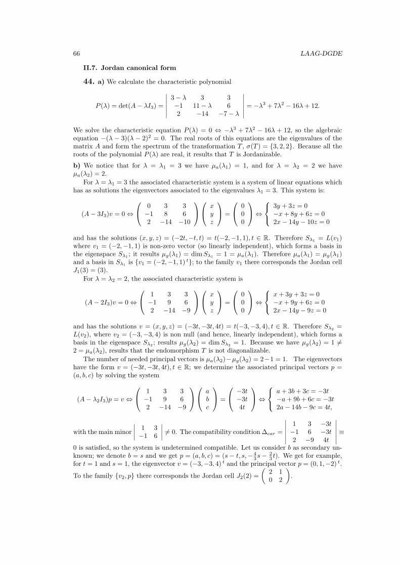
66 LAAG-DGDE
II.7. Jordan canonical form
44. a) We calculate the characteristic polynomial
P (λ) = det(A− λI3) =
∣∣∣∣∣∣3− λ 3 3−1 11− λ 62 −14 −7− λ
∣∣∣∣∣∣ = −λ3 + 7λ2 − 16λ+ 12.
We solve the characteristic equation P (λ) = 0 ⇔ −λ3 + 7λ2 − 16λ + 12, so the algebraicequation −(λ − 3)(λ − 2)2 = 0. The real roots of this equations are the eigenvalues of thematrix A and form the spectrum of the transformation T , σ(T ) = {3, 2, 2}. Because all theroots of the polynomial P (λ) are real, it results that T is Jordanizable.
b) We notice that for λ = λ1 = 3 we have µa(λ1) = 1, and for λ = λ2 = 2 we haveµa(λ2) = 2.
For λ = λ1 = 3 the associated characteristic system is a system of linear equations whichhas as solutions the eigenvectors associated to the eigenvalues λ1 = 3. This system is:
(A− 3I3)v = 0 ⇔
0 3 3−1 8 62 −14 −10
xyz
=
000
⇔
3y + 3z = 0−x+ 8y + 6z = 02x− 14y − 10z = 0
and has the solutions (x, y, z) = (−2t,−t, t) = t(−2,−1, 1), t ∈ R. Therefore Sλ1 = L(v1)where v1 = (−2,−1, 1) is non-zero vector (so linearly independent), which forms a basis inthe eigenspace Sλ1 ; it results µg(λ1) = dimSλ1 = 1 = µa(λ1). Therefore µa(λ1) = µg(λ1)and a basis in Sλ1 is {v1 = (−2,−1, 1) t}; to the family v1 there corresponds the Jordan cellJ1(3) = (3).
For λ = λ2 = 2, the associated characteristic system is
(A− 2I3)v = 0 ⇔
1 3 3−1 9 62 −14 −9
xyz
=
000
⇔
x+ 3y + 3z = 0−x+ 9y + 6z = 02x− 14y − 9z = 0
and has the solutions v = (x, y, z) = (−3t,−3t, 4t) = t(−3,−3, 4), t ∈ R. Therefore Sλ2 =L(v2), where v2 = (−3,−3, 4) is non null (and hence, linearly independent), which forms abasis in the eigenspace Sλ2 ; results µg(λ2) = dimSλ2 = 1. Because we have µg(λ2) = 1 =2 = µa(λ2), results that the endomorphism T is not diagonalizable.
The number of needed principal vectors is µa(λ2)−µg(λ2) = 2−1 = 1. The eigenvectorshave the form v = (−3t,−3t, 4t), t ∈ R; we determine the associated principal vectors p =(a, b, c) by solving the system
(A− λ2I3)p = v ⇔
1 3 3−1 9 62 −14 −9
abc
=
−3t−3t4t
⇔
a+ 3b+ 3c = −3t−a+ 9b+ 6c = −3t2a− 14b− 9c = 4t,
with the main minor
∣∣∣∣ 1 3−1 6
∣∣∣∣ = 0. The compatibility condition ∆car =
∣∣∣∣∣∣1 3 −3t−1 6 −3t2 −9 4t
∣∣∣∣∣∣ ≡0 is satisfied, so the system is undetermined compatible. Let us consider b as secondary un-known; we denote b = s and we get p = (a, b, c) = (s− t, s,− 4
3s−23 t). We get for example,
for t = 1 and s = 1, the eigenvector v = (−3,−3, 4) t and the principal vector p = (0, 1,−2) t.
To the family {v2, p} there corresponds the Jordan cell J2(2) =
(2 10 2
).
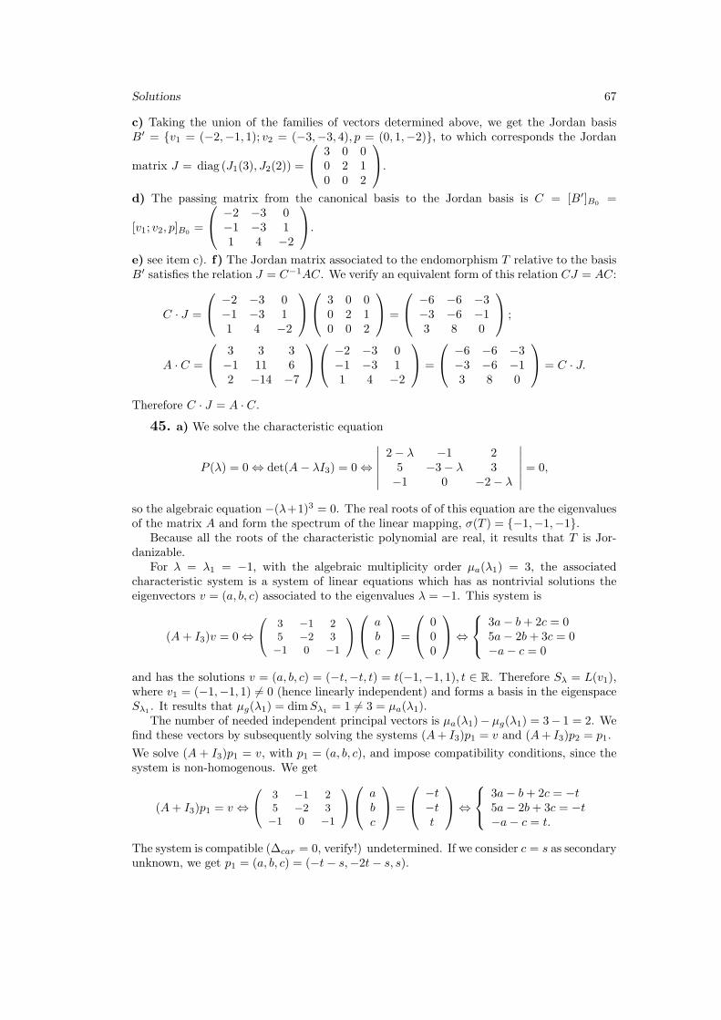
Solutions 67
c) Taking the union of the families of vectors determined above, we get the Jordan basisB′ = {v1 = (−2,−1, 1); v2 = (−3,−3, 4), p = (0, 1,−2)}, to which corresponds the Jordan
matrix J = diag (J1(3), J2(2)) =
3 0 00 2 10 0 2
.
d) The passing matrix from the canonical basis to the Jordan basis is C = [B′]B0 =
[v1; v2, p]B0 =
−2 −3 0−1 −3 11 4 −2
.
e) see item c). f) The Jordan matrix associated to the endomorphism T relative to the basisB′ satisfies the relation J = C−1AC. We verify an equivalent form of this relation CJ = AC:
C · J =
−2 −3 0−1 −3 11 4 −2
3 0 00 2 10 0 2
=
−6 −6 −3−3 −6 −13 8 0
;
A · C =
3 3 3−1 11 62 −14 −7
−2 −3 0−1 −3 11 4 −2
=
−6 −6 −3−3 −6 −13 8 0
= C · J.
Therefore C · J = A · C.
45. a) We solve the characteristic equation
P (λ) = 0 ⇔ det(A− λI3) = 0 ⇔
∣∣∣∣∣∣2− λ −1 25 −3− λ 3−1 0 −2− λ
∣∣∣∣∣∣ = 0,
so the algebraic equation −(λ+1)3 = 0. The real roots of of this equation are the eigenvaluesof the matrix A and form the spectrum of the linear mapping, σ(T ) = {−1,−1,−1}.
Because all the roots of the characteristic polynomial are real, it results that T is Jor-danizable.
For λ = λ1 = −1, with the algebraic multiplicity order µa(λ1) = 3, the associatedcharacteristic system is a system of linear equations which has as nontrivial solutions theeigenvectors v = (a, b, c) associated to the eigenvalues λ = −1. This system is
(A+ I3)v = 0 ⇔
3 −1 25 −2 3−1 0 −1
a
bc
=
000
⇔
3a− b+ 2c = 05a− 2b+ 3c = 0−a− c = 0
and has the solutions v = (a, b, c) = (−t,−t, t) = t(−1,−1, 1), t ∈ R. Therefore Sλ = L(v1),where v1 = (−1,−1, 1) = 0 (hence linearly independent) and forms a basis in the eigenspaceSλ1 . It results that µg(λ1) = dimSλ1 = 1 = 3 = µa(λ1).
The number of needed independent principal vectors is µa(λ1)− µg(λ1) = 3− 1 = 2. Wefind these vectors by subsequently solving the systems (A+ I3)p1 = v and (A+ I3)p2 = p1.
We solve (A + I3)p1 = v, with p1 = (a, b, c), and impose compatibility conditions, since thesystem is non-homogenous. We get
(A+ I3)p1 = v ⇔
3 −1 25 −2 3−1 0 −1
a
bc
=
−t−tt
⇔
3a− b+ 2c = −t5a− 2b+ 3c = −t−a− c = t.
The system is compatible (∆car = 0, verify!) undetermined. If we consider c = s as secondaryunknown, we get p1 = (a, b, c) = (−t− s,−2t− s, s).
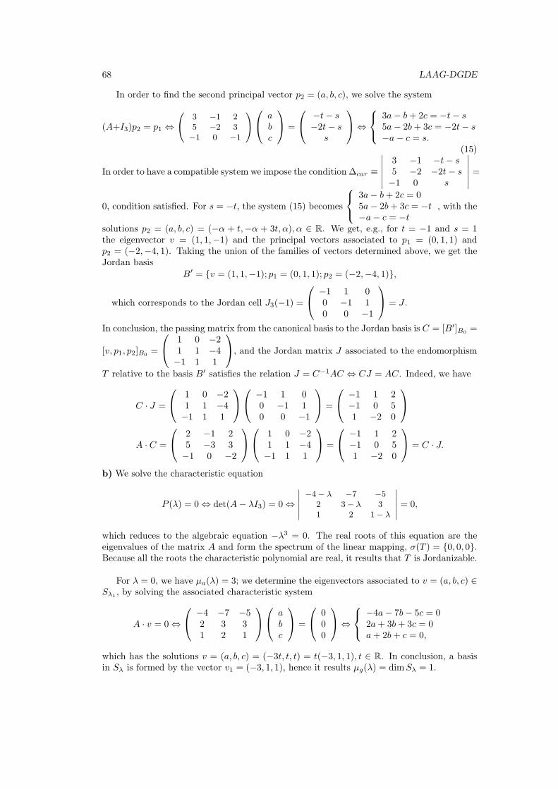
68 LAAG-DGDE
In order to find the second principal vector p2 = (a, b, c), we solve the system
(A+I3)p2 = p1 ⇔
3 −1 25 −2 3−1 0 −1
a
bc
=
−t− s−2t− s
s
⇔
3a− b+ 2c = −t− s5a− 2b+ 3c = −2t− s−a− c = s.
(15)
In order to have a compatible system we impose the condition ∆car ≡
∣∣∣∣∣∣3 −1 −t− s5 −2 −2t− s−1 0 s
∣∣∣∣∣∣ =0, condition satisfied. For s = −t, the system (15) becomes
3a− b+ 2c = 05a− 2b+ 3c = −t−a− c = −t
, with the
solutions p2 = (a, b, c) = (−α + t,−α + 3t, α), α ∈ R. We get, e.g., for t = −1 and s = 1the eigenvector v = (1, 1,−1) and the principal vectors associated to p1 = (0, 1, 1) andp2 = (−2,−4, 1). Taking the union of the families of vectors determined above, we get theJordan basis
B′ = {v = (1, 1,−1); p1 = (0, 1, 1); p2 = (−2,−4, 1)},
which corresponds to the Jordan cell J3(−1) =
−1 1 00 −1 10 0 −1
= J .
In conclusion, the passing matrix from the canonical basis to the Jordan basis is C = [B′]B0 =
[v, p1, p2]B0 =
1 0 −21 1 −4−1 1 1
, and the Jordan matrix J associated to the endomorphism
T relative to the basis B′ satisfies the relation J = C−1AC ⇔ CJ = AC. Indeed, we have
C · J =
1 0 −21 1 −4−1 1 1
−1 1 00 −1 10 0 −1
=
−1 1 2−1 0 51 −2 0
A · C =
2 −1 25 −3 3−1 0 −2
1 0 −21 1 −4−1 1 1
=
−1 1 2−1 0 51 −2 0
= C · J.
b) We solve the characteristic equation
P (λ) = 0 ⇔ det(A− λI3) = 0 ⇔
∣∣∣∣∣∣−4− λ −7 −5
2 3− λ 31 2 1− λ
∣∣∣∣∣∣ = 0,
which reduces to the algebraic equation −λ3 = 0. The real roots of this equation are theeigenvalues of the matrix A and form the spectrum of the linear mapping, σ(T ) = {0, 0, 0}.Because all the roots the characteristic polynomial are real, it results that T is Jordanizable.
For λ = 0, we have µa(λ) = 3; we determine the eigenvectors associated to v = (a, b, c) ∈Sλ1 , by solving the associated characteristic system
A · v = 0 ⇔
−4 −7 −52 3 31 2 1
abc
=
000
⇔
−4a− 7b− 5c = 02a+ 3b+ 3c = 0a+ 2b+ c = 0,
which has the solutions v = (a, b, c) = (−3t, t, t) = t(−3, 1, 1), t ∈ R. In conclusion, a basisin Sλ is formed by the vector v1 = (−3, 1, 1), hence it results µg(λ) = dimSλ = 1.
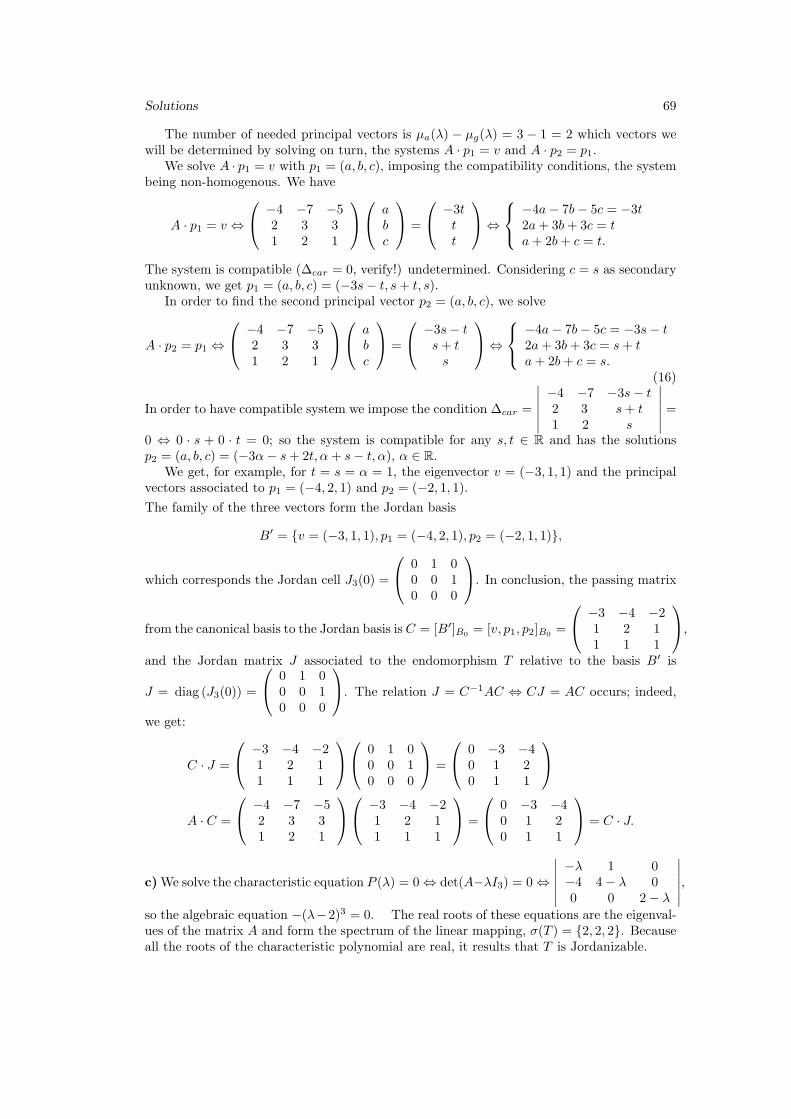
Solutions 69
The number of needed principal vectors is µa(λ) − µg(λ) = 3 − 1 = 2 which vectors wewill be determined by solving on turn, the systems A · p1 = v and A · p2 = p1.
We solve A · p1 = v with p1 = (a, b, c), imposing the compatibility conditions, the systembeing non-homogenous. We have
A · p1 = v ⇔
−4 −7 −52 3 31 2 1
abc
=
−3ttt
⇔
−4a− 7b− 5c = −3t2a+ 3b+ 3c = ta+ 2b+ c = t.
The system is compatible (∆car = 0, verify!) undetermined. Considering c = s as secondaryunknown, we get p1 = (a, b, c) = (−3s− t, s+ t, s).
In order to find the second principal vector p2 = (a, b, c), we solve
A · p2 = p1 ⇔
−4 −7 −52 3 31 2 1
abc
=
−3s− ts+ ts
⇔
−4a− 7b− 5c = −3s− t2a+ 3b+ 3c = s+ ta+ 2b+ c = s.
(16)
In order to have compatible system we impose the condition ∆car =
∣∣∣∣∣∣−4 −7 −3s− t2 3 s+ t1 2 s
∣∣∣∣∣∣ =0 ⇔ 0 · s + 0 · t = 0; so the system is compatible for any s, t ∈ R and has the solutionsp2 = (a, b, c) = (−3α− s+ 2t, α+ s− t, α), α ∈ R.
We get, for example, for t = s = α = 1, the eigenvector v = (−3, 1, 1) and the principalvectors associated to p1 = (−4, 2, 1) and p2 = (−2, 1, 1).
The family of the three vectors form the Jordan basis
B′ = {v = (−3, 1, 1), p1 = (−4, 2, 1), p2 = (−2, 1, 1)},
which corresponds the Jordan cell J3(0) =
0 1 00 0 10 0 0
. In conclusion, the passing matrix
from the canonical basis to the Jordan basis is C = [B′]B0 = [v, p1, p2]B0 =
−3 −4 −21 2 11 1 1
,
and the Jordan matrix J associated to the endomorphism T relative to the basis B′ is
J = diag (J3(0)) =
0 1 00 0 10 0 0
. The relation J = C−1AC ⇔ CJ = AC occurs; indeed,
we get:
C · J =
−3 −4 −21 2 11 1 1
0 1 00 0 10 0 0
=
0 −3 −40 1 20 1 1
A · C =
−4 −7 −52 3 31 2 1
−3 −4 −21 2 11 1 1
=
0 −3 −40 1 20 1 1
= C · J.
c)We solve the characteristic equation P (λ) = 0 ⇔ det(A−λI3) = 0 ⇔
∣∣∣∣∣∣−λ 1 0−4 4− λ 00 0 2− λ
∣∣∣∣∣∣,so the algebraic equation −(λ−2)3 = 0. The real roots of these equations are the eigenval-ues of the matrix A and form the spectrum of the linear mapping, σ(T ) = {2, 2, 2}. Becauseall the roots of the characteristic polynomial are real, it results that T is Jordanizable.
70 LAAG-DGDE
For λ = 2, with the algebraic multiplicity order µa(λ) = 3, the associated characteristicsystem is a system of linear equations which has as nontrivial solutions the eigenvectorsv = (a, b, c) associated to the eigenvalues λ = 2. This system is
(A− 2I3)v = 0 ⇔
−2 1 0−4 2 00 0 0
abc
=
000
⇔
−2a+ b = 0−4a+ 2b = 00 = 0
and has the solutions v = (a, b, c) = (t, 2t, s) = t(1, 2, 0) + s(0, 0, 1), s, t ∈ R. In conclusion, abasis in Sλ1 is formed by the vectors v1 = (1, 2, 0) and v2 = (0, 0, 1), hence results µg(λ1) =dimSλ1 = 2.
The number of needed principal vectors is µa(λ1) − µg(λ1) = 3 − 2 = 1, which are thesolutions of the system (A − 2I3)p = v. We solve this system, imposing the compatibilityconditions, the system being non-homogenous. Denoting p = (a, b, c), the system can bewritten as
(A− 2I3)p = v ⇔
−2 1 0−4 2 00 0 0
abc
=
t2ts
⇔
−2a+ b = t−4a+ 2b = 2t0 = s.
In order to have a compatible system, we impose the conditions ∆car1 =
∣∣∣∣ 1 t2 2t
∣∣∣∣ = 0 and
∆car2 =
∣∣∣∣ 1 t0 s
∣∣∣∣ = 0, hence results that we must have s = 0.
Let us consider a and c as secondary unknowns and denote a = α and c = β; then thesolution is p = (a, b, c) = (α, t+ 2α, β).
E.g., for t = 1, s = 0, α = 1 and β = 2, we get the eigenvector v1 = (1, 2, 0) and theprincipal associated vector p1 = (1, 3, 2). The second eigenvector will be chosen such thats = 0; e.g., for t = 1, s = −1, we get v2 = (1, 2,−1). Taking the union of the families ofvectors determined above, we get the Jordan basis
B′ = {v1 = (1, 2, 0), p1 = (1, 3, 2); v2 = (1, 2,−1)},
so the passing matrix from the canonical basis to the Jordan basis is C = [B′]B0 = [v1, p1; v2]B0 = 1 1 12 3 20 2 −1
. The Jordan matrix J associated to the endomorphism T relative to the
basis B′ is J = diag (J2(2), J1(2)) =
2 1 00 2 00 0 2
. The relation J = C−1AC ⇔ CJ = AC
occurs; indeed, we get
C · J =
1 1 12 3 20 2 −1
2 1 00 2 00 0 2
=
2 3 24 8 40 4 −2
A · C =
0 1 0−4 4 00 0 2
1 1 12 3 20 2 −1
=
2 3 24 8 40 4 −2
= C · J.
d) The eigenspace associated to distinct eigenvalues λ = 0 (µa(λ) = 4) is Sλ=0 = L({f1 =(1,−2, 1,−6)t, f2 = (0, 0, 1,−1)t}). Therefore the geometric multiplicity is µg(λ) = 2(< 4).We determine the 4 − 2 = 2 principal vectors by solving the system (A − 0I4)p = v, wherev = af1+ bf2. Choosing the principal minor at the intersection of the second and third rows
Solutions 71
with the first two columns, the compatibility of secondary equations 2 and 4 is identicallysatisfied, and the solutions are of type p = (s, a − 2s, b − t − 5s, t)t. For s = t = b =0, a = 1 it results v1 = (1,−2, 1,−6)t, p1 = (0, 1, 0, 0)t, and for s = t = a = 0, b = 1 weget v2 = (0, 0, 1,−1)t, p2 = (0, 0, 1, 0)t. The two families of vectors accordingly correspondto two Jordan cells of type J2(0) in the Jordan matrix J . The Jordan basis is hence B′ =
{v1, p1; v2, p2}, the Jordanizing matrix is C = [B′]B =
1 0 0 0−2 1 0 01 0 1 1−6 0 −1 0
and the Jordan
matrix associated to it, is J = diag (J2(0), J2(0)).
e) The two distinct eigenvalues are σ(A) = {λ1 = −1, λ2 = 2} with algebraic multiplicitiesµ1 = 1, µ2 = 2 respectively. For λ1 = −1 we have Sλ1 = L(v1 = (1, 1, 1)t), so the algebraicand geometric multiplicities are pairwise equal, and B1 = {v1} is a basis for the eigenspaceSλ1 . For λ2 = 2, we have Sλ2 = L(v2 = (0, 1, 1)t), so the geometric multiplicity is1 < µ2 = 2. We determine a principal vector p by solving the linear system (A− 2I3)p = v,where v = (0, t, t)t. The compatibility condition of the non-homogenous system is identicallysatisfied and we get the solution p = (0, s, s+ t)t; choosing t = 1, s = 0 leads to the family ofvectors B2 = {v2 = (0, 1, 1)t, p2 = (0, 0, 1)t}, a basis for the invariant subspace associated tothe eigenvalues λ2 = 2. Then the Jordan basis is B′ = B1∪B2 = {v1; v2, p2}, the Jordanizing
matrix is C = [B′]B =
1 0 01 1 01 1 1
and the Jordan matrix, J = diag (J1(−1), J2(2)).
46. We present the Jordanization algorithm based on the sequence of kernels method.
• We determine the distinct complex roots ρ(A) = {λ1, . . . , λp} of the characteristicpolynomial P (λ) = det(A − λIn) of the matrix A of the endomorphism T ∈ End(V )(dimK V = n).
• If ρ(A) ⊂ K, then T is not Jordanizable, and the algorithm stops. In the other case,T admits the canonic Jordan form and the algorithm continues.
• For each distinct eigenvalue λ = λi (i = 1, p) whose algebraic multiplicity is denotedby µi, we proceed as follows:
i) we determine a basis for the eigenspace Si = Ker (T − λId). If dimSi = µi, then wedenote this basis with Bi (to this, in the Jordan matrix there corresponds the blockdiag (λi, . . . , λi) of order µi) and we pass to the subsequent distinct eigenvalue. In thecontrary case, we proceed with the next item.
ii) we denote τ = T − λId, M = [τ ] = A− λIn and Kj = Ker (τ j). We determine themaximal order of the Jordan cell which is associated to the eigenvalue λ (i.e., the orderof nilpotency) as the natural number s ≥ 2 for which K1 ⊂ K2 ⊂ · · · ⊂ Ks = Ks+1 =Ks+2 = . . . .
iii) we subsequently decompose the bases βj of the subspaces Kj (j = 1, s), as follows:
βs = βs−1 ∪ Cs
βs−1 = βs−2 ∪ τ(Cs) ∪ Cs−1
βs−2 = βs−3 ∪ τ2(Cs) ∪ τ(Cs−1) ∪ Cs−2
. . .
β2 = β1 ∪ τs−2(Cs) ∪ τs−3(Cs−1) ∪ . . . ∪ τ(C3) ∪ C2
β1 = g� ∪ τs−1(Cs) ∪ τs−2(Cs−1) ∪ . . . ∪ τ2(C3) ∪ τ(C2) ∪ C1
72 LAAG-DGDE
where Cs, Cs−1, . . . C1 vectors sets (not all empty) constructed in order to fill the pre-ceding unions to the bases βs, . . . β1, respectively. For each k ∈ 1, s and each vectorpk ∈ Ck, we construct the family
{v = τk−1(p), τk−2(p), . . . , τ(p), p},
formed of k vectors (v= eigenvector and k − 1 principal vectors for k ≥ 2 and theeigenvector v = p for k = 1), to which in the Jordan matrix J there corresponds theJordan cell Jk(λ). We denote with Bi the union of these families. This is a basis forthe invariant subspace Ks (Ks ⊃ K1 = S1) associated to the eigenvalue λi.
• We build the Jordan basis B′ = B1 ∪ · · · ∪ Bp and the passing matrix to this basis,C = [B′]B . We build the Jordan matrix J = [T ]B′ associated to the endomorphismT , putting on the diagonal the blocks/cells associated to the families of vectors whichform B′, according to the order of their occurrence within the new basis B′.
• We verify the relation J = C−1AC in its equivalent form CJ = AC.
a) For the unique distinct eigenvalue λ = −1 (µ = 3), we get M2 = 03,M3 = 0, so s = 3 and
K3 = R3. Because K2 = L({(1, 0,−2), (0, 1, 1)} ∋ e3 = (0, 0, 1), we choose C3 = {p = e3}.Then we have
β3 = β2 ∪ {p = e3}β2 = β1 ∪ τ(e3) ∪ g�β1 = g� ∪ τ2(e3) ∪ g� .
The family of vectors
B′ = B1 = {v =M2e3 = (1, 1,−1)t, p1 =Me3 = (2, 3,−1)t, p2 = e3 = (0, 0, 1)}
is the basis of the invariant subspace K3 = R3 and represent a Jordan basis of the en-domorphism T . To it there corresponds the matrix of change of basis C = [v, p1, p2]B = 1 2 0
1 3 0−1 −1 1
and the Jordan matrix J = J3(−1). We notice that by choosing p =
(−2,−4, 1)t ∈ K2, we get the Jordan basis which was determined in problem 45-a),
B′ = {v =M2p = (1, 1,−1)t,Mp = (0, 1, 1)t, p = (−2,−4, 1)t}.
b) For the unique distinct eigenvalue λ = 0 we get M2 = 03,M3 = 03, so s = 3 and K3 =
R3. Because K2 = L({(1,−1, 0)t, (0,−2, 1)t} ∋ e3 = (0, 0, 1)t, we choose C3 = {p = e3}.Then we have
β3 = β2 ∪ {p = e3}β2 = β1 ∪ τ(e3) ∪ g�β1 = g� ∪ τ2(e3) ∪ g� .
The family of vectors B′ = B1 = {v = M2e3 = (−6, 2, 2)t, p1 = Me3 = (−5, 3, 1)t, p2 =e3 = (0, 0, 1)t} is a basis of the invariant subspace K3 = R3, a Jordan basis B′. To it
there corresponds the matrix of change of basis C = [v, p1, p2]B =
−6 −5 02 3 02 1 1
and
the Jordan matrix J = J3(0). We notice that choosing p = (−2, 1, 1)t ∈ K2, we get theJordan basis which was determined in problem 45-b), B′ = {v = M2p = (−3, 1, 1)t,Mp =(−4, 2, 1)t, p = (−2, 1, 1)t}.
Solutions 73
c) For the unique distinct eigenvalue λ = 2 we get M2 = 0, so s = 2 and K2 = R3. BecauseK1 = L({(1, 2, 0)t, e3 = (0, 0, 1)t} ∋ e2 = (0, 1, 0), we choose C2 = {p = e2}. Then we have
β2 = β1 ∪ {e2}β1 = g� ∪ τ(e2) ∪ {e3}.
To the family of vectors {v1 =Mp1 = (1, 3, 2)t, p1 = (0, 1, 0)t} there corresponds the Jordancell J2(2), and to the vector C1 = {v2 = e3}, the Jordan cell J1(2). A basis of theinvariant subspace K2 = R3 is B′ = {v1, p1; v2}, Jordan basis. To it there corresponds
the matrix of change of basis C = [v1, p1, v2]B =
1 0 02 1 00 0 1
and the Jordan matrix
J = [T ]B′ = diag (J2(2), J1(2)). We notice that choosing p = (1, 3, 2)t ∈ K1 and by selectingC1 = {v2 = (1, 2,−1)t}, we get the Jordan basis which was determined in problem 45-c),B′ = {v =Mp = (1, 2, 0)t, p = (1, 3, 2)t; v2 = (1, 2,−1)t}.
d) We have σ(A) = {λ1 = 0}, µ1 = 4 and for the unique distinct eigenvalue λ = 0 we getM = A,M2 = 0, so s = 2 and K2 = R4. Because K1 = L({(0, 0,−1, 1)t, (1,−2, 1,−6)t} ∋p1 = e2 = (0, 1, 0, 0)t, p2 = e3 = (0, 0, 1, 0)t, we choose C3 = {e2, e3}. Then we have
β2 = β1 ∪ {e2, e3}β1 = g� ∪ {τ(e2), τ(e3)} ∪ g� .
The family of vectors B′ = B1 = {v1 = Me2 = (1,−2, 1,−6)t, p1 = e2 = (0, 1, 0, 0)t; v2 =Me3 = (0, 0, 1,−1)t, p2 = e3 = (0, 0, 1, 0)t} basis of the invariant subspaceK4 = R4, a Jordanbasis for T . The Jordanizing matrix is the matrix of change of basis C = [v1, p1; v2, p2]B =
1 0 0 0−2 1 0 01 0 1 1−6 0 −1 0
and the Jordan matrix is J = diag (J2(0), J2(0)). We notice that we
obtained the same results like in exercise 45-d).
e) For λ1 = −1 we have S1 = K1 = K2 = . . . , so s = 1 and by solving the system
(A + I3)v = 03 results B1 = g� ∪ {v1 = (1, 1, 1)t} = {v1}, basis of the the eigenspace, towhich in the Jordan matrix corresponds the block (the Jordan cell) J1(−1). For λ = 2 weget K1 ⊂ K2 = K3 = . . . , so s = 2 and we have K2 = L(e1, e2). We choose p2 = e3 ∈ K2
and we getβ2 = β1 ∪ {e3}β1 = g� ∪ {τ(e3)} ∪ g� .
The family of vectors B2 = {v2 = Me3 = (0, 1, 1)t, p2 = e3 = (0, 0, 1)t} is a basis of theinvariant subspace K2. To it there corresponds, in the matrix J , the Jordan cell J2(2). Thenthe Jordan basis is B′ = B1∪B2 = {v1; v2, p2} and we obtain the same results like in exercise45-e).
II.8. Diagonalization of symmetric endomorphisms
47. a) We solve the characteristic equation:
P (λ ) = 0 ⇔ det(A− λ I3) = 0 ⇔
∣∣∣∣∣∣3− λ 2 02 0− λ 00 0 −1− λ
∣∣∣∣∣∣ = 0 ⇔ −(λ+ 1)2(λ− 4) = 0.
The roots of this equation being real, they are the eigenvalues of the matrix A and form thespectrum of the transformation σ (T ) = {−1,−1, 4}.
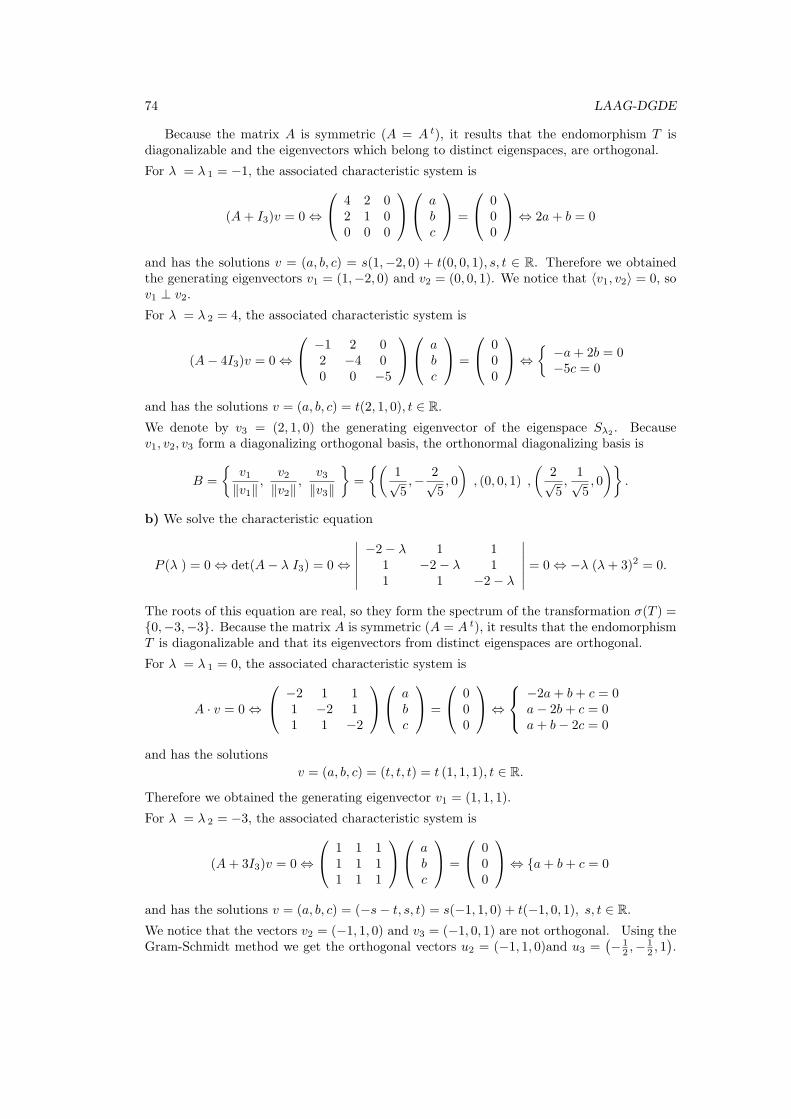
74 LAAG-DGDE
Because the matrix A is symmetric (A = A t), it results that the endomorphism T isdiagonalizable and the eigenvectors which belong to distinct eigenspaces, are orthogonal.
For λ = λ 1 = −1, the associated characteristic system is
(A+ I3)v = 0 ⇔
4 2 02 1 00 0 0
abc
=
000
⇔ 2a+ b = 0
and has the solutions v = (a, b, c) = s(1,−2, 0) + t(0, 0, 1), s, t ∈ R. Therefore we obtainedthe generating eigenvectors v1 = (1,−2, 0) and v2 = (0, 0, 1). We notice that ⟨v1, v2⟩ = 0, sov1 ⊥ v2.
For λ = λ 2 = 4, the associated characteristic system is
(A− 4I3)v = 0 ⇔
−1 2 02 −4 00 0 −5
abc
=
000
⇔{
−a+ 2b = 0−5c = 0
and has the solutions v = (a, b, c) = t(2, 1, 0), t ∈ R.We denote by v3 = (2, 1, 0) the generating eigenvector of the eigenspace Sλ2 . Becausev1, v2, v3 form a diagonalizing orthogonal basis, the orthonormal diagonalizing basis is
B =
{v1∥v1∥
,v2
∥v2∥,
v3∥v3∥
}=
{(1√5,− 2√
5, 0
), (0, 0, 1) ,
(2√5,1√5, 0
)}.
b) We solve the characteristic equation
P (λ ) = 0 ⇔ det(A− λ I3) = 0 ⇔
∣∣∣∣∣∣−2− λ 1 1
1 −2− λ 11 1 −2− λ
∣∣∣∣∣∣ = 0 ⇔ −λ (λ+ 3)2 = 0.
The roots of this equation are real, so they form the spectrum of the transformation σ(T ) ={0,−3,−3}. Because the matrix A is symmetric (A = A t), it results that the endomorphismT is diagonalizable and that its eigenvectors from distinct eigenspaces are orthogonal.
For λ = λ 1 = 0, the associated characteristic system is
A · v = 0 ⇔
−2 1 11 −2 11 1 −2
abc
=
000
⇔
−2a+ b+ c = 0a− 2b+ c = 0a+ b− 2c = 0
and has the solutions
v = (a, b, c) = (t, t, t) = t (1, 1, 1), t ∈ R.
Therefore we obtained the generating eigenvector v1 = (1, 1, 1).
For λ = λ 2 = −3, the associated characteristic system is
(A+ 3I3)v = 0 ⇔
1 1 11 1 11 1 1
abc
=
000
⇔ {a+ b+ c = 0
and has the solutions v = (a, b, c) = (−s− t, s, t) = s(−1, 1, 0) + t(−1, 0, 1), s, t ∈ R.We notice that the vectors v2 = (−1, 1, 0) and v3 = (−1, 0, 1) are not orthogonal. Using theGram-Schmidt method we get the orthogonal vectors u2 = (−1, 1, 0)and u3 =
(− 1
2 ,−12 , 1).
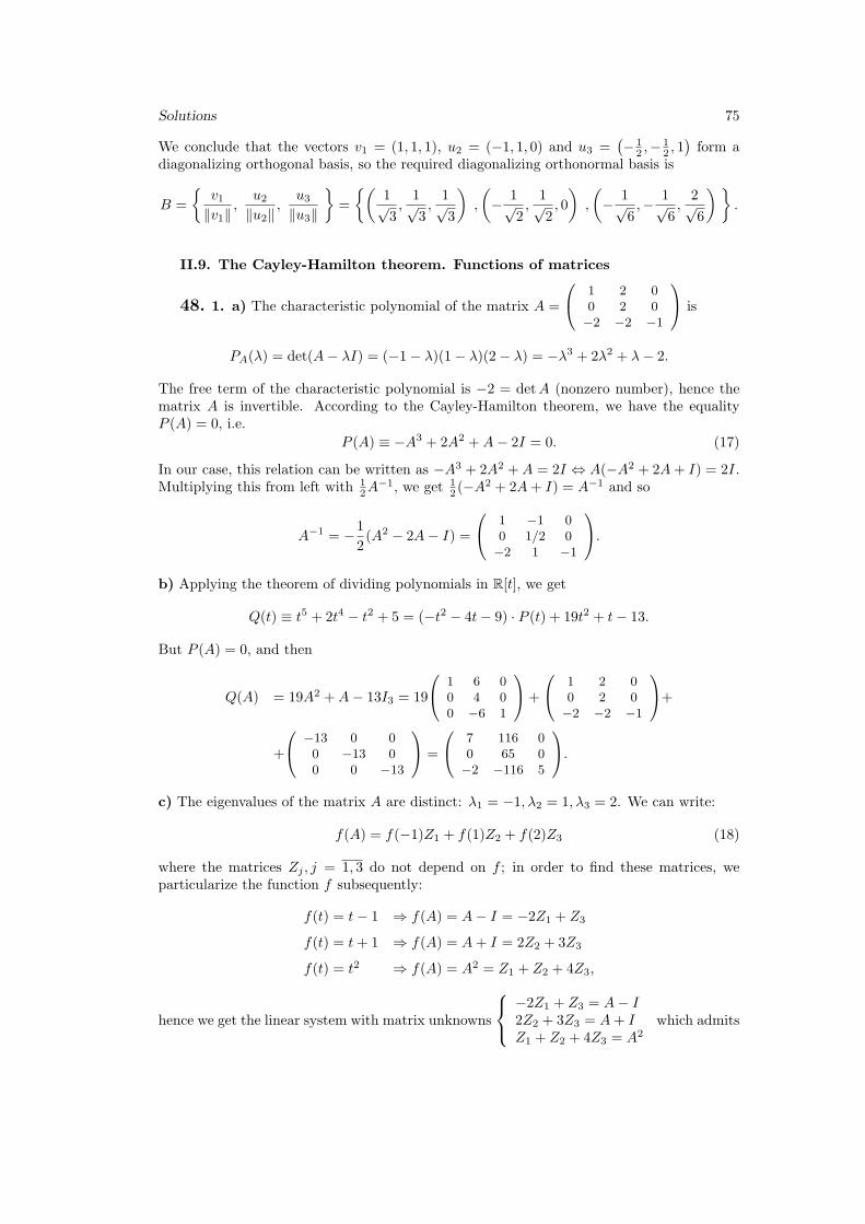
Solutions 75
We conclude that the vectors v1 = (1, 1, 1), u2 = (−1, 1, 0) and u3 =(−1
2 ,−12 , 1)form a
diagonalizing orthogonal basis, so the required diagonalizing orthonormal basis is
B =
{v1
∥v1∥,
u2∥u2∥
,u3∥u3∥
}=
{(1√3,1√3,1√3
),
(− 1√
2,1√2, 0
),
(− 1√
6,− 1√
6,2√6
) }.
II.9. The Cayley-Hamilton theorem. Functions of matrices
48. 1. a) The characteristic polynomial of the matrix A =
1 2 00 2 0−2 −2 −1
is
PA(λ) = det(A− λI) = (−1− λ)(1− λ)(2− λ) = −λ3 + 2λ2 + λ− 2.
The free term of the characteristic polynomial is −2 = detA (nonzero number), hence thematrix A is invertible. According to the Cayley-Hamilton theorem, we have the equalityP (A) = 0, i.e.
P (A) ≡ −A3 + 2A2 +A− 2I = 0. (17)
In our case, this relation can be written as −A3 + 2A2 +A = 2I ⇔ A(−A2 + 2A+ I) = 2I.Multiplying this from left with 1
2A−1, we get 1
2 (−A2 + 2A+ I) = A−1 and so
A−1 = −1
2(A2 − 2A− I) =
1 −1 00 1/2 0−2 1 −1
.b) Applying the theorem of dividing polynomials in R[t], we get
Q(t) ≡ t5 + 2t4 − t2 + 5 = (−t2 − 4t− 9) · P (t) + 19t2 + t− 13.
But P (A) = 0, and then
Q(A) = 19A2 +A− 13I3 = 19
1 6 00 4 00 −6 1
+
1 2 00 2 0−2 −2 −1
+
+
−13 0 00 −13 00 0 −13
=
7 116 00 65 0−2 −116 5
.c) The eigenvalues of the matrix A are distinct: λ1 = −1, λ2 = 1, λ3 = 2. We can write:
f(A) = f(−1)Z1 + f(1)Z2 + f(2)Z3 (18)
where the matrices Zj , j = 1, 3 do not depend on f ; in order to find these matrices, weparticularize the function f subsequently:
f(t) = t− 1 ⇒ f(A) = A− I = −2Z1 + Z3
f(t) = t+ 1 ⇒ f(A) = A+ I = 2Z2 + 3Z3
f(t) = t2 ⇒ f(A) = A2 = Z1 + Z2 + 4Z3,
hence we get the linear system with matrix unknowns
−2Z1 + Z3 = A− I2Z2 + 3Z3 = A+ IZ1 + Z2 + 4Z3 = A2
which admits
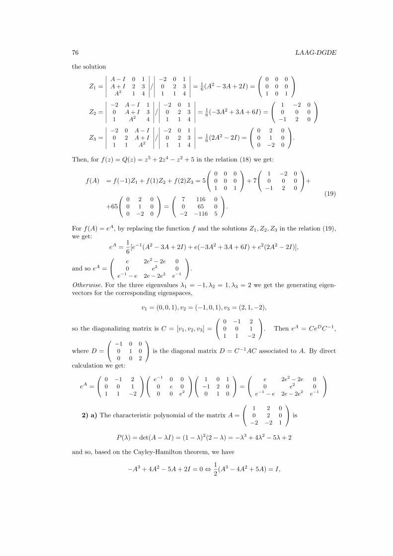
76 LAAG-DGDE
the solution
Z1 =
∣∣∣∣∣∣A− I 0 1A+ I 2 3A2 1 4
∣∣∣∣∣∣/∣∣∣∣∣∣−2 0 10 2 31 1 4
∣∣∣∣∣∣ = 16 (A
2 − 3A+ 2I) =
0 0 00 0 01 0 1
Z2 =
∣∣∣∣∣∣−2 A− I 10 A+ I 31 A2 4
∣∣∣∣∣∣/∣∣∣∣∣∣−2 0 10 2 31 1 4
∣∣∣∣∣∣ = 16 (−3A2 + 3A+ 6I) =
1 −2 00 0 0−1 2 0
Z3 =
∣∣∣∣∣∣−2 0 A− I0 2 A+ I1 1 A2
∣∣∣∣∣∣/∣∣∣∣∣∣−2 0 10 2 31 1 4
∣∣∣∣∣∣ = 16 (2A
2 − 2I) =
0 2 00 1 00 −2 0
.Then, for f(z) = Q(z) = z5 + 2z4 − z2 + 5 in the relation (18) we get:
f(A) = f(−1)Z1 + f(1)Z2 + f(2)Z3 = 5
0 0 00 0 01 0 1
+ 7
1 −2 00 0 0−1 2 0
+
+65
0 2 00 1 00 −2 0
=
7 116 00 65 0−2 −116 5
.(19)
For f(A) = eA, by replacing the function f and the solutions Z1, Z2, Z3 in the relation (19),we get:
eA =1
6[e−1(A2 − 3A+ 2I) + e(−3A2 + 3A+ 6I) + e2(2A2 − 2I)],
and so eA =
e 2e2 − 2e 00 e2 0
e−1 − e 2e− 2e2 e−1
.
Otherwise. For the three eigenvalues λ1 = −1, λ2 = 1, λ3 = 2 we get the generating eigen-vectors for the corresponding eigenspaces,
v1 = (0, 0, 1), v2 = (−1, 0, 1), v3 = (2, 1,−2),
so the diagonalizing matrix is C = [v1, v2, v3] =
0 −1 20 0 11 1 −2
. Then eA = CeDC−1,
where D =
−1 0 00 1 00 0 2
is the diagonal matrix D = C−1AC associated to A. By direct
calculation we get:
eA =
0 −1 20 0 11 1 −2
e−1 0 00 e 00 0 e2
1 0 1−1 2 00 1 0
=
e 2e2 − 2e 00 e2 0
e−1 − e 2e− 2e2 e−1
2) a) The characteristic polynomial of the matrix A =
1 2 00 2 0−2 −2 1
is
P (λ) = det(A− λI) = (1− λ)2(2− λ) = −λ3 + 4λ2 − 5λ+ 2
and so, based on the Cayley-Hamilton theorem, we have
−A3 + 4A2 − 5A+ 2I = 0 ⇔ 1
2(A3 − 4A2 + 5A) = I,
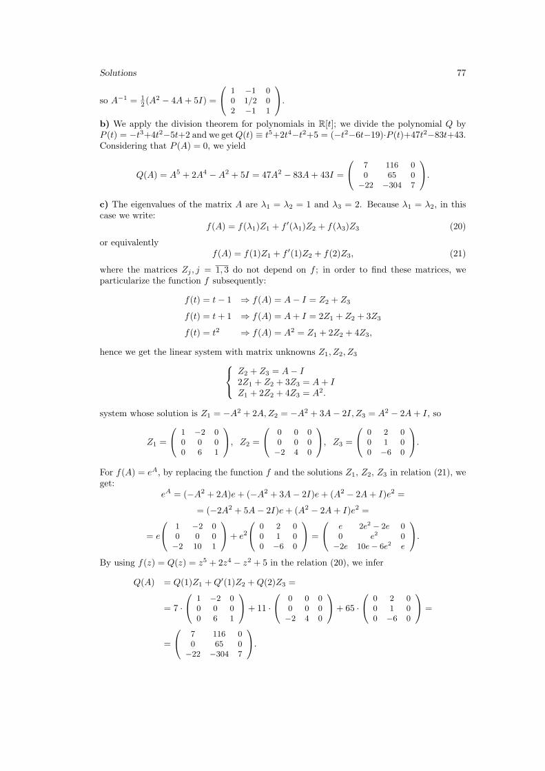
Solutions 77
so A−1 = 12 (A
2 − 4A+ 5I) =
1 −1 00 1/2 02 −1 1
.
b) We apply the division theorem for polynomials in R[t]; we divide the polynomial Q byP (t) = −t3+4t2−5t+2 and we getQ(t) ≡ t5+2t4−t2+5 = (−t2−6t−19)·P (t)+47t2−83t+43.Considering that P (A) = 0, we yield
Q(A) = A5 + 2A4 −A2 + 5I = 47A2 − 83A+ 43I =
7 116 00 65 0
−22 −304 7
.c) The eigenvalues of the matrix A are λ1 = λ2 = 1 and λ3 = 2. Because λ1 = λ2, in thiscase we write:
f(A) = f(λ1)Z1 + f ′(λ1)Z2 + f(λ3)Z3 (20)
or equivalentlyf(A) = f(1)Z1 + f ′(1)Z2 + f(2)Z3, (21)
where the matrices Zj , j = 1, 3 do not depend on f ; in order to find these matrices, weparticularize the function f subsequently:
f(t) = t− 1 ⇒ f(A) = A− I = Z2 + Z3
f(t) = t+ 1 ⇒ f(A) = A+ I = 2Z1 + Z2 + 3Z3
f(t) = t2 ⇒ f(A) = A2 = Z1 + 2Z2 + 4Z3,
hence we get the linear system with matrix unknowns Z1, Z2, Z3 Z2 + Z3 = A− I2Z1 + Z2 + 3Z3 = A+ IZ1 + 2Z2 + 4Z3 = A2.
system whose solution is Z1 = −A2 + 2A,Z2 = −A2 + 3A− 2I, Z3 = A2 − 2A+ I, so
Z1 =
1 −2 00 0 00 6 1
, Z2 =
0 0 00 0 0−2 4 0
, Z3 =
0 2 00 1 00 −6 0
.For f(A) = eA, by replacing the function f and the solutions Z1, Z2, Z3 in relation (21), weget:
eA = (−A2 + 2A)e+ (−A2 + 3A− 2I)e+ (A2 − 2A+ I)e2 =
= (−2A2 + 5A− 2I)e+ (A2 − 2A+ I)e2 =
= e
1 −2 00 0 0−2 10 1
+ e2
0 2 00 1 00 −6 0
=
e 2e2 − 2e 00 e2 0
−2e 10e− 6e2 e
.By using f(z) = Q(z) = z5 + 2z4 − z2 + 5 in the relation (20), we infer
Q(A) = Q(1)Z1 +Q′(1)Z2 +Q(2)Z3 =
= 7 ·
1 −2 00 0 00 6 1
+ 11 ·
0 0 00 0 0−2 4 0
+ 65 ·
0 2 00 1 00 −6 0
=
=
7 116 00 65 0
−22 −304 7
.
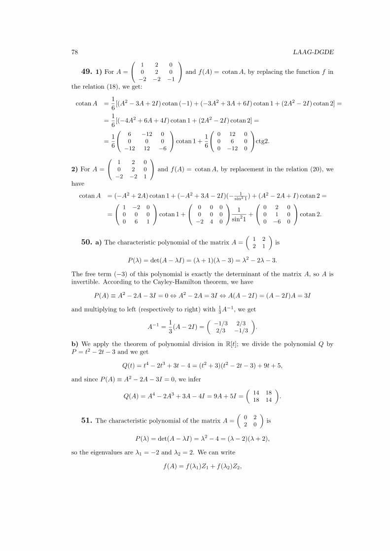
78 LAAG-DGDE
49. 1) For A =
1 2 00 2 0−2 −2 −1
and f(A) = cotanA, by replacing the function f in
the relation (18), we get:
cotanA =1
6[(A2 − 3A+ 2I) cotan (−1) + (−3A2 + 3A+ 6I) cotan 1 + (2A2 − 2I) cotan 2] =
=1
6[(−4A2 + 6A+ 4I) cotan 1 + (2A2 − 2I) cotan 2] =
=1
6
6 −12 00 0 0
−12 12 −6
cotan 1 +1
6
0 12 00 6 00 −12 0
ctg2.
2) For A =
1 2 00 2 0−2 −2 1
and f(A) = cotanA, by replacement in the relation (20), we
have
cotanA = (−A2 + 2A) cotan 1 + (−A2 + 3A− 2I)(− 1sin2 1
) + (A2 − 2A+ I) cotan 2 =
=
1 −2 00 0 00 6 1
cotan 1 +
0 0 00 0 0−2 4 0
1
sin21+
0 2 00 1 00 −6 0
cotan 2.
50. a) The characteristic polynomial of the matrix A =
(1 22 1
)is
P (λ) = det(A− λI) = (λ+ 1)(λ− 3) = λ2 − 2λ− 3.
The free term (−3) of this polynomial is exactly the determinant of the matrix A, so A isinvertible. According to the Cayley-Hamilton theorem, we have
P (A) ≡ A2 − 2A− 3I = 0 ⇔ A2 − 2A = 3I ⇔ A(A− 2I) = (A− 2I)A = 3I
and multiplying to left (respectively to right) with 13A
−1, we get
A−1 =1
3(A− 2I) =
(−1/3 2/32/3 −1/3
).
b) We apply the theorem of polynomial division in R[t]; we divide the polynomial Q byP = t2 − 2t− 3 and we get
Q(t) = t4 − 2t3 + 3t− 4 = (t2 + 3)(t2 − 2t− 3) + 9t+ 5,
and since P (A) ≡ A2 − 2A− 3I = 0, we infer
Q(A) = A4 − 2A3 + 3A− 4I = 9A+ 5I =
(14 1818 14
).
51. The characteristic polynomial of the matrix A =
(0 22 0
)is
P (λ) = det(A− λI) = λ2 − 4 = (λ− 2)(λ+ 2),
so the eigenvalues are λ1 = −2 and λ2 = 2. We can write
f(A) = f(λ1)Z1 + f(λ2)Z2,
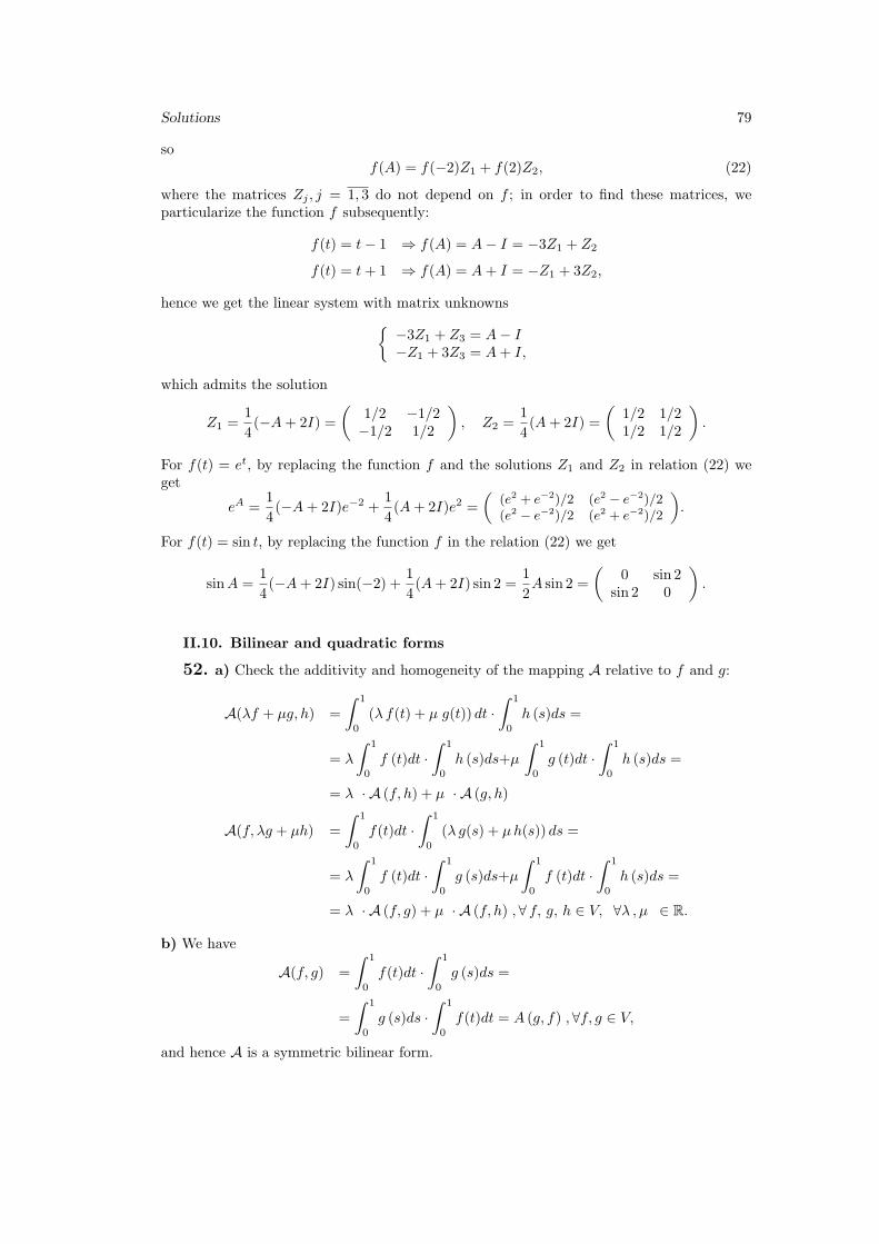
Solutions 79
sof(A) = f(−2)Z1 + f(2)Z2, (22)
where the matrices Zj , j = 1, 3 do not depend on f ; in order to find these matrices, weparticularize the function f subsequently:
f(t) = t− 1 ⇒ f(A) = A− I = −3Z1 + Z2
f(t) = t+ 1 ⇒ f(A) = A+ I = −Z1 + 3Z2,
hence we get the linear system with matrix unknowns{−3Z1 + Z3 = A− I−Z1 + 3Z3 = A+ I,
which admits the solution
Z1 =1
4(−A+ 2I) =
(1/2 −1/2−1/2 1/2
), Z2 =
1
4(A+ 2I) =
(1/2 1/21/2 1/2
).
For f(t) = et, by replacing the function f and the solutions Z1 and Z2 in relation (22) weget
eA =1
4(−A+ 2I)e−2 +
1
4(A+ 2I)e2 =
((e2 + e−2)/2 (e2 − e−2)/2(e2 − e−2)/2 (e2 + e−2)/2
).
For f(t) = sin t, by replacing the function f in the relation (22) we get
sinA =1
4(−A+ 2I) sin(−2) +
1
4(A+ 2I) sin 2 =
1
2A sin 2 =
(0 sin 2
sin 2 0
).
II.10. Bilinear and quadratic forms
52. a) Check the additivity and homogeneity of the mapping A relative to f and g:
A(λf + µg, h) =
∫ 1
0
(λ f(t) + µ g(t)) dt ·∫ 1
0
h (s)ds =
= λ
∫ 1
0
f (t)dt ·∫ 1
0
h (s)ds+µ
∫ 1
0
g (t)dt ·∫ 1
0
h (s)ds =
= λ · A (f, h) + µ · A (g, h)
A(f, λg + µh) =
∫ 1
0
f(t)dt ·∫ 1
0
(λ g(s) + µh(s)) ds =
= λ
∫ 1
0
f (t)dt ·∫ 1
0
g (s)ds+µ
∫ 1
0
f (t)dt ·∫ 1
0
h (s)ds =
= λ · A (f, g) + µ · A (f, h) , ∀ f, g, h ∈ V, ∀λ , µ ∈ R.
b) We have
A(f, g) =
∫ 1
0
f(t)dt ·∫ 1
0
g (s)ds =
=
∫ 1
0
g (s)ds ·∫ 1
0
f(t)dt = A (g, f) , ∀f, g ∈ V,
and hence A is a symmetric bilinear form.
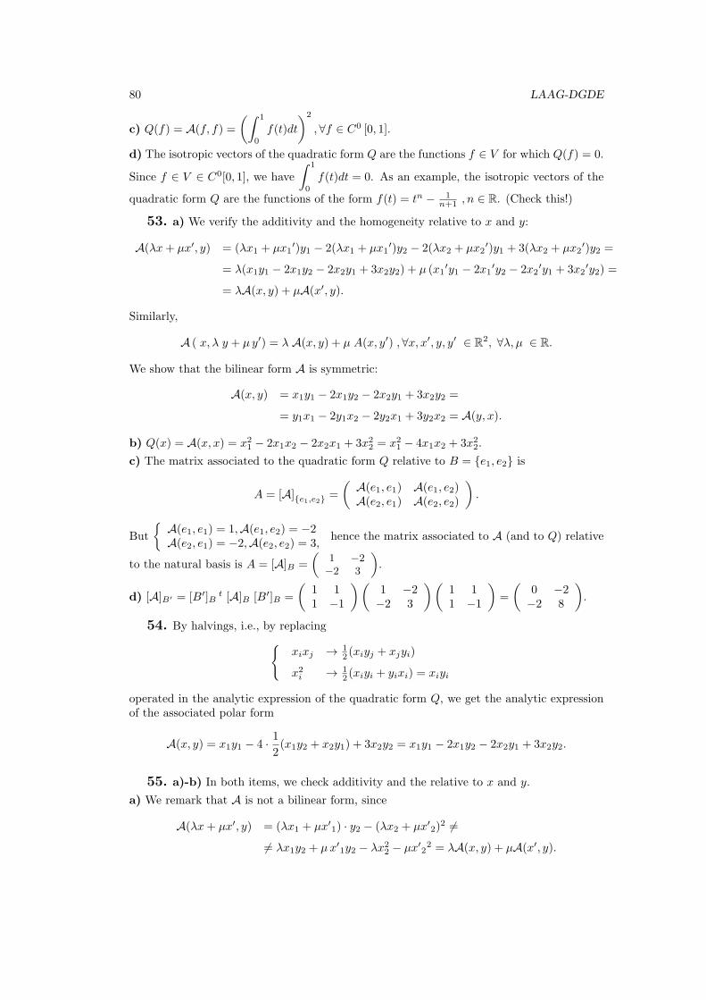
80 LAAG-DGDE
c) Q(f) = A(f, f) =
(∫ 1
0
f(t)dt
)2
,∀f ∈ C0 [0, 1].
d) The isotropic vectors of the quadratic form Q are the functions f ∈ V for which Q(f) = 0.
Since f ∈ V ∈ C0[0, 1], we have
∫ 1
0
f(t)dt = 0. As an example, the isotropic vectors of the
quadratic form Q are the functions of the form f(t) = tn − 1n+1 , n ∈ R. (Check this!)
53. a) We verify the additivity and the homogeneity relative to x and y:
A(λx+ µx′, y) = (λx1 + µx1′)y1 − 2(λx1 + µx1
′)y2 − 2(λx2 + µx2′)y1 + 3(λx2 + µx2
′)y2 =
= λ(x1y1 − 2x1y2 − 2x2y1 + 3x2y2) + µ (x1′y1 − 2x1
′y2 − 2x2′y1 + 3x2
′y2) =
= λA(x, y) + µA(x′, y).
Similarly,
A ( x, λ y + µ y′) = λ A(x, y) + µ A(x, y′) , ∀x, x′, y, y′ ∈ R2, ∀λ, µ ∈ R.
We show that the bilinear form A is symmetric:
A(x, y) = x1y1 − 2x1y2 − 2x2y1 + 3x2y2 =
= y1x1 − 2y1x2 − 2y2x1 + 3y2x2 = A(y, x).
b) Q(x) = A(x, x) = x21 − 2x1x2 − 2x2x1 + 3x22 = x21 − 4x1x2 + 3x22.
c) The matrix associated to the quadratic form Q relative to B = {e1, e2} is
A = [A]{e1,e2} =
(A(e1, e1) A(e1, e2)A(e2, e1) A(e2, e2)
).
But
{A(e1, e1) = 1,A(e1, e2) = −2A(e2, e1) = −2,A(e2, e2) = 3,
hence the matrix associated to A (and to Q) relative
to the natural basis is A = [A]B =
(1 −2−2 3
).
d) [A]B′ = [B′]Bt [A]B [B′]B =
(1 11 −1
)(1 −2−2 3
)(1 11 −1
)=
(0 −2−2 8
).
54. By halvings, i.e., by replacing{xixj → 1
2 (xiyj + xjyi)
x2i → 12 (xiyi + yixi) = xiyi
operated in the analytic expression of the quadratic form Q, we get the analytic expressionof the associated polar form
A(x, y) = x1y1 − 4 · 12(x1y2 + x2y1) + 3x2y2 = x1y1 − 2x1y2 − 2x2y1 + 3x2y2.
55. a)-b) In both items, we check additivity and the relative to x and y.
a) We remark that A is not a bilinear form, since
A(λx+ µx′, y) = (λx1 + µx′1) · y2 − (λx2 + µx′2)2 =
= λx1y2 + µx′1y2 − λx22 − µx′22 = λA(x, y) + µA(x′, y).
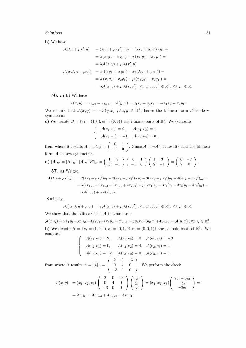
Solutions 81
b) We have
A(λx+ µx′, y) = (λx1 + µx1′) · y2 − (λx2 + µx2
′) · y1 =
= λ(x1y2 − x2y1) + µ (x1′y2 − x2
′y1) =
= λA(x, y) + µA(x′, y)
A(x, λ y + µ y′) = x1(λ y2 + µ y2′)− x2(λ y1 + µ y1
′) =
= λ (x1y2 − x2y1) + µ (x1y2′ − x2y1
′) =
= λA(x, y) + µA(x, y′), ∀x, x′, y, y′ ∈ R2, ∀λ, µ ∈ R.
56. a)-b) We have
A(x, y) = x1y2 − x2y1, A(y, x) = y1x2 − y2x1 = −x1y2 + x2y1.
We remark that A(x, y) = −A(y, x) , ∀x, y ∈ R2, hence the bilinear form A is skew-symmetric.
c) We denote B = {e1 = (1, 0), e2 = (0, 1)} the canonic basis of R2. We compute{A(e1, e1) = 0, A(e1, e2) = 1
A(e2, e1) = −1, A(e2, e2) = 0,
from where it results A = [A]B =
(0 1−1 0
). Since A = −A t, it results that the bilinear
form A is skew-symmetric.
d) [A]B′ = [B′]Bt [A]B [B′]B =
(1 23 −1
)(0 1−1 0
)(1 32 −1
)=
(0 −77 0
).
57. a) We get
A (λx+ µx′, y) = 2(λx1 + µx1′)y1 − 3(λx1 + µx1
′) · y3 − 3(λx3 + µx3′)y1 + 4(λx2 + µx2
′)y2 =
= λ(2x1y1 − 3x1y3 − 3x3y1 + 4x2y2) + µ (2x1′y1 − 3x1
′y3 − 3x3′y1 + 4x2
′y2) =
= λA(x, y) + µA(x′, y).
Similarly,
A ( x, λ y + µ y′) = λ A(x, y) + µA(x, y′) , ∀x, x′, y, y′ ∈ R3, ∀λ, µ ∈ R.
We show that the bilinear form A is symmetric:
A(x, y) = 2x1y1−3x1y3−3x3y1+4x2y2 = 2y1x1−3y1x3−3y3x1+4y2x2 = A(y, x) , ∀x, y ∈ R3.
b) We denote B = {e1 = (1, 0, 0), e2 = (0, 1, 0), e3 = (0, 0, 1)} the canonic basis of R3. Wecompute
A(e1, e1) = 2, A(e1, e2) = 0, A(e1, e3) = −3
A(e2, e1) = 0, A(e2, e2) = 4, A(e2, e3) = 0
A(e3, e1) = −3, A(e3, e2) = 0, A(e3, e3) = 0,
from where it results A = [A]B =
2 0 −30 4 0−3 0 0
. We perform the check
A(x, y) = (x1, x2, x3)
2 0 −30 4 0−3 0 0
y1y2y3
= (x1, x2, x3)
2y1 − 3y34y2−3y1
=
= 2x1y1 − 3x1y3 + 4x2y2 − 3x3y1.
82 LAAG-DGDE
c) The kernel of a bilinear symmetric form is defined by
KerA = {x ∈ V | A(x, y) = 0, ∀ y ∈ V }.
We have
A(x, y) = 0, ∀ y ∈ V ⇔ 2x1y1 − 3x1y3 − 3x3y1 + 4x2y2 = 0, ∀y = (y1, y2, y3) ⇔
⇔ x1 = x2 = x3 = 0 ⇔ x = 0R3 ,
hence KerA = {0}, from where it results dim KerA = 0. The rank of the bilinear form A isequal with the rank of the matrix A. Since detA = −36 = 0, it results rankA = rankA =3. We conclude that it is satisfied the Theorem of dimension:
dim KerA︸ ︷︷ ︸0
+ rankA︸ ︷︷ ︸3
= dimR3︸ ︷︷ ︸3
.
d) Q(x) = A(x, x) = 2x21 − 3x1x3 − 3x3x1 + 4x22 = 2x21 − 6x1x3 + 4x22.
e) Since the matrix A is non-singular, it results that the bilinear form A is non-degenerate.Q admits nonzero isotropic vectors if and only if
Q(x) = 0, x = 0 ⇔ 2x21 − 6x1x3 + 4x22 = 0, (x1, x2, x3) = (0, 0, 0).
Assuming x1 = 0, we get x3 =2x2
1+4x22
6x1= x1
3 +2x2
2
3x1. As an example, for x1 = 1, x2 = 1 it
results x3 = 1; hence for the nonzero vector x = (1, 1, 1) = 0R3 , we have Q(x) = 0.
58. a) We proceed like in problem 52, item a).
b) We compute [A]B′ :
a11 = A(q1, q1) =
(∫ 1
0
(1 + t)dt
)2
=
[(t+ t2
2
)∣∣∣10
]2= 9
4
a12 = A(q1, q2) =
(∫ 1
0
(1 + t)dt
)(∫ 1
0
s2ds
)=(t+ t2
2
)∣∣∣10·(s3
3
)∣∣∣10= 1
2
a13 = A(q1, q3) =
∫ 1
0
(1 + t)dt ·∫ 1
0
1ds =3
2
a21 = a12 = 12 , a22 = A(q2, q2) =
(∫ 1
0
t2dt
)2
= 19
a23 = A(q2, q3) =
∫ 1
0
t2dt ·∫ 1
0
1ds =1
3
a31 = a13 = 32 , a32 = a23 = 1
3 , a33 = A(q3, q3) =
(∫ 1
0
1ds
)2
= 1,
hence A = [A]B′ =
9/4 1/2 3/21/2 1/9 1/33/2 1/3 1
.
c) The kernel of the bilinear form A is:
KerA = {p ∈ V = R2 [x] | A(p, q) = 0,∀ q ∈ R2 [x]} .
We have
A(p, q) = 0, ∀ q ∈ R2 [x] ⇔∫ 1
0
p(t)dt ·∫ 1
0
q(s)ds = 0 , ∀q ∈ R2 [x] ⇔∫ 1
0
p(t)dt = 0. (23)
Solutions 83
We consider the polynomial p ∈ R2 [x] of the form p(x) = ax2 + bx + c. Then the relation(23) can be written∫ 1
0
(at2 + bt+ c)dt = 0 ⇔(at3
3+ b
t2
2+ ct
)∣∣∣∣10
= 0 ⇔
⇔ a3 + b
2 + c = 0 ⇔ c = −a3 − b
2 .
It follows that
p(x) = ax2 + bx−(a
3+b
2
)= a
(x2 − 1
3
)+ b
(x− 1
2
),
hence KerA = L({v1 = x2 − 1
3 , v2 = x− 12
})and since the vectors v1 and v2 are linearly
independent we have B = {v1, v2} a basis in KerA = 0. Hence dim KerA = 2.
The rank of the bilinear form A is equal with the rank of the matrix A, which is equal with1.
It is hence satisfied the Theorem of dimension, dim KerA︸ ︷︷ ︸2
+ rankA︸ ︷︷ ︸1
= dimR2[x]︸ ︷︷ ︸3
.
d) Q(p) = A(p, p) = (∫ 1
0p(t)dt)2.
e) Since the matrix A is singular, it results that the bilinear form A is degenerate. Q admits
non-zero isotropic vectors only if
∫ 1
0
p(t)dt = 0, p = 0 ⇔∫ 1
0
(at2 + bt+ c)dt = 0 ⇔ c =
−a3− b
2.
59. a) By halvings, hence using the substitutions{xixj → 1
2 (xiyj + xjyi)
x2i → 12 (xiyi + yixi) = xiyi
performed in the analytic expression of the quadratic form Q, we get the analytic expressionof the attached polar form:
A(x, y) = x1y1 −1
2(x1y2 +x2y1)+ 2 · 1
2(x2y3 +x3y2) = x1y1 −
1
2x1y2 −
1
2x2y1 +x2y3 +x3y2.
b) Let B = {e1 = (1, 0, 0), e2 = (0, 1, 0), e3 = (0, 0, 1)} be the canonic basis of the space R3.We have:
A(e1, e1) = 1, A(e1, e2) = − 12 , A(e1, e3) = 0
A(e2, e1) = − 12 , A(e2, e2) = 0, A(e2, e3) = 1
A(e3, e1) = 0, A(e3, e2) = 1, A(e3, e3) = 0,
hence A = [A]B =
1 −1/2 0−1/2 0 10 1 0
.
60. a) We have U⊥ ={y = (y1, y2, y3) ∈ R3 | A(v1, y) = 0,A(v2, y) = 0
}. We form the
system of equations {A(v1, y) = 0A(v2, y) = 0
⇔{
2y1 − 3y3 + 4y2 = 0−3y1 + 4y2 = 0,
84 LAAG-DGDE
which has the solutions y = (y1, y2, y3) =(t, 3
4 t,53 t), t ∈ R. We conclude that U⊥ ={
t(1, 34 ,
53
)| t ∈ R
}= L(v3), where v3 =
(1, 34 ,
53
)= 0R3 . Hence a basis in U⊥ is {v3 =
(1; 3/4; 5/3)}.b) From the Grassmann Theorem, we have dim(U∩U⊥) = dimU+dimU⊥−dim(U+U⊥) =2 + 1− 3 = 0, from where it results
U ∩ U⊥ = {0} . (24)
Since v1 , v2 and v3 are three linearly independent vectors in the space R3 of dimension 3, itresults that v1 , v2 and v3 form a basis in R3, hence
R3 = U + U⊥ (25)
From the relations (24) and (25) it results U ⊕ U⊥ = R3.
c) Since U ⊕ U⊥ = R3, the restriction A|U is non-degenerate.
II.11. The canonic expression of quadratic forms
61. Using the relation Q = X t A X, we get the analytic expression of a quadratic formQ:
Q(x) = (x1, x2, x3)
0 1 −21 0 3−2 3 0
x1x2x3
=
= (x2 − 2x3, x1 + 3x3,−2x1 + 3x2)
x1x2x3
=
= x1x2 − 2x1x3 + x1x2 + 3x2x3 − 2x1x3 + 3x2x3 =
= 2x1x2 − 4x1x3 + 6x2x3.
Since the quadratic form Q contains no square, we apply the change of coordinates: x1 = y1 + y2x2 = y1 − y2x3 = y3
⇔
x1x2x3
=
1 1 01 −1 00 0 1
y1y2y3
.We get
Q(y) = 2(y1 + y2)(y1 − y2)− 4(y1 + y2)y3 + 6(y1 − y2)y3 = 2y21 − 2y22 + 2y1y3 − 10y2y3.
Grouping the terms in order to form squares we get:
Q(y) = 2y21 + 2y1y3 − 2y22 − 10y2y3 = 12 (2y1 + y3)
2 − 2y22 − 10y2y3 − 12y
23 =
= 12 (2y1 + y3)
2 + 1−2 (−2y2 − 5y3)
2 +25y232 − y23
2 =
= 12 (2y1 + y3)
2 − 12 (−2y2 − 5y3)
2 + 12y23 ,
from where, examining the groupings of squares, it results the change of coordinates z1 = 2y1 + y3z2 = −2y2 − 5y3z3 = y3
⇔
z1z2z3
=
2 0 10 −2 −50 0 1
y1y2y3
.
Solutions 85
We remark that in these coordinates, the quadratic form as the canonic expression. Inorder to obtain the basis to which these coordinates correspond, we note that the coordinatetransformation inverse is:
y1 = 12z1 −
12z3
y2 = − 12z2 −
52z3
y3 = z3
⇔
y1y2y3
=
1/2 0 −1/20 −1/2 −5/20 0 1
z1z2z3
.Finally, the relation between the initial coordinates (x1, x2, x3) and the final ones (z1, z2, z3)is: x1
x2
x3
=
1 1 01 −1 00 0 1
1/2 0 −1/20 −1/2 −5/20 0 1
z1z2z3
=
1/2 −1/2 −31/2 1/2 20 0 1
z1z2z3
,hence the matrix of passing to the diagonalizing basis is:
[B′] =M =
1/2 −1/2 −31/2 1/2 20 0 1
= C.
The matrix of the quadratic form relative to this basis is the diagonal matrix
[Q]B′ = CtAC =
1/2 0 00 −1/2 00 0 12
.We remark that the signature of the quadratic form Q is (+,−,+) or yet (n+, n−, n0) =(2, 1, 0).
62. Let A = [A] the matrix of the polar form
A(x, y) = x1y1 − 2x1y2 − 2x2y1 + x2y2
(obtained by halvings) associated to the quadratic form Q relative to the natural basis. We
have A =
(1 −2−2 1
). By applying the Jacobi method, by direct calculation we get the
minors
∆0 = 1,∆1 = 1,∆2 =
∣∣∣∣ 1 −2−2 1
∣∣∣∣ = −3
and the vectors of the basis corresponding to:
v1 =1
∆1e1 ≡
(10
)t, v2 =
1
∆2
∣∣∣∣ e1 e21 −2
∣∣∣∣ = −1
3(−2e1 − e2) ≡
(2/31/3
),
hence the matrix of passing to the new basis B′ and the diagonal matrix attached to thequadratic form relative to this basis are respectively
C = [B′]B =
(1 2/30 1/3
), [Q]B′ = CtAC =
(∆0/∆1 0
0 ∆1/∆2
)=
(1 00 −1/3
),
and the analytic expression of the form relative to the new coordinates [x]B′ = (x′1, x′2)t is
Q(x) = x′21 − 13x
′22.
63. The spectrum of the matrix A =
(1 −2−2 1
)associated to the quadratic form Q
is σ(A) = {−1, 3}. For λ1 = −1 we find an associated generating eigenvector, by solving thecharacteristic system
(A− (−1)I)v = 0 ⇒(
2 −2−2 2
)(xy
)=
(00
)⇔{x = ty = t
, t ∈ R.
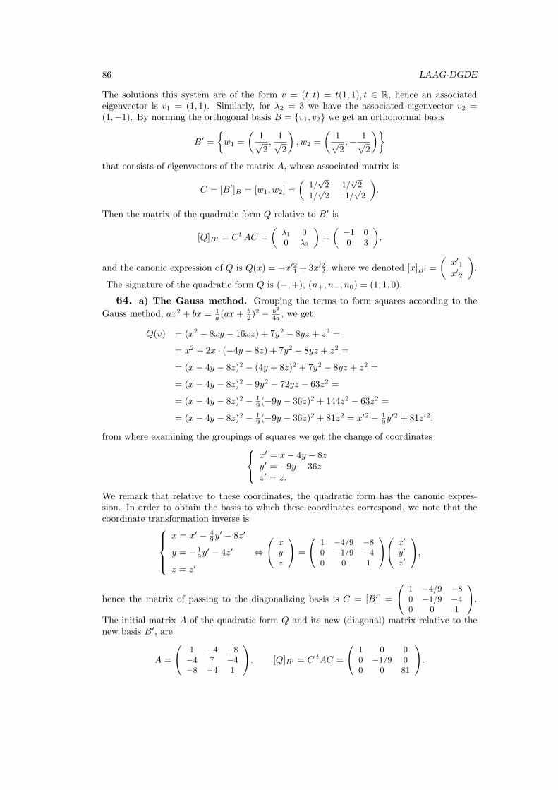
86 LAAG-DGDE
The solutions this system are of the form v = (t, t) = t(1, 1), t ∈ R, hence an associatedeigenvector is v1 = (1, 1). Similarly, for λ2 = 3 we have the associated eigenvector v2 =(1,−1). By norming the orthogonal basis B = {v1, v2} we get an orthonormal basis
B′ =
{w1 =
(1√2,1√2
), w2 =
(1√2,− 1√
2
)}that consists of eigenvectors of the matrix A, whose associated matrix is
C = [B′]B = [w1, w2] =
(1/
√2 1/
√2
1/√2 −1/
√2
).
Then the matrix of the quadratic form Q relative to B′ is
[Q]B′ = CtAC =
(λ1 00 λ2
)=
(−1 00 3
),
and the canonic expression of Q is Q(x) = −x′21 + 3x′22, where we denoted [x]B′ =
(x′1x′2
).
The signature of the quadratic form Q is (−,+), (n+, n−, n0) = (1, 1, 0).
64. a) The Gauss method. Grouping the terms to form squares according to the
Gauss method, ax2 + bx = 1a (ax+ b
2 )2 − b2
4a , we get:
Q(v) = (x2 − 8xy − 16xz) + 7y2 − 8yz + z2 =
= x2 + 2x · (−4y − 8z) + 7y2 − 8yz + z2 =
= (x− 4y − 8z)2 − (4y + 8z)2 + 7y2 − 8yz + z2 =
= (x− 4y − 8z)2 − 9y2 − 72yz − 63z2 =
= (x− 4y − 8z)2 − 19 (−9y − 36z)2 + 144z2 − 63z2 =
= (x− 4y − 8z)2 − 19 (−9y − 36z)2 + 81z2 = x′2 − 1
9y′2 + 81z′2,
from where examining the groupings of squares we get the change of coordinates x′ = x− 4y − 8zy′ = −9y − 36zz′ = z.
We remark that relative to these coordinates, the quadratic form has the canonic expres-sion. In order to obtain the basis to which these coordinates correspond, we note that thecoordinate transformation inverse is
x = x′ − 49y
′ − 8z′
y = − 19y
′ − 4z′
z = z′
⇔
xyz
=
1 −4/9 −80 −1/9 −40 0 1
x′
y′
z′
,
hence the matrix of passing to the diagonalizing basis is C = [B′] =
1 −4/9 −80 −1/9 −40 0 1
.
The initial matrix A of the quadratic form Q and its new (diagonal) matrix relative to thenew basis B′, are
A =
1 −4 −8−4 7 −4−8 −4 1
, [Q]B′ = C tAC =
1 0 00 −1/9 00 0 81
.
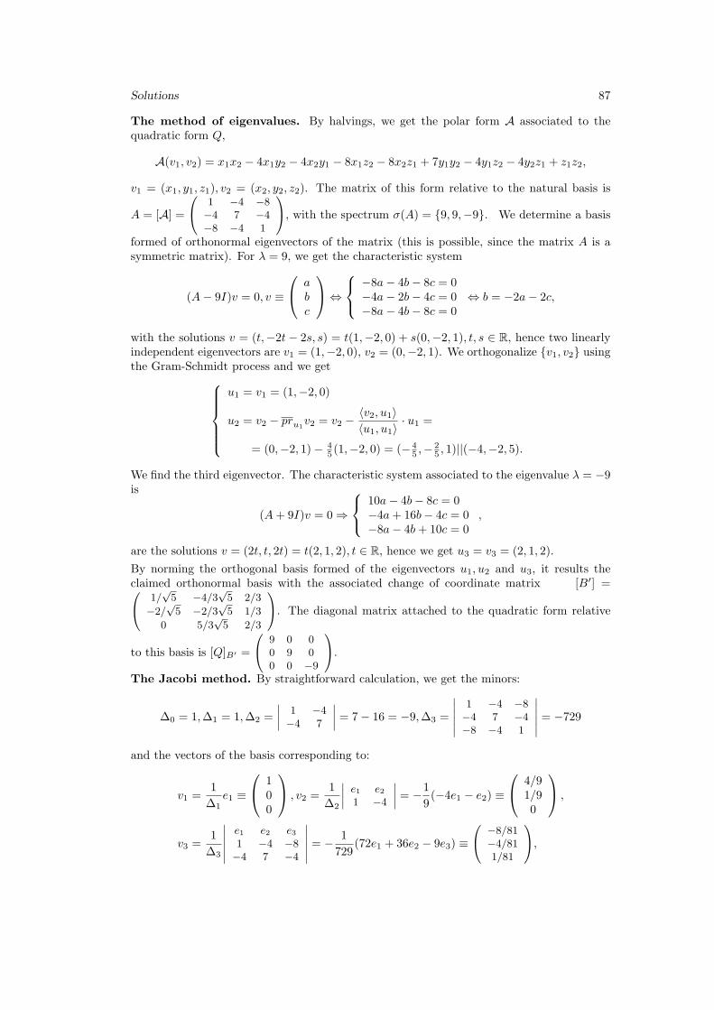
Solutions 87
The method of eigenvalues. By halvings, we get the polar form A associated to thequadratic form Q,
A(v1, v2) = x1x2 − 4x1y2 − 4x2y1 − 8x1z2 − 8x2z1 + 7y1y2 − 4y1z2 − 4y2z1 + z1z2,
v1 = (x1, y1, z1), v2 = (x2, y2, z2). The matrix of this form relative to the natural basis is
A = [A] =
1 −4 −8−4 7 −4−8 −4 1
, with the spectrum σ(A) = {9, 9,−9}. We determine a basis
formed of orthonormal eigenvectors of the matrix (this is possible, since the matrix A is asymmetric matrix). For λ = 9, we get the characteristic system
(A− 9I)v = 0, v ≡
abc
⇔
−8a− 4b− 8c = 0−4a− 2b− 4c = 0−8a− 4b− 8c = 0
⇔ b = −2a− 2c,
with the solutions v = (t,−2t− 2s, s) = t(1,−2, 0) + s(0,−2, 1), t, s ∈ R, hence two linearlyindependent eigenvectors are v1 = (1,−2, 0), v2 = (0,−2, 1). We orthogonalize {v1, v2} usingthe Gram-Schmidt process and we get
u1 = v1 = (1,−2, 0)
u2 = v2 − pru1v2 = v2 −
⟨v2, u1⟩⟨u1, u1⟩
· u1 =
= (0,−2, 1)− 45 (1,−2, 0) = (−4
5 ,−25 , 1)||(−4,−2, 5).
We find the third eigenvector. The characteristic system associated to the eigenvalue λ = −9is
(A+ 9I)v = 0 ⇒
10a− 4b− 8c = 0−4a+ 16b− 4c = 0−8a− 4b+ 10c = 0
,
are the solutions v = (2t, t, 2t) = t(2, 1, 2), t ∈ R, hence we get u3 = v3 = (2, 1, 2).
By norming the orthogonal basis formed of the eigenvectors u1, u2 and u3, it results theclaimed orthonormal basis with the associated change of coordinate matrix [B′] = 1/
√5 −4/3
√5 2/3
−2/√5 −2/3
√5 1/3
0 5/3√5 2/3
. The diagonal matrix attached to the quadratic form relative
to this basis is [Q]B′ =
9 0 00 9 00 0 −9
.
The Jacobi method. By straightforward calculation, we get the minors:
∆0 = 1,∆1 = 1,∆2 =
∣∣∣∣ 1 −4−4 7
∣∣∣∣ = 7− 16 = −9,∆3 =
∣∣∣∣∣∣1 −4 −8−4 7 −4−8 −4 1
∣∣∣∣∣∣ = −729
and the vectors of the basis corresponding to:
v1 =1
∆1e1 ≡
100
, v2 =1
∆2
∣∣∣∣ e1 e21 −4
∣∣∣∣ = −1
9(−4e1 − e2) ≡
4/91/90
,
v3 =1
∆3
∣∣∣∣∣∣e1 e2 e31 −4 −8−4 7 −4
∣∣∣∣∣∣ = − 1
729(72e1 + 36e2 − 9e3) ≡
−8/81−4/811/81
,
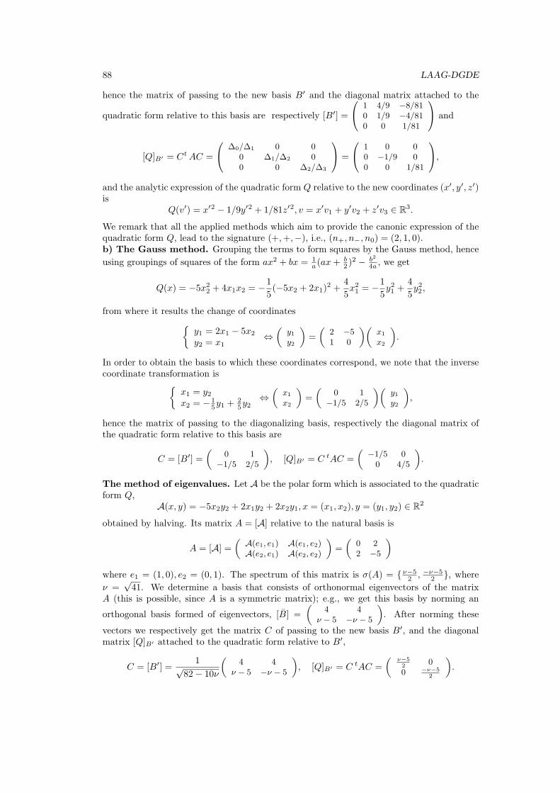
88 LAAG-DGDE
hence the matrix of passing to the new basis B′ and the diagonal matrix attached to the
quadratic form relative to this basis are respectively [B′] =
1 4/9 −8/810 1/9 −4/810 0 1/81
and
[Q]B′ = CtAC =
∆0/∆1 0 00 ∆1/∆2 00 0 ∆2/∆3
=
1 0 00 −1/9 00 0 1/81
,and the analytic expression of the quadratic form Q relative to the new coordinates (x′, y′, z′)is
Q(v′) = x′2 − 1/9y′2 + 1/81z′2, v = x′v1 + y′v2 + z′v3 ∈ R3.
We remark that all the applied methods which aim to provide the canonic expression of thequadratic form Q, lead to the signature (+,+,−), i.e., (n+, n−, n0) = (2, 1, 0).b) The Gauss method. Grouping the terms to form squares by the Gauss method, hence
using groupings of squares of the form ax2 + bx = 1a (ax+ b
2 )2 − b2
4a , we get
Q(x) = −5x22 + 4x1x2 = −1
5(−5x2 + 2x1)
2 +4
5x21 = −1
5y21 +
4
5y22 ,
from where it results the change of coordinates{y1 = 2x1 − 5x2y2 = x1
⇔(
y1y2
)=
(2 −51 0
)(x1
x2
).
In order to obtain the basis to which these coordinates correspond, we note that the inversecoordinate transformation is{
x1 = y2x2 = −1
5y1 +25y2
⇔(
x1
x2
)=
(0 1
−1/5 2/5
)(y1y2
),
hence the matrix of passing to the diagonalizing basis, respectively the diagonal matrix ofthe quadratic form relative to this basis are
C = [B′] =
(0 1
−1/5 2/5
), [Q]B′ = C tAC =
(−1/5 00 4/5
).
The method of eigenvalues. Let A be the polar form which is associated to the quadraticform Q,
A(x, y) = −5x2y2 + 2x1y2 + 2x2y1, x = (x1, x2), y = (y1, y2) ∈ R2
obtained by halving. Its matrix A = [A] relative to the natural basis is
A = [A] =
(A(e1, e1) A(e1, e2)A(e2, e1) A(e2, e2)
)=
(0 22 −5
)where e1 = (1, 0), e2 = (0, 1). The spectrum of this matrix is σ(A) = { ν−5
2 , −ν−52 }, where
ν =√41. We determine a basis that consists of orthonormal eigenvectors of the matrix
A (this is possible, since A is a symmetric matrix); e.g., we get this basis by norming an
orthogonal basis formed of eigenvectors, [B] =
(4 4
ν − 5 −ν − 5
). After norming these
vectors we respectively get the matrix C of passing to the new basis B′, and the diagonalmatrix [Q]B′ attached to the quadratic form relative to B′,
C = [B′] =1√
82− 10ν
(4 4
ν − 5 −ν − 5
), [Q]B′ = C tAC =
(ν−52
00 −ν−5
2
).
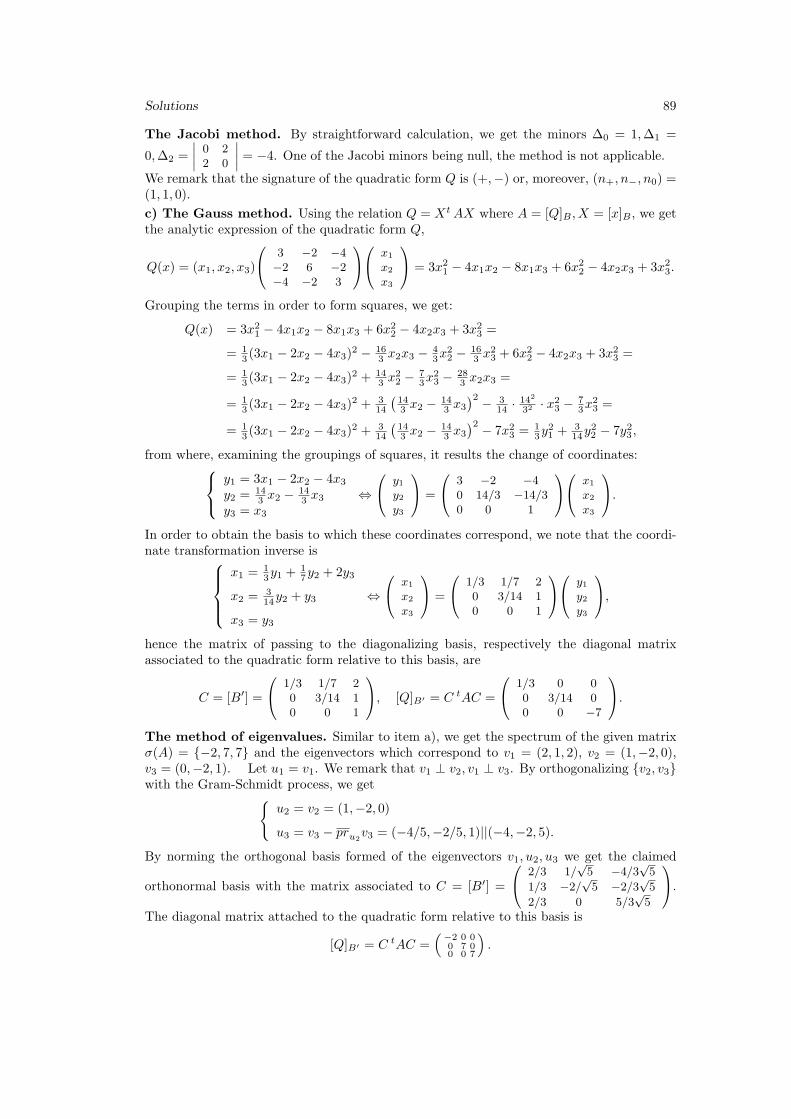
Solutions 89
The Jacobi method. By straightforward calculation, we get the minors ∆0 = 1,∆1 =
0,∆2 =
∣∣∣∣ 0 22 0
∣∣∣∣ = −4. One of the Jacobi minors being null, the method is not applicable.
We remark that the signature of the quadratic form Q is (+,−) or, moreover, (n+, n−, n0) =(1, 1, 0).
c) The Gauss method. Using the relation Q = XtAX where A = [Q]B , X = [x]B , we getthe analytic expression of the quadratic form Q,
Q(x) = (x1, x2, x3)
3 −2 −4−2 6 −2−4 −2 3
x1
x2
x3
= 3x21 − 4x1x2 − 8x1x3 + 6x22 − 4x2x3 + 3x23.
Grouping the terms in order to form squares, we get:
Q(x) = 3x21 − 4x1x2 − 8x1x3 + 6x22 − 4x2x3 + 3x23 =
= 13 (3x1 − 2x2 − 4x3)
2 − 163 x2x3 −
43x
22 − 16
3 x23 + 6x22 − 4x2x3 + 3x23 =
= 13 (3x1 − 2x2 − 4x3)
2 + 143 x
22 − 7
3x23 − 28
3 x2x3 =
= 13 (3x1 − 2x2 − 4x3)
2 + 314
(143 x2 −
143 x3
)2 − 314 · 142
32 · x23 − 73x
23 =
= 13 (3x1 − 2x2 − 4x3)
2 + 314
(143 x2 −
143 x3
)2 − 7x23 = 13y
21 +
314y
22 − 7y23 ,
from where, examining the groupings of squares, it results the change of coordinates: y1 = 3x1 − 2x2 − 4x3y2 = 14
3 x2 −143 x3
y3 = x3
⇔
y1y2y3
=
3 −2 −40 14/3 −14/30 0 1
x1
x2
x3
.In order to obtain the basis to which these coordinates correspond, we note that the coordi-nate transformation inverse is
x1 = 13y1 +
17y2 + 2y3
x2 = 314y2 + y3
x3 = y3
⇔
x1
x2
x3
=
1/3 1/7 20 3/14 10 0 1
y1y2y3
,hence the matrix of passing to the diagonalizing basis, respectively the diagonal matrixassociated to the quadratic form relative to this basis, are
C = [B′] =
1/3 1/7 20 3/14 10 0 1
, [Q]B′ = C tAC =
1/3 0 00 3/14 00 0 −7
.The method of eigenvalues. Similar to item a), we get the spectrum of the given matrixσ(A) = {−2, 7, 7} and the eigenvectors which correspond to v1 = (2, 1, 2), v2 = (1,−2, 0),v3 = (0,−2, 1). Let u1 = v1. We remark that v1 ⊥ v2, v1 ⊥ v3. By orthogonalizing {v2, v3}with the Gram-Schmidt process, we get{
u2 = v2 = (1,−2, 0)
u3 = v3 − pru2v3 = (−4/5,−2/5, 1)||(−4,−2, 5).
By norming the orthogonal basis formed of the eigenvectors v1, u2, u3 we get the claimed
orthonormal basis with the matrix associated to C = [B′] =
2/3 1/√5 −4/3
√5
1/3 −2/√5 −2/3
√5
2/3 0 5/3√5
.
The diagonal matrix attached to the quadratic form relative to this basis is
[Q]B′ = C tAC =(−2 0 0
0 7 00 0 7
).
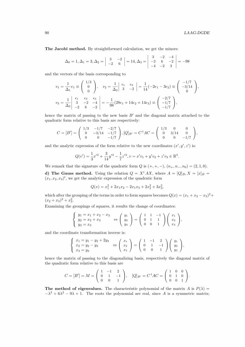
90 LAAG-DGDE
The Jacobi method. By straightforward calculation, we get the minors:
∆0 = 1,∆1 = 3,∆2 =
∣∣∣∣ 3 −2−2 6
∣∣∣∣ = 14,∆3 =
∣∣∣∣∣∣3 −2 −4−2 6 −2−4 −2 3
∣∣∣∣∣∣ = −98
and the vectors of the basis corresponding to
v1 =1
∆1e1 ≡
1/300
, v2 =1
∆2
∣∣∣∣ e1 e23 −2
∣∣∣∣ = 1
14(−2e1 − 3e2) ≡
−1/7−3/14
0
,v3 =
1
∆3
∣∣∣∣∣∣e1 e2 e33 −2 −4−2 6 −2
∣∣∣∣∣∣ = − 1
98(28e1 + 14e2 + 14e3) ≡
−2/7−1/7−1/7
,hence the matrix of passing to the new basis B′ and the diagonal matrix attached to thequadratic form relative to this basis are respectively:
C = [B′] =
1/3 −1/7 −2/70 −3/14 −1/70 0 −1/7
, [Q]B′ = C tAC =
1/3 0 00 3/14 00 0 −1/7
,and the analytic expression of the form relative to the new coordinates (x′, y′, z′) is:
Q(v′) =1
3x′2 +
3
14y′2 − 1
7z′2, v = x′v1 + y′v2 + z′v3 ∈ R3.
We remark that the signature of the quadratic form Q is (+,+,−), (n+, n−, n0) = (2, 1, 0).
d) The Gauss method. Using the relation Q = XtAX, where A = [Q]B , X = [x]B =(x1, x2, x3)
t, we get the analytic expression of the quadratic form
Q(x) = x21 + 2x1x2 − 2x1x3 + 2x22 + 3x23,
which after the grouping of the terms in order to form squares becomesQ(x) = (x1 + x2 − x3)2+
(x2 + x3)2 + x23.
Examining the groupings of squares, it results the change of coordinates: y1 = x1 + x2 − x3y2 = x2 + x3y3 = x3
⇔
y1y2y3
=
1 1 −10 1 10 0 1
x1
x2
x3
,and the coordinate transformation inverse is: x1 = y1 − y2 + 2y3
x2 = y2 − y3x3 = y3
⇔
x1
x2
x3
=
1 −1 20 1 −10 0 1
y1y2y3
,hence the matrix of passing to the diagonalizing basis, respectively the diagonal matrix ofthe quadratic form relative to this basis are
C = [B′] =M =
1 −1 20 1 −10 0 1
, [Q]B′ = C tAC =
1 0 00 1 00 0 1
.The method of eigenvalues. The characteristic polynomial of the matrix A is P (λ) =−λ3 + 6λ2 − 9λ + 1. The roots the polynomial are real, since A is a symmetric matrix;
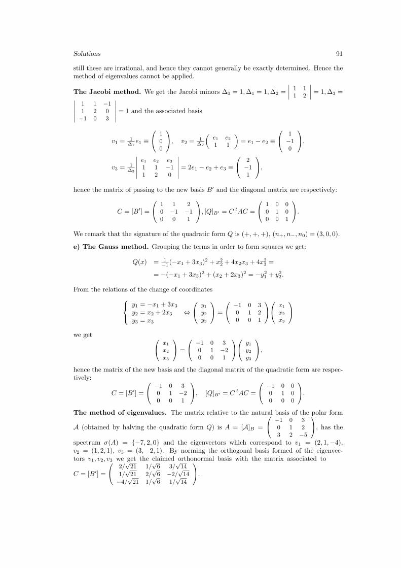
Solutions 91
still these are irrational, and hence they cannot generally be exactly determined. Hence themethod of eigenvalues cannot be applied.
The Jacobi method. We get the Jacobi minors ∆0 = 1,∆1 = 1,∆2 =
∣∣∣∣ 1 11 2
∣∣∣∣ = 1,∆3 =∣∣∣∣∣∣1 1 −11 2 0−1 0 3
∣∣∣∣∣∣ = 1 and the associated basis
v1 = 1∆1e1 ≡
100
, v2 = 1∆2
(e1 e21 1
)= e1 − e2 ≡
1−10
,v3 = 1
∆3
∣∣∣∣∣∣e1 e2 e31 1 −11 2 0
∣∣∣∣∣∣ = 2e1 − e2 + e3 ≡
2−11
,hence the matrix of passing to the new basis B′ and the diagonal matrix are respectively:
C = [B′] =
1 1 20 −1 −10 0 1
, [Q]B′ = C tAC =
1 0 00 1 00 0 1
.We remark that the signature of the quadratic form Q is (+,+,+), (n+, n−, n0) = (3, 0, 0).
e) The Gauss method. Grouping the terms in order to form squares we get:
Q(x) = 1−1 (−x1 + 3x3)
2 + x22 + 4x2x3 + 4x23 =
= −(−x1 + 3x3)2 + (x2 + 2x3)
2 = −y21 + y22 .
From the relations of the change of coordinates y1 = −x1 + 3x3y2 = x2 + 2x3y3 = x3
⇔
y1y2y3
=
−1 0 30 1 20 0 1
x1
x2
x3
we get x1
x2
x3
=
−1 0 30 1 −20 0 1
y1y2y3
,hence the matrix of the new basis and the diagonal matrix of the quadratic form are respec-tively:
C = [B′] =
−1 0 30 1 −20 0 1
, [Q]B′ = C tAC =
−1 0 00 1 00 0 0
.The method of eigenvalues. The matrix relative to the natural basis of the polar form
A (obtained by halving the quadratic form Q) is A = [A]B =
−1 0 30 1 23 2 −5
, has the
spectrum σ(A) = {−7, 2, 0} and the eigenvectors which correspond to v1 = (2, 1,−4),v2 = (1, 2, 1), v3 = (3,−2, 1). By norming the orthogonal basis formed of the eigenvec-tors v1, v2, v3 we get the claimed orthonormal basis with the matrix associated to
C = [B′] =
2/√21 1/
√6 3/
√14
1/√21 2/
√6 −2/
√14
−4/√21 1/
√6 1/
√14
.
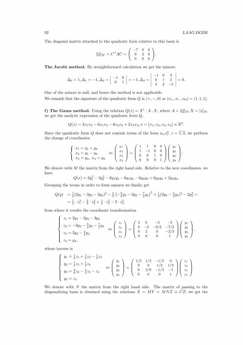
92 LAAG-DGDE
The diagonal matrix attached to the quadratic form relative to this basis is
[Q]B′ = C tAC =
−7 0 00 2 00 0 0
.The Jacobi method. By straightforward calculation we get the minors:
∆0 = 1,∆1 = −1,∆2 =
∣∣∣∣ −1 00 1
∣∣∣∣ = −1,∆3 =
∣∣∣∣∣∣−1 0 30 1 23 2 −5
∣∣∣∣∣∣ = 0.
One of the minors is null, and hence the method is not applicable.
We remark that the signature of the quadratic form Q is (+,−, 0) or (n+, n−, n0) = (1, 1, 1).
f) The Gauss method. Using the relation Q(x) = Xt ·A ·X, where A = [Q]B , X = [x]B ,we get the analytic expression of the quadratic form Q,
Q(x) = 2x1x2 − 6x1x3 − 6x2x4 + 2x3x4, x = (x1, x2, x3, x4) ∈ R4.
Since the quadratic form Q does not contain terms of the form aiix2i , i = 1, 4, we perform
the change of coordinates x1 = y1 + y2x2 = y1 − y2x3 = y3, x4 = y4
⇔
x1
x2
x3
x4
=
1 1 0 01 −1 0 00 0 1 00 0 0 1
y1y2y3y4
;
We denote with M the matrix from the right hand side. Relative to the new coordinates, wehave
Q(x) = 2y21 − 2y22 − 6y1y3 − 6y1y4 − 6y2y3 + 6y2y4 + 2y3y4.
Grouping the terms in order to form squares we finally get
Q(y) = 12 (2y1 − 3y3 − 3y4)
2 − 29
(−9
2y3 − 3y2 − 72y4)2
+ 12 (2y2 −
23y4)
2 − 2y24 =
= 12 · z21 − 2
9 · z22 + 12 · z23 − 2 · z24 ,
from where it results the coordinate transformation
z1 = 2y1 − 3y3 − 3y4
z2 = −3y2 − 92y3 −
72y4
z3 = 2y2 − 23y4
z4 = y4,
⇔
z1z2z3z4
=
2 0 −3 −30 −3 −9/2 −7/20 2 0 −2/30 0 0 1
y1y2y3y4
,
whose inverse is
y1 = 12z1 +
13z2 −
12z3
y2 = 12z3 +
13z4
y3 = 29z2 −
13z3 − z4
y4 = z4
⇔
y1y2y3y4
=
1/2 1/3 −1/2 00 0 1/2 1/30 2/9 −1/3 −10 0 0 1
z1z2z3z4
.
We denote with N the matrix from the right hand side. The matrix of passing to thediagonalizing basis is obtained using the relations X = MY = MNZ ≡ CZ; we get the
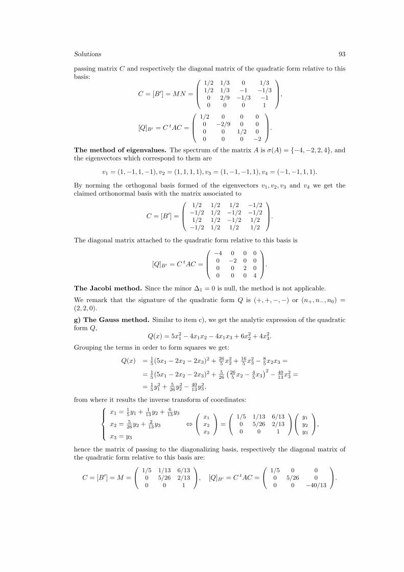
Solutions 93
passing matrix C and respectively the diagonal matrix of the quadratic form relative to thisbasis:
C = [B′] =MN =
1/2 1/3 0 1/31/2 1/3 −1 −1/30 2/9 −1/3 −10 0 0 1
,
[Q]B′ = C tAC =
1/2 0 0 00 −2/9 0 00 0 1/2 00 0 0 −2
.The method of eigenvalues. The spectrum of the matrix A is σ(A) = {−4,−2, 2, 4}, andthe eigenvectors which correspond to them are
v1 = (1,−1, 1,−1), v2 = (1, 1, 1, 1), v3 = (1,−1,−1, 1), v4 = (−1,−1, 1, 1).
By norming the orthogonal basis formed of the eigenvectors v1, v2, v3 and v4 we get theclaimed orthonormal basis with the matrix associated to
C = [B′] =
1/2 1/2 1/2 −1/2−1/2 1/2 −1/2 −1/21/2 1/2 −1/2 1/2−1/2 1/2 1/2 1/2
.The diagonal matrix attached to the quadratic form relative to this basis is
[Q]B′ = C tAC =
−4 0 0 00 −2 0 00 0 2 00 0 0 4
.The Jacobi method. Since the minor ∆1 = 0 is null, the method is not applicable.
We remark that the signature of the quadratic form Q is (+,+,−,−) or (n+, n−, n0) =(2, 2, 0).
g) The Gauss method. Similar to item c), we get the analytic expression of the quadraticform Q,
Q(x) = 5x21 − 4x1x2 − 4x1x3 + 6x22 + 4x23.
Grouping the terms in order to form squares we get:
Q(x) = 15 (5x1 − 2x2 − 2x3)
2 + 265 x
22 +
165 x
23 − 8
5x2x3 =
= 15 (5x1 − 2x2 − 2x3)
2 + 526
(265 x2 −
45x3)2 − 40
13x23 =
= 15y
21 +
526y
22 − 40
13y23 ,
from where it results the inverse transform of coordinates:x1 = 1
5y1 +113y2 +
613y3
x2 = 526y2 +
213y3
x3 = y3
⇔
x1
x2
x3
=
1/5 1/13 6/130 5/26 2/130 0 1
y1y2y3
,hence the matrix of passing to the diagonalizing basis, respectively the diagonal matrix ofthe quadratic form relative to this basis are:
C = [B′] =M =
1/5 1/13 6/130 5/26 2/130 0 1
, [Q]B′ = C tAC =
1/5 0 00 5/26 00 0 −40/13
.
94 LAAG-DGDE
The method of eigenvalues. The spectrum of the matrix A is σ(A) = {2, 5, 8}, and thecorresponding eigenvectors are
v1 = (2, 1, 2), v2 = (1, 2,−2), v3 = (−2, 2, 1).
By norming the orthogonal basis formed of the eigenvectors v1, v2 and v3, we get the claimed
orthonormal basis with the associated matrix [B′] =
2/3 1/3 −2/31/3 2/3 2/32/3 −2/3 1/3
. The diagonal
matrix attached to the quadratic form relative to this basis is [Q]B′ =
2 0 00 5 00 0 8
.
The Jacobi method. By straightforward calculation, we get the minors:
∆0 = 1,∆1 = 5,∆2 =
∣∣∣∣ 5 −2−2 6
∣∣∣∣ = 26,∆3 =
∣∣∣∣∣∣5 −2 −2−2 6 0−2 0 4
∣∣∣∣∣∣ = 80
and the vectors of the basis corresponding to:
v1 =1
∆1e1 ≡
1/500
, v2 =1
∆2
∣∣∣∣ e1 e25 −2
∣∣∣∣ = 1
26(−2e1 − 5e2) ≡
−1/13−5/26
0
,v3 =
1
∆3
∣∣∣∣∣∣e1 e2 e35 −2 −2−2 6 0
∣∣∣∣∣∣ = 1
80(12e1 + 4e2 + 26e3) ≡
3/201/2013/40
,hence the matrix of passing to the new basis B′ and the diagonal matrix attached to thequadratic form relative to this basis are respectively:
C = [B′] =
1/5 −1/13 3/200 −5/26 1/200 0 13/40
, [Q]B′ = C tAC =
1/5 0 00 5/26 00 0 13/40
.We remark that the signature of the quadratic form Q is (+,+,+) or (n+, n−, n0) = (3, 0, 0).
III.1. Free vectors
65. a) We identify the free vectors with the triples of their coordinates relative to thecanonic orthonormal basis
{i, j, k
}, a ≡ (1, 2, µ), b ≡ (1, 1, 2). By straightforward calculation
we get:
a× b =
∣∣∣∣∣∣i j k1 2 µ1 1 2
∣∣∣∣∣∣ = (4− µ)i+ (−2 + µ)j − k.
b) We have ind{a, b}⇔ a × b = 0. In our case a × b = (4 − µ)i + (−2 + µ)j − k = 0 (the
coefficient of k is always non-zero), hence ind{a, b}. But a × b = 0, (a × b)⊥a, (a × b)⊥b,
hence a× b /∈ L(a, b); hence a basis in V3 is given by{a, b, a× b
}.
c) Let O(0, 0, 0) be the origin of the coordinate system and let{i, j, k
}be its basis. Then
the triangle determined by the representatives−→OA and
−−→OB having the same origin O of the
free vectors a and respectively b as adjacent edges has the three vertices O(0, 0, 0), A(1, 2, 2)and B(1, 1, 2). The area of the triangle OAB is given by formula:
A[∆OAB] =1
2
∥∥a× b∥∥ =
1
2∥(1, 2, 2)× (1, 1, 2)∥ =
1
2∥(2, 0,−1)∥ =
1
2
√5.
Solutions 95
Obviously, the area of the parallelogram determined by a and b as adjacent edges is equalwith the double of the area of the triangle OAB, hence equal with
√5.
66. a) We identify the free vectors with the triples of the coordinates relative to canonicorthonormal basis {i, j, k}, a ≡ (1, 1, 1), b ≡ (0, 1, µ), c ≡ (0, 1, 1). We get their joint product:
⟨a, b× c⟩ =
∣∣∣∣∣∣1 1 10 1 µ0 1 1
∣∣∣∣∣∣ = 1− µ.
b) For µ = 1, the three vectors are coplanar (linearly dependent). Since for µ = 1 we have⟨a, b× c
⟩= 0, it results that in this case the three vectors are linearly independent, hence
are non-coplanar. The vectors a, b, c determine in V3 a positive oriented basis if and only if⟨a, b× c
⟩> 0, this being equivalent with µ < 1.
c) The volume of the tetrahedron determined by the vectors a, b, c as adjacent edges isgiven by formula Vt =
16 |⟨a, (b× c)⟩|. Since a triangular prism can be naturally decomposed
into three tetrahedrons of equal volumes, and the parallelepiped-into two prisms of equalvolumes, we have Vpr = 3Vt, Vpp = 2Vpr = 6Vt, hence for µ = 0 we get Vt = 1
6 |1− 0| =16 , Vpr =
12 , Vpp = 1.
67. We have
V[ABCD] =1
6mod
∣∣∣∣∣∣∣∣xA yA zA 1xB yB zB 1xC yC zC 1xD yD zD 1
∣∣∣∣∣∣∣∣ =1
6| − 1| = 1
6.
Otherwise. Since AB = OB − OA ≡ (1, 0, 0) − (0, 0, 0) = (1, 0, 0), AC ≡ (0, 1, 0), andAD ≡ (0, 0, 1), we infer
V[ABCD] =1
6mod (⟨AB,AC ×AD⟩) = 1
6mod
∣∣∣∣∣∣1 0 00 1 00 0 1
∣∣∣∣∣∣ = 1
6.
68. a) We identify the free vectors with the triples of their coordinates relative tothe canonic orthonormal basis
{i, j, k
}, a ≡ (1,−1, 1), b ≡ (1, 2, 3), c ≡ (0, 1, 1). By
straightforward calculation, we get: b× c =
∣∣∣∣∣∣i j k1 2 30 1 1
∣∣∣∣∣∣ = −i− j+ k ≡ (−1,−1, 1) and then,
the double cross product:
a× (b× c) =
∣∣∣∣∣∣i j k1 −1 1−1 −1 1
∣∣∣∣∣∣ = −2j − 2k ≡ (0,−2,−2).
b) By applying the formula a× (b× c) = ⟨a, c⟩ b−⟨a, b⟩c, we have a× (b× c) ≡ 0 · (1, 2, 3)−
2 · (0, 1, 1) = (0,−2,−2) ≡ −2j − 2k.
c) We remark that the double cross product w = a× (b× c) is orthogonal both on a, and alsoon b× c (being the cross product of these vectors). From the relation w = ⟨a, c⟩ b−
⟨a, b⟩c
we remark that the vector w belongs to the subspace L(b, c), being a linear combination ofthe generators of the subspace, hence w is coplanar with b and c.
96 LAAG-DGDE
III.2. The straight line and the plane in space
69. a) The straight line ∆ which passes through the points A(1, 2, 3) and B(4, 2, 1) isgiven by the Cartesian equations:
∆ :x− 1
4− 1=y − 2
2− 2=z − 3
1− 3⇔ x− 1
3=y − 2
0=z − 3
−2.
Making equal the three ratios with t, we get the parametric equations of the straight line,∆ : (x, y, z) = (1 + 3t, 2, 3− 2t), t ∈ R.b) We identify the director vector v with the triple of the coordinates relative to the canonicorthonormal basis
{i, j, k
}, v ≡ (−1, 0, 2). The straight line ∆ determined by the direction
v and item C(2, 6, 1) has the Cartesian equations x−2−1 = y−6
0 = z−12 ; by equalizing the ratios
with t, we get the parametric equations of straight line ∆ : (x, y, z) = (2− t, 6, 1+ 2t), t ∈ R.
70. Solving the system of equations
{2x+ y − 5z = 124x+ 7y − 33z = 1
and by considering as sec-
ondary unknown y = t, we get the parametric equations of straight line ∆ : (x, y, z) =
( 172 + 123 t, t, 1+
523 t), t ∈ R. Extracting t from each equality, we get t =
x− 172
123
= y−01 = z−1
523
,
hence the director vector is v ≡(
123 , 1,
523
)≡ 1
23 i + j + 523 k. Giving values to t ∈ R in the
parametric equations of the straight line ∆, we get points on this straight line. As anexample, for t = 0 and t = 1 we get respectively the points A0(
172 , 0, 1), A1(
39346 , 1,
2823 ) ∈ ∆.
71. We have A,B,C-non-collinear only if ind {AB,AC} ⇔ AB × AC = 0. But AB =
i − 3j, AC = 2i − j and AB × AC =
∣∣∣∣∣∣i j k1 −3 02 −1 0
∣∣∣∣∣∣ = 5k = 0, hence the points A,B and C
are not collinear. The equation of the plane π determined of the points A,B,C is given by:
π :
∣∣∣∣∣∣∣∣x y z 11 −2 1 12 −5 1 13 −3 1 1
∣∣∣∣∣∣∣∣ = 0 ⇔ z = 1.
b) We identify the vector n with the triple of its coordinates relative to the canonic orthonor-mal basis
{i, j, k
}, n ≡ (0, 3, 2). The plane which passes through the point D(1, 5, 0) and
has the normal direction n ≡ (0, 3, 2) is
π : 0(x− 1) + 3(y − 5) + 2(z − 0) = 0 ⇔ 3y + 2z − 15 = 0.
Otherwise. π is part of the parallel pencil of planes of common normal direction n ≡ (0, 3, 2),of the equation πλ : 0x + 3y + 2z + λ = 0, λ ∈ R. The claimed plane contains the pointD(1, 5, 0). The condition D ∈ πλ leads to 3 · 5 + 2 · 0 + λ = 0 ⇒ λ = −15, hence the plane isπ = πλ=−15 : 3y + 2z − 15 = 0.
c) We have the vectors u ≡ (2, 0, 0) and v ≡ (−1, 0, 3). Then the plane π which passesthrough the point E(2, 1, 2) and is parallel with the directions u and v is given by π :∣∣∣∣∣∣x− 2 y − 1 z − 22 0 0−1 0 3
∣∣∣∣∣∣ = 0 ⇔ 6y − 6 = 0 ⇔ y = 1.
d) The normal to the plane unit vector is n = n0/||n0|| ≡(13 ,
23 ,−
23
)≡ (cosα, cosβ, cos γ),
where
α = ^(Ox, n0), β = ^(Oy, n0), γ = ^(Oz, n0)
Solutions 97
are the director angles of the direction given by n0. Applying the Hesse formula, it resultsthe equation of the plane
π : x cosα+ y cosβ + z cos γ − d = 0, (d ≥ 0)
⇔ 13x+ 2
3y +−23 z − 2 = 0 ⇔ x+ 2y − 2z = 6.
Otherwise. The pencil of planes whose normal direction is given by n0 has the Cartesianequation
πλ : 1 · x+ 2 · y − 2 · z + λ = 0 ⇔ λ = −⟨OM, n0
⟩, (26)
where M(x, y, z) ∈ π. We have d (0, πλ) = |λ|∥n0∥ = |λ|
3 . Using the hypothesis, it results|λ|3 = 2 ⇔ λ ∈ {±6}. We want ^
(OM, n0
)to be an acute angle, hence using the relation
(26), we get λ < 0 ⇒ λ = −6, which finally yields
π : x+ 2y − 2z − 6 = 0.
72. We remark that a normal vector of the plane x+ 2y − 3z = 4 is u = (1, 2,−3), andthree points which belong to the plane are A(1, 0,−1),B(2, 1, 0) and C(0, 2, 0). Since, e.g.,the point C does not belong to straight line determined by the points A and B (which hasthe equations x− 1 = y = z + 1) it results that A,B and C are non-collinear (equivalently,check that AB ×AC = 0).
In order to find the parametric equations of the plane, we need a point which belongs tothe plane and two non-collinear vectors u = a1i + b1j + c1k and v = a2i + b2j + c2k whichadmit representatives which are contained in the plane π. Since we know that the oriented
segments−−→AB and
−→AC are contained in the plane, we choose u and v such that
−−→AB ∈ u and−→
AC ∈ v. Then we have :
−−→AB ≡ (a1, b1, c1) = (2− 1, 1− 0, 0− (−1)) = (1, 1, 1),
−→AC ≡ (a2, b2, c2) = (0− 1, 2− 0, 0− (−1)) = (−1, 2, 1).
We conclude that the plane π, which contains the point A(1, 0,−1) = (x0, y0, z0) and whichis parallel to the directions u = i + j + k ≡ (a1, b1, c1) = (1, 1, 1) and v = −i + 2j + k ≡(a2, b2, c2) = (−1, 2, 1), has the parametric equations:
π :
x = x0 + a1s+ a2ty = y0 + b1s+ b2tz = z0 + c1s+ c2t
⇔
x = 1 + s− ty = 0 + s+ 2tz = −1 + s+ t
, s, t ∈ R,
and the Cartesian equation:
π :
∣∣∣∣∣∣x− 1 y − 0 z + 11 1 1−1 2 1
∣∣∣∣∣∣ = 0 ⇔ −1(x− 1)− 2y + 3(z + 1) = 0 ⇔ x+ 2y − 3z = 4.
Homework. Show that {A,B,C} ⊂ π.
73. a) If the algebraic magnitudes of the segments determined by π on the coordinateaxes Ox,Oy and Oz are respectively 1,−3 and 2, it results that the plane π intersects thecoordinate axes at the pointsM1(1, 0, 0),M2(0,−3, 0) andM3(0, 0, 2). We write the equationof the plane by intercepts:
π :x
1+
y
−3+z
2− 1 = 0 ⇔ 6x− 2y + 3z − 6 = 0.
98 LAAG-DGDE
b) We have a point F (1, 2, 3) which belongs to the plane, and a vector parallel to it u ≡(1,−1, 0) (which is given by the director vector of the straight line ∆ : x1 = y−1
−1 = z−10 . We
consider v = FM as the second vector parallel to the plane, where M ∈ ∆ is an arbitrarypoint of the straight line ∆. Let M(0, 1, 1). It follows that v = FM ≡ (0− 1, 1− 2, 1− 3) =(−1,−1,−2). We get:
π :
∣∣∣∣∣∣x− 1 y − 2 z − 31 −1 0−1 −1 −2
∣∣∣∣∣∣ = 0 ⇔ x+ y − z = 0.
Otherwise. We consider ∆ : x = 1 − y = z−10 as being the straight line located at the
intersection of the planes {x = 1− yx = z−1
0
⇔{x+ y − 1 = 0z − 1 = 0,
hence the equation of the reduced pencil of planes which pass through the straight line ∆ is:
(x+ y − 1) + r(z − 1) = 0, r ∈ R.
But π belongs to this pencil and since F (1, 2, 3) ∈ π, we have
(1 + 2− 1) + r(3− 1) = 0 ⇔ 2 + 2r = 0 ⇔ r = −1,
and hence: π : (x+ y − 1)− 1(z − 1) = 0 ⇔ π : x+ y − z = 0.
c) The plane π passes through the point G(2, 0,−1) and has the normal vector n = (1, 0,−3)(the same as the one of the plane π∗ : x− 3z + 1 = 0). We have
π : 1(x− 2) + 0(y − 0) + (−3)(z + 1) = 0 ⇔ x− 3z − 5 = 0.
Otherwise. The reduced pencil of parallel planes which have the same normal direction givenby n = (1, 0,−3) has the equation of the form
πλ : 1 · x+ 0 · y − 3 · z + λ = 0, λ ∈ R.
The plane π belongs to this pencil and contains the point G(2, 0,−1), hence the conditionG ∈ πλ can be written 1 · 2 + 0 · 0− 3 · (−1) + λ = 0 ⇔ λ = −5; hence π : x− 3z − 5 = 0.
III.3. Problems relative to straight lines and planes
74. a) In order to determine the relative position of the straight lines ∆1 and ∆2, wesolve the system determined by the two 2 + 2 equations of the lines:{
x− y = 2, x+ z = 3
2x+ 3z = 4, y = −1.
We remark that the system is incompatible, hence their intersection is the empty set. The
director vectors of the straight lines ∆1 : x1 = y+2
1 = z−3−1 and ∆2 :
x− 12
32
= y+10 = z−1
−1
are respectively v1 = (1, 1,−1) and v2 =(32 , 0,−1
). From calculation it results that
v1 × v2 ≡(−1,− 1
2 ,−32
)= 0R3 , hence the straight lines ∆1 and ∆2 are not parallel. Since
⟨v1, v2⟩ = 52 = 0, it results that the straight lines ∆1 and ∆2 are not perpendicular.
b) The planes π1 : x − 3y = 1 and π2 : 2y + z = 2 have the normal vectors n1 = (1,−3, 0),respectively n2 = (0, 2, 1). Since n1 × n2 = (−3,−1, 2) = 0, the two planes are neither
Solutions 99
parallel, nor confounded, hence their intersection is a straight line ∆∗, whose points satisfythe system of equations: {
x− 3y − 1 = 02y + z − 2 = 0.
We remark that the system is a simple undetermined compatible system, hence π1 and π2intersect by a straight line. Since ⟨n1, n2⟩ = −6 = 0, it results that the two planes are notperpendicular.
75. a) Considering x the secondary unknown in the system
{x− y = 2x+ z = 3
, we get the
solutions:
x = ty = −2 + tz = 3− t
, t ∈ R, from where, extracting t in each of the three relations, it
results the Cartesian equations of straight lines are ∆1 : x−01 = y+2
1 = z−3−1 = t, hence a
director vector of straight lines ∆1 is v1 = i+ j − k ≡ (1, 1,−1).
The Cartesian equations of the straight lines ∆2 are ∆2 :x− 1
232
=y + 1
0=z − 1
−1, hence this
admits as director vector v2 ≡(32 , 0,−1
). We have
cos(∆1,∆2) = cos(v1, v2) =⟨v1, v2⟩∥v1∥ ∥v2∥
=32 + 0 + 1√3 ·√
134
=5√39
39,
and hence (∆1,∆2) = arccos 5√39
39 ∈(0, π2
).
b) We remark that a director vector of the straight lines is ∆ : x−1−1 = y
2 = z+15 is v ≡
(−1, 2, 5), and a normal vector to the plane π : y − z = 1 is n ≡ (0, 1,−1). Let α be theangle between the straight line ∆ and the plane π. We have
sinα =⟨v, n⟩∥v∥ ∥n∥
=−3√30 ·
√2= −
√15
10,
hence α = arcsin −√15
10 = − arcsin√1510 ∈
(−π
2 , 0).
c) We remark that two normal vectors to the planes π1 : x− 3y = 1 and π2 : 2y + z = 2 arerespectively n1 = (1,−3, 0) and n2 = (0, 2, 1). Let θ angle between the two planes. Then:
cos θ = cos(n1, n2) =⟨n1, n2⟩∥n1∥ ∥n2∥
=−6√10 ·
√5= − 6
5√2,
hence θ = π − arccos 65√2∈(π2 , π
).
76. a) We have d(A,B) =√
(−1− 1)2 + (0− 2)2 + (1− 3)2 =√12 = 2
√3.
b) The straight line ∆ : x−1−1 = y
2 = z+15 admits as director vector v ≡ (−1, 2, 5) and contains
the point C(1, 0,−1), which is obtained by canceling the numerators of the ratios. Then
d(A,∆) =∥AC×v∥
∥v∥ . But AC ≡ (0,−2,−4), hence AC × v =
∣∣∣∣∣∣i j k0 −2 −4−1 2 5
∣∣∣∣∣∣ ≡ (2,−4, 2).
It follows that∥∥AC × v
∥∥ =√24 = 2
√6; ∥v∥ =
√30, hence d(A,∆) = 2
√6√
30= 2
√5
5 .
c) The plane π has the equation y − z − 1 = 0. The distance from the point A(1, 2, 3) to π
is d (A, π) = |0·1+1·2+(−1)·3−1|√02+12+(−1)2
= 2√2=
√2.
100 LAAG-DGDE
77. a) The plane π is given by the equation π : y − z = 1, hence a vector normal to theplane is n ≡ (0, 1,−1). The projection of the point A on the plane π is the point B locatedat the intersection of the perpendicular d which passes through A on π. The straight line ∆which passes through A(1, 2, 3) and has the director vector n ≡ (0, 1,−1) has the equations
∆ :x− 1
0=y − 2
1=z − 3
−1.
We find the coordinates of the point B by solving the system:
{B} = π ∩ ∆ :
{x−10 = y−2
1 = z−3−1
y − z = 1⇔
x = 1y + z = 5y − z = 1
⇔
x = 1y = 3z = 2.
It follows that B(1, 3, 2).
b) We remark that the straight line ∆ :x− 1
−1=
y
2=
z + 1
5has the director vector v ≡
(−1, 2, 5). The plane which passes through the point A and is perpendicular on the straightline ∆ has the equation:
π0 : −1(x− 1) + 2(y − 2) + 5(z − 3) = 0 ⇔ x− 2y − 5z + 18 = 0.
The projection A′ of the point A onto the straight line ∆ is found by solving the system:
{A′} = π0 ∩ d :
{x− 2y − 5z + 18 = 0x−1−1 = y
2 = z+15 ,
from where it results A′ ( 15 ,
85 , 3).
c) We find the plane π∗ which passes through ∆ : x−1−1 = y
2 = z+15 and is perpendicular on
π : y − z = 1. This contains the point C(1, 0,−1) ∈ ∆, the director vector v ≡ (−1, 2, 5) ofthe straight line is ∆ and the vector n ≡ (0, 1,−1) normal to π, hence
π∗ :
∣∣∣∣∣∣x− 1 y z + 1−1 2 50 1 −1
∣∣∣∣∣∣ = 0 ⇔ 7x+ y + z = 6.
In this way we find the projection ∆′ = π ∩ π∗:{y − z = 17x+ y + z = 6
78. a) Let A′(x0, y0, z0) be the symmetric of the point A(1, 2, 3) with respect to B.Since B is the middle of the segment [AA′], we have
xB =xA + xA′
2, yB =
yA + yA′
2, zB =
zA + zA′
2,
hence x0+12 = −1, y0+2
2 = 0, z0+32 = 1, from where it results A′(−3,−2,−1).
b) Let A′ be the projection the point A(1, 2, 3) on the straight line ∆, hence A′ is the foot ofthe perpendicular from point A(1, 2, 3) on the straight line ∆ : x−1
−1 = y2 = z+1
5 . The planeπ∗ which passes through A and is perpendicular on ∆ has the equation
π∗ : −1(x− 1) + 2(y − 2) + 5(z − 3) = 0 ⇔ x− 2y − 5z + 18 = 0
We find the coordinates of the point {A′} = π∗ ∩ ∆ by solving the system
A′ :
{x− 2y − 5z + 18 = 0x−1−1 = y
2 = z+15 ,
from where it results A′ ( 15 ,
85 , 3). The symmetric of the point
A relative to the straight line ∆ is the symmetric of A with respect to A′, hence it has thecoordinates A′′ (− 3
5 ,65 , 3).
Solutions 101
c) Let A′′ be the symmetric of A with respect to the plane π. In order to find A′, we writefirst the equations of the straight line ∆∗ which passes through A′ and is perpendicular onπ,
∆∗ :x− 1
0=y − 2
1=z − 3
−1.
The intersection {A′} = ∆∗ ∩ π :
x = 1y + z = 5y − z = 1
leads to prπA = A′(1, 3, 2). We find the
coordinates of A′′: we note that A′ is the middle of AA′′. Hence, from the relations 1+xA′′2 =
1, 2+yA′′2 = 3, 3+zA′′
2 = 2, it results A′′(1, 4, 1).
d) The parametric equations of the straight line ∆ : x−1−1 = y
2 = z+15 = t are ∆ : (x, y, z) =
(1 − t, 2t,−1 + 5t), t ∈ R. For t = 0 and t = 1 we get the points E(1, 0,−1), respectivelyF (0, 2, 4) of the straight lines is ∆. Similarly with item c), we find the symmetric points E′′
and F ′′ of the points E, respectively F , with respect to the plane π : y− z = 1. We remarkthat E ∈ π, hence E′′ = E(1, 0,−1). After calculations, we get F ′′(0, 5, 1). The symmetricof the straight line ∆ with respect to the plane π is the straight line ∆∗ which passes throughE′′(1, 0,−1) and F ′′(0, 5, 1).
∆∗ :x− 1
0− 1=y − 0
5− 0=z + 1
1 + 1⇔ ∆∗ :
x− 1
−1=y
5=z + 1
2.
79. Method I. The Cartesian equations of the two straight lines are: ∆1:x−01 = y+2
1 =z−3−1 (see ex. 75), respectively ∆2 :
x− 12
32
= y+10 = z−1
−1 , hence their director vectors are
v1 ≡ (1, 1,−1), respectively v2 ≡(32 , 0,−1
).
The common perpendicular of the two straight lines has the direction given by the free vector
u = v1 × v2 =
∣∣∣∣∣∣i j k1 1 −132 0 −1
∣∣∣∣∣∣ ≡(−1,−1
2,−3
2
).
Let π∗ the plane which passes through ∆1 (hence contains a point of the straight line ∆1, e.g.,A(0,−2, 3) ∈ ∆1 and the direction of ∆1, given by v1 ≡ (1, 1,−1)) and which contains thedirection of the common perpendicular of the two straight lines, given by n ≡
(−1,− 1
2 ,−32
).
Then:
π∗ :
∣∣∣∣∣∣x− 0 y + 2 z − 31 1 −1−1 −1
2 − 32
∣∣∣∣∣∣ = 0 ⇔ −4x+ 5y + z + 7 = 0.
A point A′ of the common perpendicular is located at the intersection of π∗ with ∆2,
{A′} = ∆2 ∩ π∗ :
{2x−1
3 = y+10 = 1− z
−4x+ 5y + z + 7 = 0⇔
y = −12x+ 3z = 4−4x+ 5y + z = −7
⇔
x = 57
y = −1z = 6
7 ,
hence A′ ( 57 ,−1, 67
).
The common perpendicular ∆⊥ contains the point A′ and has the direction given by n ≡(−1,− 1
2 ,−32
). Then its equations are:
∆⊥ :x− 5
7
−1=y + 1
−12
=z − 6
7
−32
⇔ 7x− 5
−7=
2y + 2
−1=
2z − 12
−21.
Method II. Let v⊥ = v1 × v2 the free vector which gives the direction of the common per-pendicular. The common perpendicular of the straight lines ∆1 and ∆2 is located at the
102 LAAG-DGDE
intersection between the plane π1 = π∗ which passes through ∆1 and is parallel with v⊥ (seeMethod I) and the plane π2 which passes through ∆2 and is parallel with v⊥.
The plane π2 contains a point of the straight line ∆2 (e.g., B( 12 ,−1, 1) ∈ ∆2), the directionof ∆2 given by v2 ≡ ( 32 , 0,−1) and the direction given by the common perpendicular of ∆1
and ∆2, hence of v⊥ ≡ (−1,−12 ,−
32 ).
Then
π2 :
∣∣∣∣∣∣x− 1/2 y + 1 z − 13/2 0 −1−1 −1/2 −3/2
∣∣∣∣∣∣ = 0 ⇔ π2 : −2x+ 13y − 3z + 7 = 0.
We conclude that we have
∆⊥ = π1 ∩ π2 :
{−4x+ 5y + z + 7 = 0
−2x+ 13y − 3z + 17 = 0.
Method III. Using the parametric equations of the two straight lines, we consider the points
C1(t) = (t, t− 2,−t+ 3) ∈ ∆1, t ∈ R, C2(s) = (3/2s+ 1/2,−1,−s+ 1) ∈ ∆2, s ∈ R.
The segment C1(t)C2(s) is included in the common perpendicular ∆1 of the two straightlines only when the vector w = C1(t)C2(s) ≡ ( 3s+1
2 − t,−t+ 1,−s+ t− 2) is orthogonal onthe two director vectors v1 and v2. This condition can be written as{
w⊥v1w⊥v2
⇔{
⟨w, v1⟩ = 0⟨w, v2⟩ = 0
⇔{
−6t+ 5s+ 7 = 0−10t+ 13s+ 11 = 0
⇔{t = 9/7s = 1/7.
The points corresponding to the two values obtained for s and t are respectively
B1 = C1
(9
7
)=
(9
7,−5
7,12
7
)∈ ∆1, B2 = C2
(1
7
)=
(5
7,−1,
6
7
)∈ ∆2.
These are the feet of the common perpendicular ∆⊥, and the straight line B1B2 is exactlythe common perpendicular. We get
∆⊥ :x− 5/7
4/7=y + 1
2/7=z − 6/7
6/7⇔ 7x− 5
4=
7y + 7
2=
7z − 6
6.
We remark that in this way, we can easily compute as well the distance between the twostraight lines. Since B1 ∈ ∆1 and B2 ∈ ∆2 are the feet of the common perpendicular, wehave
d(∆1,∆2) = d(B1, B2) =
√(9
7− 5
7
)2
+
(−5
7+ 1
)2
+
(12
7− 6
7
)2
=2√14
7.
Method IV. We consider two points C1(t) ∈ ∆1 and C2(s) ∈ ∆2 and the function f(s, t) =
||−−−−−−−→C1(t)C2(s)||2, s, t ∈ R. The distance between the two straight lines is given by the minimal
value of the function f when s, t ∈ R. We have
f(s, t) = ( 3s+12 − t)2 + (−t+ 1)2 + (−s+ t− 2)2 =
= 134 · s2 − 3t2 − 5st+ 11
2 · s− 7t+ 214 .
The critical points (s, t) ∈ R2 of the function f (which contains the minimum points) arelocated by solving the system{
∂f∂s = 0∂f∂t = 0
⇔
{132 s− 5t+ 11
2 = 0
6t− 5s− z = 0⇔
{s = 1/7
t = 9/7,
Solutions 103
a unique solution (see the values which were obtained by the method III). Further, in orderto determine the common perpendicular of the straight lines ∆1 and ∆2, we proceed as inMethod III.
80. Two director vectors of the straight lines ∆1:x−01 = y+2
1 = z−3−1 and ∆2 :
x− 12
32
= y+10 = z−1
−1 are v1 ≡ (1, 1,−1) and v2 ≡ (3/2, 0,−1), respectively. Then v1 × v2 ≡(−1,−1/2,−3/2) = 0R3 , which yields that the two lines do not have the same direction. Twopoints on the straight lines are A1(0,−2, 3), and respectively A2
(12 ,−1, 1
). Then:
d(∆1,∆2) =|⟨A1A2, v1 × v2⟩|
||v1 × v2||=
∣∣⟨(12 , 1,−2
),(−1,−1
2 ,−32
)⟩∣∣∥∥(−1,− 12 ,−
32
)∥∥ =
=| 12 · (−1) + 1 ·
(−1
2
)+ (−2) ·
(− 3
2
)|
√14/2
=2√14
7.
81. Two director vectors of the straight lines ∆1 : x−01 = y+2
1 = z−3−1 and ∆2 :
x+ 12
−1 =y−1−1 = z−1
1 are v1 ≡ (1, 1,−1) and v2 ≡ (−1,−1, 1), respectively. Then v1 × v2 ≡ (0, 0, 0) =0R3 , which yields that the two lines have the same direction. Two points on the straight linesare A1(0,−2, 3), and respectively A2
(−1
2 , 1, 1), which yields A1A2 ≡ (−1/2, 3,−2). Then
d(∆1,∆2) = d(A1,∆2) =||v2 ×A1A2||
||v2||=
||(1, 5/2, 7/2)||||(−1,−1, 1)||
=
√78/2√3
=
√13
2.
III.4. Curvilinear coordinates
82. a) We use the formulas
ρ =√x2 + y2
θ =
kπ + arctan y
x , for x = 0
π/2, for x = 0, y > 0
3π/2, for x = 0, y < 0,
(27)
where k = 0, 1, 2, as the point (x, y) is located respectively in quadrants I, II & III, or IV.
We have x = 1, y = −2. Then it results ρ =√x2 + y2 =
√5 and since item is located in the
quadrant IV, θ = 2π + arctan (−2) = 2π − arctan 2.
b) We use the formulas
{x = ρ cos θy = ρ sin θ
, (ρ, θ) ∈ [0,∞)× [0, 2π].
The Cartesian coordinates for ρ = 2 and θ = 3π4 are{
x = 2 cos 3π4 = 2cos
(π − π
4
)= −2cosπ4 = −
√2
y = 2 sin 3π4 = 2 sin
(π − π
4
)= 2 sin π
4 =√2.
83. a) We use the formulas (27). We have x = 1, y = −2, z = −3. Hence ρ =√x2 + y2 =
√5; the projection the point on the plane x0y being located in the quadrant
IV, it results θ = 2π + arctan yx = 2π− arctan 2, and z = −3.
b) We use the formulas
x = ρ cos θy = ρ sin θz = z
, (ρ, θ, z) ∈ [0,∞)× [0, 2π]× R.
104 LAAG-DGDE
We have ρ = 1, θ = 4π3 , z = 2. Then it results:
x = 1 · cos 4π3 = cos
(π + π
3
)= −cosπ3 = −1
2
y = 1 · sin 4π3 = sin
(π + π
3
)= − sinπ3 = −
√32
z = 2.
84. a) We use the formulas
r =√x2 + y2 + z2
φ = arccos(z/r)
θ =
kπ + arctan yx , for x = 0
π/2, for x = 0, y > 03π/2, for x = 0, y < 0.
where k = 0, 1, 2, as the point (x, y, 0) is located respectively in the quadrants I, II &III, or IV of the plane xOy ≡ R2. We have x = 1, y = −2, z = −3, from where we get
r =√x2 + y2 + z2 =
√14 and φ = arccos
(zr
)= arccos
(− 3√
14
)= π − arccos
(3√14
). We
solve the system
{x = r · sinφ · cos θ
y = r · sinφ · sin θ⇔
1 =
√14 ·
√x2+y2√14
· cos θ
−2 =√14 ·
√x2+y2√14
· sin θ⇔
cos θ = 1√5
sin θ = − 2√5⇒ tan θ = −2
and since we are in the quadrant IV, it results θ = 2π+ arctan (−2) = 2π− arctan 2 ∈ [0, 2π).As well, we can write θ = 2π − arcsin 2√
5= 2π − arccos 1√
5.
b) We use the formulas x = r sinφ cos θy = r sinφ sin θz = r cosφ
, (r, φ, θ) ∈ [0,∞)× [0, π]× [0, 2π].
We have r = 1, φ = 2π3 , θ =
5π3 and we get
cosφ = cos(π − π3 ) = − cos π3 = −1
2 , sinφ = sin(π − π3 ) = sin π
3 =√32 ,
cos θ = cos(2π − π3 ) = cos π3 = 1
2 , sin θ = sin(2π − π3 ) = sin(−π
3 ) = − sin π3 = −
√32 ,
hence x = r sinφ cos θ = 1 ·
√32 · 1
2 =√34 ,
y = r sinφ sin θ = 1 ·√32 (−
√32 ) = −3
4 ,
z = r cosφ = 1 · (−12 ) = −1
2 .
Finally, the Cartesian coordinates of the point are (x, y, z) = (√34 ,−
34 ,−
12 ).
III.5. Conics
85. Method 1. The points of the conic satisfy an equation of the form
a11x2 + 2a12xy + a22y
2 + 2a10x+ 2a20y + a00 = 0, (28)
Solutions 105
where the coefficients a11, a12, a22, a10, a20, a00 can be found by solving the system:a11 + 2a12 + a22 + 2a10 + 2a20 + a00 = 0a11 − 2a12 + a22 + 2a10 − 2a20 + a00 = 0a11 − 2a12 + a22 − 2a10 + 2a20 + a00 = 0a11 + 2a12 + a22 − 2a10 − 2a20 + a00 = 014a11 + a10 + a00 = 0
⇔
a11 = −4αa12 = a10 = a20 = 0a22 = 3αa00 = α
, where α ∈ R∗.
We conclude that by replacing the coefficients in (28) and simplifying by α = 0, we get
the equation of the conic Γ : −4x2 + 3y2 + 1 = 0. We remark that δ =
∣∣∣∣ a11 a12
a21 a22
∣∣∣∣ =∣∣∣∣ −4 00 3
∣∣∣∣ = −12 < 0, hence we have a conic of hyperbolic genus. Moreover, since ∆ =∣∣∣∣∣∣a11 a12 a10
a12 a22 a20
a10 a20 a00
∣∣∣∣∣∣ =∣∣∣∣∣∣−4 0 00 3 00 0 1
∣∣∣∣∣∣ = −12 = 0, the conic is non-degenerate, hence it is a
hyperbola.
Method 2. We develop the determinant
Γ :
∣∣∣∣∣∣∣∣∣∣∣∣
x2 xy y2 x y 11 1 1 1 1 11 −1 1 1 −1 11 −1 1 −1 1 11 1 1 −1 −1 114 0 0 1
2 0 1
∣∣∣∣∣∣∣∣∣∣∣∣= 0 ⇔ −x2 + 1
4+
3
4y2 = 0.
We obtain the equation of the claimed conic (hyperbola)
Γ : −4x2 + 3y2 + 1 = 0 ⇔ x2
1/4− y2
1/3= 1.
86. Method I. The claimed conics satisfy equations of the form (28). The conditionA,B,C,D ∈ Γ can be written
a22 + 2a20 + a00 = 0a11 − 2a10 + a00 = 0a22 − 2a20 + a00 = 0a11 + 2a10 + a00 = 0
⇔
a11 = −α, a12 = βa22 = −αa10 = a20 = 0, a00 = α,
where α, β ∈ R are both null. We conclude that the conics which contain the points A,B,Cand D satisfy the equation
Γ : αx2 − 2βxy + αy2 − α = 0, α, β ∈ R, α2 + β2 > 0.
Method II. We apply the formula
Γ : α(AB)(CD) + β(AC)(BD) = 0, α, β ∈ R.
The general equations of the straight lines (AB), (CD), (AC), (BD) are respectively
x− y + 1 = 0, x− y − 1 = 0, x = 0, y = 0.
It follows that the equation of the conic
Γ : α(x− y + 1)(x− y − 1) + γxy = 0 ⇔ αx2 − (2α− γ)xy + αy2 − α = 0,
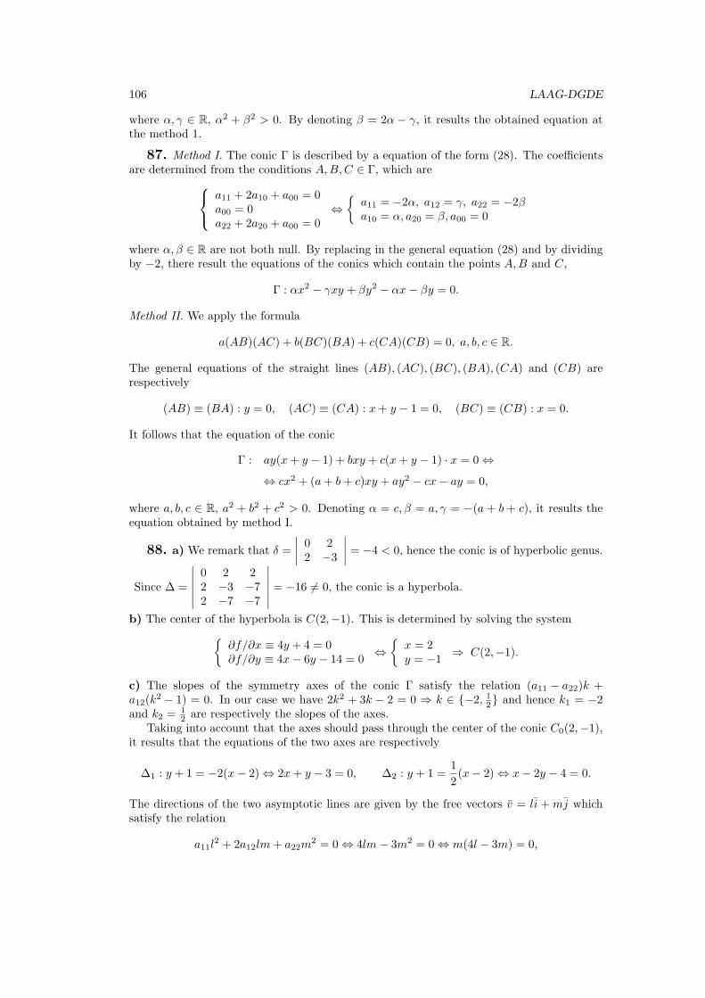
106 LAAG-DGDE
where α, γ ∈ R, α2 + β2 > 0. By denoting β = 2α − γ, it results the obtained equation atthe method 1.
87. Method I. The conic Γ is described by a equation of the form (28). The coefficientsare determined from the conditions A,B,C ∈ Γ, which are a11 + 2a10 + a00 = 0
a00 = 0a22 + 2a20 + a00 = 0
⇔{a11 = −2α, a12 = γ, a22 = −2βa10 = α, a20 = β, a00 = 0
where α, β ∈ R are not both null. By replacing in the general equation (28) and by dividingby −2, there result the equations of the conics which contain the points A,B and C,
Γ : αx2 − γxy + βy2 − αx− βy = 0.
Method II. We apply the formula
a(AB)(AC) + b(BC)(BA) + c(CA)(CB) = 0, a, b, c ∈ R.
The general equations of the straight lines (AB), (AC), (BC), (BA), (CA) and (CB) arerespectively
(AB) ≡ (BA) : y = 0, (AC) ≡ (CA) : x+ y − 1 = 0, (BC) ≡ (CB) : x = 0.
It follows that the equation of the conic
Γ : ay(x+ y − 1) + bxy + c(x+ y − 1) · x = 0 ⇔
⇔ cx2 + (a+ b+ c)xy + ay2 − cx− ay = 0,
where a, b, c ∈ R, a2 + b2 + c2 > 0. Denoting α = c, β = a, γ = −(a + b + c), it results theequation obtained by method I.
88. a) We remark that δ =
∣∣∣∣ 0 22 −3
∣∣∣∣ = −4 < 0, hence the conic is of hyperbolic genus.
Since ∆ =
∣∣∣∣∣∣0 2 22 −3 −72 −7 −7
∣∣∣∣∣∣ = −16 = 0, the conic is a hyperbola.
b) The center of the hyperbola is C(2,−1). This is determined by solving the system{∂f/∂x ≡ 4y + 4 = 0∂f/∂y ≡ 4x− 6y − 14 = 0
⇔{x = 2y = −1
⇒ C(2,−1).
c) The slopes of the symmetry axes of the conic Γ satisfy the relation (a11 − a22)k +a12(k
2 − 1) = 0. In our case we have 2k2 + 3k − 2 = 0 ⇒ k ∈ {−2, 12} and hence k1 = −2and k2 = 1
2 are respectively the slopes of the axes.Taking into account that the axes should pass through the center of the conic C0(2,−1),
it results that the equations of the two axes are respectively
∆1 : y + 1 = −2(x− 2) ⇔ 2x+ y − 3 = 0, ∆2 : y + 1 =1
2(x− 2) ⇔ x− 2y − 4 = 0.
The directions of the two asymptotic lines are given by the free vectors v = li +mj whichsatisfy the relation
a11l2 + 2a12lm+ a22m
2 = 0 ⇔ 4lm− 3m2 = 0 ⇔ m(4l − 3m) = 0,
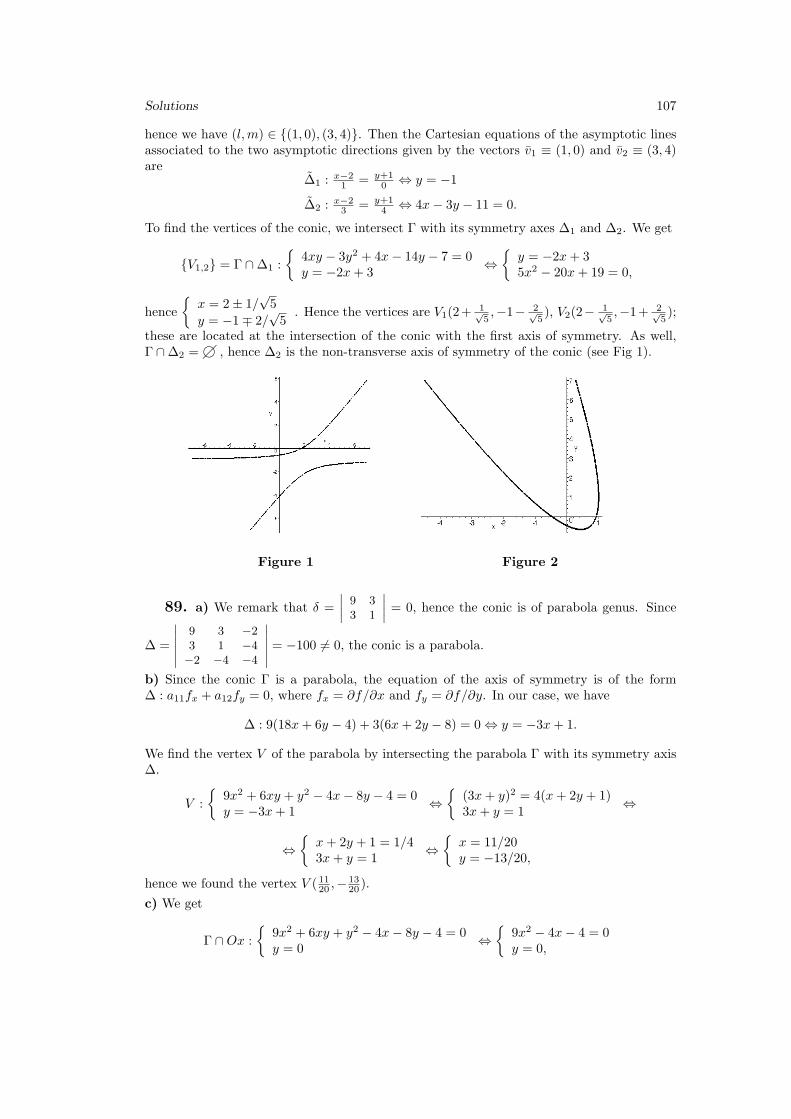
Solutions 107
hence we have (l,m) ∈ {(1, 0), (3, 4)}. Then the Cartesian equations of the asymptotic linesassociated to the two asymptotic directions given by the vectors v1 ≡ (1, 0) and v2 ≡ (3, 4)are
∆1 : x−21 = y+1
0 ⇔ y = −1
∆2 : x−23 = y+1
4 ⇔ 4x− 3y − 11 = 0.
To find the vertices of the conic, we intersect Γ with its symmetry axes ∆1 and ∆2. We get
{V1,2} = Γ ∩∆1 :
{4xy − 3y2 + 4x− 14y − 7 = 0y = −2x+ 3
⇔{y = −2x+ 35x2 − 20x+ 19 = 0,
hence
{x = 2± 1/
√5
y = −1∓ 2/√5
. Hence the vertices are V1(2+1√5,−1− 2√
5), V2(2− 1√
5,−1+ 2√
5);
these are located at the intersection of the conic with the first axis of symmetry. As well,Γ ∩∆2 = g� , hence ∆2 is the non-transverse axis of symmetry of the conic (see Fig 1).
Figure 1 Figure 2
89. a) We remark that δ =
∣∣∣∣ 9 33 1
∣∣∣∣ = 0, hence the conic is of parabola genus. Since
∆ =
∣∣∣∣∣∣9 3 −23 1 −4−2 −4 −4
∣∣∣∣∣∣ = −100 = 0, the conic is a parabola.
b) Since the conic Γ is a parabola, the equation of the axis of symmetry is of the form∆ : a11fx + a12fy = 0, where fx = ∂f/∂x and fy = ∂f/∂y. In our case, we have
∆ : 9(18x+ 6y − 4) + 3(6x+ 2y − 8) = 0 ⇔ y = −3x+ 1.
We find the vertex V of the parabola by intersecting the parabola Γ with its symmetry axis∆.
V :
{9x2 + 6xy + y2 − 4x− 8y − 4 = 0y = −3x+ 1
⇔{
(3x+ y)2 = 4(x+ 2y + 1)3x+ y = 1
⇔
⇔{x+ 2y + 1 = 1/43x+ y = 1
⇔{x = 11/20y = −13/20,
hence we found the vertex V ( 1120 ,−1320 ).
c) We get
Γ ∩Ox :
{9x2 + 6xy + y2 − 4x− 8y − 4 = 0y = 0
⇔{
9x2 − 4x− 4 = 0y = 0,
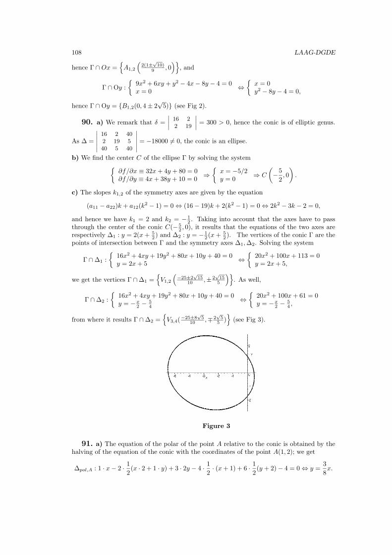
108 LAAG-DGDE
hence Γ ∩Ox ={A1,2
(2(1±
√10)
9 , 0)}
, and
Γ ∩Oy :
{9x2 + 6xy + y2 − 4x− 8y − 4 = 0x = 0
⇔{x = 0y2 − 8y − 4 = 0,
hence Γ ∩Oy = {B1,2(0, 4± 2√5)} (see Fig 2).
90. a) We remark that δ =
∣∣∣∣ 16 22 19
∣∣∣∣ = 300 > 0, hence the conic is of elliptic genus.
As ∆ =
∣∣∣∣∣∣16 2 402 19 540 5 40
∣∣∣∣∣∣ = −18000 = 0, the conic is an ellipse.
b) We find the center C of the ellipse Γ by solving the system{∂f/∂x ≡ 32x+ 4y + 80 = 0∂f/∂y ≡ 4x+ 38y + 10 = 0
⇒{x = −5/2y = 0
⇒ C
(−5
2, 0
).
c) The slopes k1,2 of the symmetry axes are given by the equation
(a11 − a22)k + a12(k2 − 1) = 0 ⇔ (16− 19)k + 2(k2 − 1) = 0 ⇔ 2k2 − 3k − 2 = 0,
and hence we have k1 = 2 and k2 = − 12 . Taking into account that the axes have to pass
through the center of the conic C(−52 , 0), it results that the equations of the two axes are
respectively ∆1 : y = 2(x+ 52 ) and ∆2 : y = − 1
2 (x+ 52 ). The vertices of the conic Γ are the
points of intersection between Γ and the symmetry axes ∆1,∆2. Solving the system
Γ ∩∆1 :
{16x2 + 4xy + 19y2 + 80x+ 10y + 40 = 0y = 2x+ 5
⇔{
20x2 + 100x+ 113 = 0y = 2x+ 5,
we get the vertices Γ ∩∆1 ={V1,2
(−25±2
√15
10 ,± 2√155
)}. As well,
Γ ∩∆2 :
{16x2 + 4xy + 19y2 + 80x+ 10y + 40 = 0y = −x
2 − 54
⇔{
20x2 + 100x+ 61 = 0y = −x
2 − 54 ,
from where it results Γ ∩∆2 ={V3,4(
−25±8√5
10 ,∓2√5
5 )}(see Fig 3).
Figure 3
91. a) The equation of the polar of the point A relative to the conic is obtained by thehalving of the equation of the conic with the coordinates of the point A(1, 2); we get
∆pol,A : 1 · x− 2 · 12(x · 2 + 1 · y) + 3 · 2y − 4 · 1
2· (x+ 1) + 6 · 1
2(y + 2)− 4 = 0 ⇔ y =
3
8x.
Solutions 109
The intersection between the polar straight line ∆ and the conic is given by{x2 − 2xy + 3y2 − 4x+ 6y − 4 = 0y = 3x/8
⇔{
43x2 − 112x− 256 = 0y = 3x/8,
hence we get the points T1,2(56±8
√221
43 , 21±3√221
43 ). Then the two tangent lines which passthrough A have the equations
∆1,2 : y − 2 = (x− 1) · −65± 3√221
13± 8√221
.
b) The diameter of the conic Γ which is conjugate with the direction v = i− 2j ≡ (1,−2) isgiven by the equation
∆conj,v : 1 ·fx+(−2)fy = 0 ⇔ 1 ·(2x− 2y − 4)+(−2)(−2x+ 6y + 6) = 0 ⇔ 3x−7y−8 = 0,
where we denoted fx = ∂f/∂x and fy = ∂f/∂y. If we construct the tangents whose directionsare v ≡ (1,−2) to the conic, then the tangency points {A,B} can be found by solving thesystem
{A,B} = Γ ∩∆conj :
{x2 − 2xy + 3y2 − 4x+ 6y − 4 = 03x− 7y − 8 = 0
⇔{x = (7y + 8)/3y2 + y − 2 = 0
,
from where it results A(−2,−2) and B(5, 1). We conclude that the equations of the tangentstraight lines which have the direction v to the conic are respectively
∆1 : x+21 = y+2
−2 ⇔ 2x+ y + 6 = 0
∆2 : x−51 = y−1
−2 ⇔ 2x+ y − 11 = 0.
c) The tangent line through the point B(1, 1) ∈ Γ to the conic Γ is obtained by halving withthe coordinated the point B,
∆tg,B : 1 · x− (x+ y) + 3 · y − 2(x+ 1) + 3(y + 1)− 4 = 0
or, equivalently, 2x− 5y + 3 = 0.
92. We remark that δ =
∣∣∣∣ 0 22 −3
∣∣∣∣ = −4 < 0, hence we have a conic of hyperbolic
genus. But ∆ =
∣∣∣∣∣∣0 2 22 −3 −72 −7 −7
∣∣∣∣∣∣ = −16 = 0, and hence the conic is a hyperbola. By denoting
k = tanα, the rotation angle α is obtained from the equation
tan 2α =2a12
a11 − a22⇔ 2k
1− k2=
4
0 + 3⇔ 4k2 + 6k − 4 = 0 ⇒ k1,2 ∈
{−2,
1
2
}.
For k = −2, it results
cosα = 1±√1+k2
= 1±√5
sinα = k±√1+k2
= 2±√5
. By choosing cosα = 1√5and sinα = − 2√
5,
we get the rotation matrix C =
(1√5
2√5
− 2√5
1√5
), hence the equations of the rotation of frames
xOy → x′Oy′ become(xy
)= C
(x′
y′
)⇔{x = (x′ + 2y′)/
√5
y = (−2x′ + y′)/√5.

110 LAAG-DGDE
By replacing x, y in the equation of the conic Γ : 4xy − 3y2 + 4x− 14y − 7 = 0, it results itsnew equation, relative to the rotated coordinate system x′Oy′:
Γ :4
5(x′ + 2y′)(−2x′ + y′)− 3
5(−2x′ + y′)2 +
4√5(x′ + 2y′)− 14√
5(−2x′ + y′)− 7 = 0,
which after grouping the squares in x′ and y′, can be written
−4
(x′ − 4√
5
)︸ ︷︷ ︸
x′′
2
+
(y′ − 3√
5
)︸ ︷︷ ︸
y′′
2
+ 4 = 0,
hence we perform the translation X ′ = X ′′ + V ′ given by the relations(x′
y′
)→(x′′
y′′
)=
(x′ − 4√
5
y′ − 3√5
)⇔(x′
y′
)=
(x′′
y′′
)+
(4√53√5
).
Relative to the new coordinates, Γ has a canonic equation (of a hyperbola) Γ : −4x′′2 +
y′′2 + 4 = 0 ⇔ x′′2 − y′′2
4 = 1.
Remark 1. The rotation matrix can be obtained as well by the method of eigenvalues, asfollows. The matrix associated to the quadratic form attached to the conic is:
A =
(a11 a12a21 a22
)=
(0 22 −3
).
We have PA(λ) = det (A−λI) =∣∣∣∣ −λ 2
2 −3− λ
∣∣∣∣ = λ2 + 3λ − 4. The roots of the charac-
teristic equation λ2 + 3λ − 4 = 0 are λ1 = −4 < 0 and λ2 = 1 > 0, hence the conic is ofhyperbolic genus.
For λ = 1, the associated eigenvectors v = (a, b) satisfy the system
(A− I)v = 0 ⇔(
−1 22 −4
)(ab
)=
(00
)⇔{
−a+ 2b = 02a− 4b = 0
,
which admits the solutions v = (2t, t) = t(2, 1), t ∈ R. For t = 1 we get the associatedeigenvector v1 = (2, 1). Similarly, for λ = −4, we get the eigenvector v2 = (1,−2). Bynorming the two vectors we get the orthonormal basis :{
f1 =
(2√5,1√5
), f2 =
(1√5,− 2√
5
)}.
Since det [f1, f2] < 0, by permuting the columns of the matrix and denoting e1 = f2, e2 = f1,it results the matrix C of the rotation:
C = [e1, e2] =
(1/
√5 2/
√5
−2/√5 1/
√5
),
and the equations of the rotation xOy → x′Oy′ become
{x = (x′ + 2y′)/
√5
y = (−2x′ + y′)/√5
. Using the
eigenvalues and the invariants we can anticipate the canonic equation a of the conic. Wehave λ1 = −4, λ2 = 1 and ∆
δ = −16−4 = 4, hence
Γ′′ : λ1x′′2 + λ2y
′′2 +∆
δ= 0 ⇔ −4x′′2 + y′′2 + 4 = 0 ⇔ x′′2 − y′′2
4= 1.
Solutions 111
Remark 2. The coordinates of the center of symmetry of the hyperbola C0(x, y) satisfy thesystem: {
2y + 2 = 02x− 3y − 7 = 0
⇔{x = 2y = −1
hence we can first perform a translation of the coordinate system xOy → x′C0y′, of vector
OC0 ≡ (2,−1)t: (xy
)=
(x′
y′
)+
(2−1
)⇔{x = x′ + 2y = y′ − 1
,
from where it results Γ : 4x′y′ − 3y′2 + 4 = 0. We remark that it is necessary to perform arotation of frame x′C0y
′ → x′′C0y′′ of matrix C, given by the relations: X ′ = CX ′′. The
matrix C can be determined either by applying the formula
tan 2θ =2a12
a11 − a22, C =
(cos θ − sinθsin θ cos θ
), (29)
or using the method of eigenvalues (see Rem. 1). We obtain the reduced equation of theconic (see Fig 1),
Γ : x′′2 − y′′2
4= 1.
93. The invariants of the conic are:
∆ =
∣∣∣∣∣∣9 3 −23 1 −4−2 −4 −4
∣∣∣∣∣∣ = −100 = 0, δ =
∣∣∣∣ 9 33 1
∣∣∣∣ = 0,
hence the conic is a parabola (a conic without center). Since a12 = 0, we perform a rotationwhose angle θ is the solution of the equation
tan θ = −a11a12
⇔ tan θ = −3.
One can choose cos θ = 1√10, sinθ = − 3√
10(an equivalent choice being cos θ = − 1√
10, sin θ =
3√10), hence the rotation matrix is R =
(1/
√10 3/
√10
−3/√10 1/
√10
), and the rotation formulas are:
(xy
)= R
(x′
y′
)⇔
{x = (x′ + 3y′)/
√10
y = (−3x′ + y′)/√10.
The equation of the conic relative to the rotated system x′Oy′ is (after regrouping a squareand grouping the first degree term and the remaining free term):
10
(y′− 1√
10
)2
= −2√10
(x′− 5
2√10
).
Hence the new coordinates of the translated system x′′Oy′′ are given by the relations y′′ =y′ − 1√
10, x′′ = x′− 5
2√10
and the relations that define the translation are
(x′
y′
)=
(x′′
y′′
)+
52√10
1√10
.
The originO′′ is exactly the vertex of the parabola, which has the coordinates (x′′, y′′) = (0, 0)and (x′, y′) = ( 5
2√10, 1√
10). Relative to the frame x′′Oy′′ the conic has the canonic equation
112 LAAG-DGDE
Γ : y′′2 = − 2√10x′′. Remark. The rotation matrix can be obtained as well by the method
of eigenvalues, as follows. The matrix associated to the quadratic form attached to the conic
the conic is A =
(9 33 1
). We have PA(λ) = det(A − λI) =
∣∣∣∣ 9− λ 33 1− λ
∣∣∣∣ = λ2 − 10λ.
The roots of the characteristic equation λ2 − 10λ = 0 are λ1 = 0, λ2 = 10, hence the conic isof parabolic genus. For λ = 0, the associated eigenvectors v = (a, b) satisfy the system
(A− λI)v = 0 ⇔(
9 33 1
)(ab
)=
(00
)⇔{
9a+ 3b = 03a+ b = 0
which are the solutions v = (t,−3t) = t(1,−3), t ∈ R. For t = 1, we get the associatedeigenvector v1 = (1,−3). Similarly, for λ = 10, we get the eigenvector v2 = (3, 1). Bynorming the vectors v1 and v2, we get the orthonormal basis
B′ =
{e1 =
(1√10,− 3√
10
), e2 =
(3√10,
1√10
)},
hence the rotation matrix is: R = [e1, e2] =
(1√10
3√10
− 3√10
1√10
); the passing from the coordinate
system xOy to the new, rotated one x′Oy′ is described by the relations{x = (x′ + 3y′)/
√10
y = (−3x′ + y′)/√10.
By replacing this in the equation of the conic relative to the frame xOy, we get the equationrelative to the new frame:
Γ : 10
(y′ − 1√
10
)2
= −2√10
(x′ − 5
2√10
)The two brackets are the expressions of the new coordinates, respectively y′′ = y′− 1√
10, x′′ =
x′ − 52√10, from where there result the equations of the translation x′Oy′ → x′′Oy′′: x′′ = x′ − 5
2√10
y′′ = y′ − 1√10
⇔(x′
y′
)=
(x′′
y′′
)+
52√10
1√10
,
of vector OO′′ =(
52√10, 1√
10
). Finally, the canonic equation of the conic (relative to the
frame x′′O′′y′′) is Γ : y′′2 = − 2√10x′′ (see Fig 2).
Check. We have ∆ = −100, δ = 0, I = 10 ⇒ p =√
−∆I3 = 1√
10hence the reduced equation
of the conic is of the form y2 = ±2px ⇔ y′′2 = ± 2√10x′′ (we obtain the variant with minus
sign).
94. The invariants of the conic are:
∆ =
∣∣∣∣∣∣16 2 402 19 540 5 40
∣∣∣∣∣∣ = −18.000 = 0, δ =
∣∣∣∣ 16 22 19
∣∣∣∣ = 300 > 0,
hence the conic is an ellipse (a conic with center). Since a12 = 0, we perform a rotation ofangle θ, is determined by applying the formula
tan 2θ =2a12
a11 − a22⇔ 2 tan θ
1− tan 2θ= −4
3;
Solutions 113
it results tan θ ∈{2,−1
2
}. For tan θ = 2, one may choose cos θ = 1√
5, sin θ = 2√
5, hence the
rotation matrix is C =
(1√5
− 2√5
2√5
1√5
), and the rotation formulas are:
(xy
)= C
(x′
y′
)⇔{x = (x′ − 2y′)/
√5
y = (2x′ + y′)/√5.
By replacing x, y in the equation of the conic Γ : 16x2 + 4xy + 19y2 + 80x+ 10y + 40 = 0, itresults its new equation, relative to the rotated system of coordinates x′Oy′ :
Γ : 20x′2 + 15y′2 + 20√5 · x′ − 30
√5 · y′ + 40 = 0 ⇔
⇔ 20
(x′ +
√5
2
)︸ ︷︷ ︸
x′′
2
+ 15(y′ −
√5)
︸ ︷︷ ︸y′′
2
= 60,
hence the new coordinates of the translated system x′′Oy′′ are given by the relations x′′ =
x′ +√52 , y′′ = y′ −
√5, and the relations defining the translation are(
x′
y′
)=
(x′′
y′′
)+
(−√5/2√5
).
We obtain the canonic equation of the ellipse Γ : 20x′′2 + 15y′′2 = 60 ⇔ x′′2
3 + y′′2
4 = 1.
Remark 1. The rotation matrix can be obtained as well by the method of eigenvalues, as fol-
lows. The matrix associated to the quadratic form attached to the conic is A =
(16 22 19
).
We have PA(λ) =
∣∣∣∣ 16− λ 22 19− λ
∣∣∣∣ = λ2 − 35λ+300. The roots of the characteristic equa-
tion λ2 − 35λ + 300 = 0 are λ1 = 15 and λ2 = 20, and the orthonormal eigenvectors are
B′ =
{e1 =
(− 2√
5,1√5
), e2 =
(1√5,2√5
)}.
Since det [e1, e2] < 0, by permuting the columns of the matrix, it results the rotation ma-
trix R: R = [e2, e1] =
(1/
√5 −2/
√5
2/√5 1/
√5
), and the equations of the rotation xOy → x′Oy′
become
{x = (x′ − 2y′)/
√5
y = (2x′ + y′)/√5
. Considering the eigenvalues and the invariants we can an-
ticipate the canonic equation of the conic. We have λ1 = 15,λ2 = 20, ∆δ = −60, hence
Γ′′ : λ1x′′2 + λ2y
′′2 +∆
δ= 0 ⇔ 15x′′2 + 20y′′2 − 60 = 0 ⇔ x′′2
4+y′′2
3= 1.
Remark 2. The coordinates of the center of symmetry of the ellipse C0(x, y) satisfy thesystem {
8x+ y + 20 = 02x+ 19y + 5 = 0
⇔{x = − 5
2y = 0
,
hence we can first perform a translation of the coordinate system xOy → x′C0y′, of vector
OC ≡(−5
2 , 0)t, described by the relations:(
xy
)=
(x′
y′
)+
(−5/20
)⇔{x = x′ − 5/2y = y′.
114 LAAG-DGDE
Relative to the new system of coordinates, the equation of the conic is: Γ : 16x′2 + 4x′y′ +19y′2 − 60 = 0. The presence of the term x′y′ in the equation shows that a rotation offrame is needed, x′C0y
′ → x′′C0y′′ of matrix C: X ′ = CX ′′. One can find the matrix C
either by applying the formula tan 2θ =2a12
a11 − a22, C =
(cos θ − sinθsin θ cos θ
), or using the
method of eigenvalues (see Rem. 1 and solving by the method in which rotation proceeds
the translation). Finally, we get Γ : x′′2
3 + y′′2
4 = 1 (see Fig 3).
III.6. Quadrics
95. a) We remark that by grouping the squares, the equation of the sphere Σ can bewritten as
Σ : (x+ 1)2 + (y − 3)2 + (z + 2)2 = 4 ⇔ [x− (−1)]2 + (y − 3)2 + [z − (−2)]2 = 4.
It follows that the center sphere, the point C(−1, 3,−2) and the radius sphere r = 2.
b) The distance from the center C(−1, 3,−2) of sphere to the plane π is
d = d(C, π) =| − 4 + 3− 6 + 13|√
42 + 12 + 32=
6√26
< 2,
hence the plane π is secant to the sphere.
c) By denoting with C ′ the center of the circle Γ obtained by cutting the sphere Σ with theplane π, considering an arbitrary point A of the circle Γ and denoting with r′ its radius, byapplying the Pythagorean Theorem in triangle CC ′A, it results the radius of the sectional
circle r′ =√r2 − d2 =
√3413 . The center C ′ of the circle is located at the intersection of the
plane π with the straight line which passes through C and which is perpendicular on π. Wehave
4x+ y + 3z + 13 = 0
x+ 1
4=y − 3
1=z + 2
3
⇔
x = −25/13y = 36/13z = −35/13
hence we obtain the center C ′(−2513 ,
3613 ,−
3513 ).
96. I. a) For the quadric Σ1, we get g (x, y, z) = x2−y2+z2−2xy−2yz−2zx. The matrix
associated to the quadratic form is: A =
1 −1 −1−1 −1 −1−1 −1 1
, hence σ(A) = {1,−2, 2}. The
invariants of the quadric are:
∆ =
∣∣∣∣∣∣∣∣1 −1 −1 −5/2−1 −1 −1 0−1 −1 1 0
−5/2 0 0 −1
∣∣∣∣∣∣∣∣ =33
2, δ = detA =
∣∣∣∣∣∣1 −1 −1−1 −1 −1−1 −1 1
∣∣∣∣∣∣ = −4
J =
∣∣∣∣ 1 −1−1 −1
∣∣∣∣+ ∣∣∣∣ 1 −1−1 1
∣∣∣∣+ ∣∣∣∣ −1 −1−1 1
∣∣∣∣ = −2 + 0− 2 = −4,
I = Tr A = 1− 1 + 1 = 1.
We conclude that the quadric is non-degenerate (∆ = 0) and admits center of symmetry(since δ = 0).
b) The center of symmetry of the quadric is solution of the system: gx = 0gy = 0gz = 0
⇔
2x− 2y − 2z = 5−2y − 2x− 2z = 02z − 2y − 2x = 0
⇔
x = 5/4y = −5/4z = 0,
⇒ Cs (5/4,−5/4, 0) .
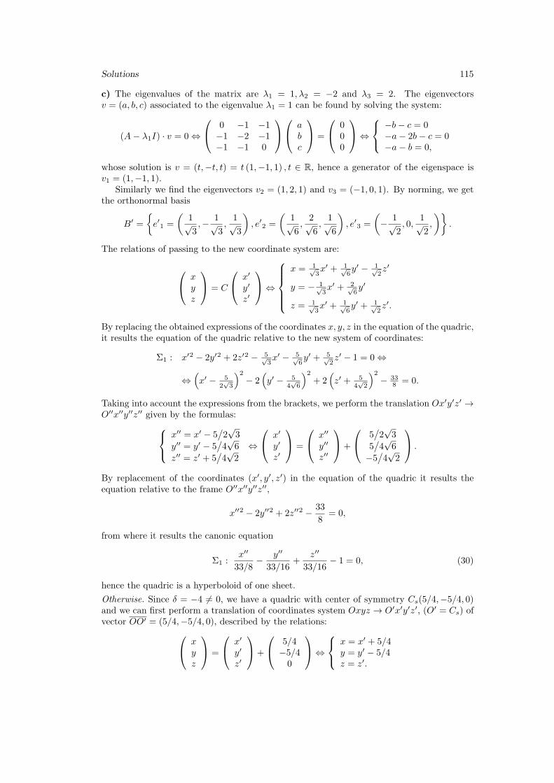
Solutions 115
c) The eigenvalues of the matrix are λ1 = 1, λ2 = −2 and λ3 = 2. The eigenvectorsv = (a, b, c) associated to the eigenvalue λ1 = 1 can be found by solving the system:
(A− λ1I) · v = 0 ⇔
0 −1 −1−1 −2 −1−1 −1 0
abc
=
000
⇔
−b− c = 0−a− 2b− c = 0−a− b = 0,
whose solution is v = (t,−t, t) = t (1,−1, 1) , t ∈ R, hence a generator of the eigenspace isv1 = (1,−1, 1).
Similarly we find the eigenvectors v2 = (1, 2, 1) and v3 = (−1, 0, 1). By norming, we getthe orthonormal basis
B′ =
{e′1 =
(1√3,− 1√
3,1√3
), e′2 =
(1√6,2√6,1√6
), e′3 =
(− 1√
2, 0,
1√2,
)}.
The relations of passing to the new coordinate system are:
xyz
= C
x′
y′
z′
⇔
x = 1√
3x′ + 1√
6y′ − 1√
2z′
y = − 1√3x′ + 2√
6y′
z = 1√3x′ + 1√
6y′ + 1√
2z′.
By replacing the obtained expressions of the coordinates x, y, z in the equation of the quadric,it results the equation of the quadric relative to the new system of coordinates:
Σ1 : x′2 − 2y′2 + 2z′2 − 5√3x′ − 5√
6y′ + 5√
2z′ − 1 = 0 ⇔
⇔(x′ − 5
2√3
)2− 2
(y′ − 5
4√6
)2+ 2
(z′ + 5
4√2
)2− 33
8 = 0.
Taking into account the expressions from the brackets, we perform the translation Ox′y′z′ →O′′x′′y′′z′′ given by the formulas:
x′′ = x′ − 5/2√3
y′′ = y′ − 5/4√6
z′′ = z′ + 5/4√2
⇔
x′
y′
z′
=
x′′
y′′
z′′
+
5/2√3
5/4√6
−5/4√2
.
By replacement of the coordinates (x′, y′, z′) in the equation of the quadric it results theequation relative to the frame O′′x′′y′′z′′,
x′′2 − 2y′′2 + 2z′′2 − 33
8= 0,
from where it results the canonic equation
Σ1 :x′′
33/8− y′′
33/16+
z′′
33/16− 1 = 0, (30)
hence the quadric is a hyperboloid of one sheet.
Otherwise. Since δ = −4 = 0, we have a quadric with center of symmetry Cs(5/4,−5/4, 0)and we can first perform a translation of coordinates system Oxyz → O′x′y′z′, (O′ = Cs) ofvector OO′ = (5/4,−5/4, 0), described by the relations: x
yz
=
x′
y′
z′
+
5/4−5/40
⇔
x = x′ + 5/4y = y′ − 5/4z = z′.
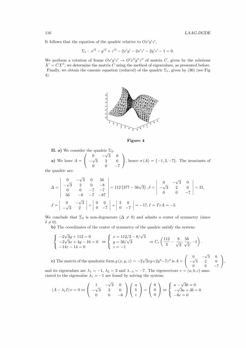
116 LAAG-DGDE
It follows that the equation of the quadric relative to Ox′y′z′,
Σ1 : x′2 − y′2 + z′2 − 2x′y′ − 2x′z′ − 2y′z′ − 1 = 0.
We perform a rotation of frame Ox′y′z′ → O′x′′y′′z′′ of matrix C, given by the relationsX ′ = CX ′′; we determine the matrix C using the method of eigenvalues, as presented before.Finally, we obtain the canonic equation (reduced) of the quadric Σ1, given by (30) (see Fig4).
Figure 4
II. a) We consider the quadric Σ2.
a) We have A =
0 −√3 0
−√3 2 0
0 0 −7
, hence σ (A) = {−1, 3,−7}. The invariants of
the quadric are:
∆ =
∣∣∣∣∣∣∣∣0 −
√3 0 56
−√3 2 0 −8
0 0 −7 −756 −8 −7 −87
∣∣∣∣∣∣∣∣ = 112(377− 56
√3), δ =
∣∣∣∣∣∣0 −
√3 0
−√3 2 0
0 0 −7
∣∣∣∣∣∣ = 21,
J =
∣∣∣∣ 0 −√3
−√3 2
∣∣∣∣+ ∣∣∣∣ 0 00 −7
∣∣∣∣+ ∣∣∣∣ 2 00 −7
∣∣∣∣ = −17, I = TrA = −5.
We conclude that Σ2 is non-degenerate (∆ = 0) and admits a center of symmetry (sinceδ = 0).
b) The coordinates of the center of symmetry of the quadric satisfy the system: −2√3y + 112 = 0
−2√3x+ 4y − 16 = 0
−14z − 14 = 0
⇔
x = 112/3− 8/√3
y = 56/√3
z = −1
⇒ Cs
(112
3− 8√
3,56√3,−1
).
c) The matrix of the quadratic form g (x, y, z) = −2√3xy+2y2−7z2 isA =
0 −√3 0
−√3 2 0
0 0 −7
,
and its eigenvalues are λ1 = −1, λ2 = 3 and λ−3 = −7. The eigenvectors v = (a, b, c) asso-ciated to the eigenvalue λ1 = −1 are found by solving the system:
(A− λ1I) v = 0 ⇔
1 −√3 0
−√3 3 0
0 0 −6
abc
=
000
⇔
a−√3b = 0
−√3a+ 3b = 0
−6c = 0
Solutions 117
whose solutions are v = t(√
3, 1, 0), t ∈ R. For t = 1 we get the generator v1 = (
√3, 1, 0).
Similarly, we find the eigenvectors v2 = (1,−√3, 0) and v3 = (0, 0, 1). By norming, we get
the orthonormal basis
B′ =
{e′1 =
(√3
2,1
2, 0
), e′2 =
(1
2,−
√3
2, 0
), e′3 = (0, 0, 1)
},
whose associated matrix relative to the old basis is:
C0 = [e′1, e′2, e
′3] =
√3/2 1/2 0
1/2 −√3/2 0
0 0 1
.
Since detC0 < 0, we get the rotation matrix C by interchanging the first two columns,
C =
1/2√3/2 0
−√3/2 1/2 00 0 1
.
The relations of passing to the new coordinate system are: xyz
= C
x′
y′
z′
⇔
x = 1
2x′ +
√32 y
′
y = −√32 x
′ + 12y
′
z = z′.
The equation of the quadric relative to the new rotated coordinate system Ox′y′z′ is:
Σ2 : 3x′2 − y′2 − 7z′2 + 8(7 +
√3)x′ + 8
(7√3− 1
)y′ − 14z′ − 87 = 0 ⇔
⇔ 3
(x′ +
4(7+√3)
3
)2
−(y′ − 4
(7√3− 1
))2 − 7 (z′ + 1)2+ a = 0,
where a =16(377−56
√3)
3 > 0. Taking into account the expressions from the brackets, weperform the translation Ox′y′z′ → O′′x′′y′′z′′ given by the formulas:
x′′ = x′ +4(7+
√3)
3
y′′ = y′ − 4(7√3− 1
)z′′ = z′ + 1
⇔
x′
y′
z′
=
x′′
y′′
z′′
+
−4(7 +
√3)/
3
4(7 +
√3)
−1
.
By replacing (x′, y′, z′) in the equation of the quadric, it results a hyperboloid of one sheet,
whose reduced equation is (see Fig 5) −x′′2
a/3 + y′′2
a + z′′2
a/7 = 1.
III. a) We have A =
1 −3 1−3 1 −11 −1 5
, hence σ(A) = {−2, 3, 6}. The invariants of the
quadric are:
∆ =
∣∣∣∣∣∣∣∣1 −3 1 −2−3 1 −1 41 −1 5 −6−2 4 −6 14
∣∣∣∣∣∣∣∣ = −216, δ =
∣∣∣∣∣∣1 −3 1−3 1 −11 −1 5
∣∣∣∣∣∣ = −36
J =
∣∣∣∣ 1 −3−3 1
∣∣∣∣+ ∣∣∣∣ 1 11 5
∣∣∣∣+ ∣∣∣∣ 1 −1−1 5
∣∣∣∣ = −8 + 4 + 4 = 0, I = TrA = 1 + 1 + 5 = 7.
118 LAAG-DGDE
Figure 5
b) The coordinates of the center of symmetry of the quadric are the solutions the system: 2x− 6y + 2z − 4 = 02y − 6x− 2z + 8 = 010z + 2x− 2y − 12 = 0
⇔
x− 3y + z = 2−3x+ y − z = −4x− y + 5z = 6
⇒ Cs(1, 0, 1).
c) The matrix associated to the quadratic form
g(x, y, z) = x2 + y2 + 5z2 − 6xy + 2xz − 2yz
of the quadric is A =
1 −3 1−3 1 −11 −1 5
. A basis that consists of eigenvectors associated to
the eigenvalues λ1 = −2, λ2 = 3 and λ3 = 6 is {v1 = (1, 1, 0), v2 = (−1, 1, 1), v3 = (1,−1, 2)}.By norming, we get the orthonormal basis
B′ =
{e′1 =
(1√2,1√2, 0
), e′2 =
(− 1√
3,1√3,1√3
), e′3 =
(1√6,− 1√
6,2√6
)},
whose matrix associated relative to the old basis is
C0 = [e′1, e′2, e
′3] =
1/√2 −1/
√3 1/
√6
1/√2 1/
√3 −1/
√6
0 1/√3 2/
√6
.Since detC0 > 0, it results the rotation matrix C = C0. The relations of change to the newcoordinate system are: x
yz
= C
x′
y′
z′
⇔
x = 1√
2x′ − 1√
3y′ + 1√
6z′
y = 1√2x′ + 1√
3y′ − 1√
6z′
z = 1√3y′ + 2√
6z′.
The equation of the quadric relative to the new coordinate system is
Σ2 : −2x′2 + 3y′2 + 6z′2 + 2√2√2x′ − 6
√6√6z′ + 14 = 0 ⇔
⇔ −2(x′ − 1√
2
)2+ 3y′2 + 6
(z′ −
√62
)2+ 1 = 0.
(31)
Taking into account the expressions from the brackets, we perform the translation Ox′y′z′ →O′′x′′y′′z′′ given by the formulas:
x′′ = x′ − 1√2
y′′ = y′
z′′ = z′ −√62
⇔
x′
y′
z′
=
x′′
y′′
z′′
+
1/√2
0√6/2
.
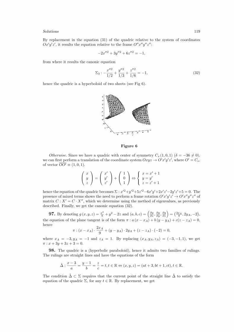
Solutions 119
By replacement in the equation (31) of the quadric relative to the system of coordinatesOx′y′z′, it results the equation relative to the frame O′′x′′y′′z′′:
−2x′′2 + 3y′′2 + 6z′′2 = −1,
from where it results the canonic equation
Σ3 : −x′′2
1/2+y′′2
1/3+z′′2
1/6= −1, (32)
hence the quadric is a hyperboloid of two sheets (see Fig 6).
Figure 6
Otherwise. Since we have a quadric with center of symmetry Cs (1, 0, 1) (δ = −36 = 0),we can first perform a translation of the coordinate system Oxyz → O′x′y′z′, where O′ = Cs,of vector OO′ ≡ (1, 0, 1). x
yz
=
x′
y′
z′
+
101
⇔
x = x′ + 1y = y′
z = z′ + 1
hence the equation of the quadric becomes Σ : x′2+y′2+5z′2−6x′y′+2x′z′−2y′z′+5 = 0. Thepresence of mixed terms shows the need to perform a frame rotation O′x′y′z′ → O′x′′y′′z′′ ofmatrix C : X ′ = C ·X ′′, which we determine using the method of eigenvalues, as previouslydescribed. Finally, we get the canonic equation (32).
97. By denoting g (x, y, z) = x2
9 + y2 − 2z and (a, b, c) =(∂g∂x ,
∂g∂y ,
∂g∂z
)=(2xA
9 , 2yA,−2),
the equation of the plane tangent is of the form π : a (x− xA) + b (y − yA) + c(z − zA) = 0,hence
π : (x− xA) ·2xA9
+ (y − yA) · 2yA + (z − zA) · (−2) = 0,
where xA = −3, yA = −1 and zA = 1. By replacing (xA, yA, zA) = (−3,−1, 1), we getπ : x+ 3y + 3z + 3 = 0.
98. The quadric is a (hyperbolic paraboloid), hence it admits two families of rulings.The rulings are straight lines and have the equations of the form
∆ :x− 3
a=y − 1
b=z
c= t, t ∈ R ⇔ (x, y, z) = (at+ 3, bt+ 1, ct), t ∈ R.
The condition ∆ ⊂ Σ requires that the current point of the straight line ∆ to satisfy theequation of the quadric Σ, for any t ∈ R. By replacement, we get
120 LAAG-DGDE
(at+ 3)2
9− (ct)
2
4= bt+ 1 ⇔
(a2
9− c2
4
)t2 +
(2a
3− b
)t = 0,∀t ∈ R,
hence from the system obtained by canceling the coefficients of the polynomial in t, it resultsb = 2a/3; c = ±2a/3, the solutions v ≡
(a, 2a3 ,±
2a3
)= a
3 (3, 2,±2). According to the twodistinct directions given by the vectors (3, 2,±2), it results that the rulings are given by∆ : x−3
3 = y−12 = z
±2 = t, t ∈ R.The angle θ between the two rulings is the one formed by their director vectors; hence
θ = arccos⟨(3, 2, 2) , (3, 2,−2)⟩
∥(3, 2, 2)∥ · ∥(3, 2,−2)∥= arccos (9/17) .
The plane π which is tangent to the quadric at its pointM(3, 1, 0) can be obtained by halvingthe equation of the quadric with the coordinates the point M . We get
π :x · 39
− z · 04
=1
2(y + 1) ⇔ 2x− 3y − 3 = 0.
The normal straight line ∆′ ∋ M(3, 1, 0) is given by the free vector u ≡ (2,−3, 0) which isnormal to the tangent plane; it results ∆′ : x−3
2 = y−1−3 = z
0 .
III.7. Generated surfaces
99. The cylinder Σ has its ruling lines parallel to the given straight line only if theirequations are of the form
∆′ :x− a
1=y − b
1=z − c
−1⇔{x− y = a− by + z = c− b
⇔{x− y = λy + z = µ,
whereλ = a− b, µ = c− b, λ, µ ∈ R. (33)
We impose ∆′ to lay on the curve
{x = y2
z = 0. This is equivalent to the compatibility of the
system
∆′ ∩Ga :
{x = y2, z = 0x− y = λ, y + z = µ
⇔{x = µ+ λ, z = 0y = µ, x = y2,
hence with the fulfillment of the condition of compatibility λ+µ = µ2. By replacing λ and µgiven by the relations (33) in the obtained condition of compatibility, it results the equationof the claimed cylindric surface
Σ : x− y + y + z = (y + z)2 ⇔ y2 + 2yz + z2 − x− z = 0,
a cylinder parabolic (quadric).
100. The rulings of the conic surface Σ pass all through its vertex V (1, 0, 0), hence theirequations are of the form
∆′ :x− 1
a=y − 0
b=z − 0
c, (a2 + b2 + c2 > 0);
assuming a = 0, by dividing by a and denoting λ = ba , µ = c
a ∈ R, these equations can bewritten as
x− 1
1=y − 0
λ=z − 0
µ⇔{λx− λ = yµx− µ = z,
Solutions 121
whereλ =
y
x− 1, µ =
z
x− 1. (34)
Moreover, the fact that ∆′ lays on the curve Γ :
{x2 + y2 = 1x− z = 0
leads to the compatibility
condition of the system
∆′ ∩ Γ :
{x2 + y2 = 1, x− z = 0
λx− λ = y, µx− µ = z⇔
{x = z = µ
µ−1
y = λµ−1 , x2 + y2 = 1,
namely µ2 + λ2 = (µ− 1)2 ⇔ λ2 + 2µ − 1 = 0. By replacing λ and µ from the relations
(34) in the obtained condition of compatibility, it results the equation of the claimed conicsurface
Σ :
(y2
x− 1
)+ 2
(z
x− 1
)− 1 = 0 ⇔ (x− 1)
2 − 2 (x− 1) z − y2 = 0
hence a cone (a quadric).
101. a) The plane π in which is located the generating circle of the quadric is perpen-dicular on the axis Oy : x0 = y
1 = z0 , hence has the equation of the form πλ : 0 ·x+1 ·y+0 ·z =
λ⇔ y = λ, λ ∈ R. Moreover, the generating circle is included in a sphere Σr with the centeron the axis Oy. Assuming the center of the sphere Σr at C(0, 0, 0) ∈ Oy, then it has theequation Σr : x
2 + y2 + z2 = µ, hence the generator circle has the equations
Γλ,µ :
{y = λx2 + y2 + z2 = µ.
(35)
The fact that this generating circle lays on the director straight line ∆ : x−10 = y+2
2 = z−30
is equivalent with satisfying the compatibility condition of the system{y = λ, x2 + y2 + z2 = µx = 1, z = 3.
(36)
By eliminating x, y, z from the system we get the condition of compatibility
1 + λ2 + 9 = µ⇔ λ2 + 10 = µ.
By replacing λ and µ from the relations (35) in (36) we get the equation of the claimedsurface (a right circular cylinder having as axis of symmetry, the Oy axis): Σ : x2 + z2 = 10.
b) The plane and the sphere which determine the generator circle have the equations y =λ, λ ∈ R, respectively x2 + y2 + z2 = µ, where µ = R2 > 0. We get the condition ofcompatibility of the system {
y = λ, x2 + y2 + z2 = µx = 3y + 6, z = −y − 2,
given by 11λ2 + 40λ+ 40 = µ. By replacing λ and µ from their initial values, it results theequation of the claimed surface, a cone with the symmetry axis-the Oy axis, of equation
Σ : x2 − 10y2 + z2 − 40y + 40 = 0 ⇔ x2 − 10 (y + 2)2+ z2 = 0.
c) In the same manner, we get the compatibility condition 11λ2+34λ+37 = µ, where λ = y,and µ = x2 + y2 + z2, and the obtained surface of revolution is the hyperboloid of one sheet
Σ : x2 − 10y2 + z2 − 34y − 37 = 0 ⇔ x2 − 10
(y +
17
10
)2
+ z2 =81
10.
122 LAAG-DGDE
IV.1. Differentiable mappings
102. a) Let s, t ∈ R. Then
f(s) = f(t) ⇔ (s2, s3) = (t2, t3) ⇔{s2 = t2
s3 = t3⇔ s = t,
and hence f is one-to-one. Let (x, y) ∈ R2 be an arbitrary point from the range of thefunction. Since
f(s) = (x, y) ⇔ (s2, s3) = (x, y) ⇔{s2 = xs3 = y,
and for x < 0 the system has no solutions, it results that the function f is not surjective.Not being surjective, f is not bijective.
b) The Jacobian matrix of the function f = (f1, f2) is
[J(f)] =
( df1ds
df2ds
)=
(2s
3s2
).
Since for s = 0 we have rank [J(f)] = 0 < 1, f is neither an immersion, nor a submersion.Since J(f) is not a quadratic matrix, f cannot be a diffeomorphism.
103. a) The relation f(s) = f(t) can be written 2 cos2 s = 2 cos2 tsin 2s = sin 2t2 sin s = 2 sin t
⇔{
sin s = sin tcos s = ± cos t
and since s, t ∈(0, π2
), it results s = t; hence f is one-to-one. Let (x, y, z) ∈ R3 be an
arbitrary point from the range of the function. Since f(t) = (x, y, z) ⇔
2 cos2 t = xsin 2t = y2 sin t = z
and
since for x ∈ (−∞,−2) ∪ (2,+∞) or y ∈ (−∞,−1) ∪ (1,+∞) or z ∈ (−∞,−2) ∪ (2,+∞),the system has no solutions, it results that the function f is neither surjective and hence norbijective.
b) The Jacobian matrix of the function f is
[J(f)] =
4 cos t · (− sin t)2 cos 2t2 cos t
=
−2 sin 2t2 cos 2t2 cos t
.Since for ∀t ∈ R, we have (−2 sin 2t)2 + (2 cos 2t)2 = 4 = 0, it results rank [J(f)] = 1,hence f is an immersion. Obviously, f is neither a submersion ( rank [J(f)] = 1 = 3), nor adiffeomorphism.
104. a) For (u, v), (s, t) ∈ R2, we have f(u, v) = f(s, t) ⇔{v = s+ t− uu2 − u(s+ t) + st = 0
,
in which the second equation of the system has the solutions (u, v) = (s, t) or (u, v) = (t, s),which show the symmetry of the function f relative to the variables u, v. Since ∀(u, v) ∈ R2,f(u, v) = f(v, u), it results that f is not one-to-one (e.g., f(0, 1) = f(1, 0) = (1, 0)); f is notbijective. On the other hand, we have
f(u, v) = (x, y) ⇔{v = x− uu2 − ux+ y = 0,
Solutions 123
and the second equation admits real solutions only if we have y ≤ x2/4. Hence there existpairs (x, y) ∈ R2 which have no pre-image via f ; hence f is not surjective. For (x, y) = (0, 1)we get
f(u, v) = (0, 1) ⇔{u+ v = 0uv = 1
⇒ u2 = −1,
hence f−1(0, 1) = g� . As well, the condition (x, y) ∈ Im f leads to the equality from above,y ≤ x2/4. Hence, Im f = {(x, y) ∈ R2 | y ≤ x2/4}.
b) The Jacobian matrix of the function f is [J(f)] =
(−1 2v3u2 −1
). We have det[J(f)] =
1 − 6vu2, hence rank [J(f)] = 2 for ∀(u, v) ∈ R2\D, where D = {(u, v)|u2v = 16}, hence
f is both immersion and submersion on R2\D. Using the Theorem of implicit functions,it results that f is a local diffeomorphism, but being bijective, it results that f is a globaldiffeomorphism on R2\D.
105. By denoting f1(ρ, θ) = ρ cos θ and f2(ρ, θ) = ρ sin θ, we get the Jacobian matrix ofthe function f :
J(f) =
∂f1∂ρ
∂f1∂θ
∂f2∂ρ
∂f2∂θ
=
(cos θ −ρ sin θ
sin θ ρ cos θ
).
Since det[J(f)] = ρ cos2 θ+ ρ sin2 θ = ρ > 0, ∀(ρ, θ) ∈ (0,∞)× [0, 2π), using the Theorem ofthe inverse function, it results that f is a diffeomorphism. In order to find the inverse of f ,we solve the following system in the unknowns ρ and θ:{
ρ cos θ = xρ sin θ = y
⇒ ρ2(cos2 θ + sin2 θ) = x2 + y2 ⇒ ρ =√x2 + y2.
We have the following cases:
1o. x = 0, y > 0 ⇒ θ = π/2; 2o. x = 0, y < 0 ⇒ θ = 3π/2; 3o. x > 0, y ≥ 0 ⇒ θ = arctan yx ;
4o. x < 0 ⇒ θ = π + arctan yx ; 5
o. x > 0, y < 0 ⇒ θ = 2π + arctan yx , hence f
−1(x, y) =
(√x2 + y2, θ), where
θ =
kπ + arctan yx , for x = 0,
π/2, for x = 0, y > 03π/2, for x = 0, y < 0,
(37)
where k takes the values 0, 1 and 2 in accordance to the location of the point (x, y) respectivelyin the quadrants I, II or III, or in quadrant IV. We conclude that
f−1(x, y) = (√x2 + y2, θ), f−1 : R2\{(0, 0)} → (0,∞)× [0, 2π),
with the value of the angle θ given by the equality (37).
IV.2. Curves in Rn
106. We find the value of the parameter t0 ∈ R for which α(t0) = (1,−1, 1, 3); from thisequality we get
t40 = 1,−1 = −1, t50 = 1, t60 + 2 = 3,
from where it results t0 = 1. The vector α′(t0) tangent at the point A to the curve hasthe coordinates (4t30, 0, 5t
40, 6t
50) = (4, 0, 5, 6), hence the tangent straight line and the normal
hyperplane at the point A are respectively described by the equations
∆tg,A : x1−14 = x2+1
0 = x3−15 = x4−3
6
Hnor,A : 4(x1 − 1) + 0(x2 + 1) + 5(x3 − 1) + 6(x4 − 3) = 0 ⇔
⇔ 4x1 + 5x3 + 6x4 − 27 = 0.
124 LAAG-DGDE
107. We remark that α(t0) = (0,−1, 0, 2) implies t0 = 0. We haveα′(0) = (4t30, 0, 5t
40, 6t
50) = (0, 0, 0, 0)
α′′(0) = (12t20, 0, 20t30, 30t
40) = (0, 0, 0, 0)
α′′′(0) = (24t0, 0, 60t20, 120t
30) = (0, 0, 0, 0)
α(iv)(0) = (24, 0, 120t0, 360t20) = (24, 0, 0, 0) = (0, 0, 0, 0),
hence it results that B is a singular point of order 4. We conclude that the tangent straightline and the normal hyperplane to the curve α at the point B are respectively described bythe equations
∆tg,B : x1−024 = x2+1
0 = x3−00 = x4−2
0 ⇔
x2 = −1x3 = 0x4 = 2
Hnor,B : 24 · (x1 − 0) + 0 · (x2 + 1) + 0 · (x3 − 0) + 0 · (x4 − 2) = 0 ⇔ x1 = 0.
From the relation α′(t) = 0 it results the unique solution t = 0, hence B is the uniquesingular point of the curve.
108. We find the common points of the curves by solving the system α(t) = β(s), whichcan be written {
t2 + 1 = 2 + sln t = s, t = s+ 1
⇔{s2 + s = 0ln t = s, t = s+ 1
⇔{s = 0t = 1,
hence the common point of the curves is α(1) = β(0) = (2, 0, 1). The tangent vectors at thecommon point to the pair of curves, are α′(1) = (2, 1, 1), respectively β′(0) = (1, 1, 1), hencewe have
(α′(1), β′(0)) = arccos⟨α′(1), β′(0)⟩
∥α′(1)∥ · ∥β′(0)∥= arccos
4
3√2.
109. By denoting x(t) = t− 1, y(t) = t2
t−1 , we get
limt→−∞
x(t) = −∞, limt→−∞
y(t) = −∞,
limt→+∞
x(t) = ∞, limt→+∞
y(t) = ∞,
and since limt→±∞
y(t)
x(t)= lim
t→±∞
t2
(t− 1)2= 1 = m, it results that v ≡ (1, 1) is an asymptotic
direction of the curve for t → ±∞. Since n = limt→±∞
(y(t)−m · x(t)) = limt→±∞
2t− 1
t− 1= 2 it
results that y = x+ 2 an asymptotic line a of the curve for t→ ±∞.At the accumulation point t = 1, we have
limt→1
x(t) = 0, limt↗1
y(t) = −∞, limt↘1
y(t) = +∞,
hence the curve admits for t→ 1 the bi-lateral asymptotic line x = 0 (the Oy axis).
110. a) According to the definition, the length of the curve segment is
l = α([0, 2π]) =
∫ 2π
0
∥α′(t)∥dt.
Solutions 125
We have α′(t) = (a(1− cos t), a · sin t), hence
∥α′(t)∥ =
√a2(1− cos t)2 + a2 · sin2 t = a
√2− 2 cos t.
Using the relation cos t = 1− 2 sin2 t2 , it results
l = a
∫ 2π
0
√2− 2 cos tdt = a
∫ 2π
0
√2− 2
(1− 2 sin2
t
2
)dt.
But t ∈ [0, 2π] ⇔ t2 ∈ [0, π] ⇒ sin t ≥ 0, hence
l = 2a
∫ 2π
0
sint
2dt = −4a cos · t
2
∣∣∣∣2π0
= −4a(−1− 1) = 8a.
b) Since the origin α(0) = (0, 0) is not a regular point of the curve α (since α′(0) = 0), weshall compute the normal parameter which corresponds to t = π. We have
s(t) =
∫ t
π
∥α′(u)∥du = a
∫ t
π
√2− 2 cosu du = 2a
∫ t
π
sinu
2du =
= −4a · cos .u2
∣∣∣∣tπ
= −4a cos t2 , s : [0, 2π] → [−4a, 4a].
We remark that the inverse of the function, t : [−4a, 4a] → [a, 2π] is given by t(s) =2 arccos(− s
4a ). We conclude that the normal parameterization of the curve α is β : [−4a, 4a] →R2,
β(s) = (α ◦ s−1)(s) = α(s−1(s)) = α(2 arccos(− s4a )) =
= (a(2 arccos(− s4a )− sin(2 arccos(− s
4a ))), a(1− cos(2 arccos(− s4a )))).
IV.3. Planar curves
111. From the relation α(t) = A it results t = −1. But α′(−1) ≡ (−2, 3) = 0, and theequations of the tangent and normal straight lines at A respectively are
∆tg :x−1−2 = y+3
3 ⇔ 3x+ 2y + 3 = 0
∆nor : −2(x− 1) + 3(y + 3) = 0 ⇔ −2x+ 3y + 11 = 0.
The intersection point T of the tangent straight line with the Ox axis is the solution of thesystem
∆tg ∩Ox :
{3x+ 2y + 3 = 0y = 0
⇔{x = −1y = 0
⇒ T (−1, 0).
By denoting with C the projection of the point A(1,−3) on the Ox axis, the sub-tangent is
St =√AT 2 −AC2 =
√13− 9 = 2. We find the intersection point N of the normal with the
Ox axis, given by
∆nor ∩Ox :
{−2x+ 3y + 11 = 0y = 0
⇔{x = 11/2y = 0
⇒ N(11/2, 0).
We conclude that the sub-normal is
Sn =√AN2 −AC2 =
√117
4− 9 =
9
2.
126 LAAG-DGDE
112. a) We denote F (x, y) = x2− y3−3 and (xA, yA) = (−2, 1). Using the formulas forthe tangent and normal straight line to a plane curve given by implicit Cartesian equation,
∆tg : (x− xA) ·(∂F∂x
)(xA,yA)
+ (y − yA) ·(∂F∂y
)(xA,yA)
= 0,
∆nor :x− xA
(∂F∂x )(xA,yA)
=y − yA
(∂F∂y )(xA,yA)
.
We get ∆tg : 4x+ 3y + 5 = 0, respectively ∆nor :x+2−4 = y−1
−3 .
b) We have x2 − y3 − 3 = 0 ⇒ y = 3√x2 − 3, hence a parameterization a of the curve α is{x = t
y = 3√t2 − 3
, t ∈ R.
113. a) The basis of the Frenet frame RF = {α(t); {T (t), N(t)}} of the curve α is given
by the pair of vector fields {T , N}, where:T (t) ≡ α′(t)
∥α′(t)∥ =
(x′(t)√
x′2(t)+y′2(t), y′(t)√
x′2(t)+y′2(t)
)N(t) = Rπ/2(T (t)) ≡
(−y′(t)√
x′2(t)+y′2(t), x′(t)√
x′2(t)+y′2(t)
).
In our case x(t) = t, y(t) = t2, hence x′(t) = 1, y′(t) = 2t. It follows that
T (t) =
(1√
1 + 4t2,
2t√1 + 4t2
), N(t) =
(− 2t√
1 + 4t2,
1√1 + 4t2
).
Since α′(t) = (1, 2t) = OR2 , it results that α is a regular curve and hence the value of thecurvature of the curve is given by the equality
k(t) =x′(t)y′′(t)− x′′(t)y′(t)
(x′2(t) + y′2(t))3/2=
1 · 2− 0 · 2t(1 + 4t2)3/2
=2
(1 + 4t2)3/2. (38)
b) The Frenet frame of the curve α at the current point α(t) is RF = {α(t); {T (t), N(t)}},where T (t) = α′(t)
∥α′(t)∥ and N(t) = Rπ2T (t) are the unit vector tangent and respectively normal
to the curve α at the point α(t). These unit vectors, considered at the point A ∈ Imα willbe denoted by TA, NA. As α(t) = (t, t2) it results α′(t) = (1, 2t). We have A ∈ Imα, sinceA(−2, 4) = α(−2). Since α′(−2) = (1,−4) has its norm ∥α′(−2)∥ =
√17 = 0, the point A is
a regular point of the curve α. The claimed unit vectors are:TA = α′(−2)
∥α′(−2)∥ = ( 1√17,− 4√
17)
NA = Rπ2TA ≡
(cos π
2− sin π
2
sin π2
cos π2
)( 1√17
− 4√17
)=
(4√171√17
),
hence the associated Frenet frame of the curve α at the point A(−2, 4) is
RF,A =
{A(−2, 4);
{TA =
(1√17,− 4√
17
), NA =
(4√17,
1√17
)}}.
Using the relation (38), for t = tA = −2, we get the value of the curvature at the pointA(−2, 4) = α(−2), k(−2) = 2
17√17.
Solutions 127
c) We find the equation of the osculating circle at the point A = α(−2) using the formula(x− x0)
2 + (y − y0)2 = R2
0, where
x0 = xC(−2), y0 = yC(−2), R0 = R(−2) =1
|k(−2)|,
and the coordinates of the center of the osculating circle to the curve at the current pointα(t) = (x(t), y(t)) are given by xC(t) = x(t)− y′(t) · x′2(t)+y′2(t)
x′(t)y′′(t)−x′′(t)y′(t) = −4t3
yC(t) = y(t) + x′(t) · x′2(t)+y′2(t)x′(t)y′′(t)−x′′(t)y′(t) =
1+6t2
2 .(39)
The curvature function k(t) at α(t) is given by the relation (38), hence the radius of theosculating circle is
R(t) =1
|k(t)|=
(1 + 4t2)3/2
2.
In item α(−2), we get, by replacing t = −2:
x0 = −4 · (−2)3 = 32, y0 =1 + 6 · (−2)2
2=
25
2, R0 =
17√17
2.
We conclude that the equation of the osculating circle to the curve α at the point A = α(−2)is (x− 32)2 + (y − 25
2 )2 = 49134 .
d) Using the formulas (39) we get the parameterization of the evolute:
αev(t) =
(−4t3,
6t2 + 1
2
), t ∈ R.
e) We get the Cartesian equation a of the curve α by eliminating the parameter t from the
system
{x = ty = t2
. By replacing the obtained value of t from the first relation in the second,
we get Γ = Imα : x2 − y = 0 ⇒ y = x2, i.e., a parabola.
114. a) Denoting x = t, we get for Γ the parameterization α : R → R2, α(t) = (t, t2), t ∈R. Then
k(t) =
∣∣∣∣ x′ y′
x′′ y′′
∣∣∣∣(√x′2 + y′2
)3 =
∣∣∣∣ 1 2t0 2
∣∣∣∣(√1 + (2t)
2
)3 =2
(1 + 4t2)3/2.
But α(t) = A⇔ (t, t2) = (2, 4) ⇔ t = 2, hence the claimed curvature is k(2) = 217
√17.
b) The explicit Cartesian equation of the curve α is y = f(x), where f(x) = x2. Then
k(x) =f ′′(x)(√
1 + (f ′(x))2)3 =
2
(√1 + (2x)2)3
,
and for x = 2 we get k(2) = 217
√17.
c) Because y = x2 ⇔ x2 − y = 0, the implicit Cartesian equation of the curve Γ isF (x, y) = 0, where F (x, y) = x2 − y. Then
k(x, y) = −sign(Fy) ·FxxF
2y + FyyF
2x − 2FxxFxFy(
F 2x + F 2
y
)3/2 ,
128 LAAG-DGDE
where Fx = ∂F/∂x, Fy = ∂F/∂y etc, and hence
k(x, y) = −sign(−1) · 2 · (−1)2 + 0 · (2x)2 − 2 · 0 · 2x · (−1)
[(2x)2 + (−1)2]3/2=
2
(1 + 4x2)3/2
,
which leads to k(2, 4) = 217
√17.
115. a) By denoting F (x, y, a) = (x− a)2 + y2 − a2
2 , the envelope of the family of planecurves Γa : F (x, y, a) = 0 (if this exists) is contained in the curve Γ∗ defined by the system{
F (x, y, a) = 0
∂F∂a (x, y, a) = 0, a ∈ R,
which in our case becomes{(x− a)2 + y2 − a2
2 = 0−2(x− a)− a = 0
⇔{a = 2x
(x− a)2 + y2 − a2
2 = 0
from which, by eliminating on a, we get Γ∗ : x2 − y2 = 0 or x = ±y, hence the curve Γ∗ isthe union of the two bisectors y = x and y = −x.b) We proceed as in item a); the envelope of the family of curves Γα : x · cosα+ y · sinα = 2is contained in the curve Γ∗ defined by the system{
x · cosα+ y · sinα = 2−x · sinα+ y · cosα = 2, α ∈ R.
Multiplying with cosα the first relation and with − sinα the second relation, and then, withsinα the first relation and with cosα the second one and summing them up, we get{
x = 2(cosα− sinα)y = 2(cosα+ sinα)
from which, by eliminating the variable α via summing the squares, we get Γ∗ : x2 + y2 = 4,hence the curve Γ∗ is the circle with the center at the origin having the radius 2.
c) The envelope of the family of curves Γλ : x2 + y2 − 2λx+ λ2 − 4λ = 0 is contained in thecurve Γ∗ defined by the system:{
x2 + y2 − 2λx+ λ2 − 4λ = 0−2x+ 2λ− 4 = 0
⇔{λ = x+ 2x2 + y2− 2λx+ λ2 − 4λ = 0,
from which, by eliminating the variable λ, we get Γ∗ : y2 − 4x = 4 ⇔ y2 = 4(x+ 1), hence aparabola with the vertex on the Ox axis, which admits Ox as axis of symmetry.
116. a) We use the formulas of tangent, respectively normal to the curve Γ : F (x, y) = 0at the point (x0, y0) ∈ Γ,
∆tg : (x− x0) ·∂f
∂x(x0, y0) + (y − y0) ·
∂f
∂y(x0, y0) = 0
∆nor :x− x0
∂f∂x (x0, y0)
=y − y0
∂f∂y (x0, y0)
.
For (x0, y0) = (2,−1) and f(x, y) = x3−2y2 we get the equations of the tangent, respectivelyof the normal straight lines
∆tg : 3x+ y − 5 = 0, ∆nor :x− 2
3=y + 1
1⇔ x− 3y − 5 = 0.
Solutions 129
b) The singular points of the curve Γ are the solutions of the systemf(x, y) = 0
∂f∂x (x, y) = 0
∂f∂y (x, y) = 0
⇔
x3 − 2y2 = 03x2 = 0−4y = 0
⇒{x = 0y = 0,
hence O(0, 0) is the unique singular point of the curve. Since
det[Hess(f)]O =
∣∣∣∣∣∣∂2f∂x2 (0, 0)
∂2f∂x∂y
(0, 0)
∂2f∂x∂y
(0, 0) ∂2f∂y2 (0, 0)
∣∣∣∣∣∣ =∣∣∣∣ 0 00 −4
∣∣∣∣ = 0,
where f(x, y) = x3 − 2y2, it results that O(0, 0) is a cusp singular point of the curve Γ. Thedirection v = (l,m) tangent at O(0, 0) to the curve is given by the relation
l2 · ∂2f
∂x2(0, 0) + 2l ·m · ∂2f
∂x∂y(0, 0) +m2 · ∂
2f
∂y2(0, 0) = 0 ⇔ m2 · (−4) = 0 ⇔ m = 0,
and hence v = l(1, 0). We conclude that the equations of the tangent, respectively of thenormal to the curve Γ at its point O(0, 0) ∈ Γ, are
∆tg :x−01 = y−0
0 ⇔ y = 0, (the Ox axis)
∆nor : 1 · x− 0 + 0 · (y − 0) = 0 ⇔ x = 0, (the Oy axis).
Γ is not a regular curve, since it contains singular points.
117. We follow several preliminary steps.
i) The definition domain is Dα = (−∞, 0) ∪ (0,∞). We remark that 0 /∈ Dα, and
Γ ∩Ox : 2 + t+1
t= 0 ⇔ t2 + 2t+ 1 = 0 ⇔ t = −1,
and then Γ ∩Ox = {α(−1)} = {(2, 0)}. As well,
Γ ∩Oy : 2− t+1
t= 0 ⇔ t2 − 2t− 1 = 0 ⇔ t = 1±
√2,
hence Γ ∩Oy = {α(1±√2)} = {(0, 2± 2
√2)}.
ii) We study if α is o periodic curve, hence if ∃T > 0, α(t) = α(t+ T ), ∀t ∈ Dα s.t.t+ T ∈ Dα. We have { 1
t = −T + 1t+T
1t = T + 1
t+T , ∀t ∈ R∗⇔ T = 0.
It follows that α is not a periodic curve.iii) We find the asymptotic behavior of the curve Γ = Imα (asymptotic points; horizontal,slant or vertical asymptotic lines). Since Dα = (−∞, 0) ∪ (0,+∞), we perform this studyonly for t0 = {±∞, 0} (hence at the accumulation points which do not belong to the definitiondomain of the curve).
We compute the limits at the accumulation points from R which do not belong to thedomain of the curve, t0 ∈ Dα = {±∞, 0−, 0+}. We have
limt→−∞
α(t) = (+∞,−∞), limt→+∞
α(t) = (−∞,+∞),
limt↗0
α(t) = (−∞,−∞), limt↘0
α(t) = (+∞,+∞),
130 LAAG-DGDE
hence α does not admit horizontal or vertical asymptotic lines. For t → ±∞, t ↗ 0 andt ↘ 0 there exist infinite branches. We study the existence of slant asymptotic lines. Wehave:
m = limt→±∞
y(t)
x(t)= limt→±∞
t(1 + 2t +
1t2 )
t(−1 + 2t +
1t2 )
= −1
n = limt→±∞
(y(t) + x(t)) = limt→±∞
(4 +2
t) = 4.
It follows that the straight line ∆as,±∞ : y = −x+ 4 is a slant asymptotic line of the curvefor t→ ±∞. As well,
m = limt→0
y(t)
x(t)= limt→0
t2 + 2t+ 1
t2 − 2t+ 1= 1
n = limt→0
(y(t)− x(t)) = limt→0
2t = 0,
hence the straight line ∆as,0 : y = x is a slant asymptotic line of the curve for t → 0− andfor t→ 0+.iv) We study the existence of the singular points and the extremal points for the coordinate
functions of the curve. We have x′(t) = − t2+1t2 , y′(t) = − t2−1
t2 . We remark that sincex′(t) < 0, ∀x = 0, we have α′(t) = (0, 0), ∀t = 0, hence the curve α is a regular curve.The equation x′(t) = 0 has no solutions, and the equation y′(t) = 0, which implies t2 − 1 =0 ⇔ t = ±1, hence α(−1) = (2, 0) and α(1) = (2, 4) are local extremum points for y(t).v) We study the existence of multiple points α(t1) = α(t2), t1 = t2; t1, t2 ∈ Dα = R∗. Thisrelation leads to the system{
x(t1) = x(t2)
y(t1) = y(t2)⇒
{−t1 + 1
t1+ t2 − 1
t2= 0
t1 +1t1
− t2 − 1t2
= 0
in the unknown t2, with t1 regarded as a parameter. Subtracting the two relations, we gett2 = t1, hence the curve α has no multiple points.vi) We study the existence of inflexion points. By direct calculation, it results that the
equation α′(t) = λ · α′′(t) is equivalent to the system
{− t2−1
t2 = λ · 2t3
t2−1t2 = λ · 2
t3
, which are the
unknowns t ∈ Dα, λ ∈ R. This has no solutions (t, λ) ∈ Dα × R (e.g., subtracting theequations we get −2 = 0), hence the curve has no inflexion points.vii) The variation table of the curve α is (see Fig 7):
t −∞ −1 1 −√
2 0 1 1 +√
2 +∞x(t) +∞ ↘ 2 ↘ 0 ↘ −∞|∞ ↘ 2 ↘ 0 ↘ −∞y(t) −∞ ↗ 0 ↘ 2 − 2
√2 ↘ −∞|∞ ↘ 4 ↗ 2 + 2
√2 ↗ +∞
x′(t) − − −1 − − − −|− − −1 − − − −y′(t) + + 0 − − − −|− − 0 + + + +
Obs. y = −x + 4 My A y = x|y = −x my B y = −x + 4
118. a) For the curve Γ1 : y2(a− x) − x3 = 0, the equation of the curve is equivalentwith Γ1 : y2a− x(x2 + y2) = 0. We denote y = t · x and by replacing in the equation of thecurve, we get
at2x2 − t2x3 − x3 = 0 ⇔ x2(x+ xt2 − at2) = 0.
We have the following cases:
i) for x = 0 we have y = 0, hence we get item A(0, 0) ∈ Γ;
ii) for x = 0 we have x+ xt2 − at2 = 0, hence x = at2
1+t2 and y = at3
1+t2 . It follows that for thecurve Γ1 we have the parameterization (see Fig 8):
α1 : R → R2, α1(t) = (x(t), y(t)) =
(at2
1 + t2,at3
1 + t2
), t ∈ R.
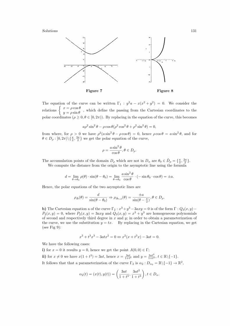
Solutions 131
Figure 7 Figure 8
The equation of the curve can be written Γ1 : y2a − x(x2 + y2) = 0. We consider the
relations
{x = ρ cos θy = ρ sin θ
, which define the passing from the Cartesian coordinates to the
polar coordinates (ρ ≥ 0, θ ∈ [0, 2π)). By replacing in the equation of the curve, this becomes
aρ2 sin2 θ − ρ cos θ(ρ2 cos2 θ + ρ2 sin2 θ) = 0,
from where, for ρ > 0 we have ρ2(a sin2 θ − ρ cos θ) = 0, hence ρ cos θ = a sin2 θ, and forθ ∈ Dρ : [0, 2π)\{π2 ,
3π2 } we get the polar equation of the curve,
ρ =a sin2 θ
cos θ, θ ∈ Dρ.
The accumulation points of the domain Dρ which are not in Dα are θ0 ∈ Dρ = {π2 ,3π2 }.
We compute the distance from the origin to the asymptotic line using the formula
d = limθ→θ0
ρ(θ) · sin(θ − θ0) = limθ→θ0
a sin2 θ
cos θ· (− sin θ0 · cos θ) = ±a.
Hence, the polar equations of the two asymptotic lines are
ρ∆(θ) =d
sin(θ − θ0)⇒ ρ∆1,2(θ) =
±asin(θ − π
2 ), θ ∈ Dρ.
b) The Cartesian equation a of the curve Γ2 : x3+y3−3axy = 0 is of the form Γ : Q3(x, y)−P2(x, y) = 0, where P2(x, y) = 3axy and Q3(x, y) = x3 + y3 are homogeneous polynomialsof second and respectively third degree in x and y; in order to obtain a parameterization ofthe curve, we use the substitution y = tx. By replacing in the Cartesian equation, we get(see Fig 9):
x3 + t3x3 − 3atx2 = 0 ⇔ x2(x+ t3x)− 3at = 0.
We have the following cases:
i) for x = 0 it results y = 0, hence we get the point A(0, 0) ∈ Γ;
ii) for x = 0 we have x(1 + t3) = 3at, hence x = 3at1+t3 and y = 3at2
1+t3 , t ∈ R\{−1}.It follows that that a parameterization of the curve Γ2 is α2 : Dα2 = R\{−1} → R2,
α2(t) = (x(t), y(t)) =
(3at
1 + t3,3at2
1 + t3
), t ∈ Dα.
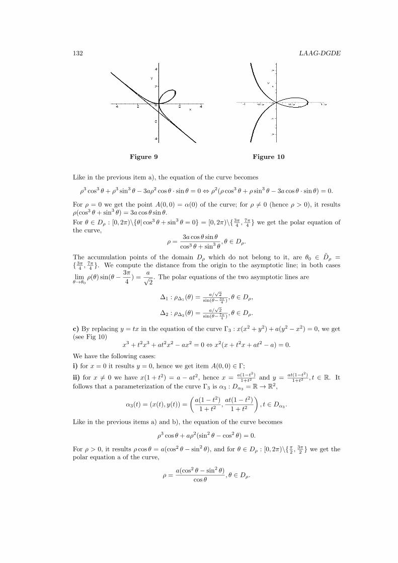
132 LAAG-DGDE
Figure 9 Figure 10
Like in the previous item a), the equation of the curve becomes
ρ3 cos3 θ + ρ3 sin3 θ − 3aρ2 cos θ · sin θ = 0 ⇔ ρ2(ρ cos3 θ + ρ sin3 θ − 3a cos θ · sin θ) = 0.
For ρ = 0 we get the point A(0, 0) = α(0) of the curve; for ρ = 0 (hence ρ > 0), it resultsρ(cos3 θ + sin3 θ) = 3a cos θ sin θ.
For θ ∈ Dρ : [0, 2π)\{θ| cos3 θ + sin3 θ = 0} = [0, 2π)\{ 3π4 ,
7π4 } we get the polar equation of
the curve,
ρ =3a cos θ sin θ
cos3 θ + sin3 θ, θ ∈ Dρ.
The accumulation points of the domain Dρ which do not belong to it, are θ0 ∈ Dρ ={ 3π
4 ,7π4 }. We compute the distance from the origin to the asymptotic line; in both cases
limθ→θ0
ρ(θ) sin(θ − 3π
4) =
a√2. The polar equations of the two asymptotic lines are
∆1 : ρ∆1(θ) =a/
√2
sin(θ− 3π4 ), θ ∈ Dρ,
∆2 : ρ∆2(θ) =a/
√2
sin(θ− 7π4 ), θ ∈ Dρ.
c) By replacing y = tx in the equation of the curve Γ3 : x(x2 + y2) + a(y2 − x2) = 0, we get(see Fig 10)
x3 + t2x3 + at2x2 − ax2 = 0 ⇔ x2(x+ t2x+ at2 − a) = 0.
We have the following cases:
i) for x = 0 it results y = 0, hence we get item A(0, 0) ∈ Γ;
ii) for x = 0 we have x(1 + t2) = a − at2, hence x = a(1−t2)1+t2 and y = at(1−t2)
1+t2 , t ∈ R. It
follows that a parameterization of the curve Γ3 is α3 : Dα3 = R → R2,
α3(t) = (x(t), y(t)) =
(a(1− t2)
1 + t2,at(1− t2)
1 + t2
), t ∈ Dα3
.
Like in the previous items a) and b), the equation of the curve becomes
ρ3 cos θ + aρ2(sin2 θ − cos2 θ) = 0.
For ρ > 0, it results ρ cos θ = a(cos2 θ − sin2 θ), and for θ ∈ Dρ : [0, 2π)\{π2 ,3π2 } we get the
polar equation a of the curve,
ρ =a(cos2 θ − sin2 θ)
cos θ, θ ∈ Dρ.
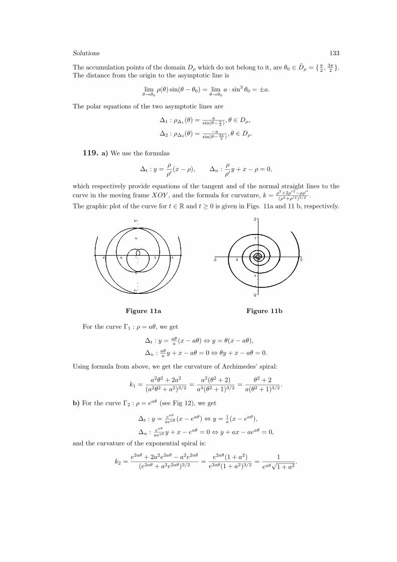
Solutions 133
The accumulation points of the domain Dρ which do not belong to it, are θ0 ∈ Dρ = {π2 ,3π2 }.
The distance from the origin to the asymptotic line is
limθ→θ0
ρ(θ) sin(θ − θ0) = limθ→θ0
a · sin3 θ0 = ±a.
The polar equations of the two asymptotic lines are
∆1 : ρ∆1(θ) =a
sin(θ−π2 ) , θ ∈ Dρ,
∆2 : ρ∆2(θ) =−a
sin(θ− 3π2 ), θ ∈ Dρ.
119. a) We use the formulas
∆t : y =ρ
ρ′(x− ρ), ∆n :
ρ
ρ′y + x− ρ = 0,
which respectively provide equations of the tangent and of the normal straight lines to the
curve in the moving frame XOY , and the formula for curvature, k = ρ2+2ρ′2−ρρ′′(ρ2+ρ′2)3/2
.
The graphic plot of the curve for t ∈ R and t ≥ 0 is given in Figs. 11a and 11 b, respectively.
Figure 11a Figure 11b
For the curve Γ1 : ρ = aθ, we get
∆t : y = aθa (x− aθ) ⇔ y = θ(x− aθ),
∆n : aθa y + x− aθ = 0 ⇔ θy + x− aθ = 0.
Using formula from above, we get the curvature of Archimedes’ spiral:
k1 =a2θ2 + 2a2
(a2θ2 + a2)3/2=
a2(θ2 + 2)
a3(θ2 + 1)3/2=
θ2 + 2
a(θ2 + 1)3/2.
b) For the curve Γ2 : ρ = eaθ (see Fig 12), we get
∆t : y = eaθ
aeaθ (x− eaθ) ⇔ y = 1a (x− eaθ),
∆n : eaθ
aeaθ y + x− eaθ = 0 ⇔ y + ax− aeaθ = 0,
and the curvature of the exponential spiral is:
k2 =e2aθ + 2a2e2aθ − a2e2aθ
(e2aθ + a2e2aθ)3/2=
e2aθ(1 + a2)
e3aθ(1 + a2)3/2=
1
eaθ√1 + a2
.
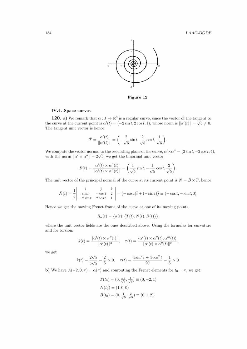
134 LAAG-DGDE
Figure 12
IV.4. Space curves
120. a) We remark that α : I → R3 is a regular curve, since the vector of the tangent tothe curve at the current point is α′(t) = (−2 sin t, 2 cos t, 1), whose norm is ∥α′(t)∥ =
√5 = 0.
The tangent unit vector is hence
T =α′(t)
∥α′(t)∥=
(− 2√
5sin t,
2√5cos t,
1√5
).
We compute the vector normal to the osculating plane of the curve, α′×α′′ = (2 sin t,−2 cos t, 4),with the norm ∥α′ × α′′∥ = 2
√5; we get the binormal unit vector
B(t) =α′(t)× α′′(t)
∥α′(t)× α′′(t)∥=
(1√5sin t,− 1√
5cos t,
2√5
).
The unit vector of the principal normal of the curve at its current point is N = B× T , hence
N(t) =1
5
∣∣∣∣∣∣i j k
sin t − cos t 2−2 sin t 2 cos t 1
∣∣∣∣∣∣ = (− cos t)i+ (− sin t)j ≡ (− cos t,− sin t, 0).
Hence we get the moving Frenet frame of the curve at one of its moving points,
Rα(t) = {α(t); {T (t), N(t), B(t)}},
where the unit vector fields are the ones described above. Using the formulas for curvatureand for torsion:
k(t) =∥α′(t)× α′′(t)∥
∥α′(t)∥3, τ(t) =
⟨α′(t)× α′′(t), α′′′(t)⟩∥α′(t)× α′′(t)∥2
,
we get
k(t) =2√5
5√5=
2
5> 0, τ(t) =
4 sin2 t+ 4 cos2 t
20=
1
5> 0.
b) We have A(−2, 0, π) = α(π) and computing the Frenet elements for t0 = π, we get:
T (t0) = (0, −2√5, 1√
5) ≡ (0,−2, 1)
N(t0) = (1, 0, 0)
B(t0) = (0, 1√5, 2√
5) ≡ (0, 1, 2).
Solutions 135
c) The curve α is a helix if the ratio between the curvature and the torsion is constant; in
our case, we have k(t)/τ(t) = 2/51/5 = 2 = const.. We conclude that the curve α is a helix.
d) We obtain the Cartesian equations of the curve α by eliminating the parameter t from
the system
x = 2 cos ty = 2 sin tz = t
. By adding the squares of the two relations, we get x2 + y2 = 4
and by replacing t from the last equations into the first one, it results x = 2 cos z, and hence
T = Imα :
{x = 2 cos zx2 + y2 = 4.
e) The edges of the Frenet frame at a current point of the curve, are straight lines: tangent,of the principal normal and binormal. These respectively have the director unit vectorsT (t), N(t), B(t). Their Cartesian equations are
∆tg :x− 2 cos t
− 2√5sin t
=y − 2 sin t
2√5cos t
=z − t
1√5
∆nor.pr. :x− 2 cos t
− cos t=y − 2 sin t
− sin t=z − t
0
∆bin :x− 2 cos t
1√5sin t
=y − 2 sin t
− 1√5cos t
=z − t
2√5
.
121. a) The equation of the osculating plane (determined by the current point α(t) andby the vectors α′(t) and α′′(t), is
πosc,α(t) :
∣∣∣∣∣∣x− x(t) y − y(t) z − z(t)x′(t) y′(t) z′(t)x′′(t) y′′(t) z′′(t)
∣∣∣∣∣∣ = 0 ⇔
∣∣∣∣∣∣x− (t2 + t) y − (t2 − t) z − (t2 − t)
2t+ 1 2t− 1 2t− 12 2 2
∣∣∣∣∣∣ = 0 ⇔
⇔ −4(y − (t2 − t)) + 4(z − (t2 − t)) = 0 ⇔ y − z = 0.
Hence the equation of the osculating plane does not depend on the parameter t and henceα is a plane curve. We find the plane π ⊃ Imα.
Let π : ax+ by+ cz+d = 0, a2+ b2+ c2 = 0; we assume that α is included in the plane π.Since α(t) = (t2 + t, t2 − t, t2 − t), t ∈ R, by replacing in the equation of the plane we have
a(t2 + t) + b(t2 − t) + c(t2 − t) + d = 0, ∀t ∈ R ⇔
⇔ t2(a+ b+ c) + t(a− b− c) + d = 0, ∀t ∈ R ⇔
⇔
a+ b+ c = 0a− b− c = 0d = 0
⇔
{a = 0, b = λ,
c = −λ, d = 0λ ∈ R.
The solutions of the system are hence (a, b, c, d) = λ(0, 1,−1, 0), λ ∈ R. By choosing λ = 1,we get the equation of the claimed plane in which is contained the curve, π : y − z = 0. Wenotice that the obtained plane is exactly the osculating plane, hence
Γ = Imα ⊂ π = πosc,α(t).
b) We have
α′(t) = (2t+ 1, 2t− 1, 2t− 1)α′′(t) = (2, 2, 2)α′′′(t) = (0, 0, 0)
, hence ⟨α′, α′′ × α′′′⟩ = 0 and the torsion of
the curve α at the current point becomes:
τ =⟨α′, α′′ × α′′′⟩∥α′ × α′′∥2
= 0, ∀t ∈ R.
136 LAAG-DGDE
c) We have
α′(t)× α′′(t) =
∣∣∣∣∣∣i j k
2t+ 1 2t− 1 2t− 12 2 2
∣∣∣∣∣∣ = 0 · i− 4 · j + 4 · k ≡ (0,−4, 4),
hence the field of the unit vectors of the binormal is
B(t) =α′(t)× α′′(t)
∥α′(t)× α′′(t)∥=
1
4√2(0,−4, 4) =
(0,−
√2
2,
√2
2
).
which obviously does not depend on t.
122. a) For a space curve which is given by its implicit Cartesian equations, Γ :{F (x, y, z) = 0G(x, y, z) = 0
, the equations of the tangent straight lines and the equation of the normal
plane are respectively
∆tg,A :x− x0a
=y − y0b
=z − z0c
πnor,A : a(x− x0) + b(y − y0) + c(z − z0) = 0.
where n = ai + bj + ck = (degF × degG)|A. In our case, F (x, y, z) = x2 + y2 + z2 −2, G(x, y, z) = z − 1 and
n = (degF × degG)|A =
∣∣∣∣∣∣i j k2x 2y 2z0 0 1
∣∣∣∣∣∣∣∣∣∣A(−1,0,1)
=
=
∣∣∣∣∣∣i j k−2 0 20 0 1
∣∣∣∣∣∣ ≡ (0, 2, 0) = (a, b, c).
Hence
∆tg,A : x+10 = y−0
2 = z−10 ⇔
{x = −1z = 1
πnor,A : (x+ 1) · 0 + (y − 0) · 2 + (z + 1) · 0 = 0 ⇔ y = 0 (the plane xOz).
b) In the system Γ :
{x2 + y2 + z2 = 2z = 1
by replacing z from the second the equation in
the first, we get x2 + y2 = 1, hence a parameterization of the curve is
Γ :
x = cos ty = sin tz = 1
, t ∈ [0, 2π).
IV.5. Surfaces
123. a) The partial velocities are the partial derivatives of the function r,{ru = ∂r
∂u = (cos v, sin v, 2u)
rv =∂r∂v = (−u sin v, u cos v, 0).
Solutions 137
The mapping r is a parameterization if it is immersion one-to-one. We check its injectivity.For (u1, v1), (u2, v2) ∈ D, using the fact that u > 0, we get
r(u1, v1) = r(u2, v2) ⇔
u1 cos v1 = u2 cos v2u1 sin v1 = u2 sin v2u21 = u22
⇔{u1 = u2v1 = v2
⇔ (u1, v1) = (u2, v2),
(40)hence r is one-to-one. We check that r is an immersion. We have
dr = ru · du+ rv · dv = [ru, rv]r(u,v) ·(dudv
).
We build the Jacobian matrix [J(r)] = [ru, rv]r(u,v) of the mapping r and check if rank [J(r)] =2. We get
[J(r)] =
cos v −u sin vsin v u cos v2u 0
,
and then ∣∣∣∣ cos v −u sin vsin v u cos v
∣∣∣∣ = u > 0 ⇒ rank [J(r)] = 2,
hence r is immersion; being one-to-one too, it results that r is a parameterization. It resultsthat Σ = r(D) is a simple surface (see Fig 10).
b) We find the parameters u and v associated to the point A ∈ Σ. We solve the system
r(u, v) = A⇔ (u cos v, u sin v, u2) = (−2, 0, 4) ⇔
u cos v = −2u sin v = 0u2 = 4
⇒{u = 2v = π
⇒ A = r(2, π).
We compute the partial velocities in item A.{ru|A = (cosπ, sinπ, 22) = (−1, 0, 4)rv|A = (−2 sinπ, 2 cosπ, 0) = (0,−2, 0).
Then we have
πtg,A :
∣∣∣∣∣∣x+ 2 y z − 4−1 0 40 −2 0
∣∣∣∣∣∣⇔ 4x+ z + 4 = 0.
Hence, a vector which is normal to the plane is n = vnor ≡ (4, 0, 1), and ∆nor,A : x+24 =
y0 = z−4
1 . Otherwise. We find the director vector n of the straight line ∆nor,A.
n = ru×rv =
∣∣∣∣∣∣i j k
cos v sin v 2u−u sin v u cos v 0
∣∣∣∣∣∣∣∣∣∣A=r(2,π)
= (−2u2 cos v,−2u2 sin v, u)u=2,v=π = (8, 0, 2),
from where it results
∆nor,A : x+28 = y
0 = z−42
πtg,A : 8(x+ 2) + 0 · y + 2(z − 4) = 0 ⇔ 4x+ z + 4 = 0.
c) We have n = ru×rv||ru×rv|| and using u > 0,
||ru × rv|| =√
4u4 cos2 v + 4u4 sin2 v + u2 =√4u4 + u2 = u
√4u2 + 1,
138 LAAG-DGDE
hence
n =
(−2u cos v√4u2 + 1
,−2u sin v√4u2 + 1
,1√
4u2 + 1
).
Then the Gauss moving frame is
RG = {r(u, v); {ru, rv, n}}.
The frame is formed of the point P = r(u, v) ∈ Σ and the basis {ru, rv, n} of the vector spaceTPR3 ≡ V3.
d) In order to find the Cartesian equation of the surface, we eliminate the parameters u andv from its parametric equations, x = u cos v
y = u sin vz = u2
⇒ x2 + y2 = z ⇔ x2 + y2 − z = 0,
hence Σ is a quadric (elliptic paraboloid).
e) The first family of coordinate curves is
Γu=u0,v=t : α(t) = r(u0, t) = (u0 cos t, u0 sin t, u20), t ∈ [0, 2π].
In order to see what represents this curve, for different values of u0, we get its Cartesianequation x = u0 cos t
y = u0 sin tz = u20
⇒
{x2 + y2 = u20 (cylinder)
z − u20 = 0 (plane),
hence we have a circle; it results that the first family of curves coordinate is formed of circles.The second family of coordinate curves is given by
Γv=v0,u=s : β(s) = r(s, v0) = (s cos v0, s sin v0, s2), s > 0.
In order to find the second family of coordinate curves, we find their Cartesian equations, x = s cos v0y = s sin v0z = s2
⇒
{y sin v0 − x cos v0 = 0 (plane)
z = 1cos2 v0
· x2 (parabolic cylinder),
hence a parabola, and the second family of coordinate curves consists of parabolas.
f) The angle formed by the coordinate curves is given by
θ = arccos⟨ru, rv⟩
||ru|| · ||rv||
∣∣∣∣A
= arccos 0 =π
2.
Hence the coordinate curves intersect at A, forming an angle of 90o. We remark that for thegiven surface we generally have
⟨ru, rv⟩ = −u cos v sin v + u sin v cos v + 0 = 0 ⇔ ru ⊥ rv,
hence at any point of the surface the coordinate curves are orthogonal. As well we note thatthe two orthogonal vectors, which are tangent to the coordinate curves are not generally unitvectors, since
||ru|| =√1 + 4u2 ≥ 1, ||rv|| =
√u2 = |u| = u > 0.
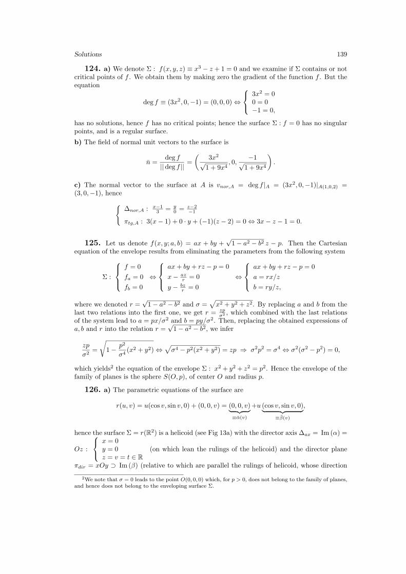
Solutions 139
124. a) We denote Σ : f(x, y, z) ≡ x3 − z + 1 = 0 and we examine if Σ contains or notcritical points of f . We obtain them by making zero the gradient of the function f . But theequation
deg f ≡ (3x2, 0,−1) = (0, 0, 0) ⇔
3x2 = 00 = 0−1 = 0,
has no solutions, hence f has no critical points; hence the surface Σ : f = 0 has no singularpoints, and is a regular surface.
b) The field of normal unit vectors to the surface is
n =deg f
||deg f ||=
(3x2√1 + 9x4
, 0,−1√
1 + 9x4
).
c) The normal vector to the surface at A is vnor,A = deg f |A = (3x2, 0,−1)|A(1,0,2) =(3, 0,−1), hence{
∆nor,A : x−13 = y
0 = z−2−1
πtg,A : 3(x− 1) + 0 · y + (−1)(z − 2) = 0 ⇔ 3x− z − 1 = 0.
125. Let us denote f(x, y; a, b) = ax + by +√1− a2 − b2 z − p. Then the Cartesian
equation of the envelope results from eliminating the parameters from the following system
Σ :
f = 0
fa = 0
fb = 0
⇔
ax+ by + rz − p = 0
x− azr = 0
y − bzr = 0
⇔
ax+ by + rz − p = 0
a = rx/z
b = ry/z,
where we denoted r =√1− a2 − b2 and σ =
√x2 + y2 + z2. By replacing a and b from the
last two relations into the first one, we get r = zpσ2 , which combined with the last relations
of the system lead to a = px/σ2 and b = py/σ2. Then, replacing the obtained expressions ofa, b and r into the relation r =
√1− a2 − b2, we infer
zp
σ2=
√1− p2
σ4(x2 + y2) ⇔
√σ4 − p2(x2 + y2) = zp ⇒ σ2p2 = σ4 ⇔ σ2(σ2 − p2) = 0,
which yields2 the equation of the envelope Σ : x2 + y2 + z2 = p2. Hence the envelope of thefamily of planes is the sphere S(O, p), of center O and radius p.
126. a) The parametric equations of the surface are
r(u, v) = u(cos v, sin v, 0) + (0, 0, v) = (0, 0, v)︸ ︷︷ ︸≡α(v)
+u (cos v, sin v, 0)︸ ︷︷ ︸≡β(v)
,
hence the surface Σ = r(R2) is a helicoid (see Fig 13a) with the director axis ∆ax = Im (α) =
Oz :
x = 0y = 0z = v = t ∈ R
(on which lean the rulings of the helicoid) and the director plane
πdir = xOy ⊃ Im (β) (relative to which are parallel the rulings of helicoid, whose direction
2We note that σ = 0 leads to the point O(0, 0, 0) which, for p > 0, does not belong to the family of planes,and hence does not belong to the enveloping surface Σ.
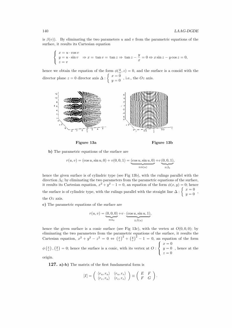
140 LAAG-DGDE
is β(v)). By eliminating the two parameters u and v from the parametric equations of thesurface, it results its Cartesian equation x = u · cos v
y = u · sin vz = v
⇒ x = tan v = tan z ⇒ tan z − y
x= 0 ⇔ x sin z − y cos z = 0,
hence we obtain the equation of the form ϕ( yx , z) = 0, and the surface is a conoid with the
director plane z = 0 director axis ∆ :
{x = 0y = 0
, i.e., the Oz axis.
Figure 13a Figure 13b
b) The parametric equations of the surface are
r(u, v) = (cosu, sinu, 0) + v(0, 0, 1) = (cosu, sinu, 0)︸ ︷︷ ︸≡α(u)
+v (0, 0, 1)︸ ︷︷ ︸≡β0
,
hence the given surface is of cylindric type (see Fig 13b), with the rulings parallel with thedirection β0; by eliminating the two parameters from the parametric equations of the surface,it results its Cartesian equation, x2 + y2 − 1 = 0, an equation of the form ϕ(x, y) = 0; hence
the surface is of cylindric type, with the rulings parallel with the straight line ∆ :
{x = 0y = 0
,
the Oz axis.
c) The parametric equations of the surface are
r(u, v) = (0, 0, 0)︸ ︷︷ ︸≡α0
+v · (cosu, sinu, 1)︸ ︷︷ ︸≡β(u)
,
hence the given surface is a conic surface (see Fig 13c), with the vertex at O(0, 0, 0); byeliminating the two parameters from the parametric equations of the surface, it results the
Cartesian equation, x2 + y2 − z2 = 0 ⇔(xz
)2+(yz
)2 − 1 = 0, an equation of the form
ϕ(xz
),(yz
)= 0; hence the surface is a conic, with its vertex at O :
x = 0y = 0z = 0
, hence at the
origin.
127. a)-b) The matrix of the first fundamental form is
[I] =
(⟨ru, ru⟩ ⟨ru, rv⟩⟨rv, ru⟩ ⟨rv, rv⟩
)≡(E FF G
).
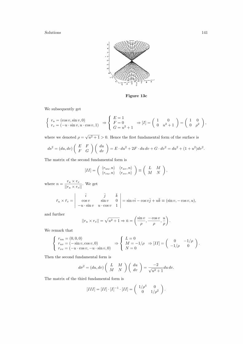
Solutions 141
Figure 13c
We subsequently get
{ru = (cos v, sin v, 0)rv = (−u · sin v, u · cos v, 1) ⇒
E = 1F = 0G = u2 + 1
⇒ [I] =
(1 00 u2 + 1
)=
(1 00 ρ2
),
where we denoted ρ =√u2 + 1 > 0. Hence the first fundamental form of the surface is
ds2 = (du, dv)
(E FF G
)(dudv
)= E · du2 + 2F · du dv +G · dv2 = du2 + (1 + u2)dv2.
The matrix of the second fundamental form is
[II] =
(⟨ruu, n⟩ ⟨ruv, n⟩⟨rvu, n⟩ ⟨rvv, n⟩
)≡(
L MM N
),
where n =ru × rv
||ru × rv||. We get
ru × rv =
∣∣∣∣∣∣i j k
cos v sin v 0−u · sin v u · cos v 1
∣∣∣∣∣∣ = sin vi− cos vj + uk ≡ (sin v,− cos v, u),
and further
||ru × rv|| =√u2 + 1 ⇒ n =
(sin v
ρ,− cos v
ρ,u
ρ
).
We remark that ruu = (0, 0, 0)ruv = (− sin v, cos v, 0)rvv = (−u · cos v,−u · sin v, 0)
⇒
L = 0M = −1/ρN = 0
⇒ [II] =
(0 −1/ρ
−1/ρ 0
).
Then the second fundamental form is
dσ2 = (du, dv)
(L MM N
)(dudv
)=
−2√u2 + 1
du dv.
The matrix of the third fundamental form is
[III] = [II] · [I]−1 · [II] =(
1/ρ4 00 1/ρ2
).
142 LAAG-DGDE
From the coefficients of the matrix of the first fundamental form we remark that
• ||ru||2 = ⟨ru, ru⟩ = E = 1, hence ||ru|| = 1 (ru is a unit vector);
• ||rv||2 = ⟨rv, rv⟩ = G = ρ2 = 0, hence ||ru|| ≥ 1 and rv is not generally a unit vector, and
• F = ⟨ru, rv⟩ = 0, hence ru ⊥ rv.
We conclude that rv not being unit vector at each point of the surface, the basis of the Gaussframe BG = {ru, rv, n} is not orthonormal.
c) The Gauss and mean curvatures of the surface are given by
K =det[II]
det[I], H =
1
2· EN + LG− 2FM
det[I],
and for the given surface we get,
K =−1/ρ2
ρ2= − 1
ρ4< 0, H =
1
2· 0 + 0 · 2
ρ2= 0.
d) Since K ≡ 0, the surface is not developable, but is minimal, since H ≡ 0. Since K < 0,it results that all the points of the surface are of hyperbolic type.
e) We check the Beltrami-Enneper formula, [III] − 2H[II] + K[I] = [0]. Indeed, we havethe identity(
1/ρ4 00 1/ρ2
)− 2 · 0 ·
(0 − 1
ρ
− 1ρ 0
)+
(− 1
ρ4
)(1 00 ρ2
)=
(0 00 0
).
128. a) The matrix of the Weingarten operator is given by the relation
[S] = [I]−1 · [II] =(
1 00 1/ρ2
)·(
0 −1/ρ−1/ρ 0
)=
(0 −1/ρ
−1/ρ3 0
).
b) According to the Rodriguez theorem, the principal curvatures k1,2 are exactly the eigen-values of the matrix [S], and the principal directions are given by a pair of eigenvectorsw1,2 associated to them. In order to find the eigenvalues of the matrix [S], we compute thecharacteristic polynomial,
P (λ) = det([S]− λI2) =
∣∣∣∣ −λ −1/ρ−1/ρ3 −λ
∣∣∣∣ = λ2 − 1
ρ4.
The characteristic equation is P (λ) = 0 and hence the roots are
λ1 = k1 = − 1
ρ2, λ2 = k2 =
1
ρ2.
We look for a pair of eigenvectors which correspond to the two eigenvalues.
For λ1 = − 1ρ2 , the characteristic system ([S]− λ1I2)w = 0 can be written, for w = (a, b)t,(
1ρ2 −1
ρ
− 1ρ3
1ρ2
)(ab
)=
(00
)⇔{b = s1ρ2 · a− 1
ρ · s = 0⇔{a = ρsb = s
⇒ (a, b) = s(ρ, 1);
The first principal direction is hence given by the tangent vector w1 = (ρ, 1),
w1 = (ρ, 1) ≡ ρru + rv ∈ Tr(u,v)Σ,
Solutions 143
whose components in the 3-dimensional space are
w1 ≡√1 + u2(cos v, sin v, 0) + 1 · (−u sin v, u cos v, 1).
For λ2 = 1ρ2 , the characteristic system ([S]− λ1I2)w = 0 can be written, for w = (a, b)t,(−1/ρ2 −1/ρ−1/ρ3 −1/ρ2
)(ab
)=
(00
)⇔{b = s− 1ρ2 · a− 1
ρ · s = 0⇔{a = −ρsb = s,
hence (a, b) = (−ρs, s) = s(−ρ, 1). The second principal direction is hence given by thevector
w2 = (−ρ, 1) ≡ −ρru + rv ∈ Tr(u,v)Σ,
whose components in the 3-dimensional space are
w2 ≡ −√
1 + u2(cos v, sin v, 0) + 1 · (−u sin v, u cos v, 1).
We can determine the two principal curvatures k1,2 by using the curvatures K and H of thesurface. These satisfy the equation
λ2 − 2Hλ+K = 0 ⇔ λ2 − 1
ρ4= 0 ⇒
{k1 = − 1
ρ2
k2 = 1ρ2 .
c) The tangent vector w = 2ru − rv ≡ (2,−1) has its associated normal curvature:
kn(w) =[II](w,w)
[I](w,w)=
(2,−1)
(0 − 1
ρ
− 1ρ 0
)(2−1
)(2,−1)
(1 00 ρ2
)(2−1
) =
4ρ
4 + ρ2=
4
ρ(4 + ρ2).
We find the values of the parameters u and v which correspond to the point A(−1, 0, π), bysolving the system u · cos v = −1
u · sin v = 0v = π
⇒{u = 1v = π
⇔ (u, v) = (1, π),
from where ρ|A =√2, and kn(w) =
4√2(4+2)
= 23√2=
√23 . Moreover, the effective direction
(in 3D) determined by w is given by
w = (2ru − rv)|A ≡ 2(−1, 0, 0)− (0,−1, 1) = (−2, 1,−1).
d) We remark that in item A we have ρ =√2, hence k1 = −1
2 , k2 = 12 . Then, relative to a
conveniently chosen coordinate system, the surface has the form similar to the one describedby the Cartesian equation
Σaprox : z =1
2
(−1
2x2 +
1
2y2)
⇔ y2
4− x2
4= z,
hence locally, the surface has the form of a hyperbolic paraboloid (see Fig 14).
129. We check the Meusnier Theorem, which states:
Let α = r ◦ (u, v) : I ⊂ R → R3 be a curve on the surface Σ = Im r. Then
kn(α′) = kα · cos θ, (41)
where:
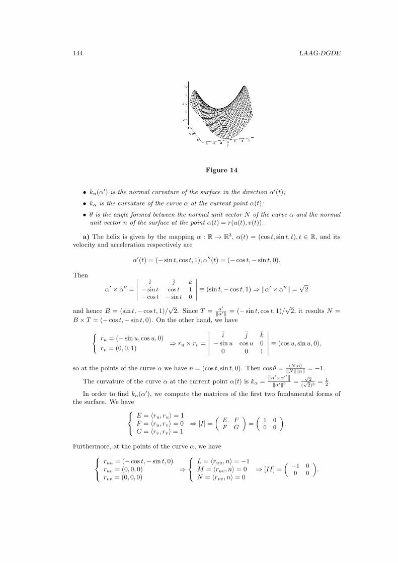
144 LAAG-DGDE
Figure 14
• kn(α′) is the normal curvature of the surface in the direction α′(t);
• kα is the curvature of the curve α at the current point α(t);
• θ is the angle formed between the normal unit vector N of the curve α and the normalunit vector n of the surface at the point α(t) = r(u(t), v(t)).
a) The helix is given by the mapping α : R → R3, α(t) = (cos t, sin t, t), t ∈ R, and itsvelocity and acceleration respectively are
α′(t) = (− sin t, cos t, 1), α′′(t) = (− cos t,− sin t, 0).
Then
α′ × α′′ =
∣∣∣∣∣∣i j k
− sin t cos t 1− cos t − sin t 0
∣∣∣∣∣∣ ≡ (sin t,− cos t, 1) ⇒ ∥α′ × α′′∥ =√2
and hence B = (sin t,− cos t, 1)/√2. Since T = α′
∥α′∥ = (− sin t, cos t, 1)/√2, it results N =
B × T = (− cos t,− sin t, 0). On the other hand, we have{ru = (− sinu, cosu, 0)
rv = (0, 0, 1)⇒ ru × rv =
∣∣∣∣∣∣i j k
− sinu cosu 00 0 1
∣∣∣∣∣∣ ≡ (cosu, sinu, 0),
so at the points of the curve α we have n = (cos t, sin t, 0). Then cos θ = ⟨N,n⟩∥N∥∥n∥ = −1.
The curvature of the curve α at the current point α(t) is kα =∥α′×α′′∥
∥α′∥3 =√2
(√2)3
= 12 .
In order to find kn(α′), we compute the matrices of the first two fundamental forms of
the surface. We have E = ⟨ru, ru⟩ = 1F = ⟨ru, rv⟩ = 0G = ⟨rv, rv⟩ = 1
⇒ [I] =
(E FF G
)=
(1 00 0
).
Furthermore, at the points of the curve α, we have ruu = (− cos t,− sin t, 0)ruv = (0, 0, 0)rvv = (0, 0, 0)
⇒
L = ⟨ruu, n⟩ = −1M = ⟨ruv, n⟩ = 0N = ⟨rvv, n⟩ = 0
⇒ [II] =
(−1 00 0
).
Solutions 145
Also, relative to the basis B = {ru, rv} of the tangent space Tα(t)Σ to the surface at α(t),we have
α′(t) = u′(t) · ru|α(t) + v′(t) · rv|α(t) = 1 · ru|α(t) + 1 · rv|α(t),
and hence v[α′]B = (1, 1)t, and therefore
kn(α′) =
vt[II]v
vt[I]v=
(1, 1)
(−1 00 0
)(11
)(1, 1)
(1 00 1
)(11
) = −1
2.
Then formula (41) becomes − 12 = 1
2 · (−1), which is an identity at each point of the curve α.
b) The equality z = x becomes, on α, v = cosu, which suggests the parameterization{u(t) = tv(t) = cos t,
, and hence α(t) = r(u(t), v(t)) = (cos t, sin t, cos t). We notice that the
rotation R of angle −π/4 and Oy as axis of rotation, transforms the curve α into γ = R ◦α,
γ(t) =
cosπ/4 0 sinπ/40 1 0
− sinπ/4 0 cosπ/4
cos t
sin tcos t
=
2 cos t/√2
sin t0
,
and therefore the Cartesian coordinates of the points located on the curve γ satisfy the
equations Im γ :
{x2
2 + y2 = 1z = 0
, an ellipse, and hence α = R−1 ◦ γ is an ellipse as well.
In order to compute N and kα, we first compute:{α′(t) = (− sin t, cos t,− sin t)
α′′(t) = (− cos t,− sin t,− cos t)⇒ α′ × α′′ = (−1, 0, 1) ⇒ B = (−1, 0, 1)/
√2
and since T = (− sin t, cos t,− sin t)/√1 + sin2 t, we infer kα =
∥α′×α′′∥∥α′∥3 =
√2
(1+sin2 t)3/2and
N = B × T = (− cos t,−2 sin t,− cos t)/
√2(1 + sin2 t).
Further, according to item a), on the curve α we have n = (cos t, sin t, 0), and hence
cos θ =⟨n,N⟩
∥n∥ · ∥N∥=
−(1 + sin2 t)√2(1 + sin2 t)
= −√1 + sin2 t√
2.
Also, α′(t) = u′(t)ru|α(t) + v′(t)rv|α(t) = 1 · ru|α(t) + 1 · rv|α(t), and hence v = [α′]β =(1,− sin t)t, and consequently
kn(α′) =
(1,− sin t)
(−1 00 0
)(1
− sin t
)(1,− sin t)
(1 00 0
)(1
− sin t
) =−1
1 + sin2 t.
Then the equality (41) becomes
−1
1 + sin2 t=
√2
(1 + sin2 t)3/2·
(−√1 + sin2 t√
2
),
which is an identity along the curve α.
146 LAAG-DGDE
130. We apply the Euler Theorem, which states:
Let v ∈ TpΣ be a tangent vector to the surface Σ and we denote by θ the oriented angle θ =^(e1, v), where {e1, e2} are the principal unit vectors respectively associated to the principalcurvatures k1 and k2. Then
kn(v) = k1 cos2 θ + k2 sin
2 θ. (42)
a) From the previous exercise, we have v = [α′]B = (1, 1)t, kn(v) =12 . The matrix of the
Weingarten operator relative to the tangent basis {ru, rv} is
[S] = [I]−1
[II] =
(−1 00 0
)and its eigenvectors are {e1 = (1, 0)t, e2 = (0, 1)t}, respectively associated to the eigenvalues
k1 = −1, k2 = 0. We have cos θ = ⟨e1,v⟩∥e1∥∥v∥ -where the angles are computed using the matrix
of the induced scalar product, [I] = I2, and hence cos θ = 1√2. Then the relation (42) can be
written as
−1
2= (−1) ·
(1√2
)2
+ 0 ·(± 1√
2
)2
,
hence we get an identity.
b) We have v = [α′]B = (1,− sin t), kn(v) =−1
1+sin2 tand cos θ = 1√
1+sin2 t, sin θ = ± sin t√
1+sin2 t.
Then the equality (42) has the form
−1
1 + sin2 t= (−1) ·
(1√
1 + sin2 t
)2
+ 0 ·
(± sin t√1 + sin2 t
)2
,
which is an identity.
131. a) We parametrize the curve, by denoting u = t; it results v = 2t, hence
α(t) = r(t, 2t) = (t cos 2t, t sin 2t, 2t), t ∈ [1, 2],
andα′(t) = (cos 2t− 2t sin 2t, sin 2t+ 2t cos 2t, 2) ⇒ ||α′(t)|| =
√4t2 + 1 + 4.
Then, using a replacement of Euler type for computing the definite integral, the arc-lengthof the curve follows:
l =
∫ 2
1
||α′(t)||dt =∫ 2
1
√4t2 + 5dt =
√21− 15
8· ln 5 + 5
4· ln(4
√5 +
√21
√5)− 3
2.
b) We apply the area formula
A =
∫∫D
√det[I] du dv =
∫∫D
√EG− F 2 du dv =
=
∫∫D
√1(1 + u2)− 02du dv =
∫ 1
0
du
∫ π
0
√1 + u2dv =
=∫ 1
0
√1 + u2du ·
∫ π0dv = π ·
∫ 1
0
√1 + u2du.
Using the substitution√u2 + 1 = u+ t it results
u2 + 1 = u2 + 2tu+ t2 ⇒ u = 1−t22t
du = 12 · −2t2−(1−t2)
t2 dt = −1+t2
2t2 dt√u2 + 1 = u+ t = 1−t2
2t + t = 1+t2
2t .
Solutions 147
As well, we have u = 0 ⇒ t = 1 and u = 1 ⇒ t =√2− 1, hence
A = π
∫ √2−1
1
1 + t2
2t· (−1 + t2
2t2)dt =
π
4
∫ 1
√2−1
(1 + t2)2
t3dt =
π
4
∫ 1
√2−1
(t2 +2
t+
1
t3)dt =
= π4 · ( t
2
2 + 2 ln |t|+ t−2
−2 )|1√2−1
= π4
[( 12 + 2 ln 1− 1
2 )− ( 3−2√2
2 + 2 ln(√2− 1) + 1
2(3−2√2))]
= π4 · 1
2
[3− 2
√2 + 4 ln(
√2− 1) + 1
2(3−2√2
]= π
8 (3− 2√2 + 4 ln(
√2− 1) + 3 + 2
√2) =
= π8 · 6 + π
8 · 4 ln(√2− 1) = 3π
4 + π2 ln(
√2− 1).
132. a) The differential equation of the curvature lines α(t) = r(u(t), v(t)) is∣∣∣∣∣∣v′2 −u′v′ u′2
E F GL M N
∣∣∣∣∣∣ = 0.
We compute the coefficients of the lower lines of the determinant,{ru = (− sinu, cosu, 0)rv = (0, 0, 1)
⇒
E = ⟨ru, ru⟩ = 1F = ⟨ru, rv⟩ = 0G = ⟨rv, rv⟩ = 1.
We get ruu = (− cosu,− sinu, 0)ruv = (0, 0, 0)rvv = (0, 0, 0)
⇒
L = ⟨ruu, n⟩ = −1M = ⟨ruv, n⟩ = 0N = ⟨rvv, n⟩ = 0.
We find the field n of unit vectors normal to the surface,
ru × rv =
∣∣∣∣∣∣i j k
− sinu cosu 00 0 1
∣∣∣∣∣∣ ≡ (cosu, sinu, 0) ⇒ ||ru × rv|| =√1 = 1,
hence n = (cosu, sinu, 0). Then the differential equation of the lines of the curvature (theequation of the principal curves) becomes∣∣∣∣∣∣
v′2 −u′v′ u′2
1 0 1−1 0 0
∣∣∣∣∣∣ = 0 ⇔ u′v′ = 0.
The following cases appear:
Case I. u′ = 0 ⇔ u(t) = a = const.. We denote v(t) = t and we get the curves
α(t) = r(a, t) = (cos a, sin a, t), t ∈ R.
We obtain their Cartesian equations by eliminating the parameter t from the parametricequations, x = cos a
y = sin az = t
⇒{
x− cos a = 0 (plane)y − sin a = 0 (plane),
hence each of the curves is a straight line. We see this, by noticing that the parametric
equations of these curves are of the form
x = 0t+ cos ay = 0t+ sin az = 1t+ 0, t ∈ R
from which, by eliminating
the parameter t, we infer the canonic Cartesian equations of a family of straight lines
(t =)x− cos a
0=y − sin a
0=z − 0
1
148 LAAG-DGDE
whose direction is v = (0, 0, 1) ≡ k, hence these are straight lines parallel with the Ozaxis. These are exact the rulings of the given cylinder. We remark, indeed, that the givenparametrized surface is a cylinder, since its Cartesian equation, obtained from the parametricequations, x = cosu
y = sinuz = v
⇒ x2 + y2 = 1,
is the equation of a right circular cylinder whose radius is 1 and whose axis of symmetry isOz. We conclude that the first family of principal curves of the given cylinder consists of itsrulings.
Case II. v′ = 0 ⇒ v(t) = b = const.. By denoting u = t, we get the parametric equation andthen, the Cartesian ones of the second family of principal curves,
β(t) = r(t, b) = (cos t, sin t, b) ⇔
x = cos ty = sin tz = b.
By eliminating the parameter t, we infer the Cartesian equations of these curves,{x2 + y2 = 1 (the given cylinder Im r)z − b = 0 (plane perpendicular to the axis of Im r)
and hence the principal curves of the second family are section circles of the cylinder. Weconclude that the principal curves of the cylinder consist of rulings and circles.
b) The asymptotic curves (”asymptotic lines”) satisfy the differential equation
(u′, v′)[II]
(u′
v′
)= 0.
By replacing L,M,N determined in item a), we get the matrix [II] =
(−1 00 0
), hence
the equation of asymptotic lines becomes
(u′, v′)
(−1 00 0
)(u′
v′
)= 0 ⇔ −u′2 = 0 ⇔ u′ = 0.
But u′ = 0 ⇒ u(t) = a = const. and v(t) = t, hence we get the rulings of the cylinderconsidered in the previous item. We conclude that the asymptotic lines of the cylinder areits rulings.
c) We find the geodesics of the cylinder. In order to obtain the equations of geodesicsα(t) = r(u(t), v(t)), we impose the conditions that these have unit speed (||α′(t)|| = 1) andto satisfy the relation α′′(t) ⊥ Tα(t)Σ. All in all, these conditions have the form ⟨α′′, ru|α(t)⟩ = 0
⟨α′′, rv|α(t)⟩ = 0⟨α′, α′⟩ = 1,
We subsequently get{α′ = u′ru + v′rvα′′ = u′′ru + v′′rv + u′2ruu + 2u′v′ruv + v′2rvv.
In our case, r(u, v) = (cosu, sinu, v) and we get
α′ = u′(− sinu, cosu, 0) + v′(0, 0, 1).
Solutions 149
By replacing in the three relations of the previous system, we inferu′′E + v′′F + u′2⟨ruu, ru⟩+ 2u′v′⟨ruv, ru⟩+ v′2⟨rvv, ru⟩ = 0
u′′F + v′′G+ u′2⟨ruu, rv⟩+ 2u′v′⟨ruv, rv⟩+ v′2⟨rvv, rv⟩ = 0
Eu′2 + 2Fu′v′ +Gv′2 = 1.
By replacing the partial derivatives, it resultsu′′ · 1 + v′′ · 0 + u′2 · 0 + 2u′v′ · 0 + v′2 · 0 = 0
u′′ · 0 + v′′ · 1 + u′2 · 0 + 2u′v′ · 0 + v′2 · 0 = 0
1 · u′2 + 2 · 0 · u′v′ + 1 · v′2 = 1,
from where it results u′′ = 0 ⇒ u′ = a ⇒ u = at+ b
v′′ = 0 ⇒ v′ = c ⇒ v = ct+ d
u′2 + v′2 = 1 ⇒ a2 + c2 = 1.
(43)
We find the curve α by substituting the obtained functions u and v in the parametric equationof the surface,
α(t) = r(u(t), v(t)) = (cos(at+ b), sin(at+ b), ct+ d).
We examine the curve α; we have three cases:
i) a = 0; from the third relation (43), it results c = ±1, hence we get the curves
α1(t) = (cos b, sin b,±t+ d);
by eliminating the parameter t from the obtained parametric equations, it results that theseare the rulings of the cylinder, which are parallel with the Oz axis and are located at distance1 relative to the axis,
∆ :x− cos b
0=y − sin b
a=z − d
±1(= t).
ii) c = 0; from the third relation (43), it results a = ±1; hence, we get
α2(t) = (cos(±t+ b), sin(±t+ b), d).
By eliminating the parameter t, we notice that we obtain a family of circles of Cartesianequations {
x2 + y2 = 1
z = d.
We conclude that the second family of geodesics of the cylinder consists of transversal sec-tional circles.
iii) If a = 0, c = 0 and a2 + c2 = 1, then
α3(t) = (cos(at+ b), sin(at+ b), ct+ d).
By performing the change of parameter θ = at+b, it results t = θ−ba and ct+d = cθ
a − bca +d =
mθ + n, where we denoted m = ca , n = − bc
a + d. Then, re-parametrizing the curve α3, weget its new equation
α3(θ) = (cos θ, sin θ,mθ + n).
150 LAAG-DGDE
We remark that we obtain a family of helices. We conclude that the geodesics of the cylinderare
• straight lines (the rulings of the cylinder),• circles (obtained by cutting the cylinder with planes transversal on its symmetry axis),• helices.
V.1. Ordinary differential equations
133. By deriving the given relations, it results
y′ cos y − c = 0 ⇒ c = y′ cos y.
By replacing the obtained value for c in the relation, it results
sin y − y′ cos y · x = 0 ⇔ xy′ cos y − sin y = 0,
the given equation, which proves that the implicitly given function y satisfies the equation.
Otherwise. Using the given relation, we explicitly write the function y,
sin y − cx = 0 ⇒ sin y = cx⇒ y = kπ + (−1)k arcsin(cx) ⇒ y′ = (−1)kc√1−c2x2
,
and sin y = sin(kπ + (−1)k arcsin(cx)) = cx,
cos y = cos(kπ + (−1)k arcsin cx) = (−1)k ·√
1− sin2(arcsin cx) = (−1)k√1− c2x2.
By replacing y′, sin y and cos y in the equation, this becomes
xy′ cos y − sin y = 0 ⇔ x · (−1)kc√1− c2x2
· (−1)k√1− c2x2 − cx⇔ 0 = 0,
identity; hence the function y is the solution of the given differential equation.
134. We replace y′ = dydx in the equation and we get
x · dydx
· cos y = sin y ⇔ cos y
sin y· dy =
dx
x
from where, by integrating the two members of the equality, it results∫cos y
sin ydy =
∫dx
x⇔ ln | sin y| = ln |x|+ c0, c0 ∈ R.
By denoting c0 = ln |c1|, we get
ln | sin y| = ln |c1x| ⇒ sin y = ±c1x⇒ sin y − cx = 0,
where c = ±c1; we have the explicitly given solution y = kπ + (−1)k arcsin(cx), k ∈ ZZ.
135. a) In case of homogeneous equations, the derivative depends only on the ratio yx ,
hence these equations are of the form y′ = f( yx ).
The given equation can be written as y′ = y2
x2 , hence it is a homogeneous differential equation.We apply the integration algorithm for such type of equations, by performing the change of
unknown function y → u(x) = y(x)x given by the relations y = u · x ⇔ u = y
x . We have
Solutions 151
y = u · x ⇒ y′ = u′ · x+ u. By replacing in the equation we get u′x+ u = u2, the equationwith separable variabile . By substituting u′ = du
dx , it results
du
dx· x = u2 − u⇔ du
u2 − u=dx
x⇔ du
u(u− 1)=dx
x,
the equation with separate variables. By integration in its both sides, it results F (u) = ln |x|,where we denoted F (u) =
∫du
u2−u = ln |u−1u | + c1. By denoting c1 = − ln |c0| (c0 = 0) and
considering that u = y/x, we get
ln
∣∣∣∣u− 1
u
∣∣∣∣− ln |c0| = ln |x| ⇔ c0x =u− 1
u⇔ y =
x
1− c0x, c0 = 0.
But for c0 = 0 we get a solution as well, y = x, hence by extending by continuity for theparameter c0 the family of solutions and denoting c = −c0, it results the general solution ofthe equation,
y =x
1 + cx, c ∈ R.
b) The given equation can be written
y′ =sin y
x
cos yx⇔ y′ = tan
y
x,
hence it is a homogeneous differential equation. We apply the integration algorithm of such
equations, by performing the change of unknown function y 7→ u(x) = y(x)x given by the
relations y = u · x⇔ u = yx . We have
y = u · x⇒ y′ = u′x+ u.
By replacing in the equation we get u′x + u = tanu, an equation with separable variables.By substituting u′ = du
dx , it results
du
dx· x = tanu− u⇔ du
tanu− u=dx
x,
the equation with separate variables; by integrating its both sides, it results F (u) = ln |x|+ln |c0|, where we denoted F (u) =
∫du
tanu−u . By denoting c = ±c0, it results
F (u)− ln |c0x| = 0 ⇔ c0x = ±eF (u) ⇔ cx = eF (u),
and using u = yx , we have
cx = eF (y/x) ⇔ cx− eF (y/x) = 0,
hence we obtain the solution y(x) of the equation in implicit form.
136. a) The given equation, (x+ y− 1)dx+ (x− y− 1)dy = 0, is obviously of the form:
(a1x+ b1y + c1)dx+ (a2x+ b2y + c2)dy = 0, (44)
where a21 + b21 > 0, a22 + b22 > 0. We perform the double change of variable and unknownfunction x→ X; y(x) → Y (X) given by the relations{
X = x− x0Y = y − y0
⇔{x = X + x0y = Y + y0,
152 LAAG-DGDE
where (x0, y0) are the solutions of the system given by the intersection of the straight lines∆1 and ∆2, {
∆1 : x+ y − 1 = 0∆2 : x− y − 1 = 0
⇔{x0 = 1y0 = 0.
We practically perform the translation of frame xOy 7→ XO′Y (where O′(x0, y0)), given by{x = X + 1y = Y + 0.
(45)
By differentiation, we get
{dx = dXdy = dY.
By replacing in the equation, this becomes (X +
Y )dX + (X − Y )dY = 0. Dividing the equation by dX and by replacing Y ′ = dYdX , we get
(X + Y ) + (X − Y )Y ′ = 0 ⇔ Y ′ =Y +X
Y −X⇔ Y ′ =
YX + 1YX − 1
,
where the expression from the right hand side depends only on the ratioY
X, hence we obtain
a homogeneous equation. We substitute
u =Y
X⇔ Y = uX, (46)
from where, by derivation, it results Y ′ = u′X+u. By replacing in the equation, this becomesu′X + u = u+1
u−1 .
Denoting u′ = dudX , we get
du
dX·X =
1 + 2u− u2
u− 1⇔ (u− 1)du
1 + 2u− u2=dX
X,
from where, by the integration of the obtained equation with separate variables, it results∫u− 1
1 + 2u− u2du = ln |cX| ⇔ F (u)− ln|cX| = 0,
where we denoted F (u) =∫
u−11+2u−u2 du. We get back to the function Y (X); using the
relation (46), we get F ( YX )− ln |c(x− 1)| = 0. Then, using (45), we have
{X = x− 1Y = y
and
we obtain the solution in implicit form of the given differential equation,
F
(y
x− 1
)− ln |c(x− 1)| = 0.
b) (x + y − 1)dx + (x + y)dy = 0 is obviously an equation of type (44). Since the system{∆1 : x+ y − 1 = 0∆2 : x+ y = 0
is incompatible, we perform the change of unknown function y(x) 7→
u(x) = x+ y(x), given by the relation
u = x+ y ⇔ y = u− x, (47)
from where by differentiation, it results dy = du − dx. By replacing in the given equation,we get
(u− 1)dx+ u(du− dx) = 0 ⇔ (u− 1)dx+ udu− udx = 0 ⇔ udu− dx = 0 ⇔ udu = dx,
Solutions 153
an equation with separate variables; by integration, it results u2
2 = x+C. Using the substi-tution (47) it results the solution given by the Cartesian implicit equation
(x+ y)2
2= x+ C. (48)
Check. By isolating the constant C, the equation (48) can be written as (x+y)2
2 −x = C. Wedifferentiate the equality in both its sides and we yield(
2(x+ y)
2− 1
)dx+
2(x+ y)
2dy = 0 ⇔ (x+ y − 1)dx+ (x+ y)dy = 0,
hence the initial equation, which proves that the solution is correct.
137. a) We find both the general solution of the equation, and the solution whichsatisfies the condition which is indicated in the statement of the problem (y(1) = 1). Theequation and the initial condition form together a Cauchy problem, and the solution of thisproblem is unique and is called the solution of the Cauchy problem. At item b) we shalldetermine the general solution of the equation.
We first find the general solution of the differential equation; we notice that this is the lineardifferential equation of first order, i.e., of the form
y′ = f(x) · y + g(x). (49)
Indeed, by dividing the equation to x, we get y′ = (−2x )y + 3, hence the linear differential
equation with f(x) = −2x , g(x) = 3. The algorithm for solving a linear equation has three
steps:
1) We find the solution yom of the associated homogeneous equation y′ = f(x)y;2) We find a solution yp of the initial equation y′ = f(x)y + g(x) using the constant
variation method;3) The general solution is y = yom + yp.
We follow the three steps of the integration process.
1) The given equation is y′ = (− 2x )y + 3, hence the associated homogeneous equation is the
equation with separable variables
y′ = − 2
xy ⇔ dy
dx=
−2y
x⇔ dy
y= −2
dx
x,
from where, by denoting c = ±c0, integration leads to∫dy
y= −2
∫dx
x⇔ ln |y| = −2 ln |x|+ ln |c0| ⇒ |y| =
∣∣∣ c0x2
∣∣∣⇔ y =±c0x2
⇔ y =c
x2.
Check. If y = cx2 , then y
′ = −−2cx3 and hence, by replacing c = x2y in the derivative, we get
y′ =
(− 2
x
)y ⇔ −2c
x3= − 2
x· cx2,
which is a valid equality. Hence the solution of the associated homogeneous equation isyom = c
x2 .
2) We apply the constant variation method, to obtain a particular solution yp of the initialequation y′ = − 2
xy+3. By replacing in yom, the constant c with a function c(x), we determine
a function c(x), such that yp = c(x)x2 to be the solution the initial equation. By derivation,
154 LAAG-DGDE
we get yp′ = c′(x)·x2−2xc(x)
x4 . By replacing yp and yp′ in the equation, we put the condition
for the equation to be satisfied, which leads to
c′(x)
x2− 2c(x)
x3= −2c(x)
x3+ 3 ⇔ c′(x) = 3x2,
from where by integration we get c = x3 and hence yp =c(x)x2 = x3
x2 = x.
Check. We replace yp = x in the given equation, y′ = − 2x · y + 3. We get the valid equality
1 = − 2x · x+ 3.
3) We conclude that the general solution of the linear equation is
y = yom + yp =c
x2+ x.
where c ∈ R. We find the solution of the Cauchy problem
{y′ = − 2
xy + 3y(1) = 1
. From all the
solutions y = cx2 + x, we select the one which satisfies the condition y(1) = 1; by replacing
y in this relation, we get 1 = c12 + 1, hence c = 0; we infer that the solution of the Cauchy
problem is y = 0x2 + x, i.e., y = x.
b) We have the equation
xy′ + 3y = x2 ⇔ y′ = (− 3
x)y + x,
hence the differential equation is linear, of the form (49), with f(x) = − 3x and g(x) = x. We
perform the three integration steps.
1) The given equation is y′ = (− 3x )y + x, hence the associated homogeneous equation is the
equation with separable variables
y′ = − 3
xy. (50)
By denoting y′ = dydx , this can be subsequently written:
dy
dx= −3y
x⇔ dy
y= −3
dx
x,
from where, by integration, it results (here c = ±c0):∫dy
y= −3
∫dx
x⇔ ln |y| = −3 ln |x|+ ln |c0| ⇒
⇒ |y| = | c0x3
| ⇔ y = ± c0x3
⇔ y =c
x3.
Homework. Show that y satisfies the differential homogeneous equation (50).
2) We apply the constant variation method to obtain a particular solution yp of the initialequation y′ = (− 3
x )y+ x. We replace in yom the constant c with a function c(x) and we put
the condition that yp =c(x)x3 to be the solution of the initial equation. By derivation, we get
y′p =c′(x) · x− c(x) · 3
x4
By replacing yp and y′p in the equation, we put the condition that the equation be satisfied,from where it results
c′(x)
x3− 3c(x)
x4= −3c(x)
x4+ x⇔ c′(x) = x4,
Solutions 155
from where, by integration (by considering a particular integration constant, e.g., null), we
get c = x5
5 and hence yp =c(x)x3 = x5
5x3 = x2
5 .
3) We conclude that the general solution of the linear equation is y = yom + yp = cx3 + x2
5 ,where c ∈ R.
138. a) The equation can be written y′ = y · 1+ y1/2(−x), hence it is of Bernoulli type,being of the form
y′ = y · f(x) + yrg(x), r ∈ R\{0, 1}. (51)
We perform the change of unknown function which is specific to this type of equation,y(x) 7→ z(x) = (y(x))1−r, given by the relation z = y1−r. In our case, z = y1/2 ⇒ y = z2,from where by derivation it results y′ = 2z · z′. By replacing in the given equation, we get2zz′ = z2 − xz. We have two cases:
Case I. z = 0 ⇒ y = z2 = 0 ⇒ y = 0, a singular solution of the equation; check: 0 = 0−x·√0,
identity.
Case II. z = 0. We have
2z′ = z − x⇔ z′ =1
2z +
(−x2
).
We obtained a linear equation in the unknown function z. We apply the three steps in solvingthe linear differential equation:
1) By denoting c = ±ec1 , it results
z′ =z
2⇒ z′
z=
1
2⇔ ln |z| = x
2+ c1 ⇔ |z| = ec1 · ex/2 ⇔ z = c · ex/2,
hence we get the solution zom = c · ex/2.2) We apply the constant variation method: we look for a solution zp of the form zp =c(x) · ex/2; by introducing in the original equation, we get
c′ · ex/2 + 1
2c · ex/2 =
1
2c · ex/2 − x
2⇔ c′ = −x
2· e−x/2,
from where, by integration, we get
c = −12
∫x · e−x/2dx⇒ c = −1
2
∫x(e−x/2)′ · (−2)dx =
= x · e−x/2 −∫e−x/2dx = x · e−x/2 + 2e−x/2 = (x+ 2) · e−x/2,
hence zp = (x+ 2) · e−x/2︸ ︷︷ ︸c(x)
) · e−x/2 = x+ 2.
3) The solution of the linear differential equation is hence z = zom + zp = c · ex/2 + x + 2,hence y = z2 = (c · ex/2 + x+ 2)2.
b)By replacing dydx = y′, the equation can be written y′ = y · x + y3 · (−x), hence the
equation is of Bernoulli form (51), with r = 3. We perform the substitution z = y1−s, hence
z = 1y2 ⇒ y = z−1/2, from where, by derivation, it results y′ = − z′
2√z3. By replacing in the
given equation, we get
− z′
2√z3
=1√z· x− 1√
z3· x⇔ z′ = −2zx+ 2x.
We obtained the equation linear in the unknown function z. We proceed as in item a):
156 LAAG-DGDE
1) The associated homogeneous equation can be written:
z′ = −2zx⇒ z′
z= −2x⇔ ln |z| = −x2 + c1 ⇔
⇔ |z| = ec1 · e−x2
⇔ z = c · e−x2
,
where we denoted c = ± · ec1 , hence we get the solution zom = c · e−x2
.
2) By applying the constant variation method, we look for a solution zp of the form zp =
c(x) · e−x2
; by introducing in the original equation, we get
c′ · e−x2
+ (−2x) · c · e−x2
= −2x · c · e−x2
+ 2x⇔ c′ = 2x · ex2
,
from where, by integration we have c = 2∫x · ex2
dx = ex2
and hence zp = ex2 · e−x2
= 1.
3) The solution of the linear differential equation is hence z = zom + zp = c · e−x2
+1, whichleads to y = 1√
z= 1√
c·e−x2+1.
139. a) Since we know the form of the particular solution of the equation, for findingthe constant a, we impose that y1 to satisfy the given equation; we have y1 = 1
x+a ⇒ y′1 =
− 1(x+a)2 . By replacing y1 and y′1 in the equation, we get
− 1
(x+ a)2=
x
(x+ a)2− 1
x+ a⇔ a = 1 ⇒ y1 =
1
x+ 1.
The given equation can be written
y′ = y2 · x+ y · (−1) + 0,
and it is of Riccati type, being of the form
y′ = y2 · f(x) + y · g(x) + h(x).
We perform the change of unknown function which is specific to this type of equation,y(x) 7→ z(x) = 1
y(x)−y1 , given by the relation y = y1 +1z . In our case we have
y =1
x+ 1+
1
z, (52)
from where by derivation it results y′ = − 1(x+1)2 − 1
z2 · z′. By replacing y and y′ in theequation, we get
− 1
(x+ 2)2− z′
z2=
x
(x+ 1)2+
2x
z(x+ 1)+
x
z2− 1
x+ 1− 1
z.
The equation can be written as − z′
z2 = x+1(x+1)2 − 1
x+1 + 2xz(x+1) +
xz2 − 1
z and grouping with
common denominator leads to the following linear equation in the unknown z:
z′ = z · 1− x
1 + x+ x.
Homework. Find the general solution z(x, c) = ce−x(x + 1)2 + x + 1, c ∈ R of the equationand then, using (52) deduce the solution of the initial equation, y = 1
x+1 + 1z(x,c) = 1
x+1 +
(ce−x(x+ 1)2 + x+ 1)−1.
Solutions 157
b) The given equation can be written as y′ = y2 · (−1)+ y · 0+ 2x2 , hence it is an equation of
Riccati type. In order to find the constant a, we impose that y1 to satisfy the given equation;we have y1 = a
x ⇒ y′1 = − ax2 . By replacing y1 and y′1 in the equation, we get
− a
x2+a2
x2=
2
x2⇔ a2 − a− 2 = 0 ⇒ a1 = −1 sau a2 = 2.
In the following we address the case a = −1. We perform the change of unknown functionz = 1
y−y1 , from where y = y1 +1z . In our case we get
y = − 1
x+
1
z. (53)
from where, by derivation, it results y′ = 1x2 − 1
z2 · z′. By replacing y and y′ in the equation,we get
1
x2− z′
z2= − 1
x2+
2
xz− 1
z2+
2
x2⇔ z′ = −2
z
x+ 1
The equation is of the form z′ = f( zx ), hence it is homogeneous. We change the unknown
function z → t = t(x) with t = zx , and it results dy
dx = t+ x · dtdx ; by replacing in the equation
we have : t + x dtdx = −2t + 1, i.e., dt−3t+1 = dx
x , the equation with separate variables. By
integration we get − 13 ln |−3t+ 1| = ln |x|+ln |c| , c = 0, i.e., t = 1
3 (1−1
(cx)3 ). By replacing
t = zx , it results z =
x3 (1−
1(cx)3 ).
140. a) The equation is of the form P dx+Qdy = 0 and satisfies the exactness condition
∂P
∂y=∂Q
∂x.
Indeed, the equation can be written, by amplifying with dx and using the substitutiony′ = dy
dx ,
(x+ y)︸ ︷︷ ︸P
dx+ (x+ 2y)︸ ︷︷ ︸Q
dy = 0,
We have ∂P∂y = 1; ∂Q
∂x = 1, hence the given equation differential is exact. We get the solutionof the equation in implicit form, by applying the formula∫ x
x0
P (u, y)du+
∫ y
y0
Q(x0, v)dv = c, c ∈ R,
and hence,
∫ xx0(u+ y)du+
∫ yy0(x0 + 2v)dv = c⇔ u2
2
∣∣∣∣xx0
+ uy|xx0+ x0v
∣∣∣∣yy0
+ v2∣∣∣∣y=yy=y0
= c⇔
⇔ x2−x20
2 + y(x− x0) + x0(y − y0) + y2 − y20 = c;
choosing x0 = 0 and y0 = 0, it results the solution in implicit Cartesian form:
x2
2+ xy + y2 = c. (54)
Check. In order to test the solution, we differentiate the relation (54) and we get
(x+ y) · dx+ (x+ 2y) · dy = 0,
158 LAAG-DGDE
which is equivalent with the initial equation, and hence the solution satisfies the given equa-tion.
b) We have the equation (x2 + y2 + 2x)︸ ︷︷ ︸P
dx+ 2xy︸︷︷︸Q
dy = 0, and ∂P∂y = 2y, ∂Q∂x = 2y, hence the
given differential equation is exact. By applying formula from item a), we get
x∫x0
(u2 + y2 + 2u)du+y∫y0
2x0vdv = c⇔
⇔ u3
3 |xx0+ y2 · u|xx0
+ u2|xx0+ x0 · v2|yy0 = c⇔
⇔ x3−x30
3 + y2(x− x0) + (x2 − x20) + x0(y2 − y20) = c.
By choosing x0 = 0 and y0 = 0, it results the solution
x3
3+ y2x+ x2 = c (55)
Check. We differentiate the relation (55); we get the initial equation.
141. a) In case of the equation (xy − x2)︸ ︷︷ ︸Q
dy− y2︸︷︷︸P
dx = 0 we have P = −y2, Q = xy−x2,
hence ∂P∂y = −2y, ∂Q
∂x = y − 2x, hence the given equation is not exact and we look for an
integrating factor µ for this. Since P and Q are both homogeneous polynomials (of degree2), the integrating factor is
µ(x, y) =1
xP + yQ=
1
−xy2 + xy2 − x2y= − 1
x2y
By amplifying the equation with µ, hence with − 1x2y , we get
y
x2︸︷︷︸P
dx+
(− 1
x+
1
y
)︸ ︷︷ ︸
Q
dy = 0
We remark that ∂P∂y = 1
x2 ,∂Q∂x = 1
x2 , hence the differential equation is exact. By applying
the formula from sub-item a) of problem (140), we get
x∫x0
y
u2du+
y∫y0
(− 1
x0+
1
v
)dv = c⇔ −y
u
∣∣∣∣xx0
+
(− v
x0+ ln v
) ∣∣∣∣yy0
= c⇔
⇔ −yx+
y
x0− y
x0+y0x0
+ lnu− ln y0 = c.
By choosing x0 = y0 = 1, it results the solution in implicit form, given by the relation
−yx+ ln y = c (56)
b) In case of the equation (5x2 + 12xy − 3y2)dx + (3x2 − 2xy)dy = 0 we have P = 5x2 +12xy−3y2, Q = 3x2−2xy, hence ∂P
∂y = 12x−6y, ∂Q∂y = 6x−2y and hence the given equationis not exact. For this, we look for an integrating factor µ. We remark that we have
1
Q
(∂P
∂y− ∂Q
∂x
)=
6x− 4y
3x2 − 2xy=
2
x= ψ(x) ⇒
Solutions 159
⇒ µ = e∫ψ(x)dx = e
∫2xdx = e2 ln x = x2,
hence µ(x) = x2. By amplifying the equation with µ, hence with x2, we get
(5x4 + 12x3y − 3x2y2)︸ ︷︷ ︸P
dx+ (3x4 − 2x3y)︸ ︷︷ ︸Q
dy = 0.
Since ∂P∂y = 12x3−6x2y and ∂Q
∂y = 12x3−6x2y, the differential obtained equation (equivalent
with the initial one) is exact.
Homework. Find the solution of the equation, using the formula in sub-item a) of the problem140.
c) We replace y′ = dydx and the equation can be written dx+ x
y dy = 0. We have P = 1, Q = xy ,
hence ∂P∂y = 0, ∂Q∂x = 1
y ; hence the given equation is not exact and we look for an integratingfactor µ for this. We compute
1
P
(∂Q
∂x− ∂P
∂y
)=
1
1
(1
y− 0
)=
1
y= ψ(y) ⇒ µ = e
∫ψ(y)dy = e
∫1y dy = eln y = y,
hence µ(x, y) = y. We amplify the equation with µ, hence with y, and we get
y︸︷︷︸P new
dx+ x︸︷︷︸Q new
dy = 0,
which is an exact equation; this is equivalent with the initial equation, and has the solutionimplicitly given by ∫ x
x0
ydu+
∫ y
y0
x0dv = c, c ∈ R
We choose x0 = 0, y0 = 0 and we get
x · u∣∣∣∣x0
+ 0 = c⇔ xy = c⇔ y =c
x, x = 0.
142. The equation can be written y = xy′ +(− ln y′), hence it is of Clairaut type, beingof the form y = xy′ + ψ(y′). We denote y′ = p and we differentiate the equation relative tox; considering that y′′ = p′, we get:
p = p+ xp′ − p′
p⇔ p′
(x− 1
p
)= 0.
We have the following cases:
Case 1. p′ = 0 ⇒ p = const. By introducing p in the initial equation and using y′ = p = c,we get y = cx− ln c, c > 0. Case 2. If x− 1
p = 0, then denoting p = t, it results x = 1t ; we
replace in the initial equation considering that y′ = p = t and we get
y =1
t· t− ln t = 1− ln t,
from where it results the singular solution of the equation
x =1
t, y = 1− ln t, t > 0 ⇒ α(t) =
(1
t, 1− ln t
), t > 0.
160 LAAG-DGDE
143. a) The equation can be written y = x(2y′) + (−y′2), hence it has the form of aLagrange equation: y = x·φ(y′)+ψ(y′), where φ(y′) = y′. In order to integrate the equation,we denote p = y′, hence p′ = y′′; we differentiate the equation and we get
p = 2p+ 2xp′ − 2pp′ ⇔ p′(2x− 2p) = −p⇔ p′ =dp
dx.
The following cases appear:
Case 1. p′ = 0 ⇒ p = const. We get p = 0 ⇒ y′ = 0 ⇒ y = const. ⇒ y = 0, the singularsolution of the equation.
Case 2. We have p′ = 0, hence 1p′ = dx
dp = 0; we invert the function x 7→ p(x) and we get
p 7→ x(p), with the derivative x′ = dxdp = 1
dp/dx . By replacing in the obtained equation, it
results
2x− 2p = −p x′︸︷︷︸1p′
⇒ x′ =2p− 2x
p⇔ x′ = x ·
(−2
p
)+ 2.
This is a linear equation in the unknown function x = x(p). By integration this equationleads to {
x = ct2 + 2t
3
y = 2t( ct2 + 2t3 )− t2 = 2c
t + t2
3 , t = 0.
We obtained here the general solution of the Lagrange equation, which consists of a familyof parametrized curves.
b) The equation can be written y = x− y′2 +2y′3, hence it is a Lagrange equation. In orderto integrate the equation we denote p = y′, hence p′ = y′′′, we differentiate the equation andwe get:
p = p2 + 2xpp′ + 6p2p′ ⇔ p′(2xp− 6p2) = p− p2
The following cases appear:
1o. p = 0 ⇒ y′ = 0 ⇒ y = C. By replacing in the given equation, we get C = 0, hence itresults the singular solution y = 0.
2o. p′ = 0 ⇒ p = const. We get p = 0 or p = 1, hence y′ = 0 or y′ = 1. It follows thaty = C is a singular solution, like in case 1; as well, the alternative y = x+C, replaced in theequation, leads to x+ C = x+ 2 ⇒ C = 2; hence it results the singular solution y = x+ 2.
3o. We have p′ = 0 and p = 0, hence 1p′ = dx
dp = 0. The inverse of the function x → p(x)
is p → x(p), whose derivative is x′ = dxdp = 1
dp/dx . By replacing in the obtained equation
p′(2x− 6p) = 1 − p, it results 2x − 6p = (1− p) · x′︸︷︷︸1/p′
⇒ x′ = 2(x−3p)1−p ⇔ x′ = x 2
1−p − 6p1−p .
The obtained equation is linear, hence it is of the form x′ = x · f(p) + ρ(p). We solve theassociated homogeneous equation:
x′ =2
1− px⇔ dx
x=
2
1− pdp⇔
⇔ ln |x| = −2 ln |p− 1|+ ln |C0| ⇔ ln |x| = ln1
(p− 1)2+ ln |C0| ⇔
⇔ x(p− 1)2 = C ⇔ xom =c
(p− 1)2,
where we denoted C = ±C0. We find a solution particular of the initial given equation
xp =C(p)
(p−1)2 . By replacing in the initial equation, we get
c′(p− 1)2 − 2(p− 1)C
(p− 1)4= − 2C
(p− 1)3+
6p
p− 1⇔
Solutions 161
⇔ c′ = 6p2 − 6p⇔ C = 2p3 − 3p2.
Then a particular solution of the equation is xp = ( pp−1 )
2 ·(2p− 3). Then the general solutionof the given non-homogeneous equations is
x = xom + xp =C
(p− 1)2+p2(2p− 3)
(p− 1)2.
By replacing in the initial equation the obtained function x(p) and replacing then p with t,it results the general solution of the given equation in parametric form,
α(t) =
(C
(t− 1)2+t2(2t− 3)
(t− 1)2,
C
(t− 1)2+t2(2t− 3)
(t− 1)2− t2 + 2t3
), t ∈ R\{1}, C ∈ R.
V.2. Higher order differential equations
144. a) We associate the characteristic equation, using the substitution y(k) 7→ rk andwe get the algebraic equation of order two r2+2r−3 = 0 whose solutions are r1 = 1, r2 = −3.We use the quasi-polynomials association pattern:
The root The quasi-polynomial
a± ib ∈ C, simple e(a±ib)x → eax · cos bx, eax sin bxa± ib ∈ C, double eax · cos bx, eax sin bx, xeax cos bx, xeax sin bxa ∈ R, simple eax
a ∈ R, double eax, xeax
±ib ∈ C\R, simple e±ibx → cos bx, sin bx±ib ∈ C\R, double cos bx, sin bx, x cos bx, x sin bx
In our case, to the two simple real roots 1 and −3 there correspond respectively thequasi-polynomials e1·x = ex and e−3x. Then the general solution of the given homogeneousequation is a combination of quasi-polynomials,
y = c1ex + c2 · e−3x.
b) We associate the characteristic equation by using the substitution y(k) → rk and we getthe algebraic equation of order two r2 + 4 = 0, whose solutions are r1 = −2i, r2 = 2i. Tothe two simple complex roots ±2i there correspond respectively the quasi-polynomials cos 2xand sin 2x (see the table from item a). Then the general solution of the given homogeneousequation is a combination of quasi-polynomials:
y = C1 cos(2x) + C2 sin(2x).
145. 1o. The characteristic polynomial of the equation is r2 + 2r − 3 = 0 and has theroots r1 = 1, r2 = −3, hence the associated quasi-polynomials are ex and e−3x, and thesolution of the homogeneous equation y(x) = c1e
x + c2e−3x.
2o. We impose the initial conditions y(0) = −1 and y(−1) = 0; it results that{−1 = c1 + c20 = c1e
−1 + c2e3 ⇔
{c1 + c2 = −1c1 + c2e
4 = 0⇔{c1 = −e4
e4−1
c2 = 1e−1 ,
and the solution of the boundary problem is
y∗ = − e4
e4 − 1· ex + 1
e4 − 1· e−3x.
162 LAAG-DGDE
146. The equation is of Euler type, since the powers of x coincide with the orders ofdifferentiation of the function y. We perform the double replacement x 7→ t; y(x) 7→ z(t)given by the relations x = et, z(t) = y(et). We use the relations
z = y, z′ ≡ dzdt = y′ · et = y′x
z′′ = ddt (y
′(et) · et) = dy′
dx︸︷︷︸y′′
· det
dt︸︷︷︸x
· et︸︷︷︸x
+ y′(et)︸ ︷︷ ︸y
′ · et︸︷︷︸x
=
= y′′ · x2 + y′x,
(57)
where we denoted y′ = dydx , y
′′ = d2ydx2 . The relations (57) lead to the equalities
y = z, xy′ = z′, x′′y′′ = z′′ − z′.
By replacing the expression of y, y′, y′′ in the given equation, we get
z′′ − z′ − 3z′ + 4z = 0 ⇔ z′′ − 4z′ + 4z = 0,
hence the linear differential equation of order two with constant coefficients, to which weattach the characteristic polynomial r2 − 4r + 4 = 0 ⇔ (r − 2)2 = 0, whose roots arer1 = r2 = 2; hence z(t) = c1 · e2t + c2t · e2t. For x > 0, from the relation et = x, it resultse2t = x2, where t = lnx. By replacing in the solution, we get
y(x) = z(lnx) = c1 · x2 + c2 · lnx · x2;
hence the general solution of the given Euler equation is:
y(x) = c1 · x2 + c2 · x2 lnx.
For finding the solution of the problem with constrains, we replace the initial conditions:{x = ey = e2
⇒{e2 = c1 · e2 + c2 · e2 · 1︸︷︷︸
ln e
c2 = 1
{x = 1y = 0
⇒ 0 = c1 + c2 · 12 · ln 1︸︷︷︸0
⇒ c1 = 0.
From the system we get c1 = 0, c2 = 1; by replacing this into the general solution, we get
y = 0 · x2 + 1 · x2 · lnx⇒ y = x2 · lnx.
147. a) We solve the problem in three steps. 1o. We solve the associated homogeneousequation y′′ + 2y′ − 3y = 0 and we get the solution yom = c1 · ex + c2 · e−3x.
2o. Using constant variation method we find a solution particular of the given initial equation,
yp = c1(x) · ex + c2(x) · e−3x.
The given equation is y′′+2y′−3y = e−3x, and the two functions c1 and c2 are the solutionsof the system {
c1′ · ex + c2
′ · e−3x = 0c1
′ · ex − 3c2′ · e−3x = e−3x,
from where we get{4c2
′ · e−3x = −e−3x ⇒ c2′ = − 1
4 ⇒ c2 = −x4
c1′ · ex + 1
4 · e−3x = 0 ⇒ c1′ = 1
4 · e−4x ⇒ c1 = − 116 · e−4x.
Solutions 163
Hence c1 = 116 · e−4x and c2 = x
4 . Then
yp = −e−4x
16· ex − x
4· e−3x =
−e−3x
16− x
4· e−3x.
Check. By deriving the expression of yp we get{y′p = −(−3
16 · e−3x + 14 · e−3x − 3x
4 · e−3x)
y′′p = −(−316 · e−3x − 3
4 · e−3x + 94 · x · e−3x).
Then, the replacement in the given equation leads to the identity
[(−1516 e
−3x + 94xe
−3x) + 2( 116e
−3x − 3x4 e
−3x)− 3( 116e
−3x + x4 e
−3x)] = e−3x ⇔ e−3x = e−3x,
3o. The general solution of the given non-homogeneous equations is
y = yom + yp = c1 · ex + c2 · e−3x +−1
16· e−3x − x
4· e−3x.
We remark that denoting c1 = c1 and c2 = c2 − 116 , the solution can be equivalently written
y = c1 · ex + c2 · e−3x − x
4· e−3x.
b) 1o. The characteristic equation of the associated homogeneous equation y′′′−y′′−y′+y = 0is r3 − r2 − r+1 = 0 and has the roots y1,2 = 1 and y3 = −1; the solution the homogeneousequation is hence
yom = c1ex + c2xe
x + c3e−x.
2o. Using constant variation method we find a solution particular of the given initial equation,a solution of the form:
yp = c1(x)ex + c2(x) · x · ex + c3(x)e
−x.
The given equation are y′′′ − y′′ − y′ + y = x · cosx, and the three functions C1, C2 and C3
are the solutions of the following system, which is linear algebraic system in c′1, c′2, c
′3:
c′1ex + c′2 · x · ex + c′3e
−x = 0
c′1ex + c′2 · (ex + xex)− c′3e
−x = 0
c′1ex + c′2 · (2ex + xex) + c′3e
−x = x · cosx.
It follows that c′1 = −14 (2x+ 1)x · e−x cosx, c′2 = 1
2x · e−x cosx and c′3 = 14x · ex cosx. By
integration, we getc1(x) = − 1
4 (−x2 − x
2 + 1)e−x cosx+ 14 (−x
2 − 52x− 3
2 )e−x sinx
c2(x) = − 14xe
−x cosx− 12 (−
12x− 1
2 )e−x sinx
c3(x) =18x cosxe
x − 14 (−
12x+ 1
2 )ex sinx,
hence yp =14x cosx− 1
4 cosx− 14x sinx− 1
2 sinx.
3o. It follows that the general solution of the given equation,
y = c1ex + c2xe
x + c3e−x +
1
4x cosx− 1
4cosx− 1
4x sinx− 1
2sinx.
c) 1o. We solve the associated homogeneous equation y′′ − y = 0 and we get the solutionyom = C1e
x + C2e−x.
164 LAAG-DGDE
2o. Using the constant variation method we find a particular solution of the initial equationyp = C1(x)e
x + C2(x)e−x. The given equation is y′′ − y = x · ex, and the two functions C1
and C2 are the solutions of the system:{c′1e
x + c′2e−x = 0
c′1ex − c′2e
−x = xex⇒
{c′1 = x
2
c′2 = −12xe
2x.
It follows that c1 = x2
4 and c2 = e2x
4 (2x− 1). Then
yP =x2
4· ex + e2x
4(2x− 1) · e−x ⇔ yp =
ex
4(x2 + 2x− 1).
3o. The general solution of the given non-homogeneous equations is
y = yom + yP = C1ex + C2e
−x +ex
4(x2 + 2x− 1)
d) 1o. Similar to the items a), b) and c) we get the solution
yom = C1ex + C2e
−x + C3 cosx+ C4 sinx.
2o. A solution particular of the initial equation yiv − y = 8ex is
yP = C1(x)ex + C2(x)e
−x + C3(x) cosx+ C4(x) sinx.
The four functions C1, C2, C3, C4 are the solutions of the systemc′1e
x + c′2e−x + c′3 cosx+ c′4 sinx = 0
c′1ex − c′2e
−x − c′3 sinx+ c′4 cosx = 0c′1e
x + c′2e−x − c′3 cosx− c′4 sinx = 0
c′1ex − c′2e
−x + c′3 sinx− c′4 cosx = 8ex
⇔
c′1 = 2c′2 = −2e2x
c′3 = 2ex sinxc′4 = −2ex cosx.
Hence we have C1 = 2x, C2 = −e2x, C3 = ex(sinx− cosx) and C4 = −ex(sinx+ cosx).Then
yP = 2xex − ex + ex cosx(sinx− cosx)− ex sinx(sinx+ cosx) ⇔
⇔ yp = 2(x− 1)ex.
3o. The general solution of the non-homogeneous equations yIV − y = 8ex is
y = yom + yP = C1ex + C2e
−x + C3 cosx+ C4 sinx+ 2(x− 1)ex
We further solve the Cauchy problem. We havey′(0) = 0y′′(0) = 2y′′′(0) = 6yIV (0) = 4
⇔
C1 − C2 + C4 + 2 = 0C1 + C2 − C3 + 2 = 2C1 − C2 − C4 + 4 = 6C1 + C2 + C3 + 6 = 4
⇔
C1 = −1/2C2 = −1/2C3 = −1C4 = −2.
We conclude that the solution of the Cauchy equation is
y = −1
2(ex + e−x)− cosx− 2 sinx+ 2(x− 1)ex.
148. a) We haveΓa : f(x, y, a) ≡ y − ax = 0. (58)
Solutions 165
If y is depending on x, by differentiating the relation (58), it results
y′ − a = 0. (59)
By eliminating the parameter a from the system (58) and (59), it results{y − ax = 0y′ = a
⇔ y − y′x = 0,
the claimed equation of the family of curves. Check. We integrate the obtained equation,
rewritten as y′
y = 1x and denoting a = ±c, we get
ln |y| = ln |x|+ ln |c| ⇔ |y| = |cx| ⇔ y = ±cx⇒ y = ax,
hence the equation of the family of straight lines.
b) The equation of orthogonal trajectories is: F (x, y,− 1y′ ) = 0, where F (x, y, y′) = 0 is the
differential equation of the given family. In our case, this is y− y′x = 0, hence the equationof the orthogonal trajectories is
y −(−1
y′
)x = 0 ⇔ y +
x
y′.
By denoting y′ = dydx , this can be written
y +xdx
dy= 0 ⇔ xdx = ydy,
the equation with separate variables which by integration leads to
x2
2= −y
2
2+ c0 ⇔ x2 + y2 = 2c0 ⇔ x2 + y2 = r2,
where for 2c0 = r2 > 0 we get a family of circles whose center is the origin.
c) Using the substitution y′ 7→ y′−m1+y′m , where m = tgα in the equation F (x, y, y′) = 0, we
get the isogonal family which cuts the initial family under the angle α = 45o. This has the
differential equation F (x, y; y′−1y′+1 ) = 0. In our case we get y − y′−1
y′+1 · x = 0.
149. a) The given equation xy′′′ − y′′ = 0 is of third order, does not contain y and y′.We denote y′′ = z, and this leads to y′′′ = z′; then the equation becomes
xz′ − z = 0 ⇒ z = Cx;
coming back to the unknown function y, we get by subsequent integration
y′′ = Cx⇒ y′ =cx2
2+ c1 ⇒ y =
Cx3
6+ c1x+ c2.
Homework. Amplify the given equation with x2, check that we get an Euler type equation,and then integrate.
b) We remark that the given equation 2yy′ = y′2 + 1 is of the form f(y, y′) = 0 and thevariable x is missing; we denote y′ = p(y); by differentiating the equation, we get
2y · p = p2 + 1 ⇒ y′′ =dp
dy· dydx
= p′ · p;
166 LAAG-DGDE
we differentiate the equation,
2(y′ · y′ + y · y′′) = 2y′y′′ ⇔ 2y′2 + 2yy′′ = 2y′y′′ ⇒ 2p2 + 2yp′p = 2p · p′p,
hence 2p2 = 2pp′(p − y) ⇒ p = p′(p − y). We denote p′ = dpdy = 0, invert the function
y 7→ p(y), obtaining p 7→ y(p), from where y′ = dydp = 1
dp/dy . By replacing in the equation, it
results1
p′=p− y
p⇒ y′ = y
(−1
p
)+ 1,
the linear differential equation, of lower order than the initial one.
Otherwise. Using the same notations y′ = p(y), the initial equation can be written as
2yp = p2 + 1 ⇒ y =p2 + 1
2p,
hence by differentiating the equation relative to x, it results
dp
dx=dp
dy· dydx
= p′ · p,
and we get
y′ = p =2p2 − 2
4p2=p2 − 1
2p2· pp′ ⇒ p′ =
2p2
p2 − 1⇔ dp
dy=
2p2
p2 − 1⇔ dp(p2 − 1)
2p2= dy.
We obtained the equation with separate variables
p2 − 1
2p2dp = dy ⇒ y =
∫p2 − 1
2p2dp+ c,
where, using dxdp = 1
dp/dx = 1p′·p , we have
12p2
p2−1 · p=p2 − 1
2p3,
from where, by integration, it results that
x =
∫p2 − 1
2p3dp.
c) We remark that the given equation xy′+y′′ = 0 is an equation of the form F (x, y, y′, y′′) =0 and is homogeneous of first order relative to y, y′, y′′, since
F (x, λy, λy′, λy′′) = x · λy′ + λy′′ = λ1(xy′ + y′) = λ1F (x, y, y′, y′′).
We perform the change of unknown function y(x) 7→ z(y) given by z = y′
y , which leads to
z′ = y′′y−y′2y2 ⇒ y′ = zy. By replacing in the equation, it results
z′ · y2 = y′′y − y′2︸︷︷︸z2y2
⇒ y′′ =y2(z′ + z2)
y= y(z′ + z2).
We replace in the resulting equation,
x · zy + y(z′ + z2) = 0 ⇒ xz + z′ + z2 = 0,
Solutions 167
and we get a differential equation of first order, of Bernoulli type, since this admits the form
z′ = z (−x)︸ ︷︷ ︸f(x)
+z2 (−1)︸︷︷︸g(x)
.
Homework. Integrate this the equation of Bernoulli type (r = 2) and find the solution
z = z(x, c1) = [ex2/2(c1 +
∫e−x
2/2dx)]−1. Then, using the relation y′
y = z(x, c1) (the
equation with separable variables in the unknown function y(x)), find the general solutiony = c2e
z(x,c1).
V.3. Systems of differential equations
150. We remark that the differential system is linear, with constant coefficients andhomogeneous; as well, it can be written as X ′(t) = AX(t), where X(t) = (x(t), y(t)t is thevector of the unknown functions, and the matrix A of the system is A = (01
10). We solve the
system in three steps.
1o. We find the eigenvalues of the matrix A; the characteristic polynomial is P (λ) =∣∣∣∣ −λ 11 −λ
∣∣∣∣ = λ2 − 1 and the characteristic equation P (λ) = 0 has the roots λ ∈ {−1, 1}.
2o. To the two roots we associate corresponding quasi-polynomials, −1 7→ e−t, 1 7→ et.
3o. The solutions of the homogeneous equation are of the form
X =
(ab
)· e−t +
(cd
)· et, a, b, c, d ∈ R.
The four constants a, b, c, d are not random, and the relations between them are determinedby imposing the condition that X satisfies the given system. We subsequently have
X ′ = −(ab
)· e−t +
(cd
)· et,
AX =
(ba
)· e−t +
(dc
)· et.
By making the two expressions equal, we get
−(ab
)· e−t +
(cd
)· et =
(ba
)· e−t +
(dc
)· et
or, equivalently, (b+ aa+ b
)· e−t +
(d− cc− d
)· et = 0, ∀t ∈ R.
By setting the coefficients of the two quasi-polynomials equal to zero, it resultsb+ a = 0a+ b = 0d− c = 0c− d = 0
⇔{a = −bd = c
.
By denoting b = c1, c = c2, we get a = −c1, d = c2. Hence the solution of the homogeneoussystem is
X =
(−c1c1
)· e−t +
(c2c2
)· et = c1
(−e−te−t
)︸ ︷︷ ︸
X1
+c2
(et
et
)︸ ︷︷ ︸
X2
,
168 LAAG-DGDE
hence componentwise
{x(t) = −c1e−t + c2e
t
y(t) = c1e−t + c2e
t . We remark that by using the Wronski ma-
trix associated to the fundamental solutions X1 =
(−e−te−t
)and X2 =
(et
et
), the solution
of the system can be written as
X =WC =
(−e−t et
e−t et
)︸ ︷︷ ︸
=W=[X1,X2]
(c1c2
)︸ ︷︷ ︸
C
.
151. The given system can be written in matrix form as X ′ = AX + b, where A isthe matrix determined in the previous problem, and b = (0, 2)t. The solution is determinedalong three steps:
1o. We find the general solution of the associated homogeneous system X ′ = AX.
Xom =WC =
(−e−t et
e−t et
)︸ ︷︷ ︸
=W=[X1,X2]
(c1c2
)︸ ︷︷ ︸
C
.
2o. We look for a particular solution of the given non-homogeneous system (X ′ = AX + b)using the constant variation method, of the form Xp = W (t)C(t). From the condition thatXp satisfies the differential non-homogeneous system, we get
C ′(t) =W−1 · b = 1
2
(−et et
e−t e−t
)︸ ︷︷ ︸
W−1
(02
)︸ ︷︷ ︸
b
=
(et
e−t
),
hence
{c′1 = et
c′2 = e−t⇒{c1 = et
c2 = −e−t . We introduce c1 and c2 which are determined in
Xp(t) and we get
Xp(t) =
(−e−t et
e−t et
)(et
−e−t)
=
(−20
).
We remark that
W =
(−e−t et
e−t et
)⇒W−1 = −1
2
(et −et
−e−t −e−t)
=1
2
(−et et
e−t e−t
).
Check. We check that X ′ = AX + b, for X = Xp. By replacement in the system, we get(−20
)︸ ︷︷ ︸
Xp′
=
(0 11 0
)︸ ︷︷ ︸
A
(−20
)︸ ︷︷ ︸
X
+
(02
)︸ ︷︷ ︸
b
=
(00
),
identity. Hence Xp is a solution of the given non-homogeneous system.
3o. The general solution of the non-homogeneous system is
X = Xom +Xp = c1
(−e−te−t
)+ c2
(et
et
)+
(−20
),
or, componentwise,
{x(t) = −c1e−t + c2e
t − 2y(t) = c1e
−t + c2et.
Solutions 169
152. From the family of solutions of the system (see the previous problem){x(t) = −c1e−t + c2e
t − 2y(t) = c1e
−t + c2et,
(60)
we determine that solution, which satisfies the initial condition x(0) = 0, y(0) = 2. Wereplace t = 0, x(0) = 0, y(0) = 2 in (60) and we get the equalities{
0 = −c1 + c2 − 22 = c1 + c2
⇔{c1 = 0c2 = 2.
Hence the solution of the Cauchy problem (the claimed solution) is
X∗(t) =
(2et − 22et
)⇒{x(t) = 2et − 2y(t) = 2et.
153. We eliminate one of the two unknown functions, as follows: from the first equation,we have x′ = y, and deriving relative to t, it results x′′ = y′. We replace it in the secondequation and we get x′′ = x+2, a linear equation of second order with constant coefficients,in the unknown function x = x(t). We remark that this equation is non-homogeneous (it hasa non-vanishing free term. We solve this in three steps.
1o. First, we find the general solution of the homogeneous equation with constant coefficients,which is associated to x′′ − x = 0. We attach the characteristic polynomial (using thesubstitution x(k) 7→ rk) and it results r2 − 1 = 0 ⇒ r ∈ {−1, 1}. The quasi-polynomialswhich correspond to the two roots are e−t and et. Then the general solution of thehomogeneous equation is xom = c1e
−t + c2et.
2o. We find a solution xp for the non-homogeneous equation x′′ − x = 2, obtained by usingthe constant variation method,
xp = c1(t)e−t + c2(t)e
t,
where c1′ and c2
′ satisfy the linear algebraic system{c1
′e−t + c2′et = 0
−c1′e−t + c2′et = 2
1 .
By adding the two equations, it results
2c2′et = 2 ⇒ c2
′ = e−t ⇒ c2 = −e−t.
We replace c2′ = e−t in the first the equation and this becomes
c1′e−t + e−t · et = 0 ⇒ c1
′ = −et ⇒ c1 = −et,
hence c1 = −et and c2 = −e−t. We replace in expression of xp and we get
xp = −et · e−t + (−e−t) · et = −2.
Homework. Show that xp(t) = −2 satisfies the given non-homogeneous equation x′′ − x = 2.
3o. The general solution of the given non-homogeneous equation is hence
x = xom + xp = c1e−t + c2e
t − 2,
hence x′ = −c1e−t + c2et. By denoting c1 = −c1 and c2 = c2 we get{
x(t) = −c1e−t + c2et − 2
y(t) = c1e−t + c2e
t.
170 LAAG-DGDE
154. We denote y(x) 7→ x(t) and the equation becomes x′′ − x = 2, with the solutionx = c1e
−1 + c2et − 2, hence y(x) = c1e
−x + c2ex − 2, from where y′(x) = −c1e−x + c2e
x.
155. We know that the solution of the given equation is
y(x) = c1e−x + c2e
x − 2;
we impose the initial condition and we replace x = 0; it results{1 = c1 + c2 − 22 = −c1 + c2
⇒{c1 = 1/2c2 = 5/2.
The solution of the Cauchy problem is
y =1
2e−x +
5
2ex − 2.
V.4. Stability
156. We remark that both roots of the characteristic polynomial (λ1 = −1, λ2 = −2)
has negative real roots. Hence the stationary point X0 =
(00
)is stable and asymptotically
stable.
157. a) The real part of both roots is strictly negative, hence stationary point is stableand asymptotically stable.
b) The real part is zero, and the multiplicity of each root is 1, hence the solution is stable,but not asymptotically stable.
c) The real part is strictly positive, hence the solution is unstable.
V.5. Field lines (symmetric systems, prime integrals)
158. a) To determine the field lines, we attach the symmetric system
dx
x=dy
y=
dz
x+ y.
From the first equality (the equation with separate variables), we get∫dx
x=
∫dy
y⇒ y = c1x⇔ y
x= c1.
We have hence found the first prime integral of the symmetric system, f1(x, y, z) =yx . We
use the symmetric system dxx = dy
y = dzx+y to determine the second prime integral f2(x, y, z).
The symmetric system can be equivalently written as
−dx−x
=−dy−y
=dz
x+ y=
−dx− dy + dz
0=d(z − x− y)
0,
from where it results z−x−y = c2. We obtained the second prime integral of the symmetricsystem, f2(x, y, z) = z − x − y. We conclude that the field lines of X are given by theCartesian equations{
yx = c1z − x− y = c2
⇔{
y − c1x = 0, plan π1, n1 = (−c1, 1, 0)z − x− y = c2, plan π2, n2 = (−1,−1, 1).
Solutions 171
b) We associate the symmetric system
dx
x2=dy
xy=dz
y2. (61)
From the first equality, by amplifying with x, we get
dx
x=dy
y⇒ ln |x|+ ln |c1| = ln |y|,
from where it resultsy
x= c1, (62)
hence the first prime integral is f1(x, y, z) =yx . In order to find the second prime integral, we
notice that the last relation cannot be directly used (i.e., in the equality dyxy = dz
y2 ⇔ dyx = dz
y ,
the variable x is related to y via (62). We use the first prime integral, hence the relation
y
x= c1 ⇒ x =
y
c1
and we replace in the second equality from (61)
dy
x=dz
y⇒ dy
y/c1=dz
y⇒ c1dy = dz,
from where, by integration, it results yc1 = z + c2. We replace c1 with f1 = yx and we get
y · yx= z + c2 ⇔ y2
x− z = c2.
Finally, the field lines have the equations{y − c1x = 0 (plane)y2 − xz − c2x = 0 (hyperboloid),
hence a family of conics (ellipses, hyperbolas or pairs of straight lines)
159. a) To find the unknown function u = u(x, y, z) which satisfies the given equation,we first associate the characteristic system
dx
x=dy
y=
dz
x+ y.
We find the two independent prime integrals of the symmetric system. These are
f1 ≡ y
x= c1, f2 ≡ z − y − x = c2.
The solution of the PDE is then u(x, y, z) = ϕ(yx , z − x− y
), where ϕ is an arbitrary differ-
entiable function of two arguments.
b) We associate the characteristic system: dxx2 = dy
xy = dzy2 . We find the two independent
prime integrals of the symmetric system. These are f1 = yx = C1, f2 = y2
x − z = C2. Thesolution of the PDE is then
u(x, y, z) = ϕ
(y
x,y2
x− z
), (63)
172 LAAG-DGDE
where ϕ(a, b) is an arbitrary differentiable function of two arguments. Check. The partialderivatives of the function ϕ are
∂u∂x = ϕa · −−y
x2 + ϕb · −y2x2
∂u∂y = ϕa · 1
x + ϕb · 2yx
∂u∂z = −ϕb,
where we denoted
ϕa =∂ϕ
∂a(a, b)
∣∣∣∣a= y
x ,b=y2
x −z, ϕb =
∂ϕ
∂b(a, b)
∣∣∣∣a= y
x ,b=y2
x −z.
By replacing in the equation, it results
x2 ·(ϕa · −
−yx2
+ ϕb ·−y2
x2
)+ xy ·
(ϕa ·
1
x+ ϕb ·
2y
x
)+ y2 · (−ϕb) = 0,
an identity; hence (63) is the general solution of the given equation.
160. We find the two prime integrals of the associated symmetric system
dx
x=dy
y=
dz
x+ y
of the associated homogeneous equation,
x∂u
∂x+ y
∂u
∂y+ (x+ y)
∂u
∂z= 0.
These aref1 =
y
x, f2 = z − x− y.
We attach the system yx = c1z − x− y = c2y = 1, z = x2.
We eliminate x, y, z from the system and we get
y = 1, x =1
c1, z =
1
c21
and the condition of compatibility of the system,
c2 =1
c21− 1
c1− 1.
By replacing c1 and c2 respectively with f1 and f2 in this relation, we determine the equationΣ : u(x, y, z) = 0 of the required surface,
x
y+ 1 + (z − x− y) =
x2
y2⇔ xy + y2 + (z − x− y)y2 − x2︸ ︷︷ ︸
u(x,y,z)
= 0,
which can be written in Cartesian explicit form as Σ : z = x2−xy−y2y2 + x + y. Homework.
Show that the determined function u satisfies the equation with partial derivatives and that
the surface u = 0 contains the curve Γ :
{y = 1z = x2
⇔ Γ : (x, y, z) = (t, 1, t2), t ∈ R.
Solutions 173
b) We find the two prime integrals of the associated symmetric system dxx2 = dy
xy = dzy2 of the
associated homogeneous equation.
x2∂u
∂x+ xy
∂u
∂y+ y2
∂u
∂z= 0. (64)
These are f1 = yx , f2 = y2
x − z. We attach the systemyx = C1
y2
x − z = C2
y = 1, z = x3.
We eliminate x, y, z from the system and we get y = 1, x = 1C1, z = 1
C31
C1 − 1C3
1= C2.
By replacing C1 and C2 respectively with f1 and f2 in the last relation (the condition ofcompatibility of the system) it results the equation of the required surface:
y
x− x3
y3=y2
x− z ⇔ Σ : y4 − x4 − y5 + xy3z︸ ︷︷ ︸
u(x, y, z)
= 0,
determined by the function u(x, y, z), solution of the PDE (64). Homework. Show that thedetermined function u satisfies the equation with partial derivatives and that the surface
u = 0 contains the curve Γ :
{y = 1z = x3.
⇔ Γ : (x, y, z) = (t, 1, t3), t ∈ R.
AddendaMAPLE Programsr
1. Linear Algebra: orthonorming (the Gram-Schmidt process and norming)
# Input: three vectors from R^3;
# Output: orthonormal vectors;
> restart: with(linalg): u1:=vector([3,-1,2]);
> u2:=vector([1,2,1]); u3:=vector([1,1,4]); # u1, u2 and u3
> gs:=GramSchmidt({u1,u2,u3},normalized); # orthogonalization
> M:=matrix([gs[1],gs[2],gs[3]]); # M=matrix of orthon. vectors
2. Linear Algebra: the LU decomposition of a matrix
# Input: matrix A;
# Output: matrices L and U of the decomp. A=L*U (L=inf.triang.,U=upper triang.)
> restart: with(linalg): A:=array(1..3,1..3,[[3,1,1],[-1,2,1],[2,1,4]]); # matr.A
# the LU Doolittle decomposition procedure
> x:= LUdecomp(A,L=’l’,U=’u’,U1=’u1’,R=’r’,P=’p’,det=’d’,rank=’ran’);
# the lower/upper triangular matrices
> evalm(l); evalm(u); # L, U
> map(normal,evalm(l &* u)); # check: A=L*U
3. Linear Algebra: the QR decomposition of a matrix
# Input: square matrix A
# Output: matrices of the QR decomposition A=Q*R
> restart: with(linalg):
> A:=matrix(3,3,[[1,3,3],[2,4,5],[7,3,8]]); # matrix A
> det(A); # det.of matrix A (non-zero)
# the QR decomposition procedure
> R:=QRdecomp(A, Q=’q’, rank=’r’); Q:=evalm(q); # matrix Q
> evalm(Q&*R); # check: A=Q*R
4. Linear Algebra: the canonic diagonal and Jordan forms
# Input: matrices A and B;
# Output: the canonic corresponding forms (diagonal, resp. Jordan, );
> restart: with(linalg): A:=array([[1,2,3], [2,3,1], [3,1,2]]); # matrix A
> B:=array([[3,1,0,0], [1,2,0,0], [0,0,2,1], [0,0,0,2]]); # matrix B
# canonic form
> J1:=jordan(A, ’P1’); C1:=print(P1); # diagonal form of matrix A
> J2:=jordan(B, ’P2’); C2:=print(P2); # Jordan form of matrix B
# checks: J1=P1^(-1)*A*P1, J2= P2^(-1)*A*P2
> J1:=simplify(multiply(inverse(P1), A ,P1));
> J2:=simplify(multiply(inverse(P2), B , P2));
# Checks: A=A^t, symmetric diagonalizable matrix
> evalm(A-transpose(A));
5. Linear Algebra: operations with free vectors
# Input: free vectors u,v,w;
# Output: cross product, inner product and mixed product, angle, norm, projection;
> restart: with(linalg):
> u:=vector(3,[1,2,3]); v:=vector(3,[2,3,4]); w:=vector(3,[1,4,2]); # u,v,w
# cross product, inner product
Addenda - MAPLE r Programs 175
> a:=crossprod(u,v); s:=innerprod(u,v); # a= uxv, s= <u,v>
# angle
> Theta:=In/U/V; angle(u,v); # angle between u and v
> A:=norm(a)/2; # A=||a||/2
> c:=crossprod(v,w); d:=crossprod(u,c); # c=vxw, d= <u,c>
# mixed product
> d2:=evalm(innerprod(u,w)*v-innerprod(u,v)*w); # d2=<u,w>v-<u,v>w
> m1:=crossprod(u,v); # m1 = uxv
> m:=crossprod(m1,w); # m = <m1,w>
> e:=innerprod(v,v); # e = <v,v>
> pro:=(evalm(s)/evalm(e))*evalm(v); evalm(pro); # projection of u onto v
> dif:=evalm(d)-evalm(d2); # check
6. Analytic Geometry: straight line and plane
# 6a.
# Input: Points A1,A2,A3 and vectors v1, v2;
# Output: straight lines, planes, vector normal to plane, distances, angles,
projections, symmetries, intersections
> restart: with(geom3d): with(linalg):
> point(A1,1,5,0); point(A2,2,3,4); point(A3,1,0,-2); # A1,A2,A3
> v1:=[1,-2,1]; n1:=[0,-1,2]; # v1,n1
# straight line containing two points; line of given direction, through a point
> line(d1,[A1,A2]); Equation(d1,’t’); # d1=dr(A1,A2)
> line(d2,[A3,v1]); Equation(d2,’t’); # d2=dr(A3,v1)
# plane through a point and with given normal vector, resp. plane by intercepts
> plane(p1,[A3,n1]); Equation(p1,[x,y,z]); # p1=pl(A3,n1)
> plane(p2,[A1,A2,A3]); Equation(p2,[x,y,z]); # p2=pl(A1,A2,A3)
# distances
> e1:=distance(A1,A2); e2:=distance(A1,d2); # e1=d(A1,A2), e2=d(A1,d2)
> e3:=distance(A2,p1); e4:=distance(d1,d2); # e3=d(A2,p1), e4=d(d1,d2)
# angles
> u1:=FindAngle(d1,d2); # u1=angle between d1 and d2
> u2:=FindAngle(p1,p2); # u2=angle between p1 and p2
> u3:=FindAngle(p2,d2); # u3=angle between p2 and d2
# projections
> projection(R1,d1,A3); coordinates(R1); # R1=projection of A3 on d1
> projection(R2,p1,A1); coordinates(R2); # R2=projection of A1 on p1
> projection(d3,d2,p2); Equation(d3,’t’); # d3=projection of d2 on p2
# symmetries
> w1:=coordinates(A1); w2:=coordinates(A2); w3:=coordinates(A3);
> point(S0,2*w2-w1); coordinates(S0); # S0=symmetric of A1 relative to A2
> tz1:=coordinates(R1); point(S1,2*tz1-w3); coordinates(S1);
> # S1=symmetric of A3 relative to R1
> tz2:=coordinates(R2); point(S2,2*tz2-w1); coordinates(S2);
> # S2=symmetric of A1 relative to R2
# checks
> evalf(distance(A3,d1)-distance(A3,R1));
> evalf(distance(A1,p1)-distance(A1,R2));
> point(A4,0,2,-3); qro:=coordinates(A4);
> projection(B4,A4,p2); pro:=coordinates(B4); 2*pro-qro;
176 ALGA-GDED
# 6b.
# Input: points A, B, C, E and vector v2;
# Output: lines, planes, normal vector normal to plane, distances, angles,
# projections, symmetries, intersections
> restart: with(linalg): with(geom3d):
> point(A,2,3,-5); point(B,1,2,1); # A,B
> point(C,1,5,3); point(E,1,1,1); # C,E
> v2:=[3,1,-1]; # v2
# equations of line through two distinct points
> line(d1,[A,B]); Equation(d1,’t’); # d1=dr(A,B)
> line(d3,[B,C]); Equation(d3,’t’); # d3=dr(B,C)
> line(d5,[A,E]); Equation(d5,’t’); # d5=dr(A,E)
# equations of line which passes through a point and has given direction
> line(d2,[C,v2]); Equation(d2,’t’); # d2=dr(C,v2)
> line(d4,[B,v2]); Equation(d4,’t’); # d4=dr(B,v2)
# extract the director vector
> v1:=ParallelVector(d1); # v1||d1
# project (point on line)
> projection(D,A,d2); coordinates(D); # D=proj. of A on d2
# plane given by a point and two directions; extracting the normal vector
> plane(p1,[A,d3,d4]); Equation(p1,[x,y,z]); # p1=pl(A,d3,d4)
> n1:=NormalVector(p1); # n1||p1
# projections (point on plan)
> projection(F,E,p1); coordinates(F); # proi.pct.E on p1
# intersection between a line and a plane
> intersection(V,d2,p2); detail(V); coordinates(V);
# checks (distances found by means of prior determined projections)
> distance(E,p1); distance(E,F); # distance from a point to a plane
> distance(A,d2); distance(A,D); # distance from a point to a line
> q:=crossprod(v1,v2); line(d8,[A,v1]);
7. Analytic Geometry: plots of lines and conics
# Input: 5 curves in parametric form;
# Output: simultaneous plots; plot of intersection points with second curve;
> restart: with(linalg): with(plots): with(plottools):
# curves in parametric form
> x1:=3*cos(t1); y1:=2*sin(t1); # C1
> x2:=3*cosh(t2); y2:=2*sinh(t2); # C2
> x3:=t3^2; y3:=2*t3; # C3
> x4:=t4+2; y4:=t4-1; # C4
> x5:=3*t5; y5:=2*t5+1; # C5
# plot curves C1,C2 and C3
> d1:=plot([x1,y1,t1=-3..3],color=blue):
> d2:=plot([x2,y2,t2=-3..3],color=red):
> d3:=plot([x3,y3,t3=-3..3],color=green):
> display(d1,d2,d3); # simultaneously plot curves C1,C2,C3
# plot curves C4 and C5
> d4:=plot([x4,y4,t4=-3..3],color=blue):
> d5:=plot([x5,y5,t5=-3..3],color=red):
> display(d4,d5); # simultaneously plot curves C4,C5
# find points of intersection of curves C4 and C5
> w1:=solve(x4=x5,t4); # sol. t4 of the equation x4=x5 fnc. of t5
Addenda - MAPLE r Programs 177
> t5_:=solve(subs(t4=w1,y5=y4)); t4_:=subs(t5=t5_,w1);
> # t4_ and t5_ are params.at pt. of intersection
> xp1:=subs(t4=t4_,x4); yp1:=subs(t4=t4_,y4);
> xp2:=subs(t5=t5_,x5); yp2:=subs(t5=t5_,y5);
> # pt. of intersection (xp1,yp1)=(xp2,yp2)
# plot points of intersection of curves C1 and C2
> plot([[xp1,yp1],[xp2,yp2]],style=point,color=green);
8. Analytic Geometry: simultaneously plot lines and conics
# Input: two lines and three conics;
# Output: their simultaneous plots
# 8a.
> restart; with(plots): with(linalg): with(plottools):
> # first line in parametric form
> d1:=[3*t+2,2*t-1]: # d1
# first line in Cartesian form
> a:=solve(x=d1[1],t): # a= sol. t of the equation x=3t+2 fnc. of x
> b:=subs(t=a,y=d1[2]): # b= d1 in Cartesian expr. (eq. in x and y)
# the second line in Cartesian form
> d2:=3*x-5*y-4: # d2
# point of intersection of the two lines
> A:=solve({b,d2},{x,y}); # A= solution in x and y of the system b=0, d2=0
> p1:=point([rhs(A[1]),rhs(A[2])],color=blue): # plot point A
# plot lines
> p2:=implicitplot(d2,x=-25..65,y=-25..65,color=green):
> p3:=plot([d1[1],d1[2],t=-25..25]):
> display(p1,p2,p3); # simultaneously plot lines d1, d2 and d3
# curves in Cartesian form
> c1:=x^2/4+y^2=1: c2:=x^2-y^2/9=1: c3:=y^2-2*x=0: # c1, c2 and c3
# plot the three curves
> f1:=implicitplot(c1,x=-10..10,y=-10..10,color=red):
> f2:=implicitplot(c2,x=-10..10,y=-10..10,color=blue):
> f3:=implicitplot(c3,x=-10..10,y=-10..10,color=green):
> display(f1,f2,f3); # simultaneously plot conics c1,c2 and c3
# 8b.
> restart: with(plots): with(plottools):
# lines in parametric form, respectively Cartesian
>d1:={x=t+2,y=-2*t}; d2:=y-2*x+4=0; # d1, d2
# first line in Cartesian form
>s:=solve(d1[1],t); # sol. t of the equation x=t+2 depending on x
>d1_:=subs(t=s,d1[2]); # d1_= Cartesian equation of line d1
# point of intersection of the two lines
>A:=solve({d1_,d2},{x,y}); # A= point of intersection of line d1 and d2
>x0:=rhs(A[1]); y0:=rhs(A[2]); # (x0, y0)= coordinates of point A
# plots
>fig1:=implicitplot({d2},x=-10..10,y=-10..10): # plot of line d2
>fig2:=plot([rhs(d1[1]),rhs(d1[2]),t=-10..10]): # plot of line d1
>l:=point([x0,y0],color=green):
>plots[display](l); # plot point A
>plots[display](fig1,fig2,l); # simultaneously plot lines d1,d2 and point A
178 ALGA-GDED
# curves (in parametric form and in Cartesian form)
>c1:={x=3*cos(s),y=2*sin(s)}; c2:=9*x^2-y^2=1; c3:=y^2-2*x; # c1, c2 and c3
# plot curves
>fig3:=plot([rhs(c1[1]),rhs(c1[2]),s=-10..10],color=red):
>fig4:=implicitplot({c2},x=-10..10,y=-10..10,color=green,numpoints=5000):
>fig5:=implicitplot({c3},x=-10..10,y=-10..10,color=blue,numpoints=3000):
>plots[display](fig3,fig4,fig5); # simultaneously plot curves c1,c2,c3
9. Analytic Geometry: geometric transforms and representations of conics
# 9a.
# Input: equations of ellipse and hyperbola;
# Output: plots of ellipse, hyperbola, translation, rotation,
# reflection (symmetry relative to a line), homothety;
> restart: with(plottools): with(plots):
# equation of ellipse
> eq:= (x-x0)^2/a^2 + (y-y0)^2/b^2 = 1; a:= 3: b:= 2: x0:= 0; y0:=0;
# plot the ellipse
> elli:= ellipse([x0,y0], a, b, filled=true, color=gold): # ellipse
> plots[display](elli, scaling=constrained,title=‘Ellipse‘,
titlefont=[TIMES,BOLD,18]);
# equation of hyperbola
> eq:= (x-x0)^2/a^2 - (y-y0)^2/b^2 = 1; a:= 3: b:= 2: x0:= 0: y0:= 0:
> h:= hyperbola([x0,y0], a, b, -2..2): # hyperbola
# plot the hyperbola
> display(h,title=‘Hyperbola‘,titlefont=[TIMES,BOLD,18]);
# plots after applying geometric transforms: translation, rotation,
# mirroring (symmetry relative to a line), homothety (isotropic scaling),
# scaling (anisotropic scaling)
> display([elli,translate(elli,-2,-3)]); # translation
> display([h,translate(h,-2,-3)]); # translation
> display(rotate(elli, Pi/6)); # rotation
> display(rotate(h, Pi/6)); # rotation
> display(reflect(elli,[[-1,2],[2,1]])); # mirroring
> display(reflect(h,[[-1,2],[2,1]])); # mirroring
> display(plottools[homothety](elli,1/2)); # homothety
> display(plottools[homothety](h,1/2)); # homothety
> display(scale(elli,3,1/2,[0,0])); # scaling
> display(scale(h,3,1/2,[0,0])); # scaling
# 9b.
# Input: equations for torus and saddle;
# Output: plots: torus, saddle and their transforms
# (translation, rotation, scaling, homothety);
> restart: with(plots): with(plottools):
> c:=torus([0,0,0],2,3): # c (torus)
> plots[display](c,scaling=constrained,
title=‘Torus‘,titlefont=[TIMES,BOLD,18]); # plot torus c
> plot3d(x*y,x=-1..1,y=-1..1); # plot saddle
> e1:=4*cos(u)*sin(v);e2:=2*sin(u)*sin(v);e3:=3*cos(v); # par.eq.of saddle
> plot3d([e1,e2,e3],u=-Pi..Pi,v=-Pi..Pi,scaling=constrained, # plot the saddle
title=‘Shea‘,titlefont=[TIMES,BOLD,18]);
Addenda - MAPLE r Programs 179
> display([c,translate(c,-,1,3)],scaling=constrained,title=‘Translate‘
titlefont=[TIMES,BOLD,18]); # translation
> plots[display](rotate(c,Pi/4,[[1,1,2],[-2,3,1]]),scaling=constrained,
title=‘Rotate‘,titlefont=[TIMES,BOLD,18]); # rotation
> q1:=reflect(c,[1,1,2],[-2,3,1]):
> # torus symmetrized relative to a line
> plots[display]([c,q1],scaling=constrained,title=‘Reflect‘,
titlefont=[TIMES,BOLD,18]); # mirroring
> o:= plottools[homothety](c,1/2):
> plots[display]([c,o],scaling=constrained,title=‘Homothety‘,
titlefont=[TIMES,BOLD,18]); # homothety
> M:=scale(c,2,3,1/3):
> plots[display]([c,M],scaling=constrained,title=‘Scaling‘,
titlefont=[TIMES,BOLD,18]); # scaling
10. Differential Geometry: plot an animate pencil of surfaces
# Input: four surfaces (r1,r2,r3,r4) in parametric form;
# Output: plot the pencil determined by r1,r2 and the one det. by r3,r4
> restart: with(plots):
> r1:=[cos(u)*cosh(v),sin(u)*cosh(v),sinh(v)]; # r1
> r2:=[cos(u)*sinh(v),sin(u)*sinh(v),cosh(v)]; # r2
> r3:=[u*cos(v),u*sin(v),u^2]; r4:=[u,v,u*v]; # r3,r4
> f1:=evalm(t*r1+(1-t)*r2); # f1; pencils of surfaces
> f2:=evalm(s*r3+(1-s)*r4); # f2; animated plot of the two pencils
> animate3d(f1,u=-0..2*Pi,v=-2..2,t=0..1);
> animate3d(f2,u=-2..2,v=0..2*Pi,s=0..1,frames=20);
11. Differential Geometry: parametrized surfaces - curvatures and graphic plot
# Input: surface r;
# Output: first and the second fundamental form,
# total (Gauss) curvature and mean curvature;
> restart: with(plots): with(geom3d): with(linalg):
> r:=[u,v,u^2-v^2]; # surface r, partial derivatives
> r_u:=diff(r,u); r_v:=diff(r,v); # first fundamental form
> E:=innerprod(r_u,r_u); # E = <r_u, r_u>
> F:=innerprod(r_u,r_v); # F = <r_u, r_v>
> G:=innerprod(r_v,r_v); # G = <r_v, r_v>
> i:=matrix(2,2,[E,F,F,G]); # i = matrix of first fundamental form
> r_uu:=diff(r_u,u); # partial derivatives of second order
> r_uv:=diff(r_u,v); r_vv:=diff(r_v,v);
> n:=evalm((crossprod(r_u,r_v))/norm((crossprod(r_u,r_v),2)));
> # n= vector normal to surface r
> L:=innerprod(r_uu,n); # the second fundamental form; L= <r_uu, n>
> M:=innerprod(r_uv,n); # M= <r_uv, n>
> N:=innerprod(r_vv,n); # N= <r_vv, n>
> ii:=matrix(2,2,[L,M,M,N]); # II= matrix of second fundamental form
> k:=det(ii)/det(i); H:=(1/2)*((E*N+G*L-2*F*M)/det(i)); # Gauss curvature = k
> imag1:=plot3d(r,u=-2..2,v=-2..2,color=red): # mean curvature = H
> imag2:=plot3d([u,v,k],u=-2..2,v=-2..2,color=blue): # plots
> imag3:=plot3d([u,v,H],u=-2..2,v=-2..2,color=green):
> display(imag1,imag2,imag3); # simultaneously plot: surface, k, and H
180 ALGA-GDED
12. Differential Geometry: animated rotation
# Input: curve in parametric form and matrix of rotation;
# Output: plot of the rotated curve (variable angle);
> restart: with(plots): x:=2*cos(s); y:=sin(s); # param.eqs. of a curve
> v:=array(1..2,[x,y]); d:=0..2*Pi; # R=matrix of rotation
> R:=matrix(2,2,[[cos(theta),-sin(theta)],[sin(theta),cos(theta)]]);
> W:=evalm(R&*v); # W=R*v
> animate([W[1],W[2],s=d],theta=0..8*Pi,frames=80); # animated plot
13. Differential Equations: ODE (ordinary differential equations)
# Input: ordinary differential equation (ex. 128)
# Output: general solution, particular solution, plot general solution
> restart: ode1:= diff(y(x),x)*x+2*y(x)-3*x=0; # ODE
> sol:=dsolve(ode1); # general solution
# a particular solution - for initial condition y(1)=1
> sol1:=dsolve( {ode1, y(1)=1}, y(x)); with(DEtools): # plot gen.solution
> DEplot(ode1, y(x), x=-10..10, y=10..10, linecolour=blue, stepsize=0.5);
14. Differential Equations: SODE (systems of ordinary differential equations)
# Input: system of ordinary differential equations (ex. 143);
# Output: general solution, a particular solution, plots;
> restart: sys1:= {diff(x(t),t) = y(t), diff(y(t),t) = x(t)+2}; # SODE
> sol:=dsolve(sys1); # general solution
# a particular solution - with initial conditions x(0)=0,y(0)=2
> sol1:=dsolve(sys1 union {x(0)=0,y(0)=2},{x(t),y(t)});
> with(DEtools): with(plots): # plots
> DEplot(sys1,[x(t),y(t)],t=-2..2,x=-1..2,y=-1..2,title=‘plot SODE‘,
color=blue,stepsize=0.5); # plot of general solution
# plot of general solution in 3D
> DEplot3d(sys1,{x(t),y(t)},t=-1..1, [[x(0)=0,y(0)=2]],x=0..2,y=0..4,
scene=[t,x(t),y(t)],linecolour=COLOR(HUE,.5));
# plot of particular solution
> p:= dsolve(sys1 union {x(0)=0,y(0)=2},{x(t),y(t)}, type=numeric);
> odeplot(p, [[t,x(t)],[t,y(t)]],-4..4); # x and y plot.fnc.of t
> odeplot(p, [x(t),y(t)],-4..4); # phase space: x(t)&y(t)
> odeplot(p, [t,x(t),y(t)],-4..4, color=blue, axes=boxed); # plot sol.3D
15. Differential Equations: field lines
# Input: vector field;
# Output: plot the field lines of the vector field;
> restart: with(plots):
> fieldplot3d([x,y,x+y],x=-1..1,y=-1..1,z=-1..1,grid=[5,5,5], axes=boxed);
16. Differential Equations: PDE (differential equations with partial derivatives)
# Input: homogeneous PDE linear equation (ex. 150);
# Output: plot solution of the PDE for some ini.conditions
> restart: # homogeneous linear equation with partial derivatives
> pde:= x*diff(u(x,y,z),x)+y*diff(u(x,y,z),y)+(x+y)*diff(u(x,y,z),z) = 0;
> ics:=[cos(t)*sin(s),cos(s)*cos(t),cos(t),sin(t)],[t=0..Pi, s=0..Pi]; # ini.cond.
> with(PDEtools): PDEplot(pde, ics, numsteps=[-5,6], stepsize=.1, axes=boxed, #plot
> style=PATCHNOGRID,numchar=[16,16], orientation=[148,66], lightmodel=’light2’);
Bibliography
[1] V.Balan, Linear Algebra, Analytic Geometry (in Romanian), Ed. Fair Partners,Bucharest, 1999. U: II39499.
[2] V.Balan, S.Dinu, Analytic Geometry – Elements of Theory and Problems (in Roma-nian), Ed. Printech, 2003; Bren Eds., Bucharest 2004.
[3] V.Balan, I-R.Nicola, Linear Algebra, Analytic and Differential Geometry, DifferentialEquations (in Romanian), Bren Eds., Bucharest 2004-2009; Printech Eds., Bucharest2010.
[4] L.Bianchi, Lezioni di geometria analitica, Pisa: Enrico Spoerri 1970. U: II139.
[5] E.Bortolotti, Lezioni di geometria analitica, Bologna, Nicola Zanichelli, 1923. U: II70.
[6] R.M.Bowen, C.C.Wang, Introduction to Vectors and Tensors, vol. 1-2, Plenum Press,New York, 1976.
[7] A.Burdun, Problems of Algebra and Analytic Geometry (in Russian), Univ. MinskEds., Rep.Belarus 1989.
[8] G.Castelnuovo, Lezioni di geometria analitica (in Italian), Ed. Societa AnonimaD.Alighieri, Rome 1938. U: II3140; 1931. U: III15025.
[9] N.Coburn, Vector and Tensor Analysis, Mc. Millan Co., 1955. U: II31239.
[10] J.Dieudonne, Linear Algebra and Geometry, Paris, Hermann, 1969.
[11] A.Dubrovin, S.P.Novikov, A.T.Fomenko, Contemporary Geometry (in Russian), NaukaEds., Moscow, 1979.
[12] C.V.Durell, A Concise on Geometrical Conics, MacMillan, 1927. U: II1004.
[13] C.H.Edwards, D.E.Penney, Calculus and Analytic Geometry, Prentice Hall, 1982. U:II16313.
[14] N.V.Efimov, E.R.Rosendorn, Linear Algebra and Multidimensional Geometry, MirPubl., Moscow 1975. U: II24141. P: III32360.
[15] C.W.Evans, Engineering Mathematics, Chapman & Hall Eds., 1992.
[16] M.Farkas, I.Farkas, Introduction to Linear Algebra, Ed.Kiado, Budapest 1975. U:II35994
[17] G.Hadley, Linear Algebra, Add. Wesley, 1972. U: II36067
[18] G.Hadley, Mathematics for Engineering, Technology and Computing Sciences, PrenticePress, 1970, U: II26011.
[19] J.W.Harris, H.Stocker, Handbook of Mathematics and Computational Science,Springer-Verlag, 1998.
[20] G.E.Hay, Vector and Tensor Analysis, Dover Publ., 1953. U: II27976.
[21] A.Howard, Elementary Linear Algebra, J.Wiley & Sons, 1987. U: II36206.
[22] A.Howard, C.Rorres, Applications of Linear Algebra, John Wiley & Sons, 1984. U:II36159.
[23] A.Jeffrey, Mathematics for Engineering and Scientists, V.N.R.International Eds., 1989.
[24] P.K.Kenshaft, Linear Mathematics. U: II36195.
[25] D.V.Kletenik, Problemes de geometrie analitique (in French), Ed. Mir, Moscow 1969.U: II14574.
181
182 LAAG-DGDE
[26] W.Klingenberg, Lineare Algebra und Geometrie, Springer-Verlag, Berlin, 1990.
[27] E.Kreyszig, Advanced Engineering Mathematics, J.Wiley & Sons, New York, 1962. U:II37192.
[28] I.Mos, An introduction to Geometric Mechanics, Cluj University Press, Cluj-Napoca2005.
[29] A.D.Myskis, Introductory Mathematics for Engineers, Mir Publ., Moscow 1975. U:II22920.
[30] P.V.O′Neill, Advanced Engineering Mathematics, Wadsworth Eds., 1991.
[31] A.V.Pogorelov, Analytic Geometry, Mir Publishers, Moscow, 1961.
[32] I. Proskurakov, Problems in Linear Algebra (in Russian), Ed. Nauka, Moscow 1978.U: II28443. P: TII21426.
[33] P.H.Selby, Practical Algebra, John Wiley & Sons, 1974, U: II36187.
[34] L.Smith, Linear Algebra, Springer Verlag, 1978. U: II26153.
[35] M.V.Sweet, Algebra, Geometry and Trigonometry in Science, Engineering and Math-ematics, Ellis Horwood Ltd., 1984.U: II36163.
[36] O.N.’Tuberbiller, Problems and Exercises in Analytic Geometry (in Russian), Ed.Nauka, Moscow 1970.
[37] C.Udriste, Geometric Dynamics, Kluwer Acad. Publishers, 2000.
[38] C.Udriste, Problems of Linear Algebra, Analytic and Differential Geometry, DifferentialEquations, University Lectures Series 10, Geometry Balkan Press, Bucharest 2000.
[39] C.Udriste, V.Balan, Analytic and Differential Geometry, University Lectures Series 7,Geometry Balkan Press, Bucharest 1999.
[40] C.Udriste, V.Balan, Linear Algebra and Analysis, University Lectures Series 12, Ge-ometry Balkan Press, Bucharest 2001.
[41] C.Udriste, I.Boca, Linear Algebra, University Lectures Series 8, Geometry BalkanPress, Bucharest 1999.
[42] E.Young, Vector and Tensor Analysis, M.Dekker, 1993.
NOTE. At the end of citations the reader can find the standard unique libraryreference numbers of the cited works, for the libraries:
P - The central Library of University Politehnica of Bucharest,Address: University Politehnica of Bucharest, Polizu Buildings, 132 Calea Griv-itei, bldg. I, floor 2, room 210,Tel: 021.402.39.82, 021.312.70.44, 021.650.31.32;e-mail: Cristina Albu <c [email protected]>,http://www.library.pub.ro
U - The Library of Faculty of Mathematics - Informatics - University of Bucharest,Address: Fac. of Mathematics, 14 Academiei Str., Floor 1, Room A102 & A125.Tel: 021.314.35.08 / int. 2213, 2206,e-mail: Ramona Moldoveanu <[email protected]>,http://fmi.unibuc.ro/ro/biblioteca/biblioteca anunturi
Index of notions
addition of vectors, 6, 32additivity of a mapping, 79, 80adjoint matrix, 27algebraic multiplicity, 12, 67, 70, 71, 170angle, 8, 16, 19, 21, 22, 99, 109, 111, 112, 120,
123, 138, 165arc-length of a curve, 19, 146Archimedes’ spiral, 20, 133area
of a parallelogram, 15, 95of a surface, 22, 146of a triangle, 5, 15, 94
associativity, 33asymptotes of a hyperbola, 6, 32, 106, 107asymptotic behavior of a curve, 19, 124, 129,
130
basis, 7, 8, 38, 50, 80, 81, 83–96, 110, 112,115, 117, 118, 138, 141
canonical, 38diagonalizing ∼ , 11, 85, 86, 88–90, 93dual, 7Jordan ∼ , 12, 67–73of a vector subspace, 41of the Frenet frame, 126orthogonal ∼ , 8, 9, 49, 50, 86–88, 90, 91,
93, 94orthonormal diagonalizing ∼ , 74, 75orthonormal ∼ , 9, 50, 51, 60, 86, 87, 90,
91, 93–96, 110, 112, 115, 117, 118positive oriented ∼ , 15, 95
Beltrami-Enneper formula, 22, 142Bernstein polynomials, 7Bessel inequality, 9, 51bilinear form, 13, 82
degenerate, 83kernel of a ∼ , 82, 83matrix associated to a ∼ , 13non-degenerate ∼ , 82rank of a ∼ , 82, 83skew-symmetric ∼ , 13, 81symmetric ∼ , 13, 79–82
boundary problem, 24, 161
canonical equation of a conic, 18, 110, 112,113
Cartesiancoordinates, 17, 131of a point, 103, 104
equations of a curve, 21, 135, 136, 138,147
Cauchy problem, 24, 153, 154, 164, 168, 169Cayley-Hamilton theorem, 12, 75, 77, 78change of coordinates, 84, 86, 88–92characteristic
determinant, 29equation, 11, 12, 64–69, 74, 112, 113,
142, 160, 161, 163, 167system, 63–67, 74, 85, 87, 142, 171
characteristic polynomialof a matrix, 11, 12, 63–66, 69, 71, 75, 76,
78, 91, 142, 161, 162, 167, 169, 170of an endomorphism, 11, 12, 63–66, 69,
71, 75, 76, 78, 91, 142, 161, 162, 167,169, 170
circle, 30Cartesian equation of a ∼ , 6, 30, 149center of a ∼ , 30normal equation of a ∼ , 6parametric equations of a ∼ , 6, 30radius of a ∼ , 30reduced equation of a ∼ , 6
cissoid of Diocles, 20collinear points, 30common perpendicular, 17, 101–103commutativity, 33complex structure, 10complexification
of a linear mapping, 64of an endomorphism, 64
components of a vector, 7, 8, 42, 94–96, 123,142, 143
conic, 17, 105–112, 171canonical equation of a ∼ , 18, 105, 106,
110, 112conical surface, 19, 22conjugate diameter, 18
183
184 LAAG-DGDE
coordinatesCartesian ∼ , 17, 131Cartesian ∼ of a point, 103, 104cylindrical ∼ , 17polar ∼ , 17, 131spherical ∼ , 17
coordinates of a point, 100, 101coplanar vectors, 15, 95cross product, 15curvature
normal ∼ , 144of a plane curve, 20, 126, 127, 133of a space curve, 134, 135, 144
curvearc-length of a ∼ , 19, 146asymptotic behavior of a ∼ , 19, 124,
129, 130Cartesian equations of a ∼ , 21, 135, 136,
138, 147length of a ∼ , 22, 124normal parameter of a ∼ , 19, 125
cycloid, 19cylinder
circular ∼ , 22cylindrical
coordinates, 17surface, 19, 21
degeneratebilinear form, 82, 83quadratic form, 14
determinant, 5, 26, 105, 147characteristic ∼ , 29Vandermonde ∼ , 37
diagonal matrix, 11, 85–91, 93, 94diagonalizable
endomorphism, 11, 63–66, 74matrix, 11, 63–66, 74
diagonalization, 12, 64diagonalizing
basis, 11, 85, 86, 88–90, 93matrix, 65, 76
diffeomorphism, 19, 122, 123differential equation, 22, 147, 148, 150–154,
157, 158, 160, 165, 166Bernoulli ∼ , 23, 154, 155, 166Clairaut ∼ , 23, 159exact ∼ , 23, 157–159Lagrange ∼ , 23, 159, 160linear homogeneous ∼ , 23, 162, 165linear ∼ , 23, 153–156, 159, 162, 165, 169non-homogenous ∼ , 24
reducible to equations with separable vari-ables, 23
Riccati ∼ , 23, 156which admits an integrating factor, 23,
158with constraints ∼ , 24with separable variables, 23, 151, 153,
154, 166differential system, 24, 167, 168, 172
stable ∼ , 24, 170unstable ∼ , 24, 170
dimensionof a vector space, 38, 42, 49, 50, 59, 84of a vector subspace, 10, 14, 42, 54, 58,
60, 61, 82, 83theorem, 10, 14, 60, 82, 83
direct sum of vector subspaces, 8, 42director vector, 15, 96, 98–103, 120, 137distance, 16, 17, 30
between two straight lines, 102from point to plane, 99from point to straight line, 5
double cross product, 15, 95dual basis, 7
edges of the Frenet frame, 21, 135eigenspace, 11, 12, 64–67, 70, 71, 73, 74, 76,
115eigenvalue, 11, 12, 63, 65, 68, 69, 71, 73, 74,
76–78, 87, 110, 113, 115, 116, 118,142, 145, 167
eigenvector, 12, 66, 68, 74, 85–91, 93, 94, 110,112, 113, 115, 116, 118, 142, 145
elements of the Frenet frame, 126, 134ellipse, 6, 18, 31, 145
axes of an ∼ , 18center of an ∼ , 18, 108, 113equation of an ∼ , 31foci of an ∼ , 6, 31semiaxes of an ∼ , 6tangent line to an ∼ , 6vertices of an ∼ , 18, 31, 108
endomorphism, 11, 57complexification of an ∼ , 64diagonalizable ∼ , 11, 63–66, 74Hermitian ∼ , 61Jordanizable ∼ , 12, 63–69, 71nilpotent ∼ , 62orthogonal ∼ , 62skew-Hermitian ∼ , 62skew-symmetric ∼ , 62symmetric ∼ , 62
Index of notions 185
unitary ∼ , 62envelope of a family of
curves, 20, 128surfaces, 21, 139
equalityParseval ∼ , 9, 51
exponential spiral, 20, 133extended matrix, 29
faces of the Frenet frame, 21, 135field
lines, 25, 170, 171surface, 25
folium of Descartes, 20formula
Beltrami-Enneper ∼ , 22, 142Fourier coefficients, 50free vectors, 15, 94, 95, 101, 106Frenet
elements of a plane curve, 20, 126elements of a space curve, 21, 134, 135equations of a space curve, 21unit vectors of a plane curve, 20, 126
Frenet framebasis of the ∼ , 126edges of the ∼ , 21, 135elements of the ∼ , 126, 134faces of the ∼ , 21, 135
functionbijective ∼ , 19, 122, 123even ∼ , 6injective ∼ , 19Jacobian matrix of a ∼ , 19, 122, 123,
137odd ∼ , 6surjective ∼ , 19, 122, 123
function of matrix, 12fundamental forms, 144, 145
Gausscurvature of a surface, 22, 142frame of a surface, 21, 22, 141method, 14, 86, 88–93
Gauss-Jordanmethod, 5, 28, 29
generating system of vectors, 38geometric multiplicity, 12, 70, 71Gram-Schmidt process (method), 9, 50–53,
60, 75, 87, 89Grassmann theorem, 8, 42, 58, 59, 84
halvings, 31, 87
helicoid, 21, 139helix, 21, 22, 135, 144Hermiticity, 44homogeneity of a mapping, 79, 80hyperbola, 6, 17, 32, 105, 106, 109–111
asymptotes of a ∼ , 6, 32, 106, 107axes of a ∼ , 106aymptotes of a ∼ , 17canonic equation of a ∼ , 6, 105, 110center of a ∼ , 17, 106, 111equation of a ∼ , 32foci of a ∼ , 6, 32semi-axes of a ∼ , 32semiaxes of a ∼ , 6vertices of a ∼ , 17, 32
immersion, 19, 122, 123, 136, 137inequality
Bessel ∼ , 9, 51inner (scalar) product, 8, 11, 43, 46, 63
canonical ∼ , 8, 46, 47, 52intercept equation of a plane, 16intersection of straight lines, 151invariant vector subspace, 12, 72, 73inverse
of a linear mapping, 10of a matrix, 12
isogonal trajectories, 24, 165isometry, 11, 63isotropic vectors, 13, 80, 82, 83
Jacobi method, 14, 85, 87, 89–94Jacobian matrix of a function, 19, 122, 123,
137joint (mixed) product, 15, 95Jordan
basis, 12, 67–73cell, 66, 68–73matrix, 12, 67–73
Jordanizableendomorphism, 12, 63–69, 71matrix, 12, 63–69, 71
Jordanizing matrix, 12, 67–73
length of a curve, 22, 124linear combination, 95linear dependence, 36
relation of ∼ , 37linear homogeneous differential equations, 25linear independence, 36linear mapping, 9, 11, 54
analytic expression of a ∼ , 10, 61
186 LAAG-DGDE
bijective ∼ , 9, 56, 61complexification of a ∼ , 64domain of a ∼ , 9Hermitian ∼ , 10, 61image of a ∼ , 9, 54, 57, 60, 61injective ∼ , 9, 56, 59, 61inverse of a ∼ , 10kernel of a ∼ , 9, 54, 57, 60, 61matrix of a ∼ , 10, 11, 54, 58nilpotent ∼ , 11, 62nullity of a ∼ , 9orthogonal ∼ , 10, 11, 62range of a ∼ , 9rank of a ∼ , 9, 56skew-Hermitian ∼ , 10, 62skew-symmetric ∼ , 10, 11, 62surjective ∼ , 9, 56, 59, 61symmetric ∼ , 10, 11, 62unitary ∼ , 10, 62
linear systemcompatible ∼ , 29incompatible ∼ , 29of linear equations, 26, 28
linearity, 62linearly independent
eigenvectors, 87vectors, 7, 50, 83, 84, 87, 95
matrix, 5, 26, 83, 85, 86adjoint ∼ , 27diagonal ∼ , 11, 85–91, 93, 94diagonalizable ∼ , 11, 63–66, 74diagonalizing ∼ , 65, 76extended ∼ , 5, 29function of ∼ , 12inverse of a ∼ , 5, 12, 26Jordan ∼ , 12, 67–73Jordanizable ∼ , 12, 63–69, 71Jordanizing ∼ , 12, 67–73of a linear mapping, 10, 11, 54, 58of change of basis, 7, 38orthogonal ∼ , 62rank of a ∼ , 82symmetric ∼ , 12, 74, 87, 88, 91Wronski ∼ , 167
matrix associated toa bilinear form, 13a polar form, 85, 87a quadratic form, 80, 85–88, 90, 92–94
mean curvature of a surface, 142method
Gauss ∼ , 14, 86, 88–93
Gauss-Jordan ∼ , 5, 28, 29Gram-Schmidt ∼ , 9, 50–53, 60, 75, 87,
89Jacobi ∼ , 14, 85, 87, 89–94of eigenvalues, 14, 18, 87–89, 91, 93, 94,
110, 112, 113, 116, 119of roto-translation, 18of sequence of kernels, 12, 71pivot ∼ , 5, 28
mixed (joint) product, 15, 95multiplication of a vector with a scalar, 6, 33multiplicities of eigenvalues, 11, 12, 67, 70,
71, 170multiplicity
algebraic ∼ , 12, 67, 70, 71, 170geometric ∼ , 12, 70, 71
non-coplanar vectors, 95norm of a vector, 8, 11, 134normal
direction to a plane, 15, 96, 98hyperplane, 19, 123, 124parameter of a curve, 19, 125
norming, 50, 53
orthogonalbasis, 8, 9, 49, 50, 86–88, 90, 91, 93, 94complement of a vector subspace, 9, 49component of a vector, 50family of vectors, 8, 49matrix, 62projection, 9trajectories, 24, 165vectors, 8, 46, 47, 86–88, 90, 91, 94, 95,
102, 138orthogonalization, 9, 50–53, 60, 75, 87, 89orthonormal
basis, 9, 10, 50, 51, 60, 86, 87, 90, 91,93–96, 110, 112, 115, 117, 118
diagonalizing basis, 74, 75family of vectors, 51, 52
orthonorming, 9osculating circle, 127
parabola, 6, 17, 32, 107, 111, 112, 127, 128,138
focal distance of a ∼ , 6, 32symmetry axes of a ∼ , 107, 128symmetry axis of a ∼ , 17tangent to a ∼ , 6, 32vertex of a ∼ , 17, 107, 112, 128
parameterization, 136
Index of notions 187
parameterization of a curve, 20, 125–127, 130–132, 136
parametric equationsof a plane, 16, 97of a straight line, 15, 96, 98, 101, 102
parametrized surface, 22, 147Parseval equality, 9, 51pivot method, 5, 28plane
intercept equation of a ∼ , 16parametric equations of a ∼ , 16, 97
plane curve, 125–128, 131, 133, 135Cartesian equation of a ∼ , 20, 126, 127,
131curvature of a ∼ , 20, 126, 127, 133evolute of a ∼ , 20, 127Frenet elements of a ∼ , 20, 126Frenet unit vectors of a ∼ , 20, 126normal line of a ∼ , 20, 125, 126, 128,
129, 133osculating circle of a ∼ , 20, 127parameterization of a ∼ , 20, 126, 127,
130–132polar equation of a ∼ , 20, 131–133subnormal of a ∼ , 20subtangent line of a ∼ , 125subtangent of a ∼ , 20tangent line of a ∼ , 20, 125, 126, 128,
129, 133polar
coordinates, 17, 131form, 13, 14, 80, 83, 85, 87, 88, 91line, 18, 31to a circle, 31
positive oriented basis, 15, 95principal
minor, 29vector, 12, 66, 67, 69, 70
productcross ∼ , 15double cross ∼ , 15, 95inner ∼ , 8joint ∼ , 15, 95mixed ∼ , 15, 95
projection, 8, 11, 16, 62, 100, 103, 125of a geometric object, 16onto a vector subspace, 51
Pythagorean theorem, 9, 50, 114
quadratic form, 13, 83, 88–94, 110, 112–114,116
analytic expression of a ∼ , 84, 89, 90,92, 93
canonic expression of a ∼ , 84–86, 88degenerate, 14degenerate ∼ , 15isotropic vectors of a ∼ , 80matrix associated to ∼ , 80, 86negative definite ∼ , 15negative semidefinite ∼ , 15non-degenerate ∼ , 15positive definite ∼ , 15positive semidefinite ∼ , 15signature of a ∼ , 14, 85, 86, 88–94
quadric, 18, 114–121, 138canonical equation of a ∼ , 18, 115invariants of a ∼ , 18, 114, 116, 117symmetry center of a ∼ , 18, 114–116,
118, 119
regular curve, 19, 126, 129, 130, 134relation of linear dependence, 7, 37Rodriguez theorem, 142roto-translation method, 18Rouche theorem, 5, 29, 41rule
Sarrus ∼ , 5, 26
Sarrus rule, 5, 26scalar (inner) product, 8, 11, 43, 46, 63scalar product
induced ∼ , 145sequence of kernels method, 12, 71signature of a quadratic form, 14, 85, 86, 88–
94skew-symmetric bilinear form, 13, 81space curve
binormal vector field of a ∼ , 21, 134–136curvature of a ∼ , 134, 135Frenet elements of a ∼ , 21, 134, 135Frenet equations of a ∼ , 21normal plane of a ∼ , 21, 136osculating plane of a ∼ , 21, 134, 135parameterization of a ∼ , 21, 136tangent line of a ∼ , 21torsion of a ∼ , 21, 134, 135
spectrum, 11, 68, 69, 74, 85, 87–89, 91, 93,94
sphere, 18, 114, 121center of a ∼ , 18, 114radius of a ∼ , 18, 114
spherical coordinates, 17spiral
188 LAAG-DGDE
Archimedes’ ∼ , 20, 133exponential ∼ , 20, 133
stable differential system, 24, 170straight line, 5, 15, 29, 96–102, 107, 114, 119,
130, 135, 137, 140, 147Cartesian equations of a ∼ , 96, 99, 101,
107, 135, 147director vector of ∼ , 98–100, 103, 137general equations of a ∼ , 105, 106parametric equations of a ∼ , 15, 96, 98,
101projection of a point onto a ∼ , 100symmetric of the point relative to a ∼ ,
100strophoide, 20submersion, 19, 122, 123supplementary vector subspaces, 7, 8, 10, 42,
58, 59surface, 21, 120, 121, 136–143, 147, 149, 172,
173area of a ∼ , 22, 146asymptotic curves of a ∼ , 22, 148Cartesian equation of a ∼ , 21, 138–140,
143conical ∼ , 22coordinate curves of a ∼ , 21, 138curvature lines of a ∼ , 22, 147cylindrical ∼ , 19, 21elliptic point of a ∼ , 22fundamental forms of a ∼ , 22, 140, 141Gauss curvature of a ∼ , 22, 142Gauss frame of a ∼ , 21, 22, 141geodesics of a ∼ , 22, 148, 149hyperbolic point of a ∼ , 22mean curvature of a ∼ , 142normal curvature of a ∼ , 22, 143normal line of a ∼ , 21, 139, 147of revolution, 19parabolic point of a ∼ , 22parametrized ∼ , 22, 147partial velocities of a ∼ , 21, 136, 137principal curvatures of a ∼ , 143principal curves of a ∼ , 22, 147, 148principal directions of a ∼ , 22, 142, 143quadratic approximation of a ∼ , 22tangent plane to a ∼ , 21, 120total curvature of a ∼ , 22, 142unfolding ∼ , 22Weingarten operator of a ∼ , 22, 142
symmetricbilinear form, 13, 79element, 33
endomorphism, 62linear mapping, 10, 11, 62matrix, 12, 74, 87, 88, 91
symmetric of a geometric object, 16system
of differential equations, 24, 167, 168,170
of homogeneous linear differential equa-tions, 24
of linear differential equations, 24
tangent line, 19to a circle, 6, 30to a conic, 18to a hyperbola, 32to a parabola, 32to an ellipse, 31
tangent plane to a quadric, 18, 119, 120tangent straight line, 109, 123–125theorem
Cayley-Hamilton ∼ , 12, 75, 77, 78dimension ∼ , 10, 14, 60, 82, 83Euler ∼ , 22, 145Grassmann ∼ , 8, 42, 58, 59, 84Meusnier ∼ , 22, 143of implicit functions, 123of the inverse function, 123Pythagorean ∼ , 9, 50, 114Rodriguez ∼ , 142Rouche ∼ , 5, 29, 41
torsion of a space curve, 21, 134, 135total curvature of a surface, 22, 142translation, 11, 62
unique decomposition, 50unit vectors, 126unstable differential system, 24, 170
Vandermonde determinant, 37vector field, 25vector space, 6, 34, 138
dimension of a ∼ , 38, 42, 49, 50, 59, 84vector subspace, 6–8, 34
dimension of a ∼ , 10, 14, 42, 54, 58, 60,61, 82, 83
generators of a ∼ , 95invariant ∼ , 12, 72, 73orthogonal complement of a ∼ , 49orthogonal complement of ∼ , 9projection onto a ∼ , 51
vector subspacesdirect sum of ∼ , 8, 42
Index of notions 189
supplementary ∼ , 7, 8, 10, 42, 58, 59vectors, 82
coplanar ∼ , 95linearly independent ∼ , 7, 50, 83, 84,
87, 95non-coplanar ∼ , 95orthogonal ∼ , 8, 46, 47, 86–88, 90, 91,
94, 95, 102, 138volume
of a parallelepiped, 15, 95of a tetrahedron, 15, 95of a triangular prism, 15, 95
Weingarten operator, 145Wronski matrix, 167
zero element, 33


![Architecture Portfolio [2012-2015] Ileana Cristina Balan](https://static.fdocuments.us/doc/165x107/57906d3c1a28ab68748f1cef/architecture-portfolio-2012-2015-ileana-cristina-balan.jpg)
