Visualizing large-scale and high-dimensional time series...

Master’s thesis

Two years Computer Engineering Visualizing large-scale and high-dimensional time series data Yeqiang Lin

Visualizing large-scale and high-dimensional time series data Yeqiang Lin 2017-05-05

ii

MID SWEDEN UNIVERSITY Department of Information System and Technology (IST)

Examiner: TingTing Zhang, [email protected] Supervisor: Mehrzad Lavassani, [email protected] Author: Yeqiang Lin, [email protected] Degree programme: International Master's Programme in Computer Engi-neering, 120 credits Main field of study: Computer Engineering Semester, year: Spring, 2017


iii

Abstract

Time series is one of the main research objects in the field of data mining. Visualization is an important mechanism to present processed time series for fur-ther analysis by users. In recent years researchers have designed a number of sophisticated visualization techniques for time series. However, most of these techniques focus on the static format, trying to encode the maximal amount of information through one image or plot. We propose the pixel video technique, a visualization technique displaying data in video format. Using pixel video tech-nique, a hierarchal dimension cluster tree for generating the similarity order of dimensions is first constructed, each frame image is generated according to pixel-oriented techniques displaying the data in the form of a video.

Keywords: visualization, time series, high-dimensional data.


iv

Acknowledgements

First of all, I would like to express my sincere appreciation to Prof. Tingting Zhang for her careful guidance and patient supervision. I would like to thank her for all her suggestions for my research work and daily life in Sweden. I would not have been able to do this without her help and encouragement.

Secondly, I want to express my sincere thanks to my supervisor Mehrzad Lavassani. She has played an important role in my work, with helpful guidance and assistance, and useful advice and changes to my thesis, as well as patient of my final report. With her help I was able to complete this work on time.

I would also like to thank Professor Jiyun Li from Donghua University. She has kept an eye on my master’s work and given me a lot of useful information.

Finally, I would like to thank to all who have supported and helped me throughout the research.


v

Table of Contents ABSTRACT ................................................................................................................................................... iii ACKNOWLEDGEMENTS ............................................................................................................................ iv

1 INTRODUCTION ............................................................................................................. 1

1.1 BACKGROUND AND PROBLEM MOTIVATION ............................................................................... 1 1.2 OVERALL AIM ..................................................................................................................... 1 1.3 SCOPE ............................................................................................................................... 2 1.4 DETAILED PROBLEM STATEMENT ............................................................................................. 2 1.5 METHOD ........................................................................................................................... 2 1.6 CONTRIBUTIONS .................................................................................................................. 3 1.7 OUTLINE ............................................................................................................................ 3

2 THEORY ......................................................................................................................... 4

2.1 DATA MINING ..................................................................................................................... 4 2.2 DATA VISUALIZATION ............................................................................................................ 4

2.2.1 Pixel-Oriented Techniques ..................................................................................... 5 2.2.2 Axis-Based Techniques .......................................................................................... 7 2.2.3 Glyphs-Based Techniques ...................................................................................... 8 2.2.4 Hierarchy-Based Techniques ................................................................................. 9

2.3 TIME SERIES DATA ............................................................................................................. 10 2.3.1 Time Series Data Visualization ............................................................................ 11 2.3.2 Similarity of Dimensions ..................................................................................... 11 2.3.3 Similarity Ordering of Dimensions ...................................................................... 12

3 PROPOSED SOLUTION ................................................................................................. 15

3.1 DATA PREPROCESSING ........................................................................................................ 16 3.1.1 Min-max Normalization ...................................................................................... 16 3.1.2 Correlation of Dimensions ................................................................................... 16 3.1.3 Distance of Dimensions ....................................................................................... 17

3.2 GENERATE THE SIMILARITY ORDER OF DIMENSIONS ................................................................. 18 3.2.1 Similarity Order of Dimensions ........................................................................... 19 3.2.2 Iterative Process .................................................................................................. 21 3.2.3 Tree Node ............................................................................................................ 22 3.2.4 Proposed Clustering Algorithm ........................................................................... 23

3.3 DATA VISUALIZATION .......................................................................................................... 25 3.3.1 Color Mapping .................................................................................................... 25 3.3.2 Arrangement of Pixels ......................................................................................... 27 3.3.3 Pixel-Video .......................................................................................................... 27 3.3.4 Video Playing Mode ............................................................................................ 28

4 EXPERIMENT AND DISCUSSION ................................................................................... 29

4.1 EXPERIMENT SETUP ........................................................................................................... 29 4.2 EVALUATION ..................................................................................................................... 29 4.3 RESULT AND DISCUSSION .................................................................................................... 31

4.3.1 Clustering algorithm ........................................................................................... 31 4.3.2 Visualization ........................................................................................................ 35

5 CONCLUSIONS AND FUTURE WORK ............................................................................. 37

5.1 SUMMARY ....................................................................................................................... 37 5.2 FUTURE WORK ................................................................................................................. 37

REFERENCES ............................................................................................................................................. 39


1

1 Introduction 1.1 Background and problem motivation

Time series is a type of common and time-related high-dimensional data. Mining valuable information from historic time series data has meant new oppor-tunities for businesses, scientists, educators, and governments. Information visu-alization is an extremely important step of data mining, which is beneficial for the characterization, exploration and sense-making of both the original data and the analysis results [1]. Liu et al. [2] have provided a comprehensive survey of advances in high-dimensional data visualization during the last decade. The sur-vey provides actionable guidance for data analyst through a summary of the re-cent progress.

Since time series has a high-dimensional feature, many tools designed spe-cifically for the visualization of time series, such as TimeSearcher1 [3], TimeSearcher2 [4], and VizTree [5]. In addition, many techniques such as prin-cipal component [6] and Landmark Multidimensional Scaling [7] are proposed to reduce the dimensionality of time series and enhance the visualization result. While this approach makes the results more understandable, the process of re-ducing dimension may lead to information loss. A number of innovative visual-ization techniques have been proposed to overcome the challenge of efficiently visualizing large-scale and high-dimensional time series without information loss, such as parallel coordinate plots [8, 9], and pixel-oriented techniques [10]. One of the most important challenges of these techniques is how to generate an ap-propriate order of dimensions since they display multiple dimensions simultane-ously. Methods have been proposed for ordering dimensions. For instance, Yang et al. [11] proposed an interactive hierarchical dimension ordering approach based on dimensional similarity.

However, the human visual system is more sensitive to dynamic changes than static images in terms of solving time related issues. We propose the use of pixel video, a new visualization technique based on pixel-oriented techniques displaying the data in video format. Pixel video technique provides users with an innovative way to visualize the data, reflecting the temporal changes in data be-havior.

1.2 Overall aim This study aims to find a new visualization technique for the display of

large-scale and high-dimensional time series data, which can provide analysts with a way to visualize the data. There are many useful visualization techniques that can be modified to display the data; we propose an approach based on pixel-oriented techniques. Furthermore, we propose a clustering algorithm to solve the main challenge of pixel-oriented technique: ordering of dimensions.


2

1.3 Scope This work focuses on improving the traditional pixel-oriented visualization

techniques and proposes a new way to display the data dynamically. Other areas of data mining, such as classification, mining association rules are not included.

1.4 Detailed problem statement The objective of the work is to propose a visualization technique based on

pixel-oriented techniques for the display of large-scale and high-dimensional time series data. The challenges in traditional pixel-oriented techniques include ordering of dimensions, color mapping and arrangement of pixels.

1) Ordering of dimensions is a general problem which appears in many techniques. In this work, we use dimension hierarchy to generate the order and propose a new cluster algorithm for the construction of the hierarchal cluster tree.

2) Mapping the data values to color is important in pixel-oriented tech-niques. Compared to the HSI mode used in traditional pixel-oriented techniques [10], RGB model is more suitable for this work because we want to concentrate on the change of data rather than the values.

3) We should also consider how to arrange the pixels with each of the di-mensions. This is important since the density of the pixel displays can reflect the information in the data. In addition to simple left-right or top-down arrangement, there are other techniques such as space-filling curve [13, 14] and recursive pattern [15] that are used in pixel-oriented tech-niques. In this work, as mentioned above, we are more interested in the change of data, which is why the simple left-right arrangement is used. Also, each dimension or attribute corresponds to one line of the screen rather than a sub-window.

1.5 Method For decades, a number of successful visualization techniques have been pro-

posed to display large-scale and high-dimensional data, such as parallel coordi-nates plot and pixel-oriented techniques.

Comparing all visualization techniques, this study proposes the pixel video technique, a video-based method improving the pixel-oriented techniques, able to display large-scale and high-dimensional time series data in video format. Ra-ther than displaying all data in one image, the pixel video displays data in the form of a video, which can reflect the temporal correlated changes in time series.

Since generating the similarity order of dimensions is the major challenge in pixel-oriented techniques, which has been proved a NP-complete problem, we use a dimension hierarchy approach to solve this problem. In order to enhance the readability of the video, we use both correlation and distance as similarity measure, and propose a clustering algorithm based on correlation and distance to construct the hierarchal cluster tree.


3

1.6 Contributions In this thesis, a new visualization technique is proposed to display the large-

scale and high-dimensional time series data. The technique is called pixel video. It displays time series data in video format, which can reflect the temporal corre-lated change in time series, providing the user with a flexible way to study the data.

Furthermore, an efficient clustering algorithm based on correlation and dis-tance similarity is proposed, able to balance correlation and distance. It groups the correlated dimensions and enhances the readability of pixel video.

1.7 Outline The reminder of the thesis will describe and evaluate the pixel video visual-

ization technique. Chapter 2 describes the theory. Chapter 3 describes the pro-posed visualization technique in detail. In Chapter 4, the evaluation of the pixel video technique is discussed. Chapter 5 summarizes the work and discusses fu-ture work.


4

2 Theory This chapter introduces the background of this work.

2.1 Data Mining Data mining, finding valuable information from data, is new and vibrant

field and will become even more important in the years to come. In general, data mining consists of four steps: data preprocessing, data mining, pattern evaluation and knowledge presentation (Fig 2.1) [16].

Figure 2.1 The process of data mining.

Data mining is a multi-science field, where researchers focus on different domains of data mining. For instance, frequent pattern mining techniques able to find interesting correlative relations between data is useful for business decisions. Classification techniques used to build a classifier for data is an important form of data analysis. A first and important step of data mining is representing data to users effectively; data visualization techniques are also an important part of data mining.

2.2 Data Visualization The goal of data visualization is to display data clearly and effectively

through graphical representation. Classical techniques such as x-y plots, line plots and histograms are good for data exploration but have bad result on display-ing large-scale and high-dimensional data sets. In the last decade, many data vis-ualization techniques have been developed. There are four categories of visuali-zation techniques: pixel-oriented techniques, axis-based techniques, glyphs-based techniques and hierarchy-based techniques.

Data preprocess

•Preparing data for mining, includes serveral different forms of data prepocessing: cleaning, integration, selection, transformation.

Data mining

•The process where intelligent methods such as classification and clustering are applied to exract data patterns.

Pattern evaluation

•Evaluating whether the patterns truly represent the knowledge or not based on interestingness measures such as support and confidence of rules.

Knowledge presentation

•Visualization and knowledge representation techniques are used to present mined knowledge to users.


5

2.2.1 Pixel-Oriented Techniques Pixel-oriented techniques map each dimension value to a colored pixel and

arrange the pixels belonging to each dimension according to a specific order. For a data set of d dimensions where each dimension has n values, pixel-oriented techniques create d windows on the screen, one for each dimension. The n values of each dimension are mapped to n pixels at the corresponding positions in the corresponding window. The different colors of the pixels reflect different values. Data values are arranged in a global order inside a window. The global order may be generated by sorting all data records in a meaningful way.

Two well-known pixel-oriented techniques are the recursive pattern tech-nique [15] and the circle segment technique [17]. With the purpose of represent-ing data with a natural order according to one attribute (e.g. time series data), recursive pattern technique arranges the pixels based on a generic recursive back-and-forth order. Circle segment technique represents the data in a circle divided into segments, one for each attribute. In Fig 2.2 and Fig 2.3, examples of these two techniques used for financial data is shown. The visualization shows twenty years of daily prices for the 100 stocks in the Frankfurt Stock Index.

Figure 2.2 Recursive pattern technique [15].

Figure 2.3 Circle segment technique [17].


6

Filling the windows by using a space-filling curve can reflect correlation between data. A space-filling curve is a curve with a range that covers the entire n-dimensional unit hypercube. Any 2D space-filling curve can be used since the visualization windows are 2D [18]. Fig 2.4 shows commonly used 2D space-filling curves.

Figure 2.4 Frequently used 2D space-filling curves.

The windows could have different shapes. For example, the circle segment technique uses windows in the shape of segments of a circle (Fig 2.5).

Figure 2.5 The circle segment technique. (a) Representing a data record in cir-cle segments. (b) Laying out pixels in circle segments.

There are several methods that combine pixel-oriented and other techniques. Wattenberg [19] proposed the jigsaw map, which represents each data item by a single pixel within a 2D plane and fills the plane by using discrete space-filling curves. Pixel bar charts [20] use one or two dimensions to separate the data into bars, then use two additional dimensions to impose an ordering within the bars. The value and relation displays [21] the order of the dimensions based on simi-larities and use multiple sub-windows to represent each of dimensions. By com-bining the recursive pattern techniques with Landmark Multidimensional Scaling, sub-windows are placed next to each other if the corresponding dimensions are similar.


7

2.2.2 Axis-Based Techniques Axis-based techniques refer to visual mappings where element relations are

expressed through axes representing the dimensions. There are many techniques developed base on axis-based techniques, such as scatterplot matrix (SPLOM) [22, 23] and parallel coordinate plot (PCP) [8, 9].

A scatterplot matrix, or SPLOM, is a useful extension to the scatter plot that allows users to view multiple bivariate relationships simultaneously. For a data set of n dimensions, a scatter-plot matrix is an n×n grid of 2D scatter plots that providing a visualization of each dimension with every other dimension. An ex-ample that displays the Iris data set is showed in Fig 2.6. The data set consists of 450 samples from each of the three species of the Iris flowers. There are five dimensions in the data set: length and width of sepal and petal, and species.

Figure 2.6 Visualization of the Iris data set using a scatter plot matrix [22].

The main limitation of SPLOM is the scalability. With the number of dimen-sions increases, the number of bivariate scatterplots increases quadratically. Many researchers have proposed techniques to improve the scalability of SPLOM by automatically or semi-automatically identifying more interesting plots [24-26].


8

Another popular technique is called parallel coordinate plot, or PCP. For an n-dimensional data set, the PCP technique draws n equally spaced axes, one for each dimension, parallel to one of the display axes. A data record is represented by a polygonal line that intersects each axis at the point corresponding to the associated dimension value (Fig 2.7).

Figure 2.7 A visualization that uses parallel coordinate plots [8].

The PCP technique cannot effectively display data sets that have many rec-ords, because the visual clutter and overlap will reduce the readability and make it difficult to find the patterns. Techniques such as axes reordering [27-29] and clutter reduction [30] are designed to improve the performance of PCP.

Many studies combine the axis-based techniques to create new visualiza-tions. Yuan et.al [31] proposed Scattering points in parallel coordinate, which embeds a multidimensional scaling plot between a pair of PCP axes. The flexible linked axes work [32] is a generalization of the PCP and the SPLOM. Fanea et al. [33] integrated PCP and star glyphs, providing a way to represent the over-lapped values in the PCP axis in 3D space.

Furthermore, there are many visual representations that derive from the well-known visual mappings. Angular histograms [34] introduced a new visual encoding, solving the over-plotting problem in PCP.

2.2.3 Glyphs-Based Techniques Glyphs-based techniques use small glyphs to represent multidimensional

data values. Chernoff faces was one of the first attempts introduced in 1973 by


9

statistician Herman Chernoff [35]. Multidimensional data is displayed by map-ping different facial features such as the eyes, ears, mouth and nose to separate dimensions. The shape, size, placement and orientation of these components can be used to represent different values (Fig 2.8).

Figure 2.8 Chernoff faces. Each face represents an n-dimensional data point.

In recent years, glyph-based techniques have been used to provide statistical and sensitivity information and predict the trend of data. By utilizing local linear regression to compute partial derivatives around sampled data points and repre-senting the information in terms of glyph shape, sensitivity information can be visually encoded into scatterplots [36-39].

2.2.4 Hierarchy-Based Techniques Hierarchy-based techniques partition all dimensions into subsets or sub-

spaces and are generally used to capture relationships among dimensions. The subspaces are visualized in a hierarchical manner. The basic idea is to embed one coordinate systems inside another coordinate system.

One representative traditional technique is Worlds-within-Worlds [40]. For a 6-dimensional data set A(X0,X1,X2,X3,X4,X5), we can first fix the values of di-mensions X3,X4,X5, the display X0,X1,X2 by a 3D plot. In Fig 2.9, the 3D plot using dimensions X3,X4,X5 is the outer world, and the 3D plot using dimensions X0,X1,X2 is the inner world. There will be more levels of worlds when the number of dimensions grow. The most important dimensions will be chosen first. Other examples of traditional hierarchy-based techniques include treemap [41, 42] and cone trees [43].


10

Figure 2.9 Worlds-within-Worlds [40].

However, the large number of dimensions prevents traditional techniques to display data space, and leads to scalability problems in visual mapping. Yang et al. [11] proposed an interactive hierarchical dimension ordering, spacing, and fil-tering approach based on dimension similarity. The dimension hierarchy is rep-resented and navigated by InterRing [44], where the innermost-ring represents the coarsest level in the hierarchy.

Furthermore, there are other hierarchical structures. For instance, in the structure-based brushes work [45], a data hierarchy is constructed to be displayed by combating the PCP and treemap, allowing users to navigate between different levels of detail and choose interesting features. The structure decomposition tree [46] uses a weighted linear dimension reduction technique to embed a cluster hierarchy into a dimensional anchor-based visualization. Kreuseler et al. [47] pre-sent a novel visualization technique for the visualization of complex hierarchical graphs in a focus and context manner for visual data mining tasks.

2.3 Time Series Data Time series is a common type of time-related high-dimensional data. It is

also one of the main research objects in the field of data mining. It is common in the field of finance, medicine, meteorology and network security [48]. Therefore, how to find valuable information and knowledge from large numbers of time se-ries data is one of the main research directions in the field of data mining.


11

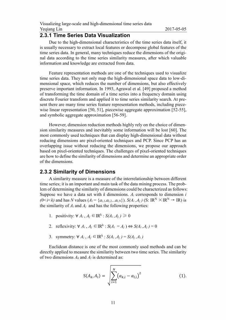
2.3.1 Time Series Data Visualization Due to the high-dimensional characteristics of the time series data itself, it

is usually necessary to extract local features or decompose global features of the time series data. In general, many techniques reduce the dimensions of the origi-nal data according to the time series similarity measures, after which valuable information and knowledge are extracted from data.

Feature representation methods are one of the techniques used to visualize time series data. They not only map the high-dimensional space data to low-di-mensional space, which reduces the number of dimensions, but also effectively preserve important information. In 1993, Agrawal et al. [49] proposed a method of transforming the time domain of a time series into a frequency domain using discrete Fourier transform and applied it to time series similarity search. At pre-sent there are many time series feature representation methods, including piece-wise linear representation [50, 51], piecewise aggregate approximation [52-55], and symbolic aggregate approximation [56-59].

However, dimension reduction methods highly rely on the choice of dimen-sion similarity measures and inevitably some information will be lost [60]. The most commonly used techniques that can display high-dimensional data without reducing dimensions are pixel-oriented techniques and PCP. Since PCP has an overlapping issue without reducing the dimensions, we propose our approach based on pixel-oriented techniques. The challenges of pixel-oriented techniques are how to define the similarity of dimensions and determine an appropriate order of the dimensions.

2.3.2 Similarity of Dimensions A similarity measure is a measure of the interrelationship between different

time series; it is an important and main task of the data mining process. The prob-lem of determining the similarity of dimensions could be characterized as follows: Suppose we have a data set with k dimensions. Ai corresponds to dimension i (0<i<k) and has N values (Ai = {ai,1,ai,2,..ai,N}). S(Ai ,Aj ) (S: IRN ×IRN → IR) is the similarity of Ai and Aj and has the following properties:

1. positivity: ∀ Ai , Aj ∈IRk : S(Ai ,Aj ) ≥ 0

2. reflexivity: ∀ Ai , Aj ∈IRk : S(Ai = Aj ) ⇔ S(Ai ,Aj ) = 0

3. symmetry: ∀ Ai , Aj ∈IRk : S(Ai ,Aj ) = S(Aj ,Ai )

Euclidean distance is one of the most commonly used methods and can be directly applied to measure the similarity between two time series. The similarity of two dimensions Ak and Al is determined as:

S( , ) = , − , (1).


12

However, a similarity measure, which is not even translation invariant, is not useful for practical purposes [12]. Therefore, as a next step, we modify simi-larity to being translation invariant by simply subtracting the mean of the dimen-sion. Thus, we get the following modified similarity measure:

( , ) = , − ( ) − ( , − ( )) (2)

where

mean( ) =1

, (3).

If one additionally demands invariance against scaling, we can scale the di-mension independently such that the maximum value of a dimension becomes 1 and the minimum becomes 0 [12]. Thus, the scaling invariant global similarity measure can be computed as:

( , ) = , − , (4)

where

, = , − min ( )

max( ) − min( ) (5).

This is because Euclidean distance is used to measure time series of equal length and sensitive to abnormal data. Dynamic time warping [61, 62], which matches time series morphologies by bending time axes, can make up for these deficiencies appeared in Euclidean distance. Other approaches used to determine the similarity of two dimensions have been proposed in the context of time series databases [63, 64]. Depending on the application, other similarity measures, for example those described in [65], might be preferable.

2.3.3 Similarity Ordering of Dimensions Arranging the order of dimensions is a common problem in many techniques

such as pixel-oriented and PCP. It plays an important role, among other things, the detection of functional dependencies and correlations (Fig 2.10). The dimen-sion arrangement problem is defined mathematically as an optimization problem which ensures that the most similar dimensions are placed next to each other [12].


13

(a). Sequential arrangement (b). Similarity arrangement

Figure 2.10 The circle segments visualization technique [17].

Suppose we have a d-dimensional data, after we compute the similarity be-tween each pair of dimensions, we can create a following symmetric (d x d) sim-ilarity matrix:

S = ( , ) … ( , )

… … . .( , ) … ( , )

where

S , = , ∀ , = (0, … − 1)

and

S( , ) = 0 ∀ , = (0, … − 1)

S(Ai,Aj) describes the similarity between dimension Ai and Aj. Next, we can create a symmetric (d x d) neighborhood matrix which describes the neighborhood re-lation between the dimensions:

N =, ⋯ ,

… … …, ⋯ ,

where

, = , ∀ , = (0, … − 1)

and

, = 0 ∀ , = (0, … − 1)

and


14

, =1, ℎ0, ℎ

So the optimal similarity order of dimensions is such that

, × ( , )

is minimal.

Ankerst et al. [12] have proved that the ordering of dimensions problem is an NP-complete problem. Yang et al. [11] proposes a dimension hierarchy ap-proach, using a hierarchical cluster tree to generate the similarity order of dimen-sions, which can greatly reduce the time complexity. They first construct a hier-archical cluster tree using an iterative cluster. Then they order each cluster in the dimension hierarchy. For a non-leaf node, they use its representative dimension in the ordering of its parent node. Then, the order of the dimensions is decided in a depth-first traversal of the dimension hierarchy (non-leaf nodes are not counted in the order). Once the order of children of each cluster is decided, the order of all the dimensions is decided. Thus the problem of ordering all the original di-mensions has be converted to ordering the children of non-leaf nodes of the di-mension hierarchy.

Because in most cases, the number of children of a cluster in the dimension hierarchy is much smaller than the number of leaf nodes of that hierarchy, the complexity of the ordering will be greatly reduced. The time cost of an N dimen-sions data set is N!. Suppose using a dimension hierarchy constructs a well-bal-anced M-tree, where M is much smaller than N, the cost will be reduced to ap-proximately (N-1)/(M-1)*M!, which is much less than N!. This is because an N leaf nodes M-tree has (N-1)/(M-1) none-leaf nodes, and each node has M children, the optimal order of a node cost M!.

Table 2.1 Loop times of N! and (N-1)/(M-1)*M!

N N! (N-1)/(M-1)*M!

M=2 M=4 10 3628800 18 72

11 39916800 20 72

12 479001600 22 72

13 6227020800 24 96

14 87178291200 26 96

15 1.30767E+12 28 96

16 2.09228E+13 30 120

17 3.55687E+14 32 120

18 6.40237E+15 34 120

19 1.21645E+17 36 144

20 2.4329E+18 38 144


15

3 Proposed Solution This chapter introduces the new visualization technique pixel video. Since

the time series data are of a temporal nature, we dynamically display the data by video instead of presenting all the data values statically, which is a more effective way of highlighting the temporal nature of data.

We start by briefly introducing the three parts of the work, which is followed by a description of the three components in detail (Fig 3.1). The three parts are the following:

1. Different dimensions could have different ranges, and since we focus on the change of data, we should scale the dimensions independently so that the maximum value of a dimension becomes 1 and the minimum be-comes 0. After normalization of the data, we calculate the correlation and distance between each pair of dimensions.

2. Generation of the similarity order of dimensions. Here, we consider both correlation and distance as similarity measures. We begin by proposing a dimensions clustering algorithm based on correlation and distance, next we construct a hierarchical cluster tree to generate the similarity order of dimensions.

3. Using pixel-oriented techniques to display data and visualize the data in the form of a video.

Figure 3.1 Structure of the work.

Data

pre-process

• ln the first step, after having read the data file, we normalize the data values, then calculate the correlation and distance between each pair of dimensions.

Generate order

• In the second step, we use our algorithm to build a hierarchical cluster tree and generate the similarity order of dimensions through a depth-first traveral of this tree.

Visualization

• In the final step we map data values to color pixels and display the data as a video.


16

3.1 Data Preprocessing In the first part, we normalize the data value, then we calculate the correla-

tion and distance between each pair of dimensions.

3.1.1 Min-Max Normalization In most cases, the range of dimensions is different. For example, the range

of some dimensions are 0 to 100 while other dimensions are -1 to 1. Since we display data dynamically, we focus on the change of data. As mentioned in sec-tion 2.3.2, if one additionally demands invariance against scaling, we can scale the dimension independently such that the maximum value of a dimension be-comes 1 and the minimum becomes 0.

When we read the data, the first step is scaling the data value, in other words, normalize the data by using min-max normalization. After min-max normaliza-tion, the new value is between 0 and 1, which is also convenient for calculating the similarity and color mapping. The variable a is an original value, a’ is new value, mina is the minimum value of the dimension, maxa is the maximum value of the dimension. The formula is shown below.

= −

− (6).

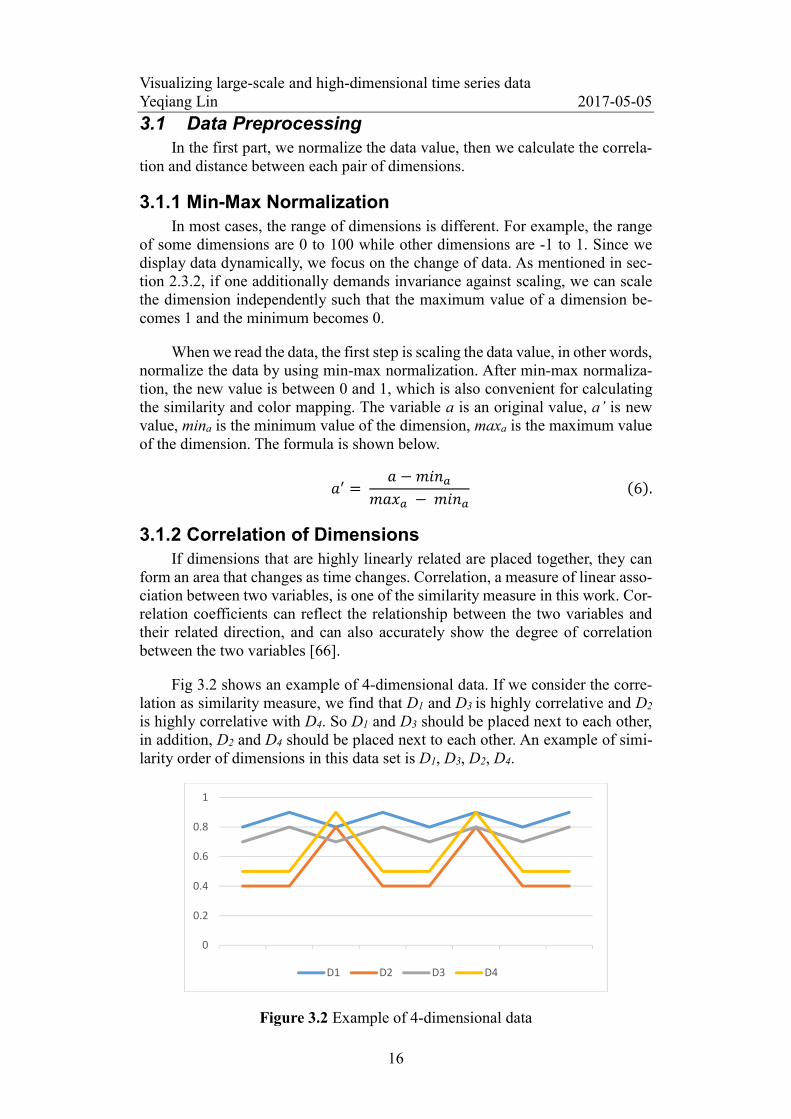
3.1.2 Correlation of Dimensions If dimensions that are highly linearly related are placed together, they can

form an area that changes as time changes. Correlation, a measure of linear asso-ciation between two variables, is one of the similarity measure in this work. Cor-relation coefficients can reflect the relationship between the two variables and their related direction, and can also accurately show the degree of correlation between the two variables [66].

Fig 3.2 shows an example of 4-dimensional data. If we consider the corre-lation as similarity measure, we find that D1 and D3 is highly correlative and D2 is highly correlative with D4. So D1 and D3 should be placed next to each other, in addition, D2 and D4 should be placed next to each other. An example of simi-larity order of dimensions in this data set is D1, D3, D2, D4.

Figure 3.2 Example of 4-dimensional data

0

0.2

0.4

0.6

0.8

1

D1 D2 D3 D4


17

The Pearson correlation coefficient [66] and the Spearman correlation coef-ficient [67] are the most commonly used measures. We use Pearson correlation coefficient as similarity measure in this work, because the Spearman correlation requires a calculation of the rank of each data item, which is a high computational cost in large-scale and high-dimensional data. In addition, Jan and Tomasz [68] have made a comparison of these two measures. Their results show that the sig-nificance of Spearman’s correlation can lead to the significance or non-signifi-cance of Pearson’s correlation coefficient even for big sets of data, which is con-sistent with a logical understanding of the difference between the two coefficients. However, the logical reasoning is not correct in the case of the significance of Pearson’s coefficient translating into the significance of Spearman’s coefficient. A situation is possible where Pearson’s coefficient is positive while Spearman’s coefficient is negative. The results lead to the following conclusion: make sure not to over-interpret Spearman correlation coefficient as a significant meas-ure of the strength of the associations between two variables.

Suppose we have a data set with k dimensions. Ai corresponds to dimension i (0<i<k) and has N values. Let C(Ai,Aj) be the correlation of two dimensions Ai and Aj, the formula is shown below.

C , =∑

∑ ∑

∑∑

∑∑

(7).

3.1.3 Distance of Dimensions In addition to the correlation, another similarity measure to be considered:

the distance among dimensions because the close values can form a bigger color area, increasing the image more readability.

Fig 3.3 shows an example of 4-dimensional data, where we find that D1, D3, D4 are highly correlated. If we only use correlation as similarity measure, one of the similarity orders will be D1, D3, D4, D2.

Figure 3.3 Example of 4-dimensional data.

0

0.2

0.4

0.6

0.8

1

D1 D2 D3 D4


18

However, values in D3 are much smaller than D1, D2 and D4. If we use the pixel-oriented technique and map the data to color pixels, a different color will emerge in the middle of the area (Fig 3.4). To increase image readability, we prefer if the same color can be grouped, making the similarity order D1, D4, D2, D3 (Fig 3.5).

Figure 3.4 Example of pixel-oriented 4-dimensional data

Figure 3.5 Example of pixel-oriented 4-dimensional data

Here, we consider both correlation and distance as similarity measures. Since we have normalized the data, we use Euclidean distance as distance meas-urement.

Suppose we have a data set with k dimensions. Ai corresponds to dimension i (0<i<k) and has N instances. Let D(Ai,Aj) be the distance of two dimensions Ai and Aj, the formula is shown below.

, = ∑ − (8).

3.2 Generating the Similarity Order of Dimensions Yang et al. [11] proposed a general approach to dimension management for

high dimensional visualization, which can also switch the problem of ordering, spacing, and filtering of all the original dimensions to the problem of ordering, spacing, and filtering of the child nodes of each cluster in the dimension hierarchy. This approach can scale down the problems and reduce their complexity. The dimension hierarchy is represented and navigated by a multiple ring structure called InterRing [44].

Here, the dimension hierarchy approach is used to generate the similarity order. We propose a clustering algorithm based on correlation and distance simi-larity, to construct a hierarchal dimension cluster tree to generate the similarity order of dimensions.


19

3.2.1 Similarity Order of Dimensions As discussed in section 2.3.3, once the similarity measures have been de-

fined, the optimal order is the smallest sum of neighboring dimension similarities within the dimensions to be ordered [12]. It is a high computational complexity while finding the optimal order needs to compute all possibilities. The dimension hierarchy approach [11] uses a hierarchical cluster tree to generate the approxi-mate dimension similarity order.

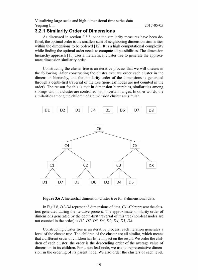
Constructing the cluster tree is an iterative process that we will discuss in the following. After constructing the cluster tree, we order each cluster in the dimension hierarchy, and the similarity order of the dimensions is generated through a depth-first traversal of the tree (non-leaf nodes are not counted in the order). The reason for this is that in dimension hierarchies, similarities among siblings within a cluster are controlled within certain ranges. In other words, the similarities among the children of a dimension cluster are similar.

Figure 3.6 A hierarchal dimension cluster tree for 8-dimensional data.

In Fig 3.6, D1-D8 represent 8 dimensions of data, C1~C6 represent the clus-ters generated during the iterative process. The approximate similarity order of dimensions generated by the depth-first traversal of this tree (non-leaf nodes are not counted in the order) is D1, D7, D3, D6, D2, D4, D5, D8.

Constructing cluster tree is an iterative process; each iteration generates a level of the cluster tree. The children of the cluster are all similar, which means that a different order of children has little impact on the result. We order the chil-dren of each cluster; the order is the descending order of the average value of dimension in its children. For a non-leaf node, we use its representative dimen-sion in the ordering of its parent node. We also order the clusters of each level,


20

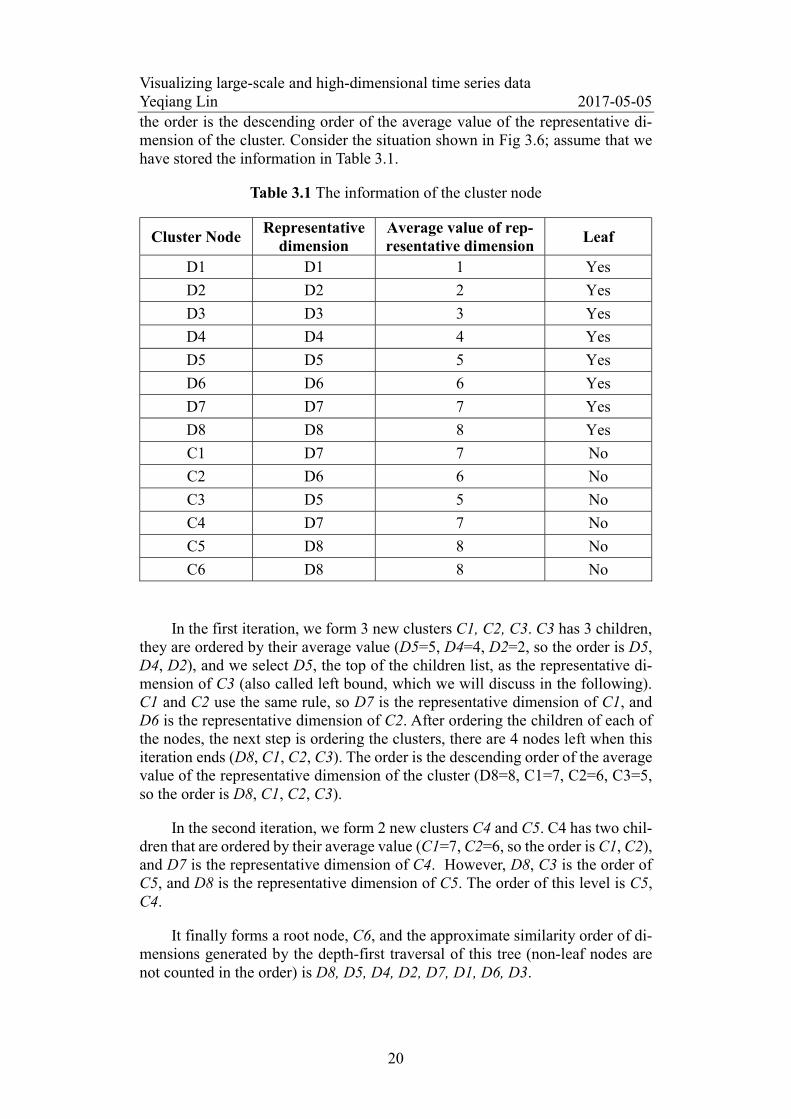
the order is the descending order of the average value of the representative di-mension of the cluster. Consider the situation shown in Fig 3.6; assume that we have stored the information in Table 3.1.

Table 3.1 The information of the cluster node

Cluster Node Representative

dimension Average value of rep-resentative dimension

Leaf

D1 D1 1 Yes

D2 D2 2 Yes

D3 D3 3 Yes

D4 D4 4 Yes

D5 D5 5 Yes

D6 D6 6 Yes

D7 D7 7 Yes

D8 D8 8 Yes

C1 D7 7 No

C2 D6 6 No

C3 D5 5 No

C4 D7 7 No

C5 D8 8 No

C6 D8 8 No

In the first iteration, we form 3 new clusters C1, C2, C3. C3 has 3 children, they are ordered by their average value (D5=5, D4=4, D2=2, so the order is D5, D4, D2), and we select D5, the top of the children list, as the representative di-mension of C3 (also called left bound, which we will discuss in the following). C1 and C2 use the same rule, so D7 is the representative dimension of C1, and D6 is the representative dimension of C2. After ordering the children of each of the nodes, the next step is ordering the clusters, there are 4 nodes left when this iteration ends (D8, C1, C2, C3). The order is the descending order of the average value of the representative dimension of the cluster (D8=8, C1=7, C2=6, C3=5, so the order is D8, C1, C2, C3).

In the second iteration, we form 2 new clusters C4 and C5. C4 has two chil-dren that are ordered by their average value (C1=7, C2=6, so the order is C1, C2), and D7 is the representative dimension of C4. However, D8, C3 is the order of C5, and D8 is the representative dimension of C5. The order of this level is C5, C4.

It finally forms a root node, C6, and the approximate similarity order of di-mensions generated by the depth-first traversal of this tree (non-leaf nodes are not counted in the order) is D8, D5, D4, D2, D7, D1, D6, D3.


21

After ordering the tree, the new cluster tree is as shown in Fig 3.7.

Figure 3.7 A hierarchal dimension cluster tree of 8-dimensional data.

3.2.2 Iterative Process Constructing a hierarchical dimension cluster tree is an iterative process. We

use a bottom-up clustering approach with I times iterations. The iterations consist of the following order: iteration0, iteration1, ..., iterationI. Each iteration has a thresholds Si (0 <= i < I, Si < Sj if i < j, S0 = 1, SI = -1), which is the minimum correlation measures required among the dimensions in a cluster formed. Since the correlation coefficient has range [-1, 1], it guarantees that all dimensions can be included into a root cluster through an iterative clustering process. In addition, when all the dimensions have been grouped to one cluster, the iteration ends.

In the beginning of the iteration, each original dimension corresponds to a leaf node in this tree. There is only one root when the iteration ends. Algorithm 1 shows the iterative process.

Algorithm 1: Iterative Process Input: Current Cluster tree nodes list L, iterative times i Output: New Cluster tree nodes list L.

while L.length > 1 and i < I Clustering in each iteration i++ end


22

When the algotirhm starts, all the original dimensions will be seen as a node and stored in a list L, this means that in the beginning of the iteration the lengh of L is the number of dimensions. I is a user-defined number, it decides the thresholds Si of each iteration. As mentioned above, Si < Sj if i < j, S0 = 1, SI = -1, and the difference between Si and Si+1 is :

1 − (−1)

− 1

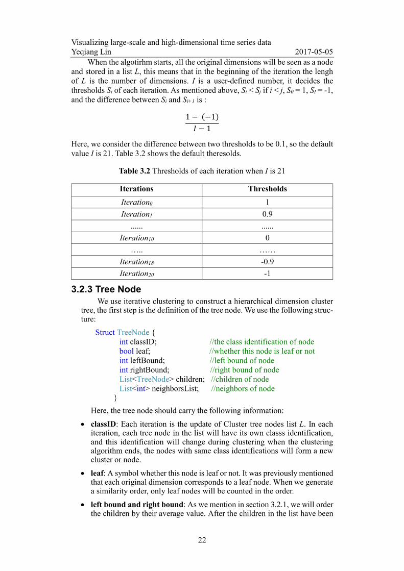
Here, we consider the difference between two thresholds to be 0.1, so the default value I is 21. Table 3.2 shows the default theresolds.

Table 3.2 Thresholds of each iteration when I is 21

Iterations Thresholds

Iteration0 1

Iteration1 0.9

...... ......

Iteration10 0

….. ……

Iteration18 -0.9

Iteration20 -1

3.2.3 Tree Node We use iterative clustering to construct a hierarchical dimension cluster

tree, the first step is the definition of the tree node. We use the following struc-ture:

Struct TreeNode { int classID; //the class identification of node bool leaf; //whether this node is leaf or not

int leftBound; //left bound of node int rightBound; //right bound of node List<TreeNode> children; //children of node List<int> neighborsList; //neighbors of node

}

Here, the tree node should carry the following information:

classID: Each iteration is the update of Cluster tree nodes list L. In each iteration, each tree node in the list will have its own classs identification, and this identification will change during clustering when the clustering algorithm ends, the nodes with same class identifications will form a new cluster or node.

leaf: A symbol whether this node is leaf or not. It was previously mentioned that each original dimension corresponds to a leaf node. When we generate a similarity order, only leaf nodes will be counted in the order.

left bound and right bound: As we mention in section 3.2.1, we will order the children by their average value. After the children in the list have been


23

ordered, the left bound is the head of the list, also called the representative dimension, and the right bound is the tail of the list. When the left bound and the right bound of a node has been defined, the similarity comparison objects between two clusters converts to compare the left bound of a node and the right bound of another node (Fig 3.8). In addition, the left bound and right bound are the same dimension in a leaf node.

Figure 3.8 Two example cluster nodes.

Fig 3.8 shows two example cluster nodes; the similarity between these nodes is actually the similarity between D2 and D7 or the similarity be-tween D1 and D5.

children: A list that stores all the children of this node is used to generate the similarity order of dimensions.

neighborsList: A list that stores all the neighbors of this node is used during clustering.

3.2.4 Proposed Clustering Algorithm As long as the similarity measure between two dimensions is defined, any

one of several existing data clustering algorithms can be used to generate the dimension hierarchy. We proposed a clustering algotithm based on the correlation and distance similarity.

The basic idea of our clustering algorithm is “the most correlated and close dimensions should be grouped first”.

In iterationi, we first construct a nearest neighbor graph, which is different from the K-nearest neighbor graph because the number of neighbors in our graph is uncertain. For each dimension Ai, we create two sets called Ci and Di. In Ci, each element has a Pearson correlation coefficient larger than Si. Then we count the size of Ci, recorded as n, and find its n closest neighbors according to the Euclidean distance, which will form Di. The nearest neibors of Ai is the intersection of Ci and Di. After constructing the nearest neighbor graph, the dimension with its neighbors will form a new cluster.

To avoid some dimensions appearing in more than one cluster, we use the following strategy: Each dimension belongs to the cluster that most of its nearest neighbors belong to. If a dimension have no neighbor or most of the neighbors haven’t formed a new cluster, it and its neighbors that haven’t been clustered form a new cluster.


24

The implementation of each iteration clustering algorithm is shown in Algorithm 2.

Algorithm 2: Clustering Algorithm Input: Current Cluster tree nodes list L, iterative threshold Si. Output: New Cluster tree nodes list L. 1. Search correlative neighbors:

for each node j in node list L do Search other nodes which have Pearson correlation

coefficient with j large than Si, store in C(j). end

2. Search close neighbors and generate nearest neighbors: for each node j in node list L do

Count the number of C(j), recorded as n, search n close neighbors according to Euclidean distance, store in D(j).

j’s nearest neighbors knn(j) = C(j) ∩ D(j). End

3. Clustering: create new node list Lnew for each node j in node list L do

if knn(j) is empty or j.father∈Lnew continue end find the common father node of major of knn(j) = P. if P is NULL

create a new node Pnew, Pnew.addChild(j), L.remove(j). for each node k in knn(j) do

if k.father is NULL Pnew.addChild(k), L.remove(k). end end Pnew .sort() Lnew.add(Pnew).

else if P∈Lnew for each node k in knn(j) do

if k.father is NULL P.addChild(k), L.remove(k). end

end end

end

4. Update the node list L: for each node j in node list Lnew do L.add(j) end L.sort()

5. Calculate the Pearson correlation coefficient and Euclidean

distance between dimensions according to (7) and (8) in Chapter 3.1


25

3.3 Data Visualization After we generate the similarity order of dimensions, the next step is the

color mapping of data values and determining the arrangement of pixels.

3.3.1 Color Mapping Traditional pixel-oriented techniques involve the use of computer algo-

rithms to map out the time series data values using coded color pixels that are able to display much of the information. Color mapping needs to be carefully engineered to be intuitive, because the color coding patterns improvement in the pixel-oriented approach is detrimental to the traditional analysis of time series data, which offers more specificity on data values [69].

Common color mapping models include HSV, RGB, HIS, CHL, and so on. They play a crucial role in their own field. HVS/HSI and RGB models are widely used, we will briefly introduce these three models.

HSV is a color model suitable for the human visual system [70]. In the HSV color model, each color is described by hue, saturation, and value. As a subset of the pyramid in a cylindrical coordinate system, the top of the pyramid of the HSV color model indicates the brightness value is 1, which means that the current color is brightest.

Hue H is determined by the rotation angle with the V axis. Red corresponds to the 0 degree angle, green corresponds to the 120 degree angle, and blue corre-sponds to an angle of 240 degrees. In the HSV model, there is a 180 degree phase difference between each color and its corresponding complementary color. Satu-ration S is in the range 0 to 1, making the top of the pyramid approximately con-ical and has a radius of 1. At the vertex of the pyramid, that is, at its origin, the color is 0, the hue and saturation are not defined, so the point is expressed as black. In the center of the top of the pyramid, the saturation is 0, the color is 1, and the hue is not defined, so the point is expressed as white. The color points between the point of the top surface and the origin of the pyramid are used to represent the decreasing brightness grayscale color. In the gray scale, the satura-tion is 0, and the hue value is not defined (Fig 3.9).

Figure 3.9 HSV color model.


26

Daniel [10] used the HSI model when he decided the pixel-oriented visual-ization techniques. The HSI model is a variation of the HSV model, which de-scribes color by hue, saturation and intensity. In contrast to color scales generated according to the HSV model, linear interpolation within the HIS model provides color scales whose lightness ranges continuously from light to dark. The human eye’s identification ability when it comes to brightness is much greater than the color depth, making the HSI model more in line with the human visual system.

RGB (Red, Green, Blue) is the most used color model. In the three-dimen-sional Cartesian coordinate system, the red, green and blue primary colors are superimposed on each other, resulting in a color system. As shown in Fig 3.10, a cube is used to describe the RGB model, and its main diagonal represents gray scale. In the diagonal, each color has the same brightness, and the coordinates of the origin is black color while the main diagonal vertex is white color. In addition, the remaining six vertexes represent the following different colors: blue, cyan, green, and yellow, red, and magenta.

Figure 3.10 RGB color model.

Here, we use an ordinary RGB model as color mapping (Fig 3. 11) for the following reasons:

1. Data is displayed dynamically, so we are more interested in the change of data rather than the values. There is no need to use the HSI model since the brightness of colors is not a requirement.

2. Linear interpolation between a minimum and a maximum value within the RGB color model is used in our work. Since the data value is between 0 and 1 after scaling, the minimum value is 0 while maximum value is 1.

Figure 3.11 Color Mapping.


27

3.3.2 Arrangement of Pixels The arrangement of pixels is another challenge in pixel-oriented visualiza-

tion techniques. We have introduced some methods arranging the pixels in sec-tion 2.2.1, which are used in many applications. However, traditional sophisti-cated pixel arrangements such as recursive scheme are not suitable in this case, because we data will be displayed in video format; each image does not have to represent a lot of information.

In general, pixel-oriented techniques, such as the recursive pattern technique [15] and the circle segment technique [17], intend to show as much information as possible in one image. They consider both the correlation between each pair of data instances and the correlation between each pair of dimensions, so the im-age can be more meaningful.

Here, we represent data in video format, each frame image displays a little part of the whole data set. So we use the simplest way to arrange the data items from left to right in a line (Fig 3.12).

Figure 3.12 Arrangement of pixels.

3.3.3 Pixel video Each frame represents a time interval of data, the video is played according

the time feature. Many techniques use sliding windows when dealing with time related issues. Here, each frame is a window, the video is a sliding window. The width of the window is a user-defined time unit and the height of the window is the scaling number of dimensions (each dimension or attribute corresponds to one line, the height of one line could larger than 1 pixel). We generate the simi-larity order of dimensions and represent them through different lines, then we arrange the color pixel from left to right. (Fig 3.13).

Because each frame or image now carries much less data, we can use an area of pixels to represent one value. For example, if we use a 1080x1080 image to display 10,000 instances of 100-dimensional data. We can use a 10x10 rectangle to represent one value, so each frame consists of 100 instances, and the length of the video is 100 frames.


28

Figure 3.13 Each frame of pixel video.

3.3.4 Video Playing Mode The hierarchal dimension cluster tree has one root node. The order of all the

dimensions can be generated through the depth-first traversal from the root node. Each iteration creates each level of the tree with a decreasing correlation thresh-old. So we can use multiple windows to display a level of the tree, the depth-firth traversal from each node on the level can generate the order of the corresponding dimensions. Multiple windows can be used to display these nodes, where each sub-window represents each node.

For example, assume that we have a cluster tree as showed in Fig 3.14. If we select the second level, then 2 windows will play the video at the same time (one for C5 and the other one for C4), and the dimensions of each window have the correlation of greater than 0.9. Users can select single window mode or mul-tiple window mode. As a result of displaying multiple windows, dimensions in each sub-window are more correlative and closer, which makes the video more understandable.

Figure 3.14 An example cluster tree.


29

4 Experiment and Discussion This chapter introduces the experiment environment and an evaluation of

the proposed algorithm.

4.1 Experiment Setup We test our work on highly correlated sensor data sets provided in [71]. The

data is publicly available for activity recognition. 230 sensors attached to a hu-man body record values when the user carries out different home activities. Table 4.1 shows the statistics of the data sets (A1~A3 correspond to 3 different activi-ties).

Table 4.1 Statistics of data sets

Data Set Instances Dimension Correlated

A1 51116 230 High A2 33273 230 High A3 32955 230 High

We test our work on a machine with 8GB memory, 4 cores at 2.70GHz. When multiple threads are used, the number of threads is always 8. For visuali-zation purposes, we use the Unity 3D software.

4.2 Evaluation The performance of the hierarchical clustering algorithm is compared to the

traditional hierarchical clustering algorithm AGNES (Agglomerative NESting) [72]. AGNES chooses the most similar two dimensions and forms a new cluster; it stops when all dimensions have been grouped into one cluster (Fig 4.1).

Figure 4.1 AGNES hierarchical clustering.


30

We consider both correlation and distance as a similarity measure in this work. We run AGNES using the following two similarity measures: correlation-based (Pearson correlation coefficient as similarity measure) and distance-based (Euclidean distance as similarity measure).

Optimal order in our work should be to: maximize the sum of correlation and minimize the sum of distance. We use QCD to evaluate the performance of the three algorithms:

Q =

Where SumC is the sum of the dimension correlations, and SumD is the sum of the dimension distances.

Furthermore, we use correlation matrix of data as ground truth. The corre-lation matrix represents the correlation between dimensions, and each matrix cell denotes the correlation of one variable pair. Suppose we have a data set with k dimensions. Ai corresponds to dimension i (0<i<k), Ci,j is the correlation between Ai and Aj. The correlation matrix is shown in the following format:

…, , … , ,

, , … , ,… . . … … … …

, , … , ,

, , … , ,

Since a correlation coefficient has a range of [-1, 1], we use linear interpo-lation between -1 and 1 in the RGB color model to generate a correlation matrix image. Fig 4.2 shows an example of a correlation matrix image.

Figure 4.2 An example correlation matrix image.

In addition, we compare the running time of the three algorithms. Running time is the cost of constructing a cluster tree and generating the order, which is related to the number of dimensions. We test those using different numbers of dimensions.


31

4.3 Result and Discussion In this section, we discuss the performance of the proposed clustering algo-

rithm and visualization.

4.3.1 Clustering algorithm Fig. 4.3 presents the SumC value calculated by three algorithms. The result

shows that correlation-based AGNES always has the greatest SumC value on the three data sets, while the distance-based AGNES always has the smallest SumC on the three data sets.

(a) SumC on data set A1

(b) SumC on data set A2

(c) SumC on data set A3

Figure 4.3 Comparison of SumC (sum of dimension correlations) with distance-based AGNES and correlation-based AGNES.


32

However, Fig. 4.4 presents the SumD value calculated by three algorithms. The result shows that distance-based AGNES always has the greatest SumD value on the three data sets, while correlation-based AGNES always has the smallest SumD on the three data sets.

(a) SumD on data set A1

(b) SumD on data set A2

(c) SumD on data set A2

Figure 4.4 Comparison of SumD (sum of dimension distances) with distance-based AGNES and correlation-based AGNES.


33

It is predictable that both the SumC value and SumD value calculated using our algorithm is between the correlation-based AGNES and distance-based AG-NES. As correlation-based AGNES more focus on correlation between each pair of dimensions, it should have the largest SumC value, just like the distance-based AGNES.

The optimal order has the maximum sum of correlation and minimum sum of distance. Fig. 4.5 presents the QCD value calculated for three algorithms. The results show that our algorithm has the greatest QCD value on all data sets. This means that the proposed algorithm has a better performance when it comes to generating the orders, and also balancing correlation and distance.

(a) QCD on data set A1

(b) QCD on data set A2

(c) QCD on data set A3

Figure 4.5 Comparison of QCD (quotient of SumC and SumD) with distance-based AGNES and correlation-based AGNES.


34

Furthermore, we compare the time cost both in constructing cluster tree and generating order of dimensions, which is related to the number of dimensions. Since all datasets have the same dimensions, the time cost of each algorithm on three data sets is similar. Fig. 4.6 shows that our algorithm is efficient because it requires less time when the number of dimensions increases. The reason for this is that when the number of dimensions increases, AGNES will create more nodes than our algorithm, which means more time is required to construct a cluster tree. Meanwhile, the time cost for depth-first traversing of the tree also increases as the number of tree nodes increase.

We define both correlation and distance as a similarity measure in this work; a balance between these two measures is required. Based on the result we can conclude that the proposed clustering algorithm is more suitable for this work to generate the similarity order of dimensions. This is because our algorithm balances the correlation and distance well, and more inportantly, our algorithm is more efficent when dealing with high-dimensional data.

(a) Running time on data set A1

(b) Running time on data set A2

(c) Running time on data set A3

Figure 4.6 Average running time of 30 runs of three algorithms.


35

4.3.2 Visualization Fig. 4.7 illustrates the correlation matrix of data set A1. The result shows

that there are many dimensions that are highly correlated, and only a few of them are placed next to each other. This is the reason why we need to rearrange the dimensions. In addition, since the time series have a temporal feature, a static display of the data cannot reflect the correlated changes over time, which is the reason why we represent the data in video format.

Figure 4.7 Correlation matrix of data set A1.

Fig. 4.8 shows the visualization result of data set A1. We use two different modes (single and multiple window) and capture frames respectively. The default interval between two frames is one instance, which makes the continuous frames too similar to distinguish. For this reason, we selected one frame every five sec-onds (we use a timer to record the length of the video).

First we discuss the result of single windows (left side of Fig 4.8). The result shows that there are serveral color areas in the image, which correspond to different clusters. Correlated and close dimensions are grouped together so they can generate a correlated change color area. For example, the color in the middle of the frame in the single window changes from red to green, which means the value changes from high to low.

Since single window mode may cause the color staggering, the user can use the multiple window mode, where the sub-windows are more understandable (right side of Fig 4.8). For instance, in multiple window mode, the left top sub-window corresponds to the middle area of a single window, which reflects the change more clearly.

As the related dimensions are grouped together, Pixel video can reflect the temporal correlated changes in the time series. In single window mode and multiple window mode, the user can obverse the changes in data behavior; this could be studied further in future research.


36

(a) Frame image when time = 1s

(b) Frame image when time = 6s

(c) Frame image when time = 11s

(d) Frame image when time = 16s

Figure 4.8 Visualizations of 230 sensors’ time series data. (a) ~ (d) are continuous frame images of single window mode and multiple window mode.


37

5 Conclusions and Future Work 5.1 Summary

Pixel-oriented techniques such as recursive pattern and circle segments are commonly used to visualize large-scale and high-dimensional data. A number of successful visualization techniques have been proposed based on pixel-oriented techniques. Many of which display data statically, trying to show as much infor-mation as possible through one image. However, the human visual system is more sensitive to dynamic changes than static images when it comes to time related issues. Since time series has the temporal nature, dynamically display is a more interesting way to reflect the temporal correlated changes of data.

A visualization technique called the pixel video is presented, displaying large-scale and high-dimensional time series data in video format. It starts by constructing a hierarchal cluster tree to generate the similarity order of dimen-sions, then forms each frame of the video based on the pixel-oriented technique. We consider both correlation and distance as a similarity measure between two dimensions, and propose an efficient clustering algorithm based on the correla-tion and distance similarity to construct a hierarchal cluster tree. Experiments show that the algorithm balances the correlation and distance well, and can gen-erate a similarity order of dimensions effectively. When designing each frame of the video, we map the data to color pixels according to pixel-oriented techniques. When dealing with the challenges of pixel-oriented techniques—color mapping and arrangement of pixels—we compare different approaches and choose the ap-proaches that are suitable for this work. To enhance the readability of the video, we offer users single and multiple window mode, where single window mode provides a global view of data while multiple window mode lets the user drill down the data and makes the video more understandable. Pixel video reflects correlated temporal changes of time series data and offers users a flexible way to explore and study the data.

5.2 Future Work Pixel video is a way for displaying data. In the future, we plan to use the

pixel video techniques as the basis for more visual analytics applications and generate many intuitive and meaningful visualization tools for high-dimensional time series data.

Periodicity analysis is one of the research domains in time series; possible application is periodic pattern recognition. Pixel video offers a timer to record the length of the video, when displays the periodic data, the area formed by cor-related dimensions will show the same changes between two periods. For in-stance, some areas change from green to red every 10 seconds, which means 10 seconds is the period of the area. The system can convert 10 seconds of video to real time units of raw data because it knows how many instances are included in 10 seconds.


38

Another possible application is anomaly detection. The similarity order of dimensions can be generated through training data; once the similarity order of dimensions is decided, the order will not change when displaying new data. By analysing the training data, the system can use techniques such as neural network to predict the color of areas in the next frame image. If the predicted color of these areas is different from the actual color (i.e. predicts red when actual color is green), the system can conclude that the values of these dimensions are abnor-mal.

5.3 Ethical considerations Pixel video can display any type of time series, aiming to reflect the tem-

poral correlated changes of data. The input data is kept private, not any actual content from the data source were published. The result of pixel video does not contain any sensitive or valuable information, the approach itself has no limita-tion.


39

References [1] D. Keim et al. "Information visualization and visual data mining. "

Visualization and Computer Graphics, IEEE Transactions on, 8(1):1–8, 2002.

[2] Liu S., Maljovec D., Wang B., et al. "Visualizing high-dimensional data: Advances in the past decade." IEEE Transactions on Visualization and Computer Graphics, 2017, 23(3): 1249-1268.

[3] Hochheiser, Harry, and Ben Shneiderman. "Dynamic query tools for time series data sets: timebox widgets for interactive exploration." Information Visualization 3, no. 1 (2004): 1-18.

[4] Buono, Paolo, Aleks Aris, Catherine Plaisant, Amir Khella, and Ben Shneiderman. "Interactive pattern search in time series." In Electronic Imaging (2005): 175-186.

[5] Lin, Jessica, Eamonn Keogh, Stefano Lonardi, Jeffrey P. Lankford, and Daonna M. Nystrom. "Viztree: a tool for visually mining and monitoring massive time series databases." In Proceedings of the Thirtieth international conference on VLDB - (2004): 1269-1272.

[6] Abdi H., Williams L J. "Principal component analysis." Wiley interdisciplinary reviews: computational statistics, 2010, 2(4): 433-459.

[7] De Silva V., Tenenbaum J B. "Sparse multidimensional scaling using landmark points." Technical report, Stanford University, 2004.

[8] Inselberg A., Dimsdale B. "Parallel coordinates." Human-Machine Interactive Systems. Springer US, 1991: 199-233.

[9] Inselberg A. "Parallel Coordinates : Visual Multidimensional Geometry and its Applications." Springer, 2009.

[10] Keim D A. "Designing pixel-oriented visualization techniques: Theory and applications." IEEE Transactions on visualization and computer graphics, 2000, 6(1): 59-78.

[11] Yang, Jing, et al. "Interactive hierarchical dimension ordering, spacing and filtering for exploration of high dimensional datasets." Information Visualization, 2003. INFOVIS 2003. IEEE Symposium on. IEEE, 2003.

[12] M. Ankerst, S. Berchtold, and D. A. Keim. "Similarity clustering of di-mensions for an enhanced visualization of multidimensional data. " Proc. of IEEE Symposium on Information Visualization, InfoVis’98, p. 52-60, 1998

[13] Hilbert D. "Ueber die stetige Abbildung einer Line auf ein Flächenstück." Mathematische Annalen, 1891, 38(3): 459-460.


40

[14] Peano G. "Sur une courbe, qui remplit toute une aire plane. " Mathe-matische Annalen, 1890, 36(1): 157-160.

[15] Keim D A., Ankerst M., Kriegel H P. "Recursive pattern: A technique for visualizing very large amounts of data." Proceedings of the 6th Con-ference on Visualization'95. IEEE Computer Society, 1995: 279.

[16] Han J., Pei J., Kamber M. "Data mining: concepts and techniques." Elsevier, 2011.

[17] M. Ankerst, D. A. Keim, and H.-P. Kriegel, “Circle segments: A tech-nique for visually exploring large multidimensional data sets,” in Proc. Visualization 96, Hot Topic Session, San Francisco, CA, 1996.

[18] Asano T., Ranjan D., Roos T., et al. "Space-filling curves and their use in the design of geometric data structures." Theoretical Computer Sci-ence, 1997, 181(1): 3-15.

[19] Wattenberg M. "A note on space-filling visualizations and space-filling curves." Information Visualization, 2005. INFOVIS 2005. IEEE Sympo-sium on. IEEE, 2005: 181-186.

[20] Keim D A., Hao M C., Ladisch J., et al. "Pixel bar charts: A new tech-nique for visualizing large multi-attribute data sets without aggrega-tion." IEEE Symposium on Information Visualization, 2001. INFOVIS 2001. 2001: 113-120.

[21] Yang J., Patro A., Huang S., et al. "Value and relation display for inter-active exploration of high dimensional datasets." Information Visualiza-tion, 2004. INFOVIS 2004. IEEE Symposium on. IEEE, 2004: 73-80.

[22] D. F. Andrews, “Plots of high-dimensional data,” Biometrics, vol. 29, pp. 125–136, 1972.

[23] Cleveland W S. "Visualizing data." Hobart Press, 1993.

[24] Wilkinson L., Anand A., Grossman R L. "Graph-theoretic scagnostics." INFOVIS. 2005, 5: 21.

[25] Wilkinson L., Anand A., Grossman R. "High-dimensional visual analyt-ics: Interactive exploration guided by pairwise views of point distribu-tions." IEEE Transactions on Visualization and Computer Graphics, 2006, 12(6): 1363-1372.

[26] Dang T N., Anand A., Wilkinson L. "Timeseer: Scagnostics for high-di-mensional time series." IEEE Transactions on Visualization and Com-puter Graphics, 2013, 19(3): 470-483.

[27] Tatu A., Albuquerque G., Eisemann M., et al. "Combining automated analysis and visualization techniques for effective exploration of high-


41

dimensional data." Visual Analytics Science and Technology, 2009. VAST 2009. IEEE Symposium on. IEEE, 2009: 59-66.

[28] Ferdosi B J., Roerdink J B T M. "Visualizing High‐Dimensional Struc-tures by Dimension Ordering and Filtering using Subspace Analysis." Computer Graphics Forum. Blackwell Publishing Ltd, 2011, 30(3): 1121-1130.

[29] Ferdosi B J., Buddelmeijer H., Trager S., et al. "Finding and visualizing relevant subspaces for clustering high-dimensional astronomical data using connected morphological operators." Visual Analytics Science and Technology (VAST), 2010 IEEE Symposium on. IEEE, 2010: 35-42.

[30] Peng W., Ward M O., Rundensteiner E A. "Clutter reduction in multi-di-mensional data visualization using dimension reordering." Information Visualization, 2004. INFOVIS 2004. IEEE Symposium on. IEEE, 2004: 89-96.

[31] Yuan X., Guo P., Xiao H., et al. "Scattering points in parallel coord-nates." IEEE Transactions on Visualization and Computer Graphics, 2009, 15(6): 1001-1008.

[32] Claessen J H T., Van Wijk J J. "Flexible linked axes for multivariate data visualization." IEEE Transactions on Visualization and Computer Graphics, 2011, 17(12): 2310-2316.

[33] Fanea E., Carpendale S., Isenberg T. "An interactive 3D integration of parallel coordinates and star glyphs." Information Visualization, 2005. INFOVIS 2005. IEEE Symposium on. IEEE, 2005: 149-156.

[34] Geng Z., Peng Z M., Laramee R S., et al. "Angular histograms: Fre-quency-based visualizations for large, high dimensional data." IEEE Transactions on Visualization and Computer Graphics, 2011, 17(12): 2572-2580.

[35] Chernoff H. "The use of faces to represent points in k-dimensional space graphically." Journal of the American Statistical Association, 1973, 68(342): 361-368.

[36] Correa C D., Chan Y H., Ma K L. "A framework for uncertainty-aware visual analytics." Visual Analytics Science and Technology, 2009. VAST 2009. IEEE Symposium on. IEEE, 2009: 51-58.

[37] Chan Y H., Correa C D., Ma K L. "Flow-based scatterplots for sensitiv-ity analysis." Visual Analytics Science and Technology (VAST), 2010 IEEE Symposium on. IEEE, 2010: 43-50.

[38] Guo Z., Ward M O., Rundensteiner E A., et al. "Pointwise local pattern exploration for sensitivity analysis." Visual Analytics Science and Tech-nology (VAST), 2011 IEEE Conference on. IEEE, 2011: 131-140.


42

[39] Chan Y H., Correa C D., Ma K L. "The generalized sensitivity scatter-plot." IEEE transactions on visualization and computer graphics, 2013, 19(10): 1768-1781.

[40] S. Feiner and C. Beshers, “Visualizing n-dimensional virtual worlds with n-vision,” Computer Graphics, vol. 24, no. 2, pp. 37–38, 1990.

[41] B. Shneiderman, “Tree visualization with treemaps: A 2D space-filling approach,” ACM Transactions on Graphics, vol. 11, no.1, pp. 92–99, 1992.

[42] B. Johnson and B. Shneiderman, “Treemaps: A space-filling approach to the visualization of hierarchical information,” in Proc. Visualization ’91 Conf, 1991, pp. 284–291.

[43] G. G. Robertson, J. D. Mackinlay, and S. K. Card, “Cone trees: Ani-mated 3D visualizations of hierarchical information,” in Proc. Human Factors in Computing Systems CHI 91 Conf., New Orleans, LA, 1991, pp. 189–194.

[44] Yang J., Ward M O., Rundensteiner E A. "Interring: An interactive tool for visually navigating and manipulating hierarchical structures." Infor-mation Visualization, 2002. INFOVIS 2002. IEEE Symposium on. IEEE, 2002: 77-84.

[45] Fua Y H., Ward M O., Rundensteiner E A. "Structure-based brushes: A mechanism for navigating hierarchically organized data and information spaces." IEEE Transactions on visualization and computer graphics, 2000, 6(2): 150-159.

[46] Engel D., Rosenbaum R., Hamann B., et al. "Structural decomposition trees." Computer Graphics Forum. Blackwell Publishing Ltd, 2011, 30(3): 921-930.

[47] Kreuseler M., Schumann H. "A flexible approach for visual data min-ing." IEEE Transactions on Visualization and Computer Graphics, 2002, 8(1): 39-51.

[48] Li H L., Guo C H. "Survey of feature representations and similarity measurements in ime series data mining." Jisuanji Yingyong Yanjiu, 2013, 30(5): 1285-1291.

[49] Agrawal R., Faloutsos C., "Swami A. Efficient similarity search in se-quence databases." Foundations of data organization and algorithms, 1993: 69-84.

[50] Liang J., Zhang J., Yang F., et al. "Study of distance-measuring method and application for time series similarity search based on slope depar-ture." Application Research of Computers, 2010, 1: 017.


43

[51] Hui X., Yunfa H. "Data mining based on segmented time warping dis-tance in time series database." Journal of computer research and devel-opment, 2005, 1: 010.

[52] Keogh E., Chakrabarti K., Pazzani M., et al. "Dimensionality reduction for fast similarity search in large time series databases." Knowledge and information Systems, 2001, 3(3): 263-286.

[53] Hung N., Anh D. "An improvement of PAA for dimensionality reduction in large time series databases." PRICAI 2008: Trends in Artificial Intel-ligence, 2008: 698-707.

[54] Hugueney B., Bouchon-Meunier B. "Time series segmentation and sym-bolic representation, from process-monitoring to data-mining." Interna-tional Conference on Computational Intelligence. Springer Berlin Hei-delberg, 2001: 118-123.

[55] Keogh E., Chakrabarti K., Pazzani M., et al. "Locally adaptive dimen-sionality reduction for indexing large time series databases." ACM SIG-MOD Record, 2001, 30(2): 151-162.

[56] Lin J., Keogh E., Lonardi S., et al. "A symbolic representation of time series, with implications for streaming algorithms." Proceedings of the 8th ACM SIGMOD workshop on Research issues in data mining and knowledge discovery. ACM, 2003: 2-11.

[57] Lin J., Keogh E., Li W., et al. "Experiencing SAX: a novel symbolic representation of time series." Data Mining and knowledge discovery, 2007, 15(2): 107.

[58] Patel P., Keogh E., Lin J., et al. "Mining motifs in massive time series databases." Data Mining, 2002. ICDM 2003. Proceedings. 2002 IEEE International Conference on. IEEE, 2002: 370-377.

[59] Wei L., Kumar N., Lolla V N., et al. "Assumption-Free Anomaly Detec-tion in Time Series." SSDBM. 2005, 5: 237-242.

[60] Lee J A., Verleysen M. "Quality assessment of dimensionality reduction: Rank-based criteria." Neurocomputing, 2009, 72(7): 1431-1443.

[61] Keogh E J., Pazzani M J. "Derivative dynamic time warping." Proceed-ings of the 2001 SIAM International Conference on Data Mining. Soci-ety for Industrial and Applied Mathematics, 2001: 1-11.

[62] Berndt D J., Clifford J. "Using dynamic time warping to find patterns in time series." KDD workshop. 1994, 10(16): 359-370.

[63] Agrawal R., Faloutsos C., Swami A. "Efficient similarity search in se-quence databases." Foundations of data organization and algorithms, 1993: 69-84.


44

[64] Lin R A K., Shim H S S K. "Fast similarity search in the presence of noise, scaling, and translation in time series databases." Proceeding of the 21th International Conference on Very Large Data Bases. 1995: 490-501.

[65] Berchtold S. "Geometry based search of similar parts." Ph. D. Thesis, University of Munich, 1997.

[66] Pearson K. "Notes on the history of correlation." Biometrika, 1920, 13(1): 25-45.

[67] Spearman C. "The proof and measurement of association between two things." The American journal of psychology, 1904, 15(1): 72-101.

[68] Hauke, Jan, and Tomasz Kossowski. "Comparison of values of Pearson's and Spearman's correlation coefficients on the same sets of data." Quaestiones geographicae 30.2 (2011): 87.

[69] Schroeder W J., Lorensen B., Martin K. "The visualization toolkit: an object-oriented approach to 3D graphics." Kitware, 2004.

[70] Holten D., Wijk J J V., Martens J B. "A perceptually based spectral model for isotropic textures." ACM Transactions on Applied Perception (TAP), 2006, 3(4): 376-398.

[71] Roggen, Daniel, Alberto Calatroni, Mirco Rossi, Thomas Holleczek, Kilian Förster, Gerhard Tröster, Paul Lukowicz et al. "Collecting com-plex activity datasets in highly rich networked sensor environments." In Networked Sensing Systems, INSS, (2010): 233-240.

[72] Han, Jiawei, Jian Pei, and Micheline Kamber. "Data mining: concepts and techniques." Elsevier, (2011).

Visualizing large-scale and high-dimensional time series...

Documents

Transcript of Visualizing large-scale and high-dimensional time series...