Mechatronics 22 (2012) 491–502

Contents lists available at SciVerse ScienceDirect

Mechatronics

journal homepage: www.elsevier .com/ locate/mechatronics

Visual control with adaptive dynamical compensation for 3D target trackingby mobile manipulators

Víctor Andaluz a, Ricardo Carelli a,b, Lucio Salinas a,b, Juan Marcos Toibero a,b,⇑, Flavio Roberti a,b

a Instituto de Automática, Universidad Nacional de San Juan, Argentinab Consejo Nacional de Investigaciones Científicas y Técnicas, Argentina

a r t i c l e i n f o

Article history:Available online 24 October 2011

Keywords:Visual controlMobile manipulatorStability analysis3D target tracking

0957-4158/$ - see front matter � 2011 Elsevier Ltd. Adoi:10.1016/j.mechatronics.2011.09.013

⇑ Corresponding author at: Instituto de AutomáticaJuan, Argentina. Tel.: +54 264 4213303; fax: +54 264

E-mail addresses: vandaluz@inaut.unsj.edu.ar (Vunsj.edu.ar (J.M. Toibero).

a b s t r a c t

In this paper an image-based dynamic visual feedback control for mobile manipulators is presented tosolve the target tracking problem in the 3D-workspace. The design of the whole controller is based ontwo cascaded subsystems: a minimum norm visual kinematic controller which complies with the 3D tar-get tracking objective, and an adaptive controller that compensates the dynamics of the mobile manip-ulator. Both the kinematic controller and the adaptive controller are designed to prevent from commandsaturation. Robot commands are defined in terms of reference velocities. Stability and robustness areproved by using Lyapunov’s method. Finally, experimental results are presented to confirm the effective-ness of the proposed visual feedback controller.

� 2011 Elsevier Ltd. All rights reserved.

1. Introduction

In recent years, robotics research has experienced a significantchange. The research interests are moving from the developmentof robots for structured industrial environments to the developmentof autonomous mobile robots operating in unstructured and naturalenvironments. These autonomous mobile robots are applicable in anumber of challenging tasks such as cleaning of hazardous material,surveillance, rescue and reconnaissance in unstructured environ-ments where humans are kept away from. Since it is foreseen thatthis new class of mobile robots will have extensive applications inactivities where human capabilities are needed, they have attractedthe attention of the researchers [1]. Mobile manipulator robot isnowadays a widespread term that refers to robots composed of a ro-botic arm mounted on a mobile platform. This kind of system, whichis usually characterized by a high degree of redundancy, combinesthe manipulability of a fixed-base manipulator with the mobilityof a wheeled platform. Such systems allow the most usual missionsof robotic systems which required both locomotion and manipula-tion abilities. Such systems offer multiple applications in differentindustrial and productive areas as mining and construction or forpeople assistance [2,3].

Robots and intelligent machines need large amounts of informa-tion to autonomously deal with objects in dynamical environments.Visual information has proven to be a highly effective means for

ll rights reserved.

, Universidad Nacional de San4213672.. Andaluz), mtoibero@inaut.

recognizing unknown surroundings. Vision is a useful robotic sen-sor since it mimics the human sense of vision and allows for noncon-tact measurement of the environment. Visual feedback control ofrobotic systems involves the fusion of robot kinematics, dynamics,and computer vision to control the motion of the robot in an effi-cient manner. Visual feedback control is classified into two groups,position based control and image-based control [4]. In position-based control, the references are given in the three-dimensionalCartesian space. The control objective is to bring a relative pose,which is the pose from a camera to a target or from a hand to a tar-get, to a desired pose by using image information. In image-basedcontrol, the references are given in the image plane.

A new tendency is to integrate visual servoing into mobile ro-bots for grasping or manipulation, resulting in a vision-basedautonomous mobile manipulation system [5–11]. Ref. [5] hasdeveloped an image-based visual servo controller for nonholonom-ic mobile manipulators. In this paper, two well-known methods ofredundancy resolution for fixed-base manipulators are extendedfor kinematics modelling of a specific nonholonomic mobilemanipulator. The proposed approach is illustrated only throughcomputer simulation. In [6], authors present a framework ofhand–eye relation for visual servoing with a more global view. Inthis case two mobile manipulators are used, for the main robotthe camera architecture is eye-to-hand configuration, and eye-in-hand configuration for the second robot. Ref. [7] presents a robustvision-based mobile manipulation system for wheeled mobile ro-bots (WMRs). This paper addresses the retention of visual featuresin the field of view of the camera. A hybrid controller for mobilemanipulation is developed to integrate the IBVS controller andthe Q-learning controller through a rule-based supervisor.

492 V. Andaluz et al. / Mechatronics 22 (2012) 491–502

In order to reduce performance degradation, on-line parameteradaptation becomes quite important in applications where the mo-bile manipulator dynamic parameters may vary, such as loadtransportation. It is also useful when there is uncertainty in theknowledge of the dynamic parameters.

In this paper, it is considered a robotic arm mounted on a non-holonomic mobile platform. The mobile manipulator dynamicmodel [12] has, differently to previous works, reference velocitiesas input signals as it is common in commercial robots. It is thenpresented a visual servo controller with adaptive compensation,designed for 3D target tracking by mobile manipulators witheye-in-hand configuration. This controller sets the mobile manipu-lator’s internal configuration and provides the robot the capabilityto avoid obstacles in its path. The design of the controller is basedon two parts, each one being a controller itself. The first one is aminimum norm visual servo controller which avoids saturationsof the velocity commands. It is based on both the mobile manipu-lator’s kinematic model and the vision system model. The secondone is an adaptive dynamic compensation controller, which re-ceives as inputs the velocity references calculated by the kinematiccontroller. The adaptive dynamic compensation controller is capa-ble of updating the estimated parameters, which are directlyrelated to physical parameters of the mobile manipulator. Addi-tionally, it is proved the stability and robustness properties toparametric uncertainties in the dynamic model by using theLyapunov’s method [13]. To validate the proposed control algo-rithms, experimental results are included and discussed.

The main contributions of this paper are: (a) It presents an im-age-based visual control for 3D target tracking of mobile manipu-lators. The controller receives both the estimation of the object’svelocity to be followed and the error image feature to calculatethe control commands as velocity references for the platform andfor the arm, thus achieving a coordinated movement of the wholesystem. Also, the controller is designed including saturation func-tions to limit the control actions within its physical bounds. (b)Two secondary objectives are included in the kinematics controllerdesign by handling the redundancy of the system: the avoidance ofobstacles by the mobile platform and the maximum manipulabilityduring task execution. (c) The design of an adaptive controller toreduce the dynamic parameter uncertainty effects.

This paper is organized as follows. Section 2 presents the kine-matic and dynamic models which have as inputs the velocities ofthe mobile manipulator. Also included in this Section is the projec-tion model of the vision camera. Next, in Section 3, the problemformulation, the vision-based control strategy for the mobilemanipulation system and the design of the kinematic and adaptivedynamic compensation controllers are presented. In Section 4, it isdeveloped the control system stability and robustness analysis. TheExperimental results are presented and discussed in Section 5. Fi-nally, conclusions are given in Section 6.

2. Mobile manipulator models

The mobile manipulator configuration is defined by a vector qof n independent coordinates, called generalized coordinates of themobile manipulator, where q ¼ q1 q2 . . . qn½ �T ¼ qT

p qTa

� �T.

We notice that n = np + na, where np and na are respectively thedimensions of the generalized spaces associated to the mobile plat-form and to the robotic arm. The configuration q is an element ofthe configuration space of the mobile manipulator, denoted by N.The location of the end-effector of the mobile manipulator is givenby the m -dimensional vector h ¼ h1 h2 . . . hm½ �T . Its m coordi-nates are operational coordinates of the mobile manipulator. Theydefine the position and the orientation of the end-effector in R.

The set of all the locations constitutes the operational space of themobile manipulator, denoted by M.

The location of the end-effector of the mobile manipulator canbe defined in different ways according to the task, i.e., it can be con-sidered only the position of the end-effector or both its positionand orientation.

2.1. Kinematic model of the mobile manipulator

The kinematic model of a mobile manipulator represents the loca-tion of its end-effector h as a function of the robotic arm configu-ration and of the platform location (or its operational coordinatesas functions of the robotic arm generalized coordinates and ofthe mobile platform operational coordinates) [25].

f : Na �Mp !M

ðqp;qaÞ# h ¼ fðqp;qaÞ

where, Na is the configuration space of the robotic arm, Mp is theoperational space of the platform.

The instantaneous kinematic model of a mobile manipulatorgivesthe derivative of its end-effector location as a function of the deriv-atives of both the robotic arm configuration and the location of themobile platform,

_h ¼ @f@qðqp;qaÞv

where, _h ¼ _h1_h2 . . . _hm

h iTis the vector of the end-effector

velocity, v ¼ v1 v2 . . . vdn½ �T ¼ vTp vT

a

� �Tis the control vector

of mobility of the mobile manipulator. Its dimension is dn = dnp + dna,where dnp and dna are respectively the dimensions of the controlvector of mobility associated to the mobile platform and to the ro-botic arm. Now, after replacing JgðqÞ ¼ @f

@q ðqp;qaÞ in the above equa-tion, it is obtained

_hðtÞ ¼ JgðqÞvðtÞ ð1Þ

where, Jg(q) is the Jacobian matrix that defines a linear mappingbetween the vector of the mobile manipulator velocities v(t) andthe vector of the end-effector velocity _hðtÞ. The Jacobian matrix is,in general, a function of the configuration q; those configurationsat which Jg(q) is rank-deficient are termed singular kinematic config-urations. It is fundamental to notice that, in general, the dimensionof operational space m is less than the degree of mobility of themobile manipulator. In this case the problem, including the mobilemanipulator and the task, is called to be redundant.

2.2. Dynamic model of the mobile manipulator

The mathematic model that represents the dynamics of a mo-bile manipulator can be obtained from Lagrange’s dynamic equa-tions, which are based on the difference between the kinetic andpotential energy of each of the joints of the robot (energy balance)[14]. The dynamic equation of the mobile manipulator can be rep-resented according to [15] as follows,

MðqÞ _v þ Cðq;vÞv þ GðqÞ ¼ BðqÞs

where, MðqÞ 2 Rdn�dn is a symmetrical positive definite matrix thatrepresents the system’s inertia, Cðq;vÞv 2 Rdn represents the com-ponents of the centripetal and Coriolis forces, GðqÞ 2 Rdn representsthe gravitational forces, B(q) is the input transformation matrix ands 2 Rdn is the torque input vector. For more details on the model see[15].

Most of the commercially available robots have low level PIDcontrollers in order to follow the reference velocity inputs, thusnot allowing controlling the voltages of the motors directly. There-

Fig. 1. Pinhole camera model.

V. Andaluz et al. / Mechatronics 22 (2012) 491–502 493

fore, it becomes useful to express the dynamic model of the mobilemanipulator in a more appropriate way, taking the rotational andlongitudinal reference velocities as the control signals. To do so,the velocity servo controller dynamics are included in the model.The dynamic model of the mobile manipulator, having as controlsignals the reference velocities of the system, can be representedas follows,

MðqÞ _v þ Cðq;vÞv þ GðqÞ ¼ vref ð2Þ

where MðqÞ ¼ H�1ðMþ DÞ;Cðq;vÞ ¼ H�1ðCþ PÞ;GðqÞ ¼ H�1GðqÞ.Thus, MðqÞ 2 Rdn�dn is a positive definite matrix, Cðq;vÞv 2Rdn ;GðqÞ 2 Rdn and vref 2 Rdn is the vector of velocity control signals,H 2 Rdn�dn ;D 2 Rdn�dn and P 2 Rdn�dn are symmetrical diagonal matri-ces, positive definite, that contain the physical parameters of the mo-bile manipulator, motors, velocity controllers of both the mobileplatform and the manipulator robot.

Property 1. Matrix M is positive definite, additionally it is known that

kMðqÞk < kM

Property 2. Furthermore, the following inequalities are also satisfied

kCðq;vÞk < kckvk

Property 3. Vector GðqÞ is bounded

kGðqÞk < kG

where, kc, kM and kG denote some positive constants.

Property 4. The dynamic model of the mobile manipulator can berepresented by

MðqÞ _v þ Cðq;vÞv þ GðqÞ ¼ Lðq;vÞv

where, L(q,v)v2 Rdn�l and v ¼ ½v1 v2 . . . vl�T is the vector of l un-

known parameters of the mobile manipulator, i.e., mass of the mobilerobot, mass of the robotic arm, physical parameters of the mobilemanipulator, motors, velocity, etc. For more details on the model see[12].

For the sake of simplicity, from now on it will be writtenM ¼MðqÞ; C ¼ Cðq;vÞ and G ¼ GðqÞ.

The full mathematical model of the mobile manipulator systemis represented by: (1) the kinematic model and (2) the dynamicmodel, taking the reference velocities of the system as controlsignals.

2.3. Camera projection model

To control the robot using information provided by a computervision system, it is necessary to understand the geometric aspectsof the imaging process. Each camera contains a lens that forms a2D projection of the scene on the image plane where the sensoris located. This projection causes the loss of direct depth percep-tion so that each point on the image plane corresponds to a rayin 3D space. Therefore, some additional information is needed todetermine the 3D coordinates corresponding to an image planepoint. This information may come from multiple cameras, multipleviews with a single camera, or knowledge of the geometric rela-tionship between several feature points on the target. The cameramodel used in this paper is the perspective projection model orpinhole model. It implies a simplified model for an ideal vision cam-era without distortion and optical aberrations.

The pinhole camera model with a perspective projection isshown in Fig. 1. Let fc be a focal length, wpi 2 R3 andcpi ¼ cxi

cyiczi½ �T 2 R3 be the 3D position vectors of the target

object’s ith feature point relative to Ro and Rc, respectively. Rorepresents the world framework and Rc is the camera (end-effec-tor) framework, as Fig. 2 shows. Using a coordinate transformation,the relation between them is,cpi ¼ cRwðwpi � wpCorgÞ ð3Þ

The perspective projection of the i – th feature point onto the im-age plane gives us the image plane coordinate ni ¼ ui v i½ �T 2 R2 as

nicxi;

cyi;czið Þ ¼ � fc

czi

cxi

cyi

� �ð4Þ

Differentiating (3) and (4), it can be expressed _ni in terms of themobile manipulator velocity as

_ni ¼ JIini;

czið ÞcRw 0

0 cRw

� �JgðqÞv � Joi

ðq; cpiÞw _pi ð5Þ

where Jg(q) is the geometric Jacobian of the mobile manipulator de-fined in (1), JIi

ðni;cziÞ is the image Jacobian defined by

JIini;

czið Þ ¼fc

czi0 ui

czi

uiv ifc

f 2c þu2

ifc

v i

0 fcczi

v iczi

f 2c þv2

ifc

uiv ifc

�ui

24 35Moreover, Joi

q; cpið Þw _pi represents the movement of the ith fea-ture point into the image plane, where w _pi is the velocity of the i –th feature point relative to Ro and Joi

q; cpið Þ is defined as

Joi q; cpið Þ ¼ fcczi

1 0 � cxiczi

0 1 � cyiczi

24 35cRw

In applications where objects are located in a 3D space, three ormore image features are required for the visual servo control to besolvable [16,17]. To extend this model to r image points it is neces-sary to stack the vectors of the image plane coordinate, i.e.,

n ¼ ½ nT1 nT

2 . . . nTr �

T 2 R2r ð6Þ

and cp ¼ ½ cp1cp2 . . . cpr �

T 2 R3r . It is assumed that multiplepoint features on a known object are given. From Eq. (5), for multi-ple point features it can be written

_n ¼ Jðq; n; czÞv � Joðq; cpÞw _p ð7Þ

where

Fig. 2. Framework for a dynamic visual feedback system for redundant mobile manipulator.

494 V. Andaluz et al. / Mechatronics 22 (2012) 491–502

Jðq; n; czÞ ¼ JIðn; czÞcRw 0

0 cRw

� �JgðqÞ

JIðn; czÞ ¼

J1 u1 v1½ �T ; cz1

� �...

Jr ur v r½ �T ; czr

� �266664

377775

Joðq; cpÞ ¼ fccz1

1 0 � cx1cz1

0 1 � cy1cz1

24 35 � � � fcczm

1 0 � cxrczr

0 1 � cyrczr

" #24 35T

cRw

For the sake of simplicity, from now on it will be used the fol-lowing notation J = J(q,n, cz) and Jo = Jo(q, cp).

3. Control problem formulation and controllers design

The mobile manipulator robot task is specified in the imageplane in terms of the image feature values corresponding to therelative robot and object positions. Let us denote with nd 2 R2r

the desired image featurevector which is assumed to be constant.For some tasks, the desired feature vector nd can be obtained di-rectly in the image feature space. Another way to get nd is by usinga ‘‘teach-by-showing’’ strategy [18]. In this approach, an image iscaptured at the desired reference position and the correspondingextracted features represent the desired feature vector nd. The con-

Fig. 3. Dynamic visual control for 3D tar

trol problem is to design a controller which computes the appliedvelocities vref to move the mobile manipulator in such a way thatthe actual image features reach the prescribed desired ones. Theproposed control scheme to solve the visual control problem isshown in Fig. 3. The design of the controller is based on two cas-caded subsystems.

(1) Minimum norm kinematic controller with saturation ofvelocity commands, where the image feature error definedas ~n ¼ nd � n may be calculated at every measurement timeand used to drive the mobile manipulator in a directionwhich decreases the error. Therefore, the control aim is toensure that

get track

limt!1

~nðtÞ ¼ 0 2 R2r

(2) Adaptive dynamic compensation controller, which mainobjective is to compensate the dynamics of the mobilemanipulator thus reducing the velocity tracking error. Thiscontroller receives as inputs the desired velocities vc calcu-lated by the kinematic controller, and generates velocity ref-erences vref for the mobile manipulator robot. The velocitycontrol error is defined as ~v ¼ vc � v. Hence, the controlaim is to ensure that

limt!1

~vðtÞ ¼ 0 2 Rdn

ing of mobile manipulators.

V. Andaluz et al. / Mechatronics 22 (2012) 491–502 495

3.1. Minimal norm kinematic controller

The design of the kinematic controller is based on the kinematicmodel of the mobile manipulator and camera projection model.From (7), v can be expressed in terms of _n and w _p by using theright pseudo-inverse of the matrix J

v ¼ J#ð _nþ Jow _pÞ

where, J# = W�1JT(JW�1JT)�1, being W a positive definite matrix thatweighs the control actions of the system,

v ¼W�1JTðJW�1JTÞ�1ð _nþ Jow _pÞ ð8Þ

The controller is based on a minimal norm solution, whichmeans that, at any time, the mobile manipulator will attain its nav-igation target with the smallest number of possible movements.Also the redundancy of the mobile manipulators is effectively usedfor achieving secondary control objectives, such as: avoiding obsta-cles in the workspace and to control the mobile manipulator’s con-figuration. The following control law is proposed for the visualcontrol of the mobile manipulator system,

vc ¼ J#ðJow _pþ LK tanh L�1

K K~n� �

Þ þ ðI� J#JÞLD tanh L�1D Dv0

� �ð9Þ

In (9), Jow _p represents the velocity of the object to be followed

into the image plane, ~n is the vector of control errors defined as~n ¼ nd � n;K 2 R2r ;D 2 Rd; LK 2 R2r and LD 2 Rd are definite posi-tive diagonal matrices that weigh the error vector ~n and the vectorv0, where v0 2 Rd is an arbitrary vector which contains the veloc-ities associated to the mobile manipulator. The first term of theright hand side in (9) describes the primary task of the end effector,i.e., to achieve the desired image features values in order to trackthe moving object. The second term defines self motion of the mo-bile manipulator in which the matrix (I � J#J) projects vector v0

onto the null space of the manipulator Jacobian N(J). This way,the secondary control objectives do not affect the primary task ofthe end-effector. Therefore, any value given to v0 will only changethe internal structure of the manipulator without changing theend-effector location. Thus, the redundancy of the mobile manipu-lators can be effectively used for the achievement of additionalperformances such as: avoiding obstacles in the workspace, avoid-ing singular configurations, or to optimize various performance cri-teria. In this work two different secondary objectives areconsidered: the obstacles avoidance by the mobile platform andthe singular configuration prevention through the system’s manip-ulability control. These secondary objectives are described below.

Fig. 4. Obstacle avo

3.1.1. ManipulabilityWe can observe that one of the main requirements for an accu-

rate task execution by the robot is a good manipulability, definedas the robot configuration that maximizes its ability to manipulatea target object. Therefore, one of the secondary objectives of thecontrol is to maintain maximum manipulability of the mobilemanipulator during task execution. Manipulability is a conceptintroduced by Yoshikawa [19] to measure the ability of a fixedmanipulator to move in certain directions. Bayle [20] presents asimilar analysis for the manipulability of mobile manipulatorsand extends the concept of manipulability ellipsoid as the set ofall end-effector velocities reachable by robot velocities v satisfyingkvk 6 1 in the Euclidean space. A global representative measure ofmanipulation ability can be obtained by considering the volume ofthis ellipsoid which is proportional to the quantity w called themanipulability measure,

w ¼ffiffiffiffiffiffiffiffiffiffiffiffiffiffiffiffiffiffiffiffiffiffiffiffiffiffiffiffiffiffidetðJðqÞJTðqÞÞ

qð10Þ

Therefore, the mobile manipulator will have maximum manip-ulability if its internal configuration is such that maximizes themanipulability measure w.

3.1.2. Obstacle avoidanceThe main idea is to avoid obstacles which maximum height

does not interfere with the robotic arm. Therefore the arm can fol-low the desired path while the mobile platform avoids the obstacleby resourcing to the null space configuration. Fig. 4 shows theobstacle avoidance strategy. The angular velocity and the longitu-dinal velocity of the mobile platform will be affected by a fictitiousrepulsion force. This force depends on both, the incidence angle onthe obstacle a and the distance d to the obstacle. This way, the fol-lowing control velocities are proposed:

uobs ¼ Z�1ðkuobsðdo � dÞ½p=2� jaj�Þ ð11Þxobs ¼ Z�1ðkxobsðdo � dÞsignðaÞ½p=2� jaj�Þ ð12Þ

where, do is the radius which determines the distance at which theobstacle starts to be avoided, ku obs and kx obs are positive adjust-ment gains, the sign function allows defining to which side theobstacle is to be avoided being sign (0) = 1. Z represents themechanical impedance characterizing the robot-environment inter-action, which is calculated as Z = Is2 + Bs + K with I, B and K beingpositive constants representing, respectively, the effect of virtualinertia, damping and elasticity. The closer the platform is to theobstacle, the bigger the values of xobs and uobs.

idance scheme.

496 V. Andaluz et al. / Mechatronics 22 (2012) 491–502

Taking into account the maximum manipulability (10) and theobstacle avoidance (11) and (12), the vector v0 is now defined as,

v0 ¼ �uobs xobs kv1ðh1d� h1Þ kv2ðh2d� h2Þ . . . kvnaðhnad� hnaÞ½ �T

where kviðhid � hiÞ – being i = 1, 2, . . ., na and kvi > 0 – are joint veloc-ities proportional to the configuration errors of the mobile roboticarm, in such a way that the manipulator joints will be pulled tothe desired hid values that maximize manipulability. Note that �uobs

represents a reduction value for the linear velocity in order to ob-tain a cautious behaviour. For this reason, uobs must be subtractedfrom the linear velocity component obtained in the first term of (9).

In order to include an analytical saturation of velocities in themobile manipulator system, it is proposed the use of the tanh (.)function, which limits the error in ~n and the magnitude of vector

v0. The expressions tanh L�1K K~h

� �and tanh L�1

D Dv0

� �denote a

component by component operation.

3.1.3. Stability analysis of the kinematic controllerThe behaviour of the control error ~n is now analyzed assuming -

by now- perfect velocity tracking v � vc;vc ¼ ½uc xc_h1c

_h2c . . . _hnac�T . Note that the desired image feature vector is constant,then it can be concluded that _~n ¼ � _n. Now, by substituting (9) in(7) the following closed loop equation is obtained

_~nþ LK tanh L�1K K~n

� �¼ 0 ð13Þ

For the stability analysis the following Lyapunov candidatefunction is considered

Vð~nÞ ¼ 12

~nT~n ð14Þ

Its time derivative on the trajectories of the system is,

_Vð~nÞ ¼ �~nTLK tanh L�1K K~n

� �< 0 ð15Þ

which implies that ~nðtÞ ! 0 asymptotically.

3.2. Adaptive dynamic compensation

The proposed kinematic controller presented in Section 3.A as-sumes perfect velocity tracking; nevertheless this is not true in realcontexts, mainly when high-speed movements or heavy loadtransportation are required. Therefore, it becomes essential to con-sider the mobile manipulator dynamics, in addition to its kinemat-ics. Furthermore, it is very important to consider that the dynamicparameters of the mobile manipulator may be uncertain due tochanges in dynamics for different tasks. Hence, the velocity errordue to the dynamic effects of the robot and the uncertainties ofthe real dynamic parameters of the mobile manipulator motivatesto design an adaptive dynamic compensation controller with a robustparameter updating law, as shows Fig. 3.

The adaptive dynamic compensation controller receives as in-puts the desired velocities vc calculated by the kinematic control-ler, and generates velocity references vref for the mobilemanipulator robot (see Fig. 3). Hence, disregarding the assumptionof perfect velocity tracking, the velocity error is defined as,

~v ¼ vc � v

The proposed control law is,

vref ¼cMðqÞrþ bCðq;vÞvc þ bGðqÞ ð16Þ

where, vref ¼ ½uref xref_h1ref

_h2ref . . . _hnaref �T ; cMðqÞ; bCðq;vÞ; bGðqÞare de estimated model matrices; and

r ¼ _vc þ Lv tanhðL�1v Kv ~vÞ ð17Þ

with Kv and Lv symmetrical positive definite matrices.Eq. (16) considering the Property 4 can also be written as

vref ¼ Uðq;v;rÞv ð18Þ

where, Uðq;v;rÞv 2 Rdn�l and v = [v1 v2 . . . vl] is the vector of lunknown parameters of the mobile manipulator.

When such parametric errors are considered, control law (18)can be re-written as,

vref ¼ Uv̂ ¼ UvþU~v ¼ Mrþ Cvc þ GþU~v ð19Þ

where, v and v̂ are the real and estimated parameters of the mobilemanipulator, respectively, whereas ~v ¼ v̂� v is the vector ofparameter errors.

In order to obtain the closed-loop equation for the inversedynamics with uncertain model (2) is equated to (19),

M _v þ Cv þ G ¼Mrþ Cvc þ GþU~v

Mðr� _vÞ ¼ �C~v �U~v ð20Þ

and next, (17) is introduced in (20)

_~v ¼ �M�1U~v�M�1C~v � Lv tanhðL�1v Kv ~vÞ ð21Þ

It is now introduced the following Lyapunov candidate function

Vð~v; ~vÞ ¼ 12

~vTHM~v þ 12

~vTc~v ð22Þ

where c 2 Rlxl is a positive definite diagonal matrix and HM is asymmetric and positive definite matrix. The time derivative of theLyapunov candidate function is,

_Vð~v; ~vÞ ¼ �~vTHMLv tanh L�1v Kv ~v

� �� ~vTHC~v � ~vTHU~vþ ~vTc _~v

þ 12

~vTH _M~v

Now, recalling that MðqÞ ¼ H�1ðMþ DÞand Cðq;vÞ ¼ H�1ðCþ PÞ,

_Vð~v; ~vÞ ¼ �~vTHMLv tanh L�1v Kv ~v

� �� ~vTðCþ PÞ~v � ~vTHU~vþ ~vTc _~v

þ 12

~vT _M~v

Due to the well known skew-symmetric property ofð _M� 2CÞ; _Vð~v; ~vÞ reduces to,

_Vð~v; ~vÞ ¼ �~vTHMLv tanh L�1v Kv ~v

� �� ~vTP~v � ~vTHU~v

þ ~vTc _~v ð23Þ

The proposed parameter-updating law for the adaptive dy-namic compensation controller is based on a leakage term, or r-modification [21–23]. By including such term, the obtained robustupdating law is

_̂v ¼ c�1UTH~v � c�1Cv̂ ð24Þ

where C 2 Rlxl is a diagonal positive gain matrix. Notice that (24)can be rewritten as

_̂v ¼ c�1UTH~v � c�1C~v� c�1Cv ð25Þ

Let us now consider that the dynamic parameters can vary, i.e.,v = v(t) and _~v ¼ _̂v� _v. Substituting (25) in (23),

_Vð~v; ~vÞ ¼ �~vTHMLv tanh L�1v Kv ~v

� �� ~vTP~v � ~vTC~v� ~vTCv� ~vTc _v

ð26Þ

Considering small values of ~v, then Lv tanh L�1v Kv ~v

� �� Kv ~v. The

following constants are defined: tC = kmax(C), tc = kmax(c),

lC ¼ vðCÞ;lMKv P ¼ vðHMKvÞ þ vðPÞ, where vðZÞ ¼ffiffiffiffiffiffiffiffiffiffiffiffiffiffiffiffiffiffiffiffikminðZTZÞ

qis

Fig. 5. Experimental framework for a dynamic visual feedback system for mobile manipulator.

V. Andaluz et al. / Mechatronics 22 (2012) 491–502 497

the minimun singular value to Z, kmaxðZÞ ¼ffiffiffiffiffiffiffiffiffiffiffiffiffiffiffiffiffiffiffiffiffikmaxðZTZÞ

qdenotes

the maximum singular value of Z, and kmin(.) and kmax(.) representthe smallest and the biggest eigenvalues of a matrix, respectively.Then, _V can be rewritten as,

_Vð~v; ~vÞ ¼ �lMKv Pk~vk2 � lCk~vk

2 þ tCk~vkkvk þ tck~vkk _vk ð27Þ

Considering f 2 Rþ is a difference square

1fk~vk � fkvk

2

¼ 1f2 k~vk

2 � 2k~vkkvk þ f2kvk2

can be written as

k~vkkvk 6 12f2 k~vk

2 þ f2

2kvk2 ð28Þ

By applying a similar reasoning with g 2 Rþ, it can be obtained

k~vkk _vk 6 12g2 k~vk

2 þ g2

2k _vk2 ð29Þ

Substituting (29) and (28) in (27)

Fig. 6. Image featur

_Vð~v; ~vÞ 6 �lMKv Pk~vk2 � lCk~vk

2 þ tC1

2f2 k~vk2 þ f2

2kvk2

!

þ tc1

2g2 k~vk2 þ g2

2k _vk2

ð30Þ

Eq. (30) can be written in compact form as

_Vð~v; ~vÞ 6 �a1k~vk2 � a2k~vk2 þ q ð31Þ

where, a1 ¼ lMKv P > 0;a2 ¼ lC �lC

2f2 �lc

2g2 > 0 and q ¼ tCf2

2 kvk2þ

tcg2

2 k _vk2, with f and g conveniently selected. Now, from the Lyapu-

nov candidate function Vð~v; ~vÞ ¼ 12

~vTHM~v þ 12

~vTc~v it can be statedthat

V 6 b1k~vk2 þ b2k~vk

2 ð32Þ

where b1 ¼ 12#M; b2 ¼ 1

2#c; #M ¼ kmaxðHMÞ; #c ¼ kmaxðcÞ. Then,

_V 6 �KV þ q ð33Þ

with K ¼ a1b1; a2

b2

n o. Since q is bounded, (33) implies that ~vðtÞ and ~vðtÞ

are finally bounded. Therefore, the r modification term makes theadaptation law more robust at the expense of increasing the errorbound. As q is a function of the minimum singular value of the gainmatrix C of the r modification term, and its values are arbitrary,then the error bound can be made small. In the limit, if C ? 0, then~vðtÞ ! 0 as t ?1, as previously shown.

es trajectories.

Fig. 7. Time evolution C.

Fig. 8. Velocity commands to the mobile platform.

Fig. 9. Joint velocity commands to the robotic arm.

498 V. Andaluz et al. / Mechatronics 22 (2012) 491–502

Remark 1. Note that the updating law (24) needs the H matrix.This matrix includes parameters of the actuators, which can beeasily known and remain constant. Therefore, this is not a relevantconstraint within the adaptive control design.

4. Stability and robustness analysis

The proposed controller presented above considers that thevelocity of the object to be followed w _p is exactly known.

Nevertheless, this is not always possible in a real context. In prac-tice, this velocity will be estimated by using the visual positionsensing of the object, for instance by an a � b filter [24]. This moti-vates to study the image feature error ~n behaviour by consideringthe estimated velocity errors of the object to be followed and alsorelaxing the assumption of perfect velocity tracking.

It is defined the estimation velocity errors of the object into theimage plane as,

e ¼ Joðw _̂p� w _pÞ

Fig. 10. Movement of the mobile manipulator based on the experimental data The position of the mobile manipulator and the position of the target at the same instant areshown. Five different time instants are depicted.

Fig. 11. Time evolution £.

V. Andaluz et al. / Mechatronics 22 (2012) 491–502 499

where w _p and _̂p are the real and estimated velocities of the object,respectively. Hence (13) can now be written as

_~nþ LK tanh L�1K K ~n

� �¼ J~v þ e ð34Þ

Lyapunov candidate function (14) is considered again, whichtime derivative along the trajectories of the system (34) is

_Vð~nÞ ¼ ~nTðJ~v þ eÞ � ~nTLK tanh L�1K K ~n

� �ð35Þ

A sufficient condition for _Vð~nÞ to be negative definite is

~nTLK tanh L�1K K ~n

� ���� ��� > j~nTðJ~v þ eÞj ð36Þ

For large values of ~n, it can be considered thatLK tanhðL�1

K K ~nÞ � LK. Then, (36) can be expressed as

kLKk > kJ~v þ ek ð37Þ

thus making the errors ~n decrease.Now, for small values of ~n; LK tanh L�1

K K ~n� �

� K~n, thus (36) canbe written as,

k~nk > kJ~v þ ek

kminðKÞ

thus implying that the error ~n is bounded by,

k~nk 6 kJ~v þ ek

kminðKÞð38Þ

Hence, it is concluded that the image feature error is ultimatelybounded by the bound kJ~v þ ek=kminðKÞ on a norm of the control er-ror and the estimated velocity error of the object to be followed.

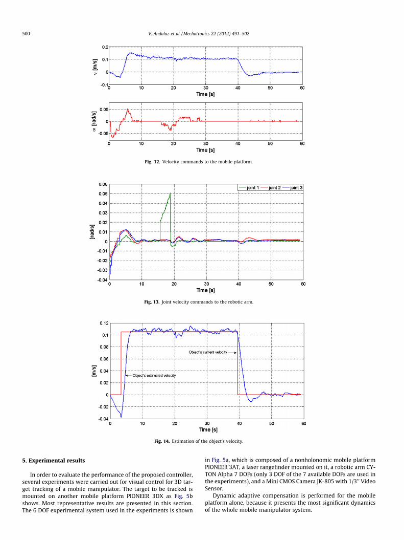
Fig. 12. Velocity commands to the mobile platform.

Fig. 13. Joint velocity commands to the robotic arm.

Fig. 14. Estimation of the object’s velocity.

500 V. Andaluz et al. / Mechatronics 22 (2012) 491–502

5. Experimental results

In order to evaluate the performance of the proposed controller,several experiments were carried out for visual control for 3D tar-get tracking of a mobile manipulator. The target to be tracked ismounted on another mobile platform PIONEER 3DX as Fig. 5bshows. Most representative results are presented in this section.The 6 DOF experimental system used in the experiments is shown

in Fig. 5a, which is composed of a nonholonomic mobile platformPIONEER 3AT, a laser rangefinder mounted on it, a robotic arm CY-TON Alpha 7 DOFs (only 3 DOF of the 7 available DOFs are used inthe experiments), and a Mini CMOS Camera JK-805 with 1/3’’ VideoSensor.

Dynamic adaptive compensation is performed for the mobileplatform alone, because it presents the most significant dynamicsof the whole mobile manipulator system.

Fig. 15. Evolution of the adaptive parameter �.

V. Andaluz et al. / Mechatronics 22 (2012) 491–502 501

For all experiments in this section it was considered an error of25% in model parameters. Also, the positions of the arm joints that

maximize the arm’s manipulability are obtained through numericsimulation. This way, the desired joint angles are: h1d = 0[rad],

502 V. Andaluz et al. / Mechatronics 22 (2012) 491–502

h2d = 0.6065[rad], and h3d = �1.2346[ rad]. Matrix H used in theupdating law is H = diag (33.4,16.7). Also, controller’s gain matricesare set to: K = diag(0.12,0.12,0.12); LK = diag(0.15,0.15,0.15);D = diag(0.14,0.2,0.02,0.02,0.02); LD = diag(0.7,1,0.1,0.1,0.1).

Experiment I: In this experiment, the mobile platform locationis qp = [0 m 0 m 0 rad]T and the robotic arm configuration isqa = [�0.18 0 0]T [rad]; thus, considering that the origin of the im-age coordinates is located at the centre of the image, the initial val-ues of image features initial are n(0) = [u1 v1 v2]T = [�162 �70 68]T

[pixels]. The desired image features vector was defined as nd = [u1

v1 v2]T = [0 �60 65]T [pixels]. Figs. 6–9 show the results of the firstexperiment. Fig. 6 shows the evolution of the image features on theimage plane. Fig. 7 shows that the control errors ~nðtÞ are ultimatelybounded with final values close to zero, i.e. achieving final featureerrors max (jnij) < 5 pixels; while Figs. 8 and 9 show the control ac-tions of the mobile manipulator.

Experiment II: Obstacle avoidance and maximum manipulabil-ity control are considered in this experiment. It is considered thatthe obstacle is placed up to a maximum height that does not inter-fere with the vision camera, so that the end-effector can follow thetarget object even when the platform is avoiding the obstacle.Hence, the task is divided into two different control objectives,i.e., a principal objective: moving target object tracking; and a sec-ondary objective, achieved by taking advantage of the redundancyof the mobile manipulator as explained in Section 3: obstacle avoid-ance and maximum manipulability control. The image features initialvector is n(0) = [u1 v1 v2]T = [156 22 134]T[pixels]. The desired im-age features vector is defined as nd = [u1 v1 v2]T = [0 �50 50]T [pix-els]. It is important to remark that, similar to previous experiment,the origin of the image coordinates is located at the centre of theimage. Figs. 10–15 show the results of the second experiment.From the Fig. 13 and 14 (15 < t < 25[s] approximately) it becomesapparent that the end-effector tracks the moving target objectwhile avoiding the obstacle. Fig. 10 shows the stroboscopic move-ment on the X–Y–Z space. It can be seen the good performance ofthe proposed control system. Fig. 11 shows that the control errors~nðtÞ are ultimately bounded with final values close to zero, i.e.achieving final feature errors max (jnij) < 4 pixels; Figs. 12 and 13show the control actions of the robot, while Fig. 14 representsthe estimation of the object’s velocity. Notice that even with largevelocity estimation errors, like the errors which appear at thebeginning of the experiment, the control errors remain bounded.Finally Fig. 15 shows the evolution of the adaptive parameters,where it can be seen that all the parameters converge to fixedvalues.

6. Conclusions

In this paper an adaptive dynamic visual feedback control formobile manipulators for 3D target tracking has been developed.It was considered the redundancy of the mobile manipulator sys-tem to control the manipulability and for obstacle avoidance. Ithas been also proposed an adaptive controller which updates themobile manipulator dynamics on-line. The design of the wholecontroller was based on two cascaded subsystems: a minimumnorm visual servo kinematic controller which complies with the

3D target tracking objective, and an adaptive dynamic compensa-tion controller that compensates the dynamics of the mobilemanipulator. Both the kinematic controller and the adaptive dy-namic controller have been designed to prevent from commandsaturation. Robot commands were defined in terms of referencevelocities. Stability and robustness are proved by considering theLyapunov’s method. The performance of the proposed controlleris shown through real experiments.

References

[1] Siegwart R, Nourbakhsh I. Introduction to autonomous mobile robots. The MITPress; 2004.

[2] Khatib O. Mobile manipulation: the ronotic assistant. Robots Auton Syst1999;26(2/3):175–83.

[3] Das Y, Russell R, Kircanski N, Goldenberg A. An articulated robotic scanner formine detection – a novel approach to vehicle mounted systems. In:Proceedings of the SPIE conference, Orlando, Florida; 1999. p. 5–9

[4] Hutchinson S, Hager GD, Corke PI. A tutorial on visual servo control. IEEE TransRobot Automat 1996;12(5):651–70.

[5] Luca AD, Oriolo G, Giordano PR. Image-based visual servoing schemes fornonholonomic mobile manipulators. Robotica 2007;25(2):131–45.

[6] Muis A, Ohnishi A. Eye-to-hand approach on eye-in-hand configuration withinreal-time visual servoing. IEEE/ASME Trans Mechatron 2005;10. 404-4010.

[7] Wang Ying, Lang Haoxiang, de Silva Clarence W. A hybrid visual servocontroller for robust grasping by wheeled mobile robots. IEEE/ASME TransMechatron 2009.

[8] Mansard N, Stasse O, Chaumette F, Yokoi K. Visually-guided grasping whilewalking on a humanoid robot. In: Proc. IEEE int. conf. robot. autom., Rome,Italy; April 2007. p. 3041–7.

[9] Yoo WS, Kim J-D, Na SJ. A study on a mobile platform-manipulator weldingsystem for horizontal fillet joints. Mechatronics 2001;11(7):853–68.

[10] Cetin Levent, Uyar Erol. Design and control of a mobile manipulator withstereo vision guidance. Int J Mechatron Manuf Syst 2009;2(3):369–82.

[11] Xu De, Tan Min, Shen Yang. A new simple visual control method based on crossratio invariance. In: International conference on mechatronics & automation;July 2005. p. 370–5.

[12] Andaluz Vı́ctor, Roberti Flavio. Robust control with redundancy resolution anddynamic compensation for mobile manipulators. In: IEEE-ICIT internationalconference on industrial technology; 2010. p. 1449–54.

[13] Slotine J-JE, Li Weiping. Applied nonlinear control. Englewood Cliffs, NewJersey: hentice-Hall; 1991.

[14] Sciavicco L, Siciliano B. Modelling and control of robot manipulators. Springer;2000. p. 84–106.

[15] Hu YM, Guo BH. Modeling and motion planning of a three-link wheeled mobilemanipulator. In: International conference on control, automation and vision;2004. p. 993–8.

[16] Chaumette F, Rives P, Espiau B. Classification and realization of the differentvision-based tasks. In: Hashimoto K, editor. Visual servoing. Singapore: WorldScientific; 1993. p. 199–228.

[17] Hashimoto K, Aoki A, Noritsugu T. Visual servoing with redundant features. In:Proc. 35th conf. decision and control, Kobe, Japan; December 1996. p. 2482–3.

[18] Weiss LE, Sanderson AC, Neuman CP. Dynamic sensor-based control of robotswith visual feedback. IEEE J Robot Automat 1987;3:404–17.

[19] Yoshikawa T. Manipulability of robotic mechanisms. Int J Robot Res1985;4(2):3–9.

[20] Bayle B, Fourquet J-Y. Manipulability analysis for mobile manipulators. In:IEEE international conference on robots & automation; 2001. p. 1251–6.

[21] Kaufman H, Barkana I, Sobel K. Direct adaptive control algorithms, theory andapplications. 2nd ed. New York, USA: Ed: Springer; 1998.

[22] Sastry S, Bodson M. Adaptive control-stability, convergence androbustness. Englewood Cliffs, NJ: Prentice-Hall; 1989.

[23] Nasisi O, Carelli R. Adaptive servo visual robot control. Robot Auton Syst2003;43:51–78.

[24] Kalata P. The tracking index: a generalized parameter for a � b and a – b � ctarget trackers. IEEE Trans Aero Electron Syst 1994;20(2):174–82.

[25] Bayle B, Fourquet J-Y, Renaud M. Manipulability of wheeled mobilemanipulators: application to motion generation. Int J Robot Res2003;22(7):8565–81.