ACTIVE FLOW CONTROL WITH ADAPTIVE ... - Barron …€¦ · The AIFAC toolbox provides advanced...

ACTIVE FLOW CONTROL WITH ADAPTIVE DESIGNTECHNIQUES FOR IMPROVED AIRCRAFT SAFETY

Software Users Manual (SUM)

December 31, 2009

CONTRACT # NND08AA58C

Prepared by:

Jason O. Burkholder Gang Tao, Ph.D. Douglas R. Smith, Ph.D.BARRON ASSOCIATES, INC. UNIVERSITY OF VIRGINIA UNIVERSITY OF WYOMING1410 Sachem Place Elec. & Computer Engineering Mechanical EngineeringSuite 202 351 McCormick Road 1000 E. University AvenueCharlottesville, VA 22901 Charlottesville, VA 22904 Laramie, WY 82071434-973-1215, Ext. 121 434-924-4586 [email protected] [email protected] [email protected]

Distribution:Timothy H. Cox NASAChristopher J. MillerMail Stop 4840D / P.O. Box 273 Mail Stop 1422D / P.O. Box 273NASA Dryden NASA DrydenEdwards, CA 93523 Edwards, CA 93523

DISTRIBUTION STATEMENT B - Distribution authorized to U.S. Government Agencies and their contractors. Otherrequests for this document shall be referred to NASA Langley.

DISTRIBUTION STATEMENT X - Distribution authorized to U.S. Government Agencies and private individuals orenterprises eligible to obtain export-controlled technical data in accordance with NFS 1852.225-70.

STTR Rights: Contract No. NND08AA58C. Barron Associates, Inc., 1410 Sachem Place, Charlottesville, VA 22901-2496.In accordance with DFARS 252.227-7018, expiration of STTR Data Rights is five years after completion of the project,including any follow-on phases. The Governments rights to use, modify, reproduce, release, perform, display, or disclosetechnical data or computer software marked with this legend are restricted during the period shown as provided in paragraph(b)(4) of the Rights in Noncommercial Technical Data and Computer Software-Small Business Innovation Research (SBIR)Program clause contained in the above-identified contract. No restrictions apply after the expiration date shown above.Any reproduction of technical data, computer software, or portions thereof marked with this legend must also reproducethe markings.

CONTENTS CONTENTS

Contents

1 Scope 11.1 Identification . . . . . . . . . . . . . . . . . . . . . . . . . . . . . . . . . . . . . . . . . 11.2 System Overview . . . . . . . . . . . . . . . . . . . . . . . . . . . . . . . . . . . . . . 11.3 Document Overview . . . . . . . . . . . . . . . . . . . . . . . . . . . . . . . . . . . . . 1

2 Referenced Documents 2

3 Software Summary 23.1 Software Application . . . . . . . . . . . . . . . . . . . . . . . . . . . . . . . . . . . . . 23.2 Software Inventory . . . . . . . . . . . . . . . . . . . . . . . . . . . . . . . . . . . . . . 23.3 Software Environment . . . . . . . . . . . . . . . . . . . . . . . . . . . . . . . . . . . . 33.4 Software Organization and Overview of Operation . . . . . . . . . . . . . . . . . . . . . 43.5 Contingencies, Alternate States and Modes of Operation . . . . . . . . . . . . . . . . . 43.6 Security and Privacy . . . . . . . . . . . . . . . . . . . . . . . . . . . . . . . . . . . . . 43.7 Assistance and Problem Reporting . . . . . . . . . . . . . . . . . . . . . . . . . . . . . 4

4 Access To The Software 44.1 First-Time User of the Software . . . . . . . . . . . . . . . . . . . . . . . . . . . . . . . 4

4.1.1 Equipment Familiarization . . . . . . . . . . . . . . . . . . . . . . . . . . . . . 44.1.2 Access Control . . . . . . . . . . . . . . . . . . . . . . . . . . . . . . . . . . . . 44.1.3 Installation and Setup . . . . . . . . . . . . . . . . . . . . . . . . . . . . . . . . 44.1.4 Removal . . . . . . . . . . . . . . . . . . . . . . . . . . . . . . . . . . . . . . . 5

4.2 Initiating a Session . . . . . . . . . . . . . . . . . . . . . . . . . . . . . . . . . . . . . 64.3 Stopping and Suspending Work . . . . . . . . . . . . . . . . . . . . . . . . . . . . . . . 6

5 Processing Reference Guide 65.1 Capabilities . . . . . . . . . . . . . . . . . . . . . . . . . . . . . . . . . . . . . . . . . 65.2 Conventions . . . . . . . . . . . . . . . . . . . . . . . . . . . . . . . . . . . . . . . . . 65.3 Processing Procedures . . . . . . . . . . . . . . . . . . . . . . . . . . . . . . . . . . . . 7

5.3.1 Adaptive Neural Network Inverse . . . . . . . . . . . . . . . . . . . . . . . . . . 75.3.2 Backlash Inverse . . . . . . . . . . . . . . . . . . . . . . . . . . . . . . . . . . . 125.3.3 Backlash Parameter ID . . . . . . . . . . . . . . . . . . . . . . . . . . . . . . . 165.3.4 Cardinal B-Splines Inverse . . . . . . . . . . . . . . . . . . . . . . . . . . . . . . 195.3.5 Dead-zone Inverse . . . . . . . . . . . . . . . . . . . . . . . . . . . . . . . . . . 215.3.6 Dead-zone Parameter ID . . . . . . . . . . . . . . . . . . . . . . . . . . . . . . 245.3.7 Disturbance Rejection . . . . . . . . . . . . . . . . . . . . . . . . . . . . . . . . 285.3.8 Gaussian Radial Basis Functions Inverse . . . . . . . . . . . . . . . . . . . . . . 335.3.9 Taylor Series Inverse . . . . . . . . . . . . . . . . . . . . . . . . . . . . . . . . . 38

5.4 Related Processing . . . . . . . . . . . . . . . . . . . . . . . . . . . . . . . . . . . . . 405.5 Data Backup . . . . . . . . . . . . . . . . . . . . . . . . . . . . . . . . . . . . . . . . . 405.6 Recovery from Errors, Malfunctions, and Emergencies . . . . . . . . . . . . . . . . . . . 405.7 Messages . . . . . . . . . . . . . . . . . . . . . . . . . . . . . . . . . . . . . . . . . . . 405.8 Quick-Reference Guide . . . . . . . . . . . . . . . . . . . . . . . . . . . . . . . . . . . 40

i

CONTENTS CONTENTS

6 Notes 406.1 Abbreviations and Acronyms . . . . . . . . . . . . . . . . . . . . . . . . . . . . . . . . 40

ii

LIST OF FIGURES LIST OF FIGURES

List of Figures

1 AIFAC in Simulink Library Browser . . . . . . . . . . . . . . . . . . . . . . . . . . . . . 62 Actuator Compensation Feedback Control System . . . . . . . . . . . . . . . . . . . . . 73 Adaptive Neural Network Simulink Block . . . . . . . . . . . . . . . . . . . . . . . . . 74 Adaptive Neural Network Simulink Block Parameters . . . . . . . . . . . . . . . . . . . 105 ANN3NI Model . . . . . . . . . . . . . . . . . . . . . . . . . . . . . . . . . . . . . . . 116 ANN3NI State Errors . . . . . . . . . . . . . . . . . . . . . . . . . . . . . . . . . . . . 117 Backlash Inverse Simulink Blocks . . . . . . . . . . . . . . . . . . . . . . . . . . . . . 128 Backlash Characteristic . . . . . . . . . . . . . . . . . . . . . . . . . . . . . . . . . . . 129 Backlash Inverse Simulink Block Parameters . . . . . . . . . . . . . . . . . . . . . . . 1510 Backlash Model Example . . . . . . . . . . . . . . . . . . . . . . . . . . . . . . . . . . 1811 Backlash Input-Output . . . . . . . . . . . . . . . . . . . . . . . . . . . . . . . . . . . 1812 Backlash Parameter Evolution . . . . . . . . . . . . . . . . . . . . . . . . . . . . . . . 1913 Cardinal B-Splines Simulink Block . . . . . . . . . . . . . . . . . . . . . . . . . . . . . 1914 Cardinal B-Splines Simulink Block Parameters . . . . . . . . . . . . . . . . . . . . . . 2015 Cardinal B-Splines Block Simulink Example . . . . . . . . . . . . . . . . . . . . . . . . 2116 Dead-zone Inverse Simulink Blocks . . . . . . . . . . . . . . . . . . . . . . . . . . . . 2117 Dead-zone Characteristic . . . . . . . . . . . . . . . . . . . . . . . . . . . . . . . . . . 2218 Dead-zone Inverse Simulink Block Parameters . . . . . . . . . . . . . . . . . . . . . . 2419 Dead-zone Model Example . . . . . . . . . . . . . . . . . . . . . . . . . . . . . . . . . 2620 Dead-zone Model Input-Output . . . . . . . . . . . . . . . . . . . . . . . . . . . . . . . 2721 Dead-zone Parameter Evolution . . . . . . . . . . . . . . . . . . . . . . . . . . . . . . . 2822 Disturbance Rejection Simulink Block . . . . . . . . . . . . . . . . . . . . . . . . . . . 2823 Disturbance Rejection Control System . . . . . . . . . . . . . . . . . . . . . . . . . . . 2924 Disturbance Rejection Simulink Block Parameters . . . . . . . . . . . . . . . . . . . . 3025 Disturbance Rejection Example Model . . . . . . . . . . . . . . . . . . . . . . . . . . . 3126 Disturbance Rejection Example System Model . . . . . . . . . . . . . . . . . . . . . . . 3227 Disturbance Rejection Example Model Performance . . . . . . . . . . . . . . . . . . . . 3328 Gaussian Radial Basis Function Simulink Block . . . . . . . . . . . . . . . . . . . . . . 3329 Gaussian Radial Basis Functions . . . . . . . . . . . . . . . . . . . . . . . . . . . . . . 3430 Gaussian Radial Basis Functions Simulink Block Parameters . . . . . . . . . . . . . . . 3531 Gaussian RBF Test Harness . . . . . . . . . . . . . . . . . . . . . . . . . . . . . . . . 3632 Gaussian RBF Test Results (Ka = 0.001) . . . . . . . . . . . . . . . . . . . . . . . . . 3733 Gaussian RBF Test Error . . . . . . . . . . . . . . . . . . . . . . . . . . . . . . . . . . 3734 Taylor Series Simulink Block . . . . . . . . . . . . . . . . . . . . . . . . . . . . . . . . 3835 Taylor Series Simulink Block Parameters . . . . . . . . . . . . . . . . . . . . . . . . . 39

iii

Active Flow Control with Adaptive DesignTechniques for Improved Aircraft Safety Software Users Manual

1 Scope

1.1 Identification

This Software Users Manual (SUM) documents AIFAC — the Barron Associates, Inc. Adaptive In-verse For Actuator Compensation toolbox for MATLAB R©, Version 1.0. MATLAB is a product of TheMathWorksTM.

1.2 System Overview

The overall objective of this STTR effort is to evaluate and demonstrate the potential for well-designed,strategically-located synthetic jet actuators to provide improved commercial transport aircraft safety by:(1) delaying wing stall and improving aircraft controllability at high angles of attack and (2) providinglow-cost actuation redundancy to improve controllability in the event of a mechanical control surfacefailure. Delaying flow separation (i.e., wing stall) and providing “back-up” control power could allow anaircraft to recover from adverse conditions (due to a control surface failure, pilot/autopilot error, etc.)that would otherwise result in a loss of control.

Flow control studies have shown that synthetic jet actuators are efficient devices for controllingseparated internal and external flows [1, 2]. Smith et al. [2] and Amitay et al. [1] have used syntheticjet control near the leading edge of an airfoil to prevent boundary layer separation and hence preventstall at high angles of attack. However, an obstacle to the widespread application of synthetic jetactuators for practical flight control is that modulated input signals to achieve closed-loop flow controlobjectives have been shown to be complex. The input signal variables that can be manipulated forcontrol include the number of active jets in the array, and the signal amplitude, waveform, and frequencydelivered to each jet. The control effect from manipulating each of these variables is typically a complexnonlinear function. Developing a comprehensive, wind tunnel-validated model of synthetic jet actuatorsis technically challenging and expensive.

Control techniques, based on the adaptive inverse methodology, overcome prior limitations and setthe stage for practical flight control using synthetic jet actuators to achieve virtual shaping of aerody-namic surfaces. The adaptive controller design is dependent upon the actuation method (e.g., amplitudeor frequency) and the approximation method used to design the adaptive inverse function. The researchteam designed several adaptive controllers and developed the Adaptive Inverse for Actuator Compensa-tion (AIFAC) Toolbox for Simulink R©.1 The AIFAC Toolbox features adaptive inverse controllers basedon previous designs and new approximation-based adaptive controllers, which are widely applicable tosystems, such as active flow control systems, that suffer from complex unknown actuator nonlinearities.

1.3 Document Overview

This SUM shall document installation and usage of the AIFAC computer software configuration item(CSCI).

SBIR DATA RIGHTS: Contract No. NNL08AA06C. Barron Associates, Inc., 1410 Sachem Place,Charlottesville, VA 22901-2496. In accordance with DFARS 252.227-7018, expiration of SBIR DataRights is five years after completion of the project, including any follow-on phases. The Governmentsrights to use, modify, reproduce, release, perform, display, or disclose technical data or computer softwaremarked with this legend are restricted during the period shown as provided in paragraph (b)(4) of theRights in Noncommercial Technical Data and Computer Software-Small Business Innovation Research(SBIR) Program clause contained in the above-identified contract. No restrictions apply after theexpiration date shown above. Any reproduction of technical data, computer software, or portionsthereof marked with this legend must also reproduce the markings.

1www.mathworks.com

Barron Associates, Inc., Proprietary 1


2 Referenced Documents

References

[1] M. Amitay, D. Pitt, V. Kibens, D. E. Parekh, and A. Glezer, “Control of internal flow separationusing synthetic jet actuators,” in Aerospace Sciences Meeting and Exhibit, 38th, no. AIAA-2000-0903, 2000.

[2] D. Smith, M. Amitay, V. Kibens, D. E. Parekh, and A. Glezer, “Modification of the lifting bodyaerodynamics by synthetic jet actuators,” in Aerospace Sciences Meeting and Exhibit, 36th, no.AIAA-98-0209, 1998.

[3] G. Tao, Adaptive Control Design and Analysis. John Wiley & Sons, 2003.

3 Software Summary

3.1 Software Application

The AIFAC toolbox provides advanced adaptive inverse compensation algorithms in the form of Simulinkblock components. These components may be used to develop control applications with the Simulinkmodeling tool. The applications can be tested and refined within the high-fidelity Simulink modelingenvironment. After verification, the Real-Time Workshop code generation tool may be used to generatedeployable C language code for integration in online real-time control systems.

The AIFAC algorithms provide out-of-the-box diagnostic capabilities that are applicable to a widerange of linear and non-linear control problems.

3.2 Software Inventory

The AIFAC software is distributed in either hard or soft format. The hard format distribution is a singleCD with the AIFAC toolbox in the root directory. The soft format distribution is a single compressedarchive with the AIFAC toolbox in the root directory.

The root directory of the distribution contains this user’s manual, the installation script and tool-box implementation. Subdirectories contain the support files, including documentation, examples andWindows runtime.



The root directory contains the following installation files:

AifacSoftwareUsersManual.pdf This user’s guide.aifacFileList.m List of files in the distribution.autorun.inf The distribution CD “autorun” file.BarronAssociatesIncLogo.ico The Barron Associates corporate logo.barron associates, inc.url URL link to the Barron Associates website.htmlHelpHelper.m Integrated HTML help script.installAifacToolbox.m The toolbox installation script.libAifac.mdl The AIFAC library.slblocks.m Simulink library toolbox integration script.

The root directory contains the following implementation files:

ann3layerLogisticSigmoid callback.m backlash callback.mCubicCardinalBSplineApproxsfunc.cpp CubicCardinalBSplineApproxsfunc.mexw32deadzone callback.m disturbanceRejection callback.mdOmega a dv.c dOmega a dv.mexw32gaDetectBacklash.m gaDetectDeadzone.mGaussianRBFsfunc.cpp GaussianRBFsfunc.mexw32grbf callback.m omega c.comega c.mexw32

The “Doc” subdirectory contains the integrated help files:

ann3niHelp.html backlashCharacteristic.pngBacklashHelp.html BarronLogo.pngCubicCardinalBSplineHelp.html deadzoneCharacteristic.pngDeadzoneHelp.html demoAnn3ni.PNGdemoAnn3ni e.PNG demoBacklash.pngdemoCubicCardBSpline.png demoDeadzone.pngdemoDisturbanceRejection.PNG demoDisturbanceRejectionPerformance.pngdemoDisturbanceRejectionSystem.png demoRbf.pngDisturbanceRejectionControlSystem.png DisturbanceRejectionHelp.htmlgaBacklashProgressPlot.png gaDeadzoneProgressPlot.pnggaussianRbfCurve.png GaussianRbfHelp.htmlreferenceSystem.png TaylorSeriesHelp.html

The “Microsoft.VC80.CRT” subdirectory contains Microsoft C/C++ runtime files with which thetoolbox was built. These files are required to run the s-functions:

Microsoft.VC80.CRT.manifest msvcp80.dllmsvcm80.dll msvcr80.dll

3.3 Software Environment

AIFAC is designed for the R2007b release of The MathWorksTM products:



Product VersionMATLAB R© 7.5Simulink R© 7.0Real-Time Workshop R© 7.0xPC TargetTM 3.3

AIFAC is integrated with Simulink so that it is available in the Library Browser tool.

3.4 Software Organization and Overview of Operation

The AIFAC toolbox is a collection of reusable Simlink blocks in Simulink library form. After installation,AIFAC appears as a folder within the Simulink library browser. The blocks may be used like any otherSimulink component. Each block has an integrated help page.

3.5 Contingencies, Alternate States and Modes of Operation

Each AIFAC block is designed to be simulated under the Simulink system, as well as allowing codegeneration for deployment in real-time applications.

3.6 Security and Privacy

The AIFAC toolbox has no security or privacy issues.

3.7 Assistance and Problem Reporting

Direct all problems and inquiries to the report preparer:Barron Associates, Inc1410 Sachem Place, Suite 202Charlottesville, VA 22901(P) 434.973.1215

4 Access To The Software

4.1 First-Time User of the Software

4.1.1 Equipment Familiarization

AIFAC is targeted for a standard Windows XP computer.

4.1.2 Access Control

AIFAC has no access control features beyond the operating system login.

4.1.3 Installation and Setup

The AIFAC toolbox is distributed as both a simple compressed (e.g. zip) file or a CD, both of whichcontain all required resources. The distribution contains a MATLAB script that installs and cleanlyuninstalls the software. This script executes within the MATLAB environment.

The AIFAC distribution includes the script file “installAifacToolbox.m”. This script installs anduninstalls the toolbox. The base installation directory is the Windows “Program Files” path, which isdefined by the environment variable “ProgramFiles”. This path is the default installation location for



all programs, including MATLAB itself. The script will install the toolbox under the folder “BarronAs-sociates”, in the subfolder ”AIFAC”. The AIFAC folder will be added to the end of the MATLAB path,so that the toolbox is accessible by MATLAB and Simulink.

To install the AIFAC toolbox:

1. Extract the toolbox distribution’s compressed contents.

2. Start MATLAB R2007b.

3. Navigate to the directory containing the distribution’s uncompressed contents.

4. At the MATLAB command line, execute the command: installAifacToolbox

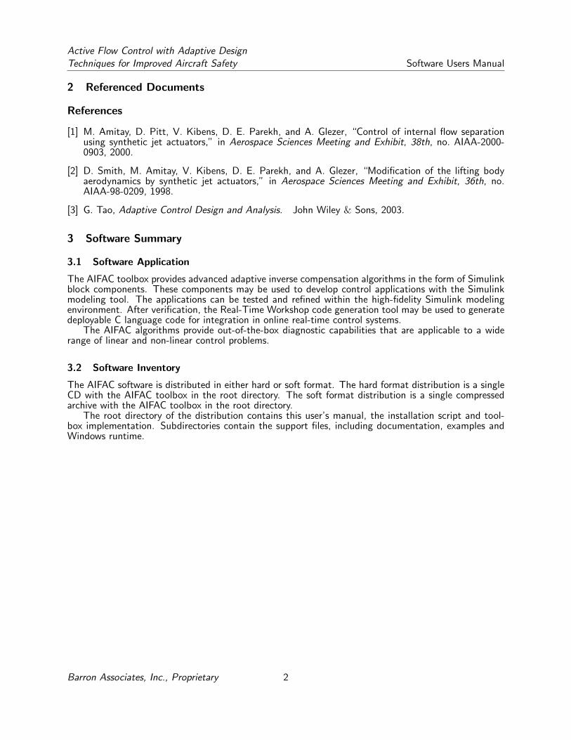
The install script will respond with the following status messages:

>> installAifacToolboxInstalling AIFAC Toolbox

...creating directory C:\Program Files\BarronAssociates

...creating directory C:\Program Files\BarronAssociates\AIFAC

...creating directory C:\Program Files\BarronAssociates\AIFAC\Doc

...creating directory C:\Program Files\BarronAssociates\AIFAC\ToolboxExamples

...creating directory C:\Program Files\BarronAssociates\AIFAC\Microsoft.VC80.CRT

...copying files to C:\Program Files\BarronAssociates\AIFAC

...copying files to C:\Program Files\BarronAssociates\AIFAC\Doc

...copying files to C:\Program Files\BarronAssociates\AIFAC\ToolboxExamples

...copying files to C:\Program Files\BarronAssociates\AIFAC\Microsoft.VC80.CRTAIFAC Toolbox installed; path is ’C:\Program Files\BarronAssociates\AIFAC’

The base path “C:\Program Files” above will be replaced by the system’s “program files” path.After installation, the install program will open this user’s manual.Installation Errors. Either directory creation or file copy could fail if the installer does not have

necessary permissions.The install script could fail to permanently add the toolbox to the MATLAB path if the installer does

not have necessary permissions. In this case, the install script will display the following error message:

** Permanent path modification failed.** Use File->Set Path or the pathtool command to permanently add

the AIFAC toolbox to the MATLAB path.

4.1.4 Removal

The AIFAC installation includes the script file “installAifacToolbox.m”. This script installs and uninstallsthe toolbox.

To uninstall the AIFAC toolbox:

1. Start MATLAB R2007b.

2. At the MATLAB command line, execute the command: installAifacToolbox -uninstall

The install script will respond with the following status messages:

>> installAifacToolbox -uninstallUninstalling AIFAC Toolbox

...deleting directory C:\Program Files\BarronAssociates\AIFAC\Microsoft.VC80.CRT

...deleting directory C:\Program Files\BarronAssociates\AIFAC\ToolboxExamples

...deleting directory C:\Program Files\BarronAssociates\AIFAC\Doc

...deleting directory C:\Program Files\BarronAssociates\AIFACAIFAC Toolbox uninstalled



4.2 Initiating a Session

The AIFAC components appear in the Simulink library browser like any other Simulink block. Openthe library browser by executing “simulink” at the MATLAB command line, or from an open model’stoolbar as shown in Figure 1.

Figure 1: AIFAC in Simulink Library Browser

4.3 Stopping and Suspending Work

This section does not apply.

5 Processing Reference Guide

5.1 Capabilities

The AIFAC Simulink blocks may be used like any other Simulink block, and are compatible with Real-Time Workshop code generation.

5.2 Conventions

All AIFAC blocks are masked, providing a dialog for entering block parameters, including prompts andhelp text.

Each toolbox component has an integrated help page. This page is accessible by selecting the “Help”menu item on the component’s right-click context menu. The help pages contain the following topics:



Overview Provides background information on the block, including its purpose, restrictionsand applicability.

Input Signals Defines each input signal, possibly including dimensionality and restrictions.Output Signals Defines each output signal, possibly including dimensionality and restrictions.Parameters Defines each block parameter, possibly including dimensionality, restrictions and

requirements.Usage Gives guidelines for the block’s usage, including any restrictions.Example Shows an example usage of the component, possibly including simulation results.

5.3 Processing Procedures

The following subsections briefly describe each AIFAC block and its applicability.The generalized feedback control system with adaptive nonlinear inverse is presented in Figure 2:

C1 is the control law, NI is the Nonlinear Inverse, N is the actuator nonlinearity, G is the system withknown dynamics, and C2 is the output feedback.

i G(D)N(·)NI(·)C1(D)

C2(D) �

6

- - - - - -r

−

w ud v u y

Figure 2: Actuator Compensation Feedback Control System

5.3.1 Adaptive Neural Network Inverse

Description

Figure 3: Adaptive Neural NetworkSimulink Block

The Adaptive Neural Network (3-Layer) Non-linear Inverse (ANN3NI ) block provides an adap-tive inverse approximation to an actuator that hasa nonlinear control effect. This block allows thecontroller to treat the actuator’s effect as though itwere linear.

The ANN3NI block is applicable to linear (orlinearizable) systems with measurable system statesand a single nonlinear actuator. The system mayhave any combination of single or multiple in-puts and outputs. The actuator’s nonlinearity(N) must be a scalar function of two variables:N(u d, alpha).

Algorithm The ANN3NI block consists of two neu-ral network (NN) approximators: one approximatorfor the nonlinearity (N) and one for the nonlinearinverse (NI). Each NN has 3-layers. The input layerconsists of two neurons, since the nonlinearity is a



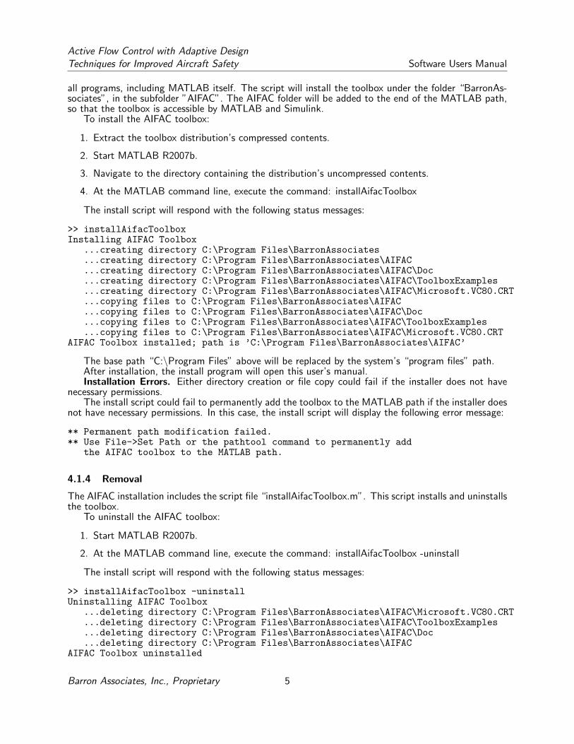
function of two variables. The output layer consists of one neuron, since the NN is approximating ascalar function (N or NI). The number of hidden neurons is defined by the dimensionality of the blockparameters as defined below. More neurons may increase accuracy at the expense of runtime cost. EachNN activation function is the logistical form of the sigmoid:

f(v) =1

(1 + e−av), for a > 0 (1)

Input Signals

u d The desired system input signal, as if the actuator provided linear control.alpha The scalar, second independent actuator nonlinearity input signal.x The measured system state.r The controller input (reference) signal.

Output Signals

v The output signal to drive the actuator to achieve the response desired by u d. The signaldimensions are the same as the input signal u d.

e The error between the desired and actual system response, e = x − xm. The signaldimensions are the same as the system state x.

W The adapted weights for the output layer of the neural network that approximates thenonlinearity (N). These weights may be used in successive simulations to provide moreaccurate initial values in the block’s W parameter. The W dimensions are [n1], where nis the number of hidden neurons defined by the parameters.

W I The adapted weights for the output layer of the neural network that approximates thenonlinear inverse (NI). These weights may be used in successive simulations to providemore accurate initial values in the block’s W I parameter. The W I dimensions are [m1],where m is the number of hidden neurons defined by the parameters.

Parameters and Dialog Box

Advanced settings Advanced settings exposes a configuration option. When this option isnot selected (i.e., not checked), the parameter P is disabled and theblock automatically calculates the P matrix as a solution to the Lya-punov equation PAm+Am′P +Q = 0, where Q is the identity matrixI and Am′ is the transpose of Am. When this option is selected (i.e.,checked), the parameter P is editable and the user may enter his choicefor P . In most cases, the user will want to use the default solution andleave this option unselected. HOWEVER, the default solution requiresthe Control System Toolbox, as the lyap function is needed.

nonlinear actuator index The (one-based) scalar index of the nonlinear actuator’s input signalwithin the system input vector u(t).

A m The system reference model matrix is an estimated system matrix, andis chosen to have all its eigenvalues in Re[s] < 0.

P The P matrix is described above. This field is only editable when the“Advanced Settings” box is checked.

x0 The reference system’s initial states.B The system input matrix.



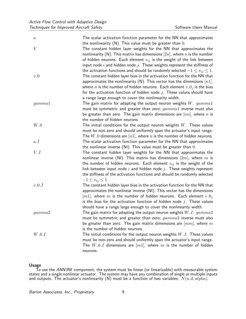
a The scalar activation function parameter for the NN that approximatesthe nonlinearity (N). This value must be greater than 0.

V The constant hidden layer weights for the NN that approximates thenonlinearity (N). This matrix has dimensions [2n], where n is the numberof hidden neurons. Each element vij is the weight of the link betweeninput node i and hidden node j. These weights represent the stiffness ofthe activation functions and should be randomly selected −1 ≤ vij ≤ 1.

v 0 The constant hidden layer bias in the activation function for the NN thatapproximates the nonlinearity (N). This vector has the dimensions [n1],where n is the number of hidden neurons. Each element v 0j is the biasfor the activation function of hidden node j. These values should havea range large enough to cover the nonlinearity width.

gamma1 The gain matrix for adapting the output neuron weights W . gamma1must be symmetric and greater than zero; gamma1 inverse must alsobe greater than zero. The gain matrix dimensions are [nn], where n isthe number of hidden neurons.

W 0 The initial conditions for the output neuron weights W . These valuesmust be non-zero and should uniformly span the actuator’s input range.The W 0 dimensions are [n1], where n is the number of hidden neurons.

a I The scalar activation function parameter for the NN that approximatesthe nonlinear inverse (NI). This value must be greater than 0.

V I The constant hidden layer weights for the NN that approximates thenonlinear inverse (NI). This matrix has dimensions [2m], where m isthe number of hidden neurons. Each element vij is the weight of thelink between input node i and hidden node j. These weights representthe stiffness of the activation functions and should be randomly selected−1 ≤ vij ≤ 1.

v 0 I The constant hidden layer bias in the activation function for the NN thatapproximates the nonlinear inverse (NI). This vector has the dimensions[m1], where m is the number of hidden neurons. Each element v 0jis the bias for the activation function of hidden node j. These valuesshould have a range large enough to cover the nonlinearity width.

gamma2 The gain matrix for adapting the output neuron weights W I. gamma2must be symmetric and greater than zero; gamma2 inverse must alsobe greater than zero. The gain matrix dimensions are [mm], where mis the number of hidden neurons.

W 0 I The initial conditions for the output neuron weights W I. These valuesmust be non-zero and should uniformly span the actuator’s input range.The W 0 I dimensions are [m1], where m is the number of hiddenneurons.

UsageTo use the ANN3NI component, the system must be linear (or linearizable) with measurable system

states and a single nonlinear actuator. The system may have any combination of single or multiple inputsand outputs. The actuator’s nonlinearity (N) must be a function of two variables: N(u d, alpha).



Figure 4: Adaptive Neural Network Simulink Block Parameters

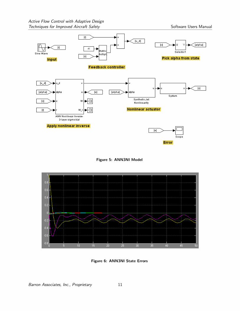
The engineer will decide upon some number of hidden nodes and perform simulations to evaluateperformance. This number may be increased or decreased to achieve a balance between accuracy andspeed. The adaptive output layer weights (W and W I) may be output to the workspace or a file, andserve as initial conditions (W 0 and W 0 I) to subsequent runs in order to start off with more accuracy.

ExampleConsider an aircraft model with the states x = [α p β q r]T where α and β are the angle of

attack and sideslip angles, and p, q, and r are the roll, pitch, and yaw rates, respectively. The controlinputs are u = [δe δa δr]T , which are the elevator, aileron, and rudder deflection angles, respectively.The elevator deflection angle δe is implemented through a synthetic jet actuator.

Since the width of the nonlinearity is −20.076 to 25, the bias vectors v0 and v0 I can be initializedbetween −30 to +30. The output weight initial conditions W0 and W0 I are chosen to be uniformlyrandomly distributed between −50 to +50. The simulation model is shown in Figure 5.

Using system matrices representative of a commercial transport aircraft, we conducted a set ofsimulations. The system is driven by sinusoidal inputs applied to all three control surfaces. The numberof neurons was steadily increased until acceptable performance was attained at n = m = 20 hiddenneurons for both approximators. The state errors are shown in Figure 6.



Figure 5: ANN3NI Model

Figure 6: ANN3NI State Errors



5.3.2 Backlash Inverse

Description

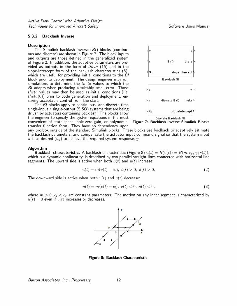
Figure 7: Backlash Inverse Simulink Blocks

The Simulink backlash inverse (BI ) blocks (continu-ous and discrete) are shown in Figure 7. The block inputsand outputs are those defined in the generalized systemof Figure 2. In addition, the adaptive parameters are pro-vided as outputs in the form of theta (16) and in theslope-intercept form of the backlash characteristics (6),which are useful for providing initial conditions to the BIblock prior to deployment. The design engineer may runsimulations to determine the theta values to which theBI adapts when producing a suitably small error. Thosetheta values may then be used as initial conditions (i.e.theta(0)) prior to code generation and deployment, en-suring acceptable control from the start.

The BI blocks apply to continuous- and discrete-timesingle-input / single-output (SISO) systems that are beingdriven by actuators containing backlash. The blocks allowthe engineer to specify the system equations in the mostconvenient of state-space, pole-zero-gain, or polynomialtransfer function form. They have no dependency uponany toolbox outside of the standard Simulink blocks. These blocks use feedback to adaptively estimatethe backlash parameters, and compensate the actuator input command signal so that the system inputu is as desired (ud) to achieve the required system response, y.

AlgorithmBacklash characteristic. A backlash characteristic (Figure 8) u(t) = B(v(t)) = B(m, cr, cl; v(t)),

which is a dynamic nonlinearity, is described by two parallel straight lines connected with horizontal linesegments. The upward side is active when both v(t) and u(t) increase:

u(t) = m(v(t)− cr), v(t) > 0, u(t) > 0. (2)

The downward side is active when both v(t) and u(t) decrease:

u(t) = m(v(t)− cl), v(t) < 0, u(t) < 0, (3)

where m > 0, cl < cr are constant parameters. The motion on any inner segment is characterized byu(t) = 0 even if v(t) increases or decreases.

Figure 8: Backlash Characteristic



A compact description of the backlash characteristic B(·) is

u(t) =

mv(t) if v(t) > 0 and u(t) = m(v(t)− cr) or

if v(t) < 0 and u(t) = m(v(t)− cl),0 otherwise.

(4)

A backlash characteristic in discrete time can be described as

u(t) = B(v(t)) =

m(v(t)− cl) if v(t) ≤ vl,m(v(t)− cr) if v(t) ≥ vr,u(t− 1) if vl < v(t) < vr,

(5)

where the v-axis projections vl and vr of the intersections of the two parallel lines of slope m with thehorizontal inner segment containing u(t− 1) are

vl =u(t− 1)m

+ cl, vr =u(t− 1)m

+ cr. (6)

For a parametrized nonlinearity N(·), we will develop an adaptive inverse as a compensator forcanceling N(·) with unknown parameters.

Backlash inverse. Let the estimates of the backlash parameters m, cr, cl be m, cl, cr. A backlashinverse v(t) = BI(ud(t)) is described by

v(t) =

1mud(t) if ud(t) > 0 and v(t) = ud(t)

m+ cr or

if ud(t) < 0 and v(t) = ud(t)

m+ cl,

0 if ud(t) = 0,

g(t, t) if ud(t) > 0 and v(t) = ud(t)

m+ cl,

−g(t, t) if ud(t) < 0 and v(t) = ud(t)

m+ cr,

(7)

where, with the Dirac δ-function δ(t),

g(τ, t) = δ(τ − t)(cr − cl). (8)

The signal motion of v(t) and ud(t) of the backlash inverse is on two straight lines and verticaljumps between the lines, where the downward side line is

v(t) =ud(t)m

+ cl, ud(t) < 0, (9)

and the upward side line is

v(t) =ud(t)m

+ cr, ud(t) > 0. (10)

Vertical jumps of v(t) occur whenever ud(t) changes its sign: from the downward line to the upwardline if from ud(t) < 0 to ud(t) > 0 or from the upward line to the downward line if from ud(t) > 0 toud(t) < 0.

The discrete-time backlash inverse v(t) = BI(ud(t)) is

v(t) =

v(t− 1) if ud(t) = ud(t− 1),ud(t)

m+ cl if ud(t) < ud(t− 1),

ud(t)

m+ cr if ud(t) > ud(t− 1).

(11)



The backlash inverse has the desired property

ud(t0) = B(BI(ud(t0)))⇒ B(BI(ud(t))) = ud(t), ∀t ≥ t0, (12)

where BI(·) = BI(·)|m=m,cl=cl,cr=cr, the exact backlash inverse.

To parametrize the above backlash inverse, using the indicator function χ, we introduce the backlashinverse indicator functions

χr(t) = χ[v(t) = ud(t)

m+ cr], (13)

χl(t) = χ[v(t) = ud(t)

m+ cl] (14)

and the backlash indicator functions

χr(t) = χ[u(t) > 0], χl(t) = χ[u(t) < 0], χs(t) = χ[u(t) = 0]. (15)

With mcr = mcr, mcl = mcl, we also introduce

θ = [mcr, m, mcl]T , (16)

θ∗ = [mcr,m,mcl]T , (17)

ω(t) = [χr(t),−v(t), χl(t)]T . (18)

It can be verified thatud(t) = −θTω(t), (19)

u(t)− ud(t) = (θ − θ∗)Tω(t) + dN (t), (20)

where, with us being the value of u(t) when u(t) = 0,

dN (t) = (χr(t)− χr(t))(m(v(t)− cr))+ (χl(t)− χl(t))(m(v(t)− cl)) + χs(t)us. (21)

Input Signals

r The input signal to the actuator’s controller (e.g. pilot stick input).ud The desired signal input to an ideal (i.e. no backlash) actuator that would achieve the

response dictated by the reference signal, r.y The measured system response to the actuator control.

Output Signals

v The compensated actuator driving signal that will achieve the desired systemresponse.

theta The adapting nonlinear inverse parameters, in an internal form.slopeIntercept The adapting nonlinear inverse parameters, [m, cr, cl].




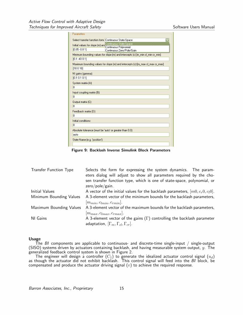
Figure 9: Backlash Inverse Simulink Block Parameters

Transfer Function Type Selects the form for expressing the system dynamics. The param-eters dialog will adjust to show all parameters required by the cho-sen transfer function type, which is one of state-space, polynomial, orzero/pole/gain.

Initial Values A vector of the initial values for the backlash parameters, [m0, cr0, cl0].Minimum Bounding Values A 3-element vector of the minimum bounds for the backlash parameters,

[mmin, clmin, crmin].Maximum Bounding Values A 3-element vector of the maximum bounds for the backlash parameters,

[mmax, clmax, crmax].NI Gains A 3-element vector of the gains (Γ) controlling the backlash parameter

adaptation, [Γm,Γcl,Γcr].

UsageThe BI components are applicable to continuous- and discrete-time single-input / single-output

(SISO) systems driven by actuators containing backlash, and having measurable system output, y. Thegeneralized feedback control system is shown in Figure 2.

The engineer will design a controller (C1) to generate the idealized actuator control signal (ud)as though the actuator did not exhibit backlash. This control signal will feed into the BI block, becompensated and produce the actuator driving signal (v) to achieve the required response.



5.3.3 Backlash Parameter ID

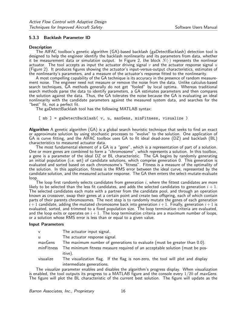
DescriptionThe AIFAC toolbox’s genetic algorithm (GA)-based backlash (gaDetectBacklash) detection tool is

designed to help the engineer identify the backlash nonlinearity and its parameters from data, whetherit be measurement data or simulation output. In Figure 2, the block N(·) represents the nonlinearactuator. The tool accepts as input the actuator driving signal v and the actuator response signal u(Figure 2). It produces figures showing the actuator’s input-versus-output characteristics, estimates ofthe nonlinearity’s parameters, and a measure of the actuator’s response fitted to the nonlinearity.

A most compelling capability of the GA technique is its accuracy in the presence of random measure-ment noise. The engineer need not measure or remove the noise from the data. Unlike calculus-basedsearch techniques, GA methods generally do not get “fooled” by local optima. Whereas traditionalsearch methods parse the data to identify parameters, a GA estimates parameters and then comparesthe solution against the data. Thus, the GA tolerates the noise because the GA is evaluating an idealnonlinearity with the candidate parameters against the measured system data, and searches for the“best” fit, not a perfect fit.

The gaDetectBacklash tool has the following MATLAB syntax:

[ mb ] = gaDetectBacklash( v, u, maxGens, minFitness, visualize )

Algorithm A genetic algorithm (GA) is a global search heuristic technique that seeks to find an exactor approximate solution by using stochastic processes to “evolve” to the solution. One application ofGA is curve fitting, and the AIFAC toolbox uses GA to fit ideal dead-zone (DZ) and backlash (BL)characteristics to measured actuator data.

The most fundamental element of a GA is a “gene”, which is a representation of part of a solution.One or more genes are combined to form a “chromosome”, which represents a solution. In this toolbox,a gene is a parameter of the ideal DZ or BL characteristic. The GA begins by randomly generatingan initial population (i.e. set) of candidate solutions, which comprise generation 0. This generation isevaluated and sorted based on each chromosome’s “fitness”. Fitness is a measure of the optimality ofthe solution. In this application, fitness is the RMS error between the ideal curve, represented by thecandidate solution, and the measured actuator response. The GA then enters the select-mutate-evaluateloop.

The loop first randomly selects candidates from generation i, where the fittest candidates are morelikely to be selected than the less fit candidates, and adds the selected candidates to generation i+ 1.The selected candidates each mate with a partner from the candidate pool, and through an operationknown as crossover, swap their genes at a certain point and create two offspring, each of which containparts of their parents chromosomes. The next step is to randomly mutate the genes of each generationi+ 1 candidate, adding the mutated chromosome back into generation i+ 1. Finally, generation i+ 1 isevaluated, sorted, and trimmed to a fixed population size. The loop termination criteria are evaluated,and the loop exits or operates on i+ 1. The loop termination criteria are a maximum number of loops,or a solution whose RMS error is less than or equal to a given value.

Input Parameters

v The actuator input signal.u The actuator response signal.maxGens The maximum number of generations to evaluate (must be greater than 0.0).minFitness The minimum fitness measure required of an acceptable solution (must be pos-

itive).visualize The visualization flag. If the flag is non-zero, the tool will plot and display

intermediate generations.The visualize parameter enables and disables the algorithm’s progress display. When visualization

is enabled, the tool outputs its progress to a MATLAB figure and the console every 1/20 of maxGens.The figure will plot the BL characteristic of the current best solution. The figure will update as the



generations are finished, providing an animated progress indication. The console will show the currentbest solution and its fitness.

The maxGens parameter limits the number of generations that the GA uses to develop a solution.The more generations, the longer the runtime and the more accurate the BL parameters up to a limitimposed by the noise in the signals. This parameter is the primary means of limiting the tool’s runtime.In general, the engineer should start with a value of 1000. Adjust the parameter upwards if the resultingfitness is not acceptable. Visualization may indicate that RMS error does not decrease below a certainvalue due to the noise.

The minFitness parameter is another terminating condition that allows the engineer to quantify themaximum RMS error (e.g. minimum fitness) of an acceptable solution. The RMS error will never bezero in the presence of noise.

Output ParametersgaDetectBacklash returns a MATLAB structure contains the best fit backlash parameters and their

fitness measure. The parameters are defined in Section 5.3.2. The structure fields are:

m The slope of the backlash legs.cr The intercept of the rightmost backlash leg, cr.cl The intercept of the leftmost backlash leg, cl.rms The RMS error between these backlash parameters and the input data.

If mb.cl > mb.cr, then no backlash was detected, and the script displays the message “No backlashdetected.”

UsageTo use the gaDetectBacklash tool, the engineer must first obtain data for the actuator driving signal

v and the actuator response signal u, whether by measurement or simulation. These data are passed tothe MATLAB function, and the maximum generations and minimum fitness levels are varied to obtainthe required accuracy. The scripts results may then be used as initial values to the Backlash Inverseblock, Section 5.3.2.

ExampleThe system shown in Figure 10 models a unity-gain actuator with a backlash nonlinearity. The

backlash is driven by a sum of sinusoids, with normally distributed white noise added to both the inputand output measurements. While the system is very simple, it is important to notice that the noise isnot added to the input of the actuator itself, but is only added to the actuator input and output signalmeasurements, as is often the case in practice. The BL has the true backlash parameters:

m 0.25cl -1.2cr 1.0

The system generates v and u as shown in Figure 11(a). The BL characteristic can be seen in the outputu, which is constant when the slope of v changes from positive to negative and vice versa. The actuatorinput versus response is shown in Figure 11(b). This plot shows the classic parallelogram-shaped BLcharacteristic. Graphical analysis of Figure 11(b) would allow the engineer to determine the initial valuefor the m BL parameter.

The example model logs the signals v and u to the MATLAB workspace in a structure with thedefault name logsout. Each signal is a structure field, and is itself a structure containing the timestampsand signal values in the fields Time and Data respectively. To numerically analyze the data, issue theMATLAB command:

>> [ mb ] = gaDetectBacklash( logsout.v.Data, logsout.u.Data, 200, 0.0005, 1 )

This command constrains the GA search to a limit of 200 generations, and a maximum acceptableRMS error of 0.0005. The GA will terminate when either of these two conditions is met. The final1 parameter specifies that visualization is enabled. The MATLAB command prompt shows the GAprogress:



Figure 10: Backlash Model Example

(a) Actuator input v and output u (b) Actuator response v vs u

Figure 11: Backlash Input-Output

Gen RMS m cl cr1 0.0721 0.2591 -0.9667 0.771611 0.0484 0.2373 -0.9667 0.817221 0.0408 0.2387 -1.0027 0.866231 0.0337 0.2354 -1.0706 0.892541 0.0279 0.2387 -1.0979 0.955751 0.0236 0.2419 -1.1604 0.975661 0.0212 0.2483 -1.1945 0.986371 0.0208 0.2483 -1.2031 1.005881 0.0207 0.2500 -1.2031 1.005891 0.0206 0.2500 -1.2038 1.0141101 0.0206 0.2500 -1.2089 1.0121111 0.0206 0.2500 -1.2079 1.0121121 0.0206 0.2500 -1.2079 1.0121131 0.0206 0.2500 -1.2079 1.0121141 0.0206 0.2500 -1.2079 1.0121151 0.0206 0.2500 -1.2082 1.0121



161 0.0206 0.2500 -1.2082 1.0121171 0.0206 0.2500 -1.2082 1.0121181 0.0206 0.2500 -1.2082 1.0125191 0.0206 0.2500 -1.2082 1.0125

mb =

m: 0.2500cl: -1.2082cr: 1.0123

rms: 0.0206

The results show the evolution of the parameters and the final results.In addition to the text output, the gaDetectBacklash tool will generate plots showing the evolution

of the BL parameters. Figure 12(a) shows the final result of the evolutionary progress of the GA indetermining the BL parameters. Figure 12(b) shows the detail at a backlash crossover.

(a) BL evolutionary progress (b) BL evolutionary progress detail

Figure 12: Backlash Parameter Evolution

5.3.4 Cardinal B-Splines Inverse

Description

Figure 13: Cardinal B-Splines Simulink Block

The Cardinal B-Spline (Spline) Nonlin-ear Adaptive Inverse block compensates fora continuous-function actuator nonlinearity.The block uses a sum of Cardinal B-splinesto approximate the nonlinearity.

The Spline approximator requires a mea-



surable the actuator response (u in Figure 2).

Input Signals

ud A signal proportional to the desired actuator response.u The measured actuator response signal.

Output Signals

v The compensated actuator driving signal that will achieve the desired system response.theta The adapting nonlinear inverse parameters, in an internal form. The number of adaptive

parameters (theta) is given by n+ k − 1, where n is the number of knots and k is thespline order.


Figure 14: Cardinal B-Splines Simulink Block Parameters

u(t) Lower Limit (a) The lower bound of the closed interval describing the nonlinearfunction’s range. This value must be less than b.

u(t) Upper Limit (b) The upper bound of the closed interval describing the nonlinearfunction’s range. This value must be greater than a.

Adaptive Parameter Gain The gain controlling the parameter adaptation rate.Number of Spline Knots (N) The number of spline knots. This value must be an integer

greater than 1.Spline Order (k) The spline order is the spline curve’s degree plus one. (Thus a

second degree curve has order 3.) This value must be an integergreater than 0.

theta(0) theta(0) are the adaptive parameter initial conditions. It maybe a scalar, which will be the initial value for all thetai.theta(0) may be a vector, in which case thetai = theta(0)i.If size(theta(0)) < N , then the last theta(0) value will beduplicated for the remaining thetai values.

Usage



To use the Spline component, the system the actuator response must be measurable. Duringsimulation and development, the theta outputs may be connected to a display or workspace block andthe results subsequently used as the parameter initial values (theta(0)). This will start the next iterationwith a more accurate approximation.

ExampleFigure 15 shows the usage of the Spline block. The “Actuator” block models the actuator exhibiting

a nonlinearity (e.g. ship rudder hydraulics). The actuator’s response is measurable (e.g. rudder position).The “System” block models the system response to the actuator (e.g. ship’s heading). The “FeedbackController” block models the system controller (e.g. autopilot). The “Command Input” block modelsthe controller input signal (e.g. helm wheel).

Figure 15: Cardinal B-Splines Block Simulink Example

5.3.5 Dead-zone Inverse

Description

Figure 16: Dead-zone Inverse Simulink Blocks

The Simulink c© dead-zone inverse (DI ) blocks(continuous and discrete) are shown in Figure 16.The block inputs and outputs are those defined inthe generalized system of Figure 2. In addition, theadaptive parameters are provided as outputs in theform of theta (32) and in the slope-intercept formof the dead-zone characteristics (22), which are use-ful for providing initial conditions to the DI blockprior to deployment. The design engineer may runsimulations to determine the theta values to whichthe DI adapts when producing a suitably small er-ror. Those theta values may then be used as initialconditions (i.e. theta(0)) prior to code generationand deployment, ensuring acceptable control fromthe start.

The DI blocks apply to continuous- anddiscrete-time single-input / single-output (SISO)systems that are being driven by actuators contain-ing dead-zones. The blocks allow the engineer tospecify the system equations in the most convenient of state-space, pole-zero-gain, or polynomial trans-fer function form. They have no dependency upon any toolbox outside of the standard Simulink blocks.These blocks use feedback to adaptively estimate the dead-zone parameters, and compensate the actu-ator input command signal so that the system input u is as desired (ud) to achieve the required system



response, y.

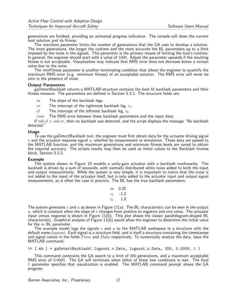
Algorithm The dead-zone characteristic DZ(·) is described as

u(t) = N(v(t)) = DZ(v(t)) =

mr(v(t)− br) if v(t) ≥ br0 if bl < v(t) < brml(v(t)− bl) if v(t) ≤ bl,

(22)

where mr > 0, ml > 0, br > 0, and bl < 0 (see Figure 17).

Figure 17: Dead-zone Characteristic

The parametrized model of the dead-zone nonlinearity can be unified as

u(t) = N(v(t)) = N(θ∗; v(t)) = −θ∗Tω∗(t) + a∗s(t) (23)

Introducing the indicator function χ[X] of the event X as

χ[X] =

{1 if X is true,0 otherwise,

(24)

we define the dead-zone indicator functions

χr(t) = χ[u(t) > 0], (25)

χl(t) = χ[u(t) < 0]. (26)

Then, introducing the dead-zone parameter vector and its regressor,

θ∗ = [mr,mrbr,ml,mlbl]T , (27)

ω∗(t) = [−χr(t)v(t), χr(t),−χl(t)v(t), χl(t)]T , (28)

we obtain the desired form (23) with a∗s(t) = 0 for the dead-zone characteristic (22).



Dead-zone inverse. Let the estimates of the dead-zone parameters mrbr, mr, mlbl, ml be mrbr,

mr, mlbl, ml, respectively. Then the inverse for the dead-zone characteristic is described by

v(t) = NI(ud(t)) = DI(ud(t)) =

ud(t)+mrbr

mrif ud(t) > 0,

0 if ud(t) = 0,ud(t)+mlbl

mlif ud(t) < 0.

(29)

For the dead-zone inverse to arrive at the desired form, we introduce the inverse indicator functions

χr(t) = χ[v(t) > 0], (30)

χl(t) = χ[v(t) < 0] (31)

and the inverse parameter vector and regressor

θ = [mr, mrbr, ml, mlbl]T , (32)

ω(t) = [−χr(t)v(t), χr(t),−χl(t)v(t), χl(t)]T . (33)

Then, the dead-zone inverse is

ud(t) = mrχr(t)v(t)− mrbrχr(t) + mlχl(t)v(t)− mlblχl(t)

= −θTω(t). (34)

Input Signals

r The input signal to the actuator’s controller (e.g. pilot stick input).ud The desired signal input to an ideal (i.e. no dead-zone) actuator that would achieve the

response dictated by the reference signal, r.y The measured system response to the actuator control.

Output Signals


theta The adapting nonlinear inverse parameters, in an internal form.slopeIntercept The adapting nonlinear inverse parameters, [ml, bl,mr, cr].




Figure 18: Dead-zone Inverse Simulink Block Parameters

Transfer Function Type Selects the form for expressing the system dynamics. The param-eters dialog will adjust to show all parameters required by the cho-sen transfer function type, which is one of state-space, polynomial, orzero/pole/gain.

Initial Values A vector of the initial values for the dead-zone parameters,[ml0, bl0,mr0, bl0].

Minimum Bounding Values A 4-element vector of the minimum bounds for the dead-zone parame-ters, [mlmin, blmin,mrmin, brmin].

Maximum Bounding Values A 4-element vector of the maximum bounds for the dead-zone parame-ters, [mlmax, blmax,mrmax, brmax].

NI Gains A 4-element vector of the gains (Γ) controlling the dead-zone parameteradaptation, [Γml,Γbl,Γmr,Γbr].

UsageThe DI components are applicable to continuous- and discrete-time single-input / single-output

(SISO) systems driven by actuators containing dead-zone, and having measurable system output, y.The generalized feedback control system is shown in Figure 2.

The engineer will design a controller (C1) to generate the idealized actuator control signal (ud)as though the actuator did not exhibit dead-zone. This control signal will feed into the DI block, becompensated and produce the actuator driving signal (v) to achieve the required response.

5.3.6 Dead-zone Parameter ID

DescriptionThe AIFAC toolbox’s genetic algorithm (GA)-based dead-zone (gaDetectDeadzone) detection tool is

designed to help the engineer identify the dead-zone nonlinearity and its parameters from data, whetherit be measurement data or simulation output. In Figure 2, the block N(·) represents the nonlinear



actuator. The tool accepts as input the actuator driving signal v and the actuator response signal u(Figure 2). It produces figures showing the actuator’s input-versus-output characteristics, estimates ofthe nonlinearity’s parameters, and a measure of the actuator’s response fitted to the nonlinearity.

A most compelling capability of the GA technique is its accuracy in the presence of random measure-ment noise. The engineer need not measure or remove the noise from the data. Unlike calculus-basedsearch techniques, GA methods generally do not get “fooled” by local optima. Whereas traditionalsearch methods parse the data to identify parameters, a GA estimates parameters and then comparesthe solution against the data. Thus, the GA tolerates the noise because the GA is evaluating an idealnonlinearity with the candidate parameters against the measured system data, and searches for the“best” fit, not a perfect fit.

The gaDetectDeadzone tool has the following MATLAB syntax:

[ mb ] = gaDetectDeadzone( v, u, maxGens, minFitness, visualize )

Algorithm A genetic algorithm (GA) is a global search heuristic technique that seeks to find an exactor approximate solution by using stochastic processes to “evolve” to the solution. One application ofGA is curve fitting, and the AIFAC toolbox uses GA to fit ideal dead-zone (DZ) and backlash (BL)characteristics to measured actuator data.

The most fundamental element of a GA is a “gene”, which is a representation of part of a solution.One or more genes are combined to form a “chromosome”, which represents a solution. In this toolbox,a gene is a parameter of the ideal DZ or BL characteristic. The GA begins by randomly generatingan initial population (i.e. set) of candidate solutions, which comprise generation 0. This generation isevaluated and sorted based on each chromosome’s “fitness”. Fitness is a measure of the optimality ofthe solution. In this application, fitness is the RMS error between the ideal curve, represented by thecandidate solution, and the measured actuator response. The GA then enters the select-mutate-evaluateloop.

The loop first randomly selects candidates from generation i, where the fittest candidates are morelikely to be selected than the less fit candidates, and adds the selected candidates to generation i+ 1.The selected candidates each mate with a partner from the candidate pool, and through an operationknown as crossover, swap their genes at a certain point and create two offspring, each of which containparts of their parents chromosomes. The next step is to randomly mutate the genes of each generationi+ 1 candidate, adding the mutated chromosome back into generation i+ 1. Finally, generation i+ 1 isevaluated, sorted, and trimmed to a fixed population size. The loop termination criteria are evaluated,and the loop exits or operates on i+ 1. The loop termination criteria are a maximum number of loops,or a solution whose RMS error is less than or equal to a given value.

Input Parameters

v The actuator input signal.u The actuator response signal.maxGens The maximum number of generations to evaluate (must be greater than 0.0).minFitness The minimum fitness measure required of an acceptable solution (must be pos-

itive).visualize The visualization flag. If the flag is non-zero, the tool will plot and display

intermediate generations.The visualize parameter enables and disables the algorithm’s progress display. When visualization

is enabled, the tool outputs its progress to a MATLAB figure and the console every 1/20 of maxGens.The figure will plot the DZ characteristic of the current best solution. The figure will update as thegenerations are finished, providing an animated progress indication. The console will show the currentbest solution and its fitness.

The maxGens parameter limits the number of generations that the GA uses to develop a solution.The more generations, the longer the runtime and the more accurate the DZ parameters up to a limitimposed by the noise in the signals. This parameter is the primary means of limiting the tool’s runtime.In general, the engineer should start with a value of 1000. Adjust the parameter upwards if the resulting



fitness is not acceptable. Visualization may indicate that RMS error does not decrease below a certainvalue due to the noise.

The minFitness parameter is another terminating condition that allows the engineer to quantify themaximum RMS error (e.g. minimum fitness) of an acceptable solution. The RMS error will never bezero in the presence of noise.

Output ParametersgaDetectDeadzone returns a MATLAB structure contains the best fit dead-zone parameters and

their fitness measure. The parameters are defined in Section 5.3.5. The structure fields are:

ml The slope of the leftmost dead-zone characteristic, ml.bl The intercept of the leftmost dead-zone characteristic, bl.mr The slope of the rightmost dead-zone characteristic, mr.cr The intercept of the rightmost dead-zone characteristic, br.rms The RMS error between these dead-zone parameters and the input data.

UsageTo use the gaDetectDeadzone tool, the engineer must first obtain data for the actuator driving

signal v and the actuator response signal u, whether by measurement or simulation. These data arepassed to the MATLAB function, and the maximum generations and minimum fitness levels are variedto obtain the required accuracy. The scripts results may then be used as initial values to the DeadzoneInverse block, Section 5.3.5.

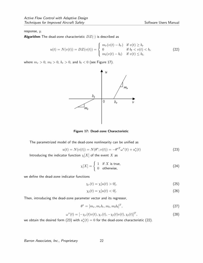
ExampleThe system shown in Figure 5.3.6 models a unity-gain actuator with a dead-zone nonlinearity. The

dead-zone is driven by a sum of sinusoids, with normally distributed white noise added to both the inputand output measurements. While the system is very simple, it is important to notice that the noise isnot added to the input of the actuator itself, but is only added to the actuator input and output signalmeasurements, as is often the case in practice. The DZ has the true dead-zone parameters:

ml 6.5bl -1.1mr 0.7br 0.2

Figure 19: Dead-zone Model Example



The system generates v and u as shown in Figure 20(a). The DZ characteristic can be seen in theoutput u, which is zero plus some noise, when bl < v < br. The actuator input versus response is shownin Figure 20(b). This plot shows the classic DZ characteristic. Graphical analysis of these plots wouldallow the engineer to determine initial values for the DZ parameters.

(a) Actuator input v and output u (b) Actuator response v vs u

Figure 20: Dead-zone Model Input-Output

The example model logs the signals v and u to the MATLAB workspace in a structure with thedefault name logsout. Each signal is a structure field, and is itself a structure containing the timestampsand signal values in the fields Time and Data respectively. To numerically analyze the data, issue theMATLAB command:

>> [ mb ] = gaDetectDeadzone( logsout.v.Data, logsout.u.Data, 1000, 0.05, 1 )

This command constrains the GA search to a limit of 1000 generations, and a maximum acceptableRMS error of 0.05. The GA will terminate when the either of these two conditions is met. The final1 parameter specifies that visualization is enabled. The MATLAB command prompt shows the GAprogress:

Gen RMS ml bl mr br1 3.8083 0.8578 -0.0890 0.6888 0.911351 3.2499 1.3226 -0.0542 0.5993 0.5099101 2.7452 1.7366 0.0432 0.5380 0.5246151 2.3082 2.0488 0.3109 0.6007 0.4605201 1.9937 2.4798 0.2507 0.6582 0.4607251 1.7893 2.8661 0.1432 0.7127 0.4518301 1.6195 3.1350 -0.0669 0.7655 0.4447351 1.4233 3.4925 -0.2549 0.7579 0.4457401 1.2148 3.9167 -0.4020 0.6990 0.3678451 1.0064 4.2972 -0.6125 0.7873 0.4280501 0.8241 4.6888 -0.7074 0.8694 0.4845551 0.6344 5.1007 -0.7902 0.7891 0.4037601 0.4645 5.4775 -0.8834 0.7604 0.4507651 0.3052 5.8246 -0.9808 0.7701 0.4378701 0.1613 6.1635 -1.0418 0.7701 0.3347751 0.0676 6.4348 -1.0807 0.7492 0.3127

mb =



ml: 6.4659bl: -1.0888mr: 0.7127br: 0.2117

rms: 0.0496

The results show the evolution of the parameters, and the final results. Notice that the bl starts outnegative, evolves to a positive value, and the reverses direction to converge to −1.0888, which is veryclose to the true −1.1. This result demonstrates that the GA may identify false solutions in the shortterm, but will converge to a correct solution if correctly designed and left to evolve. It also cautionsthe user against using too few generations. As shown, if the maximum number of generations had been150, the bl parameter would have been about 0.3109, which is the worst parameter estimate. Again,the DI block would eventually adapt and converge to the true parameters, but would take longer giventhe poor initial estimate.

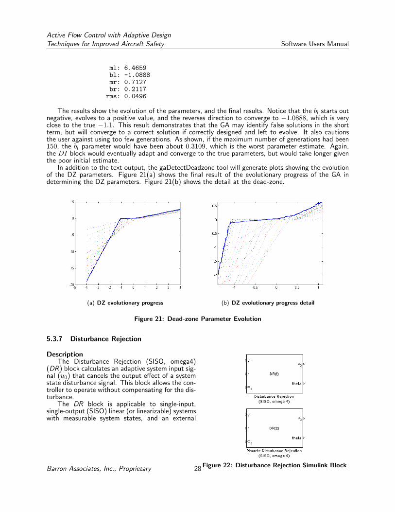
In addition to the text output, the gaDetectDeadzone tool will generate plots showing the evolutionof the DZ parameters. Figure 21(a) shows the final result of the evolutionary progress of the GA indetermining the DZ parameters. Figure 21(b) shows the detail at the dead-zone.

(a) DZ evolutionary progress (b) DZ evolutionary progress detail

Figure 21: Dead-zone Parameter Evolution

5.3.7 Disturbance Rejection

Description

Figure 22: Disturbance Rejection Simulink Block

The Disturbance Rejection (SISO, omega4)(DR) block calculates an adaptive system input sig-nal (u0) that cancels the output effect of a systemstate disturbance signal. This block allows the con-troller to operate without compensating for the dis-turbance.

The DR block is applicable to single-input,single-output (SISO) linear (or linearizable) systemswith measurable system states, and an external



state disturbance signal.

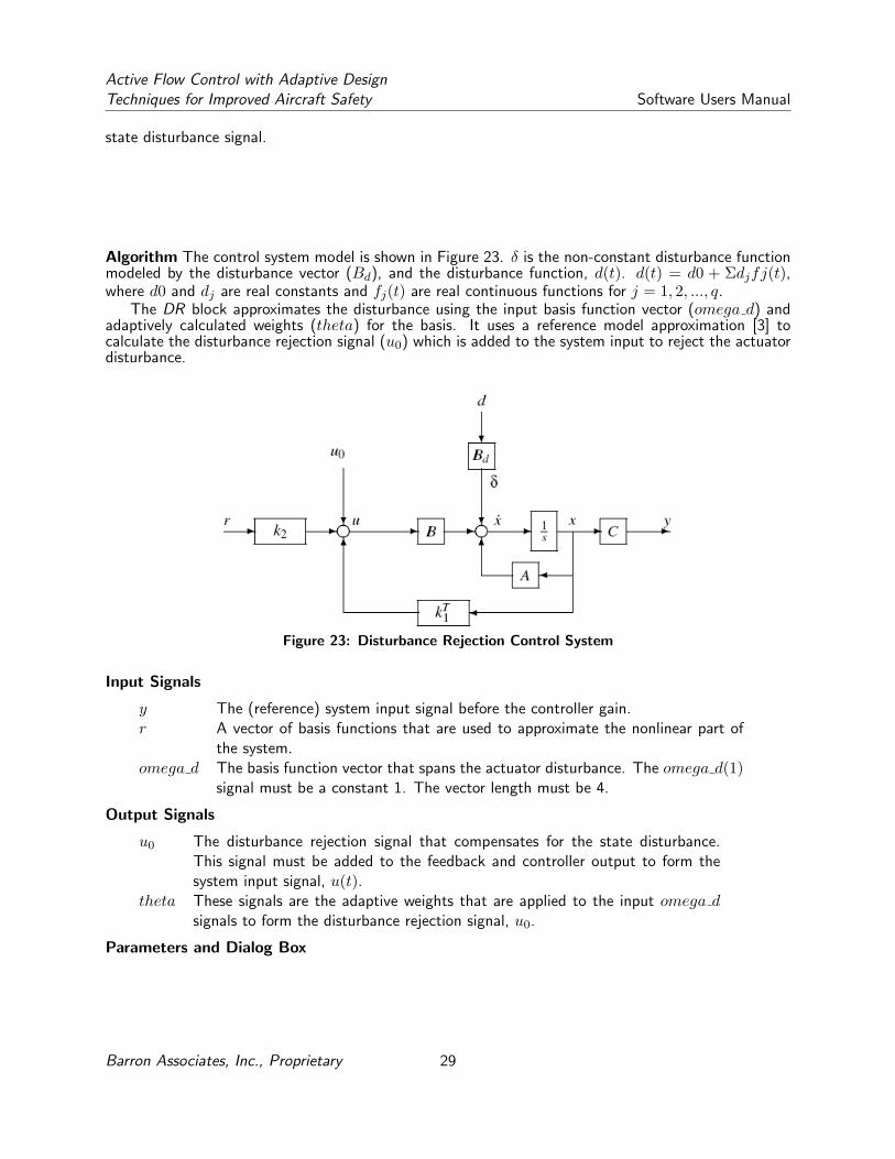
Algorithm The control system model is shown in Figure 23. δ is the non-constant disturbance functionmodeled by the disturbance vector (Bd), and the disturbance function, d(t). d(t) = d0 + Σdjfj(t),where d0 and dj are real constants and fj(t) are real continuous functions for j = 1, 2, ..., q.

The DR block approximates the disturbance using the input basis function vector (omega d) andadaptively calculated weights (theta) for the basis. It uses a reference model approximation [3] tocalculate the disturbance rejection signal (u0) which is added to the system input to reject the actuatordisturbance.

Figure 23: Disturbance Rejection Control System

Input Signals

y The (reference) system input signal before the controller gain.r A vector of basis functions that are used to approximate the nonlinear part of

the system.omega d The basis function vector that spans the actuator disturbance. The omega d(1)

signal must be a constant 1. The vector length must be 4.

Output Signals

u0 The disturbance rejection signal that compensates for the state disturbance.This signal must be added to the feedback and controller output to form thesystem input signal, u(t).

theta These signals are the adaptive weights that are applied to the input omega dsignals to form the disturbance rejection signal, u0.




Figure 24: Disturbance Rejection Simulink Block Parameters

k2 The input gain for the nominal system controller.gamma1 The gain vector for adapting the disturbance rejection parameters. This

column vector has the same number of elements as the omega d inputsignal.

theta(0) The initial values for the adaptive disturbance rejection parameters,theta. This column vector has the same number of elements as thetheta output signal.

Transfer Function Type Selects the form for expressing the system reference model. The ref-erence model transfer function must have no zeros (i.e. numerator =1). The denominator must be a monic polynomial of the same rela-tive degree as the system, and must have all roots in the left half-plane.The parameters dialog will adjust to show all parameters required by thechosen transfer function type, and the Numerator and Zeros parameterswill be disabled and forced to the required value, 1.

UsageTo use the DR component, the system must be a SISO, linear (or linearizable) system with mea-

surable system states. Create a disturbance model to develop the disturbance signal spanning functions(omega d). Add the disturbance rejection signal (u0) to the system input signal (u) to drive the system.



Typically, the adaptive weights (theta) output signal will be saved to the MATLAB workspaceduring simulation, and the final results used as the initial condition parameter theta(0) to ensure thatthe deployed system starts execution with an accurate initial state.

ExampleIn example shown in Figure 25 is an aircraft, where the state variables in x(t) are the lateral velocity

x1(t), roll rate x2(t), yaw rate x3(t), and roll angle x4(t). The input u(t) is used to control a syntheticjet actuator to change the output y(t) = x4(t), or the roll angle. The system has an actuationdisturbance d(t) = Bdd(t). The transfer function has relative degree 2, so the chosen reference modelis 1

s2+2s+2. The disturbance signal is a sum of high-frequency sinusoids.

Figure 25: Disturbance Rejection Example Model

The disturbance and disturbance rejection signals are applied to the system states as shown in Figure26.



Figure 26: Disturbance Rejection Example System Model

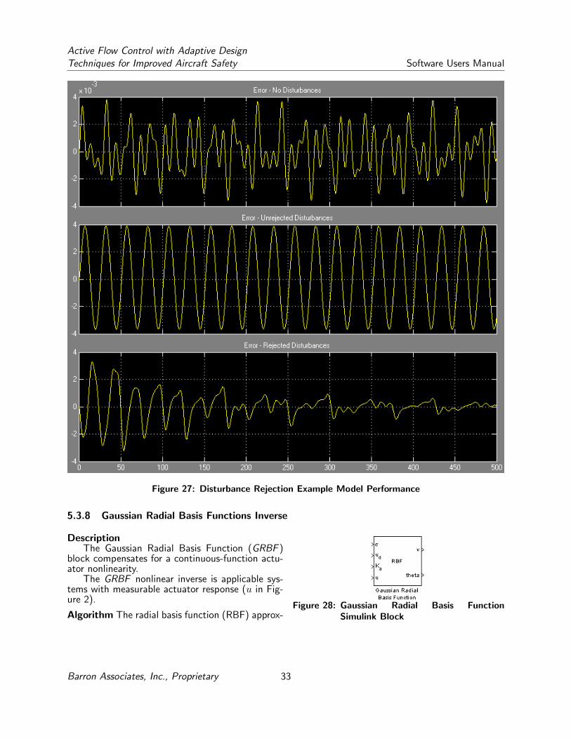
Three system responses are plotted in Figure 27: no disturbance, unrejected disturbance, and rejecteddisturbance. The error signals are the differences in the system response and the reference model systemresponse. The system with rejected disturbance shows a decaying error due to the DR component’sadaptive rejection of the disturbance signal.



Figure 27: Disturbance Rejection Example Model Performance

5.3.8 Gaussian Radial Basis Functions Inverse

Description

Figure 28: Gaussian Radial Basis FunctionSimulink Block

The Gaussian Radial Basis Function (GRBF )block compensates for a continuous-function actu-ator nonlinearity.

The GRBF nonlinear inverse is applicable sys-tems with measurable actuator response (u in Fig-ure 2).

Algorithm The radial basis function (RBF) approx-



imator is defined as

f(x) =N∑i=1

θig(‖x − ci‖) (35)

where x ∈ <n, {ci}Ni=1 are a set of center locations, ‖x − ci‖ is the distance from the evaluation pointto the i-th center, and g(·) : <+ → <1 is a radial function. One of the most common g(·) functions isa Gaussian:

g(x) = σe−πσ2(x−ci)2 (36)

where σ is the standard deviation of the basis function.The GRBF block approximates a nonlinearity as a sum of weighted Gaussian RBF. The RBF sum

may be thought of as a Fourier series where the sine and cosine functions are replaced by Gaussianfunctions. Each curve in the sum is centered about a point in the nonlinearity’s range. The figure showsa set of three Gaussian functions (σ = 0.2) that are evenly spaced at −3.0, 1.0, and 4.0. Both thenumber of basis functions, their standard deviations, and their centers are block parameters to be tunedfor the application.

This block uses feedback to adaptively estimate the basis function weights, and compensates theactuator input command signal so that the actuator will achieve desired response.

Figure 29: Gaussian Radial Basis Functions

Input Signals

σ The standard deviation of the Gaussian basis functions.ud A signal proportional to the desired actuator response.Ka The gain applied when adjusting the RBF weights.u The measured actuator response signal.

Output Signals


theta The adapting nonlinear inverse parameters, in an internal form.




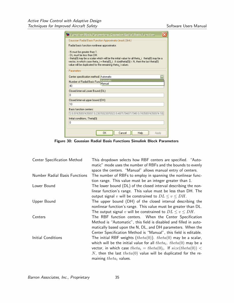
Figure 30: Gaussian Radial Basis Functions Simulink Block Parameters

Center Specification Method This dropdown selects how RBF centers are specified. “Auto-matic” mode uses the number of RBFs and the bounds to evenlyspace the centers. “Manual” allows manual entry of centers.

Number Radial Basis Functions The number of RBFs to employ in spanning the nonlinear func-tion range. This value must be an integer greater than 1.

Lower Bound The lower bound (DL) of the closed interval describing the non-linear function’s range. This value must be less than DH. Theoutput signal v will be constrained to DL ≤ v ≤ DH.

Upper Bound The upper bound (DH) of the closed interval describing thenonlinear function’s range. This value must be greater than DL.The output signal v will be constrained to DL ≤ v ≤ DH.

Centers The RBF function centers. When the Center SpecificationMethod is “Automatic”, this field is disabled and filled in auto-matically based upon the N, DL, and DH parameters. When theCenter Specification Method is “Manual”, this field is editable.

Initial Conditions The initial RBF weights (theta(0)). theta(0) may be a scalar,which will be the initial value for all thetai. theta(0) may be avector, in which case thetai = theta(0)i. If size(theta(0)) <N , then the last theta(0) value will be duplicated for the re-maining thetai values.



UsageTo use the GRBF component, the system must be SISO where the actuator response (u) is measur-

able. The engineer must choose RBF parameters to adequately compensate for the nonlinearity whilenot overfitting the response. The runtime of the component increases as the number of RBF functions,which require the exponential, a relatively expensive function.

During simulation, the output signal theta may be directed to a MATLAB Workspace block and thefinal results used as the initial conditions for the next run and/or deployment. This technique increasesthe adaptive weights’ accuracy at t = 0.

ExampleThe GRBF component was tested in the system shown in Figure 31. The input signal (ud) is a

sum of sinusoids. The nonlinear component is a high angle-of-attack model of the synthetic jet:

u(t) = 15.0 − 10.01 + v(t)

. (37)

Figure 31: Gaussian RBF Test Harness

The relevant input (ud) and outputs (u) are displayed in Simulink scopes for real-time analysis, andsaved in the MATLAB workspace for offline analysis.

The performance is shown in Figure 32. Figure 32(a) shows the actuator’s desired response (ud)and actual response (u) for the adaptive gain Ka = 0.001. The error is small enough that Figure 32(b)is necessary to visualize it. The GRBF adapts quickly, so a very small gain is necessary to see anyappreciable error. Figure 33 shows that increasing Ka from 0.001 to 0.1 decreases the error appreciably.



(a) GRBF Test Results (b) GRBF Test Results Detail

Figure 32: Gaussian RBF Test Results (Ka = 0.001)

(a) GRBF Error (Ka = 0.001) (b) GRBF Error (Ka = 0.1)

Figure 33: Gaussian RBF Test Error



5.3.9 Taylor Series Inverse

Description

Figure 34: Taylor Series Simulink Block

The Taylor Series (TS) Nonlinear Adaptive In-verse block compensates for a continuous-functionactuator nonlinearity. The block approximates anonlinearity using an n-order Taylor Series to ap-proximate a nonlinearity which is a function of twovariables, that is N(ud, alpha).

The TS approximator applies to a single-input,single-output (SISO) system with a measurable sys-tem response, y.

This block uses feedback to adaptively estimatethe Taylor term coefficients, and compensates theactuator input command signal so that the actuatorwill achieve desired response without directly com-pensating for the nonlinearity in the control law.

Input Signals

v The actuator driving signal.ud A signal proportional to the desired actuator response.alpha The aircraft angle of attack.e(t) The system error signal defined as the difference between the system reference

input and the system response.

Output Signals


thetaa The adapting nonlinear inverse parameters, in an internal form.thetac The adapting nonlinear inverse parameters, in an internal form.




Figure 35: Taylor Series Simulink Block Parameters

M Degree The Taylor Series degree. The number of TS terms is N = (M + 1)(R +1),where 0 ≤M ≤ 9.

R Degree The Taylor Series degree. The number of TS terms is N = (M + 1)(R +1),where 0 ≤ R ≤ 9.

a The point in the range of v about which the TS is being estimated.b The point in the range of alpha about which the TS is being estimated.c The point in the range of u about which the TS is being estimated.Gamma1 The adaptive estimate gain for thetaa. This value may be a scalar, or an N×N

vector, where N is the number of TS terms.thetaa(0) The initial estimate for thetaa. This value must be an N × 1 vector, where N

is the number of TS terms.thetaaLowerBound The lower bound of the closed interval containing the thetaa estimates. This

value must be an N × 1 vector, where N is the number of TS terms.thetaaUpperBound The upper bound of the closed interval containing the thetaa estimates. This

value must be an N × 1 vector, where N is the number of TS terms.Gamma2 The adaptive estimate gain for thetac. This value may be a scalar, or an N×N

vector, where N is the number of TS terms.



thetac(0) The initial estimate for thetac. This value must be an N × 1 vector, where Nis the number of TS terms.

thetacLowerBound The lower bound of the closed interval containing the thetac estimates. Thisvalue must be an N × 1 vector, where N is the number of TS terms.

thetacUpperBound The lower bound of the closed interval containing the thetac estimates. Thisvalue must be an N × 1 vector, where N is the number of TS terms.

5.4 Related Processing

This section is not applicable to AIFAC.

5.5 Data Backup


5.6 Recovery from Errors, Malfunctions, and Emergencies


5.7 Messages


5.8 Quick-Reference Guide


6 Notes

6.1 Abbreviations and Acronyms

AIFAC Adaptive Inverse For Actuator CompensationANN3NI Adaptive Neural Network (3-Layer) Nonlinear InverseBI Backlash InverseCSCI Computer Software Configuration ItemDR Disturbance RejectionDZ Dead-zoneGA Genetic AlgorithmGRBF Gaussian Radial Basis FunctionN NonlinearNI Nonlinear InverseRBF Radial Basis FunctionRMS Root Mean SquareSISO Single-Input, Single-OutputSUM Software Users ManualTS Taylor Series


ACTIVE FLOW CONTROL WITH ADAPTIVE ... - Barron …€¦ · The AIFAC toolbox provides advanced...

Documents

Transcript of ACTIVE FLOW CONTROL WITH ADAPTIVE ... - Barron …€¦ · The AIFAC toolbox provides advanced...