Vertical Integration and Competition

8/8/2019 Vertical Integration and Competition

http://slidepdf.com/reader/full/vertical-integration-and-competition 1/16

THE U-SHAPED R ELATIONSHIP BETWEEN

VERTICAL I NTEGRATION AND COMPETITION:THEORY AND EVIDENCE

Philippe Aghion Rachel Griffith

Peter Howitt



The U-Shaped Relationship Between Vertical

Integration and Competition: Theory and

Evidence∗

Philippe Aghion†, Rachel Griffith‡, and Peter Howitt§

June 12, 2006

Abstract

This paper considers how competition can aff ect aggregate innovativeactivity through its eff ects on firms’ decision whether or not to verticallyintegrate. A moderate increase in competition enhances innovation incen-tives, too much competition discourages innovative eff ort. These eff ectsgenerates an inverted-U relationship between competition and innovationand between competition and the incentive to vertically integrate. Pre-liminary evidence finds that there is a non-linear relationship betweencompetition and the propensity of firms to vertically integrate. These re-

sults seem to be more consistent with the Property Right Theory (PRT)of vertical integration than with the Transaction Cost Economics (TCE)approach.

1 Introduction

In previous work (see Aghion et al (2005)), we pointed to the existence of aninverted-U shaped relationship between competition and innovation. Our expla-

nation for this relationship would emphasize the ”composition eff

ect” competi-tion has on the steady-state distribution of technological gaps across industries.The present paper is part of an attempt at analyzing how competition can af-fect aggregate innovative activity through its eff ects on firms’ organization. Ourfocus is on firms’ decision whether or not to vertically integrate, with the fol-lowing driving intuition: a moderate increase in product market competition,by improving the outside options of a non-integrated supplier, will enhance her



to also innovate more. However, too much competition on the producer’s mar-ket will end up discouraging the producer’s eff ort in a non-integrated firm, astoo much of the innovation surplus will then accrue to the supplier. This againgenerates an inverted-U relationship between competition and innovation, butwhich is mirrored by a similar relationship between competition and the incen-tive to vertically integrate.

Showing the existence of an inverted-U relationship between competition andvertical integration sheds light on the debate between those who believe morein the “Transaction Cost Economics” (TCE) approach to vertical integration,pioneered by Williamson (1975, 1985), and those who support the “PropertyRight Theory” (PRT) approach, developed by Grossman-Hart (1986) and Hart-Moore (1990).1 According to the TCE approach, vertical integration is a wayfor contracting parties involved in a specific-relationship to limit ex post bar-gaining inefficiencies due to hold-up, and thereby minimize the loss in ex anteinvestment that would result from it. This approach thus predicts a positive

correlation betwen vertical integration and the degree of relation specificity. Ac-cording to the PRT approach, the ownership structure will aff ect not so muchthe ex post bargaining efficiency but rather the relative bargaining powers of the(two) contracting parties, and therefore their relative ex ante investment incen-tives. Thus, while vertical integration should enhance both parties’ investmentspositively in the TCE approach, by reducing the extent of ex post inefficiency,in the PRT approach ownership by one party, say the buyer, will enhance thebuyer’s ex ante incentives at the expense of the seller’s ex ante incentives, as itenhances the buyer’s bargaining power ex post at the expense of the seller’s bar-

gaining power.2 Thus the TCE approach predicts that increased competition onthe producer’s (or supplier’s) market, which reduces the overall degree of assetspecificity, should therefore reduce the need for vertical integration in order topreserve ex ante investment incentives by either party. On the other hand, asalready suggested by our discussion above, and as we show more formally inSection 2 below, the PRT approach predicts a U-shaped relationship betweenvertical integration and competition on the producer’s market. In Section 3we argue that this U-shaped pattern is supported by the empirical analysis of vertical integration and entry using UK cross-firm panel data.

1 A first attempt at deriving distinguishing testable implications of the two approaches, isby Whinston (2001).

2 An attempt at using cross-industry micro panel data to tell these two theories apart wasmade in Acemoglu-Aghion-Griffith-Zilibotti (2005). Using technology intensity to measurerelationship-specific investments, they look at the relationship between pairs of supplying andproducing industries, and show that, as predicted by the PRT approach, (backward) verticalintegration - that is, producer ownership - is significantly correlated with the investment



2 Basic framework

2.1 Production and ex post bargaining

We consider an economy composed of individuals with risk-neutral preferencesfor consumption. A final good is produced with a continuum of intermediateinputs according to:

y =Z 10

xαi

di, (1)

where α ∈ (0, 1).In each sector i, the incumbent producer produces her intermediate good

according to:xi = f (zi, si), (2)

where zi is the input of general good used as capital into the production of intermediate input, and si is the input of a specialized good, used only in sector

i, and available in supply equal to one.The production function for intermediate input satisfies:

f (zi, si) =

½zi if si ≥ 10 otherwise

.

Thus the specialized input si is indispensable to the production of intermediategood i.

Although she enjoys monopoly power, intermediate good producer i faces a

competitive fringe of firms that can produce the same intermediate good but athigher unit cost. More precisely, potential imitators can produce according tothe technology

f m(zi, si) =

½zi

aif si ≥ 1

0 otherwise,

where a > 1 measures the degree of product market competition in the interme-diate input market, with lower a (that is, closer to 1) corresponding to a higherdegree of competition.

If the incumbentfi

rm (call him “the entrepreneur”) in sector i manages toobtain the services of the specialized input producer (call him “the manager”)in that sector, she does not face any eff ective competition, since potential im-itators then do not have access to the specialized input. The incumbent firmcan then sell her intermediate good to the final sector at the unconstrainedmonopoly price, which is equal to the marginal product of the intermediategood in producing the final good,



wherexi = f (zi, 1) = zi.

Equivalently therefore, the intermediate producer will choose xi to

maxxi

{αxαi− xi} = πi,

which in turn, by first-order conditions, immediately yields:

πi =1− α

αα

2

1−α = π.

To determine how this surplus is divided between the intermediate entre-preneur and the manager, we need to compute what the manager would obtainif he sold his specialized input to imitators. The answer is that, if the fringeof imitators is competitive, the manager should get the whole surplus πm

ifrom

selling his input to an imitator. That surplus, in turn, is determined by thesame maximization program as above, except that the production function f is

replaced by f m, namely:

πm

i = maxzi

{ pif m(zi, 1)− zi}

where nowxi = f m(zi, 1),

or equivalentlymaxxi

{αxαi− axi}.

This immediately yieldsπmi =

πχ

whereχ = a

α

1−α

also measures product market competition.Now, we can easily determine the outcome of ex post bargaining between

the intermediate producer (or entrepreneur) and the specialized input supplier(or manager) in each intermediate sector i.

First, if a competitive fringe of imitators shows up, the manager can secureπmi

by defecting to an imitator. Assuming that the incumbent entrepreneurmakes a take-it-or-leave it off er to the manager ex post, she will concede πm

ito

the manager to secure his specialized input, so that the entrepreneur’s ex postresidual payoff is simply equal to

πi πm = π(11

)



Here we implicitly assume that

χ < 2

so that the outside option of the manager moving to the imitator is actuallybinding.

2.2 Ex ante investments

We assume that the incumbent firm in any sector i must invest in R&D inorder to innovate. Innovation, in turn, creates the profit opportunity π. Letd(z) denote the R&D cost of innovating with probability z, and assume that

d(z) =zu1

u1

,

where u1 > 1.Once a new technology has been invented by the incumbent producer, themanager must create a suitable input or component for that new technology,and we let c(e) denote the manager’s cost of generating such a component withprobability e. We let:

c(e) =eu2

u2

,

where u2 > 1.

2.3 Timing of events

At the beginning of a period the incumbent producer in any sector invests inquality-enhancing innovation. If she successfully innovates, then she turns to thespecialized input supplier in that sector for him to come up with a componentwhich is adapted to the new technology. Then a competitive fringe of potentialimitators on the intermediate market show up with probability η > 0. Whetherthe fringe shows up or not, if the component is successfully produced, then theentrepreneur and the manager bargain over the surplus. Otherwise they both

get zero profits, as the previous technology keeps prevailing in that intermediatesector.

3 Imitation, competition, and the choice between

integration and non-integration



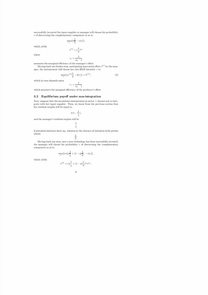
successfully invented the input supplier or manager will choose his probabilitye of discovering the complementary component so as to

maxe

{eπ

2− c(e)},

which yields

eV I = (π

2)ε2

where

ε2 =1

u2 − 1

measures the marginal efficiency of the manager’s eff ort.Moving back one further step, anticipating innovation eff ort eV I by the man-

ager, the entrepreneur will choose her own R&D intensity z to

maxz

{zeV I π

2

− d(z)} = U V I , (3)

which in turn depends upon

ε1 =1

u1 − 1

which measures the marginal efficiency of the producer’s eff ort.

3.2 Equilibrium payoff under non-integration

Now, suppose that the incumbent entrepreneur in sector i chooses not to inte-grate with her input supplier. Then, we know from the previous section thather residual surplus will be equal to

π(1−1

χ),

and the manager’s residual surplus will be

π

χ

if potential imitators show up, whereas in the absence of imitation both partiesobtain

π

2.

Moving back one step, once a new technology has been successfully inventedthe manager will choose his probability e of discovering the complementary



which is greater than eV I whenever the competitive fringe is binding, that isχ < 2.

Note that the case where imitation never occurs (that is, when η = 0) isidentical to the case under vertical integration, which is not surprising since ineither case the manager has no outside option.

Moving back one further step, anticipating innovation eff ort eNI by themanager, the entrepreneur will choose her own R&D intensity z to

maxz

{zeNI (η(1−1

χ) + (1 − η)

1

2)π − d(z)} = U NI . (4)

3.3 Imitation and vertical integration

Comparing between (3) and (4), we can establish:

Lemma 1 The di ff erence U NI − U V I either always decreases, or always in-

creases, or fi rst increases and then decreases as the probability of imitation ηincreases from zero to one.

Proof. Consider the function

ν (η) = (η1

χ+ (1− η)

1

2)ε2(η(1−

1

χ) + (1 − η)

1

2). (5)

Once we fully spell out the expressions for (3) and (4), all we need to showis that ν is either increasing, or decreasing, or inverted-U shaped in η. To this

eff ect, let us calculate the derivative ν 0

(η). We have:

ν 0(η) = (1

χ−

1

2)(η

1

χ+ (1− η)

1

2)ε2−1[

ε2 − 1

2− η(ε2 + 1)(

1

χ−

1

2)].

If ν was U-shaped, we would have:

ν 0(0) < 0 < ν 0(1)

or equivalently

ε2 − 12

< 0 < ε2 − 12

− (ε2 + 1)( 1χ− 1

2).

But this cannot be since1

χ>

1

2

by assumption. This establishes the lemma.



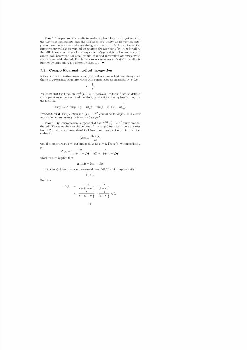
Proof. The proposition results immediately from Lemma 1 together withthe fact that investments and the entrepreneur’s utility under vertical inte-gration are the same as under non-integration and η = 0. In particular, theentrepreneur will choose vertical integration always when ν 0(η) < 0 for all η,she will choose non integration always when ν 0(η) > 0 for all η, and she willchoose non-integration for small values of η and integration otherwise whenν (η) is inverted-U shaped. This latter case occurs when ε2ν 0(η) < 0 for all η issufficiently large and χ is sufficiently close to 1.

3.4 Competition and vertical integration

Let us now fix the imitation (or entry) probability η but look at how the optimalchoice of governance structure varies with competition as measured by χ. Let

x =1

χ.

We know that the function U NI (x) − U V I behaves like the ν -function definedin the previous subsection, and therefore, using (5) and taking logarithms, likethe function:

ln ν (x) = ε2 ln(ηx + (1− η)1

2) + ln(η(1− x) + (1 − η)

1

2).

Proposition 3 The function U NI (x) − U V I cannot be U-shaped: it is either

increasing, or decreasing, or inverted-U shaped.

Proof. By contradiction, suppose that the U NI (x) − U V I curve was U-shaped. The same then would be true of the ln ν (x) function, where x variesfrom 1/2 (minimum competition) to 1 (maximum competition). But then thederivative

∆(x) =d ln ν (x)

dx

would be negative at x = 1/2 and positive at x = 1. From (5) we immediatelyget:

∆

(x

) =

ε2η

ηx + (1− η)12−

η

η(1− x) + (1− η)12,

which in turn implies that

∆(1/2) = 2(ε2 − 1)η.

If the ln ν (x) was U-shaped, we would have ∆(1/2) < 0 or equivalently:



which in turn implies that ln ν (x) is not U-shaped. This contradiction estab-lishes the proposition.

4 Empirical evidence

We are interested in investigating whether the propensity for firms to vertically

integrate varies systematically with the extent of competition in the productmarket, and if so whether it does so in ways that are consistent with the TCEview of vertical integration or the PRT view. Recall that under the formerwe would expect vertical integration to decline as competition increases. Incontrast, Proposition 3 states that under the PRT as competition increasesthe probability of vertical integration could follow this pattern, but could alsoincrease or initially decrease and then increase.

We look at how the probability of a producer and supplier being verticallyintegrated varies with several simple measure of competition. We should em-

phasize that what we are capturing here is a correlation, and not a causalrelationship.

4.1 Data

We use a large nationally representative data set on all UK manufacturingplants3 over a thirteen year period (1980-1992) combined with information fromthe UK Input-Output Tables. We identify whether each firm in a producing in-dustry is vertical integrated or not with any firm in each potential supplying

industry. Plants are identified by their 4-digit industry. The Input-Output Ta-bles indicate the linkages between industries. The Input-Output table containsinformation on 77 manufacturing industries (supplying and producing). Foreach industry pair we calculate the proportion of total costs (including inter-mediate, labour and capital) of producing that good that are made up of thatinput, and we retain those industry pairs where this is at least 1%.4

We use these data at the level of the producing-supplying industry pair foreach year. We consider each producing-supplying industry pairs for each firm.

We denote thefi

rm as vertically integrated in that industry pair if (a) there is apositive trade flow indicated in the IO Table, and (b) the firm owns at least oneplant operating in each industry. We then aggregate to the industry pair level,defining a variable that is the proportion of producing firms in each industry

3 This is the UK Annual Business Inquiry (ABI), also known as the ARD data. See Ace-moglu et al (2005) for further details. The ARD contains information on all production activitylocated in the UK. Location, owership structure, industry and employment is reported on all



pair that also own a plant in the supplying industry. The mean of this variableis just under 15%.

We proxy competition using the entry rate (the number of new firms overthe total number of firms), and the entry rate of foreign firms.

4.2 Results

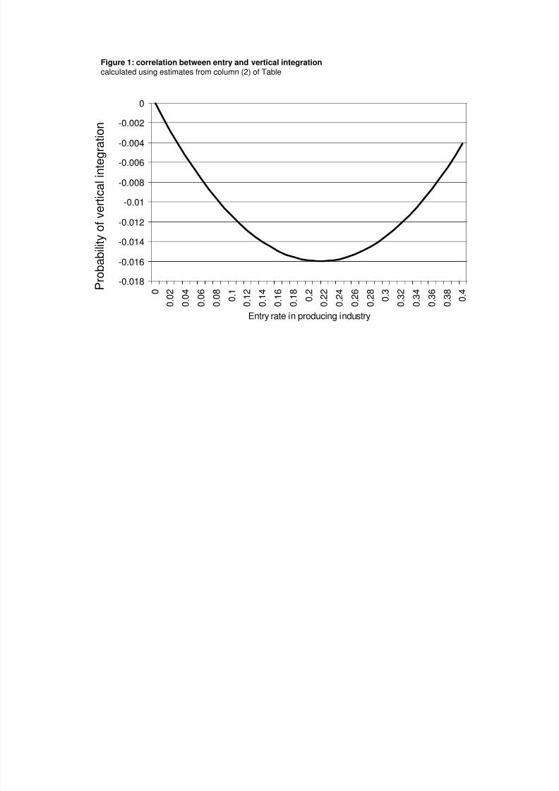
We show the correlation between our proxies of competition and the proportionof firms that are vertically integrated. We estimate the probability of being ver-tically integrated, so Proposition 3 implies this should be a U shaped. The firstcolumn of the Table shows the correlation between competition, as measuredby the entry rate, and the proportion of producing firms that are verticallyintegrated with a supplier. The probability of vertical integration is initiallydeclining in competition but then, at higher levels of competition, is increas-ing. In column (2) we include the entry rate in the supplying industry alongwith the age and size (measured by employment) of the producing firm and anindicator of whether the producing firm is foreign-owned. Figure 1 shows thepattern of this correlation, normalised to zero at zero entry. At lower levels of entry, as entry increases the probablity of vertical integration declines (in linewith both PRT and TCE approaches). This gradually diminishes, and above acertain level the correlation switches. As a robustness check in column (3) wealso include the share of inputs (used by producers) that are imported.

In column (4) we use an alternative entry rate, looking just at entry byforeign firms. We might be concerned that entry is a noisy measure of com-

petition. Foreignfi

rms are in general larger and represent a more substantialcompetitive threat.5 Figure 2 plots the relationship between entry and verticalintegration implied by these estimates. Here we see that the upward part of thecurve dominates - in line with the predictions of the PRT approach but not theTCE approach.

5 Concluding comments

In this paper we have provided some preliminary evidence to suggest that thereis a non-linear relationship between competition and the propensity of firms tovertically integrate. These results seem to be more consistent with the PropertyRight Theory (PRT) of vertical integration than with the Transaction CostEconomics (TCE) approach.



References

Aghion, Philippe, Bloom, Nick, Blundell, Richard, Griffith, Rachel, and Peter

Howitt (2005), ”Competition and Innovation: An Inverted-U RElationship”,

Quarterly Journal of Economics, Vol. 120, No. 2, pp. 701-728.

Acemoglu, Daron, Aghion, Philippe, Griffith, Rachel and Fabrizio Zilibotti(2004), “Vertical Integration and Technology: Theory and Evidence”, IFS Work-

ing Papers, W04/34.

Caves, Richard, and Ralph Bradburd (1988), ”The Empirical Determinants of

Vertical Integration”, Journal of Economic Behavior and Organizations , 9, 265-

279.

Feenstra, Robert (1998), “Integration of Trade and Disintegration of Produc-

tion”, Journal of Economic Perspective, 12, 31-50.

Grossman, Sandford and Oliver Hart (1986), ”The Costs and Benefits of Owner-

ship: A Theory of Vertical and Lateral Integration,” Journal of Political Econ-

omy, 94, 691-719.

Hart, Oliver and John Moore (1990), “Property Rights and the Nature of the

Firm”, Journal of Political Economy, 98, 1119-1158.

Joskow, Paul (1987), “Contract Duration and Relationship-Specific Investments:

Empirical Evidence from Coal Markets”, American Economic Review, 77, 168-

185.

Joskow, Paul (2003), “Vertical Integration”, forthcoming in the Handbook of

New Institutional Economics.

Klein, Benjamin (1998), “Vertical Integration As Organized Ownership: the

Fisher Body-General Motors Relationship Revisited” Journal of Law, Economics

and Organization, 4, 199-213.

Klein, Benjamin, Crawford, Robert, and Armen Alchian (1978), ”Vertical Inte-

gration, Appropriable Rents, and the Competitive Contracting Process,” Jour-

nal of Law and Economics, 21, 297-326



Implications, Free Press, New-York.

Williamson, Oliver (1985), The Economic Institutions of Capitalism, Free Press,

New-York..



Dep var: Proportion of firms

that are vertically integrated

(1) (2) (3) (4)

Producing entry rate -0.618

(0.104)

-0.149

(0.070)

-0.666

(0.101)

Producing entry rate2 0.989

(0.223)

0.347

(0.177)

1.023

(0.210)

Supplying entry rate 0.581

(0.084)

0.230

(0.029)

Supplying entry rate2 -1.462(0.199)

-0.106(0.033)

Producing foreign entry rate -0.606

(0.250)

Producing foreign entry rate2 11.507

(3.937)

Supplying foreign entry rate 1.524

(0.352)

Supplying foreign entry rate2 -50.712

(7.350)Age 0.006

(0.004)

0.003

(0.003)

0.008

(0.003)

Employment 0.012

(0.008)

0.01

(0.008)

0.012

(0.008)

Foreign-owned 0.081

(0.041)

0.036

(0.036)

0.090

(0.042)

Share of inputs imported -0.040

(0.016)

Year effects yes yes yes yes

Notes: Regressions include 15,990 observations at the industry-pair year level over the period 1980-1992.

The dependent variable is the proportion of firms in the industry pair that are vertically integrated. Numbers

in parentheses are robust standard errors that are clustered at the producing industry level. There are 181

producing industries.



-0.018

-0.016

-0.014

-0.012

-0.01

-0.008

-0.006

-0.004

-0.002

0

0

0 . 0

2

0 . 0

4

0 . 0

6

0 . 0

8

0 . 1

0 . 1

2

0 . 1

4

0 . 1

6

0 . 1

8

0 . 2

0 . 2

2

0 . 2

4

0 . 2

6

0 . 2

8

0 . 3

0 . 3

2

0 . 3

4

0 . 3

6

0 . 3

8

0 . 4

Entry rate in producing industry

P r o

b a b i l i t y o f v e

r t i c a l i n t e g r a t i o n

Figure 1: correlation between entry and vertical integration

calculated using estimates from column (2) of Table



-0.02

-0.01

0

0.01

0.02

0.03

0.04

0.05

0.06

0 0.01 0.02 0.03 0.04 0.05 0.06 0.07 0.08 0.09 0.1

Foreign entry rate in producing industry

P r o

b a b i l i t y o f v e

r t i c a l i n t e g r a t

i o n

Figure 2: correlation between foreign entry and vertical integration

calculated using estimates from column (4) of Table.

Vertical Integration and Competition

Documents

Transcript of Vertical Integration and Competition