Vermont Water Resources and Lake Studies Center Annual ...

Vermont Water Resources and Lake Studies Center Annual Technical Report

FY 2007

IntroductionThe Annual Report for the Vermont Water Resources and Lake Studies Center for FY2007 is attached.The grant awarded under the State Water Resources Research Institute Program is 06HQGR0123.

Research Program IntroductionOverview: The National Institute for Water Resources funds research projects through the Annual InstituteProgram administered by the U.S. Geological Survey Water Resources Institute Program. This annualgrants program is designed to promote research, training, information dissemination, and other activitiesmeeting the needs of the State of Vermont and the Nation. The program encourages submission ofresearch projects that address water resources problems important to Vermont and research projects thatstimulate the development of new and innovative areas.

The Vermont Water Resources and Lake Studies Center collaborated in a joint RFP with the RiverManagement Program in the Department of Environmental Conservation (Agency of Natural Resources).

While proposals on any topic relevant to the mission of the Water Center were considered, proposals thataddressed some aspect of the research needs expressed by the River Management Program were givenpriority for funding.

General objectives: The general objectives of this Joint RFP were as follows:

1. to advance scientific understanding that helps describe and quantify the contribution of sediment andnutrients derived from fluvial processes;

2. to establish the socio-economic justifications, costs, and benefits associated with or represented by rivercorridor protection; and

3. to contribute to Vermont’s river corridor management, restoration, and protection infrastructure.

Two areas of particular interest were noted, as follows:

Science Interests: Strengthening and validating Vermont’s draft fluvial geomorphic-based model fordescribing sediment regime departures from reference or equilibrium conditions, which may influence themagnitude of sediment and nutrient production, transport, and attenuation or storage on a watershed scale.Suggested research areas for the 2006 Joint RFP included:

A. Collect new and/or use existing data to test the draft fluvial-geomorphic-based model currently beingdeveloped by the River Management Program and generate innovative new map products.

B. Quantify how sediment and nutrient reductions may be achieved by managing river systems towardequilibrium conditions, and alleviating constraints to sediment load attenuation at a watershed scale.

C. Examine and quantify the P available to be mobilized by fluvial processes and represented in variousalluvial soil classifications.

D. Quantify sediment and P production in selected meso/macro scale examples. Relate to extant of fluvialgeomorphic evolution or adjustment processes and the driving forces and stressors for such adjustments.

E. Place fluvial adjustment processes and sediment/P production rates on a geologic time scale/continuumsuch that a comparison of rates of sediment/P delivery to the lake can be made (are there thresholds ofland use and channel /floodplain geometry change that should be considered).

Socio-Economic Interests: Socio-economic analyses that build upon the River Management AlternativesWhite Paper and other VT DEC River Management Program fact sheets and papers published by the RMPand available at http://www.anr.state.vt.us/dec/waterq/rivers.htm. Suggested research areas included:

A. Quantify the socio-economic costs and benefits of river corridor protection.

B. What economic factors have driven river and river corridor management historically (nineteenth andtwentieth centuries) as compared with current day economic drivers and how can differences behighlighted to change public perception/values? What trends or new factors are likely to be drivers in thefuture?

C. Identify/test/validate innovative voluntary landowner and municipal incentives that could be created inVermont to enhance participation in river corridor protection initiatives.

The RFP Process

A total of six proposals were received on or before the due date. One project funded in the 2005 RFP cyclewas assessed for progress toward proposed goals and was deemed to be worthy of a second year ofsupport. The remaining five proposals sought funding for new projects relevant to the 2006 RFP goals.

All six proposals were evaluated by the Vermont Water Center Advisory Board and two partners from theRiver Management Program (B. Cahoon and M. Kline). The Vermont Water Center Advisory Boardincludes members from the UVM faculty (B. Bowden and M. Watzin), a local environmental NGO (M.Winslow), a consulting firm (C. Heindel), and a staff member from the Vermont Agency of NaturalResources, but not associated with the River Management Program (D. Burnham). These reviewersevaluated each proposal according to specific criteria included in Appendix 1 and summarized as indicatedin Appendix 2. The Evaluation Committee then convened by teleconference on 19 December 2005 toshare evaluations and select proposals to forward for final submission to the USGS.

The following three projects were selected for funding:

1. Phosphorus Availability from the Soils Along Two Streams of the Lake Champlain Basin: Mapping,Characterization and Seasonal Mobility. Donald Ross, Joel Tilley, Eric Young, and Kristen Underwood.

2. An Adaptive Management System Using Hierarchical Artificial Neural Networks and Remote Sensingfor Fluvial Hazard Mitigation. Donna Rizzo and Leslie Morrissey

3. Riverbank Stability Evaluations: Comparing Quantitative Assessments to Qualitative RGA ScoresMandar Dewoolkar and Paul Bierman.

These projects were funded beginning 1 March 2006. Progress on the projects was reviewed in December2006 by the Water Center Advisory Board, including Mike Kline and Barry Cahoon and all three projectswere recommended for continued funding through the 2007-2008 project year (ending 28 February 2008).Final reports for each of these projects are provided.

Evaluating Quantitative Models of Riverbank Stability

Basic Information

Title: Evaluating Quantitative Models of Riverbank Stability

Project Number: 2006VT25B

Start Date: 3/1/2006

End Date: 2/29/2008

Funding Source: 104B

Congressional District: First

Research Category: Engineering

Focus Category: Sediments, Models, Geomorphological Processes

Descriptors:

Principal Investigators: Mandar M. Dewoolkar, Paul Bierman

Publication1. Borg, Jaron. 2007. Northeast Geotechnical Symposium at University of Massachusetts at Amherst,

and Lake Research Conference - "Lake Champlain: Our Lake, Our Future." Burlington, VT.

Project 1

Evaluating Quantitative Models of Riverbank Stability

Mandar Dewoolkar and Jaron Borg, School of Engineering University of Vermont

and Paul Bierman, Department of Geology

University of Vermont

Background

This research examined what makes some banks stable and other banks fail over time with changing river and groundwater conditions. The goal was to develop a reliable quantitative model of streambank slope stability and erosion. To develop such a model, quantitative and semi-quantitative approaches were adopted. The quantitative approach utilized an in-depth geotechnical analysis incorporating measured soil strength parameters, water levels, bank geometries and failure processes. The semi-quantitative approach is similar; however, the soil strength parameters were empirically correlated to soil index properties. Streams, Sites and Instrumentation

During the summers of 2006 and 2007 a reach from two streams (Winooski River and Lewis Creek) in the Lake Champlain Basin were selected for the study. Seven to eight cross-sections were selected on each reach of streambank, some on the verge of failure and some marginally stable, were surveyed and subsurface investigations were performed to determine the soil characteristics. On both reaches, one cross section was instrumented with various monitoring equipment. Figure 1.1a shows a photograph of the site on Winooski near Ethan Allen Homestead (also seen as larger blue circle in Figure 1.1b) instrumented in summer 2006. The other seven sampling locations are shown as smaller purple circles in Figure 1.1b. All locations were chosen along the outer bank of a meander bend, often called a cutbank, in the river because this is where we expected the most erosion. Of these eight locations, four appeared to be unstable and four appeared to be marginally stable. Figure 1.1b shows how the banks of the river have changed between 1962 and 2004 from aerial photographs. In summer 2007, we selected sites along Lewis Creek in North Ferrisburg and similarly instrumented as the reach on the Winooski.

(a) Bank of Winooski River

(b) Site locations

Figure 1.1. Selected site locations along Winooski River and analysis of aerial photos

A typical instrumentation plan is depicted in Figure 1.2. It includes pore water pressure transducers to track changes in groundwater levels. In addition, several tilt switches were embedded in the bank wirelessly connected to a computer in the Winooski Valley Park District Office, which is about 600

feet from the instrumented site. Unfortunately, the transmitters for these switches were vandalized and valuable data were lost. Therefore, at the end of summer 2007 new tilt switches were installed in the banks of both instrumented sites with data loggers that were imbedded in the ground in weatherproof lock boxes making them not easily accessible(see Figures 1.2 and 1.3). These tilt switches register a signal on the data logger if they were to go out of alignment by more than 10 degrees. The data logger for the site on the Winooski has been retrieved and has registered a single tilt activation point, which corresponded to the increase in groundwater levels (Figure 1.4). The tilt switch data from Lewis creek could not be retrieved for the 2007-2008 season as the weather proof box was removed without our knowledge by a trespasser. In addition to the pore water pressure transducers and tilt switches, rain gauges were also installed at each instrumented site. The data from the rain gages and pore pressure transducers have been reliable.

At each testing site, GPS coordinates were taken as well as several photographs. We also developed procedures for obtaining detailed surveys of bank cross-sections, which are being used to track changes in the stream bank geometry for slope stability analyses. The water level monitoring equipment has been proven to function properly and a 180 day data set has been recorded in conjunction with the tilt switch activation on 1/10/08 at 9:00am.

Site Characterization Several 3’’ boreholes were hand augered at

each of the sites to observe the soil profiles and obtain low disturbance Shelby tube samples. In-situ borehole shear tests (BST) were performed at these sites to determine soils’ shear strength parameters - cohesion and internal friction angle. The shear strength (in the form of Mohr-Coulomb envelope) of a silty sand layer at Winooski sites remain fairly consistent across several sites investigated. As an example, Figure 1.5 shows failure shear stresses as a function of applied normal stresses from borehole

shear tests. As expected, the failure envelope was found to be linear using the BST. Laboratory direct shear tests were also performed on soil samples recovered from the sites to verify shear strength determined from borehole shear tests. Typically, the agreement was very good, with the direct shear tests generally being 1-3˚ higher than those observed in the field. Other measurements, such as soil suction, in-situ moisture and density were also obtained at the sites. Methods for evaluating effects of grass roots on

Figure 1.2. Various Sensors installed at the instrumented site

Figure 1.3. Photo of new tilt switch system prior to implanting in the field

Water Levels Observed at Winooski Site

-10

-8

-6

-4

-2

0

2

4

6

5/17/0

7

5/31/0

7

6/14/07

6/28/0

7

7/12/0

7

7/26/0

78/9

/07

8/23/0

79/6

/07

9/20/0

7

10/4/

07

10/18

/07

11/1/

07

11/15

/07

11/29

/07

12/13

/07

12/27

/07

1/10/0

8

Data collection number

Unc

ompe

nsat

ed W

ater

Col

umn

(ft)

Tilt

Switc

h M

easu

red

Volta

ge

Well 1Well 2Well 3tilt_switch

Figure 1.4. Ground water levels at the Winooski site from 05/07 to 01/08. Tilt switch activation indicated with arrow

soil’s strength were also investigated in summer 2007 offering insights into changes to the strength of soils due to root tensile strength (see Figure 1.6).

Figure 1.5. Shear stress versus normal stress data from BST tests conducted in silty sand at the selected sites

Figure 1.6. Plot obtained from tensile testing of Solidago rugosa roots present in most cross sections at both reach selections

Slope Stability Analysis

The stability of several slopes was evaluated in two slope stability models using the cross sectional surveys and measured soil properties and some estimated parameters. The “Bank Stability and Toe Erosion” model (Simon, et al., 2003) proved simple to use, but only allowed linear potential failure surfaces and horizontal water levels in the slope and the stream. An example of this model for the Winooski site is shown in Figure 1.7. Our field observations however indicated multiple nonlinear failure surfaces along both reaches of rivers. Our preliminary analysis indicated that this model would have to be modified or redesigned to incorporate multiple nonlinear failure geometries.

The second slope stability model used was the computer program SLOPE/W, which is versatile, but complicated and expensive. Figure 1.8 shows some of our SLOPE/W analysis and illustrates the effects of stream and groundwater levels on bank stability. The instrumented Winooski slope in these figures was analyzed with measured soil properties, estimated apparent cohesion, and measured water level conditions for three instances in time. Figures 1.8a and b, show the slope with water levels at the same elevation in the stream and the bank. Computed factors of safety against rotational slope failure are also shown. The value shown, just above 1.0 indicates that the bank at this point in time is marginally stable (1.0 indicates “verge of failure”). As was expected, higher water levels resulted in a higher factor of safety because mass of the water in the stream provided stabilizing force. Figure 1.8c shows the same slope as before, but now the water level in the stream has dropped rapidly by 3 feet. The groundwater in the bank did not drain because the soil’s permeability did not allow the water in the bank to drain as quickly as the water changed in the river. In this “rapid drawdown” type situation, the bank becomes unstable, i.e. the factor of safety drops below 1.0 indicating a slope failure.

Figure 1.7. Bank Stability and Toe Erosion Model output for the Winooski site

(a) (b) (c)

Figure 1.8. Slope stability analysis of the instrumented Winooski slope for varying water levels

These same situations were also modeled using soil densities and shear strengths estimated based

on their index properties using widely available empirical correlations suggested by Naval Facilities Engineering Command (NAVFAC, 1982), as a “semi-quantitative” analysis. Although this model used lower values for shear strength of the soils, the factors of safety were increased in all situations due to lower bulk unit weight of the soils suggested by NAVFAC (see Figure 1.9). However, the trend in the factors of safety numbers with changing water levels was similar in both sets of analyses (quantitative and semi-quantitative).

(a) Fs= 1.28 (b) Fs= 1.23 (c) Fs=1.09

Figure 1.9. Slope stability of instrumented site using averaged NAVFAC index properties

New Model Development

In order to analyze the study banks over a period of time incorporating changing water levels, one would have to run the current models manually numerous times. An automated procedure would be highly desired for this type of temporal analysis. To automate this procedure, efforts were directed in creating a slope stability and erosion modeling program using the MATLAB programming system.

This new model is expected to be capable of evaluating the stability of a particular slope by initially discretizing the soil above a potential failure surface into slices and then evaluating the driving and resisting forces/moments on each of the slices. The program receives geometric inputs of the water table, slope geometry, and trial failure surface in x and y coordinates. It also requires the inputs of the internal friction angle, cohesion, and unit weight of the soils. The program then outputs the factor of safety for the slope using the particular failure surface being evaluated. Although this program produces results similar to those found by using the SLOPE/W program debugging is still necessary to increase its reliability.

The model also has a routine under development that attempts to incorporate the geomorphic changes due to erosion of the streambanks. This is done by discretizing the bank geometry into a series of points designated by x and y coordinates. The coordinates of the points are then modified using the product of the erosion rate and the timestep length.

Training

So far, one MS, one PhD and six undergraduate students had direct involvement in this project. Out of these, two graduate and two undergraduate students were partially supported through this grant. Support for the remaining four undergraduate students was obtained through other sources (URECA!, Richard Barrett Foundation, NSF-funded Math-Bio program, and Workstudy). In addition to above mentioned students, a total of about 35 engineering students have benefited indirectly from this research over two years. These students used the borehole shear test apparatus, field augering and sampling equipment acquired through the grant for their service-learning projects in Prof. Dewoolkar’s Geotechnical Design course. The projects included evaluation of foundations, retaining structures and slopes at historic structures in Vermont.

Conclusions

The following conclusions are drawn based on the results obtained thus far:

1) The instrumentation (piezometers, rain gauges, and tilt switches) provided reasonably reliable information at the instrumented streambanks (groundwater levels, rain, and slope failure) as a function of time.

2) The borehole shear tests provided reliable measurements of soil shear strengths. The shear strength parameters obtained from conducting laboratory direct shear tests were generally close to the shear strength parameters determined in-situ using the borehole shear tests.

3) The Bank Stability and Toe Erosion model appears to be not suitable for modeling the Winooski and Lewis Creek streambank failures, which are rotational. The model allows only straight line failure surfaces.

4) The SLOPE/W model is suitable for modeling slope stability at a particular time instance; however, it would be a cumbersome process to use this model to quantify slope stability factor of safety as a function of time.

5) The semi-quantitative slope stability analysis showed similar trends to the quantitative analysis.

Results Yet to be Reported

Updated surveys will need to be taken to show how the stream banks have changed between 2007 and 2008. Conducting these surveys is not possible earlier in the year. The swelled rivers and cold waters of at the research locations pose serious danger to those surveying the banks. Additional measurements of soil strength will be made at several sites where more data are needed.

Efforts will be directed in the determination of the erosion rates of the soils in our research areas. Currently there are two different approaches that are being considered to do this. Jaron Borg will be attending a course on streambank erosion at the end of June 2008 where determination and prediction of the erodibility of soils will be discussed. It is hoped that this will bring expertise to make reliable

estimates of the soil’s erosion properties. The second method is to determine an apparent erodibility rate by back-calculating the erodibility rate by using a set of cross sectional surveys with close temporal resolution.

We anticipate that the remainder of the project period will be spent on refining and calibrating the new combined stability and erosion model that is being developed. It is expected that the model will be able to use the observed water levels in the field as a function of time and also predict the changes in slope geometry from erosion, and the stability of a streambank can then be quantified over time and changing water conditions.

References

NAVFAC (1982), U.S. Naval Facilities Engineering Command Manual Foundations and Earth Structures, NAVFAC Design Manual 7.2, Arlington, VA.

Simon, A., Langendoen, E.J., Collison, A., Layzell, A. (2003), Incorporating bank-toe erosion by hydraulic shear into a bank-stability model: Missouri River, Eastern Montana”, Proceedings, EWRI-ASCE, World Water & Environmental Resources Congress,11p.

An Adaptive Management System using Hierarchical ArtificialNeural Networks and Remote Sensing for Fluvial HazardMitigation

Basic Information

Title: An Adaptive Management System using Hierarchical Artificial Neural Networksand Remote Sensing for Fluvial Hazard Mitigation



End Date: 2/29/2008



Research Category: Water Quality

Focus Category: Geomorphological Processes, Hydrology, Models

Descriptors:

Principal Investigators: Donna Rizzo, Leslie Morrissey

Publication

Project 2 An Adaptive Management System using Hierarchical Artificial Neural Networks and

Remote Sensing for Fluvial Hazard Mitigation

Donna Rizzo, School of Engineering University of Vermont

and Leslie A. Morrissey, Rubenstein School of Environment and Natural Resources


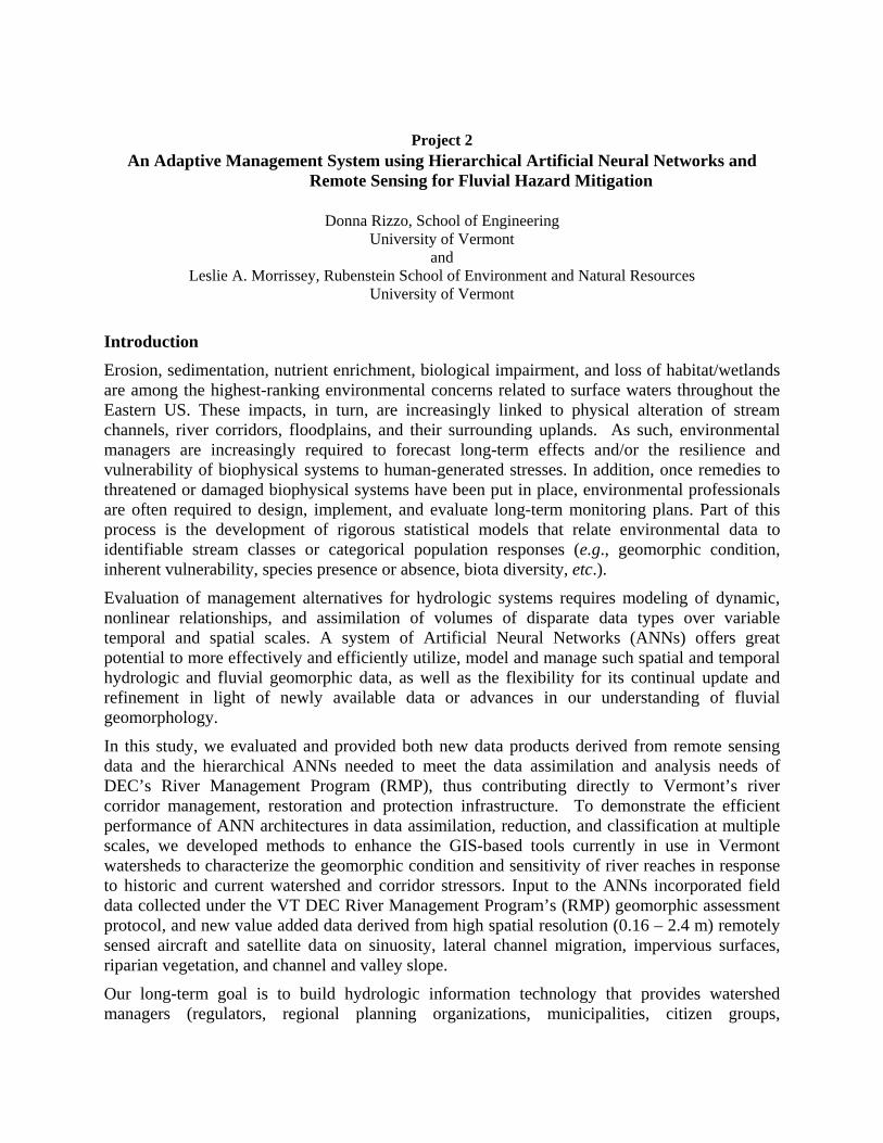
Introduction Erosion, sedimentation, nutrient enrichment, biological impairment, and loss of habitat/wetlands are among the highest-ranking environmental concerns related to surface waters throughout the Eastern US. These impacts, in turn, are increasingly linked to physical alteration of stream channels, river corridors, floodplains, and their surrounding uplands. As such, environmental managers are increasingly required to forecast long-term effects and/or the resilience and vulnerability of biophysical systems to human-generated stresses. In addition, once remedies to threatened or damaged biophysical systems have been put in place, environmental professionals are often required to design, implement, and evaluate long-term monitoring plans. Part of this process is the development of rigorous statistical models that relate environmental data to identifiable stream classes or categorical population responses (e.g., geomorphic condition, inherent vulnerability, species presence or absence, biota diversity, etc.).

Evaluation of management alternatives for hydrologic systems requires modeling of dynamic, nonlinear relationships, and assimilation of volumes of disparate data types over variable temporal and spatial scales. A system of Artificial Neural Networks (ANNs) offers great potential to more effectively and efficiently utilize, model and manage such spatial and temporal hydrologic and fluvial geomorphic data, as well as the flexibility for its continual update and refinement in light of newly available data or advances in our understanding of fluvial geomorphology.

In this study, we evaluated and provided both new data products derived from remote sensing data and the hierarchical ANNs needed to meet the data assimilation and analysis needs of DEC’s River Management Program (RMP), thus contributing directly to Vermont’s river corridor management, restoration and protection infrastructure. To demonstrate the efficient performance of ANN architectures in data assimilation, reduction, and classification at multiple scales, we developed methods to enhance the GIS-based tools currently in use in Vermont watersheds to characterize the geomorphic condition and sensitivity of river reaches in response to historic and current watershed and corridor stressors. Input to the ANNs incorporated field data collected under the VT DEC River Management Program’s (RMP) geomorphic assessment protocol, and new value added data derived from high spatial resolution (0.16 – 2.4 m) remotely sensed aircraft and satellite data on sinuosity, lateral channel migration, impervious surfaces, riparian vegetation, and channel and valley slope.

Our long-term goal is to build hydrologic information technology that provides watershed managers (regulators, regional planning organizations, municipalities, citizen groups,

landowners, and other stakeholders) with an easy-to-use, graphical infrastructure for adaptive and effective decision-making at multiple spatial and temporal scales.

Background Recent advances in the computational and statistical sciences have led to the development of sophisticated methods for parametric and nonparametric analysis of data with categorical responses. Our research applies these new statistical analyses on recently collected watershed data and repackages these techniques in the form of a hierarchical suite of ANNs.

At the state level, the VTANR has been developing and testing protocols for conducting remote sensing and field-based fluvial geomorphic and physical habitat assessments since 1999. Our modeling system is directly applicable to the fluvial hazard mitigation mission of the River Management Program (ANR/DEC), but differs sharply from conventional hydrologic models currently in use by the volume, variety, and types of spatial and temporal data assimilated. Moreover, the architecture of a hierarchical ANN system is sufficiently flexible to allow for its continual update and refinement in light of advances in our understanding of fluvial geomorphology. Our research goal was to evaluate not only a new and innovative data assimilation and analysis methodology, but also data products derived from remote sensing imagery that offer the potential to substantially improve hydrological modeling in Vermont. In addition, our method compliments the existing RMP state program, taking advantage of existing data, protocols, and personnel – a modeling approach that could be adopted statewide.

RESULTS (June 2006-June 2008)

We have developed and tested a hierarchical ANN system to more effectively integrate, model, and manage spatial and temporal hydrologic and fluvial geomorphic data, and also incorporating data products derived from very high resolution remote sensing imagery.

Selection of Study Area: The research focused on two stormwater impaired watersheds in Chittenden County, VT to take advantage of both the existing VT ANR River Management Program (RMP) field measurement efforts and available high resolution remotely sensed data. Allen Brook (16 reaches) and Indian Brook (25 reaches) were selected for analysis in collaboration with DEC RMP.

Recruitment of Graduate Students: Two graduate students were recruited to support the two major research objectives of this project. Lance Besaw (Ph.D. student) joined the civil engineering program to conduct statistical analyses and ANN modeling efforts under the direction of Donna Rizzo. Keith Pelletier (M.S. student) joined the RSENR graduate program to perform remote sensing analyses under the direction of Leslie Morrissey.

RESEARCH OBJECTIVES: The specific objectives were to:

Objective 1: Refine, test, and evaluate a set of simple classification ANNs for assessing the geomorphic condition and inherent vulnerability of stream reaches.

Objective 2: Derive and evaluate improved hydrologic information using remote sensing observations as input parameters in the ANN hierarchy. These new data include: a) stream

sinuosity, b) lateral channel migration, c) channel slope and valley slope, d) steep banks, e) riparian vegetation, and f) total and effective impervious areas.

OBJECTIVE 1 ARTIFICIAL NEURAL NETWORS

Task 1.1—Refine Geomorphic and Inherent Vulnerability ANNs incorporating Remote Sensing data.

Artificial Neural Networks (ANNs) are dynamic computational systems built with interconnected processing units (nodes) that interact with each other in a parallel manner. The architecture is made up of input, hidden and output nodes (grey circles in subsequent figures). ANNs are viewed as universal approximators and are useful for mapping some input space to some output space (e.g. see Figure 2.1(a) with inputs consisting of entrenchment ratio, width/depth ratio, etc. and outputs consisting of the desired stream type classification). The training procedure may be described, in general terms, as mapping the non-linear relationships between collected input-output data pairs. Many training algorithms exist to iteratively adjust the internal parameters (weights) to better simulate (or learn) the desired mapping. A detailed description of the counterpropagation algorithm used for this work is included in Appendix A. This particular algorithm has the ability to extract physical meaning from the internal parameters based on the ANN inputs, for more details please refer to (Rizzo and Dougherty 1994a; and Besaw and Rizzo 2007). During Year 1, research and development was initially performed on a proof-of-concept prototype of the proposed counterpropagation ANN tool (Task 1.1). A hierarchal system of ANNs has been developed to predict stream sensitivity using VTANR Phase II rapid stream assessment data (hereafter referred to as the Phase II dataset). The first of the two ANNs in series, utilizes inputs of channel geometry and bed form to predict a modified Rosgen channel classification (stream type). This ANN was tested using Phase II data collected from five selected streams. Of the 89 reaches and segments, 72 (81%) were classified by the ANN correctly when compared to stream type classification reported in the Phase II assessment.

(b) Stream sensitivity ANN (a) Rosgen ANN

Single/multiple channel(s) Entrenchment ratio Stream type

Figure 2.1. Graphical representation of (a) the modified Rosgen ANN used to determine stream type and (b) ANN for determining VTANR stream sensitivity using inputs of stream type and condition.

The second of the two ANNs was used to predict stream sensitivity (as described by VTANR) using inputs of stream type (output from first ANN) and stream condition (Phase II RGA score). The same 89 reaches were used to evaluate the performance of this ANN. Of the 89 reaches and

Width/depth ratio VTANR Stream

sensitivity Sinuosity Slope

… Stream

condition

… Channel material

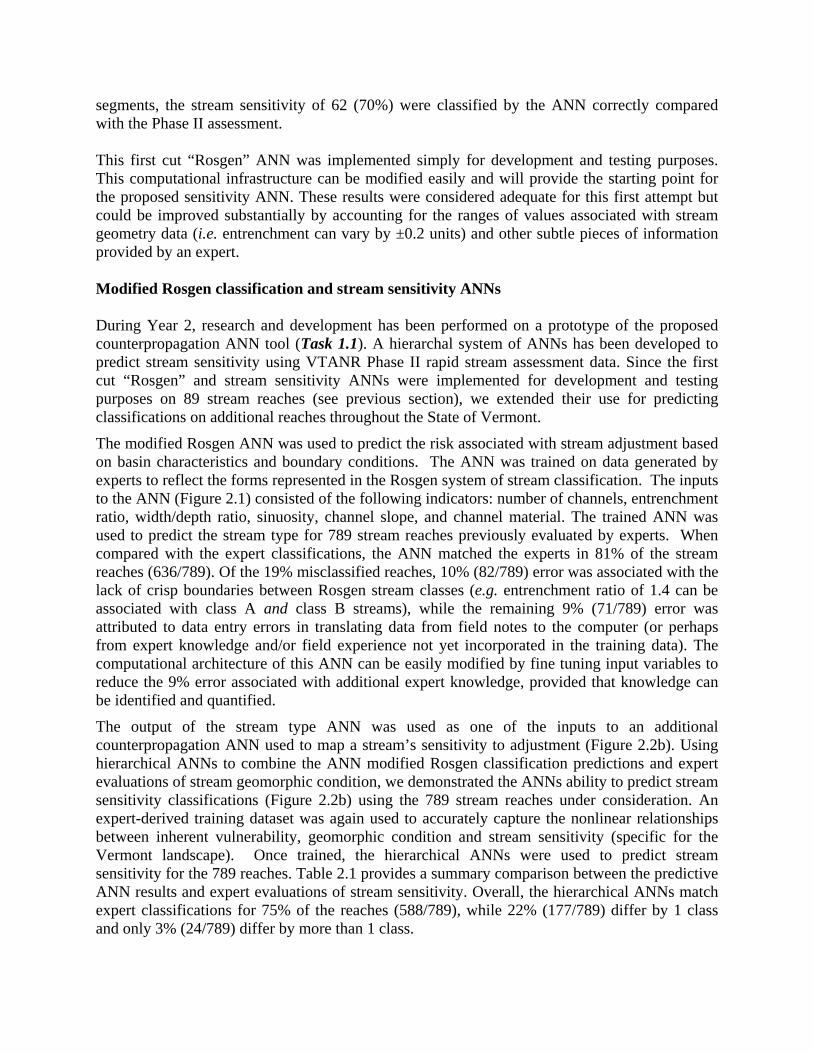
segments, the stream sensitivity of 62 (70%) were classified by the ANN correctly compared with the Phase II assessment. This first cut “Rosgen” ANN was implemented simply for development and testing purposes. This computational infrastructure can be modified easily and will provide the starting point for the proposed sensitivity ANN. These results were considered adequate for this first attempt but could be improved substantially by accounting for the ranges of values associated with stream geometry data (i.e. entrenchment can vary by ±0.2 units) and other subtle pieces of information provided by an expert. Modified Rosgen classification and stream sensitivity ANNs During Year 2, research and development has been performed on a prototype of the proposed counterpropagation ANN tool (Task 1.1). A hierarchal system of ANNs has been developed to predict stream sensitivity using VTANR Phase II rapid stream assessment data. Since the first cut “Rosgen” and stream sensitivity ANNs were implemented for development and testing purposes on 89 stream reaches (see previous section), we extended their use for predicting classifications on additional reaches throughout the State of Vermont.

The modified Rosgen ANN was used to predict the risk associated with stream adjustment based on basin characteristics and boundary conditions. The ANN was trained on data generated by experts to reflect the forms represented in the Rosgen system of stream classification. The inputs to the ANN (Figure 2.1) consisted of the following indicators: number of channels, entrenchment ratio, width/depth ratio, sinuosity, channel slope, and channel material. The trained ANN was used to predict the stream type for 789 stream reaches previously evaluated by experts. When compared with the expert classifications, the ANN matched the experts in 81% of the stream reaches (636/789). Of the 19% misclassified reaches, 10% (82/789) error was associated with the lack of crisp boundaries between Rosgen stream classes (e.g. entrenchment ratio of 1.4 can be associated with class A and class B streams), while the remaining 9% (71/789) error was attributed to data entry errors in translating data from field notes to the computer (or perhaps from expert knowledge and/or field experience not yet incorporated in the training data). The computational architecture of this ANN can be easily modified by fine tuning input variables to reduce the 9% error associated with additional expert knowledge, provided that knowledge can be identified and quantified.

The output of the stream type ANN was used as one of the inputs to an additional counterpropagation ANN used to map a stream’s sensitivity to adjustment (Figure 2.2b). Using hierarchical ANNs to combine the ANN modified Rosgen classification predictions and expert evaluations of stream geomorphic condition, we demonstrated the ANNs ability to predict stream sensitivity classifications (Figure 2.2b) using the 789 stream reaches under consideration. An expert-derived training dataset was again used to accurately capture the nonlinear relationships between inherent vulnerability, geomorphic condition and stream sensitivity (specific for the Vermont landscape). Once trained, the hierarchical ANNs were used to predict stream sensitivity for the 789 reaches. Table 2.1 provides a summary comparison between the predictive ANN results and expert evaluations of stream sensitivity. Overall, the hierarchical ANNs match expert classifications for 75% of the reaches (588/789), while 22% (177/789) differ by 1 class and only 3% (24/789) differ by more than 1 class.

From a management perspective such a hierarchy of ANNs could prove useful for QA/QC. For example, when the ANN predictions differ from the expert evaluations, this may either: 1) highlight errors due to data entry and/or 2) provide an opportunity to extract additional information and reasoning from the experts about their decision-making process, as the expert may be observing stream conditions not currently included in the existing training dataset. Table 2.1. Hierarchical ANN and expert predictions of stream sensitivity.

ANN Predictions Very Low Low Medium High Very High Extreme

Very Low 6 2 0 0 1 0 Low 0 0 1 3 0 1

Moderate 0 0 58 27 4 0 High 0 0 20 231 37 1

Very High 0 0 1 44 284 2

Exp

ert

Pred

ictio

ns

Extreme 0 0 0 13 44 9

Planform change ANN Next, a new counterpropagation ANN was trained and tested for predicting planform change on 652 stream reaches using field data provided in the VTANR Phase II protocols. From the Phase II handbook, a total of 18 variables were selected as potential predictors of planform change. These 18 predictor variables and their coded format are shown in Table 2.1. Traditional statistical techniques are not suitable for the task of predicting planform change because more than half of the predictor variables are not continuous (e.g. bank slope, bank texture, etc. are categorical). The categorical predictors have been coded as integers in this work, and many of the predictors have been combined to summarize the reach characteristics on both the left and right side of the channel (or upper and lower sections of banks, as applicable).

Table 2.2. Predictor variables and data coding considered for the planform change ANN.

Number Class Code Value Combination Channel Slope Continuous >=0 No

Confinement ratio Continuous >=1 No Encroachment/(W/D) Continuous >=0 No

Confinement type Integer 1=narrowly , 2=semi-, 3=narrow, 4=broad,

5=very broad No

Entrenchment ratio Continuous >=1 no

Bank slope Integer 1=undercut, 2=steep, 3=moderate, 4=shallow left and right summed

Bank texture Integer

1=sand, 2=silt/clay and mix, 3=gravel,

4=boulder/cobble, 5=bedrock

upper and lower summed

Erosion/(W/D) Continuous >=0 no

Bank revetments Integer 1=none, 2=other, 3=hard bank and rip-rap left and right summed

Revetment length/(W/D) Continuous >=0 left and right summed

Dom. bank vegetation Integer

1=none and bare, 2= lawn and pasture, 3=invasives and

herbaceous, 4=shrubs/saplings, 5=coniferous and

deciduous

left and right summed

Sub. bank vegetation Integer (same as dominant bank vegetation) left and right summed

Mass failures Integer 1=multiple, 2=one, 3=none no

Total number of bars Integer 0, 1, 2… no Flood chutes Integer 0, 1, 2… no

Channel avulsions Integer 0, 1, 2… no Braiding Integer 0, 1, 2… no

Human alterations Integer 0=no, 1=yes straightening and/or dredging

Task 1.2 – Identify “critical” geomorphic variables: During Year 1, a preliminary sensitivity analysis was performed to identify “critical” geomorphic variables needed for the proposed stream sensitivity ANN (Module A). First, we examined which of the available VTANR Phase I and Phase II geomorphic assessment data were most influential (statistically) in predicting stream sensitivity and geomorphic condition (using multivariate statistics). Stepwise discriminant and canonical analysis are multivariate statistical methods commonly used for classification prediction. These techniques are well suited to identify which variables contribute to discriminating classifications.

Stream sensitivity provided in the Phase II database was classified into 6 categories using the geomorphic assessment (integer values ranging from very low = 1, low = 2, moderate = 3, high = 4, very high = 5 and extreme = 6). Table 2.3 displays the impact of each of the geomorphic variables ranked in decreasing order of importance when used as a predictor of classified stream sensitivity. This rank ordered list was produced using discriminant analysis (SAS Version 8.0). Table 2.3. Geomorphic variables rank ordered in importance for predicting stream sensitivity.

Rank Variable Number Class Code Value

1 Substrate D50 Integer 1=sand, 2=gravel, 3=cobble, 4=boulder and 5=bedrock

2 Watershed size Continuous >=0 3 Width/depth ratio Continuous >=1 4 Number of stormwater inputs Integer 0, 1, 2, 3, etc. 5 Change in valley slope Continuous + to - infinity 6 Change in channel slope Continuous + to - infinity 7 Upstream sinuosity Continuous >=1 8 Entrenchment Continuous >=1

9 Cumulative urban watershed size (%) Continuous >=0 (summation of upstream conditions)

10 Urban watershed size (%) Continuous >=0 11 Number of grade controls Integer 0, 1, 2, 3, etc. 12 Confinement ratio Continuous >=1 13 Number of upstream stormwater inputs Integer 0, 1, 2, 3, etc.

14 Least forwarded buffer width Integer 1=<5ft, 2=5-25ft, 3=26-50ft, 4=51-100ft, 5=>100ft

15 Channel slope Continuous >= 0 16 Valley slope Continuous >= 0 17 Sinuosity Continuous >=1 18 Straightening Binary 1-yes, 0-no

The rankings were a result of a simple stepwise discriminant analysis. Note that change in channel and valley slope over time and upstream sinuosity (ranked 5, 6 and 7 respectively) were among the four most important variables specifically related to stream morphology. In contrast, measures of channel and valley slope at any point in time, and sinuosity for a given reach were among the least important variables. This is due to the relative importance of variables 5 through 7 (∆ valley slope, ∆ in channel slope and upstream sinuosity). The top 11 (statistically significant) variables were included in the canonical plot of Figure 2.2. The 11 indicator variables shown on this canonical plot (represented by the lines/vectors) represent the direction and magnitude of the influence that each of the variables has in discriminating between the classes. This plot represents the separability of the 6 stream sensitivity classifications using the top 11 predictor variables. The + and radius of each of the circles represent the centroid and the 95% confidence interval for each of the 5 classifications respectively. Class 2 (low sensitivity) was not represented by any of the 58 stream reaches in this study area.

-4

-3

-2

-1

0

1

2

3C

anon

ical

2

1

3

45

6

Width/Depth Ratio (Ph2)Entrenchment (Ph2)

Substrate D50Number of Grade Controls

Stormeater Inputs (Ph2)

Watershed Size (Ph1)

Valley Slope Change from Upstream

Upstream Sinuosity

Urban Watershed % (Ph1)

Total Urban Watershed (%)

0 1 2 3 4 5 6 7 8 9Canonical1

Channel Slope Change from Upstream (Ph1)

Figure 2.2. Canonical plot of indicator variables for stream sensitivity ( + represents the mean of that respective class and the “vector” represents direction and magnitude of influence of each associated variable in discriminating between the classes).

Table 2.4 summarizes the stream reach sensitivity classification results using the discriminant equations. For the 58 stream reaches that make up the study area, the stepwise discriminant equations were able to correctly classify the stream sensitivity for 41 of the 58 reaches. This results in 17 of the reaches being misclassified (with 12 reaches that should be classified as type 5 (very high) classified as type 4 (high); and another 9 that should have classified as type 6 (extreme) classified as type 5 (very high).

Table 2.4. Results of predicting stream sensitivity prediction using discriminant analysis.

Classified by Discriminant Analysis Class 1 2* 3 4 5 6

1 1 0 0 0 0 0 2* 0 0 0 0 0 0 3 0 0 3 0 0 0 4 0 0 0 12 8 0 5 1 0 0 9 24 0

Classified in Phase II Assessment

6 0 0 0 0 0 1 *Note: There were no classifications of 2 (low sensitivity) in the dataset.

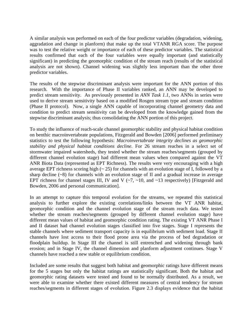
A similar analysis was performed on each of the four predictor variables (degradation, widening, aggradation and change in planform) that make up the total VTANR RGA score. The purpose was to test the relative weight or importance of each of these predictor variables. The statistical results confirmed that each of the four variables were equally important (and statistically significant) in predicting the geomorphic condition of the stream reach (results of the statistical analysis are not shown). Channel widening was slightly less important than the other three predictor variables. The results of the stepwise discriminant analysis were important for the ANN portion of this research. With the importance of Phase II variables ranked, an ANN may be developed to predict stream sensitivity. As previously presented in ANN Task 1.1, two ANNs in series were used to derive stream sensitivity based on a modified Rosgen stream type and stream condition (Phase II protocol). Now, a single ANN capable of incorporating channel geometry data and condition to predict stream sensitivity can be developed from the knowledge gained from the stepwise discriminant analysis; thus consolidating the ANN portion of this project. To study the influence of reach-scale channel geomorphic stability and physical habitat condition on benthic macroinvertabrate populations, Fitzgerald and Bowden [2006] performed preliminary statistics to test the following hypothesis: Macroinvertabrate integrity declines as geomorphic stability and physical habitat conditions decline. For 26 stream reaches in a select set of stormwater impaired watersheds, they tested whether the stream reaches/segments (grouped by different channel evolution stage) had different mean values when compared against the VT ANR Biota Data (represented as EPT Richness). The results were very encouraging with a high average EPT richness scoring high (~ 25) for channels with an evolution stage of I, followed by a sharp decline (~8) for channels with an evolution stage of II and a gradual increase in average EPT richness for channel stages III, IV and V (~7, ~10, and ~13 respectively) [Fitzgerald and Bowden, 2006 and personal communication]. In an attempt to capture this temporal evolution for the streams, we repeated this statistical analysis to further explore the existing correlations/links between the VT ANR habitat, geomorphic condition and the channel evolution stage of the stream reach data. We tested whether the stream reaches/segments (grouped by different channel evolution stage) have different mean values of habitat and geomorphic condition rating. The existing VT ANR Phase I and II dataset had channel evolution stages classified into five stages. Stage I represents the stable channels where sediment transport capacity is in equilibrium with sediment load. Stage II channels have lost access to their flood prone area via the process of bed degradation or floodplain buildup. In Stage III the channel is still entrenched and widening through bank erosion; and in Stage IV, the channel dimension and planform adjustment continues. Stage V channels have reached a new stable or equilibrium condition. Included are some results that suggest both habitat and geomorphic ratings have different means for the 5 stages but only the habitat ratings are statistically significant. Both the habitat and geomorphic rating datasets were tested and found to be normally distributed. As a result, we were able to examine whether there existed different measures of central tendency for stream reaches/segments in different stages of evolution. Figure 2.3 displays evidence that the habitat

rating scores are not statistically similar for streams at different stages of evolution. This means that the streams in different evolutionary stages have statistically different means. Streams in stage I have statistically higher habitat ratings than streams in stages II, III and IV. We only had one stream that classified as stage V within the study area data set.

Geo

mor

phic

Rat

ing

(Ph2

)

-0.10

0.10.20.30.40.50.60.70.80.9

I II III IV V

Channel Evolution Stage

Hab

itat R

atin

g (P

h2)

0.4

0.5

0.6

0.7

0.8

0.9

I II III IV V


Figure 2.3. Stem and box plots comparing (a) geomorphic and (b) habitat rating scores grouped by channel evolution stage for Phase II data from selected streams with LIDAR data.

Similar results were observed in the mean geomorphic condition scores, when grouped by evolutionary stage (Figure 2.4a). Stage I streams have higher geomorphic condition scores than the other stages. We also saw a slight increase in geomorphic condition in stream evolution stage IV compared to stage II and III. However these differences were not statistically separable for this dataset. Based on these statistical findings, ANN analysis and modeling can be attempted to capture the temporal component in the evolution of channel stage adjustment.

Geo

mor

phic

Rat

ing

00.10.20.30.40.50.60.70.80.9

1

I II III IV V


Hab

itat R

atin

g

00.10.20.30.40.50.60.70.80.9

I II III IV V


Figure 2.4. Stem and box plots comparing (left) geomorphic and (right) habitat rating scores grouped by channel evolution stage for all Phase II data in Vermont.

During Year 2, a stepwise discriminant analysis was used to highlight which of the 18 variables are most useful for the prediction of planform change. A total of 325 stream reaches (out of the 652 existing in the Phase II dataset) were used in the statistical analysis. Each of these 325 selected reaches has no missing data. The analysis was executed separately for integer-valued planform scores (ranging in value from 1 to 20) and the 4 categorical classes of planform

(reference, good, fair and poor) to explore variation using each classification scale. A type-one-error rate of 0.10 was selected for determining the level of significance. Combining the step-wise discriminant analysis results for the two types of planform change scores produced the list of statistically significant predictor variables in Table 2.5.

All eight predictors were significant in determining either the extent or potential of planform adjustment. Total number of bars (produced by summing over all type of bars) was the 1st predictor selected in each of the discriminant analyses indicating that it is one of the most significant variables for prediction. This is an important indicator of sediment deposition in the reach. The total amount of erosion within the reach was the second predictor selected in the analyses. While the number of bars and amount of erosion indicate dynamic characteristics of planform change, the bank texture and dominant bank vegetation type provide an understanding of a reach’s susceptibility to planform change. The incorporation of human alterations (straightening and/or dredging) provides a historical component and is a direct indicator of planform change. The 8 predictor variables in Table 2.5 provide details of planform change at various levels of scale and were used by the ANN for predicting planform change scores from the raw field data. Table 2.5. Eight statistically significant predictor variables and coded format for planform change as determined by step-wise discriminant analysis.

Number Class Code Value Combined Channel Slope Continuous >=0 no

Encroachment/WD Continuous >=0 no

Bank texture Integer 1=sand, 2=silt/clay and mix, 3=gravel, 4=boulder/cobble,

5=bedrock

upper and lower summed

Erosion/WD Continuous >=0 no

Dominant bank vegetation Integer

1=none and bare, 2= lawn and pasture, 3=invasives and

herbaceous, 4=shrubs/saplings, 5=coniferous and deciduous

left and right summed

Total number of bars Integer 0, 1, 2… no Channel avulsions Integer 0, 1, 2… no

Human alterations Integer 0=no, 1=yes straightening and/or dredging

Given the eight predictors variables (Table 2.5 and Figure 2.5), the planform change ANN was trained and tested using the same (325) subset of stream reaches. From that subset (325 out of 652), 170 data patterns were randomly selected as our “training” data, being careful to ensure a wide distribution of planform scores. The remaining 155 data patterns were used for “testing”. Note: These 155 data pairs statistically resembled the distribution of the original subset of 325 patterns. This ensures the ANN will be trained and tested on data patterns that minimize potential bias effects.

Encroachment length/(W/D)Channel avulsions

…

Planform changerating/score

Number of barsErosion length/(W/D)

Bank textureChannel slope

Human alterationsDom. Bank vegetation

Figure 2.5. Schematic of the ANN used to predict planform change.

With the ANN successfully trained to map the relationships between the 8 predictors and planform change using the above randomly-selected 170 training patterns (reaches), the ANN was ready for the prediction phase using the remaining 482 stream reaches. The prediction of planform change associated with these 482 reaches was separated into two test cases, prediction with: 1) 155 testing data patterns that contain no missing variables and 2) 327 data patterns that do contain at least one missing variable. The ANN has been modified to generate predictions using whatever data exists for input variables.

First, the ANN was used to predict planform change (using integer values scores ranging 1-20) for both the 155 and the 327 testing patterns described above. Table 2.6 summarizes the accuracy of the ANN compared with the expert assessments. The result, using the 155 testing patterns that contain no missing data, are shown on the left, while the 327 testing patterns with missing data are shown on the right. The “prediction difference” is simply the algebraic difference between the ANN and expert reach classifications (e.g. 0 indicates perfect agreement, 1 indicates they differed by 1 class, etc.). “Count” and “percent” represent the number and percentage of stream reaches associated with that prediction difference, while “cumulative percent” is the running total in percent.

The ANN predictions and expert evaluations were in exact agreement for a relatively small fraction of the testing data (14% and 8% for no missing and missing data respectively). However, the cumulative percent shows that 72% of the ANN predictions were within 3 classes (out of a possible 20) of the experts’ best judgment when there are no missing data (and 61% when data are missing). All ANN predictions were reduced when predictor variables are missing. However, given that the number of missing input variables ranged anywhere from 1 to 7 (out of 8), reductions ranging from 6% to 15%, show the ANN method to be robust in the face of missing data. And more importantly, from an expert system point of view, new rules (e.g., coding of if-then-else rules) were not necessary when data sets contain missing data.

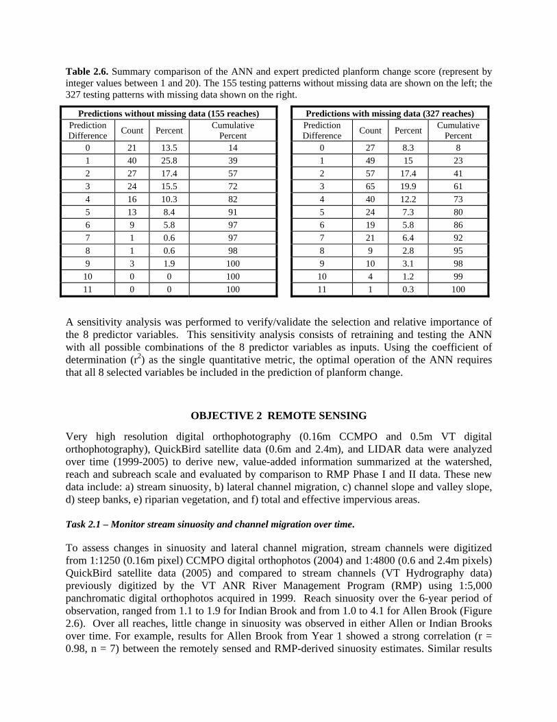
Table 2.6. Summary comparison of the ANN and expert predicted planform change score (represent by integer values between 1 and 20). The 155 testing patterns without missing data are shown on the left; the 327 testing patterns with missing data shown on the right.

Predictions without missing data (155 reaches) Predictions with missing data (327 reaches) Prediction Difference Count Percent Cumulative

Percent Prediction Difference Count Percent Cumulative

Percent 0 21 13.5 14 0 27 8.3 8 1 40 25.8 39 1 49 15 23 2 27 17.4 57 2 57 17.4 41 3 24 15.5 72 3 65 19.9 61 4 16 10.3 82 4 40 12.2 73 5 13 8.4 91 5 24 7.3 80 6 9 5.8 97 6 19 5.8 86 7 1 0.6 97 7 21 6.4 92 8 1 0.6 98 8 9 2.8 95 9 3 1.9 100 9 10 3.1 98

10 0 0 100 10 4 1.2 99 11 0 0 100 11 1 0.3 100

A sensitivity analysis was performed to verify/validate the selection and relative importance of the 8 predictor variables. This sensitivity analysis consists of retraining and testing the ANN with all possible combinations of the 8 predictor variables as inputs. Using the coefficient of determination (r2) as the single quantitative metric, the optimal operation of the ANN requires that all 8 selected variables be included in the prediction of planform change.

OBJECTIVE 2 REMOTE SENSING

Very high resolution digital orthophotography (0.16m CCMPO and 0.5m VT digital orthophotography), QuickBird satellite data (0.6m and 2.4m), and LIDAR data were analyzed over time (1999-2005) to derive new, value-added information summarized at the watershed, reach and subreach scale and evaluated by comparison to RMP Phase I and II data. These new data include: a) stream sinuosity, b) lateral channel migration, c) channel slope and valley slope, d) steep banks, e) riparian vegetation, and f) total and effective impervious areas.

Task 2.1 – Monitor stream sinuosity and channel migration over time. To assess changes in sinuosity and lateral channel migration, stream channels were digitized from 1:1250 (0.16m pixel) CCMPO digital orthophotos (2004) and 1:4800 (0.6 and 2.4m pixels) QuickBird satellite data (2005) and compared to stream channels (VT Hydrography data) previously digitized by the VT ANR River Management Program (RMP) using 1:5,000 panchromatic digital orthophotos acquired in 1999. Reach sinuosity over the 6-year period of observation, ranged from 1.1 to 1.9 for Indian Brook and from 1.0 to 4.1 for Allen Brook (Figure 2.6). Over all reaches, little change in sinuosity was observed in either Allen or Indian Brooks over time. For example, results for Allen Brook from Year 1 showed a strong correlation (r = 0.98, n = 7) between the remotely sensed and RMP-derived sinuosity estimates. Similar results

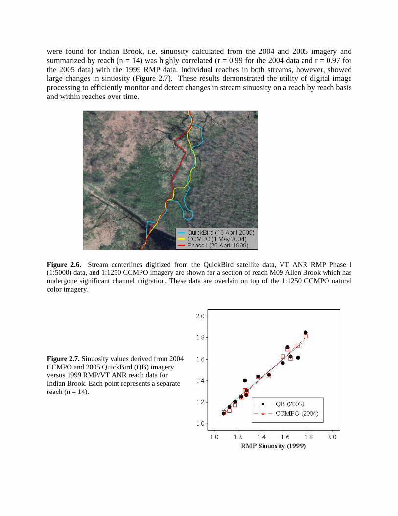
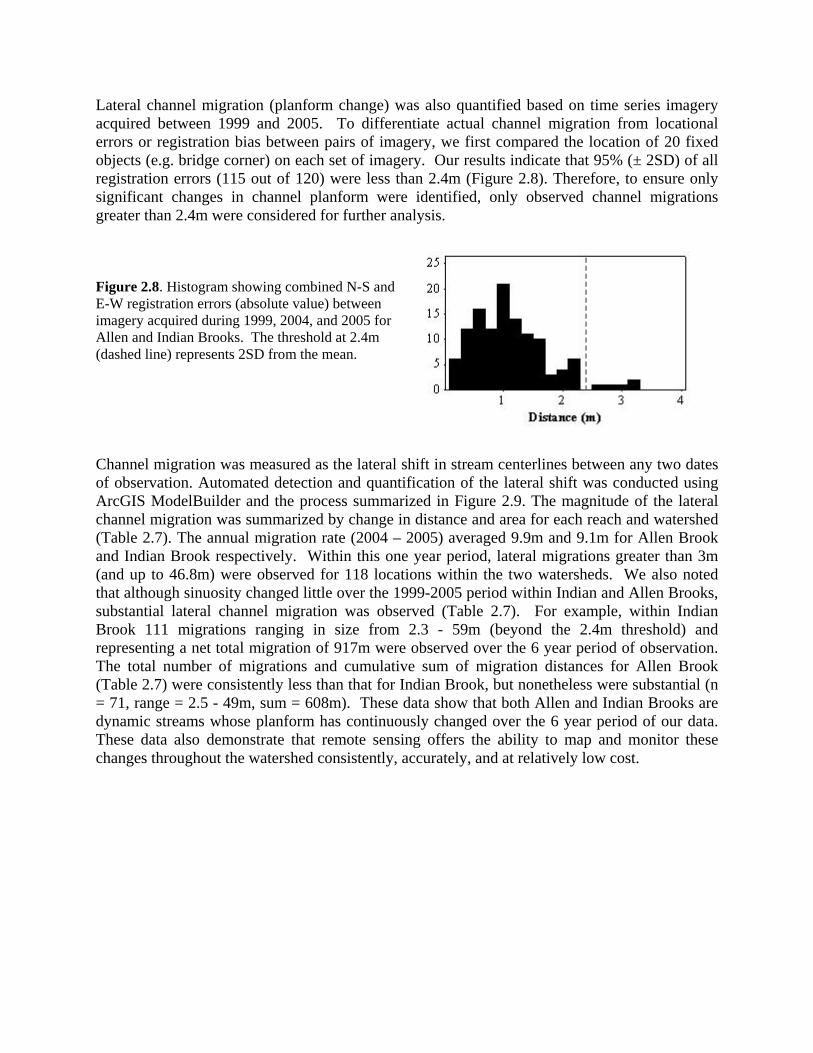
were found for Indian Brook, i.e. sinuosity calculated from the 2004 and 2005 imagery and summarized by reach (n = 14) was highly correlated (r = 0.99 for the 2004 data and r = 0.97 for the 2005 data) with the 1999 RMP data. Individual reaches in both streams, however, showed large changes in sinuosity (Figure 2.7). These results demonstrated the utility of digital image processing to efficiently monitor and detect changes in stream sinuosity on a reach by reach basis and within reaches over time.

Figure 2.6. Stream centerlines digitized from the QuickBird satellite data, VT ANR RMP Phase I (1:5000) data, and 1:1250 CCMPO imagery are shown for a section of reach M09 Allen Brook which has undergone significant channel migration. These data are overlain on top of the 1:1250 CCMPO natural color imagery.

Figure 2.7. Sinuosity values derived from 2004 CCMPO and 2005 QuickBird (QB) imagery versus 1999 RMP/VT ANR reach data for Indian Brook. Each point represents a separate reach (n = 14).

Lateral channel migration (planform change) was also quantified based on time series imagery acquired between 1999 and 2005. To differentiate actual channel migration from locational errors or registration bias between pairs of imagery, we first compared the location of 20 fixed objects (e.g. bridge corner) on each set of imagery. Our results indicate that 95% (± 2SD) of all registration errors (115 out of 120) were less than 2.4m (Figure 2.8). Therefore, to ensure only significant changes in channel planform were identified, only observed channel migrations greater than 2.4m were considered for further analysis.

Figure 2.8. Histogram showing combined N-S and

Channel migration was measured as the lateral shift in stream centerlines between any two dates

E-W registration errors (absolute value) between imagery acquired during 1999, 2004, and 2005 forAllen and Indian Brooks. The threshold at 2.4m (dashed line) represents 2SD from the mean.

of observation. Automated detection and quantification of the lateral shift was conducted using ArcGIS ModelBuilder and the process summarized in Figure 2.9. The magnitude of the lateral channel migration was summarized by change in distance and area for each reach and watershed (Table 2.7). The annual migration rate (2004 – 2005) averaged 9.9m and 9.1m for Allen Brook and Indian Brook respectively. Within this one year period, lateral migrations greater than 3m (and up to 46.8m) were observed for 118 locations within the two watersheds. We also noted that although sinuosity changed little over the 1999-2005 period within Indian and Allen Brooks, substantial lateral channel migration was observed (Table 2.7). For example, within Indian Brook 111 migrations ranging in size from 2.3 - 59m (beyond the 2.4m threshold) and representing a net total migration of 917m were observed over the 6 year period of observation. The total number of migrations and cumulative sum of migration distances for Allen Brook (Table 2.7) were consistently less than that for Indian Brook, but nonetheless were substantial (n = 71, range = 2.5 - 49m, sum = 608m). These data show that both Allen and Indian Brooks are dynamic streams whose planform has continuously changed over the 6 year period of our data. These data also demonstrate that remote sensing offers the ability to map and monitor these changes throughout the watershed consistently, accurately, and at relatively low cost.

Figure 2.9. Key steps for measuring lateral channel migration. Data for 1999 (A) and 2005 (B) imagery for reach M02 of Indian Brook are shown. Stream centerlines were digitized and then overlain (C) in ArcGIS to derive migration polygons (D; shown in blue). Only lateral shifts (indicated by arrow) greater than 2.4m were mapped to eliminate potential image registration error.

Table 2.7. Summary statistics for lateral channel migration (summarized by reach) over time along the entire lengths of Allen and Indian Brooks (units in meters). Only lateral shifts greater than 2.4m were mapped to eliminate potential image registration error.

1 Year (2004-2005) N Mean St. Dev. Median Sum Minimum MaximumAllen Brook 44 9.9 7.5 8.0 437 3.1 46.8 Indian Brook 74 9.1 5.8 7.7 675 3.2 37.3 5 Year (1999-2004) Allen Brook 57 8.3 3.4 7.7 470 2.5 18.6 Indian Brook 71 8.8 7.7 6.8 624 2.5 51.8 6 Year (1999-2005) Allen Brook 71 8.6 6.9 7.2 608 2.5 49.0 Indian Brook 111 8.3 7.3 6.3 917 2.3 58.9

Task 2.2 - Generate high spatial resolution elevation derivatives from LIDAR data, and quantify stream channel slope, valley slope, and steep banks at the reach scale.

Light Detection and Ranging (LIDAR) data provides new opportunities for the generation of accurate and detailed digital elevation models (DEM) to support improved hydrologic modeling. Processing of LIDAR data, however, is computationally intensive and processing parameters vary with investigator and objective. As such, the quality of a DEM generated from LIDAR data is dependent on the interpolation algorithm, output raster cell size, and what LIDAR information is incorporated into the processing. In this study, we employed bare earth (BE) and reflective surfaces (RS) LIDAR data with 3.2m posting that was collected over our study areas in April 2004. To determine the optimal interpolation parameters for deriving DEMs from these data, we conducted a sensitivity analysis in which select parameters known to influence the results were

systematically varied. In all, 18 digital elevation models (DEMs) were generated based on: 1) three spatial interpolation methods (inverse distance weighting (IDW), natural neighbor (NN), and ordinary kriging (OK)), 2) three different raster interpolation cell sizes (1, 2 and 3m), and 3) different data combinations, including bare earth data alone (BE) and bare earth with additional reflective surface (BERS) data. For the latter, we combined bare earth data with reflective points that were within ± 1m elevation of nearby bare earth points. The results of these 18 DEMs were then compared to elevations determined from field survey data (n = 689).

Our results demonstrated that: 1) the additional information content of the BERS data (bare earth plus reflective surfaces) best replicated known elevations and allowed the generation of smaller output raster cell sizes, and 2) NN and OK interpolations yield similarly accurate results, although NN is computationally simpler and thus executes far more quickly (Figure 2.10). More importantly, whereas OK requires geostatistical expertise, NN is easy to understand and implement. Therefore, BERS data combined with NN interpolation was found to be the best method for interpolating high resolution LIDAR data in areas with low topographic relief.

BERS NN 1m

BERS OK 2m

BERS OK 3m

BERS NN 2m

BERS OK 1m

BERS NN 3mBERS IDW

3m

BERS IDW 2m

BERS IDW 1m

BE OK 3m

BE OK 1m

BE NN 1m

BE OK 2m

BE NN 2m

BE NN 3m

BE IDW 1mBE IDW 2m

BE IDW 3m

Survey

1.0

1.5

2.0

2.5

3.0

3.5

4.0

DEMs

Figure 2.10. A comparison of interpolation algorithms, output raster cell sizes, and the addition of minimum reflective surfaces derived from LIDAR data.

Next, we compared our LIDAR-derived DEMs and slope data to elevation and slope values collected as part of VT ANR/RMP Phase I for Allen and Indian Brooks. RMP stream centerlines were used to extract a line weighted mean slope (%) from the LIDAR-derived DEM slope layer for each reach. LIDAR-derived channel slope (r = 0.99) and valley slope (r = 0.98) measurements correlated highly to Phase I RMP data for the two watersheds, individually and combined. Channel and valley slope values derived from LIDAR DEMs yielded results comparable to the Phase I RMP data quickly, efficiently, and accurately over the entire watersheds. In addition, the LIDAR-derived data provided information about changes in slope

within each reach, highlighting slope changes that do (and do not coincide) with reach boundaries. LIDAR also readily identified steep bank slopes (> 50%) which may be particularly susceptible to erosion (Figure 2.11).

Slope (%)High :

Low :

Figure 2.11. Natural color CCMPO imagery acquired in 2004 and LIDAR-derived slope for reach M01 of Allen Brook. Slopes greater than 50% are shown in red; stream centerline is shown in blue.

Task 2.3 Map total and effective impervious surface areas

Commercial high spatial resolution satellite imagery continues to offer new opportunities for improved monitoring of landscape change over time, and in particular, the ability to monitor changes in impervious surface areas associated with development that have been shown to impact fluvial processes in nearby streams. We mapped and summarized total impervious area (TIA) by reach and watershed by applying advanced object oriented classification to QuickBird satellite data. Object-oriented classification of impervious surfaces involves segmentation of pixel reflectance into homogeneous objects (i.e. polygons) followed by hierarchical decision rules for classification to differentiate impervious and pervious areas, and water (Figure 2.12). An accuracy assessment of this classification approach conducted for a nearby watershed based on 300 randomly located samples that were photointerpreted from 1:1250 CIR orthophotography with field verification demonstrated an overall mapping accuracy of 96.8%. These results, therefore, show the potential of this approach to accurately and cost effectively map impervious areas within a watershed and to monitor change over time.

Impervious surfaces Vegetated surfaces

Figure 2.12. Impervious areas derived using object oriented classification techniques based on QuickBird satellite imagery. Data from reach M03 for Allen Brook are shown. Impervious areas are shown in tan; non-impervious areas are shown in green.

Effective impervious areas (EIA), that is, those impervious areas from which surface runoff flows directly into nearby waterways, will be derived based on total impervious area (TIA), hydrologic modeling, and DEMs generated from LIDAR data. Overland flow direction and accumulation have been generated using ArcGIS hydrologic modeling tools and hydrologically-correct DEMs generated from LIDAR data to identify EIA source areas within each watershed. Riparian vegetation and, in particular, areas along streams that are without vegetation, will be incorporated within the EIA modeling. Riparian vegetation within 300 feet of the stream centerline was mapped using Definiens object oriented classification techniques incorporating high spatial resolution imagery and LIDAR digital surface models (DSM). DSMs, representing the height of objects on the earth’s surface (i.e., riparian vegetation types), were derived by subtracting the Bare Earth data from the Reflective Surface LIDAR data. Hierarchical decision rules were used to differentiate forest, shrubs, herbaceous, and bare soil within a 300 ft. riparian zone based on height and multispectral reflectance. These riparian land cover categories will determine the connectivity of impervious areas within each subwatershed to nearby streams.

Task 2.4 - Refine existing ANNs by incorporating remote sensing data In the previous research task, channel slope and valley slope (as derived from the Light Detection and Ranging (LIDAR) data have been developed, as well as sinuosity, and percent total impervious area (TIA) as derived from available Chittenden County Metropolitan Planning Organization (CCMPO) digital orthophotography and QuickBird (QB) satellite imagery. This section presents the results of sensitivity analyses performed on these four variables. Currently, two of these variables (channel and valley slope) are used in the Phase I assessment for predicting stream type. Data Coverage The Allen Brook and Indian Brook watersheds were selected for a proof-of-concept sensitivity analysis. In addition to having Phase I and Phase II assessments, these two watersheds were selected because they were included in the LIDAR, QuickBird imagery and the CCMPO digital orthophotography dataset. Allen Brook has been divided into 11 stream reaches, while Indian Brook is comprised of 17 reaches. The total 28 stream reaches used for this analysis are identified in Table 1 of Appendix B. The LIDAR survey incorporates all of the reaches that make up Allen and Indian Brook and has been used to generate new estimates of both channel and valley slope for each reach (as well as other derivatives not included in this analysis). QuickBird satellite data was available for only 23 of the 28 reaches identified in Table 1 (Appendix B) because the extent of the QuickBird scenes are based on smaller watershed boundaries defined by VT DEC Stormwater Management Division. In addition, only reaches that were classified as impaired by the state have been evaluated for TIA. Therefore, only a subset, consisting of eighteen reaches within the two watersheds that have been classified as impaired, have estimates of TIA. As a result, as variables are included into the ANN for sensitivity analysis, only the stream reaches for which all variables have been estimated were used (18 reaches highlighted in Table 1, Appendix B).

Comparison of Phase I reference stream type and Phase II stream type assessments A preliminary assessment of the differences between the stream type classifications identified during the Phase I and Phase II assessments was performed for the stream reaches associated with Allen and Indian Brook. In a Phase I assessment, reference stream types are defined for each stream reach by RMP personnel using available data (e.g. valley slope and stream confinement from existing maps). These stream type estimates are further refined using bed form and channel substrate data collected during the Phase I windshield surveys. Phase I assessment of a possible reference stream types (A, B, C, D and E of Table 2.2 – Phase I protocols) is based primarily on four channel characteristics: confinement ratio or type, valley slope, bed form and sinuosity. The assigned Phase I reference stream types are considered “provisional.” Phase II assessment of stream type involves data collected from both the Phase I assessment and the VTANR rapid geomorphic assessments (RGA). Stream type is based primarily on 6 channel characteristics: number of channel treads, entrenchment ratio, width/depth ratio, sinuosity, channel slope, and channel material. It was important in this study to note how reference stream types assigned during the Phase I assessments differ from the stream types derived during Phase II assessments. During the Phase II RGA assessments, the 28 stream reaches that comprise Allen and Indian Brook were further subdivided into 41 reaches and segments. Of these 41 reaches and segments, 13 of the Phase II stream types differed from their Phase I reference stream types. These 13 reaches and segments along with their Phase I and Phase II stream type designation are provided in Table 2.8. Again, these differences are expected as Phase I reference stream type assessments are considered provisional.

Table 2.8. Phase I reference stream type and Phase II stream type differences.

Stream Name

Phase I Reach ID

Reference Stream Type

Phase II ID

Phase II Stream Type

Allen Brook M04 C M04A F Allen Brook M04 C M04B E Allen Brook M04 C M04C E Allen Brook M04 C M04D E Allen Brook M05 C M05A E Allen Brook M07 C M07 E Allen Brook M11 E M11 F Indian Brook M09 B M09A C Indian Brook M09 B M09B F Indian Brook M11 C M11A E Indian Brook M13 E M13B B Indian Brook M16 E M16A B Indian Brook M16 E M16A B

Sensitivity analysis of select remote sensing products The following sensitivity analyses attempted to assess the added value of the remote sensing products (channel and valley slopes, sinuosity and TIA). To establish a baseline for the ANN sensitivity analyses, we developed ANNs that were trained on one watershed (one geographic region) and used for prediction on another geographic region, given a limited number of reaches (e.g. train on the original 11 reaches of Allen Brook and predict on the 17 reaches associated with Indian Brook). Figure 2.13 shows a schematic of the initial ANN trained to predict the experts’ best estimate of reference stream type given all available Phase I data (hereafter called the River Management Program or Phase I RMP ANN). The bold text in Figure 2.13 identifies the two input variables used currently in the Phase I assessment that have been derived from remote sensing data.

Figure 2.13. Schematic of inputs and outputs associated with the Phase I RMP ANN.

Since only 28 reaches were available for training and testing the ANN, two test cases were conducted. In test case 1, we trained on the 11 stream reaches of Allen Brook and made predictions for the 17 reaches associated with Indian Brook; in test case 2, we reverse the training and prediction datasets. This allows us to investigate the ANN performance using both watersheds as a training dataset and to compare predictions of reference stream type with the Phase I expert-derived evaluations. These two training scenarios produce Phase I RMP ANN estimates for reference stream type that agree with the experts for 23 of the 28 reaches. Two of the stream reaches associated with Allen Brook and three associated with Indian Brook were misclassified. See Figure 2.14. Table 2.9 lists the input data and reference stream type classifications for these five misclassified stream reaches. Given the limited number of training data, these results are encouraging with respect to the ANN’s ability to be trained on one watershed and used for prediction on another. It is important to keep in mind that only 11 Allen Brook and 17 Indian Brook reaches were used to train the Phase I RMP ANN. Table 2.9. Five stream reaches for which the Phase I RMP ANN predicted reference stream types differed from the Phase I expert assessments.

Watershed Reach ID

Confinement Ratio Bed form Valley

Slope Sinuosity Reference Stream

RMP_ANN

Allen Brook M04 6.91 Riffle-Pool 4.35 3.98 C B Allen Brook M10 9.26 Plane Bed 2.01 1.08 C E Indian Brook M12 4.88 Plane Bed 3.56 1.23 B C Indian Brook M16 3.66 Dune-Ripple 1.94 1.12 E C Indian Brook M17 73.30 Riffle-Pool 0.51 1.02 C E

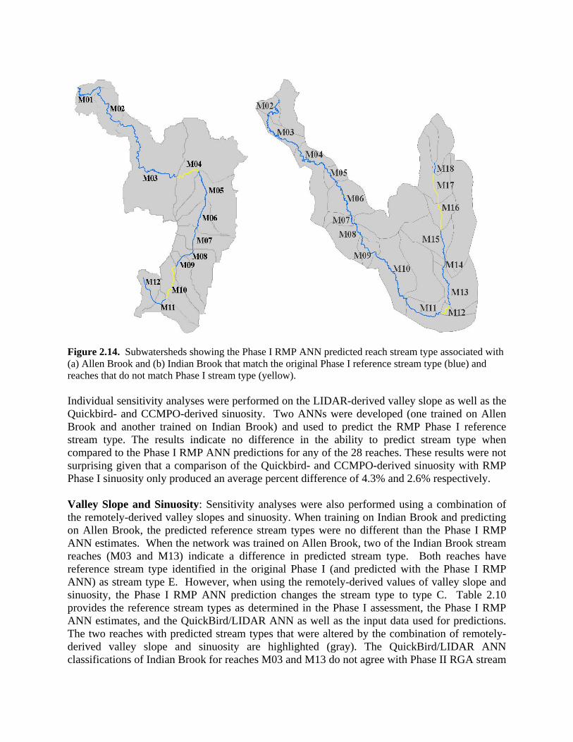
Figure 2.14. Subwatersheds showing the Phase I RMP ANN predicted reach stream type associated with (a) Allen Brook and (b) Indian Brook that match the original Phase I reference stream type (blue) and reaches that do not match Phase I stream type (yellow). Individual sensitivity analyses were performed on the LIDAR-derived valley slope as well as the Quickbird- and CCMPO-derived sinuosity. Two ANNs were developed (one trained on Allen Brook and another trained on Indian Brook) and used to predict the RMP Phase I reference stream type. The results indicate no difference in the ability to predict stream type when compared to the Phase I RMP ANN predictions for any of the 28 reaches. These results were not surprising given that a comparison of the Quickbird- and CCMPO-derived sinuosity with RMP Phase I sinuosity only produced an average percent difference of 4.3% and 2.6% respectively. Valley Slope and Sinuosity: Sensitivity analyses were also performed using a combination of the remotely-derived valley slopes and sinuosity. When training on Indian Brook and predicting on Allen Brook, the predicted reference stream types were no different than the Phase I RMP ANN estimates. When the network was trained on Allen Brook, two of the Indian Brook stream reaches (M03 and M13) indicate a difference in predicted stream type. Both reaches have reference stream type identified in the original Phase I (and predicted with the Phase I RMP ANN) as stream type E. However, when using the remotely-derived values of valley slope and sinuosity, the Phase I RMP ANN prediction changes the stream type to type C. Table 2.10 provides the reference stream types as determined in the Phase I assessment, the Phase I RMP ANN estimates, and the QuickBird/LIDAR ANN as well as the input data used for predictions. The two reaches with predicted stream types that were altered by the combination of remotely-derived valley slope and sinuosity are highlighted (gray). The QuickBird/LIDAR ANN classifications of Indian Brook for reaches M03 and M13 do not agree with Phase II RGA stream

types. In the Phase II RGA, reach M03 is still classified as an E and reach M13 has been subdivided into 4 segments, which are classified as three E’s and a B respectively. Table 2.10. Results of sensitivity analyses for Indian Brook reference stream type as determined by experts (column 9), the Phase I RMP ANN (column 10) and the remotely-derived ANN (column 11), as well as RMP and remotely-derived input data used for predictions. QuickBird satellite data is designated QB.

Water shed

Reach ID

Conf. Ratio

Bed Form

Valley Slope

LIDAR Valley Slope

Sin. QB Sin.

Ref. Stream

RMP_ANN

QB/ LIDAR

ANN Indian Brook M02 11.32 Dune-

Ripple 0.54 0.19 1.65 1.64 E E E

Indian Brook M03 3.94 Dune-

Ripple 0.30 0.75 1.62 1.71 E E C


Ripple 0.53 0.13 1.71 1.61 E E E


Ripple 0.17 0.45 1.13 1.16 E E E


Ripple 0.26 0.16 1.46 1.46 E E E


Ripple 0.47 0.30 1.77 1.85 E E E


Ripple 0.44 0.32 1.58 1.57 E E E

Indian Brook M09 2.20 Step-

Pool 3.37 3.26 1.26 1.40 B B B


Ripple 0.18 0.27 1.37 1.44 E E E

Indian Brook M11 9.13 Riffle-

Pool 0.57 0.53 1.17 1.20 C C C

Indian Brook M12 4.88 Plane

Bed 3.56 3.30 1.23 1.25 B C C


Ripple 0.52 0.68 1.27 1.27 E E C

Indian Brook M14 11.35 Riffle-

Pool 0.22 0.33 1.08 1.10 C C C


Ripple 0.53 0.30 1.27 1.32 E E E

The next step in this sensitivity analysis was the development and testing of an ANN that incorporated the remotely-derived valley slope and sinuosity, as well as the newly-derived channel slope and percent total impervious area (TIA). These four variables have been combined with the Phase I confinement ratio and bed form data and were used as inputs in a separate ANN (see schematic shown in Figure 2.15). Recall that this dataset has the most limited number of reaches (consisting of only 9 reaches in Allen and 9 in Indian Brook).

Figure 2.15. Schematic of the RMP ANN enhanced with remotely-derived input variables (shown in bold font).

Training on the 9 reaches associated with Allen Brook and predicting on the 9 reaches of Indian Brook yields identical reference stream types when compared with the Phase I RMP_ANN. When training on Indian Brook and predicting on Allen Brook, there is one reach (Allen Brook M10) that changes its predicted reference stream type (compared to Phase I RMP ANN results) from type E to C. Interestingly, this is one of the two reaches (out of 28) for which the Phase I RMP ANN misclassified the stream type as E (see Table 2.9 and Figure 2.14). Reach M10 was originally classified as a reference stream type C during both the Phase I and Phase II assessments and therefore, the Phase I RMP ANN constructed using all four remotely-derived input variables (Figure 2.15) now agrees with the Phase I and II assessments. Research to be completed Mapping of effective impervious areas is in progress. Once this final remote sensing derivative has been generated, the final task is to use our ANNs to perform sensitivity analysis incorporating all of the remote sensing data (including steep banks, riparian vegetation, lateral channel migration, and effective impervious area). We have been granted a no-cost extension to complete this final phase of the work plan. This final task will provide valuable insight into the value added utility of remote sensing products derived from the high resolution aircraft and satellite data. The expected date of completion is December, 2008.

APPENDIX A. Details of the Counterpropagation Algorithm

The counterpropagation algorithm is a supervised learning algorithm that can be used to classify data. A supervised learning algorithm is the most popular method of training ANNs to map input predictor variables to response observations. Supervised algorithms make up the majority of training algorithms for ANNs in use today. The counterpropagation algorithm maps I input predictor variables (e.g. number of bars, dominant bank vegetation, erosion length/(W/D)%, etc.) to a response variable (e.g. planform change rating/score). A set of N training patterns (composed of both predictor and response observations) is used to train the ANN. The counterpropagation algorithm requires that the response variable be categorized into K classifications or categories (e.g. 20 ratings of planform change). It is executed in two phases: a training phase and an operational phase (classification/prediction), described below in more detail.

. . .

. . .

. . .

i=1

. . .

. . .

. . .

k=1

k=2

k=K

. . .

InputLayer

. . .

Hidden Layer(Kohonen)

Output Layer(Grossberg)

RawOutput TargetInput

Vectornxnx1

*1nz

*2nz

*nJz

nz1

nz2

nJz

*ny*

1ny

*2ny

*nKy

nyny1

ny2

nKy

i=2

i=I

nx2

nIx

w11w12

w1J

wI1 wI2

wIJ

v11

v12v1K

vJ1

vJ2

vJK

∑= ijni

*nj wxz

njz 1

0

(a)

(b)

Figure 1. General schematic showing (a) architecture and notation and (b) activation function of the counterpropagation ANN. The counterpropagation architecture consists of an input layer, a “hidden” Kohonen layer, and an output Grossberg layer. Figure 1 shows a schematic of a counterpropagation ANN with I input nodes, J Kohonen hidden nodes, and K output nodes. The arcs connecting the layers of nodes have associated weights that represent the connection strength between nodes. The input-to-hidden and hidden-to-output nodal weights are known as the Kohonen (w) and Grossberg (v) weights respectively. Dual subscripts (e.g., wij) denote the weight connecting input node i and hidden node j. Therefore, each of the J hidden nodes have an associated weight vector wj comprised of I components. Likewise, the Grossberg weight matrix v is comprised of J vectors, each with K components.

Training Phase

The N training patterns are sequentially presented to train the network. The nth input vector, comprised of I predictor variables, xn = (x1

n, x2n, …xI

n), is presented to the input layer and the corresponding response observation yn is simultaneously assigned to the output layer. The input vector xn passes to the hidden layer where each hidden node computes:

(∑=

⋅=I

1iij

ni

*nj wxz ) for each Kohonen node j=1, 2,…J,

where n would equal 1 for the first training pattern. This dot product, computed for each of the J hidden nodes, represents a statistical measure of similarity between the input vector xn and the weight vector wj associated with the jth hidden node. Next, the similarity value associated with each of the J hidden nodes (represented by ) is passed through an “activation” function such that the Kohonen hidden node whose weight vector is most similar to the input vector (i.e. the “winning” node) is selected for weight adjustment. The Kohonen weight vector associated with the winning node is adjusted to be more similar to the input vector according to the following Widrow-Hoff Rule [1960] algorithm:

*njz

w jnew =

w jold + α xn − w j( )if j = winningnode,

w jold otherwise j ≠ winningnode.

⎧ ⎨ ⎪

⎩ ⎪

In the adjustment algorithm, is a learning coefficient ranging from 0 to 1 ( α =0.7 for this work), and controls the magnitude of vector adjustment and thus rate of convergence [Hecht-Nielsen, 1988]. The Widrow-Hoff adjustment ensures that only one Kohonen weight vector becomes more similar to the input vector that caused it to become activated; all others remain the same.

α

Information is then passed to the Grossberg output layer where a second dot product is computed and the raw ANN output is computed as:

(∑=

⋅=J

1jjk

nj

*nk vzy ) for k = 1, 2,…K.

The Grossberg weight vectors are adjusted according to a similar Widrow-Hoff rule: v j

v jnew =

v jold + β y n − y n*( ) if j = winning node,

v jold otherwise j ≠ winningnode .

⎧ ⎨ ⎪

⎩ ⎪

The rule is interpreted as: the updated Grossberg weight vectors equal the old Grossberg weight vectors plus some fraction, , of the difference between the raw output yβ n* and the desired observed response. A total batch of N training patterns are used to iteratively adjust the Kohonen and Grossberg weights so that subsequent network output more closely approximates the desired responses observations. One passage of all N training patterns through the ANN completes one training iteration. The root-mean-square error (RMSE) is calculated for every training iteration as:

( )K*N

yyRMSE

N

n

K

knk

*nk

2

1 1∑ ∑= =−

= ;

and provides a quantitative measure of how well the network output matches the training response observations. When the network RMSE converges to the user-defined threshold (in this work 10-6), training is complete. Thus, successful training produces a mapping between the predictor variables and the observed responses, making the ANN is ready for the classification/prediction phase.

Classification/Prediction Phase

Once trained, the Kohonen and Grossberg weight matrices become fixed and the network may be used for normal operation (classification/prediction). New input vectors consisting of patterns the ANN was not trained on are presented to the network to attain desired predictions/classifications. An additional activation function in implemented during classification/prediction to post-process the raw ANN output values to the desired classifications.

APPENDIX B. Data Available for sensitivity Analyses Table 1. Allen and Indian Brook available data.

Stream Reach ID LIDAR Derived Slopes

QuickBird/CCMPO Sinuosity

Total Impervious

Area Allen M01 Allen M02 Allen M03 Allen M04 Allen M05 Allen M06 Allen M07 Allen M08 Allen M09 Allen M10 Allen M11 Indian M02 Indian M03 Indian M04 Indian M05 Indian M06 Indian M07 Indian M08 Indian M09 Indian M10 Indian M11 Indian M12 Indian M13 Indian M14 Indian M15 Indian M16 Indian M17 Indian M18

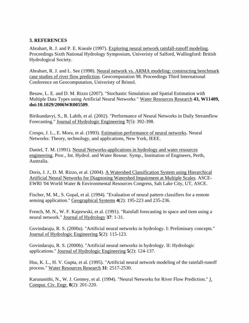
3. REFERENCES Abrahart, R. J. and P. E. Kneale (1997). Exploring neural network rainfall-runoff modeling. Proceedings Sixth National Hydrology Symposium, Univeristy of Salford, Wallingford: British Hydrological Society. Abrahart, R. J. and L. See (1998). Neural network vs. ARMA modeling: constructing benchmark case studies of river flow prediction. Geocomputation 98. Proceedings Third International Conference on Geocomputation, Univeristy of Bristol. Besaw, L. E. and D. M. Rizzo (2007). "Stochastic Simulation and Spatial Estimation with Multiple Data Types using Artificial Neural Networks " Water Resources Research 43, W11409, doi:10.1029/2006WR005509. Birikundavyi, S., R. Labib, et al. (2002). "Performance of Neural Networks in Daily Streamflow Forecasting." Journal of Hydrologic Engineering 7(5): 392-398. Crespo, J. L., E. Mora, et al. (1993). Estimation performance of neural networks. Neural Networks: Theory, technology, and applications, New York, IEEE. Daniel, T. M. (1991). Neural Networks-applications in hydrology and water resources engineering. Proc., Int. Hydrol. and Water Resour. Symp., Institution of Engineers, Perth, Australia. Doris, J. J., D. M. Rizzo, et al. (2004). A Watershed Classification System using Hierarchical Artificial Neural Networks for Diagnosing Watershed Impairment at Multiple Scales. ASCE-EWRI '04 World Water & Environmental Resources Congress, Salt Lake City, UT, ASCE. Fischer, M. M., S. Gopal, et al. (1994). "Evaluation of neural pattern classifiers for a remote sensing application." Geographical Systems 4(2): 195-223 and 235-236. French, M. N., W. F. Kajeewski, et al. (1991). "Rainfall forecasting in space and tiem using a neural network." Journal of Hydrology 37: 1-31. Govindaraju, R. S. (2000a). "Artificial neural networks in hydrology. I: Preliminary concepts." Journal of Hydrologic Engineering 5(2): 115-123. Govindaraju, R. S. (2000b). "Artificial neural networks in hydrology. II: Hydrologic applications." Journal of Hydrologic Engineering 5(2): 124-137. Hsu, K. L., H. V. Gupta, et al. (1995). "Artificial neural network modeling of the rainfall-runoff process." Water Resources Research 31: 2517-2530. Karunanithi, N., W. J. Genney, et al. (1994). "Neural Networks for River Flow Prediction." J. Comput. Civ. Engr. 8(2): 201-220.

Openshaw, S. and C. Openshaw (1997). Artificial intelligence in geography. Chichester, Wiley. Ribeiro, J., N. Lauzon, et al. (1998). "Comparison de deux modeles pour la prevision journaliere en temps reel des apports naturels." Can. J. Civ. Eng. 25(2): 291-304. Rizzo, D. M. and D. E. Dougherty (1994a). "Characterization of aquifer properties using artificial neural networks: neural kriging." Water Resources Research 30(2): 483-497. Rizzo, D. M. and D. E. Dougherty (1994b). Application of Artificial Neural Networks for Site Characterization using 'hard' and 'soft' information. Computational Methods in Water Resources X, Heidelberg, Germany. Schaap, M. G. and W. Bouten (1996). "Modeling water retention curves of sandy soils using neural networks." Water Resources Research 32(10): 3033-3040. Smith, J. and R. M. Eli (1995). "Neural-network models of rainfall-runoff processes." J. Water Resour. Plan. Manage. 121(6): 499-508. Underwood, K. L. and D. M. Rizzo (2003). Classification ANNs to Support Modeling of Sediment Transport in Geomorphically Unstable Alluvial Channels. ASCE-EWRI World Water and Environment Congress, Philadelphia, PA. VTANR (2004). Stream Geomorphic Assessment Protocols Handbooks: Remote Sensing and Field Surveys Techniques for Conducting Wateshed and Reach Level Assessments, Vermont Agency of Natural Resources. Zhu, M. L. and M. Fujita (1994). "Comparisons between fuzzy reasoning and neural network methods to forecast runoff discharge." J. Hydrosci. Hydr. Eng. 12(2): 131-141.

Phosphorus availability from the soils along two streams of theLake Champlain Basin: mapping, characterization and seasonal mobility

Basic Information

Title: Phosphorus availability from the soils along two streams of the Lake ChamplainBasin: mapping, characterization and seasonal mobility



End Date: 2/29/2008



Research Category: Water Quality

Focus Category: Nutrients, Non Point Pollution, Water Quality

Descriptors:

Principal Investigators: Donald Ross, Joel P. Tilley

Publication1. Young, E.O., D.S. Ross, J.P. Tilley, K. Underwood, C. Alves, and T. Villars. 2006. Phosphorus

availability along two small streams in Vermont: Mapping, characterization and potential mobility.ASA-CSA-SSSA Annual Meeting. Indianapolis, IN. In Agronomy Abstracts.

2. Alves, C., E.O. Young, and D.S. Ross. 2007. Phosphorus availability in some Vermont floodplainsoils. ASA-CSA-SSSA Annual Meeting. New Orleans, LA. In Agronomy Abstracts.

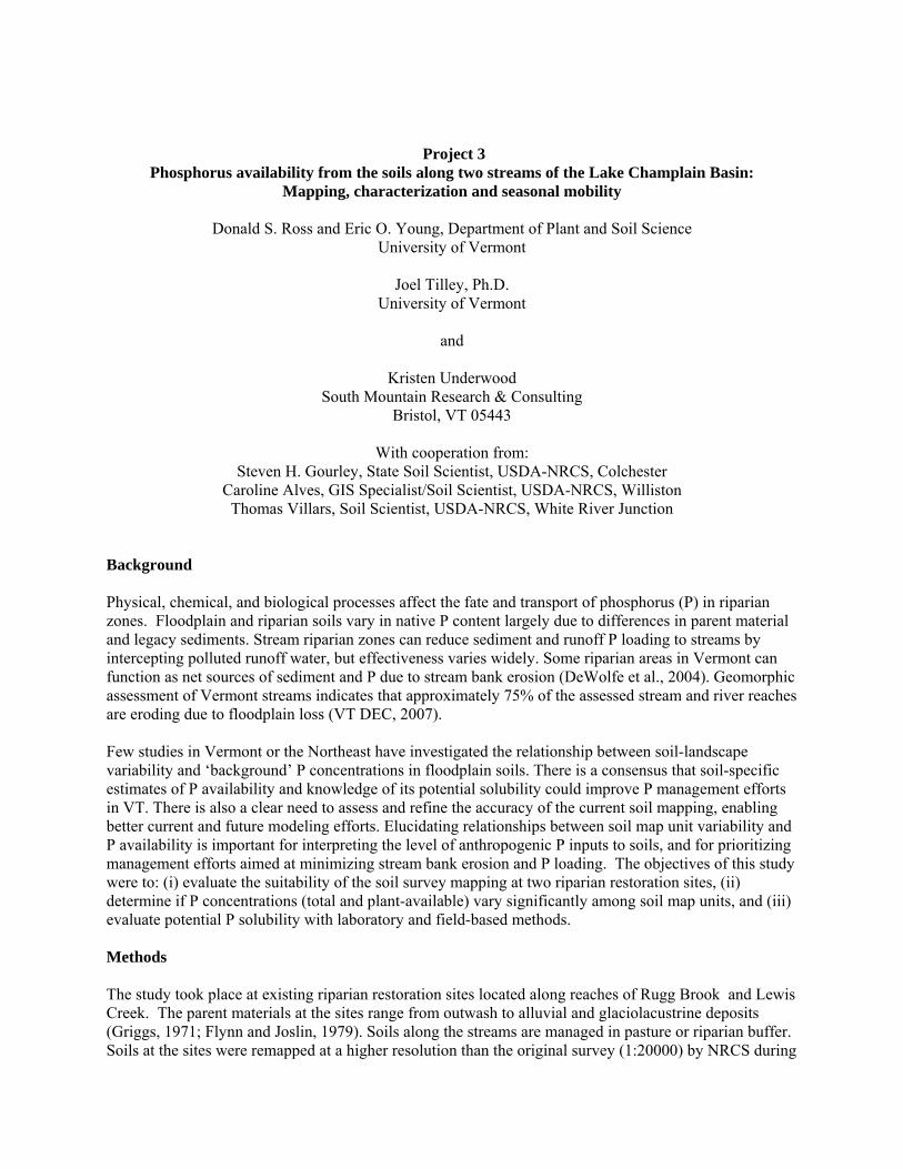
Project 3

Phosphorus availability from the soils along two streams of the Lake Champlain Basin: Mapping, characterization and seasonal mobility

Donald S. Ross and Eric O. Young, Department of Plant and Soil Science


Joel Tilley, Ph.D. University of Vermont

and

Kristen Underwood

South Mountain Research & Consulting Bristol, VT 05443

With cooperation from:

Steven H. Gourley, State Soil Scientist, USDA-NRCS, Colchester Caroline Alves, GIS Specialist/Soil Scientist, USDA-NRCS, Williston

Thomas Villars, Soil Scientist, USDA-NRCS, White River Junction Background Physical, chemical, and biological processes affect the fate and transport of phosphorus (P) in riparian zones. Floodplain and riparian soils vary in native P content largely due to differences in parent material and legacy sediments. Stream riparian zones can reduce sediment and runoff P loading to streams by intercepting polluted runoff water, but effectiveness varies widely. Some riparian areas in Vermont can function as net sources of sediment and P due to stream bank erosion (DeWolfe et al., 2004). Geomorphic assessment of Vermont streams indicates that approximately 75% of the assessed stream and river reaches are eroding due to floodplain loss (VT DEC, 2007). Few studies in Vermont or the Northeast have investigated the relationship between soil-landscape variability and ‘background’ P concentrations in floodplain soils. There is a consensus that soil-specific estimates of P availability and knowledge of its potential solubility could improve P management efforts in VT. There is also a clear need to assess and refine the accuracy of the current soil mapping, enabling better current and future modeling efforts. Elucidating relationships between soil map unit variability and P availability is important for interpreting the level of anthropogenic P inputs to soils, and for prioritizing management efforts aimed at minimizing stream bank erosion and P loading. The objectives of this study were to: (i) evaluate the suitability of the soil survey mapping at two riparian restoration sites, (ii) determine if P concentrations (total and plant-available) vary significantly among soil map units, and (iii) evaluate potential P solubility with laboratory and field-based methods. Methods The study took place at existing riparian restoration sites located along reaches of Rugg Brook and Lewis Creek. The parent materials at the sites range from outwash to alluvial and glaciolacustrine deposits (Griggs, 1971; Flynn and Joslin, 1979). Soils along the streams are managed in pasture or riparian buffer. Soils at the sites were remapped at a higher resolution than the original survey (1:20000) by NRCS during

2006. The new map unit delineations were hand-drawn based on field profile sampling and interpretation of stereo imagery, and subsequently digitized. Soil samples for chemical analysis were taken at 15 cm depth intervals to a depth of ~1 m at twenty locations distributed across each site. Samples were taken from discrete map units based on the remapping by NRCS. Most map units were sampled at 4 to 6 locations. Samples were taken at two locations spaced approximately 3-5 m apart in random directions, and composited for analysis. Care was taken to ensure that the subsamples were from the same map unit. Sediment samples for chemical analysis were taken from established cross-sections for geomorphic assessment at the Lewis Creek site, and included channel, bed, and stream bank sediments. Soil and Water Analyses Soils were sieved and dried prior to chemical analysis. Available P and cations were determined by extraction (1:5) with ammonium acetate buffered at pH 4.8 (the Modified Morgan extractant). Phosphorus in the extract was measured by a spectrophotometer with the molybdate stannous chloride method. Organic matter was determined by loss on ignition. Total P and cations were determined by nitric acid digestion in a microwave accelerated reaction system. Extracts were diluted and P and metals were measured by Inductively Coupled Plasma-Optical Emission Spectroscopy using standard techniques. Subsets of soils were analyzed for distilled water extractable (1:25) inorganic P, and for organic and inorganic water extractable (1:4) P. A subset of soils was collected in late November 2007 for determining P release under flooded conditions. Microcosms were constructed according to Young and Ross (2001). Field moist samples were flooded for 75 days with distilled water and porewater and floodwater were periodically monitored for molybdate reactive P and soluble iron. Soluble iron (Fe2+) was measured colorimetrically (Jackson, 1958). Air-dried subsamples of soil used in the microcosm experiment were extracted with water and assayed for total soluble organic P and P hydrolyzed by phosphatase enzymes. Total P in water extracts was measured using the persulfate oxidation method. Enzyme assays were done according to the method of Turner et al. (2002). During the 2007 field season, duplicate porous cup tension lysimeters (25 cm deep) were installed at four locations at each site that differed in soil and/or sediment properties (locations not shown). Vacuum was applied (50 kPa) to lysimeters after significant rainfall events and samples were extracted after 24 to 48 hr of equilibration. Soil water samples were analyzed for molybdate reactive P. Statistical Methods A General Linear Modeling approach was used for hypothesis testing and variance explanation (SAS, 1999). Analysis of Variance was used to test the null hypothesis of equivalent soil P concentrations among map units. One-way ANOVA was used for individual series to test for differences among depths. Means were separated by a priori linear contrasts using least square. Residuals from each analysis were inspected to check for gross violations of GLM assumptions. Stepwise multiple linear regression was applied to explore relationships among total P concentrations and soil physical and chemical properties. Results and Discussion Mapping The Rugg Brook study area was originally mapped entirely as Binghamville silt loam (Flynn and Joslin, 1979). Following our high intensity remapping, five additional soil series were identified and mapped (Fig. 3.1). Rather than being all silt loam, soils on the north side of the stream varied from sandy outwash (Windsor), to silty clay deposits (Covington) to the west. Following the high intensity remapping, the stream bank soils were mapped as the Winooski series (very fine sandy loam formed in recent alluvium),

as opposed to a glaciolacustrine silt loam (e.g., Binghamville). The fact that these soils differ in both drainage and texture could be an important distinction depending on the objective. In terms of P

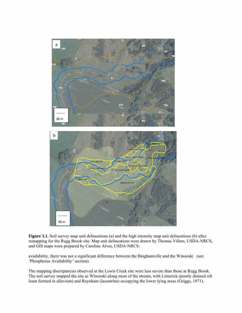
Figure 3.1remappingand GIS m

availability‘Phosphoru The mappiThe soil suloam form

_____

60 m

a

. So foraps

, ths A

ng rveed i

b

il survey map unit delineations (a) and the high intensity map unit delineations (b) after the Rugg Brook site. Map unit delineations were drawn by Thomas Villars, USDA-NRCS, were prepared by Caroline Alves, USDA-NRCS.

_____

60 m

ere was not a significant difference between the Binghamville and the Winooski (see vailability’ section).

discrepancies observed at the Lewis Creek site were less severe than those at Rugg Brook. y mapped the site as Winooski along most of the stream, with Limerick (poorly drained silt n alluvium) and Raynham (lacustrine) occupying the lower lying areas (Griggs, 1971).

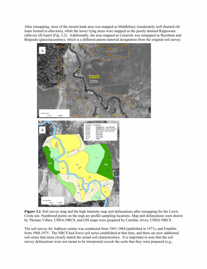
After remapping, most of the stream bank area was mapped as Middlebury (moderately well drained silt loam formed in alluvium), while the lower lying areas were mapped as the poorly drained Rippowam (alluvial silt loam) (Fig. 3.2). Additionally, the area mapped as Limerick was remapped as Raynham and Belgrade (glaciolacustrine), which is a different parent material designation from the original soil survey. FigureCreek sby Tho The soifrom 19soil sersurvey

57 m 1:2870

3.2itema

l su68

ies del

b

a

40 m 1:2000

. Soil survey map and the high intensity map unit delineations after remapping for the Lewis . Numbered points on the map are profile sampling locations. Map unit delineations were drawn s Villars, USDA-NRCS, and GIS maps were prepared by Caroline Alves, USDA-NRCS.

rvey for Addison county was conducted from 1941-1964 (published in 1971), and Franklin -1975. The NRCS had fewer soil series established at that time, and there are now additional that more closely match the actual soil characteristics. It is important to note that the soil ineations were not meant to be interpreted outside the scale that they were prepared (e.g.,

1:20000). In general, the minimum map unit delineation area is about 3 acres when mapping at the 1:20000 scale. Thus, a certain degree of error was expected because the field characterization we did permitted map units to be delineated at a finer resolution than the original survey. The practical significance of the mapping discrepancies we observed at the two sites will vary depending on the objective. It is difficult to place the mapping discrepancies into context, since no other studies in Vermont have compared 1:20000 mapping to higher intensity delineations. Map Unit Delineations in the Riparian Corridors Additional soil sampling and map unit verification took place during the summer of 2007. Approximately twenty map units were sampled between the two corridors. Soil pit excavation, sampling, and profile descriptions were done according to USDA-NRCS guidelines for submitting samples to the National Soil Survey Laboratory. After the National Laboratory has completed all analyses, NRCS will be able to determine how well the taxonomy of the mapped series (e.g., the soil survey map unit delineations) matches the taxonomy of pedon samples taken within the corridors. This information will enable a broader scale evaluation of how well the current soil survey mapping is within the corridors. To date, we have only received preliminary data for a few of the map units. These data include detailed chemical and physical properties and measures of total and available P forms (we anticipate the arrival of the full data set by summer 2008). Caroline Alves of the USDA-NRCS will be compiling data from the National Laboratory, and these data will eventually be available on-line to the public. Based on preliminary soil descriptions, the agreement between the soil survey map unit delineations and the soils sampled in the field was inconsistent. In some areas map unit properties appeared to match the survey descriptions well, whereas other locations clearly differed. Due to the high variability of the soils and the length of time required to sample and describe each pedon, intensive sampling along individual stream reaches was not possible. Therefore, additional sampling would be required to remap extensive areas outside of the restoration sites. Soil Phosphorus Availability among Map Units Plant-available P (hereafter referred to as ‘available P’) concentrations were generally low (relative to the University of Vermont field crop guidelines for P), while total P concentrations ranged widely (Table 3.1). Most of the available P concentrations were in the low to medium range (0.5 to 3.5 mg kg-1), with some in the optimum and high range (4.1 to 7.0 and 7.1 to 20 mg kg-1, respectively). Significant effects were observed on available P when all depths were grouped by series (p<.0001) and drainage (p =.0007), but were weakly related to parent material (p =.06) and unrelated with depth (p = .36). In contrast, all of these factors had a significant (p≤.0001) effect on total P concentration, suggesting that total P variation was more closely related to the landscape than available P. Total P varied significantly among depths for most of the map units, with greater total P levels in Ap horizons (Table 3.2). For the Covington and Belgrade series, total P was greatest in the C horizon. Available P levels did not tend to change substantially with depth (Table 3.2). There was only one soil (Belgrade) where the hypothesis of equivalent available P levels with depth was rejected (p =.06). The more imperfectly drained soils tended to have greater available and total P (Table 3.2). The Raynham and Rippowam map units had significantly greater available and total P relative to other soils. This could be related to the fact that the more poorly drained soils had a greater proportion of silt and clay, which contributes to a greater capacity to bind metal cations (and thus P) relative to coarser textured soils.

Table 3.1. Summary statistics for select soil chemical properties for all samples taken at the sites. Soil property n Mean SD Minimum MaximumpH 297 6.1 0.7 4.9 7.6Organic matter (g kg-1) 297 20.0 15.0 2.0 95.0Available P (mg kg-1)‡ 297 1.7 1.4 0.3 9.2Available Al 297 48.9 44.5 5.0 296.0Available Fe 297 12.9 19.4 1.4 185.9Available Mn 297 5.4 8.4 0.0 69.8Available Ca 297 772.4 509.6 49.0 2169.0Available K 297 32.8 26.1 10.9 314.1Available Mg 297 106.8 74.2 8.0 331.9Total P (mg kg-1) ‡‡ 295 552 208 109 1360Total Al 295 12126 3762 4490 23800Total Fe 295 19393 4425 10200 36000Total Mn 294 365 181 87 1040Total Ca 295 2528 1000 484 6850Total K 295 1536 684 429 4500Total Mg 295 4250 1145 2050 8610

‡ The Vermont soil test (e.g., available P and cations) is 1.25 M ammonium acetate buffered at pH = 4.8 ‡‡ Total element analysis was done by EPA Method 3051a. Approximately 80% of the P was recovered from a NIST certified reference standard. Recovery of P and other elements is typically greater for more exhaustive methods (e.g., sodium carbonate fusion, hydrofluoric acid, sulfuric acid). Table 3.2. Mean total and available phosphorus concentrations for the soil map units sampled. Total P Available P Total P Available P Total P Available P Depth Belgrade (n = 4) Binghamville (n = 4) Covington (n = 4) ----------------------------------------------------mg kg-1---------------------------------------------------- 0–15 437 ab‡ 0.87a 687 a 1.18 531 a 1.35 91‡‡ 0.09 68 0.19 99 0.29 15–30 305 a 0.70a 589 ab 0.93 390 ab 0.60 51 0.07 38 0.24 80 0.09 30–45 283 a 0.88a 536 ab 0.98 292 b 0.80 63 0.17 44 0.25 40 0.12 45–60 509 ab 0.98a 548 ab 1.08 227 b 0.98 201 0.21 79 0.26 40 0.28 60–75 519 ab 1.65 b 504 ab 0.90 413 ab 1.15 42 0.45 95 0.19 139 0.30 75–90 559 ab 2.18b 499 ab 1.43 596 a 1.40 18 0.54 78 0.37 128 0.44 90–105 601 b 2.18b 482 b 1.73 631 a 1.58 53 0.58 55 0.38 109 0.61

‡Means within a series (e.g., across depths intervals) with different letters are different at p≤ 0.05 ‡‡ Standard error of the mean

Table 3.2. Continued Total P Available P Total P Available P Total P Available P Depth Limerick (n = 5) Middlebury (n = 5) Raynham (n = 6) -----------------------------------------mg kg-1----------------------------------------- 0–15 787 a 1.12 646 a 1.53 925 a 3.78 140 0.15 48 0.29 104 1.16 15–30 695 ab 1.00 569 ab 1.68 810 ab 2.50 141 0.18 29 0.43 136 0.97 30–45 570 ab 0.94 498 b 1.43 666 b 3.36 144 0.33 34 0.17 65 1.48 45–60 476 b 0.74 536 b 1.83 636 b 3.62 69 0.07 33 0.14 52 1.34 60–75 500 ab 0.86 560 ab 1.52 645 b 3.84 50 0.26 25 0.15 39 0.98 75–90 480 ab 0.82 564 ab 1.38 673 b 3.80 44 0.10 35 0.11 42 1.15 90–105 488 b 1.04 543 ab 1.73 648 b 3.69 32 0.21 47 0.23 47 1.00

Table 3.2. Continued Total P Available P Total P Available P Total P Available P Depth Rippowam (n = 5) Wappinger (n = 2) Winooski (n = 5) -----------------------------------------mg kg-1----------------------------------------- 0–15 839 a 2.42 540 0.80 656 a 1.72 33 0.29 19 0.30 50 0.23 15–30 829 ab 1.82 474 0.50 585 ab 1.14 108 0.40 42 0.10 59 0.15 30–45 750 ab 1.86 426 0.45 469 b 1.08 81 0.60 75 0.15 44 0.22 45–60 732 ab 2.03 461 0.60 455 b 1.00 59 0.35 155 0.20 83 0.32 60–75 674 ab 2.50 444 0.60 460 b 1.06 56 0.37 97 0.20 96 0.18 75–90 561 b 2.40 436 0.55 465 b 1.22 78 0.36 27 0.05 58 0.20 90–105 598 b 2.05 424 0.60 455 b 1.36 69 0.46 3 0.20 52 0.14

Factors Affecting Total Phosphorus Concentrations Available P was significantly correlated (r = 0.40, p<.0001) with total P concentrations across all depths (Fig. 3.3). The strength of this correlation generally increased when soils were grouped by series or depth.

Besides the notable correlation with total P, available P showed weak correlations with other minerals. Total P was significantly correlated with total Ca (r = 0.58, p<.0001), total Fe (r = 0.40, p<.0001), and organic matter (r = 0.44, p<.0001) across the data set (Fig. 3.3). Stepwise multiple linear regression revealed that available P, total Ca, and pH jointly explained 58% of the total P variation (Fig. 3.3). This suggests that the combination of increasing soil Ca levels and labile inorganic P strongly influenced total P concentrations. Two of the three outliers were from the same soil profile and had high total Ca (5700 and 6850 mg kg-1) and anomalously low total P (355 and 418 mg kg-1) relative to the average. The stepwise procedure was also performed for different depths. The best model was for the 0-30cm samples (with total Ca, available P, and pH as predictors) (Fig. 3.3). However, predictability dropped for other

0

400

800

1200

1600

0 2 4 6 8 10

Total P(mg kg-1)

Soil test P (mg kg-1)

r = 0.40p<.0001

1600

0

400

800

1200

1600

0 5000 10000

Total P(mg kg-1)

Total calcium (mg kg-1)

r = 0.58p<.0001

Figure 3.3. Relationship between total P anorganic matter (c), and total P and total ironpredicted total P with total Ca, available P,observed and predicted total P using the sam

0

400

800

1200

1600

0 20 40 60 80 100

Total P(mg kg-1)

Soil organic matter (g kg-1)

r = 0.44p<.0001

y = 0.591x + 223.1R² = 0.58, p<.0001

0

400

800

1200

1600

0 400 800 1200 1600

Predicted tal Pg kg-1)

Observed total P (mg kg-1)

to(m

a

d available P (a), total P and tota (d) for all samples. Relationship

and pH as independent variablese independent variables for all

0

400

800

1200

0 10000 20000 300

Total P(mg kg-1)

Total iron (mg k

y = 0.765xR² = 0.77 p

0

400

800

1200

1600

0 400 800 1

Predicted total P

(mg kg-1)

Observed total P (m

b

c
d
00 40000

g-1)

r = 0.40p<.0001

e
f
l calcium (b), total P and soil between observed and

(e). Relationship between 0-30 cm samples (f).

+ 147.8<.0001

200 1600

g kg-1)

depths. For example, total Ca independently explained 39% of total variation, while other metals showed weak relationships. Total Fe was selected as the only significant (p<.0001) predictor of total P for the 45-60 and 75-90 cm sampling depths. Grouping soils by series also confirmed the importance of total Ca, but other variables were significant. For example, organic matter content independently explained 58% of the total P variation for all of the Raynham samples, whereas total K and organic matter jointly explained 76% of total P variation for the Winooski samples. These results suggest that other minerals and factors related to organic matter, drainage, and texture are also associated with total P variation. The consistently strong relationship between total P and Ca suggests that Ca minerals or compounds (e.g., apatite or other Ca-P associations) could be an important source of P (the use of direct analytical methods such as x-ray spectroscopy and diffraction would be required to confirm this). A subset of profile samples (n =74) was selected to further study the relation between soil properties and P availability. Profile samples were selected to provide a range of properties to reflect the predominant map units along the streams. For these samples, total P was significantly correlated with silt content (r = 0.73, p<.0001), soil water content (r = 0.68, p<.0001), and organic matter (r = 0.54, p<.0001) (Fig. 3.4). Stepwise regression selected silt content, organic matter, available P, and Al as significant (R2=0.71, p<.01) predictors (data not shown). There were also significant correlations between silt and soil water content (r = 0.70, p<.0001), silt and organic matter content (r = 0.49, p<.0001), and between organic matter and water content (r = 0.68, p<.0001). These relationships suggest that more poorly drained, fine-textured soils developed greater total P concentrations. From a pedology perspective, this is plausible because finer textured-soils in this study were associated with the lower-lying areas, where finer particles tend to collect on the landscape. Wetter soils tend to have greater organic carbon which could contribute to greater organic P concentrations, and finer-textured soils can also bind greater quantities of metals (and thus P) relative to coarser textured soils due to their greater surface area and number of exchange sites. Figure 3.4. Relationship between total P and silt content (a), total P and soil water content (b), silt content and soil water content (c), and organic matter and soil water content (d) for a subset of profile samples

0

200

400

600

800

1000

1200

1400

0 20 40 60 80 100

Total P (mg kg-1)

Silt content (%)

r = 0.73p<.0001

0

200

400

600

800

1000

1200

1400

0 20 40

Total P(mg kg-1)

Soil water content (%)

r = 0.68p <.0001

60

ba

0

20

40

60

80

100

0 20 40 60

Silt content

(%)


r = 0.70p<.0001

c

0

20

40

60

80

100

0 20 40 6

Soil organic matter

content (g kg-1)

0


r = 0.68p<.0001

d

(n = 74) collected at the riparian restoration sites.

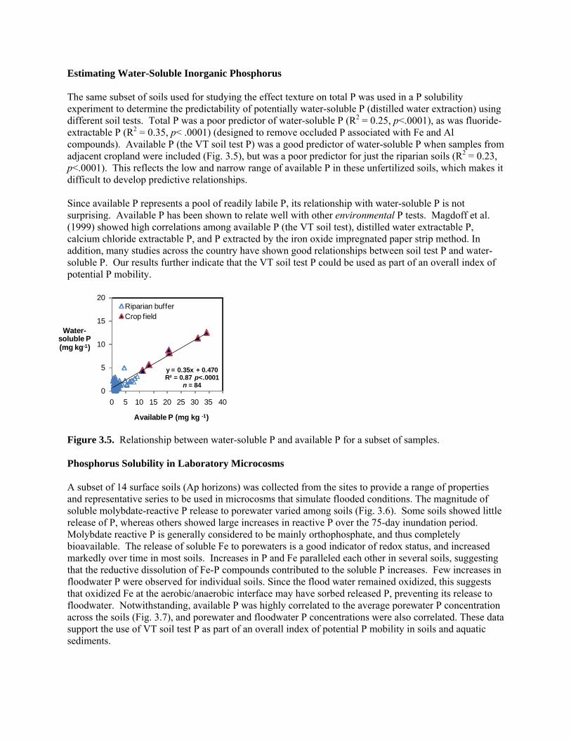
Estimating Water-Soluble Inorganic Phosphorus The same subset of soils used for studying the effect texture on total P was used in a P solubility experiment to determine the predictability of potentially water-soluble P (distilled water extraction) using different soil tests. Total P was a poor predictor of water-soluble P (R2 = 0.25, p<.0001), as was fluoride-extractable P (R2 = 0.35, p< .0001) (designed to remove occluded P associated with Fe and Al compounds). Available P (the VT soil test P) was a good predictor of water-soluble P when samples from adjacent cropland were included (Fig. 3.5), but was a poor predictor for just the riparian soils (R2 = 0.23, p<.0001). This reflects the low and narrow range of available P in these unfertilized soils, which makes it difficult to develop predictive relationships. Since available P represents a pool of readily labile P, its relationship with water-soluble P is not surprising. Available P has been shown to relate well with other environmental P tests. Magdoff et al. (1999) showed high correlations among available P (the VT soil test), distilled water extractable P, calcium chloride extractable P, and P extracted by the iron oxide impregnated paper strip method. In addition, many studies across the country have shown good relationships between soil test P and water-soluble P. Our results further indicate that the VT soil test P could be used as part of an overall index of potential P mobility.

y = 0.35x + 0.470R² = 0.87 p<.0001

n = 840

5

10

15

20

0 5 10 15 20 25 30 35 40

Water-soluble P (mg kg-1)

Available P (mg kg -1)

Riparian bufferCrop field

Figure 3.5. Relationship between water-soluble P and available P for a subset of samples. Phosphorus Solubility in Laboratory Microcosms A subset of 14 surface soils (Ap horizons) was collected from the sites to provide a range of properties and representative series to be used in microcosms that simulate flooded conditions. The magnitude of soluble molybdate-reactive P release to porewater varied among soils (Fig. 3.6). Some soils showed little release of P, whereas others showed large increases in reactive P over the 75-day inundation period. Molybdate reactive P is generally considered to be mainly orthophosphate, and thus completely bioavailable. The release of soluble Fe to porewaters is a good indicator of redox status, and increased markedly over time in most soils. Increases in P and Fe paralleled each other in several soils, suggesting that the reductive dissolution of Fe-P compounds contributed to the soluble P increases. Few increases in floodwater P were observed for individual soils. Since the flood water remained oxidized, this suggests that oxidized Fe at the aerobic/anaerobic interface may have sorbed released P, preventing its release to floodwater. Notwithstanding, available P was highly correlated to the average porewater P concentration across the soils (Fig. 3.7), and porewater and floodwater P concentrations were also correlated. These data support the use of VT soil test P as part of an overall index of potential P mobility in soils and aquatic sediments.

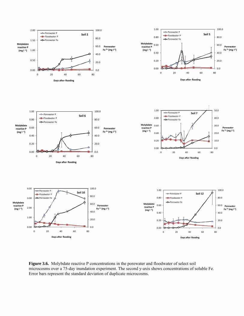
ganic Phosphorus Figure 3.6. Molybdate reactive P concentrations in the porewater and floodwater of select soil microcosms over a 75-day inundation experiment. The second y-axis shows concentrations of soluble Fe. Error bars represent the standard deviation of duplicate microcosms.

0.0

20.0

40.0

60.0

80.0

100.0

0.00

0.50

1.00

1.50

2.00

0 20 40 60 80

PorewaterFe 2+ (mg l‐1)

Molybdatereactive P(mg l ‐1)

Days after flooding

Porewater PFloodwater P

Porewater Fe

Soil 2

0.0

20.0

40.0

60.0

80.0

100.0

0.00

0.20

0.40

0.60

0.80

1.00

0 20 40 60 80


Molybdate reactive P(mg l ‐1)

Days after flooding

Porewater P

Floodwater P

Porewater Fe

Soil 5

0.0

20.0

40.0

60.0

80.0

100.0

0.00

20

40

60

80

00

0 20 40 60 80



Days after flooding

Porewater P

Floodwater P

Porewater Fe

Soil 6

0.0

10.0

20.0

30.0

40.0

50.0

0.00

0.20

0.40

0.60

0.80

1.00

0 20 40 60 80



Days after flooding

Porewater P

Floodwater P

Porewater Fe

Soil 71.

0.

0.

0.

0.

0.0

20.0

40.0

60.0

80.0

100.0

0.00

1.00

2.00

3.00

4.00

0 20 40 60 80



Days after flooding

0.0

20.0

40.0

60.0

80.0

100.0

0.00

0.20

0.40

0.60

0.80

1.00

0 20 40 60 80



Days after flooding

Porewater P

Floodwater P

Porewater Fe

Soil 12

Porewater P

Floodwater P

Porewater Fe

Soil 10

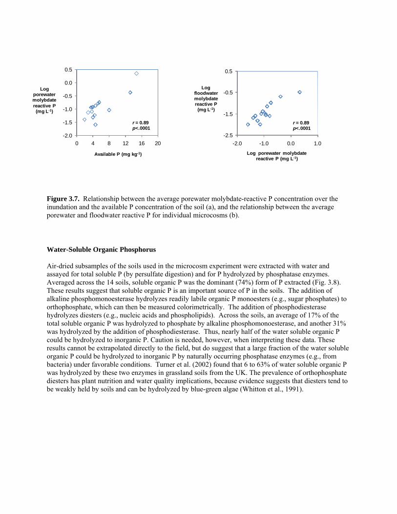
-2.0

-1.5

-1.0

-0.5

0.0

0.5

0 4 8 12 16 20

Log porewater molybdate reactive P (mg L-1)

Available P (mg kg-1)

r = 0.89p<.0001

-2.5

-1.5

-0.5

0.5

-2.0 -1.0 0.0 1.0

Log floodwater molybdate reactive P (mg L-1)

Log porewater molybdate reactive P (mg L-1)

r = 0.89p<.0001

Figure 3.7. Relationship between the average porewater molybdate-reactive P concentration over the inundation and the available P concentration of the soil (a), and the relationship between the average porewater and floodwater reactive P for individual microcosms (b). Water-Soluble Organic Phosphorus Air-dried subsamples of the soils used in the microcosm experiment were extracted with water and assayed for total soluble P (by persulfate digestion) and for P hydrolyzed by phosphatase enzymes. Averaged across the 14 soils, soluble organic P was the dominant (74%) form of P extracted (Fig. 3.8). These results suggest that soluble organic P is an important source of P in the soils. The addition of alkaline phosphomonoesterase hydrolyzes readily labile organic P monoesters (e.g., sugar phosphates) to orthophosphate, which can then be measured colorimetrically. The addition of phosphodiesterase hydrolyzes diesters (e.g., nucleic acids and phospholipids). Across the soils, an average of 17% of the total soluble organic P was hydrolyzed to phosphate by alkaline phosphomonoesterase, and another 31% was hydrolyzed by the addition of phosphodiesterase. Thus, nearly half of the water soluble organic P could be hydrolyzed to inorganic P. Caution is needed, however, when interpreting these data. These results cannot be extrapolated directly to the field, but do suggest that a large fraction of the water soluble organic P could be hydrolyzed to inorganic P by naturally occurring phosphatase enzymes (e.g., from bacteria) under favorable conditions. Turner et al. (2002) found that 6 to 63% of water soluble organic P was hydrolyzed by these two enzymes in grassland soils from the UK. The prevalence of orthophosphate diesters has plant nutrition and water quality implications, because evidence suggests that diesters tend to be weakly held by soils and can be hydrolyzed by blue-green algae (Whitton et al., 1991).

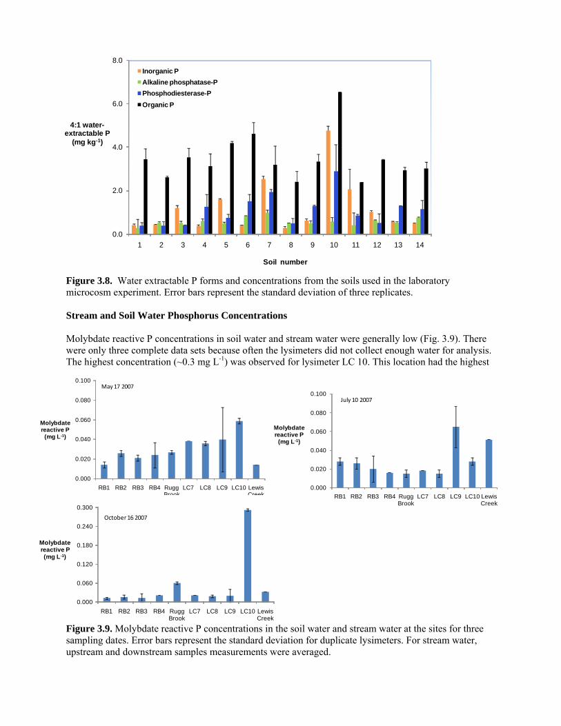
Figure 3.8. Water extractable P forms and concentrations from the soils used in the laboratory microcosm experiment. Error bars represent the standard deviation of three replicates. Stream and Soil Water Phosphorus Concentrations Molybdate reactive P concentrations in soil water and stream water were generally low (Fig. 3.9). There were only three complete data sets because often the lysimeters did not collect enough water for analysis. The highest concentration (~0.3 mg L-1) was observed for lysimeter LC 10. This location had the highest Figure 3.9. Molybdate reactive P concentrations in the soil water and stream water at the sites for three sampling dates. Error bars represent the standard deviation for duplicate lysimeters. For stream water, upstream and downstream samples measurements were averaged.

0.000

0.020

0.040

0.060

0.080

0.100

RB1 RB2 RB3 RB4 Rugg Brook

LC7 LC8 LC9 LC10 Lewis Creek

Molybdatereactive P

(mg L-1)

July 10 2007

0.000

0.020

0.040

0.060

0.080

0.100



Molybdatereactive P

(mg L-1)

May 17 2007

0.0

2.0

4.0

6.0

8.0

1 2 3 4 5 6 7 8 9 10 11 12 13 14

4:1 water-extractable P

(mg kg-1)

Soil number

Inorganic PAlkaline phosphatase-PPhosphodiesterase-POrganic P

0.000

0.060

0.120

0.180

0.240

0.300



Molybdatereactive P(mg L-1)

October16 2007

available P of all the map units sampled (Raynham), and the greatest TP concentration (1360 mg kg-1 at the 15-30 cm depth). There was no significant correlation between available P and the average soil water P concentration. This has been found by other studies and probably related to the limited range of P values in this data set. Although these concentrations are generally low, they are in the range of dissolved P concentrations that have been associated with the eutrophication of surface water (e.g., 0.01 to 0.03 mg P L-1). Phosphorus Availability of Stream Sediments The average total and available P concentrations (507 and 1.5 mg kg-1, respectfully) of the stream sediments were slightly lower than the grand mean of all the soil samples (552 and 1.7 mg kg-1, respectively). In terms of plant availability and potential solubility, these are low values. However, the flooding experiments showed that soils relatively low in P status may still release P under reducing conditions. Surprisingly, there was no relationship between total P concentrations and particle size. McDowell et al. (2002) sampled river sediments at 41 locations along the Winooski River and reported a similar average for total P. In addition, they also found that finer textured sediment in reservoirs and impoundments contained greater average total P (803 mg kg-1 and 731 mg kg-1, respectively) compared to the river sediments (462 mg kg-1). With respect to our stream sediment samples, total P was not explained well by any of the chemical or physical properties measured. Variability in either total or available P was not explained by sediment sample proximity to an inferred active erosional environment (channel thalweg, eroding bank) versus an inferred net depositional environment (point bar, floodplain) (data not shown). More comprehensive trend analysis for stream sediment samples will be possible with a larger sample set from channels flowing through multiple soil units, at various hydrologic stages. Conclusions The results of this research highlight the importance of soil map unit properties on total, available, and potentially mobile P in riparian zones. Total, available, and water-soluble P forms and concentrations varied significantly among map units. Since the mapping unit is the basis for differentiating and mapping soils, it appears that the use of soil-landscape factors such as parent material/texture, mineralogy, drainage, and organic matter content can also be used to constrain estimates of total P contents in floodplain and riparian settings. Though the relationship between soil properties and available P was less clear, total and available P concentrations were significantly correlated, suggesting that total P may be useful as part of an overall index of potential P mobility. Results from the National Soil Survey Laboratory for the pedon samples taken throughout the two riparian corridors in 2007 will further clarify the nature of the relationship among map units and P levels. In addition, our current study funded by the UVM Water Center and ANR in the Rock River watershed will also provide another layer of data to refine and test existing models of soil P availability, and further test the level of agreement between the mapped and actual soil properties. Developing soil map unit-specific estimates for P, along with better tools to account for the physics of P transport, will benefit scientists and managers prioritizing P management practices in the Lake Champlain Basin.

References DeWolfe, M.N., W.C. Hession, and M.C. Watzin. 2004. Sediment and phosphorus loads from streambank erosion in Vermont, USA. Critical Transactions in Water and Environmental Resources Management, G. Sehlke, D.F. Hayes, and D.K. Stevens (eds.), American Society of Civil Engineers, Reston, VA. Flynn, D.J., and R. V. Joslin. 1979. Soil Survey of Franklin County, Vermont. United States Department of Agriculture, Soil Conservation Service. Griggs, J.E. Soil Survey of Addison County. 1971. United States Department of Agriculture, Soil Conservation Service. Jackson, M.L. 1958. Soil chemical analysis. Prentice Hall, Englewood, Cliffs, NJ. Magdoff, F.R., C. Hryshko, W. E. Jokela, R.P. Durieux, and Y. Bu. Comparison of phosphorus soil test extractants for plant availability and environmental assessment. J. Environ. Qual. 63:999-1006. McDowell, R.W., A.N. Sharpley, and A.T. Chalmers. 2002. Land use and flow regime effects on phosphorus chemical dynamics in the fluvial sediment of the Winooski River, Vermont. Ecological Engineering. 18:477-487. SAS Institute. 1999. User’s Guide, Version 7-1. SAS Inst., Cary NC. Turner, B. L., I.D. McKelvie, and P.M. Haygarth. 2002. Characterization fo water-extractable soil organic phosphorus by phosphatase hydrolysis. Soil Biology and Biochemistry. 34:27-35. Vermont Department of Environmental Conservation, River Management Section. 2007. Data shows floodplains are key to stream stability and Lake Champlain. (http://www.vtwaterquality.org/rivers/docs/rv_FloodplainsKey.pdfT) Young, E.O., and D.S. Ross. 2001. Phosphate release from seasonally flooded soils: A laboratory microcosm study. J. Environ. Qual. 30:91-101. Whitton, B.A., S.L. Grainger, G.R. Hawley, and J.W. Simon. 1991. Cell-bound and extracellular phosphatase activities of cyanobacterial isolates. Microbial Ecology. 21:85-98.

http://www.vtwaterquality.org/rivers/docs/rv_FloodplainsKey.pdf

Information Transfer Program Introduction

Student SupportStudent Support

Category Section 104Base Grant

Section 104NCGP Award

NIWR-USGS Internship

Supplemental Awards Total

Undergraduate 0 0 0 0 0

Masters 4 0 0 0 4

Ph.D. 0 0 0 0 0

Post-Doc. 1 0 0 0 1

Total 5 0 0 0 5

Vermont Water Resources and Lake Studies Center Annual ...

Documents

Transcript of Vermont Water Resources and Lake Studies Center Annual ...