Verification of 3-D Stereoscopic PIV Operation and … · 2012-10-21 · 3-D stereoscopic PIV is...

International Journal of Engineering & Technology IJET-IJENS Vol:12 No:04 19

125804-9595-IJET-IJENS © August 2012 IJENS I J E N S

Abstract— Particle image velocimetry (PIV) is a non-

intrusive, whole-field velocity measurement technique that has been used since the mid-1980s. The accuracy, flexibility and versatility offered by PIV systems have made them extremely valuable tools for flow studies. 3-D stereoscopic PIV is the package capable of measuring 3-dimensional velocity components. It involves a very sophisticated routine during setup, calibration, measurement and data processing phases. This paper aims to verify the procedures of operation used for 3-D stereoscopic PIV measurements. This is important to ensure that the best data representation with low associated uncertainty is obtained. A free-diffuser inlet of rectangular cross-section, 14.2 cm x 6.2 cm, with known local air velocities (i.e. measured using pitot-static probe), is presently considered. The flow is assumed to be fully developed turbulent since sufficient hydrodynamic entry length, 4.4DhRe1/6< Lh,turb < 50Dh and Reynolds Number, Re>10000 are introduced. Images that are captured by CCD cameras are interpreted using Dantec Dynamic software providing 3-dimensional velocity vectors. The velocities obtained from PIV and pitot-static probe are compared in order to justify the quality of PIV measurement. The range of velocity obtained using probe is 2.31 – 2.58 m/s, whereas using PIV is 2.31 – 2.91 m/s. It thus gives the average discrepancy of 0.8%. Besides, there is also a close agreement between the air velocities measured by PIV and theories with average discrepancy of 1.2%. This discrepancy is mainly due to some uncertainties in the experiments such as imperfect matching of coordinate between probe and laser sheet, unsteadiness of flow, variation in density and less precision in calibration. The operating procedures of 3-D stereoscopic PIV have successfully been verified thus are justified to be used for future PIV measurement, provided minor discrepancies are recorded.

Index Term— 3-D stereoscopic particle image velocimetry

(PIV), uncertainty analysis (UA).

I. INTRODUCTION Particle image velocimetry (PIV) is a non-intrusive whole- field velocity measurement technique that has been used

Normayati Nordin Fac. of Mechanical and Manufacturing Eng., Universiti Tun Hussein Onn

Malaysia, 86400 Batu Pahat, Johor, Malaysia [email protected]

Safiah Othman

Fac. of Mechanical and Manufacturing Eng., Universiti Tun Hussein Onn Malaysia, 86400 Batu Pahat, Johor, Malaysia

[email protected]

Vijay R. Raghavan OYL R&D Centre Sdn. Bhd., Taman Perindustrian Bukit Rahman Putra, 47000

Sungai Buloh, Selangor, Malaysia [email protected]

Zainal Ambri Abdul Karim

Department of Mechanical Engineering, Universiti Teknologi PETRONAS, 31750 Tronoh, Perak, Malaysia

[email protected]

since the mid-1980s [1]. In contrast to other conventional methods such as hot wire anemometry and pitot-static probe, PIV allows flows to be instantaneously interpreted both qualitatively and quantitatively. The application of PIV in research and industry is widespread, on account of its ease of use and accurate data representation. 3-D stereoscopic is the recent PIV application introduced, capable to measure the third velocity component by means of correlating the 2-D PIV data. Involving a very sophisticated routine during setup, calibration, measurement and data processing, 3-D PIV demands proper judgements towards each procedure taken [2]. This study is a part of the work to investigate pressure recovery and flow uniformity in 3-D turning diffuser [3]. The main aim is to verify every procedure taken in running 3-D stereoscopic PIV measurements. Thus, the best data representation with low associated uncertainties could be obtained. All the uncertainties due to measurement will be specified, and further enhancement to the experimental setup will be made accordingly.

A. Scope and limitation of study A free-diffuser inlet of rectangular cross-section, 14.2 cm x 6.2 cm, with known five-point local air velocities is considered. The flow is expected to be fully developed turbulent as sufficient Re>10000 and 4.4DhRe1/6<Lh,turb<50Dh are introduced. The flow interpreted using 3-D PIV is compared with the flow calculated theoretically and the flow measured using pitot-static probe. Well-run experimental practice shall produce good results with low associated uncertainties.

III. LITERATURE REVIEW

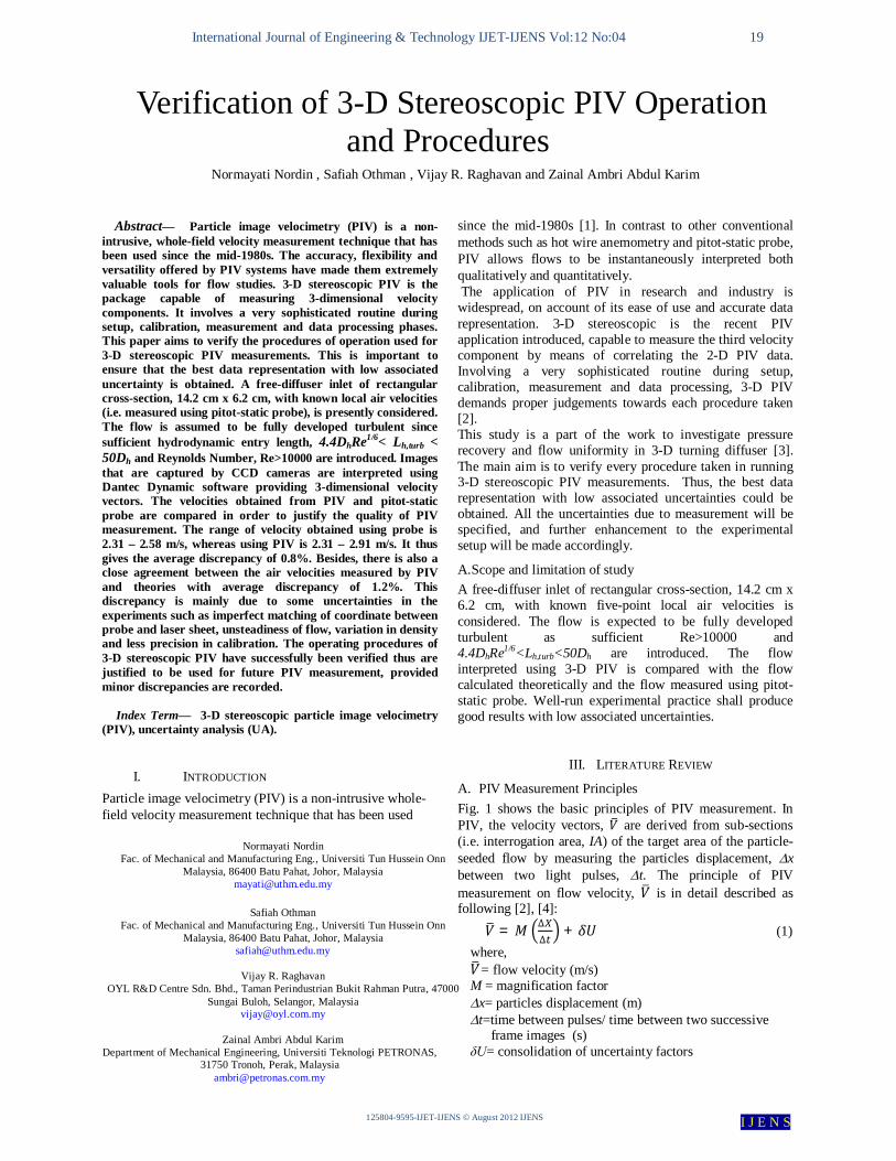
A. PIV Measurement Principles Fig. 1 shows the basic principles of PIV measurement. In PIV, the velocity vectors, 푉 are derived from sub-sections (i.e. interrogation area, IA) of the target area of the particle-seeded flow by measuring the particles displacement, x between two light pulses, t. The principle of PIV measurement on flow velocity, 푉 is in detail described as following [2], [4]: 푉 = 푀 ∆

∆+ 훿푈 (1)

where, 푉= flow velocity (m/s) M = magnification factor x= particles displacement (m) t=time between pulses/ time between two successive frame images (s) δU= consolidation of uncertainty factors

Verification of 3-D Stereoscopic PIV Operation and Procedures

Normayati Nordin , Safiah Othman , Vijay R. Raghavan and Zainal Ambri Abdul Karim



Raffel et al. [1] have defined magnification factor, M as the ratio of the distance between the image plane and lens, S’ to the distance between the lens and object plane, S. In the present work, the plane target is placed approximately at S = 10S’. In this study, the target area of the flow is illuminated with double pulses Neodym: YAG laser. The laser light sheet thickness for stereoscopic PIV application is

Fig. 1. PIV measurement principles [6] recommended to be approximately twice the size of the interrogation area (dIA) projected out in object space [5]. This factor 2 is necessary to compensate for the Gaussian distribution of the light intensity. The laser sheet thickness can be estimated as following: 퐿푎푠푒푟푠ℎ푒푒푡푡ℎ푖푐푘푛푒푠푠 = ( × × )

(2)

With modern charge coupled device (CCD) cameras (1000 x 1000 sensor elements and more), it is possible to capture more than 100 PIV recordings per minute [1]. High-speed recording on complementary metal-oxide semiconductor (CMOS) sensors even allows for acquisition in the kHz [1]. The cameras are able to capture each light pulse in separate image frames. Once a sequence of two light pulses is recorded, the interrogation areas from each image frame, I1 and I2, are cross-correlated with each other, pixel by pixel.

In contrast to hot wire or pitot-static probe techniques, PIV measures the flow indirectly by determining the particle velocity instead of the flow velocity. Therefore, fluid mechanical properties of the tracer particle have to be examined in order to avoid significant discrepancies between fluid and particle motion. In air flows, smoke or oil drops within the diameter range of 0.5 µm to 10 µm are often used as tracer particles [1], [6]. Basically, any particle that follows the flow satisfactorily and scatters enough light to be captured by the camera can be used. In this study, water- based smoke; Eurolite with an average diameter of 1±0.001 µm is used. Besides that, the tracer particles should be introduced in a way and at a location that ensures homogeneous distribution of the tracers. Since the existing turbulence in many test setups is not strong enough to mix the fluid and particles

sufficiently, the particles have to be supplied from a large number of openings [1]. The number of particles in the flow is of some importance in obtaining a good signal peak in cross correlation. As a rule of thumb, 10 to 25 particle images should be seen in each interrogation area [6]. The highest measureable velocity, V is constrained by particles travelling further than the size of the interrogation area, dIA within the time, t. The result is lost correlation between the two image frames and thus loss of velocity information. As a rule of thumb [6]:

. .∆ < 25% (3)

B. Uncertainty Measurement and Analysis No measurement is exact. When a quantity is measured,

the outcome depends on the measuring system, the measurement procedure, the skill of the operator, the environment and other effects. Even if the quantity were to be measured several times, in the same way, and in the same circumstances, a different measured value would in general be obtained each time, assuming that the measuring system has sufficient resolution to distinguish between the values.

3-D turning diffusers with area ratios of 2.0 and 4.0 were considered previously by Normayati et al. [3], where stereoscopic PIV was used to judge the flow within. The 3-D turning diffuser with an area ratio of 4.0 was found to be more favourable used, particularly when a low Reynolds number of 20 was applied. Nevertheless, the results obtained are still subject to certain doubt, as the verification and validation of the experimentation has never been performed.

The PIV measurement system consists of several sub-systems namely; (1) calibration, (2) flow visualization, (3) image detection and (4) data processing [2]. Each sub-system is often associated with uncertainties that on the whole can affect the quality of measurement. Therefore, the evaluation of PIV measurement basically needs to consider the coupling between the sub-systems.

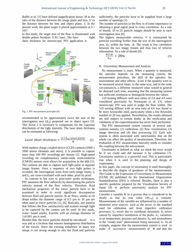
Uncertainty is defined as what we think the error would be if we could and did measure it by calibration [7]. Uncertainty analysis is a powerful tool. This is particularly true when it is used in the planning and design of experiments. In this paper, the concept of uncertainty is used thoroughly to describe the degree of goodness of the measurements. The Guide to the Expression of Uncertainty in Measurement (GUM) [8] published by the International Organization Standardisation (ISO) is referred. Besides, there is also a specific guideline prepared by the Visualisation Society of Japan [4] to perform uncertainty analysis for PIV measurement. Consider a variable W in a process that is considered to be steady so that its true value (Wtrue) is constant. Measurements of the variable are influenced by a number of elemental error sources- such as the errors in the standard used for calibration and from imperfect calibration processes, δ1; errors due to coordinate mismatch, δ2; errors caused by imperfect installation of the probe, δ3; variations in air temperature, pressure and density, δ4; and unsteadiness in the “steady state” phenomenon being measured, δ5. As an example, suppose that the measurement system is used to make N successive measurements of W and that the



measurements are influenced by these five significant error sources, as shown in Fig. 2. Each of the measurements has a different value since errors from some of the sources vary (i.e. random errors) during the period when measurements are taken, while some do not vary (i.e. systematic errors, formerly known as bias errors). Systematic error is assigned with the symbol, β whereas random error, ε. If the errors from source 1 and 2 do not vary and the errors from sources 3, 4 and 5 do vary,

Fig. 2. Measurement of variable W influenced by five error sources

WN can be written as;

WN= Wtrue + β + (ε )N (4)

where β = β1 + β2 (systematic/bias errors) (ε )N = (ε 3)N + (ε 4)N + (ε 5)N (random errors) Wtrue= true value (theoretical value) WN= measurement value (experimental value) N = number of experiment

Percentage of error or discrepancies is commonly determined by comparing the experimental and theoretical values. However, it quantifies nothing on which source of errors contribute more to the discrepancies. It is basically worth to specify some range (Wbest±uW) within which we think Wtrue falls. Generally, Wbest is taken to be equal to the average value of the N measurements, while (±uW) is the uncertainty interval that likely contains the magnitude of the combination of all the errors affecting the measured value W. Elemental uncertainty estimates for all elemental error sources are needed in order to associate an uncertainty with a measured W value. For example, u1 is an uncertainty that defines an interval (±u1) within which the value of β1 falls, while u3 is an uncertainty that defines an interval (±u3) within which the value of ε 3 falls. Using the concepts and procedures by ISO [8], a standard uncertainty, u is defined as an estimate of the standard deviation of the parent population from which a particular elemental error originates. Then uW is found from the combination of all of the elemental standard uncertainties as a root sum square value thus:

uW = (u1

2+ u22+ u3

2+ u42+ u5

2)1/2 (5)

For N measurements of W, the standard deviation, sW can be calculated as:

푠 = ∑ (푊 −푊)⁄

(6)

where the mean value of W is calculated from: 푊 = ∑ 푊 (7)

Basically, only the effects of random errors are included in sW, but not systematic errors. Thus:

sw = (u3

2 + u42 + u5

2)1/2 (8) and so Eq. (5) becomes: uW = (u1

2+ u22+ sw

2)1/2 (9)

This leaves the standard uncertainties for the systematic error sources, u1 and u2 to be estimated before the standard uncertainty uW can be determined. The systematic standard uncertainties are designated with symbol b, which is understood to be an estimate of the standard deviation of the distribution of the parent population from which a particular systematic error β originates. It can be estimated in a variety of ways such as via statistical approach, use of previous experience, manufacturer’s specifications, calibration data, pilot study, result from analytical model etc.

Standard uncertainty which is determined using statistical approach is categorized as a type A uncertainty evaluation, whereas using other than statistical approach is categorized as type B uncertainty evaluation [8]. Therefore, Eq. (9) would become, considering uncertainty b1 and SW determined via statistical approach, while b2 by means of the other approach.

uW = (b1,A

2+ b2,B2+ sw,A

2)1/2 (10)

C. Turbulence characteristics The flow in a round pipe that is introduced having

Reynolds Number of more than 4000 is practically characterized as turbulent [9]. However, this is not always the case as the flow transition depends upon the degree of disturbance of the flow by surface roughness, pipe vibrations, and fluctuations in the upstream flows [10]. Many of conduits that are used are not circular in cross-section. Although the details of the flow in such conduits depend on the exact cross-sectional shape, many round pipe results can be carried over, with slight modification, to flow in conduits of other shape. Practical, easy-to-use results can be obtained by introducing hydraulic diameter, Dh=4A/P. For turbulent flow such calculations are usually accurate to within about 15% [9]. The most convenient way to compare the experimental results from PIV with the CFD simulation predictions is at a steady state condition with fully developed flow at the entrance of the diffuser [11]. In order to generate such condition, several criteria should be taken into consideration [11]; (1) the pipe should be sufficiently long to ensure the flow is fully developed, Lh,turb/Dh= 4.4Re1/6 [9], Lh,turb/Dh= 1.359Re1/4 or Lh,turb ≈10Dh [10], Lh,turb ≈50 Dh [11]; (2) no flexible tube should be used as it creates disturbance in the system due to its movement [11]; (3) a precise blower is required to maintain flow at one set point [11]; (4) a precise control system should maintain the flow rate at a specific set point [11]; (5) systematic and same procedures should be applied towards each measurement taken [11].

Measurement system Wtrue

WN= Wtrue + (δ1)N + (δ2)N + (δ3)N + (δ4)N + (δ5)N

δ1

δ2 δ3

δ4 δ5



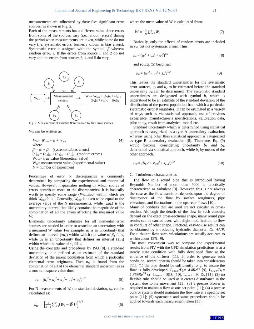
Fig. 3. The velocity profile, W(y) in fully developed flow becomes flatter or fuller in turbulent flow Because of the size of the equipment and the dimensions of the lab space, criterion (1) could be the best applied, by introducing the hydrodynamic length of 4.4DhRe1/6<Lh,turb<50Dh, i.e. 206 cm [9], [11]. Criterion (2) could not technically be met because, during the measurements, it was necessary to incline the test object to certain height that could suit the PIV setup. Due to the limitations of the experimental setup here criteria (3) and (4) could not be met. In general, it is actually difficult to achieve a perfect steady state fully developed condition [11]. Unlike laminar flow, the expressions for the velocity profile in a turbulent flow are based on both analysis and measurements, and thus they are semi-empirical in nature with constants determined from the experiment. As illustrated in Fig. 3, the velocity profile in fully developed turbulent flow is much fuller, with a sharp drop near the wall. Turbulent flow along a wall can be considered to consist of four regions, namely viscous sublayer, buffer layer, overlap layer and outer turbulent layer.

Each layer is characterised by the distance from the wall, 푟 = ∗, where u* is a friction velocity that can be

calculated using 푢∗ = 휏 휌⁄ and r=b/2 - y. Wall shear stress, 휏 can be determined using 휏 = 푓휌푊 , with friction factor, f that depends on Re and relative roughness, ε/Dh and can be found from Moody chart. As the measurement points of P4 and P5 are located at r+>30, they are both within the outer turbulent layer. Therefore, the one-seventh power-law velocity profile can be applied as following:

= 1 −⁄

(11)

Fig. 5. Measurement points; P1, P2, P3, P4 and P5

where, WPn = local velocity (m/s) Umax= velocity at the centre point, i.e. WP2 (m/s) y = measurement point from the centre (m) R = Dh/2 (m)

IV. METHODOLOGY

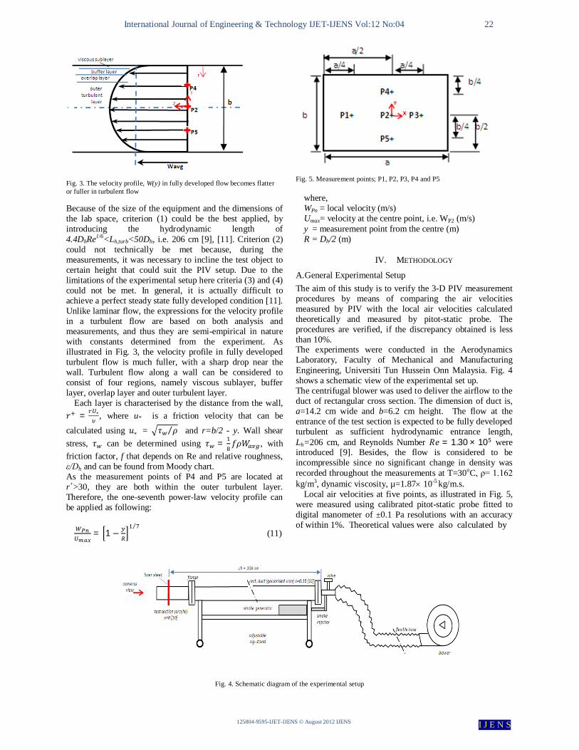
A. General Experimental Setup The aim of this study is to verify the 3-D PIV measurement procedures by means of comparing the air velocities measured by PIV with the local air velocities calculated theoretically and measured by pitot-static probe. The procedures are verified, if the discrepancy obtained is less than 10%. The experiments were conducted in the Aerodynamics Laboratory, Faculty of Mechanical and Manufacturing Engineering, Universiti Tun Hussein Onn Malaysia. Fig. 4 shows a schematic view of the experimental set up. The centrifugal blower was used to deliver the airflow to the duct of rectangular cross section. The dimension of duct is, a=14.2 cm wide and b=6.2 cm height. The flow at the entrance of the test section is expected to be fully developed turbulent as sufficient hydrodynamic entrance length, Lh=206 cm, and Reynolds Number 푅푒 = 1.30 × 10 were introduced [9]. Besides, the flow is considered to be incompressible since no significant change in density was recorded throughout the measurements at T=30oC, ρ= 1.162 kg/m3, dynamic viscosity, µ=1.87 10-5 kg/m.s.

Local air velocities at five points, as illustrated in Fig. 5, were measured using calibrated pitot-static probe fitted to digital manometer of ±0.1 Pa resolutions with an accuracy of within 1%. Theoretical values were also calculated by

Fig. 4. Schematic diagram of the experimental setup



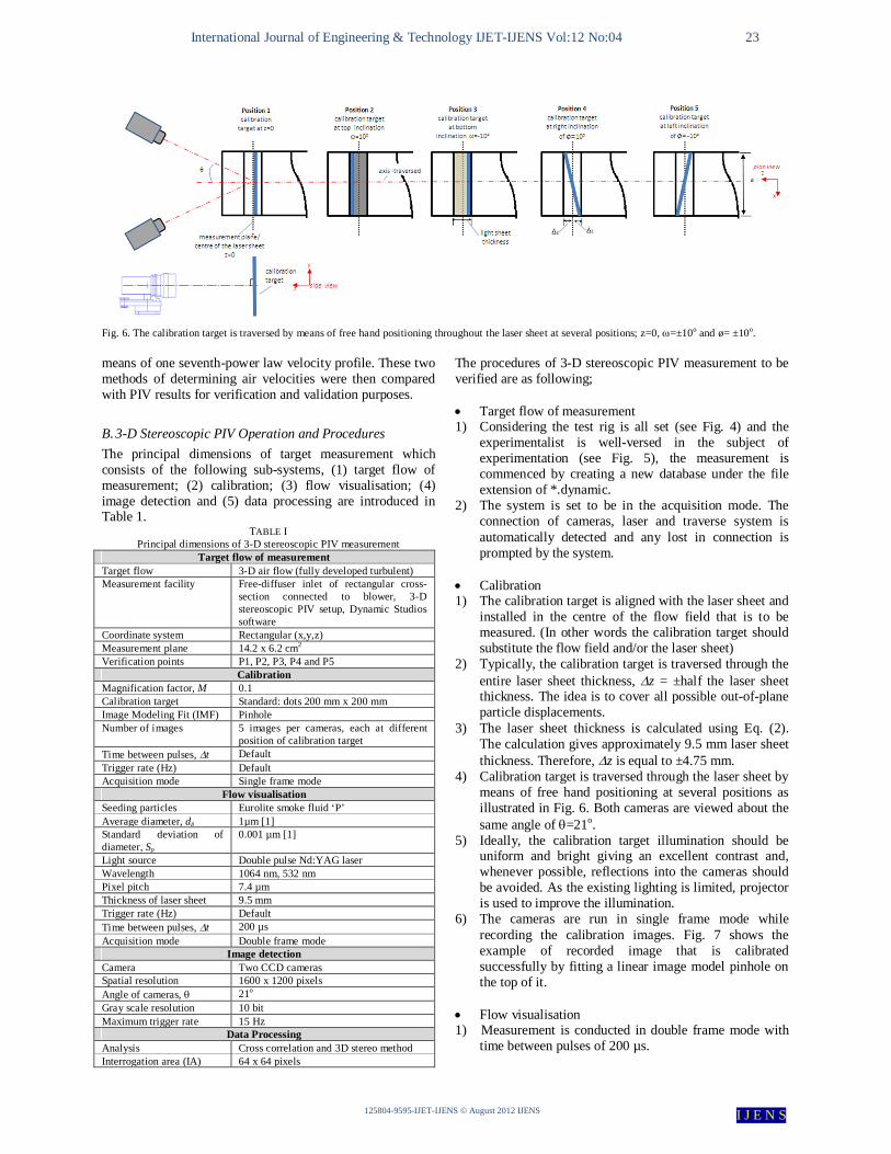
Fig. 6. The calibration target is traversed by means of free hand positioning throughout the laser sheet at several positions; z=0, =±10o and ø= ±10o. means of one seventh-power law velocity profile. These two methods of determining air velocities were then compared with PIV results for verification and validation purposes.

B. 3-D Stereoscopic PIV Operation and Procedures The principal dimensions of target measurement which consists of the following sub-systems, (1) target flow of measurement; (2) calibration; (3) flow visualisation; (4) image detection and (5) data processing are introduced in Table 1.

TABLE I Principal dimensions of 3-D stereoscopic PIV measurement

Target flow of measurement Target flow 3-D air flow (fully developed turbulent) Measurement facility Free-diffuser inlet of rectangular cross-

section connected to blower, 3-D stereoscopic PIV setup, Dynamic Studios software

Coordinate system Rectangular (x,y,z) Measurement plane 14.2 x 6.2 cm2 Verification points P1, P2, P3, P4 and P5

Calibration Magnification factor, M 0.1 Calibration target Standard: dots 200 mm x 200 mm Image Modeling Fit (IMF) Pinhole Number of images 5 images per cameras, each at different

position of calibration target Time between pulses, t Default Trigger rate (Hz) Default Acquisition mode Single frame mode

Flow visualisation Seeding particles Eurolite smoke fluid ‘P’ Average diameter, dp 1µm [1] Standard deviation of diameter, Sp

0.001 µm [1]

Light source Double pulse Nd:YAG laser Wavelength 1064 nm, 532 nm Pixel pitch 7.4 µm Thickness of laser sheet 9.5 mm Trigger rate (Hz) Default Time between pulses, t 200 µs Acquisition mode Double frame mode

Image detection Camera Two CCD cameras Spatial resolution 1600 x 1200 pixels Angle of cameras, 21o Gray scale resolution 10 bit Maximum trigger rate 15 Hz

Data Processing Analysis Cross correlation and 3D stereo method Interrogation area (IA) 64 x 64 pixels

The procedures of 3-D stereoscopic PIV measurement to be verified are as following;

Target flow of measurement 1) Considering the test rig is all set (see Fig. 4) and the

experimentalist is well-versed in the subject of experimentation (see Fig. 5), the measurement is commenced by creating a new database under the file extension of *.dynamic.

2) The system is set to be in the acquisition mode. The connection of cameras, laser and traverse system is automatically detected and any lost in connection is prompted by the system.

Calibration 1) The calibration target is aligned with the laser sheet and

installed in the centre of the flow field that is to be measured. (In other words the calibration target should substitute the flow field and/or the laser sheet)

2) Typically, the calibration target is traversed through the entire laser sheet thickness, z = ±half the laser sheet thickness. The idea is to cover all possible out-of-plane particle displacements.

3) The laser sheet thickness is calculated using Eq. (2). The calculation gives approximately 9.5 mm laser sheet thickness. Therefore, z is equal to ±4.75 mm.

4) Calibration target is traversed through the laser sheet by means of free hand positioning at several positions as illustrated in Fig. 6. Both cameras are viewed about the same angle of =21o.

5) Ideally, the calibration target illumination should be uniform and bright giving an excellent contrast and, whenever possible, reflections into the cameras should be avoided. As the existing lighting is limited, projector is used to improve the illumination.

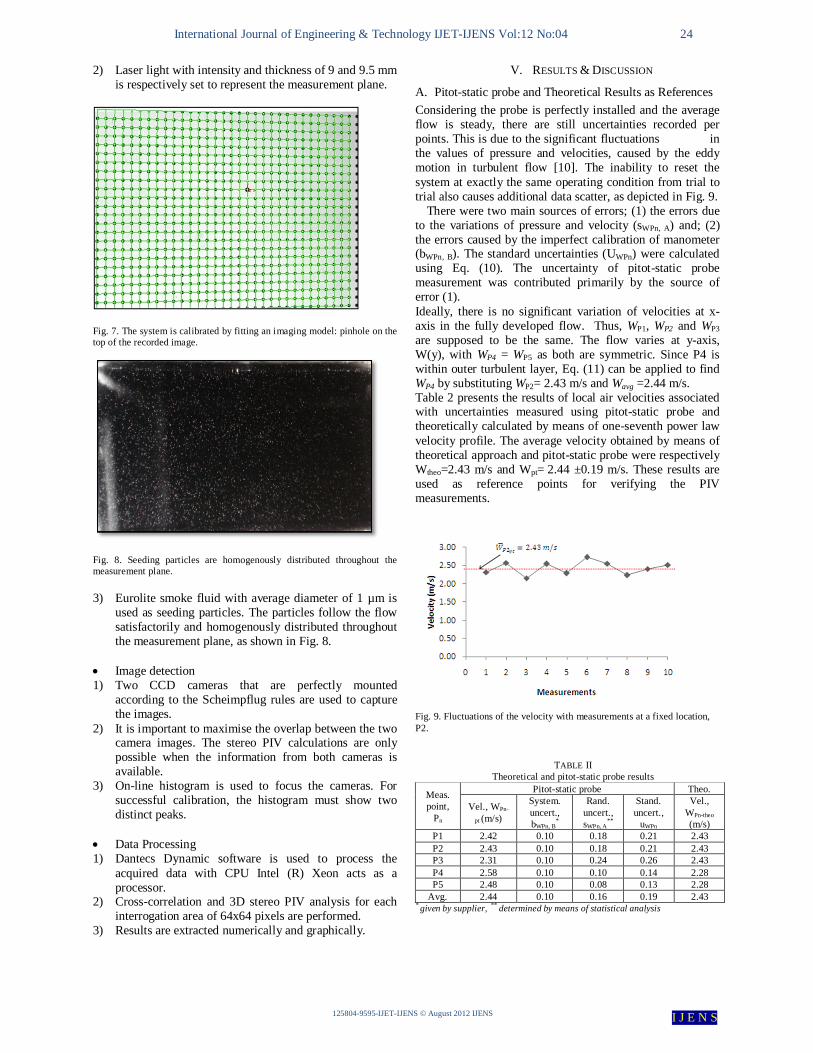
6) The cameras are run in single frame mode while recording the calibration images. Fig. 7 shows the example of recorded image that is calibrated successfully by fitting a linear image model pinhole on the top of it.

Flow visualisation 1) Measurement is conducted in double frame mode with

time between pulses of 200 µs.



2) Laser light with intensity and thickness of 9 and 9.5 mm is respectively set to represent the measurement plane.

Fig. 7. The system is calibrated by fitting an imaging model: pinhole on the top of the recorded image.

Fig. 8. Seeding particles are homogenously distributed throughout the measurement plane. 3) Eurolite smoke fluid with average diameter of 1 µm is

used as seeding particles. The particles follow the flow satisfactorily and homogenously distributed throughout the measurement plane, as shown in Fig. 8.

Image detection 1) Two CCD cameras that are perfectly mounted

according to the Scheimpflug rules are used to capture the images.

2) It is important to maximise the overlap between the two camera images. The stereo PIV calculations are only possible when the information from both cameras is available.

3) On-line histogram is used to focus the cameras. For successful calibration, the histogram must show two distinct peaks.

Data Processing 1) Dantecs Dynamic software is used to process the

acquired data with CPU Intel (R) Xeon acts as a processor.

2) Cross-correlation and 3D stereo PIV analysis for each interrogation area of 64x64 pixels are performed.

3) Results are extracted numerically and graphically.

V. RESULTS & DISCUSSION

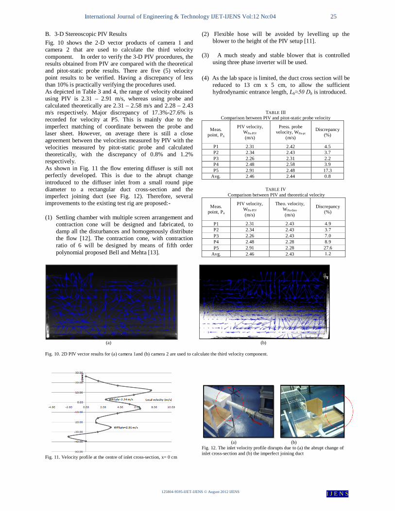
A. Pitot-static probe and Theoretical Results as References Considering the probe is perfectly installed and the average flow is steady, there are still uncertainties recorded per points. This is due to the significant fluctuations in the values of pressure and velocities, caused by the eddy motion in turbulent flow [10]. The inability to reset the system at exactly the same operating condition from trial to trial also causes additional data scatter, as depicted in Fig. 9.

There were two main sources of errors; (1) the errors due to the variations of pressure and velocity (sWPn, A) and; (2) the errors caused by the imperfect calibration of manometer (bWPn, B). The standard uncertainties (UWPn) were calculated using Eq. (10). The uncertainty of pitot-static probe measurement was contributed primarily by the source of error (1). Ideally, there is no significant variation of velocities at x-axis in the fully developed flow. Thus, WP1, WP2 and WP3 are supposed to be the same. The flow varies at y-axis, W(y), with WP4 = WP5 as both are symmetric. Since P4 is within outer turbulent layer, Eq. (11) can be applied to find WP4 by substituting WP2= 2.43 m/s and Wavg =2.44 m/s. Table 2 presents the results of local air velocities associated with uncertainties measured using pitot-static probe and theoretically calculated by means of one-seventh power law velocity profile. The average velocity obtained by means of theoretical approach and pitot-static probe were respectively Wtheo=2.43 m/s and Wpt= 2.44 ±0.19 m/s. These results are used as reference points for verifying the PIV measurements.

Fig. 9. Fluctuations of the velocity with measurements at a fixed location, P2.

TABLE II Theoretical and pitot-static probe results

Meas. point,

Pn

Pitot-static probe Theo.

Vel., WPn-

pt (m/s)

System. uncert., bWPn, B

*

Rand. uncert., sWPn, A

**

Stand. uncert.,

uWPn

Vel., WPn-theo (m/s)

P1 2.42 0.10 0.18 0.21 2.43 P2 2.43 0.10 0.18 0.21 2.43 P3 2.31 0.10 0.24 0.26 2.43 P4 2.58 0.10 0.10 0.14 2.28 P5 2.48 0.10 0.08 0.13 2.28

Avg. 2.44 0.10 0.16 0.19 2.43 * given by supplier, ** determined by means of statistical analysis



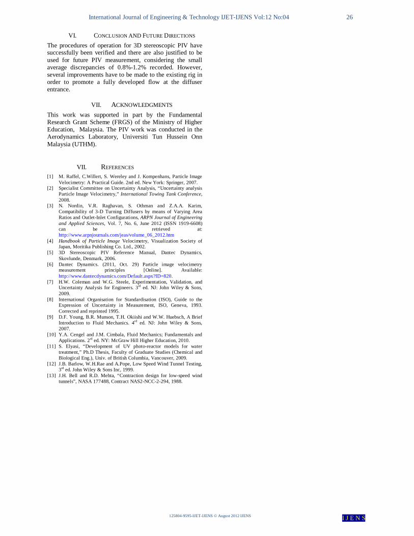
B. 3-D Stereoscopic PIV Results Fig. 10 shows the 2-D vector products of camera 1 and camera 2 that are used to calculate the third velocity component. In order to verify the 3-D PIV procedures, the results obtained from PIV are compared with the theoretical and pitot-static probe results. There are five (5) velocity point results to be verified. Having a discrepancy of less than 10% is practically verifying the procedures used. As depicted in Table 3 and 4, the range of velocity obtained using PIV is 2.31 – 2.91 m/s, whereas using probe and calculated theoretically are 2.31 – 2.58 m/s and 2.28 – 2.43 m/s respectively. Major discrepancy of 17.3%-27.6% is recorded for velocity at P5. This is mainly due to the imperfect matching of coordinate between the probe and laser sheet. However, on average there is still a close agreement between the velocities measured by PIV with the velocities measured by pitot-static probe and calculated theoretically, with the discrepancy of 0.8% and 1.2% respectively. As shown in Fig. 11 the flow entering diffuser is still not perfectly developed. This is due to the abrupt change introduced to the diffuser inlet from a small round pipe diameter to a rectangular duct cross-section and the imperfect joining duct (see Fig. 12). Therefore, several improvements to the existing test rig are proposed:-

(1) Settling chamber with multiple screen arrangement and contraction cone will be designed and fabricated, to damp all the disturbances and homogenously distribute the flow [12]. The contraction cone, with contraction ratio of 6 will be designed by means of fifth order polynomial proposed Bell and Mehta [13].

(2) Flexible hose will be avoided by levelling up the blower to the height of the PIV setup [11].

(3) A much steady and stable blower that is controlled using three phase inverter will be used.

(4) As the lab space is limited, the duct cross section will be

reduced to 13 cm x 5 cm, to allow the sufficient hydrodynamic entrance length, Lh≈50 Dh is introduced.

TABLE III Comparison between PIV and pitot-static probe velocity

Meas. point, Pn

PIV velocity, WPn-PIV (m/s)

Press. probe velocity, WPn-pt

(m/s)

Discrepancy (%)

P1 2.31 2.42 4.5 P2 2.34 2.43 3.7 P3 2.26 2.31 2.2 P4 2.48 2.58 3.9 P5 2.91 2.48 17.3

Avg. 2.46 2.44 0.8

TABLE IV Comparison between PIV and theoretical velocity

Meas. point, Pn

PIV velocity, WPn-PIV

(m/s)

Theo. velocity, WPn-theo

(m/s)

Discrepancy (%)

P1 2.31 2.43 4.9 P2 2.34 2.43 3.7 P3 2.26 2.43 7.0 P4 2.48 2.28 8.9 P5 2.91 2.28 27.6

Avg. 2.46 2.43 1.2

(a) (b) Fig. 10. 2D PIV vector results for (a) camera 1and (b) camera 2 are used to calculate the third velocity component.

Fig. 11. Velocity profile at the centre of inlet cross-section, x= 0 cm

(a) (b)

Fig. 12. The inlet velocity profile disrupts due to (a) the abrupt change of inlet cross-section and (b) the imperfect joining duct



VI. CONCLUSION AND FUTURE DIRECTIONS The procedures of operation for 3D stereoscopic PIV have successfully been verified and there are also justified to be used for future PIV measurement, considering the small average discrepancies of 0.8%-1.2% recorded. However, several improvements have to be made to the existing rig in order to promote a fully developed flow at the diffuser entrance.

VII. ACKNOWLEDGMENTS This work was supported in part by the Fundamental Research Grant Scheme (FRGS) of the Ministry of Higher Education, Malaysia. The PIV work was conducted in the Aerodynamics Laboratory, Universiti Tun Hussein Onn Malaysia (UTHM).

VII. REFERENCES [1] M. Raffel, C.Willert, S. Wereley and J. Kompenhans, Particle Image

Velocimetry: A Practical Guide. 2nd ed. New York: Springer, 2007. [2] Specialist Committee on Uncertainty Analysis, “Uncertainty analysis

Particle Image Velocimetry,” International Towing Tank Conference, 2008.

[3] N. Nordin, V.R. Raghavan, S. Othman and Z.A.A. Karim, Compatibility of 3-D Turning Diffusers by means of Varying Area Ratios and Outlet-Inlet Configurations, ARPN Journal of Engineering and Applied Sciences, Vol. 7, No. 6, June 2012 (ISSN 1919-6608) can be retrieved at: http://www.arpnjournals.com/jeas/volume_06_2012.htm

[4] Handbook of Particle Image Velocimetry, Visualization Society of Japan, Moritika Publishing Co. Ltd., 2002.

[5] 3D Stereoscopic PIV Reference Manual, Dantec Dynamics, Skovlunde, Denmark, 2006.

[6] Dantec Dynamics. (2011, Oct. 29) Particle image velocimetry measurement principles [Online]. Available: http://www.dantecdynamics.com/Default.aspx?ID=820.

[7] H.W. Coleman and W.G. Steele, Experimentation, Validation, and Uncertainty Analysis for Engineers. 3rd ed. NJ: John Wiley & Sons, 2009.

[8] International Organisation for Standardisation (ISO), Guide to the Expression of Uncertainty in Measurement, ISO, Geneva, 1993. Corrected and reprinted 1995.

[9] D.F. Young, B.R. Munson, T.H. Okiishi and W.W. Huebsch, A Brief Introduction to Fluid Mechanics. 4rd ed. NJ: John Wiley & Sons, 2007.

[10] Y.A. Cengel and J.M. Cimbala, Fluid Mechanics; Fundamentals and Applications. 2rd ed. NY: McGraw Hill Higher Education, 2010.

[11] S. Elyasi, “Development of UV photo-reactor models for water treatment,” Ph.D Thesis, Faculty of Graduate Studies (Chemical and Biological Eng.), Univ. of British Columbia, Vancouver, 2009.

[12] J.B. Barlow, W.H.Rae and A.Pope, Low Speed Wind Tunnel Testing, 3rd ed. John Wiley & Sons Inc, 1999.

[13] J.H. Bell and R.D. Mehta, “Contraction design for low-speed wind tunnels”, NASA 177488, Contract NAS2-NCC-2-294, 1988.

Verification of 3-D Stereoscopic PIV Operation and … · 2012-10-21 · 3-D stereoscopic PIV is...

Documents

Transcript of Verification of 3-D Stereoscopic PIV Operation and … · 2012-10-21 · 3-D stereoscopic PIV is...