Anecdotes from the history of mathematics ways of selling mathemati
Cop
yrig
ht ©
201
6 U
nive
rsity
of C
ambr
idge
. Not
to b
e qu
oted
or
repr
oduc
ed w
ithou
t per
mis
sion
.
Prepared for submission to JHEP
Vector Calculus IA
B. C. Allanacha J.M. Evansa
aDepartment of Applied Mathematics and Theoretical Physics, Centre for Mathemati-
cal Sciences, University of Cambridge, Wilberforce Road, Cambridge CB3 0WA, United
Kingdom
E-mail: [email protected]
Abstract: These are lecture notes for the Cambridge mathematics tripos Part IA
Vector Calculus course. There are four examples sheets for this course. These notes
are pretty much complete.
Books See the schedules for a list, but particularly:
• “Mathematical Methods for Physics and Engineering”, CUP 2002 by Riley,
Hobson and Bence £28.
• “Vector Analysis and Cartesian Tensors”, Bourne and Kendall 1999 by Nelson
Thomas £30.
Future lecturers: please feel free to use/modify this resource. If you do though, please
append your name to the current author list.
Cop
yrig
ht ©
201
6 U
nive
rsity
of C
ambr
idge
. Not
to b
e qu
oted
or
repr
oduc
ed w
ithou
t per
mis
sion
.
Contents
1 Derivatives and Coordinates 1
1.1 Differentiation Using Vector Notation 1
1.1.1 Vector function of a scalar 1
1.1.2 Scalar function of position; gradient and directional derivatives 2
1.1.3 The chain rule: a particular case 3
1.2 Differentiation Using Coordinate Notation 3
1.2.1 Differentiable functions ℜn → ℜm 3
1.2.2 The chain rule - general version 3
1.2.3 Inverse functions 4
1.3 Coordinate Systems 5
2 Curves and Line Integrals 6
2.1 Parameterised Curves, Tangents and Arc Length 6
2.2 Line Integrals of Vector Fields 8
2.2.1 Definitions and Examples 8
2.2.2 Comments 10
2.3 Sums of Curves and Integrals 10
2.4 Gradients and Exact Differentials 12
2.4.1 Line Integrals and Gradients 12
2.4.2 Differentials 13
2.5 Work and Potential Energy 13
3 Integration in ℜ2 and ℜ3 14
3.1 Integrals over subsets of ℜ2 14
3.1.1 Definition as the limit of a sum 14
3.1.2 Evaluation as multiple integrals 15
3.1.3 Comments 16
3.2 Change of Variables for an Integral in ℜ2 17
3.3 Generalisation to ℜ3 19
3.3.1 Definitions 19
3.3.2 Change of Variables in ℜ3 20
3.3.3 Examples 21
3.4 Further Generalisations and Comments 22
3.4.1 Integration in ℜn 22
3.4.2 Change of variables for the case n = 1 23
3.4.3 Vector valued integrals 23
– i –

Cop
yrig
ht ©
201
6 U
nive
rsity
of C
ambr
idge
. Not
to b
e qu
oted
or
repr
oduc
ed w
ithou
t per
mis
sion
.
4 Surfaces and Surface Integrals 24
4.1 Surfaces and Normals 24
4.2 Parameterised Surfaces and Area 26
4.3 Surface Integrals of Vector Fields 27
4.4 Comparing Line, Surface and Volume Integrals 30
4.4.1 Line and surface integrals and orientations 30
4.4.2 Change of variables in ℜ2 and ℜ3 revisited 30
5 Geometry of Curves and Surfaces 31
5.1 Curves, Curvature and Normals 31
5.2 Surfaces and Intrinsic Geometry (non-examinable) 32
6 Grad, Div and Curl 33
6.1 Definitions and Notation 33
6.2 Leibniz Properties 35
6.3 Second Order Derivatives 36
7 Integral Theorems 36
7.1 Statements and Examples 36
7.1.1 Green’s theorem (in the plane) 36
7.1.2 Stokes’ theorem 38
7.1.3 Divergence, or Gauss’ theorem 40
7.2 Relating and Proving the Integral Theorems 41
7.2.1 Proving Green’s theorem from Stokes’ theorem or the 2d di-
vergence theorem 41
7.2.2 Proving Green’s theorem by Proving the 2d Divergence Theo-
rem 42
7.2.3 Green’s theorem ⇒ Stokes’ theorem 45
7.2.4 Proving the divergence (or Gauss’) theorem in 3d: outline 46
8 Some Applications of Integral Theorems 47
8.1 Integral Expressions of Div and Curl 47
8.2 Conservative and Irrotational Fields, and Scalar Potentials 48
8.3 Conservation Laws 50
9 Othorgonal Curvilinear Coordinates 51
9.1 Line, Area and Volume Elements 51
9.2 Grad, Div and Curl 52
10 Gauss’ Law and Poisson’s Equation 55
10.1 Laws of Gravitation 55
10.2 Laws of Electrostatics 57
– ii –
Cop
yrig
ht ©
201
6 U
nive
rsity
of C
ambr
idge
. Not
to b
e qu
oted
or
repr
oduc
ed w
ithou
t per
mis
sion
.
10.3 Poisson’s Equation and Laplace’s Equation 58
11 General Results for Laplace’s and Poisson’s Equations 61
11.1 Uniqueness Theorems 61
11.1.1 Statement and proof 61
11.1.2 Comments 62
11.2 Laplace’s Equation and Harmonic Functions 63
11.2.1 The Mean Value Property 63
11.2.2 The Maximum (or Minimum) Principle 64
11.3 Integral Solution of Poisson’s Equation 64
11.3.1 Statement and informal derivation 64
11.3.2 Point sources and δ−functions (non-examinable) 65
12 Maxwell’s Equations 66
12.1 Laws of Electromagnetism 66
12.2 Static Charges and Steady Currents 67
12.3 Electromagnetic Waves 67
13 Tensors and Tensor Fields 68
13.1 Definitions and Examples 68
13.1.1 Tensor transformation rule 68
13.1.2 Basic examples 68
13.1.3 Rank 2 tensors and matrices 69
13.2 Tensor Algebra 69
13.2.1 Addition and scalar multiplication 69
13.2.2 Tensor products 69
13.2.3 Contractions 69
13.2.4 Symmetric and antisymmetric tensors 70
13.3 Tensors, Multi-linear Maps and the Quotient Rule 70
13.3.1 Tensors as multi-linear maps 70
13.3.2 The quotient rule 71
13.4 Tensor Calculus 71
13.4.1 Tensor fields and derivatives 71
13.4.2 Integrals and the tensor divergence theorem 72
14 Tensors of Rank 2 73
14.1 Decomposition of a Second Rank Tensor 73
14.2 The Inertia Tensor 73
14.3 Diagonalisation of a Symmetric Second Rank Tensor 74
– iii –
Cop
yrig
ht ©
201
6 U
nive
rsity
of C
ambr
idge
. Not
to b
e qu
oted
or
repr
oduc
ed w
ithou
t per
mis
sion
.
15 Invariant and Isotropic Tensors 75
15.1 Definitions and Classification Results 75
15.2 Application to Invariant Integrals 75
15.3 A Sketch of a Proof of Classification Results for Rank n ≤ 3 76
1 Derivatives and Coordinates
1.1 Differentiation Using Vector Notation
1.1.1 Vector function of a scalar
A vector function F (u) is ‘differentiable’ at u if
δF = F (u+ δu)− F (u) = F ′(u)δu+ o(δu) as δu→ 0,
and the derivative is the vector
F ′(u) =dF
du= limδu→0
1
δu[F (u+ δu)− F (u)] .
Limits of vectors are defined using the norm(length) so v → c iff |v− c| → 0 and
a(h) = b(h) + no(h) iff |a(h)− b(h)| = o(h), for n some unit vector.
Leibniz identities hold for appropriate products of scalar functions f(u) and vec-
tors F (u), G(u):
(fF )′ = f ′F + fF ′, (F ·G)′ = F ′ ·G+ F ·G′,
(F ∧G)′ = F ′ ∧G+ F ∧G′.
Vectors can be differentiated component by component:
F (u) = Fi(u)ei ⇒ F ′(u) = F ′i (u)ei
provided the basis {ei} is independent of u (note the implicit summation convention
over repeated indices).
The definition of the derivative can be abbreviated using differential notation
dF = F ′(u) du in which o−terms are suppressed, compared to the relation above
with small but finite changes.
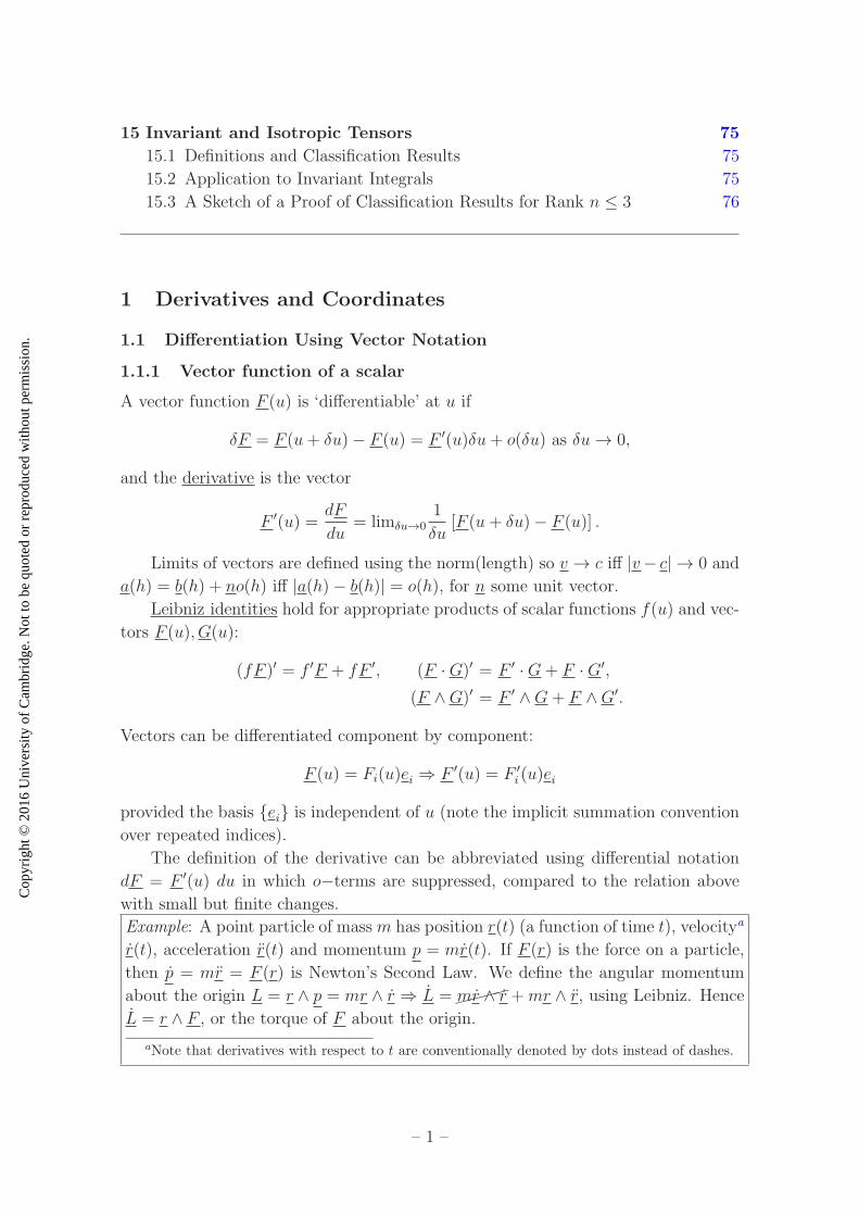
Example: A point particle of massm has position r(t) (a function of time t), velocitya
r(t), acceleration r(t) and momentum p = mr(t). If F (r) is the force on a particle,
then p = mr = F (r) is Newton’s Second Law. We define the angular momentum
about the origin L = r ∧ p = mr ∧ r ⇒ L =����mr ∧ r +mr ∧ r, using Leibniz. Hence
L = r ∧ F , or the torque of F about the origin.
aNote that derivatives with respect to t are conventionally denoted by dots instead of dashes.
– 1 –

Cop
yrig
ht ©
201
6 U
nive
rsity
of C
ambr
idge
. Not
to b
e qu
oted
or
repr
oduc
ed w
ithou
t per
mis
sion
.
1.1.2 Scalar function of position; gradient and directional derivatives
A scalar function f(r) is differentiable at r if
δf(r + δr)− f(r) = (∇f) · δr + o(|δr|) as |δr| → 0.
∇f is a vector, the gradient of f at r. The definition says that δf depends linearly
on δr, up to smaller o−terms.
Taking δr = hn with n a unit vector,
δf = f(r + hn)− f(r) = (∇f) · (hn) + o(h)
⇒ n · ∇f = limh→01
h[f(r + hn)− f(r)] ,
the directional derivative of f along n. Thus, the gradient contains information about
how f changes as we move away from r to first order in the displacement.
Let r = xiei with {ei} orthonormal. Setting n = ei for fixed i gives
ei · ∇f = limh→01
h[f(r + hei)− f(r)] =
∂f
∂xi.
Hence the gradient in Cartesian coordinates is
∇f =∂f
∂xiei. (1.1)
With this choice of basis and coordinates, the definition of differentiability becomes
δf =∂f
∂xiδxi + o(δx)
as δx =√δxiδxi → 0. In differential notation, we suppress o−terms:
df = ∇f · dr = ∂f
∂xidxi.
Example: f(x, y, z) = x+ exy sin z at (x, y, z) = (0, 1, 0).
∇f =
(∂f
∂x,∂f
∂y,∂f
∂z
)
= (1 + yexy sin z, xexy sin z, exy cos z) ,
thus ∇f = (1, 0, 1) at (x, y, z) = (0, 1, 0). The rate of change of f along direction
n is given by the directional derivative n · ∇f . So f increases most rapidly for n =
+ 1√2(1, 0, 1) and decreases most rapidly for n = − 1√
2(1, 0, 1) at a rate n ·∇f = ±
√2.
To first order, there is no change in f if n ⊥ (1, 0, 1).
– 2 –
Cop
yrig
ht ©
201
6 U
nive
rsity
of C
ambr
idge
. Not
to b
e qu
oted
or
repr
oduc
ed w
ithou
t per
mis
sion
.
1.1.3 The chain rule: a particular case
Consider a composition of differentiable functions f(r(u)). A change δu produces a
change δr = r′δu+ o(δu) and
δf = ∇f · δr + o(|δr|) = ∇f · r′(u)δu+ o(δu).
This shows that f is differentiable as a function of u and
df
du= ∇f · dr
du,
a chain rule. In Cartesian coordinates (setting r = xiei),dfdu
= ∂f∂xi
dxidu
.
1.2 Differentiation Using Coordinate Notation
1.2.1 Differentiable functions ℜn → ℜm
The functions F (u) and f(r) discussed in sections 1.1.1,1.1.2 are maps ℜ → ℜ3 and
ℜ3 → ℜ while a vector field F (r) is a function ℜ3 → ℜ3.
In general, f : ℜn{xi} → ℜm{yr} is equivalent to a set of functions yr = Fr(x1, . . . , xn) =
Fr(xi) where r = 1, . . . ,m and i = 1, . . . , n. The function f is differentiable if
δyr =M(f)riδxi + o(δx) as δx =√δxiδxi → 0, with derivative M(f)ri =
∂yr∂xi
= ∂Fr
∂xj,
a m × n matrix of partial derivatives. For example, for ℜ3 → ℜ, we get a 1 × 3
matrix, or vector, gradient i.e. (∂f∂x, ∂f∂y, ∂f∂z).
A convenient abbreviation of the definition: replace small changes by differentials
and drop the o−terms, which are understood.
dyr =M(f)ridxi =∂yr∂xi
dxi.
A function is smooth if it can be differentiated any number of times, i.e. if all partial
derivatives exist, for example ∂2Fr
∂xi∂xj, ∂3Fr
∂xi∂xj∂xketc, and these are totally symmetric
in i, j, k, . . . For example, ∂2Fr
∂xi∂xj= ∂2Fr
∂xj∂xi. The functions that we will consider here
will be smooth except for where things obviously go wrong, eg f(x) = 1/x is smooth
except at x = 0.
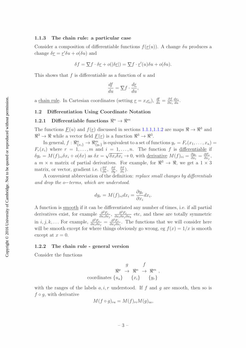
1.2.2 The chain rule - general version
Consider the functions
g f
ℜp → ℜn → ℜmcoordinates {ua} {xi} {yr}
,
with the ranges of the labels a, i, r understood. If f and g are smooth, then so is
f ◦ g, with derivative
M(f ◦ g)ra =M(f)riM(g)ia,
– 3 –

Cop
yrig
ht ©
201
6 U
nive
rsity
of C
ambr
idge
. Not
to b
e qu
oted
or
repr
oduc
ed w
ithou
t per
mis
sion
.
or matrix multiplication
∂yr∂ua
m× p =∂yr∂xi
∂xi∂ua
m× n n× p matrix type
Thus, if we compare the functions, we also compose the derivatives (matrices) as
linear maps.
dyr =M(f)ridxidxi =M(g)iadua
}
combine and compare with dyr =M(f ◦ g)radua.
In operator form, ∂∂ua
= ∂xi∂ua
∂∂xi
, which holds when acting on any function which
depends on ua through xi.
For example, y = f(xi(u)) ℜ → ℜ3 → ℜdydu
= ∂y∂xi
dxidu
1× 1 1× 3 3× 1.
Compare with section 1.1.3.
1.2.3 Inverse functions
With the notation of the last section, takem = n = p and let f, g be inverse functions,
both smooth, with yr = ur:g
→ℜn ℜn←f
{ua} {xi}Both f ◦ g and g ◦ f are identity functions on ℜn. M(f ◦ g)ia and M(g ◦ f) are
n × n identity matrices. M(f)ai and M(g)ia are inverse matrices of each other.
Equivalently, ∂ub∂ua
= ∂ub∂xi
∂xi∂ua
= δab;∂xj∂xi
=∂xj∂ua
∂ua∂xi
= δij.
For n = 1, we get the familiar result dudx
= 1dx/du
.
For n > 1, we must invert matrices to relate ∂xi∂ua
and ∂ua∂xi
.
For example: for n = 2, we write u1 = ρ, u2 = ϕ and let x1 = ρ cosϕ, x2 = ρ sinϕ.
M(g) =
(∂x1∂ρ
∂x1∂ϕ
∂x2∂ρ
∂x2∂ϕ
)
=
(cosϕ −ρ sinϕsinϕ ρ cosϕ
)
.
The relations can be inverted i.e. ρ =√
x21 + x22 and ϕ = tan−1(x2/x1) (except that
ϕ is not defined at ρ = 0 and it is defined up to a multiple of 2π for ρ 6= 0). Then,
we can compute directly
M(f) =
(∂ρ∂x1
∂ρ∂x2
∂ϕ∂x1
∂ϕ∂x2
)
=M(g)−1 =
(
cosϕ sinϕ
−1ρsinϕ 1
ρcosϕ
)
(ρ 6= 0).
– 4 –

Cop
yrig
ht ©
201
6 U
nive
rsity
of C
ambr
idge
. Not
to b
e qu
oted
or
repr
oduc
ed w
ithou
t per
mis
sion
.
��
��������
����������������������������
����������
��������
��������
������������
������������
��
����
��
����
ρ
φ
x
x
e
e
1 1
2
2
eφ
eρ
Figure 1. Plane polar coordinates. ρ > 0 and 0 ≤ ϕ < 2π for uniqueness.
In general, for invertible smooth maps, as above, detM(g) = det(∂xi∂ua
)
, detM(f) =
det(∂ua∂xi
)
are called the Jacobians. They are non-zero, with
det
(∂xi∂ua
)
det
(∂ua∂xi
)
= 1, (no summation convention).
1.3 Coordinate Systems
Now, we apply the results of the last section to changes of coordinates on Euclidean
space. We can always choose to use Cartesian coordinates, but other choices are
often more useful. In general, the coordinates {ua} on Euclidean space (or some
subset of it) can be invertible functions of some Cartesian coordinates {xi} such that
ua({xi}) and xi({ua}) are smooth.
In 2 dimensions, we define plane polar coordinates ρ, ϕ by
x1 = ρ cosϕ, x2 = ρ sinϕ,
as in Section 1.2.3, see Fig. 1. ρ and ϕ are coordinates (or parameters) labelling
points in the plane, but they are not components of a position vector (whereas r =
x1e1 + x2e2 is). Nevertheless, we can associate basis vectors with these coordinates:
eρ = ρ = cosϕe1 + sinϕe2, eϕ = ϕ = − sinϕe1 + cosϕe2
are unit vectors in the directions of increasing ρ and ϕ, respectively, with the other
held fixed. These vectors vary with position and are ill-defined at the origin.
In 3 dimensions, we define the coordinates as in Table 1.
– 5 –
Cop
yrig
ht ©
201
6 U
nive
rsity
of C
ambr
idge
. Not
to b
e qu
oted
or
repr
oduc
ed w
ithou
t per
mis
sion
.
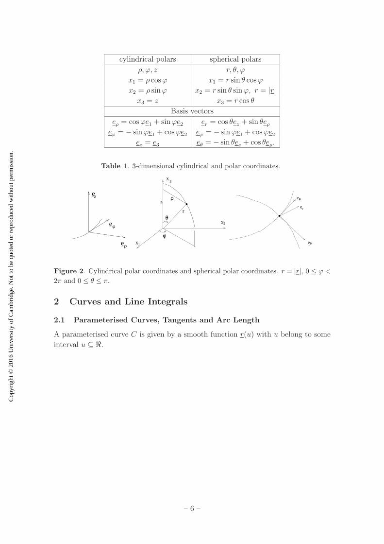
cylindrical polars spherical polars
ρ, ϕ, z r, θ, ϕ
x1 = ρ cosϕ x1 = r sin θ cosϕ
x2 = ρ sinϕ x2 = r sin θ sinϕ, r = |r|x3 = z x3 = r cos θ
Basis vectors
eρ = cosϕe1 + sinϕe2 er = cos θez + sin θeρeϕ = − sinϕe1 + cosϕe2 eϕ = − sinϕe1 + cosϕe2
ez = e3 eθ = − sin θez + cos θeρ.
Table 1. 3-dimensional cylindrical and polar coordinates.
����������������
����������������
��������������������������������
e
e
ez
ρ
φ
����
x
r
x1
2
x3
z
φ
θ
ρ
����
��
��
����
e
e
e
r
θ
φ
Figure 2. Cylindrical polar coordinates and spherical polar coordinates. r = |r|, 0 ≤ ϕ <2π and 0 ≤ θ ≤ π.
2 Curves and Line Integrals
2.1 Parameterised Curves, Tangents and Arc Length
A parameterised curve C is given by a smooth function r(u) with u belong to some
interval u ⊆ ℜ.
– 6 –

Cop
yrig
ht ©
201
6 U
nive
rsity
of C
ambr
idge
. Not
to b
e qu
oted
or
repr
oduc
ed w
ithou
t per
mis
sion
.
Examples:
1. r(u) = ui+ u2j + u3k for −∞ < u <∞, a curve without end-points.
2. r(u) = 2 cos ui+ sin uj + 3k where 0 ≤ u ≤ π, a curve with end-points.
This is a parameterisation of x2/4 + y2 = 1, y ≥ 0, z = 3.
0
r(u+ u)r(u)
Cr’(u)
r
δ
δ
The derivative r′(u) is a vector tangent to the curve at each point, provided it is
not zero. The parameterisation is called regular if r′(u) 6= 0. We will assume this
holds except perhaps at isolated points, so that the curve can always be divided into
segments on which the parameterisation is regular.
– 7 –

Cop
yrig
ht ©
201
6 U
nive
rsity
of C
ambr
idge
. Not
to b
e qu
oted
or
repr
oduc
ed w
ithou
t per
mis
sion
.
The arc length s measured along C, from some fixed point satisfies
δs = |δr|+ o(|δr|) = |r′(u)δu|+ o(δu) (2.1)
⇒ ds
du= ±
∣∣∣∣
dr
du
∣∣∣∣= ±|r′(u)|. (2.2)
The sign fixes the direction of measuring s, for increasing or decreasing u.
Example: A helix r(u) = (3 cos u, 3 sin u, 4u)⇒ r′(u) = (−3 sin u, 3 cos u, 4).
dsdu
= |r′(u)| =√32 + 42 = 5. Thus the arc length, measured from r(0) = 3i to
r(u) (u > 0) is s(u) = 5u. Hence, the distance from r(0) = 3i to r(2π) = 3i+ 8πk is
s(2π) = 10π.
The parameterisation of a curve can be changed: take u ↔ u invertible and
smooth (each is a smooth function of the other). The chain rule implies that
dr
du=dr
du/du
du
so the tangent vector changes size, but not direction. Choosing u = s, the arc length,
gives a tangent vector t = drds
of unit length along the direction of increasing s.
ds = ±|r′(u)|du is a scalar line element on C.
2.2 Line Integrals of Vector Fields
2.2.1 Definitions and Examples
Let C be a smooth curve r(u) with end points r(α) = a and r(β) = b, so that u runs
over an interval with ends α and β. A choice of orientation is a direction a→ b along
C. The line integral of a smooth vector field F (r) along C with this orientation is
defined by∫
C
F (r) · dr =∫ β
α
F (r(u)) · r′(u)du. (2.3)
– 8 –

Cop
yrig
ht ©
201
6 U
nive
rsity
of C
ambr
idge
. Not
to b
e qu
oted
or
repr
oduc
ed w
ithou
t per
mis
sion
.
This can be regarded as the limit of a sum over small displacements corresponding
to dividing the interval for u into small segments.
a
b
a
b
C C
F F
Each term is
F (r) · δr = F (r(u)) · drdu
+ o(δu).
The left hand side does not depend upon the parameterisation, and so neither does
Eq. 2.3. This can also be checked by the chain rule:
F (r) · drdudu = F (r) · dr
dudu.
Using components, with r = xiei and F = Fiei, the line integral is∫
CFidxi =
∫ β
αFi
dxidu
du.
dr = r′(u)du is the line element on C.
Examples: F (r) = (xey, z2, xy), so∫
CF · dr =
∫
Cxey dx+ z2 dy + xy dz.
C
C
b=(1,1,1)
a=(0,0,0)
1
2
u=0
u=1
We define C1 : r(u) = (u, u2, u3) ⇒ r′(u) = (1, 2u, 3u2). On C1, F (r) =
(ueu2
, u6, u3). Hence
∫
C1
F · dr =∫ 1
0
F · r′(u) du =
∫ 1
0
ueu2
+ 2u7 + 3u5 du = e/2 + 1/4.
For C2 : r(t) = (t, t, t) ⇒ r′(t) = (1, 1, 1) (we are now using t as the independent
variable). On C2, F (r(t)) = (tet, t2, t2). Hence
∫
C2
F · dr =∫ 1
0
(tet + 2t2) dt = [tet]10 −∫ 1
0
et dt+ 2/3 = 5/3.
– 9 –
Cop
yrig
ht ©
201
6 U
nive
rsity
of C
ambr
idge
. Not
to b
e qu
oted
or
repr
oduc
ed w
ithou
t per
mis
sion
.
A closed curve has b = a. The line integral is sometimes then written∮
CF · dr
and is called the circulation of F around C.
2.2.2 Comments
1.∫
CF · dr depends on C in general and not just upon the end points a and b.
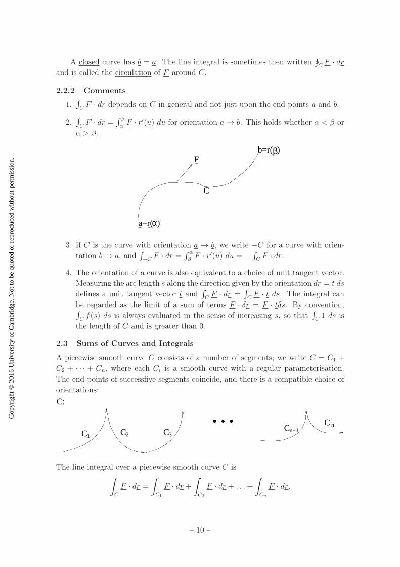
2.∫
CF · dr =
∫ β
αF · r′(u) du for orientation a→ b. This holds whether α < β or
α > β.
C
Fb=r( )
α
β
a=r( )
3. If C is the curve with orientation a → b, we write −C for a curve with orien-
tation b→ a, and∫
−C F · dr =∫ α
βF · r′(u) du = −
∫
CF · dr.
4. The orientation of a curve is also equivalent to a choice of unit tangent vector.
Measuring the arc length s along the direction given by the orientation dr = t ds
defines a unit tangent vector t and∫
CF · dr =
∫
CF · t ds. The integral can
be regarded as the limit of a sum of terms F · δr = F · tδs. By convention,∫
Cf(s) ds is always evaluated in the sense of increasing s, so that
∫
C1 ds is
the length of C and is greater than 0.
2.3 Sums of Curves and Integrals
A piecewise smooth curve C consists of a number of segments; we write C = C1 +
C2 + · · · + Cn, where each Ci is a smooth curve with a regular parameterisation.
The end-points of successfive segments coincide, and there is a compatible choice of
orientations:
������������������������
C C C CC
C:
1 2 3n−1
n
The line integral over a piecewise smooth curve C is∫
C
F · dr =∫
C1
F · dr +∫
C2
F · dr + . . .+
∫
Cn
F · dr.
– 10 –
Cop
yrig
ht ©
201
6 U
nive
rsity
of C
ambr
idge
. Not
to b
e qu
oted
or
repr
oduc
ed w
ithou
t per
mis
sion
.
The parameterisations on each Ci can be chosen independently.
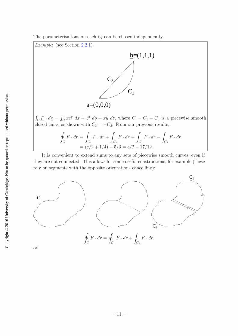
Example: (see Section 2.2.1)
C
C
b=(1,1,1)
a=(0,0,0)
1
3
∫
CF · dr =
∫
Cxey dx + z2 dy + xy dz, where C = C1 + C3 is a piecewise smooth
closed curve as shown with C3 = −C2. From our previous results,
∮
C
F · dr =
∫
C1
F · dr +∫
C3
F · dr =∫
C1
F · dr −∫
C2
F · dr
= (e/2 + 1/4)− 5/3 = e/2− 17/12.
It is convenient to extend sums to any sets of piecewise smooth curves, even if
they are not connected. This allows for some useful constructions, for example (these
rely on segments with the opposite orientations cancelling):
C
C
C
2
1
∮
C
F · dr =∮
C1
F · dr +∮
C2
F · dr.
or
– 11 –

Cop
yrig
ht ©
201
6 U
nive
rsity
of C
ambr
idge
. Not
to b
e qu
oted
or
repr
oduc
ed w
ithou
t per
mis
sion
.
C
C
C1
2
2.4 Gradients and Exact Differentials
2.4.1 Line Integrals and Gradients
If F = ∇f for some scalar field f(r) then∫
C
F · dr = f(b)− f(a), (2.4)
for any curve C from a to b.
a
b
C
Proof:∫
C
F · dr =∫
C
∇f · dr =∫ β
α
∇f · drdu
du
for any parameterisation of C with a = r(α) and b = r(β).
=
∫ β
α
d
du(f(r(u))) du
by the chain rule, see section 1.1.3,
= [f(r(u))]βα = f(b)− f(a),
as required.
Note that
• When F is a gradient, the line integral depends only on the end points, not on
the curve joining them.
• When C is a closed curve,∮
CF · dr = 0 if F is a gradient.
• If F = ∇f , F is called a conservative vector field. There are a number of
alternative definitions which are equivalent (with suitable assumptions) - see
later.
– 12 –
Cop
yrig
ht ©
201
6 U
nive
rsity
of C
ambr
idge
. Not
to b
e qu
oted
or
repr
oduc
ed w
ithou
t per
mis
sion
.
2.4.2 Differentials
It is often convenient to work with differentials F · dr = Fi dxi as objects that can
be integrated along curves. Such a differential is called exact if it has the form
df = ∇f · dr = ∂f∂xi
dxi. So F = ∇f ⇔ Fi =∂f∂xi⇔ Fi dxi = df is exact. To test
if this holds, we can use the necessary condition ∂Fi
∂xj=
∂Fj
∂xi(since both are equal to
∂2f∂xi∂xj
for ‘nice’ functions). We will see later that, locally, this is also sufficient. For
an exact differential, Eq. 2.4 is∫
C
F · dr =∫
C
df = f(b)− f(a).
Differentials can be manipulated using
d(λf + µg) = λdf + µdg
for constants µ and λ. There is also a Leibniz rule
d(fg) = (df)g + f(dg).
Using these, it may be possible to find f by inspection.
Example:
∫
C
(3x2y sin z dx+ x3 sin z dy + x3y cos z dz) =
∫
C
d(x3y sin z) =[x3y sin z
]b
a= 1
if a = (0, 0, 0) and b = (1, 1, π/2), for instance.
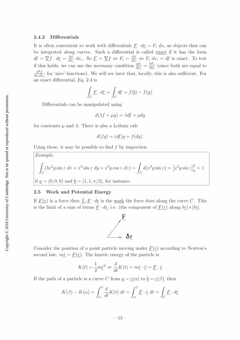
2.5 Work and Potential Energy
If F (r) is a force then∫
CF · dr is the work the force does along the curve C. This
is the limit of a sum of terms F · dr, i.e. (the component of F (r) along δr)×|δr|.
F
rδ
Consider the position of a point particle moving under F (r) according to Newton’s
second law: mr = F (r). The kinetic energy of the particle is
K(t) =1
2mr2 ⇒ d
dtK(t) = mr · r = F · r
If the path of a particle is a curve C from a = r(α) to b = r(β), then
K(β)−K(α) =
∫ β
α
d
dtK(t) dt =
∫ β
α
F · r dt =∫
C
F · dr
– 13 –
Cop
yrig
ht ©
201
6 U
nive
rsity
of C
ambr
idge
. Not
to b
e qu
oted
or
repr
oduc
ed w
ithou
t per
mis
sion
.
i.e. the change in the kinetic energy is equal to the work done by the force.
For a conservative force, F = −∇V , where V (r) is the potential energy (setting
f = −V in Eq. 2.4),∫
CF · dr = V (a) − V (b), or the work done is equal to the loss
in potential energy. So, in this case,
K(β) + V (r(β)) = K(α) + V (r(α)),
i.e. the total energy K + V is conserved (in other words, it is constant during the
motion).
3 Integration in ℜ2 and ℜ3
3.1 Integrals over subsets of ℜ2
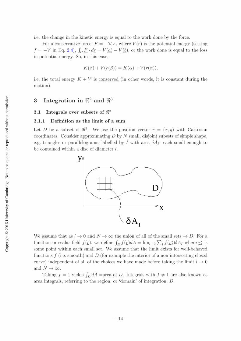
3.1.1 Definition as the limit of a sum
Let D be a subset of ℜ2. We use the position vector r = (x, y) with Cartesian
coordinates. Consider approximating D by N small, disjoint subsets of simple shape,
e.g. triangles or parallelograms, labelled by I with area δAI : each small enough to
be contained within a disc of diameter l.
δA
x
y
I
D
We assume that as l → 0 and N →∞ the union of all of the small sets → D. For a
function or scalar field f(r), we define∫
Df(r)dA = liml→0
∑
I f(r∗I)δAI where r∗I is
some point within each small set. We assume that the limit exists for well-behaved
functions f (i.e. smooth) and D (for example the interior of a non-intersecting closed
curve) independent of all of the choices we have made before taking the limit l → 0
and N →∞.
Taking f = 1 yields∫
DdA =area of D. Integrals with f 6= 1 are also known as
area integrals, referring to the region, or ‘domain’ of integration, D.
– 14 –

Cop
yrig
ht ©
201
6 U
nive
rsity
of C
ambr
idge
. Not
to b
e qu
oted
or
repr
oduc
ed w
ithou
t per
mis
sion
.
3.1.2 Evaluation as multiple integrals
Area integrals can be expressed as successive integrals over the coordinates x and
y as follows: choose the small sets in the definition to be rectangles, each of size
δAI = δxδy. Summing over subsets in a narrow horizontal strip with y and δy
fixed and taking δx → 0 gives a contribution δy∫
xyf(x, y) dx with range xy =
{x : (x, y) ∈ D}. Then, summing over all such strips and taking δy → 0 gives∫
Df(x, y) dA =
∫
Y
(∫
xyf(x, y) dx
)
dy where Y is the range of all y in D:
x
y
Y
x
y+ y
y
y
δ
Alternatively, we can first sum over subsets in a narrow vertical strip with x and
δx fixed and take δy → 0 to get δx∫
Yxf(x, y) dy with range Yx = {y : (x, y) ∈
D}. Then, we sum over all such strips and take δx → 0 to get∫
Df(x, y) dA =
∫
X
(∫
Yxf(x, y)dy
)
dx, where X is the range of all x in D:
x x+ xδ x
y
X
Yx
We can summarise all of this by the statement that the area element is dA = dx dy
in Cartesian coordinates.
– 15 –
Cop
yrig
ht ©
201
6 U
nive
rsity
of C
ambr
idge
. Not
to b
e qu
oted
or
repr
oduc
ed w
ithou
t per
mis
sion
.
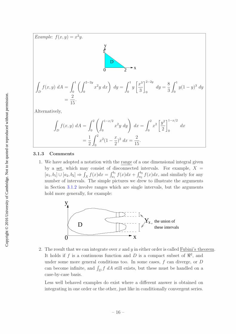
Example: f(x, y) = x2y.
x
y1
20
D
∫
D
f(x, y) dA =
∫ 1
0
(∫ 2−2y
0
x2y dx
)
dy =
∫ 1
0
y
[x3
3
]2−2y
0
dy =8
3
∫ 1
0
y(1− y)3 dy
=2
15.
Alternatively,
∫
D
f(x, y) dA =
∫ 2
0
(∫ 1−x/2
0
x2y dy
)
dx =
∫ 2
0
x2[y2
2
]1−x/2
0
dx
=1
2
∫ 2
0
x2(1− x
2)2 dx =
2
15.
3.1.3 Comments
1. We have adopted a notation with the range of a one dimensional integral given
by a set, which may consist of disconnected intervals. For example, X =
[a1, b1] ∪ [a2, b2]⇒∫
Xf(x)dx =
∫ b1a1f(x)dx+
∫ b2a2f(x)dx, and similarly for any
number of intervals. The simple pictures we drew to illustrate the arguments
in Section 3.1.2 involve ranges which are single intervals, but the arguments
hold more generally, for example:
0 x
y
DYx ,
these intervals
the union of
2. The result that we can integrate over x and y in either order is called Fubini’s theorem.
It holds if f is a continuous function and D is a compact subset of ℜ2, and
under some more general conditions too. In some cases, f can diverge, or D
can become infinite, and∫
Df dA still exists, but these must be handled on a
case-by-case basis.
Less well behaved examples do exist where a different answer is obtained on
integrating in one order or the other, just like in conditionally convergent series.
– 16 –

Cop
yrig
ht ©
201
6 U
nive
rsity
of C
ambr
idge
. Not
to b
e qu
oted
or
repr
oduc
ed w
ithou
t per
mis
sion
.
3. In the special case f(x, y) = g(x)h(y) andD = {(x, y) : a ≤ x ≤ b, c ≤ y ≤ d},∫
Df(x, y) dx dy =
∫ b
ag(x)dx
∫ d
ch(y)dy.
4. By plotting the graph of z = f(x, y) in three dimensions, we get a surface and∫
Df(x, y) dA can be interpreted as the volume beneath it:
D
x
y
z
3.2 Change of Variables for an Integral in ℜ2
Consider a smooth invertible transformation (x, y) ↔ (u, v) with regions D and D′
in one-to-one correspondence:
x
y
u
v
D D’
Then for a function (or scalar field) f ,∫
Df(x, y) dx dy =
∫
D′f(x(u, v), y(u, v))|J | du dv,
where
J =∂(x, y)
∂(u, v)=
∣∣∣∣
∂x∂u
∂x∂v
∂y∂u
∂y∂v
∣∣∣∣
is the Jacobian. In the formula, |J | is the modulus of the Jacobian.
Proof in outline: write∫
D′as the limit of the sum of rectangles of area δA′ = δuδv
in the (u, v) plane. Each rectangle is mapped approximately to a parallelogram of
area A = |J |δuδv in the (x, y) plane, since up to o−terms,(δx
δy
)
=
(∂x∂u
∂x∂v
∂y∂u
∂y∂v
)(δu
δv
)
,
– 17 –
Cop
yrig
ht ©
201
6 U
nive
rsity
of C
ambr
idge
. Not
to b
e qu
oted
or
repr
oduc
ed w
ithou
t per
mis
sion
.
and |J | is the factor by which the areas are related. Summing over parallelograms in
the (x, y) plane gives the integral over D as claimed, with the Jacobian factor giving
the correct area for each parallelogram. The result can be summarised as
dA =
∣∣∣∣
∂(x, y)
∂(u, v)
∣∣∣∣du dv.
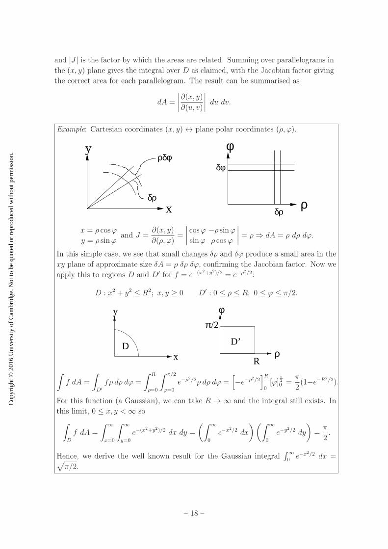
Example: Cartesian coordinates (x, y)↔ plane polar coordinates (ρ, ϕ).
x
y
ρ
φ
δρ
ρδφ
δρ
δφ
x = ρ cosϕ
y = ρ sinϕand J =
∂(x, y)
∂(ρ, ϕ)=
∣∣∣∣
cosϕ −ρ sinϕsinϕ ρ cosϕ
∣∣∣∣= ρ⇒ dA = ρ dρ dϕ.
In this simple case, we see that small changes δρ and δϕ produce a small area in the
xy plane of approximate size δA = ρ δρ δϕ, confirming the Jacobian factor. Now we
apply this to regions D and D′ for f = e−(x2+y2)/2 = e−ρ2/2:
D : x2 + y2 ≤ R2; x, y ≥ 0 D′ : 0 ≤ ρ ≤ R; 0 ≤ ϕ ≤ π/2.
x
y
ρ
φ
D D’
R
π/2
∫
f dA =
∫
D′
fρ dρ dϕ =
∫ R
ρ=0
∫ π/2
ϕ=0
e−ρ2/2ρ dρ dϕ =
[
−e−ρ2/2]R
0[ϕ]
π2
0 =π
2(1−e−R2/2).
For this function (a Gaussian), we can take R → ∞ and the integral still exists. In
this limit, 0 ≤ x, y <∞ so
∫
D
f dA =
∫ ∞
x=0
∫ ∞
y=0
e−(x2+y2)/2 dx dy =
(∫ ∞
0
e−x2/2 dx
)(∫ ∞
0
e−y2/2 dy
)
=π
2.
Hence, we derive the well known result for the Gaussian integral∫∞0e−x
2/2 dx =√
π/2.
– 18 –
Cop
yrig
ht ©
201
6 U
nive
rsity
of C
ambr
idge
. Not
to b
e qu
oted
or
repr
oduc
ed w
ithou
t per
mis
sion
.
3.3 Generalisation to ℜ3
3.3.1 Definitions
Let a volume V ∈ ℜ3 and a position vector r = (x, y, z). We approximate V by
N small disjoint subsets of simple shape (for example, cuboids) labelled by I with
volume δVI , each contained within a solid sphere of diameter l. We assume that as
l→ 0 and N →∞, the union of the small subsets tends to V . Then, the integral of
a function (or scalar field) f(r) over V is defined
∫
V
f(r) dV = liml→0
∑
I
f(r∗I)δVI ,
where r∗I is any chosen point in each small subset.
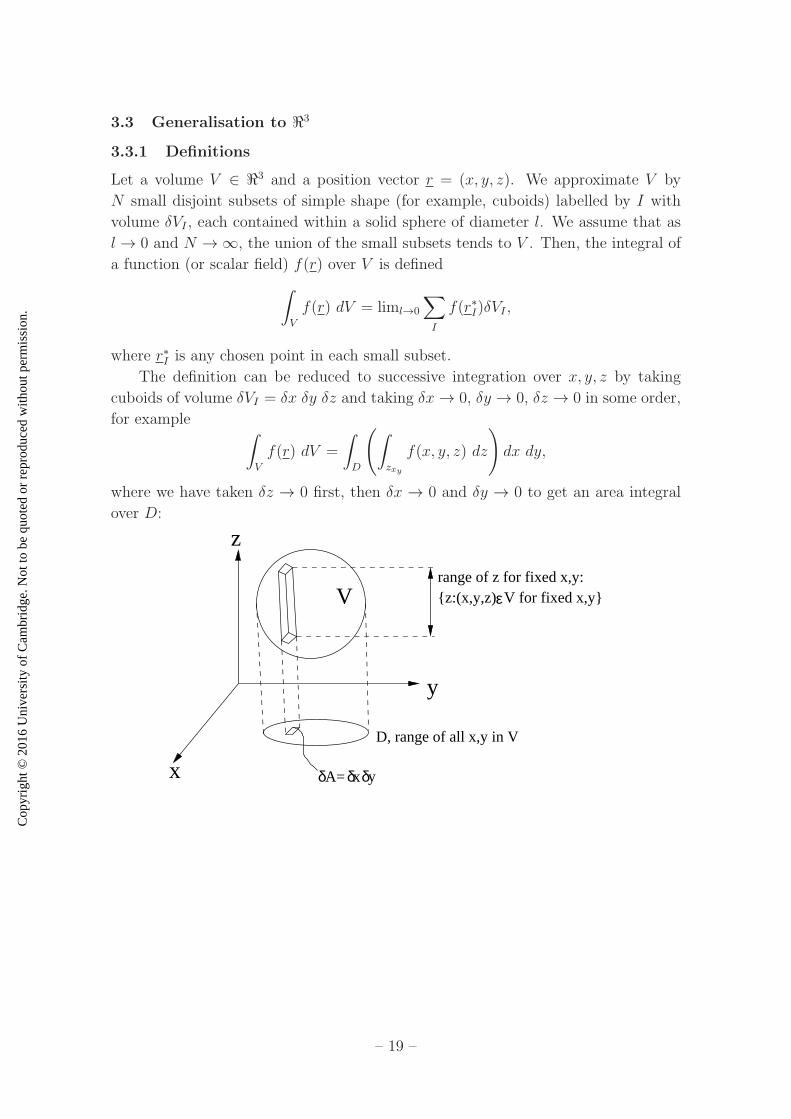
The definition can be reduced to successive integration over x, y, z by taking
cuboids of volume δVI = δx δy δz and taking δx→ 0, δy → 0, δz → 0 in some order,
for example∫
V
f(r) dV =
∫
D
(∫
zxy
f(x, y, z) dz
)
dx dy,
where we have taken δz → 0 first, then δx → 0 and δy → 0 to get an area integral
over D:
Vrange of z for fixed x,y:{z:(x,y,z) V for fixed x,y}
D, range of all x,y in V
A= x y
ε
δ δ δx
y
z
– 19 –

Cop
yrig
ht ©
201
6 U
nive
rsity
of C
ambr
idge
. Not
to b
e qu
oted
or
repr
oduc
ed w
ithou
t per
mis
sion
.
Alternatively,∫
Vf(r) dV =
∫
z(∫
Dzf(x, y, z) dx dy)dz, i.e. take δx and δy to zero
first to get an area integral over slice Dz, then sum over slices and take δz → 0:
V
x
y
z
Dz’ ,the range of all (x,y) such that(x,y,z) V for fixed z.
range of all z in V
zδ
ε
Taking f = 1 gives∫
VdV =volume of V . f 6= 1 are also known as volume
integrals. Such integrals arise with f(r) being the density for some quantity, for
example mass, charge or probability, often denoted ρ. Then, ρ(r) is the amount of
the quantity in a small volume δV at r.∫
Vρ(r) dV is the total amount of the quantity
in V . To summarise: the volume element in Cartesian coordinates dV = dx dy dz.
3.3.2 Change of Variables in ℜ3
Consider an invertible transformation (x, y, z) ↔ (u, v, w), which is smooth both
ways, with regions V and V ′ in 1 : 1 correspondence. Then, for a function f ,∫
Vf dx dy dz =
∫
V ′f |J | du dv dw where
J =∂(x, y, z)
∂(u, v, w)=
∣∣∣∣∣∣
∂x∂u
∂x∂v
∂x∂w
∂y∂u
∂y∂v
∂y∂w
∂z∂u
∂z∂v
∂z∂w
∣∣∣∣∣∣
is the Jacobian.
The justification (an informal proof) is similar to the 2-dimensional case: given
a small cuboid with sides δu, δv, δw respectively, we get an approximate small paral-
lelapiped of volume |J |δuδvδw in (x, y, z) space, and we can use these as small sets
in the definition of the integral, hence the result.
Important special cases are cylindrical polar or spherical polar coordinates, as
in Section 1.3. For cylindrical polar coordinates
x = ρ cosϕ, y = ρ sinϕ, z, (3.1)
which means∂(x, y, z)
∂(ρ, ϕ, z)= ρ⇒ dV = ρdρ dϕ dz.
– 20 –

Cop
yrig
ht ©
201
6 U
nive
rsity
of C
ambr
idge
. Not
to b
e qu
oted
or
repr
oduc
ed w
ithou
t per
mis
sion
.
On the other hand, in spherical polar coordinates,
x = r sin θ cosϕ, y = r sin θ sinϕ, z = r cos θ. (3.2)
i.e.∂(x, y, z)
∂(r, θ, ϕ)= r2 sin θ ⇒ dV = r2 sin θdr dθ dϕ.
In summary, for a general coordinate system, the volume element is:
dV =
∣∣∣∣
∂(x, y, z)
∂(u, v, w)
∣∣∣∣du dv dw.
3.3.3 Examples
Example: f(r) is spherically symmetric and V is a sphere of radius a.
∫
V
f dV =
∫ a
r=0
∫ π
θ=0
∫ 2π
ϕ=0
f(r)r2 sin θ dr dθ dϕ =
∫ a
0
dr
∫ π
0
dθ
∫ 2π
0
dϕ r2f(r) sin θ
=
∫ a
0
dr r2f(r)[− cos θ]π0 [ϕ]2π0 = 4π
∫ a
0
f(r)r2 dr,
a useful general result. We can understand it as the sum of spherical shells of
thickness δr and volume 4πr2δr, taking δr → 0. Note that taking f = 1 gives the
volume of a sphere, 4πa3/3.
Example: Consider the volume within a sphere of radius a with a cylinder of radius
b removed (where b < a). Thus V : x2 + y2 + z2 ≤ a2 and x2 + y2 ≥ b2.
x
y
z
a z=(a − )2 21/2
ρρ
In cylindrical polar coordinates ρ, ϕ, z, dV = ρ dρ dϕ dz and V : b ≤ ρ ≤ a,
0 ≤ ϕ ≤ 2π and −√
a2 − ρ2 ≤ z ≤√
a2 − ρ2.
∫
V
dV =
∫ b
ρ=a
∫ 2π
ϕ=0
∫ z=√a2−ρ2
z=−√a2−ρ2
ρ dρ dϕ dz = 2π
∫ a
b
dρ 2ρ√
a2 − ρ2 = 4π
3(a2 − b2)3/2
– 21 –
Cop
yrig
ht ©
201
6 U
nive
rsity
of C
ambr
idge
. Not
to b
e qu
oted
or
repr
oduc
ed w
ithou
t per
mis
sion
.
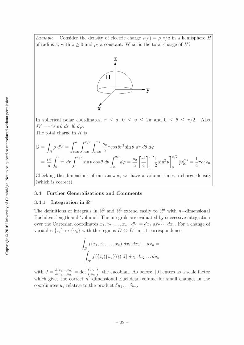
Example: Consider the density of electric charge ρ(r) = ρ0z/a in a hemisphere H
of radius a, with z ≥ 0 and ρ0 a constant. What is the total charge of H?
x
y
z
H
In spherical polar coordinates, r ≤ a, 0 ≤ ϕ ≤ 2π and 0 ≤ θ ≤ π/2. Also,
dV = r2 sin θ dr dθ dϕ.
The total charge in H is
Q =
∫
H
ρ dV =
∫ a
r=0
∫ π/2
θ=0
∫ 2π
ϕ=0
ρ0ar cos θr2 sin θ dr dθ dϕ
=ρ0a
∫ a
0
r3 dr
∫ π/2
0
sin θ cos θ dθ
∫ 2π
0
dϕ =ρ0a
[r4
4
]a
0
[1
2sin2 θ
]π/2
0
[ϕ]2π0 =1
4πa3ρ0.
Checking the dimensions of our answer, we have a volume times a charge density
(which is correct).
3.4 Further Generalisations and Comments
3.4.1 Integration in ℜn
The definitions of integrals in ℜ2 and ℜ3 extend easily to ℜn with n−dimensional
Euclidean length and ‘volume’. The integrals are evaluated by successive integration
over the Cartesian coordinates x1, x2, . . . , xn : dV = dx1 dx2 · · · dxn. For a change of
variables {xi} ↔ {ua} with the regions D ↔ D′ in 1:1 correspondence,
∫
D
f(x1, x2, . . . , xn) dx1 dx2 . . . dxn =∫
D′
f({xi({ua})})|J | du1 du2 . . . dun
with J = ∂(x1,...,xn)∂(u1,...,un)
= det(∂xiua
)
, the Jacobian. As before, |J | enters as a scale factor
which gives the correct n−dimensional Euclidean volume for small changes in the
coordinates ua relative to the product δu1 . . . δun.
– 22 –

Cop
yrig
ht ©
201
6 U
nive
rsity
of C
ambr
idge
. Not
to b
e qu
oted
or
repr
oduc
ed w
ithou
t per
mis
sion
.
3.4.2 Change of variables for the case n = 1
For a single variable n = 1, the Jacobian is just J = dx/du and the general formula
reads ∫
D
f(x)dx =
∫
D′
f(x(u))
∣∣∣∣
dx
du
∣∣∣∣du.
The modulus of dx/du is correct because of our natural convention about integrating
over subsets D and D′.
For example, suppose D is the interval a ≤ x ≤ b so∫
Df(x) dx =
∫ b
af(x) dx.
Let u = α, β correspond to x = a, b, respectively. Since x ↔ u is invertible and
smooth in both directions, dxdu6= 0. Either α < β and dx
du> 0, in which case
∫
D′f |dx
du| du =
∫ β
αf dxdu
du or α > β and dxdu
< 0, so∫
D′f |dx
du| du =
∫ α
βf(−dx
du) du.
Either way, the formula yields∫ b
af(x) dx =
∫ β
αf(x(u))dx
dudu, a familiar result.
3.4.3 Vector valued integrals
Because limits apply to vectors as well as scalars, we can define for instance∫
VF (r)dV
in a similar way to∫
Vf(r)dV as the limit of a sum over contributions from small vol-
umes. With Cartesian components F (r) = Fi(r)ei, we have∫
VF (r)dV =
(∫
VFi(r)dV
)ei,
i.e. we can integrate component by component.
Take the case of ρ(r) being a mass density for a body occupying volume V .
Then,
M =
∫
V
ρ(r)dV
is the total mass and
R =1
M
∫
V
rρ(r)dV
is the centre of mass. This generalises definitions for a set of point particles at
positions rα (α labels the particle, not the component here):
M =∑
α
mα, R =1
M
∑
α
marα.
– 23 –

Cop
yrig
ht ©
201
6 U
nive
rsity
of C
ambr
idge
. Not
to b
e qu
oted
or
repr
oduc
ed w
ithou
t per
mis
sion
.
Example: Consider a solid hemisphere H with r ≤ a and z ≥ 0, with uniform density
ρ. The total mass M =∫
Hρ dV = 2πa3ρ/3. If we put R = (X, Y, Z):
X =1
M
∫
H
xρ dV =ρ
M
∫ a
r=0
∫ π/2
θ=0
∫ 2π
ϕ=0
xr2 sin θ dr dθ dϕ
=ρ
M
∫ a
0
r3 dr
∫ π/2
0
sin2 θ dθ�������∫ 2π
0
cosϕ dϕ = 0.
Y = 0 in a similar way.
Z =ρ
M
∫ a
0
r3 dr
∫ π/2
0
sin θ cos θdθ
∫ 2π
0
dϕ =ρ
M
a4
4
1
22π =
3a
8,
i.e. the centre of mass is at R = (0, 0, 3a/8).
4 Surfaces and Surface Integrals
4.1 Surfaces and Normals
For an appropriate smooth function f on ℜ3 and a suitable constant c, the equation
f(r) = c defines a smooth surface S. Consider any curve r(u) in S.
drdu
f
By the chain rule, dduf(r(u)) = ∇f · dr
du. This is zero, since the curve is in S and
f does not change along it. At any r on S with ∇f 6= 0, there exist two linearly
independent tangent directions ⊥ to ∇f . Hence
1. In the neighbourhood of this point, the equation indeed describes a surface (it
has two independent tangent directions).
2. ∇f is normal to the surface at this point.
– 24 –

Cop
yrig
ht ©
201
6 U
nive
rsity
of C
ambr
idge
. Not
to b
e qu
oted
or
repr
oduc
ed w
ithou
t per
mis
sion
.
Examples: f(r) = x2 + y2 + z2 = c. For c > 0, this describes a sphere of radius√c.
∇f = 2(x, y, z) = 2r.
x
y
z
f
Taking f(r) = x2 + y2 − z2 = c results in a hyperboloid for c > 0. ∇f = 2(x, y,−z).
x
y
z
f
For c = 0, the surface degenerates to a single point 0 in the first case, and to a double
cone in the second (it is singular at the apex 0, where ∇f = 0.
x
y
z
c=0
A surface S can be defined to have a boundary ∂S consisting of a piecewise
smooth closed curve. Defining S as above but with z ≥ 0, ∂S is the circle x2+y2 = c
and z = 0 in the first two cases. A surface is bounded if it can be contained within
some solid sphere, and unbounded otherwise. A bounded surface with no boundary
is called closed.
At each point on a surface, there is a unit normal n (a normal of unit length) that
is unique up to a sign. The surface is called orientable if there is a consistent choice
of unit normal n which varies smoothly. We shall deal exclusively with orientable
surfaces, which rules out examples like the Mobius band:
– 25 –
Cop
yrig
ht ©
201
6 U
nive
rsity
of C
ambr
idge
. Not
to b
e qu
oted
or
repr
oduc
ed w
ithou
t per
mis
sion
.
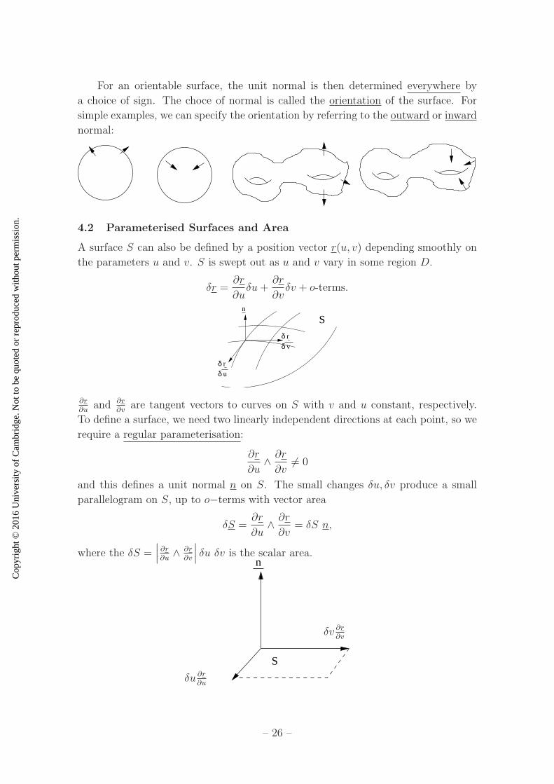
For an orientable surface, the unit normal is then determined everywhere by
a choice of sign. The choce of normal is called the orientation of the surface. For
simple examples, we can specify the orientation by referring to the outward or inward
normal:
4.2 Parameterised Surfaces and Area
A surface S can also be defined by a position vector r(u, v) depending smoothly on
the parameters u and v. S is swept out as u and v vary in some region D.
δr =∂r
∂uδu+
∂r
∂vδv + o-terms.
Sn
r
v
r
u
δδ
δδ
∂r∂u
and ∂r∂v
are tangent vectors to curves on S with v and u constant, respectively.
To define a surface, we need two linearly independent directions at each point, so we
require a regular parameterisation:
∂r
∂u∧ ∂r∂v6= 0
and this defines a unit normal n on S. The small changes δu, δv produce a small
parallelogram on S, up to o−terms with vector area
δS =∂r
∂u∧ ∂r∂v
= δS n,
where the δS =∣∣∣∂r∂u∧ ∂r
∂v
∣∣∣ δu δv is the scalar area.
δu ∂r∂u
n
S
δv ∂r∂v
– 26 –
Cop
yrig
ht ©
201
6 U
nive
rsity
of C
ambr
idge
. Not
to b
e qu
oted
or
repr
oduc
ed w
ithou
t per
mis
sion
.
Note that with these conventions, the choice of the unit normal is determined
by the order of the parameters u and v. By summing and taking limits, the area of
S is ∫
S
dS =
∫
D
∣∣∣∣
∂r
∂u∧ ∂r∂v
∣∣∣∣du dv,
where dS =∣∣∣∂r∂u∧ ∂r
∂v
∣∣∣ du dv is the scalar area element.
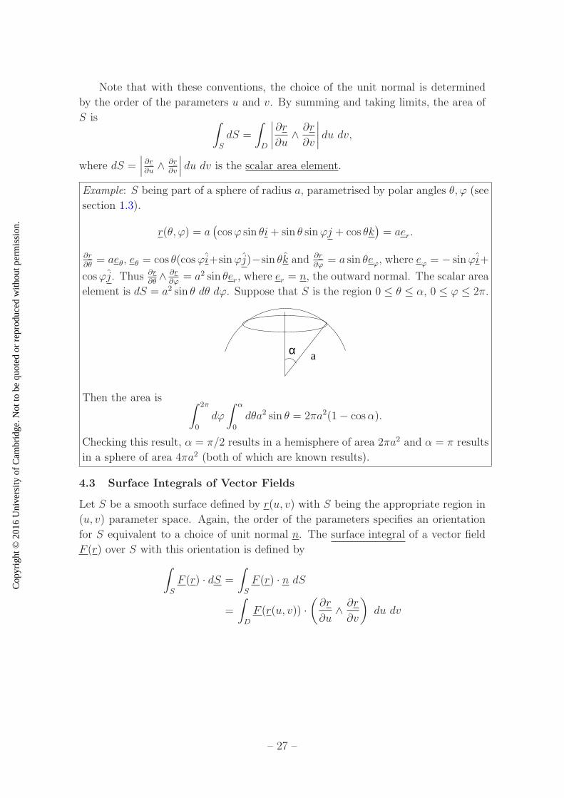
Example: S being part of a sphere of radius a, parametrised by polar angles θ, ϕ (see
section 1.3).
r(θ, ϕ) = a(cosϕ sin θi+ sin θ sinϕj + cos θk
)= aer.
∂r∂θ
= aeθ, eθ = cos θ(cosϕi+sinϕj)−sin θk and ∂r∂ϕ
= a sin θeϕ, where eϕ = − sinϕi+
cosϕj. Thus ∂r∂θ∧ ∂r∂ϕ
= a2 sin θer, where er = n, the outward normal. The scalar area
element is dS = a2 sin θ dθ dϕ. Suppose that S is the region 0 ≤ θ ≤ α, 0 ≤ ϕ ≤ 2π.
α a
Then the area is ∫ 2π
0
dϕ
∫ α
0
dθa2 sin θ = 2πa2(1− cosα).
Checking this result, α = π/2 results in a hemisphere of area 2πa2 and α = π results
in a sphere of area 4πa2 (both of which are known results).
4.3 Surface Integrals of Vector Fields
Let S be a smooth surface defined by r(u, v) with S being the appropriate region in
(u, v) parameter space. Again, the order of the parameters specifies an orientation
for S equivalent to a choice of unit normal n. The surface integral of a vector field
F (r) over S with this orientation is defined by
∫
S
F (r) · dS =
∫
S
F (r) · n dS
=
∫
D
F (r(u, v)) ·(∂r
∂u∧ ∂r∂v
)
du dv
– 27 –

Cop
yrig
ht ©
201
6 U
nive
rsity
of C
ambr
idge
. Not
to b
e qu
oted
or
repr
oduc
ed w
ithou
t per
mis
sion
.
Sn
F
Sδ
D
u vδ δ
By writing the integral over D as the limit of a sum over small rectangles δuδv, the
integral over S becomes the limit of a sum of contributions
Fn
Sδ
F (r) · δS = F (r) · n δS
= F (r(u, v)) ·(∂r
∂u∧ ∂r∂v
)
δu δv + o-terms.
From the geometrical nature of the left hand side, the integral∫
SF ·dS is independent
of the parameterisation, for a given orientation. It is called the flux of F through S.
dS = ndS =∂r
∂u∧ ∂r∂v
du dv
is the vector area element.
Note that changing the orientation of S is equivalent to changing the sign of the
unit normal n, which is equivalent to changing the order of u and v in the definition
of S, which is also equivalent to changing the sign of any flux integral.
Example: For a sphere of radius a we found from r(θ, ϕ) in section 4.2 that ∂r∂θ
= aeθ,∂r∂ϕ
= a sin θeϕ. The vector area element is then dS = ndS = ∂r∂θ∧ ∂r
∂ϕdθ dϕ =
a2 sin θer dθ dϕ, where n = er = r/a, the outward normal.
The fluid flux through a surface provides a physical example. The velocity field
u(r) of a fluid gives the motion of any small volume of fluid at r.
u(r)
– 28 –
Cop
yrig
ht ©
201
6 U
nive
rsity
of C
ambr
idge
. Not
to b
e qu
oted
or
repr
oduc
ed w
ithou
t per
mis
sion
.
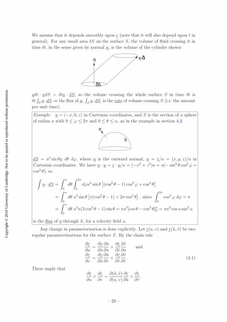
We assume that it depends smoothly upon r (note that it will also depend upon t in
general). For any small area δS on the surface S, the volume of fluid crossing it in
time δt, in the sense given by normal n, is the volume of the cylinder shown:
n u t
S
δ
δ
uδt · nδS = δtu · δS, so the volume crossing the whole surface S in time δt is
δt∫
Su ·dS ⇒ the flux of u,
∫
Su ·dS, is the rate of volume crossing S (i.e. the amount
per unit time).
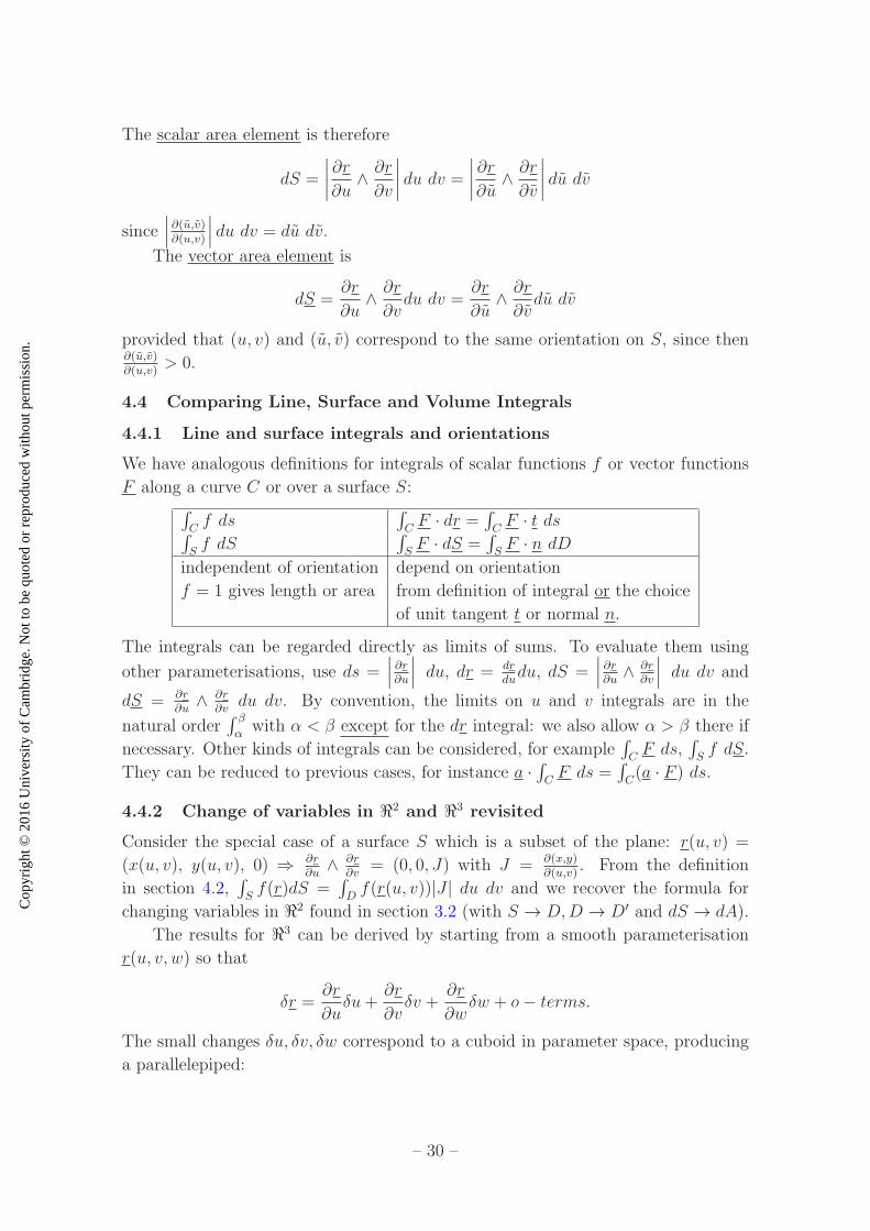
Example: u = (−x, 0, z) in Cartesian coordinates, and S is the section of a sphere
of radius a with 0 ≤ ϕ ≤ 2π and 0 ≤ θ ≤ α, as in the example in section 4.2.
n
S
dS = a2 sin θn dθ dϕ, where n is the outward normal, n = r/a = (x, y, z)/a in
Cartesian coordinates. We have n · u = r · u/a = (−x2 + z2)a = a(− sin2 θ cos2 ϕ +
cos2 θ), so
∫
u · dS =
∫ α
0
dθ
∫ 2π
0
dϕa3 sin θ[(cos2 θ − 1) cos2 ϕ+ cos2 θ
]
=
∫ α
0
dθ a3 sin θ[π(cos2 θ − 1) + 2π cos2 θ
], since
∫ 2π
0
cos2 ϕ dϕ = π
=
∫ α
0
dθ a3π(3 cos2 θ − 1) sin θ = πa3[cos θ − cos3 θ]α0 = πa3 cosα sin2 α
is the flux of u through S, for a velocity field u.
Any change in parameterisation is done explicitly. Let r(u, v) and r(u, v) be two
regular parameterisations for the surface S. By the chain rule
∂r
∂u=∂r
∂u
∂u
∂u+∂r
∂v
∂v
∂uand
∂r
∂v=∂r
∂u
∂u
∂v+∂r
∂v
∂v
∂v. (4.1)
These imply that∂r
∂u∧ ∂r∂v
=∂(u, v)
∂(u, v)
∂r
∂u∧ ∂r∂v.
– 29 –
Cop
yrig
ht ©
201
6 U
nive
rsity
of C
ambr
idge
. Not
to b
e qu
oted
or
repr
oduc
ed w
ithou
t per
mis
sion
.
The scalar area element is therefore
dS =
∣∣∣∣
∂r
∂u∧ ∂r∂v
∣∣∣∣du dv =
∣∣∣∣
∂r
∂u∧ ∂r∂v
∣∣∣∣du dv
since∣∣∣∂(u,v)∂(u,v)
∣∣∣ du dv = du dv.
The vector area element is
dS =∂r
∂u∧ ∂r∂vdu dv =
∂r
∂u∧ ∂r∂vdu dv
provided that (u, v) and (u, v) correspond to the same orientation on S, since then∂(u,v)∂(u,v)
> 0.
4.4 Comparing Line, Surface and Volume Integrals
4.4.1 Line and surface integrals and orientations
We have analogous definitions for integrals of scalar functions f or vector functions
F along a curve C or over a surface S:∫
Cf ds
∫
CF · dr =
∫
CF · t ds
∫
Sf dS
∫
SF · dS =
∫
SF · n dD
independent of orientation depend on orientation
f = 1 gives length or area from definition of integral or the choice
of unit tangent t or normal n.
The integrals can be regarded directly as limits of sums. To evaluate them using
other parameterisations, use ds =∣∣∣∂r∂u
∣∣∣ du, dr = dr
dudu, dS =
∣∣∣∂r∂u∧ ∂r
∂v
∣∣∣ du dv and
dS = ∂r∂u∧ ∂r
∂vdu dv. By convention, the limits on u and v integrals are in the
natural order∫ β
αwith α < β except for the dr integral: we also allow α > β there if
necessary. Other kinds of integrals can be considered, for example∫
CF ds,
∫
Sf dS.
They can be reduced to previous cases, for instance a ·∫
CF ds =
∫
C(a · F ) ds.
4.4.2 Change of variables in ℜ2 and ℜ3 revisited
Consider the special case of a surface S which is a subset of the plane: r(u, v) =
(x(u, v), y(u, v), 0) ⇒ ∂r∂u∧ ∂r
∂v= (0, 0, J) with J = ∂(x,y)
∂(u,v). From the definition
in section 4.2,∫
Sf(r)dS =
∫
Df(r(u, v))|J | du dv and we recover the formula for
changing variables in ℜ2 found in section 3.2 (with S → D,D → D′ and dS → dA).
The results for ℜ3 can be derived by starting from a smooth parameterisation
r(u, v, w) so that
δr =∂r
∂uδu+
∂r
∂vδv +
∂r
∂wδw + o− terms.
The small changes δu, δv, δw correspond to a cuboid in parameter space, producing
a parallelepiped:
– 30 –

Cop
yrig
ht ©
201
6 U
nive
rsity
of C
ambr
idge
. Not
to b
e qu
oted
or
repr
oduc
ed w
ithou
t per
mis
sion
.
δv ∂r∂v
δw ∂r∂w
δu ∂r∂u
of volume δV =∣∣∣∂r∂uδu · ∂r
∂vδv ∧ ∂r
∂wδw∣∣∣ = |J |δu δv δw. We deduce that the volume
element is dV = |J |du dv dw where J = ∂r∂u· ∂r∂v∧ ∂r∂w
= ∂(x,y,z)∂(u,v,w)
. This is an alternative
derivation of the result in section 3.3.
5 Geometry of Curves and Surfaces
5.1 Curves, Curvature and Normals
Let r(s) be a curve parameterised by the arc length s. Since t(s) = drds
is a unit
tangent vector, t2 = 1⇒ t · t′ = 0 specifies a direction normal to the curve if t′ 6= 0.
Let t′ = κn where the unit vector n(s) is called the principal normal and κ(s) is
called the curvature (we can make κ positive by choosing an appropriate direction
for n). These quantities can vary from point to point on the curve.
Suppose that the curve can be Taylor expanded around s = 0:
r(s) = r(0) + sr′(0) +1
2s2r′′(0) +O(s3)
= r(0) + st|s=0 +1
2s2κ|s=0n+O(s3). (5.1)
Compare this with the vector equation for a circle passing through r(0) with radius
a, in the plane defined by t and n, as shown:
t
r
a
n
(0)
θ
By comparison with Eq. 5.1, we see that we can match a general curve to a
circle, to second order in arc length, by taking a = 1/κ, the radius of curvature at
the point s = 0.
– 31 –

Cop
yrig
ht ©
201
6 U
nive
rsity
of C
ambr
idge
. Not
to b
e qu
oted
or
repr
oduc
ed w
ithou
t per
mis
sion
.
In practice, for a curve r(u) given in terms of some parameter u, we can calculate
t, s, n, κ by taking derivatives d/du and then using the Chain Rule to convert the
expression to the derivatives d/ds afterwards.
Given t(s) and n(s) we can extend to an orthonormal basis by defining b(s), the
binormal to be b = t ∧ n
t
b
n
The geometry of the curve is encoded in how this basis changes along it. This can
be specified by two scalar functions of arc length: the curvature κ(s) and the torsion
τ(s) = −b′ · n.[Non-examinable and not lectured:] The torsion determines what the curve looks
like to third order in its Taylor expansion, and how the curve lifts out of the t, n
plane. Analogously to curvature, one defines a radius of torsion σ = 1/τ . If a curve
is in a plane (and the curvature is non-zero), the torsion is zero. A helix has constant
torsion (and it is positive for a right-handed helix, and negative for a left-handed
one).
5.2 Surfaces and Intrinsic Geometry (non-examinable)
We can study the geometry of surfaces through the curves which lie on them. At
a given point P on a surface S, with normal n, consider the curve defined by the
intersection of S with a plane containing n:
s
nP
C
If we move the plane, we also move the curve C produced by the intersection. Let κ
be the curvature of C at P , defined above. As the plane is rotated about n, we find
a range κmin ≤ κ ≤ κmax where κmin and κmax are the principal curvatures. Then
K = κminκmax is called the Gaussian curvature.
The Theorema Egregium is that K is intrinsic to the surface S, i.e. it can be
expressed in terms of lengths, angles etc. which are measured entirely on the surface.
– 32 –

Cop
yrig
ht ©
201
6 U
nive
rsity
of C
ambr
idge
. Not
to b
e qu
oted
or
repr
oduc
ed w
ithou
t per
mis
sion
.
This is the start of intrinsic geometry - embedding a surface in Euclidean space
determines length and angles on it, but then we study only geometric aspects of
this intrinsic structure. Eventually, we do away with this embedding altogether, in
Riemannian geometry and general relativity.
For an example using intrinsic geometry: consider a geodesic triangle D on a surface
S. This means that ∂D consists of geodesics: the shortest curves between two points.
Let θ1, θ2, θ3 be the interior angles (defined using scalar products of tangent vectors).
Then θ1+θ2+θ3 = π+∫
DK dS is the Gauss-Bonnet theorem, generalising the angle
sum of a triangle to curved space.
We can check this theorem when S is a sphere of radius a, for which geodesics are
great circles. It’s easy to see that κmin = κmax = 1/a so K = 1/a2, a constant.
We have a family of geodesic triangles D, as shown, with θ1 = α, θ2 = θ3 = π/2.
Since K is constant over S,∫
DK dA = K × area of D = 1
a2(a2α) = α. Then
θ1 + θ2 + θ3 = π + α, agreeing with the prediction of the theorem. By contrast, the
extrinsic geometry is to do with how surfaces are embedded in the space.
6 Grad, Div and Curl
6.1 Definitions and Notation
We regard the gradient ∇f as obtained from a scalar field f(r) by applying ∇ = ei∂∂xi
for any Cartesian coordinates xi and orthonormal basis ei (see section 1.1), or
∇ = i∂
∂x+ j
∂
∂y+ k
∂
∂z= (
∂
∂x,∂
∂y,∂
∂z).
– 33 –

Cop
yrig
ht ©
201
6 U
nive
rsity
of C
ambr
idge
. Not
to b
e qu
oted
or
repr
oduc
ed w
ithou
t per
mis
sion
.
Let us use basis vectors that are orthonormal and right-handed: ei · ej = δij and
ei ∧ ej = ǫijkek.
∇ (nabla, or del) is both an operator and a vector. We can therefore apply it to a
vector field F (r) = Fi(r)ei using either the scalar or vector product. The divergence,
or div of F is:
∇ · F = (ei∂
∂xi) · (Fjej) =
∂Fi∂xi
and is a scalar field.
The curl of F is defined to be
∇∧ F = (ei∂
∂xi) ∧ (Fjej) = ǫijk
∂Fj∂xi
ek
and is a vector field. It can also be written as
∣∣∣∣∣∣∣
e1 e2 e3∂∂x1
∂∂x2
∂∂x3
F1 F2 F3
∣∣∣∣∣∣∣
.
Example: F = xez i+ y2 sin xj + xyzk.
∇ · F =∂
∂x(xez) +
∂
∂y(y2 sin x) +
∂
∂z(xyz) = ez + 2y sin x+ xy.
∇∧ F =
(∂
∂y(xyz)− ∂
∂z(y2 sin x)
)
i+
(∂
∂z(xez)− ∂
∂x(xyz)
)
j +
(∂
∂x(y2 sin x)− ∂
∂y(xez)
)
k
= xzi+ (xez − yz)j + y2 cos xk.
Since ∇ is an operator, ordering is important, so F · ∇ = Fi∂∂xi
is a scalar
differential operator and F ∧∇ = ekǫijkFi∂∂xj
is a vector differential operator. In the
example just above, F · ∇ = xez ∂∂z
+ y2 sin x ∂∂y
+ xyz ∂∂z.
Grad, div and curl are linear differential operators:
∇(λf + µg) = λ∇f + µ∇g∇ · (λF + µG) = λ∇ · F + µ∇ ·G∇∧ (λF + µG) = λ∇∧ F + µ∇∧G
for any constants λ and µ. Grad and div can be analogously defined in any dimension
n, but curl is specific to n = 3 because it uses the vector product.
– 34 –
Cop
yrig
ht ©
201
6 U
nive
rsity
of C
ambr
idge
. Not
to b
e qu
oted
or
repr
oduc
ed w
ithou
t per
mis
sion
.
Examples: Consider r = xiei, r2 = xixi ⇒ 2r ∂r
∂xi= 2xi, or
∂r∂xi
= xi/r.
1. ∇rα = ei∂∂xi
(rα) = eiαrα−1 ∂r
∂xi= eiαr
α−1xi/r = αrα−2r = αrα−1r
2. ∇ · r = ∂xi∂xi
= δii = 3.
3. ∇∧ r = ǫijk∂∂xi
(xj)ek = 0.
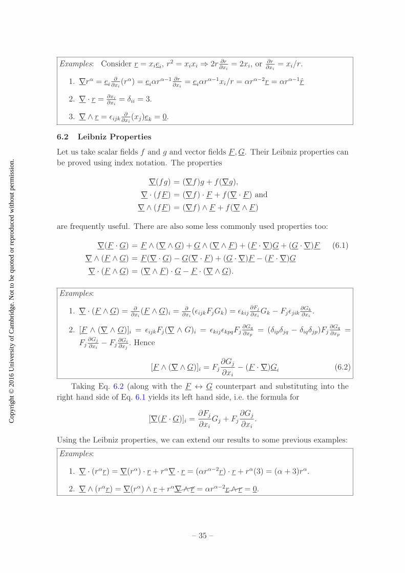
6.2 Leibniz Properties
Let us take scalar fields f and g and vector fields F ,G. Their Leibniz properties can
be proved using index notation. The properties
∇(fg) = (∇f)g + f(∇g),∇ · (fF ) = (∇f) · F + f(∇ · F ) and∇∧ (fF ) = (∇f) ∧ F + f(∇∧ F )
are frequently useful. There are also some less commonly used properties too:
∇(F ·G) = F ∧ (∇∧G) +G ∧ (∇∧ F ) + (F · ∇)G+ (G · ∇)F (6.1)
∇∧ (F ∧G) = F (∇ ·G)−G(∇ · F ) + (G · ∇)F − (F · ∇)G∇ · (F ∧G) = (∇∧ F ) ·G− F · (∇∧G).
Examples:
1. ∇ · (F ∧G) = ∂∂xi
(F ∧G)i = ∂∂xi
(ǫijkFjGk) = ǫkij∂Fj
∂xiGk − Fjǫjik ∂Gk
∂xi.
2. [F ∧ (∇ ∧ G)]i = ǫijkFj(∇ ∧ G)i = ǫkijǫkpqFj∂Gq
∂xp= (δipδjq − δiqδjp)Fj
∂Gq
∂xp=
Fj∂Gj
∂xi− Fj ∂Gi
∂xj. Hence
[F ∧ (∇∧G)]i = Fj∂Gj
∂xi− (F · ∇)Gi (6.2)
Taking Eq. 6.2 (along with the F ↔ G counterpart and substituting into the
right hand side of Eq. 6.1 yields its left hand side, i.e. the formula for
[∇(F ·G)]i =∂Fj∂xi
Gj + Fj∂Gj
∂xi.
Using the Leibniz properties, we can extend our results to some previous examples:
Examples:
1. ∇ · (rαr) = ∇(rα) · r + rα∇ · r = (αrα−2r) · r + rα(3) = (α + 3)rα.
2. ∇∧ (rαr) = ∇(rα) ∧ r + rα����∇∧ r = αrα−2���r ∧ r = 0.
– 35 –

Cop
yrig
ht ©
201
6 U
nive
rsity
of C
ambr
idge
. Not
to b
e qu
oted
or
repr
oduc
ed w
ithou
t per
mis
sion
.
6.3 Second Order Derivatives
If F = ∇, the field is called conservative. If ∇∧F = 0, a field is called or irrotational.
Two different combinations of grad, div and curl vanish identically: for any scalar
field f , ∇ ∧ (∇f) = 0 and for any vector field A, ∇ · (∇ ∧ A) = 0. Both of these
results follow from the symmetry of mixed partial derivatives:
ǫkij∂2f
∂xi∂xj= 0, ǫkij
∂2Ak∂xi∂xj
= 0.
The converse of each result also holds for fields defined on all of ℜ3:
∇∧ F = 0⇔ F = ∇f
for some f , a scalar potential. Also, again for H defined on1 ℜ3,
∇ ·H = 0⇔ H = ∇∧ A,
for some vector potential A. In this case, H is called solenoidal.
If F or H are defined only on subsets of ℜ3, then f or A may be defined only on
smaller subsets (see later).
The Laplacian operator is defined by
∇2 = ∇ · ∇ =∂2
∂xi∂xior (
∂2
∂x2+
∂2
∂y2+
∂2
∂z2).
On a scalar field, ∇2f = ∇ · (∇f) whereas on a vector field,
∇2A = ∇(∇ · A)−∇ ∧ (∇∧ A).
Again, this may be checked by using components.
7 Integral Theorems
The following closely-related results generalise the Fundamental Theorem of calculus:
that integration is the inverse of differentiation. To generalise to higher dimensions,
we need the right kind of derivative to match the right kind of integral.
7.1 Statements and Examples
7.1.1 Green’s theorem (in the plane)
For smooth functions P (x, y) and Q(x, y):
∫
A
(∂Q
∂x− ∂P
∂y) dA =
∫
C
(P dx+Q dy),
1We shall see in section 8.2 how this can change for a field which is not defined on all of ℜ3.
– 36 –
Cop
yrig
ht ©
201
6 U
nive
rsity
of C
ambr
idge
. Not
to b
e qu
oted
or
repr
oduc
ed w
ithou
t per
mis
sion
.
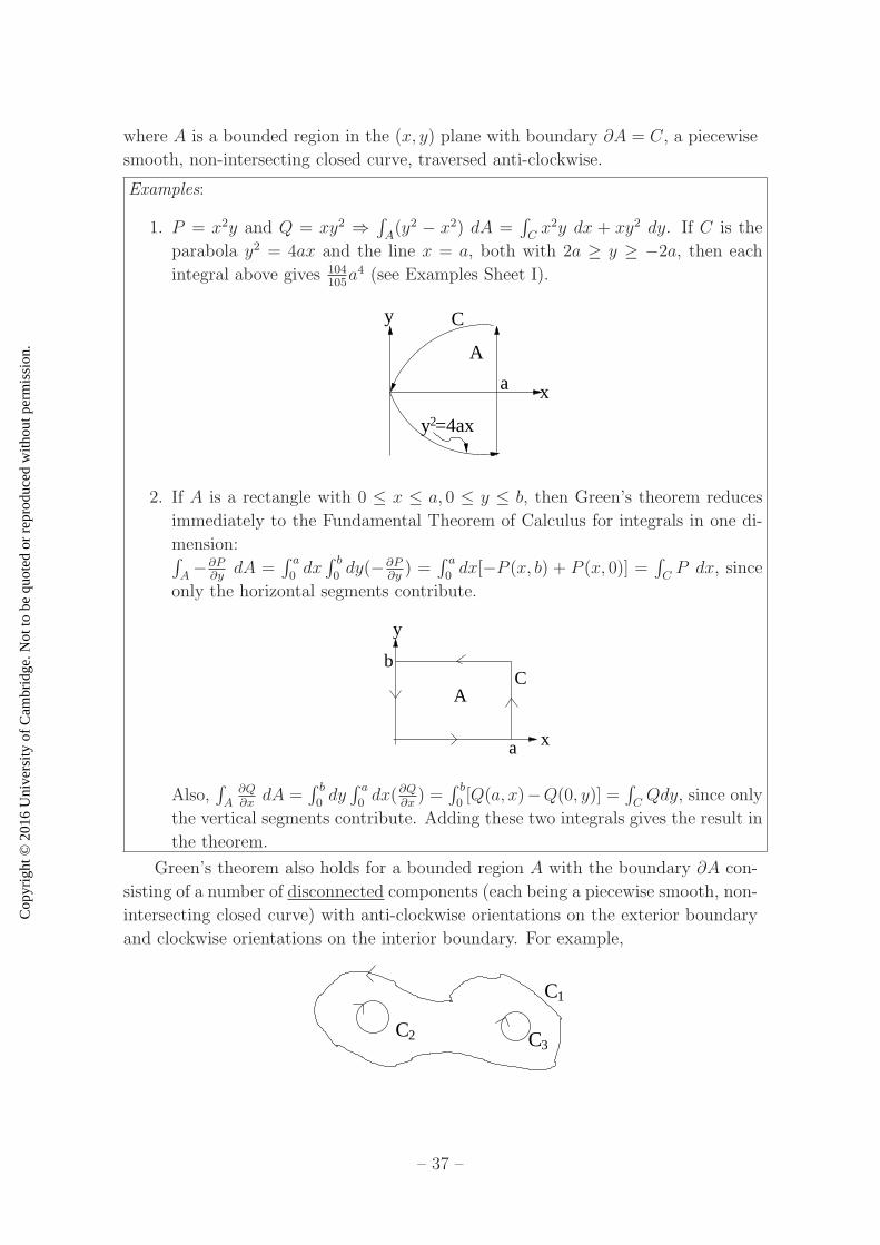
where A is a bounded region in the (x, y) plane with boundary ∂A = C, a piecewise
smooth, non-intersecting closed curve, traversed anti-clockwise.
Examples:
1. P = x2y and Q = xy2 ⇒∫
A(y2 − x2) dA =
∫
Cx2y dx + xy2 dy. If C is the
parabola y2 = 4ax and the line x = a, both with 2a ≥ y ≥ −2a, then each
integral above gives 104105a4 (see Examples Sheet I).
y
xa
C
A
y =4ax2
2. If A is a rectangle with 0 ≤ x ≤ a, 0 ≤ y ≤ b, then Green’s theorem reduces
immediately to the Fundamental Theorem of Calculus for integrals in one di-
mension:∫
A−∂P
∂ydA =
∫ a
0dx∫ b
0dy(−∂P
∂y) =
∫ a
0dx[−P (x, b) + P (x, 0)] =
∫
CP dx, since
only the horizontal segments contribute.
x
y
AC
a
b
Also,∫
A∂Q∂x
dA =∫ b
0dy∫ a
0dx(∂Q
∂x) =
∫ b
0[Q(a, x)−Q(0, y)] =
∫
CQdy, since only
the vertical segments contribute. Adding these two integrals gives the result in
the theorem.
Green’s theorem also holds for a bounded region A with the boundary ∂A con-
sisting of a number of disconnected components (each being a piecewise smooth, non-
intersecting closed curve) with anti-clockwise orientations on the exterior boundary
and clockwise orientations on the interior boundary. For example,
C C
C
2
1
3
– 37 –

Cop
yrig
ht ©
201
6 U
nive
rsity
of C
ambr
idge
. Not
to b
e qu
oted
or
repr
oduc
ed w
ithou
t per
mis
sion
.
These can be related to the case of a single boundary component using the construc-
tion from section 2.3:
since the horizontal parts cancel in the opposite directions (in the limit that they are
brought close together).
7.1.2 Stokes’ theorem
For a smooth vector field F (r):
∫
S
∇∧ F · dS =
∫
C
F · dr,
where S is a bounded smooth surface with boundary ∂S = C, a piecewise smooth
curve, and where S and C have compatible orientations. In detail: n is normal to S
(dS = n dS), t is tangent to C (dr = t ds). t and n have compatible orientations if
t ∧ n points out of S. Alternatively, moving around C in direction t with n ‘up’ ⇒that S is on the left.
C
tt
n
n
S
The theorem also holds if ∂S consists of a number of disconnected piecewise
smooth closed curves, with the same rule determining the orientation on each com-
ponent.
– 38 –
Cop
yrig
ht ©
201
6 U
nive
rsity
of C
ambr
idge
. Not
to b
e qu
oted
or
repr
oduc
ed w
ithou
t per
mis
sion
.
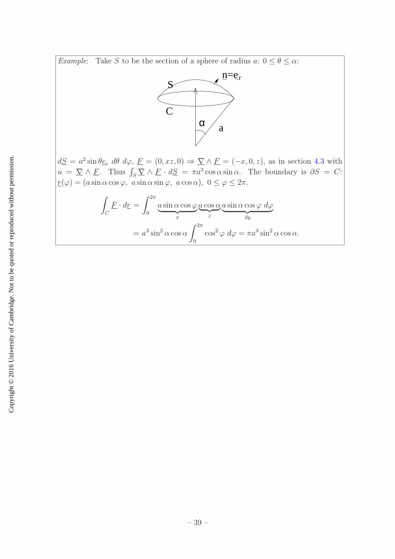
Example: Take S to be the section of a sphere of radius a: 0 ≤ θ ≤ α:
α a
C
Sn=er
dS = a2 sin θer dθ dϕ, F = (0, xz, 0) ⇒ ∇ ∧ F = (−x, 0, z), as in section 4.3 with
u = ∇ ∧ F . Thus∫
S∇ ∧ F · dS = πa3 cosα sinα. The boundary is ∂S = C:
r(ϕ) = (a sinα cosϕ, a sinα sinϕ, a cosα), 0 ≤ ϕ ≤ 2π.
∫
C
F · dr =
∫ 2π
0
a sinα cosϕ︸ ︷︷ ︸
x
a cosα︸ ︷︷ ︸
z
a sinα cosϕ dϕ︸ ︷︷ ︸
dy
= a3 sin2 α cosα
∫ 2π
0
cos2 ϕ dϕ = πa3 sin2 α cosα.
– 39 –
Cop
yrig
ht ©
201
6 U
nive
rsity
of C
ambr
idge
. Not
to b
e qu
oted
or
repr
oduc
ed w
ithou
t per
mis
sion
.
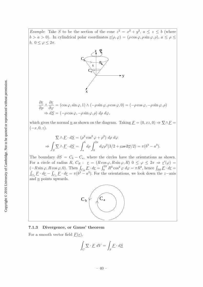
Example: Take S to be the section of the cone z2 = x2 + y2, a ≤ z ≤ b (where
b > a > 0). In cylindrical polar coordinates r(ρ, ϕ) = (ρ cosϕ, ρ sinϕ, ρ), a ≤ ρ ≤b, 0 ≤ ϕ ≤ 2π.
x
y
z
C
Cn
φ
S
a
b
∂r
∂ρ∧ ∂r
∂ϕ= (cosϕ, sinϕ, 1) ∧ (−ρ sinϕ, ρ cosϕ, 0) = (−ρ cosϕ,−ρ sinϕ, ρ)
⇒ dS = (−ρ cosϕ,−ρ sinϕ, ρ) dρ dϕ,
which gives the normal n as shown on the diagram. Taking F = (0, xz, 0)⇒ ∇∧F =
(−x, 0, z).
∇∧ F · dS = (ρ2 cos2 ϕ+ ρ2) dρ dϕ
⇒∫
S
∇∧ F · dS =
∫ b
a
dρ
∫ 2π
0
dϕρ2(3/2 +����cos 2ϕ/2) = π(b3 − a3).
The boundary ∂S = Cb − Ca, where the circles have the orientations as shown.
For a circle of radius R, CR : r = (R cosϕ,R sinϕ,R) 0 ≤ ϕ ≤ 2π ⇒ r′(ϕ) =
(−R sinϕ,R cosϕ, 0). Then∫
CRF · dr =
∫ 2π
0R3 cos2 ϕ dϕ = πR3, hence
∫
∂SF · dr =
∫
CbF · dr −
∫
CaF · dr = π(b3 − a3). For the orientations, we look down the z−axis
and n points upwards.
C Cb a
7.1.3 Divergence, or Gauss’ theorem
For a smooth vector field F (r),
∫
C
∇ · F dV =
∫
S
F · dS
– 40 –

Cop
yrig
ht ©
201
6 U
nive
rsity
of C
ambr
idge
. Not
to b
e qu
oted
or
repr
oduc
ed w
ithou
t per
mis
sion
.
where V is a bounded volume with boundary ∂V = S, a piecewise smooth closed
surface with normal n pointing outwards.
Example: Take V to be the solid hemisphere x2 + y2 + z2 ≤ a2, z ≥ 0. ∂V = S =
S1(hemisphere) + S2(disc).
n
n
S
S1
2
F = (0, 0, z + a) ⇒ ∇ · F = 1. Then,∫
V∇ · F dV = 2/3πa3, the volume of the
hemisphere.
On S1: dS = n dS = (x, y, z)/a dS.
F · dS = z(z + a)/a dS = a cos θ(cos θ + 1)a2 sin θ dθ dϕ.
⇒∫
S1
F · dS =
∫ 2π
0
dϕa3∫ π/2
0
dθ sin θ(cos2 θ + cos θ)
= 2πa3[
−1
3cos3 θ − 1
2cos2 θ
]π/2
0
=5
3πa3.
On S2 : dS = n dS = −(0, 0, 1) dS. F · dS = −a dS and so∫
S2F · dS = −πa3.
Hence∫
S1F · dS +
∫
S2F · dS = 5/3πa3− πa3 = 2/3πa3, agreeing with the prediction
of the theorem.
7.2 Relating and Proving the Integral Theorems
7.2.1 Proving Green’s theorem from Stokes’ theorem or the 2d diver-
gence theorem
Let A be a region in the (x, y) plane with boundary C = ∂A parameterised by arc
length, with the sense shown: (x(s), y(s), 0):
C
t
n
k
t = (dx/ds, dy/ds, 0) is the unit tangent to C and n = (dy/ds,−dx/ds, 0) is the unitnormal to C out of A. n = t ∧ k, where k = (0, 0, 1).
– 41 –
Cop
yrig
ht ©
201
6 U
nive
rsity
of C
ambr
idge
. Not
to b
e qu
oted
or
repr
oduc
ed w
ithou
t per
mis
sion
.
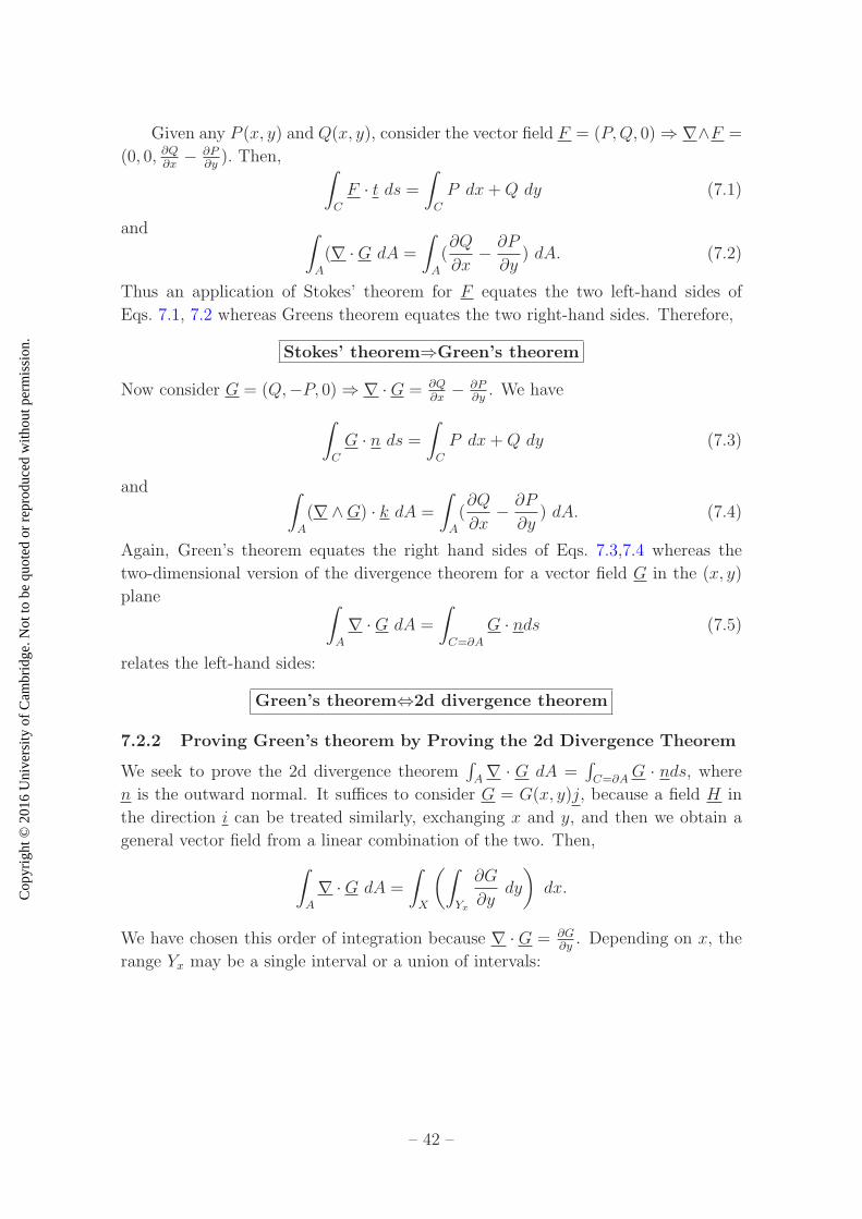
Given any P (x, y) and Q(x, y), consider the vector field F = (P,Q, 0)⇒ ∇∧F =
(0, 0, ∂Q∂x− ∂P
∂y). Then,
∫
C
F · t ds =∫
C
P dx+Q dy (7.1)
and ∫
A
(∇ ·G dA =
∫
A
(∂Q
∂x− ∂P
∂y) dA. (7.2)
Thus an application of Stokes’ theorem for F equates the two left-hand sides of
Eqs. 7.1, 7.2 whereas Greens theorem equates the two right-hand sides. Therefore,
Stokes’ theorem⇒Green’s theorem
Now consider G = (Q,−P, 0)⇒ ∇ ·G = ∂Q∂x− ∂P
∂y. We have
∫
C
G · n ds =∫
C
P dx+Q dy (7.3)
and ∫
A
(∇∧G) · k dA =
∫
A
(∂Q
∂x− ∂P
∂y) dA. (7.4)
Again, Green’s theorem equates the right hand sides of Eqs. 7.3,7.4 whereas the
two-dimensional version of the divergence theorem for a vector field G in the (x, y)
plane ∫
A
∇ ·G dA =
∫
C=∂A
G · nds (7.5)
relates the left-hand sides:
Green’s theorem⇔2d divergence theorem
7.2.2 Proving Green’s theorem by Proving the 2d Divergence Theorem
We seek to prove the 2d divergence theorem∫
A∇ · G dA =
∫
C=∂AG · nds, where
n is the outward normal. It suffices to consider G = G(x, y)j, because a field H in
the direction i can be treated similarly, exchanging x and y, and then we obtain a
general vector field from a linear combination of the two. Then,
∫
A
∇ ·G dA =
∫
X
(∫
Yx
∂G
∂ydy
)
dx.
We have chosen this order of integration because ∇ · G = ∂G∂y. Depending on x, the
range Yx may be a single interval or a union of intervals:
– 42 –
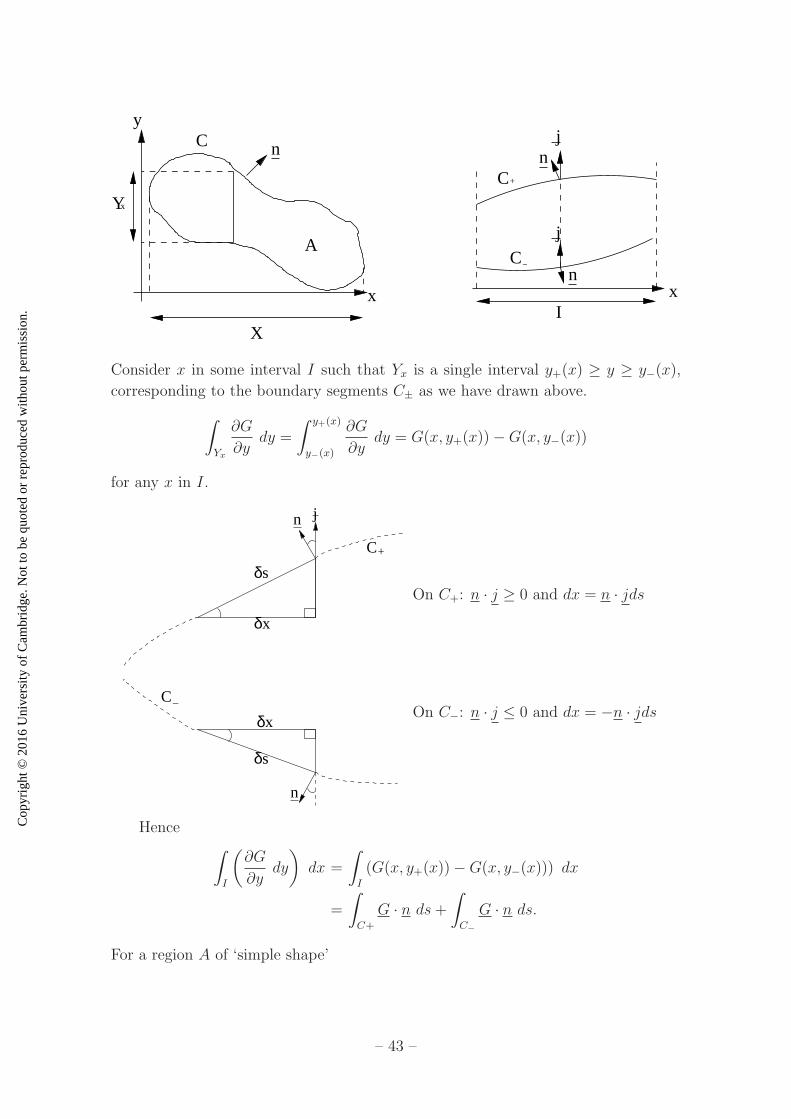
Cop
yrig
ht ©
201
6 U
nive
rsity
of C
ambr
idge
. Not
to b
e qu
oted
or
repr
oduc
ed w
ithou
t per
mis
sion
.
Y
X
A
C n
x
yj
j
n
n
C
C
xI
x
+
−
Consider x in some interval I such that Yx is a single interval y+(x) ≥ y ≥ y−(x),
corresponding to the boundary segments C± as we have drawn above.
∫
Yx
∂G
∂ydy =
∫ y+(x)
y−(x)
∂G
∂ydy = G(x, y+(x))−G(x, y−(x))
for any x in I.
C
xδ
sδ
n
−
jn
s
x
δ
δ
C+
On C+: n · j ≥ 0 and dx = n · jds
On C−: n · j ≤ 0 and dx = −n · jds
Hence∫
I
(∂G
∂ydy
)
dx =
∫
I
(G(x, y+(x))−G(x, y−(x))) dx
=
∫
C+
G · n ds+∫
C−
G · n ds.
For a region A of ‘simple shape’
– 43 –

Cop
yrig
ht ©
201
6 U
nive
rsity
of C
ambr
idge
. Not
to b
e qu
oted
or
repr
oduc
ed w
ithou
t per
mis
sion
.
x
y
A
C
C
X
+
−
as shown, we take I = X and ∂A = C+ + C− and the integrals over C± combine to
give∫
CG · n ds, proving the result.
For regions A of more general shape, either:
1. Divide A into simpler subsets which do have the property above. The result
holds on each subset Ai ⇒ it holds on A
A
A
AA
A
1
2
3
4
5
2. Proceed directly, even if Yx is a sum of intervals and get a sum over all boundary
segments corresponding to x in the range I
I
C
C
C
1
2
3
∫
I
(∫
Yx
∂G
∂ydy
)
dx =∑
i
∫
Ci
G · n ds.
– 44 –
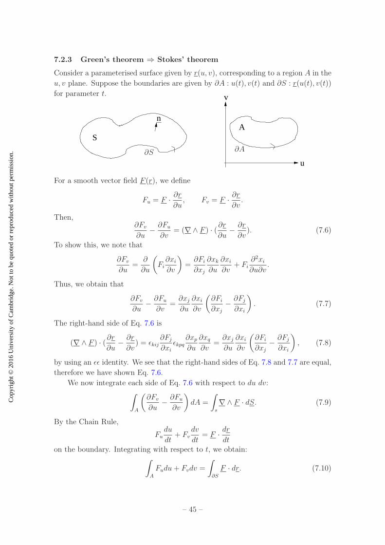
Cop
yrig
ht ©
201
6 U
nive
rsity
of C
ambr
idge
. Not
to b
e qu
oted
or
repr
oduc
ed w
ithou
t per
mis
sion
.
7.2.3 Green’s theorem ⇒ Stokes’ theorem
Consider a parameterised surface given by r(u, v), corresponding to a region A in the
u, v plane. Suppose the boundaries are given by ∂A : u(t), v(t) and ∂S : r(u(t), v(t))
for parameter t.
S
n
u
v
A
∂S ∂A
For a smooth vector field F (r), we define
Fu = F · ∂r∂u, Fv = F · ∂r
∂v.
Then,∂Fv∂u− ∂Fu
∂v= (∇∧ F ) · (∂r
∂u− ∂r
∂v). (7.6)
To show this, we note that
∂Fv∂u
=∂
∂u
(
Fi∂xi∂v
)
=∂Fi∂xj
∂xk∂u
∂xi∂v
+ Fi∂2xi∂u∂v
.
Thus, we obtain that
∂Fv∂u− ∂Fu
∂v=∂xj∂u
∂xi∂v
(∂Fi∂xj− ∂Fj∂xi
)
. (7.7)
The right-hand side of Eq. 7.6 is
(∇∧ F ) · (∂r∂u− ∂r
∂v) = ǫkij
∂Fj∂xi
ǫkpq∂xp∂u
∂xq∂v
=∂xj∂u
∂xi∂v
(∂Fi∂xj− ∂Fj∂xi
)
, (7.8)
by using an ǫǫ identity. We see that the right-hand sides of Eq. 7.8 and 7.7 are equal,
therefore we have shown Eq. 7.6.
We now integrate each side of Eq. 7.6 with respect to du dv:∫
A
(∂Fv∂u− ∂Fu
∂v
)
dA =
∫
s
∇∧ F · dS. (7.9)
By the Chain Rule,
Fudu
dt+ Fv
dv
dt= F · dr
dton the boundary. Integrating with respect to t, we obtain:
∫
A
Fudu+ Fvdv =
∫
∂S
F · dr. (7.10)
– 45 –
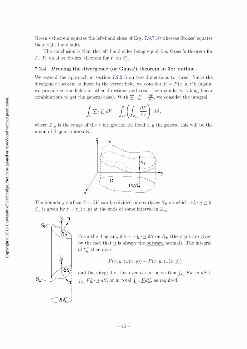
Cop
yrig
ht ©
201
6 U
nive
rsity
of C
ambr
idge
. Not
to b
e qu
oted
or
repr
oduc
ed w
ithou
t per
mis
sion
.
Green’s theorem equates the left-hand sides of Eqs. 7.9,7.10 whereas Stokes’ equates
their right-hand sides.
The conclusion is that the left hand sides being equal (i.e. Green’s theorem for
Fi, Fv on A ⇔ Stokes’ theorem for F on S).
7.2.4 Proving the divergence (or Gauss’) theorem in 3d: outline
We extend the approach in section 7.2.2 from two dimensions to three. Since the
divergence theorem is linear in the vector field, we consider F = F (x, y, z)k (again,
we provide vector fields in other directions and treat them similarly, taking linear
combinations to get the general case). With ∇ · F = ∂F∂z, we consider the integral
∫
V
∇ · F dV =
∫
D
(∫
Zxy
∂F
∂z
)
dA,
where Zxy is the range of the z integration for fixed x, y (in general this will be the
union of disjoint intervals).
D(x,y)
z
x
y
zxy
V
The boundary surface S = ∂V can be divided into surfaces S± on which ±k · n ≥ 0.
S± is given by z = z±(x, y) at the ends of some interval in Zxy.
k n
k
n
A
S
S
S
S
δ
δ
δ
+
−
From the diagram, δA = ±k · n δS on S± (the signs are given
by the fact that n is always the outward normal). The integral
of ∂F∂z
then gives
F (x, y, z+(x, y))− F (x, y, z−(x, y))
and the integral of this over D can be written∫
S+Fk · n dS +
∫
S−
Fk · n dS, or in total∫
∂VF dS, as required.
– 46 –

Cop
yrig
ht ©
201
6 U
nive
rsity
of C
ambr
idge
. Not
to b
e qu
oted
or
repr
oduc
ed w
ithou
t per
mis
sion
.
8 Some Applications of Integral Theorems
8.1 Integral Expressions of Div and Curl
The divergence theorem for a vector field F applied to a small volume V containing
a point r0 gives ∫
∂V
F · dS =
∫
V
∇ · F dV ≈ (∇ · F )(r0)V.
F
r 0
This becomes exact on taking the limit at r0:
∇ · F = limV→01V
∫
∂VF · dS.
Similarly, Stokes’ theorem applied to a small part of a plane with area A and normal
n gives ∫
∂A
F · dr =∫
A
(∇∧ F ) · n dA ≈ (n · ∇ ∧ F )(r0)A.
F
n
A ro
At r0,
n · ∇ ∧ F = limA→01A
∫
∂AF · dr.
These are manifestly coordinate independent definitions of div and curl.
– 47 –

Cop
yrig
ht ©
201
6 U
nive
rsity
of C
ambr
idge
. Not
to b
e qu
oted
or
repr
oduc
ed w
ithou
t per
mis
sion
.
Examples: The expressions above allow interpretations of ∇ · u and ∇∧ u when u is
a velocity field, describing fluid flow.
1. Divergence: we know from section 4.3 that∫
Su ·dS is the rate of fluid crossing
δS (i.e. per unit time). Taking V to be the volume occupied by a fixed material
quantity of fluid, we therefore have V =∫
∂Su · dS (for a boundary ∂V at some
fixed time interval, δtV is the approximate volume that crosses in time δt,
as the volume occupied by the fixed material quantity changes). Then, from
above, at r0, ∇ · u = limV→0V /V , the local (i.e. at r0) relative rate of change
of volume occupied by a fixed material quantity of fluid.
For example, u(r) = αr, fluid flows out of the origin. ∇ · u = 3α, i.e. the
volume increases at the same constant relative rate everywhere.
2. Curl: Take the plane area A to be a disc of radius a.
n
ut
∫
∂Au · dr =
∫
∂Au · t ds = (2πa)× the average of u · t, the component tangential
to the boundary = 2πa2ω, where we define ω = 1/a× (the average of u · t), asthe local angular velocity around n. Then
n · ∇ ∧ u = lima→01
πa2(2πa2ω) = 2ω
at r0, i.e. twice the local rate of rotation. For example, u = ω∧ r, rigid motion
with constant angular velocity ω about 0, and ∇∧ (ω∧ r) = 2ω, twice the rate
of rotation.
8.2 Conservative and Irrotational Fields, and Scalar Potentials
Consider three ways to define a vector field F , (A) and (B) are equivalent definitions
of a conservative vector field, and (C) defines an irrotational field:
(A) F = ∇f for some scalar field f(r).
(B)∫
CF · dr is independent of C, for some given end points and orienta-
tion.
(C) ∇∧ F = 0.
(A), (B) and (C) are all equivalent for F (r) on ℜ3. (A)⇒(B) with∫
CF ·dr = f(b)−
f(a) was shown in section 2.4. (A)⇒(C) was shown in section 6.3 (via ∇∧∇f = 0.)
We shall now show that (C)⇒(B) and (B)⇒(A) in ℜ3. Given F (r) obeying (C)
on ℜ3, let C and C be any two curves from a→ b:
– 48 –
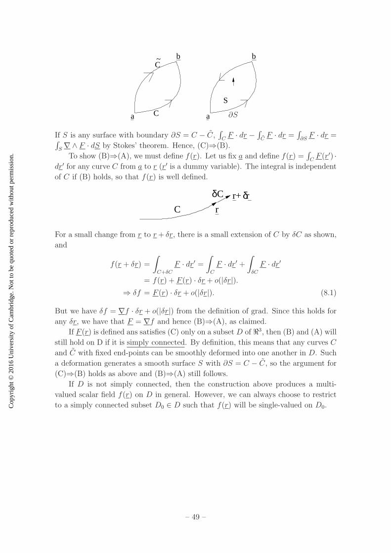
Cop
yrig
ht ©
201
6 U
nive
rsity
of C
ambr
idge
. Not
to b
e qu
oted
or
repr
oduc
ed w
ithou
t per
mis
sion
.
a
b
a
b
S
C
C~
∂S
If S is any surface with boundary ∂S = C − C,∫
CF · dr −
∫
CF · dr =
∫
∂SF · dr =
∫
S∇∧ F · dS by Stokes’ theorem. Hence, (C)⇒(B).
To show (B)⇒(A), we must define f(r). Let us fix a and define f(r) =∫
CF (r′) ·
dr′ for any curve C from a to r (r′ is a dummy variable). The integral is independent
of C if (B) holds, so that f(r) is well defined.
C r
r+ rδCδ
For a small change from r to r+ δr, there is a small extension of C by δC as shown,
and
f(r + δr) =
∫
C+δC
F · dr′ =∫
C
F · dr′ +∫
δC
F · dr′
= f(r) + F (r) · δr + o(|δr|).⇒ δf = F (r) · δr + o(|δr|). (8.1)
But we have δf = ∇f · δr + o(|δr|) from the definition of grad. Since this holds for
any δr, we have that F = ∇f and hence (B)⇒(A), as claimed.
If F (r) is defined ans satisfies (C) only on a subset D of ℜ3, then (B) and (A) will
still hold on D if it is simply connected. By definition, this means that any curves C
and C with fixed end-points can be smoothly deformed into one another in D. Such
a deformation generates a smooth surface S with ∂S = C − C, so the argument for
(C)⇒(B) holds as above and (B)⇒(A) still follows.
If D is not simply connected, then the construction above produces a multi-
valued scalar field f(r) on D in general. However, we can always choose to restrict
to a simply connected subset D0 ∈ D such that f(r) will be single-valued on D0.
– 49 –

Cop
yrig
ht ©
201
6 U
nive
rsity
of C
ambr
idge
. Not
to b
e qu
oted
or
repr
oduc
ed w
ithou
t per
mis
sion
.
Example: F = (−y/(x2 + y2), x/(x2 + y2), 0) is well-defined and obeys ∇∧F = 0 on
D = ℜ3 − {z-axis}, which is not simply connected.
C
C
~
usual polarangle
φ,
F = ∇f where f = tan−1(y/x) = ϕ is multi-valued on D, but single-valued on
D0 = ℜ3 − {half plane x ≥ 0, y = 0}, in other words simply connected on D0.
8.3 Conservation Laws
Consider time-dependent scalar and vector fields ρ(r, t) and j(r, t) obeying the conservation equation
∂ρ
∂t+∇ · j = 0.
Let V be a fixed t−independent volume with boundary S = ∂V . Then Q(t) =∫
Vρ(r, t) dV satisfies
dQ
dt=
∫
V
∂ρ
∂tdV = −
∫
V
∇ · j dV = −∫
S
j · dS
by the divergence theorem at fixed t.
Q(t)
V
j
n
Q(t) is the total amount of some quantity in V ; ρ(r, t) is the density for this quantity,
with ρ(r, t)δV the amount in a small volume δV ; the flux of j out of S gives the rate
of quantity leaving V , according to the equation above.
– 50 –
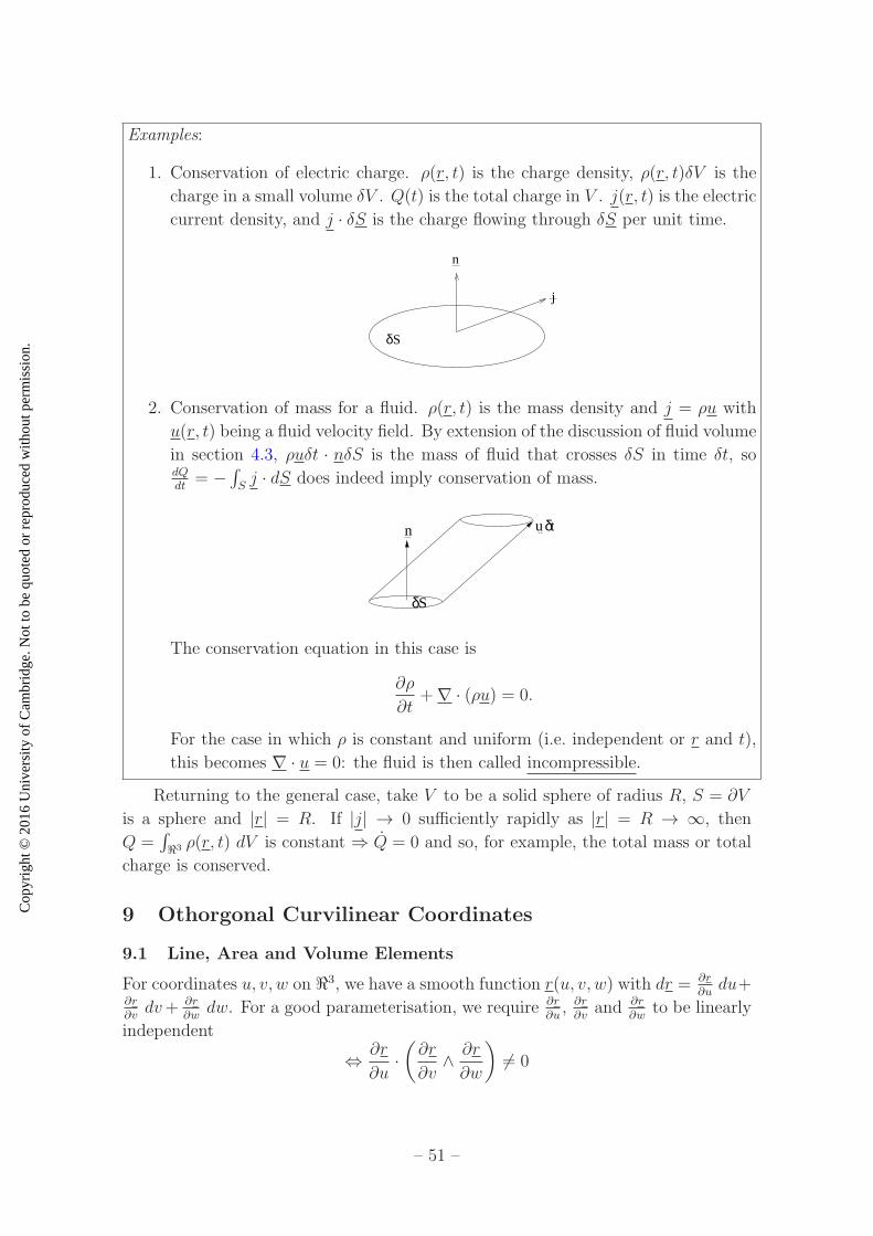
Cop
yrig
ht ©
201
6 U
nive
rsity
of C
ambr
idge
. Not
to b
e qu
oted
or
repr
oduc
ed w
ithou
t per
mis
sion
.
Examples:
1. Conservation of electric charge. ρ(r, t) is the charge density, ρ(r, t)δV is the
charge in a small volume δV . Q(t) is the total charge in V . j(r, t) is the electric
current density, and j · δS is the charge flowing through δS per unit time.
j
n
Sδ
2. Conservation of mass for a fluid. ρ(r, t) is the mass density and j = ρu with
u(r, t) being a fluid velocity field. By extension of the discussion of fluid volume
in section 4.3, ρuδt · nδS is the mass of fluid that crosses δS in time δt, sodQdt
= −∫
Sj · dS does indeed imply conservation of mass.
n u t
S
δ
δ
The conservation equation in this case is
∂ρ
∂t+∇ · (ρu) = 0.
For the case in which ρ is constant and uniform (i.e. independent or r and t),
this becomes ∇ · u = 0: the fluid is then called incompressible.
Returning to the general case, take V to be a solid sphere of radius R, S = ∂V
is a sphere and |r| = R. If |j| → 0 sufficiently rapidly as |r| = R → ∞, then
Q =∫
ℜ3 ρ(r, t) dV is constant ⇒ Q = 0 and so, for example, the total mass or total
charge is conserved.
9 Othorgonal Curvilinear Coordinates
9.1 Line, Area and Volume Elements
For coordinates u, v, w on ℜ3, we have a smooth function r(u, v, w) with dr = ∂r∂udu+
∂r∂vdv+ ∂r
∂wdw. For a good parameterisation, we require ∂r
∂u, ∂r∂v
and ∂r∂w
to be linearly
independent
⇔ ∂r
∂u·(∂r
∂v∧ ∂r
∂w
)
6= 0
– 51 –

Cop
yrig
ht ©
201
6 U
nive
rsity
of C
ambr
idge
. Not
to b
e qu
oted
or
repr
oduc
ed w
ithou
t per
mis
sion
.
(see the Jacobian condition in section 4.4.2). These vectors are tangent to the curves
parameterised by u, v and w when the other two are held fixed.
We say that u, v, w are orthogonal curvilinear coodinates if the tangent vectors
above are orthogonal. Then, we can set ∂r∂u
= hueu,∂r∂v
= hvev,∂r∂w
= hwew, with
hu > 0, hv > 0, hw > 0 and eu, ev, ew forming an orthonormal and right-handed
basis (right-handed meaning eu ∧ ev = ew, which may be achieved by ordering the
coordinates appropriately). In these coordinates, the line element is
dr = hueu du+ hvev dv + hwew dw
and the positive scale factors hu, hv, hw determine the changes in length along each
orthogonal direction resulting from changes in u, v and w:
|δr|2 = h2u(δu)2 + h2v(δv)
2 + h2w(δw)2 + o-terms
Examples:
1. Cartesian coordinates r(x, y, z) = xi + yj + zk. hx = hy = hz = 1, ex = i,
ey = j, ez = k.
2. Cylindrical polar coordinates r(ρ, ϕ, z) = ρ(cosϕi + sinϕj) + zk, hρ = hz =
1, hϕ = ρ. eρ, eϕ and ez are as in section 1.3.
3. Spherical polar coordinates r(r, θ, ϕ) = r(cosϕ sin θi + sinϕ sin θj + cos θk),
hr = 1, hθ = r, hϕ = r sin θ. er, eθ, eϕ are as in section 1.3.
Consider a surface with w constant (say), parameterised by u and v. The vector
area element is dS = ∂r∂u∧ ∂r
∂vdu dv (a general formula) = hueu ∧ hvev du dv =
huhvew du dv, for orthogonal coordinates.
e
ee
u
vw
ew is normal to the surface and we can see that δS is a small rectangle with sides
huδu and hvδv, approximately. The volume element dV = ∂r∂u·(∂r∂v∧ ∂r
∂w
)
du dv dw =
huhvhw du dv dw, which corresponds to a small cuboid with sides huδu, hvδv and
hwδw, approximately.
9.2 Grad, Div and Curl
Consider f(r(u, v, w)) and compare
df =∂f
∂udu+
∂f
∂vdv +
∂f
∂wdw
– 52 –
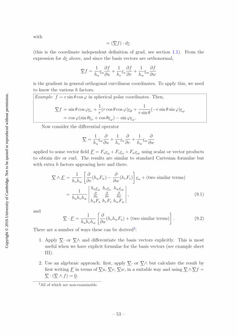
Cop
yrig
ht ©
201
6 U
nive
rsity
of C
ambr
idge
. Not
to b
e qu
oted
or
repr
oduc
ed w
ithou
t per
mis
sion
.
with
= (∇f) · dr.(this is the coordinate independent definition of grad, see section 1.1). From the
expression for dr above, and since the basis vectors are orthonormal,
∇f =1
hueu∂f
∂u+
1
hvev∂f
∂v+
1
hwew∂f
∂w
is the gradient in general orthogonal curvilinear coordinates. To apply this, we need
to know the various h factors.
Example: f = r sin θ cosϕ in spherical polar coordinates. Then,
∇f = sin θ cosϕer +1
r(r cos θ cosϕ)eθ +
1
r sin θ(−r sin θ sinϕ)eϕ
= cosϕ(sin θer + cos θeϕ)− sinϕeϕ.
Now consider the differential operator
∇ =1
hueu
∂
∂u+
1
hvev∂
∂v+
1
hwew
∂
∂w
applied to some vector field F = Fueu+Fvev +Fwew using scalar or vector products
to obtain div or curl. The results are similar to standard Cartesian formulae but
with extra h factors appearing here and there.
∇∧ F =1
hvhw
[∂
∂v(hwFw)−
∂
∂w(hvFv)
]
eu + (two similar terms)
=1
huhvhw
∣∣∣∣∣∣
hueu hvev hwew∂∂u
∂∂v
∂∂w
huFu hvFv hwFw
∣∣∣∣∣∣
, (9.1)
and
∇ · F =1
huhvhw
[∂
∂u(hvhwFu) + (two similar terms)
]
. (9.2)
There are a number of ways these can be derived2:
1. Apply ∇· or ∇∧ and differentiate the basis vectors explicitly. This is most
useful when we have explicit formulae for the basis vectors (see example sheet
III).
2. Use an algebraic approach: first, apply ∇· or ∇∧ but calculate the result by
first writing F in terms of ∇u, ∇v, ∇w, in a suitable way and using ∇∧∇f =
∇ · (∇∧ f) = 0.
2All of which are non-examinable.
– 53 –
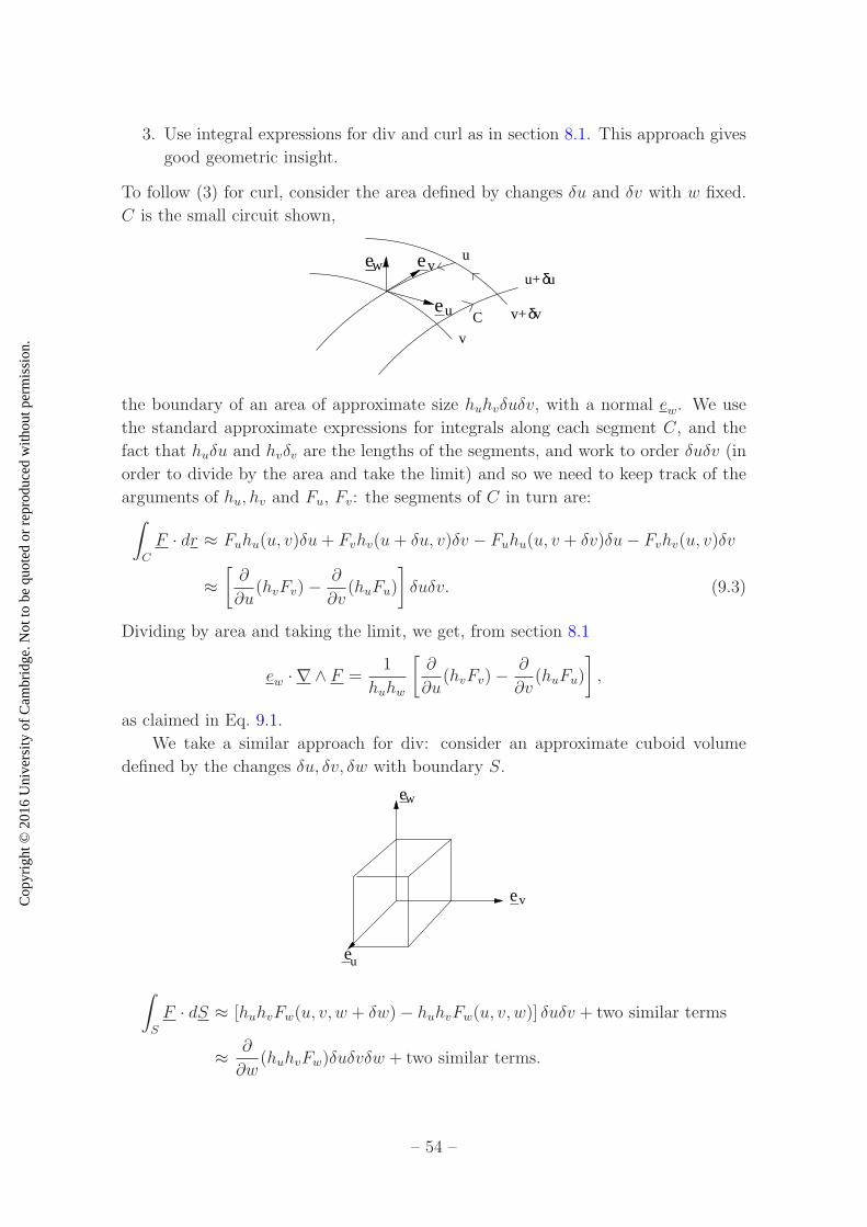
Cop
yrig
ht ©
201
6 U
nive
rsity
of C
ambr
idge
. Not
to b
e qu
oted
or
repr
oduc
ed w
ithou
t per
mis
sion
.
3. Use integral expressions for div and curl as in section 8.1. This approach gives
good geometric insight.
To follow (3) for curl, consider the area defined by changes δu and δv with w fixed.
C is the small circuit shown,
e
ee
u
vw
C
v
v+ v
u
u+ u
δ
δ
the boundary of an area of approximate size huhvδuδv, with a normal ew. We use
the standard approximate expressions for integrals along each segment C, and the
fact that huδu and hvδv are the lengths of the segments, and work to order δuδv (in
order to divide by the area and take the limit) and so we need to keep track of the
arguments of hu, hv and Fu, Fv: the segments of C in turn are:∫
C
F · dr ≈ Fuhu(u, v)δu+ Fvhv(u+ δu, v)δv − Fuhu(u, v + δv)δu− Fvhv(u, v)δv
≈[∂
∂u(hvFv)−
∂
∂v(huFu)
]
δuδv. (9.3)
Dividing by area and taking the limit, we get, from section 8.1
ew · ∇ ∧ F =1
huhw
[∂
∂u(hvFv)−
∂
∂v(huFu)
]
,
as claimed in Eq. 9.1.
We take a similar approach for div: consider an approximate cuboid volume
defined by the changes δu, δv, δw with boundary S.
e
eu
ev
w
∫
S
F · dS ≈ [huhvFw(u, v, w + δw)− huhvFw(u, v, w)] δuδv + two similar terms
≈ ∂
∂w(huhvFw)δuδvδw + two similar terms.
– 54 –
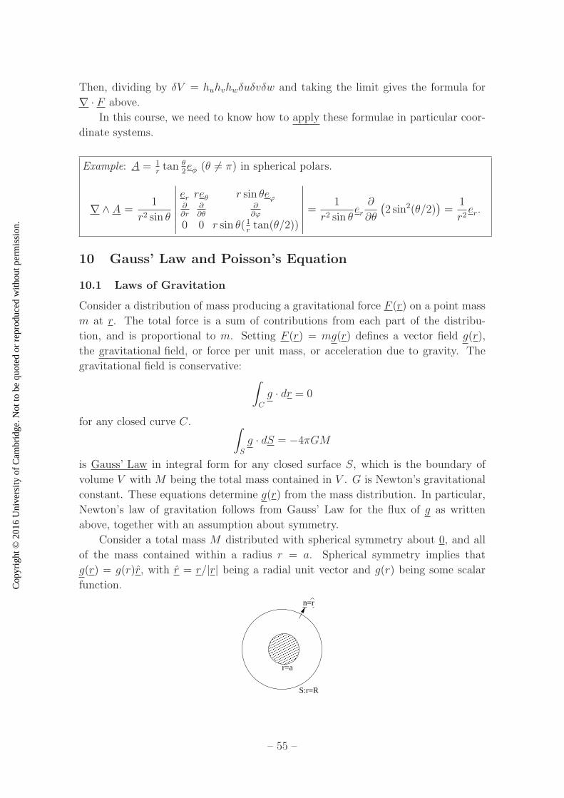
Cop
yrig
ht ©
201
6 U
nive
rsity
of C
ambr
idge
. Not
to b
e qu
oted
or
repr
oduc
ed w
ithou
t per
mis
sion
.
Then, dividing by δV = huhvhwδuδvδw and taking the limit gives the formula for
∇ · F above.
In this course, we need to know how to apply these formulae in particular coor-
dinate systems.
Example: A = 1rtan θ
2eφ (θ 6= π) in spherical polars.
∇∧ A =1
r2 sin θ
∣∣∣∣∣∣∣
er reθ r sin θeϕ∂∂r
∂∂θ
∂∂ϕ
0 0 r sin θ(1rtan(θ/2))
∣∣∣∣∣∣∣
=1
r2 sin θer∂
∂θ
(2 sin2(θ/2)
)=
1
r2er.
10 Gauss’ Law and Poisson’s Equation
10.1 Laws of Gravitation
Consider a distribution of mass producing a gravitational force F (r) on a point mass
m at r. The total force is a sum of contributions from each part of the distribu-
tion, and is proportional to m. Setting F (r) = mg(r) defines a vector field g(r),
the gravitational field, or force per unit mass, or acceleration due to gravity. The
gravitational field is conservative:∫
C
g · dr = 0
for any closed curve C. ∫
S
g · dS = −4πGM
is Gauss’ Law in integral form for any closed surface S, which is the boundary of
volume V with M being the total mass contained in V . G is Newton’s gravitational
constant. These equations determine g(r) from the mass distribution. In particular,
Newton’s law of gravitation follows from Gauss’ Law for the flux of g as written
above, together with an assumption about symmetry.
Consider a total mass M distributed with spherical symmetry about 0, and all
of the mass contained within a radius r = a. Spherical symmetry implies that
g(r) = g(r)r, with r = r/|r| being a radial unit vector and g(r) being some scalar
function.
�����������������������������������
�����������������������������������
n=r
S:r=R
r=a
– 55 –

Cop
yrig
ht ©
201
6 U
nive
rsity
of C
ambr
idge
. Not
to b
e qu
oted
or
repr
oduc
ed w
ithou
t per
mis
sion
.
Consider Gauss’ Law with S being a sphere of radius r = R > a. The outward
normal is r.
∫
S
g · dS =
∫
S
g(R)r · rdS =
∫
S
g(R)dS = 4πR2g(R)
by using spherical symmetry. Then, using Gauss’ Law,
4πR2g(R) = −4πGM ⇒ g(R) = −GMR2
for any R > a, or
g(r) = −GMr2
r (r > a).
The gravitational force on a mass m at r is therefore F (r) = −GMmr/r2. In
the limit a→ 0 we get a point mass M at the origin 0 and we recover Newton’s Law
of Gravitation for point masses.
For any a, the field and the force for r > a depends only on the total mass M ,
assuming spherical symmetry (and no mass in r > a). This simple behaviour means
that we can identify the gravitational field that keeps the moon in orbit (where the
earth is approximately point-like) with the one that pulls an apple from a tree (where
the earth is certainly not point-like).
The condition∫
Cg · dr = 0 for any closed C can be re-written
∫
S∇ ∧ gdS = 0
for any S with ∂S = C by Stokes’ theorem. Since S is arbitrary, this ⇔ ∇∧ g = 0.
In our above example with spherical symmetry, ∇∧ g = 0 automatically.
If the mass distribution is not sufficiently symmetrical, it is difficult to solve for
g(r) from Gauss’ Law in integral form, but it can be re-cast in differential form.
Suppose that the mass M arises from a mass density ρ(r). Then
∫
S
g · dS = −4πGM ⇒∫
V
∇ · gdV = −4πG∫
V
ρ(r) dV
with S = ∂V by Gauss’ theorem ⇒∫
V(∇ · g + 4πGρ) dV = 0 for any volume V ,
hence
⇒ ∇ · g = −4πGρ,Gauss’ law in differential form. Furthermore, since ∇∧ g = 0, we can introduce the
gravitational potential ϕ(r) with g = −∇ϕ and then Gauss’ law becomes
∇2ϕ = 4πGρ,
Poisson’s equation. In the previous case with spherical symmetry, we can choose
ϕ(r) = −GM/r for r > a. It obeys the boundary condition ϕ→ 0 as r →∞.
– 56 –

Cop
yrig
ht ©
201
6 U
nive
rsity
of C
ambr
idge
. Not
to b
e qu
oted
or
repr
oduc
ed w
ithou
t per
mis
sion
.
10.2 Laws of Electrostatics
Consider a distribution of electric charges at rest. They produce a force on a charge
a at rest at r which is proportional to q: F = qE(r), where E(r) is the electric field
(a vector field), or force per unit charge.
The electric field obeys∫
CE · dr = 0 for any closed curve C, i.e. E(r) is conser-
vative. Also, it obeys Gauss’ Law:
∫
S
E · dS =Q
ǫ0
for any closed surface S which is the boundary of a volume V , with Q being the total
charge contained within V . ǫ0 is the permittivity of free space, a constant of nature.
Mathematically speaking, this is identical to the gravitational case in section 10.1,
and the laws above can be re-expressed in differential form in the same way: ∇∧E = 0
and
∇ · E =ρ
ǫ0
(Gauss’ Law in differential form), where ρ(r) is the electric charge density. these
can be re-expressed as E = −∇ϕ, with ϕ(r) being the electrostatic potential and
∇2ϕ = −ρ/ǫ0, Poisson’s equation.For example: take a total charge Q distributed with spherical symmetry about
0 and all of the charge being contained within a radius r = a. We solve this using
Gauss’ Law in integral form, just as in the gravitational case. Thus,
E(r) =Q
4πǫ0
r
r2
for r > a and
ϕ(r) =Q
4πǫ0
1
r.
we obtain a point charge at 0 in the limit a→ 0. from this result for E, we recover
Coulomb’s Law for the force on another point charge q at r:
F = qE =qQ
4πǫ0
r
r2.
– 57 –
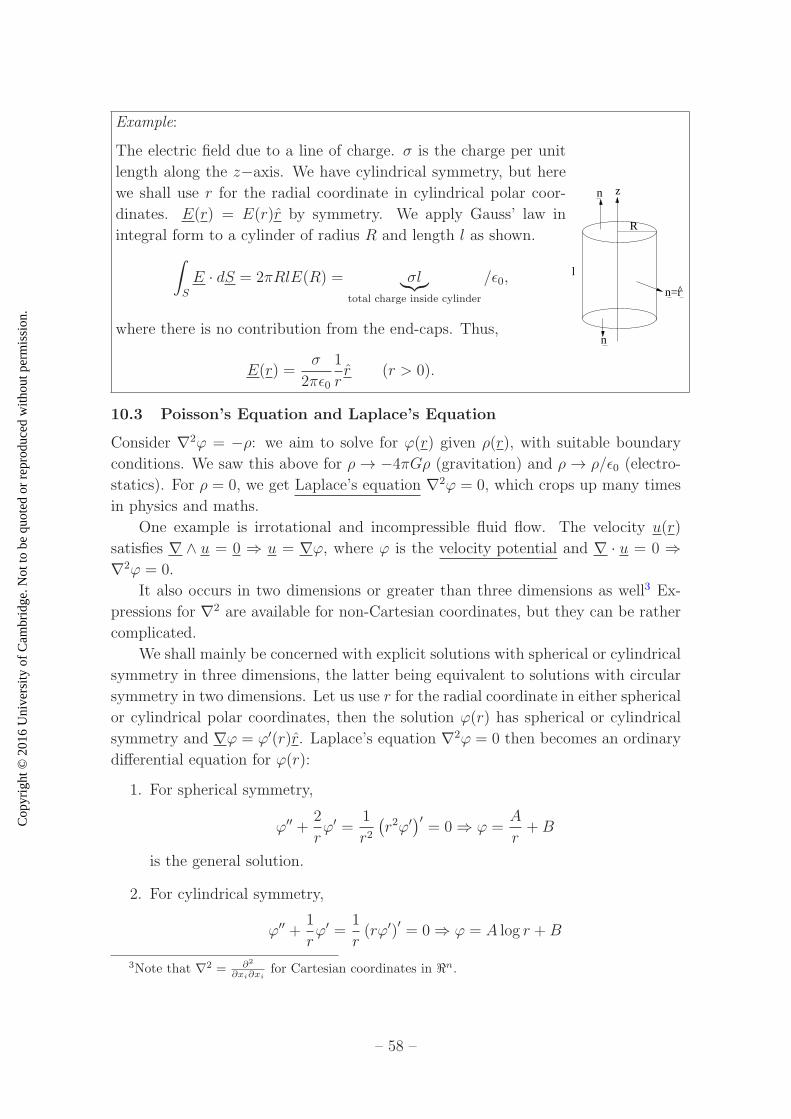
Cop
yrig
ht ©
201
6 U
nive
rsity
of C
ambr
idge
. Not
to b
e qu
oted
or
repr
oduc
ed w
ithou
t per
mis
sion
.
Example:
The electric field due to a line of charge. σ is the charge per unit
length along the z−axis. We have cylindrical symmetry, but here
we shall use r for the radial coordinate in cylindrical polar coor-
dinates. E(r) = E(r)r by symmetry. We apply Gauss’ law in
integral form to a cylinder of radius R and length l as shown.
∫
S
E · dS = 2πRlE(R) = σl︸︷︷︸
total charge inside cylinder
/ǫ0,
where there is no contribution from the end-caps. Thus,
E(r) =σ
2πǫ0
1
rr (r > 0).
l
R
n=r
n
n
z
^
10.3 Poisson’s Equation and Laplace’s Equation
Consider ∇2ϕ = −ρ: we aim to solve for ϕ(r) given ρ(r), with suitable boundary
conditions. We saw this above for ρ→ −4πGρ (gravitation) and ρ→ ρ/ǫ0 (electro-
statics). For ρ = 0, we get Laplace’s equation ∇2ϕ = 0, which crops up many times
in physics and maths.
One example is irrotational and incompressible fluid flow. The velocity u(r)
satisfies ∇ ∧ u = 0 ⇒ u = ∇ϕ, where ϕ is the velocity potential and ∇ · u = 0 ⇒∇2ϕ = 0.
It also occurs in two dimensions or greater than three dimensions as well3 Ex-
pressions for ∇2 are available for non-Cartesian coordinates, but they can be rather
complicated.
We shall mainly be concerned with explicit solutions with spherical or cylindrical
symmetry in three dimensions, the latter being equivalent to solutions with circular
symmetry in two dimensions. Let us use r for the radial coordinate in either spherical
or cylindrical polar coordinates, then the solution ϕ(r) has spherical or cylindrical
symmetry and ∇ϕ = ϕ′(r)r. Laplace’s equation ∇2ϕ = 0 then becomes an ordinary
differential equation for ϕ(r):
1. For spherical symmetry,
ϕ′′ +2
rϕ′ =
1
r2(r2ϕ′)′ = 0⇒ ϕ =
A
r+B
is the general solution.
2. For cylindrical symmetry,
ϕ′′ +1
rϕ′ =
1
r(rϕ′)
′= 0⇒ ϕ = A log r +B
3Note that ∇2 = ∂2
∂xi∂xi
for Cartesian coordinates in ℜn.
– 58 –

Cop
yrig
ht ©
201
6 U
nive
rsity
of C
ambr
idge
. Not
to b
e qu
oted
or
repr
oduc
ed w
ithou
t per
mis
sion
.
is the general solution.
Solutions to Poisson’s equation can be obtained in a similar way (i.e. by integrating
the differential equation directly) or by adding particular integrals to the discussions
above.
Example: Consider spherically symmetric solutions of ∇2ϕ = −ρ0, a constant. Note
that from section 6.2, ∇2(rα) = α(α + 1)rα−2 so α = 2 gives the particular integral
−16ρ0r
2. The general solution with spherical symmetry is then
ϕ(r) =A
r+ B
︸ ︷︷ ︸
general solution of Laplace’s equation
− 1
6ρ0r
2
︸ ︷︷ ︸
particular integral
.
For a unique solution to Poisson’s (or Laplace’s) equation, we must specify the
boundary conditions. If ϕ is defined in all of ℜ3, we often require ϕ→ 0 as |r| → ∞.
If ϕ is a solution on a bounded volume V , then there are two common kinds of
boundary condition on ∂V :
1. Specify ϕ: a Dirichlet condition
2. Specify4 ∂ϕ∂n
= n · ∇ϕ: a Neumann condition, where n is an outward normal on
∂V .
The choice of boundary condition depends on the physical content, for example
specifying ∂ϕ/∂n corresponds to specifying the normal component of g or E. We
can also specify different boundary conditions on different boundary components.
4Notice the new notation of a derivative with respect to a vector!
– 59 –
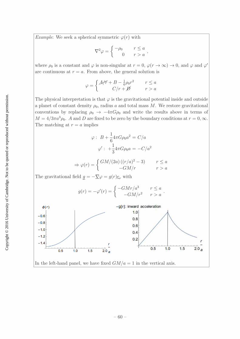
Cop
yrig
ht ©
201
6 U
nive
rsity
of C
ambr
idge
. Not
to b
e qu
oted
or
repr
oduc
ed w
ithou
t per
mis
sion
.
Example: We seek a spherical symmetric ϕ(r) with
∇2ϕ =
{−ρ0 r ≤ a
0 r > a,
where ρ0 is a constant and ϕ is non-singular at r = 0, ϕ(r →∞)→ 0, and ϕ and ϕ′
are continuous at r = a. From above, the general solution is
ϕ =
{
���A/r + B − 16ρ0r
2 r ≤ a
C/r +��D r > a
The physical interpretation is that ϕ is the gravitational potential inside and outside
a planet of constant density ρ0, radius a and total mass M . We restore gravitational
conventions by replacing ρ0 → −4πGρ0 and write the results above in terms of
M = 4/3πa3ρ0. A andD are fixed to be zero by the boundary conditions at r = 0,∞.
The matching at r = a implies
ϕ : B +1
64πGρ0a
2 = C/a
ϕ′ : +1
34πGρ0a = −C/a2
⇒ ϕ(r) =
{GM/(2a) ((r/a)2 − 3) r ≤ a
−GM/r r > a
The gravitational field g = −∇ϕ = g(r)er with
g(r) = −ϕ′(r) =
{−GMr/a3 r ≤ a
−GM/r2 r > a.
In the left-hand panel, we have fixed GM/a = 1 in the vertical axis.
– 60 –
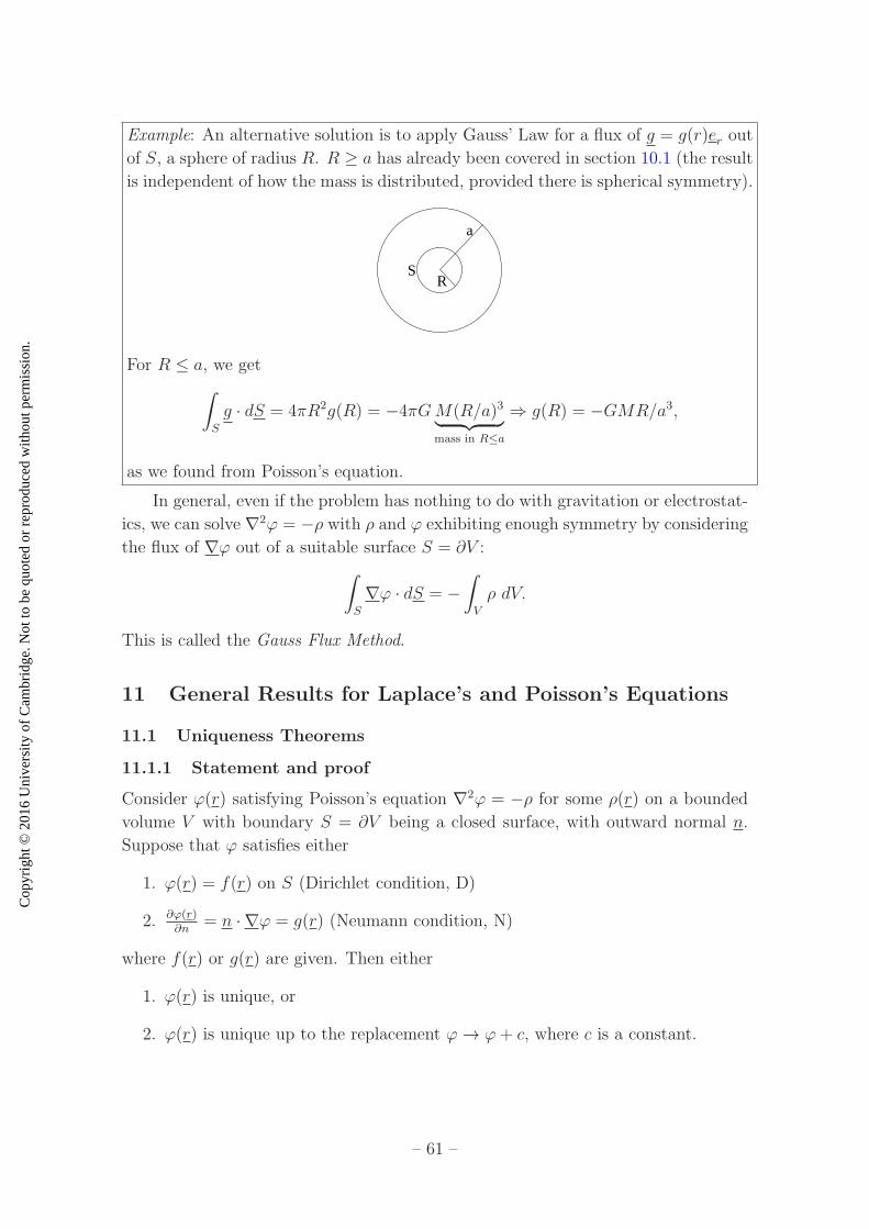
Cop
yrig
ht ©
201
6 U
nive
rsity
of C
ambr
idge
. Not
to b
e qu
oted
or
repr
oduc
ed w
ithou
t per
mis
sion
.
Example: An alternative solution is to apply Gauss’ Law for a flux of g = g(r)er out
of S, a sphere of radius R. R ≥ a has already been covered in section 10.1 (the result
is independent of how the mass is distributed, provided there is spherical symmetry).
a
RS
For R ≤ a, we get
∫
S
g · dS = 4πR2g(R) = −4πGM(R/a)3︸ ︷︷ ︸
mass in R≤a
⇒ g(R) = −GMR/a3,
as we found from Poisson’s equation.
In general, even if the problem has nothing to do with gravitation or electrostat-
ics, we can solve ∇2ϕ = −ρ with ρ and ϕ exhibiting enough symmetry by considering
the flux of ∇ϕ out of a suitable surface S = ∂V :
∫
S
∇ϕ · dS = −∫
V
ρ dV.
This is called the Gauss Flux Method.
11 General Results for Laplace’s and Poisson’s Equations
11.1 Uniqueness Theorems
11.1.1 Statement and proof
Consider ϕ(r) satisfying Poisson’s equation ∇2ϕ = −ρ for some ρ(r) on a bounded
volume V with boundary S = ∂V being a closed surface, with outward normal n.
Suppose that ϕ satisfies either
1. ϕ(r) = f(r) on S (Dirichlet condition, D)
2. ∂ϕ(r)∂n
= n · ∇ϕ = g(r) (Neumann condition, N)
where f(r) or g(r) are given. Then either
1. ϕ(r) is unique, or
2. ϕ(r) is unique up to the replacement ϕ→ ϕ+ c, where c is a constant.
– 61 –
Cop
yrig
ht ©
201
6 U
nive
rsity
of C
ambr
idge
. Not
to b
e qu
oted
or
repr
oduc
ed w
ithou
t per
mis
sion
.
Proof: Let ϕ1(r) and ϕ2(r) satisfy Poisson’s equation, each obeying the boundary
conditions (1) or (2). Then ψ(r) = ϕ2(r)−ϕ1(r) satisfies ∇2ψ = 0 on V by linearity
and (D) ψ = 0 on S or (N) ∂ψ/∂n = n · ∇ψ = 0 on S. By the divergence theorem,∫
V∇ · (ψ∇ψ) dV =
∫
Sψ∇ψ · dS. But
∇ · (ψ∇ψ) = ∇ψ · ∇ψ + ψ∇2ψ︸ ︷︷ ︸
0 on V
= |∇ψ|2.
So ∫
V
|∇ψ|2 dV =
∫
S
ψ∂ψ
∂ndS = 0
by either (N) or (D). Since |∇ψ|2 ≥ 0, the integral can only vanish if |∇ψ| = 0 ⇒∇ψ = 0⇒ ψ = c, a constant, on V . So:
(D) ψ = 0 on S ⇒ c = 0 and ϕ1 = ϕ2 on V , or
(N) ϕ2(r) = ϕ1(r) + c as claimed.
11.1.2 Comments
• The result says nothing about existence. Indeed, for ∇2ϕ = −ρ on V with∂ϕ∂n
= g on ∂V (Neumann) there can only be a solution if
∫
V
∇2ϕ dV =
∫
∂V
∂ϕ
∂ndS ⇔
∫
V
ρ dV +
∫
∂V
g dS = 0, (11.1)
but ρ and g are fixed to begin with, so Eq. 11.1 may not necessarily be true.
• The uniqueness result has practical importance: if we can find a solution by any
means, then we know it is the only solution. For example: find a solution with
symmetry ϕ(r), or more generally, linear combinations of separable solutions5
ϕ = X(x)Y (y) or R(r)Y (θ).
• The theorem can be stated and proved similarly for regions in ℜ2,3,...: it just
uses definitions of grad and div, and the divergence theorem.
• The results extend to unbounded domains, for example a sphere of radius R,
with |ψ(r)| = O(1/R) and |∂ψ∂n(r| = O(1/R2) for |r| = R ⇒ |
∫
Sψ ∂ψ∂n
dS| =O(1/R)→ 0 as R→∞. This last result follows because
∫
S
ψ∂ψ
∂ndS ≤ max|r|=R|ψ
∂ψ
∂n| × 4πR2 ≤ constant× (
1
R
1
R2)4πR2 = O( 1
R).
These conditions on ψ are ensured by taking for example |ψ(r)| = O(1/R)and ∇ψ(r)| = O(1/R2). Therefore, the proof extends to V = ℜ3 with these
boundary conditions as R = |r| → ∞ (S is the “sphere at infinity”).
5See Part IB Methods.
– 62 –

Cop
yrig
ht ©
201
6 U
nive
rsity
of C
ambr
idge
. Not
to b
e qu
oted
or
repr
oduc
ed w
ithou
t per
mis
sion
.
• Similar results apply to related equations and various kinds of boundary con-
ditions, perhaps with D or N being different parts of the boundary:
or
• The proof uses a special case of the result∫
S
(u∇v) · dS =
∫
V
∇u · ∇v dV +
∫
V
u∇2v dV,
sometimes called Green’s First Identity. Antisymmetrising in u and v gives∫
S
(u∇v − v∇u) dS =
∫
V
(u∇2v − v∇2u
)dV,
sometimes called Green’s Second Identity.
11.2 Laplace’s Equation and Harmonic Functions
Solutions of Laplace’s equation ∇2ϕ = 0 are also called harmonic functions. They
arise in many areas of physics and mathematics and have some very special proper-
ties.
11.2.1 The Mean Value Property
Suppose ϕ(r) is harmonic in a region V containing a solid sphere VR : |r − a| ≤ R
with boundary SR : |r − a| = R. Then ϕ(a) = ϕ(R) where
ϕ(R) =1
4πR2
∫
SR
ϕ(r) dS,
the average of ϕ over SR.
Proof: Note that ϕ(R) → ϕ(a) as R → 0. Take spherical polar coordinates
(u, θ, χ) centred on r = a. Then, the scalar area element on SR is (u = R) dS =
R2 sin θ dθ dχ⇒ dS/R2 is independent of R. Hence
d
dRϕ(R) =
1
4πR2
∫
SR
∂ϕ
∂u
∣∣∣∣u=R
dS.
But ∂ϕ∂u
= eu · ∇ϕ = n · ∇ϕ = ∂ϕ∂n
on SR.
⇒ dϕ(R)
dR=
1
4πR2
∫
SR
∇ϕ · dS =1
4πR2
∫
VR
∇2ϕ dV = 0.
So ϕ(R) is independent of R, and the result follows.
– 63 –
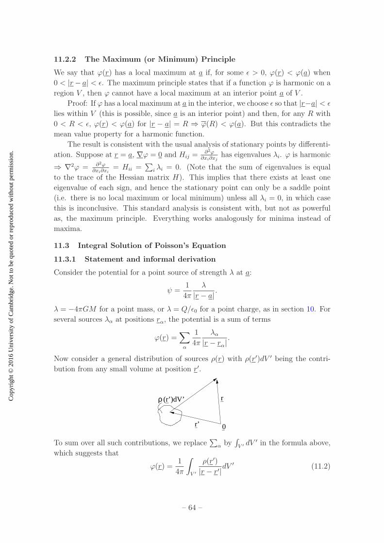
Cop
yrig
ht ©
201
6 U
nive
rsity
of C
ambr
idge
. Not
to b
e qu
oted
or
repr
oduc
ed w
ithou
t per
mis
sion
.
11.2.2 The Maximum (or Minimum) Principle
We say that ϕ(r) has a local maximum at a if, for some ǫ > 0, ϕ(r) < ϕ(a) when
0 < |r− a| < ǫ. The maximum principle states that if a function ϕ is harmonic on a
region V , then ϕ cannot have a local maximum at an interior point a of V .
Proof: If ϕ has a local maximum at a in the interior, we choose ǫ so that |r−a| < ǫ
lies within V (this is possible, since a is an interior point) and then, for any R with
0 < R < ǫ, ϕ(r) < ϕ(a) for |r − a| = R ⇒ ϕ(R) < ϕ(a). But this contradicts the
mean value property for a harmonic function.
The result is consistent with the usual analysis of stationary points by differenti-
ation. Suppose at r = a, ∇ϕ = 0 and Hij =∂2ϕ
∂xi∂xjhas eigenvalues λi. ϕ is harmonic
⇒ ∇2ϕ = ∂2ϕ∂xi∂xi
= Hii =∑
i λi = 0. (Note that the sum of eigenvalues is equal
to the trace of the Hessian matrix H). This implies that there exists at least one
eigenvalue of each sign, and hence the stationary point can only be a saddle point
(i.e. there is no local maximum or local minimum) unless all λi = 0, in which case
this is inconclusive. This standard analysis is consistent with, but not as powerful
as, the maximum principle. Everything works analogously for minima instead of
maxima.
11.3 Integral Solution of Poisson’s Equation
11.3.1 Statement and informal derivation
Consider the potential for a point source of strength λ at a:
ψ =1
4π
λ
|r − a| .
λ = −4πGM for a point mass, or λ = Q/ǫ0 for a point charge, as in section 10. For
several sources λα at positions rα, the potential is a sum of terms
ϕ(r) =∑
α
1
4π
λα|r − rα|
.
Now consider a general distribution of sources ρ(r) with ρ(r′)dV ′ being the contri-
bution from any small volume at position r′.
0r’
r(r’)dV’ρ
To sum over all such contributions, we replace∑
α by∫
V ′dV ′ in the formula above,
which suggests that
ϕ(r) =1
4π
∫
V ′
ρ(r′)
|r − r′|dV′ (11.2)
– 64 –
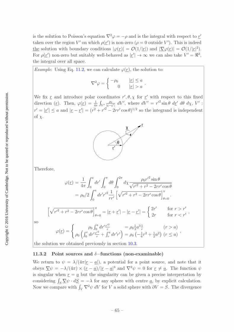
Cop
yrig
ht ©
201
6 U
nive
rsity
of C
ambr
idge
. Not
to b
e qu
oted
or
repr
oduc
ed w
ithou
t per
mis
sion
.
is the solution to Poisson’s equation ∇2ϕ = −ρ and is the integral with respect to r′
taken over the region V ′ on which ρ(r′) is non-zero (ρ = 0 outside V ′). This is indeed
the solution with boundary conditions |ϕ(r)| = O(1/|r|) and |∇ϕ(r)| = O(1/|r|2).For ρ(r′) non-zero but suitably well-behaved as |r′| → ∞ we can also take V ′ = ℜ3,
the integral over all space.
Example: Using Eq. 11.2, we can calculate ϕ(r), the solution to:
∇2ϕ =
{−ρ0 |r| ≤ a
0 |r| > a.
We fix r and introduce polar coordinates r′, θ, χ for r′ with respect to this fixed
direction (r). Then, ϕ(r) = 14π
∫
V ′
ρ0|r−r′| dV
′, where dV ′ = r′2 sin θ dr′ dθ dχ, V ′ :
r′ = |r′| ≤ a and |r − r′| = (r2 + r′2 − 2rr′ cos θ)1/2 so the integrand is independent
of χ.
r
r’
χ
θ
Therefore,
ϕ(r) =1
4π
∫ a
0
dr′∫ π
0
dθ
∫ 2π
0
dχρ0r
′2 sin θ√r′2 + r2 − 2rr′ cos θ
= ρ0/2
∫ a
0
dr′r′2 1
rr′
[√
r′2 + r2 − 2rr′ cos θ]π
θ=0.
[√
r′2 + r2 − 2rr′ cos θ]π
θ=0= |r + r′| − |r − r′| =
{2r′ for r > r′
2r for r < r′,
so
ϕ(r) =
{
ρ0∫ a
0dr′ r
′2
r= ρ0
13a3 1
r(r > a)
ρ0
(∫ r
0dr′ r
′2
r+∫ a
rdr′r′
)
= ρ0(−1
6r2 + 1
2a2)(r ≤ a)
,
the solution we obtained previously in section 10.3.
11.3.2 Point sources and δ−functions (non-examinable)
We return to ψ = λ/(4π|r − a|), a potential for a point source, and note that it
obeys ∇ψ = −λ/(4π) × (r − a)/|r − a|3 and ∇2ψ = 0 for r 6= a. The function ψ
is singular when r = a but the singularity can be given a precise interpretation by
considering∫
S∇ψ · dS = −λ for any sphere with centre a, by explicit calculation.
Now we compare with∫
V∇2ψ dV for V a solid sphere with ∂V = S. The divergence
– 65 –

Cop
yrig
ht ©
201
6 U
nive
rsity
of C
ambr
idge
. Not
to b
e qu
oted
or
repr
oduc
ed w
ithou
t per
mis
sion
.
theorem holds if we take∇2ψ = −λδ(r−a) where6 the three-dimension delta function
is a generalised function (or distribution) satisfying∫
Vf(r)δ(r−a) dV = f(a) for any
volume V containing a. Using this, we can verify the integral solutions of Poisson’s
equations immediately:
∇2ψ(r) =1
4π
∫
V ′
ρ(r′)∇2 1
|r − r′|dV′ = −
∫
V ′
ρ(r′)δ(r − r′)dV ′ = −ρ(r),
as required.
12 Maxwell’s Equations
12.1 Laws of Electromagnetism
Static electric charges interact in a way that is mathematically almost identical to
gravitational interactions. More generally, moving electric charges interact in a way
that can be described by electric and magnetic fields E(r, t) and B(r, t).
If ρ(r, t) is the charge density and j(r, t) the current density, then the resulting
electric and magnetic fields are determined by Maxwell’s equations:
∇ · E = ρǫ0
∇∧ E +∂B
∂t= 0
∇ ·B = 0 ∇∧ B − µ0ǫ0∂E
∂t= µ0j,
where ǫ0 is the permittivity of free space and µ0 is the permeability of free space
(they are both physical constants). Then, the Lorentz Force on a point charge q due
to these fields is
F = q(E + r ∧B).
In principle, this gives a complete description of all classical electromagnetic phe-
nomena.
Conservation of electric charge comes from Maxwell’s equations:
∂ρ
∂t+∇ · j = 0.
Gauss’ Law for E is unmodified, and now we have a similar law for B too (in
electrostatics), but with zero ‘magnetic charge’. In integral form:∫
S
E · dS = Q/ǫ0,
∫
S
B · dS = 0.
The remaining Maxwell’s equations also have integral forms, for example∫
CE ·dr =
− ddt
∫
SB · dS for any surface S with a boundary of a closed curve C, from Stokes’
theorem.
6The expression for ∇2ψ above makes sense intuitively for a point source concentrated at a.
– 66 –
Cop
yrig
ht ©
201
6 U
nive
rsity
of C
ambr
idge
. Not
to b
e qu
oted
or
repr
oduc
ed w
ithou
t per
mis
sion
.
12.2 Static Charges and Steady Currents
If ρ, j, E and B are all independent of time, then E and B are no longer linked, since
Maxwell’s equations then imply:
Electrostatics Magnetostatics
∇ · E = ρ/ǫ0 ∇ · B = 0
∇∧ E = 0 ∇∧ B = µ0j
⇒ E = −∇ϕ and ∇2ϕ = −ρ/ǫ0, the scalar ⇒ B = ∇∧ A, but the vector potential is
Poisson equation described in section 11.3. ambiguous: A→ A+∇χ produces the same
B field. The scalar field χ can be chosen to
make ∇ · A = 0⇒ ∇2A = −µ0j, the vector
Poisson equation: it has a similar general
solution to the scalar case.
ǫ0 sets the scale of electrostatic effects, µ0 sets the scale of magnetic effects, for
for example the Coulomb force. example the force between current-carrying
wires.
12.3 Electromagnetic Waves
Consider Maxwell’s equations with ρ = 0 and j = 0 (i.e. empty space):
∇2E = ∇(∇·E)−∇∧ (∇∧E) = ∇∧ ∂B∂t
=∂
∂t(∇∧B) =
∂
∂t(µ0ǫ0
∂E
∂t) = µ0ǫ0
∂2E
∂t2,
or(
∇2 − 1
c2∂2
∂t2
)
E = 0, and similarly we can obtain
(
∇2 − 1
c2∂2
∂t2
)
B = 0,
where c2 = 1/(ǫ0µ0). These are wave equations in three dimensions describing prop-
agation with speed c. We compare with the one dimensional wave equation for a
scalar (∂2
∂x2− 1
c2∂2
∂t2
)
f = 0, f = f±(x∓ ct)
where f+ describes a right moving wave and f− a left moving wave.
So, Maxwell’s equations predict electromagnetic waves which move with speed
c = 1/√ǫ0µ0 ≈ 2.998× 10⁸ ms−1, i.e. the experimentally measured values of µ0 and
ǫ0 combine to give the experimental value of the speed of light.
Maxwell famously said “We can scarcely avoid the inference that light consists of
the transverse modulation of the same medium which is the cause of electric and mag-
netic phenomena”. This was the unification of the theories of electricity, magnetism
and light.
– 67 –

Cop
yrig
ht ©
201
6 U
nive
rsity
of C
ambr
idge
. Not
to b
e qu
oted
or
repr
oduc
ed w
ithou
t per
mis
sion
.
13 Tensors and Tensor Fields
13.1 Definitions and Examples
13.1.1 Tensor transformation rule
Consider orthonormal right-handed bases {ei} and {e′i} in ℜ3 with corresponding
Cartesian coordinates {xi} and {x′i}: x = xiei = x′iei′. Any such bases are related
by a rotation: e′i = Ripep, x′i = Ripxp where
1. RipRjp = RqiRqj = δij or RRT = RTR = I, in other words R is orthogonal.
2. detR = 1, or R is special orthogonal.
The components of a vector v transform in a similar way under this change of basis
and coordinates: v = viei = v′ie′i ⇒ v′i = Ripvp.
Tensors are geometric objects which obey a generalised form of this transfor-
mation rule. By definition, a tensor T of rank n has components Tij...k (n indices)
with respect to each basis {ei} or coordinate system {xi} and under a change of
basis/coordinates
T ′ij...k = RipRjq . . . RkrTpq...r.
This is the tensor transformation rule.
Examples:
T of rank 0, i.e. no indices T = T ′, a scalar
T of rank 1, T ′i = RipTp, a vector
T of rank 2, T ′ij = RipRjqTpq form a matrix.
13.1.2 Basic examples
1. If u, v, . . . , w are n vectors, then Tij...k = uivj . . . wk defines a tensor of rank n.
To show this, we check the transformation rule. For example n = 2, Tij = uivj.
T ′ij = u′iv
′j = (Ripup)(Rjqvq) = RipRjq(upvq) = RipRjqTpq,
i.e the correct rule. Any linear combination of such expressions are also tensors,
for example Tij = uivj + aibj for any u, v, a, b.
2. δij and ǫijk are tensors of rank 2 and 3 respectively, with the special property
that their components are unchanged with respect to any basis/coordinate
system: δ′ij = RipRjqδpq = RipRjp = δij which is the tensor transformation
rule with δ′ij = δij and RipRjqRkrǫpqr = (detR)ǫijk = ǫijk which7 is the tensor
transformation rule with ǫ′ijk = ǫijk.
7Note that here, we used a general result from Vectors and Matrices IA, namely
MipMjqMkrǫpqr = (detM)ǫijk.
– 68 –

Cop
yrig
ht ©
201
6 U
nive
rsity
of C
ambr
idge
. Not
to b
e qu
oted
or
repr
oduc
ed w
ithou
t per
mis
sion
.
13.1.3 Rank 2 tensors and matrices
A linear map between vectors u and v has the general form vi =Mijuj or v′i =M ′
iju′j
with respect to different choices of basis/coordinate system. Using the transformation
rule for vectors: v′i = Ripvp = Rip(Mpquq) = M ′iju
′j = M ′
ij(Rjquq). These expressions
are compatible for any u iff RipMpq = M ′ijRjq or M ′
ik = RipRkqMpq; this is the
tensor transformation rule for rank 2. In matrix notation M ′ = RMRT , which is the
standard transformation for the matrix of a linear map under an orthogonal change
of basis (RT = R−1).
Example: In many substances, an applied electric field E induces an electric current
density j according to the linear relation (Ohm’s Law) ji = σikEk, where σik is
the conductivity tensor (it is automatically a tensor, by the argument given above).
Substances may conduct differently in different directions (for example if they have
a layered structure) and then j is not parallel to E in general. For an isotropic
substance, σik = σδik ⇒ j = σE.
13.2 Tensor Algebra
13.2.1 Addition and scalar multiplication
Tensors T and S of the same rank can be added; T + S is also a tensor of rank n
defined by (T + S)ij...k = Tij...k + Sij...k in any coordinate system. To show that this
is a tensor, we check the transformation rule, for example for n = 2:
(T +S)′ij = T ′ij+S
′ij = RipRjqTpq+RipRjqSpq = RipRjq(Tpq+Spq) = RipRjq(T +S)pq.
A tensor T of any rank can be multiplied by a scalar α; αT is a tensor of the
same rank, defined by αTij...k = αTij...k in any coordinate system (it’s easy to check
the transformation rule).
13.2.2 Tensor products
If T and S are tensors of rank n and m then the tensor product T ⊗ S is a tensor of
rank n+m defined by
(T ⊗ S)ij . . . k︸ ︷︷ ︸n indices
pq . . . r︸ ︷︷ ︸m indices
= Tij...kSpq...r.
This is a tensor (check the transformation rule yourself). The tensor product can be
defined similarly for any number of tensors, for example for n vectors u, v, . . . w we
define T = u⊗ v · · · ⊗ w by Tij...k = uivj · · ·wk as in section 13.1.
13.2.3 Contractions
Given a rank n tensor T with components Tijp...q, we define a new tensor S of rank
n − 2 by Sp...q = δijTijp...q = Tiip...q. This is called contracting on the indices i and
– 69 –

Cop
yrig
ht ©
201
6 U
nive
rsity
of C
ambr
idge
. Not
to b
e qu
oted
or
repr
oduc
ed w
ithou
t per
mis
sion
.
j. Contracting on a different pair of indices results in a different tensor, in general.
To check that contraction produces a tensor, we take the example of Tij of rank 2.
Contracting Tii of rank 0 (i.e. a scalar), T ′ii = RipRiqTpq = δpqTpq = Tpp. Higher rank
tensors involve additional indices that are unaffected by the contraction. Note that
with Tij regarded as a 3 by 3 matrix, Tii is the trace. T ′ii = Tr(T ′) = Tr(RTRT ) =
Tr(T ) = Tpp, in matrix language.
13.2.4 Symmetric and antisymmetric tensors
A tensor T of rank n obeying Tijp...q = ±Tjip...q is said to be symmetric (+) or anti-
symmetric (-) in the indices i and j. (There exists a similar definition for any other
index pair). This holds in all coordinate systems if it holds in any one, since
T ′klr...s = RkiRljRrp . . . RsqTijp...q = ±RkiRljRrp . . . RsqTjip...q = ±T ′
lkr...s.
A tensor is called totally symmetric/anti-symmetric if it is symmetric/anti-symmetric
in every pair of indices. For example δij = δji is totally symmetric and ǫijk is totally
anti-symmetric. There are totally symmetric tensors of arbitrary rank n, but in ℜ3:
1. Any totally antisymmetric tensor of rank 3 has the form Tijk = λǫijk for some
scalar λ.
2. There are no totally antisymmetric tensors of rank n > 3 except (trivially) the
tensors with all components zero.
13.3 Tensors, Multi-linear Maps and the Quotient Rule
13.3.1 Tensors as multi-linear maps
A tensor T of rank n is equivalent to a multi-linear map from n vectors a, b, . . . c to
ℜ defined by
T (a, b, . . . , c) =
(1)︷ ︸︸ ︷
Tij...kaibj . . . ck =
(2)︷ ︸︸ ︷
T ′pq...ra
′pb
′q . . . c
′r .
‘Multi-linear’ means that T is linear in each of the vectors a, b, . . . , c individually.
Note that
1. If the first expression (1) is specified for all vectors a, b, . . . , c then the com-
ponents of the tensor are uniquely determined (by taking a, b, . . . , c to be all
possible choices of basis vectors).
2. Using the standard relationship for vector components v′p = Rpivi or vi = Rpiv′p,
(1) and (2) agree iff Tij...kRpia′pRqjb
′q . . . Rrkc
′r = T ′
pq...ra′pb
′q . . . c
′r, which holds for
any a′pb′q . . . c
′r iff T
′pq...r = RpiRqj . . . RrkTij...k, ie the transformation rule. Thus,
there is a one-to-one correspondence between tensors of rank n and multi-
linear maps. This gives a way of thinking about tensors’ independent of any
coordinate system or choice of basis, and the tensor transformation rule emerges
naturally.
– 70 –
Cop
yrig
ht ©
201
6 U
nive
rsity
of C
ambr
idge
. Not
to b
e qu
oted
or
repr
oduc
ed w
ithou
t per
mis
sion
.
13.3.2 The quotient rule
If Ti . . . j︸ ︷︷ ︸
n
p . . . q︸ ︷︷ ︸
m
is a tensor of rank n+m and up...q is any tensor of rank m, then
vi...j = Ti...jp...qup...q
is a tensor of rank n (it is a tensor product of T and u, followed by contractions).
Conversely, suppose that Ti...jp...q is an array defined for each coordinate system,
and that for any tensor up...q, vi...j as defined above is also a tensor, then Ti...jp...q is
also a tensor.
This is the quotient rule. We have seen and proved the special case n = m = 1
in section 13.1.3. The general case can be proved in a similar way, checking the
transformation rule directly, but the proliferation of indices makes the argument
look more complicated than it really is.
To streamline things, we shall use the ideas in section 13.3.1. It is sufficient to
take the special form up...q = cp . . . dq for any vectors c, . . . , d; by assumption vi...j =
Ti...jp...qcp . . . dq is a tensor, but then vi...jai . . . bj = Ti...jp...qai . . . bjcp . . . dq is a scalar
for any vectors a, . . . , b, c, . . . d. This is enough to ensure the tensor transformation
rule for the components Ti...jp...q, as observed in section 13.3.1 above.
13.4 Tensor Calculus
13.4.1 Tensor fields and derivatives
Just as with scalars or vectors, a tensor field is a tensor at each point Tij...k(x), which
we also write as8 Tij...k(xl). We assume that fields are smooth so that they can be
differentiated any number of times
∂
∂xp. . .
∂
∂xq︸ ︷︷ ︸
m
Tij . . . k︸ ︷︷ ︸
n
,
except for where things obviously fail, for example where T is not defined. This is a
new tensor of rank n+m.
To verify the transformation rule, consider the derivatives: x′i = Ripxp ⇒ ∂x′i∂xp
=
Rip, and xq = (R−1)qix′i = Riqx
′i ⇒ ∂xq
∂x′i= Riq. Note that Rip and Riq are constant
matrices. Now, by the chain rule
∂
∂x′i=∂xq∂x′i
∂
∂xq= Riq
∂
∂xq.
This is expected for components of a vector, and as emphasised in section 9.2,
∇ = ei∂/∂xi = e′i∂/∂x′i is a vector operator. Using this, it is easy to check the
8Meaning that it can depend upon all of the coordinates
– 71 –
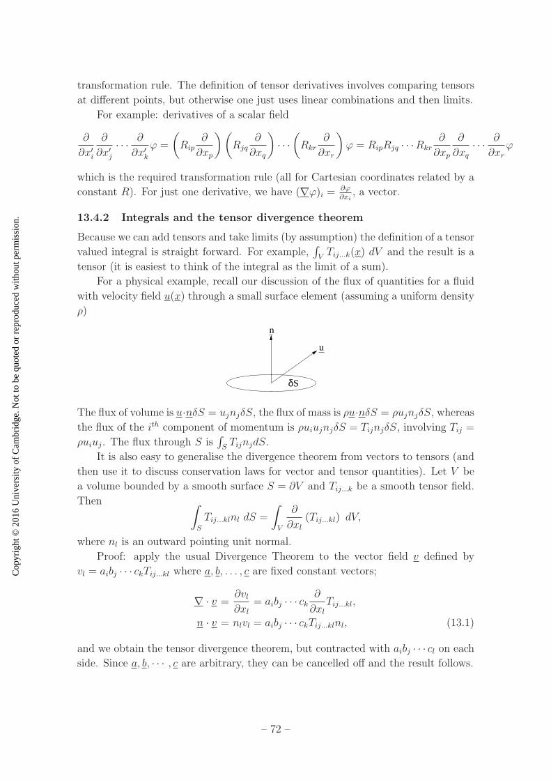
Cop
yrig
ht ©
201
6 U
nive
rsity
of C
ambr
idge
. Not
to b
e qu
oted
or
repr
oduc
ed w
ithou
t per
mis
sion
.
transformation rule. The definition of tensor derivatives involves comparing tensors
at different points, but otherwise one just uses linear combinations and then limits.
For example: derivatives of a scalar field
∂
∂x′i
∂
∂x′j· · · ∂
∂x′kϕ =
(
Rip∂
∂xp
)(
Rjq∂
∂xq
)
· · ·(
Rkr∂
∂xr
)
ϕ = RipRjq · · ·Rkr∂
∂xp
∂
∂xq· · · ∂
∂xrϕ
which is the required transformation rule (all for Cartesian coordinates related by a
constant R). For just one derivative, we have (∇ϕ)i = ∂ϕ∂xi
, a vector.
13.4.2 Integrals and the tensor divergence theorem
Because we can add tensors and take limits (by assumption) the definition of a tensor
valued integral is straight forward. For example,∫
VTij...k(x) dV and the result is a
tensor (it is easiest to think of the integral as the limit of a sum).
For a physical example, recall our discussion of the flux of quantities for a fluid
with velocity field u(x) through a small surface element (assuming a uniform density
ρ)
n
u
Sδ
The flux of volume is u·nδS = ujnjδS, the flux of mass is ρu·nδS = ρujnjδS, whereas
the flux of the ith component of momentum is ρuiujnjδS = TijnjδS, involving Tij =
ρuiuj. The flux through S is∫
STijnjdS.
It is also easy to generalise the divergence theorem from vectors to tensors (and
then use it to discuss conservation laws for vector and tensor quantities). Let V be
a volume bounded by a smooth surface S = ∂V and Tij...k be a smooth tensor field.
Then ∫
S
Tij...klnl dS =
∫
V
∂
∂xl(Tij...kl) dV,
where nl is an outward pointing unit normal.
Proof: apply the usual Divergence Theorem to the vector field v defined by
vl = aibj · · · ckTij...kl where a, b, . . . , c are fixed constant vectors;
∇ · v =∂vl∂xl
= aibj · · · ck∂
∂xlTij...kl,
n · v = nlvl = aibj · · · ckTij...klnl, (13.1)
and we obtain the tensor divergence theorem, but contracted with aibj · · · cl on each
side. Since a, b, · · · , c are arbitrary, they can be cancelled off and the result follows.
– 72 –

Cop
yrig
ht ©
201
6 U
nive
rsity
of C
ambr
idge
. Not
to b
e qu
oted
or
repr
oduc
ed w
ithou
t per
mis
sion
.
14 Tensors of Rank 2
14.1 Decomposition of a Second Rank Tensor
Any second rank tensor can be written as a sum of its symmetric and anti-symmetric
parts: Tij = Sij + Aij has 9 independent components (IC), where Sij =12(Tij + Tji)
has 6 IC and Aij =12(Tij −Tji) has 3 IC. In fact, the symmetric part can be reduced
further: Sij = Pij +13δijQ where Pii = 0, or Pij is traceless, and Q = Sii is the trace
of Sij. Pij has 5 IC whereas Q has 1. The antisymmetric part can be re-expressed:
Aij = ǫijkBk ⇔ Bk =1
2ǫijkAij
from the double-ǫ identities, or
(Aij) =
0 B3 −B2
−B3 0 B1
B2 −B1 0
.
To summarise,
Tij = Pij︸︷︷︸
symmetric traceless
+ǫijk Bk︸︷︷︸
vector
+1
3δij Q︸︷︷︸
scalar
where Bk = 12ǫijkTij , and only the antisymmetric parts of T contribute. Qk = Tkk
where only symmetric parts of T contribute.
Example: A vector field Fi(r) derivative Tij =∂Fi
∂xj, a tensor field. The decomposition
given above has a symmetric traceless piece Pij =12(∂Fi
∂xj+
∂Fj
∂xi) − 1
3δij
∂Fk
∂xk, an anti-
symmetric piece Aij = ǫijkBk with Bk = 12ǫijk
∂Fi
∂xj= −1
2(∇ ∧ F )k and a trace Q =
∂Fk
∂xk= ∇ · F . Hence, a complete description of the derivative of a vector field F
involves a scalar ∇ · F , a vector ∇∧ F and a symmetric traceless tensor Pij .
14.2 The Inertia Tensor
Consider some masses mα with positions rα, all rotating with angular velocity ω
about 0, so the velocities are vα = ω ∧ rα. The total angular momentum about 0 is
L =∑
α
rα ∧mαvα =∑
α
mαrα ∧ (ω ∧ rα) =∑
α
mα
(|rα|2ω − rα(rα · ω)
).
In components, Li = Iijωj where
Iij =∑
α
mα
(|rα|2δij − (rα)i(rα)j
)
is the inertia tensor about 0. Note that in general L is not parallel to ω.
– 73 –
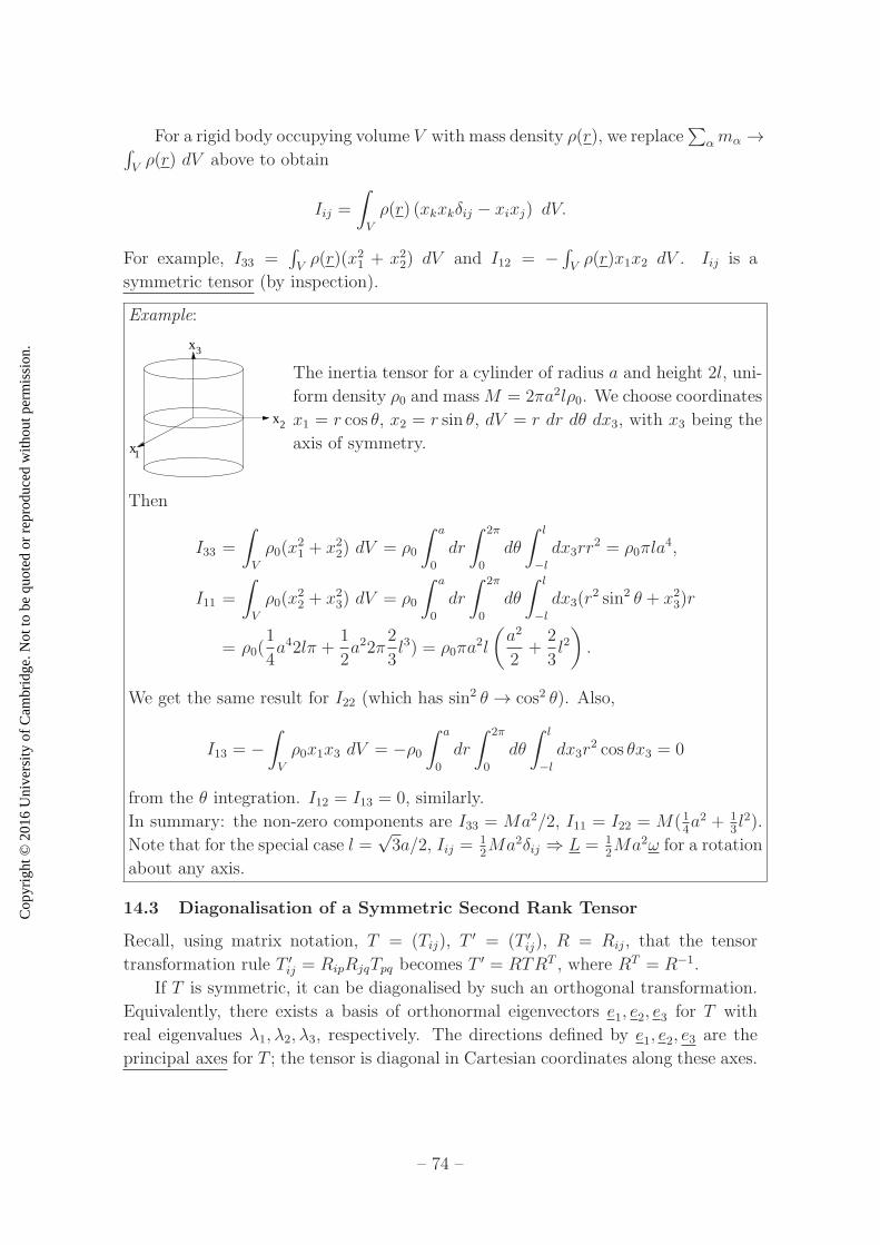
Cop
yrig
ht ©
201
6 U
nive
rsity
of C
ambr
idge
. Not
to b
e qu
oted
or
repr
oduc
ed w
ithou
t per
mis
sion
.
For a rigid body occupying volume V with mass density ρ(r), we replace∑
αmα →∫
Vρ(r) dV above to obtain
Iij =
∫
V
ρ(r) (xkxkδij − xixj) dV.
For example, I33 =∫
Vρ(r)(x21 + x22) dV and I12 = −
∫
Vρ(r)x1x2 dV . Iij is a
symmetric tensor (by inspection).
Example:
x
x
x1
2
3
The inertia tensor for a cylinder of radius a and height 2l, uni-
form density ρ0 and massM = 2πa2lρ0. We choose coordinates
x1 = r cos θ, x2 = r sin θ, dV = r dr dθ dx3, with x3 being the
axis of symmetry.
Then
I33 =
∫
V
ρ0(x21 + x22) dV = ρ0
∫ a
0
dr
∫ 2π
0
dθ
∫ l
−ldx3rr
2 = ρ0πla4,
I11 =
∫
V
ρ0(x22 + x23) dV = ρ0
∫ a
0
dr
∫ 2π
0
dθ
∫ l
−ldx3(r
2 sin2 θ + x23)r
= ρ0(1
4a42lπ +
1
2a22π
2
3l3) = ρ0πa
2l
(a2
2+
2
3l2)
.
We get the same result for I22 (which has sin2 θ → cos2 θ). Also,
I13 = −∫
V
ρ0x1x3 dV = −ρ0∫ a
0
dr
∫ 2π
0
dθ
∫ l
−ldx3r
2 cos θx3 = 0
from the θ integration. I12 = I13 = 0, similarly.
In summary: the non-zero components are I33 = Ma2/2, I11 = I22 = M(14a2 + 1
3l2).
Note that for the special case l =√3a/2, Iij =
12Ma2δij ⇒ L = 1
2Ma2ω for a rotation
about any axis.
14.3 Diagonalisation of a Symmetric Second Rank Tensor
Recall, using matrix notation, T = (Tij), T′ = (T ′
ij), R = Rij, that the tensor
transformation rule T ′ij = RipRjqTpq becomes T ′ = RTRT , where RT = R−1.
If T is symmetric, it can be diagonalised by such an orthogonal transformation.
Equivalently, there exists a basis of orthonormal eigenvectors e1, e2, e3 for T with
real eigenvalues λ1, λ2, λ3, respectively. The directions defined by e1, e2, e3 are the
principal axes for T ; the tensor is diagonal in Cartesian coordinates along these axes.
– 74 –
Cop
yrig
ht ©
201
6 U
nive
rsity
of C
ambr
idge
. Not
to b
e qu
oted
or
repr
oduc
ed w
ithou
t per
mis
sion
.
This applies to any symmetric tensor. For the special case of the inertia ten-
sor, the eigenvalues are called the principal moments of inertia. As exemplified in
section 14.2, we can often guess the correct principal axes for Iij based on the sym-
metries of the body: with the axes we chose, Iij was found to be diagonal, by direct
calculation.
15 Invariant and Isotropic Tensors
15.1 Definitions and Classification Results
A tensor T is invariant under a particular rotation R if
T ′ij...k = RipRjq · · ·RkrTpq···r = Tij···k,
i.e. each component is unchanged. A tensor T which is invariant under every rotation
is called isotropic (i.e. the same in all directions). As noted in section 13.1.2, δij and
ǫijk are isotropic tensors. This ensures that the component definitions of the scalar
and vector products
a · b = δijaibj, (a ∧ b)i = ǫijkajbk
are independent of the Cartesian coordinate system. Isotropic tensors in ℜ3 can be
classified:
1. There are no isotropic tensors of rank 1 (vector) except the zero vector.
2. The most general rank 2 isotropic tensor is Tij = αδij for some scalar α.
3. The most general rank 3 isotropic tensor is Tijk = βǫijk for some scalar β.
4. All isotropic tensors of higher rank are obtained by combining δij and ǫijk using
tensor products, contractions and linear combinations.
Example: The most general isotropic tensor of rank 4 is
Tijkl = αδijδkl + βδikδjl + γδilδjk
for some scalar constants α, β, γ. There are no other independent combinations (for
example, you might think of ǫijpǫklp, but this is equal to δikδjl − δilδjk).
15.2 Application to Invariant Integrals
Consider a tensor defined by
Tij...k =
∫
V
f(x)xixj · · · xkdV
– 75 –
Cop
yrig
ht ©
201
6 U
nive
rsity
of C
ambr
idge
. Not
to b
e qu
oted
or
repr
oduc
ed w
ithou
t per
mis
sion
.
with f(x) being a scalar function and V is some volume. Given a rotation Rij ,
consider an active transformation x = xiei mapped to x′ = x′iei with x′i = Rijxj (NB
there is no change of basis vectors here) and V is mapped to V ′. Suppose that under
this active transformation
1. f(x) = f(x′) and
2. V ′ = V .
Then Tij...k is invariant under Rij .
Proof:
RipRjq · · ·RkrTpq...r =
∫
V
f(x)x′ix′j · · · x′kdV
from the definition of T
=
∫
V
f(x′)x′ix′j · · · x′kdV
from (1)
=
∫
V ′
f(x′)x′ix′j · · · x′kdV ′
from (2)
= Tij...k
(xi or x′i are dummy variables in the integral).
NB with the change of variables x′i = Ripxp,∂x′i∂xp
= Rip (a constant) and
det(∂x′i∂xp
) = det(Rip) = 1, i.e. the Jacobian=1 or dV ′ = dV . The result is partic-
ularly useful if (1) and (2) hold for any rotation R, in which case Tij...k is isotropic.
Example: Tij =∫
Vxixj dV with V being a solid sphere with |r| ≤ a. The result
above applies with f = 1 for any rotation R, so Tij is isotropic ⇒ Tij = αδij , and
we need only determine the scalar α. But taking the trace, 3α = Tii =∫
Vxixi dV =
∫ a
0r24πr2 dr = 4
5πa5. Hence Tij =
415πa5δij .
There is a closely related result for the inertia tensor of a sphere of constant density
ρ0 or mass M :
Iij =
∫
V
ρ0 (xkxkδij − xixj) dV = ρ0(3− 1)4
15πa5δij =
2
5Ma2δij ,
which is isotropic.
15.3 A Sketch of a Proof of Classification Results for Rank n ≤ 3
The results follow straight forwardly by analysing conditions for invariance under
specific rotations through π or π/2 about coordinate axes, then confirming that the
most general form allowed is actually isotropic.
– 76 –
Cop
yrig
ht ©
201
6 U
nive
rsity
of C
ambr
idge
. Not
to b
e qu
oted
or
repr
oduc
ed w
ithou
t per
mis
sion
.
1. Suppose that Ti is rank 1 isotropic. Consider
(Rij) =
−1 0 0
0 −1 0
0 0 1
,
a rotation through π about the x3 axis. Then T1 = R1pTp = R11T1 = −T1 and
T2 = R2pTp = R22T2 = −T2. Then T1 = T2 = 0. Then, requiring isotropy of a
rotation through π about the x1 axis too yields T3 = 0, and therefore Ti = 0.
2. Suppose that Tij is rank 2 isotropic. Consider
(Rij) =
0 1 0
−1 0 0
0 0 1
,
a rotation through π/2 clockwise about the x3 axis: T13 = R1pR3qTpq =
R12R33T23 = (+1)(+1)T23. T23 = R2pR3qTpq = R21R33T13 = (−1)(+1)T13.
Hence T13 = T23 = 0 and similarly T31 = T32 = 0. T11 = R1pR1qTpq =
R12R12T22 = (+1)(+1)T22. By applying π/2 rotations about the x1 and x2axes in a similar way, we deduce T11 = T22 = T33 = α, say and Tij∀i 6= j.
Hence Tij = αδij .
3. Suppose that Tijk is rank 3 isotropic. Using the rotation by π as in (1)
above, T133 = R1pR3qR3rTpqr = (−1)(+1)(+1)T133 and T111 = R1pR1qR1rTpqr =
(−1)(−1)(−1)T111, with similar results for π rotations about other axes and
with other index positions we write Tijk = 0 unless i, j, k are all distinct. Now
consider a rotation through π/2 as in (2) above: T123 = R1pR2qR3rTpqr =
R12R21R33T213 = (+1)(−1)(+1)T213 = −T213. Along with similar results for
other index positions and other axes of rotation, Tijk is totally antisymmetric,
hence Tijk = βǫijk.
Acknowledgements
We thank Prof. R. Josza for proof reading.
– 77 –