COMPUTING COMPLEX SINGULARITIES OF DIFFERENTIALEQUATIONS WITH CHEBFUN

AUTHOR: MARCUS WEBB∗ AND ADVISOR: LLOYD N. TREFETHEN†

Abstract. Given a solution to an ordinary differential equation (ODE) on a time interval, thesolution for complex-valued time may be of interest, in particular whether the solution is singular atsome complex time value. How can the solution be approximated in the complex plane using only thedata on the interval? A polynomial approximation of the solution always fails to capture singularities;to extrapolate solutions with singularities, approximation with rational functions is more appropriate.In this paper, a robust form of rational interpolation and least-squares approximation, due to Pachon,Gonnet et al., is discussed and tested. It is found that the method avoids the issue of spurious polesfound by many standard rational approximations, but that it is not suitable when a high degree ofaccuracy is required.

Key words. Complex singularities, ordinary differential equations, numerical analytic continu-ation, rational interpolation, Lorenz attractor, Lotka-Volterra, three-body problem.

1. Introduction. Recent decades have seen increased scientific interest in nu-merous questions associated with the location of complex singularities of differentialequations. For example, the Painleve equations, whose solutions have many complexsingularities, are growing in importance due to the long list of problems described bythem: the scattering of neutrons off heavy nuclei, the statistics of the zeros of theRiemann zeta function on the critical line Re(z) = 1/2 and, amongst many others, ran-dom matrix theory [3]. As a result, there have been some interesting publications onthe numerical methodology and mathematical analysis for such problems [7], [21], [23].

In this paper we explore a central problem in the area, analytic continuation.Suppose one has solved an ordinary differential equation (ODE) on a time interval, andthe solution for complex-valued time is of interest, in particular whether the solutionis singular at some complex time value. How can the solution be approximated in thecomplex plane using only the data on the interval?

Let f : [0, T ] → R be an analytic function solving a given ODE problem, and letG ⊂ C be an open, connected domain in the complex plane, containing the interval[0, T ]. An analytic function f → C is an analytic continuation of f if f is analyticin G and f |[0,T ] = f . For any analytic f , there exists an analytic continuation tosome open set containing [0, T ] by evaluation of the Taylor series inside their discs ofconvergence, and by the identity theorem in complex analysis, analytic continuationsto connected open sets are unique. We extend the definition to include the case wheref has a singularity at t0 (meaning f is not analytic) if we can analytically continue fto any set G which is missing arbitrarily small discs centered at t0.

If you take a polynomial interpolant p of f on points in [0, T ], and evaluate p in thecomplex plane, as an entire function it could not possibly capture any singularities inf . Another issue with polynomial approximations is that they necessarily blow up asyou go out towards infinity in the complex plane. However, a polynomial interpolanton Chebyshev points, scaled and shifted to [0, T ], is accurate in the Bernstein ellipseassociated with f and [0, T ]. For the interval [−1, 1] the boundary of the Bernstein

∗Cambridge Centre for Analysis, Wilberforce Road, Cambridge, CB3 0WA, UK(m.d.webb@maths.cam.ac.uk, http://damtp.cam.ac.uk/people/mdw42).

†Mathematical Institute, Oxford University, Oxford OX1 3LB, UK(trefethen@maths.ox.ac.uk, http://people.maths.ox.ac.uk/trefethen/).

1

ellipse associated with f is described by

Eρ(θ) =12

(ρe2πiθ + ρ−1e−2πiθ

), θ ∈ [0, 2π), (1.1)

where ρ is taken to be as large as possible so that no singularities of f lie inside theellipse. For arbitrary intervals, the ellipse is scaled and translated. By accurate, wemean that the interpolants converge geometrically to f inside Eρ([0, 2π)) [19, Ch.8].

Rational functions are those that can be written as a quotient: r(z) = p(z)/q(z)where p and q are polynomials. Approximations using rational functions are wellsuited to numerical analytic continuation for singular functions, because a rationalfunction has a singularity at each root of q [19, Ch. 23]. Pade approximants, basedon matching the first few terms of the Taylor series of the function we wish to ap-proximate, are the most well known example of rational approximants [1]. Commonrational approximation methods have problems, essentially due to the fact that theyhave as many singularities as the denominator q has roots. As will be explainedmore in section 3, only exceptional methods do not produce unwanted singularities,even in exact arithmetic. However, there have been developments in algorithms forrational interpolation that are claimed to overcome this issue. Two publications in2011, Gonnet et al. [9] and Pachon et al. [16], stemming from research in Pachon’sD.Phil. thesis (2010) [15], describe an algorithm for rational interpolation that is fast,stable and robust.

In this paper we investigate the use of the algorithm in a straightforward method:First solve the ODE numerically on [0, T ], then use numerical analytic continuation toextend the solution into the complex plane with a rational function whose singularitiescan be found and analysed. This follows an investigation by Weideman [23], althoughhis study had a different emphasis: the equations he considered had solutions in twovariables u(x, t), where x is a spatial variable and t is time, with the aim to computesingularities of u for complex x and observe their dynamics as t varies.

The implementation of the method is in Chebfun (www.maths.ox.ac.uk/chebfun),an open-source software project led by Nick Trefethen and Nick Hale at Oxford Uni-versity and Toby Driscoll of the University of Delaware. Chebfun is an extension ofMatlab which overloads common vector and matrix operations to manipulate func-tions and operators. The intention is that the commands should feel symbolic, as ifwe were working with the actual functions, but that the underlying computations arenumeric and therefore fast. Experience with Matlab or Chebfun is not necessary tounderstand or appreciate the results in this paper.

There is good reasoning behind the use of this particular software package, morethan just mere convenience. Polynomial interpolation in Chebyshev points is ex-tremely reliable for smooth functions [18], whereas analytic continuation is in factan ill-posed problem (small changes in function data can cause large changes in thecontinuation). As we shall see in the next section, simply the degree of the Cheby-shev interpolant produced by Chebfun (called a chebfun) gives us an estimate for ρ,the parameter of the Bernstein ellipse associated with the underlying function, andappropriate degrees for p and q in our rational approximation.

In Section 2 we discuss in detail the proposed method mentioned above. Section 3concerns the results of preliminary experiments using the robust rational interpolationalgorithm, leading to heuristics for parameters of the method such as the degrees ofp and q. The main section is Section 4, in which we illustrate the use of the methodon some ODE problems that are fascinating in their own right. Section 5 is devotedto discussion, conclusions, and possibilities for further work in this area.

2

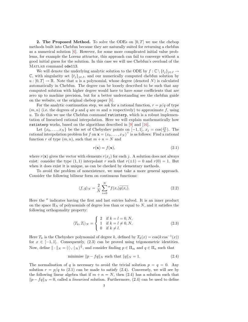
2. The Proposed Method. To solve the ODEs on [0, T ] we use the chebopmethods built into Chebfun because they are naturally suited for returning a chebfunas a numerical solution [6]. However, for some more complicated initial value prob-lems, for example the Lorenz attractor, this approach can fail to converge without agood initial guess for the solution. In this case we will use Chebfun’s overload of theMatlab command ode113.

We will denote the underlying analytic solution to the ODE by f : C \ {tj}j∈J →C, with singularity set {tj}j∈J , and our numerically computed chebfun solution byu : [0, T ] → R. Note that u is a polynomial, whose degree (denoted N) is calculatedautomatically in Chebfun. The degree can be loosely described to be such that anycomputed solution with higher degree would have to have some coefficients that arezero up to machine precision, but for a better understanding see the chebfun guideon the website, or the original chebop paper [6].

For the analytic continuation step, we ask for a rational function, r = p/q of type(m,n) (i.e. the degrees of p and q are m and n respectively) to approximate f , usingu. To do this we use the Chebfun command ratinterp, which is a robust implemen-tation of linearised rational interpolation. Here we will explain mathematically howratinterp works, based on the algorithms described in [9] and [16].

Let {x0, . . . , xN} be the set of Chebyshev points on [−1, 1], xj = cos( jπN ). The

rational interpolation problem for f on x = (x0, . . . , xN )> is as follows: Find a rationalfunction r of type (m,n), such that m + n = N and

r(x) = f(x), (2.1)

where r(x) gives the vector with elements r(xj) for each j. A solution does not alwaysexist: consider the type (1, 1) interpolant r such that r(±1) = 0 and r(0) = 1. Butwhen it does exist it is unique, as can be checked by elementary methods.

To avoid the problem of nonexistence, we must take a more general approach.Consider the following bilinear form on continuous functions:

〈f, g〉N =2N

N∑i=0

′′f(xi)g(xi). (2.2)

Here the ′′ indicates having the first and last entries halved. It is an inner producton the space ΠN of polynomials of degree less than or equal to N , and it satisfies thefollowing orthogonality property:

〈Tk, Tl〉N =

2 if k = l = 0, N,1 if k = l 6= 0, N,0 if k 6= l.

(2.3)

Here Tk is the Chebyshev polynomial of degree k, defined by Tk(x) = cos(k cos−1(x))for x ∈ [−1, 1]. Consequently, (2.3) can be proved using trigonometric identities.Now, define ‖ · ‖N = (〈·, ·〉N )

12 , and consider finding p ∈ Πm and q ∈ Πn such that

minimise ‖p− fq‖N such that ‖q‖N = 1. (2.4)

The normalisation of q is necessary to avoid the trivial solution p = q = 0. Anysolution r = p/q to (2.1) can be made to satisfy (2.4). Conversely, we will see bythe following linear algebra that if m + n = N , then (2.4) has a solution such that‖p− fq‖N = 0, called a linearised solution. Furthermore, (2.4) can be used to define

3

more general solutions in the case that n + m < N , called linearised least-squaressolutions for the rational interpolation problem [8]. The notion of a least-squaresproblem is a general one, in which the objective is to minimise a sum of squares.

Now we will see why the specific bilinear form was chosen. Let a = (a0, . . . , aN )>

and b = (b0, . . . , bN )> define polynomials p and q as follows:

p(x) =N∑

j=0

′′akTk(x), q(x) =N∑

j=0

′′bkTk(x). (2.5)

Then ‖p‖N = ‖a‖2, ‖q‖N = ‖b‖2 and so any linear problem in the values of p

and q can be restated as a linear problem in a and b. The transformation fromcoefficient space to value space can be stated as p(x) = CI ′′a, and q(x) = CI ′′bwhere C = (Tj(xi))N

i,j=0, and I ′′ is the identity matrix with the top-left and bottom-right entries halved. By the orthogonality relation (2.3), 2

N C>I ′′CI ′′ = I and so ifp(x) = (f · q)(x) then we have

a =2N

C>I ′′CI ′′a =2N

C>I ′′FCI ′′b, (2.6)

where F is diagonal matrix with diagonal entries f(x).Now let a and b be vectors containing the first m + 1 and n + 1 rows of a and b

respectively, and let a and b be vectors containing the last N − m and N − n rowsof a and b respectively. Let q ∈ Πn be the truncation of q ∈ ΠN (i.e. set b = 0) andsuppose that p and q solve the linearised least squares problem (2.4). Then since bydefinition of ‖ · ‖N we have

‖p− fq‖N = ‖p− p‖N , (2.7)

where p ∈ ΠN interpolates f · q, minimality implies that p must be the truncation ofp (i.e. a = 0 for p). Therefore, we have ‖p− fq‖N = ‖a‖2.

Now define Z = 2N C>I ′′FCI ′′, Z to be the matrix consisting of the first n + 1

columns and last N − m rows of Z, and Z to be the matrix consisting of the firstn + 1 columns and first m + 1 rows of Z. Then we have that

a = Zb, a = Zb, a = Zb. (2.8)

Minimality of ‖a‖2 over all q ∈ Πn implies that b must be made to minimise ‖Zb‖2.Therefore, in order for a and b to be a solution for (2.4) it suffices to take b tominimise ‖Zb‖2, then set a = Zb. The residual ‖p− fq‖N is exactly ‖Zb‖2.

If n + m = N , then Z is an n × (n + 1) matrix, so has a non-zero kernel. Hencethere exists a vector b with ‖Zb‖2 = 0, and the associated polynomials p and qexactly solve the linearised rational interpolation problem.

In the general case where n+m ≤ N , we can use the Singular Value Decomposition(SVD [20]) of Z to find the minimal singular value σmin of Z and associated singularvector b such that σmin = ‖Zb‖2, and indeed this is how ratinterp solves thelinearised least squares problem (2.4). For a matrix A ∈ Rm×n, its singular valuedecomposition is

A = UΣV >, (2.9)

where U is an m × m orthogonal matrix whose columns are eigenvectors of AA>, Vis an n × n orthogonal matrix whose columns are eigenvectors of A>A, and Σ is an

4

m×n diagonal matrix, whose diagonal entries are the square roots of the eigenvaluesof A>A or AA>, whichever is the smaller set. These diagonal entries are called thesingular values of A, and we take the decomposition so that they are ordered fromleft to right in Σ, greatest (σmax) to smallest (σmin). By expanding x in the orderedorthonormal basis {v1, . . . , vn} consisting of the columns of V , we see that ‖Ax‖2

achieves its maximum σmax at x = v1 and its minimum σmin at x = vn. Matlab hasthe command svd for its computation.

Noting that Tj(xi) = cos( ijπN ), multiplication by CI ′′ and 2

N C>I ′′ can be inter-preted as taking the discrete cosine transform (DCT) and inverse discrete cosine trans-form (iDCT) respectively. The Fast Fourier Transform (FFT) is used by ratinterpto efficiently compute the DCT and iDCT when computing Z.

This is not the end of the story because we have not discussed uniqueness. Ifthe minimal singular value σmin is multiple, of multiplicity d, say, then there exist dlinearly independent vectors b such that ‖Zb‖2 = σmin, corresponding to d differentpolynomials q. This case corresponds to p and q potentially sharing d roots. Inexact arithmetic these will cancel, but on a computer they almost certainly will not,producing a zero-pole pair known as a Froissart doublet.

By taking an appropriate linear combination, there exists a b with the last d− 1entries zero, corresponding to a q ∈ Πn−(d−1). From a robustness point of view, itis better to take this b because it will reduce the number of poles in r, reducing thechance of a Froissart doublet. It would be possible to use linear algebra to find thisb, but it is simpler to reduce n by d − 1 (keeping N and m the same) and startthe procedure again. This process can be repeated, giving the algorithm a uniquesolution.

This idea can be taken further to improve robustness when implemented on acomputer. The user sets a tolerance parameter tol, and if there are d singular valueswithin tol of σmin, then n is decreased by d − 1. The resulting p and q have theirdegrees reduced even further by discarding the higher coefficients smaller than tol inabsolute value.

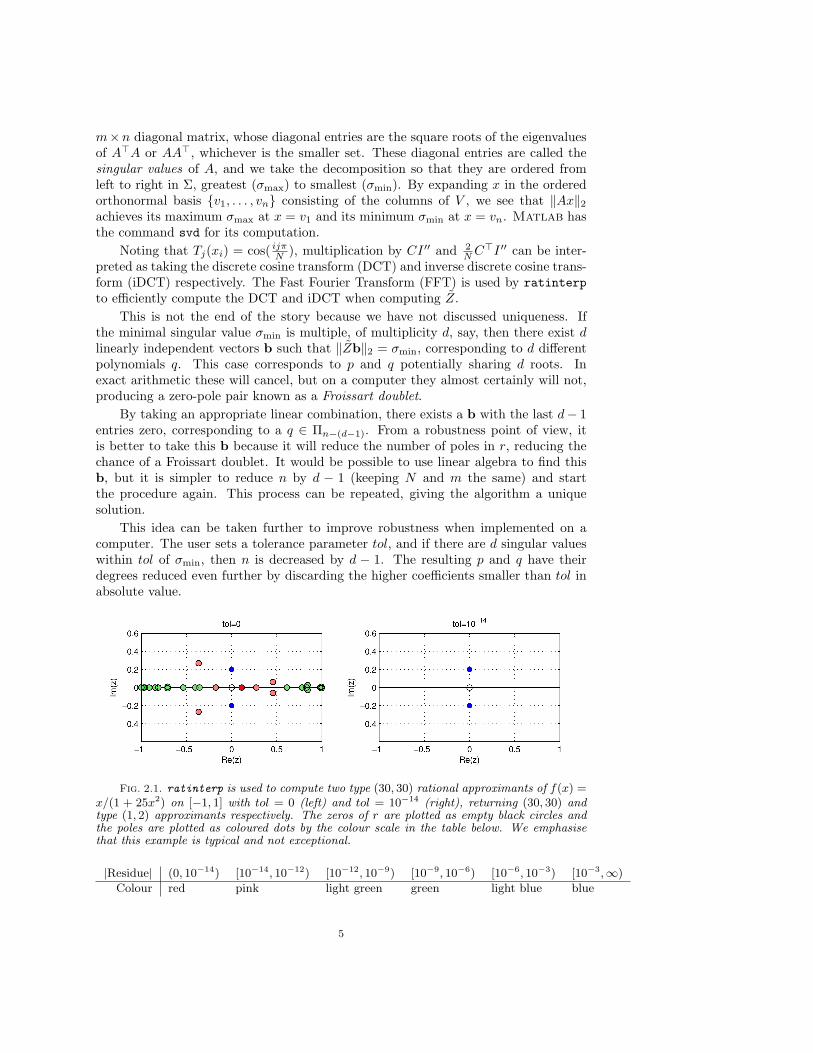
Fig. 2.1. ratinterp is used to compute two type (30, 30) rational approximants of f(x) =x/(1 + 25x2) on [−1, 1] with tol = 0 (left) and tol = 10−14 (right), returning (30, 30) andtype (1, 2) approximants respectively. The zeros of r are plotted as empty black circles andthe poles are plotted as coloured dots by the colour scale in the table below. We emphasisethat this example is typical and not exceptional.

|Residue| (0, 10−14) [10−14, 10−12) [10−12, 10−9) [10−9, 10−6) [10−6, 10−3) [10−3,∞)

Colour red pink light green green light blue blue

5

The tolerance parameter is by default 10−14, which in practice works well whenapproximating functions accurate to machine precision (around 10−16), but if youknow that f contains noise of magnitude ε, then tol = 100ε is a good suggestion forthe tolerance. If the tolerance is set at a value smaller than this, then ratinterpwill futilely use this noise for its approximation. We will use tol = 10−12 since u iscomputed numerically as the solution to an ODE and will therefore not be accurate tomachine precision: there will be noise in u with magnitude between 10−13 and 10−12.

In Figure 2.1, the plotted results follow the style of [9] where the poles are coloureddots with their colour decided by their residue according to the table below. Noticethe appearance of Froissart doublets when tol = 0, where coloured dots (poles) havean empty black circle (zero) in (almost) the same place.

The ratinterp algorithm delivers a rational function of type (µ, ν) where 0 ≤µ ≤ m, 0 ≤ ν ≤ n. We take the roots of q to approximate the singularities of f .ratinterp can also calculate the residues of the poles, which is implemented usingMatlab’s residue command [5].

Chebfun’s ratinterp is not restricted to using the Chebyshev points on [−1, 1]for the nodes. The method explained above generalises to arbitrary points in thecomplex plane, and the user can specify whatever nodes they want ratinterp to use.The general approach for the linearised interpolation problem is discussed in [16].The case where the nodes are the Nth roots of unity is particularly elegant becausethe polynomials satisfying a discrete orthogonality relation are simply the monomials(powers of roots of unity make up the Fourier basis). The linearised least squaresproblem and robustness steps for the case of roots of unity can be found in [9].

As well as the rational approximant of u, we can compute the Chebfun ellipseassociated with the chebfun u. The Chebfun ellipse is the Bernstein ellipse with ρparameter such that ρN = ε where ε is machine precision (approximately 10−16).This ellipse is a good estimate for the Bernstein ellipse associated with f , discussed inSection 1 [19, Ch.8]. This estimate is useful because at least one singularity of f lieson the edge of the Bernstein ellipse and poles deep inside the ellipse must be spurious.

Recall that we denote the degree of the chebfun solution to the ODE problem uby N , and this integer is computed automatically by Chebfun. Using few than N + 1nodes for our rational approximation would not be utilising all the information wehave about u, and using more than N + 1 nodes would be approximating data thathas been interpolated from N + 1 nodes anyway. Therefore we perform our rationalapproximation on N + 1 nodes if we are approximating a chebfun of degree N .

In summary, we perform the following list of operations as our proposed method:Solve the ODE problem using chebops or ode113 on [0, T ], producing a chebfun u ofdegree N ; compute a rational interpolant r = p/q from u on N + 1 Chebyshev pointsin [0, T ]; compute the locations of the poles by finding the roots of q and computetheir residues using residue; and compute the Chebfun ellipse associated for u toestimate the Bernstein ellipse for f .

3. Preliminary Experiments. A key question to ask when computing rationalapproximants is, what are good choices for m and n? This turns out to be rathertroublesome. The following quote is from Pade Approximants by G.A. Baker andP.R. Graves-Morris [1].

“In practice, whether one expects them or not, defects occur for allbut the simplest functions.”

Here, defect is synonymous with the spurious poles mentioned in the previous section.Baker and Graves-Morris are referring to Pade approximants rather than the rational

6

interpolation and least-squares approximants considered in this paper, but the prin-ciple still applies (see Figure 2.1). For the case of robust rational interpolation onthe unit circle, this issue is discussed in [9, sections 4 and 6]. For this project, theauthor performed some preliminary experiments with robust rational least-squaresapproximation on an interval.

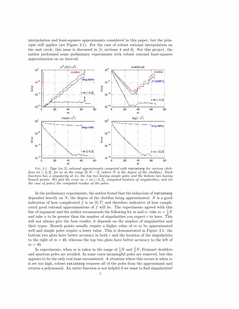
Fig. 3.1. Type (m, 2) rational approximants computed with ratinterp for various cheb-funs on [−2, 2], for m in the range [0, N − 2] (where N is the degree of the chebfun). Eachfunction has a singularity at ±i, the top two having simple poles and the bottom two havingbranch points. We plot the error in: r on [−2, 2], computed location of singularities, and (inthe case of poles) the computed residue at the poles.

In the preliminary experiments, the author found that the behaviour of ratinterpdepended heavily on N , the degree of the chebfun being approximated. N is a goodindication of how complicated f is on [0, T ] and therefore indicative of how compli-cated good rational approximations of f will be. The experiments agreed with thisline of argument and the author recommends the following for m and n: take m = 1

2Nand take n to be greater than the number of singularities you expect r to have. Thiswill not always give the best results; it depends on the number of singularities andtheir types. Branch points usually require a higher value of m to be approximatedwell and simple poles require a lower value. This is demonstrated in Figure 3.1: thebottom two plots have better accuracy in both r and the location of the singularitiesto the right of m = 40, whereas the top two plots have better accuracy to the left ofm = 40.

In experiments, when m is taken in the range of 13N and 2

3N , Froissart doubletsand spurious poles are avoided. In some cases meaningful poles are removed, but thisappears to be the only real issue encountered. A situation where this occurs is when mis set too high, robust ratinterp removes all of the poles from the approximant andreturns a polynomial. An entire function is not helpful if we want to find singularities!

7

We see this in all four of the plots in Figure 3.1, because the red and blue lines, whichrely on the existence of singularities, do not extend as far as the black lines, whichonly rely on the existence of a rational approximant.

Ideally, we would state and prove theorems that explain results such as thoseillustrated in Figure 3.1, but at present, little is understood about the robust least-squares algorithm. Can the relationship between the SVD of the linearised problemand the singularities of the resulting rational approximant be made precise? A morespecific question is how high m must be for the robust algorithm to remove all ofthe poles from the approximant. The rest of this article is an investigation into whatratinterp is capable of for the computation of singularities of differential equations,as a first step towards the required understanding.

4. ODEs under Investigation. This is the main section of the paper. Here wediscuss some specific ODEs with results showing computations of complex singularitiesfor their solutions. The first two examples are ones with straightforward explicitsolutions, and the last three are some examples from applied mathematics that areinteresting in their own right.

4.1. Simple Poles. The following nonlinear ODE (with appropriate boundaryconditions) has solution tanh(α + βx) for arbitrary constants α, β:

d2f

dx2+ 2βf

df

dx= 0. (4.1)

We used Chebfun to solve (4.1) with α = 0, β = 1 on the domain [−5, 5] andboundary conditions f(±5) = tanh(±5). The numerically computed solution u isa chebfun of degree N = 105, so following the strategy described in the previoustwo sections we used ratinterp to generate a type (b 1

2Nc, 10) = (52, 10) rationalapproximant r on the 106 Chebyshev points in [−5, 5]. ratinterp returned a type(31, 2) approximant which appears in Figures 4.1 and 4.2.

Table 4.1Error Data for Rational Approximation of tanh(z)

Quantity Max Error Mean Erroru on [−5, 5] 1.0× 10−12 2.0× 10−13

r on [−5, 5] 7.1× 10−12 1.4× 10−12

poles(r) 4.0× 10−8 4.0× 10−8

residues(r) 2.4× 10−7 2.4× 10−7

When f(x) = tanh(x) is extended into the complex plane it has simple poles at(2j +1)π

2 i for each j ∈ Z, each with residue 1. In Figure 4.1 and Table 4.1 we can seethat just using our heuristic from Section 3 for the values of m and n, we get fairlyaccurate results for the locations of the poles and residues. If one decreases m, r canapproximate the zeros at ±πi and even the poles further out at ± 3π

2 i, but accuracyof the approximation on [−5, 5] is sacrificed.

In Figure 4.2, bottom right, we can see that the rational approximation is onlyaccurate in a small oval around the interval, a barrier beyond which r blows uppolynomially (of very high degree). Nonetheless, if we are only interested in thenearest singularities to the real line this small window of meaningful continuation issatisfactory. The same cannot be said for the chebfun u, which blows up quicklyoutside of the Bernstein ellipse (bottom left).

8

Fig. 4.1. Schematic of the numerical analytic continuation of the solution to (4.1) on[−5, 5], showing simple poles at ±π

2i (blue dots) and a zero at 0 (circle). The Chebfun ellipse,

computed by Chebfun, is slightly larger than the actual Bernstein ellipse associated with tanh.

Fig. 4.2. Contour plots of the absolute value of tanh(z) (top), the chebfun numericalsolution to (4.1) u (left) and its ratinterp approximant r (right). The contours are colouredfrom blue to red on [0, 5]. The chebfun u is useless as an approximation of tanh(z) outsideof the Bernstein ellipse whereas the ratinterp approximant r reaches much further.

4.2. Logarithmic Branch Points. The following example is a first order ODEwith solution f(t) = log(1+(t−γ)2) for an arbitrary constant γ (given an appropriateinitial value):

df

dt+ 2(γ − t) exp(−f) = 0. (4.2)

9

The exponential term in (4.2) may seem contrived, but an example from combustiontheory, the time independent Frank-Kamenetskii blowup equation, takes a similarform: d2f/dx2 + A exp(f) = 0 [17].

Fig. 4.3. 3D plot of the absolute value of f(z) = log(1 + (z − 6)2) on [0, 10]× [−6, 6] ⊆C. The plot is coloured by argument ranging from −π to π. We can clearly see the twologarithmic singularities and the branch cuts behind them, across which the argument of f isdiscontinuous.

We consider the case γ = 6, for which we have plotted the surface generated bythe absolute value of the analytical solution. The surface is coloured by the argumentof the complex value in order to see that along the branch cuts the solution is notcontinuous. We solved (4.2) using chebops on the interval [0, 10] with initial dataf(0) = log(37). The solution u has degree N = 137 so as in the previous example, weused this information and computed a type (b 1

2Nc, 10) = (68, 10) rational approxi-mant r on 138 Chebyshev points in [0, 10]. ratinterp returned a type (57, 4) rationalfunction with poles at t = 6.0017± 1.0429i, 6.0109± 1.2515i.

This is typical of rational approximants; in practice branch cuts are approximatedby lines of poles in the rational function as in Figure 4.4 and the actual location ofthe branch point itself is not very accurate (see Table 4.2).

Table 4.2Error data for rational approximation of the solution to (4.2). The error in the location

of the branch points (poles(r)) is much worse than that for the poles in the previous example.

Quantity Max Error Mean Erroru on [0, 10] 3.7× 10−12 1.1× 10−12

r on [0, 10] 1.9× 10−9 2.0× 10−10

poles(r) 4.3× 10−2 4.3× 10−2

What relevance do the residues of the poles of r have for f at branch pointsingularities? For this example the poles of r have residues of absolute value 1.3×1014

10

Fig. 4.4. Top: Schematic of the poles (blue dots) and roots (circles) of the ratinterpapproximant of the numerical solution to (4.2) on [0, 10]. Middle: Contour plot of the ab-solute value of the underlying solution log(1 + (z − 6)2). Left: polynomial approximationof the solution to (4.2), which blows up outside of its Bernstein ellipse. Right: ratinterpapproximant r which approximates the solution further into the complex plane. The contoursare coloured blue to red on [0, 5].

and 1.4×1014, which are surprisingly large. This could be a feature of our method forcalculating the residues, Matlab’s residue command [5]. The documentation warnsthat the method is unstable in some circumstances. It could also be a property of therational interpolation and least squares approximation for branch point singularities.

4.3. Lorenz Attractor. Viswanath and Sahutoglu 2010 [21] is a fascinatingpaper, which puts forward the point of view that although the Lorenz attractor isa well known example in applied mathematics, relatively little is known about themathematical analysis of its solutions. The authors present an analytic treatmentwhere they consider time as a complex variable and show that a certain class ofsolutions respresented by so-called Ψ-series are singular, with complex logarithmicsingularities close to the real line.

The system was originally studied by Lorenz, who derived it from the simplified11

equations of convection rolls arising models of the atmosphere:

dx

dt= 10(y − x),

dy

dt= 28x− y − xz,

dz

dt= −8z/3 + xy.

(4.3)

It is an early example of a chaotic dynamical system, in which small changes in initialdata can produce wildly different results in the solution. Lorenz used this in his 1963paper to argue that accurate long-range weather prediction may be impossible [12].

Definition 4.1. A logarithmic Ψ-series centered at t0 is a series of the form

∞∑j=−J

Pj(η)(t− t0)j , η = log(b(t− t0)), (4.4)

where J is an integer, Pj is a polynomial and b is a complex number with |b| = 1.We can take b = ±i without loss of generality. As t → t0 a Ψ-series behaves

asymptotically like a pole of Jth order, as the polynomials in η are “overpowered” bythe (t− t0)−J term (Hille calls them pseudopoles [10]). We expect pseudopoles to beapproximated well by rational functions because of this asymptotic approximation.

Ψ-series solutions of the Lorenz attractor described in [21] are of the form

x(t) =P−1(η)t− t0

+ P0(η) + P1(η)(t− t0) + P2(t− t0)2 + . . . ,

y(t) =Q−2(η)(t− t0)2

+Q−1(η)t− t0

+ Q0(η) + Q1(η)(t− t0) + Q2(t− t0)2 + . . . ,

z(t) =R−2(η)(t− t0)2

+R−1(η)t− t0

+ R0(η) + R1(η)(t− t0) + R2(t− t0)2 + . . . ,

(4.5)

in the disc |t− t0| ≤ r for some r > 0 but with the singular point t = t0 and a branchcut deleted from the disc. It should be borne in mind that it has not yet been provedthat all singular solutions of the Lorenz attractor take this form.

The chebop methods in Chebfun struggle to solve the Lorenz system without agood initial starting point as it is nonlinear and highly oscillatory, so we use Chebfun’soverload of ode113. The same applies to examples in subsections 4.4 and 4.5. Forthis experiment we set our initial conditions to be

x(0) = −14, y(0) = −15, z(0) = 20, (4.6)

which gives the beautiful butterfly shaped trajectory in 3-dimensional space shown inthe second plot in Figure 4.5. We solved the Lorenz system on [0, 5] with the aboveinitial conditions, and ode113 returned three chebfuns ux, uy and uz with degreesNx = 462, Ny = 509 and Nz = 498. We used our general strategy and computedrational approximants of types (231, 20), (255, 20) and (249, 20) and ratinterp re-turned rational functions of types (173, 10), (227, 10) and (221, 10) respectively.

We can see from (4.5) that x, y and z have precisely the same singularities, t0,so we should expect our rational approximants rx, ry and rz to have the same singu-larities (assuming the initial conditions give a solution of this Ψ-series form). Table4.3 lists the locations of the 10 computed singularities for each component and we do

12

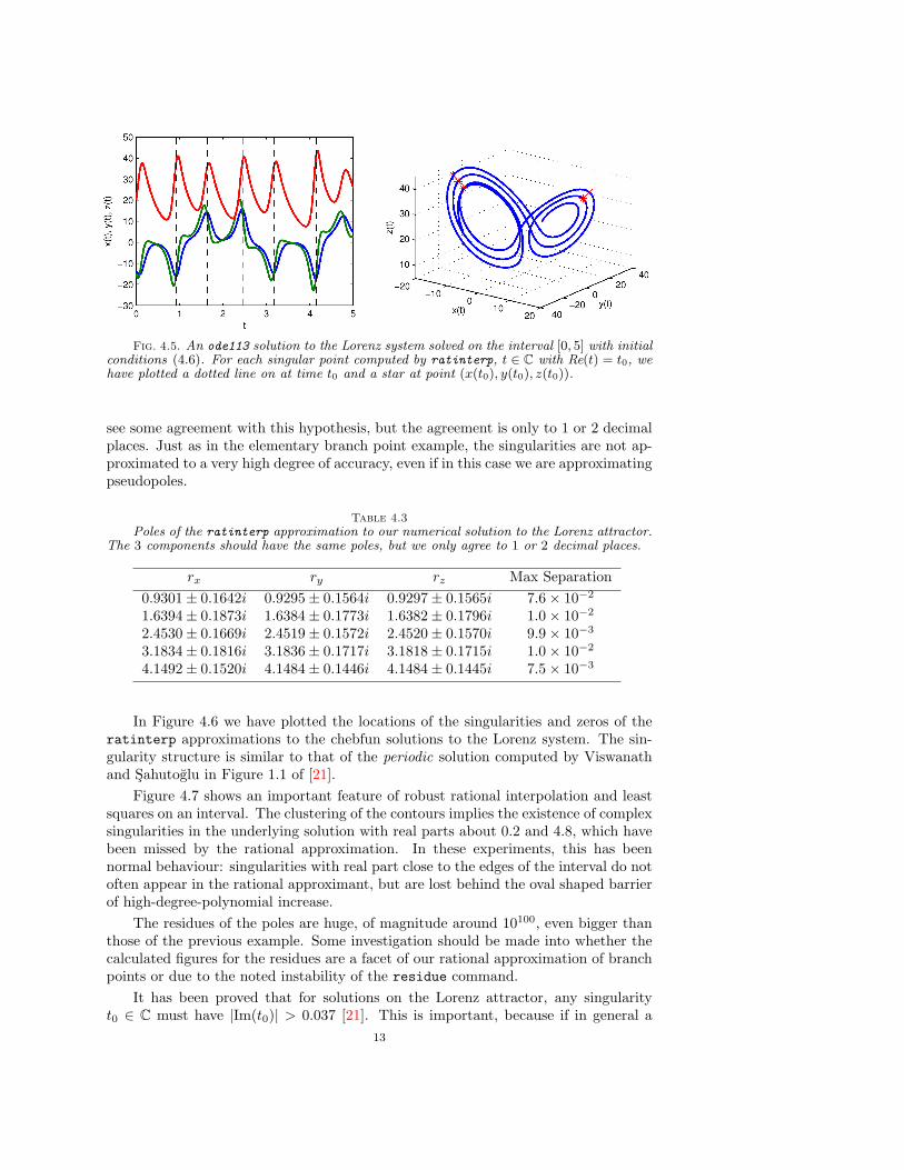
Fig. 4.5. An ode113 solution to the Lorenz system solved on the interval [0, 5] with initialconditions (4.6). For each singular point computed by ratinterp, t ∈ C with Re(t) = t0, wehave plotted a dotted line on at time t0 and a star at point (x(t0), y(t0), z(t0)).

see some agreement with this hypothesis, but the agreement is only to 1 or 2 decimalplaces. Just as in the elementary branch point example, the singularities are not ap-proximated to a very high degree of accuracy, even if in this case we are approximatingpseudopoles.

Table 4.3Poles of the ratinterp approximation to our numerical solution to the Lorenz attractor.

The 3 components should have the same poles, but we only agree to 1 or 2 decimal places.

rx ry rz Max Separation0.9301± 0.1642i 0.9295± 0.1564i 0.9297± 0.1565i 7.6× 10−2

1.6394± 0.1873i 1.6384± 0.1773i 1.6382± 0.1796i 1.0× 10−2

2.4530± 0.1669i 2.4519± 0.1572i 2.4520± 0.1570i 9.9× 10−3

3.1834± 0.1816i 3.1836± 0.1717i 3.1818± 0.1715i 1.0× 10−2

4.1492± 0.1520i 4.1484± 0.1446i 4.1484± 0.1445i 7.5× 10−3

In Figure 4.6 we have plotted the locations of the singularities and zeros of theratinterp approximations to the chebfun solutions to the Lorenz system. The sin-gularity structure is similar to that of the periodic solution computed by Viswanathand Sahutoglu in Figure 1.1 of [21].

Figure 4.7 shows an important feature of robust rational interpolation and leastsquares on an interval. The clustering of the contours implies the existence of complexsingularities in the underlying solution with real parts about 0.2 and 4.8, which havebeen missed by the rational approximation. In these experiments, this has beennormal behaviour: singularities with real part close to the edges of the interval do notoften appear in the rational approximant, but are lost behind the oval shaped barrierof high-degree-polynomial increase.

The residues of the poles are huge, of magnitude around 10100, even bigger thanthose of the previous example. Some investigation should be made into whether thecalculated figures for the residues are a facet of our rational approximation of branchpoints or due to the noted instability of the residue command.

It has been proved that for solutions on the Lorenz attractor, any singularityt0 ∈ C must have |Im(t0)| > 0.037 [21]. This is important, because if in general a

13

Fig. 4.6. A schematic of the rational approximation of ux (blue), uy (green) and uz (red)of the ode113 solution to (4.3) on [0, 5]. The singularity structure is similar to that of theperiodic solution computed by Viswanath and Sahutoglu in Figure 1.1 of [21].

Fig. 4.7. A contour plot of the absolute value of the ratinterp approximant rx(t) of thenumerical solution to the Lorenz attractor (4.3). The contours are coloured blue to red on[0, 80]

solution to a differential equation satisfies |Im(t0)| > τ , the transformation

ζ =exp(πt/2τ)− 1exp(πt/2τ) + 1

(4.7)

maps the strip where the solution is analytic to the unit disc. The solution musttherefore have a globally convergent expansion in powers of ζ. Numerical experimentssuch as the ones we have done here, and those done by Viswanath and Sahutoglu

14

for [21] can help inform the analysis in this fashion.

4.4. Lotka-Volterra Predator-Prey Model. Our next example is from math-ematical ecology. A simple population model for interacting species is the Lotka-Volterra predator-prey model

dx

dt= αx− βxy,

dy

dt= −γy + δxy,

(4.8)

where α, β, γ, δ are positive constants with γ < β. In the model, y represents thepopulation of a predator and x represents the population of its prey as they varyover time [11]. The coefficient α encodes the rate of reproduction in prey irrespectiveof predators, β describes the rate at which predators kill the prey, γ represents thestarvation of predators in the absence of prey, and δ expresses the rate at whichpredators reproduce given enough prey to feed on.

If we restrict ourselves to the physically meaningful case where x, y > 0, thesystem can be integrated exactly. Dividing the two equations and using the chainrule gives the separable equation,

δx− γ

x

dx

dy=

α− βy

y, (4.9)

and we obtain an implicit solution by integrating with respect to y:

H = (α log y − βy) + (γ log x− δx). (4.10)

H can be considered as the first integral, Hamiltonian or energy of the system and isa constant that depends only on the initial conditions. We plot this trajectory (x, y)in Figure 4.9 for different values of H. The parameters and initial conditions we usehere are α = β = 0.5, γ = δ = 1, x(0) = 2, y(0) = 3.

There are still many open problems for the analysis of the Lorenz attractor, whichis a three-dimensional autonomous system [21]. In contrast, the analysis of the Lotka-Volterra system, a plane autonomous system, is further developed. Hille proved thatthe plane quadratic system

dx

dt= x(a0 + a1x + a2y), (4.11)

dy

dt= y(b0 + b1x + b2y), (4.12)

has a logarithmic Ψ-series singularity of order 1 (i.e. J = 1 in the expression (4.4))if (a1 − b1)(a2 − b2)/(a1b2 − a2b1) is a positive integer [10, Sec. 12.5,12.6]. For theLotka-Volterra system, we have

(a1 − b1)(a2 − b2)a1b2 − a2b1

=(0− δ)(−β − 0)0 · 0− (−β)(δ)

= 1. (4.13)

Hence the Lotka-Volterra system always has a simple logarithmic Ψ-series singularityin the complex plane.

As in the previous subsection, we used ode113 to solve the Lotka-Volterra systemon [0, 45], which returned two chebfuns u and v with degrees Nx = 743 and Ny = 737.

15

Fig. 4.8. ode113 solutions u and v to (4.8) with α = β = 0.5, γ = δ = 1, u(0) = 2, v(0) =3 in blue and green respectively.

Fig. 4.9. Left: Implicit solutions to (4.8) with α = β = 0.5, γ = δ = 1, for various valuesof H. Right: A numerically computed trajectory for the same problem with initial conditionsu(0) = 2, v(0) = 3. The point on the trajectory corresponding to u and v at the time that isthe real part of the (periodic) complex singularities has been marked ((u, v) = (3.44, 2.27)).

Table 4.4Singularities of the Lotka-Volterra equations for α = β = 0.5, γ = δ = 1. They should,

by periodicity, have the same imaginary part, but we can see that the accuracy in this respectis quite low.

rx ry Separation11.0204± 0.9166i 11.0244± 0.9170i 4.0× 10−3

22.3637± 0.9169i 22.3692± 0.9171i 5.5× 10−3

33.7086± 0.9168i 33.7128± 0.9168i 4.2× 10−3

For the benefit of the reader, these two chebfuns have been plotted in Figure 4.8.Following the heuristics discussed in Section 3, we used ratinterp with target types(371, 20) and (366, 20) on 372 and 366 Chebyshev points in [0, 45], which returnedrational approximants of types (297, 6) and (287, 6).

In Figure 4.10, we see that the periodicity of the solution is expressed somewhatin the rational approximant, but the appoximant still blows up outside of an ovalshaped barrier. What should plainly be singularities just off the real line near time 0and time 45 are lost behind the barrier, just as in the Lorenz attractor example. Toapproximate these singularities, can solve the system on [−15, 15] and [30, 60].

Although the user can see where the barrier is by inspection, and that there maybe further singularities behind it, if an automated procedure for locating singularities

16

Fig. 4.10. We solved the Lotka-Volterra system on the interval [0, 45] using ode113.These are contour plots of rational approximants rx(t) (top) and ry(t) (bottom) to the nu-merical solution, in the complex t-plane. We can see the periodic nature of the solutions inthe complex plane, with period around 11.3, and the branch cut associated with each singular-ity, the beginnings of which protrude outwards from the real line. The contours are colouredblue to red on [0, 20]

is what we desire, estimates for the size and shape of the oval barrier for the rationalapproximant would be necessary.

4.5. Three-Body Problem. The three-body problem is the term used to referto the system of ODEs modelling the motion of three points of prescribed massesunder mutual Newtonian gravitation in three dimensions:

d2x1

dt2= m2

x2 − x1

‖x2 − x1‖3+ m3

x3 − x1

‖x3 − x1‖3,

d2x2

dt2= m1

x1 − x2

‖x1 − x2‖3+ m3

x3 − x2

‖x3 − x2‖3,

d2x3

dt2= m1

x1 − x3

‖x1 − x3‖3+ m2

x2 − x3

‖x2 − x3‖3.

(4.14)

Here x1, x2 and x3 are the positions of three particles with masses m1, m2 and m3

respectively, in space at time t ∈ R. The problem is a classic that has fascinatedsome of the greatest mathematicians: Newton, Euler, Lagrange, Laplace, Poincareand even those of today.

In 2000 Chenciner and Montgomery published a paper proving the existence of a“remarkable periodic solution to the three-body problem in the case of equal masses”

17

[4], where the three particles travel around in a planar figure of eight shape as inFigure 4.11. This particular solution was first discovered numerically by C. Moorein 1993 [14]. Such solutions to the general n-body problem with smooth periodictrajectories have since been called choreographies and it is now an active area ofresearch [13].

Fig. 4.11. The paths of the three complex-valued bodies x1, x2 and x3 solving (4.14) travelperiodically in a figure of eight shape in the complex plane. We colour the bodies and theirpaths for the first third of their periods here in blue, green and red respectively.

Since this special case of the three-body problem is planar, we can use complexarithmetic to represent the positions x1, x2 and x3

1. Without loss of generality wemay assume the masses are all equal to 1. The initial conditions for the figure of eightare given in the paper (computed by Carles Simo) and are as follows:

x1 = −x2 = 0.97000436− 0.24308753i, x3 = 0,

x1 = x2 = 0.466203685 + 0.43236573i, x3 = −0.93240737− 0.86473146i,(4.15)

The resulting choreography has period T = 6.32591398 (approx.), so we used ode113to solve the system on the interval [0, 12.65182796] (two periods) which returnedu1, u2 and u3, chebfuns of degree 330, 330 and 335 respectively. We used ratinterpto compute type (165, 20), (165, 20), and 167, 20) rational approximations on 331, 331and 336 Chebyshev points on the interval, which returned rational functions r1, r2

and r3 of types (157, 7), (157, 7) and (159, 6).The resulting singularity structure shown in Figure 4.12 is different from all the

other examples: Because x1, x2 and x3 are complex valued, the singularities do notnecessarily come in conjugate pairs. Now, let us turn to the complex t-plane (as op-posed to the complex xi plane) on which the solution should be T -periodic throughoutand let us assume that x3 has a singularity at complex time t = αT + βi. Our argu-ment will be simplest if we use x3 because its initial position is the origin. It followsfrom the four-fold symmetry of the solution that x3 is singular for values of t with realparts: ±αT, T/2 ± αT (modulo T ), and imaginary part ±β. This is precisely whatwe see in our numerical analytic continuation (see Figure 4.12 and Table 4.5), foursingularities for each body per period, with two bodies participating in each.

1To be clear, each body xi takes complex values in a figure eight shape for real time t, but wealso consider complex time, at which xi can take any value in the complex plane

18

Fig. 4.12. Contour plots of the figure-of-eight solution solved using ode113 on the timeinterval [0, 12.6518], extended into the complex plane using rational interpolation. Each reddot is a singularity in the system for complex time, with two bodies participating in each.The contours are coloured from blue to red on the interval [0, 2]

Now, by construction the particles divide the circuit into three by time, sox1 (t) = x2 (t + T/3) = x3 (t + 2T/3). Therefore if x3 and x2 (or x1) participate in thesingularity at αT , x3 also has a singularity with real part αT − T/3 (or αT − 2T/3).

We can use these two symmetrical observations to find equations involving αmodulo T ; solving for α, we can find all possibilities for its numerical value. Forexample, αT +T/3 = T/2−αT implies α = 1/12. One finds that the only possibilitiesare α = 1/12, 5/12, 7/12, 11/12.

This gives us good reason to postulate that the real parts of the singularities ofthe figure of eight solution are (modulo T and to 4 decimal places),

αT =

1.5815, 2.6358, 4.7444, 5.7988 (for x1),0.5272, 1.5815, 3.6901, 4.7444 (for x2),0.5272, 2.6358, 3.6901, 5.7988 (for x3),

(4.16)

and our numerical results agree with this to 1 or 2 decimal places (see Table 4.5 andFigure 4.13). This is, as with the previous three examples, not very accurate, butnonetheless ratinterp did not produce any spurious poles.

The singularity structure of the figure of eight solution was brought to the author’sattention in a private communication with Divakar Viswanath, for which the authoris very grateful. The symmetry argument above for the possible locations of the

19

Table 4.5Singularities of three bodies for the figure-of-eight solution to the three body problem.

Two bodies participate in each singularity.

r1 r2 r3 Separation1.5776− 0.5735i 1.6141− 0.5387i 5.0× 10−2

2.6331 + 0.5447i 2.6309 + 0.5416i 3.8× 10−3

3.6898− 0.5511i 3.6886− 0.5484i 3.0× 10−3

4.7462 + 0.5518i 4.7440 + 0.5533i 2.7× 10−3

5.7981− 0.5532i 5.8002− 0.5527i 2.2× 10−3

6.8537 + 0.5532i 6.8516 + 0.5527i 2.2× 10−3

7.9078− 0.5533i 7.9057− 0.5518i 2.6× 10−3

8.9621 + 0.5511i 8.9633 + 0.5484i 3.9× 10−3

10.0187− 0.5447i 10.0210− 0.5416i 3.9× 10−3

11.0378 + 0.5387i 11.0743 + 0.5735i 5.0× 10−2

Fig. 4.13. The configuration of the particles at times t = 0.5272, 2.6358, 3.6901, 5.7988,the real parts of the singular points of x3. Coloured black is x3(t) with x1 and x2 shown asempty circles. The bodies form an isosceles triangle at these times.

singularities is due him as well.

5. Discussion.

5.1. Computing Complex Singularities of Differential Equations. Wehave performed numerical experiments using Chebfun’s ratinterp for computingcomplex singularities of solutions to some interesting ODE problems. We used astrategy developed in preliminary experiments and demonstrated that we can suc-cessfully find the singularities of difficult problems while avoiding spurious poles. Theclaim of Gonnet et al. [9], that the algorithm is robust, is evidently justified.

The robust algorithm ratinterp has potential for the numerical study of parabolicPDEs and parametrised problems, because implementation of our strategy allows thecomputation of the singularities at each time step or parameter variation to be au-tomated. It is however, not suitable for applications which require a high level ofaccuracy. As was pointed out in [9] the error in the rational approximant is increasedby the inclusion of the robustness procedure, dependent on the tol parameter. But

20

if ratinterp is used to reliably find the approximate locations of the singularities,other methods such as the method of steepest ascent can be used to find preciselocations [7].

5.2. Stability of Barycentric Interpolation Formulas for Extrapolation.During our experiments, we noticed a surprising instability. When ratinterp returnsthe rational approximant, if we use Chebyshev points, equispaced points around theunit circle or some other specific types of points, it returns a rational barycentricinterpolation formula. This is a formula of the form

r(x) =N∑

j=0

wjf(xj)x− xj

/ N∑j=0

wj

x− xj, wj =

q(xj)∏i 6=j(xi − xj)

, (5.1)

where f is the function we are approximating in the interpolation points, {xj} (whichthroughout this paper have been Chebyshev points on [a, b]). It is a tricky calculationto show that for Chebyshev points the weights are wj = (−1)jq(xj), after cancellingout factors independent of j, with w0 and wN equal to half this formula [2].

The instability arises for x outside of the Chebfun ellipse for f (defined in theSection 2), and is due to the following formula:

N∑j=0

wj

x− xj=

q(x)∏Ni=0(x− xi)

. (5.2)

As the absolute value of x increases, the right hand side of (5.2) decreases to machineprecision, beyond which it cannot decrease any further. The result is a dramatic lossof accuracy in (5.1) until there are no accurate digits at all. We can see in Figure 4.1for example, that a polynomial can be extrapolated throughout the Bernstein ellipse,but outside of that it is useless as an approximation of the underlying function, so ifwe cannot stably evaluate our rational approximant outside of the Bernstein ellipse weare doing no better than we can with a polynomial! More detail can be found in a shortarticle written with Trefethen and Gonnet [22]. ratinterp has since been correctedto evaluate the rational function as the quotient of two polynomials, each evaluatedby a numerically stable version of polynomial barycentric interpolation formula.

5.3. Further Work. There are some issues with the calculation of residues.In Gonnet et al.’s program ratdisk [9], the precursor to ratinterp, the residueis calculated using a trapezium rule approximation to the associated contour inte-gral. This turns out not to be very accurate for all but the simplest of functions.The method used in Chebfun’s ratinterp is implemented using Matlab’s residuefunction, which is much more accurate but represents an ill-posed problem; if thenumerator is close to a polynomial with multiple roots then small changes in the datacan make arbitrarily large changes in the resulting poles and residues [5].

We noted that the residues calculated in this way can be remarkably large, mostprobably because of this instability. A short study comparing different methods ofcalculating residues should be done to get to the bottom of the issue.

Gonnet, Guttel and Trefethen have produced a paper on a robust implementationof Pade approximation [8]. They achieve robustness using the SVD of a linearisedproblem, just as in the robust implementation of rational interpolation and leastsquares. The question of how the SVD of the linear system is related to the singulari-ties in the Pade approximant should be explored too, just as for rational interpolation,and their comparison could lead to a more concrete theory of these SVD-based robustalgorithms for rational approximation.

21

6. Acknowledgements. The author would like to thank Nick Trefethen forhis guidance and supervision during the project. His advice and suggestions wereinvaluable, especially when he took the time to read and comment on the early draftsof this paper. Many thanks to Andre Weideman for his insight and stimulatingdiscussion during his brief stay in the UK, Pedro Gonnet for his astounding expertise inscientific computing, Alex Townsend for the voice of reason in times of confusion, andeveryone at Oxford University in the Numerical Analysis Group for their hospitality,especially the administrator, Lotti Ekert. This paper was part of a summer researchproject funded by an EPSRC Undergraduate Vacation Bursary.

REFERENCES

[1] G.A. Baker and P.R. Graves-Morris, Pade approximants, vol. 59, Cambridge Univ. Press,1996.

[2] J.-P. Berrut and L.N. Trefethen, Barycentric lagrange interpolation, SIAM Review, 46(2004), pp. 501–517.

[3] F. Bornemann, P. Clarkson, P. Deift, A. Edelman, A. Its, and D. Lozier, Painleveproject on the web, Physics Today, 63 (2010), p. 10.

[4] A. Chenciner and R. Montgomery, A remarkable periodic solution of the three-body problemin the case of equal masses, Annals of Mathematics, Second Series, 152 (2000), pp. 881–902.

[5] MATLAB documentation, residue.[6] T.A. Driscoll, F. Bornemann, and L.N. Trefethen, The chebop system for automatic

solution of differential equations, BIT Numerical Mathematics, 48 (2008), pp. 701–723.[7] B. Fornberg and J.A.C. Weideman, A numerical methodology for the Painleve equations,

Journal of Computational Physics, (2011).[8] P. Gonnet, S. Guttel, and L.N. Trefethen, Robust Pade approximation via SVD, SIAM

Review, (2012).[9] P. Gonnet, R. Pachon, and L.N. Trefethen, Robust rational interpolation and least-squares,

Electronic Transactions on Numerical Analysis, 38 (2011), pp. 146–167.[10] E. Hille, Ordinary differential equations in the complex domain, Dover Publications, 1997.[11] F. Hoppensteadt, Lotka-Volterra equation, Scholarpedia.[12] E.N. Lorenz, Deterministic nonperiodic flow, Atmos. J. Sci., 20 (1963), pp. 130–141.[13] R. Montgomery, N-body choreographies, Scholarpedia.[14] C. Moore, Braids in classical dynamics, Physical Review Letters, 70 (1993), pp. 3675–3679.[15] R. Pachon, Algorithms for polynomial and rational approximation in the complex domain,

PhD thesis, University Of Oxford, 2010.[16] R. Pachon, P. Gonnet, and J. Van Deun, Fast and stable rational interpolation in roots of

unity and chebyshev points, SIAM Journal on Numerical Analysis, 50 (2012), pp. 1713–1734.

[17] L.N. Trefethen, PDE coffee table book: blow-up equation with exp(u) nonlinearity,http://people.maths.ox.ac.uk/trefethen/pdectb/blowup22.pdf.

[18] , Six myths of polynomial interpolation and quadrature, Mathematics Today, August(2011), pp. 184–188.

[19] , Approximation Theory and Approximation Practice, SIAM, 2012.[20] L.N. Trefethen and D. Bau, Numerical linear algebra, SIAM, 1997.[21] D. Viswanath and S. Sahutoglu, Complex singularities and the Lorenz attractor, SIAM

Review, 52 (2010), pp. 294–314.[22] M. Webb, L.N. Trefethen, and P. Gonnet, Stability of barycentric interpolation formulas

for extrapolation, SIAM J. Sci. Comput, (2012).[23] J.A.C. Weideman, Computing the dynamics of complex singularities of nonlinear PDEs, SIAM

J. Appl. Dyn. Syst, 2 (2003), pp. 171–186.

22