Variance Risk Premia∗

PETER CARR†

Bloomberg L.P. and Courant Institute

L IUREN WU‡

Zicklin School of Business, Baruch College

First draft: July 26, 2003

This version: February 25, 2004

Filename:VarianceSwap15.tex

∗We thank David Hait and OptionMetrics for providing the option data, Alex Mayus for clarifying trading practices,

Rui Yao for help on data processing, and Turan Bali, Mikhail Chernov,Robert Engle, Dilip Madan, Benjamin Wurzburger,

Jing Zhang, Chu Zhang, and seminar participants at Baruch College (CUNY) and Hong Kong University of Science and

Technology for comments and discussions. We assume full responsibility for any errors. We welcome comments, including

references we have inadvertently missed.†499 Park Avenue, New York, NY 10022; tel: (212) 893-5056; fax: (917) 369-5629;pcarr4@bloomberg.com.‡One Bernard Baruch Way, Box B10-225, New York, NY 10010; tel: (646) 312-3509; fax: (646) 312-3451;

Liuren Wu@baruch.cuny.edu; http://faculty.baruch.cuny.edu/lwu.

Variance Risk Premia

ABSTRACT

We propose a direct and robust method for quantifying the variance risk premium on financial

assets. We theoretically and numerically show that the risk-neutral expected value of the return

variance, also known as the variance swap rate, is well approximated by the value of a particular

portfolio of options. Ignoring the small approximation error, the difference between the realized

variance and this synthetic variance swap rate quantifies the variance risk premium. Using a large

options data set, we synthesize variance swap rates and investigate the historical behavior of vari-

ance risk premia on five stock indexes and 35 individual stocks.

JEL CLASSIFICATION CODES: G10, G12, G13, C51.

KEY WORDS: Stochastic volatility; variance risk premia; variance swap; volatility swap; option pric-

ing; expectation hypothesis; leverage effect.

Variance Risk Premia

The grant of the 2003 Nobel prize in economics has made available to the general public the well-

documented observation that return variances are random over time. Therefore, when investing in

a security such as a stock or a stock portfolio, an investor faces at leasttwo sources of uncertainty,

namely the uncertainty about the return as captured by the return variance, and the uncertainty about

the return variance itself.

It is important to know how investors deal with the uncertainty in return variance to effectively

manage risk and allocate assets, to accurately price and hedge derivative securities, and to understand

the behavior of financial asset prices in general. We develop a direct and robust method for quantifying

the return variance risk premium on an asset using the market prices of options written on this asset.

Our method uses the notion of a variance swap, which is an over-the-counter contract that pays the

difference between a standard estimate of the realized variance and the fixed swap rate. Since variance

swaps cost zero to enter, the variance swap rate represents the risk-neutral expected value of the realized

return variance. We theoretically and numerically show that the variance swap rate can be synthesized

accurately by a particular linear combination of option prices. Ignoring the small approximation error,

the difference between the ex-post realized variance and this synthetic variance swap rate quantifies the

variance risk premium. Using a large options data set, we synthesize variance swap rates and analyze

the historical behavior of variance risk premia on five stock indexes and 35 individual stocks.

If variance risk is not priced, the time series average of the realized return variance should equal the

variance swap rate. Otherwise, the difference between the expected value of the return variance under

the statistical probability measure and the variance swap rate reflects the magnitude of the variance risk

premium. Therefore, by comparing the variance swap rate to the ex-post realized return variance, we

can empirically investigate the behavior of the variance risk premium.

Widespread appreciation of the significance of variance risk by the practitioner community has

recently engendered the introduction of a slew of financial products with payoffs that are directly tied

to estimates of realized variance or volatility. Nowadays, variance and volatilityswaps trade actively

over the counter on major stocks, stock indexes, and currencies. In September of 2003, the Chicago

Board of Options Exchange (CBOE) redefined its well-known volatility index(VIX) in such a way that

1

it approximates the 30-day variance swap rate of the S&P 500 index return.In March 2004, futures on

this VIX will begin trading. These futures contracts represent a simple wayto trade variance realized

over a future time period. At the time of this writing, options on the VIX are also planned.

Despite the recent surge in liquidity in volatility contracts, high-quality historicaltime-series data

on variance swap rates are not yet available. In this paper, we circumvent this issue by synthesizing re-

turn variance swap rates. Working in complete generality, we show how the payoff of a return variance

swap can be accurately approximated theoretically by combining the payoff from a static position in

a continuum of European options with a dynamic trading strategy in the underlying futures. We show

that a sufficient condition for our replication strategy to be exact is that theunderlying asset’s return

dynamics are continuous over time. It is important to appreciate that no restrictive assumptions are

necessary on the dynamics followed by the return variance. In particular, the instantaneous variance

rate can jump and it need not even be observable. In this sense, the replicating strategy is robust.

When the underlying asset price can jump, the strategy fails to replicate perfectly. We show that the

instantaneous approximation error is third order in the size of the jump. When applying the theoretical

relation in practice, we also introduce an approximation error due to the interpolation and extrapolation

needed to generate the required continuum of option prices from the finite number of available option

quotes. We numerically show that both sources of approximation errors are small under realistic price

processes and market settings.

Variance swaps are not the only volatility derivatives that can be robustlyreplicated. Carr and Lee

(2003a) develop robust replicating strategies for any contracts with terminal payoffs that are functions

of the realized variance and final price. In particular, they develop the replicating strategy for a volatility

swap, the payoff of which is linear in the square root of the realized variance. They argue that the Black

and Scholes (1973) at-the-money implied volatility is an accurate approximation of the volatility swap

rate. We numerically confirm the accuracy of their theoretical arguments. We conclude that variance

swap rates and volatility swap rates can both be accurately approximated using market prices of options

and their underlying assets.

Given these conclusions, we synthesize variance and volatility swap ratesusing options data on five

of the most actively traded stock indexes and 35 of the most actively tradedindividual stocks during the

2

past seven years. We compare the synthetic variance swap rates to the corresponding realized return

variance and investigate the historical behavior of the variance risk premiafor different assets. We find

that the average risk premia on return variances are strongly negative for the S&P 500 and 100 indexes

and for the Dow Jones Industrial Average. The variance risk premia for the Nasdaq 100 index and for

most individual stocks are also negative, but with a smaller absolute magnitude. The negative sign on

the variance risk premia indicates that variance buyers are willing to suffera negative average excess

return to hedge away upward movements in the index return variance.

We investigate whether the classical Capital Asset Pricing Model (CAPM) can explain the negative

variance risk premia. We find that the well-documented negative correlationbetween index returns and

volatility generates a strongly negative beta, but this negative beta can onlyexplain a small portion

of the negative variance risk premia. The common risk factors identified by Fama and French (1993)

cannot explain the strongly negative variance risk premia, either. Therefore, we conclude that either

the market for variance risk is highly inefficient or else the majority of the variance risk is generated by

an independent risk factor, which the market prices heavily.

We further analyze the dynamics of the variance risk premia by formulating regressions based on

various forms of the expectation hypothesis that assume constant or independent variance risk premia.

Under the null hypothesis of constant variance risk premia, a regression of the realized variance on

the variance swap rate will result in a slope estimate of one. We find that the sample estimates of the

regression slope are positive for all stocks and stock indexes, but are significantly lower than the null

value of one for over half of the stocks and stock indexes.

The distributions of the return variance and variance risk premia are highly non-normal. The dis-

tribution becomes much closer to normal when we represent the variance in log terms and the variance

risk premia in log differences. Under the null hypothesis of constant or independent log variance risk

premia, a regression of the log realized variance on the log variance swaprate should result in a slope of

one. We find that this hypothesis is supported by the data. At the 95 percent confidence level, the null

hypothesis cannot be rejected for any of the five stock indexes and for24 of the 35 individual stocks.

Since the floating part of the variance swap payoff is just the square of the floating part of the

volatility swap payoff, Jensen’s inequality dictates that the variance swap rate is greater than the square

3

of the volatility swap rate. The difference between the variance swap rate and the volatility swap rate

squared measures the risk-neutral variance of the return volatility. Usingthe synthesized variance swap

rate and the at-the-money implied volatility, we obtain a time series of the risk-neutral variance of the

return volatility for each of the five stock indexes and the 35 stocks. Since variance or volatility risk

premia compensate for uncertainty in return volatility, we hypothesize that the variance risk premia

become more negative when the variance of the return volatility is high. Regressing the negative of

the variance risk premia on the variance of volatility, we obtain positive slope estimates for most of the

stock indexes and individual stocks, with more than half of them statistically significant.

Finally, we run an expectation hypothesis regression that uses the log variance and controls for the

variation in the variance of volatility. The regression slope estimate on the log variance swap rate is no

longer significantly different from its null value of one for all but five ofthe individual stocks.

In the vast literature on stock market volatility, the papers most germane to ourstudy are the recent

works by Bakshi and Kapadia (2003a,b). These studies consider the profit and loss (P&L) arising from

delta-hedging a long position in a call option. They persuasively argue that this P&L is approximately

neutral to the directional movement of the underlying asset return, but is sensitive to the movement

in the return volatility. By analyzing the P&L from these delta-hedged positions,Bakshi and Kapadia

are able to infer some useful qualitative properties for the variance risk premia without referring to a

specific model. Our approach maintains and enhances the robustness of their approach. In addition,

our approach provides a quantitative measure of the variance risk premia. As a result, we can analyze

not only the sign, but also the quantitative properties of the premia. The quantification enables us to

investigate whether the magnitude of the variance risk premia can be fully accounted for by the classical

CAPM or by Fama-French factors, and whether the variance risk premia satisfy various forms of the

expectation hypothesis.

Chernov (2003), Eraker (2003), Jones (2003), and Pan (2002)analyze the variance risk premia

in conjunction with return risk premia by estimating various parametric option pricing models. Their

results and interpretations hinge on the accuracy of the specific models thatthey use in the analysis.

Ang, Hodrick, Xing, and Zhang (2003) form stock portfolios ranked by their sensitivity to volatility

risk and analyze the difference among these different portfolios. Fromthe analysis, they can infer

indirectly the impact of volatility risk on the expected stock return.

4

The underlying premise for studying variance risk premia is that return variance is stochastic. Nu-

merous empirical studies support this premise. Prominent empirical evidencebased on the time se-

ries of asset returns includes Andersen, Benzoni, and Lund (2002), Andersen, Bollerslev, Diebold,

and Ebens (2001), Andersen, Bollerslev, Diebold, and Labys (2001, 2003), Ding, Engle, and Granger

(1993), Ding and Granger (1996), and Eraker, Johannes, and Polson (2003). Evidence from the options

market includes Bakshi, Cao, and Chen (1997, 2000a,b), Bakshi andKapadia (2003a,b), Bates (1996,

2000), Carr and Wu (2003), Eraker (2001), Huang and Wu (2004), and Pan (2002).

Our analysis of the variance risk premia is based on our theoretical work on synthesizing a variance

swap using European options and futures contracts. Carr and Madan (1998), Demeterfi, Derman, Ka-

mal, and Zou (1999a,b) have used the same replicating strategy, but underthe assumption of continuity

in the underlying asset price. Our derivation is under the most general setting possible. As a result, our

theoretical work quantifies the approximation error induced by jumps.

Also relevant is the large strand of literature that investigates the information content of Black-

Scholes implied volatilities. Although conclusions from this literature have at times contradicted each

other, the present consensus is that the at-the-money Black-Scholes implied volatility is an efficient,

although biased, forecast of the subsequent realized volatility. Examplesof these studies include Latane

and Rendleman (1976), Chiras and Manaster (1978), Day and Lewis (1988), Day and Lewis (1992),

Lamoureux and Lastrapes (1993), Canina and Figlewski (1993), Dayand Lewis (1994), Jorion (1995),

Fleming (1998), Christensen and Prabhala (1998), Gwilym and Buckle (1999), Hol and Koopman

(2000), Blair, Poon, and Taylor, (2000a,b), Hansen (2001), Christensen and Hansen (2002), Tabak,

Chang, and de Andrade (2002), Shu and Zhang (2003), and Neely (2003).

The remainder of this paper is organized as follows. Section 1 shows the extent to which the pay-

off to a variance swap can be theoretically replicated by combining the payoff from a static position

in European options with the gains from a dynamic position in futures on the underlying asset. We

also discuss the relation between volatility swaps and variance swaps in this section. Section 2 uses

three standard models of return dynamics to numerically investigate the magnitudeof the approxima-

tion error due to price jumps and discrete strikes. Section 3 lays down the theoretical foundation for

various expectation hypothesis regressions. Section 4 discusses the data and the methodologies used to

5

synthesize variance and volatility swap rates and to calculate realized variance. Section 5 empirically

investigates the behavior of the variance risk premia. Section 6 concludes.

1. Synthesizing a Return Variance Swap

A return variance swap has zero net market value at entry. At maturity, the payoff to the long side of the

swap is equal to the difference between the realized variance over the lifeof the contract and a constant

fixed at inception called the variance swap rate. Ift denotes the entry time andT denotes the payoff

time, the terminal payoff to the long side of the swap atT is:

[RVt,T −SWt,T ]L, (1)

whereRVt,T denotes the realized annualized return variance between timet andT, andSWt,T denotes

the fixed swap rate, which is determined at timet and is paid at timeT. The letterL denotes the

notional dollar amount that converts the variance difference into a dollar payoff. Since the contract has

zero market value at initiation, no-arbitrage dictates that the variance swaprate equals the risk-neutral

expected value of the realized variance,

SWt,T = EQt [RVt,T ] , (2)

whereEQt [·] denotes the expectation operator under some risk-neutral measureQ and conditional on

the information up to timet.

In what follows, we show that under relatively weak assumptions on the price process of the under-

lying, the risk-neutral expected value of the return quadratic variation from timet to T can be approx-

imated from the time-t prices of out-of-the-money European options maturing at timeT. Numerical

calculations from realistic price processes and strike spacings indicate that the total approximation error

is small. Hence, the risk-neutral expected value att of the increase in the return quadratic variation over

[t,T] can be effectively determined att from an implied volatility smile of maturityT. Thus, assuming

continuous monitoring of the underlying asset’s price path, we have effectively determined the fixed

rate for a variance swap.

6

1.1. Synthesizing the return quadratic variation by trading options and futures

It is well known that the geometric mean of a set of positive numbers is nevermore than the arithmetic

mean. Furthermore, the larger the variance of the numbers, the greater is the difference between the

arithmetic mean and the geometric mean. This section exploits these observations toextract the risk-

neutral expected value of realized variance from option prices.

To fix notation, we letSt denote the spot price of an asset at timet ∈ [0,T ], whereT is some

arbitrarily distant horizon. We letFt denote the time-t futures price of maturityT > t. For simplicity,

we assume that the futures contract marks to market continuously. We also assume that the futures price

is always positive, although it can get arbitrarily close to zero. No arbitrage implies that there exists a

risk-neutral probability measureQ defined on a probability space(Ω,F ,Q) such that the futures price

Ft solves the following stochastic differential equation:

dFt = Ft−σt−dWt +∫

R0Ft− (ex−1) [µ(dx,dt)−νt(x)dxdt] , t ∈ [0,T ], (3)

starting at some fixed and known valueF0 > 0. In equation (3),Wt is aQ standard Brownian motion,

R0 denotes the real line excluding zero,Ft− denotes the futures price at timet just prior to any jump

at t, and the random counting measureµ(dx,dt) realizes to a nonzero value for a givenx if and only

if the futures price jumps fromFt− to Ft = Ft−ex at time t. The processνt(x),x ∈ R0, t ∈ [0,T ]compensates the jump processJt ≡

∫ t0

∫R0 (ex−1)µ(dx,ds), so that the last term in equation (3) is the

increment of aQ-pure jump martingale. This compensating processνt(x) must satisfy (Prokhorov and

Shiryaev (1998)): ∫

R0

(|x|2∧1

)νt(x)dx< ∞, t ∈ [0,T ].

In words, the compensator must integrate the square of the small jumps (|x|< 1) to have a well-defined

quadratic variation. Furthermore, large jumps (|x| > 1) must not be so frequent as to have infinite ag-

gregate arrival rate. Thus, equation (3) models the futures price change as the sum of the increments

of two orthogonal martingale components, a purely continuous martingale anda purely discontinu-

ous (jump) martingale. This decomposition is generic for any continuous-time martingale (Jacod and

Shiryaev (1987)).

7

To avoid notational complexity, we assume that the jump component of the returns process exhibits

finite variation: ∫

R0(|x|∧1)νt(x)dx< ∞, t ∈ [0,T ].

The time subscripts onσt− andνt(x) indicate that both are stochastic and predictable with respect to

the filtrationF t . We further restrictσt− andνt(x) so that the futures priceFt is always positive. Finally,

we assume deterministic interest rates so that the futures price and the forward price are identical.1 So

long as futures contracts trade, we need no assumptions on dividends.

Under the specification in equation (3), the quadratic variation on the futures return from timet to

T is

Vt,T =∫ T

tσ2

s−ds+∫ T

t

∫

R0x2µ(dx,ds). (4)

The annualized quadratic variation isRVt,T = 1T−tVt,T . We show that this return quadratic variation can

be replicated up to a higher-order error term by a static position in a portfolioof options of the same

horizonT and a dynamic position in futures. As futures trading is costless, the risk-neutral expected

value of the quadratic variation can be approximated by the forward value of the portfolio of European

options. The approximation is exact when the futures price process is purely continuous. When the

futures price can jump, the instantaneous approximation error at timet is of orderO((dFtFt−

)3).

Theorem 1 Under no arbitrage, the time-t risk-neutral expected value of the returnquadratic variation

of an asset over horizon T− t defined in (4) can be approximated by the continuum of European out-

of-the-money option prices across all strikes K> 0 and with maturity T :

EQt [RVt,T ] =

2T − t

∫ ∞

0

Θt(K,T)

Bt(T)K2 dK+ ε, (5)

whereε denotes the approximation error, Bt(T) denotes the time-t price of a bond paying one dollar

at T , andΘt(K,T) denotes the time-t value of an out-of-the-money option with strike price K> 0 and

maturity T≥ t (a call option when K> Ft and a put option when K≤ Ft). The approximation error

ε is zero when the futures price process is purely continuous. When the futures price can jump, the

1We can alternatively assume the weaker condition of zero quadratic covariation between the futures price and the price

of a pure discount bond of the same maturity.

8

approximation errorε is of order O((dFtFt−

)3) and is determined by the compensator of the discontinuous

component,

ε =−2

T − tE

Qt

∫ T

t

∫

R0

[ex−1−x− x2

2

]νs(x)dxds. (6)

Proof. Let f (F) be a twice differentiable function ofF . By Ito’s lemma for semi-martingales:

f (FT) = f (Ft)+∫ T

tf ′(Fs−)dFs+

12

∫ T

tf ′′(Fs−)σ2

s−ds

+∫ T

t

∫

R0[ f (Fs−ex)− f (Fs−)− f ′(Fs−)Fs−(ex−1)]µ(dx,ds), (7)

Applying equation (7) to the functionf (F) = lnF , we have:

ln(FT) = ln(Ft)+∫ T

t

1Fs−

dFs−12

∫ T

tσ2

s−ds+∫ T

t

∫

R0[x−ex +1]µ(dx,ds). (8)

Adding and subtracting 2[FTFt−1]+

∫ Tt x2µ(dx,ds) and re-arranging, we obtain the following represen-

tation for the quadratic variation of returns:

Vt,T ≡∫ T

tσ2

s−ds+∫ T

tx2µ(dx,ds) = 2

[FT

Ft−1− ln

(FT

Ft

)]+2

∫ T

t

[1

Fs−− 1

Ft

]dFs

−2∫ T

t

∫

R0

[ex−1−x− x2

2

]µ(dx,ds). (9)

A Taylor expansion with remainder of lnFT about the pointFt implies:

lnFT = lnFt +1Ft

(FT −Ft)−∫ Ft

0

1K2(K−FT)+dK−

∫ ∞

Ft

1K2(FT −K)+dK. (10)

Combining equations (9) and (10) and noting thatFT = ST , we have:

Vt,T = 2

[∫ Ft

0

1K2(K−ST)+dK+

∫ ∞

Ft

1K2(ST −K)+dK

]

+2∫ T

t

[1

Fs−− 1

Ft

]dFs

−2∫ T

t

∫

R0

[ex−1−x− x2

2

]µ(dx,ds). (11)

9

Thus, we can replicate the return quadratic variation up to timeT by the sum of (i) the payoff from a

static position indKK2 European options on the underlying spot at strikeK and maturityT (first line), (ii)

the payoff from a dynamic trading strategy holding 2Bs(T)[

1Fs−

− 1Ft

]futures at times (second line),

and (iii) a higher-order error term induced by the discontinuity in the futures price dynamics (third

line). The options are all out-of-the money forward, i.e., call options whenFt > K and put options

whenK ≤ Ft .

Taking expectations under measureQ on both sides, we obtain the risk-neutral expected value of

the quadratic variation on the left hand side. We also obtain the forward value of the sum of the startup

cost of the replicating strategy and the replication error on the right hand side:

EQt [Vt,T ] =

∫ ∞

0

2Θt(K,T)

Bt(T)K2 dK−2EQt

∫ T

t

∫

R0

[ex−1−x− x2

2

]νs(x)dxds.

By the martingale property, the expected value of the gains from dynamic futures trading is zero under

the risk-neutral measure. Dividing by (T − t) on both sides, we obtain the result on the annualized

return quadratic variation.

Equation (5) forms the theoretical basis for our empirical study. We will numerically illustrate that

the approximation error is small. Then we use the first term on the right hand side to determine the

synthetic variance swap rate on stocks and stock indexes. The relevantreturn variance underlying the

variance swap is that of the futures, which is equal to that of the forwardunder our assumption of

deterministic interest rates. Comparing the synthetic variance swap rate to the realized return variance,

we will investigate the behavior of the variance risk premia on different stocks and stock indexes.

1.2. Volatility swaps

In many markets especially currencies, an analogous volatility swap contract also exists that pays the

difference between the realized volatility and a fixed volatility swap rate,

[√RVt,T −VSt,T

]L, (12)

10

whereVSt,T denotes the fixed volatility swap rate. Since the contract has zero value at inception, no-

arbitrage dictates that the volatility swap rate equals the risk-neutral expected value of the square root

of the realized variance,

VSt,T = EQt

[√RVt,T

]. (13)

Volatility swaps and variance swaps serve similar purposes in hedging against uncertainty in return

volatility. Carr and Lee (2003b) show that there is a robust replicating portfolio for a volatility swap

under the sufficient conditions of continuous futures prices and a stochastic volatility process whose

coefficients and increments are independent of returns. The replicatingportfolio requires dynamic

trading in both futures and options, rendering the replication much more difficult in practice than the

replication of a variance swap. However, it is actually much easier to robustly approximate the initial

price of a volatility swap than a variance swap. Carr and Lee (2003a) show that the volatility swap rate

is well approximated by the Black and Scholes (1973) implied volatility for the at-the-money forward

(K = F) option of the same maturity,ATMV,

VSt,T.= ATMVt,T . (14)

This approximation is accurate up to the third orderO(σ3) when the underlying futures price is purely

continuous and the volatility process is uncorrelated with the return innovation. The at-the-money im-

plied volatility remains a good first-order approximation in the presence of jumpsand return-volatility

correlations. Appendix A provides more details on the derivation.

Comparing the definitions of the variance swap rate in equation (2) and the volatility swap rate in

equation (13), we observe the following relation between the two:

Vart(√

RVt,T)

= SWt,T −VS2t,T , (15)

whereVarQt (·) denotes the conditional variance operator under the risk-neutral measure. The standard

quotation convention for variance swaps and volatility swaps is to quote both involatility terms. Using

this convention, the variance swap rate should always be higher than the volatility swap rate by virtue

of Jensen’s inequality. When the variance swap rate and the volatility swap rate are both represented in

11

terms of variance, the difference between the two is just the risk-neutral variance of realized volatility.

The two swap rates coincide with each other when return volatility is constant.

Remark 1 The difference between the variance swap rate and the volatility swap rate squared mea-

sures the degree of randomness in return volatility.

The remark is an important observation. The existence of risk premia for return variance or volatil-

ity hinges on the premise that the return variance or volatility is stochastic in the first place. The remark

provides a direct measure of the perceived riskiness of the volatility based on observations from the

options market. Using the market prices of options of the same maturity but different strikes, we can

approximate the variance swap rate according to equation (5). We can alsoapproximate the volatility

swap rate using the Black-Scholes implied volatility from the at-the-money option.The difference be-

tween the two swap rates reveals the (risk-neutral) variance of the returnvolatility and hence provides

a direct measure of perceived riskiness in return volatility.

2. Numerical Illustration of Standard Models

The attempted replication of the payoff to a variance swap in equation (5) hasan instantaneous error of

orderO((dFtFt−

)3). We refer to this error as jump error as it vanishes under continuous pathmonitoring

if there are no jumps. Even if we ignore this jump error, the pricing of a variance swap still requires

a continuum of option prices at all strikes. Unfortunately, option price quotes are only available in

practice at a discrete number of strike levels. Clearly, some form of interpolation and extrapolation

is necessary to determine the variance swap rate from the available quotes.The interpolation and

extrapolation introduce a second source of error, which we term discretization error. The discretization

error would disappear if option price quotes were available at all strikes.

To gauge the magnitude of these two sources of approximation error, we numerically illustrate

three standard option pricing models: (1) the Black-Scholes model (BS), (2) the Merton (1976) jump-

diffusion model (MJD), and (3) a combination of the MJD model with Heston (1993) stochastic volatil-

ity (MJDSV). The MJDSV model is due to Bates (1996), who estimates it on currency options. Bakshi,

Cao, and Chen (1997) estimate the models on S&P 500 index options.

12

The risk-neutral dynamics of the underlying futures price process under these three models are:

BS: dFt/Ft = σdWt ,

MJD: dFt/Ft = σdWt +dJ(λ)−λgdt,

MJDSV: dFt/Ft =√

vtdWt +dJ(λ)−λgdt,

(16)

whereW denotes a standard Brownian motion andJ(λ) denotes a compound Poisson jump process

with constant intensityλ. Conditional on a jump occurring, the MJD model assumes that the size of the

jump in the log price is normally distributed with meanµj and varianceσ2j , with the mean percentage

price change induced by a jump given byg= eµj+12σ2

j −1. In the MJDSV model, the diffusion variance

ratevt is stochastic and follows a mean-reverting square-root process:

dvt = κ(θ−vt)dt+σv√

vtdZt , (17)

whereZt is another standard Brownian motion, correlated withWt by EQ [dZtdWt ] = ρdt.

The MJDSV model nests the MJD model, which in turn nests the BS model. We regard the progres-

sion from BS to MJD and then from MJD to MJDSV as one of increasing complexity. All three models

are analytically tractable, allowing us to numerically calculate risk-neutral expected values of variance

and volatility, without resorting to Monte Carlo simulation. The difference in the BS model between

the synthetic variance swap rate and the constant variance rate are purely due to the discretization error,

since there are no jumps. The increase in the error due to the use of the MJDmodel instead of BS

allows us to numerically gauge the magnitude of the jump error in the presence ofdiscrete strikes. The

change in the approximation error from the MJD model to the MJDSV model allows us to numerically

gauge the impact of stochastic volatility in the presence of discrete strikes andjumps. In theory, the

addition of stochastic diffusion volatility does not increase the approximation error in the presence of

a continuum of strikes. However, the reality of discrete strikes forces usto numerically assess the

magnitude of the interaction effect.

In the numerical illustrations, we normalize the current futures price to $100and assume a constant

riskfree rate atr = 5.6 percent. We consider the replication of a return variance swap rate over a

one-month horizon. The option prices under the Black-Scholes model canbe computed analytically.

13

Under the MJD model, they can be computed using a weighted average of the Black-Scholes formula.

For the MJDSV model, we rely on the analytical form of the characteristic function of the log return,

and compute the option prices based on the fast Fourier inversion method ofCarr and Madan (1999).

Table 1 summarizes the model parameter values used in the numerical illustrations. These parameters

reflect approximately those estimated from S&P 500 index option prices, e.g., inBakshi, Cao, and

Chen (1997).

Under the BS model, the annualized return variance rate is constant atσ2. Under the MJD model,

this variance rate is also constant atσ2 + λ(

µ2j +σ2

j

). Under the MJDSV model, the realized return

variance rate is stochastic. The risk-neutral expected value of the annualized variance rate, hence the

variance swap rate, depends on the current level of the instantaneousvariance ratevt ,

EQt [RVt,T ] = σ2

t +λ(µ2

j +σ2j

), (18)

whereσ2t is given by

σ2t ≡

1T − t

EQt

∫ T

tvsds= θ+

1−e−κ(T−t)

κ(T − t)(vt −θ) . (19)

Our replicating strategy implicit in equation (5) is exact when the underlying dynamics are purely

continuous, but has a higher order approximation error in the presenceof jumps. Thus, under the BS

model, the theoretical approximation error is zero:ε = 0. Under the other two jump models MJD and

MJDSV, the compound Poisson jump component has the following compensator:

ν(x) = λ1√

2πσ2j

e− (x−µj )

2

2σ2j . (20)

We can compute the approximation errorε from equation (6):

ε = 2λ(g−µj −σ2

j /2). (21)

Thus, the approximation error depends on the jump parameters(λ,µj ,σ j).

14

The other obvious source of error is from the interpolation and extrapolation needed to obtain a

continuum of option prices from the finite number of available option quotes. To numerically gauge

the impact of this discretization error, we assume that we have only five optionquotes at strike prices

of $80, $90, $100, $110, and $120, based on a normalized futures price level of $100. All the stock

indexes and individual stocks in our sample average no less than five strikes at each chosen maturity.

Hence, the choice of just five strike prices is conservative.

To gauge the magnitude of the total approximation error, we first compute the option prices under

the model parameters in Table 1 and compute the option implied volatility at the five strikes. Then,

we linearly interpolate the implied volatility across the five strikes to obtain a finer grid of implied

volatilities. For strikes below $80, we use the implied volatility level at the strike of $80. Similarly,

for strikes above $120, we use the implied volatility level at the strike of $120.This interpolation and

extrapolation scheme is simple and conservative. There might exist more accurate schemes, but we

defer the exploration of such schemes for future research.

With the interpolated and extrapolated implied volatility quotes at all strikes, we apply the Black-

Scholes formula to compute the out-of-the-money option prices at each strikelevel. Then, we approx-

imate the integral in equation (5) with a sum over a fine grid of strikes. We set the lower and upper

bounds of the sum at±8 standard deviations away from at the money, where the standard deviation

is based on the return variance calculation given in equation (18). The fine grid used to compute the

sum employs 2,000 strike points within the above bounds. We perform this analysis based on a one-

month horizon (T − t = 1/12). Following this numerical approximation procedure, we compute the

synthesized annualized variance swap rate over this horizon,SWt,T , where the hat stresses the approxi-

mations involved. The difference between this approximate variance swap rateSWand the analytically

computed annualized varianceEQt [RVt,T ] represents the aggregate approximation error.

Table 2 summarizes our numerical results on the approximation error of the variance swap rates

under the title “Variance Swap.” Under the BS model, the analytical approximation error is zero.

Furthermore, since the implied volatility is constant and equal toσ at all strikes, there is no interpolation

or extrapolation error on the implied volatility. The only potential error can comefrom the numerical

integration. Table 2 shows that this error is not distinguishable from zero up to the fourth reported

decimal point.

15

Under the MJD model, the analytical error due to jumps is 0.0021, about 1.51 percent of the total

variance (0.1387). The aggregate error via numerical approximation is also 0.0021. Hence again,

numerical approximation via five strike levels does not induce noticeable additional errors.

Under the MJDSV model, we consider different instantaneous variance levels, represented as its log

difference from the mean, ln(vt/θ). As the current instantaneous variance levelvt varies, the analytical

error due to the jump component is fixed at 0.0021, because the arrival rate of the jump component

does not change. But as the aggregate variance level varies from 0.0272 to 2.3782, the percentage

error due to jumps varies accordingly from 7.72 percent to 0.09 percent.The aggregate numerical error

also varies at different volatility levels, but the variation and the magnitude are both fairly small. The

interpolation across the five option strikes does not add much additional approximation error, indicating

that our simple interpolation and extrapolation strategy works well.

Our numerical results show that the jump error is small under commonly used option pricing models

and reasonable parameter values. The additional numerical error due todiscretization is also negligible.

Hence, we conclude that the synthetic variance swap rate matches closely the analytical risk-neutral

expected value of the return variance.

Under the title “Volatility Swap,” Table 2 also reports the accuracy of using theat-the-money im-

plied volatility to approximate the volatility swap rate. For ease of comparison to the variance swap

rate, we report the squares of the volatility. Under the Black-Scholes model, the volatility swap rate and

the implied volatility coincide becauseσ = 0.37 is constant. Under the MJD and MJDSV model, we

compute the theoretical volatility swap rate via a numerical integration of the Laplace transform of the

return process (Carr and Lee (2003b)). Under all of the simulated scenarios, the at-the-money implied

volatility provides a very accurate approximation of the volatility swap rate. In all simulated cases, the

approximation error of the volatility swap rate is actually smaller than the approximation error of the

synthetic variance swap rate.

Historically, many studies have used at-the-money implied volatilities as proxies for the true volatil-

ity series to study its time series property and forecasting capabilities. Our numerical results, together

with the theoretical results in Carr and Lee (2003a), show that these studies have indeed chosen a good

proxy. Although it is calculated using the Black-Scholes formula, the at-the-money implied volatility

16

represents an accurate approximation for the risk-neutral expected value of the return volatility under

much more general settings.

3. Expectation Hypotheses

If we useP to denote the statistical probability measure, we can link the variance swap rateand the

annualized realized variance as follows:

SWt,T =EP

t [Mt,TRVt,T ]

EPt [Mt,T ]

= EPt [mt,TRVt,T ] , (22)

whereMt,T denotes a pricing kernel andmt,T represents its normalized version, which is aP-martingale,

EPt [mt,T ] = 1. Assuming a constant interest rate, we have:

EPt [Mt,T ] = Bt(T) = e−r(T−t). (23)

For traded assets, no-arbitrage guarantees the existence of at least one such pricing kernel (Duffie

(1992)).

We decompose equation (22) into two terms:

SWt,T = EPt [mt,TRVt,T ] = EP

t [RVt,T ]+CovPt (mt,T ,RVt,T). (24)

The first termEPt [RVt,T ] represents the time-series conditional mean of the realized variance. The

second term denotes the conditional covariance between the normalized pricing kernel and the realized

variance. The negative of this covariance defines the return variancerisk premium.

Dividing both sides of (24) bySWt,T , we can also represent the decomposition in excess returns:

1 = EPt

[mt,T

RVt,T

SWt,T

]= EP

t

[RVt,T

SWt,T

]+CovP

t (mt,T ,RVt,T

SWt,T). (25)

17

If we regardSWt,T as the forward cost of our investment,(RVt,T/SWt,T −1) captures the excess return

from going long the variance swap. The negative of the covariance termin equation (25) represents the

variance risk premium in terms of this excess return.

Based on the decompositions in equations (24) and (25), we analyze the behavior of the variance

risk premia. We also test several forms of the expectation hypothesis on thevariance risk premia.

Using the volatility swap rate, we can analogously define the volatility risk premiumand analyze

its empirical properties. We have done so. The results are qualitatively similarto the results on the

variance risk premia. We only report the results on the variance risk premiain this paper to avoid

repetition.

3.1. The average magnitude of the variance risk premia

From equation (24), a direct estimate of the average variance risk premiumis the sample average

of the difference between the variance swap rate and the realized variance, RPt,T ≡ RVt,T −SWt,T .

This difference also measures the terminal capital gain from going long on avariance swap contract.

From equation (25), we can also compute an average risk premia in excessreturn form by computing

the average excess return of a long swap position. To make the distribution closer to normality, we

represent the excess return in continuously compounded form and label it as the log variance risk

premium,LRPt ≡ ln(RVt,V/SWt,T).

The most basic form of the expectation hypothesis is to assume zero variance risk premium. There-

fore, the null hypothesis is:RPt,T = 0 andLRPt,T = 0. We empirically investigate whether the average

(log) variance risk premium is significantly different from zero.

18

3.2. Expectation hypothesis on constant variance risk premia

A weaker version of the expectation hypothesis is to assume that the variance risk premium is con-

stant or independent of the variance swap rate. Then, we can run the following regressions to test the

hypothesis:

RVt,T = a+bSWt,T +et,T , (26)

lnRVt,T = a+b lnSWt,T +et,T . (27)

The null hypothesis underlying equation (26) is thatRPt,T is constant or independent of the variance

swap rate. Under this null hypothesis, the slope estimateb should be one. The null hypothesis under-

lying equation (27) is that the log variance risk premiaLRPt,T is constant or independent of the log

variance swap rate. The null value of the slope estimate is also one. Under the null hypothesis of zero

risk premia, the intercepts of the two regressions should be zero. Therefore, tests of these expectation

hypotheses amount to tests of the null hypothesis:a = 0,b = 1 for the two regressions.

3.3. Hypothesis on the link between the variance risk premia and variance of volatility

The existence of nonzero variance risk premia hinges on the existence ofrandomness in volatility. In a

world where return variances are constant, no risk and hence no premium would exist on volatility. We

hypothesize that the magnitude of the variance risk premium is positively correlated with the magnitude

of the uncertainty in the return volatility.

Remark 1 proposes an observable measure for the uncertainty in return volatility. The difference

between the variance swap rate and the volatility swap rate squared measures the variance of the return

volatility under the risk-neutral measure. Therefore, we can run the following regression:

ln(RVt,T/SWt,T) = a+b(SWt,T −VS2t,T)+e, (28)

and test whether the slope coefficient differs from zero.

19

3.4. Expectation hypothesis on the Heston model

To illustrate the economic intuition behind the average variance risk premia and the expectation hy-

pothesis regression slope estimates, we go through a simple example based onthe stochastic volatility

model of Heston (1993). This model assumes that the instantaneous returnvariance,vt , follows a

square-root process under the risk-neutral measureQ:

dvt = κ(θ−vt)dt+σv√

vtdZt , (29)

whereZt denotes a standard Brownian motion,θ is the long-run mean instantaneous variance rate,κ is

the mean-reversion speed, andσv is a parameter governing the instantaneous volatility of variance.

A common assumption for the square-root model is that the market price of risk due to shocks in the

Brownian motionZ is proportional to the diffusion component of the instantaneous variance process:2

γ(vt) = γσv√

vt . (30)

In words, a zero cost portfolio with unit exposure to the incrementdZt would be expected to change

in value as compensation for uncertainty in the realization ofZ. Under the statistical measureP, the

assumed absolute appreciation rate for this portfolio isγσv√

vt per unit time, whereγ is real and possibly

negative.

Under assumption (30), Girsanov’s theorem implies that the diffusion of thevt process remains the

same under the statistical measureP, but the drift ofvt changes to the following,

µ(vt) = κ(θ−vt)+ γσ2vvt = κP(

θP−vt), (31)

2Examples of square-root stochastic volatility models with proportional market price of risk include Pan (2002) and Eraker

(2003). Many term structure models also assume proportional marketprice of risk on square-root factors. Examples include

Cox, Ingersoll, and Ross (1985), Duffie and Singleton (1997), Roberds and Whiteman (1999), Backus, Foresi, Mozumdar,

and Wu (2001), and Dai and Singleton, (2000, 2002).

20

which remains affine in the instantaneous variance ratevt . TheP-long-run mean and the mean-reversion

speed are

θP =κ

κ− γσ2v

θ, κP = κ− γσ2v. (32)

When the market price ofZ risk is positive (γ > 0), the long-run mean of the variance rate under the

statistical measureP, θP, becomes larger than the long-run meanθ under the risk-neutral measureQ.

The mean-reversion speedκP under measureP becomes smaller (slower). The opposite is true when

the market price ofZ risk is negative.

Assuming the square-root process in (29) and the proportional marketprice ofZ risk in (30), we

can derive the conditional expected value of the realized aggregate variance under the two measures:

SWt,T ≡ EQt [RVt,T ] = θ+

1−e−κ(T−t)

κ(T − t)(vt −θ) , (33)

EPt [RVt,T ] = θP +

1−e−κP(T−t)

κP(T − t)

(vt −θP)

. (34)

Both are affine in the current level of the instantaneous variance ratevt . Therefore, the conditional vari-

ance risk premium as measured by the difference between the two expectedvalues,RPt = EPt [RVt,T ]−

EQt [RVt,T ], is also affine invt and is hence also given by a stochastic process.

The long-run mean ofvt is θP andθ under measuresP andQ, respectively. The unconditional mean

of the variance risk premium under measureP is equal to:

EP[RPt ] = EP[RVt,T −SWt,T ] = θP−[

θ+1−e−κ(T−t)

κ(T − t)

(θP−θ

)]

=

[1− 1−e−κ(T−t)

κ(T − t)

]γσ2

v

κ− γσ2v

θ. (35)

Therefore, the average variance risk premium is positive when the market price ofZ risk γ is positive

and negative when the market price ofZ risk γ is negative. The average risk premium becomes zero

whenγ = 0.

Now we consider the expectation hypothesis regression:

RVt,T = a+bSWt,T +e. (36)

21

The missing variable in the expectation regression is the variance risk premium,RPt , which is affine in

vt . Since the swap rateSWt,T is also affine invt , the missing risk premium in the regression is correlated

with the regressor. Thus, the slope estimate forb will deviate from its null value of one.

From equations (33) and (34), we can derive the population value for the regression slope:

b =CovP

(EP

t [RVt,T ] ,SWt,T)

VarP (SWt,T)=

κ(

1−e−κP(T−t))

κP(1−e−κ(T−t)

) , (37)

whereVarP(·) andCovP(·, ·) denote variance and covariance under measureP, respectively. The slope

is equal to the null value of one only whenκ = κP. To see exactly how the slope deviates from the null

value, we Taylor expand the two exponential functions up to second order and obtain:

b =κ(

1−e−κP(T−t))

κP(1−e−κ(T−t)

) .=

1− 12κP(T − t))

1− 12κ(T − t)

. (38)

Therefore, the slope is less than one whenκP > κ, or whenγ < 0. The slope is greater than one when

κP < κ, or γ > 0.

The relation becomes complicated when the regression is on log variance. Taylor expanding the

logarithms ofSWt,T andEPt [RVt,T ] around their respective long-run means generates the following first-

order approximations:

lnSWt,T.= lnθ+

1−e−κ(T−t)

θκ(T − t)(vt −θ) , (39)

lnEPt [RVt,T ]

.= lnθP +

1−e−κP(T−t)

θPκP(T − t)

(vt −θP)

. (40)

The regression slope on the log variances is approximately,

b =CovP

(lnEP

t [RVt,T ] , lnSWt,T)

VarP (lnSWt,T)

.=

θ(1− 1

2κP(T − t)))

θP(1− 1

2κ(T − t)) . (41)

Whether this slope is greater or less than the null value of one becomes ambiguous. For example, when

γ > 0, θ/θ < 1, but(1− 1

2κP(T − t)))/(1− 1

2κ(T − t))

> 1. The two conflicting impacts generate

ambiguous regression slopes that will depend on the exact value of the model parameters.

22

Finally, under the Heston model with proportional market price ofZ risk, the variance risk premium

is proportional to the instantaneous variance rate. Therefore, any other variable that is related (and

ideally proportional) to the instantaneous variance rate would also have explanatory power for the risk

premium. Equation (28) proposes to use the risk-neutral variance of return volatility, VarQt(√

RVt,T)

as

the explanatory variable. Under the Heston model and the proportional market price of risk assumption,

this conditional variance of volatility is indeed related tovt , but in a complicated nonlinear way. Thus,

we expect the variable to have some explanatory power for the variance risk premium at least under the

Heston example.

4. Data and Methodologies

Our options data are from OptionMetrics, a financial research and consulting firm specializing in econo-

metric analysis of the options markets. The “Ivy DB” data set from OptionMetrics is the first widely-

available, up-to-date, and comprehensive source of high-quality historical price and implied volatil-

ity data for the U.S. stock and stock index options markets. The Ivy DB database contains accurate

historical prices of options and their associated underlying instruments, correctly calculated implied

volatilities and option sensitivities, based on closing quotes at the Chicago Board of Options Exchange

(CBOE). Our data sample starts from January 1996 and ends in February 2003.

From the data set, we filter out market prices of options on five stock indexes and 35 individ-

ual stocks. We choose these stocks and stock indexes mainly based on thequote availability, which

approximates the stocks’ trading activity. Table 3 provides the list of the fivestock indexes and 35

individual stocks in our sample, as well as the starting and ending dates, thesample length (N), and the

average number of strikes (NK) at the chosen maturities for each stock (index). The list includes op-

tions on the S&P 500 index (SPX), the S&P 100 index (OEX), the Dow Jones Industrial Index (DJX),

and the Nasdaq-100 index (NDX). The index options on SPX, DJX, and NDX are European options

on the spot indexes. The OEX options and options on the other 35 individual stocks and the QQQ (the

Nasdaq-100 tracking stock) are all American options on the underlying spot.

Index options are more active than the individual stock options. On average, more than 20 strikes

are available at the chosen maturity for the S&P index options, but the number ofavailable strikes at

23

the chosen maturity for individual stock options is mostly within single digits. As wego further down

the list, the sample length also becomes shorter. Therefore, inferences drawn from the index options

data should be more accurate than those drawn from the individual stock options.

The data set includes closing quotes for each option contract (bid and ask) along with Black-Scholes

implied volatilities based on the mid quote. For the European options, implied volatilities are directly

inferred from the Black-Scholes option pricing formula. For the American options, OptionMetrics

employs a binomial tree approach that takes account of the early exercisepremium. The data set also

includes the interest rate curve and the projected dividend yield.

In parallel with our numerical studies in the previous section, we choose a monthly horizon for the

synthesis of variance swap rates. At each date for each stock or stockindex, we choose the two nearest

maturities, except when the shortest maturity in within eight days, under whichscenario we switch the

next two maturities to avoid the potential microstructure effects of the very short-dated options. We

only retain options that have strictly positive bid quotes and where the bid price is strictly smaller than

the ask price.

Analogous to the numerical illustrations, at each maturity, we first linearly interpolate implied

volatilities at different moneyness levels, defined ask ≡ ln(K/F), to obtain a fine grid of implied

volatilities. For moneyness levelsk below the lowest available moneyness level in the market, we

use the implied volatility at the lowest strike price. Analogously, fork above the highest available

moneyness, we use the implied volatility at the highest strike. Using this interpolation and extrapolation

procedure, we generate a fine grid of 2,000 implied volatility points with a strike range of±8 standard

deviations from at-the-money. The standard deviation is approximated by theaverage implied volatility.

Then, we perform the numerical integration based on equation (5).

Given the fine grid of implied volatility quotes,IV , we compute the forward price of a European

option of strikeK and maturityT using the Black (1976) formula,

Θt(K,T)

Bt(T)=

FtN(d1)−KN(d2) K > Ft

−FtN(−d1)+KN(−d2) K ≤ Ft

, (42)

24

with

d1 =ln(Ft/K)+ IV 2(T − t)/2

IV√

T − t, d2 = d1− IV

√T − t. (43)

We can rewrite the initial cost of the approximate replicating portfolio in equation(5) as

EQt [RVt,T ]

.=

2T − t

[∫ 0

−∞

(−e−kN(−d1(k))+N(−d2(k))

)dk+

∫ ∞

0

(e−kN(d1(k))−N(−d2(k))

)dk

],

(44)

with

d1(k) =−k+ IV 2(k)(T − t)/2

IV (k)√

T − t, d2(k) = d1(k)− IV (k)

√T − t. (45)

Therefore, the value of this portfolio does not depend directly on the spot or forward price, but only on

the moneyness levelk and the implied volatility at each moneyness levelk.

Based on the implied volatilities at the two nearest maturities that are no shorter than eight days, we

compute the synthetic variance swap rates at these two maturities. To avoid microstructure effects, we

do not use options with maturities shorter than eight days. Then, we linearly interpolate to obtain the

variance swap rate at a 30-day horizon. We also linearly interpolate to obtain the at-the-money implied

volatility over a 30-day horizon as an approximation for the volatility swap rate.We do not extrapolate.

When the shortest maturity is over 30 days, we use the variance swap rate and at-the-money implied

volatility at the shortest maturity.

At each day, we also compute the relevant forward priceF of each stock based on the interest rates,

dividend yields, and the spot price level. Then, we match the variance swap rate with an annualized

realized variance estimate over the next 30 calendar days,

RVt,t+30 =36530

30

∑i=1

(Ft+i,t+30−Ft+i−1,t+30

Ft+i−1,t+30

)2

, (46)

whereFt,T denotes the time-t forward price with expiry at timeT. The estimation of the ex-post real-

ized variance defined in equation (46) is similar to the way that the floating component of the payoff to

a variance swap contract is calculated in practice. A small difference exists between the return variance

defined in equation (46) and the quadratic variation in (4) due to the difference between daily moni-

toring and continuous monitoring. The forward price has a fixed maturity dateand hence a shrinking

time-to-maturity as calendar time rolls forward. Since the stock prices in the OptionMetrics data set

25

are not adjusted for stock splits, we manually adjust the stock splits for eachstock in calculating the

realized variance. We have also downloaded stock prices from Bloomberg to check for robustness.

Furthermore, we have also computed alternative realized variances based on spot prices, and based on

demeaned returns. These variations in the definition of the realized variance do not alter our conclu-

sions. We report our results based on the realized variance definition in equation (46).

At each day, we have computed a 30-day variance swap rate, a 30-dayvolatility swap rate, and a

30-day ex-post realized variance (the realized variance from that day to 30 days later). In our analysis,

we apply the following filters to delete inactive days that occur mainly for individual stock options: (i)

The nearest available maturity must be within 90 days. (ii) The actual stock price level must be greater

than $1. (iii) The number of strikes is at least three at each of the two nearest maturities. For a stock

with active options trading, the most active options are usually the ones that mature in the current or

next month. Hence, an absence of quotes for these short-term options isan indication of inactivity.

Furthermore, since a stock will be delisted from the stock exchange if the stock price stays below one

dollar for a period of time, options trading on such penny stocks are normallyvery inactive. The last

filter on the number of strikes at each maturity is needed to accurately estimate thevariance swap rate.

None of these filters are binding for the S&P 500 and 100 index options.

Table 4 reports the summary statistics for the realized variance (RV), the synthetic variance swap

rate (SW), and the synthetic volatility swap rate (VS). For ease of comparison, we represent all three

series in percentage volatility units. Of the three series, the average value of the realized variance is the

lowest, and the variance swap rate is the highest, with the volatility swap rate in themiddle. All three

rates exhibit positive skewness and positive excess kurtosis for most stocks and stock indexes.

5. The Behavior of Variance Risk Premia

In this section, we empirically investigate the behavior of the variance risk premia. First, we establish

the existence, sign, and average magnitude of the variance risk premia. Then, we investigate whether

the classical capital asset pricing theory (CAPM) and Fama-French market factors can fully account for

the premia. Finally, we analyze the dynamic properties of the risk premia using the various expectation

hypotheses formulated in Section 3.

26

5.1. Do investors price variance risk?

If investors price the variance risk, we expect to see a difference between the sample average of the

realized variance and the variance swap rate. Table 5 reports the summarystatistics of the difference

between the realized variance and the variance swap rate,RP= 100× (RVt,T −SWt,T), in the left panel

and the log differenceLRP= ln(RVt,T/SWt,T) in the right panel. We labelRP as the variance risk

premia andLRP the log variance risk premia. The variance risk premiaRP show large kurtosis and

sometimes also large skewness. The skewness and kurtosis are much smallerfor the log variance risk

premiaLRP.

The mean (log) variance risk premia are negative for all of the stock indexes and for most of the

individual stocks. To test its statistical significance, we construct at-statistic for the risk premia,

t-stat =√

Nµj/σ j , j = RP,LRP, (47)

whereN denotes the sample length,µ denotes the sample average, andσ denotes the Newey and

West (1987) serial-dependence adjusted standard error, computed with a lag of 30 days. We report the

estimatedt-values in Table 5. The largestt-statistics come from the S&P 500 and S&P 100 indexes and

the Dow Jones Industrial Average, which are strongly significant for both variance risk premia and log

variance risk premia. The Nasdaq-100 index and its tracking stock generatet-statistics that are much

lower. Thet-statistics on the two Nasdaq indexes are not statistically significant for the variance risk

premiaRP, albeit significant for the log variance risk premiaLRP.

The t-statistics on the log variance risk premia are also negative for most of the individual stocks,

but the magnitudes are smaller than that for the S&P indexes. The mean log variance risk premia are

significantly negative for 21 of the 35 individual stocks. However, the mean variance risk premia (RP)

are insignificant for all but three of the 35 individual stocks.

If an investor creates the fixed part of the variance swap payoff by purchasing the proper portfolio

of options at timet and then dynamically trading futures, the initial cost of this trading strategy is given

by SWte−r(T−t) and the terminal payoff of this strategy is the realized varianceRVt,T . Therefore, the

log risk premiumLRP= ln(RVt,T/SWt,T) captures the continuously compounded excess return to such

27

a trading strategy. The mean values ofLRP in Table 5 show that on average, the investors are willing

to accept a negative excess return for this investment strategy, especially on the S&P and Dow indexes.

This excess return is over−50 percent per month for the two S&P 500 indexes and for Dow Jones.

Therefore, we conclude that investors price heavily the uncertainty in thevariance of the S&P and Dow

indexes.

However, average variance risk premia on the Nasdaq-100 index and the individual stocks are

much smaller. The average capital gains from going long the variance swapcontract (RP) are mostly

insignificant for Nasdaq-100 index and individual stocks. Thus, we conjecture that the market does

not price all return variance variation in each single stock, but only prices the variance risk in the

stock market portfolio. Based on this hypothesis, the average variance risk premium on each stock is

not proportional to the total variation of the return variance, but proportional to the covariation of the

return variance with the market portfolio return variance. To test this hypothesis, we use the realized

variance on S&P 500 index return as the market portfolio variance, and estimate the “variance beta” as

βVj = Cov(RVj ,RVSPX)/Var(RVSPX), j = 1, · · · ,40, (48)

where the variance and covariance are measured using the common sample of the two realized variance

series. Then, we expect the variance risk premium on each stock is positive related to its variance beta.

The regression estimates are as follows,

LRPj = 0.0201 + 0.2675 βVj +e, R2 = 15.9%,

(0.0591) (0.0986)(49)

with standard deviations reported in the parentheses below the estimates. Theslope estimate is statis-

tically significant and positive at 95 confidence level. Here, we estimate boththe variance risk premia

and the variance beta using log variance. Figure 1 plots the scatter plot of this regression, from which

we also observe an apparent positive relation. Thus, the market charges premium not on the total

variance risk for each stock, but on its covariance with a common variancerisk factor.

Given the large magnitudes of the variance risk premia on S&P and Dow indexes, it is natural

to investigate whether shorting variance swaps on these indexes constitutesan attractive investment

28

strategy. To answer this question, we measure the annualized Sharpe ratiofor a short position in a

variance swap. Figure 2 plots the Sharpe ratio estimates. The left panel plots the raw Sharpe ratio,

defined as the mean excess log return over its standard deviation, scaled by√

12 for annualization. The

standard deviation is the simple sample estimate on the overlapping daily data. In theright panel, we

adjust the standard deviation calculation for serial dependence followingNewey and West (1987) with

30 lags.

By going short the variance swap contracts on the S&P and Dow indexes, we obtain very high

raw Sharpe ratios (over three). After adjusting for serial dependence, the Sharpe ratios are still higher

than an average stock portfolio investment. Nevertheless, given the nonlinear payoff structure, cau-

tion should be applied when interpreting Sharpe ratios on derivative trading strategies (Goetzmann,

Ingersoll Jr., Spiegel, and Welch (2002)).

Overall, we find that the market prices heavily the uncertainties in the return variance of the S&P

and Dow indexes. The variance risk premia on the Nasdaq index and on individual stocks are smaller.

The negative sign of the variance risk premia implies that investors are willing topay a premium, or

receive a return lower than the riskfree rate, to hedge away upward movements in the return variance of

the stock indexes. In other words, investors regard market volatility increase as extremely unfavorable

shocks to the investment opportunity and demand a heavy premium for bearing such shocks.

5.2. Can we explain the variance risk premia with classical risk factors?

The variance risk premia are strongly negative for S&P and Dow indexes.The classical capital asset

pricing theory (CAPM) argues that the expected excess return on an asset is proportional to the beta of

the asset, or the covariance of the return on the asset with the market portfolio return. Qualitatively, the

negative excess return on the variance swap contract on the stock indexes is consistent with the CAPM,

given the well-documented negative correlation between the index returnsand index volatility.3 If

investors go long stocks on average and if realized variance is negatively correlated with index returns,

3Black (1976) first documented this phenomenon and attributed it to the “leverage effect.” Various other explanations have

also been proposed in the literature, e.g., Haugen, Talmor, and Torous (1991), Campbell and Hentschel (1992), Campbell and

Kyle (1993), and Bekaert and Wu (2000).

29

the payoff to the long side of a variance swap is attractive as it acts as insurance against an index

decline. Therefore, investors are willing to receive a negative excessreturn for this insurance property.

Can this negative correlation fully account for the negative variance risk premia? To answer this

question, we estimate the following regressions,

lnRVt,T/SWt,T = α+β j ERmt,T +e, (50)

for the five stock indexes and 35 individual stocks. In equation (50),ERm denotes the excess return

on the market portfolio. Given the negative correlation between the index return and index return

volatility, we expect that the beta estimates are negative for at least the stockindexes. Furthermore,

if the CAPM fully accounts for the variance risk premia, the intercept of the regressionα should be

zero. This intercept represents the average excess return of a market-neutral investment strategy that

goes long one unit of the variance swap and shortβ units of the market portfolio. Under CAPM, all

market-neutral investment strategies should generate zero expected excess returns.

To estimate the relation in equation (50), we consider two proxies for the excess return to the market

portfolio. First, we use the S&P 500 index to proxy for the market portfolio and compute the excess

return based on the forward price on the index,

ERmt,T = lnSm

T /Fmt,T . (51)

Since we have already constructed the forward price on S&P 500 index when we construct the time

series on the realized variance, we can readily obtain a daily series of the excess returns (ERm) that

match the variance data series.

Our second proxy is the value-weighted return on all NYSE, AMEX, and NASDAQ stocks (from

CRSP) minus the one-month Treasury bill rate (from Ibbotson Associates). This excess return is pub-

licly available at Kenneth French’s data library on the web.4 The data are monthly. The sample period

that matches our options data is from January 1996 to December 2002.

4The web address is:http://mba.tuck.dartmouth.edu/pages/faculty/ken.french/data library.html.

30

We estimate the regressions using the generalized methods of moments (GMM), with the weighting

matrix computed according to Newey and West (1987) with 30 lags for the overlapping daily series and

six lags for the non-overlapping monthly series.

Table 6 reports the estimates (andt-statistics in parentheses) on the CAPM relation. The results

using the daily series on S&P 500 index and the monthly series on the valued-weighted market portfolio

are similar. Theβ estimates are strongly negative for all the stock indexes and most of the individual

stocks. Theβ estimate is the most negative for S&P and the Dow indexes. These negative estimates are

consistent with the vast empirical literature that documents a negative correlation between stock index

returns and return volatility. The negative beta estimates are also consistentwith the average negative

variance risk premia observed the most strongly on S&P and Dow indexes.

Nevertheless, the interceptα estimates remain strongly negative, especially for the S&P and Dow

indexes, implying that the negative beta cannot fully account for the observed negative variance risk

premia. Indeed, the estimates forα are not much smaller than the mean variance risk premia reported

in Table 5, indicating that theβ risk does not tell the full story of the variance risk premia. The results

call for additional risk factors.

Fama and French (1993) identify two additional risk factors in the stock market that are related to

the firm size (SMB) and book-to-market value (HML), respectively. We investigate whether these addi-

tional common risk factors help explain the variance risk premia. We estimate the following relations

on the five stock indexes and 35 individual stocks,

lnRVt,T/SWt,T = α+βERmt,T +sSMBt,T +hHMLt,T +e. (52)

Data on all three risk factors are available on Kenneth French’s data library. We refer the interested

readers to Fama and French (1993) for details on the definition and construction of these common

risk factors. The sample period that overlaps with our options data is monthly from January 1996 to

December 2002. Again,ERm denotes the excess return to the market portfolio. Furthermore, bothSMB

andHML are in terms of excess returns on zero-cost portfolios. Therefore, the interceptα represents

the expected excess return on an investment that goes long one unit of thevariance swap contract, short

31

β of the market portfolio,sof the size portfolio, andh of the book-to-market portfolio. This investment

strategy is neutral to all three common factors.

We use GMM to estimate the relation in (52), with the weighting matrix constructed following

Newey and West (1987) with six lags. Table 7 reports the parameter estimatesand t-statistics. The

intercept estimates for the indexes remain strongly negative, the magnitudes only slightly smaller than

the average variance risk premia reported in Table 5. Therefore, the Fama-French risk factors can only

explain a small portion of the variance risk premia.

In the joint regression, both the market portfolioERm and the size portfolioSMBgenerate signif-

icantly negative loadings. But the loading on theHML factor is mostly insignificantly different from

zero.

Fama and French (1993) also consider two bond-market factors, related to maturity (TERM) and

default (DEF) risks. Furthermore, Jegadeesh and Titman (1993) identify a momentum phenomenon

that past winner often continue to outperform past losers. Later studies, e.g., Rouwenhorst (1998,

1999) and Jegadeesh and Titman (2001), have confirmed the robustness of the results. We construct the

TERMandDEF factors using Treasury and corporate yield data from the Federal Reserve Statistical

Release. Kenneth French’s data library also provides a momentum factor (UMD) similar to that from

Carhart (1997). However, single-factor marginal regressions on these three factors show that none

of these three factors have a significant loading on the variance risk premia. Therefore, they cannot

explain the variance risk premia, either.

The bottom line story here is that neither the original capital asset pricing model nor the Fama-

French factors can fully account for the negative variance risk premiaon the stock indexes. Therefore,

either there exist a large inefficiency in the market for index variance or else the majority of the vari-

ance risk is generated by an independent risk factor that the market prices heavily. Investors are willing

to receive a negative excess return to hedge against market volatility going up, not only because mar-

ket volatility movement is negatively correlated with stock market portfolio return, but also because

investors regard market volatility hikes by themselves as unfavorable shocks and demand a high com-

pensation for bearing such shocks.

32

5.3. Are variance risk premia constant?

To understand the dynamic behavior of the variance risk premia, we run thefollowing two expectation-

hypothesis regressions,

RVt,T = a+bSWt,T +e, (53)

lnRVt,T = a+b lnSWt,T +e. (54)

Under the null hypothesis of constant variance risk premia, the slope estimate for equation (53) should

be one. Under the null hypothesis of constant log variance risk premia, the slope estimate for equation

(54) should be one. We estimate the regressions using the generalized methodof moments (GMM),

with the weighting matrix computed according to Newey and West (1987) with 30 lags to account for

the overlapping sample.

Table 8 reports the estimates andt-statistics under the null hypothesis ofa= 0,b= 1. The columns

on the left side summarize the estimation results on equation (53). All of the slopeestimates are

positive, but many of them are lower than one. Thet-statistics show that over half of the stock indexes

and individual stocks generate regression slopes that are significantlylower than the null value of

one. These lower-than-one slope estimates support the implication of the Heston (1993) model with

negatively proportional market price of risk (equation (38)).

The columns on the right side of Table 8 report the estimation results on equation (54) based on

log variances. For all the stock indexes and 24 of the 35 individual stocks, the slope estimates are no

longer significantly different from one at the 95 confidence level.

The difference between the slope estimates of the two regressions indicatesthat the risk premia

defined in log returns is closer to a constant or independent series than the risk premia defined in level

differences. The Heston (1993) stochastic volatility model with a negativelyproportional market price

of risk can qualitatively match the results on these two regressions.

33

5.4. Do variance risk premia increase with variance risk?

Variance risk premia arise as compensation for bearing the uncertainty in return variance. When going

shorting a variance swap contract, the investor receives a positive average premium as a compensation

for bearing the risk of facing market volatility going up.

We hypothesize that the absolute magnitude of the variance risk premia increases with the riskiness

in the return volatility. To test this hypothesis, we use GMM to estimate the following relations on the

five stock indexes and 35 stocks,

ln(SWt,T/RVt,T) = a+b(SWt,T −VS2

t,T

)+e, (55)

ln(SWt,T/RVt,T) = a+bln(SWt,T/VS2

t,T

)+e. (56)

The left hand side of the two equations represents the log excess returnsto the investor who goes short

a variance swap. The right hand side measures the difference betweenthe variance swap rate and

the volatility swap rate, which captures the variance of return volatility. We usethis difference as a

measure of the riskiness in return volatility. In equation (56), we use the log difference to replace the

level difference to obtain better distributional properties.

Table 9 reports the estimation results. Consistent with our hypothesis, the slope estimates are

predominantly positive for most stocks and stock indexes. Thet-statistics of the slope estimates show

that the S&P and Dow indexes, as well as many individual stocks, generateslopes that are significantly

positive. Therefore, we find that the absolute magnitude of the variance risk premia increases with the

riskiness in return volatility, as measured by the risk-neutral conditional variance of the return volatility.

Given the explanatory power of the variance of volatility on the variance risk premia, we further

hypothesize that if we control for the variance of volatility in the expectation-hypothesis regression as

follows,

lnRVt,T = a+b lnSWt,T +c ln(SWt,T/VS2

t,T

)+e, (57)

the slope estimate forb would become closer to its null hypothesis value of one. We choose to use the

log difference ln(SWt,T/VS2

t,T

)instead of the level difference for better distributional properties.

34

Table 10 reports the GMM estimation results. Consistent with our hypothesis, the estimates for

b become closer to one than in the case without controlling for variance of volatility. The t-statistics

suggest that for all the stock indexes and all but five of the individual stocks, the estimates forb are not

significantly different from its null value of one.

6. Conclusion

In this paper, we propose a direct and robust method to quantify the variance risk premia on financial

assets underlying options. Our method uses the notion of a variance swap,which is an over-the-counter

contract that pays the difference between a standard estimate of the realized variance and the fixed swap

rate. Since variance swaps cost zero to enter, the variance swap rate represents the risk-neutral expected

value of the realized return variance. We theoretically and numerically showthat the variance swap rate

is well approximated by a particular linear combination of option prices. Hence, the difference between

the ex-post realized variance and this synthetic variance swap rate quantifies the variance risk premium.

Using a large options data set, we synthesize variance swap rates and analyze variance risk premia on

five stock indexes and 35 individual stocks.

We find that the variance risk premia are strongly negative for the S&P 500 and 100 indexes and for

the Dow Jones Industrial Average. The magnitude of the premia are smaller for the Nasdaq 100 index

and for individual stocks. Investors are willing to pay a large premium, or receive a negative excess

return, to take the long option position implicit in a long variance swap. The net effect of doing so is to

hedge against market volatility going up. The negative risk premia imply that investors regard market

volatility going up as unfavorable shocks.

We investigate whether the classical capital asset pricing theory can explain the negative variance

risk premia. We find that the well-documented negative correlation between index returns and volatility

generates a strongly negative beta, but this negative beta can only explain a small portion of the negative

variance risk premia. The Fama-French factors cannot account for the strongly negative variance risk

premia, either. Therefore, we conclude that either there is a large inefficiency in the market for index

variance or else the majority of the variance risk is generated by an independent risk factor that the

market prices heavily.

35

To analyze the dynamic properties of the variance risk premia, we formulate various forms of

expectation-hypothesis regressions. When we regress the realized variance on the variance swap rate,

we obtain slope estimates that are all positive, but mostly significantly lower thanone, the null value

under the hypothesis of constant or independent variance risk premia.The slope estimates become

closer to one when the regression is on the logarithm of variance. These regression results indicate that

although the log variance risk premia are strongly negative, they are not that strongly correlated with

the expected log variance.

Like variance swaps, volatility swaps also trade over the counter and may besynthesized by trading

in options. The difference between the variance swap rate and the square of the volatility swap rate

measures the risk-neutral variance of volatility. Since we can readily synthesize both variance swap

rates and volatility swap rates, this risk-neutral variance of volatility is easily and robustly determined

from option prices. We regress the negative of the variance risk premia against this estimate of variance

of volatility and find that the slope estimates are mostly positive. This result confirms our hypothesis

that the variance risk premia become more negative when the variance of volatility is high.

When we use the log of variance and control for the variance of volatility in the expectation hy-

pothesis regression, the regression slope estimates on the variance swaprate are no longer significantly

different from the null value of one for all the five stock indexes and for all but five of the individual

stocks. Hence, an observed relative increase in the variance swap rate is on average associated with a

subsequent relative increase in realized variance of the same size, once we control for the variance of

volatility.

The simple and robust method that we propose to measure the risk-neutral expected value of return

variance and variance risk premium opens fertile ground for future research. On top of our research

agenda is to understand the dynamics of return variance and the economic meanings of the variance

risk premia. In particular, given the predominant evidence on stochastic variance and strongly negative

variance risk premia, it is important to understand the pricing kernel behavior as a function of both the

market portfolio returns and return variances. Recent studies, e.g., Jackwerth (2000) and Engle and

Rosenberg (2002) have found some puzzling behaviors on the pricing kernel projected on the equity

index return alone. Accurately estimating the pricing kernel as a joint function of the index return and

return variance represents a challenging task, but accomplishing this taskcan prove to be very fruitful

36

not only for understanding the behavior of the variance risk premia but also for resolving the puzzling

behaviors observed on the pricing kernels projected on the index returnalone.

The empirical analysis in this paper focuses on the variance swap rate over a fixed 30-day horizon.

Since we observe option prices at many different maturities, we can construct variance swap rates at

these different maturities and construct a term structure of variance swap rates at each day. An impor-

tant line for future research is to design and estimate stochastic return variance models to capture the

dynamics of the term structure. The key advantage of doing so is that we can gain a better understanding

of the return variance dynamics without the interference from the return innovation specification.

37

Appendix A. Approximating the Volatility Swap Rate

Most of the results in this appendix are from Carr and Lee (2003a). We provide them here for completeness.

Carr and Lee assume the followingQ-dynamics for the futures priceFt ,

dFt/Ft = σtdWt . (A1)

Compared to equation (3), they make the extra assumption of no jumps. They further restrict the diffusion

volatility σt to be independent of the Brownian motionWt .

Under these assumptions, Hull and White (1987) show that the value of a call option equals the risk-neutral

expected value of the Black-Scholes formula value, considered as a function of the random realized volatility. In

the special case when the call is at-the-money (K = F), the time-t value of a European call option maturing at

timeT becomes,

ATMCt,T = Bt(T)EQt

Ft

[N

(σt,T

√T − t

2

)−N

(−σt,T

√T − t

2

)], (A2)

whereσt,T is the random volatility realized over the time period[t,T],

σt,T ≡√

〈lnF〉t,TT − t

. (A3)

As first shown in Brenner and Subrahmanyam (1988), a Taylor series expansion of each normal distribution

function in (A2 around zero generates,

N

(σt,T

√T − t

2

)−N

(−σt,T

√T − t

2

)=

σt,T√

T − t√2π

+O((T − t)32 ). (A4)

Substituting (A4) in (A2) implies that:

ATMCt,T ≈ Bt(T)EQt

[Ft√2π

σt,T√

T − t

], (A5)

and hence the volatility swap rate is given by:

EQt σt,T =

√2π

Bt(T)Ft√

T − tATMCt,T +O((T − t)

32 ). (A6)

38

Since an at-the-money call is concave in volatility,√

2πBt (T)Ft

√T−t

ATMCt,T is a slightly downward biased approx-

imation of the volatility swap rate. As a result, the coefficient on(T − t)32 is positive. However, Brenner and

Subrahmanyam show that the at-the-money implied volatility (ATMV) is also given by:

ATMVt,T =

√2π

Bt(T)Ft√

T − tATMCt,T +O((T − t)

32 ). (A7)

Once again,√

2πBt (T)Ft

√T−t

ATMCt,T is a slightly downward biased approximation of the at-the-money implied

volatility and hence the coefficient on(T − t)32 is positive. Subtracting equation (A7) from (A7) shows that

the volatility swap rate can approximated by the at-the-money implied volatility,

EQt σt,T = ATMVt,T +O((T − t)

32 ). (A8)

In fact, the leading source of error in (A6) is partially cancelled by the leading source of error in (A7). As a

result, this approximation has been found to be extremely accurate. The shorter the time to maturity, the better

the approximation.

39

References

Andersen, T. G., L. Benzoni, and J. Lund, 2002, “An EmpiricalInvestigation of Continuous-Time Equity Return

Models,”Journal of Finance, 57(3), 1239–1284.

Andersen, T. G., T. Bollerslev, F. X. Diebold, and H. Ebens, 2001, “The Distribution of Realized Exchange Rate

Volatility,” Journal of Financial Economics, 61(1), 43–76.

Andersen, T. G., T. Bollerslev, F. X. Diebold, and P. Labys, 2001, “The Distribution of Realized Exchange Rate

Volatility,” Journal of the American Statistical Association, 96(453), 42–55.

Andersen, T. G., T. Bollerslev, F. X. Diebold, and P. Labys, 2003, “Modeling and Forecasting Realized Volatility,”

Econometrica, 71(2), 529–626.

Ang, A., R. J. Hodrick, Y. Xing, and X. Zhang, 2003, “The Cross-Section of Volatility and Expected Returns,”

working paper, Columbia University.

Backus, D., S. Foresi, A. Mozumdar, and L. Wu, 2001, “Predictable Changes in Yields and Forward Rates,”

Journal of Financial Economics, 59(3), 281–311.

Bakshi, G., C. Cao, and Z. Chen, 1997, “Empirical Performance of Alternative Option Pricing Models,”Journal

of Finance, 52(5), 2003–2049.

Bakshi, G., C. Cao, and Z. Chen, 2000a, “Do Call Prices and theUnderlying Stock Always Move in the Same

Direction?,”Review of Financial Studies, 13(3), 549–584.

Bakshi, G., C. Cao, and Z. Chen, 2000b, “Pricing and Hedging Long-Term Options,”Journal of Econometrics,

94(1–2), 277–318.

Bakshi, G., and N. Kapadia, 2003a, “Delta-Hedged Gains and the Negative Market Volatility Risk Premium,”

Review of Financial Studies, 16(2), 527–566.

Bakshi, G., and N. Kapadia, 2003b, “Volatility Risk PremiumEmbedded in Individual Equity Options: Some

New Insights,”Journal of Derivatives, 11(1), 45–54.

Bates, D., 1996, “Jumps and Stochastic Volatility: Exchange Rate Processes Implicit in Deutsche Mark Options,”

Review of Financial Studies, 9(1), 69–107.

Bates, D., 2000, “Post-’87 Crash Fears in the S&P 500 FuturesOption Market,” Journal of Econometrics,

94(1/2), 181–238.

Bekaert, G., and G. Wu, 2000, “Asymmetric Volatilities and Risk in Equity Markets,”Review of Financial Stud-

ies, 13(1), 1–42.

40

Black, F., 1976, “Studies of Stock Price Volatility Changes,” in Proceedings of the 1976 American Statistical

Association, Business and Economical Statistics Section. American Statistical Association, Alexandria, VA,

pp. 177–181.

Black, F., and M. Scholes, 1973, “The Pricing of Options and Corporate Liabilities,”Journal of Political Econ-

omy, 81, 637–654.

Blair, B. J., S.-H. Poon, and S. J. Taylor, 2000a, “Forecasting S&P 100 Volatility: The Incremental Information

Content of Implied Volatilities and High Frequency Index Returns,” working paper, Lancaster University.

Blair, B. J., S.-H. Poon, and S. J. Taylor, 2000b, “ModellingS&P 100 Volatility: The Information Content of

Stock Returns,” working paper, Lancaster University.

Brenner, M., and M. Subrahmanyam, 1988, “A Simple Formula toCompute the Implied Standard Deviation,”

Financial Analysts Journal, 44(5), 80–83.

Campbell, J. Y., and L. Hentschel, 1992, “No News is Good News: An Asymmetric Model of Changing Volatility

in Stock Returns,”Review of Economic Studies, 31, 281–318.

Campbell, J. Y., and A. S. Kyle, 1993, “Smart Money, Noise Trading and Stock Price Behavior,”Review of

Economic Studies, 60(1), 1–34.

Canina, L., and S. Figlewski, 1993, “The Information Content of Implied Volatility,” Review of Financial Studies,

6(3), 659–681.

Carhart, M. M., 1997, “On Persistence in Mutual Fund Performance,”Journal of Finance, 52(1), 57–82.

Carr, P., and R. Lee, 2003a, “At-the-Money Implied as A Robust Approximation of the Volatility Swap Rate,”

working paper, Bloomberg LP.

Carr, P., and R. Lee, 2003b, “Robust Replication of Volatility Derivatives,” working paper, Bloomberg LP.

Carr, P., and D. Madan, 1998, “Towards a Theory of VolatilityTrading,” in Risk Book on Volatility, ed. by

R. Jarrow. Risk, New York, pp. 417–427.

Carr, P., and D. Madan, 1999, “Option Valuation Using the Fast Fourier Transform,”Journal of Computational

Finance, 2(4), 61–73.

Carr, P., and L. Wu, 2003, “What Type of Process Underlies Options? A Simple Robust Test,”Journal of Finance,

58(6), 2581–2610.

Chernov, M., 2003, “On the Role of Risk Premia in Volatility Forecasting,” working paper, Columbia University.

Chiras, D., and S. Manaster, 1978, “The Information Contentof Option Prices and a Test of Market Efficiency,”

Journal of Financial Economics, 6(2/3), 213–234.

41

Christensen, B. J., and C. S. Hansen, 2002, “New Evidence on the Implied-Realized Volatility Relation,”Euro-

pean Journal of Finance, 8(2), 187–205.

Christensen, B. J., and N. R. Prabhala, 1998, “The Relation Between Implied and Realized Volatility,”Journal

of Financial Economics, 50(2), 125–150.

Cox, J. C., J. E. Ingersoll, and S. R. Ross, 1985, “A Theory of the Term Structure of Interest Rates,”Economet-

rica, 53(2), 385–408.

Dai, Q., and K. Singleton, 2000, “Specification Analysis of Affine Term Structure Models,”Journal of Finance,

55(5), 1943–1978.

Dai, Q., and K. Singleton, 2002, “Expectation Puzzles, Time-Varying Risk Premia, and Affine Models of the

Term Structure,”Journal of Financial Economics, 63, 415–441.

Day, T. E., and C. M. Lewis, 1988, “The Behavior of the Volatility Implicit in Option Prices,”Journal of Financial

Economics, 22(1), 103–122.

Day, T. E., and C. M. Lewis, 1992, “Stock Market Volatility and the Information Content of Stock Index Options,”

Journal of Econometrics, 52(1/2), 267–287.

Day, T. E., and C. M. Lewis, 1994, “Forecasting Futures Market Volatility,” Journal of Derivatives, 1(2), 33–50.

Demeterfi, K., E. Derman, M. Kamal, and J. Zou, 1999, “A Guide to Volatility and Variance Swaps,”Journal of

Derivatives, 6(4), 9–32.

Ding, Z., R. F. Engle, and C. W. J. Granger, 1993, “A Long Memory Property of Stock Returns and a New

Model,” Journal of Empirical Finance, 1, 83–106.

Ding, Z., and C. W. J. Granger, 1996, “Modeling Volatility Persistence of Speculative Returns: A new Approach,”

Journal of Econometrics, 73(1), 185–215.

Duffie, D., 1992,Dynamic Asset Pricing Theory. Princeton University Press, Princeton, New Jersey, second edn.

Duffie, D., and K. Singleton, 1997, “An Econometric Model of the Term Structure of Interest Rate Swap Yields,”

Journal of Finance, 52(4), 1287–1322.

Engle, R. F., and J. V. Rosenberg, 2002, “Empirical Pricing Kernels,”Journal of Financial Economics, 64(3),

341–372.

Eraker, B., 2001, “Do Stock Prices and Volatility Jump? Reconciling Evidence from Spot and Option Prices,”

working paper, Duke University.

Eraker, B., 2003, “Do Stock Prices and Volatility Jump? Reconciling Evidence from Spot and Option Prices,”

Journal of Finance, forthcoming.

42

Eraker, B., M. Johannes, and N. Polson, 2003, “The Impact of Jumps in Equity Index Volatility and Returns,”

Journal of Finance, 58(3), 1269–1300.

Fama, E. F., and K. R. French, 1993, “Common Risk Factors in the Returns on Stocks and Bonds,”Journal of

Financial Economics, 33(1), 3–56.

Fleming, J., 1998, “The Quality of Market Volatility Forecast Implied by S&P 500 Index Option prices,”Journal

of Empirical Finance, 5(4), 317–345.

Goetzmann, W. N., J. E. Ingersoll Jr., M. I. Spiegel, and I. Welch, 2002, “Sharpening Sharpe Ratios,” ICF

working paper 02-08, Yale.

Gwilym, O. A., and M. Buckle, 1999, “Volatility Forecastingin the Framework of the Option Expiry Cycle,”

European Journal of Finance, 5(1), 73–94.

Hansen, C. S., 2001, “The Relation Between Implied and Realized Volatility in the Danish Option and Equity

Markets,”Accounting and Finance, 41(3), 197–228.

Haugen, R. A., E. Talmor, and W. N. Torous, 1991, “The Effect of Volatility Changes on the Level of Stock

Prices and Subsequent Expected Returns,”Journal of Finance, 46(3), 985–1007.

Heston, S., 1993, “Closed-Form Solution for Options with Stochastic Volatility, with Application to Bond and

Currency Options,”Review of Financial Studies, 6(2), 327–343.

Hol, E., and S. J. Koopman, 2000, “Forecasting the Variability of Stock Index Returns with Stochastic Volatility

Models and Implied Volatility,” working paper, Free University Amsterdam.

Huang, J., and L. Wu, 2004, “Specification Analysis of OptionPricing Models Based on Time-Changed Levy

Processes,”Journal of Finance, 59(3), 1405–1439.

Hull, J., and A. White, 1987, “The Pricing of Options on Assetswith Stochastic Volatilities,”Journal of Finance,

42, 281–300.

Jackwerth, J. C., 2000, “Recovering Risk Aversion from Option Prices and Realized Returns,”Review of Finan-

cial Studies, 13(2), 433–451.

Jacod, J., and A. N. Shiryaev, 1987,Limit Theorems for Stochastic Processes. Springer-Verlag, Berlin.

Jegadeesh, N., and S. Titman, 1993, “Returns to Buying Winners and Selling Losers: Implications for Stock

Market Efficiency,”Journal of Finance, 48(1), 65–91.

Jegadeesh, N., and S. Titman, 2001, “Profitability of Momentum Strategies: An Evaluation of Alternative Expla-

nations,”Journal of Finance, 56(2), 699–720.

43

Jones, C. S., 2003, “The Dynamics of Stochastic Volatility:Evidence From Underlying and Options Markets,”

Journal of Econometrics, 116(1-2), 181–224.

Jorion, P., 1995, “Predicting Volatility in the Foreign Exchange Market,”Journal of Finance, 50(2), 507–528.

Lamoureux, C. G., and W. D. Lastrapes, 1993, “Forecasting Stock-Return Variance: Toward an Understanding

of Stochastic Implied Volatilities,”Review of Financial Studies, 6(2), 293–326.

Latane, H. A., and R. J. Rendleman, 1976, “Standard Deviation of Stock Price Ratios Implied in Option Prices,”

Journal of Finance, 31(2), 369–381.

Merton, R. C., 1976, “Option Pricing When Underlying Stock Returns Are Discontinuous,”Journal of Financial

Economics, 3(1), 125–144.

Neely, C. J., 2003, “Forecasting Foreign Exchange Rate Volatility: Is Implied Volatility the Best We Can do?,”

working paper, Federal Reserve Bank of St. Louis.

Newey, W. K., and K. D. West, 1987, “A Simple, Positive Semi-Definite, Heteroskedasticity and Autocorrelation

Consistent Covariance Matrix,”Econometrica, 55(3), 703–708.

Pan, J., 2002, “The Jump-Risk Premia Implicit in Options: Evidence from an Integrated Time-Series Study,”

Journal of Financial Economics, 63(1), 3–50.

Prokhorov, Y. V., and A. N. Shiryaev, 1998,Probability Theory III : Stochastic Calculus. Springer-Verlag, Berlin.

Roberds, W., and C. Whiteman, 1999, “Endogenous Term Premia and Anomalies in the Term Structure of Interest

Rates: Explaining the Predictability Smile,”Journal of Monetary Economics, 44(3), 555–580.

Rouwenhorst, K. G., 1998, “International Momentum Strategies,” Journal of Finance, 53(1), 267–284.

Shu, J., and J. E. Zhang, 2003, “The Relationship Between Implied and Realized Volatility of S&P500 Index,”

Wilmott Magazine, January, 83–91.

Tabak, B. M., E. J. Chang, and S. C. de Andrade, 2002, “Forecasting Exchange Rate Volatility,” working paper,

Banco Central do Brasil.

44

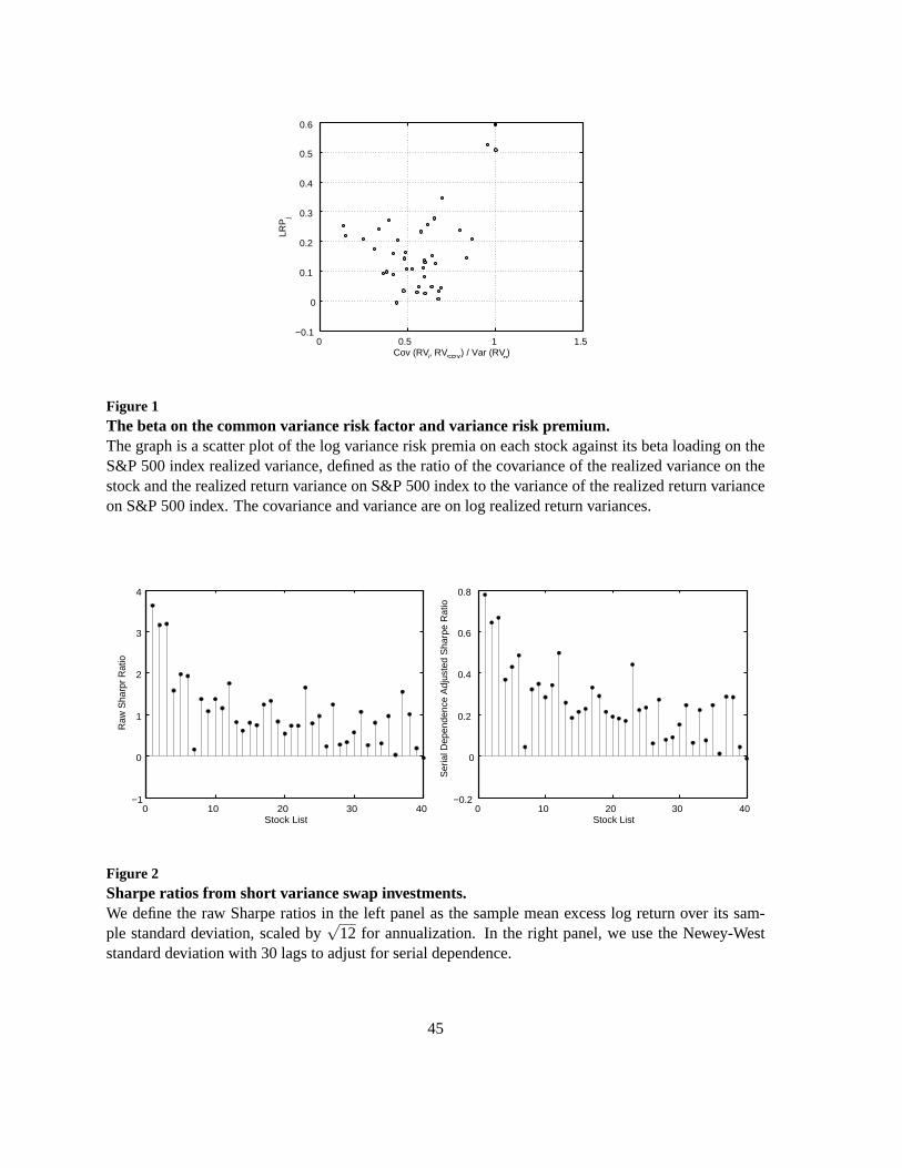
0 0.5 1 1.5−0.1

0

0.1

0.2

0.3

0.4

0.5

0.6

Cov (RVj, RV

SPX) / Var (RV

p)

LRP

j

Figure 1The beta on the common variance risk factor and variance risk premium.The graph is a scatter plot of the log variance risk premia on each stock against its beta loading on theS&P 500 index realized variance, defined as the ratio of the covariance ofthe realized variance on thestock and the realized return variance on S&P 500 index to the variance of the realized return varianceon S&P 500 index. The covariance and variance are on log realized return variances.

0 10 20 30 40−1

0

1

2

3

4

Stock List

Raw

Sha

rpr

Rat

io

0 10 20 30 40−0.2

0

0.2

0.4

0.6

0.8

Stock List

Ser

ial D

epen

denc

e A

djus

ted

Sha

rpe

Rat

io

Figure 2Sharpe ratios from short variance swap investments.We define the raw Sharpe ratios in the left panel as the sample mean excess log return over its sam-ple standard deviation, scaled by

√12 for annualization. In the right panel, we use the Newey-West

standard deviation with 30 lags to adjust for serial dependence.

45

Table 1Model parameters used in the numerical illustration

Model σ λ µj σ j κ σv ρ

BS 0.37MJD 0.35 0.40 −0.09 0.18MJDSV 0.35 0.40 −0.09 0.18 1.04 2.57 −0.70

Market Ft = 100, r = 5.6%.

Under MJDSV,σ =√

θ.

46

Table 2Numerical illustration of the approximation error for variance and volatility swap rates

lnvt/θ Variance Swap Volatility Swap

EQ[RV] SW Error ε[EQ[

√RV]

]2ATMV2 Error

A. Black-Scholes Model

0.0 0.1369 0.1369 0.0000 0.0000 0.1369 0.1369 0.0000

B. Merton Jump-Diffusion Model

0.0 0.1387 0.1366 0.0021 0.0021 0.1318 0.1319 -0.0001

C. MJD-Stochastic Volatility

-3.0 0.0272 0.0265 0.0007 0.0021 0.0111 0.0109 0.0003-2.5 0.0310 0.0310 0.0000 0.0021 0.0149 0.0146 0.0003-2.0 0.0372 0.0380 -0.0007 0.0021 0.0213 0.0212 0.0002-1.5 0.0475 0.0488 -0.0012 0.0021 0.0323 0.0322 0.0001-1.0 0.0645 0.0652 -0.0007 0.0021 0.0504 0.0504 -0.0000-0.5 0.0925 0.0915 0.0010 0.0021 0.0799 0.0799 -0.00000.0 0.1387 0.1363 0.0024 0.0021 0.1279 0.1279 -0.00000.5 0.2148 0.2105 0.0043 0.0021 0.2063 0.2063 0.00001.0 0.3403 0.3344 0.0060 0.0021 0.3347 0.3345 0.00011.5 0.5472 0.5411 0.0061 0.0021 0.5454 0.5451 0.00042.0 0.8884 0.8840 0.0044 0.0021 0.8923 0.8915 0.00082.5 1.4509 1.4510 -0.0001 0.0021 1.4636 1.4618 0.00183.0 2.3782 2.3873 -0.0090 0.0021 2.4056 2.4016 0.0039

Entries under the title “Variance Swap” report the expectedvalue of the annualized variance computed basedon the analytical value (EQ[RV]), the synthetic approximation of the annualized variance swap rate (SW) basedon five European option implied volatility quotes, and the approximation error of this synthetic swap rate (Error= EQ[RV]− SW). The columnε reports the analytical approximation error due to the jump component in theasset price process. Entries under the title “Volatility Swap” reports the square of the expected value of the

realized volatility ([EQ[

√RV]

]2) based on numerical integration, the at-the-money impliedvolatility (ATMV2)

as an approximation, and the approximation error (Error =[EQ[

√RV]

]2−ATMV2). Option prices are computedbased under three option pricing models with model parameters listed in Table 1, assuming an 30-day optionmaturity. For models with stochastic volatility, the first column denotes the log difference between the currentinstantaneous variance levelvt and its long-run meanθ.

47

Table 3List of stocks and stock indexes used in our study

No. Ticker Starting Date Ending Date N NK Name

1 SPX 04-Jan-1996 28-Feb-2003 1779 26 S&P 500 Index2 OEX 04-Jan-1996 28-Feb-2003 1780 27 S&P 100 Index3 DJX 06-Oct-1997 28-Feb-2003 1333 12 Dow Jones Industrial Average4 NDX 04-Jan-1996 28-Feb-2003 1722 19 Nasdaq 100 Stock Index5 QQQ 10-Mar-1999 28-Feb-2003 978 22 Nasdaq-100 Index Tracking Stock

6 MSFT 04-Jan-1996 28-Feb-2003 1766 9 Microsoft Corp7 INTC 04-Jan-1996 28-Feb-2003 1653 8 Intel Corp8 IBM 04-Jan-1996 28-Feb-2003 1768 9 International Business Machines Corp9 AMER 04-Jan-1996 28-Feb-2003 1648 9 Nanobac Pharmaceuticals Inc

10 DELL 04-Jan-1996 28-Feb-2003 1650 7 Dell Inc11 CSCO 04-Jan-1996 28-Feb-2003 1554 7 Cisco Systems Inc12 GE 04-Jan-1996 28-Feb-2003 1458 6 General Electric Co13 CPQ 04-Jan-1996 03-May-2002 1272 6 Compaq Computer Corp14 YHOO 09-Sep-1997 28-Feb-2003 1176 14 Yahoo! Inc15 SUNW 04-Jan-1996 28-Feb-2003 1395 8 Sun Microsystems Inc16 MU 04-Jan-1996 28-Feb-2003 1720 8 Micron Technology Inc17 MO 04-Jan-1996 28-Feb-2003 1474 5 Altria Group Inc18 AMZN 19-Nov-1997 28-Feb-2003 1078 12 Amazon.Com Inc19 ORCL 04-Jan-1996 28-Feb-2003 1104 6 Oracle Corp20 LU 19-Apr-1996 28-Feb-2003 981 7 Lucent Technologies Inc21 TRV 04-Jan-1996 28-Feb-2003 1279 5 Thousand Trails Inc22 WCOM 04-Jan-1996 21-Jun-2002 1104 6 WorldCom Inc23 TYC 05-Jan-1996 28-Feb-2003 979 6 Tyco International Ltd24 AMAT 04-Jan-1996 28-Feb-2003 1671 8 Applied Materials Inc25 QCOM 04-Jan-1996 28-Feb-2003 1613 8 Qualcomm Inc26 TXN 04-Jan-1996 28-Feb-2003 1610 7 Texas Instruments Inc27 PFE 04-Jan-1996 28-Feb-2003 1420 6 Pfizer Inc28 MOT 04-Jan-1996 28-Feb-2003 1223 6 Motorola Inc29 EMC 04-Jan-1996 28-Feb-2003 1188 7 EMC Corp30 HWP 04-Jan-1996 28-Feb-2003 1395 6 Hewlett-Packward Co31 AMGN 04-Jan-1996 28-Feb-2003 1478 6 Amgen Inc32 BRCM 28-Oct-1998 28-Feb-2003 1003 12 Broadcom Corp33 MER 04-Jan-1996 28-Feb-2003 1542 6 Merill Lynch & Co Inc34 NOK 04-Jan-1996 28-Feb-2003 1176 6 Nokia OYJ35 CHL 04-Jan-1996 28-Feb-2003 1422 5 China Mobile Hong KongLtd36 UNPH 16-Sep-1996 28-Feb-2003 745 12 JDS Uniphase Corp37 EBAY 01-Feb-1999 28-Feb-2003 1000 12 eBay Inc38 JNPR 07-Oct-1999 28-Feb-2003 627 15 Juniper Networks Inc39 CIEN 14-May-1997 28-Feb-2003 998 9 Ciena Corp40 BRCD 30-Nov-1999 28-Feb-2003 693 10 Brocade Communications Systems Inc

Entries list the ticker, the starting date, the ending date,the sample length (N), the average number of availablestrikes per maturity (NK), and the full name for each of the five stock indexes and 35 individual stocks used inour study.

48

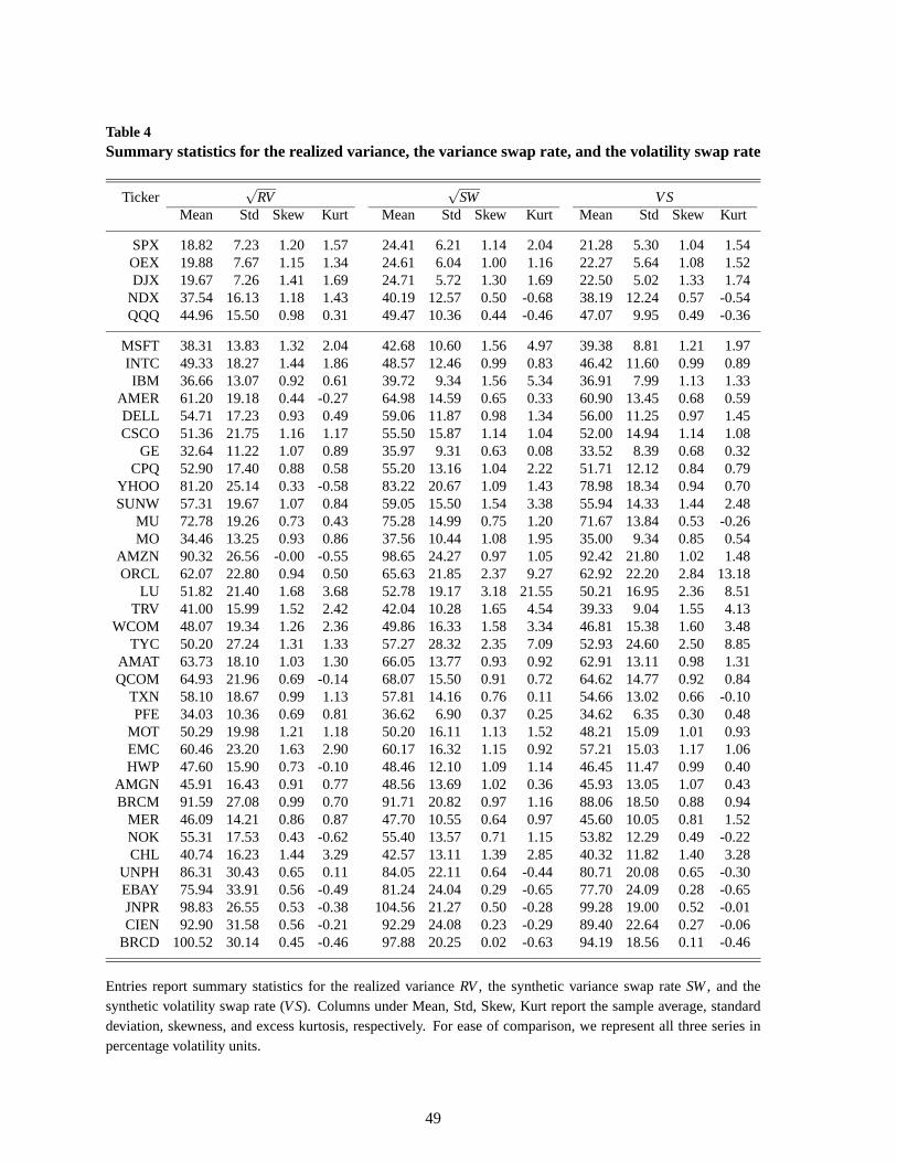
Table 4Summary statistics for the realized variance, the variance swap rate, and the volatility swap rate

Ticker√

RV√

SW VSMean Std Skew Kurt Mean Std Skew Kurt Mean Std Skew Kurt

SPX 18.82 7.23 1.20 1.57 24.41 6.21 1.14 2.04 21.28 5.30 1.04 1.54OEX 19.88 7.67 1.15 1.34 24.61 6.04 1.00 1.16 22.27 5.64 1.08 1.52DJX 19.67 7.26 1.41 1.69 24.71 5.72 1.30 1.69 22.50 5.02 1.33 1.74

NDX 37.54 16.13 1.18 1.43 40.19 12.57 0.50 -0.68 38.19 12.24 0.57 -0.54QQQ 44.96 15.50 0.98 0.31 49.47 10.36 0.44 -0.46 47.07 9.95 0.49 -0.36

MSFT 38.31 13.83 1.32 2.04 42.68 10.60 1.56 4.97 39.38 8.81 1.21 1.97INTC 49.33 18.27 1.44 1.86 48.57 12.46 0.99 0.83 46.42 11.60 0.99 0.89IBM 36.66 13.07 0.92 0.61 39.72 9.34 1.56 5.34 36.91 7.99 1.131.33

AMER 61.20 19.18 0.44 -0.27 64.98 14.59 0.65 0.33 60.90 13.450.68 0.59DELL 54.71 17.23 0.93 0.49 59.06 11.87 0.98 1.34 56.00 11.25 0.97 1.45CSCO 51.36 21.75 1.16 1.17 55.50 15.87 1.14 1.04 52.00 14.94 1.14 1.08

GE 32.64 11.22 1.07 0.89 35.97 9.31 0.63 0.08 33.52 8.39 0.68 0.32CPQ 52.90 17.40 0.88 0.58 55.20 13.16 1.04 2.22 51.71 12.12 0.84 0.79

YHOO 81.20 25.14 0.33 -0.58 83.22 20.67 1.09 1.43 78.98 18.340.94 0.70SUNW 57.31 19.67 1.07 0.84 59.05 15.50 1.54 3.38 55.94 14.33 1.44 2.48

MU 72.78 19.26 0.73 0.43 75.28 14.99 0.75 1.20 71.67 13.84 0.53 -0.26MO 34.46 13.25 0.93 0.86 37.56 10.44 1.08 1.95 35.00 9.34 0.850.54

AMZN 90.32 26.56 -0.00 -0.55 98.65 24.27 0.97 1.05 92.42 21.80 1.02 1.48ORCL 62.07 22.80 0.94 0.50 65.63 21.85 2.37 9.27 62.92 22.20 2.84 13.18

LU 51.82 21.40 1.68 3.68 52.78 19.17 3.18 21.55 50.21 16.95 2.36 8.51TRV 41.00 15.99 1.52 2.42 42.04 10.28 1.65 4.54 39.33 9.04 1.55 4.13

WCOM 48.07 19.34 1.26 2.36 49.86 16.33 1.58 3.34 46.81 15.38 1.60 3.48TYC 50.20 27.24 1.31 1.33 57.27 28.32 2.35 7.09 52.93 24.60 2.50 8.85

AMAT 63.73 18.10 1.03 1.30 66.05 13.77 0.93 0.92 62.91 13.11 0.98 1.31QCOM 64.93 21.96 0.69 -0.14 68.07 15.50 0.91 0.72 64.62 14.770.92 0.84

TXN 58.10 18.67 0.99 1.13 57.81 14.16 0.76 0.11 54.66 13.02 0.66 -0.10PFE 34.03 10.36 0.69 0.81 36.62 6.90 0.37 0.25 34.62 6.35 0.300.48

MOT 50.29 19.98 1.21 1.18 50.20 16.11 1.13 1.52 48.21 15.09 1.01 0.93EMC 60.46 23.20 1.63 2.90 60.17 16.32 1.15 0.92 57.21 15.03 1.17 1.06HWP 47.60 15.90 0.73 -0.10 48.46 12.10 1.09 1.14 46.45 11.47 0.99 0.40

AMGN 45.91 16.43 0.91 0.77 48.56 13.69 1.02 0.36 45.93 13.05 1.07 0.43BRCM 91.59 27.08 0.99 0.70 91.71 20.82 0.97 1.16 88.06 18.50 0.88 0.94

MER 46.09 14.21 0.86 0.87 47.70 10.55 0.64 0.97 45.60 10.05 0.81 1.52NOK 55.31 17.53 0.43 -0.62 55.40 13.57 0.71 1.15 53.82 12.29 0.49 -0.22CHL 40.74 16.23 1.44 3.29 42.57 13.11 1.39 2.85 40.32 11.82 1.40 3.28

UNPH 86.31 30.43 0.65 0.11 84.05 22.11 0.64 -0.44 80.71 20.080.65 -0.30EBAY 75.94 33.91 0.56 -0.49 81.24 24.04 0.29 -0.65 77.70 24.09 0.28 -0.65JNPR 98.83 26.55 0.53 -0.38 104.56 21.27 0.50 -0.28 99.28 19.00 0.52 -0.01CIEN 92.90 31.58 0.56 -0.21 92.29 24.08 0.23 -0.29 89.40 22.64 0.27 -0.06

BRCD 100.52 30.14 0.45 -0.46 97.88 20.25 0.02 -0.63 94.19 18.56 0.11 -0.46

Entries report summary statistics for the realized variance RV, the synthetic variance swap rateSW, and thesynthetic volatility swap rate (VS). Columns under Mean, Std, Skew, Kurt report the sample average, standarddeviation, skewness, and excess kurtosis, respectively. For ease of comparison, we represent all three series inpercentage volatility units.

49

Table 5Summary statistics for variance risk premia

Ticker 100(RV−SW) ln(RV/SW)Mean Std Skew Kurt t Mean Std Skew Kurt t

SPX -2.279 3.339 -0.597 9.283 -7.194 -0.594 0.567 0.220 0.201 -9.484OEX -1.889 3.394 0.633 3.533 -5.458 -0.509 0.560 0.383 -0.041 -7.830DJX -2.039 3.583 0.483 3.622 -5.194 -0.525 0.570 0.660 0.349-7.025

NDX -1.040 10.108 2.043 9.001 -0.944 -0.207 0.455 0.440 0.475 -4.418QQQ -2.940 12.014 1.059 2.840 -1.815 -0.257 0.451 0.176 0.148 -3.887

MSFT -2.746 11.465 -0.446 28.192 -2.850 -0.277 0.496 0.090 0.594 -5.897INTC 2.522 18.632 2.117 6.469 1.356 -0.024 0.500 0.618 0.605-0.523IBM -1.502 10.460 -0.605 19.435 -1.527 -0.232 0.584 -0.009 0.110 -3.901

AMER -3.224 23.125 0.516 1.185 -2.066 -0.173 0.552 -0.094 -0.061 -4.077DELL -3.391 20.005 0.949 3.330 -1.453 -0.208 0.525 0.223 0.095 -3.330CSCO -2.216 19.466 1.549 7.230 -1.321 -0.271 0.813 -6.436 71.559 -3.885

GE -1.893 7.005 1.129 4.758 -3.326 -0.237 0.469 0.339 0.304 -5.487CPQ -1.194 20.799 0.119 5.635 -0.636 -0.136 0.575 0.248 0.213 -2.643

YHOO -1.278 39.162 -0.028 4.412 -0.341 -0.093 0.531 0.123 -0.033 -1.829SUNW -0.570 19.821 -0.641 16.432 -0.310 -0.108 0.465 0.075 0.424 -2.305

MU -2.242 27.831 0.864 4.592 -0.928 -0.097 0.448 0.241 0.462-2.723MO -1.563 11.351 0.883 7.130 -1.388 -0.242 0.676 0.305 0.327-3.661

AMZN -14.587 57.757 -0.137 1.898 -1.668 -0.218 0.569 0.161 -0.066 -2.756ORCL -4.115 44.142 -4.839 34.620 -0.763 -0.151 0.625 -1.8066.914 -2.046

LU -0.105 33.900 -9.996 226.367 -0.047 -0.081 0.518 -0.073 1.199 -1.720TRV 0.632 15.347 2.624 9.165 0.385 -0.127 0.602 0.925 2.028 -1.869

WCOM -0.680 21.542 1.049 11.827 -0.255 -0.130 0.614 -0.067 -0.287 -1.633TYC -8.198 47.826 -1.897 19.373 -1.426 -0.346 0.726 0.907 1.171 -3.996

AMAT -1.627 23.865 1.110 4.803 -0.809 -0.106 0.464 0.259 0.423 -2.624QCOM -1.757 27.014 0.735 1.490 -0.683 -0.158 0.570 -0.193 0.544 -2.700

TXN 1.809 19.425 1.189 4.416 0.961 -0.030 0.456 0.072 0.090 -0.728PFE -1.236 7.661 1.654 5.759 -1.506 -0.205 0.568 -0.152 1.206 -2.949

MOT 1.484 20.113 -0.689 10.783 0.815 -0.044 0.555 -0.477 0.483 -0.796EMC 3.068 27.062 2.241 9.447 0.871 -0.046 0.476 0.357 0.163 -0.915HWP 0.241 14.537 0.465 6.333 0.173 -0.087 0.521 0.214 0.372 -1.656

AMGN -1.679 14.626 0.631 3.782 -1.019 -0.163 0.531 0.078 -0.295 -2.731BRCM 2.783 48.606 0.635 1.918 0.489 -0.035 0.466 0.178 -0.659 -0.602

MER -0.604 12.541 1.021 2.748 -0.497 -0.112 0.485 0.273 -0.070 -2.507NOK 1.131 18.978 -0.593 8.818 0.568 -0.047 0.536 0.056 0.628-0.765CHL -0.606 14.599 2.238 12.212 -0.412 -0.145 0.518 0.298 0.577 -2.674

UNPH 8.221 48.510 0.884 1.940 1.454 -0.006 0.565 -0.328 -0.048 -0.098EBAY -2.613 45.445 1.458 3.265 -0.403 -0.253 0.566 0.422 0.062 -2.614JNPR -9.136 51.393 -0.189 0.783 -1.200 -0.144 0.490 -0.581 0.227 -2.060CIEN 5.299 60.722 0.986 3.740 0.664 -0.032 0.583 0.527 1.491-0.414

BRCD 10.201 56.030 0.747 0.839 1.158 0.007 0.520 -0.219 -0.355 0.089

Entries report summary statistics for variance risk premia, defined as the difference between the realized varianceand the variance swap rate in the columns on the left side and as the log difference in the columns on the rightside. Columns under Mean, Std, Skew, Kurt report the sample average, standard deviation, skewness, and excesskurtosis, respectively. Columns undert report thet-statistics of the mean risk premia. In calculating thet-statistics, we adjust for serial dependence using the Newey-West standard deviation with a lag of 30 days.

50

Table 6Explaining variance risk premia with CAPM beta

Proxy S&P 500 Index Valued-Weighted Market Portfolioα β R2 α β R2

SPX -0.577 ( -12.302 ) -4.589 ( -5.884 ) 0.183 -0.568 ( -9.378 )-5.299 ( -4.623 ) 0.234OEX -0.492 ( -10.293 ) -4.569 ( -5.916 ) 0.186 -0.498 ( -8.007 )-5.335 ( -4.880 ) 0.233DJX -0.532 ( -9.569 ) -4.734 ( -5.407 ) 0.216 -0.531 ( -8.492 ) -4.513 ( -3.761 ) 0.198

NDX -0.198 ( -4.944 ) -2.563 ( -4.065 ) 0.090 -0.151 ( -4.113 ) -3.526 ( -3.242 ) 0.183QQQ -0.267 ( -4.754 ) -1.226 ( -2.015 ) 0.024 -0.238 ( -4.482 ) -2.709 ( -1.568 ) 0.107

MSFT -0.269 ( -6.511 ) -2.255 ( -4.217 ) 0.058 -0.263 ( -4.635 )-2.375 ( -2.844 ) 0.063INTC -0.015 ( -0.325 ) -2.298 ( -2.871 ) 0.059 0.016 ( 0.336 ) -3.669 ( -3.084 ) 0.143IBM -0.223 ( -4.134 ) -2.310 ( -2.876 ) 0.044 -0.183 ( -3.057 ) -2.040 ( -1.665 ) 0.037

AMER -0.162 ( -3.579 ) -2.216 ( -3.269 ) 0.043 -0.167 ( -3.530 )-1.521 ( -1.459 ) 0.022DELL -0.196 ( -3.881 ) -2.678 ( -3.613 ) 0.073 -0.189 ( -2.715 )-3.224 ( -3.408 ) 0.110CSCO -0.266 ( -3.577 ) -0.957 ( -0.599 ) 0.004 -0.217 ( -3.195 )-1.927 ( -0.855 ) 0.040

GE -0.230 ( -5.731 ) -2.593 ( -3.798 ) 0.092 -0.227 ( -4.284 ) -1.621 ( -1.512 ) 0.046CPQ -0.110 ( -1.975 ) -2.398 ( -2.312 ) 0.039 0.047 ( 0.909 ) -3.318 ( -2.762 ) 0.101

YHOO -0.094 ( -1.702 ) -0.593 ( -0.813 ) 0.004 -0.109 ( -1.745 )0.831 ( 0.776 ) 0.008SUNW -0.089 ( -2.080 ) -2.380 ( -3.371 ) 0.062 -0.049 ( -0.899 )-3.951 ( -3.187 ) 0.179

MU -0.092 ( -2.498 ) -1.350 ( -2.234 ) 0.025 -0.049 ( -1.095 ) -2.512 ( -3.606 ) 0.094MO -0.244 ( -3.906 ) 0.482 ( 0.540 ) 0.001 -0.180 ( -2.942 ) 0.702 ( 0.604 ) 0.003

AMZN -0.218 ( -3.289 ) 0.120 ( 0.122 ) 0.000 -0.054 ( -0.671 ) 0.284 ( 0.306 ) 0.001ORCL -0.141 ( -2.041 ) -2.206 ( -2.597 ) 0.032 -0.124 ( -1.697 )-3.674 ( -2.567 ) 0.116

LU -0.068 ( -1.376 ) -1.436 ( -1.732 ) 0.019 0.030 ( 0.634 ) -2.736 ( -2.849 ) 0.103TRV -0.126 ( -2.047 ) -1.993 ( -2.567 ) 0.035 -0.097 ( -0.980 ) -1.022 ( -0.647 ) 0.011

WCOM -0.101 ( -1.405 ) -3.430 ( -3.307 ) 0.075 -0.006 ( -0.068 ) -4.137 ( -2.691 ) 0.129TYC -0.353 ( -4.066 ) -1.724 ( -1.490 ) 0.018 -0.321 ( -3.137 ) 0.923 ( 0.308 ) 0.003

AMAT -0.102 ( -2.598 ) -1.080 ( -1.968 ) 0.015 -0.054 ( -1.175 )-2.736 ( -3.498 ) 0.104QCOM -0.154 ( -2.889 ) -1.305 ( -1.646 ) 0.015 -0.089 ( -1.578 )-2.578 ( -2.202 ) 0.062

TXN -0.028 ( -0.677 ) -0.724 ( -1.346 ) 0.007 -0.032 ( -0.621 ) -0.714 ( -0.887 ) 0.007PFE -0.200 ( -3.342 ) -1.957 ( -1.878 ) 0.036 -0.149 ( -2.455 ) -1.909 ( -1.246 ) 0.037

MOT -0.031 ( -0.581 ) -1.954 ( -1.861 ) 0.031 0.032 ( 0.441 ) -3.523 ( -2.044 ) 0.106EMC -0.031 ( -0.682 ) -2.611 ( -3.398 ) 0.081 -0.028 ( -0.389 ) -3.146 ( -3.890 ) 0.131HWP -0.076 ( -1.530 ) -1.661 ( -1.956 ) 0.025 0.010 ( 0.185 ) -1.956 ( -1.536 ) 0.049

AMGN -0.162 ( -3.050 ) -1.129 ( -1.281 ) 0.014 -0.045 ( -0.556 )-0.127 ( -0.091 ) 0.000BRCM -0.029 ( -0.533 ) 0.878 ( 1.172 ) 0.011 -0.013 ( -0.146 ) -0.613 ( -0.304 ) 0.004

MER -0.109 ( -2.493 ) -1.363 ( -1.739 ) 0.024 -0.081 ( -1.333 ) -1.271 ( -1.162 ) 0.022NOK -0.046 ( -0.792 ) -1.715 ( -1.933 ) 0.030 0.028 ( 0.442 ) -1.928 ( -1.490 ) 0.059CHL -0.140 ( -2.692 ) -1.609 ( -1.805 ) 0.029 -0.053 ( -1.269 ) -1.953 ( -2.115 ) 0.052

UNPH -0.005 ( -0.085 ) -1.444 ( -1.258 ) 0.018 0.011 ( 0.297 ) -2.982 ( -1.201 ) 0.073EBAY -0.252 ( -3.216 ) 0.173 ( 0.171 ) 0.000 -0.206 ( -1.633 ) 0.018 ( 0.014 ) 0.000JNPR -0.147 ( -2.154 ) -0.490 ( -0.575 ) 0.003 -0.133 ( -1.720 )-1.912 ( -0.924 ) 0.034CIEN -0.027 ( -0.361 ) -2.422 ( -1.827 ) 0.046 -0.011 ( -0.122 )-4.399 ( -1.924 ) 0.154

BRCD 0.008 ( 0.110 ) 0.104 ( 0.111 ) 0.000 0.078 ( 0.811 ) -2.497( -1.941 ) 0.086

Entries report the GMM estimates (andt-statistics in parentheses) of the following relation,

lnRVt,T/SWt,T = α+β j ERmt,T +e,

whereERm denotes the excess return on the market portfolio, which is proxyed by the return on the S&P 500index forward in the left panel and the excess return on the CRSP valued-weighted stock portfolio in the rightpanel. Thet-statistics are computed according to Newey and West (1987)with 30 lags for the overlapping dailyseries in the left panel and six lags for the non-overlappingmonthly series in the right panel. The columns under“R2” report the unadjusted R-squared of the regression.

51

Table 7Explaining variance risk premia with Fama-French risk factors

Ticker α ERm SMB HML R2

SPX -0.561 ( -8.365 ) -5.038 ( -3.765 ) -2.831 ( -2.132 ) -0.287( -0.342 ) 0.276OEX -0.489 ( -7.311 ) -5.090 ( -3.992 ) -3.344 ( -2.483 ) -0.509( -0.570 ) 0.289DJX -0.518 ( -7.447 ) -4.434 ( -3.201 ) -3.637 ( -3.150 ) -1.327( -1.692 ) 0.273

NDX -0.150 ( -4.032 ) -2.777 ( -2.635 ) -1.948 ( -2.472 ) 1.351 (1.836 ) 0.272QQQ -0.221 ( -4.184 ) -1.932 ( -1.309 ) -1.851 ( -1.784 ) 1.504 (2.651 ) 0.235

MSFT -0.247 ( -5.054 ) -2.469 ( -2.865 ) -4.939 ( -5.170 ) -1.976 ( -2.289 ) 0.222INTC 0.023 ( 0.567 ) -3.770 ( -3.207 ) -2.823 ( -2.746 ) -1.156 (-1.519 ) 0.194IBM -0.174 ( -3.371 ) -1.934 ( -1.535 ) -3.053 ( -1.931 ) -0.782( -0.510 ) 0.085

AMER -0.153 ( -3.765 ) -1.576 ( -1.173 ) -3.291 ( -2.377 ) -1.125 ( -1.124 ) 0.084DELL -0.187 ( -2.733 ) -2.673 ( -3.190 ) -3.118 ( -2.544 ) 0.401( 0.338 ) 0.190CSCO -0.227 ( -3.598 ) -1.009 ( -0.444 ) 1.288 ( 1.026 ) 2.082 ( 2.389 ) 0.076

GE -0.208 ( -4.997 ) -1.512 ( -1.294 ) -2.617 ( -2.689 ) -0.738 (-0.884 ) 0.121CPQ 0.046 ( 0.959 ) -3.024 ( -2.112 ) 1.069 ( 0.927 ) 0.847 ( 0.809 ) 0.108

YHOO -0.107 ( -1.738 ) 0.144 ( 0.109 ) 0.574 ( 0.363 ) -0.975 ( -0.894 ) 0.029SUNW -0.056 ( -1.079 ) -3.113 ( -2.087 ) -1.509 ( -1.472 ) 0.997( 0.959 ) 0.224

MU -0.046 ( -1.072 ) -2.704 ( -3.663 ) -0.346 ( -0.403 ) -0.617 (-0.950 ) 0.099MO -0.187 ( -3.145 ) 0.939 ( 0.688 ) -0.306 ( -0.169 ) 0.883 ( 0.622 ) 0.008

AMZN -0.063 ( -0.911 ) -0.367 ( -0.259 ) -1.682 ( -0.726 ) -1.887 ( -1.180 ) 0.043ORCL -0.119 ( -1.570 ) -3.893 ( -3.237 ) -0.264 ( -0.172 ) -0.377 ( -0.413 ) 0.117

LU 0.031 ( 0.652 ) -3.475 ( -2.738 ) -0.859 ( -0.544 ) -1.438 ( -1.364 ) 0.133TRV -0.059 ( -0.763 ) -0.463 ( -0.277 ) -5.841 ( -5.029 ) -1.069( -1.016 ) 0.218

WCOM -0.014 ( -0.157 ) -4.793 ( -2.656 ) -2.345 ( -1.403 ) -1.784( -1.558 ) 0.157TYC -0.282 ( -2.585 ) 0.404 ( 0.173 ) -4.381 ( -1.565 ) -2.715 ( -1.850 ) 0.087

AMAT -0.036 ( -1.064 ) -2.508 ( -2.905 ) -4.070 ( -4.315 ) -1.068 ( -1.780 ) 0.247QCOM -0.090 ( -1.600 ) -1.744 ( -1.446 ) -3.711 ( -3.344 ) 0.604( 0.581 ) 0.135

TXN -0.020 ( -0.400 ) -0.949 ( -1.439 ) -4.230 ( -4.987 ) -1.954( -2.125 ) 0.155PFE -0.129 ( -2.541 ) -1.528 ( -0.865 ) -3.535 ( -1.956 ) -1.073( -0.551 ) 0.103

MOT 0.028 ( 0.353 ) -3.038 ( -1.893 ) 0.784 ( 0.541 ) 0.817 ( 0.737 ) 0.114EMC -0.030 ( -0.491 ) -1.651 ( -1.707 ) -1.965 ( -2.401 ) 1.761 (2.539 ) 0.259HWP 0.014 ( 0.250 ) -2.384 ( -1.600 ) -0.826 ( -0.690 ) -1.046 ( -0.946 ) 0.061

AMGN -0.040 ( -0.550 ) -0.426 ( -0.287 ) -1.142 ( -0.844 ) -1.194 ( -1.485 ) 0.018BRCM 0.023 ( 0.290 ) -0.094 ( -0.042 ) -3.281 ( -2.507 ) -0.535 (-0.444 ) 0.086

MER -0.075 ( -1.393 ) -0.899 ( -0.762 ) -1.881 ( -1.324 ) 0.297 (0.332 ) 0.060NOK 0.043 ( 0.651 ) -1.874 ( -1.517 ) -2.407 ( -2.105 ) -0.815 ( -0.947 ) 0.115CHL -0.050 ( -1.300 ) -1.816 ( -1.952 ) -2.762 ( -2.195 ) -0.531( -0.593 ) 0.111

UNPH 0.028 ( 0.418 ) -1.791 ( -0.796 ) -1.815 ( -1.015 ) 1.128 ( 0.798 ) 0.148EBAY -0.177 ( -1.373 ) 0.590 ( 0.536 ) -2.783 ( -1.993 ) 0.300 ( 0.268 ) 0.072JNPR -0.049 ( -0.686 ) -3.209 ( -2.277 ) -3.556 ( -2.444 ) -3.600 ( -3.620 ) 0.173CIEN 0.011 ( 0.119 ) -5.258 ( -2.452 ) -2.997 ( -2.526 ) -2.506 (-1.584 ) 0.211

BRCD 0.138 ( 1.155 ) -1.766 ( -1.485 ) -3.769 ( -2.599 ) -0.966 (-0.782 ) 0.225

Entries report the GMM estimates (andt-statistics in parentheses) of the following relation,

lnRVt,T/SWt,T = α+βERmt,T +sSMBt,T +hHMLt,T +e,

where the regressors are the three stock-market risk factors defined by Fama and French (1993): the excessreturn on the market portfolio (ERm), the size factor (SMB), and the book-to-market factor (HML). The dataare monthly from January 1996 to December 2002. Thet-statistics are computed according to Newey and West(1987) with six lags. The columns under “R2” report the unadjusted R-squared of the regression.

52

Table 8Expectation hypothesis regressions on constant variance risk premia

Ticker RVt,T = a+bSWt,T +e lnRVt,T = a+blnSWt,T +ea b R2 a b R2

SPX 0.729 ( 1.148 ) 0.526 ( -3.981 ) 0.293 -0.492 ( -2.385 ) 0.941 ( -0.505 ) 0.391OEX 0.466 ( 0.740 ) 0.633 ( -3.137 ) 0.315 -0.531 ( -2.534 ) 1.012 ( 0.104 ) 0.418DJX 1.007 ( 1.243 ) 0.527 ( -3.361 ) 0.223 -0.183 ( -0.696 ) 0.806 ( -1.319 ) 0.269

NDX -2.547 ( -1.508 ) 1.085 ( 0.648 ) 0.585 -0.421 ( -2.272 ) 1.080 ( 1.158 ) 0.690QQQ -4.281 ( -1.435 ) 1.052 ( 0.364 ) 0.473 -0.655 ( -1.778 ) 1.126 ( 1.070 ) 0.523

MSFT 3.042 ( 1.358 ) 0.701 ( -2.209 ) 0.333 -0.254 ( -0.968 ) 0.992 ( -0.087 ) 0.453INTC 2.351 ( 0.656 ) 1.007 ( 0.039 ) 0.358 0.325 ( 1.236 ) 0.888 (-1.276 ) 0.430IBM 4.737 ( 1.885 ) 0.625 ( -2.239 ) 0.244 0.143 ( 0.502 ) 0.862 (-1.320 ) 0.290

AMER 12.920 ( 3.494 ) 0.636 ( -4.607 ) 0.263 0.562 ( 1.439 ) 0.801 ( -1.969 ) 0.296DELL 8.643 ( 2.092 ) 0.668 ( -2.565 ) 0.224 0.507 ( 1.192 ) 0.797( -1.666 ) 0.257CSCO -2.402 ( -0.871 ) 1.006 ( 0.055 ) 0.534 -0.811 ( -1.705 ) 1.161 ( 1.239 ) 0.367

GE 1.309 ( 1.240 ) 0.768 ( -2.661 ) 0.407 0.047 ( 0.272 ) 0.886 ( -1.612 ) 0.488CPQ 13.279 ( 3.027 ) 0.551 ( -2.977 ) 0.182 0.846 ( 1.742 ) 0.708( -2.083 ) 0.251

YHOO 27.022 ( 3.714 ) 0.615 ( -4.217 ) 0.313 0.696 ( 1.538 ) 0.811 ( -1.860 ) 0.344SUNW 5.287 ( 1.163 ) 0.843 ( -1.105 ) 0.483 0.089 ( 0.245 ) 0.944( -0.555 ) 0.481

MU 17.606 ( 3.873 ) 0.663 ( -4.220 ) 0.273 0.971 ( 2.806 ) 0.733 (-3.121 ) 0.299MO 6.654 ( 4.740 ) 0.459 ( -6.258 ) 0.146 0.539 ( 1.978 ) 0.697 ( -2.956 ) 0.238

AMZN 53.943 ( 4.739 ) 0.336 ( -7.649 ) 0.140 1.013 ( 1.421 ) 0.728 ( -1.819 ) 0.276ORCL 30.942 ( 3.241 ) 0.267 ( -3.026 ) 0.108 1.046 ( 1.254 ) 0.674 ( -1.366 ) 0.288

LU 18.249 ( 2.730 ) 0.418 ( -2.631 ) 0.220 0.338 ( 1.216 ) 0.870 (-1.505 ) 0.492TRV 4.393 ( 1.623 ) 0.799 ( -1.694 ) 0.237 0.414 ( 1.171 ) 0.808 (-1.578 ) 0.266

WCOM 9.398 ( 3.237 ) 0.634 ( -2.599 ) 0.304 0.472 ( 1.308 ) 0.807 (-1.681 ) 0.377TYC 18.120 ( 3.902 ) 0.355 ( -18.024 ) 0.246 0.059 ( 0.208 ) 0.878 ( -1.629 ) 0.480

AMAT 12.450 ( 3.235 ) 0.691 ( -3.314 ) 0.267 0.837 ( 2.634 ) 0.748 ( -2.962 ) 0.302QCOM 8.678 ( 1.893 ) 0.786 ( -2.259 ) 0.327 0.469 ( 1.130 ) 0.835( -1.539 ) 0.292

TXN 4.316 ( 1.069 ) 0.929 ( -0.506 ) 0.429 0.332 ( 1.113 ) 0.895 (-1.214 ) 0.466PFE 4.546 ( 2.892 ) 0.584 ( -4.106 ) 0.150 0.501 ( 1.664 ) 0.724 (-2.552 ) 0.195

MOT 6.500 ( 1.977 ) 0.820 ( -1.157 ) 0.394 0.498 ( 1.725 ) 0.827 (-1.773 ) 0.449EMC -2.871 ( -0.559 ) 1.153 ( 0.852 ) 0.493 0.116 ( 0.334 ) 0.954( -0.454 ) 0.502HWP 6.807 ( 2.461 ) 0.737 ( -2.375 ) 0.332 0.340 ( 1.193 ) 0.862 ( -1.549 ) 0.377

AMGN 5.241 ( 2.190 ) 0.728 ( -2.354 ) 0.389 0.196 ( 0.700 ) 0.884( -1.330 ) 0.437BRCM 23.907 ( 1.813 ) 0.761 ( -1.396 ) 0.320 1.045 ( 2.194 ) 0.754 ( -2.249 ) 0.343

MER 4.187 ( 1.369 ) 0.799 ( -1.399 ) 0.333 0.376 ( 1.188 ) 0.841 (-1.563 ) 0.373NOK 12.659 ( 2.964 ) 0.646 ( -2.579 ) 0.261 0.699 ( 1.776 ) 0.778( -1.995 ) 0.338CHL 4.234 ( 2.136 ) 0.756 ( -1.912 ) 0.352 0.005 ( 0.021 ) 0.946 (-0.632 ) 0.518

UNPH 18.161 ( 1.653 ) 0.868 ( -0.696 ) 0.349 0.514 ( 1.014 ) 0.876 ( -1.014 ) 0.389EBAY 2.708 ( 0.282 ) 0.926 ( -0.516 ) 0.415 -1.256 ( -3.506 ) 1.245 ( 2.857 ) 0.663JNPR 32.793 ( 2.113 ) 0.632 ( -2.301 ) 0.274 1.506 ( 2.419 ) 0.646 ( -2.553 ) 0.235CIEN 38.400 ( 2.601 ) 0.636 ( -2.280 ) 0.204 1.113 ( 1.848 ) 0.738 ( -1.971 ) 0.337

BRCD 24.059 ( 1.628 ) 0.861 ( -0.846 ) 0.277 1.026 ( 1.622 ) 0.774 ( -1.615 ) 0.299

Entries report the GMM estimates (andt-statistics in parentheses) of the following relations,

Left panel: RVt,T = a+bSWt,T +e,Right panel: lnRVt,T = a+b lnSWt,T +e.

The t-statistics are calculated according to Newey and West (1987) with 30 lags, under the null hypothesis ofa = 0,b = 1. The columns under “R2” report the unadjusted R-squared of the regression.

53

Table 9Variance risk premia and variance of return volatility

Ticker lnSWt,T/RVt,T = a+b(SWt,T −VS2

t

)+e lnSWt,T/RVt,T = a+bln

(SWt,T/VS2

t

)+e

a b R2 a b R2

SPX 0.462 ( 7.001 ) 0.087 ( 3.117 ) 0.048 0.283 ( 4.052 ) 1.142 ( 6.233 ) 0.086OEX 0.412 ( 4.598 ) 0.085 ( 1.355 ) 0.013 0.295 ( 3.218 ) 1.055 ( 2.929 ) 0.028DJX 0.379 ( 4.258 ) 0.130 ( 2.386 ) 0.049 0.302 ( 3.007 ) 1.211 ( 3.241 ) 0.048

NDX 0.204 ( 4.049 ) 0.002 ( 0.092 ) 0.000 0.154 ( 2.701 ) 0.505 ( 1.306 ) 0.006QQQ 0.232 ( 3.641 ) 0.010 ( 0.859 ) 0.003 0.189 ( 2.563 ) 0.671 ( 1.621 ) 0.011

MSFT 0.234 ( 5.065 ) 0.014 ( 3.037 ) 0.023 0.194 ( 3.255 ) 0.547 (2.137 ) 0.019INTC -0.012 ( -0.189 ) 0.016 ( 0.715 ) 0.004 -0.002 ( -0.032 ) 0.299 ( 0.444 ) 0.001IBM 0.168 ( 2.839 ) 0.027 ( 4.342 ) 0.035 0.049 ( 0.723 ) 1.294 ( 4.945 ) 0.050

AMER 0.107 ( 1.834 ) 0.012 ( 2.397 ) 0.015 0.114 ( 1.975 ) 0.455 (1.639 ) 0.007DELL 0.106 ( 1.690 ) 0.028 ( 2.527 ) 0.028 0.087 ( 1.182 ) 1.137 (2.150 ) 0.022CSCO 0.293 ( 3.376 ) -0.005 ( -0.530 ) 0.001 0.210 ( 3.000 ) 0.469 ( 1.172 ) 0.003

GE 0.156 ( 3.410 ) 0.043 ( 2.877 ) 0.039 0.126 ( 2.725 ) 0.813 ( 4.186 ) 0.045CPQ 0.055 ( 0.965 ) 0.020 ( 5.554 ) 0.071 0.004 ( 0.070 ) 1.017 ( 6.947 ) 0.059

YHOO 0.052 ( 0.858 ) 0.005 ( 4.437 ) 0.021 0.040 ( 0.652 ) 0.545 (2.071 ) 0.013SUNW 0.062 ( 1.300 ) 0.012 ( 6.099 ) 0.038 0.035 ( 0.669 ) 0.685 (3.308 ) 0.029

MU 0.050 ( 1.340 ) 0.008 ( 3.342 ) 0.026 0.044 ( 1.161 ) 0.548 ( 2.760 ) 0.016MO 0.165 ( 2.547 ) 0.037 ( 2.381 ) 0.050 0.133 ( 2.058 ) 0.792 ( 2.414 ) 0.040

AMZN 0.047 ( 0.535 ) 0.013 ( 4.195 ) 0.084 0.023 ( 0.264 ) 1.545 (4.041 ) 0.050ORCL 0.300 ( 3.285 ) -0.045 ( -2.982 ) 0.175 0.310 ( 1.790 ) -1.761 ( -1.335 ) 0.036

LU 0.053 ( 1.034 ) 0.008 ( 9.332 ) 0.053 0.045 ( 0.744 ) 0.396 ( 1.720 ) 0.009TRV 0.060 ( 0.796 ) 0.027 ( 1.617 ) 0.015 -0.046 ( -0.531 ) 1.347( 2.944 ) 0.040

WCOM -0.017 ( -0.210 ) 0.045 ( 5.860 ) 0.108 -0.046 ( -0.569 ) 1.396 ( 7.922 ) 0.095TYC 0.270 ( 2.818 ) 0.011 ( 4.095 ) 0.039 0.245 ( 2.472 ) 0.734 ( 1.700 ) 0.012

AMAT 0.003 ( 0.072 ) 0.024 ( 3.123 ) 0.047 0.014 ( 0.272 ) 0.944 (2.550 ) 0.026QCOM 0.098 ( 1.461 ) 0.012 ( 1.470 ) 0.010 0.097 ( 1.284 ) 0.588 (1.118 ) 0.005

TXN -0.047 ( -0.987 ) 0.020 ( 3.337 ) 0.040 -0.083 ( -1.552 ) 1.027 ( 4.236 ) 0.040PFE 0.109 ( 1.799 ) 0.064 ( 4.318 ) 0.047 0.068 ( 1.245 ) 1.231 ( 3.997 ) 0.059

MOT 0.004 ( 0.069 ) 0.018 ( 3.217 ) 0.040 -0.053 ( -0.940 ) 1.245( 7.698 ) 0.058EMC 0.033 ( 0.684 ) 0.003 ( 0.613 ) 0.002 0.017 ( 0.342 ) 0.299 ( 1.352 ) 0.006HWP 0.046 ( 0.890 ) 0.020 ( 4.596 ) 0.022 0.036 ( 0.661 ) 0.605 ( 2.273 ) 0.011

AMGN 0.084 ( 1.490 ) 0.030 ( 2.701 ) 0.032 0.030 ( 0.535 ) 1.187 (3.188 ) 0.036BRCM -0.039 ( -0.674 ) 0.010 ( 2.475 ) 0.039 -0.079 ( -1.342 ) 1.521 ( 3.027 ) 0.049

MER -0.026 ( -0.422 ) 0.067 ( 3.737 ) 0.070 -0.025 ( -0.393 ) 1.547 ( 3.603 ) 0.053NOK 0.019 ( 0.306 ) 0.014 ( 4.730 ) 0.031 0.012 ( 0.184 ) 0.692 ( 2.930 ) 0.023CHL 0.079 ( 1.335 ) 0.031 ( 4.601 ) 0.042 0.038 ( 0.607 ) 1.061 ( 5.001 ) 0.042

UNPH -0.024 ( -0.355 ) 0.005 ( 0.850 ) 0.004 0.006 ( 0.101 ) -0.008 ( -0.016 ) 0.000EBAY 0.156 ( 1.494 ) 0.017 ( 1.554 ) 0.020 -0.143 ( -1.336 ) 4.018 ( 5.897 ) 0.217JNPR 0.067 ( 0.696 ) 0.007 ( 1.104 ) 0.022 0.118 ( 1.056 ) 0.260 (0.285 ) 0.001CIEN -0.044 ( -0.522 ) 0.013 ( 2.144 ) 0.027 0.032 ( 0.388 ) 0.005 ( 0.005 ) 0.000

BRCD -0.075 ( -0.762 ) 0.009 ( 1.095 ) 0.018 -0.055 ( -0.547 ) 0.668 ( 0.766 ) 0.007

Entries report the estimates (andt-statistics in parentheses) of the following two regressions in the left and rightpanels, respectively,

lnSWt,T/RVt,T = a+b(SWt,T −VS2

t

)+e,

lnSWt,T/RVt,T = a+b ln(SWt,T/VS2

t

)+e.

The t-statistics are calculated according to Newey and West (1987) with 30 lags, under the null hypothesis ofa = 0,b = 0. The columns under “R2” report the unadjusted R-squared of the regression.

54

Table 10Expectation hypothesis regression on variance risk premia controlling for variance of volatility

Ticker a b c R2

SPX -0.293 ( -1.517 ) 1.007 ( 0.058 ) -1.146 ( -6.090 ) 0.442OEX -0.296 ( -1.328 ) 1.001 ( 0.005 ) -1.055 ( -2.935 ) 0.434DJX -0.113 ( -0.436 ) 0.878 ( -0.874 ) -1.072 ( -3.106 ) 0.295

NDX -0.363 ( -1.833 ) 1.076 ( 1.106 ) -0.459 ( -1.188 ) 0.692QQQ -0.602 ( -1.672 ) 1.132 ( 1.120 ) -0.708 ( -1.674 ) 0.529

MSFT -0.371 ( -1.431 ) 1.068 ( 0.704 ) -0.651 ( -2.424 ) 0.465INTC 0.325 ( 1.241 ) 0.886 ( -1.319 ) 0.047 ( 0.074 ) 0.430IBM 0.033 ( 0.125 ) 0.967 ( -0.331 ) -1.243 ( -4.732 ) 0.319

AMER 0.554 ( 1.412 ) 0.814 ( -1.786 ) -0.308 ( -1.017 ) 0.298DELL 0.569 ( 1.406 ) 0.811 ( -1.588 ) -1.056 ( -1.974 ) 0.271CSCO -0.760 ( -1.642 ) 1.166 ( 1.271 ) -0.527 ( -1.277 ) 0.369

GE 0.031 ( 0.180 ) 0.933 ( -0.960 ) -0.739 ( -3.990 ) 0.506CPQ 0.805 ( 1.721 ) 0.754 ( -1.782 ) -0.874 ( -4.576 ) 0.285

YHOO 0.626 ( 1.277 ) 0.835 ( -1.431 ) -0.307 ( -0.819 ) 0.346SUNW 0.048 ( 0.134 ) 0.976 ( -0.239 ) -0.666 ( -2.950 ) 0.494

MU 0.929 ( 2.602 ) 0.752 ( -2.756 ) -0.355 ( -1.657 ) 0.303MO 0.509 ( 1.891 ) 0.741 ( -2.538 ) -0.612 ( -1.928 ) 0.256

AMZN 0.861 ( 1.198 ) 0.794 ( -1.312 ) -1.165 ( -2.717 ) 0.295ORCL 0.833 ( 1.216 ) 0.698 ( -1.434 ) 1.402 ( 1.640 ) 0.305

LU 0.311 ( 1.149 ) 0.885 ( -1.331 ) -0.244 ( -1.002 ) 0.493TRV 0.341 ( 1.021 ) 0.887 ( -1.010 ) -1.160 ( -2.914 ) 0.285

WCOM 0.530 ( 1.524 ) 0.842 ( -1.402 ) -1.319 ( -6.742 ) 0.431TYC 0.028 ( 0.098 ) 0.904 ( -1.248 ) -0.409 ( -0.968 ) 0.481

AMAT 0.851 ( 2.782 ) 0.765 ( -2.854 ) -0.814 ( -2.259 ) 0.316QCOM 0.507 ( 1.213 ) 0.839 ( -1.496 ) -0.535 ( -0.996 ) 0.296

TXN 0.318 ( 1.079 ) 0.930 ( -0.819 ) -0.955 ( -4.014 ) 0.484PFE 0.448 ( 1.487 ) 0.792 ( -1.804 ) -1.083 ( -3.143 ) 0.232

MOT 0.482 ( 1.718 ) 0.860 ( -1.427 ) -1.118 ( -5.689 ) 0.475EMC 0.084 ( 0.244 ) 0.970 ( -0.293 ) -0.269 ( -1.300 ) 0.505HWP 0.344 ( 1.219 ) 0.875 ( -1.418 ) -0.524 ( -2.093 ) 0.382

AMGN 0.285 ( 1.016 ) 0.897 ( -1.190 ) -1.143 ( -3.162 ) 0.455BRCM 0.784 ( 1.547 ) 0.830 ( -1.429 ) -0.975 ( -1.996 ) 0.353

MER 0.361 ( 1.189 ) 0.887 ( -1.166 ) -1.412 ( -3.219 ) 0.400NOK 0.598 ( 1.433 ) 0.815 ( -1.541 ) -0.423 ( -1.487 ) 0.343CHL -0.066 ( -0.283 ) 1.011 ( 0.126 ) -1.081 ( -4.402 ) 0.536

UNPH 0.600 ( 1.131 ) 0.847 ( -1.167 ) 0.460 ( 0.806 ) 0.391EBAY -0.133 ( -0.308 ) 1.061 ( 0.646 ) -3.755 ( -5.153 ) 0.717JNPR 1.664 ( 2.546 ) 0.598 ( -2.653 ) 0.648 ( 0.702 ) 0.241CIEN 1.232 ( 2.063 ) 0.697 ( -2.246 ) 1.073 ( 1.100 ) 0.344

BRCD 1.015 ( 1.642 ) 0.778 ( -1.591 ) -0.050 ( -0.055 ) 0.299

Entries report the GMM estimates (andt-statistics in parentheses) of the following relation,

lnRVt,T = a+blnSWt,T +cln(SWt,T/VS2

t

)+e.

The t-statistics are calculated according to Newey and West (1987) with 30 lags, under the null hypothesis ofa = 0,b = 1,c = 0. The columns under “R2” report the unadjusted R-squared of the regression.

55