Finance and Economics Discussion SeriesDivisions of Research & Statistics and Monetary Affairs

Federal Reserve Board, Washington, D.C.

Credit Default Swap Spreads and Variance Risk Premia

Hao Wang, Hao Zhou, and Yi Zhou

2011-02

NOTE: Staff working papers in the Finance and Economics Discussion Series (FEDS) are preliminarymaterials circulated to stimulate discussion and critical comment. The analysis and conclusions set forthare those of the authors and do not indicate concurrence by other members of the research staff or theBoard of Governors. References in publications to the Finance and Economics Discussion Series (other thanacknowledgement) should be cleared with the author(s) to protect the tentative character of these papers.

Credit Default Swap Spreads and Variance Risk Premia∗

Hao Wang† Hao Zhou‡ Yi Zhou§

First Draft: August 2009This Version: October 2010

Abstract

We find that firm-level variance risk premium, estimated as the difference between

option-implied and expected variances, has a prominent explanatory power for credit

spreads in the presence of market- and firm-level risk control variables identified in

the existing literature. Such a predictability complements that of the leading state

variable—leverage ratio—and strengthens significantly with lower firm credit rating,

longer credit contract maturity, and model-free implied variance. We provide further

evidence that: (1) variance risk premium has a cleaner systematic component and

Granger-causes implied and expected variances, (2) the cross-section of firms’ variance

risk premia seem to price the market variance risk correctly, and (3) a structural

model with stochastic volatility can reproduce the predictability pattern of variance

risk premia for credit spreads.

JEL Classification: G12, G13, G14.

Keywords: Variance Risk Premia, Credit Default Swap Spreads, Option-implied Vari-

ance, Expected Variance, Realized Variance.

∗We would like to thank Turan Bali, Michael Brennan, Darrell Duffie, Louis Ederington, Robert Geske,Bing Han, Jean Helwege, Robert Jarrow, George Jiang, William Megginson, George Tauchen, Marliese Uhrig-Homburg, Jan Werner, Yelena Larkin, Liuren Wu, Yuhang Xing, Hong Yan; seminar participants at TsinghuaUniversity, University of Oklahoma, University of Texas at Dallas, University of South Carolina, BaruchCollege; and conference participants at FDIC, FIRS, CICF, EFA, and FMA for helpful discussions. Theauthors acknowledge the generous financial support from Global Association of Risk Professionals (GARP)and Center for Hedge Fund Research (CHFR) at Imperial College London.†Tsinghua University, School of Economics and Management, 318 Weilun Building, Beijing 100084, China,

E-mail: wanghao@sem.tsinghua.edu.cn, Tel: 86 10-62797482.‡Corresponding Author: Federal Reserve Board, Risk Analysis Section, Washington, DC 20551, USA,

E-mail: hao.zhou@frb.gov, Tel: 1 202-452-3360.§University of Oklahoma, Michael F. Price College of Business, Finance Division, 307 West Brooks Street,

Adams Hall 250, Norman, OK 73069, USA, E-mail: yi.zhou-2@ou.edu, Tel: 1 405-325-1135.

Credit Default Swap Spreads and Variance Risk Premia

Abstract

We find that firm-level variance risk premium, estimated as the difference between option-

implied and expected variances, has a prominent explanatory power for credit spreads in the

presence of market- and firm-level risk control variables identified in the existing literature.

Such a predictability complements that of the leading state variable—leverage ratio—and

strengthens significantly with lower firm credit rating, longer credit contract maturity, and

model-free implied variance. We provide further evidence that: (1) variance risk premium has

a cleaner systematic component and Granger-causes implied and expected variances, (2) the

cross-section of firms’ variance risk premia seem to price the market variance risk correctly,

and (3) a structural model with stochastic volatility can reproduce the predictability pattern

of variance risk premia for credit spreads.

JEL Classification: G12, G13, G14.

Keywords: Variance Risk Premia, Credit Default Swap Spreads, Option-implied Variance,

Expected Variance, Realized Variance.

1 Introduction

It has been long recognized in literature that a critical component of systematic economic risk

may be missing in credit risk modeling (Jones, Mason, and Rosenfeld, 1984; Elton, Gruber,

Agrawal, and Mann, 2001; Collin-Dufresne, Goldstein, and Martin, 2001; Huang and Huang,

2003), which is the main cause of the so-called credit spread puzzle. The relatively larger

spikes of high investment-grade credit spreads than speculative-grade during recent financial

crisis highlight a possible systematic shock that tends to explain the low frequency cyclical

movements of credit spreads. In this paper, we try to explain individual firms’ credit spreads

by variance risk premium (VRP, hereafter) and relate the VRP component of credit spread

to the exposure to systematic variance or economic uncertainty risk (Bollerslev, Tauchen,

and Zhou, 2009; Drechsler and Yaron, 2009).

VRP is defined in asset pricing theories as the difference between the expected variance

under the risk-neutral measure and the expected variance under the objective measure (see,

Britten-Jones and Neuberger, 2000; Jiang and Tian, 2005; Carr and Wu, 2008b, among

others). Theoretically, variance risk premium isolates only firms’ exposure to systematic

variance risk that must be priced in all risky assets since, by construction, the risk neutral

and objective expectations of firms’ idiosyncratic variance risk cancel out with each other.

Empirically, we estimate VRP as the difference between model-free option-implied variance

and expected variance based on the realized measures estimated from high-frequency equity

return data.

We present robust evidence that firm-level VRP is the most prominent predictor for

credit spread variations relative to the other macroeconomic and firm specific credit risk

determinants identified in the existing literature. This finding echoes the recent studies

that recognize the linkage among macroeconomic condition, equity risk premium, and credit

risk pricing (see, e.g., David, 2008; Bhamra, Kuhn, and Strebulaev, 2009; Chen, Collin-

Dufresne, and Goldstein, 2009; Chen, 2009), but focuses on providing cross-sectional evidence

of individual firms. We also find that VRP complements leverage ratio, which has been shown

as a leading explanatory variable for credit spreads (Collin-Dufresne and Goldstein, 2001).

1

Importantly, this firm-level VRP measure crowds out the popular market VRP (and VIX)

that has been shown as a strong predictor for aggregate credit spread indices (Zhou, 2009;

Buraschi, Trojani, and Vedolin, 2009). Such a predictive power turns out to be greater for

speculative-grade credit spreads, longer CDS contract maturities, and VRP constructed from

model-free option-implied variances.

Previous research seems to suggest that implied variance is informatively more efficient

than realized variance in predicting credit spreads (Cao, Yu, and Zhong, 2008; Berndt, Look-

man, and Obreja, 2006; Carr and Wu, 2008a). However, by decomposing the implied variance

into VRP and expected variance, we find that VRP can substitute most of the explaining

power of implied variance, especially for lower frequencies of monthly and quarterly relative

to weekly. We also present evidence that the first principle component of VRP across all

firms explains 78 percent of the total variation, while that of implied variance only explains

54 percent and expected variance only 57 percent. Finally we show that, at aggregate level,

VRP Granger causes implied and expected variances, but not vise versa. These additional

findings imply that VRP may be an ideal measure of firms’ exposures to a systematic vari-

ance risk factor, and the economic interpretation of implied variance in explaining credit

spread could largely reside on VRPs that are exposed to such a macroeconomic uncertainty

risk.

To further corroborate the interpretation that firm VRPs are exposures to systematic

uncertainty risk, we provide two additional justifications. In the first exercise, we run a

two-pass regression of individual firms’ VRP on the market VRP. The second stage cross-

sectional regression obtains an R2 of 14 percent and the estimated market VRP is 1.17

compared to the observed one of 1.20. In contrast, a similar exercise with firm equity returns

obtains an R2 of 0.00 and estimated market return of 0.03 compared to observed one of 0.46.

This result suggests that the cross-section of individual firms’ VRPs may correctly price a

systematic variance or economic uncertainty risk factor. In another exercise, we simulate

from a structural model with stochastic volatility, and find that VRP can indeed provide

additional explaining power for a representative firm’s credit spreads, even with the control of

true leverage ratio. On the contrary, the Merton model without stochastic volatility cannot

2

reproduce such a stylized pattern found in our empirical exercise.

Our work is related to the recent effort on explaining individual firms’ credit spreads

from several innovative angles. Campbell and Taksler (2003) find that the increases in bond

spreads can be explained by the upward trend in idiosyncratic equity volatility. Cremers,

Driessen, Maenhout, and Weinbaum (2008) rely on option-implied jump risk measure to

interpret the cross-sectional variations in default risk premia. Ericsson, Jacobs, and Oviedo

(2004); Ericsson, Reneby, and Wang (2006) exploit credit derivatives in explaining credit

spreads and evaluating structural models. Our study shares with the same spirit in terms

of risk-based explanations but emphasizes on using VRP as a novel tool to isolate the firm’s

exposure to systematic variance risk from its idiosyncratic counterpart. This provides an eco-

nomic interpretation for the superior predictive power of implied variance on credit spreads,

and point to a clear direction for improving the structural credit risk modeling—by incor-

porating a systematic variance risk factor.

The rest of the paper will be organized as the following: Section 2 introduces the variance

risk premium measure and our empirical methodology; followed by a description of data

sources and summary statistics in Section 3; then Section 4 presents empirical findings of

variance risk premium with respect to predicting credit spreads and discusses some economic

interpretations; and Section 5 concludes.

2 Variance Risk Premia and Empirical Methodology

In this section, we introduce the concept of variance risk premium (VRP) for individual

firms, following the recent literature in defining the market VRP as a difference between the

model-free implied variance and forecasted realized variance. Then we outline our empirical

strategy for explaining the credit default swap (CDS) spreads of individual firms, using

such a firm specific VRP variable, together with other established market and firm control

variables—noticeably the firm leverage ratio and risk-free rate.

3

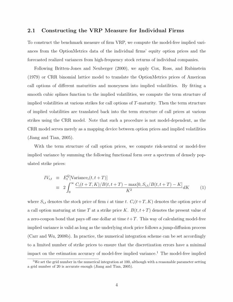
2.1 Constructing the VRP Measure for Individual Firms

To construct the benchmark measure of firm VRP, we compute the model-free implied vari-

ances from the OptionMetrics data of the individual firms’ equity option prices and the

forecasted realized variances from high-frequency stock returns of individual companies.

Following Britten-Jones and Neuberger (2000), we apply Cox, Ross, and Rubinstein

(1979) or CRR binomial lattice model to translate the OptionMetrics prices of American

call options of different maturities and moneyness into implied volatilities. By fitting a

smooth cubic splines function to the implied volatilities, we compute the term structure of

implied volatilities at various strikes for call options of T -maturity. Then the term structure

of implied volatilities are translated back into the term structure of call prices at various

strikes using the CRR model. Note that such a procedure is not model-dependent, as the

CRR model serves merely as a mapping device between option prices and implied volatilities

(Jiang and Tian, 2005).

With the term structure of call option prices, we compute risk-neutral or model-free

implied variance by summing the following functional form over a spectrum of densely pop-

ulated strike prices:

IVi,t ≡ EQt [Variancei(t, t+ T )]

≡ 2

∫ ∞0

Ci(t+ T,K)/B(t, t+ T )−max[0, Si,t/B(t, t+ T )−K]

K2dK (1)

where Si,t denotes the stock price of firm i at time t. Ci(t+T,K) denotes the option price of

a call option maturing at time T at a strike price K. B(t, t+T ) denotes the present value of

a zero-coupon bond that pays off one dollar at time t+T . This way of calculating model-free

implied variance is valid as long as the underlying stock price follows a jump-diffusion process

(Carr and Wu, 2008b). In practice, the numerical integration scheme can be set accordingly

to a limited number of strike prices to ensure that the discretization errors have a minimal

impact on the estimation accuracy of model-free implied variance.1 The model-free implied

1We set the grid number in the numerical integration at 100, although with a reasonable parameter settinga grid number of 20 is accurate enough (Jiang and Tian, 2005).

4

variance could be more informative than the implied variances using only at-the-money (out-

of-the-money or in-the-money) options, as the model-free approach incorporates the option

information across different moneyness (Jiang and Tian, 2005).

In order to define the realized variance that we use in estimating the expected variance,

let si,t denote the logarithmic stock price of firm i. The realized variance over the [t − 1, t]

time interval may be measured as:

RVi,t ≡n∑j=1

[si,t−1+ j

n− si,t−1+ j−1

n

]2−→ Variancei(t− 1, t), (2)

where the convergence relies on n→∞; i.e., an increasing number of within period price ob-

servations.2 As demonstrated in the literature (see, e.g., Andersen, Bollerslev, Diebold, and

Ebens, 2001a; Barndorff-Nielsen and Shephard, 2002), this “model-free” realized variance

measure based on high-frequency intraday data can provide much more accurate ex-post

observations of the ex-ante return variation than those based on daily data.

For a monthly horizon and monthly data frequency, where IVi,t is the end-of-month risk-

neutral expected variance for firm i of the next month, and RVi,t is the realized variance of

the current month, we adopt a linear forecast of the objective or statistical expectation of

the return variance as RVi,t+1 = α + βIVi,t + γRVi,t + εi,t+1, and the expected variance is

simply the time t forecast of realized variance from t to t+ 1 based on estimated coefficients

α̂ and β̂ in the linear regression,

EVi,t ≡ EPt [Variancei(t, t+ T )] ≡ R̂V i,t+1 = α̂ + β̂IVi,t + γ̂RVi,t, (3)

where R̂V i,t+1 is the forecasted realized variance of firm i of the next month.

We use this particular projection, because the model-free implied variance from options

market is an informationally more efficient forecast for future realized variance than the

past realized variance (see, e.g., Jiang and Tian, 2005); while realized variance based on

high-frequency data also provides additional power in forecasting future realized variance

2In practice, we use 15-minute returns, although for a similar sample of 307 US firms using 5-minutereturns produces similar quality estimation of realized variances (Zhang, Zhou, and Zhu, 2009).

5

(Andersen, Bollerslev, Diebold, and Labys, 2001b). Therefore, a joint forecast model with

one lag of implied variance and one lag of realized variance seems to capture the most

forecasting power from the time-t available information (Drechsler and Yaron, 2009).

The variance risk premium of an individual firm, or V RPi,t, underlying our key empirical

findings is defined as the difference between the ex-ante risk-neutral expectation and the

objective expectation of future return variation over the [t, t+ 1] time interval,

V RPi,t ≡ IVi,t − EVi,t. (4)

Such a construct at the market level has been shown to possess remarkable capability in

forecasting the aggregate credit spread indices (Zhou, 2009). Here we investigate in detail

how the VRP of individual firms can help us to understand the cross-section of individual

firms’ CDS spreads.

2.2 Empirical Implementation Strategy

We examine the relationship between credit default swap (CDS) spreads and variance risk

premia (VRP) in the presence of market- and firm-level credit risk determinants suggested

by theory and empirical evidence. We focus on monthly data to avoid picking up the market

microstructure noise induced by high frequency comovements between option and credit

markets. For spreads and implied variance, they are just the matched last available end-

of-month (daily) observations. Because missing dates and stale quotes signify that daily or

even weekly data quality is not reliable, and if we just ignore the daily missing values, we

will introduce serial dependent error structure in the independent variable—CDS spread,

which may artificially increase the prediction R2 or significance. Monthly data will give us

more conservative but reliable estimate and is typically the shortest horizon—compared to

quarterly or annual data—for picking up the low frequency risk premium movement.

CDS spreads should also be influenced by the leverage ratio of the underlying firm and

the risk-free spot rate. As suggested by the structural form credit risk models (Merton,

1974, and henceforth), leverage is the most important credit risk determinant—all else being

6

equal, a firm with higher leverage has a higher likelihood of default (Collin-Dufresne and

Goldstein, 2001). The leverage ratio, denoted by LEVi,t, is computed as the book value of

debt over the sum of the book value of debt and market value of equity. Moreover, structural

models predict that risk-free interest rates negatively influence the credit spread (Longstaff

and Schwartz, 1995)—when the risk-free rate is increasing, it typically signifies an improving

economic environment with better earning growth opportunity for the firms, therefore lower

default risk premium. Alternatively when short rate is rising, inflation risk is also increasing,

nominal asset debt becomes less valuable compared to real asset equity (Zhang, Zhou, and

Zhu, 2009). We define the risk-free rate variable to be the one-year swap yield, denoted by

rt.

Empirical research also shows that in practice, CDS spreads contain compensation for

non-default risks as well as risk premia which may be difficult to identify without the aggre-

gate macro variables. Henceforth, we will not limit our analysis to the traditional theoreti-

cally motivated regressors but augment our set of variables by the following market variables:

(1) the market variance risk premium based on the S&P 500 denoted by MVRPt to measure

systemic variance or macroeconomic uncertainty risk—all else equal, high market VRP leads

to high credit spreads (Zhou, 2009);3 (2) the S&P 500 return, denoted by S&Pt to proxy for

the overall state of the economy—when economy is improving the credit spread should be

lower as profit is rising (Zhang, Zhou, and Zhu, 2009); (3) Moody’s default premium slope,

denoted by DPSt, is computed as Baa yield spread minus Aaa yield spread to capture the

default risk premium in the corporate bond market—the coefficient of the default premium

slope should be positive, consistent to the notion that CDS and corporate bond markets are

cointegrated (Blanco, Brennan, and Marsh, 2005; Ericsson, Jacobs, and Oviedo, 2004; Zhu,

2006); and (4) the difference of five-year swap rate and five-year Treasury rate, denoted by

STSt, as a proxy for fixed income market illiquidity—which is expected to move positively

3The market variance risk premium is defined as the difference between the risk-neutral and objectiveexpectations of S&P 500 index variance (Zhou, 2009), where the risk-neutral expectation of variance ismeasured as the end-of-month observation of VIX-squared and the expected variance under the objectivemeasure is a forecasted realized variance with an AR(12) process. Realized variance is the sum of squared 5-minute log returns of the S&P 500 index over the month. Both variance measures are in percentage-squaredformat on monthly basis.

7

with CDS spreads (Tang and Yan, 2008).

For firm characteristic variables, besides leverage ratio, we include the following controls:

(1) asset turnover, denoted by ATOi,t, is computed as sales divided by total assets; (2) price-

earnings ratio denoted by PEi,t; (3) market-to-book ratio, denoted by MBi,t; (4) return on

assets, denoted by ROAi,t, computed as earnings divided by total assets; (5) the natural

logarithm of sales, denoted by SALEi,t. As a proxy for firm size, SALEi,t should influence

CDS spread negatively—as a larger and more mature firm tend to be investment grade

in our sample, all else being equal. Firm asset turnover, market-book ratio, and return

on assets are all expected to be negatively related to CDS spreads, because firms of high

profitability and future growth tend to have lower credit risk. Price-earnings ratio may have

two opposite effects on CDS spreads: on the one hand, high price-earnings ratio implies high

future asset growth reducing the likelihood of financial distress and credit risk; on the other

hand, high growth firms tend to have high return volatilities that increase credit risk. These

hypothesized signs of impact coefficients are consistent with the basic Merton (1974) model’s

implications and are largely confirmed by the empirical literature (e.g., see Collin-Dufresne,

Goldstein, and Martin, 2001).

Given the nature of our cross-sectional and time-series data, we adopt the robust standard

error approach of Petersen (2009) to account for both firm and time effects in large panel

data sets. Therefore, the above discussions suggest the following regression equation

CDSi,t, = α + β1V RPi,t + β2MVRPt + β3LEVi,t + β4S&Pt + β5rt

+β6DPSt + β7STSt + β8ATOi,t + β9PEi,t

+β10MBi,t + β11ROAi,t + β12SALEi,t + εi,t, (5)

and our focus is the relation between a firm’s CDS spread and its variance risk premium

(VRP).

8

3 Data Description and Summary Statistics

To conduct the empirical study, we collect data on credit default swap (CDS) spreads,

equity option prices, macroeconomic variables, firm equity and balance sheet information

from various sources. The summary statistics of CDS spreads, variance risk premia (VRP),

and other market wide or firm-specific controls, are discussed here to set the background for

examining the critical link between CDS spread and VRP.

3.1 Data Sources

Under a CDS contract, the protection seller promises to buy the reference bond at its par

value when a predefined default event occurs. In return, the protection buyer makes periodic

payments to the seller until the maturity date of the contract or until a credit event occurs.

This periodic payment, which is usually expressed as a percentage (in basis points) of the

bonds’ notional value, is called the CDS spread. By definition, credit spread provides a pure

measure of the default risk of the reference entity. We use CDS spreads as a direct measure

of credit spreads. Compared to corporate bond yield spreads, CDS spreads are not subject

to the specification of benchmark risk-free yield curve and less contaminated by non-default

risk components (Longstaff, Mithal, and Neis, 2005; Ericsson, Reneby, and Wang, 2006).

Our single-name CDS spreads are obtained from a database compiled by the Markit

group. The data set also reports average recovery rates, used by data contributors in pricing

each CDS contract, which center around 0.4 without much variations. The sample period

covers January 2001 to September 2008. We restrict our sample to US dollar denominated

CDS written on US entities that are not in the government, financial, or utility sectors. We

further eliminate the subordinated class of contracts because of its small relevance in the

database and its unappealing implications for credit risk pricing. The maturities of Markit

CDS contracts range between 6 months and 30 years. We focus on the most popular and

liquid 5-year CDS contracts with modified restructuring clauses in our benchmark analysis.

CDS spreads of other contract maturities ranging between 1- and 10-year are relatively liquid

and are used for robustness checks. After cleaning and matching the CDS data with reliable

9

option, equity and balance sheet information, we are left with more than 22,000 monthly

observations of 382 entities in our study. For each entity, the monthly CDS spreads are

matched with the monthly VRPs.

The option data is obtained from Ivy DB OptionMetrics. We keep only the options

whose last trade dates match the record dates and whose option price dates match the

underlying security price dates. We further eliminate the option prices that violate arbitrage

boundaries (C ≤ S − Ke−rTT ). Stock dividend information is acquired from CRSP and

taken into account when applying the CRR model to extract the implied volatility surface.

We compute high-frequency realized variances using information in TAQ database that

contains the intraday equity trading data spaced by 15 minutes during trading hours. Fol-

lowing the method outlined in previous section, we first calculate the daily variance based on

the high-frequency data, then aggregate it to construct monthly realized variance. Next we

estimate expected variance that is of the same maturity as the implied variance. All types

of VRPs are then matched with CDS spreads on a firm-month basis.

For market and firm control variables, they are most recently available monthly or quar-

terly variables. Firm quarterly balance-sheet data is acquired from COMPUSTAT. For

market variables, the swap rates, constant maturity Treasury yields and Moody’s Aaa and

Baa yields are acquired from the Federal Reserve Board public website. S&P 500 index

returns come from CRSP. The market VRP is from Zhou (2009).

3.2 Summary Statistics

Table 1 presents the summary statistics—average across the 382 firms—of the five-year

CDS spreads and our benchmark VRP measure (Panel A), model-free implied variances and

expected variances (Panel B). The average Moody’s and S&P ratings of the CDS reference

entities range between AAA and CCC. A majority of the CDS ratings are A, BBB and

BB (19%, 37% and 25% respectively, in total 81%). The average of CDS spreads in our

sample is 151 basis points. They increase monotonically from 17 to 603 basis points as the

credit ratings of the CDS reference entities deteriorate from AAA to CCC. The difference

between the average CDS spreads for AAA grade and AA grade is 4 basis points, whereas the

10

difference between those for CCC grade and B grade is 235 basis points. The CDS spreads

display positive skewness of around 1 and leptokurtosis of 4.44.

Similar to the CDS spreads, VRP displays significant variations across rating groups.

The average of the benchmark VRP measure for the full sample is 33 (monthly percentage

squared), increasing from 7 to 82 as CDS reference entities’ credit ratings drop from AAA

to CCC. High credit risk entities tend to be associated with high VRPs. The variance risk

premia display positive skewness of 1.2 and leptokurtosis of 5.2.

As shown in Panel B of Table 1, the means and standard deviations of model-free implied

variances are much higher than those of expected variances, but the skewness and kurtosis

are similar. It suggests that implied variance could contain a larger idiosyncratic component

than expected variance. The AR(1) coefficients for VRP, model-free implied and expected

variances are 0.38, 0.57 and 0.45 respectively, suggesting that VRP is less persistent compared

to model-free implied variances and expected variances.

We group our sample into three sub-samples by CDS ratings. The first group contains

CDS of AAA, AA and A grades, the second group contains CDS of BBB grade, and the

third group contains CDS of speculative grades ranging between BB and CCC. The three

sub-samples contain 7, 315, 9, 582 and 5, 107 firm-month observations respectively. Figure

1 plots the time-series of the five-year CDS spreads of whole sample and three sub-groups.

The CDS spreads decrease gradually from the peaks in late 2002, then increase again as

the financial crisis approaches in mid 2007. The spreads of investment grade CDS in year

2008 are higher than those in year 2002, whereas the spreads of speculative grade CDS are

lower than their 2002 level. That highlights the nature of the recent financial crisis, which

is mainly fueled by the heightening of systematic risk or economic uncertainty and affects

disproportionately the high investment grade credit spreads. The difference between the

investment grade and speculative grade CDS spreads, however, becomes widened during

2007-2008, potentially due to the “fly-to-quality” effect during the financial crisis that drives

up the compensation for credit risk.

Figure 2 further illustrates the dynamic relationships among CDS spreads, VRP, market

VRP and leverage ratio for a representative firm in our sample: General Motor (GM). The

11

CDS spread line and VRP line resemble each other closely over time. In particular, the

two lines move closely during GM downgrading in year 2005 and in the recent financial

crisis. In addition, the CDS spreads tend to comove with the firm’s leverage ratio. A

visual examination of the relationship between CDS spreads and market VRP suggests that

market risk premium, market VRP in particular, may not provide powerful prediction on

GM’s credit spreads. For instance, the two lines move in exactly opposite direction during

the period from 2004 to 2006. The market VRP line closely resembles the VIX line.

Table 2 reports the descriptive statistics for our market- and firm-level control variables—

average across 382 entities the latter. The average monthly market VRP is 22.82 (percentage-

squared). The average of one-year swap rate is 3.37%. The firms in our sample have an

average leverage ratio of 40% with a standard deviation of 6%. For simplicity, we omit

the discussion of other control variables, given that they are similar to those reported in

literature.

Table 3 reports the univariate correlations of the regression variables. It is shown that

CDS spread is positively correlated to VRP, IV and EV. Both VRP and EV are significantly

correlated to IV (0.90 and 0.95), whereas VRP and EV are much less correlated (0.73).

This suggests that VRP and EV may capture different risk components embedded in IV.

Among credit risk determinants, VRP and leverage have high correlations with CDS spreads,

whereas other variables exhibit lower correlations, suggesting that the two variables may

possess significant explanatory power for credit risk. CDS spreads are positively correlated

with market VRP’s (0.05), but the coefficients of market VRP turn out to be negative in

the presence of firm-level VRP in the multivariate regressions in the next section. The

low correlations among firm-level control variables suggest that the selected covariates well

complement each other without causing serious multicollinearity.

4 Empirical Results and Analysis

In this section, we show that firm-level variance risk premia (VRP) displays a significant

predictive power for CDS spreads in the presence of all other credit risk determinants. In

12

particular, it complements the firm leverage ratio that has been shown as the leading explana-

tory variable for credit spreads by Collin-Dufresne and Goldstein (2001) within the Merton

(1974) framework. VRP crowds out the market-level variation risk measure—market VRP—

in capturing the systematic variance risk embedded in CDS spreads. The predictive power of

VRP for CDS spreads increases as firm credit quality deteriorates. Model-free VRP performs

better than the VRP implied from call or put options of different moneyness.

Further robustness suggests that VRP and expected variance are two indispensable com-

ponents of the option-implied variance in predicting the individual firms’ credit spreads.

In addition, VRP seems to possess more forecasting power at monthly and quarter hori-

zons while implied variance more at weekly horizon, and in aggregate the market VRP

Granger-causes implied and expected variances. Finally, firm-level VRP measure contains a

systematic variance risk exposure that is priced in the cross-section of VRPs, and our result

seems to be qualitatively justifiable by simulation evidence from a structural model with

stochastic asset variance risk.

4.1 The Benchmark Regressions

Table 4 reports the regression results of the relationship between five-year CDS spreads

and benchmark VRP computed with model-free implied variance minus expected variance

estimated from lagged implied and realized variances (see Section 2). Regression 1 reports

that CDS spreads are positively related to VRP in the univariate regression. The t-statistic

is a significant 10.03. In terms of economic significance, one standard deviation increase in

VRP (21.57) will increase CDS spreads by 60 basis points, which translates into $90,000 on

a CDS contract with a notional amount of $15 million.

Regression 2 shows that including leverage ratio, as the leading determinant of credit

spread levels and changes (Collin-Dufresne and Goldstein, 2001; Collin-Dufresne, Goldstein,

and Martin, 2001), preserves the high significance of the VRP measure. As argued in theory

(Merton, 1974), when default risk increases via the leverage channel, CDS spreads increase

as well. Regression 3 shows that the relationship between CDS spreads and VRP remains

intact in the presence of market VRP. More importantly, the sign of market VRP is driven to

13

be negative, suggesting firm VRP subsumes market VRP in capturing systematic variance

risk in predicting CDS spreads. This fact remains true with the control of leverage ratio

(regression 4). As indicated in Zhou (2009), market VRP predicts a significant positive risk

premium in market credit spreads, which is consistent with our firm level evidence here.

Regression 5 reports the full-scale regression results after including all control variables.

The coefficient of VRP decreases slightly from 2.78 in the univariate regression to 2.29 but

remains statistically significant at 1 percent level with a robust t-statistic of 9.21. All the

market level control variables are statistically insignificant, except for the swap rate with

a marginal t-statistic of 1.70—when the short rate is increasing in an inflationary setting,

nominal corporate debt would be less valuable, hence the credit spread is higher. For firm-

level controls, only the negative coefficients of market-book ratio and log sales are statistically

significant at 1 percent level. The results support the intuition behind the structural-form

credit risk models in that firms with higher profitability and growth opportunity tend to

have relatively smaller chance of default hence a lower credit risk premium.

The adjusted R2 for the univariate regression indicates that 34 percent of the variation

in the CDS spreads could be accounted for by the firm specific VRP that captures firm’s

exposure to systematic uncertainty risk. Adding market VRP to the regression has very

little impact on the adjusted R2, which merely increases to 0.35. It suggests that firm-

level variation risk measure has much stronger explanatory power for individual firm’s CDS

spreads compared to the well-documented market-level variation risk measure. Including

leverage ratio in the regression increases the adjusted R2 to 0.47, possibly capturing the

firm-specific default risk on top of systematic risk in the spirit of Merton (1974). Further

adding all other control variables increases the adjusted R2 sightly to 0.49. It appears that,

among all variables, firm level VRP and leverage ratio are the two most powerful explanatory

variables affecting CDS spreads.

4.2 Robustness Checks

It is an important finding that variance risk premium (VRP) explains a significant portion of

credit risk premium, which may be orthogonal to the asset return risk that is already being

14

captured by the leverage ratio. In this section, we conduct a series of robustness checks

that such a finding is reliable if we consider different credit rating entities and is robust to

different CDS contract maturities, implied variances constructed from different options and

moneyness, and substituting market VRP control with the popular VIX index.

The credit spreads of low quality issuers are supposed to respond more to underlying

variance risk shocks captured by VRP. Therefore, we regress 5-year CDS spreads on VRP

for three sub-samples respectively: AAA-A (high investment grade), BBB (low investment

grade), and BB-CCC (speculative grade), based on the average CDS ratings of Moody’s and

S&P. We present in Table 5 both the bivariate regression results on firm VRP and leverage

ratio and the multivariate regression results on VRP with all control variables. In both sets

of regressions, the coefficients of VRP are highly significant and increase monotonically from

to as the CDS ratings deteriorate. VRP exhibits much stronger predictability on the credit

spreads of the CDS written on bonds issued by low credit quality entities. The coefficients

of VRP for the lowest rating group BB-CCC are almost five-to-seven times larger than those

for the highest rating group AAA-A and at least twice larger than those for the middle rating

group BBB, confirming our prior. Consistent with the benchmark regressions, leverage ratio

plays a significant role in affecting positively CDS spreads. The lower the credit quality of

issuing entities, the more significant impact the leverage ratio has on the CDS spreads.

We examine the relationship between CDS spreads and VRP for different CDS maturities.

Table 6 reports the regression results by CDS maturity terms: 1, 2, 3, 5, 7 and 10 years. In

all of these regressions CDS spreads are correlated positively and significantly with firm-level

VRP and leveraged ratio. The t-statistics confirms that the firm-level VRPs perform much

better than the market-level VRPs in predicting individual firm credit spreads.4 The longer

the maturity of a CDS contract, the more significant the impact of firm-level VRP on CDS

spreads with larger slope coefficients and higher adjusted R2s. It is intuitive that a CDS

contract of longer maturity is relatively exposed to a larger amount of variance uncertainty

4In another robustness check, we substitute VIX (monthly squared in percentage) for the market-levelVRP in the regressions. The unreported results show that the strong predictability of VRP on CDS spreadsremains intact in the presence of VIX. Importantly, CDS spreads are negatively and significantly correlatedto VIX. This is different from previous research that finds a positive relationship between CDS spreads andVIX (Ericsson, Reneby, and Wang, 2006) in the absence of VRP.

15

risk and requires higher spread.

To check the extent to which the significance of the explanatory power of VRP on credit

spreads depends on different methods of constructing VRP, we carry out regression analysis

of CDS spreads on VRPs constructed with various option features. Besides the benchmark

model-free implied variance, we use implied variances computed from out-of-the-money, at-

the-money and in-the-money put/call options. As reported in Table 7, all VRP measures

display consistently significant predictability for CDS spreads in the presence of other credit

risk predictors. Among them, the VRPs constructed with model-free implied variance dis-

plays the strongest predicting power on CDS spreads, reflected in both higher t-statistic

and adjusted R2. The model-free implied variance is informatively more efficient than the

implied variance from at-the-money (out-of-the-money or in-the-money) options alone as it

incorporates by construction the option information across all moneyness.

4.3 Implied Variance, Expected Variance, and VRP

Previous studies find that individual firm credit risk is strongly related to the option-implied

volatilities consistent with an argument of informational efficiency (see, e.g., Cao, Yu, and

Zhong, 2008, among others). However, in this subsection, we try to argue from several

empirically angles that the explaining power of variance risk premium (VRP) for credit

spread comes mainly from capturing a systematic risk component, tends to be long run, and

Granger-causes implied variance.

To investigate this issue, we first carry out regressions in which VRP competes against

implied variance and expected variance. Table 8 reports the results of regressing CDS spreads

on those variables. The results of regression (1)–(3) indicate that with all control variables,

VRP, implied variance, and expected variance explain 49, 52, and 48 percent of the variations

in CDS spreads respectively. In regression (4) and (5), we test the predictability of VRP

or expected variance on CDS spreads in the presence of implied variance. The coefficient

of VRP remains positive while that of expected variance turns to be negative, both are

statistically significant. In regression (6), we regress CDS spreads simultaneously on VRP

and expected variance. The coefficients of both VRP and expected variance are positive and

16

statistically significant at 1 percent level, suggesting that VRP and expected variance are

two important components in implied variance that help to explain individual firm credit

spreads.

If VRP better captures a systematic risk factor than implied variance, we might observe

that the explanatory power of VRP on CDS spreads increases as data frequency becomes

lower as systematic risk tends to be long-term. Panel A of Table 9 confirms such intuition by

showing that, in univariate regressions, the t-statistics of VRP increases monotonically from

6.44 to 10.41 as the sample frequency changes from weekly to monthly then to quarterly.

In the presence of IV in the regressions, the t-statistics of VRP increase consistently, while

the t-statistics of implied variance keep decreasing as the frequency lowers. In both sets of

regressions, the adjusted R2 increases for lower data frequency. Finally, at weekly frequency

implied variance improves the predictability of VRP by 12 percentage points; while for

monthly and quarterly frequencies only by 5 percentage points.

We apply the Granger Causality tests on market-level VRP, IV, and EV as specified in

the following regression5

Yt = φ+m∑i=1

κiXt−i +n∑j=1

θjYt−j + εt (6)

and the null hypothesis is κ = 0. We set both m and n equal 3.6 We find evidence that VRP

significantly Granger causes both IV and EV, but not vise versa. Panel B of Table 9 shows

that IV and EV are significantly correlated with VRP lags, while VRP is not significantly

explained by either lag IV or lag EV. The results suggest that, being potentially a cleaner

measure of systematic risk, VRP helps to predict future variations in IV and EV that are

more likely to be contaminated with idiosyncratic risks.

We carry out the Principal Components Analysis on VRP, IV and EV. As reported in

Table 10, the first principle component explains 78 percent of the total variation in VRP,

5We also perform the Granger Causality tests on individual firms’ VRP, IV, and EV. The results arenoisy and insignificant, which cannot support any clean causality pattern.

6The selection of number of lags in a Granger Causality test balances the trade-off between eliminatingautocorrelation in residual and maintaining testing power. We report the results with m,n = 3 since theregression R2s stop changing significantly at three lags.

17

while it only explains 54 percent in implied variance. And the first four principal components

cumulatively explains 95 percent of VRP variation versus only 75 percent of implied variance.

In other words, VRP is likely a cleaner measure of firms’ exposure to systematic variance

or economic uncertainty risk relative to the implied variance or expected variance, which

is consistent with the finding that a missing systematic risk factor may hold the key for

explaining the credit spread puzzle(s) (Collin-Dufresne, Goldstein, and Martin, 2001).

4.4 Cross-Sectional Validation of Market VRP

To examine to what extent firm-level VRP captures the exposure to a systematic variance

risk factor, we compare the relationship between firm and market VRPs to the relationship

between firm and market equity returns with the matched sample. Following the standard

approach of testing CAPM (e.g., Lintner, 1965), we carry out two-stage regressions. In the

first stage, we run time-series regressions for each firm i to estimate its βV RPi and βCAPMi ,

respectively: V RPit = αV RPi + βV RPi × V RPMKT

t + εit

Rit = αCAPMi + βCAPMi ×RMKTt + εit,

(7)

We then compute each firm’s average VRP, V RPi, and average equity return, Ri, respectively.

The second-stage cross-sectional regressions are as following:V RPi = λV RP0 + λV RP1 × β̂V RP i + εi

Ri = λCAPM0 + λCAPM1 × β̂CAPMi + εi.

(8)

The fundamental hypotheses being tested are λV RP0 = 0, λV RP1 = Mean Market VRP;

λCAPM0 = 0, λCAPM1 = Mean Market Return.

Panel A of Table 11 reports the summary statistics of βV RPi and βCAPMi . As indicated

by percentile, the t-statistics of βV RPi are relatively more dispersively distributed and more

significant in the percentiles between 50% and 99%. In addition, the R2s of the VRP regres-

sions are generally higher than their counterparts in the CAPM regressions. The evidence

18

suggests that VRP captures systematic risk more strongly than the well documented equity

returns do. The means of the t-statistics for VRP and equity return regressions are 4.29

and 3.91, respectively. The difference is on average 0.38 with a standard deviation of 0.18.

Unreported mean comparison t-test shows a t-statistic of 2.15, indicating the t-statistic of

the VRP regressions are statistically higher than that of the equity return regressions.

Panel B shows that VRP is significantly related to βV RP with a t-statistic of 7.51, but

equity return is not significantly related to βCAPM . The VRP regression has an adjusted R2

of 14.05 percent, compared to an adjusted R2 of zero for the equity return regression.7 Figure

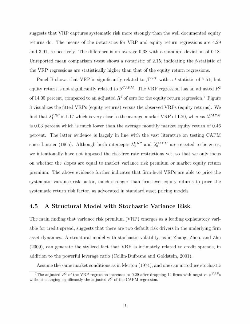
3 visualizes the fitted VRPs (equity returns) versus the observed VRPs (equity returns). We

find that λV RP1 is 1.17 which is very close to the average market VRP of 1.20, whereas λCAPM1

is 0.03 percent which is much lower than the average monthly market equity return of 0.46

percent. The latter evidence is largely in line with the vast literature on testing CAPM

since Lintner (1965). Although both intercepts λV RP0 and λCAPM0 are rejected to be zeros,

we intentionally have not imposed the risk-free rate restrictions yet, so that we only focus

on whether the slopes are equal to market variance risk premium or market equity return

premium. The above evidence further indicates that firm-level VRPs are able to price the

systematic variance risk factor, much stronger than firm-level equity returns to price the

systematic return risk factor, as advocated in standard asset pricing models.

4.5 A Structural Model with Stochastic Variance Risk

The main finding that variance risk premium (VRP) emerges as a leading explanatory vari-

able for credit spread, suggests that there are two default risk drivers in the underlying firm

asset dynamics. A structural model with stochastic volatility, as in Zhang, Zhou, and Zhu

(2009), can generate the stylized fact that VRP is intimately related to credit spreads, in

addition to the powerful leverage ratio (Collin-Dufresne and Goldstein, 2001).

Assume the same market conditions as in Merton (1974), and one can introduce stochastic

7The adjusted R2 of the VRP regression increases to 0.29 after dropping 14 firms with negative βV RP swithout changing significantly the adjusted R2 of the CAPM regression.

19

variance into the underlying firm-value process:

dAtAt

= (µ− δ)dt+√VtdW1t, (9)

dVt = κ(θ − Vt)dt+ σ√VtdW2t, (10)

where At is the firm value, µ is the instantaneous asset return, and δ is the asset payout

ratio. The asset return variance, Vt, follows a square-root process with long-run mean θ,

mean reversion κ, and volatility-of-volatility parameter σ. Finally, the correlation between

asset return and return volatility is corr (dW1t, dW2t) = ρ.

With proper bankruptcy assumptions, we can solve the equity price, St, as a European

call option on firm asset At with maturity T : St = AtF∗1 − Be−r(T−t)F ∗2 , with r being the

risk-free rate. F ∗1 and F ∗2 are the so-called risk-neutral probabilities. Therefore, the debt

value can be expressed as Dt = At − St, and its price is Pt = Dt/B, where B is the face

value of debt. The credit spread, CSt, is given by:

CSt = − 1

T − tlog(Pt)− r. (11)

The structural credit risk model presented here also implies the following equity variance

process, V st =

(At

St

)2 (∂St

∂At

)2Vt +

(σSt

)2 (∂St

∂Vt

)2Vt + At

S2t

∂St

∂At

∂St

∂VtρσVt . Inside simulation, we can

examine the relationship between credit spread CSt and VRP

V RPt = EQt (RVt+1)− EP

t (RVt+1) (12)

where RVt+1 is the realized variance from five-minute equity returns, and the risk-neutral

expectation EQt (·) and physical expectation EP

t (·) are approximated using the asset volatility

dynamics (10).

Using a calibrated parameter setting for a BBB firm as in Zhang, Zhou, and Zhu (2009),

we simulate 60 month of data of credit spreads, VRP, expected variance, and leverage ratio

for both a Merton (1974) model and a stochastic volatility model (as above). Table 12

report the OLS regressions on explaining credit spreads with those proxies for underlying

risk factors in asset value and volatility dynamics.

20

For the Merton (1974) model, leverage ratio will drive expected variance to be statistically

insignificant, even though variance itself has a significant positive effect on credit spread.

Note that for Merton model, although the asset volatility is constant, the equity volatility

is time-varying; because asset value is time-varying and equity volatility is approximately

leverage adjusted asset volatility. Therefore equity volatility does explain credit spread, but

its effect is mostly subsumed when leverage ratio is included in the regression.

However, for the two factor stochastic volatility model, not only expected variance, VRP,

and leverage ratio all have significant positive effect on credit spreads; but also any two

variables combined together would both remain statistically significant with positive signs.

In particular, the powerful leverage ratio cannot crowd out VRP or expected variance. This

is due to the fact that both asset value and asset volatility are time-varying priced risk

factors, and VRP or expected variance is not redundant to leverage ratio as in the case of

one-factor Merton (1974) model. This result is qualitatively consistent with what we have

discovered here for a large cross-section of individual firms’ CDS spreads and VRPs.

5 Conclusions

Investors demand variance risk premium (VRP) as a compensation for firms’ exposures to a

systematic factor. Such a risk premium may arise from the time-varying fluctuations in the

underlying cash flow or consumption volatility (Bansal and Yaron, 2004; Bollerslev, Tauchen,

and Zhou, 2009). Recent studies suggest that market VRP captures the macroeconomic

uncertainty or systematic variance risk that constitute a critical component in explaining

the aggregate credit spread indices (Zhou, 2009; Buraschi, Trojani, and Vedolin, 2009).

In this paper we carry out a comprehensive investigation on the relationship between the

firm-level VRPs and credit spreads, and justify empirically that VRP provides a risk-based

explanation for the credit spread variations.

We illustrate that VRPs of individual firms, estimated by the difference between model-

free implied and expected variances, possess a significant explanatory power for credit default

swap (CDS) spreads. Importantly, such predictability cannot be substituted for by that

21

of market- and firm-level credit risk factors identified in previous research. In addition,

firm-level VRP dominates the well-documented market-level VRP or VIX in capturing the

macroeconomic uncertainty or systematic variance risk premium embedded in CDS spreads.

The predictive power of VRP increases as the credit quality of CDS entities deteriorates and

as the maturity of CDS contract increases. Leverage ratio and VRP emerge as two leading

predictors of firms’ credit spreads, pointing to asset value and stochastic volatility as two

underlying risk drivers.

Empirical evidence also suggests that the superior explanatory power of VRP for CDS

spreads tends to be stronger over monthly and quarterly horizons, while that of implied

variance over weekly horizon. Also, the aggregate VRP seems to Granger-causes implied

and expected variances, but not vise versa. A principle component analysis indicates that

firms’ VRPs have a much larger systematic component relative to implied and expected

variances. These additional findings imply that firms’ VRP may be a good measure of

exposure to a systemic variance risk or economic uncertainty factor, which is consistent

with the fact that the cross-section of firm’s VRPs can be used to validate the market VRP

correctly. Further more, the stylized predictability pattern of VRP for credit spread can be

reproduced in simulation by a structural model with stochastic variance.

22

References

Andersen, Torben G., Tim Bollerslev, Francis X. Diebold, and Heiko Ebens (2001a), “The

Distribution of Realized Stock Return Volatility,” Journal of Financial Economics , vol. 61,

43–76.

Andersen, Torben G., Tim Bollerslev, Francis X. Diebold, and Paul Labys (2001b), “The

Distribution of Realized Exchange Rate Volatility,” Journal of the American Statistical

Association, vol. 96, 42–55.

Bansal, Ravi and Amir Yaron (2004), “Risks for the Long Run: A Potential Resolution of

Asset Pricing Puzzles,” Journal of Finance, vol. 59, 1481–1509.

Barndorff-Nielsen, Ole and Neil Shephard (2002), “Econometric Analysis of Realised Volatil-

ity and Its Use in Estimating Stochastic Volatility Models,” Journal of Royal Statistical

Society Series B , vol. 64, 253–280.

Berndt, Antj, Aziz A. Lookman, and Iulian Obreja (2006), “Default Risk Premia and Asset

Returns,” Carnegie Mellon University, Working Paper.

Bhamra, Harjoat, Lars-Alexander Kuhn, and Ilya Strebulaev (2009), “The Levered Equity

Risk Premium and Credit Spreads: A United Framework,” Standford University, Working

Paper.

Blanco, Roberto, Simon Brennan, and Ian Marsh (2005), “An Empirical Analysis of the Dy-

namic Relationship Between Investment-Grade Bonds and Credit Default Swaps,” Journal

of Finance, vol. 60, 2255–2281.

Bollerslev, Tim, George Tauchen, and Hao Zhou (2009), “Expected Stock Returns and

Variance Risk Premia,” Review of Financial Studies,” Review of Financial Studies , vol. 22,

4463–4492.

Britten-Jones, Mark and Anthony Neuberger (2000), “Option Prices, Implied Price Processes

and Stochastic Volatility,” Journal of Finance, vol. 55, 839–866.

Buraschi, Andrea, Fabio Trojani, and Andrea Vedolin (2009), “The Joint Behavior of Credit

Spreads, Stock Options and Equity Returns When Investors Disagree,” Imperial College

London Working Paper.

Campbell, John Y. and Glen B. Taksler (2003), “Equity Volatility and Corporate Bond

Yields,” Journal of Finance, vol. 58, 2321–2349.

Cao, Charles, Fan Yu, and Zhaodong Zhong (2008), “How Important Is Option-Implied

Volatility for Pricing Credit Default Swaps,” Forthcoming.

23

Carr, Peter and Liuren Wu (2008a), “Stock Options and Credit Default Swaps: A Joint

Framework for Valuation and Estimation,” New York University, Working Paper.

Carr, Peter and Liuren Wu (2008b), “Variance Risk Premia,” Review of Financial Studies ,

vol. 22, 1311–1341.

Chen, Hui (2009), “Macroeconomic Conditions and the Puzzles of Credit Spreads and Capital

Structure,” Journal of Finance, page forthcoming.

Chen, Long, Pierre Collin-Dufresne, and Robert Goldstein (2009), “On the Relation Between

the Credit Spread Puzzle and the Equity Premium Puzzle,” Review of Financial Studies ,

vol. 22, 3367–3409.

Collin-Dufresne, Pierre and Robert Goldstein (2001), “Do Credit Spreads Reflect Stationary

Leverage Ratios?” Journal of Finance, vol. 56, 1929–1957.

Collin-Dufresne, Pierre, Robert S. Goldstein, and Spencer Martin (2001), “The Determinants

of Credit Spread Changes,” Journal of Finance, vol. 56, 2177–2207.

Cox, John, Stephen Ross, and Mark Rubinstein (1979), “Option Pricing: A simplified ap-

proach,” Journal of Financial Economics , vol. 7, 229–263.

Cremers, Martijn, Joost Driessen, Pascal Maenhout, and David Weinbaum (2008), “Individ-

ual Stock-Option Prices and Credit Spreads,” Journal of Banking and Finance, vol. 32,

2706–2715.

David, Alexander (2008), “Inflation Uncertainty, Asset Valuations, and the Credit Spread

Puzzles,” Reveiew of Financial Studies , vol. 21, 2487–2534.

Drechsler, Itamar and Amir Yaron (2009), “What’s Vol Got to Do With It.” University of

Pennsylvania, Working Paper.

Elton, Edwin, Martin Gruber, Deepak Agrawal, and Christopher Mann (2001), “Explaining

the Rate Spread on Corporate Bonds,” Journal of Finance, vol. 56, 247–277.

Ericsson, Jan, Kris Jacobs, and Rodolfo Oviedo (2004), “The Determinants of Credit Default

Swap Premia,” McGill University, Working Paper.

Ericsson, Jan, Joel Reneby, and Hao Wang (2006), “Can Structural Models Price Default

Risk? Evidence from Bond and Credit Derivative Markets,” McGill University, Working

Paper.

24

Huang, Jing-Zhi and Ming Huang (2003), “How Much of the Corporate-Treasury Yield

Spread is Due to Credit Risk? A New Calibration Approach,” Pennsylvania State Uni-

versity, Working paper.

Jiang, George and Yisong Tian (2005), “The Model-Free Implied Volatility and Its Informa-

tion Content,” Review of Financial Studies , vol. 18, 1305–1342.

Jones, Philip, Scott Mason, and Eric Rosenfeld (1984), “Contingent Claims Analysis of

Corporate Capital Structures: An Empirical Investigation,” Journal of Finance, vol. 39,

611–627.

Lintner, John (1965), “Security Prices, Risk and Maximal Gains from Diversification,” Jour-

nal of Finance, vol. 20, 587–615.

Longstaff, Francis, Sanjay Mithal, and Eric Neis (2005), “Corporate Yield Spreads: Default

Risk or Liquidity? New Evidence from the Credit Default Swap Market,” Journal of

Finance, vol. 60, 2213–2253.

Longstaff, Francis and Eduardo Schwartz (1995), “Valuing Credit Derivatives,” Journal of

Fixed Income, vol. June, 6–12.

Merton, Robert (1974), “On the Pricing of Corporate Debt: The Risk Structure of Interest

Rates,” Journal of Finance, vol. 29, 449–479.

Petersen, Mitchell (2009), “Estimating Standard Errors in Finance Panel Data Sets: Com-

paring Approaches,” Review of Financial Studies , vol. 22, 435–480.

Tang, Dragon Yongjun and Hong Yan (2008), “Liquidity, Liquidity Spillovers, and Credit

Default Swap Spreads,” University of Hong Kong, Working Paper.

Zhang, Benjamin, Hao Zhou, and Haibin Zhu (2009), “Explaining Credit Default Swap

Spreads with the Equity Volatility and Jump Risks of Individual Firms,” Review of Fi-

nancial Studies , vol. 22, 5099–5131.

Zhou, Hao (2009), “Variance Risk Premia, Asset Predictability Puzzles, and Macroeconimc

Uncertainty,” Federal Reserve Board, Working Paper.

Zhu, Haibin (2006), “An Empirical Comparison of Credit Spreads Between the Bond Market

and the Credit Default Swap Market,” Bank of International Settlements, Working Paper.

25

Tab

le1:

Desc

rip

tive

Sta

tist

ics

-C

DS

Spre

ads,

Vari

ance

Ris

kP

rem

ium

,Im

pli

ed

Vari

ance

and

Exp

ect

ed

Vari

ance

.T

his

tab

lep

rese

nts

the

sum

mar

yst

atis

tics

—av

erag

eac

ross

the

382

firm

s—of

the

five

-yea

rC

DS

spre

ads

and

our

ben

chm

ark

Var

ian

ce

Ris

kP

rem

ium

(VR

P)

mea

sure

(Pan

elA

),m

od

el-f

ree

imp

lied

vari

ance

san

dex

pec

ted

vari

ance

s(P

anel

B).

Th

eC

DS

spre

ads

are

inb

asis

poin

ts.

Th

eV

RP

isco

mp

ute

das

the

spre

adb

etw

een

mod

el-f

ree

imp

lied

vari

ance

and

exp

ecte

dva

rian

ce.

Th

eim

pli

edva

rian

ceis

the

mod

el-f

ree

imp

lied

vari

an

ce.

Th

eex

pec

ted

vari

ance

isth

eli

nea

rfo

reca

stof

real

ized

vari

ance

by

lagg

edim

pli

edan

dre

aliz

edva

rian

ce.

Th

eav

erage

Mood

y’s

and

S&

Pra

tin

gs

of

the

CD

Sre

fere

nce

enti

ties

ran

geb

etw

een

AA

Aan

dC

CC

.T

he

nu

mb

ers

offi

rms

inea

chra

tin

g

cate

gory

are

rep

orte

din

the

seco

nd

colu

mn

inP

anel

A.

AR

(1)

den

otes

auto

corr

elat

ion

wit

hon

ela

g.

Pan

elA

:T

he

mea

ns

ofth

est

atis

tics

ofC

DS

spre

ads

and

VR

Pac

ross

indiv

idual

firm

s

CD

SS

pre

adV

RP

Rat

ing

Fir

mN

um

ber

Mea

nS

DS

kew

.K

urt

.A

R(1

)M

ean

SD

Skew

.K

urt

.A

R(1

)

AA

A7

17.4

312

.04

1.54

5.92

0.88

7.34

9.08

1.59

6.87

0.46

AA

17

20.9

710

.29

0.97

3.62

0.87

10.1

611

.03

2.00

9.01

0.40

A101

33.8

418

.18

1.33

4.98

0.86

16.9

715

.43

1.46

5.86

0.52

BB

B199

77.0

739

.06

1.10

4.41

0.84

23.2

317

.81

1.23

5.25

0.37

BB

133

220.

8085

.26

0.90

4.84

0.74

43.7

125

.87

1.05

4.67

0.35

B65

368.

4411

9.56

0.39

2.98

0.66

63.8

935

.73

0.88

4.08

0.24

CC

C14

603

.10

237.

080.

693.

570.

6082

.03

39.7

80.

162.

940.

31

Tota

l382

151.

1858

.94

1.01

4.44

0.80

32.8

021

.57

1.20

5.20

0.38

Pan

elB

:T

he

mea

ns

ofth

est

atis

tics

ofIV

and

EV

acro

ssin

div

idual

firm

sIm

pli

edV

aria

nce

Exp

ecte

dV

aria

nce

Rati

ng

Mea

nS

DS

kew

.K

urt

.A

R(1

)M

ean

SD

Ske

w.

Ku

rt.

AR

(1)

AA

A40.3

827.

391.

757.

230.

6533

.04

18.7

01.

106.

710.

65

AA

45.

9827

.08

1.72

6.92

0.60

35.8

217

.22

1.62

6.41

0.52

A66

.90

37.4

51.

445.

440.

6649

.93

23.2

11.

435.

320.

58

BB

B88.

1441.

431.

215.

040.

5864

.91

25.5

61.

224.

990.

50

BB

144.

2256

.45

1.13

4.86

0.54

100.

5133

.68

1.12

4.85

0.32

B193

.06

72.3

01.

014.

230.

5112

9.17

41.3

61.

004.

210.

28

CC

C234

.52

69.0

00.

533.

620.

4115

2.49

36.3

30.

503.

620.

31

Tota

l11

2.1

847.

891.

225.

050.

5779

.38

28.8

01.

224.

220.

45

26

Table 2 Summary Statistics - the Market and Firm Characteristic Variables.This table reports the descriptive statistics of the market- and firm-level control variables. For firm

characteristics, we report the averages of the statistics across 382 firms. The market VRP is the

difference between implied variance and expected variance of the S&P 500 index as in Bollerslev,

Tauchen and Zhou (2009). The S&P 500 return, is the proxy for the overall state of the economy.

The one year swap rate is the proxy for the risk-free interest rate. The Moody’s default premium

slope, defined as Baa yield spread minus Aaa yield spread is the default risk premium in the

corporate bond market. The difference of five-year swap rate and five-year Treasury rate is a proxy

for fixed income market illiquidity. The asset turnover is computed as sales divided by total assets.

The price-earnings ratio is the ratio of price over earnings. The market-to-book ratio is the ratio of

market equity to book equity. The return on assets is computed earnings divided by total assets.

AR(1) denotes autocorrelation with one lag.

Variable Mean SD Skewness Kurtosis AR(1)

Market Level

Market VRP (%) 22.82 21.92 2.88 12.32 0.27

S&P 500 Return (%) −0.02 1.98 −0.17 4.15 −0.17

Swap (1 year, %) 3.37 1.47 0.06 1.56 0.98

Baa - Aaa (%) 0.99 0.22 0.64 2.36 0.95

Swap - CMT (5 year, %) 0.54 0.16 0.85 2.68 0.90

Firm Level

Leverage Ratio 0.40 0.06 0.37 2.88 0.89

Asset Turnover (%) 1.09 0.15 0.09 3.00 0.79

Price-earnings Ratio 16.26 53.55 0.23 8.06 0.76

Market/Book Ratio 2.12 10.42 0.27 3.57 0.85

Return on Assets (%) 5.69 6.51 −0.67 7.89 0.69

Annualized Sales ($ billion) 14.30 3.16 0.25 2.74 0.87

Firm Assets ($ billion) 16.15 3.28 0.17 2.85 0.94

27

Tab

le3:

Univ

ari

ate

Corr

ela

tions

of

the

Regre

ssio

nV

ari

able

sT

his

tab

lere

por

tsth

eu

niv

ari

ate

corr

elat

ion

sof

the

regr

essi

onva

riab

les.CDS

den

otes

five

-yea

rm

atu

rity

CD

Ssp

read

.V

RP

den

otes

firm

leve

lva

rian

ceri

skp

rem

ium

con

stru

cted

wit

hm

od

elfr

eeim

pli

edva

rian

ceIV

min

us

exp

ecte

dva

rian

ceEV

esti

mat

edw

ith

hig

hfr

equ

ency

equ

ity

retu

rns.MVRP

rep

rese

nts

mark

etva

rian

ceri

skp

rem

ium

.S

&P

andr

den

ote

S&

P50

0re

turn

and

swap

rate

ofon

e-yea

rm

atu

rity

resp

ecti

vely

.DPS

rep

rese

nts

def

ault

risk

pre

miu

mm

easu

red

asth

esp

read

bet

wee

nM

ood

y’sBaa

andAaa

rate

s.STS

isth

esp

read

bet

wee

nfi

ve-

year

swap

and

con

stan

tm

atu

rity

Tre

asu

ryra

tes.LEV

den

otes

mar

ket

leve

rage

.ATO

,PE

,MB

andROA

den

ote

asse

t

turn

over

,p

rice

-earn

ings

rati

o,

mark

et-b

ook

rati

oan

dre

turn

onas

sets

resp

ecti

vely

.SALE

isth

en

atu

ral

loga

rith

mof

annual

sale

s.

CDS

VRP

IV

EV

MVRP

S&P

rDPS

STS

LEV

ATO

PE

MB

ROA

SALE

CDS

1.00

VRP

0.58

1.00

IV

0.62

0.90

1.0

0

EV

0.57

0.73

0.9

51.0

0

MVRP

0.05

0.26

0.2

90.2

81.

00

S&P−

0.0

2−

0.0

2−

0.0

2−

0.0

20.

171.

00

r−

0.08

−0.

18−

0.17

−0.

14−

0.32

−0.

061.

00

DPS

0.11

0.23

0.2

80.2

90.

35−

0.10

−0.

331.

00

STS

0.07

0.18

0.2

60.2

80.

27−

0.14

0.15

0.50

1.00

LEV

0.52

0.29

0.3

20.3

00.

050.

00−

0.09

0.06

0.02

1.00

ATO−

0.06

−0.

03−

0.01

0.01

−0.

01−

0.01

0.02

−0.

000.

01−

0.05

1.00

PE−

0.0

3−

0.0

3−

0.0

4−

0.0

4−

0.01

0.01

0.01

−0.

01−

0.00

−0.

030.

001.

00

MB−

0.0

20.0

0−

0.0

1−

0.0

10.

00−

0.00

−0.

020.

00−

0.00

−0.

02−

0.00

0.00

1.00

ROA−

0.28

−0.

22−

0.23

−0.

20−

0.04

−0.

020.

06−

0.03

−0.

01−

0.42

0.10

0.03

0.02

1.00

SALE−

0.1

7−

0.1

8−

0.2

0−

0.1

90.

040.

00−

0.01

0.04

0.06

0.01

0.38

−0.

010.

010.

091.

00

28

Table 4 The CDS Spreads and VRPThis table reports the regression results of five-year CDS spreads on the VRP computed with

model free implied variance IV minus expected variance EV estimated with high frequency equity

returns. Regression (1) is for the univariate regression; regression (2) shows the relationship between

CDS spreads and VRP in the presence of firm leverage only; regression (3) shows the relationship

between CDS spreads and VRP in the presence of market VRP (monthly squared in percentage)

only; regression (4) further includes firm leverage into regression (3); and regression (5) includes

all other control variables. We adjust two-dimensional (firm and time) clustered standard errors in

the regressions as in Petersen (2009). The numbers in the brackets are t-statistics.

Regression

Independent Variable (1) (2) (3) (4) (5)

VRP 2.78 2.26 2.92 2.38 2.29

(10.03) (11.00) (10.04) (11.06) (9.21)

Leverage 3.29 3.27 3.27

(8.89) (9.05) (8.60)

Market VRP −1.12 −1.03 −0.94

(−4.38) (−4.48) (−4.34)

S&P 500 Return 0.57

(0.48)

Swap Rate (1 Year) 2.69

(1.70)

Baa − Aaa 17.04

(1.09)

Swap Rate − CMT (5 Year) −9.62

(−0.43)

Asset Turnover Ratio 3.09

(0.59)

Price-earnings Ratio −0.01

(−1.05)

Market/Book Ratio −0.02

(−2.79)

Return on Assets −23.56

(−0.92)

Log Sales −12.23

(−3.06)

Constant 28.00 −84.68 41.20 −71.82 −0.31

(5.89) (−5.67) (10.46) (−5.52) (−0.01)

Adjusted R2 0.34 0.47 0.35 0.48 0.49

29

Table 5 CDS Spreads and VRP by CDS RatingsThis table reports the regression results of CDS spreads on VRP for three sub-samples: AAA-A,

BBB, BB-CCC. The ratings are the average of Moody’s and S&P ratings. Two-dimensional (firm

and time) clustered standard errors in the regressions are adjusted as in Petersen (2009). The group

AAA-A has 7315 observations. The group BBB has 9582 observations. The group BB-CCC has

5107 observations. The first three regressions are the regressions of VRPs and leverage. The second

three regressions are the multivariate regressions with all the control variables. The numbers in the

brackets are t-statistics.

Regression By Ratings

Independent Variable AAA-A BBB BB-CCC AAA-A BBB BB-CCC

VRP 0.48 1.06 2.20 0.29 0.81 2.12

(9.58) (10.30) (9.46) (8.02) (7.34) (7.71)

Leverage 0.44 1.19 5.84 0.40 1.10 5.76

(5.33) (6.37) (6.47) (5.71) (5.38) (6.62)

Market VRP −0.01 0.12 −0.60

(−0.28) (1.26) (1.13)

S&P 500 Return −0.01 −0.10 0.22

(−0.04) (−0.15) (0.09)

Swap Rate (1 Year) −2.35 −2.79 −5.62

(−5.33) (−2.86) (−1.38)

Baa − Aaa 20.48 34.40 70.29

(6.33) (3.72) (1.57)

Swap Rate − CMT (5 Year) 39.26 30.29 −51.11

(6.51) (2.07) (−1.02)

Asset Turnover Ratio 3.05 6.00 −36.62

(2.82) (1.63) (−2.26)

Price-earnings Ratio −0.00 −0.00 −0.01

(−1.56) (−0.14) (−0.54)

Market/Book Ratio −0.00 −0.17 −0.02

(−0.35) (1.07) (−4.29)

Return on Assets −13.42 −57.29 −9.18

(−1.33) (−2.85) (−0.28)

Log Sales −4.29 −6.14 8.01

(−6.00) (−1.82) (0.85)

Constant 10.12 −0.38 −137.35 15.11 11.00 −166.68

(4.62) (−0.05) (−2.94) (2.50) (0.49) (0.02)

Adjusted R2 0.30 0.30 0.46 0.50 0.35 0.47

30

Table 6 The CDS Spreads of Different Maturity Terms and VRPThis table reports the regression results of CDS spreads of all maturities on the VRP computed with

model free implied variance IV minus expected variance EV estimated with high frequency equity

returns. We adjust two-dimensional (firm and time) clustered standard errors in the regressions as

in Petersen (2009). The numbers in the brackets are t-statistics.

CDS Spreads

Independent Variable 1-year 2-year 3-year 5-year 7-year 10-year

VRP 1.92 2.14 2.28 2.29 2.32 2.34

(7.55) (7.39) (8.55) (9.21) (9.16) (9.25)

Leverage 2.08 2.44 2.81 3.27 3.27 3.34

(6.09) (6.13) (7.18) (8.60) (8.75) (9.11)

Market VRP −0.56 −0.78 −0.85 −0.94 −0.96 −0.91

(−3.01) (−3.56) (−3.88) (−4.34) (−4.18) (−3.82)

S&P 500 Return 0.68 0.76 0.79 0.57 0.44 0.31

(0.88) (0.80) (0.77) (0.48) (0.34) (0.23)

Swap Rate (1 Year) −7.89 −4.69 −2.71 2.69 6.92 9.89

(−6.03) (−3.36) (−1.89) (1.70) (3.96) (5.37)

Baa − Aaa 12.27 12.36 15.10 17.04 15.50 8.53

(0.82) (0.75) (0.98) (1.09) (0.95) (0.51)

Swap Rate − CMT (5 Year) −44.49 −31.33 −24.29 −9.62 −3.07 2.63

(−2.74) (−1.58) (−1.23) (−0.43) (−0.14) (0.11)

Asset Turnover Ratio −2.87 −3.61 −1.01 3.10 3.40 4.50

(−0.69) (−0.74) (−0.20) (0.59) (0.63) (0.84)

Price-earnings Ratio −0.00 −0.00 −0.01 −0.01 −0.01 −0.00

(−0.14) (−0.27) (−0.67) (−1.05) (−0.99) (−0.66)

Market/Book Ratio −0.01 −0.01 −0.01 −0.02 −0.02 −0.03

(−1.42) (−2.62) (−2.26) (2.79) (−3.30) (−3.38)

Return on Assets −7.75 −15.25 −16.24 −23.56 −30.56 −33.55

(−0.35) (−0.57) (−0.61) (−0.92) (−1.22) (−1.37)

Log Sales −2.59 −3.33 −6.51 −12.23 −12.68 −14.59

(−0.76) (−0.88) (−1.63) (−3.06) (−3.13) (−3.64)

Constant −1.92 −18.96 −14.66 −0.31 −6.59 6.38

(−0.07) (−0.66) (−0.48) (−0.01) (−0.21) (0.20)

Adjusted R2 0.40 0.41 0.46 0.49 0.50 0.51

31

Table 7 CDS Spreads and VRPs of Different Implied VariancesThis table reports the regression results of CDS spreads on VRPs computed from different measures

of implied variances. Besides the benchmark VRP computed from model-free implied variance, we

use VRP constructed from implied variances of out-of-the-money (OTM), at-the-money (ATM) and

in-the-money (ITM) put options, together with those of out-of-the-money (OTM), at-the-money

(ATM) and in-the-money (ITM) call options. We adjust two-dimensional (firm and time) clustered

standard errors in the regressions as in Petersen (2009). The numbers in the brackets are t-statistics.

VRP constructed with implied variance from

Model-Free Put Option Call Option

Independent Variable OTM ATM ITM OTM ATM ITM

VRP 2.29 1.56 2.62 1.22 1.44 2.53 1.49

(9.21) (7.72) (7.50) (6.70) (7.21) (7.74) (7.46)

Leverage 3.27 3.62 3.46 3.89 3.71 3.61 3.64

(8.60) (8.78) (9.47) (8.16) (7.75) (9.01) (8.72)

Market VRP −0.94 −1.04 −1.03 −0.50 −0.40 −0.91 −0.97

(−4.34) (−4.37) (−4.19) (−3.05) (−3.07) (−4.26) (−4.18)

S&P 500 Return 0.57 0.94 0.14 −0.87 0.23 0.97 1.21

(0.48) (0.74) (0.10) (−0.89) (0.26) (0.81) (0.98)

Swap Rate (1 Year) 2.69 2.65 1.24 −1.94 0.02 1.04 2.55

(1.70) (1.64) (0.79) (−1.42) (0.01) (0.69) (1.61)

Baa - Aaa 17.04 3.12 15.82 37.44 40.29 16.41 5.04

(1.09) (0.18) (0.98) (3.00) (3.32) (1.05) (0.30)

Swap Rate - CMT (5 Year) −9.62 15.24 5.66 18.27 32.76 14.81 14.96

(−0.43) (0.69) (0.25) (1.01) (1.92) (0.69) (0.69)

Asset Turnover Ratio 3.09 6.15 6.67 10.30 6.26 7.82 6.08

(0.59) (1.13) (1.29) (1.76) (1.06) (1.47) (1.10)

Price-earnings Ratio −0.01 −0.01 −0.01 −0.02 −0.02 −0.01 −0.01

(−1.05) (−1.31) (−1.38) (−1.62) (−1.78) (−1.39) (−1.30)

Market/Book Ratio −0.02 −0.02 −0.02 −0.01 −0.01 −0.02 −0.02

(−2.79) (−4.30) (−2.87) (−2.68) (−2.81) (−2.75) (−4.21)

Return on Assets −23.56 −46.95 −34.92 −67.76 −76.59 −41.86 −50.54

(−0.92) (−1.80) (−1.41) (−2.46) (−2.86) (−1.62) (−1.92)

Log Sales −12.23 −19.88 −17.33 −22.03 −16.20 −19.11 −20.06

(−3.06) (−5.14) (−4.54) (−5.53) (−3.83) (−5.03) (−5.18)

Constant −0.31 −19.88 34.08 55.99 3.62 42.76 50.47

(−0.01) (−5.14) (1.18) (1.77) (0.10) (1.45) (1.68)

Adjusted R2 0.49 0.44 0.48 0.38 0.37 0.45 0.43

32

Table 8 VRP Versus Implied Variance and Expected Variance.This table compares the predictability of VRP on CDS spreads to that of model-free implied and

expected variances for 5-year maturity CDS spreads. Regression (1) to (3) report the multivariate

regression results for VRP, implied and expected variances, along with all control variables. Re-

gression (4) to (6) report the regression results of CDS spreads on each pairs of VRP, implied and

expected variances respectively, along with all control variables. We adjust two-dimensional (firm

and time) clustered standard errors in the regressions as in Petersen (2009). The numbers in the

brackets are t-statistics.

Independent Variable (1) (2) (3) (4) (5) (6)

VRP 2.29 0.51 1.46

(9.21) (2.67) (8.36)

Model-free IV 1.16 0.95 1.46

(9.24) (6.70) (8.36)

EV 1.65 −0.51 0.95

(8.10) (−2.67) (6.70)

Market VRP −0.94 −1.12 −0.95 −1.13 −1.13 −1.13

(−4.34) (−4.52) (−4.08) (−4.56) (−4.56) (−4.56)

Leverage 3.27 2.99 3.15 3.00 3.00 3.00

(8.60) (8.56) (8.19) (8.62) (8.62) (8.62)

S&P 500 Return 0.57 0.43 0.00 0.51 0.51 0.51

(0.48) (0.34) (0.00) (0.40) (0.40) (0.40)

Swap Rate (1 Year) 2.69 2.15 0.32 2.48 2.48 2.48

(1.70) (1.26) (0.20) (1.46) (1.46) (1.46)

Baa - Aaa 17.04 3.41 3.89 4.99 4.99 4.99

(1.09) (0.20) (0.23) (0.29) (0.29) (0.29)

Swap Rate - CMT (5 Year) −9.62 −50.50 −50.11 −45.60 −45.60 −45.60

(−0.43) (−2.02) (−2.08) (−1.80) (−1.80) (−1.80)

Asset Turnover Ratio 3.09 −2.99 −3.39 −2.19 −2.19 −2.19

(0.59) (−0.54) (−0.56) (−0.40) (−0.40) (−0.40)

Price-earnings Ratio −0.01 −0.00 −0.01 −0.00 −0.00 −0.00

(−1.05) (−0.58) (−0.66) (−0.63) (−0.63) (−0.63)

Market/Book Ratio −0.02 −0.01 −0.01 −0.02 −0.02 −0.02

(−2.79) (−2.49) (−2.22) (−2.56) (−2.56) (−2.56)

Return on Assets −23.56 −22.78 −45.42 −19.65 −19.65 −19.65

(−0.92) (−0.89) (−1.73) (−0.77) (−0.77) (−0.77)

Log Sales −12.23 −7.27 −9.30 −7.58 −7.58 −7.58

(−3.06) (−1.72) (−2.12) (−1.82) (−1.82) (−1.82)

Constant −0.31 −26.87 −13.34 −25.59 −25.59 −25.59

(−0.01) (−0.83) (−0.40) (−0.80) (−0.80) (−0.80)

Adjusted R2 0.49 0.52 0.48 0.52 0.52 0.52

33

Table 9 Different Data Frequency Analysis and Granger CausalityThis table reports the results of different data frequency analysis and Granger Causality tests.

Panel A shows the regression results of CDS on VRP, in the absence/presence of IV for weekly,

monthly and quarterly data frequency. Panel B reports the Granger Causality tests result. We use

three lags in the regressions as R2 stops increasing significantly at three lags. The numbers in the

brackets are t-statistics.

Panel A: Data Frequency Analysis

Frequency

Independent Variable Weekly Monthly Quarterly

VRP 1.39 -0.24 2.78 0.06 2.57 0.68

(6.44) (-1.43) (10.03) (2.41) (10.14) (3.00)

IV 0.10 1.08 0.95

(10.71) (7.46) (6.41)

Constant 70.49 0.24 28.00 -13.20 29.71 -7.14

(9.24) (0.03) (5.89) (-1.63) (6.83) (-0.95)

Adjusted R2 0.14 0.26 0.34 0.39 0.35 0.40

Panel B: Granger Causality Analysis

Dependent Independent

Variable Variable R2

Cont V RP t−1 V RP t−2 V RP t−3 IV t−1 IV t−2 IV t−3

IV t 6.33 -0.17 -0.29 0.06 0.94 0.03 0.01 0.74

(2.49) (-1.36) (-2.42) (0.48) (7.47) (0.17) (0.08)

Cont IV t−1 IV t−2 IV t−3 V RP t−1 V RP t−2 V RP t−3

V RP t 2.98 0.10 0.23 0.02 -0.04 -0.09 0.11 0.31

(1.20) (0.79) (1.45) (0.12) (-0.28) (-0.79) (0.93)

Cont V RP t−1 V RP t−2 V RP t−3 EV t−1 EV t−2 EV t−3

EV t 3.36 0.71 -0.40 -0.06 0.84 -0.20 -0.01 0.58

(1.32) (5.40) (-2.56) (-0.44) (6.65) (-1.24) (-0.04)

34

Table 10 Principal Component Analyses of CDS Spreads, VRP, IV and EVThis table reports the principal component analysis of CDS spreads, VRP, implied and expected

variances. We select firms with 48 monthly observations starting in January 2004. The sample

contains 194 firms. VRP is explained mostly by first three components (91.62% cumulatively),

whereas IV and EV are driven marginally by several components. Robustness checks with various

samples show that sample selection does not change the results qualitatively. E: Explained. C:

Cumulative.

CDS Spreads VRP IV EV

Component E. % C. % E. % C. % E. % C. % E. % C. %

1 60.36 60.36 77.93 77.93 53.67 53.67 64.03 64.03

2 13.44 73.80 9.97 87.90 10.79 64.47 11.78 75.81

3 6.10 79.90 3.72 91.62 5.58 70.05 4.45 80.26

4 4.21 84.11 2.20 93.82 3.55 73.60 2.66 82.92

5 3.42 87.52 1.76 95.58 3.22 76.82 2.36 85.28

6 2.93 90.45 0.78 96.37 2.25 79.07 1.50 86.78

7 1.74 92.20 0.73 97.10 1.96 81.03 1.27 88.05

8 1.35 93.54 0.48 97.57 1.76 82.79 1.09 89.14

9 1.17 94.72 0.38 97.95 1.65 84.45 0.93 90.07

10 1.16 95.88 0.30 98.25 1.46 85.90 0.88 90.95

35

Table 11 VRP and CAPMThis table reports the results of comparing the relationship between firm and market VRPs to the

relationship between firm and market equity returns with matched sample. Two-stage regressions

are carried out, following the standard approach of testing CAPM. In the first stage, time-series

regressions for each firm i to estimate its βV RPi and βCAPMi , respectively: V RPit = αV RPi +

βV RPi × V RPMKTt + εit for VRP and Rit = αCAPMi + βCAPMi × RMKT

t + εit for CAPM. Then

each firm’s average VRP, V RPi, and average equity return, Ri, are computed respectively. The

second-stage cross-sectional regressions are V RPi = λV RP0 + λV RP1 × β̂V RP i + εi for VRP and

Ri = λCAPM0 + λCAPM1 × β̂CAPMi + εi for CAPM. Panel A reports the summary statistics of

the time-series regressions. Panel B shows the cross-sectional regression results. VRP and equity

returns are monthly in percentage. The numbers in the brackets are t-statistics.

Panel A: Summary Statistics of the First-stage Time-series Regressions

VRP Regressions CAPM Regressions

Percentile βV RP t-statistic R2 βCAPM t-statistic R2

1 -7.56 -1.17 -0.03 0.15 0.07 -0.02

5 0.42 0.19 -0.01 0.42 1.13 0.01

10 1.55 0.99 0.00 0.60 1.62 0.03

25 3.25 2.34 0.09 0.65 2.70 0.10

50 3.72 4.01 0.21 0.93 3.75 0.18

75 6.83 6.51 0.35 1.23 5.01 0.28

90 11.53 7.91 0.45 1.71 6.35 0.39

95 17.86 8.89 0.50 2.01 7.27 0.44

99 27.62 10.14 0.56 2.56 9.08 0.53

Panel B: The Second-stage Cross-sectional Regressions

Independent VRP Average CAPM Average

Variable Regression Mkt. VRP Regression Mkt. Return

λ0 19.74 1.99

(11.35) (7.64)

λ1 1.17 1.20 0.03 0.46

(7.51) (0.13)

Adjusted R2 0.14 0.00

36

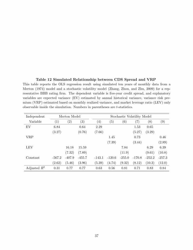
Table 12 Simulated Relationship between CDS Spread and VRPThis table reports the OLS regression result using simulated ten years of monthly data from a

Merton (1974) model and a stochastic volatility model (Zhang, Zhou, and Zhu, 2009) for a rep-

resentative BBB rating firm. The dependent variable is five-year credit spread, and explanatory

variables are expected variance (EV) estimated by annual historical variance, variance risk pre-

mium (VRP) estimated based on monthly realized variance, and market leverage ratio (LEV) only

observable inside the simulation. Numbers in parentheses are t-statistics.

Independent Merton Model Stochastic Volatility Model

Variable (1) (2) (3) (4) (5) (6) (7) (8) (9)

EV 6.84 0.64 2.29 1.53 0.65

(3.27) (0.76) (7.66) (5.27) (3.29)

VRP 1.45 0.73 0.46

(7.39) (3.44) (2.89)

LEV 16.18 15.59 7.84 6.29 6.39

(7.32) (7.89) (11.9) (9.61) (10.8)

Constant -567.2 -407.9 -455.7 -143.1 -120.6 -255.0 -170.8 -252.2 -257.3

(2.62) (5.46) (3.96) (5.39) (4.74) (9.32) (8.12) (10.3) (12.0)

Adjusted R2 0.31 0.77 0.77 0.63 0.56 0.81 0.71 0.83 0.84

37

Fig

ure

1T

he

tim

ese

ries

of

the

five-y

ear

CD

Ssp

reads

Th

isfi

gure

plo

tsth

efi

ve-y

ear

CD

Ssp

read

sof

full

sam

ple

and

thre

esu

b-s

amp

les.

We

grou

pth

eC

DS

spre

ad

sin

toth

ree

sub

-sam

ple

sby

CD

Sra

tin

gs.

Th

efi

rst

grou

pco

nta

ins

CD

Sof

AA

A,

AA

and

Agr

ades

.T

he

seco

nd

grou

pco

nta

ins

CD

Sof

BB

Bgra

de.

Th

eth

ird

gro

up

conta

ins

CD

Sof

spec

ula

tive

grad

esra

ngi

ng

bet

wee

nB

Ban

dC

CC

.T

he

thre

esu

b-s

amp

les

conta

in7,

315,

9,5

82

an

d5,1

07

ob

serv

ati

on

s

resp

ecti

vely

.T

he

CD

Ssp

read

sd

ecre

ase

grad

ual

lyfr

omth

ep

eaks

inla

te20

02,

then

incr

ease

agai

nas

the

fin

an

cial

cris

isap

pro

ach

esin

year

2007

.T

he

spre

ads

ofin

vest

men

tgr

ade

CD

Sin

year

2008

are

hig

her

than

thos

ein

year

2002

,w

her

eas

the

spre

ad

sof

spec

ula

tive

grad

eC

DS

are

low

erth

anth

eir

2002

leve

l.T

hat

hig

hli

ghts

the

nat

ure

ofth

ere

cent

fin

anci

alcr

isis

wh

ich

was

fuel

edm

ost

lyby

the

fin

anci

ald

istr

ess

ofh

igh

lyra

ted

cred

itp

rod

uct

s.T

he

diff

eren

ceb

etw

een

the

CD

Ssp

read

sfo

rin

vest

men

tgra

de

an

dsp

ecu

lati

vegro

up

CD

Sh

owev

erb

ecom

esw

iden

pot

enti

ally

due

toth

e”fl

y-t

o-qu

alit

y”

effec

td

uri

ng

the

fin

anci

alcr

isis

,d

rivin

gu

pco

mp

ensa

tion

for

cred

it

risk

.

0200400600Basis points

2001

2002

2003

2004

2005

2006

2007

2008

Tim

e

All

AA

A~A

BB

BB

B~C

CC

38

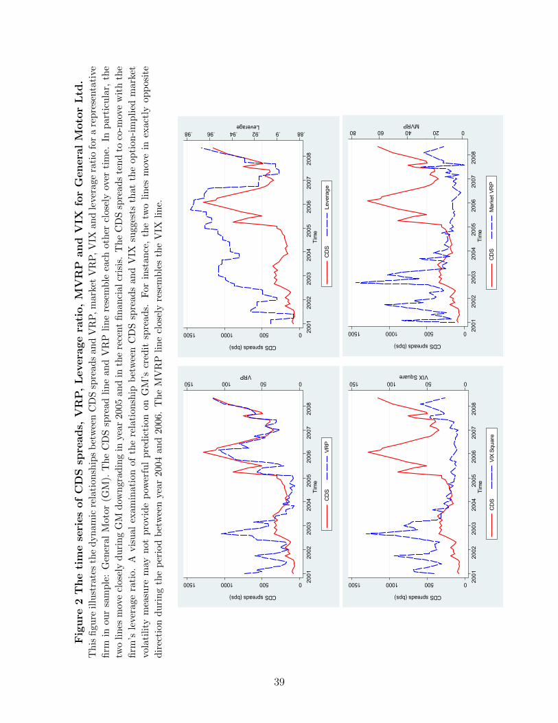
Fig

ure

2T

he

tim

ese

ries

of

CD

Ssp

reads,

VR

P,

Levera

ge

rati

o,

MV

RP

and

VIX

for

Gen

era

lM

oto

rL

td.

Th

isfi

gure

illu

stra

tes

the

dyn

amic

rela

tion

ship

sb

etw

een

CD

Ssp

read

san

dV

RP

,m

arket

VR

P,V

IXan

dle

vera

ge

rati

ofo

ra

rep

rese

nta

tive

firm

inou

rsa

mp

le:

Gen

eral

Mot

or(G

M).

The

CD

Ssp

read

lin

ean

dV

RP

lin

ere

sem

ble

each

oth

ercl

ose

lyov

erti

me.

Inp

art

icu

lar,

the

two

lin

esm

ove

clos

ely

duri

ng

GM

dow

ngr

adin

gin

year

2005

and

inth

ere

cent

fin

anci

alcr

isis

.T

he

CD

Ssp

read

ste

nd

toco

-mov

ew

ith

the

firm

’sle

vera

gera

tio.

Avis

ual

exam

inat

ion

ofth

ere

lati

onsh

ipb

etw

een

CD

Ssp

read

san

dV

IXsu

gges

tsth

at

the

op

tion

-im

pli

edm

ark

et

vola

tili

tym

easu

rem

ayn

otp

rovid

ep

ower

ful

pre

dic

tion

onG

M’s

cred

itsp

read

s.F

orin

stan

ce,

the

two

lines

mov

ein

exact

lyop

posi

te

dir

ecti

ond

uri

ng

the

per

iod

bet

wee

nye

ar20

04an

d20

06.

Th

eM

VR

Pli

ne

clos

ely

rese

mb

les

the

VIX

lin

e.

050100150VRP

050010001500

CDS spreads (bps)

2001

2002

2003

2004

2005

2006

2007

2008

Tim

e

CD

SVR

P

.88.9.92.94.96.98Leverage

050010001500

CDS spreads (bps)

2001

2002

2003

2004

2005

2006

2007

2008

Tim

e

CD

SLe

vera

ge

050100150VIX Square

050010001500

CDS spreads (bps)

2001

2002

2003

2004

2005

2006

2007

2008

Tim

e

CD

SVI

X Sq

uare

020406080MVRP

050010001500

CDS spreads (bps)

2001

2002

2003

2004

2005

2006

2007

2008

Tim

e

CD

SM

arke

t VR

P

39

Fig

ure

3F

itte

dV

RP

s/E

quit

yR

etu

rns

vers

us

obse

rved

VR

Ps/

Equit

yR

etu

rns

Th

isfi

gure

plo

tsfi

tted

VR

Ps

(equ

ity

retu

rns)

vers

us

obse

rved

VR

Ps

(equ

ity

retu

rns)

.T

he

fitt

edV

RP

(equ

ity

retu

rn)

for

firm

iis

esti

mat

edasVRPi

=λ̂VRP

0+λ̂VRP

1×β̂VRPi

(Ri

=λ̂CAPM

0+λ̂CAPM

1×β̂CAPMi)

,w

her

eth

eλ′ s

andβ′ s

are

esti

mate

du

sin

gth

est

an

dard

two-

stag

ere

gres

sion

sof

test

ing

CA

PM

.In

the

firs

tst

age,

tim

e-se

ries

regr

essi

ons

for

each

firm

ito

esti

mate

itsβVRP

ian

dβCAPM

i,

resp

ecti

vely

:VRPit

=αVRP

i+βVRP

i×VRPMKT

t+ε it

for

VR

Pan

dRit

=αCAPM

i+βCAPM

i×RMKT

t+ε it

for

CA

PM

.T

hen

each

firm

’sav

erag

eV

RP

,VRPi,

and

aver

age

equ

ity

retu

rn,Ri,

are

com

pu

ted

resp

ecti

vely

.T

he

seco

nd

-sta

ge

cross

-sec

tion

al

regre

ssio

ns

are

VRPi

=λVRP

0+λVRP

1×β̂VRPi+ε i

for

VR

Pan

dRi

=λCAPM

0+λCAPM

1×β̂CAPMi+ε i

for

CA

PM

050100150Fitted VRP

050

100

150

Obs

erve

d V

RP

Adj

uste

d R

-squ

are

= 1

4.05

%

-5051015Fitted Equity Return

-50

510

15O

bser

ved

Equ

ity R

etur

n

Adj

uste

d R

-squ

are

= 0

.00%

40