van der Waals and Casimir Forces

Carsten HenkelInstitut fur Physik und Astronomie, Universitat Potsdam

preliminary lecture notes

Winter semester 2015/16

Contents

1 Introduction and History 31.1 Van der Waals gas . . . . . . . . . . . . . . . . . . . . . . . . . . . . 31.2 Van der Waals forces . . . . . . . . . . . . . . . . . . . . . . . . . . 41.3 Connection to intermolecular forces . . . . . . . . . . . . . . . . . . 51.4 Contemporary Applications . . . . . . . . . . . . . . . . . . . . . . . 6

2 Adhesion and Surface Forces 72.1 Macroscopic van der Waals forces . . . . . . . . . . . . . . . . . . . 7

2.1.1 Hamaker approximation . . . . . . . . . . . . . . . . . . . . 72.1.2 Surface forces . . . . . . . . . . . . . . . . . . . . . . . . . . 8

3 Forces between Fluctuating Dipoles 103.1 Overview . . . . . . . . . . . . . . . . . . . . . . . . . . . . . . . . 103.2 Keesom forces, permanent dipoles . . . . . . . . . . . . . . . . . . . 113.3 Debye forces . . . . . . . . . . . . . . . . . . . . . . . . . . . . . . 133.4 London & Eisenschitz 1930 . . . . . . . . . . . . . . . . . . . . . . . 14

3.4.1 Theory . . . . . . . . . . . . . . . . . . . . . . . . . . . . . 143.4.2 Experiments . . . . . . . . . . . . . . . . . . . . . . . . . . 18

3.5 Casimir & Polder 1948 . . . . . . . . . . . . . . . . . . . . . . . . . 18

4 Quantum Electrodynamics at a Surface 224.1 Lecture 07 Jan 2016 . . . . . . . . . . . . . . . . . . . . . . . . . . . 224.2 Spontaneous emission near a surface . . . . . . . . . . . . . . . . . . 24

5 Macroscopic forces from nothing: Casimir effect 255.1 Casimir interaction between two mirrors . . . . . . . . . . . . . . . . 25

5.1.1 Sketch of derivation . . . . . . . . . . . . . . . . . . . . . . 255.1.2 Sum minus integral . . . . . . . . . . . . . . . . . . . . . . . 27

5.2 Failure of Heuristics . . . . . . . . . . . . . . . . . . . . . . . . . . 295.3 Lifshitz formula . . . . . . . . . . . . . . . . . . . . . . . . . . . . . 30

1

Ubersicht

van der Waals-Wechselwirkung: historischer Abriss. Adhasion, Oberflachen-Spannung, einfache Korper, Kolloide. London-Theorie: fluktuierende Dipole, klas-sisch und quantenmechanisch. Casimir-Polder-Theorie und virtuelle Photonen. Lamb-Verschiebung, spontaner Zerfall und Spektroskopie an Oberflachen. Lifshitz-Theorieund Rytov-Formulierung der Elektrodynamik. Messung von Casimir-Kraften undTests der Quantenfeldtheorie (Gravitation, funfte Kraft). Kritische Casimir-Energiein Flussigkeiten.

2

Chapter 1

Introduction and History

Johannes Diderik van der Waals (1837–1923). Nobel prize 1910 for his work on theequation of state of gases and liquids. First teacher in Leiden, Deventer, and Den Haag,and part-time student in physics and mathematics in Leiden (no Abitur). Finished 1873his PhD in physics (Leiden). Professor at Amsterdam University from 1877 to 1908.

Wikipedia (german): “discovered 1869 the origin of the attractive forces betweenatoms and non-polar molecules”. In his PhD (1873), he developed the van der Waalsequation of state for gases and liquids, showing that both phases and their phase tran-sition can be understood from the same physical principles.

1.1 Van der Waals gas

Equation of state

p =kTN

V − bN − aN2

V 2(1.1)

with pressure p, absolute temperature T , Boltzmann constant k = kB, volume V andparticle number N . (Different forms with number of moles and gas constant R arepossible.)

Two additional parameters a, b compared to the ideal gas

ideal gas: p =kTN

V(1.2)

have the interpretation:

• ‘excluded volume’ b (per particle): N particles occupy a ‘proper volume’ bN sothat the available volume is reduced, V 7→ V − bN . This increases the pressurecompared to an ideal gas with the same N , V ;

3

• coefficient a of ‘cohesion (internal) pressure’: the particles attract each otherso that at the surfaces of the container, they are pulled into the bulk of the gas,reducing the pressure. This arises from attractive ‘two-body interactions’, there-fore the change in pressure is negative and proportional to the square of thedensity p 7→ p− a(N/V )2.

(Different comparisons between the van der Waals and the ideal gas are possibledepending on what parameters are kept constant.)

In honor of his postulate that gas particles attract each other, intermolecular forcesare called Van der Waals forces. (Recall that around 1870, the existence of atoms andmolecules was not yet broadly accepted.)

3 Isothermen des p-V-Diagramms

⇔ p(V ) =nRT

V − nb− a

! n

V

"2

1/V 2

G

dG = 0

⇔ −SdT + V dp = 0

⇒ V dp = 0, dT = 0

⇔ p = konst.

Maxwell-Konstruktion

4 Abschätzung der kritischenGrößen

dp

dV=

d2p

dV 2= 0

•

⇒ Tc =8a

27bR

•

pc =a

27b2

•

Vm,c = 3b

•

Figure 0.1: Isothermal pressure p vs volume V in a van der Waals gas. Red line:critical temperature. Dark blue lines with horizontal parts (Maxwell construction):liquid phase. Light blue lines: gas phase. Credits: wikipedia.

The van der Waals equation of state predicts a phase transition between a gas anda liquid: this happens when in a pV -diagram (figure) the isothermal lines have anintermediate maximum.

1.2 Van der Waals forces

General name for weak forces between neutral particles (atoms, molecules). Can benaturally split into three types

4

• between permanent dipoles: Keesom force. These molecules have dipole mo-ments ‘rigidly attached’ to their molecular structure, for example water H2O andhydrochlorine HCl. In the gas phase, the molecules can rotate freely and becomecorrelated in their mutual orientation by electrostatic forces.

• between a permanent dipole and a polarizable molecule: Debye force. Here thefield generated by the dipole is polarizing a nearby molecule so that a dipolemoment is induced. This also leads to a correlation and an interaction betweenthe orientation of the dipole and the induced dipole.

• between polarizable molecules: London force or van der Waals force in the nar-row sense. Here, one has to invoke fluctuations in the dipole moments whosefields generate a correlation between the fluctuating dipoles. This leads, despitethe average over fluctuations, to a net interaction. These van der Waals forceswere the focus of the seminal paper by Eisenschitz & London (1930).

1.3 Connection to intermolecular forces

From statistical mechanics: virial expansion of the partition function, for small densi-ties where pair-, triple-, ... interactions become weaker and weaker. Leads to expansionfor the pressure in the form

p = nkT(1 +B2n+B3n

2 + . . .)

(1.3)

where the Bn are called the virial coefficients. They depend on the interactions be-tween n particles. In the grand-canonical ensemble of statistical mechanics, Bn canbe calculated from the partition function of a system with n particles (‘cluster expan-sion’).

Ideal gas: all B2 = B3 = . . . = 0

Van der Waals gas, approximately: keep only second virial coefficient B2. Link topair interaction energy W (ri, rj):

B2(T ) =1

2

∫d3r′ 1− exp[−W (r, r′)/kBT ] (1.4)

This does not depend on r when the interaction depends only on the distance, W =

W (r − r′) which is the typical behaviour in the bulk of a gas. One also assumes herethat the molecules have ‘no structure’: no information about the molecular orientationappears in W .

Exercise: show that for a hypothetical system with a repulsive van der Waals po-tential, W (r) = +c6/r

6, the virial coefficient is a simple root

B2(T ) = a

√c6

kBT(1.5)

5

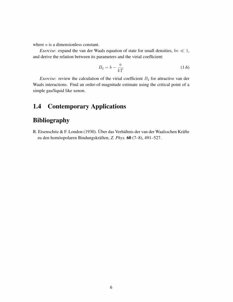
where a is a dimensionless constant.Exercise: expand the van der Waals equation of state for small densities, bn 1,

and derive the relation between its parameters and the virial coefficient:

B2 = b− a

kT(1.6)

Exercise: review the calculation of the virial coefficient B2 for attractive van derWaals interactions. Find an order-of-magnitude estimate using the critical point of asimple gas/liquid like xenon.

1.4 Contemporary Applications

Bibliography

R. Eisenschitz & F. London (1930). Uber das Verhaltnis der van der Waalsschen Kraftezu den homoopolaren Bindungskraften, Z. Phys. 60 (7–8), 491–527.

6

Chapter 2

Adhesion and Surface Forces

2.1 Macroscopic van der Waals forces

2.1.1 Hamaker approximation

Basic principle (and approximation): the interaction (energy) between two bodies isthe sum of all pair interactions. Hence if nA(r) and nB(r) are number densities ofmolecules in body A, B, we have

UAB =∫

Ad3r nA(r)

∫

Bd3r′ nB(r′)W (r, r′) (2.1)

H. C. Hamaker (1937) worked out some details between spherical particles in his clas-sic paper “The London-Van der Waals attraction between spherical particles,” [Physica4(10), 1058–72]. He introduced in particular the Hamaker constant

A = π2nAnBc6 (2.2)

for the van der Waals interactionW = −c6/r6. Typical numbers are in the microscopic

range A ∼ 0.1 . . . 1 eV and do not show a big variation across materials. We shall seelater in the lecture how this number comes about.

Exercise: when the constant A is factored out, the Hamaker interaction betweentwo bodies depends only on their shape, relative orientation, and ratio of length scales,but not on absolute distances. Details will follow.• The approximation behind Hamaker’s Ansatz neglects the fact that electric fields

are ‘screened’ by macroscopic bodies: they do not penetrate as easily as in free space.This is often forgotten, maybe because Eq.(2.1) is very natural when we are dealingwith the gravitational interactions – for which there is no screening.

On the other hand, in many applications, we are dealing with bodies in a fluid likewater – the forces between them are then modified because water is screening electric

7

fields. By adding a small amount of salt concentration, for example, one can inducebig changes.

More examples of different shapes are discussed in Langbein’s book “Theory ofVan der Waals attraction” and for example by R. Tadmor, “The London-van der Waalsinteraction energy between objects of various geometries,” J. Phys.: Condens. Matter13 (2001) L195–202.

2.1.2 Surface forces

Geometrical argument that for ‘large’ bodies with quasi-planar surfaces, the forcescales with the size of the ‘contact area’. For two plates, for example, one finds thatthe force per unit area is given by

F

area= −(· · ·)A

d3(2.3)

where A is the Hamaker constant and d the distance between the bodies. The minussign means that the force is attractive. Forces like this that scale with the area arecalled ‘surface forces’, and one speaks of a surface stress (force per area or pressure).The force law (2.3) is only valid down to distances d ∼ 0.4 . . . 1 nm where ‘chemistry’(hydrogen bonds, overlap of electron orbitals . . . ) comes into play.

For the estimation of Hamaker constants between different materials, there aremany resources on the web, for example the lecture by G. Ahmadi from ClarksonUniversity.

In many applications, bodies are not smooth, and the actual contact area is muchsmaller because only ‘mountains’ or ‘protuberances’ touch, while distances between‘valleys’ are much larger. One may loosely define the contact area as those pointswhere the distance is of the order 1 nm. Adhesion through surface forces can becomestrong up to the point that they can carry the weight of a body. This happens when thecontact area increases, for example by giving one body a flexible shape or by usingsmooth contact surfaces. In glues, one uses a fluid to smoothen the surfaces. Insectsand animals like geckos use this surface force to climb glass and other walls.

The surface force plays an important role in continuum mechanics and competeswith ‘deformation stress’ when two bodies touch. For a contemporary example, seethe guest lecture by F. Spahn.

Bibliography

H. C. Hamaker (1937). The London–van der Waals attraction between spherical parti-cles, Physica 4 (10), 1058–72.

8

D. Langbein (1974). Theory of Van der Waals attraction, volume 72 of Springer Tractsin Modern Physics. Springer, Berlin.

R. Tadmor (2001). The London-van der Waals interaction energy between objects ofvarious geometries, J. Phys.: Condens. Matter 13 (9), L195–202.

9

Chapter 3

Forces between Fluctuating Dipoles

3.1 Overview

See Sec.1.2: Keesom forces between permanent dipoles, Debye forces between a per-manent dipole and a polarizable particle, London–van der Waals forces between twopolarizable particles.

The permanent dipoles can be treated, in the simplest approximation, with classi-cal statistical mechanics. See also in Jackson’s book the section on ‘Models for theMolecular Polarizability’.

Water: d = 1.85 D with the Debye 1 D = 0.39343 ea0 a conventional unit formolecular dipole moments.

free (Gibbs) energy, more precisely free energy of interaction and partition functionZ (Zustandssumme)

Z =∫d(· · ·) e−E(···)/kT = e−G/kT (3.1)

where (· · ·) is symbolic for the parameters of the possible states of the system. Thisfree energy is a thermodynamic potential and determines for example the force be-tween two particles

F = −∇RG R : particle coordinate (3.2)

One says that F is ‘conjugate’ to R. But the same formula also applies when R is an-other parameter like the volume of the system (the derivative then gives the pressure).The thermodynamic entropy of the system is conjugate to the temperature itself:

S = −∂G∂T

(3.3)

It gives the ‘entropy of interaction’, related to the ‘amount of disorder’ subject to theconstraint of fixed positions of a particle, for example. In some applications, one also

10

speaks of ‘entropic forces’ – they arise not from a change in (potential) energy, but indisorder.

The inner energy U is the average of E(· · ·) over the Boltzmann distribution ofstates, and given by

U = G+ ST = −kT logZ (3.4)

3.2 Keesom forces, permanent dipoles

Close to problem from school on Casimir physics (Leiden 2012).We take the two dipole moments as having a fixed length (the same for simplicity),

dA = da , dB = db (3.5)

so that the summation over all states is the integral over two unit spheres (a cartesianproduct of two spheres) with solid angle element dΩ(a) dΩ(b).

The energy of the two dipoles is given by electrostatics

E(a, b) = −dA · E(rA|B) =dA · dB − 3(r · dA)(r · dB)

4πε0|rA − rB|3(3.6)

where r is the unit vector along the distance vector rA− rB. In the following, we writer = |rA − rB| and use the tensor

dA · dB − 3(r · dA)(r · dB) = dA · gdBg = 1− 3r r· (3.7)

This is a linear map of vectors into vectors. The notation r r· means: take the scalarproduct with the vector you act upon and multiply the result with r. One also findsoften the notation r⊗ r which means the same.

Check the exponent: potential between two charges has 1/r (Coulomb law). Forthe dipole, put two opposite charge closely together, so this gives a 1/r2 potential.Take the derivative for the electric field.

Simple limiting cases to check the signs: dipoles ‘head to tail’ attract each other =d and r are parallel, and the energy is negative (lowest energy at close distance). Sign+1 − 3 = −2. Dipoles ‘parallel and side by side’ repel = d and r are perpendicular,potential is positive. Sign +1.

Typical scale. Boltzmann factor involves the dimensionless ratio

E(a, b)

kT=

d2

4πε0 r3kT

(a · b− 3(r · a)(r · b)

)= u(a · g b) (3.8)

11

Typical value for parameter u: d = 1.85 D (water), T = 300 K,

u ≈ 0.08 nm3

r3(3.9)

hence for distances above r = 1 nm, this is small: the Keesom interaction is weakcompared to the thermal energy. We are going to expand the Boltzmann factor.

See exercises from Leiden 2012 for a calculation with spherical coordinatesθA, ϕA, θB, ϕB. Integrals in partitional function are tedious, but relatively straight-forward.

Here a simpler way: keep components of the dipole vectors.The Taylor expansion can be integrated term by term:

Z =∫

dΩ(a)dΩ(b)(1− u(a · g b) +

u2

2(a · g b)2 + . . .

)(3.10)

The first term, 1, does not diverge because the ‘state space’ is finite (the unit spherehas finite area). It gives Z0 = (4π)2.

The second term can be factorized into integrals∫

dΩ(a) a = 0 (3.11)

for ‘symmetry reasons’: we sum over all directions, and for each one, with the sameweight appears the opposite one.

The third term is quadratic in a and b and does not vanish. We write out the squareinto a sum over components (Einstein summation convention)

(a · g b)2 = aigijbjakgklbl (3.12)

where gij is the matrix representation of the tensor g.Again for symmetry reasons, we can argue∫

dΩ(a) aiak = δik

∫dΩ(a) a2

i =δik3

∫dΩ(a)(a2

x + a2y + a2

z) = δik4π

3(3.13)

The four sums in Eq.(3.12) reduce eventually to (summation convention!)∫

dΩ(a)dΩ(b)aigijbjakgklbl =(4π

3

)2δikgijδjlgkl =

(4π

3

)2gilgil =

(4π

3

)2trgT g

(3.14)where gT is the transposed tensor and tr is the trace (sum over diagonal elements). Inthe tensor notation (3.7), this is easy to work out: g is symmetric and1

gT g = g g = 1+ 3r r· (3.15)1For a general tensor product uv·, we have (uv·)T = vu· by definition. Its matrix elements are

(uv·)ik = uivk.

12

the trace of which is . . . 6. (See footnote 1 on page 12 and remember that r is a unitvector.)

The partition function (3.10) is therefore, up to order u2:

Z = Z0

(1 +

u2

3

)(3.16)

Taking the logarithm, dropping the first constant and expanding for small u, we get thefree Gibbs energy for the Keesom interaction

Keesom : G = −kT u2

3= − d4

3(4πε0)2kT

1

r6= −c6

r6(3.17)

This is our first calculation of a van der Waals force constant c6.

3.3 Debye forces

Energy between dipole A and polarizable particle B

E = −αB2E2(rB|A) (3.18)

with polarizability giving the induced dipole moment dB = αBE(rB). The factor 1/2

arises because this is the potential energy of an induced dipole.Same thermodynamic calculation (just take the average over the orientation of

dipole A, no further variables for particle B) gives a free energy

Debye : G = − d2AαB

3(4πε0)2

1

r6(3.19)

which is also a 1/r6 law, but with a different temperature dependence. A typical num-ber is for the Rb atom (in the alkali series) αB/(4πε0) ≈ 47 A

3.

Comparison The Debye interaction does not depend on temperature. Its entropy iszero. For the Keesom interaction, one gets an inner energy twice as large as the freeenergy, the entropy increases with lower temperature. If the free energy were linear inT , we would have a purely entropic interaction, U = 0.

Keesom Debyefree energy G ∼ 1/T G ∼ const.

Entropy S ∼ −1/T 2 S = 0

inner energy U = 2G U = G

13

3.4 London & Eisenschitz 1930

non-retarded (electrostatic) case Eisenschitz & London (1930); London (1930)including retardation Casimir & Polder (1948)

3.4.1 Theory

Two atoms

Basic idea: second-order perturbation theory using the electrostatic interaction be-tween dipole moments

V =dA · dB − 3(r · dA)(r · dB)

4πε0|rA − rB|3(3.20)

which is the same as Eq.(3.6), except that dA,B are now quantum-mechanical opera-tors.

Overview on states in Hilbert space that are coupled by this interaction:

• selection rules for dipole operator (‘skew’): connects different states / energylevels

• ground state |gg′〉 = |g〉A ⊗ |g′〉B and doubly excited states |ee′〉 (no couplingfrom ground state to |eg′〉)

• second-order perturbation theory → van der Waals energy shift of the groundstate atom pair

W = −∑

e,e′

|〈ee′|V |gg′〉|2Ee + Ee′ − Eg − Eg′

(3.21)

where the ‘energy mismatch’ is the sum of two Bohr frequencies

Ee + Ee′ − Eg − Eg′ = h(ωeg + ωe′g′) (3.22)

Matrix elements factorize (summation convention and using the electrostatic tensor gfrom Eq.(3.7))

〈ee′|V |gg′〉 = 〈e|di|g〉gij

4πε0r3〈e′|dj|g′〉 (3.23)

We see immediately that the leading-order shift from Eq.(3.21) scales like 1/r6. Inaddition, the interaction is attractive because in the sum in Eq.(3.21), all terms havethe same sign. This is a typical result for the perturbation theory in the ground state.

14

Challenge: need many spectroscopic informations about energy levels and dipolematrix elements. Idea of Eisenschitz & London (1930): provide a connection to an-other quantity that can be directly measured. With the approximation that ‘all relevantBohr frequencies’ are roughly the same, one gets for example

1

Ee + Ee′ − Eg − Eg′≈ 1

h(ωA + ωB)(3.24)

which is approximated further to generate a product of properties of atom A and atomB. In the modern formulation, one uses the ‘factorization trick’

1

h(ωeg + ωe′g′)=

2

πh

∞∫

0

dξωeg

ω2eg + ξ2

ωe′g′

ω2e′g′ + ξ2

(3.25)

it turns out that the summation over the excited states can be expressed in terms ofthe polarizabilities. These are frequency-dependent tensors αij(ω) that provide, as inclassical electrodynamics, the dipole moment induced by a weak, oscillating electricfield (in the stationary limit)

〈di(t)〉 = αij(ω)Ej e−iωt + c.c. (3.26)

The additional feature in quantum mechanics is that this dipole moment is the (per-turbed) average of an operator. (The field is described classically with a complexamplitude Ej at the position of the atom.) As in classical linear response theory, thepolarizability is a complex function; its imaginary part shows narrow peaks at the ab-sorption lines of the atom, hω ≈ Ee − Eg. Note that αij(ω) is also specific for thestate that the atom starts in (here: the ground state). From time-dependent perturbationtheory, one finds that (see exercises)

αij(ω) =∑

e

2ωeg〈g|di|e〉〈e|dj|g〉ω2eg − (ω + i0)2

(3.27)

where the ‘+i0’ is a prescription related to causality that makes αij(ω) a analytic func-tion in the upper half-plane of complex frequencies.

Indeed, the van der Waals interaction can be written as an integral over polarizabil-ities along the upper imaginary axis (see exercises for details)

W (r) = − h

(4πε0)2r6

∞∫

0

dξ

2παki(iξ)gijα

′lj(iξ)g

∗kl (3.28)

Note that the polarizabilities αki(iξ) are positive under the integral so that the sign ofthe van der Waals interaction is ‘stable’.

15

Figure 0.1: Qualitative behaviour of polarizability α for real and imaginary fre-quencies.

Let us make the assumption that the polarizabilities are isotropic, αij = δijα (at-tention, other conventions introduce a factor 1/3 here). This happens when the groundstate is spherically symmetric (an s-state, for example). This is also typical for thenoble gas atoms Eisenschitz & London (1930) focused on anyway. The summationover the indices then brings us back to the trace of Eq.(3.14), and we can read off theformula for the c6-coefficient:

W (r) = −c6

r6, c6 =

6h

(4πε0)2

∞∫

0

dξ

2πα(iξ)α′(iξ) (3.29)

This integral is computed out today with high precision in atomic and molecularphysics, using much more accurate models for the electronic structure.

A simple ‘two-level model’ takes only one excited state in the polarizabilityEq.(3.27). We can also use the fact that α(iξ) is nonzero up to a typical Bohr frequency(or ionization energy) and decays in the UV. The c6-integral can then be estimated as

c6 '6hωAB(4πε0)2

αAαB (3.30)

where the αA,B are now the static polarizabilities and hωAB an averaged ionizationenergy.

Atom+surface potential

Simple Hamaker scheme: integrate over atoms of the surface. Gives∫

z′<0

dV ′n′

|r− r′|6 =πn′

6z3(3.31)

where n′ is the number density of the surface and z the distance between atom andsurface. The van der Waals potential is then proportional to n′α′ which is only true fora ‘dilute body’.

16

Figure 0.2: Atomic dipole and its images in a perfectly reflecting surface. This is amodel that reproduces the actual charge distribution on the conducting surface andthe electric field lines outside.

Opposite limit: consider the surface as a perfect reflector and re-start from electro-statics – the atom interacts with its image dipole

image interaction V =1

2

d′ · d− 3(z · d′)(z · d)

4πε0(2z)3(3.32)

Here, d′ is the image dipole: parallel to d if d is perpendicular to the surface, andanti-parallel if d is normal to it. (This behavior is explained by the image of a charge,where one has to change the sign of the charge.) The factor 1/2 arises because theimage dipole is induced by the dipole itself. In a similar tensor formulation as before

d′ = −(1− 2zz·)d = md (3.33)

and the interaction (3.32) becomes

V =(md) · gd8πε0(2z)3

=d ·mTgd

8πε0(2z)3= −d2 + (z · d)2

8πε0(2z)3(3.34)

where the expression g = 1− 3zz· for the electrostatic tensor between the dipole andits image (‘directly below in the surface’) was used.

Now the quantum mechanics goes as before. Here, we are even done with first-order perturbation theory and W = 〈g|V |g〉. We observe that the interaction is attrac-tive and anisotropic: it is twice as strong for atoms with dipole moments perpendicularto the surface. But for the typical case of an isotropic atom, the expectation value ofthe ‘dipole fluctuations’ is

〈g|didj|g〉 =1

3〈g|d2|g〉δij (3.35)

(note the factor of 1/3 which is not conventional). We then get in Eq.(3.34) a term43〈g|d2|g〉 from the anisotropic dipole fluctuations, and the atom-surface van der Waals

potential becomes

W (z) = −〈g|d2|g〉

48πε0 z3(3.36)

Two-level model: approximate 〈g|d2|g〉 ≈ |〈e|d|g〉|2 and express this by the sponta-neous decay rate

γe =|〈e|d|g〉|2ω3

eg

3πε0hc3(3.37)

With the wavenumber keg = ωeg/c, we then get the convenient parametrization

W (z) ≈ − hγe16(kegz)3

(3.38)

17

The error of this approximation can be up to 25% because of other levels (includingthe continuum) that contribute to the dipole fluctuations 〈g|d2|g〉.

Refinement: dielectric surface with frequency-dependent surface charge. This canbe expressed by a dielectric function ε(ω) for the material in the surface. The imagedipole then gets the additional factor

dielectric image d′ =ε(ω)− ε0

ε(ω) + ε0

md (3.39)

as is known from electrostatics. We recover the perfect conductor in the formal limitε(ω)→∞. But the ‘dilute limit’ can also be taken by using the dielectric function ofa gas of atoms, ε(ω) ≈ ε0 + nα(ω) where α(ω) is the polarizability per atom and nthe number density.

The evaluation of the second-order perturbation theory then leads to the integral(Wylie & Sipe, 1984)

W (z) = − h

8πε0 z3

∞∫

0

dξ

2π

ε(iξ)− ε0

ε(iξ) + ε0

α(iξ) (3.40)

We emphasize that this is valid as long as electrostatic images can be used (non-retarded distances) and as long as the surface can be described macroscopically (localdielectric function, i.e., distances large compared to the atomic scale).

Exercise: check that the dilute limit (dielectric function of a gas) gives back thenaive Hamaker result. Check that the perfector conductor limit gives the result fromimage dipoles.

3.4.2 Experiments

atom–surface physisorption potential (Pollard, 1941; McLachlan, 1964)atom–surface scattering Beeby (1971); Beeby & Thomas (1974)atomic beam deflection Sandoghdar & al. (1992); Sukenik & al. (1993)cold atom reflection Landragin & al. (1996); Bender & al. (2010)

3.5 Casimir & Polder 1948

Re-calculation of the atom-atom van der Waals interaction, using a slightly differentquantum-mechanical description:

• degrees of freedom: dipole moment of atom A and atom B

• and electromagnetic field = infinite set of field modes, each treated as a harmonicoscillator

18

Eur. Phys. J. D (2012) 66: 321 Page 7 of 11

0.1 1 10 100 1000!2

!1.5

!1

!0.5

0

CC

CL

dielectric

λA λT

semiconductor

distance z [a0]

c 3co

effici

ent

[α(0

)kBT

]

Fig. 3. (Color online) Atom-surface potential through theCasimir-Polder range up to the thermal wavelength. We plotthe c3 coefficient of the free energy, i.e. F(z)z3, but here inunits of α(0)kBT . The distance is normalized to the screen-ing length a0 ≈ 73 nm. Solid thick curve: local dielectric func-tion in Drude form; dashed curve: charge layer (CL) model;dotted curve: hydrodynamic (continuous charge, CC) model;solid thin curve: non-conducting local dielectric. Parameters:background dielectric constant ϵ∞ = 1.5, DC conductivityσ = 1010 s−1 (comparable to Ge), electron scattering time τ =τs = 10−13 s, diffusion constants D = Ds = 4.5 cm2/s, atomicresonance Ω/2π = 477 THz (wavelength 2πλA = 628 nm),Temperature T = 300 K (thermal wavelength λT = 7.6 µm).

In Figure 3, we show the free energy of interaction F(z)calculated from the Matsubara sum (9). At distances be-yond the thermal wavelength λT , the free energy followsa 1/z3 power law with a c3 coefficient proportional to Tthat we discuss in the following section. The differencebetween dielectric and Drude conductor arises, for theseparameters, from the zeroth term in the Matsubara sum.This term is discussed in more detail in Section 5. In-deed, in the other terms, the conductivity enters onlyin the ratio 4πσ/ξl = 2!σ/(lkBT ). At room tempera-ture, this ratio can be neglected compared to the back-ground dielectric constant ϵ∞ provided the conductiv-ity σ ≪ 4 × 1013 s−1. This regime applies to a wide rangeof doped semi-conductors.

The van der Waals regime for this material is notdescribed by equation (20) due to the low conductiv-ity. Ignoring conductivity completely, equation (19) fora local dielectric gives a short-range coefficient c3 with avalue −1.91 α(0)kBT in the units of Figure 3: this corre-sponds well to the full calculation. We have checked thatthe small difference is actually due to relatively large devi-ations from the non-retarded approximation that was ap-plied to derive equation (19). A similar situation occurredin reference [39] which discusses the Casimir force betweentwo plates separated by a dielectric liquid.

5 Lifshitz (thermal) regime

This section deals with the long distance regime λT ≪ zwhere the leading contribution to the atom-surface po-tential is given by the l = 0 term in the Matsubarasum (9). The other terms are proportional to the exponen-tially small factor exp(−4πlz/λT ) and can be neglected if

the l = 0 term is nonzero. A glance at Figure 3 illus-trates that the thermal regime is already well borne outat z ∼ λT due to the factor 4π in the exponential.

The static term in the Matsubara sum has been thesubject of much discussion in the field of dispersion in-teractions [40,41]. To illustrate this, we give the limitingforms of the free energy in the thermal range for an idealdielectric material

λT ≪ z : F(z) ≈ −α(0)kBT

4z3

ϵ∞ − 1

ϵ∞ + 1, (30)

while for a conductor in the same limit

F(z) ≈ −α(0)kBT

4z3. (31)

In fact, the latter result is obtained for any material witha nonzero conductivity: as σ → 0, the former (dielec-tric) result is not obtained in a continuous manner [4].This is due to the static reflection coefficient rTM(0, k)which is equal to 1 for any nonzero σ, while setting σ = 0from the start for a pure dielectric, one gets rTM(0, k) =(ϵ∞ − 1)/(ϵ∞ + 1). This difference between conductorand dielectric is also visible in the Casimir-Polder rangeshown in Figure 3. The discontinuity disappears only inthe limit T = 0 for the material parameters consideredhere.

This effect is actually an artefact of the description interms of a local material response (conductivity, dielectricfunction). Using a hydrodynamic model similar to our CC,Pitaevskii has shown that the free energy shows a contin-uous cross-over between the limiting cases equations (30)and (31). We show now that the same is true for both CCand CL models considered here.

For the CC model, the first line of equation (9) can bewritten in terms of a dimensionless integral (t = 2kz)

λT ≪ z :

F(z) ≈ −α(0)kBT

8z3

∞!

0

dt t2e−t ϵ∞"

t2 + (2z/a0)2 − t

ϵ∞"

t2 + (2z/a0)2 + t,

(32)

with the screening length a0 of equation (1). We recoverPitaevskii’s result [5] by calculating a0 from the diffu-sion coefficient D ≈ kBT τ/m∗ of a non-degenerate elec-tron gas. This leads to a−2

0 = 4πnℓB where n is the car-rier density in the conductor and ℓB the Bjerrum length(i.e., the distance where the Coulomb energy betweentwo electrons becomes comparable to the thermal en-ergy: e2/(ϵ∞ℓB) = kBT ). A glance at equation (32) tellsthat the dielectric and metallic values of the reflectioncoefficient are smoothly interpolated as the ratio (z/a0)

2

changes from zero to infinity. This is illustrated in Figure 4(dotted line) where the coefficient of the 1/z3 power lawis plotted vs z/a0.

Figure 0.3: Evaluation of the atom-surface interaction for a more complete ap-proach. Included are retardation, the effect of finite temperature and a more de-tailed model of the electromagnetic response of the surface. The interaction energyW (z) is then replaced by the Gibbs free energy G(z) [denoted F(z) in the cap-tion] and we plot for better visibility the product z3G(z). Taken from Eizner & al.(2012).

19

• basic interaction of electric dipole type

V = −dA · E(xA)− dB · E(xB)

where xA,B are the positions of the two atoms. These are handled as before by Eisen-schitz & London (1930) as classical, fixed parameters.

Result for the atom-atom interaction: at distances much larger than typical transi-tion frequencies of the atoms, the potential is weaker and follows a power law

r λAB : W (r) ' −c7

r7(3.41)

This was motivated for this updated theory: experimental data from colloid physics(Verweey & Overbeek, 1948) that indicate that at ‘large distances’ (roughly 50 nm andbeyond), the van der Waals interaction between two atoms gets weaker than the 1/r6

power law predicted from London theory.Heuristic explanation that is often used: the electric fields that go from atom A to

atom B are getting ‘out of phase’ due to retardation and the wide range of frequencies.The destructive interference weakens the mutual polarization of the particles.

From a theoretical viewpoint, the main contribution of Casimir and Polder wasto re-introduce into the theory the intrinsic fluctuations of the electromagnetic field.These are commonly called ‘vacuum fluctuations’ because they even persist in emptyspace (one meaning of ‘vacuum’) and at zero temperature (no photons, other meaningof ‘vacuum’).

Result for the atom-surface interaction including retardation

W (z) = −h∞∫

0

dξ

2πRij(iξ, z)αji(iξ) (3.42)

whereRij(iξ, z) is the so-called ‘reflection tensor’ that gives the electric field scatteredback from the surface. It depends on the distance z of the dipole source from thesurface and on an angular average of reflection coefficients (including ‘complex anglesof incidence’). One can understand it as the ‘response function of the surface’, byanalogy to the polarizability (the response function of the atom).

Bibliography

J. L. Beeby (1971). The scattering of helium atoms from surfaces, J. Phys. C: Solid St.Phys. 4, L359–362.

J. L. Beeby & E. G. Thomas (1974). The long-range potential in the scattering ofatoms from surfaces, J. Phys. C 7, 2157–64.

20

H. Bender, P. W. Courteille, C. Marzok, C. Zimmermann & S. Slama (2010). DirectMeasurement of intermediate-range Casimir-Polder potentials, Phys. Rev. Lett. 104,083201.

H. B. Casimir & D. Polder (1948). The influence of retardation on the London-van derWaals forces, Phys. Rev. 73, 360–72.

R. Eisenschitz & F. London (1930). Uber das Verhaltnis der van der Waalsschen Kraftezu den homoopolaren Bindungskraften, Z. Phys. 60 (7–8), 491–527.

E. Eizner, B. Horovitz & C. Henkel (2012). Van der Waals–Casimir–Polder interactionof an atom with a composite surface, Eur. Phys. J. D 66 (12), 321. Highlight ‘Maythe force be with the atomic probe’ at.

A. Landragin, J.-Y. Courtois, G. Labeyrie, N. Vansteenkiste, C. I. Westbrook & A.Aspect (1996). Measurement of the van der Waals force in an atomic mirror, Phys.Rev. Lett. 77, 1464.

F. London (1930). Zur Theorie und Systematik der Molekularkrafte, Z. Phys. 63 (3),245–79.

A. D. McLachlan (1964). Van der Waals forces between an atom and a surface, Mol.Phys. 7 (4), 381–88.

W. G. Pollard (1941). Exchange Forces Between Neutral Molecules and a Metal Sur-face, Phys. Rev. 60 (8), 578–85.

V. Sandoghdar, C. I. Sukenik, E. A. Hinds & S. Haroche (1992). Direct measurementof the van der Waals interaction between an atom and its images in a micron-sizedcavity, Phys. Rev. Lett. 68, 3432–3435.

C. I. Sukenik, M. G. Boshier, D. Cho, V. Sandoghdar & E. A. Hinds (1993). Measure-ment of the Casimir-Polder force, Phys. Rev. Lett. 70 (5), 560–63.

E. Verweey & J. Overbeek (1948). Theory of the Stability of Lyophobic Colloids.Elsevier Science Publishers, Amsterdam.

J. M. Wylie & J. E. Sipe (1984). Quantum electrodynamics near an interface, Phys.Rev. A 30 (3), 1185–93.

21

Chapter 4

Quantum Electrodynamics at aSurface

4.1 Lecture 07 Jan 2016

Typical scenario in hydrogen atom: ‘fine structure splitting’ between 2p1/2 and 2p3/2

that differ in total angular momentum (orbital + spin). This was predicted in 1928by the Dirac equation, the relativistic generalization of the Schrodinger equation. Butalso the levels 2s1/2 and 2p1/2 are split by ≈ 1000 MHz, the Lamb shift experimen-tally measured in the early 1940s. This was quantitatively explained by Hans Bethearound 1948. It provides the first example of a finite result coming from subtractingformally infinite quantities in quantum electrodynamics (problem of regularization andrenormalization).

Calculation from Qualitative Methods in Quantum Theory by A. B. Migdal.Idea 1: change in potential energy as an electron is displaced, expanded for small

displacement δ

δV = V (x + δ)− V (x) = δ · ∇V +δiδj2

∂2V

∂xi∂xj+ . . . (4.1)

For the Coulomb potential, the second derivative is related to the charge density, lo-calized in the nucleus. Average δV over the electron orbital |ψn(x)|2 of a state withquantum numbers n (typical quantum argument): this gives the density |ψn(0)|2 atthe position of the nucleus. And average over the displacement δ of the electron,modelled from the electric field due to vacuum fluctuations. This calculation looks(semi)classical.

Idea 2: treat the response of the electron to the electric vacuum field first like aclassical force and use a heuristical argument to get the zero-point fluctuations in the

22

Figure 0.1: Willis Lamb with the Dirac equation and the level scheme of hydrogenin the n = 2 manifold. From the obituary published in Nature 453 (12 June 2008)867.

state with zero photons. In Fourier space

δω =−e/m

ω(ωA + ω)Eω (4.2)

where ωA is a ‘typical resonance frequency of the atom’ (replace detailed level struc-ture by a harmonic oscillator). The averages 〈δω〉 = 0 and 〈δiωδjω〉 = 1

3δij〈δ2

ω〉. Thevacuum field has a variance such that per k-vector (and polarization state σ) in thequantization volume V , the electromagnetic energy density (half electric, half mag-netic) integrates to one half quantum:

V ε0|Ekσ|2 'hω

2(4.3)

Sum over polarizations and k-vectors, convert into integral and start discussion aboutcutoff ωc

δEn ∼ he2|ψn(0)|2ωc∫

0

dω

ωA + ω∼ log

mc2

hωA(4.4)

Heuristic argument why a cutoff at hωc ∼ mc2 is plausible: at photon energies compa-rable to the electron rest mass, the electron responds more weakly to the electric fieldbecause of the relativistic increase in mass. Modern quantitative calculations start froma fully relativistic description for the electron (Dirac equation). They also yield a pre-cise expression for the ‘Bethe logarithm’ that involves more than one Bohr frequencyin the atom (see, e.g., Jentschura & al. (2005)).

23

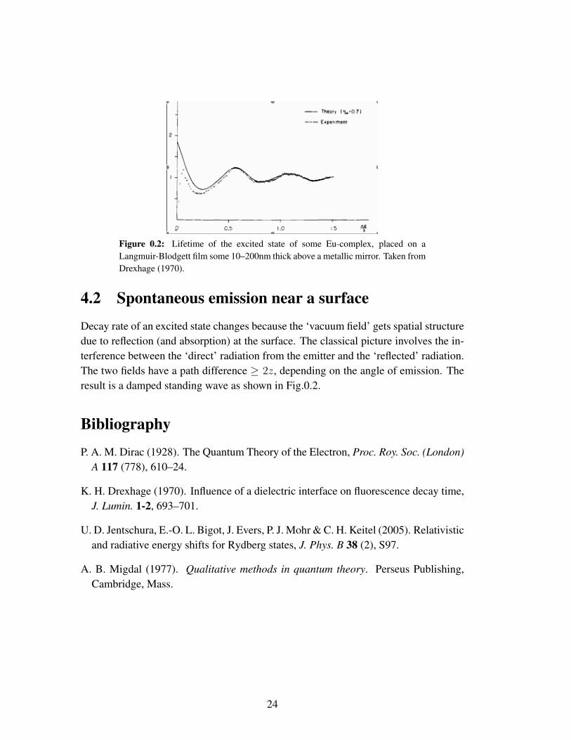
Figure 0.2: Lifetime of the excited state of some Eu-complex, placed on aLangmuir-Blodgett film some 10–200nm thick above a metallic mirror. Taken fromDrexhage (1970).

4.2 Spontaneous emission near a surface

Decay rate of an excited state changes because the ‘vacuum field’ gets spatial structuredue to reflection (and absorption) at the surface. The classical picture involves the in-terference between the ‘direct’ radiation from the emitter and the ‘reflected’ radiation.The two fields have a path difference ≥ 2z, depending on the angle of emission. Theresult is a damped standing wave as shown in Fig.0.2.

Bibliography

P. A. M. Dirac (1928). The Quantum Theory of the Electron, Proc. Roy. Soc. (London)A 117 (778), 610–24.

K. H. Drexhage (1970). Influence of a dielectric interface on fluorescence decay time,J. Lumin. 1-2, 693–701.

U. D. Jentschura, E.-O. L. Bigot, J. Evers, P. J. Mohr & C. H. Keitel (2005). Relativisticand radiative energy shifts for Rydberg states, J. Phys. B 38 (2), S97.

A. B. Migdal (1977). Qualitative methods in quantum theory. Perseus Publishing,Cambridge, Mass.

24

Chapter 5

Macroscopic forces from nothing:Casimir effect

5.1 Casimir interaction between two mirrors

Casimir (1948), elaborated upon suggestion by N. Bohr: ‘This (the Casimir-Poldershift) must have to do with vacuum fluctuations.’

The Casimir force is the attraction between two metallic mirrors placed in vacuum.It is interpreted in terms of the change in the zero-point energy (the famous 1

2hω of the

harmonic oscillator ground state) induced by the presence of the mirrors. We give herean sketch of the calculation done by Casimir around 1948. He found an energy (perarea) for two mirrors equal to

∆E

A= − π2

720

hc

L3(5.1)

so that the force per unit area (negative gradient) is FC/A = −π2hc/240L4: since theenergy decreases as L→ 0, the two mirrors placed in vacuum attract each other.

Note that this result is independent of the nature of the mirrors, as well as theirelectric charge. The electromagnetic field only enters inasmuch as its modes give acontribution to the energy of the vacuum state.

5.1.1 Sketch of derivation

We consider the ground state energy of the multi-mode electromagnetic field

E0 =∑

kλ

hωkλ

2

that is of course infinite and compare the cases of a planar cavity formed by two mirrors(distance L) and empty space (i.e., two mirrors infinitely apart). In the first case, we

25

have standing wave modes between the mirrors with a frequency

ω(cav) = c√K2 + k2

n, kn =nπ

L

with K2 = k2x + k2

y and n = 1, 2, . . ., while in empty space,

ω = c√K2 + k2

z

with −∞ < kz < ∞. We first compute the difference in the electromagnetic modedensity per volume AL where A is the ‘quantization area’ in the xy-plane. We cheatwith the polarizations and multiply by a factor 2:

ρL(ω) =4π

AL

∑

K,n

δ(ω − c

√K2 + k2

n

)

=2

L

∞∫

0

KdK∑

n

δ(ω − c

√K2 + k2

n

)(5.2)

The integration over K can be performed with the substitution K 7→ c√K2 + k2

n andgives

ρL(ω) =2ω

Lc2

∑

n

Θ(ω − ckn) (5.3)

where Θ is the step function. It arises because for a given n, there are no modes withfrequency smaller than ckn. The same calculation in the infinite volume gives

ρ∞(ω) =2ω

c2

∞∫

0

dkzπ

Θ(ω − ckz) (5.4)

The kz integral can of course be performed, but we keep it here to illustrate one ofthe basic features of the Casimir calculation: the result originates from the differencebetween a ‘discrete spectrum’ (the sum over the kn) and a continuum (the integral overkz).

The Casimir energy is now found as the difference in vacuum energy per area inthe space of length L between the mirrors:

∆E = L

Ω∫

0

hω

2(ρL(ω)− ρ∞(ω)) (5.5)

We have introduced an upper cutoff frequency Ω because the integrals are likely todiverge in the UV. One of the mathematical difficulties (that we are not going to discusshere) is to what extent the results depend on the cutoff. At a suitable stage of thecalculation, we are going to take the limit Ω→∞, of course.

26

The ω-integrals can be performed before the sum over n (the integral over kz), andone gets

∆E =h

6πc2

bΩL/πcc∑

n=1

(Ω3 − (ckn)3

)−

Ω/c∫

0

dkzπ

(Ω3 − (ckz)

3) (5.6)

where bxc is the largest integer smaller than x. Introducing the number N = ΩL/πc

and the dimensionless integration variable z = kzL/π, this can be written in the form

∆E =hcπ2

6L3

bNc∑

n=1

(N3 − n3

)−

N∫

0

dz(N3 − z3

) (5.7)

The difference in brackets is some magic number and equal to −1/120 in the limitN → ∞. (This is an application of the Euler-MacLaurin formula for sums. Analternative proof is sketched below.) The Casimir energy of two mirrors is thus equalto

∆E = − hcπ2

720L3(5.8)

so that the force per unit area is FC/A = −hcπ2/240L4: since the energy decreases asL→ 0, the two mirrors placed in vacuum attract each other.

Note that this result is independent of the nature of the mirrors, as well as theirelectric charge. The electromagnetic field only enters inasmuch as its modes give acontribution to the energy of the vacuum state. Field theorists have computed thecontribution to the Casimir energy from the Dirac electron field, for example. It issmall if the mirror separation is large compared to the Compton wavelength h/mc ≈2.5 pm — which is nearly always the case. The Casimir energy, being attractive, issometimes thought of a means to ‘stabilize’ a classical model of the electron (a bag ofcharge) against the Coulomb repulsion.

5.1.2 Sum minus integral

We use a trick in the complex plane. There is a theorem for functions f and D that areanalytical in a domain limited by the integration contour C:

1

2πi

∮

Cdz f(z)

d

dzlogD(z) =

∑

n

f(zn) (5.9)

where the zn are the zeros of D in the interior of the contour. We will use f(z) =

N3 − z3 and choose D(z) such that it is zero for the values zn = n: D(z) = sin(πz).The differentiation under the integral sign gives

N∑

n=0

(N3 − n3) =1

2

∮

CNdz (N3 − z3)

eiπz + e−iπz

eiπz − e−iπz(5.10)

27

integration contour

deformed contour

Figure 0.1: Integration contour for (5.10).

We chose an integration contour as shown in fig. 0.1 running from +N above the realaxis to 0 and going back to +N below the real axis (the sum over all positive zeros ofsin πz thus gives the sum on the left hand side). We are eventually interested in thelimit N →∞. Make the following transformations on the upper and lower part of thecontour:

upper part:eiπz + e−iπz

eiπz − e−iπz= −1 +

2eiπz

eiπz − e−iπz

lower part:eiπz + e−iπz

eiπz − e−iπz= 1 +

2e−iπz

eiπz − e−iπz

The constants ±1 give for both the upper and lower path an integral over N3 − z3 thatcan be combined into

N∑

n=0

(N3 − n3) =∫ N

0dz (N3 − z3) +

∮

Cdz (N3 − z3)

e±iπz

eiπz − e−iπz

In the second integral, the exponential takes the appropriate sign on the upper andlower parts of the contour. The first integral on the right hand side is exactly theintegral that we have to subtract in Eq.(5.7). The upper and lower parts of the contourcan now be shifted onto the (positive or negative) imaginary axis because the integrandhas no singularities (these are located on the real axis only). The quarter-circle withradius |z| = N contributes only a negligible amount because of the e±iπz.

Choosing z = ±it on the imaginary axis, we get∮

Cdz (N3 − z3)

e±iπz

eiπz − e−iπz

= −i∫ ∞

0

dt [N3 − (it)3] e−πt

e−πt − eπt− i

∫ ∞

0

dt [N3 − (−it)3] e−πt

eπt − e−πt

28

= −2∫ ∞

0

dt t3

e2πt − 1

Note that the imaginary parts of the two integrals that involve N3 cancel each other:we have finally eliminated the cutoff.

You have encountered the last integral in the context of blackbody radiation.Changing to the integration variable t′ = 2πt, the integral gives 1/240, so that wehave in the end

limN→∞

(N∑

n=0

(N3 − n3)−∫ N

0dz (N3 − z3)

)= − 2

240= − 1

120(5.11)

as announced in the text.

5.2 Failure of Heuristics

Heuristics: a simple, intuitive picture that allows to ‘understand’ in simple terms aphysical problem. For the Casimir force, there is a popular heuristic argument thatsays: “The Casimir force between two mirrors must be attractive.” It goes roughly likethat:

The electromagnetic field modes provide some radiation pressure onthe mirrors when they are reflected (the photon momentum changes sign).Even in the vacuum state, the “one half quantum of zero-point energy”also gives some radiation pressure.

Between the mirrors, there are “less modes” because their frequenciesare restricted by the boundary conditions. Outside the mirrors, there are“more modes” because the spectrum is continuous. Hence the radiationpressure from the outside is stronger than from the inside: the vacuumfield outside “pushes the mirrors together”

Why is this heuristics wrong? Because there is a simple counter-example: the‘mixed Dirichlet-von Neumann’ setting. Take one mirror perfectly reflecting as before(= perfect conductor) , and the other ‘perfectly permeable’ so that the derivative of theelectric field is zero there (von Neumann boundary condition). The modes betweenthe mirrors are quantized as before (right picture):

29

. . . but a calculation of the Casimir force gives a repulsive interaction (?). To under-stand this physically, we may go back to the meaning of a perfectly permeable object:it is made from magnetically polarizable material. And for a magnetic dipole in frontof a perfect conductor, already the standard image charge rules provide a repulsiveforce from the magnetic dipole-dipole interaction (see exercises). The same pictureapplies for the Casimir attraction between conducting materials, simply by going backto London and Eisenschitz.

5.3 Lifshitz formula

Lifshitz (1956): calculation at temperature T > 0, with two surfaces (area A, muchlarger than distance L) with reflection coefficients r(1) and r(2). Free energy per surfacearea, adapted from Eq.(2.3):

G(L, T )

A= −h Im

∞∫

0

dω

2πcoth

βω

2

∫ d2k

(2π)2

∑

σ

log[1− r(1)

σ (ω, k)r(2)σ (ω, k) e2ikzL

]

(5.12)with z-component of wave vector kz = (ω2/c2 − k2)1/2.

Temperature dependence: Mehra (1967)Modern era of experiments: Lamoreaux (1997)Motivation from ‘fifth force theories’ and constraints on additional parameters for

short-range gravitational forces.

30

Discussion of temperature dependence and ‘thermal anomaly’ starting withBostrom & Sernelius (2000).

Bibliography

M. Bostrom & B. E. Sernelius (2000). van der Waals energy of an atom in the prox-imity of thin metal films, Phys. Rev. A 61 (05), 052703.

H. B. G. Casimir (1948). On the attraction between two perfectly conducting plates,Proc. Kon. Ned. Akad. Wet. 51, 793–95.

S. K. Lamoreaux (1997). Demonstration of the Casimir force in the 0.6 to 6 µm range,Phys. Rev. Lett. 78, 5–8. Erratum: 81 (1998) 5475.

E. M. Lifshitz (1956). The Theory of Molecular Attractive Forces between Solids,Soviet Phys. JETP 2 (1), 73–83. [J. Exper. Theoret. Phys. USSR 29, 94 (1955)].

J. Mehra (1967). Temperature correction to the Casimir effect, Physica 37 (1), 145–152.

31