Using IBMs in Early Life History of Fish: IMAR524 Unit 9

Geoffrey Cowles

Department of Fisheries OceanographySchool for Marine Science and Technology

University of Massachusetts-Dartmouth

Individual Based Models in Fish Early Life History

Primary Focus: Recruitment VariabilityFeeding Models: EncounterFeeding Models: PursuitGrowth and Mortality ModelsLife history models coupled with 3-D ocean circulationmodels

Principal Driver: Recruitment Variability

Wide fluctuations in year class size with no obviousrelationship to spawning stockWe have some kind of estimate of spawning stockWe want to know number recruited into the fisheryWhat is happening: Subtle changes in mortality causedramatic changes in year class strength

Correlation of Abundance in Life Stages(Cowen and Shaw, 2001)

Myron Peck

Recruitment

Recruitment is a term from fisheries managementSurvival to Reproductive StageSurvival to 1 YearSurvival to catchable size (fishery)

Can be estimated from the abundance of pre-recruits

Hjort’s Paradigm (1914)

Variations of fish populations depend on varying survival ofyear classes in fishes in the first year

Drivers of spatial and temporal variability in mortality (Hjortfocused on first two)

1 Food abundance: success at first feeding. This has drivenmuch in the physiological work on early life history to focuson feeding and growth.

2 Advection: can disperse larvae to favorable/unfavorableareas

3 Spatial variability in predation (sort of related to 2) pressure

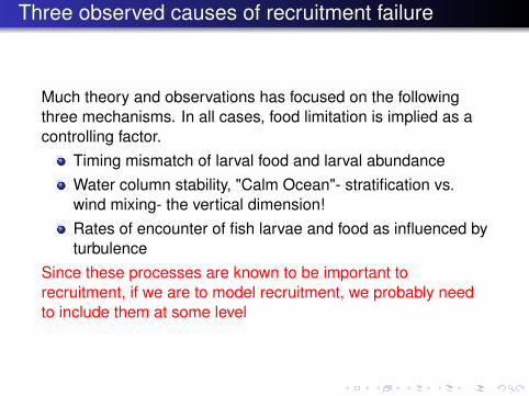
Three observed causes of recruitment failure

Much theory and observations has focused on the followingthree mechanisms. In all cases, food limitation is implied as acontrolling factor.

Timing mismatch of larval food and larval abundanceWater column stability, "Calm Ocean"- stratification vs.wind mixing- the vertical dimension!Rates of encounter of fish larvae and food as influenced byturbulence

Since these processes are known to be important torecruitment, if we are to model recruitment, we probably needto include them at some level

Match/Mismatch Theory: Shepherd and Cushing,1990

Timing is everything

Low stock more affected: higher variabilityMyron Peck

Calm Ocean: [?]

In this case the focus is more on first feeding larvaeA stable water column has nice, possibly subsurfacechlorophyll maximaStable water columns of thin layers of food-rich patchesWind event can mix down the columnInitial feeding of the larvae fails, along with it recruitmentRecruitment variability from a vertical point of viewi/j Lasker event period of calm lasting i days defined bywinds not exceeding jm/s

Turbulence

Feeding by mesozooplankton influenced by turbulence throughseveral mechanisms.

Effects production, concentration and distribution of prey inthe water columnEffects the vertical distribution of individuals (similar toSverdrup theory, young larvae with limited motility arebetter off in well lit (below a threshold) high nutrient areas.Effects the probabilities of encounter, pursuit, and captureof prey by individual larvae

We will focus on the encounter and pursuit aspect

Marine Life at Small Scales

Before looking at larval fish feeding processes, it is important toconsider what life is like at these scales. The key parameter fordescribing the fluid regime experienced by a moving body is theReynolds number:

Re =ULν∼ Inertial Forces/Viscous Forces

where U is the body velocity, L is the body length scale, and νis the kinematic viscosity which for seawater is about 1.15e− 6.

Regimes:0 < Re < 1 : highly viscous, creeping motion1 < Re < 100 : laminar, strong Re dependence........104 < Re < 106 : turbulent, moderate to small Re dependence

Reynolds Numbers and Swimming Speeds (Massel)

Organism Velocity m/s Length m ReBlue whale 10 30 3× 108

Mackeral 3.3 0.3 1× 106

Herring Larvae .02 .01 2× 102

Copepods 0.002 0.001 2× 100

Bacteria 0.00001 0.000001 1× 10−5

Small size = Slow Swimming = Small ReSwimming speeds comparable or smaller than rmsturbulent velocitiesAt Re of about 1, flow is nearly reversible, undulationswimming will not work

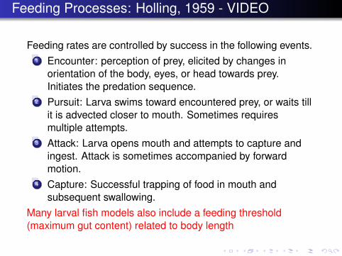
Feeding Processes: Holling, 1959 - VIDEO

Feeding rates are controlled by success in the following events.1 Encounter: perception of prey, elicited by changes in

orientation of the body, eyes, or head towards prey.Initiates the predation sequence.

2 Pursuit: Larva swims toward encountered prey, or waits tillit is advected closer to mouth. Sometimes requiresmultiple attempts.

3 Attack: Larva opens mouth and attempts to capture andingest. Attack is sometimes accompanied by forwardmotion.

4 Capture: Successful trapping of food in mouth andsubsequent swallowing.

Many larval fish models also include a feeding threshold(maximum gut content) related to body length

Feeding: Encounter

Most larval fish are visual feedersWithin a week have fully pigmented eyes and respond tolightLight response (feeding as a function of light) has beenmeasured in rearing tanksLight minimum to feed increases with size.Some studies have found a maximum light levelPause-Travel (P-T), swim ( ∼30s) pause and search (∼1s)(Cod)Cruise predation (continuous swimming, shark style)(Herring)

Feeding: Pursuit, Attack, and Capture

CodAttack posture: L-shapedShort distance of body travel during attackSuck prey into mouth by opening very near to prey

HerringAttack posture - S shapedLonger final attack travel relative to body lengthMove quickly onto prey (aggressive)

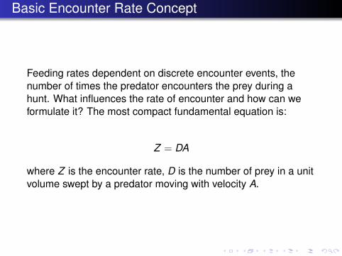
Basic Encounter Rate Concept

Feeding rates dependent on discrete encounter events, thenumber of times the predator encounters the prey during ahunt. What influences the rate of encounter and how can weformulate it? The most compact fundamental equation is:

Z = DA

where Z is the encounter rate, D is the number of prey in a unitvolume swept by a predator moving with velocity A.

Gerritsen and Strickler, 1977

Extended the basic encounter model to include prey swimming

D = πR2N

Predator is cruisingR is contact radiusu is prey velocityv is predator velocityN is prey volumeReactive field is sphericalNo influence from the fluid

Gerritsen and Strickler, 1977

Encounter rate A as a function of predator velocity v and preyvelocity v

A =

{(u2 + 3v2)/3v if v ≥ u(v2 + 3u2)/3u if u ≥ v

Rothschild and Osborn, 1988

Extended the G-S encounter model to include turbulence

Hypothesis: At encounter distances, the rms turbulent velocityw can be as strong or stronger than swimming velocities.Turbulence can influence the encounter rate.

w is related to turbulentdissipation rate εw is also related to separationdistance r . (The closer I am toyou, the less likely you couldbe experiencing a differentvelocity)ε is increased by strong tidalcurrents and wind

Rothschild and Osborn, 1988

Extended the G-S encounter model to include turbulenceEncounter rate A as a function of predator velocity v and preyvelocity v

A =

u2+3v2+4w2

3√

v2+w2if v ≥ u

v2+3u2+4w2

3√

u2+w2if u ≥ v

w > 0 can increase encounterrateincrease larger at smallerprey/predator velocitiessmaller velocities = smalleranimals

Chandresekhar, 1943

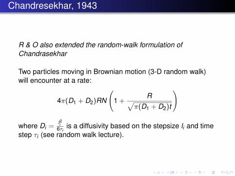
R & O also extended the random-walk formulation ofChandrasekhar

Two particles moving in Brownian motion (3-D random walk)will encounter at a rate:

4π(D1 + D2)RN

(1 +

R√π(D1 + D2)t

)

where Di =l2i6τi

is a diffusivity based on the stepsize li and timestep τi (see random walk lecture).

Rothschild and Osborn, 1988 cont’d

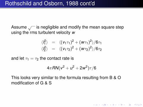
Assume √ is negligible and modify the mean square stepusing the rms turbulent velocity w

〈l21 〉 = 〈(v1τ1)2 + (wτ1)2〉/6τ1

〈l22 〉 = 〈(v1τ2)2 + (wτ2)2〉/6τ2

and let τ1 = τ2 the contact rate is

4πRN(v2 + u2 + 2w2)τ/6

This looks very similar to the formula resulting from B & Omodification of G & S

Rothschild and Osborn, 1988 cont’d

Rothschild and Osborn calculated sensitivity in encounter rateto w as a function of u and v for both modified G-S andmodified random walk schemes. Encounter rates computedusing random walk are more sensitive to turbulence. Why arethe two results different:

G-S is basically swept volume, fish is moving linearly,potential prey come into attack volume base on the size ofthe predator’s sphere and rates of travel of predator andpreyBasically volume of fluid searched or swept is proportionalto the cross sectional area times the velocityIn the random walk formulation, the distance travelled isproportional to

√t rather than t because we are looking at

a diffusive rather than an advective process.Overall conclusion: Contact rates between predator and preyare affected by the kinetic environment: Ingestion is higher inenvironments with higher turbulence

MacKenzie et al, 1994

R & O modeled the effects of turbulence on encounter rates.However, encounter is not everything.Null Hypothesis: Pursuit , attack, and capture are unaffected byturbulence Approach:

Extend R & O to include successful pursuit and combine into aningestion (feeding) probability

P(feed) = P(enc)× P(sp)

where P(enc) is computed using R&O,1988 and P(sp) theprobability of successful pursuit includes processes ofapproach, fixation, and formation of attack position.

MacKenzie et al, 1994 cont’d

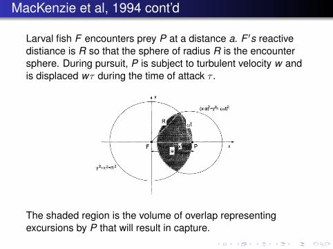
Larval fish F encounters prey P at a distance a. F ′s reactivedistiance is R so that the sphere of radius R is the encountersphere. During pursuit, P is subject to turbulent velocity w andis displaced wτ during the time of attack τ .

The shaded region is the volume of overlap representingexcursions by P that will result in capture.

MacKenzie et al, 1994 cont’d: Assumptions

Larvae use cruise searching strategy (not pause-travel)Requires a minimum time τ to identify, approach, fixate theprey and enter attack postureApproach and fixation require the most time and thus aremost sensitive to turbulenceAttacks only occur in the encounter sphereLarval swimming speed is greater than the preyAttack is unaffected by turbulence. Final attack is normallycarried out from very short distances (10% of body length)where relative turbulent velocities are smallTurbulence induces relative motion between predator andprey

MacKenzie et al, 1994 cont’d: model

Probability of successful pursuit is the ratio of volume of overlap

P(sp) =Vover

Vprey

P(sp) =12

(ρ3 + 1− α) +α

4(α2 − 1)− 3

16α(ρ2 − 1 + α2)2

where α = aωt is the ratio of the distance at which the prey was

first located and the distance prey could be moved byturbulence during attack and ρ = R

ωt is the ratio of reactivedistance to potential prey displacement.

MacKenzie et al, 1994 cont’d: Model Space

dots: excursion sphere, solid circle: encounter sphere

A: no valid solution by assumption, implies encounter distance was greater than reactive distanceB: turbulence cannot move prey out of the pursuit sphere, success guaranteed by assumptionC: encounter sphere is contained in excursion sphere, success is ratio of spheresD: overlap, need expected value of full equation P = f (a, R, ωt) to determine probability

MacKenzie et al, 1994 cont’d: Results

Test out the effects of turbulence from wind mixing on Codlarvae preying on copepods (presumably nauplii). Biologicalquantities from Sundby and Fossum, 1990.

calc ε from wind forcingcalc w from ε

u = 2.0mm/sv = 0.2mm/sR = 6mmτ = 1.7sN = 5/liter

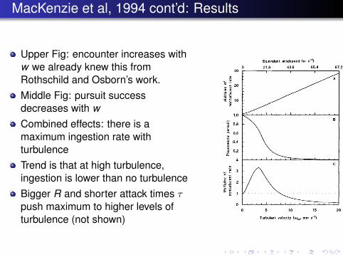
MacKenzie et al, 1994 cont’d: Results

Upper Fig: encounter increases withw we already knew this fromRothschild and Osborn’s work.Middle Fig: pursuit successdecreases with wCombined effects: there is amaximum ingestion rate withturbulenceTrend is that at high turbulence,ingestion is lower than no turbulenceBigger R and shorter attack times τpush maximum to higher levels ofturbulence (not shown)

MacKenzie et al, 1994 cont’d: Thoughts

Inclusion turbulence effects on pursuit results indome-shaped response of ingestion to turbulenceLikely larvae adjust to turbulence (they do). For example,attacking only larger (for bigger R) or more vulnerable (forsmaller τ ) prey.Difficult to measure in field observations: turbulenceeffects patchiness and prey distributions and the strongturbulence required to observed a real maximum coincideswith stormy conditions.Possible issues: Assumed cruise predator, sphericalpursuit volume

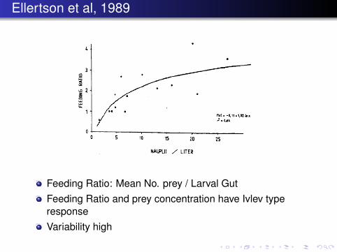
Ellertson et al, 1989

Feeding Ratio: Mean No. prey / Larval GutFeeding Ratio and prey concentration have Ivlev typeresponseVariability high

Sundby and Fossum, 1990

Estimate turbulence at time of observationClassify turbulence levels into discrete categoriesFit Ivlev functions to data falling in discrete turbulencecategoriesR2 > .95

Sundby and Fossum et al., 1990, 1994, 1995,conclusions

Feeding rate of cod larvae off northern norway increasesby a factor of 7 when the wind increased from 2 to 10 m/sEffects of turbulence on larger larvae minimal (swimmingspeeds are larger compared with turbulence velocities)Turbulence-induced contact rate is maximum for slowlymoving first-feeding larvae, as much as 8 times still waterrate.Ingestion rates reach a maximum within normal ranges ofsurface layer turbulenceTurbulence can effect feeding rates up to two months afterhatching

Lough and Mountain, 1996

Collected vertical distributions of haddock/cod larvae inMay, 1981,83Collected wind speed and stratification to calculateturbulence

Lough and Mountain, 1996, cont’d

Got feeding rate from gut contentTurbulence dissipation from windspeed and tidal currentsNo significant regressions forfeeding rate vs. prey concentrationTurbulence effects stronger at lowfood concentrationBuilt contour maps of feeding ratevs. prey conc and turbRidge effect indicates and optimallevel of turb for feeding

MacKenzie and Kiørboe, 1995

M & K performed experiments on herring and cod larvae in atank where they varied turbulence and prey abundance. Theydid not examine pursuit success.

Videotaped fish and measuredPause / Swim TimesAttack Position Rates (APR)

Use models to evaluatereactive distance RModel skill

MacKenzie and Kiørboe, 1995, Conclusions

travel distance between pauses in cod was roughly thesame as reaction distance (in concert with previous theory)at low prey concentrations, APR’s were strongly affectedby turbulencebased on pause/swim times, search behavior wasconsistent (cod = pause/travel ; herring = cruise)Ivlev type saturation of APRs with prey concentration incalm watercod swam more in turbulent water and herring less

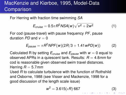
MacKenzie and Kiørboe, 1995, Model-DataComparison

For Herring with fraction time swimming SA

Ecruise = 0.5πR2NSA(w)√

v2 + 2w2 (1)

For cod (pause-travel) with pause frequency PF , pauseduration PD and v = 0

Epause = πR2NPF (w)(2R/3 + 1.41wPD(w)) (2)

Calculated R by setting Ecruise and Epause with w = 0 equal toobserved APRs in a quiescent tank. Results: R = 4.8mm forcod is reasonable given observed swim travel distances.Herring R = 5.7mmUsed R to calculate turbulence with the function of Rothshildand Osborne, 1988 (see Visser and Mackenzie, 1998 for agood discussion of the length scale issue)

w2 = 3.615(εR).667 (3)

MacKenzie and Kiørboe, 1995, Comparison Results

CodObserved increase in APR was 3.2 and 2.2 for small andlarge size classesModel increase in APR was 2.2 and 4.7, similar magnitude,opposite trend

HerringNo statistical change in APR with turbulenceSlight model decrease in APR reflecting changes in pausefrequency and duration with turbulence

Herring, as cruise predators are less effected by turbulence(assuming they don’t modify significantly their strategy)because their swimming velocity is large relative to theturbulence. Pause-travel predators attack from zero velocityand thus their own swimming velocity is not included in themodel.

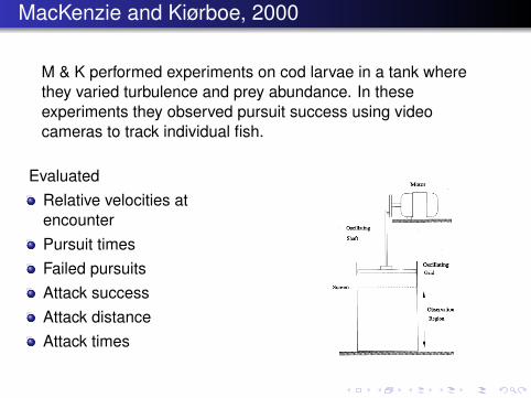
MacKenzie and Kiørboe, 2000

M & K performed experiments on cod larvae in a tank wherethey varied turbulence and prey abundance. In theseexperiments they observed pursuit success using videocameras to track individual fish.

EvaluatedRelative velocities atencounterPursuit timesFailed pursuitsAttack successAttack distanceAttack times

MacKenzie and Kiørboie, 2000, Summary

Turbulent motion reduces the probability that larvae cansuccessfully pursue encountered preyTurbulent velocities where pursuit success was decreasedis comparable to natural turb levels in the surface mixedlayer and mixing fronts.Smallest fish most sensitive to pursuit failures - effects firstfeedingAttack success high at all levels of turbulence - Cod pursueto very small distances (sneak up) and thus relativevelocities are small.Tank study is essentially 0-dimensional, no preypatchiness, no spatial variability of processes. Showed thedomed ingestion -turbulence response under idealconditions. In the open ocean, very difficult to measure.

An Individual-Based Model, Mariani et al., 2007

Goal: investigate feeding of fish in larval environments with acomplex process model