Using GIS Based Property Tax DataFor Trip Generation

Prepared by:

John R. StoneKrista M. Tanaka

Department of Civil EngineeringNorth Carolina State University

Raleigh, NC 27695-7908

and

Alan J. KarrAshish Sanil

National Institute of Statistical SciencesResearch Triangle Park, NC 27709-4006

January 2003

Technical Report Documentation Page

1. Report No.FHWA/NC/2002-28

2. Government Accession No.

3. Recipient’s Catalog No.

4. Title and Subtitle Using GIS Based Property Tax Data for Trip Generation

5. Report DateJanuary 2003

6. Performing Organization Code

Author(s) John R. Stone, Krista M. Tanaka, Alan J. Karr and Ashish Sanil

8. Performing Organization Report No.

9. Performing Organization Name and AddressDepartment of Civil EngineeringNorth Carolina State UniversityRaleigh, NC 27695-7908

10. Work Unit No. (TRAIS)

National Institute of Statistical Sciences19 Alexander Drive (FedEx/UPS)Research Triangle Park, NC 27709-4006

11. Contract or Grant No.

12. Sponsoring Agency Name and AddressNorth Carolina Department of TransportationOne South Wilmington StreetRaleigh, NC 27601

13. Type of Report and Period Covered Final Report July 2000 – December 2001

14. Sponsoring Agency Code2001-08

15. Supplementary Notes

16. AbstractThis project assesses the feasibility of using statistically clustered property tax data instead of windshield survey data for inputinto the Internal Data Summary (IDS) trip generation model used by the North Carolina Department of Transportation. Thereport summarizes the clustering analysis and its data requirements. To gauge clustering resource requirements for a case studyapplication, NCSU researchers examine the Town of Pittsboro. Comparing the traffic flow outputs of the traditional modelingtechniques and those resulting from the use of the clustering method to 56 ground count stations, the research finds that clusteringand tradition methods yield similar results. An 85% reduction in man-hours required to gather the input data is the main benefitresulting from the use of the clustering technique. The major drawback is that advanced statistical training is required toimplement the technique.

17. Key WordsTraffic Forecasting, GIS, Trip Generation, k-meansClustering

18. Distribution StatementUnlimited

19. Security Classif. (of this report)Unclassified

20. Security Classif. (of this page)Unclassified

21. No. of Pages81

22. Price

Form DOT F 1700.7 (8-72) Reproduction of completed page authorized

iii

Disclaimer

The contents of this report reflect the views of the authors and not necessarily the views of theUniversity. The authors are responsible for the facts and the accuracy of the data presentedherein. The contents do not necessarily reflect the official views or policies of the North CarolinaDepartment of Transportation or the Federal Highway Administration at the time of publication.This report does not constitute a standard, specification, or regulation.

Acknowledgements

The authors would like to express thanks to the North Carolina Department of Transportation(NCDOT) and the Federal Highway Administration (FHWA) for sponsoring this research and theInstitute of Transportation Research and Education (ITRE) for administering the project. A thankyou as well, goes to the Research Project Steering Committee (RPSC), including, Mike Stanley,David Hyder, Leta Huntsinger and Joe Stevens.

A special thanks is extended to Billy Smithson and Jamal Alavi of the NCDOT and Felix Nwokofrom the City of Durham for their technical support throughout the project.

iv

TABLE OF CONTENTS

TABLE OF CONTENTS ...........................................................................................................................................IV

LIST OF TABLES .......................................................................................................................................................VI

LIST OF FIGURES................................................................................................................................................... VII

EXECUTIVE SUMMARY....................................................................................................................................ES-1

1. INTRODUCTION.................................................................................................................................................1

BACKGROUND.............................................................................................................................................................. 2Trip Generation and the Four-Step Process ....................................................................................................2Trip Generation Methods....................................................................................................................................3Internal Data Summary........................................................................................................................................4

PROBLEM DEFINITION................................................................................................................................................ 4SCOPE AND RESEARCH OBJECTIVES......................................................................................................................... 5CHAPTER SUMMARY .................................................................................................................................................. 5

2. LITERATURE REVIEW ....................................................................................................................................6

REVIEW OF DESIRABLE GIS MODEL CHARACTERISTICS...................................................................................... 6NCDOT Use of GIS...............................................................................................................................................6Portland Metro’s GIS Database (FHWA, 1998a)...........................................................................................7CAMPO Automated Data Summary...................................................................................................................8

METHODS OF ANALYSIS............................................................................................................................................. 8CHAPTER SUMMARY .................................................................................................................................................. 9

3. A RESEARCH METHODOLOGY FOR TRIP GENERATION..........................................................10

4. HOUSEHOLD CONDITIONS BASED ON PROPERTY TAX.............................................................13

CLASSIFICATION METHODOLOGY .......................................................................................................................... 13VARIABLE SELECTION.............................................................................................................................................. 13CLASSIFICATION TECHNIQUES................................................................................................................................ 16

Classification Tree..............................................................................................................................................16Linear Discriminant Analysis ...........................................................................................................................17Clustering of Households..................................................................................................................................17

DISCUSSION OF FINDINGS......................................................................................................................................... 18CHAPTER SUMMARY ................................................................................................................................................ 19

5. THE PITTSBORO CASE STUDY..................................................................................................................21

PITTSBORO MODEL DEVELOPMENT ....................................................................................................................... 21BASE YEAR DATA COLLECTION ............................................................................................................................. 22PITTSBORO GIS DATABASE..................................................................................................................................... 24

Parcel Level Database.......................................................................................................................................24Aggregated TAZ Level Database .....................................................................................................................25Network Database ..............................................................................................................................................26

INTERNAL DATA SUMMARY.................................................................................................................................... 26STATISTICAL COMPARISONS.................................................................................................................................... 27RESULTS..................................................................................................................................................................... 28DISCUSSION................................................................................................................................................................ 33CHAPTER SUMMARY ................................................................................................................................................ 34

6. CONCLUSIONS AND RECOMMENDATIONS.......................................................................................35

STATISTICAL CLASSIFICATION................................................................................................................................ 35

v

GIS PROPERTY TAX DATABASE ............................................................................................................................. 36THE PITTSBORO CASE STUDY ................................................................................................................................. 37SUMMARY RECOMMENDATIONS............................................................................................................................. 38RECOMMENDED METHODOLOGY FOR USE OF CLUSTERING.............................................................................. 38

7. REFERENCES .....................................................................................................................................................39

APPENDIX A CALCULATION OF NON-HOME BASED, NON-RESIDENT SECONDARY TRIPSFOR HHC AND CLUSTER SCENARIOS ..................................................................................................41

APPENDIX B SAMPLE PARCEL DATABASE FILE....................................................................................43

APPENDIX C SAMPLE TAZ DATABASE FILE.............................................................................................44

APPENDIX D SAMPLE NETWORK DATABASE FILE...............................................................................45

APPENDIX E IDS INPUT FILE FOR HHC METHOD..................................................................................46

APPENDIX F IDS INPUT FILE FOR CLUSTER METHOD.......................................................................50

APPENDIX G NCDOT BASE YEAR PROCEDURE FOR PITTSBORO (SMITHSON, 2001)..........54

APPENDIX H STATISTICAL COMPARISON OF PRODUCTIONS AND ATTRACTION:CALCULATIONS ...............................................................................................................................................57

APPENDIX I STATISTICAL COMPARISON OF ASSIGNED FLOWS AND GROUND COUNTS:CALCULATIONS ...............................................................................................................................................65

vi

LIST OF TABLES

Table 1-1: Cross-Classification Model for Daily Home-Based Other Vehicle Trips ......................................... 3

Table 1-2: IDS Daily Vehicle Trip Generation Rates by Household Condition . ................................................ 4

Table 2-1: NCDOT GIS Benefits and Costs on Selected Projects . ....................................................................... 7

Table 4-1: Comparison of Statistical Models Used to Classify Property Tax Data for Input into TripGeneration Model...................................................................................................................................... 19

Table 5-1: Employment Categories by SIC Code ................................................................................................... 23

Table 5-2: IDS Daily Vehicle Trip Generation Rates by Household Condition Rating Used in PittsboroStudy ...........................................................................................................................................................26

Table 5-3: Results of the Comparison of Total Productions and Total Attractions Between Models ............28

Table 5-4: Results of the Comparison Between the HHC Model and the Cluster Model by TripPurpose.........................................................................................................................................................29

Table 5-5: Production Results and Differences Between the HHC Model and the CLUSTER ModelBy Trip Purpose....................................................................................................................................30-31

Table 5-6: Results of the Comparison Between Link Assignments for the HHC Model, CLUSTER Modeland Ground Counts.................................................................................................................................... 32

Table 5-7: Required Data Compilation Times for the HHC and CLUSTER Methods ....................................34

vii

LIST OF FIGURES

Figure 1-1: NCDOT Travel Model Development Process....................................................................................... 2

Figure 3-1: Methodological flow chart....................................................................................................................... 11

Figure 4-1: Distributions of the Predictors (log scale) for Each HHC.................................................................. 15

Figure 4-2: Pairwise Scatterplots of the Predictors.................................................................................................. 16

Figure 5-1: Vicinity Map of Pittsboro, NC (Not to Scale) ...................................................................................221

Figure 5-2: Pittsboro Study Area with Parcels and Right-of-Way........................................................................ 22

Figure 5-3: Household Rating by Parcel.................................................................................................................... 24

Figure 5-5: CLUSTER Method Daily Flow Map..................................................................................................... 32

Figure 5-6: HHC Method Daily Flow Map............................................................................................................... 33

ES-1

EXECUTIVE SUMMARY

A strong relationship exists between property characteristics like tax value and tripgeneration according to recent travel surveys by USDOT and other agencies. Suchproperty information is now common in geographic information system (GIS) format.GIS data are available at city and county planning agencies across North Carolina, andthe GIS data potentially offer a relatively inexpensive, quick method for estimating tripgeneration for regional travel models.

Currently, the NCDOT model called the internal data summary (IDS) for trip generationrelies on “drive-by” windshield observations of household condition to estimate travelespecially for residential locations. Windshield surveys however, have severalweaknesses.

• They are expensive and time consuming;• They depend on subjective judgments that are hard to replicate and that may lead

to errors and bias; and• They cannot be forecast to the future.

Consequently, the question arises: Can property tax data replace windshield surveysto estimate travel in IDS? If the answer to this question is “yes”, then statisticalcategorization of GIS data can replace expensive, time consuming and potentially errorprone windshield surveys by relatively easily acquired property tax information. Thisresearch will attempt to answer this question.

Keeping trip generation tied to readily available property tax data is the key to costeffective data collection. First, the NCSU approach develops a method to classifyproperty tax data into the common household categories designated in windshieldsurveys. Second, the approach compares IDS trip generation and resulting travelestimates to the same results produced using GIS data. In addition, ground counts servesto validate the results of both methods.

For Pittsboro, this project will determine if property tax information can be used in placeof windshield surveys for household condition. If so, a workable method for collectingproperty tax information and merging it to the base year trip generation model will beproposed for other cities.

More specifically the objectives of this report are:• To determine an appropriate statistical method to classify dwelling units by GIS

based property tax data;• To suggest a database structure that includes all of the required fields for use in the

new classification procedure for trip generation; and• To demonstrate the application of the new classification method using the case study

city of Pittsboro, NC;

Ultimately the goal is to simplify the data collection process and to reduce the uncertaintyin data input for the trip generation model used by NCDOT.

ES-2

Statistical Classification

This project has as a goal to determine a method for grouping and classifying GIS basedproperty tax data into categories for use in the IDS trip generation model. The NationalInstitute of Statistical Sciences (NISS) determine that deed acres, improvement valuesand land values are the three best predictors of household condition (HHC). Using thesethree variables, NISS carefully reviews the various statistical techniques [LinearDiscriminant Analysis (LDA), Classification and Regression Trees (CART) and k-meansclustering] available for this type of categorization and settles on the k-means clusteringmethod. The reasons for selecting k-means clustering as the preferred method areoutlined below.

K-means clustering groups properties into clusters based on natural breaks in the dataanalogous to household condition categories. Clusters are assigned to properties based onthe statistical similarity between the property tax characteristics of the land parcels.Parcels with similar characteristics are grouped into the same cluster. For a case studybased on Pittsboro, N.C., the clusters are used instead of HHC ratings for single familydwelling units for the purpose of trip generation. The demonstrated advantages of thismethod are that:

• Properties can be assigned cluster values without the subjective evaluation of HHCsduring drive-by windshield surveys;

• Clusters are not based on HHC ratings as is the case with the CART and LDAapproaches;

• Clustering does not require any windshield survey to be done.

The disadvantage to the k-means clustering approach is that a new clustering would haveto be performed for each city. The amount of statistical training needed is quitesubstantial and so the NCDOT would have to hire a statistician or train some of theiremployees to carry out the analysis.

One of the challenges of the statistical analysis is to balance complexity versusgeneralizability of the clustering model. In doing so, the predictive power of theclassification tool is often limited. In this case, the limitation is to some extent due to theinherent subjectivity of the HHC assignment obtained in a windshield survey. However,the primary reason for the limited predictive power of each of the classification tools isthat the property tax data contain only part of the information used to assign HHCs. Thesurveyors in the field subjectively incorporate several other items of information such asnumber of vehicles on the premises and neighborhood information in making a HHCassessment. This extra information is not captured in the property tax data and could helpto increase the predictive power of the k-mean clustering model. One recommendation isto incorporate automobile ownership and numbers of persons by age group into the GISdatabase for use in a clustering procedure.

ES-3

GIS Property Tax Database

There are several advantages to using GIS based tax data for travel forecasting:• GIS based property tax data are available for most N.C. cities;• Property tax data is regularly collected and updated by N.C. counties; and• Trip generation based on GIS property tax data is reproducible because of its

quantitative basis.Thus a second objective is to recommend a GIS database structure. In order to useproperty GIS based property tax data in a meaningful way for trip generation purposes, itis essential to design a database that completely incorporates all of the necessaryattributes for the study area. In the case study city for this project, Pittsboro, N.C., NISSdiscovered a number of parcels that were missing part or all of the property tax data (deedacres, improvement value and land value) required to classify the parcels using thestatistical procedures they identified.

Maintaining a complete, up to date parcel level database file for each study area isessential. Furthermore, it would facilitate data compilation if there were statewide GISstandards for coding parcel information (PINs, etc.). A standard format is essential forjoining information from external databases into the GIS parcel layer. It allows plannersto adjust TAZs boundaries as conditions change. TAZ level database files can be builtusing TransCAD based on the TAZ field in the parcel level database. Recommendedfields to include in a parcel level database used for k-means clustering are as follows:

Area Area of ParcelPerimeter Perimeter of ParcelPIN Parcel Identification NumberLand_FMV Tax value of land (base year)IMPR _FM Tax value of Improvement (base year)DEED_A Acreage of parcelLU_Parcel Land use or type of propertyTAZ Assigned TAZMTAZ Census TAZ number used in Regional ModelINDEMP Number of employees in Industrial employmentRETEMP Number of employees in Retail employmentHWYEMP Number of employees in Highway Retail employmentOFFEMP Number of employees in Office employmentCLUSTER1 Number of households in the first cluster on parcelCLUSTER2 Number of households second cluster on parcelCLUSTER3 Number of households in third cluster on parcelCLUSTER4 Number of households in fourth cluster on parcelCLUSTER5 Number of households in fifth cluster on parcel (incorporate additional

fields for study areas with more than 5 clusters)

ES-4

The Pittsboro Case Study

The third objective of this project is to test the chosen statistical classification method forthe case study town of Pittsboro. Both standard HHC input data and CLUSTER databased on GIS property tax data are used in the four-step travel demand model forPittsboro to test the results of the traditional HHC method to the CLUSTER method. Theoutputs of the trip generation step are compared using a t-test. Assuming the zonalproductions from the two different methods are considered a paired sample, thedifference between trips produced by each zone is calculated. The resultant differencesfor each zone become a single sample of differences about which inferences can be made.The null hypothesis is that there is no difference between trips resulting from the HHC orCLUSTER input data. Therefore, the mean of the sample of differences is compared to anexpected mean (µD) of zero using a one sample t-test. The test demonstrates that theproductions and attractions produced by the two methods do not compare well for the twomodels at a 95% confidence level. However, the mean difference between productionsfor the HBW and NHB trip purposes are quite low. The mean difference for the HBW is3.69 productions per TAZ between the two models and 2.76 for the NHB productions. Inpractical application of the trip generation model these differences are negligible. Thesame trend is documented for the attractions

Since the most important validation of a model compares traffic ground counts toestimated traffic, a comparison of flows versus ground counts is also undertaken for bothmethods. A comparison of the pre-calibration HHC and the CLUSTER models shows amean percent difference between ground counts and link assignments greater than 25%which is well above the acceptable limits for calibrated NCDOT models. Mean percentdifference between ground count and flows for the HHC model is greater than that foundusing the CLUSTER model. The CLUSTER model also results in a slightly better groundcount to flow ratio than does the HHC model. Both models have the same 26 links withflow rate error within acceptable ranges. These results indicate that the pre-calibrationflows derived using the CLUSTER method are no less accurate than those obtained usingthe HHC model. Statistical differences between CLUSTER model flows and groundcounts are likely an issue that can be dealt with in the calibration phase of modeling. Ifthe HHC model can be calibrated then the CLUSTER model should also be able to becalibrated and percent differences brought within acceptable limits. This indicates thatCLUSTER model data, based on GIS property tax information, is no less accuratean input to IDS than is the windshield survey data.

The benefit of using the CLUSTER model is the timesaving associated with its use. Thewindshield survey of Pittsboro took 104 person-hours to complete the 100% evaluation ofhouseholds. Obtaining the GIS data from Chatham County required no more than a 10-minute telephone conversation but did require some data cleansing efforts beforeapplying the NISS clustering method. Data cleansing involves reducing the completeparcel level data down to a data set that only includes single family dwelling units withparcel identification number, deed acre, improvement value and land value attributes. TheNISS clustering model is not very straightforward and requires significant statisticalknowledge to be able to apply it to a GIS property tax data set. Total classification with

ES-5

the CLUSTER method, including data cleansing, would require 8-16 person hours (oncethe procedure is understood). When compared to the 104 hours required to complete awindshield survey, the CLUSTER model takes only 15% of the time to implement.

Overall, the CLUSTER model used to evaluate property tax data looks promising interms of timesaving. The major drawback is in the statistical training required toimplement the procedure for each city or town.

Conclusions and Recommendations

GIS based property tax data that is freely available and regularly updated is an attractivealternative to special drive-by windshield surveys of all households in a community forwhich a travel model is being prepared. Significant time and expense savings arepossible, plus GIS property tax data (including property type, size, and value) arequantitatively recorded in database format and compatible with travel forecastingsoftware like TransCAD.

Adapting GIS property data for a case study to city traffic analysis zones is not difficultusing GIS techniques. However, statistically grouping GIS property tax data in a mannersimilar to conventional observations of household condition (an acceptable surrogate fortrip generation potential) obtained in a windshield survey is difficult. A sophisticatedstatistical technique called k-means clustering is the preferred technique (compared toLDA and CART) to group property tax data instead of the subjective assignment of casestudy household conditions. The resulting property tax clusters (similar to householdcondition categories used in IDS, the NCDOT trip generation software) estimate pre-calibration trip productions and attractions that are statistically different at the 95%confidence level from productions and attractions generated by IDS using windshieldsurvey data.

The comparison of pre-calibration link volumes to actual ground counts for both GISbased trip generation and windshield survey shows that GIS based trips estimate aresomewhat better than the windshield survey based estimates. Overall, for pre-calibratedresults, the GIS based productions, attractions and link volumes are no less accurate thanpre-calibration windshield survey results. Yet, the GIS based data are obtained 85% morequickly and less expensively than windshield survey data for the case study city (actualmodeling time remains the same for both scenarios).

The specific recommendations for NCDOT, resulting from this project follow:1. Test the use of GIS based property tax data in another North Carolina city.2. Enrich the property data with other data like vehicle ownership and census data to

enhance the predictive power of the k-means clustering classification tool.3. Conduct the comparisons of productions, attractions and link volumes on calibrated

models.4. Obtain software and tutorial guides so that NCDOT staff can become familiar with k-

means clustering.

ES-6

5. Contact county tax departments and discuss data format and data items that areneeded for travel forecasting.

1

1. INTRODUCTION

A strong relationship exists between trip generation and property characteristics like taxvalue according to recent travel surveys (FHWA, 1998a; NuStats International, 1995).Property information is now common in geographic information system (GIS) format.GIS data are available at city and county planning agencies across North Carolina and theGIS data potentially offer a relatively inexpensive, quick method for estimating tripgeneration for regional travel models.

Currently, the NCDOT trip generation model called the internal data summary (IDS)relies on “drive-by” windshield observations of household condition to estimate travelespecially for residential locations (NCDOT, 1999). Windshield surveys have severalweaknesses.

• They are expensive and time consuming;• They depend on subjective judgments that are hard to replicate and can lead to

bias and errors; and• They cannot be forecast to the future.

By contrast, GIS property tax data are inexpensive, accurate, up to date and can beprojected into the future. Moreover, GIS allows these data to be used readily in analysisand to produce visual descriptions. Consequently, the question arises: Can property taxdata replace windshield surveys to estimate travel in IDS? If the answer to thisquestion is “yes”, then statistical categorization of GIS data can replace expensive, timeconsuming and potentially error prone windshield surveys by relatively easily acquiredproperty tax information. This research will attempt to answer this question.

Keeping trip generation tied to existing property tax data is the key to cost effective datacollection. First, the NCSU approach develops a method to classify property tax data intothe common household categories designated in windshield surveys. Second, theapproach compares IDS trip generation and resulting travel estimates to the same resultsproduced using GIS data. In addition, ground counts serve to validate the results of bothmethods.

Although a GIS based method could be used for determining data input for tripgeneration in general, the NCSU project uses the NCDOT IDS trip generation model.While NCDOT primarily associates IDS with Tranplan and smaller city models, theNCSU approach can be adapted to TransCAD, which is becoming the preferred modelingtool at NCDOT. In the meantime, Tranplan models will continue in use for several years.

To provide background, this report describes the traditional four-step travel forecastingprocess and the trip generation step that is the focus of this effort. In particular the reportdiscusses trip generation by IDS. Next, the report refines the problem based on thebackground statement and identifies the research objectives. Then the report developsand justifies the research approach through a review of pertinent literature. Throughout,the report emphasizes the significance to NCDOT of the proposed GIS-based datacollection method for household data.

2

Background

Trip Generation and the Four-Step Process

NCDOT planners and engineers develop long range, regional travel forecasts by applyingthe “traditional” four-step planning process: 1) trip generation, 2) trip distribution, 3)mode split, and 4) trip assignment as seen in Figure 1-1. For the past decade or more,they have implemented the process with Tranplan (Urban Analysis Group, 1995).Recently, however, they have adopted TransCAD (Caliper Corporation, 2000), and theyare converting their regional models from Tranplan to the new, more GIS-orientedenvironment that TransCAD offers.

IDS

Internal Data Summary)

TRIP DISTRIBUTION

MODE CHOICE

TRIP ASSIGNMENT

FIELD DATA

Dwelling Untis by ClassEmployment by GroupExternal Station Productions

TRIP GENERATION PARAMETERS

Persons per DUGeneration Rates by DU TypeOccupancy Rates by DU TypeAttraction Factor EquationsNHBsec ProductionsPercent InternalTrip Percentages by Purpose

(Trip Generation and

Base Year

Network

CALIBRATION

Figure 1-1: NCDOT Travel Model Development Process (NCDOT, 1997).

This research focuses on the first, and arguably the most important and costly, step of thetravel forecasting process – trip generation. Trip generation estimates the regionaldemand for travel. If the estimate is wrong, the regional model is wrong (garbage in,garbage out). Furthermore, the estimate for regional travel demand is very data intensive,potentially very expensive, time-consuming, and uncertain. To estimate regional travel inthe base year analysts must collect current socioeconomic data for each land use parcel ineach traffic analysis zone (TAZ) in the region.

3

For both the base year and the future year, the trip generation step estimates the numberof trips produced by and attracted to each TAZ based on zonal residential and businessland use. Each TAZ is characterized by associated socioeconomic data such as dwellingunits and condition, employment, and commercial vehicles. The generation procedureconsists of three basic functions: computing total trips produced by a zone, computingtotal trips attracted to a zone, and scaling to equate the total productions and the totalattractions in the region for each of several trip purposes.

Trip Generation Methods

Generally speaking there are three methods to estimate trip generation – regressionmodel, cross-classification and trip rates. Some transportation planning agencies usecross-classification models based on samples of household travel behavior data toestimate zonal trip productions, and they use regression models to estimate zonal tripattractions. Other agencies use sophisticated regression models for generatingproductions as well as attractions. Recently, activity-based methods for trip generationhave also been implemented (Stone, et al, 2000).

Cross-classification involves using sample interview data to construct tables of variablesdescriptive of dwelling units (i.e. occupancy, auto ownership, household income, etc.)and the travel behavior (daily vehicle or person trip rates) for the different classes ofdwelling units. Such a table is shown in Table 1-1. Knowing the number of dwellingunits in each income class in each zone will give the number of daily trips for that zone.Summing over all zones will give the trips for the entire study area. Travel for varioustrip purposes (home-based work, home-based other, and non-home-based) are determinedsimilarly for both the base and future year.

Table 1-1: Cross-Classification Model for Daily Home-Based Other Vehicle Trips (NCDOT, 1997).

Persons perDwelling Unit

Income Group

1 2 31 0.28 0.85 1.442 1.25 2.26 2.70

3 or more 1.33 2.46 3.21

An advantage of cross-classification is the transferability of the model from zone to zonein the study area and between cities of similar types. The model can discriminate amongmany socioeconomic categories (nine in this example). Also, cross-classification canshow realistic non-linear effects in travel behavior. On the other hand, cross-classification models have complex relationships among the data that lead to moredifficult, less intuitive model calibration. Furthermore, cross-classification typicallydifferentiates trip-making potential within a TAZ based on zonal averages from sampledata. The samples may be as few as 30 per category depending on city size. Perhapsmost troublesome is the difficulty in estimating future income.

4

Internal Data Summary

Besides cross-classification NCDOT engineers and planners use IDS, which uses triprates for different residential and employment types to estimate trip generationproductions and attractions. They developed IDS in-house, and it is separate from, butcan be merged with, Tranplan (Urban Analysis Group, 1995) and TransCAD (Caliper,2000). IDS relies on average, time invariant trip rates for North Carolina cities. The triprates are the coefficients of the IDS model for trip productions and attractions. Duringmodel validation, the trip rates are changed as necessary to improve the comparison ofestimated link volumes versus actual ground counts.

For productions there are five trip rates corresponding to five household conditioncategories – excellent, above average, average, below average, and poor (Table 1-2).Trip rates for special residential categories like university dormitories are also included.Given the number of households by condition in a TAZ, IDS determines the number ofdaily home-based productions in the TAZ by trip purpose. Area-wide productions by trippurpose result from summing the individual TAZ productions. The IDS output includes afile containing summaries of household conditions by TAZ, productions and attractionsfor each TAZ by trip purpose and area-wide totals by trip purpose.

Table 1-2: IDS Daily Vehicle Trip Generation Rates by Household Condition (NCDOT, 1999).

HouseholdCondition

Excellent AboveAverage

Average BelowAverage

Poor

Trip Rate 12.0 10.0 8.0 6.0 4.0

IDS has certain strengths compared to cross-classification. First, trained techniciansinspect every household in a TAZ. Sampling is not used, and thereby every home-basedtrip generator is counted. They make a visual assessment of the condition of eachhousehold, and they assign it to one of the five household conditions based on suchfactors as observed numbers of vehicles, the estimated number of occupants, evidence ofchildren, and estimated property value versus local averages. In this regard, IDS has thediscrimination of cross-classification. Second, since IDS is like a linear regressionmodel, its use is relatively straightforward and intuitively easy to understand. On theother hand, IDS assumes consistent and accurate appraisals of household condition by theinspectors. Moreover, inspecting every property, while avoiding the uncertainties ofsampling, leads to costly, time-consuming data collection.

Problem Definition

As discussed above, NCDOT has a daunting task to periodically count every householdand appraise its condition in order to develop base year trip generation estimates for aregion. The housing count is made by trained technicians who drive by each property inthe city, identify it as residential, and classify its condition based on visual appearance,apparent number of occupants including children, and parked vehicles. Clearly, such

5

counts and subjective appraisals made while driving by a property are prone to error andbias.

This research tests the hypothesis that property tax data can replace windshield surveydata. Analysts could then replace the cumbersome and error-prone, inspection-basedcounts and condition estimates of each household in each TAZ with computer-basedproperty tax data of each property in a TAZ. If the hypothesis is true, this report willpropose recommendations for appropriate data collection procedures and discuss how toadapt IDS for trip generation based on property tax information.

Scope and Research Objectives

The scope of this project addresses the trip generation of the case study Town ofPittsboro, North Carolina. This city has all of the required information: IDS windshieldsurvey data (year 2000), base year trip generation results corresponding to the windshieldsurvey data (IDS output), GIS parcel data and corresponding property tax records and theNCDOT travel model developed with TransCAD.

For Pittsboro, this project will determine whether property tax information can be used inplace of windshield surveys for household condition. A workable method for mergingproperty tax information to the base year trip generation model will be proposed.

More specifically the objectives of this report are:• To determine an appropriate statistical method to classify dwelling units by GIS

based property tax data;• To suggest a database structure that includes all of the required fields for use in the

new classification procedure; and• To demonstrate the application of the new classification method using the case study

Town of Pittsboro, NC.

Ultimately the goal is to simplify the data collection process and to reduce the bias in datainput for the trip generation model used by NCDOT.

Chapter Summary

The NCDOT realizes that the windshield survey method for collecting socio-economicdata for input into IDS for trip generation has several shortcomings. Besides being timeconsuming and inefficient, it is based on subjective evaluation and hence it is notreproducible. With the advances in GIS in the past few years, and the ready availabilityof property tax data that each county prepares, it makes sense to move toward a methodfor household classification based on a more reproducible evaluation.

The following chapter will justify a GIS-based approach. Subsequent chapters will, inturn, summarize a methodology for developing a GIS approach and apply the approach tothe case study Town of Pittsboro, NC. Recommendations and conclusions regarding theeffectiveness of using GIS data for Pittsboro trip generation will close out the report.

6

2. LITERATURE REVIEW

Many cities and agencies including NCDOT use GIS databases for a range of land useand transportation planning activities (Shinebein, 1999; He, 1999; FHWA, 1998a;FHWA, 1998b). However, the applicability of GIS based land use data like propertyvalues, type and location; have not been demonstrated for travel forecasting. Forexample, the Capital Area Metropolitan Planning Organization (Raleigh, NC) could notfind a strong statistical correlation between land use and socioeconomic data available inGIS format and travel behavior (Parsons Transportation Group, 2000). While findingsuch relationships seems intuitively plausible, issues such as GIS and travel survey dataavailability, GIS data format and accessible statistical methods complicate the problem.The following literature review briefly describes NCDOT’s use of GIS, PortlandMETRO’s use of GIS, the CAMPO GIS study and alternative statistical methods forestablishing relationships between GIS land use data and travel behavior data. Theresults of the literature review help establish the research approach that a subsequentchapter describes.

The motivation for the proposed trip generation project comes from the need to facilitatesocioeconomic data collection, reduce its cost and improve its accuracy. The keytechnology that makes this project feasible is GIS – geographic information systems.

More and more NCDOT is using GIS to support decision-making. TransCAD, theprimary NCDOT urban transportation planning software, has full GIS capabilities.NCDOT also uses GIS to locate and describe highways and their features including signs,pavement conditions and accidents through the Linear Referencing System.

Review of Desirable GIS Model Characteristics

NCDOT Use of GIS

The GIS Unit at the NCDOT compiles environmental GIS data and supplements it withsome field surveys of historic sites (FHWA, 1998b). Using relatively inexpensivecommercial software like ArcView, engineers overlay GIS coverages on aerialphotography to produce map-based data that are used for public hearings and as part ofthe approval process (FHWA, 1998b). This overlay technique is helpful in evaluating thedifferent improvement scenarios as their effect on various environmental resources canbe visualized.

Besides ArcView, NCDOT has adopted the network travel forecasting tool calledTransCAD, which relies heavily on GIS data input and GIS graphical output. NCDOT iscontinuing to expand its GIS applications to traffic operations, safety and maintenance.As a result, the Federal Highway Administration Travel Model Improvement Programhas recognized NCDOT’s innovation in GIS by featuring the Statewide Planning Unit asone of six planning agencies that extensively uses GIS. In the report Transportation

7

Case Studies in GIS the FHWA describes “NCDOT: Use of GIS to SupportEnvironmental Analysis During System Planning”. Of particular interest are the benefitsand costs that accrue from using GIS (Table 2-1). NCDOT reports that GIS collectionand analysis of environmental data (which is similar to the process proposed forsocioeconomic data in this report) is more efficient, quicker, less costly and improves thecommunication and consensus process between the Department, regulatory agencies andthe public.

Table 2-1: NCDOT GIS Benefits and Costs on Selected Projects (FHWA, 1998b).

Project Benefits CostsHalstead Blvd - Environmental Assessment (EA) reduced by 16

months.- Cost savings $150,000.

- GIS data collection, 3months.

- Cost $15,000.

MorgantonConnector

- Early consensus, minor EA not major EA.- Cost savings $250,000.

- GIS documentation- Cost $20,000

Portland Metro’s GIS Database (FHWA, 1998a)

Portland Metro is the regional government and the MPO that serves 1.3 million people inClackamas, Multnomah and Washington Counties in Oregon. Metro provides all of theurban transportation planning for the region. Metro is the leading user of GIS-T fortransportation planning in the country. The Data Resources Center (DRC) is the in-housedepartment that is responsible for gathering base year data, producing forecasts andmanaging the database and GIS.

Portland Metro is recognized for its innovations in using GIS for activity-based modelssuch as Transims (Los Alamos, 1999). Of particular interest to this research project is thePortland Metro use of GIS to store data using households as the unit of analysis. WhilePortland Metro uses a more disaggregate model than NCDOT does, the GIS lessonslearned and benefits accrued are important for this research and eventual application inTransCAD. The benefits of storing both household and employment data at thedisaggregate level are clear. When using TAZs as the unit of analysis, but storing data atthe parcel level, it is simple to adjust TAZ boundaries when needed without concernsabout losing data. Furthermore, data stored at the disaggregate level allows for datagroupings other than standard TAZs (smaller TAZs can be created within a TAZ forsmaller scale planning projects). Although the NCSU GIS database is stored in apolygon coverage based on parcels, a disaggregate format is maintained.

The GIS is known as the Regional Land Information System (RLIS). It stores 75 layersof demographic, employment, environmental and transportation data for the region in theform of polygon, arc and point coverages. The base maps and attribute data arecontinually updated and published quarterly in CD-ROM format. The GIS is maintainedusing ESRI’s Arc/INFO software.

8

The Metro trip generation model uses disaggregate demographic data stored as point datarecords within the GIS. The point data represents separate survey data that have beengeocoded to the address from which they were received. Regional disparities withintravel analysis zones can then be taken into consideration during the trip generation phaseof transportation planning. Employment information is also entered as point data withinthe GIS.

Metro decided that GIS would be an integral part of their planning process. They haveinvested a good deal of money to create and maintain such an elaborate database.Metro’s “GIS-centric” approach to planning requires many resources to maintain it.

CAMPO Automated Data Summary

Closer to home, the Capital Area Metropolitan Planning Organization (CAMPO) hasinitiated an extensive GIS data collection effort. The project is called the AutomatedData System (ADS) (CAMPO, 1999). Its goal is to capture in GIS format all public datathat will support the land use and transportation planning efforts of municipalities inWake County. Significantly for this research project, the data will include parcelinformation from tax records. Other data will include employment and income data,business locations by Standard Industrial Code (SIC), water and sewer billings, vehicletax billings, etc. by address.

The CAMPO ADS study found a weak statistically significant relationship betweenproperty tax variables and household trip production rates. The study did show thathousehold composition is the fundamental determinant of trip production and that land-use and dwelling unit characteristics were not reliable predictors of travel behavior(Parsons Transportation Group, 2000).

Methods of Analysis

The primary analytical tasks of this project are (1) to determine if GIS property taxrecords can be substituted for windshield survey household condition ratings and if so,(2) to accurately estimate the trip generation and network traffic in Pittsboro, the casestudy city. Task (2) will be accomplished using IDS and TransCAD as discussedpreviously. Task (1), however, requires selection of an appropriate statistical method.

For finding similar travel behavior relationships, the CAMPO study applied standardcross-classification and regression/ANOVA methods from commonly available softwarelike spreadsheets, SAS and SPSS. Analysis was straightforward, though the results werenot encouraging. Property tax data evaluated as possible causal variables included heatedsquare footage, dwelling unit ownership status, type-and-use classification, number ofrooms, acreage, appraised tax value, own or rent and type of home (ParsonsTransportation Group, 2000). Heated square footage and type-and-use classificationshave the strongest relationship to overall trip production.

9

Other more sophisticated statistical approaches exist for determining clusteredrelationships similar to those implied by the five standard IDS household conditions fortrip generation. In one study, North Carolina State University (NCSU) and the NationalInstitute of Statistical Sciences (NISS) examined relationships between air quality and avariety of variables including traffic descriptors, a site variable, and vehicle specificvariables using a method called Classification and Regression Trees (CART) (Rouphail,et al, 2000). The emissions estimates derived from CART were referred to as macroestimates. The model produced emissions estimates for clusters of vehicles that sharecommon design characteristics. Presumably, a similar technique can be applied to predictHHC clusters that share common property tax characteristics.

Chapter Summary

As Table 2-1 shows, GIS has proven to be an effective tool for transportation planning atthe NCDOT. For cost effective application of GIS to travel forecasting using IDS orsimilar trip generation models it is essential that GIS data be clustered in a mannerconsistent with the application of such models. For this project, a database similar to thatof the Portland Metro MPO was used. Advanced statistical clustering methods were usedinstead of conventional spreadsheet methods as outlined above. The next chapterdescribes a methodology to cluster GIS-based property tax data and apply it to IDS tripgeneration.

10

3. A RESEARCH METHODOLOGY FOR TRIP GENERATION

The goal of the research project was to determine if property tax data could be used toreplace the household condition (HHC) ratings derived from a windshield survey. Inconcept the research approach compared five categories of household condition ratingsobtained with windshield surveys to statistically predict household condition ratingsbased on the GIS property tax data:

HHCpredicted= f (acreage, improvement value and land value).

The predicted HHC ratings were not compared directly to the windshield HHC ratingsbecause of their variability and subjectivity. Rather, predicted and actual HHCs wereused in IDS and the TransCAD travel demand model forecasting process then the tripgeneration results of productions and attractions for each zone were compared and modeltrip assignments from each method were compared to ground counts. The rationale forthis indirect comparison properly shifts the focus to trip generation results and validationof predicted traffic versus actual traffic.

This project began with selecting a case study town. The criteria for the case study townwere that it had a relatively small population (less than 10 000), current property tax dataavailable in a GIS format and current and reliable windshield survey data. Together withthe NCDOT, NCSU chose Pittsboro, North Carolina as the case study based on theavailability of data and the start date of field data collection that coincided with the startdate of this project.

Figure 3-1 outlines subsequent steps involved in the analysis following the selection ofthe case study town. Data were collected and compiled into a GIS database. A polygonproperty tax database coverage from Chatham County was supplemented with householdclassification (HHCs) attributes for each parcel as evaluated during the windshieldsurvey. A line coverage, provided by Chatham County, containing an attributed roadnetwork was also modified by adding additional attributes needed for the planningprocess. These include posted speed, ground counts and capacities.

The parcel level property tax database was then evaluated to determine which variablescould be used to estimate the HHCs. NISS used land value, improvement value and deedacres as variables to classify the single-family dwelling unit parcels using variousstatistical techniques including linear discriminant analysis (LDA), classification andregression tree (CART) and k-means clustering.

The k-means clustering was selected as the best technique (justification provided in thefollowing chapter) and reported cluster values were aggregated to the TAZ level andinput in the CLUSTER scenario IDS file. A second scenario named the HHC scenariowas also created which used the NCDOT windshield survey HHC classificationsaggregated to the TAZ level.

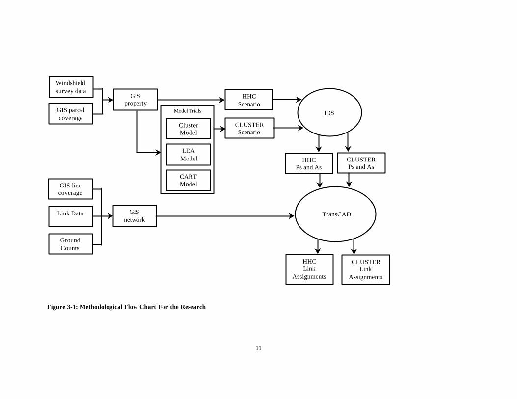
11

Model Trials

Windshieldsurvey data

ClusterModel

Figure 3-1: Methodological Flow Chart For the Research

GIS linecoverage

GISnetwork

file

Link Data

GIS parcelcoverage

GISproperty

tax

CLUSTERScenario

HHCScenario

IDS

HHCPs and As

CLUSTERPs and As

TransCAD

GroundCounts

HHCLink

Assignments

CLUSTERLink

Assignments

LDAModel

CARTModel

12

The two scenarios were run through IDS and the resulting Ps and As were processedthrough trip distribution and trip assignment using TranCAD following the sameprocedures outlined in Appendix H. Comparisons were then made between Ps resultingfrom the two methods. Productions were held constant while balancing Ps and As and sothe resulting As were likewise affected by the different methods used for categorizingdwelling units. Attractions were also compared between methods. Link assignmentsfrom each scenario can be compared to ground counts.

The overall general methodology for this project, as summarized above, was applied tothe case study Town of Pittsboro. The following chapter details the case study and thefindings.

13

4. HOUSEHOLD CONDITIONS BASED ON PROPERTY TAX

This project determined the relationships between household conditions based onwindshield surveys and property tax data. The analysis used year 2000 property tax dataand year 2000 windshield survey data for Pittsboro, NC.

The National Institute of Statistical Science (NISS) applied a statistical procedure calledK-means clustering to perform the analysis. NISS used the clustering method to classifypredictor variables in property tax data (acreage, land use value and improvement value)in an attempt to group the data into definable categories for trip rate assignment.

The methodology used by NISS for this portion of the project is outlined in the followingsection. Later sections detail each of the methodological steps and finally, results andconclusions round out the chapter.

Classification Methodology

Steps Involved:1. Choose a subjectively selected subset of variables in the property tax data that are

likely to be the most relevant in modeling HHCs. The variables for which dataare only partially available, i.e., variables for which data are largely missing, aredropped from the subset.

2. Compute the remaining set of variables as all real-valued so correlation can bedetermined between every pair of variables. The final set of variables used formodeling are selected to minimize the number of missing values in the finallyselected set and such that the correlation between the selected variables is as lowas possible.

3. Perform linear discriminant analysis and statistical measures (tests) to verify theadequacy of the model. The fitted model is used to obtain predictions on the dataset itself and the predictions are then compared with the windshield survey HHCsin order to check if the variables have any potential to serve as HHC predictors.

4. Use K-means clustering for classification. The number of clusters (K) for the datasegments has to be specified in advance. The procedure is tried with K =3,4,5,6,7,8,9,10,14 and visually inspected for each K. Finally K=7 is selected (i.e.divide the data into 7 clusters). Ideally, five clusters would be preferred to relateto the five traditional HHC categories.

Variable Selection

The primary focus of the analysis was to evaluate the capability of statistical models topredict HHC ratings using readily available property tax data as predictors. The propertytax data consisted of several fields such as: tax value of the land, tax value ofimprovements, acreage, perimeter of parcel, name of institutional or commercialestablishment, and so on. Such property tax data would replace currently assigned HHCsobtained by means of expensive, labor-intensive and subjective windshield surveys. The

14

general strategy fit a statistical classifier model, using training data for a set of parcels inPittsboro with HHC ratings, along with the property tax data available for the parcels.(Note that such training data would require subsequent windshield surveys in other citiesfor other models. Hence, some windshield surveys would always be necessary with thisapproach). Then the strategy evaluated the classifier model ability to reproduce theassigned HHC numbers in Pittsboro as well as ascertaining its generalizability to otherregions.

Preliminary exploration of the data revealed that:

• Several variables, e.g., area of the parcel and tax value, were highly correlated andwere essentially measures of the same latent feature of the parcel.

• Approximately 22.5% of the residential parcels were missing all or part of theyear 2000 property tax data.

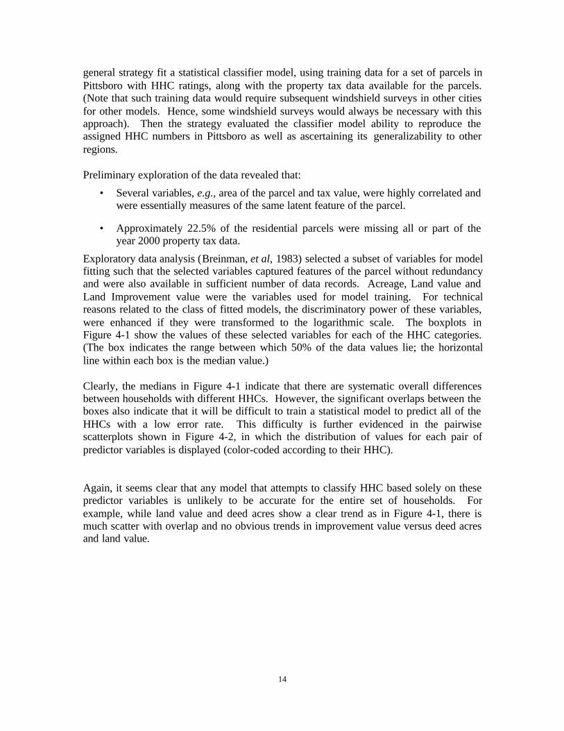
Exploratory data analysis (Breinman, et al, 1983) selected a subset of variables for modelfitting such that the selected variables captured features of the parcel without redundancyand were also available in sufficient number of data records. Acreage, Land value andLand Improvement value were the variables used for model training. For technicalreasons related to the class of fitted models, the discriminatory power of these variables,were enhanced if they were transformed to the logarithmic scale. The boxplots inFigure 4-1 show the values of these selected variables for each of the HHC categories.(The box indicates the range between which 50% of the data values lie; the horizontalline within each box is the median value.)

Clearly, the medians in Figure 4-1 indicate that there are systematic overall differencesbetween households with different HHCs. However, the significant overlaps between theboxes also indicate that it will be difficult to train a statistical model to predict all of theHHCs with a low error rate. This difficulty is further evidenced in the pairwisescatterplots shown in Figure 4-2, in which the distribution of values for each pair ofpredictor variables is displayed (color-coded according to their HHC).

Again, it seems clear that any model that attempts to classify HHC based solely on thesepredictor variables is unlikely to be accurate for the entire set of households. Forexample, while land value and deed acres show a clear trend as in Figure 4-1, there ismuch scatter with overlap and no obvious trends in improvement value versus deed acresand land value.

15

Figure 4-1: Distributions of the Predictors (log scale) for each HHC.

16

Figure 4-2: Pairwise Scatterplots of the Predictors.

Classification Techniques

To overcome the problems illustrated in Figures 4-1 and 4-2, NISS attemptedclassification using a number of techniques including linear regression, classificationtrees, linear discriminant analysis and k-means clustering. The findings are summarizedbelow.

Classification Tree

Tree-based modeling is widely used for classification problems. A tree model can bethought of as an optimal set of decision rules learned from a training data set that can beused to predict classes (HHC in the Pittsboro case) for a new set of predictor variables(the property tax data). For instance, a tree model fit to the Pittsboro data might yieldrules such as: “If (Acreage < a) then predict HHC = 1; Else (If Land_value < l thenHHC = 2; Else HHC = 4).” The set of rules can best be expressed in a logical treestructure. Several techniques exist for fitting tree-models [e.g., CART (InsightfulCorporation) and C4.5 (Quinlan, 1993)] that differ in the details of the rule learningalgorithm, as well as the model parameters that can be set to determine the complexity ofthe tree (rule set).

17

In this research, NISS used the tree model facilities built into the S-Plus (InsightfulCorporation). The tree results discussed below were unsatisfactory. Models thatadequately reproduced the windshield survey HHCs were too complex and would be veryunlikely to generalize well to other settings beyond Pittsboro; and conversely, the modelsthat might be more generalizable, were poor predictors.

Linear Discriminant Analysis

Classification based on discriminant functions can be justified using different lines ofreasoning (Ripley, 1996). In a situation where there are K classes to predict (k=5 HHCratings for IDS), the training data learn K linear functions of the predictor variables asfollows:

( ) Kcxaxaxaaxxxy ccccc ,...,2,1for ,, 3322110321 =+++=

Then the predicted HHC = c for a household if ( ) ( )321321 ,,,, xxxyxxxy jc > for .cj ≠

This classification approach fit the linear discriminant model in S-Plus using softwaredescribed in STATLIB. The resulting classifier was a little better than a tree-basedclassifier. NISS also attempted an extension of linear discriminants in which thediscriminant function was quadratic in the predictor variables which gives a more flexiblediscriminant function with potentially better predictive capability. However, thequadratic model was worse than the linear fits.

Linear discriminant analysis provided a reliable means of classifying the Pittsboro datainto HHC categories based on property tax information but sample HHC survey datamust be available for subsequent study areas. There are a number of advantages anddisadvantages to using this model.

Advantages:• Uses well known HHC classification scheme;• Will allow the use of traditionally prescribed trip rates for the five HHCs.

Disadvantages:• Due to the subjective nature of the HHCs being predicted, it is unlikely that the

Pittsboro model is transferable and the analysis has to be redone for each casecity. That is, windshield survey data would be needed for each region to train themodel. Therefore, the linear discriminant model does not eliminate windshieldsurveys and complicates the process.

Clustering of Households

The goal of the cluster analysis is to investigate if the property tax data itself can be usedto segment the households into categories related to trip rates. If such a categorization

18

can be done, NCDOT engineers can use the property tax profile as a surrogate for theHHCs and the engineers can assign trip-generation rates to the categories. It would thenbe possible to use the new categorization and circumvent the expensive and subjectiveHHC number assignments. The primary tools are statistical clustering methods (alsoknown as unsupervised learning methods). Methods such as k-means can partition thedata into clusters of households with similar property tax profiles.

This NISS approach used the simple, widely available technique of k-means clustering.In this method, the analyst first specified k, the number of clusters required. Then khouseholds were chosen at random as representatives for each of the clusters and eachhousehold was assigned to the cluster nearest to it. Next, the representatives of eachcluster were adjusted to the center (or “mean”) of the cluster. The process is thenrepeated with the new cluster representatives. Iterations continued until the clustersstabilized. The procedure was carried out in S-Plus. Several values of k were tried andthe appropriateness of resulting clusters were evaluated using data plots of the clusters aswell as the distribution of HHCs within each cluster. (Note that the HHCs windshieldsurvey would not typically be available if the clustering method is used in place of awindshield survey. Here it is used for additional guidance in the exploratoryinvestigation of the efficacy of the proposed technique). The clustering method finallysettled on clusters with k=7. (Actually this corresponds to effectively five clusters, sincetwo of the resulting seven clusters really represent outlying observations of Pittsboroproperties.)

There are a number of advantages and disadvantages associated with the clusteringmethod as well.

Advantages:• Clusters are based on natural breaks in the data and are not predicted based on a

model trained to simulate subjective HHCs;• There is no need to collect the windshield survey data at all.Disadvantages:• A new clustering analysis would have to be performed for each new town;• The clusters’ properties would have to be evaluated each time to determine

appropriate trip rates to assign to the clusters;• IDS or TransCAD trip generation models would have to be re-written to

accommodate cases where clusters are not the usual 5 clusters;• NCDOT staff would require training in new statistical software.

Discussion of Findings

In the models fit by the analysis, a cross-validation procedure is performed to balancecomplexity versus generalizability. This trade-off is to some extent due to the inherentsubjectivity of the HHC assignment. However, the primary reason for the limitedpredictive power of each of the classification tools is that the property tax data containonly part of the information used to assign HHCs. The surveyors in the field qualitativelyincorporate several other items of information such as number of vehicles on thepremises and neighborhood information in making a HHC assessment. This information

19

is not captured in the property tax data. However, the concept of replacing HHC surveysby property tax data should not be abandoned if the base year traffic model estimates arecomparable (as this research demonstrates).

A comparison of the various techniques (Table 4-1) show that although the k-meansclustering model may be more difficult to perform, it is the only model that is transferableand the only model that eliminates windshield survey.

Table 4-1: Comparison of Statistical Models Used to Classify Property Tax Data for Input into TripGeneration Model.

Model Data Requirements Ease of use TransferabilityCART HHCs and property tax data Advanced statistical techniques No

LDA HHCs and property tax data Advanced statistical techniques No

k-meansClustering

Property tax data Advanced statistical techniques Yes

Chapter Summary

The NCSU and NISS experiences with the classification and clustering analysis of theproperty-tax data suggest that statistical classifiers may be used for assigning HHCratings to dwelling units based on property-tax data. Unfortunately, as seen in Figure 4-1and Figure 4-2, the predictive accuracy of a model built solely from the property tax datais limited to the case study area. While it is possible to construct arbitrarily complexmodels that reproduce the HHCs for the case study training data exactly; it is unlikelythat they would generalize to other urban study areas.

The k-means clustering classifier method, for property taxes and HHCs, may be about asaccurate as windshield survey HHCs (as demonstrated in the subsequent case study). Asgeneralizability is of great concern, the clustering approach for bypassing HHCassignments is promising as it relies on the natural breaks in the data and does not linkclassifications to existing data as the learned models do. HHC classification, in the field,is based on factors other than housing condition and perceived worth, hence, augmentingthe property tax data with census data and car ownership data, may lead to moremeaningful clusters that are more readily interpretable for assigning trip-generation rates.

Although using natural breaks in the data to cluster properties into uniform property taxgroupings is promising, there are a number of drawbacks to this approach as well. First,a clustering will have to be performed for each city. This will involve statistical trainingfor the NCDOT engineers responsible for modeling each town. Second, it will requiretraining NCDOT engineers in a new way of assigning trip rates as clusters may notfollow the well known five category system used in the windshield survey method of datacollection. It may take an experienced engineer to determine the proper trip rates toassign to each cluster. As with IDS trip generation a “seed set” of trip rates could be usedto establish base year productions and attractions and resulting traffic assignments. Then

20

during the base year calibration and validation phase of the model, the trip rates could beadjusted if necessary to help match model traffic assignments to actual ground counts.This follows current NCDOT practice. Third, IDS or a modified TransCAD “IDS”would have to be re-written for more or less than five clusters.

Pittsboro demonstrates the clustering method to generate input data for IDS. Each of thesingle-family dwelling unit parcels is classified in the GIS database using the clusteringclassifier. The four-step travel forecasting process is then carried out based on the pre-calibrated base year windshield survey data (HHC scenario) and then the pre-calibratedcluster data (CLUSTER scenario). The outputs of these two scenarios are compared fortrip generation productions, attractions and assigned link volume to ground counts. Thecase study and results of the cluster analysis are described in the following chapter of thisreport.

21

5. THE PITTSBORO CASE STUDY

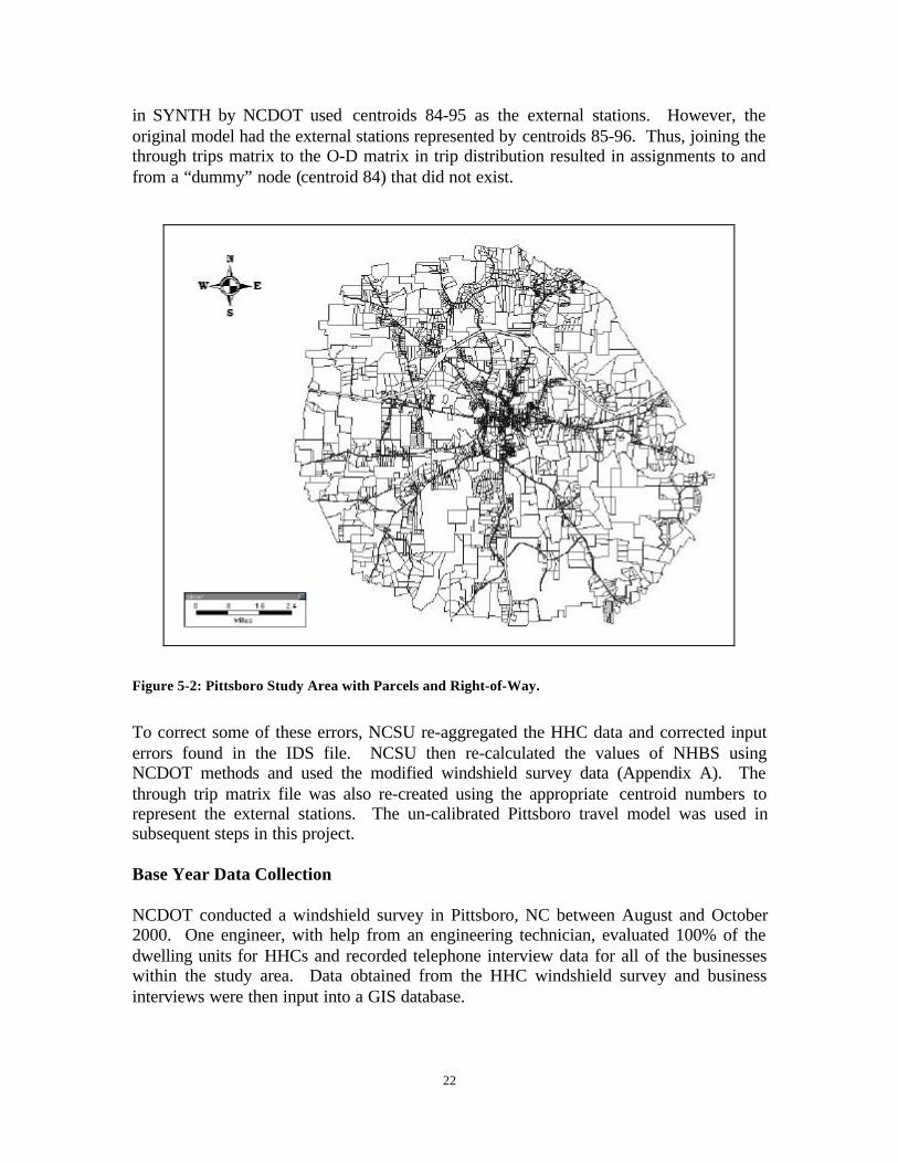
The Town of Pittsboro in Chatham County, North Carolina (Figure 5-1) is the case studyarea. This town was chosen because it is a current NCDOT small urban study and it hasavailable GIS property tax data. The study area includes all parcels within a five-mileradius of the town’s central traffic circle (Figure 5-2).

Figure 5-1: Vicinity Map of Pittsboro, NC (NTS) (Smithson, 2001)

Pittsboro Model Development

From August 2000 to May 2002, the NCDOT Statewide Planning Branch developed andcalibrated a base year transportation planning model for the Pittsboro area using HHCand IDS as the tool for trip generation and TransCAD for trip distribution andassignment. In September 2001, NCSU received an early version of the model. Beforethe model could be used in this research, NCSU had to make several adjustments.

The September 2001 NCDOT model for Pittsboro had several discrepancies. First, theIDS file contained non-reproducible values for non-home-based secondary (NHBS) trips.Second, several of the aggregated HHC numbers used in the IDS input file did notcorrespond to the numbers of households evaluated in the windshield survey and codedinto the parcel level database. Numbers were inverted. Third, in calibrating the model,NCDOT made direct adjustments to IDS output zone productions and attractions ratherthan adjustments to IDS input trip generation rates. Fourth, the through trips calculated

22

in SYNTH by NCDOT used centroids 84-95 as the external stations. However, theoriginal model had the external stations represented by centroids 85-96. Thus, joining thethrough trips matrix to the O-D matrix in trip distribution resulted in assignments to andfrom a “dummy” node (centroid 84) that did not exist.

Figure 5-2: Pittsboro Study Area with Parcels and Right-of-Way.

To correct some of these errors, NCSU re-aggregated the HHC data and corrected inputerrors found in the IDS file. NCSU then re-calculated the values of NHBS usingNCDOT methods and used the modified windshield survey data (Appendix A). Thethrough trip matrix file was also re-created using the appropriate centroid numbers torepresent the external stations. The un-calibrated Pittsboro travel model was used insubsequent steps in this project.

Base Year Data Collection

NCDOT conducted a windshield survey in Pittsboro, NC between August and October2000. One engineer, with help from an engineering technician, evaluated 100% of thedwelling units for HHCs and recorded telephone interview data for all of the businesseswithin the study area. Data obtained from the HHC windshield survey and businessinterviews were then input into a GIS database.

23

IDS requires each dwelling unit in each TAZ to be categorized as either excellent, aboveaverage, average, below average, or poor. Categorizing the dwelling units in each TAZ isaccomplished by the drive-by windshield survey. The drive-by windshield survey isconducted by driving by each parcel within the study area. If there is a buildingimprovement on the parcel, it is determined whether or not the use is residential.Residential uses include single detached housing (on-site construction and pre- fabhousing) and all multi-family units (duplex, triplex, apartments, dormitories, etc.). If thebuilding improvement on the parcel is residential, the parcel is then assigned a rating ofeither, excellent, above average, average, below average, or poor.

These ratings are measures of the trip-making propensity of each dwelling unit. It is upto the surveyor to determine the HHC rating for the dwelling unit. The surveyor assessesthe dwelling unit based on a number of physical features: the apparent age and size of thehouse, its appearance (well maintained or not), number of vehicles garaged, any signs ofchildren living in the house, and neighborhood appearance.

IDS uses the dwelling unit ratings to calculate productions by purpose including home-based work productions (HBWP), home-based other productions (HBOP) and non-home-based productions (NHBP). IDS uses the number of employers by employment categoryto calculate home-based work attractions (HBWA), home-based other attractions(HBOA) and non-home-based attractions (NHBA). Employment data is simultaneouslycollected during the drive-by windshield survey method. If the parcel being surveyedcontains a business, the name of the business is noted. The local phone book is used tolook up the telephone number of the business. NCDOT contacts each business bytelephone and asks the nature of the business, number of employees and number ofcommercial vehicles operating out of that business. The type of business is needed inorder to assign that business the appropriate Standard Industrial Classification (SIC) code(Table 5-1). The assigned SIC code is then used to categorize the business into one of thefive employment categories required for IDS. The five IDS employment categories areindustrial, retail, highway retail, office, and service.

During the August to October 2000 windshield survey, over 4000 parcels were surveyedresulting in the rating of 2385 households (Figure 5-3) and the categorization of 2,664employees by their employment type.

Table 5-1: Employment Categories by SIC Code (Smithson, 2001).

IDS EmploymentCategories SIC CodesIndustry 1-49Retail 55,58HwyRetail 50-54,56,57,59Office 60-67, 91-97Service 70-76, 78-89, 99

24

Pittsboro GIS Database

Four primary databases containing socio-economic data were used for this project:• 1993 Property Tax Data (Chatham County, GIS Department);• 2000 Property Tax Data (Chatham County, GIS Department);• Parcel Database (developed by NCSU);• TAZ Database (developed by NCDOT).

Figure 5-3: Household Ratings by Parcel.

Parcel Level Database

Chatham County provided the 1993 Property Tax Database. This database contains thegeographic delineation and information or attributes pertaining to each parcel within thestudy area. This database provides the foundation for development of the ParcelDatabase used in TransCAD. The Chatham County database also contains manyattributes not necessary for the model. These fields were deleted to reduce the size of thedatabase. Examples of fields dropped are owner’s name, owner’s address, 1993 landvalue, 1993 improvement value and certain fields used for reference by Chatham County.Fields or attributes that were kept include parcel identification numbers (PINs), acreage,land tax value, improvement tax value, and land use. Chatham County property taxexaminers re-evaluated land parcels in 2000 for property tax purposes. These were stored

25

in a database and merged to the 1993 Chatham County Property Tax Database. Only taxvalues obtained in the 2000 tax assessment were used for this project.

The Parcel Database was created by adding fields for household condition ratings andassigned TAZs to the edited Chatham County database described in the previousparagraph. Additional fields are described below. Appendix B provides a sample of theParcel database.Area Area of ParcelPerimeter Perimeter of ParcelPIN Parcel Identification NumberLand_FMV Tax value of land (year 2000)IMPR _FM Tax value of Improvement (year 2000)DEED_A Acreage of parcelLU_Parcel Land use or type of propertyTAZ_00 Assigned TAZHHC_00 2000 Household condition RatingHHC_95 1995 Household condition RatingTAZ_95 TAZ number for Regional ModelMTAZ Census TAZ number used in Regional Model

Aggregated TAZ Level Database

The TAZ Database is then created after completion of the Parcel Database describedabove. Essentially, each parcel within the Parcel Database with the same TAZassignment are merged into one polygon. The single-family dwelling units per householdcondition rating are aggregated at the zonal level and entered into the database.Employment data is then added to each TAZ. As with the household condition ratings,employment data is entered by type for each TAZ. The TAZ database attribute fields aredescribed below. Appendix C gives a sample of the TAZ database.ID Record ID (produced by TransCADPITTTAZ_00 Pittsboro TAZ numberINDEMP Number of employees in Industrial employmentRETEMP Number of employees in Retail employmentHWYEMP Number of employees in Highway Retail employmentOFFEMP Number of employees in Office employmentTOTEMP Total number of employees in TAZHH1 Number of households with a POOR rating in TAZHH2 Number of households with a BELOW AVERAGE rating in TAZHH3 Number of households with an AVERAGE rating in TAZHH4 Number of households with an ABOVE AVERAGE rating in

TAZHH5 Number of households with an EXCELLENT rating in TAZTOTHH Total number of households in TAZ

26

Network Database

The network database was supplied in a line coverage from NCDOT. The NCDOT linefiles are not sufficient for travel demand modeling purposes. NCDOT line files onlycontain the coordinates of the endpoints that define each link, the length of the link, andstreet name. The NCDOT street database (shown in Appendix D) is thus expanded toinclude speed, time, link-type, and capacity. Speed limits and roadway cross-sectionswere gathered from field surveys in Pittsboro. Link travel time is a function of lengthand speed and the “time” column in the street database is filled with the followingformula: length/speed*60. The result is travel time in minutes for each link. The “link-type” column contains link codes based on link classifications or categories (i.e. centroidconnectors). Link capacity depends upon a number of physical features of a roadwaysuch as shoulder widths, lane widths, number of lanes in each direction, and speed limits.

Internal Data Summary

The NCDOT uses an in-house program called IDS for the trip generation phase of thefour step planning process, discussed in the Introduction of this report. The inputs intoIDS are trip rates, dwelling unit data aggregated to the TAZ level, NHBS trips andaggregated employment data based on SICs for each TAZ.

Two different TAZ database files were created and used as input into IDS (Appendix F)to estimate the balanced productions and attractions. The data files differ only in the dataused as ratings for the dwelling units and the calculated NHBS trips. All group dwellingunit data, employment data, external station data and trip rates (Table 5-2) are the samefor the two scenarios.

Table 5-2: IDS Daily Vehicle Trip Generation Rates by Household Condition Used in Pittsboro Study(Smithson, 2001).

HouseholdCondition

Excellent AboveAverage

Average BelowAverage

Poor

Trip Rate 12.0 10.0 8.0 7.0 5.0

The scenarios are as defined below:1. HHC: The data model used year 2000 windshield survey data for the household

condition ratings 1 through 5, aggregated at the TAZ level. This input file variedfrom the NCDOT base year model in the number of NHBS trips and the modificationof aggregated HHC numbers for some TAZs that did not correspond to the numberscoded into the parcel database file. This adjustment corrected the coding errorsdiscussed earlier.

2. CLUSTER: This data model used NISS predicted clusters aggregated to the TAZlevel. The two outlying clusters that contained two parcels each were added into thepreceding clusters. There were a number of parcels that could not be evaluated usingthe NISS clustering model. Of the 2386 dwelling units evaluated by the NCDOT inthe windshield survey, NCSU researchers were not able to classify 536 of them, usingthe NISS classifier. The three main reasons why a property was not classified are:

27

• More than one dwelling unit on a parcel;• Missing land value from property tax record; and• No property tax data available for the parcel.

Those parcels that contained a single-family dwelling unit and had all of the propertytax data were evaluated using the NISS classifier. For those properties that had morethan one dwelling unit on it, the additional dwelling units were assigned the samecluster value as that predicted for the parcel using the NISS classifier. For the parcelswith missing property tax data, the dwelling units were evaluated based on thedistribution of dwelling units among clusters in that TAZ. For example, a TAZ withtwenty missing dwelling units and with the following distribution:

• 20% in cluster A• 50% in cluster B• 30% in cluster D

the twenty missing dwelling units were be assigned as follows: ten of the missingdwelling units are assigned to cluster B, four to cluster A and six to cluster D.

Each of the two models (Appendix E and Appendix F) were run through IDS. Theproductions for the two methods were compared to one another using the statisticalprocedures outlined in the following section. Attractions were compared in a similarmanner. Trip distribution and assignment were carried out using the same proceduresused by the NCDOT in the base year analysis of Pittsboro (Appendix G).

Statistical Comparisons

The un-calibrated productions from the HHC scenario IDS output file were compared tothe IDS productions from the CLUSTER scenario. Comparisons were made at the zonallevel for each trip purpose. Attractions were compared in a similar manner. Thecomparisons used un-calibrated productions and attractions because the un-calibratedvalues are input for trip distribution and subsequently for traffic assignment. Only whenestimated link volumes are available for validation against base year ground counts aretrip generation model trip rates adjusted and Ps and As re-calculated and the model rerununtil estimated link volumes approximate ground counts.

Assuming the zonal productions from two different methods are a paired sample, thedifferences between trips produced by each zone are calculated. The resultingdifferences for each zone become a single sample of differences about which inferencescan be made. Differences in productions for each trip purpose and differences inattractions for each trip purpose were calculated individually. The null hypothesis is thatthere is no difference between productions or attractions resulting from the input HHCand CLUSTER data. Therefore, the mean of the sample of differences is compared to anexpected mean (µD) of zero using a one sample t-test (Equation 5-1).

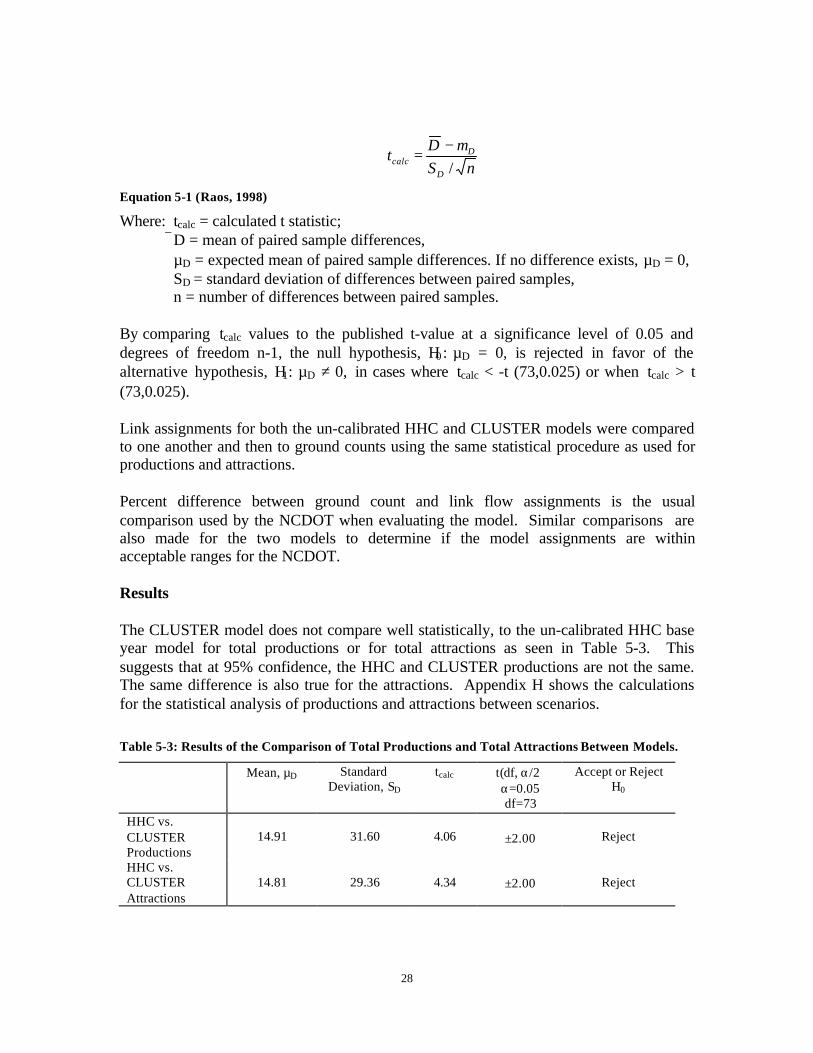
28

Equation 5-1 (Raos, 1998)

Where: tcalc = calculated t statistic; D = mean of paired sample differences,

µD = expected mean of paired sample differences. If no difference exists, µD = 0,SD = standard deviation of differences between paired samples,n = number of differences between paired samples.

By comparing tcalc values to the published t-value at a significance level of 0.05 anddegrees of freedom n-1, the null hypothesis, H0 : µD = 0, is rejected in favor of thealternative hypothesis, H1: µD ≠ 0, in cases where tcalc < -t (73,0.025) or when tcalc > t(73,0.025).

Link assignments for both the un-calibrated HHC and CLUSTER models were comparedto one another and then to ground counts using the same statistical procedure as used forproductions and attractions.

Percent difference between ground count and link flow assignments is the usualcomparison used by the NCDOT when evaluating the model. Similar comparisons arealso made for the two models to determine if the model assignments are withinacceptable ranges for the NCDOT.

Results

The CLUSTER model does not compare well statistically, to the un-calibrated HHC baseyear model for total productions or for total attractions as seen in Table 5-3. Thissuggests that at 95% confidence, the HHC and CLUSTER productions are not the same.The same difference is also true for the attractions. Appendix H shows the calculationsfor the statistical analysis of productions and attractions between scenarios.

Table 5-3: Results of the Comparison of Total Productions and Total Attractions Between Models.

Mean, µD StandardDeviation, SD

tcalc t(df, α/2)α=0.05df=73

Accept or RejectH0

HHC vs.CLUSTERProductions

14.91 31.60 4.06 ±2.00 Reject

HHC vs.CLUSTERAttractions

14.81 29.36 4.34 ±2.00 Reject

nSD

tD

Dcalc /

µ−=

29

The models are also compared at the trip purpose level. Statistical comparisons of theHHC and CLUSTER model are summarized in Table 5-4 and calculations are found inAppendix I. Differences at a 95% confidence level are noted between productions for theHHC and CLUSTER models for all of the trip purposes. The same is noted fordifferences in attractions between models.

The mean difference between productions for the HBW and NHB trip purposes are quitelow and are seen in Table 5-4. The mean difference for the HBW is 3.69 productions perTAZ between the two models and 2.76 for the NHB productions. In practical applicationof the trip generation model these differences are negligible.

Table 5-5 shows the entire set of productions by model and TAZ as well as thedifferences between models by trip purpose. Differences range between -26 to 42productions for the HBW and 0 to 25 for NBH productions (CLUSTER – HHC). For 13of the 74 TAZs HHC productions are higher than CLUSTER HBW productions; for 8TAZs there is no difference between model HBW productions and for 53 TAZs, theCLUSTER model yields higher HBW productions than the HHC model. For half of theTAZs, the CLUSTER model and HHC model yield the same results for NHBproductions. For the remaining 37 TAZs, the CLUSTER model over estimates theproductions. HBO differences show a little more variability and a higher mean differenceof productions between models, with differences range from -58 to 96.

The external trips are not influenced by the household condition ratings of parcels withinthe planning area or by the clusters and are not in the IDS file. Productions andattractions for external trips thus remain the same regardless of scenario. They are notcompared in this analysis.

Table 5-4: Results of the Comparison Between the HHC Model and the CLUSTER Model by TripPurpose.

Trip Purpose Mean, µD StandardDeviation, SD

Tcalc t(df, α/2) Accept or Reject H0

Home-based WorkProductions

3.69 8.94 3.55 ±2.00 Reject

Home-based OtherProductions 8.46 20.33 3.58 ±2.00 Reject

Non-Home-BasedProductions 2.76 5.68 4.18 ±2.00 Reject

Home-based WorkAttractions

3.66 9.11 3.45 ±2.00 Reject

Home-based OtherAttractions 8.36 17.85 4.03 ±2.00 Reject

Non-Home-BasedAttractions 2.79 5.79 4.15 ±2.00 Reject

30

Table 5-5: Production Results and Differences Between the HHC Model and the CLUSTER Modelby Trip Purpose.

HHC CLUSTER CLUSTER-HHC

TAZ HBW HBO NHB HBW HBO NHB HBW HBO NHB1 33 76 19 46 105 20 13 29 12 24 54 7 24 55 7 0 1 03 71 161 106 77 176 107 6 15 14 0 0 0 0 0 0 0 0 05 55 125 27 71 162 28 16 37 16 141 320 133 154 350 136 13 30 37 95 217 968 106 242 984 11 25 168 138 313 925 180 409 941 42 96 169 2 4 51 1 3 52 -1 -1 110 37 84 7 41 93 7 4 9 011 44 100 12 51 115 12 7 15 012 31 71 7 33 76 7 2 5 013 95 217 192 91 207 196 -4 -10 414 139 317 788 150 341 801 11 24 1315 62 140 513 69 158 522 7 18 916 90 206 27 110 251 28 20 45 117 81 184 780 95 217 794 14 33 1418 13 30 12 11 25 12 -2 -5 019 55 126 651 49 111 662 -6 -15 1120 225 511 659 254 577 670 29 66 1121 64 145 82 64 147 84 0 2 222 49 112 157 69 157 160 20 45 323 48 109 317 45 103 323 -3 -6 624 44 99 748 49 111 761 5 12 1325 24 56 784 27 61 798 3 5 1426 41 94 369 48 110 375 7 16 627 2 6 0 3 7 0 1 1 028 86 195 66 92 209 67 6 14 129 4 10 0 4 10 0 0 0 030 85 193 91 90 205 92 5 12 131 8 19 513 8 19 522 0 0 932 35 79 670 39 89 682 4 10 1233 28 63 1066 34 77 1084 6 14 1834 61 139 1457 76 173 1482 15 34 2535 22 51 686 19 44 698 -3 -7 1236 34 78 43 40 90 44 6 12 137 10 24 0 12 27 0 2 3 038 7 15 0 9 21 0 2 6 039 31 70 7 35 79 7 4 9 040 53 121 12 51 116 12 -2 -5 041 15 34 4 20 46 4 5 12 042 36 81 7 42 96 7 6 15 043 31 71 7 30 68 7 -1 -3 0

31

44 12 27 659 13 30 670 1 3 1145 25 58 329 26 58 335 1 0 646 78 177 561 97 221 571 19 44 1047 19 43 4 16 37 4 -3 -6 048 50 115 12 45 103 12 -5 -12 049 0 0 46 0 0 48 0 0 250 26 59 7 31 71 7 5 12 051 6 13 0 7 15 0 1 2 052 147 334 43 174 395 44 27 61 153 13 31 4 15 35 4 2 4 054 6 13 392 6 13 398 0 0 655 7 15 0 8 19 0 1 4 056 17 39 4 19 44 4 2 5 057 23 53 4 26 59 4 3 6 058 22 51 4 21 47 4 -1 -4 059 0 0 0 0 0 0 0 0 060 23 53 7 33 76 7 10 23 061 36 82 7 42 96 7 6 14 062 77 175 16 51 117 17 -26 -58 163 13 30 4 15 35 4 2 5 064 35 79 7 45 102 7 10 23 065 47 107 32 57 129 32 10 22 066 26 60 32 31 71 32 5 11 067 35 80 98 41 94 100 6 14 268 26 59 4 27 62 4 1 3 069 14 31 4 16 37 4 2 6 070 8 18 0 9 21 0 1 3 071 16 37 12 19 43 12 3 6 072 16 37 4 18 41 4 2 4 073 20 46 4 24 55 4 4 9 074 57 129 16 52 119 17 -5 -10 1

While the statistical tests directly compare the estimates of Ps and As by the HHC andCLUSTER methods, the ultimate validation of the base year model for the study area ishow well it duplicates ground counts. Thus, a test can be performed for ground countsversus estimated traffic flow. If that overall model test yields positive results,discrepancies in Ps and As (Tables 5-3, 5-4 and 5-5) may be downplayed.

The traditional way in which the NCDOT compares ground counts to estimated flows isin keeping with the J. Robbins (1978) estimates of accuracy of travel demand forecastingparameters. Table 5-6 summarizes the results of the comparison of flows from thedifferent scenarios to the ground counts. Table 5-6 shows that the flows estimated usingthe CLUSTER method are quite similar to those obtained using the HHC method.

The mean percent difference between ground counts and the two scenario flows arewithin ± 29%. The CLUSTER model results in a lower mean percent difference betweenground counts and flows than does the HHC model. The CLUSTER model also shows a

HHC CLUSTER CLUSTER-HHCTAZ HBW HBO NHB HBW HBO NHB HBW HBO NHB

32

“Ground Count: Model Flows” ratio slightly closer to unity than the HHC model. Thenumber of links within acceptable percent error range is the same for both scenarios(Table 5-6). The acceptable percent difference between ground count and estimated linkvolumes depends on the functional class of the roadway and can be as large as 100% forcertain local roadways.

Table 5-6: Results of the Comparison Between Link Assignments for the HHC Unadjusted,CLUSTER and Ground Counts.

Mean,µD

StandardDeviation,

SD

tcalc t(df,α/2)

Mean %Differencein Flows

Number ofLinks’ Flows

WithinAcceptable

Error*

GroundCount:ModelFlowsRatio

Ground CountsVs. CLUSTER 910.0 1981.1 3.44 ±2.00 25.37 14/56 0.85

Ground CountsVs. HHC 830.2 1922.3 3.23 ±2.00 28.81 14/56 0.84

* Robbins, J. (1978). Mathematical Models-the Error of Our Ways. Traffic Engineering & Control , Vol.18(1).

Figure 5-5 shows the flows that result from using the CLUSTER method for determininginput into the IDS model used for trip generation in the four step planning process.Figure 5-6 shows the flows derived from using the HHCs from windshield surveys in theIDS model. Note that the loaded networks are very similar for the two methods.

Figure 5-5: CLUSTER method daily flow.

33

Figure 5-6: HHC method daily flow.

Discussion

The analysis of productions and attractions reveals that the CLUSTER model does notcompare well to the HHC model for overall productions or overall attractions at the 95%confidence level. When looking at the models in detail, it appears that the CLUSTERmodel has a lower tcalc for HBWP, HBWA and HBOP than for the other trip purposes.The highest mean differences between scenario productions and attractions are found forthe HBO trip purpose. HBO trips also show the greatest variations in differences for bothproductions and attractions. The CLUSTER model results in Ps, As and estimated flowsthat are less than those produced using the windshield survey data. The two methods oftrip generation data input result in Ps and As that are statistically different betweenmodels at the 95% confidence level.

The mean difference between productions for the HBW and NHB trip purposes are quitelow. The mean difference for the HBW is 3.69 productions per TAZ between the twomodels and 2.76 for the NHB productions. In practical application of the trip generationmodel these differences are negligible. The same trend is documented for the attractions.

Both methods result in traffic flows that are statistically different from ground counts atthe 95% confidence level. A comparison of the un-calibrated HHC and the CLUSTERmodels shows a mean percent difference between ground counts and link assignmentsgreater than 25% which is well above the acceptable limits for calibrated NCDOTmodels. Mean percent differences between ground counts and flows for the HHC model

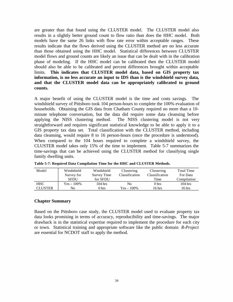
34

are greater than that found using the CLUSTER model. The CLUSTER model alsoresults in a slightly better ground count to flow ratio than does the HHC model. Bothmodels have the same 26 links with flow rate error within acceptable ranges. Theseresults indicate that the flows derived using the CLUSTER method are no less accuratethan those obtained using the HHC model. Statistical differences between CLUSTERmodel flows and ground counts are likely an issue that can be dealt with in the calibrationphase of modeling. If the HHC model can be calibrated then the CLUSTER modelshould also be able to be calibrated and percent differences brought within acceptablelimits. This indicates that CLUSTER model data, based on GIS property taxinformation, is no less accurate an input to IDS than is the windshield survey data,and that the CLUSTER model data can be appropriately calibrated to groundcounts.

A major benefit of using the CLUSTER model is the time and costs savings. Thewindshield survey of Pittsboro took 104 person-hours to complete the 100% evaluation ofhouseholds. Obtaining the GIS data from Chatham County required no more than a 10-minute telephone conversation, but the data did require some data cleansing beforeapplying the NISS clustering method. The NISS clustering model is not verystraightforward and requires significant statistical knowledge to be able to apply it to aGIS property tax data set. Total classification with the CLUSTER method, includingdata cleansing, would require 8 to 16 person-hours (once the procedure is understood).When compared to the 104 hours required to complete a windshield survey, theCLUSTER model takes only 15% of the time to implement. Table 5-7 summarizes thetime-savings that can be achieved using the CLUSTER method for classifying singlefamily dwelling units.Table 5-7: Required Data Compilation Time for the HHC and CLUSTER Methods.

Model WindshieldSurvey for

SFDU

WindshieldSurvey Time

for SFDU

ClusteringClassification

ClusteringClassification

Time

Total TimeFor Data

CompilationHHC Yes – 100% 104 hrs No 0 hrs 104 hrsCLUSTER No 0 hrs Yes – 100% 16 hrs 16 hrs

Chapter Summary

Based on the Pittsboro case study, the CLUSTER model used to evaluate property taxdata looks promising in terms of accuracy, reproducibility and time-savings. The majordrawback is in the statistical expertise required to implement the procedure for each cityor town. Statistical training and appropriate software like the public domain R-Projectare essential for NCDOT staff to apply the method.

35

6. CONCLUSIONS AND RECOMMENDATIONS

Statistical Classification

This project developed a method for grouping and classifying GIS based property taxdata into categories for use in the IDS trip generation model. NISS determined that deedacres, improvement value and land value were the three best predictors of householdcondition in the Pittsboro case study. Using these three variables, NISS carefullyreviewed the various statistical techniques (LDA, CART and k-means clustering)available for this type of categorization. NISS found that models that adequatelyreproduced the windshield survey HHCs were too complex and would be very unlikely togeneralize well to other settings beyond Pittsboro; and conversely, the models that mightbe more generalizable, were poor predictors. NISS selected the k-means clusteringmethod for the reasons outlined below. NISS used the statistical package called S-Plus,however, NCDOT should consider the public domain package R-Project for clustering.

The k-means method groups properties into clusters based on natural breaks in the data.Clusters are assigned to properties based on the statistical similarity between the propertytax characteristics of the land parcels. Parcels with similar characteristics are groupedinto the same cluster. The clusters are used instead of HHC ratings for single familydwelling units for the purpose of trip generation. The advantages of this method are that:

• Properties can be assigned cluster values without the subjective evaluation of theHHC surveyor. Once the clusters are established, appropriate trip rates can beapplied.

• Clusters do not have to follow the 5 HHC categories of IDS.• Clusters are not based on HHC ratings as is the case with the CART and LDA

approaches.• Clustering does not require any windshield survey to be done.

The disadvantage to the k-means clustering approach is that a new clustering would haveto be performed for each city. The NCDOT would have to train some of their employeesto carry out the analysis.

Using HHC as a means of predicting the trip making propensity of the people in adwelling unit is time consuming and costly. NISS’s suggested use of property tax dataclusters is promising in that it allows the natural breaks in the data to be recognized andused for classification. Replicating a subjective HHC rating system based on windshieldsurveys is not be the best approach to classifying households.

One of the challenges of the statistical analysis is to balance complexity versusgeneralizability of the clustering model. In doing so, the predictive power of theclassification tool is often limited. In this case, the limitation was to some extent due tothe inherent subjectivity of the HHC assignment. However, the primary reason for the

36

limited predictive power of each of the classification tools is that the property tax datacontain only part of the information used to assign HHCs. The surveyors in the fieldincorporate several other items of information such as number of vehicles on thepremises and neighborhood information in making a HHC assessment. This extrainformation is not adequately captured in the property tax data and could help to increasethe predictive power of the k-mean clustering model.

GIS Property Tax Database

In order to use property GIS based property tax data in a meaningful way for tripgeneration purposes, it is essential to design a database that incorporates all of thenecessary attributes. NISS discovered a number of parcels that were missing part or allof the property tax data required (deed acres, improvement value and land value) toclassify the parcels using either of the statistical procedure identified. These missing data(536 out of 2386 parcels did not have complete data) could be one reason that the tripgeneration results from the CLUSTER model did not compare well to the results of theHHC model.

Data compilation would be facilitated if there were statewide GIS standards for codingparcel information (PINs, etc.). A standard format is essential for joining informationfrom external databases into the GIS parcel layer.

Maintaining a parcel level database file for each study area is essential. It allowsplanners to adjust TAZs boundaries as conditions change. TAZ level database files canbe built in TransCAD based on the TAZ field in the parcel level database.

Recommended fields to include in a parcel level database that is to be used for clusteringare as follows:Area Area of ParcelPerimeter Perimeter of ParcelPIN Parcel Identification NumberLand_FMV Tax value of land (base year)IMPR _FM Tax value of Improvement (base year)DEED_A Acreage of parcelLU_Parcel Land use or type of propertyTAZ Assigned TAZMTAZ Census TAZ number used in Regional ModelINDEMP Number of employees in Industrial employmentRETEMP Number of employees in Retail employmentHWYEMP Number of employees in Highway Retail employmentOFFEMP Number of employees in Office employmentCLUSTER1 Number of households in the first cluster on parcelCLUSTER2 Number of households second cluster on parcelCLUSTER3 Number of households in third cluster on parcelCLUSTER4 Number of households in fourth cluster on parcel

37

CLUSTER5 Number of households in fifth cluster on parcel (incorporate additionalfields for study areas with more than 5 clusters)

The Pittsboro Case Study

This project applies a statistical classification method to the case study Town ofPittsboro. Both standard HHC input data and CLUSTER data were used in the traveldemand model for Pittsboro.

The two methods result in traffic flows that are statistically different from ground countsat the 95% confidence level. A comparison of the un-calibrated HHC and the CLUSTERmodels shows a mean percent difference between ground counts and link assignmentsgreater than 25% which is above the acceptable limits for calibrated NCDOT models.Mean percent difference between ground count and flows for the HHC model is greaterthan that found using the CLUSTER model. The CLUSTER model also results in aslightly better ground count to flow ratio than does the HHC model. Both models havethe same 26 links with flow error within acceptable ranges. These results indicate thatthe flows derived using the CLUSTER method are no less accurate than those obtainedusing the HHC model. Statistical differences between CLUSTER model flows andground counts are likely an issue that can be dealt with in the calibration phase ofmodeling. If the HHC model can be calibrated then the CLUSTER model should also beable to be calibrated and percent differences brought within acceptable limits. Thisindicates that CLUSTER model data, based on GIS property tax information, is no lessaccurate an input to IDS than is the windshield survey data. However, the meandifference between productions for the HBW and NHB trip purposes are quite low. Themean difference for the HBW is 3.69 productions per TAZ between the two models and2.76 for the NHB productions. In practical application of the trip generation model thesedifferences are negligible. The same trend is documented for the attractions.

The benefits of using the CLUSTER model is the time-savings associated with its use.The windshield survey of Pittsboro took 104 person-hours to complete the 100%evaluation of households. Obtaining the GIS data from Chatham County required nomore than a 10-minute telephone conversation but did require some data cleansing effortsbefore applying the NISS clustering method. The NISS clustering model is not verystraightforward and requires statistical knowledge to be able to apply it to a GIS propertytax data set. Total classification with the CLUSTER method, including data cleansing,would require 8-16 person-hours (once the procedure is understood). When compared tothe 104 hours required to complete a windshield survey, the CLUSTER model takes only15% of the time to implement.

The CLUSTER model used to evaluate property tax data looks promising in terms oftime-savings. The major drawback is in the statistical training required to implement theprocedure for each city or town. Another case study should be performed to test thetransferability of the clustering approach.

38

Summary Recommendations

The specific recommendations for NCDOT, resulting from this project follow:1. Test the use of GIS based property tax data in another North Carolina city.2. Enrich the property data with other data like vehicle ownership and census data to

enhance the predictive power of the k-means clustering classification tool.3. Conduct the comparisons of productions, attractions and link volumes on calibrated

trip generation models, as well as un-calibrated models.4. Obtain software and tutorial guides so that NCDOT staff can become familiar with k-

means clustering. R-Project may be a source of information.5. Contact county tax departments and discuss data format and data items that are

needed for travel forecasting and compare them to developing NCDOT standards.6. Establish a statewide database definition for all parcel level GIS coverages and

encourage state and municipal organizations to adopt it.

Recommended Methodology for Use of Clustering

In order to use the clustering method in travel demand modeling there are several steps tocarry out. The following is a general recommended methodology for using cluster data inplace of windshield survey input data for trip generation.

1. Obtain countywide GIS cadastral coverage from the county GIS department.2. Determine the extent of the study area and clip the county cadastral layer to include

only parcels within that boundary.3. Obtain current property tax data including land value, improvement value and deed

acres (if not already included in cadastral coverage) and adjust to current year values.4. Determine which records in the database file represent single family dwelling units.

Create a selection set containing the single family dwelling units and convert that to anew database file. Make adjustments for group quarters.

5. Take the new database file and determine which of the records contain all of therequired property tax data (land value, deed acres and improvement value). Eliminatethose that are missing data.

6. Using statistical software, apply the k-means clustering procedure to the remainingdatabase records. After several iterations, the k-means clustering method will assigncluster numbers to each record that is in the data set.

7. Join the data set, complete with cluster assignments, back into the original study areaGIS database file.

8. Aggregate data based on TAZ boundaries.9. Prepare the IDS input file containing aggregated cluster assignments.10. Proceed with trip generation, trip distribution, mode split and network assignment

following the traditional procedures used by NCDOT.

39

7. REFERENCES

Breinman, L., Friedman, J.H., Olshen, R.A., and C.J. Stone (1983). CART: Classificationand Regression Trees, Wadsworth, Belmont, CA.

Caliper Corporation (2000). TransCAD, Transportation GIS Software. Newton, MA,http://www. Caliper.com/

CAMPO (1999). CAMPO Newsletter. Raleigh, NC http://www.raleigh-nc.org/campo/Newsletfw99.htm.

FHWA (1998a), Transportation Case Studies in GIS Case Study 2: Portland Metro,Oregon – GIS database for Urban Transportation Planning, Report # FHWA-PD-98-065 No. 2.

FHWA (1998b), Transportation Case Studies in GIS Case Study 3: NCDOT: Use of GISto Support Environmental Analysis During System Planning, Report # FHWA-PD-98-065, No. 3.

Goulias, K.G. and R. Kitamura (1992). Travel Demand Forecasting with DynamicMicrosimulation. Transportation Research Record 1347.

He, Y. (1999). EUTSTIS: A Comprehensive Database System to Support TransportationStudies in and MPO. ITE Journal, Vol: 69 (3).

Hyashi, Y. and Y. Tomita (1989). A Micro-Analytic Residential Mobility Model forAssessing the Effects of Transportation Improvement. Transport Policy,Management & Technology Towards 2001: Selected Proceedings of the FifthWorld Conference on Transport Research, Volume 4.

Insightful Corporation (last accessed 2001). S-PLUS Product Familyhttp://www.insightful.com.

Los Alamos National Laboratory (1999). Transims Overview, Vol: 0. Los Alamos, NM.

NCDOT (1999). Internal Data Summary (IDS), NCDOT notes for data input and output.Received September 1999.

NCDOT (1997). NCDOT Travel Forecasting Training Manual, Prepared for the NCDOTStatewide Planning Branch, Raleigh, NC.

NuStats International (1995). Triangle Travel Behavior Survey. Prepared for the TriangleTransit Authority, Raleigh, NC.

40

Parsons Transportation Group (2000). Wake County Automated Data System: TravelBehavior Analysis. Prepared for the Capital Area Planning Organization.

Quinlan, J.R. (1993), C4.5: Programs for Machine Learning, Morgan Kaufmann, SanMateo, CA.

Ripley, B.D (1996). Pattern Recognition and Neural Networks, Cambridge UniversityPress.

Robbins, J. (1978). Mathematical Models- the Error of Our Ways. Traffic Engineering &Control, Vol. 18(1).

Rouphail, N.M; Frey, H.C.; Unal, A.; Dalton, R., and A. Karr (2000). ITS Integration ofReal-Time Emissions and Traffic Management Systems. IDEA Program ResearchReport, ITS-44. Prepared for the IDEA Program, Transportation Research BoardNational Research Council.

THE R PROJECT FOR STATISTICAL COMPUTING (last accessed 2001),http://www.r-project.org.

Shinebein, P.J. (1999). Developing a Geographic Information System Travel DemandForecasting Model for Las Vegas. . ITE Journal, Volume 69 (2).

Smithson, W.D. (2001). A Travel Demand Model For Pittsboro, North Carolina: A CaseStudy Using TransCAD, A GIS Based Software. Masters Project Submitted to theUniversity of North Carolina, Chapel Hill, NC.

STATLIB (last accessed 2001), http://lib.stat.cmu.edu.

Stone, J.R., et.al. (2000). Assessing the Feasibility of TRANSIMS in North Carolina.FHWA/NCDOT/2000-05.

Tukey, J.W. (1977). Exploratory Data Analysis, Addison-Wesley, Reading, MA.

Urban Analysis Group (1995). Tranplan User Manual, Hayward, CA,http://www.minutp.com/.

Venables, W. and B. Ripley (1997). Modern applied statistics using S-PLUS, (2nd Ed.),Springer, New York, NY.

VISUAL INSIGHTS, ADVIZOR, http://www.visualinsights.com.

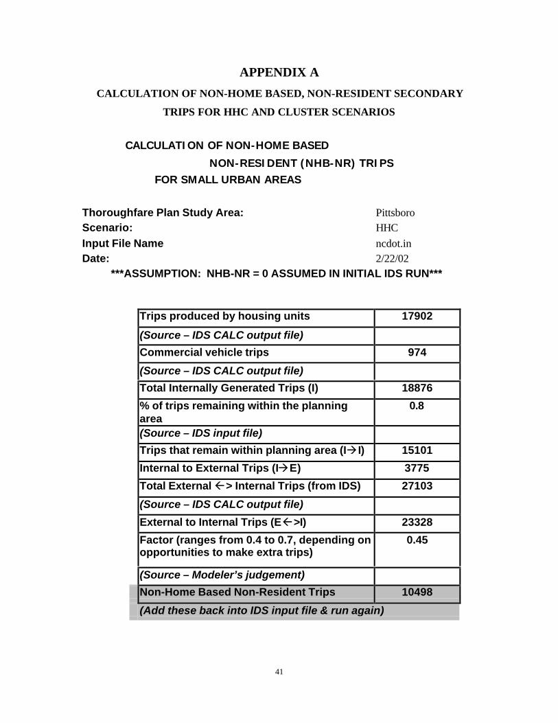
41

APPENDIX A

CALCULATION OF NON-HOME BASED, NON-RESIDENT SECONDARY

TRIPS FOR HHC AND CLUSTER SCENARIOS

CALCULATION OF NON-HOME BASED

NON-RESIDENT (NHB-NR) TRIPSFOR SMALL URBAN AREAS

Thoroughfare Plan Study Area: PittsboroScenario: HHCInput File Name ncdot.inDate: 2/22/02

***ASSUMPTION: NHB-NR = 0 ASSUMED IN INITIAL IDS RUN***

Trips produced by housing units 17902

(Source – IDS CALC output file)

Commercial vehicle trips 974

(Source – IDS CALC output file)

Total Internally Generated Trips (I) 18876

% of trips remaining within the planningarea

0.8

(Source – IDS input file)

Trips that remain within planning area (Ià I) 15101

Internal to External Trips (IàE) 3775

Total External ß> Internal Trips (from IDS) 27103

(Source – IDS CALC output file)

External to Internal Trips (Eß>I) 23328

Factor (ranges from 0.4 to 0.7, depending onopportunities to make extra trips)

0.45

(Source – Modeler’s judgement)

Non-Home Based Non-Resident Trips 10498

(Add these back into IDS input file & run again)

42

CALCULATION OF NON-HOME BASEDNON-RESIDENT (NHB-NR) TRIPS

FOR SMALL URBAN AREAS

Thoroughfare Plan Study Area: PittsboroScenario: CLUSTERInput File Name NCSU.inDate: 2/22/02

***ASSUMPTION: NHB-NR = 0 ASSUMED IN INITIAL IDS RUN***

Trips produced by housing units 19918

(Source – IDS CALC output file)

Commercial vehicle trips 974

(Source – IDS CALC output file)

Total Internally Generated Trips (I) 20892

% of trips remaining within the planningarea

0.8

(Source – IDS input file)

Trips that remain within planning area (Ià I) 16714

Internal to External Trips (IàE) 4178

Total External ß> Internal Trips (from IDS) 27103

(Source – IDS CALC output file)

External to Internal Trips (Eß>I) 22925

Factor (ranges from 0.4 to 0.7, depending onopportunities to make extra trips)

0.45

(Source – Modeler’s judgement)

Non-Home Based Non-Resident Trips 10316

(Add these back into IDS input file & run again)

43

APPENDIX B

SAMPLE PARCEL DATABASE FILE

ID PIN LAND_FMV IMPR_FMV DEED_ACRES LU_PARCEL PITTTAZ_00 HHC_00 MU_00 NEW_TAZ CLUSTER1417 9742-44-5184.000 128000 133434 18.000 Single Family

Residential74 4 0 74 1

1413 9742-24-7627.000 35050 127900 4.010 Single FamilyResidential

74 4 0 74 3

1252 9742-26-4081.000 210996 273673 44.610 Single FamilyResidential

74 4 0 74 1

1362 9742-15-7147.000 37500 133034 2.190 Single FamilyResidential

74 4 0 74 3

1341 9742-15-5543.000 33750 156684 2.000 Single FamilyResidential

74 4 0 74 3

1513 9742-53-0501.000 21750 185298 1.500 Single FamilyResidential

74 4 0 74 1

1242 9742-05-3903.000 189920 35109 33.480 Single FamilyResidential

74 3 0 74 7

1131 9742-47-3808.000 20505 102642 1.101 Single FamilyResidential

74 3 0 74 3

1357 9742-15-4361.000 33750 127306 2.120 Single FamilyResidential

74 3 0 74 3

1331 9742-15-5628.000 33750 142934 2.000 Single FamilyResidential

74 3 0 74 3

1313 9742-15-4885.000 33750 142465 2.000 Single FamilyResidential

74 3 0 74 3

1296 9742-16-4073.000 33750 131758 2.000 Single FamilyResidential

74 3 0 74 3

1277 9742-16-4241.000 33750 147714 2.000 Single FamilyResidential

74 3 0 74 3

1251 9742-16-4309.000 33750 144853 2.000 Single FamilyResidential

74 3 0 74 3

1249 9742-16-2571.000 33750 143888 2.040 Single FamilyResidential

74 3 0 74 3

1246 9742-16-0581.000 33750 156609 2.000 Single FamilyResidential

74 3 0 74 3

1244 9742-06-8496.000 33750 123496 2.000 Single FamilyResidential

74 3 0 74 3

44

APPENDIX C

SAMPLE TAZ DATABASE FILE

ID AREA PITTTAZ_00

INDEMP

RETEMP

HWYRET

OFFEMP

SERVEMP

TOTEMP

HH1 HH2 HH3 HH4 HH5 TOTHH TAZ_00 CAR PUP VAN BUS TRK BEDS

1 0.002664 0 0 0 0 0 0 02 0.354618 1 0 0 0 0 1 1 1 23 3 0 0 27 13 1.209644 2 2 0 0 0 0 2 1 3 7 4 1 16 24 2.218294 3 3 11 0 0 0 14 3 20 21 8 0 52 35 0.351996 4 0 0 0 0 0 0 0 0 0 0 0 0 0

6 1.426570 5 0 0 0 0 1 1 10 27 4 4 0 45 57 2.255241 6 0 1 0 0 9 10 5 42 41 14 1 103 68 2.221431 7 7 1 0 0 95 103 3 31 26 8 1 69 79 2.688641 8 2 28 0 0 67 97 63 38 24 1 0 126 8 1510 0.750785 9 17 0 0 4 0 21 0 0 0 1 0 1 9 811 2.201250 10 0 0 0 0 0 0 0 12 12 3 0 27 1012 0.690984 11 0 0 0 0 0 0 3 17 12 2 0 34 1113 1.089796 12 3 0 0 0 0 3 5 6 7 3 2 23 12 4

14 0.455912 13 0 0 0 0 15 15 0 14 43 10 0 67 1315 1.090354 14 19 2 31 3 0 55 18 31 53 6 0 108 1416 0.786351 15 0 0 4 1 36 41 4 24 19 1 0 48 1517 0.707835 16 0 0 0 0 0 0 8 22 40 0 0 70 1618 0.834608 17 37 6 4 0 56 103 2 54 9 0 0 65 17 119 3.364412 18 1 0 0 0 1 2 0 3 3 3 0 9 1820 0.339099 19 4 6 3 0 82 95 0 9 15 12 1 37 19 1

21 0.094756 20 0 0 0 0 149 149 0 169 11 0 0 180 20 6 4 3122 0.052521 21 0 0 2 0 0 2 5 12 19 9 1 46 2123 0.114315 22 1 3 0 0 12 16 19 17 7 1 0 44 22 3 2 124 0.053863 23 12 1 4 0 16 33 0 17 13 5 0 35 23 1 225 0.042332 24 6 29 5 37 99 176 5 15 11 3 0 34 24 2 5 126 0.037396 25 3 37 32 20 24 116 0 7 10 1 0 18 25 1 3 4 20

45

APPENDIX D

SAMPLE NETWORK DATABASE FILE

ID LENGTH DIR LINK_TYPE CAPACITY_ SPEED_ TIME_ FNODE_ TNODE_ STREET ADT_01 TRUCK375 1.69 0 1 9000.00 40.00 2.54

399 0.20 0 1 9000.00 40.00 0.30 11200.0037 0.21 0 1 9000.00 40.00 0.32 1200.0091 0.68 0 1 9000.00 40.00 1.02 184 145 N US 15-501

112 0.64 0 1 9000.00 40.00 0.96191 0.19 0 1 9000.00 40.00 0.28 304 287

228 0.19 0 1 9000.00 40.00 0.29 326 325330 0.14 0 1 9000.00 40.00 0.21 2625.00

363 0.56 0 1 9000.00 40.00 0.8458 0.25 0 1 9000.00 40.00 0.38 112 106 SILK HOPE G 1050.00

59 0.78 0 1 9000.00 40.00 1.17132 0.42 0 1 9000.00 40.00 0.64 251 246 W US 64 HWY

136 1.00 0 1 9000.00 40.00 1.50 256 246 OLD SILER C272 0.09 0 1 9000.00 40.00 0.14 348 360 9200.00

422 0.37 0 1 9000.00 40.00 0.55277 0.22 0 1 9000.00 40.00 0.33 344 363

436 1.51 0 1 9000.00 40.00 2.27284 0.35 0 1 9000.00 40.00 0.53 345 372 OLD GOLDSTO415 0.34 0 1 9000.00 40.00 0.51

301 0.21 0 1 9000.00 40.00 0.32312 0.20 0 1 9000.00 40.00 0.31

313 0.20 0 1 9000.00 40.00 0.29 350.00410 0.23 0 1 9000.00 40.00 0.35 9250.00

350 0.23 0 1 9000.00 40.00 0.35 1500.00358 0.24 0 1 9000.00 40.00 0.36 455 458 PITTSBORO-G

398 0.04 0 1 9000.00 40.00 0.06

46

APPENDIX E

IDS INPUT FILE FOR HHC METHOD IDS HHC METHOD 2001 PRELIM WITH NHBS = 10498 96 ZONES (74 ZONES+22 STATIONS) 96 48600 10498 80 22 50 28 250 250 250 250 250 1200 1000 800 700 500 670 67 670 670 100 100 100 100 100 030 010 200 840 260 250 010 020 200 840 260 250 010

050 200 840 260 250 010 1 0 0 3 23 1 0 0 0 2 1 4 7 3 1 0 0 0 3 0 8 21 20 3 0 0 0 4 0 0 0 0 0 0 0 0 5 0 4 4 27 10 0 0 0 6 1 14 41 42 5 0 0 0

7 1 9 26 31 3 0 0 0 8 0 1 24 38 63 0 0 0 9 0 1 0 0 0 0 8 0 10 0 3 12 12 0 0 0 0 11 0 2 12 17 3 0 0 0 12 2 3 7 6 5 0 4 0 13 0 10 43 14 0 0 0 0 14 0 6 53 31 18 0 0 0 15 0 1 19 24 4 0 0 0 16 0 0 40 22 8 0 0 0 17 0 0 9 54 2 0 1 0 18 0 3 3 3 0 0 0 0 19 1 12 15 9 0 0 1 0 20 0 0 11 170 0 0 10 0 21 1 9 19 12 5 0 0 0 22 0 1 7 17 19 0 6 0 23 0 5 13 17 0 0 3 0 24 0 3 11 15 5 0 8 0 25 0 1 10 7 0 0 8 0 26 0 0 12 17 4 0 5 0 27 0 0 0 2 0 0 0 0 28 0 8 27 25 3 0 1 0 29 0 0 3 0 0 0 0 0 30 0 0 36 27 1 0 2 0 31 0 1 2 3 0 0 13 0 32 0 0 12 13 2 0 4 0 33 0 1 7 10 4 0 8 0 34 0 0 13 31 5 0 6 0 35 0 0 1 17 0 0 10 0 36 0 1 12 12 1 0 0 0 37 0 0 3 5 0 0 0 0 38 0 1 0 4 0 0 0 0 39 0 0 14 9 0 0 0 0 40 5 11 7 11 0 0 0 0 41 0 0 2 9 1 0 0 0 42 0 2 11 12 2 0 0 0 43 0 3 13 6 0 0 0 0 44 0 0 5 4 0 0 6 0

47

45 0 0 11 8 0 0 0 0 46 0 0 21 35 6 0 8 0 47 0 2 11 0 0 0 0 0 48 0 14 13 6 0 0 0 0 49 0 0 0 0 0 0 2 0 50 0 0 10 9 1 0 0 0 51 0 0 3 1 0 0 0 0 52 0 4 47 57 4 0 0 0 53 0 0 6 4 0 0 30 0 54 0 1 2 1 0 0 0 0 55 0 0 2 3 0 0 0 0 56 0 0 6 7 0 0 0 0 57 0 2 8 7 0 0 0 0 58 2 7 3 0 2 0 0 0 59 0 0 0 0 0 0 0 0 60 0 0 6 7 7 0 0 0 61 0 4 13 8 1 0 0 0 62 6 27 12 0 0 0 0 0 63 0 1 3 5 1 0 0 0 64 0 2 11 9 5 0 0 0 65 0 2 15 18 0 0 0 0 66 0 1 13 5 0 0 1 0 67 0 1 15 10 0 0 0 0 68 0 0 14 5 0 0 0 0 69 0 1 5 4 0 0 0 0 70 0 0 3 3 0 0 0 0 71 0 2 6 2 2 0 0 0 72 0 4 3 4 0 0 0 0 73 0 0 10 5 0 0 0 0 74 0 7 22 11 0 0 0 0 75 76 77 78 79 80 81 82 83 84 85 86 87 88 89 90 91 92 93 94 95 96 1 0 0 0 0 1 2 2 0 0 0 0 3 3 11 0 0 0 4 0 0 0 0 0 5 0 0 0 0 1 6 0 1 0 0 9 7 7 1 0 0 95 8 2 28 0 0 67 9 17 0 0 4 0 10 0 0 0 0 0 11 0 0 0 0 0

48

12 3 0 0 0 0 13 0 0 0 2 15 14 10 2 21 3 0 15 0 0 4 1 36 16 0 0 0 0 0 17 37 6 4 0 56 18 1 0 0 0 1 19 4 6 3 0 50 20 0 0 0 0 60 21 0 0 2 0 0 22 1 3 0 0 12 23 12 1 4 0 16 24 6 15 5 20 25 25 3 15 13 10 13 26 0 0 1 28 4 27 0 0 0 0 0 28 5 5 0 0 0 29 0 0 0 0 0 30 0 0 0 0 7 31 0 0 0 35 16 32 5 8 9 15 15 33 10 7 15 30 20 34 0 20 18 15 55 35 0 0 10 0 36 36 0 2 0 0 2 37 0 0 0 0 0 38 0 0 0 0 0 39 0 0 0 0 0 40 0 0 0 0 0 41 0 0 0 0 0 42 0 0 0 0 0 43 0 0 0 0 0 44 0 0 0 0 67 45 0 0 0 25 7 46 0 0 0 0 55 47 0 0 0 0 0 48 0 0 0 0 0 49 0 0 0 0 5 50 0 0 0 0 0 51 0 0 0 0 0 52 0 0 0 0 0 53 0 0 0 0 0 54 500 0 0 0 0 55 0 0 0 0 0 56 0 0 0 0 0 57 0 0 0 0 0 58 0 0 0 0 0 59 0 0 0 0 0 60 0 0 0 0 0 61 0 0 0 0 0 62 0 0 0 0 0 63 3 0 0 0 0 64 0 0 0 0 0 65 0 0 0 0 2 66 8 0 0 0 2 67 0 0 0 0 9 68 0 0 0 0 0 69 0 0 0 0 0 70 0 0 0 0 0 71 0 0 0 0 1 72 0 0 0 0 0 73 0 0 0 0 0 74 0 0 0 0 0

49

75 76 77 78 79 80 81 82 83 84 85 4576 86 6268 87 614 88 1777 89 911 90 4413 91 222 92 1321 93 1422 94 134 95 3979 96 1466

50

APPENDIX F

IDS INPUT FILE FOR CLUSTER METHOD IDS CLUSTER METHOD 2001 WITH NHBS = 10316 96 ZONES (74 ZONES+22 STATIONS) 96 48600 10316 80 22 50 28 250 250 250 250 250 1200 1000 800 700 500 670 67 670 670 100 100 100 100 100 030 010 200 840 260 250 010 020 200 840 260 250 010

050 200 840 260 250 010 1 0 23 4 0 0 0 0 0 2 2 5 5 1 3 0 0 0 3 0 18 23 10 1 0 0 0 4 0 0 0 0 0 0 0 0 5 0 25 14 6 0 0 0 0 6 4 33 41 22 3 0 0 0 7 2 33 18 11 6 0 0 0 8 4 28 38 55 1 0 0 0 9 0 0 1 0 0 0 8 0 10 1 9 13 3 1 0 0 0 11 1 11 14 7 1 0 0 0 12 0 9 6 6 2 0 4 0 13 0 10 25 28 4 0 0 0 14 0 23 50 23 12 0 0 0 15 0 18 12 14 4 0 0 0 16 1 39 15 15 0 0 0 0 17 4 8 46 6 1 0 1 0 18 0 2 1 2 4 0 0 0 19 0 6 9 17 5 0 1 0 20 0 59 76 7 39 0 10 0 21 0 6 28 11 1 0 0 0 22 1 20 18 5 0 0 6 0 23 0 0 18 14 3 0 3 0 24 0 7 20 6 1 0 8 0 25 0 5 11 2 0 0 8 0 26 0 6 25 2 0 0 5 0 27 0 1 1 0 0 0 0 0 28 0 17 33 12 1 0 1 0 29 0 1 0 2 0 0 0 0 30 0 9 38 17 0 0 2 0 31 0 0 4 2 0 0 13 0 32 0 5 18 4 0 0 4 0 33 0 11 4 7 0 0 8 0 34 0 24 18 6 1 0 6 0 35 2 0 2 0 14 0 10 0 36 3 5 13 5 0 0 0 0 37 0 2 6 0 0 0 0 0 38 1 4 0 0 0 0 0 0 39 3 6 7 5 2 0 0 0 40 5 7 8 13 1 0 0 0 41 0 9 3 0 0 0 0 0 42 2 10 10 5 0 0 0 0 43 0 5 3 13 1 0 0 0 44 1 0 7 1 0 0 6 0 45 0 1 9 9 0 0 0 0

51

46 0 29 32 1 0 0 8 0 47 0 0 0 13 0 0 0 0 48 0 3 16 14 0 0 0 0 49 0 0 0 0 0 0 2 0 50 3 6 8 1 2 0 0 0 51 0 3 1 0 0 0 0 0 52 1 52 43 15 1 0 0 0 53 1 4 2 2 1 0 30 0 54 0 0 3 1 0 0 0 0 55 0 3 2 0 0 0 0 0 56 0 7 2 2 2 0 0 0 57 0 6 9 2 0 0 0 0 58 3 5 0 1 5 0 0 0 59 0 0 0 0 0 0 0 0 60 0 15 4 1 0 0 0 0 61 1 18 2 3 2 0 0 0 62 0 2 1 27 15 0 0 0 63 1 2 6 1 0 0 0 0 64 0 20 5 2 0 0 0 0 65 2 17 15 1 0 0 0 0 66 0 13 6 0 0 0 1 0 67 0 15 8 3 0 0 0 0 68 0 3 13 3 0 0 0 0 69 1 5 2 2 0 0 0 0 70 0 2 4 0 0 0 0 0 71 0 7 3 1 1 0 0 0 72 0 8 2 1 0 0 0 0 73 4 2 7 2 0 0 0 0 74 2 5 3 24 6 0 0 0 75 76 77 78 79 80 81 82 83 84 85 86 87 88 89 90 91 92 93 94 95 96 1 0 0 0 0 1 2 2 0 0 0 0 3 3 11 0 0 0 4 0 0 0 0 0 5 0 0 0 0 1 6 0 1 0 0 9 7 7 1 0 0 95 8 2 28 0 0 67 9 17 0 0 4 0 10 0 0 0 0 0 11 0 0 0 0 0 12 3 0 0 0 0

52

13 0 0 0 2 15 14 10 2 21 3 0 15 0 0 4 1 36 16 0 0 0 0 0 17 37 6 4 0 56 18 1 0 0 0 1 19 4 6 3 0 50 20 0 0 0 0 60 21 0 0 2 0 0 22 1 3 0 0 12 23 12 1 4 0 16 24 6 15 5 20 25 25 3 15 13 10 13 26 0 0 1 28 4 27 0 0 0 0 0 28 5 5 0 0 0 29 0 0 0 0 0 30 0 0 0 0 7 31 0 0 0 35 16 32 5 8 9 15 15 33 10 7 15 30 20 34 0 20 18 15 55 35 0 0 10 0 36 36 0 2 0 0 2 37 0 0 0 0 0 38 0 0 0 0 0 39 0 0 0 0 0 40 0 0 0 0 0 41 0 0 0 0 0 42 0 0 0 0 0 43 0 0 0 0 0 44 0 0 0 0 67 45 0 0 0 25 7 46 0 0 0 0 55 47 0 0 0 0 0 48 0 0 0 0 0 49 0 0 0 0 5 50 0 0 0 0 0 51 0 0 0 0 0 52 0 0 0 0 0 53 0 0 0 0 0 54 500 0 0 0 0 55 0 0 0 0 0 56 0 0 0 0 0 57 0 0 0 0 0 58 0 0 0 0 0 59 0 0 0 0 0 60 0 0 0 0 0 61 0 0 0 0 0 62 0 0 0 0 0 63 3 0 0 0 0 64 0 0 0 0 0 65 0 0 0 0 2 66 8 0 0 0 2 67 0 0 0 0 9 68 0 0 0 0 0 69 0 0 0 0 0 70 0 0 0 0 0 71 0 0 0 0 1 72 0 0 0 0 0 73 0 0 0 0 0 74 0 0 0 0 0 75

53

76 77 78 79 80 81 82 83 84 85 4576 86 6268 87 614 88 1777 89 911 90 4413 91 222 92 1321 93 1422 94 134 95 3979 96 1466

54

APPENDIX G

NCDOT BASE YEAR PROCEDURE FOR

PITTSBORO (SMITHSON, 2001)

Trip Distribution

Trip distribution is the second step in the four-step modeling process. Trip distribution iswhere the productions and attractions developed for each TAZ are “distributed”throughout the planning area using a gravity model. The required inputs to tripdistribution are a balanced production/attraction table, an impedance matrix, and afriction factor matrix for each trip purpose. The balanced production/attraction table wascreated during trip generation. The impedance matrix, used to represent the amount ofdifficulty of traveling between any pair of zones, was developed from the Pittsboro streetnetwork files. Once an impedance matrix is developed, the friction factor matrix iscreated. The friction factor matrix contains the friction factor for travel between eachpair of TAZ’s.

Pittsboro Network Development

Developing an impedance matrix requires a transportation network. The Pittsboro linefiles were “clipped” from the Chatham County street database.

The final step in network development is attaching the Pittsboro TAZ’s to the Pittsboronetwork. To connect an area (a TAZ) to a line file (Pittsboro network) in TransCAD,click the Tools drop down menu, click Map Editing, and then the Connect feature.TransCAD will prompt the user for the geographic area file and the line layer file the userwould like to connect. TransCAD places a “centroid” in each TAZ and creates a newlink to connect the centroid to the closest link or node on the network.

Connecting TAZ’s to Street Network

The new links are called centroid connectors and are assigned the value of “2” in thelink-type column in the line layer database. The centroids TransCAD placed in eachTAZ are also added to the line layer database and assigned a record ID matching the TAZnumber. This feature allows the user to recognize points that represent a TAZ from pointsdefining the shape of a link.

Creating the Impedance Matrix

Link travel times were used to develop the impedance between TAZ pairs. InTransCAD, impedances are stored in a zone-to-zone matrix. An impedance matrix isgenerated in TransCAD by applying the Multiple Shortest Path function to a network.The procedure generates shortest paths between multiple origins and multipledestinations and creates a matrix file containing the impedance of traversing each path.

55

In TransCAD, click the Network/Paths drop down menu then click Multiple Paths.TransCAD will prompt the user for the network file and to select the endpointsrepresenting the TAZ’s. The output is an impedance matrix for each pair of zones basedon travel time.

Developing Friction Factors

Friction factors are a required input in the gravity model. Friction factors are inverselyproportional to impedance.

The equation is as follows: f(cij) = a(cij)^-b * e^-c(cij), where a>0, c>= 0

The gamma function requires user specification of the parameters to be used in themodel. Travel Estimation Techniques for Urban Planning (NCHRP365, 1995) suggeststhat the gamma function be used with the following parameters (Table 1):

Table 1: Recommended Gamma Function Parameters

Trip Purpose A b C

HBW 28507 0.02 0.123HBO 139173 1.285 0.094NHB 219113 1.332 0.01

To create friction factors in TransCAD click Planning from the drop down menu. SelectTrip Distribution then select Synthetic Friction Factors. TransCAD opens the frictionfactor matrix dialogue box. In this box the user specifies the impedance function (gammafunction), and types in the function parameters to be used for each trip purpose. The usermust also specify the file location of the impedance matrix created and discussed in theabove section. The TransCAD output is a set of friction factor matrices for each trippurpose specified.

Applying the Gravity Model

Applying the gravity model in TransCAD is a simple procedure. The TAZ geographicfile must be the active window in TransCAD. Choose Planning from the drop downmenu, select Trip Distribution, then select Gravity Evaluation. TransCAD displays thegravity evaluation dialogue box. The user specifies the file containing the productionsand attractions (the TAZ geographic file) and the location of the friction factor matricesfor each trip purpose. TransCAD generates P-A (production-attraction) flow matrices foreach trip purpose. The trip purpose matrices are then summed to create a total P-A flowmatrix of all trip purposes. To sum matrices in TransCAD, choose Matrix from the dropdown menu and click Quick Sum.

56

Thru-trips and Converting P-A Matrix to O-D Matrix

The final steps in trip distribution are adding the thru-trips calculated in SYNTH to theQuick Sum matrix described above. The Quick Sum matrix only includes the HBW,HBO, NHB, and Ext-Int trips. The balanced thru-trip matrix developed in SYNTH isconverted to a matrix file in TransCAD. The thru-trip matrix is then combined with theQuick Sum matrix for use in traffic assignment, the final step in the travel demandmodeling process. To convert the thru-trip matrix to a TransCAD matrix file chooseMatrix from the drop down menu and select Import. TransCAD makes the conversion tothe appropriate format. To join the thru-trip matrix to the Quick Sum matrix, simplychoose Matrix and select Combine. The thru-trips are now added to the P-A flow matrixgenerated during gravity evaluation.

Prior to traffic assignment, TransCAD requires the P-A flow matrix to be converted to anOD (origin-destination) matrix. The active window must be the total P-A flow matrix.Choose Planning and select PAtoOD. The result is an OD matrix for trip purposes foreach TAZ. At this point, all the inputs required for traffic assignment have beendeveloped.

Mode Split

Mode split is the third step in the four-step travel demand model. This step has beenintentionally left out of the Pittsboro study.

Traffic Assignment

Traffic assignment models are used to estimate the flow of traffic on a network. Thetraffic assignment model used for the Pittsboro study is an All-or-Nothing assignment. Insmall towns similar to Pittsboro, NCDOT uses an All-or-Nothing assignment whencongestion may not be a factor in route choice.

Required inputs for traffic assignment include an O-D matrix and a network. To performthe traffic assignment for the Pittsboro model in TransCAD, the O-D matrix discussedabove and the modified Pittsboro network from the NCDOT GIS Unit were used. InTransCAD, the Pittsboro network was made the active window. Choose Planning fromthe drop down menu and select Traffic Assignment. TransCAD opens the trafficassignment dialogue box. The traffic assignment method (All-or-Nothing) and thedesired O-D matrix must be selected. No changes were made to the default fieldssettings. TransCAD stores the assigned traffic volumes to a link-flow table and joins thetable to the network file.

57

APPENDIX H

STATISTICAL COMPARISON OF PRODUCTIONS AND ATTRACTION: CALCULATIONS

Total Productions Comparison

Mean t-calc t(n-1,α/2) Reject/Accept df=73, α=0.0514.91 4.06 2.00 Reject Ho: µd−µo=0

Standard Dev31.60

HHC CLUSTER

TAZ HBW HBO NHB EXT Total HHC TAZ HBW HBO NHB EXT TotalCLUSTER

D=CLUSTER-HHC D2

1 33 76 19 0 128 1 46 105 20 0 171 43 1849

2 24 54 7 0 85 2 24 55 7 0 86 1 1

3 71 161 106 0 338 3 77 176 107 0 360 22 4844 0 0 0 0 0 4 0 0 0 0 0 0 0

5 55 125 27 0 207 5 71 162 28 0 261 54 29166 141 320 133 0 594 6 154 350 136 0 640 46 2116

7 95 217 968 0 1280 7 106 242 984 0 1332 52 27048 138 313 925 0 1376 8 180 409 941 0 1530 154 23716

9 2 4 51 0 57 9 1 3 52 0 56 -1 110 37 84 7 0 128 10 41 93 7 0 141 13 169

11 44 100 12 0 156 11 51 115 12 0 178 22 48412 31 71 7 0 109 12 33 76 7 0 116 7 49

13 95 217 192 0 504 13 91 207 196 0 494 -10 10014 139 317 788 0 1244 14 150 341 801 0 1292 48 2304

15 62 140 513 0 715 15 69 158 522 0 749 34 115616 90 206 27 0 323 16 110 251 28 0 389 66 4356

58

17 81 184 780 0 1045 17 95 217 794 0 1106 61 372118 13 30 12 0 55 18 11 25 12 0 48 -7 49

19 55 126 651 0 832 19 49 111 662 0 822 -10 10020 225 511 659 0 1395 20 254 577 670 0 1501 106 11236

21 64 145 82 0 291 21 64 147 84 0 295 4 1622 49 112 157 0 318 22 69 157 160 0 386 68 4624

23 48 109 317 0 474 23 45 103 323 0 471 -3 924 44 99 748 0 891 24 49 111 761 0 921 30 900

25 24 56 784 0 864 25 27 61 798 0 886 22 48426 41 94 369 0 504 26 48 110 375 0 533 29 84127 2 6 0 0 8 27 3 7 0 0 10 2 4

28 86 195 66 0 347 28 92 209 67 0 368 21 44129 4 10 0 0 14 29 4 10 0 0 14 0 0

30 85 193 91 0 369 30 90 205 92 0 387 18 32431 8 19 513 0 540 31 8 19 522 0 549 9 81

32 35 79 670 0 784 32 39 89 682 0 810 26 67633 28 63 1066 0 1157 33 34 77 1084 0 1195 38 1444

34 61 139 1457 0 1657 34 76 173 1482 0 1731 74 547635 22 51 686 0 759 35 19 44 698 0 761 2 4

36 34 78 43 0 155 36 40 90 44 0 174 19 36137 10 24 0 0 34 37 12 27 0 0 39 5 25

38 7 15 0 0 22 38 9 21 0 0 30 8 6439 31 70 7 0 108 39 35 79 7 0 121 13 169

40 53 121 12 0 186 40 51 116 12 0 179 -7 4941 15 34 4 0 53 41 20 46 4 0 70 17 28942 36 81 7 0 124 42 42 96 7 0 145 21 441

43 31 71 7 0 109 43 30 68 7 0 105 -4 1644 12 27 659 0 698 44 13 30 670 0 713 15 225

45 25 58 329 0 412 45 26 58 335 0 419 7 4946 78 177 561 0 816 46 97 221 571 0 889 73 5329

47 19 43 4 0 66 47 16 37 4 0 57 -9 81

59

48 50 115 12 0 177 48 45 103 12 0 160 -17 28949 0 0 46 0 46 49 0 0 48 0 48 2 4

50 26 59 7 0 92 50 31 71 7 0 109 17 28951 6 13 0 0 19 51 7 15 0 0 22 3 9

52 147 334 43 0 524 52 174 395 44 0 613 89 792153 13 31 4 0 48 53 15 35 4 0 54 6 36

54 6 13 392 0 411 54 6 13 398 0 417 6 3655 7 15 0 0 22 55 8 19 0 0 27 5 25

56 17 39 4 0 60 56 19 44 4 0 67 7 4957 23 53 4 0 80 57 26 59 4 0 89 9 8158 22 51 4 0 77 58 21 47 4 0 72 -5 25

59 0 0 0 0 0 59 0 0 0 0 0 0 060 23 53 7 0 83 60 33 76 7 0 116 33 1089

61 36 82 7 0 125 61 42 96 7 0 145 20 40062 77 175 16 0 268 62 51 117 17 0 185 -83 6889

63 13 30 4 0 47 63 15 35 4 0 54 7 4964 35 79 7 0 121 64 45 102 7 0 154 33 1089

65 47 107 32 0 186 65 57 129 32 0 218 32 102466 26 60 32 0 118 66 31 71 32 0 134 16 256

67 35 80 98 0 213 67 41 94 100 0 235 22 48468 26 59 4 0 89 68 27 62 4 0 93 4 16

69 14 31 4 0 49 69 16 37 4 0 57 8 6470 8 18 0 0 26 70 9 21 0 0 30 4 16

71 16 37 12 0 65 71 19 43 12 0 74 9 8172 16 37 4 0 57 72 18 41 4 0 63 6 3673 20 46 4 0 70 73 24 55 4 0 83 13 169

74 57 129 16 0 202 74 52 119 17 0 188 -14 19675 0 0 0 0 0 75 0 0 0 0 0 0 0

76 0 0 0 0 0 76 0 0 0 0 0 0 077 0 0 0 0 0 77 0 0 0 0 0 0 0

78 0 0 0 0 0 78 0 0 0 0 0 0 0

60

79 0 0 0 0 0 79 0 0 0 0 0 0 080 0 0 0 0 0 80 0 0 0 0 0 0 0

81 0 0 0 0 0 81 0 0 0 0 0 0 082 0 0 0 0 0 82 0 0 0 0 0 0 0

83 0 0 0 0 0 83 0 0 0 0 0 0 084 0 0 0 0 0 84 0 0 0 0 0 0 0

85 0 0 0 4576 4576 85 0 0 0 4576 4576 0 086 0 0 0 6268 6268 86 0 0 0 6268 6268 0 0

87 0 0 0 614 614 87 0 0 0 614 614 0 088 0 0 0 1777 1777 88 0 0 0 1777 1777 0 089 0 0 0 911 911 89 0 0 0 911 911 0 0

90 0 0 0 4413 4413 90 0 0 0 4413 4413 0 091 0 0 0 222 222 91 0 0 0 222 222 0 0

92 0 0 0 1321 1321 92 0 0 0 1321 1321 0 093 0 0 0 1422 1422 93 0 0 0 1422 1422 0 0

94 0 0 0 134 134 94 0 0 0 134 134 0 095 0 0 0 3979 3979 95 0 0 0 3979 3979 0 0

96 0 0 0 1466 1466 96 0 0 0 1466 1466 0 0

SUM 1431 100555

61

Total Attractions Comparison

Mean t-calc t(n-1,α/2) Reject/Accept df=73, α=0.0514.81 4.34 2.00 Reject Ho: µd−µo=0

Standard Dev29.36

HHC CLUSTER

TAZ HBW HBO NHB EXT Total HHC TAZ HBW HBO NHB EXT TotalCLUSTER

D=CLUSTER-HHC D2

1 11 9 20 33 73 1 13 10 20 33 76 3 9

2 8 2 8 13 31 2 8 2 8 13 31 0 0

3 36 50 106 185 377 3 41 56 108 185 390 13 1694 0 0 0 0 0 4 0 0 0 0 0 0 0

5 18 13 27 46 104 5 20 15 28 46 109 5 256 50 64 133 225 472 6 56 71 136 225 488 16 256

7 155 461 968 1655 3239 7 172 514 984 1655 3325 86 73968 169 441 925 1569 3104 8 188 491 941 1569 3189 85 7225

9 26 22 51 119 218 9 29 25 52 119 225 7 4910 10 4 8 13 35 10 11 4 8 13 36 1 1

11 13 6 12 20 51 11 14 6 12 20 52 1 112 11 4 8 20 43 12 13 4 8 20 45 2 413 47 92 192 324 655 13 52 102 195 324 673 18 324

14 86 374 787 1351 2598 14 95 416 801 1351 2663 65 422515 69 245 513 867 1694 15 77 272 522 867 1738 44 1936

16 25 13 27 46 111 16 28 15 28 46 117 6 3617 154 364 780 1391 2689 17 171 405 793 1391 2760 71 5041

18 5 6 12 20 43 18 6 6 12 20 44 1 119 93 310 650 1106 2159 19 104 345 662 1106 2217 58 3364

20 143 314 658 1112 2227 20 160 349 670 1112 2291 64 409621 19 39 82 139 279 21 21 44 84 139 288 9 81

62

22 36 75 157 265 533 22 41 83 159 265 548 15 22523 54 149 317 563 1083 23 60 166 323 563 1112 29 841

24 102 355 748 1271 2476 24 113 395 761 1271 2540 64 409625 74 372 783 1331 2560 25 83 414 797 1331 2625 65 4225

26 53 176 368 622 1219 26 59 195 375 622 1251 32 102427 0 0 0 0 0 27 0 0 0 0 0 0 0

28 35 30 67 119 251 28 39 33 68 119 259 8 6429 0 0 0 0 0 29 0 0 0 0 0 0 0

30 33 43 90 152 318 30 36 48 92 152 328 10 10031 65 245 513 867 1690 31 73 272 522 867 1734 44 193632 76 319 670 1146 2211 32 84 356 682 1146 2268 57 3249

33 111 506 1066 1821 3504 33 123 564 1084 1821 3592 88 774434 154 695 1457 2463 4769 34 171 774 1483 2463 4891 122 14884

35 64 327 686 1159 2236 35 71 364 697 1159 2291 55 302536 14 21 43 73 151 36 15 23 44 73 155 4 16

37 3 0 0 0 3 37 3 0 0 0 3 0 038 1 0 0 0 1 38 1 0 0 0 1 0 0

39 8 4 8 13 33 39 8 4 8 13 33 0 040 13 6 12 20 51 40 14 6 12 20 52 1 1

41 4 2 4 7 17 41 4 2 4 7 17 0 042 10 4 8 13 35 42 11 4 8 13 36 1 1

43 8 4 8 13 33 43 8 4 8 13 33 0 044 87 314 658 1112 2171 44 97 349 670 1112 2228 57 3249

45 47 157 329 556 1089 45 52 175 335 556 1118 29 84146 92 267 560 947 1866 46 102 297 570 947 1916 50 250047 4 2 4 7 17 47 4 2 4 7 17 0 0

48 11 6 12 20 49 48 13 6 12 20 51 2 449 6 22 47 79 154 49 7 25 48 79 159 5 25

50 6 4 8 13 31 50 7 4 8 13 32 1 151 1 0 0 0 1 51 1 0 0 0 1 0 0

52 42 21 43 73 179 52 46 23 44 73 186 7 49

63

53 3 2 4 7 16 53 3 2 4 7 16 0 054 631 93 392 1655 2771 54 701 104 399 1655 2859 88 7744

55 1 0 0 0 1 55 1 0 0 0 1 0 056 4 2 4 7 17 56 4 2 4 7 17 0 0

57 6 2 4 7 19 57 7 2 4 7 20 1 158 5 2 4 7 18 58 6 2 4 7 19 1 1

59 0 0 0 0 0 59 0 0 0 0 0 0 060 6 4 8 13 31 60 7 4 8 13 32 1 1

61 9 4 8 13 34 61 10 4 8 13 35 1 162 16 7 16 26 65 62 18 8 16 26 68 3 963 6 2 4 13 25 63 7 2 4 13 26 1 1

64 10 4 8 13 35 64 11 4 8 13 36 1 165 15 15 31 53 114 65 17 17 32 53 119 5 25

66 19 13 31 66 129 66 21 15 32 66 134 5 2567 20 47 98 166 331 67 22 52 100 166 340 9 81

68 6 2 4 7 19 68 7 2 4 7 20 1 169 3 2 4 7 16 69 3 2 4 7 16 0 0

70 1 0 0 0 1 70 1 0 0 0 1 0 071 5 6 12 20 43 71 6 6 12 20 44 1 1

72 4 2 4 7 17 72 4 2 4 7 17 0 073 5 2 4 7 18 73 6 2 4 7 19 1 1

74 14 7 16 26 63 74 15 8 16 26 65 2 475 0 0 0 0 0 75 0 0 0 0 0 0 0

76 0 0 0 0 0 76 0 0 0 0 0 0 077 0 0 0 0 0 77 0 0 0 0 0 0 078 0 0 0 0 0 78 0 0 0 0 0 0 0

79 0 0 0 0 0 79 0 0 0 0 0 0 080 0 0 0 0 0 80 0 0 0 0 0 0 0

81 0 0 0 0 0 81 0 0 0 0 0 0 082 0 0 0 0 0 82 0 0 0 0 0 0 0

83 0 0 0 0 0 83 0 0 0 0 0 0 0

64

84 0 0 0 0 0 84 0 0 0 0 0 0 085 0 0 0 0 0 85 0 0 0 0 0 0 0

86 0 0 0 0 0 86 0 0 0 0 0 0 087 0 0 0 0 0 87 0 0 0 0 0 0 0

88 0 0 0 0 0 88 0 0 0 0 0 0 089 0 0 0 0 0 89 0 0 0 0 0 0 0

90 0 0 0 0 0 90 0 0 0 0 0 0 091 0 0 0 0 0 91 0 0 0 0 0 0 0

92 0 0 0 0 0 92 0 0 0 0 0 0 093 0 0 0 0 0 93 0 0 0 0 0 0 094 0 0 0 0 0 94 0 0 0 0 0 0 0

95 0 0 0 0 0 95 0 0 0 0 0 0 096 0 0 0 0 0 96 0 0 0 0 0 0 0

Sum 1422 90236

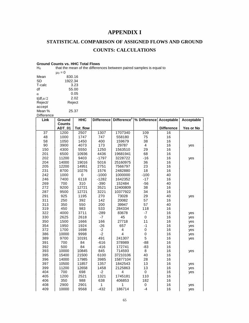
65

APPENDIX I

STATISTICAL COMPARISON OF ASSIGNED FLOWS AND GROUND

COUNTS: CALCULATIONS

Ground Counts vs. HHC Total FlowsH0 that the mean of the differences between paired samples is equal to

µD = 0Mean 830.16SD 1922.34T-calc 3.23df 55.00α 0.05t(df,α/2) 2.02Reject/accept

Reject

Mean %Difference

25.37

Link GroundCounts

HHC Difference Difference2 % Difference Acceptable Acceptable

ADT_01 Tot_flow Difference Yes or No37 1200 2507 1307 1707340 109 1648 1000 1747 747 558180 75 1658 1050 1450 400 159679 38 1690 3900 4073 173 29787 4 16 yes

150 4300 5550 1250 1563510 29 16201 6500 10936 4436 19681941 68 16202 11200 9403 -1797 3228722 -16 16 yes204 14000 19016 5016 25160975 36 16205 12200 14951 2751 7566797 23 16231 8700 10276 1576 2482880 18 16242 1000 0 -1000 1000000 -100 40246 7400 6118 -1282 1642352 -17 16269 700 310 -390 152484 -56 40272 9200 12721 3521 12400809 38 16287 9500 12721 3221 10377922 34 16291 925 1195 270 73028 29 40 yes311 250 392 142 20082 57 16313 350 550 200 39947 57 40319 450 983 533 284334 118 16322 4000 3711 -289 83678 -7 16 yes330 2625 2618 -7 45 0 16 yes350 1500 1666 166 27718 11 16 yes354 1950 1924 -26 657 -1 16 yes372 1700 1698 -2 4 0 16 yes386 10000 9998 -2 4 0 16 yes389 9700 10191 491 241307 5 16 yes391 700 84 -616 378989 -88 16392 500 84 -416 172741 -83 16393 10000 10845 845 714593 8 16 yes395 15400 21500 6100 37210106 40 16396 14000 17985 3985 15877104 28 16397 10500 11857 1357 1842543 13 16 yes399 11200 12658 1458 2125863 13 16 yes404 700 698 -2 4 0 16 yes405 1200 2521 1321 1745181 110 16406 350 988 638 406853 182 16408 2900 2901 1 1 0 16 yes409 10000 9568 -432 186714 -4 16 yes

66

410 9250 9353 103 10710 1 16 yes413 1500 1647 147 21609 10 16 yes416 3600 3711 111 12261 3 16 yes419 625 1182 557 309921 89 16420 950 325 -625 390074 -66 40421 5300 2487 -2813 7912996 -53 16428 5825 4633 -1192 1420052 -20 16432 8000 8026 26 679 0 16 yes433 6900 7280 380 144714 6 16 yes435 150 444 294 86572 196 16437 150 148 -2 4 -1 16 yes438 6800 6799 -1 1 0 16 yes439 2400 2400 0 0 0 16 yes441 3500 3255 -245 59985 -7 16 yes442 7913 11200 3287 10802463 42 16443 1400 4383 2983 8897343 213 16446 2700 2618 -82 6674 -3 16 yes454 3287 11200 7913 62620159 241 16SUM 273000 319489 46489 241841092 26 yes

gc:modelratio

0.85

Ground Counts vs. CLUSTER Total FlowsH0 that the mean of the differences between paired samples is equal to µD = 0Mean 910.03SD 1981.06T-calc 3.44df 55.00α 0.05t(df,α/2) 2.02Reject/accept

Reject

Mean %Difference

28.81

Link GroundCounts

CLUSTER Difference Difference2 % Difference Acceptable Acceptable

ADT_01 Tot_flow Difference Yes or No37 1200 2574 1374 1889056 115 1648 1000 1799 799 638496 80 1658 1050 1546 496 245882 47 1690 3900 4167 267 71463 7 16 yes

150 4300 5682 1382 1910306 32 16201 6500 11228 4728 22358379 73 16202 11200 9448 -1752 3070548 -16 16 yes204 14000 19404 5404 29208321 39 16205 12200 15193 2993 8955880 25 16231 8700 10271 1571 2469070 18 16242 1000 0 -1000 1000000 -100 40246 7400 6330 -1070 1145162 -14 16 yes269 700 336 -364 132822 -52 40272 9200 12901 3701 13700409 40 16287 9500 12901 3401 11569565 36 16291 925 1327 402 161213 43 40311 250 422 172 29701 69 16313 350 577 227 51413 65 40319 450 1102 652 425210 145 16322 4000 3800 -200 39850 -5 16 yes330 2625 2655 30 871 1 16 yes350 1500 1669 169 28728 11 16 yes354 1950 1991 41 1663 2 16 yes

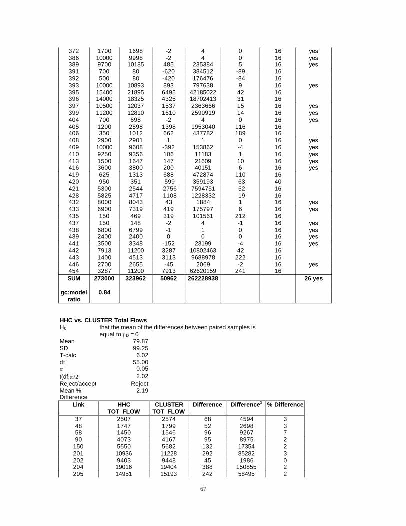
67

372 1700 1698 -2 4 0 16 yes386 10000 9998 -2 4 0 16 yes389 9700 10185 485 235384 5 16 yes391 700 80 -620 384512 -89 16392 500 80 -420 176476 -84 16393 10000 10893 893 797638 9 16 yes395 15400 21895 6495 42185022 42 16396 14000 18325 4325 18702413 31 16397 10500 12037 1537 2363666 15 16 yes399 11200 12810 1610 2590919 14 16 yes404 700 698 -2 4 0 16 yes405 1200 2598 1398 1953040 116 16406 350 1012 662 437782 189 16408 2900 2901 1 1 0 16 yes409 10000 9608 -392 153862 -4 16 yes410 9250 9356 106 11183 1 16 yes413 1500 1647 147 21609 10 16 yes416 3600 3800 200 40151 6 16 yes419 625 1313 688 472874 110 16420 950 351 -599 359193 -63 40421 5300 2544 -2756 7594751 -52 16428 5825 4717 -1108 1228332 -19 16432 8000 8043 43 1884 1 16 yes433 6900 7319 419 175797 6 16 yes435 150 469 319 101561 212 16437 150 148 -2 4 -1 16 yes438 6800 6799 -1 1 0 16 yes439 2400 2400 0 0 0 16 yes441 3500 3348 -152 23199 -4 16 yes442 7913 11200 3287 10802463 42 16443 1400 4513 3113 9688978 222 16446 2700 2655 -45 2069 -2 16 yes454 3287 11200 7913 62620159 241 16SUM 273000 323962 50962 262228938 26 yes

gc:modelratio

0.84

HHC vs. CLUSTER Total FlowsH0 that the mean of the differences between paired samples is

equal to µD = 0Mean 79.87SD 99.25T-calc 6.02df 55.00α 0.05t(df,α/2) 2.02Reject/accept RejectMean %Difference

2.19

Link HHC CLUSTER Difference Difference2 % DifferenceTOT_FLOW TOT_FLOW

37 2507 2574 68 4594 348 1747 1799 52 2698 358 1450 1546 96 9267 790 4073 4167 95 8975 2

150 5550 5682 132 17354 2201 10936 11228 292 85282 3202 9403 9448 45 1986 0204 19016 19404 388 150855 2205 14951 15193 242 58495 2

68

231 10276 10271 -4 19 0242 0 0 0 0 0246 6118 6330 211 44699 3269 310 336 26 678 8272 12721 12901 180 32374 1287 12721 12901 180 32374 1291 1195 1327 131 17233 11311 392 422 31 938 8313 550 577 27 722 5319 983 1102 119 14126 12322 3711 3800 90 8037 2330 2618 2655 36 1311 1350 1666 1669 3 9 0354 1924 1991 66 4412 3372 1698 1698 0 0 0386 9998 9998 0 0 0389 10191 10185 -6 37 0391 84 80 -4 20 -5392 84 80 -4 20 -5393 10845 10893 48 2282 0395 21500 21895 395 156018 2396 17985 18325 340 115614 2397 11857 12037 180 32407 2399 12658 12810 152 22982 1404 698 698 0 0 0405 2521 2598 76 5846 3406 988 1012 24 566 2408 2901 2901 0 0 0409 9568 9608 40 1588 0410 9353 9356 2 5 0413 1647 1647 0 0 0416 3711 3800 90 8037 2419 1182 1313 131 17149 11420 325 351 25 637 8421 2487 2544 57 3266 2428 4633 4717 83 6949 2432 8026 8043 17 301 0433 7280 7319 39 1511 1435 444 469 24 598 6437 148 148 0 0 0438 6799 6799 0 0 0439 2400 2400 0 0 0441 3255 3348 93 8576 3442 11200 11200 0 0 0443 4383 4513 130 16866 3446 2618 2655 36 1311 1454 11200 11200 0 0 0SUM 319489 323962 4473 899024

gc:modelratio

0.99