Using excel for business analysis

Using Excel forBusiness Analysis

ffirs 22 June 2012; 19:37:28

Founded in 1807, John Wiley & Sons is the oldest independent publishing company inthe United States. With offices in North America, Europe, Australia, and Asia, Wiley isglobally committed to developing and marketing print and electronic products andservices for our customers’ professional and personal knowledge and understanding.

The Wiley Finance series contains books written specifically for finance andinvestment professionals, as well as sophisticated individual investors and theirfinancial advisors. Book topics range from portfolio management to e-commerce,risk management, financial engineering, valuation, and financial instrument analysis,as well as much more.

For a list of available titles, please visit our website at www.WileyFinance.com.

http://www.WileyFinance.com

Using Excel forBusiness Analysis

A Guide to Financial Modelling Fundamentals

DANIELLE STEIN FAIRHURST

John Wiley & Sons Singapore Pte. Ltd.

Copyright ª 2012 John Wiley & Sons Singapore Pte. Ltd.

Published in 2012 by John Wiley & Sons Singapore Pte. Ltd. 1 Fusionopolis Walk,#07-01, Solaris South Tower, Singapore 138628

All rights reserved.

No part of this publication may be reproduced, stored in a retrieval system, or transmitted inany form or by any means, electronic, mechanical, photocopying, recording, scanning, orotherwise, except as expressly permitted by law, without either the prior written permissionof the Publisher, or authorization through payment of the appropriate photocopy fee to theCopyright Clearance Center. Requests for permission should be addressed to the Publisher,John Wiley & Sons (Asia) Pte. Ltd., 1 Fusionopolis Walk, #07-01, Solaris South Tower,Singapore 138628, tel: 65–6643–8000, fax: 65–6643–8008, e-mail: [email protected].

This publication is designed to provide accurate and authoritative information in regard tothe subject matter covered. It is sold with the understanding that the Publisher is not engagedin rendering professional services. If professional advice or other expert assistance is required,the services of a competent professional person should be sought. Neither the author nor thepublisher is liable for any actions prompted or caused by the information presented in this book.Any views expressed herein are those of the author and do not represent the views of theorganizations he works for.

Microsoft and Excel are registered trademarks of Microsoft Corporation.

Other Wiley Editorial OfficesJohn Wiley & Sons, 111 River Street, Hoboken, NJ 07030, USAJohn Wiley & Sons, The Atrium, Southern Gate, Chichester, West Sussex, P019 8SQ,

United KingdomJohn Wiley & Sons (Canada) Ltd., 5353 Dundas Street West, Suite 400, Toronto, Ontario, M9B

6HB, CanadaJohn Wiley & Sons Australia Ltd., 42 McDougall Street, Milton, Queensland 4064, AustraliaWiley-VCH, Boschstrasse 12, D-69469 Weinheim, Germany

978-1-118-13284-5 (Paper)978-1-118-13285-2 (ePDF)978-1-118-13286-9 (Mobi)978-1-118-13287-6 (ePub)

Typeset in 10/12pt, Sabon-Roman by MPS Limited, Chennai, India.Printed in Singapore by Ho Printing Singapore Pte. Ltd.

10 9 8 7 6 5 4 3 2 1

mailto:[email protected]

For Mike, of course.

Contents

Preface xi

CHAPTER 1What Is Financial Modelling? 1

What’s the Difference between a Spreadsheet and aFinancial Model? 3

Types and Purposes of Financial Models 4Tool Selection 5What Skills Do You Need to Be a Good Financial Modeller? 10The Ideal Financial Modeller 16Summary 19

CHAPTER 2Building a Model 21

Model Design 21The Golden Rules for Model Design 22Design Issues 24The Workbook Anatomy of a Model 25Project Planning Your Model 27Model Layout Flow Charting 28Steps to Building a Model 28Information Requests 35Version-Control Documentation 36Summary 37

CHAPTER 3Best Practice Principles of Modelling 39

Document Your Assumptions 39Linking, Not Hard Coding 39Only Enter Data Once 40Avoid Bad Habits 41Use Consistent Formulas 41Format and Label Clearly 41Methods and Tools of Assumptions Documentation 42Linked Dynamic Text Assumptions Documentation 48What Makes a Good Model? 51Summary 52

vii

CHAPTER 4Financial Modelling Techniques 53

The Problem with Excel 53Error Avoidance Strategies 54How Long Should a Formula Be? 59Linking to External Files 61Building Error Checks 63Avoid Error Displays in Formulas 66Circular References 67Summary 70

CHAPTER 5Using Excel in Financial Modelling 71

Formulas and Functions in Excel 71Excel Versions 73Handy Excel Shortcuts 74Basic Excel Functions 76Logical Functions 82Nesting: Combining Simple Functions to Create Complex Formulas 84Cell Referencing Best Practices 86Named Ranges 89Summary 92

CHAPTER 6Functions for Financial Modelling 93

Aggregation Functions 93LOOKUP Formulas 100Other Useful Functions 106Working with Dates 115Financial Project Evaluation Functions 121Loan Calculations 126Summary 131

CHAPTER 7Tools for Model Display 133

Basic Formatting 133Custom Formatting 133Conditional Formatting 139Sparklines 143Bulletproofing Your Model 147Customising the Display Settings 151Form Controls 157Summary 171

CHAPTER 8Tools for Financial Modelling 173

Hiding Sections of a Model 173Grouping 178

viii CONTENTS

Array Formulas 179Goal Seeking 184Pivot Tables 186Macros 190User-Defined Functions (UDFs) 198Summary 200

CHAPTER 9Common Uses of Tools in Financial Modelling 201

Escalation Methods for Modelling 201Understanding Nominal and Effective (Real) Rates 206Calculating Cumulative Totals 209How to Calculate a Payback Period 210Weighted Average Cost of Capital (WACC) 214Building a Tiering Table 216Modelling Depreciation Methods 219Break-Even Analysis 227Summary 233

CHAPTER 10Model Review 235

Rebuilding an Inherited Model 235Auditing a Financial Model 245Appendix 10.1: QA Log 250Summary 250

CHAPTER 11Stress-Testing, Scenarios, and Sensitivity Analysis in Financial Modelling 251

What’s the Difference between Scenario, Sensitivity,and What-If Analysis? 252

Overview of Scenario Analysis Tools and Methods 253Advanced Conditional Formatting 261Comparing Scenario Methods 264Summary 273

CHAPTER 12Presenting Model Output 275

Preparing an Oral Presentation for Model Results 275Preparing a Graphic or Written Presentation for Model Results 276Chart Types 279Working with Charts 291Handy Charting Hints 295Dynamic Range Names 297Charting with Two Different Axes and Chart Types 300

Contents ix

Bubble Charts 302Waterfall Charts 307Summary 316

About the Author 317

About the Website 319

Index 321

x CONTENTS

Preface

This book was written frommy course materials compiled over many years of trainingin analytical courses in Australia and globally—most frequently courses such as

Financial Modelling in Excel, Data Analysis & Reporting in Excel, and Budgeting &Forecasting in Excel, both as face-to-face workshops and online courses. The commontheme is the use of Microsoft Excel, and I’ve refined the content to suit the hundreds ofparticipants and their questions over the years. This content has been honed and refinedby the many participants on these courses, who are my intended readers. This book isaimed at you, the many people who seek financial analysis training (either by attendinga seminar or self-paced by reading this book) because you are seeking to improve yourskills to perform better in your current role, or get a new and better job.

When I started financial modelling in the early nineties, it was not called financialmodelling—it was just “Using Excel for Business Analysis,” and this is what I’ve calledthis book. It was only just after the new millennium that the term financial modellinggained popularity in its own right and became a required skill often listed on analyticaljob descriptions. This book spends quite a bit of time in Chapter 1 defining themeaning of a financial model as it’s often thought to be something that is far morecomplicated than it actually is. Many analysts I’ve met are building financial modelsalready without realising it, but they do themselves a disservice by not calling theirmodels, “models”!

However, those who are already building financial models are not necessarilyfollowing good modelling practice as they do so. Chapter 3 is dedicated to the prin-ciples of best modelling practice, which will save you a lot of time, effort, and anguishin the long run. Many of the principles of best practice are for the purpose of reducingthe possibility of error in your model, and there is a whole section on strategies forreducing error in Chapter 4.

The majority of Excel users are self-taught, and therefore many users will oftenknow highly advanced Excel tools, yet fail to understand how to use them in thecontext of building a financial model. This book is very detailed, so feel free to skipsections you already know. Because of the comprehensive nature of the book, much ofthe detailed but less commonly used content, such as instructions for the olderExcel 2003 users, has been moved to the companion website at www.wiley.com/go/steinfairhurst. References to the content on the website, and many cross-references toother sections of the book, can be found throughout the manuscript.

BOOK OVERVIEW

This book has 12 chapters, but these can be grouped into three parts. Whilst they dofollow on from each other with the most basic concepts at the beginning, feel free tojump directly to any of the parts. The first section—Chapters 1 to 3—addresses the

fpref 22 June 2012; 19:17:22

xi

http://www.wiley.com/go/steinfairhurst


least technical topics about financial modelling in general, such as tool selection, modeldesign, and best practice.

The second section—Chapters 4 to 8—is extremely practical and hands-on. Here Ihave outlined all of the tools, techniques, and functions in Excel that are commonlyused in financial modelling. Of course it does not cover everything Excel can do, but itcovers the “must-know” tools.

The third section—Chapters 9 to 12—is the most important in my view. Thiscovers the use of Excel in financial modelling and analysis. This is really where thebook differs from other “how-two” Excel books. Chapter 9 covers some commonlyused techniques in modelling, such as escalation, tiering tables, and depreciation—howto actually use Excel tools for something useful! Chapter 11 covers the several differentmethods of performing scenarios and sensitivity analysis (basically the whole point offinancial modelling to my mind!). Lastly, Chapter 12 covers the often-neglected task ofpresenting model output. Many modellers spend days or weeks on the calculations andfunctionality, but fail to spend just a few minutes or hours on charts, formatting, andlayout at the end of the process, even though this is what the user will see, interact with,and eventually use to judge the usefulness of the model.

ACKNOWLEDGEMENTS

This book would not have been written had it not been for the many people who haveattended my training sessions, participated in online courses, and contributed to theforums. Your continual feedback and enthusiasm for the subject inspired me to writethis book and it was through you that I realised how much a book like this was needed.

The continued support of my family made this project possible. In particular, Mikemy husband for his unconditional commitment and to whom this book is dedicated, mychildren who give me such joy, as well as my remarkable parents and siblings who havealways inspired and encouraged me without question. I would like to give a specialthanks to my ever-patient assistant Susan Wilkin for her dedication and diligencethroughout the project, Kurt Alexander for his steadfast enthusiasm, and to Joe Porteusfor keeping me on the right track.

I hope you find the book both useful and enjoyable. Happy modelling!

fpref 22 June 2012; 19:17:23

xii PREFACE

CHAPTER 1What Is Financial Modelling?

There are all sorts of complicated definitions of financial modelling, and in myexperience there is quite a bit of confusion around what a financial model is exactly.

A few years ago, we put together a Plum Solutions survey about the attitudes, trends,and uses of financial modelling, asked respondents “What do you think a financialmodel is?” Participants were asked to put down the first thing that came to mind,without any research or too much thinking about it. I found the responses interesting,amusing, and sometimes rather disturbing.

Some answers were overly complicated and highly technical:

n “Representation of behaviour/real-world observations through mathematicalapproach designed to anticipate range of outcomes.”

n “A set of structured calculations, written in a spreadsheet, used to analyse theoperational and financial characteristics of a business and/or its activities.”

n “Tool(s) used to set and manage a suite of variable assumptions in order to predictthe financial outcomes of an opportunity.”

n “A construct that encodes business rules, assumptions, and calculations enablinginformation, analysis, and insight to be drawn out and supported by quantitativefacts.”

n “A system of spreadsheets and formulas to achieve the level of record keeping andreporting required to be informed, up-to-date, and able to track finances accuratelyand plan for the future.”

Some philosophical:

n “A numerical story.”

Some incorrect:

n “Forecasting wealth by putting money away now/investing.”n “It is all about putting data into a nice format.”n “It is just a mega huge spreadsheet with fancy formulas that are streamlined to

make your life easier.”

Some ridiculous:

n “Something to do with money and fashion?”

c01 22 June 2012; 17:59:37

1

Some honest:

n “I really have no idea.”

And some downright profound:

n “A complex spreadsheet.”

Whilst there are many other (often very complicated and long-winded) definitionsavailable from different sources, but I actually prefer the last, very broad, but accuratedescription: “a complex spreadsheet.” Whilst it does need some definition, a financialmodel can pretty much be whatever you need it to be.

As long as a spreadsheet has inputs and outputs, and is dynamic and flexible—I’mhappy to call it a financial model! Pretty much the whole point of financial modelling isthat you change the inputs and the outputs. This is the major premise behind scenarioand sensitivity analysis—this is what Excel, with its algebraic logic, was made for!Most of the time, a model will contain financial information and serve the purposeof making a financial decision, but not always. Quite often it will contain a full set offinancial statements: profit and loss, cash flow, and balance sheet; but not always.

According to the more staid or traditional definitions of financial modelling, thefollowing items would all most certainly be classified as financial models:

n A business case that determines whether or not to go ahead with a project.n A five-year forecast showing profit and loss, cash flow, and balance sheet.n Pricing calculations to determine how much to bid for a new tender.n Investment analysis for a joint venture.

Butwhataboutotherpiecesof analysis thatweperformaspart of our roles?Can thesealso be called financialmodels?What if somethingdoes not contain financial informationat all? Consider if you were to produce a spreadsheet for the following purposes:

n An actual-versus-budget monthly variance analysis that does not contain scenariosand for which there are no real assumptions listed.

n A risk assessment, where you enter the risk, assign a likelihood to that risk, andcalculate the overall risk of the project using probability calculations. This does notcontain any financial outputs at all.

n A dashboard report showing a balance scorecard type of metrics reporting likeheadcount, quality, customer numbers, call volume, and so on. Again, there arefew or no financial outputs.

See the section on the “Types and Purposes of Financial Models” later in thischapter for some more detail on financial models that don’t actually contain financialinformation.

Don’t get hung up on whether you’re actually building something that meets thedefinition of a financial model or not. As long as you’ve got inputs and outputs thatchange flexibly and dynamically you can call it a financial model! If you’re using Excelto any extent whereby you are linking cells together, chances are you’re alreadybuilding a financial model—whether you realise it or not. The most important thing is

c01 22 June 2012; 17:59:38

2 USING EXCEL FOR BUSINESS ANALYSIS

that you are building the model (or whatever it’s called!) in a robust way, following theprinciples of best practice, which this book will teach you.

Generally, a model consists of one or more input variables along with data andformulas that are used to perform calculations, make predictions, or perform anynumber of solutions to business (or non-business) requirements. By changing the valuesof the input variables, you can do sensitivity testing and build scenarios to see whathappens when the inputs change.

Sometimes managers treat models as though they are able to produce the answer toall business decisions and solve all business problems. Whilst a good model can aidsignificantly, it’s important to remember that models are only as good as the data theycontain, and the answers they produce should not necessarily be taken at face value.

“The reliability of a spreadsheet is essentially the accuracy of the data that itproduces, and is compromised by the errors found in approximately 94% of spread-sheets.”1 When presented with a model, the savvy manager will query all theassumptions, and the way it’s built. Someone who has had some experience in buildingmodels will realise that they must be treated with caution. Models should be used asone tool in the decision-making process, rather than the definitive solution.

WHAT’S THE DIFFERENCE BETWEEN A SPREADSHEETAND A FINANCIAL MODEL?

Let me make one thing very clear: I am not partial to the use of the word spreadsheet; infact you’ll hardly find it used at all in this book.

I’ve often been asked the difference between the two, and there is a fine line ofdefinition between them. In a nutshell, an Excel spreadsheet is simply the medium thatwe can use to create a financial model.

At the most basic level, a financial model that has been built in Excel is simply acomplex spreadsheet. By definition, a financial model is a structure that contains inputdata and supplies outputs. By changing the input data, we can test the results of thesechanges on the output results, and this sort of sensitivity analysis is most easily done inan Excel spreadsheet.

One could argue then, that they are in fact the same thing; there is really no dif-ference between a spreadsheet and a financial model. Others question if it reallymatters what we call them as long as they do the job? After all, both involve puttingdata into Excel, organising it, formatting, adding some formulas, and creating someusable output. There are, however, some subtle differences to note.

1. “Spreadsheet” is a catchall term for any type of information stored in Excel,including a financial model. Therefore, a spreadsheet could really be anything—a checklist, a raw data output from an accounting system, a beautifully laid outmanagement report, or a financial model used to evaluate a new investment.

2. A financial model is more structured. A model contains a set of variableassumptions, inputs, outputs, calculations, scenarios, and often includes a set of

1Ruth McKeever, Kevin McDaid, Brian Bishop, “An Exploratory Analysis of the Impact ofNamed Ranges on the Debugging Performance of Novice Users,” European Spreadsheet RisksInterest Group: 2009. Available at arxiv.org/abs/0908.0935.

c01 22 June 2012; 17:59:38

What Is Financial Modelling? 3

standard financial forecasts such as a profit and loss, balance sheet, and cash flow,which are based on those assumptions.

3. A financial model is dynamic. A model contains variable inputs, which, whenchanged, impact the output results. A spreadsheet might be simply a report thataggregates information from other sources and assembles it into a useful presen-tation. It may contain a few formulas, such as a total at the bottom of a list ofexpenses or average cash spent over 12 months, but the results will depend ondirect inputs into those columns and rows. A financial model will always havebuilt-in flexibility to explore different outcomes in all financial reports based onchanging a few key inputs.

4. A spreadsheet is usually static. Once a spreadsheet is complete, it often becomes astand-alone report, and no further changes are made. A financial model, on theother hand, will always allow a user to change input variables and see the impactof these assumptions on the output.

5. A financial model will use relationships between several variables to create thefinancial report, and changing any or all of them will affect the output. Forexample, Revenue in Month 4 could be a result of Sales Price 3 Quantity SoldPrior Month 3 Monthly Growth in Quantities Sold. In this example, three factorscome into play, and the end user can explore different mixes of all three to see theresults and decide which reflects their business model best.

6. A spreadsheet shows actual historical data, whereas a financial model containshypothetical outcomes. A by-product of a well-built financial model is that we caneasily use it to perform scenario and sensitivity analysis. This is an importantoutcome of a financial model. What would happen if interest rates increase by halfa basis point? How much can we discount before we start making a loss?

In conclusion, a financial model is a complex type of spreadsheet, whilst aspreadsheet is a tool that can fulfill a variety of purposes—financial models being one.The list of attributes above can identify the spreadsheet as a financial model, but insome cases, we really are talking about the same thing. Take a look at the Excel filesyou are using. Are they dynamic, structured, and flexible, or have you simply created astatic, direct-input spreadsheet?

TYPES AND PURPOSES OF FINANCIAL MODELS

Models in Excel can be built for virtually any purpose—financial and non-financial,business- or non-business related—although the majority of models will be financialand business-related. The following are some examples of models that do not capturefinancial information:

n Risk Management: A model that captures, tracks, and reports on project risks,status, likelihood, impact, and mitigation. Conditional formatting is often inte-grated to make a colourful, interactive report.

n Project Planning: Models may be built to monitor progress on projects, includingcritical path schedules and even Gantt charts. (See the next section in this chapter,“Tool Selection,” for an analysis of whether Microsoft Project or Excel should beused for building this type of project plan.)

c01 22 June 2012; 17:59:38


n KPIs and Benchmarking: Excel is the best tool for pulling together KPI and metricsreporting. These sorts of statistics are often pulled from many different systems andsources, and Excel is often the common denominator between different systems.

n Dashboards: Popularity in dashboards has increased in recent years. The dash-board is a conglomeration of different measures (sometimes financial but oftennot), which are also often conveniently collated and displayed as charts and tablesusing Excel.

n Balanced Scorecards: These help provide a more comprehensive view of a businessby focusing on the operational, marketing, and developmental performance of theorganisation as well as financial measures. A scorecard will display measures suchas process performance, market share or penetration, and learning and skillsdevelopment, all of which are easily collated and displayed in Excel.

As with many Excel models, most of these could be more accurately created andmaintained in a purpose-built piece of software, but quite often the data for these kindsof reports is stored in different systems, and the most practical tool for pulling the datatogether and displaying it in a dynamic monthly report is Excel.

Although purists would not classify these as financial models, the way that theyhave been built should still follow the fundamentals of financial modelling bestpractices, such as linking and assumptions documentation. How we classify thesemodels is therefore simply a matter of semantics, and quite frankly I don’t think whatwe call them is particularly important! Going back to our original definition offinancial modelling, it is a structure (usually in Excel) that contains inputs and outputs,and is flexible and dynamic.

TOOL SELECTION

In this book we will use Excel exclusively, as that is most appropriate for the kind offinancial analysis we are performing when creating financial models. I recommendusing plain Excel, without relying on any other third-party software for several reasons:

n No extra licenses, training, or software download is required.n The software can be installed on almost any computer.n Little training is required, as most users have some familiarity with the product—

which means other people will be able to drive and understand your model.n It is a very flexible tool. If you can imagine it, you can probably do it in Excel

(within reason, of course).n Excel can report, model, and contrast virtually any data, from any source, all in

one report.n But most importantly, Excel is commonly used across all industries, countries, and

organisations. What this means to you is that if you have good financial modellingskills in Excel, these skills are going to make you more in demand—especially ifyou are considering changing industries or roles or getting a job in another country.

Excel has its limitations, of course, and Excel’s main downfall is the ease withwhich users can make errors in their models. Therefore, a large part of financialmodelling best practice relates to reducing the possibility for errors. See Chapter 3,

c01 22 June 2012; 17:59:38


“Best Practice Principles of Modelling,” and “Error Avoidance Strategies” in Chapter 4for details on errors and how to avoid them.

Is Excel Really the Best Option?

Before jumping straight in and creating your solution in Excel, it is worth consideringthat some solutions may be better built in other software, so take a moment tocontemplate your choice of software before designing a solution. There are many otherforms of modelling software on the market, and it might be worth consideringother options besides Excel. There are also a number of Excel add-ins provided by thirdparties that can be used to create financial models and perform financial analysis. Thebest choice depends on the solution you require.

The overall objective of a financial model determines the output as well as thecalculations or processing of input required by the model. Financial models are built forthe purpose of providing timely, accurate, and meaningful information to assist in thefinancial decision making process. As a result, the overall objective of the modeldepends on the specific decisions that are to be made based on the model’s output.

As different modelling tools lend themselves to different solutions or output, beforeselecting a modelling tool it is important to determine precisely what solution isrequired based on the identified model objective.

Evaluating Modelling Tools

Once the overall objective of the model has been established, a financial modelling toolthat will best suit the business requirements can be chosen.

To determine which financial modelling tool would best meet the identifiedobjective, the following must be considered:

n The output required from the model, based on who will use it and the particulardecisions to be made.

n The volume, complexity, type, and source of input data—particularly relating tothe number of interdependent variables and the relationships between them.

n The complexity of calculations or processing of input to be performed by the model.n The level of computer literacy of the users, as they should ideally be able to

manipulate the model without the assistance of a specialist.n The cost versus benefit set off for each modelling tool.

As with all software, financial modelling programs can either be purchased as apackage or developed in-house. Whilst purchasing software as a package is a cheaperoption, in a very complex industry, in-house development of specific modelling softwaremay be necessary in order to provide adequate solutions. In this instance, onewould needto engage a reputable specialist to plan and develop appropriate modelling software.

Which package you choose depends on the solution you require. A database orcustomer relationship management (CRM) data lends itself very well to a databasesuch as Microsoft Access, whereas something that requires complex calculations, suchas those in many financial models, is more appropriately dealt with in Excel.

Excel is often described as a Band-Aid solution, because it is such a flexible toolthat we can use to perform almost any process—albeit not as fast or as well as fully

c01 22 June 2012; 17:59:38


customised software, but it will get the job done until a long-term solution is found:“... spreadsheets will always fill the void between what a business needs today and theformal installed systems ... .”2

Budgeting and Forecasting

Many budgets and forecasts are built using Excel, but most major general ledger sys-tems have additional modules available that are built specifically for budgeting andforecasting. These tools provide a much easier, quicker method of creating budgetsand forecasts that is less error-prone than using templates. However, there aresurprisingly few companies that have a properly integrated, fully functioning budgetingand forecasting system, and the fallback solution is almost always Excel.

There are several reasons why many companies use Excel templates over a fullbudgeting and forecasting solution, whether they are integrated with their generalledger system or not.

n A full solution can be expensive and time-consuming to implement properly.n Integration with the general ledger system means a large investment in a particular

modelling system, which is difficult to change later.n Even if a system is not in place, invariably some analysis will need to be undertaken

in Excel, necessitating at least part of the process to be built using Excel templates.

Microsoft Office Tools: Excel, Access, and Project

Plain-vanilla Excel (and by this I mean no add-ins) is the most commonly used tool. Seethe next section for a review of some extra add-ins you might like to consider. How-ever, there are other Microsoft tools that could also serve to create the solution.Microsoft (MS) Access is probably the closest alternative to Excel, and quite oftensolutions are built in Excel when, in fact, Access is the most sensible solution.

There is often some resistance to using Access, and it is becoming less popular thanit was a decade or so ago. Prior to the release of Excel 2007, Excel users were restrictedto only 65,000 rows, and many analysts and finance staff used Access as a way to getaround this limit. With now over 1.1 million rows, Excel is able to handle a lot moredata, so there is less need for the additional row capacity of Access. However, Access isstill worth some consideration.

Advantages of Excel

n Excel is included most basic Microsoft packages (unlike Access, which often needsto be purchased separately) and therefore comes as standard on most PCs. Excel ismuch more flexible than Access and calculations are much easier to perform.

n It is generally faster to build a solution in Excel than in Access.n Excel has a wider knowledge base among users, and many people find it to be more

intuitive. This means it is quicker and easier to train staff in Excel.n It is very easy to create flexible reports and charts in Excel.

2Mel Glass, David Ford, Sebastian Dewhurst, “Reducing the Risk of Spreadsheet Usage �A Case Study,” European Spreadsheet Risks Interest Group: 2009. Available at arxiv.org/abs/0908.1584.

c01 22 June 2012; 17:59:38


arxiv.org/abs/0908.1584

n Excel can report, model, and contrast virtually any data, from any source, all inone file.

n Excel easily performs calculations on more than one row of data at a time, whichAccess has difficulty with.

Advantages of Access

n Access can handle much larger amounts of data: Excel 2003 is limited to 65,000rows and 256 columns, and Excel 2007 and 2010 are limited to around 1.1 millionrows and 16,000 columns. Access’s capability is much larger, and it also has agreater memory storage capacity.

n Data is stored only once in Access, making it work more efficiently.n Data can be entered into Access by more than one user at a time.n Access is a good at crunching and manipulating large volumes of data.n Due to Access’s lack of flexibility, it is a harder for users to make errors.n Access has user forms, which provide guidance to users and are an easy way for

users to enter data.

MS Project is specifically for creating project plans and associated componenttasks, assigning resources to those tasks, tracking progress, managing budgets, andmonitoring workloads. The user can also create critical path schedules andGantt charts.

Because the program handles costs, budgets, and baselines quite well, Project couldbe considered a viable alternative to a financial model, if the purpose of the model weresimply to create an actual-versus-budget tracking report. In fact, as with most purpose-built software, if your aim is to track andmonitor a project, Project is a far superior optionto Excel. Of course creating a project plan and even a Gantt chart is certainly possible inExcel, although it will take longer, and be far more prone to error than Project. There aremany reasons, however, why users will opt to use Excel for a project plan over Project:

n Project is not included in any of the Office suites and therefore needs to be pur-chased separately.

n The plan may need to be accessed, updated, and monitored by different users, whomay not be able to use Project due to lack of skills.

n For a reasonably small project it’s probably not worth the trouble; it’s simpler tojust work it up in Excel.

In summary, the choice between Excel and Project really depends on the size,scope, and complexity of the project plan model you are building. Bear in mind ofcourse that there are many other pieces of project planning software besides Project onthe market!

Excel Add-Ins Add-ins are programs that add optional commands and features to Excel.There are many add-ins on the market that have been developed specifically for thepurpose of financial modelling. For more complex calculations or processing of input,it may be useful to activate or install one or more add-ins, especially tools such asSolver, which are included in your MS Excel licence. Bear in mind that other users willprobably not have add-ins enabled, so they will not be able to see how your model hasbeen created or calculated.

c01 22 June 2012; 17:59:39


Excel add-ins can be categorised according to source:

n Add-ins such as Solver and the Analysis ToolPak that only need to be activatedonce Excel has been installed.

n Add-ins that must be downloaded from Office.com and installed before they canbe used.

n Custom add-ins created by third parties that must be installed before they can beused: Component Object Model (COM) add-ins, Visual Basic for Applications(VBA) add-ins, Automation add-ins, or DLL add-ins.

Excel add-ins from all sources can be used to perform a variety of tasks that assistin the financial modelling process. These add-ins can be broadly defined as:

n Standard Excel add-ins such as the Analysis ToolPak and Solver.n Audit tools.n Integration links between Excel and the general ledger system.

The most commonly used add-ins are the Analysis ToolPak and Solver, which arestandard add-in programs that are available when you install Microsoft Office orExcel. They are included in the program but are disabled by default, so if you want touse them, you need to enable them.

Prior to the release of Excel 2007 the only way to access certain functions (e.g.,¼EOMONTH and ¼SUMIFS) in Excel 2003 was to download the Analysis ToolPak.However, these functions are now standard in Excel 2007 and later, so the AnalysisToolPak is now less commonly used.

Other features in the Analysis ToolPak are tools like Data Analysis ToolPak, whichhas some powerful statistical and engineering functions not commonly used in financialmodelling. Solver, however, is an extremely useful but rather advanced tool for cal-culating optimal values in financial modelling.

Audit Add-Ins Audit add-ins for Excel are used to ensure the accuracy of data and cal-culations within a spreadsheet or workbook. They can very quickly identify formulaerrors by looking at inconsistent formulas, comparing versions, and getting to thebottom of complex named ranges. There are several custom add-ins available both fromMicrosoft and other parties that will facilitate accuracy by performing formula inves-tigations, precedent/dependent analysis, worksheet analysis, and sensitivity reporting.

Whilst they can assist with checking for formula errors, there are many other typesof errors that can be easily overlooked, and using these add-ins can provide a falsesense of security. See the section on “Error Avoidance Strategies” in Chapter 4 for moredetail.

Integration Add-Ins Integration add-ins allow information from the financial reportingsystem to be transferred into Excel for further analysis, or data stored in Excel to betransferred into the financial reporting system. These are often used for the purpose of:

n Transferring information from the general ledger system into Excel for the pur-poses of reporting and analysis. Many management reports are built in Excel, andextract up-to-date data directly from the general ledger system into the reports.

c01 22 June 2012; 17:59:39


http://Office.com

n Loading information in the form of journal entries back into the general ledgersystem. Data is often manipulated in Excel, and then loaded into the generalledger as a journal. For example, if an invoice needs to be split between differentdepartments based on headcount allocation, this calculation might be done inExcel, split to departments in the journal, and loaded into the general ledgersystem.

The Final Decision

The more sophisticated a financial model is, the more expensive it is to maintain. It istherefore best to use a model with the lowest possible level of sophistication needed toprovide a specific solution. For this reason, purchasing a software package, provided itcan provide the desired solution, would usually be advisable.

Once the decision has been made to purchase a software package, it must be deter-mined which package will provide the best solution as certain solutions may be betterprovided by particular software packages.

There are many forms of software and Excel add-ins on the market that can beused to create financial models. However, provided that it can provide an adequatesolution, we recommend using plain Excel, as it is easy to use and no extra licenses,training, or software downloads are required. If additional functionality is needed,Excel add-ins may be considered.

WHAT SKILLS DO YOU NEED TO BE A GOOD FINANCIAL MODELLER?

When you decide your financial models are not as good as they should be, should youimmediately take an advanced Excel course? Whilst this is helpful, there’s a great dealmore to financial modelling than being good at Excel!

When considering the skills that make up a good financial modeller, we need todifferentiate between conceptual modelling, which is to have an understanding of thetransaction, business, or product being modelled, and spreadsheet engineering, which isthe representation of that conceptual model in a spreadsheet. Spreadsheet skills arereasonably easy to find, but a modeller who can understand the concept of the purposeof the model and translate it into a clear, concise, and well-structured model ismuch rarer.

People who need to build a financial model sometimes think they need to becomeeither an Excel super-user or an accounting pro who knows every in and out ofaccounting rules. I’d argue you need a blend of both, as well as a number of other skills,including some business common sense!

Spreadsheet and Technical Excel Skills

It’s very easy for financial modellers to get bogged down in the technical Excel aspectsof their model, get carried away with complex formulas, and not focus on key high-level, best-practice procedures, such as error-checking strategies and model stress-testing.

Excel is an incredibly powerful tool, and almost no single Excel user will have theneed or desire to utilise most of the functionality this program offers. As with most

c01 22 June 2012; 17:59:39


software, the 80/20 rule applies: 80 percent of users use only 20 percent of thefeatures—although some would argue that 95 percent of Excel users use only 5 percentof the features! Still, there are those select fewwho understand every in and out of Excel,every single function, and work out how to do practically anything in Excel. Do youneed to have this level of Excel skill to become a good financial modeller? Unfortu-nately, having great software skills doesn’t always help when it comes to applying themto a specific area of business. Realise that Excel is used in several capacities, so being anExcel super-user doesn’t automatically mean you’ll be a super financial modeller. Thebest financial models are clear, well structured, flexible, and dynamic; they are notalways the biggest and most complicated models that use the most advanced tools andfunctions! Many of the best financial models use only Excel’s core functionality.

Having said that, to be a good financial modeller, you do need to know Excelexceptionally well. Those people who maintain that you don’t need good Excel skills tobe a financial modeller are usually those with weak Excel skills. You should be buildinga superb model using simple and straightforward tools because you’ve chosen to makeyour model clear and easy to follow, not because that’s all you know how to do! Youdon’t have to be a super-user—the 99th percentile in Excel knowledge—but you mustcertainly be above average. A complex financial model might use features in Excel thatthe everyday user doesn’t know. The best financial model will always use the solutionthat is the simplest tool to complete the task (as simple as possible and as complex asnecessary, right?), so the more familiar you are with the tools available in Excel, theeasier it will be. An array formula or a macro might be the only way to achieve whatyou need to achieve, but a simpler solution may well be—and often is—superior. Youmight also need to take apart someone else’s model, which uses complex tools, and it’svery difficult to manipulate an array formula or a macro if you’ve never seen onebefore! So, if you are considering a career as a financial modeller (as I assume you are)improving your Excel knowledge is an excellent place to start.

EXAMPLES OF TECHNICAL EXCEL SKILLS QUESTIONS

n Howdo I use the appropriate formula? For example, should I use aVLOOKUPor a SUMIF?

n Howdo I insert or hide a sheet and thenprotect it so that the user can’t access it?

n How do I construct a complex but concise formula?

Industry Knowledge

One of the fantastic things about financial modelling is that it is applicable across somany different industries. Good financial modelling skills will always stand you ingood stead, no matter which industry or country you are working in! Financialmodelling consultants or generalists will probably work in many different industriesduring their careers and be able to build models for different products and services.They will probably not be experts in the intricacies of each industry, however, andthat’s why it’s important for a financial modelling generalist to consult carefully with

c01 22 June 2012; 17:59:39


the subject matter expert for the inputs, assumptions, and logic of the financial model.Don’t be afraid to ask lots and lots of questions if the details are not absolutely clear.It’s quite likely that the person who has commissioned the model hasn’t actuallythought through the steps, inputs, assumptions, and even what the outputs should looklike, until you ask the right question.

Financial modellers working within an organisation, however, usually becomeexperts in their own industry or domain, and will become very familiar with theminutiae of how financial models for that industry should be designed, and whichassumptions should be used.

Financial modelling consultants are very careful to transfer responsibility for theassumptions to the end user, which is a very sensible course of action. The personbuilding the model is often not the one who has commissioned it or the person who isactually using it. Model builders are often not overly familiar with the product or eventhe organisation, and they cannot (and should not) take responsibility for the inputs.(See the section “Document Your Assumptions” in Chapter 3 for greater detail on theimportance of documentation of assumptions.)

For example, when building a pricing model, the modeller needs to understand theproduct and how the costs and revenue work. Experience with regulatory constraintswill help the modeller to understand the basis of regulation and its components (e.g.,cost building blocks, cost index, revenue cap, weighted average price cap, maximumprices, etc.). Understanding of economic concepts, such as efficient cost calculation,return on and of a regulatory asset base, operating costs and working capital, long-runversus short-run marginal costs, and average costs, are other examples of industryknowledge that is useful for the financial modeller.

EXAMPLES OF INDUSTRY KNOWLEDGE

n Regulatory constraints.

n Industry standards.

n Maximum price that can be charged for a certain item.

Accounting Knowledge

Elements such as financial statements, cash flow, and tax calculations can be animportant aspect of many financial models. Professional accountants know every singleaccounting rule and law there are, so are they good financial modellers? If a highlyskilled accountant built a financial model, you would guess that the layout andstructure of the financial statements will be 100 percent correct, but will they be linkedproperly? If you change some of the inputs, does the balance sheet still balance?Sometimes not! A good accountant, or even someone qualified with a master of appliedfinance, might not be familiar with all of the modelling technical tools, even if they area competent Excel user. As with the other modelling skills, you don’t need a top level ofaccounting knowledge to build a financial model. In fact, financial models are often

c01 22 June 2012; 17:59:39


relatively straightforward from an accounting standpoint. You certainly do not need tobe a qualified accountant to become a financial modeller, although a good under-standing of accounting and knowledge of finance certainly help.

There are some situations where industry knowledge and accounting are required forfinancial modelling. For example, in manufacturing or, particularly, in the oil and gasindustry, the modeller needs to know whether FIFO (first in, first out) or LIFO (last in,first out) accounting is being used, as this has a big impact on the way that inventoryis being modelled. A financial modeller who has never worked in these industriesmay not have ever heard of FIFO and LIFO, and would probably have no idea how tomodel it.

EXAMPLES OF ACCOUNTING KNOWLEDGE

n How is a profit-and-loss statement structured?

n How do I construct a cash-flow forecast from my model?

n How do I turn capital expenditure into a depreciation expense?

Business Knowledge

Amodeller with wide-ranging business experience is well equipped to probe for the factsand assumptions that are critical for building a financial model. This is probably the mostdifficult skill to teach, as it’s most easily picked up by working in a management role.

Business acumen is particularly important when commissioning, designing, andinterpreting a financial model. When creating the model, the modeller needs to con-sider the purpose of the model. What does the model need to tell us? Knowing thedesired outcome will assist with the model’s build, design, and inputs. If, for example,we are building a pricing model, we need to consider the desired outcome; normally,the price we need to charge in order to achieve a certain profit margin. What is anacceptable margin? What costs should we include? What cost will the market bear?Modellers should also have an understanding of economic concepts, such as efficientcosts and how these are calculated, an expected return on an asset base, operating costsand working capital, or long-run versus short-run marginal costs.

Of course the answers to these questions can be obtained from other people, but amodeller with good business sense will have an innate sense of how a model should bebuilt, and what is the most logical design and layout to achieve the necessary results.

EXAMPLES OF BUSINESS KNOWLEDGE

n What is cost of capital and how does that affect a business case?

n Which numbers are important?

n What does the internal rate of return (IRR)mean andwhat is an acceptable rate?

c01 22 June 2012; 17:59:40


Aesthetic Design Skills

This is an area that many modellers and analysts struggle with, as aesthetics simply donot come naturally to left-brain thinkers like us. We are mostly so concerned withaccuracy and functionality that we fail to realise that the model looks—and I’m notgoing to mince words here—ugly! Although it’s just a simple matter of taking our timewhen formatting, most of us could not be bothered with such trivial details as makingmodels pretty, and consequently most models I see use the standard gridlines, font, andblack-and-white colouring that are Excel defaults. I’m certainly not suggesting that youembellish your models with garish colours, but you should take some pride in yourmodel. See the section on “Bulletproofing Your Model” in Chapter 7 for some ideas onhow to remove gridlines and change some of the standard settings so that your modellooks less like a clunky spreadsheet and more like a reliable, well-crafted model you’vetaken your time over. Research shows that users place greater faith on models withaesthetic formatting than those without, so one of the fastest and easiest ways to giveyour model credibility is to simply spend a few minutes on the colours, font, layout,and design.

Some aesthetic formatting is critical for the functionality and to avoid error (seesection on “Error Avoidance Strategies” in Chapter 4), but mostly it adds credibilityand makes your model easier to work with.

Models can become complex very quickly and without a well-planned design theycan be unintelligible. Some basic components of a model should be a cover sheet,instructions, and clearly labelled inputs, outputs, workings, and results. For extremelylong and complex models with many sheets, a hyperlinked table of contents is also avaluable addition to help the user navigate the model.

Communication and Language Skills

This is also an area that we left-brain thinkers are not always good at. Some analystslike to lock themselves away, working on spreadsheets without communicating withother people. If this is your tendency, then you might need to consider whetherfinancial modelling is a good career choice for you, because there is a surprisingamount of human interaction required for most financial modellers.

n Assumptions Validation: In order to gain buy-in from stakeholders, the keyassumptions and inputs often need to be communicated verbally or in writing.People in various parts of the business should be involved in order to check theaccuracy and appropriateness of inputs for inclusion in a model. Stakeholders willoften query the assumptions or the way they have been used and provide extremelyvaluable insight for modellers (particularly for a consultant or modeller with littleindustry or product knowledge). Performing this task well is a critical step in themodelling process.

n Data Gathering: There are some modelling projects where more time is spentgathering and collating data than actually building the model. Holders of infor-mation can be guarded about giving access to data, sometimes irrationally, butoften it’s because they’ve had bad experiences in the past. This can occur whensomeone provides estimates off the record, and later discovers that those numbershave been used in budgets or other documents to which they are held accountable.

c01 22 June 2012; 17:59:40


So, people can be understandably reticent about providing data when requested foran ad hoc project such as a financial model. A modeller with good communicationskills will be able to dig, delve, and coax the information out of them!

n Presentation Skills: Senior management, when approving a project, often wants tohear about the financial implications of the project from the person who actuallybuilt the model, and so modellers are sometimes required to present the key out-comes to a board or executive committee. Being able to distill a 30-megabyte,extremely complex financial model that contains 20 tabs and took you six weeks tobuild, into three PowerPoint slides and a six-minute summary presentation can bequite a challenge!

n Client Skills: Whether you are a consultant or an in-house employee, working wellwith clients is a useful skill. Even in-house modellers have clients; every person youwork with or for should be considered a client and treated with the same respectand consideration as though they were paying your bill.

In all of these interactions with other people, financial modellers must show con-fidence in their model. Build the model to the best of your ability. Use best practices,check for errors, and follow a good and logical thought process, so thatwhen you presentor discuss your model, you can do so in a way that exudes absolute confidence. Doing soreduces questions about the accuracy, usefulness, and validity of your model. Be honestabout the fallibility of your model and its known shortcomings (let’s face it, no model isperfect), but be confident that you have built it to best-practice standards within thelimitations of time, data, or scope. This will serve to increase your model’s credibility,building your reputation within your company, and, of course, enhancing your career!

Numeracy Skills

Financial models, of course, have a significant mathematical component, and peoplewith good numeracy skills are best suited to it. Solid math skills can be particularlyuseful in error-checking and sense-checking. The ability to make rough estimatesquickly means they will be able to spot errors more easily. If we sell 450 units at $800each, will our sales revenue be $3.6 m, or $360,000? If we’ve made a calculation error,the numerate modeller will pick up the mistake much more quickly.

The numerate modeller will also have a gut feel for differentiating between criticalassumptions that need further verification, and input that is insignificant or immaterialto the model. The less-numerate modeller will have to test it manually, and will probablyend up with the same result, but it will take longer!

General numeracy is a skill that is difficult to teach, and one that can be easilytested for in the recruitment process. Experience working with models over timecan drastically improve these skills as the modeller who is less numerate will learnways to compensate through error-testing, and these techniques will become acquired,innate habits.

Ability to Think Logically

Modelling is often like programming, and complex logic needs to be interpreted intothe language of Excel so that the program can understand and create the modeller’sexpected results. For example, if we want to show a value, but only if the cell being

c01 22 June 2012; 17:59:40


tested is in the future, we would vocalise it by saying: “Show me the value, but only ifthe test cell is greater than or equal to today’s date.” The way that we need to translatethis into Excel’s language is to use the formula:

¼IF(test_cell.¼today,value,0).

Logic is also critical for model layout, design, and the use of assumptions in cal-culations. The issue of timing in annual models is one that I use often when demon-strating logic in my training workshops. If we are estimating the revenue for a newinsurance product, and the assumption is that we acquire 30,000 customers every year,we can’t assume revenue for the full 30,000 customers, as not all of them will begin onthe very first day of Year 1. Customers will be acquired gradually throughout the year,so we need to take an average in order to calculate revenue. This is an example of howit is very easy to get logic wrong, and overestimate revenue by a substantial amount.

Logic is one of those analytical skills that is very difficult to teach, but modellers whohave made a logic error (like the one illustrated above) learn quickly from their mistakesand are quite careful to use clear, well-documented logic for others to follow and check.

THE IDEAL FINANCIAL MODELLER

In general, most modellers have at least some of the aforementioned skills, and at timesit is necessary to consult specialists in order to create a successful financial model.Having read the section on the skills that you need to be a good financial modeller, youshould have a fairly good idea about which areas you are lacking in. Once you haveidentified these areas, you can work to improve them and liaise with other specialists toensure that your model is not lacking as a result of your weaknesses.

What financial modellers bring to the table is a combination of skills. First, they knowExcel well enough to be able to choose the simplest and most functional tool to build amodel. They can create a pivot table, array formula, or macro (but only when necessary,of course!); use a simple or complex nested formula; and choose the best technical toolto perform a scenario analysis. They also understand all the relevant business andaccounting principles. At the end of the day, the balance sheet has to balance, and theending cash on your cash flow statement needs to tie to the balance sheet, for example.

The ideal financial modeller brings a unique combination of skills that neither anExcel guru nor an accounting whiz possesses. He or she understands sensitivity andrelationships between variables, how fluctuations in inputs will impact the outcomes, andhow this needs to bemodelled in Excel. A financial modeller can also take a step back andrealisewhat the ultimate goal of themodel shouldbe.Arewebuilding amodel for in-houseuse, or to present to investors? Do we need a valuation, a variance analysis, a nice sum-mary, or a detailed, month-by-month profit-and-loss report? The financial modeller cantake information, build an Excel model that is technically correct from an accountingstandpoint, set up themodel, and ultimately reflectwhat the business is looking to achieve.

What’s the Typical Background for a Financial Modeller?

A key problem in the financial modelling industry is that modelling is often incorrectlyconsidered a junior task, and is often given to inexperienced graduate analysts whoundoubtedly have good Excel skills, but simply do not have the depth of business

c01 22 June 2012; 17:59:40


experience to create good financial models. If a modeller is able to tick all of the aboveboxes (i.e., good financial skills, good communicator, able to resolve ambiguity), he orshe is likely to quickly move into a more senior position to execute more managementresponsibilities and spend less time building financial models.

Most financial modellers come from a finance background and have graduallybeen exposed to industry knowledge. They often become specialists in a field, pickingup business acumen, communication skills, and logic along the way. Quite oftenengineers, project managers, construction specialists, or even scientists who arerequired to build their own financial models end up pursuing a career in financialmodelling. They have the industry and product knowledge and are able to learn theExcel skills, but may struggle with the finance side of things. Some would argue that itis easier to teach an engineer or scientist financial skills than it is to teach a financialaccountant about the industry, but I think both have a tough job. Every modellerwill have strengths and weaknesses, but a good financial modeller will span differentskill sets and will have a little bit of everything.

Training Courses

As a specialist financial modelling consultant and trainer, I spend a lot of my timerunning training courses and, consequently, many people expect me to be a firmadvocate of the face-to-face training workshop, right? Not necessarily. I’ve come underfire from my training partners in the past for publicising this opinion, but I’m notentirely convinced that going on a training course is always the best option for someonekeen to improve their financial modelling skills.

Excel is the backbone to any custom-built financial model, and as discussed in theprevious section, one of the core attributes of a financial modeller is to have goodtechnical Excel skills. When struggling with financial models, some managers’ firstreaction is to send their staff on an advanced Excel course to improve their modellingskills. However, with training budgets under constant scrutiny, you really need to makesure that you get the best value out of your training options. Is a training course reallywhat you need?

When considering an advanced Excel course, there are a few points you shouldconsider.

n As financial modellers, our use of Excel is quite narrow. I know it’s hard for us toconceive, but there is a whole world of Excel outside the finance industry! Sta-tisticians, database programmers, and engineers, to name a few, are able to useExcel’s advanced functions to create non-financial spreadsheets. Most advancedExcel courses are very broad, and will cover functions and capabilities that do notapply to your needs as a financial modeller. You may learn a few tricks, but thetime and money spent could be invested elsewhere.

n Research shows that a large percentage of the skills learned in training courses are notretained. Will you really remember everything that you learn? A programme ofcontinuous, applied learning is oftenmore effective than an intensive training course.

n Are your Excel skills really the problem? Following best practices and masteringthe logic behind a financial model are more important than building in complexformulas and, for the most part, you will want to keep formulas as simple aspossible.

c01 22 June 2012; 17:59:40


Alternatives to Attending a Training Course Other options to improve your financialmodelling skills without going on an advanced Excel course include:

n Read a book! Buying this book is a great start. You’ll still have it to refer to whenthe excitement and enthusiasm you felt after completing a training course are longgone, and you’re back to struggling with building your financial models.

n Take an interest in what work your colleagues have done and how they did it—youcan always learn from the techniques of others.

n Read, use, anddissect other people’smodels. Sometimes the bestway to learn is to seewhat someone else has done. Try taking someone else’s model apart and see how heor she built it. It’s probably best to use your company’s models, but if you don’t haveaccess to those, take a look at some of the sample models provided on this book’scompanion website, which can be found at www.wiley.com/go/steinfairhurst.

n Read specialist financial modelling publications or subscribe to e-mail newslettersabout using Excel. They often contain useful articles about specific techniques andtips that can enhance your skills. Getting a short e-mail tip every day is much moreeffective than reading many all at once. You’ll retain the information better in bite-size pieces.

n Search online. If you’re struggling with a formula or layout problem and areconvinced that there must be an easier way to do something, there usually is!Chances are that others have had the same problem in the past and, if you’re lucky,they’ve documented it as a blog post. There are some fantastic, publicly availableonline resources including tutorials, articles, blogs, forums, and videos specialisingin Excel and financial modelling that can be used at your convenience rather thantaking an entire day or two to attend a course. You will find links to some of myfavorite websites and online resources listed on the companion website at www.wiley.com/go/steinfairhurst.

Select the Right Training Option for You The strategies outlined here are great for con-tinually improving your Excel and financial modelling skill set, and they certainlywon’t break the budget, but what if you really need to give your skills a quick boost toget you ready for an upcoming project? There are a number of options available:

n Try to find a course specifically aimed at Excel for financial modellers, and—evenbetter—find one dedicated to your industry. Although good financial modellingskills are relevant across many different industries, there is nothing like specialisedtraining dedicated to the modelling issues inherent in your own industry. In recentyears, many more specialist financial modelling courses have become available,especially in major cities.

n If your company is able to arrange a group in-house training course, this will beeven better, as you may be able to learn with the templates and models actuallyused within your organisation. You also have the added advantage of choosing atime and location that suit you.

n If you can afford a private session, this is the most convenient and time-efficientmethod, as you can ask questions and cover only topics that are useful toyou. Many specialist training companies provide Excel one-on-one mentoringsessions.

c01 22 June 2012; 17:59:40





Do You Really Need an Advanced Excel Course?

It’s true that “you don’t know what you don’t know,” and so some people go ontraining courses because they want to make sure there isn’t something about the subjectthat they are missing. Having heard or seen something in a training course gives youexposure to something that you might never have heard about, but if it’s simplyinspiration you’re after, a good newsletter might well suffice (and be a lot cheaper)!

You might learn a few tricks on a course, but most people have got to think reallyhard before spending the money and taking a day or two out of their schedules tocommit to training workshops. There is no question that face-to-face workshops arevery effective; for many people, they are the best way to learn. However, I wouldrecommend that potential attendees exhaust the available blogs, forums, and news-letters first.

In summary, an advanced Excel course would certainly benefit those who plan onextensively using Excel in their role for multiple purposes. However, if your mainobjective is to become an expert financial modeller, focus instead on mastering the fewtools you need—such as logic and methodology—either in a course or via anothermedium, rather than expending time and money to learn things you may not use.

SUMMARY

In this chapter, we have discussed the definition of a financial model, and determinedthat, at a basic level, a financial model is really just a complex spreadsheet that containsinputs and outputs in a dynamic way. However, not every spreadsheet could be called afinancial model. Models in Excel can be built for virtually any purpose, both financialand non-financial, business or non-business, although the majority of models will befinancial- and business-related—and these are the kinds of examples we will mainlyfocus on.

Although this book is about how to use Excel in the context of business analysisand financial modelling, consider that there are many other available modelling toolsbesides Excel, including Microsoft products, add-ins, and third-party software. Excel isthe most commonly used software for this type of analysis, and in terms of buildingyour skill set, improving your Excel skills will always stand you in good stead for acareer in finance.

Having good technical Excel skills is not the only attribute of a good financialmodeller; industry knowledge, accounting, business acumen, design skills, communi-cation, logic, and numeracy are also important. Modellers will have all of these skills invarying degrees, so think about which skills you need to work on the most. Going to atraining course; using and taking apart others’ models; reading specialist publicationsand blogs; and using other online resources are all great ways to improve your financialmodelling skills.

c01 22 June 2012; 17:59:40


c01 22 June 2012; 17:59:40

CHAPTER 2Building a Model

Before launching in to build a model, it’s important to think about model design,structure, layout, and planning. A thought-out design and clear project plan can

make a huge difference to the quality and success of the modelling project.

MODEL DESIGN

Design can sometimes be the most difficult part of building a financial model and, inmy experience, one of the most difficult to teach and learn. The best way to developdesign skills is to critically assess other people’s models, taking note of what works anddoesn’t, and then applying it to your own models.

Even the simplest models can become complex if poorly designed, and a well-designed model will be so straightforwardly logical that it will simply speak for itself.It’s pretty easy to just dive in and start building a model without thinking aboutthe implications of the design. It’s not a bad idea to spend some time thinking about thelayout before you get started. The layout and structure of the model relate to the lookand feel of the model, and how users navigate through the model.

The following examples outline a couple of different challenges you might comeacross when designing the layout of a model.

Practical Example 1—Assumptions Layout

Let’s say you are creating a high-level five-year forecast. We’ve got 15,065 customersin 2013, and we are expecting that number to increase by 5 percent every year. Ifyou set up your model as shown in Layout Option 1 in Figure 2.1, with only onegrowth assumption, you’re very much restricted to a single input for the growthnumber.

If we change the design of the calculations by adding multiple input assumptioncells, and change the formula just a little, we are making our model a lot more flexibleand useful in the long term. This way if we decide to change the growth number foreach year, as shown in Figure 2.2 below, we won’t need to change any of our formulasin the future, and our model is much more robust and less prone to error.

Of course Layout Option 2 is slightly more complex, but is more functional for theuser. This example demonstrates the constant balance that a modeller needs tomaintain between functionality and simplicity when building a financial model.

c02 22 June 2012; 18:1:48

21

Practical Example 2—Summary Categorisation

Arranging products to display into categories in a model is another potentially difficultmodel layout problem. Let’s say you’re creating a pricing model for some advertisingproducts. You’ve got print ads and digital ads, and these are both split into Display andText Only. The question is, should you display the output of the model as shown inFigure 2.3 or Figure 2.4?

The example in Figure 2.4 is more concise, but shows less detail, so it reallydepends on how much detail you want to show your user. This comparison demon-strates the constant balance that a modeller needs to maintain between detail andconciseness when building a financial model.

THE GOLDEN RULES FOR MODEL DESIGN

There are a few rules for model design that should be followed when designing thelayout of a model. Most experienced modellers will follow these instinctively, as theyare generally common sense.

FIGURE 2.2 Model Layout Option 2

FIGURE 2.1 Model Layout Option 1

c02 22 June 2012; 18:1:48


Separate Inputs, Calculations, and Results, Where Possible

Clearly label which sections of the model contain inputs, calculations, and results. Theycan be on separate worksheets or separate places on a given worksheet, but make surethat the user knows exactly what each section is for. Colour coding can help withensuring that each section is clearly defined.

See the forthcoming section titled “The Workbook Anatomy of a Model” for morediscussion on whether it is always practical to separate these sections.

Use Each Column for the Same Purpose

This is particularly important when doing models involving time series. For example, ina time-series model, knowing that labels are in Column B, unit data in Column C,constant values in Column D, and calculations in Column E, makes it much easierwhen editing a formula manually.

Use One Formula per Row or Column

This forms the basis of the best-practice principle whereby formulas are kept consistentusing absolute, relative, and mixed referencing, as described in more detail inChapter 3, “Best Practice Principles of Modelling.” Keep formulas consistent whenin a block of data, and never change a formula halfway through.

FIGURE 2.3 Model Categorisation Option 1

FIGURE 2.4 Model Categorisation Option 2

c02 22 June 2012; 18:1:48

Building a Model 23

Refer to the Left and Above

The model should read logically, like a book, meaning that it should be read from left toright and top to bottom. Calculations, inputs, and outputs should flow logically to avoidcircular referencing. Be aware that there are times when left-to-right or top-to-bottomdata flow can conflict somewhat with ease of use and presentation, so use commonsense when designing the layout. By following this practice, we can avoid having cal-culations link all over the sheet, which makes it harder to check and update.

Use Multiple Worksheets

Avoid the temptation to put everything onto one sheet. Especially where blocks ofcalculations are the same, use separate sheets for those that must be repeated to avoidthe need to scroll across the screen.

Include Documentation Sheets

A documentation sheet where assumptions and source data are clearly laid out is acritical part of any financial model. A cover sheet should not be confused with anassumptions sheet. Document, document, document!

DESIGN ISSUES

Here are four key issues you need to think about before you start a model.

1. Time Series: Most financial models include a time-series element, and the majorityof these will be either monthly, quarterly, or annual. It’s important to get this rightfrom the start, as it’s much easier to summarise a monthly model up to an annualbasis than it is to split an annual model down to a monthly basis!

2. Data Collection: Often the majority of time is not spent building a model, butrather collecting, interpreting, analysing, and manipulating data to put into themodel. For example, you could be building an annual model for your company’sfiscal year, which goes from July 1 to June 30, but the survey data you’ve collectedand want to include is for the period January 1 to December 31. If you’ve gotaccess to the raw data on a monthly basis, you’ll be able to manipulate the data sothat it’s accurate—or else you’ll need to extrapolate.

3. Model Purpose: Think about what it is that you want the model to do. Whatoutputs do you expect the model to show? See “Types and Purposes of FinancialModels” in Chapter 1 for more detail on different types of financial models. Theoutcome that you want the model to show will greatly influence the design ofthe model. For example, in a business case or project evaluation model, the out-come that we are working toward is the net present value (NPV), and in order toget that, we need cash flow, for which we need a profit-and-loss statement, andthis then determines how we build the model.

4. Model Audience: Who will be using your model in the future? If it’s for only youruse, no need to make it very fancy, but most models are built for others to use. If so,you will need to make your model as user-friendly as possible, and clearly definewhich cells are input variables and which cannot be changed. If you expect users tohave limited knowledge of Excel, the model needs to be as simple to use as possible.

c02 22 June 2012; 18:1:49


THE WORKBOOK ANATOMY OF A MODEL

Typically, modellers will work from back to front when building their model.The output, or the part they want the viewer or user to see, will be at the front, cal-culations will go in the middle, and source data and assumptions should go at the back.Figure 2.5 shows an example of what your model structure might look like.

Like the executive summary, a board paper, or other report, the first few pagesshould contain what casual viewers need to see at a glance. If they need furtherinformation, they can dig deeper into the model.

Unless a model is very small, there should be a dedicated tab worksheet for eachmajor component of the model. Whilst by no means a prescriptive list, below is anexample of what might be included on each tab:

n Cover Sheet: The cover sheet contains many details about the model. Whether ornot a cover sheet is necessary is an issue for debate, but one can include (but is notlimited to) details such as:n A log of changes and updates to the model with date, author, change details, and

their impact to the output of the model. This is important for version control.n Flow chart of the model structure.n Table of contents.n Instructions on how to use the model.n The purpose of the model for which it should be used.n Disclaimers as to the limitations of the model, legal liability, and caveats.n Global or key assumptions integral to the use of the model.

n Input Sheet: This is the only place where hard-coded data is permissible. There maybe one or more input sheets if there are copious amount of data, but the input datashould be laid out in logical blocks, for example: consumption data, WACC data,assets and depreciation data, inflation and indices, pricing and tariffs, assumptionsand constants (such as tax rate, discount rates, concession rates).

n Output, Summary, and Scenario Sheets: These present the final outcomes. They mayalso contain scenario drop-down boxes, spin buttons, or tick boxes that allow theusers of the model to generate their own outputs. Tables and charts summarisingthe outputs should be set up in such a way that they can be easily printed or used togenerate reports. Ensure that these can be easily printed directly from the model, orcopied or linked to other programs such as Word or PowerPoint.

n Calculation or Workings Sheets: Split the calculation sheets logically and then,within each sheet, set them up consistently. If calculation sheets are split, ensurethat the layout and formatting are as consistent as possible across all sheets.

n Error Check Sheet: This sheet contains links to all error checks in the model. Errorchecks should be performed in the calculation section, but a summary of all errorchecks in one location means that once the model is in use, the modellers canquickly check to see if any of the error checks have been triggered.

FIGURE 2.5 Model Structure

c02 22 June 2012; 18:1:49

Building a Model 25

Workbook Anatomy Issues

Matters to consider when designing the layout and structure of the model include:

n A Cover Sheet: Is a cover sheet necessary? It’s not absolutely critical, but it is goodpractice to put one in. In my experience, cover sheets and instruction pages arerarely used. If you decide not to include a cover sheet, make sure that the modelcontains explicit instructions regarding operation, purpose, assumptions, sourcedata, and disclaimers.

n Input and Output Locations: Should there be a dedicated input sheet, or should theinputs and outputs be contained in one sheet? Many modelling specialists maintainthat inputs, outputs, and calculations must be clearly separated, but this is notalways practical. Generally, larger models should have a dedicated input sheet,whilst smaller models may show inputs and outputs on the same sheet. However, ifyou’ve created a large model with inputs and outputs on different sheets, and thenwant to perform a scenario analysis using a data table, you’ll need to move theinputs and outputs to the same sheet. For example, in a small model thattakes inputs and generates simple tables of output data and charts in reports, themodeller may set up the sheet to have a block of input at the top of the worksheetwith the calculations and charts directly underneath. You may consider splittingthe charts and ratio calculations into separate worksheets to avoid the worksheetbecoming too long and unwieldy.

n Calculation Organisation: Should calculations be on one or multiple sheets?Depending on the size of the model, all calculations could be contained within oneworksheet, spread over several worksheets, or even spread over several workbookfiles. If the calculations become long and confusing, it makes sense to split theminto logical sections. For example, they can be split by type of service, customers,financial tables, geographical location, or business segments.

n Colour Coding: If you decide to use colour (and I’d recommend that you do, or elseyour model will look pretty boring), make sure that the colours you use are con-sistent. For example, if African regions are yellow, Europe is blue, and Asia is pink,make sure that you use those same colours every time numbers for Africa, Europe,and Asia are displayed. These colours should be consistent in calculations in yourmodel, display tables, and charts. Some companies have standard colour coding,but if your company does not, you might consider developing a standard. Youcould consider including a colour code key in the cover page. The use of predefinedstyles (found on the home tab) can make colour coding very quick and easy. Beloware some commonly used colour codes that you may consider adopting in yourcompany:n Blue font and beige background for input cells.n Pink or grey for error checks.n Green or orange for external links.

Use a double border to indicate that the calculations change. In Figure 2.6, thedouble line shows that the formula is not consistent across the row.

Many companies have their pre-defined colour coding loaded as style templates,which ensures consistency in colour coding in financial models.

c02 22 June 2012; 18:1:49


PROJECT PLANNING YOUR MODEL

Whilst planning ahead is very important for successful modelling, it is unrealistic toexpect that a detailed project plan can be created prior to starting to build it. Quiteoften the modellers do not have much idea of the size and scope of a model until theyget in and start working on it.

How Long Does It Take to Build a Financial Model?

Whether you are a consultant building a model for a client, or an internal modeller, youor the person who has commissioned the model build will, understandably, want toknow how long it will take. The answer is never straightforward. As with many othertasks, it really depends on how much time you have (and there’s never enough time)and how much detail the users need. The more time you have, the better the model willbe! Some models could take months and months of dedicated work, but it is alsopossible to throw together a very high-level model in a day or two.

In a high-level model, the assumptions would probably be only estimates, as youwon’t have had time to validate them with stakeholders, and the calculations will bepretty rough. You also might not have much in the way of fancy colours, formatting,drop-down boxes, or tick boxes, but the numbers should still be reasonably accurate.

Building a Model under Pressure

It’s a critical point to remember that even when under immense time pressure, themodeller should never compromise on good work practices. Even in a high-level model,best practices should be adhered to, and correct labeling and documentation ofassumptions should be maintained. For this reason, there should be surprisingly littledifference in the base numerical outcome between a high-level model that takes a fewdays, and a detailed model that could take months. If pressed for time, cosmetic fea-tures such as those shown below should be omitted.

Time permitting, the detailed model may show:

n Detailed assumptions documentation, validated by key project stakeholders.n Scenarios and sensitivity analysis, using drop-down boxes, tick boxes, or data

tables.n Table of contents or navigation tools.

FIGURE 2.6 Commonly Used Formatting for Inconsistent Formulas

c02 22 June 2012; 18:1:49

Building a Model 27

n Colours and formatting, conditional formatting, and insertion of company logos.n Output summary and detailed analysis of output.

Time should be spent on quick wins. Use your judgement to spend your time oncalculations that are material to the model. Don’t waste time on validating minorassumptions that are not material to the outcome of the model.

MODEL LAYOUT FLOW CHARTING

Based on an initial concept discussion of the problem, modellers can map out thestructure of the model and how it will arrive at the required outputs. For models thatwill be viewed by external parties, and large or more complex models, a flow chartdiagram that maps the model’s structure and how it solves the problem is essential. Notonly does this help in building the model, it also helps users of the model to betterunderstand the model’s logic, design, and purpose, and can be used as a presentationtool when explaining the model. Taking time to design the layout and structure of themodel is particularly helpful if there is uncertainty about what the model needs tocover, both in terms of breadth and depth.

Such flow charts, if created, should become part of the model’s final documenta-tion. There are some pieces of software that will automatically create model flowcharts, but most modellers will create them manually using PowerPoint, Visio, orExcel. Of course, it is highly likely that your model will be amended during thebuild or as the result of a review. Therefore, if you create the flow chart manually,remember to update it as the design of your model changes!

In Figure 2.7, the output that is required is to determine what price needs to becharged per customer. This is a high-level flow chart of what the model might look like.

STEPS TO BUILDING A MODEL

Once the aforementioned factors have been determined, you can begin to create yourmodel. Most modellers will just dive in and start building, and whilst it’s good toencourage innovation and creativity in creating financial models, it’s still importantto follow some ordered steps to achieve the best outcome.

If you’re working as the sole financial modeller in a company or as a consultant,you might be able to follow a less formal process, and so I’ve provided a morestreamlined version of the steps to follow (“The Streamlined Version,” below). If youare working as part of a team of financial modellers, the steps are more detailed, as it’smore important to follow a documented and structured process, particularly if thereare many modellers and stakeholders providing input. (See “The Team Version” thatfollows.)

The Streamlined Version

This version of the model-building process is for less formal projects, especially thosemodels designed to be used exclusively by their creator. The seven steps to thestreamlined version are as follows:

c02 22 June 2012; 18:1:49


1. Design the high-level structure. Okay, you’re not going to know exactly what thelayout of the model will be until you dig into it, but you should have some idea ofthe tabs. Start by assembling the data you have so far into the tabs as shown inFigure 2.5.

2. Design outputs: summaries, charts, and reports. Begin with the end in mind. Bythinking about the output of your model early on in the process, you’ll be morefocused and will ensure that all of your calculations work toward the desired endresult.

3. Design inputs. Thinking about the input design issues, get your input data into theright format or layout so that you can link your calculations to it.

4. Plan calculations by breaking larger problem into smaller ones. Now begin yourcalculations. You might begin by thinking that all expenses can go on one tab, butif staff costs, for example, begin getting rather complicated, you might decide thatstaff costs needs a tab of its own.

5. Finalise outputs. Link through your calculations to the outputs page. Test at everystage to make sure that the model makes sense and adjust as necessary.

6. Design sensitivities and scenario analysis. Once the model is working correctly,you can add sensitivities and scenario analysis. See “Overview of ScenariosAnalysis Tools and Methods” in Chapter 11 for more detail to help you choosewhich methods of scenario analysis to use.

7. Document as you go. Assumptions documentation should not be left to the end.Do it as you go!

No Calls

Min per Call

Chargeout Costper Min

Staff Costs Fixed IT Costs

Total Cost

% Margin

No Customers

Price toCharge

FIGURE 2.7 Sample Flow Chart of Model Calculations

c02 22 June 2012; 18:1:50

Building a Model 29

The Team Version

If you are working in a large organisation and the modelling project is large, involvingseveral financial modellers and stakeholders, you’ll need to follow a more formalprocess. The larger the size of the model and the scale of the project, the more up-frontproject planning will be required. This detailed process is simply to provide a frame-work in the absence of one; it should by no means make the process more complex orconstrict it, and how closely you stick to the process will depend on the size and scale ofthe project.

The 12 steps have been split into two stages: 1) planning, and 2) build.

Planning Stage

1. Scope out the project. Assess what needs to be done in order to complete themodel.n What is the purpose of the model? Clarify the scope and parameters of the model.

Be clear about what the model will be designed to do and its limitations.n What is the problem we are trying to solve? Is a model really required and is

Excel necessarily the best solution? See “Tool Selection” in Chapter 1 for moredetail on alternative tools. (The rest of this book assumes that the model willcontinue to be built in Excel.)

n What’s the time frame? Create a project plan by separating the work that needsto be done into sections and assign the tasks and milestones.

2. Assign project tasks. Once the project has been defined and scoped, you’ll be ableto determine the skills and resources required to complete the project.n What kind of skills will be needed for this project? Make sure you have a

balance of industry, finance, and business skills in the team. (See “What SkillsDo You Need to Be a Good Financial Modeller?” in Chapter 1 for more detail.)Consider hiring external consultants if the skills are not available in-house.

n Who will be involved? Identify the stakeholders who need to provide input andvalidations on the model. Communicate with them about their projectrequirements and time-frame expectations.

3. Determine the users of the model. The modeller must know who will be using themodel, as this will affect the technical development. Creating a model for others touse will require designing an interface that is suitable for their needs and, inparticular, their level of familiarity with Excel. This requires consideration ofseveral issues that impact the model build:n Excel Version.Themodeller needs to considerwhether the usermay be opening the

model in Excel 2003 or an earlier version. This is becoming less of an issue, butthere are still many considerations themodellers need tomake if themodelmust becompatible with the older versions of Excel. For example, the file must be saved asan .xls version, not .xlsx, and they must avoid some of the newer functions. See“Excel Versions” in Chapter 5 for more information on this issue.

n User-Friendliness. The weaker users’ skills with respect to spreadsheets andmodelling, the more user-friendly the model will need to be, for example, byincorporating more instructions, control tools (such as drop-down boxes,option boxes), and simple macros. In some cases, a model may be supplied to athird party or made publicly available, through a website, for example. In suchcases, the modeller should assume the user has an extremely low level of Excel

c02 22 June 2012; 18:1:50


skill, and the model should be highly protected to make sure that users do notdamage the model. See “Bulletproofing Your Model” in Chapter 7 for moreinformation on how to protect models.

n Data Validation. The model can be constructed so as to minimise the risk ofusers entering incorrect data. For example, when entering staff names, they mayenter “William Jones” as “Will Jones,” “W. Jones,” “Jones, W,” or any othernumber of variations, which can cause errors in a model. The modeller mustconsider how much validation of inputs should be included, and iferror messages should be provided, as this functionality can be quite time-consuming to build and test.

n Frequency of Use. The modeller needs to consider how outputs can be locatedand generated and how often the model will be used. If the model is to be usedoften, the design of the outputs and the time it takes to run should take this intoaccount. Most models will calculate automatically, but more complex modelsmay include a procedure that needs to be manually updated, or macros that maytake time. If the model is only to be used occasionally, it may be of lessimportance if it takes longer to create the outputs each time the model is used.

n Testing and Adapting. Creating a model for your own use may not require asmuch work as creating a model for others. However, it is important to keep inmind that someone else will need to test and validate the model, and others mayneed to use or adapt the model in future. Modellers should always ensure thatthe model is generally logical and user-friendly.

4. Design the high-level structure. Create a flow chart as discussed in “Model LayoutFlow Charting,” earlier in this chapter.n The flow chart will include a place for the input, outputs, summaries, and charts.

Create a list of all the outputs needed and how they may be presented (e.g., in atable, chart, diagram, or other method). The outputs and their presentationformat should be taken into account when designing the layout of the model.

n Translate the flow chart into the model. You should have an idea of the numberof tabs and how they will be arranged within the model. Try to ensure that thedata will flow logically in one direction (right to left) throughout the model, sothat links do not jump around, making it confusing to the user.

n Remember to update the flow chart if the design of the model changes duringthe building process.

5. Create a data collection plan. Data collection can be the most time-consuming partof a financial modelling project, so this needs to be carefully incorporated into theproject plan to ensure that the data used in the model are as accurate as possibleand received on time.n Create a list of inputs that will be required and where they will be sourced.

These will feed into the project plan as tasks.n At this stage you may be able to identify data-related issues that need attention

and consider solutions to anticipated problems. If you are creating a risk registeras part of the project planning process, this is a key risk. For example, someinputs may be critical to the model but rely on the data being available. You willneed to consider risk-mitigation strategies to ensure the availability and reli-ability of data to be provided by your sources.

n The model should be designed to accommodate the format in which the necessarydata are available, and the output is required. For example, if the data are provided

c02 22 June 2012; 18:1:50

Building a Model 31

in a weekly format, but the output is required as monthly, you need to considerwhether you want to preserve the original data as weekly, and consolidate itas part of the model, or consolidate it prior to entering the data into the model.

n You may even consider designing an information request form for sources to fillin so that the data can be easily extracted and entered into the model.

With the plan in place and layout, structure, and logic determined, you cannow begin to build the model.

Build Stage

6. Build inputs. Enter the data into the input pages. Make sure that you followbest practices by documenting all assumptions and source referencing. It is criticalthat this is done as you enter the data, or where you got the data from. If there is anypossible misinterpretation or lack of clarity about how a calculation works, make surethat it is explicitly documented, either in the calculations page or as part of theassumptions. See “Methods and Tools of Assumptions Documentation” in Chapter 3for more detail on tools and techniques that can be used for documenting assumptions.

As inputs become available and the model is populated with actual data, it iscritical that the source of that data is kept up-to-date. Source referencing of inputsshould be sufficiently detailed to allow a third party to track it back to the sourceeasily. Information should include title, date, author, page number, web page, andso on to allow for easy tracing and validation of the model’s input data.

Documentation should include:n A description of the model’s functionality so users will be able to see the general

purpose of the model and its limitations, often graphically displayed by a flowdiagram of the model’s structure.

n Instructions on how to use the model, including a colour-code key explainingthe colours and styles used in the model.

n If a calculation or data point in one section is treated differently from the rest ofthe model, an explanation of the reason for the difference.

n Changes to the structure of a model in the version log on the cover page,detailing what structural or major changes were done, when, and by whom.

7. Build calculations and workings. Building accurate and clearly auditable calcu-lations is a critical step in building a financial model. A logical calculation shouldallow users to follow and trace the calculation easily—from the inputs to theoutputs, and back again.n Follow best practices by linking to input cells, only enter data once, and

always refer to the original source’s cell where possible, rather than linking toanother link.

n Don’t mix hard-coded data with formulas. If you need to hard-code a numberinto a cell, it should be included in the assumptions or source data sheet, andlinked from there.

n Try to work from left to right and top to bottom where possible.n Use name ranges in Excel to name single-cell constants, or tables of inputs. This

can make it easier to build and validate formulas in a financial model. (See“Named Ranges” in Chapter 5 for detail on that topic.)

n Use the superior method and the most efficient functions. This method will bethe simplest, most efficient, and easiest to follow.

c02 22 June 2012; 18:1:50


n Link logically throughout the model. Try to make sure links go in one direction(from left to right) instead of jumping backward and forward between differenttabs.

n Build error checks wherever possible, and sense-check and test for errors asyou go.

n Double-check calculations using alternative calculation methods or by manuallycalculating from first principles.

n Document the calculations and their logic as you go; don’t leave it all tothe end. Your process may seem obvious to you at the time, but it is prob-ably not clear to someone else reviewing your model. There is a fairly highlikelihood that later on you won’t remember why you’ve calculated somethinga certain way.

n Long calculations should be broken up into logical components of simpler cal-culations. This will avoid one long formula in Excel, making it easier to under-stand, test, andupdate, andgreatly reduce thepossibility of error. (See “HowLongShould a Formula Be?” in Chapter 4 for an example of how trying to do toomuchin one cell can make a calculation extremely difficult to follow.)

n A more detailed flow chart expanding out the calculations into sub-componentsmay be the clearest way to present the model’s logic if a calculation is particularlycomplex. This can be done in Excel by taking an example piece of input data anddocumenting its flow throughout the calculations.

8. Build outputs: summaries, charts, and reports. Begin to summarise the calculationon the output page.n Continue to test and check for formula and logic errors at every stage of

building.n Follow best practices as outlined above for outputs as well as calculations.

9. Peer and client review of draft model. Now that the model’s design, logic, andcalculations have been determined, it is important to go through it with the restof the team to ensure that the model meets its purpose. Get the team together,take a key input, and follow it through from beginning to end. The timing ofthis review is important, as it needs to occur after some of the model has beenbuilt, to allow the reviewers to check the expected outputs and how the modeloperates in practice; however, the model should not be finalised yet in case thereare significant structural changes required as a result of the review.

Not only must a model solve the problem for which is it designed, useracceptance of the model is also important. Clients (end users) must accept andunderstand the model. A walkthrough at this stage may assist to identify areaswhere corrections or modifications are needed, and will also allow the user tobecome familiar with how the model is intended to work.

Factors to be considered in the peer draft review are:n Walk through the calculations; are they accurate at a high level?n Are the assumptions and source data clearly driving the output?n Does the model solve the problem it is being designed to solve?n Are the flow and structure easy to follow?

Note that this peer review is your last chance to ensure that there are noformula or logic errors in the model prior to the formal quality assurance (QA) ofthe model. Modellers should be confident that their models submitted for formalQA are free from mistakes.

c02 22 June 2012; 18:1:50

Building a Model 33

10. Design sensitivities and scenario analysis. Once the base model is completed andworking correctly, you can add sensitivities and scenario analysis. The inputs forscenario analysis may not have been determined as part of the planning process,and now that the base model is complete, you will be able to test the inputs to seetheir impact. This may influence your decision as to what to show in the scenarioanalysis.

11. Formal model QA (quality assurance) check. This final QA check of the model isa formal process and should not be confused with continual testing anddebugging that should have taken place during the model build. (See “ErrorAvoidance Strategies” in Chapter 4 for more detail on the tests and checks thatshould be done by the modeller during the build process.) It is the modeller’sresponsibility to ensure that the model is accurate, robust, and operational. TheQA process should not uncover formula or logic errors at this late stage, anddiscovery of such will raise questions about the competency of the modeller. Themodel’s final QA testing process includes:n Stress-testing the inputs with a wide range of values to check the inner

workings of the model. This includes testing values at the extremes to ensurethat the model processes the input as expected, especially where validation andprotection are used. Also test a wide range and combination of input variables,as some hidden bugs may exist in the calculations. Using 0 or 1 can help tohighlight obvious errors, as the outputs should be simple. For example, a unitprice of zero should generate a revenue of zero and if it does not, you’ll need toinvestigate why not!

n Check that Excel errors such as “#DIV/0!” have not been triggered by enteringzeros or other invalid data as inputs.

n Make sure that all inputs can still be entered properly. By applying protectionto a model, a modeller can inadvertently cause switches and drop-downs tostop working. If protection is applied, additional testing and checking willneed to be carried out.

n Check the sensitivity of outputs (dependent variables) to changes in the inputs(independent variables). Part of the QA process should be to check that thedirection and magnitude of the change are in accordance with how you log-ically expect the outputs to behave.

n Check all documentation for spelling, grammar, colour coding consistency,and presentation.

n As the model goes through several iterations, it’s common to find thatredundant calculations are included even though they are no longer useful orapplicable to the model. Tracing dependents is useful for identifying inputdata that is not being used.

12. Maintain the model. Once a model is completed and provided to the users, it isfairly likely that at some point—either weeks, months, or years after the modelhas been completed—maintenance or updating of the model will need to beundertaken. If it’s simply to change inputs, this can be done by the user, but if thechange is major or structural, a model developer should be the one to makethe changes.

Depending on the availability of resources, it is preferable that a member ofthe original model-building team undertake the update, but if best practices havebeen followed throughout the build process; if it has been well documented

c02 22 June 2012; 18:1:50


and built in a robust fashion; and if the modeller doing the update is well versedin financial modelling procedure, updating the model should not pose anyproblem.

When the model is updated or amended, especially if the change is structural,version control processes need to be followed to ensure that the correct version of themodel is used. Below is some more information on how to document versions correctly.

INFORMATION REQUESTS

The collection of data is a critical part of financialmodelling, as amodel is only as good asits inputs and, in many cases, the inputs of the model rely solely on information fromother parties, whether internal or external to the organisation. Therefore, the receipt oftimely and accurate information from these parties is important. Sometimes as muchtime can be spent collecting data as actually building themodel and if this is an issue, youmay consider creating a formalised information-request procedure.

Larger organisations, particularly government agencies, often already have infor-mation templates in place for purposes such as compliance and monitoring, and willnot encounter much resistance internally to their introduction. However, advice onhow to go about implementing information requests is outlined in the following:

n Incorporate tables for key data and make provisions for executive sign-off.n Liaise at an early stage with the other parties about the information requested and

its purpose. Different departments and other companies have different informationsystems, and so the form in which data is available may differ. Work closely withthe other parties to communicate the purpose of the information, and to devisetemplates that facilitate easy collection of input data.

n Design the information request so that the data is provided in the correct format byusing import and export sheets. This is useful for large data sets and, if used fre-quently, macros speed up the insertion of data into the model.

n Design the data-collection sheets such that once completed, they can be fed directlyinto the model by copying and pasting or using links. No manual data entry shouldbe required to save time and reduce the possibility of error.

n Make clear what is expected in terms of data quality. It is possible that theinformation provided by other parties is not entirely accurate, so you may considersubjecting that information to internal QA processes. Normally model input datais simply taken at face value, and the source documented in the assumptions, but aQA of the data will provide a greater degree of assurance that the data being inputto the model is complete, accurate, and consistent. Make sure that the partyproviding the information is aware of this procedure in advance.

n Provide a timeline that is sufficient for the parties to respond to informationrequests. This will feed into the project plan as outlined above. The modellers willalso need to allow time to check the quality and reliability of the information thathas been submitted.

n Ensure consistency of information-request templates with previous templates thathave been issued, and try to ensure consistency with previous requests that mayhave been distributed in the past.

c02 22 June 2012; 18:1:51

Building a Model 35

n Pre-fill information request documents with existing information where available,as this will expedite the process.

n Even if the modeller sets up an information request in the correct format that isrequired to input directly into the model, there is always the risk that the personentering the data will insert or delete rows, columns, or formulas. It is advisable toprotect the worksheets to prevent this happening, as an extra row when copying,pasting, or linking data can be disastrous!

VERSION-CONTROL DOCUMENTATION

A new version of the model means structural changes to the design or new calculations.It should not be confused with changes to input variables such as those in blue font onthe source data page. Changes to input variables are simply changes to scenarios orsensitivity, not a new version.

A version-control log is usually located on the cover sheet of a model, although inparticularly long or complex models it may warrant having its own worksheet tab.

It’s important to remember that any new versions of a model subsequent to itsbeing completed still need to go through the QA process. There is no point in creating amodel that has been through the sign-off process only to make changes that do not meetthe same standards!

Below are a few generally accepted guidelines to follow when creating a newmodel version:

n File names should end with version number. For example:n [description of model] � [date] � [Version number].xlsxn HoneyCorp RePricing Model � 16 July 2012 � V1.xlsx

n If this is a sizable project and it’s going through multiple versions, which need to betracked, each model should contain a log (usually located on the cover sheet) thatlists the original version of the model and details the calculation changes made tothat version since inception. Information that needs to be included on the version-control log is:n Version number and date.n Description of changes clearly detailing each change that was made for that

version.n Where in the model the changes were made.n Who made the changes.n A mark to show that the changes have been through QA.n Any necessary comments explaining the changes (e.g., a change in cost structure

or a new scenario needed to be built).

File Structure

Over the course of a complex modelling project with multiple versions, you need to putsome thought into the file structure to ensure ease of finding the correct version.A modeller who picks up and works on the incorrect file can have disastrous results andalso waste a lot of time!

Your file directory might look something like Figure 2.8.

c02 22 June 2012; 18:1:51


Keep a separate folder for each project. In this case, the HoneyCorp Repricingproject has its own folder. Underneath you find:

n Models: A list of the model with version-control nomenclature applied. If there areseveral models pertaining to the project, create sub-folders in this section. Youmight delete older versions of the model (if you are sure that they are completelyredundant) once the project is complete to save on file space.

n Project Planning: Documents relating to the project plan, resource allocation, andtimelines.

n Source Data: All the details about where the data for the model came from. Themodels should be linked to this folder for auditability. Be extremely careful withlinking if there are several versions of the source data files. Use the “edit links”function to manage the links between the files.

This sample folder directory is only a guideline, and assumes a medium-sizedfinancial modelling project in terms of size and complexity. Add as many folders as youneed, but make sure they’re well organised and easy to navigate so you can find therequired information.

SUMMARY

In conclusion, considering the layout and design of a financial model is an importantpart of the model build. It takes a unique mixture of logic, clarity of thought, andgraphic layout skills by the financial modeller to build a well-designed model, and thisoften proves to be difficult to implement in practice. Model design can sometimes bethe most difficult part of building a financial model and it is, in my experience,one of the most difficult aspects to teach and learn. When building your model,pay close attention to the design layout, and ensure that it is clear, coherent, andlogically structured.

FIGURE 2.8 Sample File Structure

c02 22 June 2012; 18:1:51

Building a Model 37

c02 22 June 2012; 18:1:51

CHAPTER 3Best Practice Principles of Modelling

The principles of best practice outlined here are for the purpose of reducing errorsand making a model easier to read, audit, update, and use for its intended purpose.

This chapter is by no means exhaustive, but outlines the most important principles inusing Excel for business analysis and financial modelling. By following these keyprinciples, your model is easier to navigate and check, and much more likely to berobust, accurate, reliable, and error-free.

DOCUMENT YOUR ASSUMPTIONS

Good assumptions documentation is one of the most important principles of bestpractice. It is impossible to check, validate, or use a model if you are unable to verifythe integrity of the data sources or methods of calculation in the model. Your modeldesign, layout, and structure can be perfect, but its validity is really reliant on theassumptions that go into it (i.e., garbage in, garbage out). The most beautifullystructured model in the world is pretty useless if the assumptions that go into itare garbage!

Documentation of assumptions helps with validation and avoids misinterpretation.If there is any possible misunderstanding about why, how, or what the assumptions arein the model, make sure it’s recorded in black and white on the assumptions page.

List assumptions on a separate page, clearly labelled. For a smaller model, youmight decide to mix source data and assumptions together, or they could be separatedin a large model.

The more detail, the better! If your assumptions are extremely detailed, you couldhave a section for key assumptions, where you summarise the important assumptionsbut leave all the detail in case it is needed.

Document source data and unique calculations as you go. Don’t leave it all tothe end and don’t rely on your memory. Months later you or another modeller willhave no idea why you calculated something a certain way. Make sure it’s welldocumented.

LINKING, NOT HARD CODING

Financial models are, by definition, dynamic and changing, depending on the inputvariables, and they need to include links in order to facilitate this. This becomes

c03 22 June 2012; 18:3:23

39

particularly important when performing scenario and sensitivity analysis. Always linkas much as possible in your model so that when the inputs change, the outputs alsochange (which is pretty much the whole point of financial modelling). By linking, youcan trace source data back through the links, which makes your model auditable,traceable, and easy to validate.

n When you link to external files, make sure that you use named ranges. (See“Linking to External Files” in Chapter 4 for more detail on this.)

n There should be no hard coding except for input variables, unless referenced orsource data is listed or it is otherwise blindingly obvious where you got thenumber from.

n Never use a value within a formula. The only exceptions are those things that areconsidered standard or commonly accepted and will not change, such as:n 24 hours in a day.n 7 days in a week.n 60 minutes in an hour.

You may notice that many modellers put input variables in blue font. Whilst this isa bit old-fashioned, it’s still quite standard practice and it acts as a signal to your user oranother modeller that this is a hard-coded input variable that can change (i.e., you areallowed to change this value). The problem with blue font, though, is that you can’tsee it when there is no value in the cell, so many modellers use a beige or yellowbackground with blue font. See “The Workbook Anatomy of a Model” in Chapter 2for more detail on colour coding.

ONLY ENTER DATA ONCE

Source data should always be entered only once. For example, list inflation assump-tions on the source data or assumption documentation page and, every time you useinflation in the model, refer back to that cell or row of cells. This will make the modeleasier and faster to update, and less prone to error.

Never use a value within a formula. For example, ¼IF(G$6.¼$E7,136800,0)should have a link, not 136800 typed in. This means that you don’t have to edit eachcell when the value changes, and makes the model much easier to audit.

However, make sure that you do not link source data to a cell that itself has beenlinked to the original source. Always go directly to the source data. The result ofthis malpractice has been aptly termed “daisy-chaining” in financial modelling bestpractice circles.1 It is an inefficient and error prone (yet tempting!) practice, and shouldbe avoided when building financial models. It causes the link flow throughout themodel to be a lot longer and complex than it needs to be, and will cause errors if asection of the model is deleted.

1 FAST Modelling Standard: www.fast-standard.org/

c03 22 June 2012; 18:3:23


http://www.fast-standard.org/

AVOID BAD HABITS

Here are a few bad habits financial modellers can get into:

n Hitting the Enter key or the green tick after editing a formula. Don’t just clickelsewhere. It’s a bad habit many people have, and one that can cause unintentionalerrors. See “Avoiding Simple Formula Errors” in Chapter 4 for more explanationon how this common habit can cause errors.

n Highlighting a range only, instead of the entire row or column. Using the entirerow or column is tempting, but uses too much memory and can really slow downthe calculation speed.

n Daisy-chaining links throughout the entire model instead of linking to the source,as described above.

USE CONSISTENT FORMULAS

In a table or block of data, the same formula should exist all the way across and downthe entire block. Use absolute/mixed referencing to achieve this. (See the section “CellReferencing Best Practice” in Chapter 5 for a practical exercise on how to do this.) Itsaves time, and avoids errors—and this practice is a keystone to good financialmodelling technique. If you only pick up one modelling technique from this book, letthis be it!

If you really need to change formulas so that they differ across adjacent cells, youcan indicate this with a double border to show that the formula has been broken. Thiswill help with auditing. See the section “Model Design” in Chapter 2 on colour codingfor an example of how this looks.

n Avoid blank rows or columns in data blocks where possible, as this can causeproblems with sorting, filters, and pivot tables.

n If sheets are similar, use a template where possible and copy the same sheet. Thenwhen you need to update it, group the sheets to make global changes.

n Try not to use macros to perform lengthy calculations or manipulations becausethis reduces transparency. Only in limited areas, such as goal seek on the scenariogeneration page, should macros be used, and these instances should be clearlydocumented.

FORMAT AND LABEL CLEARLY

Formatting and labelling in a model will reduce error and make your model easier tounderstand. It sounds simple, but, like mixing apples and oranges, mixing units is acommon source of error in financial modelling. Clear formatting and labelling willavoid this.

n Format cells appropriately. Use symbols for currency (e.g., $, h, d, f), the percentsymbol (%) for percentages, and commas for thousands. This makes your modeleasier to read and avoids mistakes and misinterpretations.

c03 22 June 2012; 18:3:23

Best Practice Principles of Modelling 41

n Include a dedicated units column (e.g., column C) and make sure the units areentered into that column, (e.g., $, ’000, MWh, litres, head count, etc.).

n If you decide to round figures into thousands, show this clearly at the top of therow with a descriptive heading such as “Revenue $’000” to avoid confusion andmisinterpretation.

n Column and row headings should have unit or currency headings and only containone type of unit or currency.

n When building multi-sheet models, columns should be used consistently. Forexample, if building a model for the period 2013�2020, use column F on eachworksheet for 2013, column G for 2014, and so on.

n It is often a good idea to reserve a column (for example, column D) for constantsthat apply to all years, months, or days. For example, if growth rate is 5 percent,have that in column D and then link all calculations to column D.

In general, these best-practice guidelines are really just common sense. Whilst someof them may seem tedious and overly prescriptive to the beginner, most of these pointsare for the purpose of reducing error and bringing increased robustness and clarity tothe model. These practices are probably second nature to the experienced financialmodeller, who will most likely already follow these guidelines by instinct.

METHODS AND TOOLS OF ASSUMPTIONS DOCUMENTATION

Many senior managers put a lot of faith in a business case, new venture, or decisionsupported by a financial model. I’ve seen many cases where managers will blindlydecide to go ahead with a project because the financial model seems to indicate that weshould. Unless the assumptions are clearly understood and listed beside the outputs ofthe model, the financial model should not be considered a definitive decision-makingtool. Important decisions are made based on the outputs of the model, and it is criticalto list the assumptions that have gone into the model. A model is only as good as theaccuracy of the assumptions. It is important to mitigate your liability by documentingyour assumptions thoroughly, and adding caveats where necessary.

As documentation of assumptions is one of the key points of best practice infinancial modelling, let’s take a look at some commonly used methods and Excel toolsfor including this documentation in a model. All assumptions should be listed some-where in the model, but key assumptions should be visible and easily accessible (e.g.,via footnotes or statements). The definition of what is classified as a key assumption issomewhat subjective. As the modeller, you need to assess and identify the assumptionsthat are critical to the model. This could be something to which the model is verysensitive, and in this case, sensitivities should be performed. You may also choose toinclude the assumptions on which, in your opinion, there has been little researchavailable and you are perhaps not entirely comfortable with the data. In such cases, thisshould be stated, and a recommendation to perform more research proposed.

General notes and instructions about the model should be entered in the coverpage of the model, but notes relating to a certain worksheet should be placed in the toparea of that particular worksheet. Most assumptions will simply be documented on theassumptions page using straightforward pasted text, but there are a few other sectionsof the model that may contain assumptions documentation as well, and there are

c03 22 June 2012; 18:3:23


several different methods and techniques for doing this. More detail on each tool isoutlined in the following list:

n In-cell commentsn Red triangle commentn Input message

n Footnotesn Hyperlinksn Hard-coded textn Linked, dynamic text

In-Cell Comments

There are two different methods of creating in-cell comments: the ordinary commentwith the red triangle in the corner (which I will call red triangle comments), and the lesscommonly used data validation input message.

Documentation of assumptions using in-cell comments is most appropriate forspecific matters relating to only one cell or set of calculations, as they can only be viewedin a single cell. These are useful for communicating details to another modeller aboutspecific calculation details, as they will only be viewed on the soft copy of the model.More wide-ranging, generic assumptions should be documented using other methods.

Useful comment entries would be sources or assumptions relating to the data in thecommented cell. For example, the casual observer of a model may wonder why volumeis so low at that time of the year. This can be documented with a comment as shown inFigure 3.1.

Red Triangle Comments The most commonly used method is to simply insert a commentwithin the cell as shown in Figure 3.1.

You see the red triangle, but the comment doesn’t appear until you hover yourmouse over the cell.

FIGURE 3.1 Assumptions Documentation Using In-Cell Comment

HOW TO INSERT A COMMENT

Go to the Review tab and select the New Comment icon from the Commentssection. (See the Excel 2003 instructions at www.wiley.com/go/steinfairhurst.)

Alternatively, you can right-click on the cell with the comment and selectEdit Comment to edit. Similarly, right-click and select Delete Comment to delete.

c03 22 June 2012; 18:3:23



In-cell comments are a good way of documenting models, but they are not usuallyprinted, so they are only helpful on a soft copy of the model. It is possible to printcomments, but this isn’t a great option, as they look messy and can cover othernumbers or text in the model.

Data Validation Input Messages The less commonly used type of in-cell comment is to usedata validations. These types of comments are more discreet, as they do not have thered triangle in the corner, and you don’t see the comment until you actually click onthe cell. See Figure 3.2.

This sort of in-cell comment is especially useful for creating little instructions andwarnings regarding input data to users, as they won’t see it until they actually click onthe cell to enter the data.

The box will look like Figure 3.3.Data validations are incredibly useful in financial modelling. For other uses, see the

section on “Bulletproofing your Model” in Chapter 7. Table 3.1 is an overviewcomparison of the different types of in-cell comment methods.

HOW TO VIEW ALL COMMENTS IN THE WORKSHEET

In Excel 2007/10 and Excel for Mac 2011, go to the Review tab and selectthe Show all Comments button on the Comments section. Unselect it to hide thecomments. (See the Excel 2003 instructions available at www.wiley.com/go/steinfairhurst.)

HOW TO INSERT AN INPUT MESSAGE

In Excel for Mac 2011, go to the Data tab and select the Data Validation iconfrom the Data Tools section. Select the second tab entitled Input Message andtype the message you wish to see. This message will appear only when the cell isselected. (See the Excel 2003 instructions available at www.wiley.com/go/steinfairhurst.)

FIGURE 3.2 Assumptions Documentation Using Data Validation Input Messages

c03 22 June 2012; 18:3:24






My personal preference is to use input message comments wherever possible, asthey are neater and cleaner-looking. Remember, though, that if the cell isn’t selected,the comment won’t be viewed, so make sure that the comment is only cell-specific.More important, general assumptions and comments should use plain text or anothermethod of documentation.

Footnoting

Unfortunately, the footnote tool in Excel is almost completely useless for assumptionsdocumentation in financial modelling because:

n It cannot be linked to sections of the model, which greatly limits its usefulness.n The modeller cannot see the footnote in the ordinary soft copy working view whilst

building the model.

FIGURE 3.3 Data Validation Input Message Dialog Box

TABLE 3.1 Comparison of In-Cell Comment Methods

Red Triangle Comments Input Message Comments

Can detract from the model making it lookmessy.

More discreet; don’t distract the eye of theuser.

Can be viewed all at once. Can only be view one at a time.More obvious to the user. Easily overlooked.Most appropriate for details about a cell-

specific calculation for another modeller’sinformation.

Most appropriate for instructions relating toinputs for the user, as opposed to themodeller.

c03 22 June 2012; 18:3:24


For these reasons, the footnote tool in Excel is really only useful for informationsuch as file names, page numbers, print dates, and times. However, linked footnotescan be done manually by formatting the cell font to superscript.

Footnotes are highly recommended for noting sources of data, assumptions, andother important information. For an example, see Figure 3.4.

We can go further with this by making the assumptions documentation linked sothat the numbers update automatically. How to do this is detailed later in this chapterin the section “Linked Dynamic Text Assumptions Documentation.”

Hyperlinks

There are two different types of hyperlinks that are useful in financial modelling: URLweb links and links to other files or locations within the model.

Cell and File Hyperlinks You can also create hyperlinks to source or other reference filesand other sections of a model. They can aid in navigation of a long and complex model,and are especially helpful for new users to find their way around the model.

HOW TO FORMAT TO SUPERSCRIPT

If you select the cell, the entire cell’s format will change. Alternatively, you canhighlight part of the cell’s text, which will change only the highlighted section.

Right-click, go to the Format Cells option, and tick the Superscript box onthe Font tab.

HOW TO INSERT A HYPERLINK

1. On the Insert tab, select the Hyperlink icon from the Links section. (See theExcel 2003 instructions available at www.wiley.com/go/steinfairhurst.)

In Excel for Mac 2011, select Insert on the Menu bar, and selectHyperlink from the drop-down menu.

2. On the left-hand side, select Place in This Document. Note that in Excel forMac 2011, you must first select the Document menu, then click theSelect ... button and choose the document you are working in. Then type thename of the range you wish to link to in the Anchor text box.

3. Select the sheet and cell reference or named range of the hyperlink source.

4. You can change the Text to Display at the top to display something like Goto Staff Salaries instead of Salaries!A45, for example.

c03 22 June 2012; 18:3:24



Similarly, you can insert a hyperlink to another file in your source referencing asshown below.

Test this out on one of your models. This is useful if you obtained data fromanother file and want to document it as a source reference without retaining links inthe model.

WARNINGBear in mind that unlike formula links, hyperlinks do not move if the source cell moves. If youcreate a hyperlink to a cell on another tab (e.g., A1), and then insert a row above row 1, thehyperlink will not automatically update to A2 as a linked formula would.

For this reason it is a good idea to hyperlink to a named range rather than a cellreference, as hyperlinks do not follow insertion or deletion of rows and columns, andthis will make your model more robust.

FIGURE 3.4 Example of Manual Footnoting in Excel

HOW TO INSERT A HYPERLINK TO ANOTHER FILE

1. On the Insert tab, select the Hyperlink icon from the Links section. (See theExcel 2003 instructions available at www.wiley.com/go/steinfairhurst.)

In Excel for Mac 2011, select Insert on the Menu bar, and selectHyperlink from the drop-down menu.

2. Click on the Browse for File icon, which is located at the top right-handcorner. Select the file that you want to insert.

Note that for Excel for Mac 2011, you will select the Document menu, thenclick the Select ... button before selecting the file you want to insert. It can beany file type.

3. Hit OK, and this will create your hyperlink.

4. You can also create a hyperlink to another file or web page that does not showthe full web or file address of the file. Follow the instructions above, but changethe Text to Display field at the top of the Edit Hyperlink dialog box such thatit shows your desired text rather than the full file path or web address.

c03 22 June 2012; 18:3:25



Web URL Hyperlinks Hyperlinks can also be used to refer to relevant Internet or intranetsites directly from your spreadsheet. For example, if the tax rate we have assumed inour model was obtained from the World Health Organization (WHO), we should put areference to the WHO next to the assumption as shown below in the “How to Inserta Website Hyperlink” box.

Hard-Coded Text

This method of assumptions documentation is not very sophisticated, but like withmany things in financial modelling, a simple solution is often best.

It’s fairly obvious in the calculations in row 5 of Figure 3.5 that the growth ratedoes not change over time, but the modeller is making it absolutely, explicitly clear bytyping the hard-coded text below the table. There is no danger here that a modeller oruser can overlook this assumption, whether it is being viewed in soft copy or has beenprinted out.

LINKED DYNAMIC TEXT ASSUMPTIONS DOCUMENTATION

Documenting assumptions liberally within your model is very important�however it isvery difficult to keep the documentation up-to-date when your model is dynamic andinputs are continually changing.

For example, in a business case it would be useful to put the cost of capital next tothe net present value (NPV), as this is a very important assumption. If we type Cost of

HOW TO INSERT A WEBSITE HYPERLINK

1. In the cell next to or beneath your assumption, type www.who.int/research.

2. Make sure you hit Enter after you finish typing, and it will turn into ahyperlink.

3. Test it out by clicking on the link.

4. If you would rather show text such as Health Research than the web address,open the hyperlink dialog box as shown in the box above, and change thetext to display to Health Research. This will display the text, but retain thewebsite link.

FIGURE 3.5 Hard-Coded Assumptions Documentation

c03 22 June 2012; 18:3:25


http://www.who.int/research

capital is 12 percent, however, it will be out-of-date as soon as we change theassumption, and there is a very high risk that we could distribute the model withincorrect assumption documentation.

The answer to this is to use an ampersand (the & symbol). The CONCATENATEfunction will do a similar thing, but using the ampersand is quicker to build (and easierto spell)! You can join any cells together by using this symbol.

Practical Exercise 1

Let’s try a basic exercise to get the hang of how the ampersand works.

1. Practice this in a blank worksheet: Type Hello in cell A1 and Robert in cell B1.2. In another cell, type the formula 5A1&B1, which will give you the result

HelloRobert.3. Now try adding some text. For example, 5A1&B1&"how are you?" will give you

the result: HelloRobert how are you?4. Next add a space between Hello and Robert like this: 5A1&" "&B1&" how are

you?"5. Now add a comma after Robert like this: 5A1&" "&B1&", how are you?".6. Your sheet should look like the sample in Figure 3.6.7. Now change the word Robert to Mary and see how your text changes.


1. Go to a model and practice creating a sentence using linked text to document anassumption.

2. For example, number of customers starts at 15,065 in 2013, as shown in Figure 3.7.3. Practice changing either the date or the beginning number of customers and watch

the text change.4. If you want to format the number so that it shows as 15,065 instead of 15065 you

can use the TEXT function like this: 5TEXT(B5,"###,###") Remember that thisfunction turns the data to text, so it is no longer a number. You can find out the

FIGURE 3.6 Linking Text Using Ampersand

FIGURE 3.7 Linked Dynamic Assumptions Documentation

c03 22 June 2012; 18:3:25


format that the TEXT function required by going into Custom Formatting, asshown in Figure 3.8, by right-clicking on a cell, selecting Format Cells and Custom.

5. The total formula would be: 5"Number of customers starts at "&TEXT(B5,"###,###")&" in "&B4.


This method of documentation can also be used in reporting to create commentary onoutputs. This commentary can then be easily copied to Word or PowerPoint.

1. Create a simple calculation on a new worksheet as shown in Figure 3.9.2. The formula in cell B4 should be 5B2-B3 and the formula in cell B5 should be

5B4/B2.3. Now in cell A7 create a comment that says Profit margin is 20%. Remember to use

the TEXT function to format it as a percentage.4. Your formula should be 5"Profit Margin is "&TEXT(B5,"#%").5. Now try changing the revenue amount to $3 million. Your profit margin changes

to 33 percent, and your text commentary still remains accurate. Change the rev-enue back to $2.5 million.

FIGURE 3.8 Format Cells Dialog Box

FIGURE 3.9 Practical Commentary Exercise

c03 22 June 2012; 18:3:26


6. If you would like the text to say Profit margin is 33.33% instead of 33%, add somedecimal places to your formula after the # symbol: 5"Profit Margin is "&TEXT(B5,"#.##%").

7. Your sheet should look like Figure 3.10.

WHAT MAKES A GOOD MODEL?

A well-built model will have the following user-friendly features and structuralattributes:

User-Friendly Features

n Well-documented assumptions so there is no possibility of misunderstanding ormisinterpretation of the model.

n Explanation of the functionality. Many models lack this. What is the model for?How do I use it and where do I input data?

n Logical flow (left to right and top to bottom).n Inputs and outputs, workings, and results are clear and easy to find.n Built-in error checks and input validation such that the user is aware as soon as

there is an invalid entry or calculations are not correct.n Easy navigation to help users find desired information. Use a hyperlinked table of

contents to help users find their way around if there are a large number of tabs.n Instructions on how to use it if the functionality is not self-explanatory or obvious.

These instructions could be dispersed throughout the document in the form ofcomments (my preference) or as a separate instructions page.

n Printability so outputs are summarised and fit onto printable pages, which are easyto read. Reports are legible and colours are not too dark.

n Formatting that is easy on the eye and consistent. The whole model should have thesame look and feel even if different modellers have built different parts of it.

n The user should be able to access summarised information as well as the detail.Each page should form the backup data and source information. Users should beable to print or distribute this page if further information is required.

Structural Features

n The only hard coding should be the inputs and source data. The sources orassumptions for these must be documented. All other information is linked.

FIGURE 3.10 Practical Commentary Exercise (Completed)

c03 22 June 2012; 18:3:26


n Duplication is minimised.n Names, formulas, and formats should follow a consistent convention.n The model should be built in a modular form so that pieces can be removed and

reused if required.n The build is logical such that each topic is handled on a different section, and

similar inputs or calculations are grouped together.n The most efficient function is used.n The model should be scalable so that greater detail or a large number of units, for

example, can be added with minimal rework.

At www.wiley.com/go/steinfairhurst you will be able to download a modelassessment checklist, which will help you to assess how a model stacks up againstfinancial modelling best practices.

Standards in Financial Modelling

There have been some good attempts in recent years to standardise financial modellingpractice, with good reason. Excel is such a flexible tool that literally anyone can jumpin and start creating the most frighteningly poorly designed and error-prone models—and they do! The FAST Modelling Standard is a philosophy that promotes FAST(Flexible, Accurate, Structured, and Transparent) design, and a recently developedmethodology called SMART focuses on transparency, flexibility, and presentation. Todownload these standards, refer to the list of online resources that can be found atwww.wiley.com/go/steinfairhurst.

Whichever methodology you follow, using the key principles outlined in thischapter or in the above methodologies, your model will be easier to navigate and check,and much more likely to be robust, accurate, reliable, and error-free.

SUMMARY

By following the points of modelling best practice such as assumptions documentation,linking, only entering data once, ensuring formulas are consistent, and avoiding badmodelling habits, financial modellers can be sure that their models are more robust,have fewer errors, and are easier to audit. One of the most important principles of bestpractice is to document assumptions, and this chapter lists different technical methodsof assumptions documentation, such as comments, footnoting, hyperlinks, and linkedtext. We also looked at the features and structural attributes of a well-built financialmodel.

c03 22 June 2012; 18:3:26




CHAPTER 4Financial Modelling Techniques

In this chapter, we’ll take a look at some of the more frequently used techniques, aswell as some of the common errors (and avoidance strategies), issues, and decisions a

financial modeller encounters when building models in Excel.As discussed in Chapter 1 in “Tool Selection,” Excel is by far the most commonly

used tool for financial modelling due to its wide acceptance and ubiquity in the market.However, it most certainly has its flaws, mostly to do with the prevalence of unde-tected mistakes in Excel-built models. Astute financial modellers need to understandthe dangers of a poorly built financial model and the ease with which mistakes can bemade.

THE PROBLEM WITH EXCEL

A well-built financial model or piece of analysis is an invaluable tool in decisionmaking and financial management, but all too often a wrong calculation can havedisastrous consequences. Many executives and decision makers rely far too heavily onExcel models—probably because they don’t fully understand the risks involved.

There are many well-documented cases of high-profile Excel model blunders.Some of those documented by EuSpRiG, the European Spreadsheets Risks InterestGroup, include1:

n The auditor’s office that divided the growth from one year to the next by thesecond year, rather than the first year, specifically, calculated it using (Year 2 �Year 1)/Year 2 instead of (Year 2 � Year 1)/Year 1.

n Aspiring police officers were told they passed an exam only to discover that theadministrators had incorrectly sorted the results to the names and scores weremismatched.

n A gas company submitted the wrong week’s gas storage figures, leading to artificialinflation of natural-gas prices and a lawsuit.

n Shares of a self-storage company dropped when it was disclosed that it hadoverpaid its chief executive and another investor $700,000 each and took morethan six months to find and correct the error, which was due to using the wrongspreadsheet.

1 European Spreadsheets Risks Interest Group (EuSpRiG), www.eusprig.org/stories.htm.

c04 22 June 2012; 18:5:24

53

http://www.eusprig.org/stories.htm

The list of Excel horror stories continues to grow, reminding us that simple mis-takes in spreadsheet and financial models can cause companies to lose significantamounts of money—not to mention the resulting embarrassment.

Figure 4.1 is an example of one of many very simple and yet common formulamistakes often found in Excel models. In the figure, row 13 has been entered, but it’snot been picked up in the summary total below it.

To avoid this error, when creating summary totals, leave an extra gap row betweenthe last row of values and the sum formula. Therefore, when new rows are inserted, thesummation formula will automatically include the newly inserted rows. This willminimise the chance of error when the model needs to be expanded. The use of errorchecks can also help to alert the user or modeller when this happens.

Excel is just such an amazingly flexible program that you can do anything with;however, it is for this very reason that it is so prone to user error. So, what’s thesolution to Excel’s error problem? It is extremely difficult to ensure an error-freemodel, but by employing certain strategies, you can most definitely reduce theirnumber and impact. When building a model in Excel, it’s recommended to proceedcarefully and build and use it with caution.

ERROR AVOIDANCE STRATEGIES

There are certain strategies the modeller can employ during the build process that willhelp identify errors as they occur. Even extremely skilled modellers make mistakes allthe time. A good, experienced modeller, however, will pick up these errors as they aremade and avoid situations where mistakes are likely to happen.

Avoiding Simple Formula Errors

Silly formula mistakes are the easiest to avoid, and the most embarrassing when theyare not picked up. Commonly, it’s the wrong cell being picked up or a dollar sign in thewrong place.

Use the Enter Key Many Excel users get into the bad habit of clicking elsewhere in thepage when they have finished typing a formula. This is a dangerous practice. Instead,

FIGURE 4.1 Common Excel Error in Modelling

c04 22 June 2012; 18:5:24


always hit the Enter key when you’ve finished with a formula. Most of the time you’ll getaway with it, but every now and then it can cause problems, so you must get out of thehabit. See Figure 4.2.

Firstly, it’s easy to accidentally pick up the wrong formula as shown above if yourcursor happens to be in the wrong place, but more importantly, you need to bedeliberate about entering the formula. When modelling quickly, it’s easy to mentallymove onto the next task before completely finishing the last one.

Once you’ve finished the formula, hit the Enter key and look at the formula. Doesit look right? Does it look sensible? Is that what you intended to show?

Check Your Work and Use the F2 Shortcut Key The worst kind of error is one that you arenot aware of. Constantly performing rough checks on the results of the formulasas you build will minimise the chance of an error. Every time you hit the Enter key(and you must use the Enter key) check the result. Is the number what you expected?Before you add anything else to the formula, make sure the first part is right.

A lot of modelling is trial and error, and it’s okay to make mistakes—just makesure you pick up mistakes before someone else does! The only thing worse than findinga mistake in your model is not finding the mistake in your model, and your model beingwrong. Worse than that is having your boss find the error! There’s no faster way to losecredibility as a modeller or analyst than having your mistakes pointed out in public.

Clicking in the cell or hitting the F2 key (as demonstrated in Figure 4.3) will alsoshow the source cells, or precedents of a formula. This is most useful if the source cellsare nearby and on the same sheet. When you’ve copied down all the cells in a block ofdata, do a spot-check with the F2 key to make sure it’s picking up the correct cells.Note that this shortcut is Control þ U in Excel for Mac 2011.

Have Someone Else Check Your Work Once you’ve checked and checked again, it’s good tohave your model reviewed or audited by someone else, as that person will bring a freshperspective. Sometimes you’ve looked at your model for so long you just can’t see theglaring error in front of you. Working in pairs can be very effective.

If the model is high profile or very important, it might be worth getting it auditedby a model audit firm. There are many organisations that specialise in conductingprofessional model audits. This is really the best way to be confident that there are noerrors and your model is working correctly!

Now that the reality of spreadsheet error has been established, the next step isto ask what we can do to reduce spreadsheet errors. Unfortunately, only oneapproach to error reduction has been demonstrated to be effective. This iscode inspection, in which a group of spreadsheet developers checks a

FIGURE 4.2 Clicking Elsewhere Instead of Using the Enter Key Can Cause Errors

c04 22 June 2012; 18:5:24

Financial Modelling Techniques 55

spreadsheet cell-by-cell to discover errors. Even this exhausting and expensiveprocess will catch only about 80% of all errors.2

Stress-Testing Test the technical workings of the model by stress-testing it (i.e.,varying the inputs to see how much the outputs change). Insert some ridiculousnumbers into the inputs, and see if the results are what you expect. The following aresome stress tests you can perform:

n Set inputs to zero and check that the outputs respond as you would expect. Forexample, by setting price to zero, you would expect revenue to also be zero.

n If you add one unit, is the output increased by the value of one unit?n Double your headcount. Do your staff costs roughly double?n If you are indexing costs, try setting the indexation percentage to zero and see if the

costs remain flat.n If you double the pricing, does gross revenue double as well? If not, why not? The

answer could be due to the effect of discounting or complex pricing structure.Make sure that you get to the bottom of any anomalies and discrepancies.

n Chart metrics on a line graph such as cost per head, price per unit, cost to serve acustomer, or other metrics relevant to your business. Look at the curve and makesure that you can explain each and every trend, spike, and downturn.

Thorough stress-testing, along with scenario and sensitivity analysis, will provideyour business case the rigour and robustness to cope with various fluctuations ineconomic inputs. More detail on how to perform scenarios and sensitivity analysis isdetailed in Chapter 11.

Avoiding Logic Errors

Compared to formula mistakes, logic errors can be more difficult to spot. They includethings like incorrect timing, inserting the wrong inputs and source data assumptions,and using pre-tax instead of post-tax inputs, to name a few. Sometimes the mistakes

FIGURE 4.3 Showing Formula Source Cells

2 Spreadsheet Errors: What We Know. What We Think We Can Do: arxiv.org/abs/0802.3457

c04 22 June 2012; 18:5:24


can be a combination of both formula and logic errors, and we need to diligently guardagainst both types of errors.

Validate Your Assumptions A model is only as good as the accuracy of the assumptions.The phrase garbage in, garbage out has never been more relevant than in the context offinancial modelling. Even the most beautifully built, best-designed model will becompletely worthless if the assumptions that go into it are not validated. This is one ofthe most important points of financial modelling best practice, and different technicalassumption documentation methods are detailed in Chapter 3 under “Methods andTools of Assumptions Documentation.”

Important decisions are made based on the outputs of the model, and it is abso-lutely critical to list clearly (and often painstakingly!) the assumptions that have goneinto the model. While a good model can aid your business or decision-making processsignificantly, it’s important to remember that models are only as good as the data theycontain, and the answer they produce should most certainly not be taken at face value.When presented with a model, a smart manager or decision maker will query all theassumptions, and the way it’s built.

As a financial modeller, ensure that all the assumptions have been validated to thebest of your ability. Document clearly where the numbers came from so that there canbe no possible misinterpretation of the assumptions you have used, so that theassumptions can be revisited and possibly revised at a later date.

Document Your Methodology Using a flow-chart format, document the inflows andoutflows of your data within the model. This helps to check your logic, but is alsouseful in explaining the methodology of your model to other people.

For example, you can calculate the customer acquisition of a business case usingthe following methodology. If you start with the total population, apply the number ofpet owners and then a take-up rate, you get the number of acquired customers. Thismethodology can be documented as follows in Figure 4.4.

Use Models in the Right Context Some managers treat models as though they are able toproduce the answer to all their business decisions and solve all their business problems.It’s absolutely terrifying to see the blind faith that many managers have in theirfinancial models. Anyone with any real experience in model building will appreciatehow incredibly easy it is to get a dollar sign in the wrong place and end up with thewrong result. Models should be used as one tool in the decision-making process, ratherthan the definitive solution.

All too often back-of-the envelope models turn into something more permanent.They’ll then perhaps be used to determine pricing. Then used as a cash-flow forecast.Then later, when it’s budget time, the same model gets used for that, too, and you endup with an important model based on hastily gathered assumptions and a flaky designstructure. Models should always be built for a specific purpose. If you do pick up amodel to use for another purpose, make sure you understand the model fully beforemaking any changes. See “Rebuilding an Inherited Model” in Chapter 10 for moreinformation on how to take someone else’s model apart.

Sensitivities and Scenario Analysis Do lots and lots of sensitivities and scenario analysis. Ifthe absolute worst happens, what happens tomy bottom line? How sensitive is mymodelto changes in key assumptions? This will help to test the logic and robustness of your

c04 22 June 2012; 18:5:25


model, as well as the soundness of the business, product, or project the model is repre-senting. At theminimum, you should do at least a best case, a base case, and a worst case.

This can often flush out anomalies in the model. Look carefully at the results of yourscenario analysis. Is it what you would expect to see? Compare the sensitivity results sideby side. If you increase the escalation factor from 2 percent to 3percent, do costs increaseby the same margin as if you increase escalation from 3percent to 4 percent?

Sense-Checking Methodology Let’s lookat an exampleof using sense-checkingmethodology.Figure 4.5 shows a pretty common one. Let’s say you are adding up these totals and

accidentally double-count by including the subtotals in your grand total. If you look at

Total Population

� 64% Pet Ownership

� Pet Owners(Potential Market)

� 2% Take-up Rate

� Customers Required

FIGURE 4.4 Methodology Documentation

FIGURE 4.5 Sense-Checking Methodology Using the Sum Total

c04 22 June 2012; 18:5:25


the subtotals you can see that the grand total should be around $170,000. Instead ofdoing this in your head, you could highlight the two subtotals using the Control key,and the total will appear at the bottom right-hand side of the screen, as shown by theoutlined box at the bottom of Figure 4.5.

Highlighting cells and checking totals using this method is a good way of sense-checking for errors, and by employing a sense-checking methodology, you are lesslikely to let errors slip through the cracks.

NOTE

Note that in Excel 2003 and Excel for Mac 2011 you only see the sum at the bottom in the status bar. Youcan easily change this by right-clicking in the status bar to show average, count, min, max, and so on—but you can only see one at a time. In later versions of Excel, as shown above, average, count, and sumare all shown automatically by default.

HOW LONG SHOULD A FORMULA BE?

If you’ve been modelling for a while you’ll know that it’s pretty easy to end up with areally long formula. Excel will handle them—as long as they are constructed correctly—but they can be pretty tricky to follow, especially for other people. Even if you’vewritten a lengthy formula yourself, you’ll struggle to follow it at a later date.

As with most concepts in financial modelling, a formula should be as simple aspossible and as complex as necessary.

The way to make a formula shorter, of course, is to break it down into severalsteps, by adding additional working cells. Too much of this can make your modelcumbersome; therefore the good modeller needs to strike a balance between:

n Making the formula too long and complex; andn Having a model with additional working rows and columns.

If you do have a very long formula, one way tomake it a bit easier to understand is touse Alt þ Enter in the middle of the formula to force the next section of the formula ontoanother line. Note that this shortcut is Control þ Option þ Enter in Excel forMac 2011.

For an example, see Figure 4.6:

FIGURE 4.6 Very Long Formula Broken in Several Lines

c04 22 June 2012; 18:5:25


Of course, a formula of this length is not recommended. One of the new features ofExcel 2007/10 is the expandable formula bar, but it is generally accepted best practicethat a formula should not exceed about half of the width of the formula bar. This doesnot include file paths if the formula is linking to an external file that is currently closed,and therefore the full file path is included in the formula (as shown in Figure 4.7). Keepformulas particularly short when linked to external files for this reason.

Figure 4.8 reveals two different ways of achieving the same result. The firstexample shows that revenue has been calculated by:

Row 3: Forecasting the number of customers.Row 4: Forecasting how many calls per day each will make.Row 5: Applying seasonality to these calls.Row 6: Multiply row 3 by row 5 to get the total number of calls per day.Row 7: Multiply row 6 by the number of days in the month to get the number of

calls per month.Row 8: Multiply row 7 by the price to get the total revenue.

Alternatively, the whole calculation could be done in row 9 using the complexformula:

¼Assumptions!$B$9*(1þcust_growth)^(B2-$B$2)*B4*Assumptions!B6*Assumptions!B4*price

FIGURE 4.7 Formula Linking to a Closed External File

FIGURE 4.8 Revenue Calculated Two Different Ways

c04 22 June 2012; 18:5:25


You could argue that this is a more succinct, sparse way of modelling. However, itmakes it very difficult to take apart this formula for checking or debugging. Calculatingthe revenue step by step, as shown in the first example, is a much better way ofmodelling.

LINKING TO EXTERNAL FILES

One of the important principles in Excel modelling best practice is to link to the sourcedata. Wherever possible, hard coding should be avoided, and you should always try tolink your cells so that as variables change, the results remain accurate.

However, if your source data exists in an external file, this can cause many pro-blems, such as broken links, incorrect data, and error messages. In fact, some analystsavoid linking to external files at all costs! However, if done properly, external links addvalue to your models.

The following is a list of reasons why you should link to external files:

n It’s best practice to never hard code when you could link.n Your numbers are auditable. There’s nothing more frustrating than trying to audit

a model and finding hard-coded numbers with no annotation.n The numbers will automatically update, so the model is less prone to error.n It saves time because you’ll spend less time entering and checking your data and

more time analysing.

Table 4.1 shows the problems and solutions as to why many analysts don’t link toexternal files.

Why You Should Use Named Ranges in External Links

One of the main issues with linking to external files is that if users insert or delete rowsor columns in the source file, this can easily mess up the files that are linking to it.

Imagine you want to use a pricing threshold in your financial model, which is beinggenerated in another model. Using best practices, you decide to create a link, ratherthan hard coding the number. This will make your model more auditable so that we

TABLE 4.1

Problem Solution

The links break. Avoid moving files.Use Edit Links to fix.Use named ranges to minimise number of formulas to fix

when this does happen (and it will!).People move the data and my

formulas are wrong.Use named ranges to refer to external files, which will

minimise this.Use more robust formulas such as INDEX & MATCH.

The numbers keep changing. Yes, they should. Consider saving in one location tomaximise version control.

c04 22 June 2012; 18:5:26


can see exactly how that threshold amount was calculated. You create a link from yourfinancial model to another source file, using the link:

¼'C:\Plum Solutions\Clients\Transactions\Files\[Financial Statements.xls]July'!$C$46

If you are using Excel for Mac 2011, your file name might look more like this:

¼'MacintoshHD:Users:plumsolutions:Dropbox:Clients:Transactions:Files:[FinancialStatements.xls]July'!$C$46

If both files are open at the same time, and you insert a row in the FinancialStatements file, the link will automatically update from $C$46 to $C$47. However, ifyour file is closed, your model will not update. This means that next time you open it,your model will be picking up the wrong cell!

The way around this issue is to create a named range in the source file (for example,threshold) and then if that cell moves in the source file, the cell will still retain its name,and the formula in your model will still be correct. See “Named Ranges” in Chapter 5for how to do this.

¼'C:\Plum Solutions\Clients\Transactions\Files\[Financial Statements.xls]July'!threshold)

The next time your model tries to update the link, it will look for the namethreshold, rather than $C$46, and the integrity of the link will be maintained. This iswhy using named ranges when dealing with external links is considered best practice; ita much more robust way of linking files together.

Dealing with Links and the Potential Errors They Can Cause

If you have linked two files together, you should not start moving either of the filesaround into other drives or directories. If you do, Excel will not be able to find the filethat has been moved, and the link will be broken. If a file has been moved or had aname change, you can try to amend this by using Edit Links as described in the fol-lowing text.

Before you start linking workbooks together you need to think about what willhappen to the workbooks in the long term. Will other people be using them? Will theybe making copies? Will they be mailing copies to other people? If so, then perhaps inthat case, you should avoid creating a link to an external spreadsheet.

HOW TO EDIT LINKS

Click on Edit Links on the Data tab, in the Connections group. (See the Excel2003 instructions available at www.wiley.com/go/steinfairhurst.)

In Excel for Mac 2011, go to Edit, then select Links.

Use the Change Source button to tell your model the new location of the fileit has been linked to.

c04 22 June 2012; 18:5:26



TIP

Another handy use for Edit Links is to break all links in a file. If you are e-mailing afile, it is not recommended that you leave links in it. You could paste the cell values oneby one, but breaking links will convert every single formula in the entire file to theirhard-coded values. Click on Edit Links, and then you will be able to select the externalfiles and click on the Break Links button. See Figure 4.9.

Linking Do’s and Don’ts

Here are some common do’s and don’ts to keep in mind when linking:

n Do use named ranges when linking to external files.n Don’t e-mail files that contain links. Save another version, and use Break Links in

such cases.n Don’t change file names and sheet names unless you really need to.

BUILDING ERROR CHECKS

Basic reconciliations can be built within a model, and a well-built financial modelshould have error checks included where possible so that the user or modeller can see ata glance if the formulas are calculating correctly. For example, when creating man-agement reports, check that the sum of each individual department’s report adds to thecompany-wide total. This can be done by inserting a simple IF function, or severalother methods, as shown in the next section.

Note that error checks are not a substitute for good practice such as checking andauditing your formulas. Error checks are most appropriate for capturing errors asubsequent user has made; they are less likely to highlight a model building error. See“Error Avoidance Strategies” in Chapter 4 for more details on how to reduce errorswhen building models.

FIGURE 4.9 Break Link Dialog Box

c04 22 June 2012; 18:5:26


Error Check Exercise

Let’s say, for example, that you have the following cars in stock in a showroom. Youwant to know how many of each type of transmission you have in stock, so you havecreated a SUMIF formula to summarise how many of each type are in stock. (See Figure4.10.) “Aggregation Functions” in Chapter 6 discusses how to create a SUMIF formula.

If someone is updating this model and accidentally types Autmatic in cell B3instead of Automatic, your totals at the bottom will be wrong.

In cell C18, we can create an error-checking formula that will alert us if somethinglike this happens. There are several different formulas we could put in cell C18 that willalert us if the model is not balancing properly:

n 5C17-C13 is the easiest formula to build that would serve as an error check, as itwould return a value in the case of an error, but this would not necessarily alert theuser immediately that an error had been made.

n 5C175C13 will return the value TRUE if they are the same, or FALSE if not.However, this is also subject to a false error, as shown in the following section.

Allowing Tolerance for Error

¼IF(C17,.C13,"error",0) is a superior error check, but on a small number ofoccasions, there can be an issue with this.

This formula usually works, but it can occasionally return a false error result, eventhough the values are the same. This is a bug caused by the fact that Excel carriescalculations to 14 decimal places. After that, it truncates the value, and can cause aminute discrepancy, which will report an error when it’s only 0.00000000000001 off.

Therefore, to avoid this potential issue, you could use an absolute value formula,which would allow a tolerance for error.¼IF(ABS(C17-C13)>0.1,"error",0) will allow

FIGURE 4.10 Summary Report

c04 22 June 2012; 18:5:26


the values to be off by 0.1 before it reports an error. If you use the ABS function inExcel, this will take the absolute value of the result, such that it does not matter if it is apositive or negative number.

In Figure 4.11, if the sum of each individual item does not equal the grand total, thecell will return the word error; otherwise it will show a zero. There are many variations ofthis formula, and I’m sure you can come upwithmany of them.Manymodellers prefer toshow the word OK if the numbers are right, and Check if they are not.

To make the error check even more prominent to the user, use conditional for-matting to add a rule that makes the entire cell turn red if the error check has beentriggered. See “Conditional Formatting” in Chapter 7 for how to do this.

Error-Check Alerts

Consider adding in an error-checking page at the very back of your model that linksthrough to all the error checks in the entire model. This page can be hidden, as the userdoes not need to see it, and the modeller can unhide it if necessary.

Create a summary cell that will identify, in a single cell, whether or not there areany errors in the entire model. This can be achieved with a COUNTIF formula like this:

¼COUNTIF($A$3:$A$21,"error")

See “Aggregation Functions” inChapter 6 formore detail on how to use aCOUNTIFfunction.

The COUNTIF function returns a 1 if there are errors. Now nest this with an IFstatement, which will show the text Errors exist within this model if any of the errorchecks have been triggered.

¼IF(COUNTIF($A$3:$A$21,"error")>0,"Errors exist within this model",0)

Now copy this formula (see Figure 4.12) to somewhere prominent at the top ofeach page (such as within the header) to create a global error check indicator, whichwill alert users to any error as soon as it is triggered.

Global error check alerts are particularly useful for a modeller who has users workingwith themodel regularly.The error checkwill alert the user that somethinghas gonewrong

FIGURE 4.11 Error-Check Example

c04 22 June 2012; 18:5:27


in the model—usually the user has simply entered some incorrect data—and hopefully theuser will be able to correct the input, ensuring the continuing integrity of the model.

AVOID ERROR DISPLAYS IN FORMULAS

Sometimes a formula may return an error message. Usually, you will want to knowwhen a formula error occurs. But now and then you may prefer to avoid the messages.For example, if you are calculating a percentage in a column and one of the entry fieldscontains a zero, you will get a #DIV/0! error. Or if using a VLOOKUP function, thecriteria you have entered does not exist in the data, a #N/A error will appear. You canstop these errors from appearing by using an IF function to check for an error.

¼IF(ISERROR(VLOOKUP("payback",Payback!B1:C109,2,0)),0,VLOOKUP("payback",Payback!B1:C109,2,0))

You can adapt this technique to any operation. The original formula serves as theargument for the ISERROR() function, and it repeats as the last argument of the IF()function. Like this:

¼IF(ISERROR(OriginalFormula),"",OriginalFormula)

TIP

To make this quicker, you’ll find using the copy and paste shortcuts Control-C andControl-V (Command-C and Command-V in Excel for Mac 2011) will make buildingthis formula much more efficient.

Note that many modellers do not agree with avoiding error displays and recom-mend that you always show errors. The reason for this is that using error suppressioncan mask other, genuine errors, so use this function with caution.

If you are using the new version of Excel, you will be able to use the new¼IFERRORformula.This ismuchmore concise, as it doesnot require the entire formula tobe repeated.

FIGURE 4.12 Error Check Alert Formula

c04 22 June 2012; 18:5:27


The formula just shown would instead look like this:

¼IFERROR(VLOOKUP("payback",Payback!B1:C109,2,0),0)

Only use the IFERROR formula if you are sure that your model will not be openedusing Excel 2003.

CIRCULAR REFERENCES

If you have been using Excel for any length of time, you’ve probably come across acircular reference. If your formula is trying to refer to itself, you’ll end up with a cir-cular reference. A common (and easily fixed) cause of this is when a sum range includesthe sum itself. For example, in the formula in Figure 4.13, cell B11 refers to cell B11,and this means that the formula cannot calculate properly.

You cannot rely on a model that contains circular references. The calculations maynot work, and you can’t be sure the other formulas are calculating properly.

How to Fix Circular References

You can have intentional circular formulas, (in which case you’ll have to enable iter-ative calculations, as shown in the box below) but if your circular reference is unin-tentional, you’ll have to get rid of it as soon as possible. The older it is, the harder it isto track down and fix.

You’ll get a warning message as soon as the circular reference happens, so thesimplest way to fix this is to stop and simply undo the last thing you did. You really justneed to find the offending cell and remove the link. Sounds simple, but sometimes it’snot that easy. The notification in the status bar in the bottom left-hand corner of Figure4.14 may help find the cell causing the problem.

However, you need to be on the correct tab in order for this message to show. Ifyou aren’t sure which tab the circular reference is on, you need to hunt it down bygoing to each tab to see if it shows on the status bar. Alternatively, you can use theauditing tool to locate the circular reference.

FIGURE 4.13 Formula Creating a Circular Reference

c04 22 June 2012; 18:5:27


Circular References in Interest Calculations

There are a few instances where you might wish to keep a circular reference within themodel. A common reason for this is when you are calculating interest payments on aprofit-and-loss statement. See Figure 4.17.

LOCATING A CIRCULAR REFERENCE WITH THE AUDITING TOOL

On the Formulas tab, in the Formula Auditing group, click the arrow on theError Checking button. Select Circular References, and this will show the circularreference in the model. Click on the reference to go to the circular reference. SeeFigure 4.15 (See the Excel 2003 instructions available at www.wiley.com/go/steinfairhurst.)

FIGURE 4.15 Finding the Circular Reference Auditing Tool in the Ribbon in Excel 2010

In Excel for Mac 2011, using the Circular: reference on the status bar, selectthe cell containing the circular reference. On the Formulas tab, in the FormulaAuditing group, click the Trace Precedents button. See Figure 4.16.

FIGURE 4.16 The Circular Reference Auditing Tool in the Ribbon in Excel for Mac 2011

You can move between cells in a circular reference by double-clicking thetracer arrows. Keep reviewing and correcting the circular reference until thestatus bar no longer shows the words Circular References.

FIGURE 4.14 Circular Reference Notification in the Status Bar

c04 22 June 2012; 18:5:27




When modelling financial statements, this circular reference can be avoided in afew different ways:

n Hard-code one of the inputs, such as the interest amount. This is not recom-mended, as this will impede the flow of numbers throughout the model!

n Use a macro to update the numbers, keep the links flowing, but paste the numberto avoid the circular reference. This will work, but needs some good testing tomake sure it works properly. See “Macros” in Chapter 8 for points to considerbefore including macros in a financial model.

n Calculate the interest based on the closing balance of the debt amount in theprevious period. This is most appropriate for statements modelled on a monthlybasis, as the variance between debt balances from year to year can mean that theinterest amount calculated using this method is less accurate. Although not perfect,this is still my preferred method for getting around the problem of circular refer-ences in interest calculations.

n Lastly, another commonly used method in financial statements is to allow thecircular reference by enabling iterative calculations. The problem with this methodis that it might allow other circular references to be enabled, which means thatother parts of the model might not calculate properly.

Enabling Iterative Calculations

If you decide to enable iterative calculations, you must determine how many times theformula should recalculate.When you turn on iterative calculationswithout changing anyof the defaults, Excel stops calculating after 100 iterations or after all values in the circularreference change by less than 0.001 between iterations, whichever comes first. However,you can control themaximum number of iterations and the amount of acceptable change.

How much profitthe company earns

will impact itscash and need for

funding.

Funding required ishow much debt the

company has,which impact its

interest.

Interest paymentsare an input to

profit.

FIGURE 4.17 Circular Reference in Interest Calculations

c04 22 June 2012; 18:5:28


SUMMARY

This chapter has been a collection of techniques and strategies commonly used infinancial modelling. Anyone who has been using Excel for any length of time will knowhow easy it is to make a mistake, and what a huge impact this can have on theirbusiness models. Therefore, knowing and using strategies for reducing errors is animportant skill for the Excel modeller to have. We also looked at how to avoid overlylong and complex formulas, and how to dissect them if we are unfortunate enough tohave inherited a model that includes overly complicated formulas! Linking to externalfiles, building error checks, and dealing with circular references are also issues that arecommonly encountered in financial models.

HOW TO ENABLE ITERATIVE CALCULATIONS

Go to Excel Options by either clicking the Microsoft Office Button in 2007, orthe File tab in 2010, and then select Options (or Excel Options), and then clickthe Formulas category.

In the Calculation Options section, select the Enable Iterative Calculationtick box. (See the Excel 2003 instructions available at www.wiley.com/go/steinfairhurst.)

FIGURE 4.18 Enabling Iterative Calculations in Excel 2007/10

(Excel for Mac 2011): Go to Preferences (or hit Commandþ,). In the Cal-culation Options section, select the Limit Iteration tick box. See Figure 4.19.

FIGURE 4.19 Enabling Iterative Calculations in Excel for Mac 2011

c04 22 June 2012; 18:5:28




CHAPTER 5Using Excel in Financial Modelling

In this chapter, we take a look at some of the practical tools, functions, and formulascommonly used in financial modelling in Excel.

FORMULAS AND FUNCTIONS IN EXCEL

Excel contains over 300 different formula codes, called functions. The most commonlyknown function is the SUM, used to total a range of cells. Most Excel users only use avery small percentage of the available functions, and many of them are irrelevant foruse in finance and financial modelling. It is impossible to go over all of them, buthere we will cover the ones that are going to be the most useful in using Excel forbusiness analysis.

In most cases, you will find it easiest to use the Function Wizard, accessible via theInsert Function button on the Formula tab. See Figures 5.1 and 5.2.

Note that the Function Wizard is called the Formula Builder in Excel for Mac2011; however we will refer to it as the Function Wizard in future for simplicity.

It’s fair to say that some Excel users are guilty of using Excel as a fancy calculator!If so, you’d be just using a formula in Excel, such as ¼A1þA2 or ¼452*12.

There are, however, pre-defined formulas in Excel such as IF, SUM, VLOOKUP,INDEX (and several hundred more). These are referred to as functions.

FIGURE 5.1 Function Wizard

c05 23 June 2012; 12:19:19

71

So, you could write a formula containing a function, like ¼MAX(A1:B20), or youcould just write a simple formula that does not contain a function, like¼A1/A2. Many ofususe thewords formulaand function interchangeably,but it’snice toknowthedifference!

Because there are hundreds of functions in Excel, you should familiarise yourselfwith as many as possible, so that you know what is available.

For use in business analysis, the most useful functions fall into the categories oflogical, aggregation, lookup, and financial. The most commonly used functions infinancial modelling are listed here:

n Logical functions (IF, AND, etc.) are used when you need to evaluate a condition.For example: “Shall we include tax in our calculation?” If the user enters yes, thecalculation will include the tax; if no, it is excluded.

n Aggregation functions (SUMIF, COUNTIF, etc.) are helpful when there is a lot ofdata arranged either vertically or horizontally that must be added together.

n Lookup functions (HLOOKUP, VLOOKUP, etc.) are used when you need to lookup a value to return a single amount.

n Financial functions (NPV, IRR, PMT, etc.) can usually be created manually using along and complicated formula, but the pre-defined function in Excel saves time andmakes it much easier to calculate commonly used financial calculations such as netpresent value, interest payments, or depreciation amounts.

There is a bitmore to choosing the right function, however, than simply knowing lotsand lots of functions inExcel.Choose the simplest formula to perform the task youneed ittodo.Chooseone that is notoverly complicated anddon’t try todo toomuch inone cell. Ifit starts getting difficult to decipher, consider breaking the formula into several parts. See“How Long Should a Formula Be?” in Chapter 4 for an example of this.

As with most tools in financial modelling, you should choose the simplest option—not because you don’t know how to do a more sophisticated function, but becauseyou want to make the model as clear, simple, and transparent as possible. However,

FIGURE 5.2 Formula Builder in Excel for Mac 2011

c05 23 June 2012; 12:19:19


you still need to arm yourself with as many different functions as possible. The moreyou know, the more options you have available to you, and the more likely you are tofind the best solution.

For example, Figure 5.3 shows the calculation of a compound growth rate whenescalating the starting sales number by 5 percent to the power of the year. In order todo this, we’ve had to insert a helper row to link to. This makes the formula easierto follow, but a helper row is distracting and makes the model look messy, so itneeds to be hidden. The entire row cannot be hidden in this instance, so we’d probablychange the font to a pale grey to make it less distracting

Alternatively,we can achieve the same result without the helper rowby calculating itall in one cell. Instead of inserting 1, 2, 3, and so on across the top, we can do the entirecalculation in one cell by looking at the difference between the years; in this case, 2010minus 2010 equals zero, and 2011 minus 2010 equals one, and so on. See Figure 5.4.

Using the second method, the value 1 in the helper row has been replaced by theformula (C9-$B$9). This makes the second formula more difficult to follow, butthe model is less cluttered.

This is an example of how a modeller needs to strike the balance between having astreamlined model, yet formulas that are easy to follow. Either of these methods wouldbe perfectly acceptable, but as this is not a terribly long or complicated formula, thesecond option is probably preferable because it avoids the addition of a potentiallyconfusing helper row.

EXCEL VERSIONS

There are currently several different versions of Excel available in Microsoft Windowsthat modellers are likely to be using. Although Excel 2003 has not been sold byMicrosoft for many years, it is still used by a surprising number of business users. Thisis because of the huge change between Office 2003 and later versions. If you, yourentire company, and all your clients are using Excel 2007 or later, this will probablynot affect you as a financial modeller, but if you are working with other people usingdifferent versions, then you need to consider the version capabilities when buildingyour models.

FIGURE 5.3 Compounding Growth Calculation Using a Helper Row

FIGURE 5.4 Compounding Growth Calculation without a Helper Row

c05 23 June 2012; 12:19:20

Using Excel in Financial Modelling 73

For detailed explanations of the changes between versions and how they impactmodel building, please see www.wiley.com/go/steinfairhurst to download supple-mentary material in PDF format. This section also discusses the difference betweenusing Windows and Mac for financial modelling.

This book assumes you are using one of the later versions of Excel in eitherWindows or Mac, but for those using Excel 2003, detailed instructions are alsoavailable on the companion website.

HANDY EXCEL SHORTCUTS

Working in Excel—particularly for the purpose of financial modelling—can be verytime-consuming, and increasing your speed and accuracy will increase productivitysignificantly. Excel users just starting out with using Excel would be very comfortablewith using the mouse for navigation and editing purposes. However, with growingfamiliarity, the mouse is not the fastest or most efficient way of modelling. Excel offersa lot of shortcuts to tackle this problem, and as you become faster, you will find themvery handy.

There are many advantages of using Excel shortcuts:

n Ease of use: Whilst intuitively it may seem like a mouse is the more comfortableoption, it is a lot more comfortable for your wrist, arm, and shoulders to punch thekeys on the keyboard than trying to align the cursor on the screen.

n Easier on the body: Given the natural placement of keyboard and mouse on anydesktop, using the keyboard more often is less stressful on the body. Using themouse constantly can cause stress on the wrists and shoulders. With the mousemost users typically end up using just the wrists and index finger, which cancause fatigue and long-term problems.

n Speed of execution: Keystrokes are much faster than the mouse. To put this to test,try creating a new worksheet in Excel using the mouse by clicking on File (or theMicrosoft Button in Excel 2007), then New—Blank Workbook. Alternatively trythe shortcut CTRL-N There is a distinct improvement in speed with keystrokesover the mouse click.

n Standard shortcuts: Within the Windows environment, you will find that similarfunctions have the same shortcuts, so the expertise you develop can be applied toprograms other than Excel. The shortcuts in Excel are generally common across allother office suites and even other applications like browsers, Notepad, Paintbrush,and others.

n No other choice: There are some functions for which shortcuts are necessary to getthe desired results, unless you want to insert manual edits. For example, whencreating an array formula, the Control-Shift-Enter shortcut is the only way to getyour array formula to insert correctly.

Windows Shortcuts

Table 5.1 is a small selection of some of the most common and particularly usefulshortcuts that are invaluable when using Excel for financial modelling. Note that aprintable list of these shortcuts is also available at www.wiley.com/go/steinfairhurst.

c05 23 June 2012; 12:19:20




TABLE 5.1 Useful Windows Keyboard Shortcuts for Financial Modellers

EditingCTRLþ S Save workbookCTRLþC CopyCTRLþV PasteCTRLþX CutCTRLþZ UndoCTRLþY RedoCTRLþA Select allCTRLþR Copies the far left cell across the range*CTRLþD Copies the top cell down the range*CTRLþB BoldALTþTAB Switch programALTþ F4 Close programCTRLþN New workbookSHIFTþ F11 New worksheetCTRLþW Close worksheet*ALTþEþL Delete a sheet*CTRLþTAB Switch workbooks

NavigatingCTRLþ 9 Hide rowSHIFTþCTRLþ 9 Unhide rowSHIFTþ Spacebar Highlight rowCTRLþ Spacebar Highlight columnCTRLþMinus sign Delete selected cellsArrow keys Move to new cellsCTRLþ Pg Up/Down Switch worksheetsCTRLþArrow keys Go to end of continuous range and select a cellSHIFTþArrow keys Select rangeSHIFTþCTRLþArrow Select continuous rangeHome Move to beginning of lineCTRLþHome Move to cell “A1”SHIFTþENTER Move to cell aboveTAB Move to cell to the rightSHIFTþTAB Move to cell to the leftALTþDown arrow Display a drop-down list

Formatting

CTRLþ 1 Format boxALTþHþ 0 Increase decimal*ALTþHþ 9 Decrease decimal*SHIFTþCTRLþB General formatSHIFTþCTRLþ ! Number formatSHIFTþCTRLþ # Date formatSHIFTþCTRLþ $ Currency formatSHIFTþCTRLþ% Percentage format

In FormulasF2 Edit formula, showing precedent cellsCTRLþ ’ Edit formula, showing precedent cells (same as F2)

(continued)

c05 23 June 2012; 12:19:20


Mac Shortcuts

Almost all of the keyboard shortcuts that are available for Windows are available onthe Mac as well. If you are new to the Mac, remember that in most cases, Commandreplaces Control, and Option replaces Alt. See Table 5.2

A few of the keyboard shortcuts found in Excel for Windows are unavailable forMac (as noted in Table 5.1). These, however, may be created manually by selectingTools.Customize Keyboard.

BASIC EXCEL FUNCTIONS

Now that we understand the basics of formulas and functions in Excel, it is time to startlooking at some of the basic Excel functions. With financial modelling—or any otheruse for Excel for that matter—it is highly unlikely that the entire range of Excelfunctions will get used. However, the more functions we know, the better equipped weare to translate our business logic into a highly functional, dynamic, and robustfinancial model.

There are some common basic functions that are used frequently, and under-standing them is important for any modeller. Some of the basic mathematical functionsincluded in the Excel suite are: SUM(), MAX(), MIN(), COUNT(), and AVERAGE().The function names are indicative of the functions they perform.

TABLE 5.1 Continued

ALTþENTER Start new line in same cellSHIFTþArrow Highlight within cellsF4 Change absolute referencing (“$”)ESC Cancel a cell entry¼ (equals sign) Start a formulaALTþ “¼” Sum selected cellsCTRLþ ‘ Copy formula from above cellCTRLþB Show formulas or valuesF9 Recalculate all workbooksSHIFTþCTRLþEnter Enter array formula

AuditingALTþMþ P Trace immediate precedents*ALTþMþD Trace immediate dependents*ALTþMþAþA Remove tracing arrows*CTRLþ [ Highlight precedent cellsCTRLþ ] Highlight dependent cellsF5þEnter Go back to original cellSHIFTþCTRLþ { Trace all precedents (indirect)SHIFTþCTRLþ } Trace all dependents (indirect)

*Note that these are unavailable as preset keyboard shortcuts for Mac for Excel 2011. Createshortcuts for these functions by selecting Tools.Customize Keyboard.

c05 23 June 2012; 12:19:20


TABLE 5.2 Useful Mac Keyboard Shortcuts for Financial Modellers

EditingCOMMANDþ S Save workbookCOMMANDþC CopyCOMMANDþV PasteCOMMANDþX CutCOMMANDþZ UndoCOMMANDþY RedoCOMMANDþA Select all in an areaCOMMANDþA twice Select all data on the sheetCOMMANDþB BoldCOMMANDþTAB Switch programCOMMANDþQ Close programCOMMANDþN New workbookSHIFTþ F11 New worksheetCOMMANDþTAB Switch workbooksCOMMANDþ page up Select next worksheet to the rightCOMMANDþ page down Select next worksheet to the left

Navigating

CONTROLþ 9 Hide rowSHIFTþCONTROLþ 9 Unhide rowSHIFTþ Spacebar Highlight rowCONTROLþ Spacebar Highlight columnCONTROLþMinus sign Delete selected cellsArrow keys Move to new cellsCOMMANDþ Pg Up/Down Switch worksheetsCOMMANDþArrow keys Go to end of continuous range and select a cellSHIFTþArrow keys Select rangeSHIFTþCOMMANDþArrow Select continuous rangeHome Move to beginning of lineCOMMANDþHome Move to cell “A1”SHIFTþENTER Move to cell aboveTAB Move to cell to the rightSHIFTþTAB Move to cell to the leftCONTROL þ Down arrow Display a drop-down list

FormattingCOMMANDþ 1 Format boxSHIFTþCONTROLþB General formatSHIFTþCONTROLþ ! Number formatSHIFTþCONTROLþ # Date formatSHIFTþCONTROLþ $ Currency formatSHIFTþCONTROLþ% Percentage format

In FormulasCONTROLþU Edit formula, showing precedent cellsCONTROLþOPTIONþRETURN Start new line in same cellSHIFTþArrow Highlight within cellsCOMMANDþT Change absolute referencing (“$”)ESC Cancel a cell entry

(continued)

c05 23 June 2012; 12:19:21


SUM()

This function is used to sum up a series of numbers. You can add individual cells, byseparating them with commas, and you can also specify a range of cells. In Figure 5.5we have the sum of total sales at a fashion store.

NOTE

You can use ranges as well as numbers in the SUM() function; just separate each entry by a comma.

TABLE 5.2 Continued

¼ (equal sign) Start a formulaCONTROLþ SHIFTþT Sum selected cellsCOMMANDþ ‘ Copy formula from above cellCONTROLþ� Show formulas or valuesF9 Recalculate all workbooks (Note that the user will have

to inactivate Expose in order for this shortcut towork)

SHIFTþCONTROLþRETURN Enter array formula

AuditingCOMMANDþ [ Highlight precedent cellsCOMMANDþ ] Highlight dependent cellsSHIFTþCOMMANDþ { Trace all precedents (indirect)SHIFTþCOMMANDþ } Trace all dependents (indirect)

FIGURE 5.5 Using the SUM Function

c05 23 June 2012; 12:19:21


TIP

Place the cursor at the end of the series of numbers you want to sum and click on theAutoSum button under the Editing section of Home tab. The AutoSum button is foundin the Function section of the Formula tab in Excel for Mac 2011. See Figure 5.6.

Also, try using the ALT þ¼ shortcut instead of clicking the mouse. Note that thisshortcut is Commandþ ShiftþT in Excel for Mac 2011.

MAX()

This function helps identify the maximum value. The syntax for this function is verysimilar to SUM(); you can enter a range of cells, individual cells separated by commas,or a combination of both. This function will return an error if the arguments have sometext that cannot be converted appropriately. Similarly, if the arguments do not haveany numbers, the function returns 0. See Figure 5.7.

MIN()

This function is the inverse of the MAX() function. It gives the least value in the list.Even this function can use any combination of ranged series and individual cells. Thelimitations on inputs and the results are similar to the MAX() function. See Figure 5.8.

COUNT()

The COUNT() function counts the total number of entries in a series. Like with allother basic functions, you can count items in a series as well as individual cells. Thisfunction only counts the numerical values and not the logical and text expressions.Logical expressions entered directly into the formula do get counted, though. SeeFigure 5.9.

FIGURE 5.6 Using the Autosum Icon

c05 23 June 2012; 12:19:21


AVERAGE()

As the name suggests, this function calculates the average of the numbers in the list.AVERAGE is a very useful function in certain financial models and this function can beinvaluable in such models.

FIGURE 5.7 Using the MAX Function

FIGURE 5.8 Using the MIN Function

c05 23 June 2012; 12:19:21


TIP

It is important to note that AVERAGE function only counts the cells with values.Make sure that your model recognises the difference between no value and zero. TheAVERAGE function will count the cells with value 0 but it will ignore the empty cells.If your model does not identify this difference, the AVERAGE function will returnincorrect values. See Figure 5.10.

FIGURE 5.9 Using the COUNT Function

FIGURE 5.10 Using the AVERAGE Function

c05 23 June 2012; 12:19:22


Combining Basic Functions

These basic functions can be used individually to calculate the respective results, butthey can also be used in combination for various calculations. For example, if you wantto find the maximum deviation (or range of values) in the values you could subtractthe maximum and minimum value. So you would have a formula like ¼MAX(B2:B8)-MIN(B2:B8). See Figure 5.11.

LOGICAL FUNCTIONS

Logical functions, particularly IF statements, are very commonly used in financialmodels because they allow the user to turn on and off certain calculations, and createscenarios and certain conditions or thresholds for calculations to maintain.

IF Statement

The IF statement takes three fields (called arguments):

Where:Field 1¼ the logical expression that is evaluated.Field 2¼ the result if argument 1 is true.Field 3¼ the result if argument 1 is false.

The syntax therefore looks like this:

¼IF(statement being tested, value if true, value if false)

The first field consists of a logical expression (i.e., something that, when evaluated,is either TRUE or FALSE). The expression in the first argument is evaluated. If it isTRUE, then the IF statement returns the value of the second argument. If it is FALSE,the IF statement returns the value of the third argument.

FIGURE 5.11 Combining Function to Calculate the Deviation

c05 23 June 2012; 12:19:22


Consider the following example:

¼IF(6.5, "greater", "less than")

The statement being tested is true so the “greater” value is returned.Consider another example:

¼IF(4.5, "greater","less than")

The first expression is false so the “less than” value is returned.IF statements can also be nested, meaning that it is possible to have an IF statement

inside another IF statement. See the “Nesting” section in this chapter for furtherinformation.

For example:

¼IF(6.5,IF(11.10,"both","second"),"first")

The first argument is TRUE so the second argument is then evaluated. Because thesecond argument is also true, it returns its second argument. Hence the result for thisformula is both.

Test this formula in Excel and enter criteria in the first argument such that itreturns second and first.

TIP

Highlight a section of the formula that makes sense in its own right and hit F9.This will show you the result of the logic test. Be sure to hit ESCAPE, not ENTERafterward; otherwise the result will be pasted as text. Note that this option is notavailable in Excel for Mac 2011.

AND Statement

The AND statement can take up to 30 logical arguments. It returns TRUE only if all thelogical expressions are TRUE.

For example:

¼AND(2,3,4,5)

Both of these arguments are true, so the result of the formula will be TRUE.For example:

¼AND(2,3,4,3)

Only one of these arguments is true, so the result of the formula will be FALSE.The AND statement is most commonly used in conjunction with IF.For example:

¼IF(AND(2,3,4,5),"A","B")

c05 23 June 2012; 12:19:22


Only if both of the arguments are true will the second argument be returned. If oneor both are false, then the third will be returned.

The result of this formula is A, because both AND arguments are TRUE.

OR Statement

The OR statement is very similar to the AND statement except that either argumentcan be true, rather than both.

For example:

¼AND(2,3,4,3) is FALSE because only one of these arguments is true.

However,

¼OR(2,3,4,3) is TRUE because any one of these arguments is true.

NESTING: COMBINING SIMPLE FUNCTIONS TO CREATE COMPLEXFORMULAS

Excel allows you to include more than one function in a formula. For example, you canadd two totals using the formula:

¼SUM(A1:A2)þSUM(B1:B2)

But this does not make it a nested formula.A nested formula is one in which a function is included in the argument of another

function. This technique allows you to build more complex formulas. Argumentsappear in brackets after the function. Some functions require several arguments; somerequire only one. An argument can be a number, a reference, or text (usually in invertedcommas). If a formula has more than one argument they will be separated by commas.

Some examples follow. This formula has one argument, a reference:

¼SUM(A3:A23)

This formula has three arguments: a reference, text, and another reference:

¼SUMIF(A1:A10, "Product A",B1:B10)

Finally, we have an example of a nested function, containing another function inan argument. This one calculates the average of two totals:

¼AVERAGE(SUM(A3:A23),SUM(D3:D23))

Nested IF Functions

A nested function is basically a function within a function, and the IF statement isprobably most commonly used as a nested function.

The IF function can normally be used to test a cell and perform two differentactions depending on the outcome of the test. But by nesting another IF function insidean IF function, you can test a cell and perform three different actions depending on the

c05 23 June 2012; 12:19:22


outcome of the tests. You can actually nest up to seven functions within a formula, soyou could actually perform up to seven different actions, depending on the result of thetest. (This is not very good modelling practice, however!)

The basic IF formula takes the form: 5IF(condition to test,action if true,action iffalse).

When using most functions, we recommend the use of the Function Wizard,however, the Function Wizard does not work with nested formulas, and therefore youneed to know the syntax of the formula before attempting to nest. Because an IFstatement is one that is very commonly nested, it is important that you know the IFfunction syntax.

Let’s take a look at a practical example of a useful nested IF formula. See thevolume pricing table in Figure 5.12.

If you have 63 items, you can see that they would be $10.50 each. If you want tocreate an automatic calculation for this, you’d need to create a nested formula.

1. Start with a basic IF statement. If your volume is less than or equal to five, the priceis $15; otherwise it’s $12 (for now). So your formula in cell B8 would be 5IF(A8,5B3,C3,C4).

2. Once we’ve got this working, we can make it more complicated. In another cell,say B10, let’s do another formula, which will deal with the value if it is greaterthan five. Create the formula 5IF(A8,5B4,C4,C5) in cell B10.

3. Once we’ve got both of these working, you can add them together. Go into theformula in cell B10, and copy the whole formula except for the equal sign using aControlþC shortcut. (Note that this shortcut is CommandþC in Excel for Mac.)See Figure 5.13.

FIGURE 5.12 Volume Pricing Table

FIGURE 5.13 IF Function in the Formula Bar

c05 23 June 2012; 12:19:22


1. Now go back to your formula in cell B8, and replace the C3 with the formula youhave copied onto the clipboard. Your entire formula in cell B8 should now be 5 IF(A8.5B3,IF(A8,5B4,C4,C5),C3).

2. Multiply your price by the volume in cell C8 so we know the total.3. Your sheet should look something like the sheet shown in Figure 5.14.

So the following rules will apply in this formula in cell B8:

n If cell A8 is less than or equal to 5, the price is $15 each.n If cell A8 is less than or equal to 50, the price is $12 each.n If cell A8 is less than or equal to 150, the price is $10.50 each.

Thus, the formula tests cell A1 to see if it is greater than or equal to five. If it isless than five, the formula will stop there and return the first value if true. If it is greaterthan five, however, it is then tested again to see if it is greater than or equal to 50. If it is,it will stop there and return the second value if true. If it is greater than five and greaterthan 50, only then will it return the value if false.

Note that a nested IF statement is an appropriate formula to use in this situation.However, if there were more than three pricing steps in the table, it is recommended thatyou use a closematch VLOOKUP or LOOKUP function instead as this is a much simplerfunction than nesting multiple IF statements. (See the section “Building a Tiering Table”inChapter 9 for how to do this.) Basically, if you find yourself includingmore than twoorthree IF statements in a formula, consider whether the formula should be broken intoseveral steps, or whether an alternative, simpler function should be used instead.

CELL REFERENCING BEST PRACTICES

Formula consistency is critical for fundamental best practice both in financial model-ling and any other sort of analysis using Excel, for that matter. In order to have con-sistent formulas across and down the block of data, you need to understand how cell

FIGURE 5.14 Completed Nested IF Function

c05 23 June 2012; 12:19:23


referencing works. Whilst this is a very basic feature of Excel that is taught in intro-ductory Excel courses, it is surprising how many modellers don’t understand itsimportance.

The $ sign in a cell referencing tells Excel how to treat your references when youcopy the cell. If there is a dollar sign in front of a row number or column letter, the rowor column does not change when you copy it. Otherwise, it does change.

Relative and Absolute Referencing

Cell references are relative, by default. This means that when you copy the cell, it willchange. In Figure 5.15, if cell B3 is copied down, the reference ¼B2 will change to ¼B3and so on, down the row.

However if you want the formula to anchor itself to cell B2, you’d need to useabsolute referencing. For example, if you wanted to calculate the price below of $450at various numbers of units, you’d need to anchor the cell reference to the price asshown. This means that when you copy the formula down, the reference to cell A3 isrelative, and changes to A4, A5, or wherever you paste it, but $B$2 remains anchoredto cell B2 because it is an absolute reference.

FIGURE 5.15 Relative Cell Referencing

FIGURE 5.16 Absolute Cell Referencing

c05 23 June 2012; 12:19:23


Mixed Referencing

To illustrate further, suppose the following formulas are in cell B3 and you copy themto cell B4.

Here are the results in each case:

¼B2 copies as: ¼B3¼$B$2 copies as: ¼$B$2¼B$2 copies as: ¼B$2¼$B2 copies as: ¼$B3

The $ sign anchors a row number or column letter when you copy it. You cananchor both the column and row (this is absolute referencing), or you can anchor oneor the other (called mixed referencing).

In summary:

¼B2 is relative referencing.¼$B2 or ¼B$2 is mixed referencing.¼$B$2 is absolute referencing.

TIP

A quick way to fix a reference is to enter a reference like ¼B3 and then tap the F4 key.Note that this shortcut is CommandþT in Excel for Mac. Each time you hit F4, Excelcycles to another option. To illustrate:

¼B2 tap F4 to get:¼$B$2 tap F4 to get:¼B$2 tap F4 to get:¼$B2 tap F4 to get:¼B2 and so on . . .

Mixed Referencing Exercise

1. Type the following table into a blank Excel worksheet. See Figure 5.17.2. In cell B2, create a formula, using absolute referencing, that can be dragged across

and down the entire block to cell D4 in one action (without editing). Spend a few

FIGURE 5.17 Mixed Cell Referencing Exercise

c05 23 June 2012; 12:19:23


minutes on this before turning the page. Note that understanding mixed cellreferencing is critical for good financial modelling practice and so it’s important tounderstand this. The fewer unique formulas in your model the better!

3. Your formula should look like the formula in Figure 5.18.

NAMED RANGES

Excel allows you to select a single cell, or a range of cells, and give it a name. You canthen use the name to move to the cells and select them, or include them in a formula.

In Figure 5.19, we have used an absolute reference to anchor our formula to theconsistent price of $450.

This cell is called B2, and this won’t change; however, we can also change the nameof it to something else.

Why Use a Named Range?

Those new to named ranges sometimes struggle to see the benefits of including them inmodels. It’s true that most of the time named ranges are not entirely necessary, butthere are some good reasons to use named ranges when building a model:

n It makes your formulas easier to follow. A formula containing lots of cell refer-ences can be confusing to look at and difficult to edit. But if the cell references arereplaced by a range name it becomes much easier to understand.

For example, the formula 5SUM(B3:B24)-SUM(F3:F13) could be expressedas ¼TotalIncome-TotalExpenditure.

FIGURE 5.18 Answer to Mixed Cell Referencing Exercise

FIGURE 5.19 Absolute Reference in a Formula

c05 23 June 2012; 12:19:23


n They don’t need absolute referencing. By default, a named range is an absolutereference, so you don’t need to add any in.

n Macros. You can also use ranges in writing visual basic code.n Drop-down lists with off-sheet sources. You won’t be able to create drop-down

boxes with dynamic sources unless you use a named range. (See the section on“Using Validations to Create a Drop-Down List” in Chapter 7 for a practicalexample of this.)

n Linking to external files. It’s best practice to use named ranges when linking toexternal files. This means that when the source file changes, the data linking to itwill automatically update.

HOW TO CREATE A NAMED RANGE

1. Select the cell, in this example B2.2. Go to the Name box in the top left-hand corner. See Figure 5.20.

FIGURE 5.20 The Name Box

3. Type over the name and call it something else, like Price, and press Enter.

Note that the name must not contain any spaces or special characters. Forinstance, if you want to call it Year 1 Price, you’d need to call it Year1Price orYear1_Price.

Named ranges don’t necessarily need to be confined to only a single cell; youcan also create named ranged for an entire range of cells, and these can be used informulas. Simply highlight the range instead of a single cell, and type over thename as shown above.

c05 23 June 2012; 12:19:24


Finding, Using, Editing, and Deleting Named Ranges

Clicking on the drop-down arrow next to the name will show all the defined names inthe workbook (as shown in Figure 5.21). Clicking on the name will take you directly tothe cell(s).

Excel will then move to and select the range. It does not matter what sheet youare in when you select the name. This can make finding your way around the namedranges in a model much faster.

Having created a range name, you can now use that name in a formula instead ofcell references. For example, if you have created the range name called TotalIncome forthe cell containing the total income result, and a range name TotalExpenditure for cellcontaining the total expenditure result, you can create a formula 5TotalIncome-TotalExpenditure (just by typing this text into a cell).

Another example: If you have created the range nameCosts for all the cells in a columncontainingyour costsdata, youcancalculate the total costsusing the formula5Sum(Costs).

A cell does not need to be an input field in order to assign a name to it, although itoften is in financial models. The cell can also contain a formula as well as a hard-codedinput value.

Named ranges can be useful, but it’s not good practice to have too many. They canbe confusing, especially if you have not used a consistent naming methodology. It’s alsoquite easy to accidentally name the same cell twice. So in order to keep names neat andtidy, you might need to edit or delete them.

Also, if you have added more data to a spreadsheet, and a range name no longerexpresses the correct range of cells, you can redefine the named range.

FIGURE 5.21 Finding a Named Range Using the Name Box

c05 23 June 2012; 12:19:24


SUMMARY

This chapter introduced the more basic tools and functions that are commonly used infinancial modelling, such as basic functions, cell referencing, and named ranges. Wealso covered functions, such as IF, SUM, AVERAGE, and nesting these, as well asuseful shortcuts that will make your model-building faster and more accurate. Thefundamental techniques of using cell referencing for best practice as well as the use ofnamed ranges are the critical basic knowledge required for financial modellers beforemoving on to more advanced tools. The Windows and Mac shortcuts named here willalso prove invaluable to increasing your speed, productivity, and accuracy as afinancial modeller.

HOW TO EDIT OR DELETE A NAMED RANGE

On the Formula tab, in the Defined Names group, click on the Name Manager.Here you can add, edit, or delete existing named ranges. (See the Excel 2003instructions available at www.wiley.com/go/steinfairhurst.)

In Excel 2011 for Mac, go to Insert � Name � Define.The only difference between Excel 07/10 and 2003 in this instance is that you

can add comments to named ranges in 07/10. Also, it is called a Name Managerin 07/10, but otherwise works in exactly the same way as it did in 2003 and stilldoes in Excel 2011 for Mac.

c05 23 June 2012; 12:19:24



CHAPTER 6Functions for Financial Modelling

In this chapter, we will introduce the most useful functions commonly used infinancial modelling. Whilst there are hundreds of functions that can be used in a

model, I have attempted to only list the ones you are most likely to come across, andthat you will find most useful when building models. Please don’t stop here, though!There are many more wonderful Excel functions that you will find useful in yourfinancial modelling and business analysis.

AGGREGATION FUNCTIONS

COUNTIF, SUMIF, COUNTIFS, and SUMIFS are very handy functions to know formodelling. They add or count ranges of data.

COUNTIF

COUNTIF is used to count the cells that match specified criteria.For example, let’s say you have sold $497 worth of different products on a

particular day, as shown in Figure 6.1.

FIGURE 6.1 Sales List

c06 22 June 2012; 18:32:39

93

You’d like to know howmany (in terms of number of products) you’ve sold of eachproduct: books, CDs, and DVDs.

1. In range A15:A17, type the words Book, CD, and DVD.2. In cell B15, use the Formula Wizard and find the COUNTIF function or, if you

prefer, simply begin typing 5COUNTIF(.3. If you are using the Formula Wizard, it should look like Figure 6.2.4. Press OK. The answer is 4. Your formula should be 5COUNTIF(B2:B10,A15).5. Change your formula to use absolute referencing as follows: 5COUNTIF($B$2:

$B$10,A15) and copy the formula down the range. You don’t want absolutereferencing on the criteria, because it needs to change its row references to CD andDVD as you copy down the formula.

(As a shortcut, highlighting B2:B10 in the formula bar and pressing F4(CommandþT in Excel for Mac 2011) will set absolute references $B$2:$B$10.Each time you press F4 (CommandþT in Excel for Mac 2011) Excel will modifythe referencing until you are back to square one.

6. Add a total, and some titles. Your sheet should now look something like Figure 6.3.

FIGURE 6.2 COUNTIF Function Wizard Dialog Box

FIGURE 6.3 Completed COUNTIF Function

c06 22 June 2012; 18:32:39


SUMIF

SUMIF is similar to COUNTIF but it sums rather than counts the values of cells in arange that meet a given criteria. SUMIF can be used in place of a pivot table, and doingso is preferable as it uses less memory, and (most importantly) because SUMIF for-mulas are live links. Pivot tables do not update automatically, which can cause errors inmodels if not refreshed correctly. Therefore pivot tables are only used where necessaryin financial modelling.

1. Let’s say that you’d like to know how much (in terms of dollar value) you’ve soldof each product: books, CDs, and DVDs.

2. Select cell C15. Find the SUMIF wizard or start typing 5SUMIF(. Because thereare several fields required for this function, I’d recommend you use the wizard, asit’s easier to find your way through the function.

3. The items you are adding together go in the Range field, the criteria you arelooking for in that range goes in the Criteria field, and the numbers you want tosum together go in the Sum_range field.

4. Your wizard should look like Figure 6.4.5. Press OK. The answer is 187. Your formula should be: 5SUMIF(B2:B10,A15,C2:

C10).6. Use absolute referencing, and copy the formula down the range. Your formula

should be 5SUMIF($B$2:$B$10,A15,$C$2:$C$10). You don’t need absolutereferencing on the criteria, because it needs to change its reference as you copydown the formula.

7. Add a total. Your sheet should now look like Figure 6.5.

We’ve now got a summary report at the bottom, showing us how much we havesold in terms of number and dollar value.

Be careful: If your Range and your Sum_range don’t match up, your result will bewrong. For example 5SUMIF($B$1:$B$10,A15,$C$2:$C$9) will give you an incor-rect result without warning! This is a very easy mistake to make, and quite common infinancial modelling. You can see in Figure 6.6 that the totals are not the same becausethe SUMIF function is picking up the incorrect range. This is the same for COUNTIFfunctions, but it is not a problem with the SUMIFS, as the formula will return an errorand therefore you will notice the error straightaway, unlike the SUMIF function.

FIGURE 6.4 SUMIF Function Wizard Dialog Box

c06 22 June 2012; 18:32:40

Functions for Financial Modelling 95

TIP

Note that you might like to add an error check below the summary in cell C19 to pickup errors such as this. This can be done using a simple minus or equals formula, or seethe section on “Building Error Checks” in Chapter 4 for more detail on how to do this.

FIGURE 6.5 Completed SUMIF Function

FIGURE 6.6 Incorrect SUMIF Calculation

c06 22 June 2012; 18:32:40


Additional Exercise—Pivot Table versus SUMIF

1. Create a pivot table in cell G3 that will give you exactly the same result as theSUMIF function. Your pivot table should look like this:

Sum of Price

Product Total

Book 187CD 176DVD 134Grand Total 497

See the section on “How to Create a Pivot Table” in Chapter 8 for instructionsif you don’t know how to build a pivot table.

2. Change one of your values in column C. What happens to the pivot table? Whathappens to the SUMIF function?

This is why the use of pivot tables is not recommended in pure financial models:because pivot tables do not update automatically. See the section on “Using PivotTables in Financial Modelling” in Chapter 8 for more detail.

COUNTIFS

This function is not available in standard Excel 2003.Excel 2007/10 and Excel for Mac 2011 have introduced a function that applies

criteria to cells across multiple ranges and counts the number of times all criteria aremet. For instance, COUNTIFS could answer how many of each product had been soldfor a particular customer.

1. In row 13, create a filter cell to show which customer we want to show in oursummary. So in cell B13, enter the value Jenny. By linking the COUNTIFS func-tion to this cell, we can change it in the future if we want to.

In cell B15, use the formula wizard and find the COUNTIFS function, or simplybegin typing 5COUNTIFS( if you prefer. If you are using the Formula Wizard, itshould look like Figure 6.7.

As you can see, we are invited to keep adding more ranges and criteria to thefunction COUNTIFS, which was not possible in COUNTIF. Use absolute references forranges in your formula.

The formula should be 5COUNTIFS($B$2:$B$10,A15,$A$2:$A$10,$B$13).The result should look like Figure 6.8.

SUMIFS

This function is not available in standard Excel 2003.Like the COUNTIFS function, the SUMIFS function applies criteria to cells across

multiple ranges and sums specified columns for which criteria are met. For instance,SUMIF tallied up the value of all products, whereas SUMIFS could add up only thosepurchased by Jenny.

c06 22 June 2012; 18:32:40


In cell C15, use the formula wizard and find the SUMIFS function, or simply begintyping 5SUMIFS(. Complete the instructions given to achieve the result in Figure 6.9.

As you can see, we are able to append one or more ranges and criteria to thefunction SUMIFS in the form Criteria_range, Criteria, which was not possible inSUMIF 5SUMIFS($C$2:$C$10,$B$2:$B$10,A15,$A$2:$A$10,$B$13).

AVERAGEIF

This function is not available in standard Excel 2003.The AVERAGEIF function will average values in the specified range that match

specified criteria. This is similar to SUMIF.

1. Let’s say that you’d like to know the average in dollar terms of each product sold.Select cell D15. Find the AVERAGEIF wizard or start typing5AVERAGEIF(.

FIGURE 6.8 Completed COUNTIFS Function

FIGURE 6.7 COUNTIFS Dialog Box

c06 22 June 2012; 18:32:40


2. The items you are interrogating go in the Range field, the criteria you are lookingfor in that range goes in the Criteria field, and the numbers you want to average goin the Average-range field.

Your wizard should look like Figure 6.10.

3. Press OK. The answer is 46.75. Your formula should be 5AVERAGEIF(B2:B10,A15,C2:C10).

4. Use absolute referencing, and copy the formula down the range. Your formulashould be 5AVERAGEIF ($B$2:$B$10,A15,$C$2:$C$10). You don’t needabsolute referencing on the criteria, because it needs to change its reference as youcopy down the column.

AVERAGEIFS

This function is not available in standard Excel 2003.AVERAGEIF averaged the value of all products, whereas AVERAGEIFS could

average only those products that exceed $50. Use the appropriate wizard to achieve theresults described next.

FIGURE 6.9 Completed SUMIFS Function

FIGURE 6.10 AVERAGEIF Function Wizard

c06 22 June 2012; 18:32:41


As with COUNTIFS and SUMIFS, the AVERAGEIFS function also allows you toappend one or more additional criteria to it in the form Criteria_range, Criteria.

The formula should look like this 5AVERAGEIFS($C$2:$C$10,$B$2:$B$10,A15,$C$2:$C$10,$B$13).

LOOKUP FORMULAS

LOOKUP functions are very often used in financial modelling and analysis—sometimesa little too often in my opinion. They are useful to know, but sometimes anotherfunction would create a more robust solution.

VLOOKUP (Vertical Lookup)

VLOOKUP stands for Vertical Lookup. It can be used anytime you have a list of datawith the key field in the leftmost column, and it is by far the most commonly used formof LOOKUP formula.

Let’s say you have a shopping price list like in Figure 6.11.In cell C8, we’d like to find out how much it will cost to buy four oranges, using a

VLOOKUP.

How to Create a VLOOKUP The following is a step-by-step process for creating aVLOOKUP.

1. Find and select the VLOOKUP function. Using the wizard is probably going to bethe easiest for VLOOKUPs, as there are four parameters it needs.

2. The first parameter is the criteria we are testing, in this case the word Oranges, soenter B8 in the first field.

3. The next parameter is the table, which contains the data you want to reference.This is where it gets tricky. The criteria you are looking for must always be in thefar left-hand column of the data table you are referencing in the table array. So, inthis case, the data we are referencing will be the range B3:C6. Figure 6.12 is whatyour wizard should look like so far.

FIGURE 6.11 Example Shopping Price List

c06 22 June 2012; 18:32:41


4. Now, if you were going to copy this formula down the page, you would have touse absolute referencing for the table array, or use a named range. Let’s create anamed range here.

5. Cancel out of the wizard and create a named range for the whole table. Highlightthe range B3:C6 and type over the name box in the top left-hand corner of yourscreen with the word FruitList, and press Enter. We can now use this in theVLOOKUP. Now that we have used a named range, we won’t have to worryabout absolute referencing in our VLOOKUP formula. See Figure 6.13.

6. Go back into the VLOOKUP wizard again, re-reference the lookup value to B8,and either select the table array in the second field box, or simply type inFruitList. Make sure you have spelt it the same way as your named range! Yourwizard so far should look like Figure 6.14.

7. The third field called Col_index_num tells Excel in which column the value isfound. We need to tell the function which column in the table array we want it toreturn. In this case, we want it to tell us the price. So, counting from the far left-hand side of the table array, we want it to return the second column. So we entera number 2 in the Col_index_num field.

8. The optional fourth parameter tells Excel if a close match is okay. If you want anexact match, enter zero; otherwise leave it blank. You may also enter TRUE orFALSE, but typing a zero or leaving it blank is quicker. Click OK to complete theformula.

FIGURE 6.12 VLOOKUP Dialog Box

FIGURE 6.13 Creating a Named Range

c06 22 June 2012; 18:32:41


NOTE

There are very few instances where you want a close match. (See the section on “Building a TieringTable” in Chapter 9 for an example of using a close match in VLOOKUPS.) In most VLOOKUPs, you wantan exact match, so enter a zero in the last field.

9. Your formula should now be 5VLOOKUP(B8,FruitList,2,0).10. Now, try changing the word oranges to apples. The price should change.11. Lastly, we need to multiply the price by the number of items we are purchasing.

Change your formula to 5VLOOKUP(B8,FruitList,2,0)*A8.

#N/A Errors in VLOOKUPs While this example worked out perfectly, when viewers useVLOOKUP, it usually means that they are matching up lists that came from differentsources. When lists come from different sources, there can always be subtle differencesthat make the lists hard to match. This means you will get a #N/A error if theVLOOKUP function cannot find a match. Here are two examples of what can gowrong and how to correct the error.

Example 1 One list has dashes, for example, and the other list does not. The first timethat you try the VLOOKUP, you will get #N/A errors. To remove the dashes with aformula, use a find and replace. Replace with nothing (i.e., leave the field blank). Yourdata will now match and the formula works. You can wrap that function in theVLOOKUP to get the description.

Example 2 One list has a trailing blank space after the entry. This one is subtle, butvery common. Use ¼TRIM() to remove excess spaces. When you initially enter theformula, you find all of the answers are N/A errors. You know for sure that the valuesare in the list and everything looks okay with the formula.

One standard thing to check is to move to the cell with the lookup value. Press F2to put the cell in edit mode. Once in edit mode, you can see that the cursor is locatedone space away from the final letter. This indicates that there is a trailing space inthe entry.

FIGURE 6.14 VLOOKUP Dialog Box Using a Named Range

c06 22 June 2012; 18:32:42


To solve the problem, use the TRIM function. Entering 5TRIM(D4) as part ofyour VLOOKUP formula will remove leading spaces and trailing spaces, and willreplace any internal double spaces with a single space. In this case, TRIM worksperfectly to remove the trailing space. 5VLOOKUP(TRIM(D4),$I$3:$J$351,2,FALSE) is the formula.

Breaking a VLOOKUP If you have created a VLOOKUP in a model such as the one above,this should work well until someone enters or deletes a column in your source data.With a formula such as 5VLOOKUP(B8,FruitList,2,0)*A8, it specifically asks for thesecond column, so it will not work if someone inserts a column within the FruitListrange. This is because your required column becomes the third column, but theVLOOKUP is asking for the second.

VLOOKUPs and HLOOKUPs are not very robust formulas—you can see how easythey are to break! For this reason, try some of the alternatives below to make yourLOOKUP formulas more robust; otherwise, use another formula or protect your modelso that users cannot insert or delete rows or columns.

Improving VLOOKUPs with MATCH The best way around this is to make the 2 in yourVLOOKUP a formula instead of a hard-coded number. One way of doing this is to nestthe VLOOKUP with a MATCH function. We will create the MATCH formula in aseparate cell, and then replace the 2 with the MATCH formula.

1. Using the VLOOKUP example above, test the problem by inserting or deleting acolumn in our sheet. You will see that the value in your VLOOKUP is nowincorrect.

2. Now go to another spare cell, say cell B17, and create a MATCH formula that willfind the word Price in the range B2:C2 above and tell us its position in the range.

3. Your Formula Wizard should look like Figure 6.15.4. By putting a 0 in the Match_type range, you are asking it to return you an exact

match instead of a close match.5. When you hit OK, your formula should be 5MATCH(C2,$B$2:$C$2,0) and the

result should be 2.6. Go into the MATCH formula bar, highlight the entire formula (except for

the¼ sign), and press ControlþC (CommandþC in Excel for Mac 2011) to copyit. Hit Enter. Now, go back to your original VLOOKUP, and replace the 2 in your

FIGURE 6.15 MATCH Function Dialog Box

c06 22 June 2012; 18:32:43


VLOOKUP formula with this entire MATCH formula by highlighting the 2 withinthe formula and pasting the MATCH formula over it by pressing ControlþV(CommandþV in Excel for Mac 2011). Hit Enter.

7. Your formula should look like this: 5VLOOKUP(B8,FruitList,MATCH(C2,$B$2:$C$2,0),0)*A8.

8. Test that this works, by inserting or deleting a column.9. Another way of doing this is to use the ¼COLUMN or ¼ROW function instead of

MATCH. This will automatically return the range’s column or row reference.Using this, the formula instead would be: 5VLOOKUP(B8,FruitList,COLUMN(C3)-1,0)*A8. (The �1 is required because the range is starting from column B.)

HLOOKUP (Horizontal Lookup)

HLOOKUP works in exactly the same way as the VLOOKUP, except that the data isarranged horizontally instead of vertically. See Figures 6.16 and 6.17 for example.

The HLOOKUP is subject to exactly the same issues as the VLOOKUP and worksin exactly the same way, except for the orientation.

LOOKUP Function

The LOOKUP function is much simpler than either the VLOOKUP or the HLOOKUP,and it has the added advantage of being able to have the results column or row either to

FIGURE 6.16 Use of a HLOOKUP Function

FIGURE 6.17 HLOOKUP Function Dialog Box

c06 22 June 2012; 18:32:43


the left or the right of the criteria column or row—a huge advantage. However, thedata must be sorted in alphabetical order or it won’t work. This does limit its usagesignificantly, and it is for this reason that it is far less popular than the VLOOKUP orHLOOKUP formulas.

It’s worth knowing how it works, though, so here’s a brief overview:

1. Select LOOKUP from the Function Wizard.2. Choose the first option. See Figure 6.18.3. Similar to an HLOOKUP or VLOOKUP, the criteria being tested goes in the first

field.4. The column (or row) containing the criteria goes in the second field, and then the

column (or row) containing the result goes in the last field. See Figure 6.19.5. Copy the LOOKUP function down, and multiply the price by the total amount to

complete the pricing table as shown in Figure 6.20.

FIGURE 6.18 LOOKUP Function Option

FIGURE 6.19 LOOKUP Function Dialog Box

c06 22 June 2012; 18:32:43


Note that this works exactly the same whether the data is shown vertically orhorizontally. Importantly, unlike a VLOOKUP or HLOOKUP, it does not matterwhether the result data is to the left or right, above or below the lookup data.

However, you would only use a LOOKUP for numerical values where the numbersare sorted and you want a close match, not an exact match. You would not use aLOOKUP function for text, as shown in the last fruit shopping list VLOOKUPexample, because it will only return a close match, and this is dangerous. This makes theLOOKUP function almost useless in most cases where a lookup is required. The onlytime a modeller would use a LOOKUP is when they specifically want a close match. SeeTable 6.1 for the advantages of the different LOOKUP functions just described.

OTHER USEFUL FUNCTIONS

Using INDEX and MATCH to Create a More Robust Formula

As described in “Linking to External Files” in Chapter 4, robust formulas, such as anested formula using a combination of an INDEX and a MATCH, used with namedranges will make the link a lot less likely to break and cause problems in models.

Let’s say that you are referencing a table in another file. Your co worker keepsinserting and deleting rows and columns. The VLOOKUP solution as previouslydescribed may work, but with large tables an INDEX and MATCH formula combi-nation will be more efficient.

Figure 6.21 contains the source data showing we need to pick up the staff amenitiescosts for Geelong.

You could simply reference the cell F5, using the formula ¼F5, but this will nothelp you if your file is closed, and someone else changes the referenced table. Let’s sayyour co worker inserts a column while your model is closed. When you open your fileagain, it will still reference F5, but Geelong has moved to column G, so the formula inyour model will be wrong!

Byusing a combination of an INDEXandMATCHformula,wewill be able to specifythe exact coordinates of the required value, even if it’s position in the table changes.

1. In cell B12, insert the word Geelong, and in cell A13, insert the phrase StaffAmenities. These cells will become input variables that wewill link our formula to.

FIGURE 6.20 Completed Pricing Calculation

c06 22 June 2012; 18:32:44


2. Now let’s find the coordinates of the required data. Start by creating a MATCHformula in a spare cell that will find the word Geelong and tell us its position inthe range of city names.

3. Your formula should be 5MATCH(B12,A1:I1,0), and the result should be 6.Note that you could type the word Geelong directly into the formula, but linkingit is considered best practice in financial modelling.

4. Now do the same thing for the expense types. In another spare cell, create aMATCH formula that will find the phrase Staff Amenities and tell us its positionin the range of expense types.

TABLE 6.1 Advantages and Disadvantages of LOOKUP Functions

FUNCTION Advantages Disadvantages

VLOOKUP n Data does not need tobe sorted alphabeticallyas long as you use 0 orFALSE in the last field.

n The column number is hard-coded,so if a column is inserted, it canmess up the formula. (You can usea MATCH formula to fix this.)

n The column containing the resultsmust be to the right-hand sideof the column containing thelookup criteria.

HLOOKUP n Data does not need tobe sorted alphabeticallyas long as you use 0 orFALSE in the last field.

n The row number is hard-coded,so if a row is inserted, it can messup the formula. (You can usea MATCH formula to fix this.)

n The row containing the resultsmust be to the right-hand sideof the row containing thelookup criteria.

LOOKUP n The column/row numberis not hard-coded.

n It does not matter wherethe columns or rowsare in relation to eachother.

n Data must be sorted or it willgive the wrong result.

FIGURE 6.21 Sample Data

c06 22 June 2012; 18:32:44


5. Your formula should be 5MATCH(A13,A1:A9,0)), and the result should be 5.6. Now create the INDEX formula that will return the value that you specify. Note

that when you use the wizard, it will ask you which argument list you wish to use.Select the first one. See Figure 6.22.

7. Once you are in the Formula Wizard, ask it to return the first row and the firstcolumn, just to test it. See Figure 6.23.

8. Your formula should look be 5INDEX($A$1:$I$8,5,6), and the result should be$23,021.

9. This formula will work fine, but it cannot handle someone inserting or deletingrows. In order to make it completely robust, we need to replace the 5 and 6 withthe results of the MATCH formulas. We are going to turn this into a nestedformula, just like we did in the “Nested IF Functions” section in Chapter 5.

10. Go back into the first MATCH formula bar, highlight the whole thing (exceptthe¼ sign), and press ControlþC (CommandþV in Excel for Mac 2011).

11. Go into the INDEX formula and replace the column reference with this formula.Highlight the 6 and press ControlþV (CommandþV in Excel for Mac 2011).

12. Now do the same for the row reference. Go into the second MATCH formulabar, highlight the whole thing (except the¼ sign), and press ControlþC(CommandþC in Excel for Mac 2011).

13. Go into the INDEX formula and replace the row reference with this formula.Highlight the 5 and press ControlþV.

14. Don’t forget to add in some absolute referencing. Your formula should look likethis: 5INDEX($A$1:$I$8,MATCH(A13,$A$1:$A$9,0),MATCH(B12,$A$1:$I$1,0))

FIGURE 6.22 INDEX Function Options

FIGURE 6.23 INDEX Function Wizard

c06 22 June 2012; 18:32:44


15. Test the robustness of your formula by inserting or deleting rows or columns.You can now cut this formula to another file, and it will work in the same way.

16. Remember that if you want to move this formula around, use the cut and pastefunctions, not copy and paste. Cutting (ControlþX or CommandþX) will moveall formulas with it. If you cut this formula to another file, you should follow bestpractice by using named ranges in the formula, particularly where the INDEXfunction is referencing the data. This way if the data is added to, the named rangewill expand accordingly.

OFFSET Function

The OFFSET function, in my opinion, is less useful than the other functions we havecovered so far, as it can be tricky to build and is complex to audit. However, manyfinancial modellers are fond of including it in their models, and therefore you will belikely to come across it and need to know how to decipher it!

OFFSET is used to return the address of a cell or a range of cells through the use ofa reference cell, and is generally used in order to stagger series of values by a variableamount. For example, if you want to delay a project by a certain number of months,but want those months to be variable, the OFFSET function will move the value by thenumber of months that is specified in the model.

To give a very simple example, let’s say you wanted to pick up the value in cell B3,which is located one column across and two rows down from cell A1. In Figure 6.24,cell B3 is 54.

Using the OFFSET wizard, the reference point given is cell A1, and the offset rowsare 2 and offset columns are 1. See Figure 6.25.

Don’t worry about the height and width for now (this is for when you want theresult to be a range, rather than a single cell). Your formula will be ¼OFFSET(A1,2,1).

This is picking up the cell one column to the right, and two rows below the ref-erence cell. If you wanted to pick up a cell above or to the left of the cell, you’d used anegative offset number for the rows and columns (e.g., �2 instead of 2).

FIGURE 6.24 Example Data

c06 22 June 2012; 18:32:45


Using an OFFSET to Model Cash Flow So now that you know how to do an OFFSETfunction, let’s see how it’s used in a more practical context.

Let’s say that youhavemonthly sales data, but the terms of payment are onemonth, asshown in Figure 6.26. This means the cash is received one month after the sale is made.

Let’s create a Cash Receipts line in row 5 using the OFFSET formula, which willdelay the cash receipts by the number in cell B1.

1. Start in cell C5, and create an OFFSET function that uses cell C4 as a referencepoint and offsets the number of columns by the number of months in cell B1.

2. Leave rows blank, as you do not wish to move rows.3. Make the offset number of columns a negative number, because you wish to return

the cell to the left, not the right4. Your wizard should look like Figure 6.27, and the formula in cell C5 should be

5OFFSET(C4,,-$B$1).5. Copy this formula across the row.

Nesting OFFSET and COLUMN Formulas Thisworkswhen the terms are onemonth, but if youchange the number of months in cell B1 to 2, it will pick up the word Sales in cell A4.

FIGURE 6.25 OFFSET Function Wizard

FIGURE 6.26 Cash Flow Example

c06 22 June 2012; 18:32:45


Similarly, if you change the cell B1 to 3, it returns a #REF! error value. We need tocreate a nested formula with a COLUMN function to make this model more robust.

A COLUMN function will return the column reference of the formula. Forexample, COLUMN(B3) returns the value 2.

Similarly, a ROW function will return the row reference of the formula. Forexample, ROW(B3) returns the value 3.

We need to add a formula in front of our OFFSET function to say that if thenumber of months in cell B1 is greater than the column position, it should return a zero.

1. In cell C5, replace the formula with 5IF($B$1.5COLUMN(C4)-1,0,OFFSET(C4,,-$B$1)).

2. Don’t forget the absolute referencing, and copy it all the way across, includingcell B5.

3. Test to see if the formula is working correctly by changing cell B1 to differentvalues.

4. If you are expecting no delay in cash receipts, you can enter a zero in cell B1, andthe formula will still work.

Your model should look like Figure 6.28.Alternatively, you may also choose to suppress the errors and text using an IF

and ISNUMBER nested formula. In this case, it will return a zero if the result of theOFFSET is either an error or text. Only a numerical value will be displayed inthe output. The completed formula in cell B5 should look like this: 5IF(ISNUMBER(OFFSET(B4,,-$B$1)),OFFSET(B4,,-$B$1),0).

FIGURE 6.27 Calculating a Dynamic Cash Flow Using the OFFSET Function

FIGURE 6.28 Completed Dynamic Cash Flow Using a Nested OFFSET Formula

c06 22 June 2012; 18:32:46


TIP

Note that cell C1 contains the word month instead ofmonths. If you insert the formula5IF(B1=1,"month","months") into cell C1, the syntax will always be correct nomatter what value you insert in cell B1.

Note that it is not normally a good idea to use entire column or row references informulas because they use a lot more memory. However, by using them in this case,there is no limitation on how large the range can grow. If memory is an issue, you mayprefer to limit the range to, say, 1,000 rows and columns or as many as you think yourusers may need. In this case you could add some colour markings so that users knowwhen they have exceeded the range limits.

CHOOSE Function

The CHOOSE function returns a value from a list of values based on a given position.For example, let’s say you want to pick up the second value in the following list of

data in Figure 6.29.

1. Type out the list of days, starting with Sunday.2. Select cell A9. Go into the Function Wizard and select CHOOSE.3. Index_num is the value that you want the formula to return. Enter 2 in this field.4. Enter the values from which you want the formula to choose. Note that you can

hard-code these, or use a reference the way that we have done here. See Figure 6.30.5. Hit OK, and your formula should be 5CHOOSE(2,A1,A2,A3,A4,A5,A6,A7).

Using a Nested CHOOSE Formula with Dates Let’s say you’d like to be able to enter in anydate and have a formula that tells you, in words, the day of the week it is.

FIGURE 6.29 List of Days of the Week

c06 22 June 2012; 18:32:46


1. Go to cell B9, and enter your date. This could be your birth date, or you couldcreate a formula with today’s date by typing5TODAY(). Every time you open themodel, it will show the current date. Note that 5NOW() will show the date andthe time.

2. The formula 5WEEKDAY(B9) will return the day of the week as a number, withSunday being the first day of the week. Therefore, Sunday¼ 1, Monday¼ 2, andso on.

3. Go back to your previous formula in cell A9, and turn it into a nested formula byreplacing the hard-coded 2 with the WEEKDAY formula.

4. Your formula should be 5CHOOSE(WEEKDAY(B9),A1,A2,A3,A4,A5,A6,A7).

Regression Analysis with a FORECAST or TREND Function

The FORECAST function in Excel predicts or forecasts data based on historical data,using the linear trend. These functions are a simple way of performing regressionanalysis in Excel, and are useful to include in forecasting models. The TREND functionalmost always gives the exact same result (but uses the least-squares method instead ofthe linear trend), so for our purposes, the two can be used interchangeably.

Select the FORECAST function from the Formula Wizard. Basically:

n X is the date or number for which you want the numbers to be forecast.n Known y’s is the known historical data.n Known x’s is the known historical dates or numbers.

Let’s say, for example, that you have the following historical data available, andyou need to provide a forecast for Jul-13.

FIGURE 6.30 CHOOSE Function Wizard

c06 22 June 2012; 18:32:46


Date Sales

Jan-13 650Feb-13 660Mar-13 680Apr-13 670May-13 700Jun-13 690Jul-13

If we were to quickly chart these numbers, we can add a linear trend line by right-clicking on the series. See Figure 6.31.

We can see from the trajectory of the trend line that, based on historical data,the sales in July 2013 should be somewhere between 700 and 710. The formula tells usthe slope, which is what the FORECAST function uses to calculate the projections. SeeFigure 6.32.

FIGURE 6.31 Inserting a Linear Trend Line

720

Jan-13 Feb-13 Mar-13 Apr-13 May-13 Jun-13 Jul-13

710

700

690

680

670

660

650

640

630

620

Sales

Sales

Linear (Sales)

FIGURE 6.32 Linear Trend Line

c06 22 June 2012; 18:32:47


This is exactly how the FORECAST formula calculates forecasts: It looks at thehistorical relationship between the X-axis and the Y-axis, and projects based on thesenumbers.

1. Type the dates and numbers into a blank sheet.2. Bring up the¼FORECASTFormulaWizard.The inputs for our formula fieldswill be:

X: A8 (Jul-13) as the date for which we want to forecast.Known_y’s: B2:B7 (650�690) as the historical data we know already.Known_x’s: A2:A7 (Jan-13�Jun-13) as the corresponding years for the

numbers we know already.3. Your Formula Wizard should look something like Figure 6.33.4. The forecast sales for Jul-13 is 706.

WORKING WITH DATES

Excel treats dates and times as numbers, which means they can be computed mathe-matically. For example, you can subtract two dates to find the number of days inbetween. This feature is invaluable in financial modelling, as a very large proportion offinancial models are times-series based.

You can add some number of days to a date by using simple formulas. Since Excelstores dates as a number of days, you can change the date by including the datein a formula. For example, to add seven days to 1-Jul-13 in B3, use 5B317, whichgives 8-Jul-13, and hence a weekly cash flow report. See Figure 6.34.

Handy Functions

Many financial models require specific dates or sections of the dates for the analysis.Excel has a fantastic collection of functions to isolate various parts of the dates andcalculate special dates like the last day of the month. Given below are some of thehandy date functions in Excel.

5TODAY(): This function gives today’s date, whenever you open the model.5NOW(): This function gives the exact date and time, whenever you open the

model.

FIGURE 6.33 FORECAST Function Wizard

c06 22 June 2012; 18:32:47


5EOMONTH: This function gives you the last date of the month, with referenceto any date. The snapshot in Figure 6.35 shows how this formula works. Notethat the EOMONTH function is only available in the later versions of Excel.

The EOMONTH is an extremely useful function because it will always take you tothe last day of the month, regardless of how many days it contains. In Figure 6.35, wehave a project start date of 6th July 2013 in A2. The last date of the next month is 31stAugust 2013, which is represented in B2 and can be copied across the row.

The alternative way of doing a variable start date would be to use formula5A2130, and copy it across. But this is not very accurate, and if you have interestcalculations running from the dates, for example, the calculations will not be exactlycorrect.

The other benefit of using the EOMONTH function is that it handles leap yearsvery well. In Figure 6.36, if we have a February start day, and want to show sixmonthly milestones, you can see that by using the EOMONTH function, it will always

FIGURE 6.34 Using a Formula to Calculate Dates

FIGURE 6.35 Using the EOMONTH Function

FIGURE 6.36 The EOMONTH Function Calculates a Leap Year Correctly

c06 22 June 2012; 18:32:47


give us the last day of the month. 2012 is a leap year, so cell C3 gives us 29th February2012, whereas cell D3 gives us 28th February 2013, as 2013 is not a leap year.

While finding the last date of the month is the standard output of the EOMONTHfunction, with some improvisation you can also get the first day of the month. SinceExcel treats dates as numbers EOMONTH()þ1 will give you the first day of the nextmonth if this is required in your model.

5WEEKDAY This function gives you the day number in the week corresponding to thedate specified. In Figure 6.37 you have the dates corresponding to 6th July 2013through to 9th July 2013.

In your financial model, you may have to make some decisions based on the dayof the week, and in such cases, the WEEKDAY function can be a useful filter criterion.For example, trading or stock prices are not shown on the weekends, so you wouldskip those days for certain calculations.

NOTE

The complete syntax of the WEEKDAY function is ¼WEEKDAY(date,return type). The return type lets youdecide the week cycle for your model. Here are the various options Excel offers you for the return type.

Value Series of Weekdays

1 Sunday (1) to Saturday (7)2 Monday (1) to Sunday (7)3 Monday (0) to Sunday (6)

NOTE

The input to this function must be a valid date in Excel. If the text is not in proper date format, you will getgarbled output.

5YEAR This function is used to identify the year in a specified date. If your modelneeds to use the year in the date for a particular calculation or analysis, this functioncan help you build the necessary logic. Figure 6.38 is a simple example showing thefunction.

FIGURE 6.37 The WEEKDAY Function Will Return the Day of the Week

c06 22 June 2012; 18:32:47


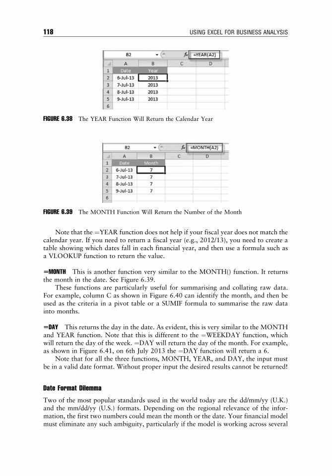
Note that the ¼YEAR function does not help if your fiscal year does not match thecalendar year. If you need to return a fiscal year (e.g., 2012/13), you need to create atable showing which dates fall in each financial year, and then use a formula such asa VLOOKUP function to return the value.

5MONTH This is another function very similar to the MONTH() function. It returnsthe month in the date. See Figure 6.39.

These functions are particularly useful for summarising and collating raw data.For example, column C as shown in Figure 6.40 can identify the month, and then beused as the criteria in a pivot table or a SUMIF formula to summarise the raw datainto months.

5DAY This returns the day in the date. As evident, this is very similar to the MONTHand YEAR function. Note that this is different to the ¼WEEKDAY function, whichwill return the day of the week. ¼DAY will return the day of the month. For example,as shown in Figure 6.41, on 6th July 2013 the ¼DAY function will return a 6.

Note that for all the three functions, MONTH, YEAR, and DAY, the input mustbe in a valid date format. Without proper input the desired results cannot be returned!

Date Format Dilemma

Two of the most popular standards used in the world today are the dd/mm/yy (U.K.)and the mm/dd/yy (U.S.) formats. Depending on the regional relevance of the infor-mation, the first two numbers could mean the month or the date. Your financial modelmust eliminate any such ambiguity, particularly if the model is working across several

FIGURE 6.38 The YEAR Function Will Return the Calendar Year

FIGURE 6.39 The MONTH Function Will Return the Number of the Month

c06 22 June 2012; 18:32:48


different regions. It is therefore best practice to format date as 5-June-2014 insteadof 5/6/14. This way there is no chance of it being interpreted erroneously as 6thMay 2014!

Long and Short Date Formatting A shortcut exists on the Home tab that allows you tovery quickly change the date format on any cell from the Number ribbon, as shown inFigure 6.42.

In the drop-down menu you should see both the options Short Date and LongDate. The samples for both are shown in the drop-down itself for easy understanding.While you could use any format in your calculations, you can eliminate confusion bysticking to long date format for any information that requires user interaction. SeeFigure 6.43.

The short and long dates are not the only formats that Excel provides; you canchoose from a much wider range of formats by clicking on the dialog box launcher inthe Number ribbon as shown in Figure 6.44.

FIGURE 6.40 Using a MONTH Function in a Report that Can Then Be Summarised

FIGURE 6.41 Using a DAY Function to Return the Calendar Day of the Month

c06 22 June 2012; 18:32:48


This brings up the Format Cells dialog box, which you can use to change the waythe date appears. In Excel for Mac 2011, the Format Cells dialog box can be found byselecting Format—Cells from the toolbar.

In all versions of Excel, the Format Cells dialog box can be found by right-clickingon the cell and selecting Format Cells.

See the section on “Custom Formatting” in Chapter 7 for more detail on how tocreate different formats.

FIGURE 6.42 Shortcut to Date Formatting in Excel 2007 and 2010

FIGURE 6.43 Shortcut Date Formatting Drop-Down in Excel 2007 and 2010

FIGURE 6.44 Formatting Dialog Box Launcher in Excel 2007 and 2010

c06 22 June 2012; 18:32:48


TIP

When you drag a series of dates in Excel, it will auto fill it for you. If you want to excludethe weekends in your financial model, Excel can do it automatically for you with theAuto Fill options. Select Fill Weekdays to exclude weekends. See Figure 6.45.

FINANCIAL PROJECT EVALUATION FUNCTIONS

Financial functions are designed to save Excel users time when calculating long andcomplicated formulas such as interest repayments, depreciation, or net present values(NPVs). They can be created manually, and if you have studied business or finance atthe university level, you will have had to create these calculations the long way or usinga financial calculator. The pre-defined function in Excel saves time and makes it mucheasier to calculate commonly used financial calculations.

There are three financial functions that are commonly used to assess a business caseor any series of cash flows: NPV, internal rate of return (IRR), and payback period.There are pre-defined functions in Excel for calculating NPV and IRR, but there is notone for payback period. For methods on how to calculate it, see the section on “How toCalculate a Payback Period” in Chapter 9.

NPV (Net Present Value)

NPV is the value of the expected future cash flows from an investment, expressed intoday’s dollars. The investor specifies a target rate of return (the cost of capital) forinvesting capital; it is an opportunity cost concept. Investors have the choice ofinvesting in a project, or putting their funds elsewhere, so they determine the hurdlerate, or the amount they want to get back from the project.

FIGURE 6.45 Auto Fill Option

c06 22 June 2012; 18:32:48


The general rule (and the one you would have studied in your university financetextbooks) for considering the investment is: If the NPV is greater than zero, theinvestment should be accepted; if the NPV is negative, it should be rejected. A positiveNPV means the investor can expect to earn a rate of return greater than the requiredreturn rate for such an investment. However, from a financial modelling perspective,the decision-making process is much more complicated than a deal-or-no-dealsituation. It really depends on the scenario and sensitivity analysis from the financialmodel to test whether or not the project should go ahead. Large companies often havepolicies regarding the standard cost of capital or how long the payback period can bebefore it is rejected.

What Cost of Capital Should We Use? How much time is spent calculating the cost ofcapital really depends on how detailed your modelling is. Many models will simply usea nominated amount and document this as an assumption. This nominated cost ofcapital could be anything between, say, 6 and 15 percent (although sometimes higher),and it can fluctuate depending on the perceived risk of the project. We may decideto use very high required rate of return for a risky project to compensate for therisk taken.

However, instead of simply nominating a cost of capital amount as we will do inthe example in Figure 6.46, you may decide to calculate the weighted average cost ofcapital (WACC). This calculation takes into account the mixture and rates of debt andequity in the company, and is therefore a much more accurate way of evaluating theexpected rate of return for a project. For more detail on how to calculate the WACC,see the section on “Weighted Average Cost of Capital (WACC)” in Chapter 9.

What Is Wrong with the NPV Function? Note that a key assumption of the NPV function isthat the cash flows occur at the end of the period, whereas in reality they will probablyoccur unevenly throughout the year, with a large portion of costs spent closer to thebeginning of the period. In this example we have included the initial investment inthe first year. If, however, we know that a large initial investment will be made priorto the start of the project, then this should be included in Year 0, and added to theNPV calculation like this: 5NPV(B4,B2:F2)1Y0_investment.

IRR (Internal Rate of Return)

IRR equates the present value of the cash inflows and the present value of the cashoutflows. The decision rule in this case is: If the IRR is greater than or equal to theinvestor’s required rate of return, the investment should be accepted; otherwise itshould be rejected.

Comparing IRR with the Risk Factor Knowing about the IRR is of little use unless you canmake decisions using it. To do that, you must compare the IRR with the risk factor.

There are two possible outcomes when you compare IRR with the risk.

1. The projected returns from the investment are greater than the risk. In otherwords, the returns from the investment are high enough to justify the risk of theinvestment. This is a positive recommendation to invest.

c06 22 June 2012; 18:32:49


2. The projected returns from the investment are less than the risk. In other words,the returns from the investment are not high enough to justify the risk of theinvestment. This is a negative recommendation, cautioning against investment.

Like NPV, IRR uses all three criteria—returns, risk, and time—in its evaluation, andfor this reason, many managers find it an easy, accurate, and dependable tool to use.

Using NPV and IRR to Make Decisions Just because the NPV is positive, and our IRR isgreater than our required rate of return, does not necessarily mean that we should goahead with the project! Blindly accepting the output of a model is a dangerous business.As we know, a model is only as good as the assumptions that go into it, and if we haveincluded aggressively optimistic assumptions in our model, of course the NPV will lookgood—but this does not mean the project will do well!

All financial models should be subjected to, at minimum, a base case, best case, andworst case scenario, which are used to evaluate the sensitivity of outputs to changes ininputs. The NPV, IRR, and payback period, which are calculated by the model, should

HOW TO CALCULATE THE NPV

With a series of cash flows as shown in Figure 6.46, the NPV is calculated asfollows.

1. Select NPV function. At the Rate prompt, enter the cost of capital, which wewill assume is 12 percent.

2. At the Value1 prompt, link the formula to the cells that contain the expectedreturn (i.e., as we are calculating the five-year NPV, it will be the profit orloss for 2013 to 2017). The formula should be 5NPV(B4,B2:F2).

3. The result of your formula should be $127,568.

In this case, the NPV is greater than zero, meaning that the return is greaterthan the required rate of return of 12 percent stated by the company. This meansthat, theoretically, the project should be accepted. However, scenario and sen-sitivity analysis will help determine how sensitive the model is to changes ininputs and gain a better perspective on whether or not this project should beaccepted.

FIGURE 6.46 Using the NPV Function

c06 22 June 2012; 18:32:49


be used as decision-making factors and not the ultimate deciding factors of the fate ofthe project.

The Problem with IRR There are a few problems with the IRR function that the modellerneeds to be aware of.

Sometimes the IRR function in Excel can produce multiple results. Every time thecash flows change sign (i.e., from negative to positive or from positive to negative),the formula will create another solution. This is why it a good idea to insert a guessamount—especially if the sign of the cash flows is not consistent.

Take the following set of cash flows in Figure 6.48 as an example.If we use the ordinary IRR function without using the guess [entered as 5IRR(B2:

H2)], we get a result of 13 percent. However, because there are several negative returns

HOW TO CALCULATE THE IRR

Using the same investment assumptions as in the previous example, the rate ofreturn on the initial investment can be calculated as follows:

1. Select the IRR function.

2. At the Values prompt, select or specify the cells that contain the requestedinformation.

3. Leave the Guess prompt blank at this stage. (See the forthcoming section on“The Problem with IRR” for more detail on when and why you need toinclude a guess.) In this instance all the cash flows are positive, so we don’tneed to enter a guess.

4. Click on the OK button and the yield (IRR) is displayed. The formula shouldbe: ¼IRR(B2:F2).

The result of your formula should be 13.3 percent and look somethinglike Figure 6.47.

In this case, the IRR is higher than the required rate of return of 12 percent,as stated by the company. This means that, theoretically, the project should beaccepted.

FIGURE 6.47 Using the IRR Function

c06 22 June 2012; 18:32:49


in this series of cash flows, there are multiple results. If you enter the following guesses,different IRRs will be returned:

n ¼IRR(B2:H2) gives a result of 13 percent.n ¼IRR(B2:H2,0) gives a result of 6 percent.n ¼IRR(B2:H2,30%) gives a result of 25 percent.n ¼IRR(B2:H2,400%) gives a result of 481 percent.

Which one is correct? They all are! There are as many valid IRRs as there arechanges in sign. Excel goes through an iterative process and comes up with the firstsolution it finds, which does not necessary give you result you want. This is why it’simportant to use the guess. If the guess is omitted, IRR is assumed to be 10 percentbecause this is close to a usual rate of return.

Another issue with the IRR is that the way the IRR function calculates in Excel, itassumes that cash generated during the investment period will be reinvested at the ratethat has been calculated by the IRR. If the project is generating a lot of cash, the IRRcalculation can overstate the financial benefits substantially, which is something thatneeds to be considered, and possibly manually manipulated in the calculations.

We don’t normally make any changes to the calculations to account for theseproblems, but it’s important to consider these issues when calculating the IRR.

What Difference Does an X Make? XNPV and XIRR

The NPV formula assumes that the values entered into the formula are annual, are inchronological order, and occur at the end of the period

The XNPV formula offers more flexibility, as you can specify exactly when thepayments occur. However, XNPV and XIRR are only available in Excel 2007 and later.

XNPV allows you to enter payments that occur at varying intervals, not necessarilyin chronological order (although the first payment must still be shown first), and occurat any time. Therefore, it is a much more flexible and useful function. Also, because itdoes not assume that the payments occur at the end of the period, the XNPV formulawill be more accurate.

Be careful when comparing the NPV and XNPV functions, as the NPV assumes thecurrent period (the date we are in right now) is a full year prior to the first cash amountand therefore discounts the first amount back by a full 12 percent (or whatever thenominated discount rate is). If this is not the case, you need to exclude the first periodfrom the function, and add it in separately, like this:5NPV(B4,B2:F2)1Y0_investment.

The XNPV function, however, assumes that the current date is the date of the firstcash flow, so in the example above, the current date is assumed to be 1st June 2013.Therefore, the first cash amount is not discounted at all. IRR and XIRR have the

FIGURE 6.48 IRR Calculation with Multiple Results

c06 22 June 2012; 18:32:49


same issue. This is quite misleading, as most people naturally assume that the functions,being slight variations on the same formula, work in a similar way, but the way theytreat the first cash amount is quite different!

LOAN CALCULATIONS

Calculating debt is an important part of many financial models, and understanding thetheory behind how loan repayments are calculated will help in financial modelling.The way that interest, principal, and periodic payments are calculated can be com-plicated, and fortunately for us, Excel has many useful functions that make calculatingloans a lot easier. However, you should still have a basic understanding of how loancalculations work!

Loan-Interest Calculation Method

Interest on loans can be calculated using either the simple interest method, or the com-pound interest method. The simple interest method charges the same amount of interesteach year, but under the compound interest method, the interest is added to the loan, so

HOW TO CALCULATE THE NPV USING THE XNPV FUNCTION

If you were to be more precise about the actual timings of the expected cash flow,you would get a more accurate NPV calculation using XNPV.

Instead of saying that you expect a net outflow of $3.2 million in 2013, let’s bea little more specific about when the outflows actually occur. Let’s say you splitthat into $2 million in June 2013, and the rest at the end of the year. We will alsoput a date in the middle of the year for subsequent years, which is more likelyto accurately reflect whatwill happen, instead of assuming that payments aremadeor received at the end of the period, as it does with the NPV calculation.

Figure 6.49 shows the cash flows.

Using the XNPV formula, and assuming that the cost of capital is, say, 12percent, the formula should be 5XNPV(B4,B2:G2,B1:G1), giving us a result of$190,828.

Similarly, theXIRR can be calculated using the formula5XIRR(B2:G2,B1:G1)giving us a result of 13.8 percent.

FIGURE 6.49 XNPV Function

c06 22 June 2012; 18:32:50


increasing the loan amount each year. From the moment at which the interest is addedto the loan, it charges interest on itself, increasing the interest on a compoundingbasis. The compound interest method is by far the most commonly used method, and inthe examples in this chapter we assume that the interest is compounding.

When evaluating a loan, you may also need to consider the compounding fre-quency. If the interest is added to the loan on a daily basis, this would actually make theloan interest payments much higher than if it were added monthly or annually. Mostloans are normally calculated on a daily basis, and this means the interest rate actuallycharged is higher.

Note that the PMT function shown below, if calculated on an annual basis, doesnot compound the interest. You will need to convert the interest rate from a nominal oreffective rate before using in the calculation.

Nominal and Effective Interest Rates

Weare used to seeing interest rates expressed as an annual rate (e.g., an interest rate of 12percent means that we are charged 12 percent per year). However, this is onlythe nominal rate, and this does notmean thatwe are charged 1 percent permonth. In fact,if the interest is calculated daily, we are charged 12 percent divided by 365, or 0.33percent on the first day of the loan. This amount is added to the principal, so on day two,we are actually paying interest on the interest from the previous day. I know this soundstrivial but it can make a big difference to your calculations on a large debt.

TIP

An easy way to work out the effective interest rate is to use the EFFECT function (onlyavailable in Excel 2007/10) to calculate the effective rate of 12 percent, compoundeddaily. Use the formula ¼EFFECT(12%,365). The answer is 12.75 percent. See thesection on “Understanding Nominal and Effective (Real) Rates” in Chapter 9 for moredetail on how to use this function as well as the NOMINAL function. Note that theEFFECT function is not available in standard Excel 2003.

Loan Repayment According to an Amortisation Schedule

The most common form of calculating loan repayments is to apply an amortisationschedule. Regular repayments of equal value made over the term of the loan are used topay both the interest charged as well as a portion of the principal amount. With eachrepayment, an amount equal to the value of the interest charged for the period isapplied first to the interest portion, and the remainder of the repayment is then set offagainst the principal. In this way, the principal decreases after each repayment and theinterest calculated for the next period will therefore be less, as it is calculated on asmaller principal amount.

To calculate the amount of the equal repayments to be made, the interest rate, theprincipal amount, and the term of the loan must be known. As interest rates are usuallysubject to change, the monthly repayment will often have to be revised during thecourse of the loan.

c06 22 June 2012; 18:32:50


If you need to calculate the repayments long-hand using the amortisation method,the following formula is used:

repayment ¼ loan amount3 ið1þ iÞnð1þ iÞn � 1

� �

where i¼ the interest rate per annum, which must be divided by the number of repay-ment periods per annum (e.g., 12 periods if payments are made monthly).

n¼ the number of repayment periods (e.g., 24 if the loan is for a period of 2years and repayments are made monthly).

Excel Amortisation Functions Whilst it’s good to know the theory of how the repaymentsare calculated, fortunately Excel offers several loan calculation functions that can beeasily included in financial models. The following are some of the most commonfunctions available in Excel for loan-related calculation.

PMT This is the very basic function that calculates the fixed amount you need to payat regular intervals to repay the loan along with fixed interest. This is the syntax forusing the PMT function: PMT (rate, number of payments, principal amount, finalamount, type). In this syntax, the following applies:

n Rate: This is the fixed interest rate for the loan period.n Number of Repayments: This is the number of instalments within which you want

to repay the loan.n Principal Amount: Amount of original loan (no interest included).n Final Amount: The total amount at the end of all the instalments. This is not a

mandatory field and the default value is set to zero.n Type: This determines when the payment needs to be made. The default value is

zero, which means at the end of the period; one means at the start of the period.

In Figure 6.50, we have a loan of one million dollars repaid over a 10-year period(annually) at an 8 percent interest rate. The PMT function calculates the fixed paymentamount, which in this case is $149,029.

FIGURE 6.50 PMT Function

c06 22 June 2012; 18:32:50


IPMT The IPMT function is complementary to the PMT function. While PMTcalculates the entire repayment instalment amount, IPMT gives the interest componentof the instalment. Like the PMT, this is calculated for fixed principal and interest ratefor a given duration of time. The syntax for IPMT is IPMT (rate, period, number ofpayments, principal amount, final amount, type), where the following applies:

n Rate: This is the fixed interest rate for the loan period.n Period: This is the period for which the interest amount needs to be calculated. For

the first period (week, month, year, etc.) this would be 1, and for subsequentperiods it will increase as 2, 3, 4, and so on.

n Number of Repayments: This is the number of instalments within which you wantto repay the loan.

n Principal Amount: Amount of original loan (no interest included).n Final Amount: The total amount at the end of all the instalments. This is not a

mandatory field and the default value is set to zero.n Type: This determines when the payment needs to be made. The default value

is zero, which means at the end of the period; one means at the start of theperiod.

In Figure 6.51, C10 represents the period that changes in the formula, while allother parameters are fixed references to the loan amount.

PPMT This is another complementary function to the PMT function. Like theIPMT, PPMT returns the other component of the instalment: principal amount.

The syntax for PPMT is PPMT(rate, period, number of payments, principalamount, final amount, type). In this syntax, the following applies:

n Rate: This is the fixed interest rate for the loan period.n Period: This is the period for which the interest amount needs to be calculated. For

the first period (week, month, year, etc.) this would be 1, and for subsequentperiods it will increase as 2, 3, 4, and so on.

n Number of Repayments: This is the number of instalments within which you wantto repay the loan.

FIGURE 6.51 IPMT Function

c06 22 June 2012; 18:32:50


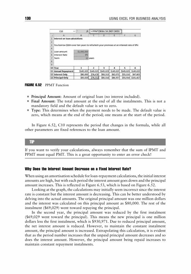
n Principal Amount: Amount of original loan (no interest included).n Final Amount: The total amount at the end of all the instalments. This is not a

mandatory field and the default value is set to zero.n Type: This determines when the payment needs to be made. The default value is

zero, which means at the end of the period; one means at the start of the period.

In Figure 6.52, C10 represents the period that changes in the formula, while allother parameters are fixed references to the loan amount.

TIP

If you want to verify your calculations, always remember that the sum of IPMT andPPMT must equal PMT. This is a great opportunity to enter an error check!

Why Does the Interest Amount Decrease on a Fixed Interest Rate?

Whenusing an amortisation schedule for loan-repayment calculations, the initial interestamounts are high, but with each period the interest amount goes down and the principalamount increases. This is reflected in Figure 6.53, which is based on Figure 6.52.

Looking at the graph, the calculations may initially seem incorrect since the interestrate is constant but the interest amount is decreasing. This can be better understood bydelving into the actual amounts. The original principal amount was one million dollarsand the interest was calculated on this principal amount as $80,000. The rest of theinstalment ($69,029) went toward repaying the principal.

In the second year, the principal amount was reduced by the first instalment($69,029 went toward the principal). This means the new principal is one milliondollars less the first instalment, which is $930,971. Due to reduced principal amount,the net interest amount is reduced. However, to maintain the constant instalmentamount, the principal amount is increased. Extrapolating this calculation, it is evidentthat as the period number increases that the unpaid principal amount decreases and sodoes the interest amount. However, the principal amount being repaid increases tomaintain constant repayment instalments.

FIGURE 6.52 PPMT Function

c06 22 June 2012; 18:32:51


SUMMARY

In this chapter we have covered a couple of the important aggregation, lookup,referencing, date, and finance functions that, at minimum, are important for afinancial modeller to know. As we know, however, there is a lot more to being agood financial modeller than knowing hundreds of different Excel functions! Themost challenging part is to knowwhen to use these functions in your modelling. Whenfaced with a problem, creating a modelling solution that contains the most appro-priate tools and functions is the task faced by the financial modeller. Usually, there areseveral different possible tools that can be used, and the one that is the most concise,yet easiest to follow will be the best solution.

$160,000Loan Repayments over Ten Years

$140,000

$120,000

$100,000

$80,000

$60,000

$40,000

$20,000

$69,029

$80,000

$74,552

$74,478

$80,516

$68,513

$86,957

$62,072

$93,914

$55,116

$101,42

$47,603

$109,54

$39,488

$118,30

$30,725

$127,76

$21,261

$137,99

$11,039

$01

Principal Only

Interest Only

2 3 4 5 6 7 8 9 10

FIGURE 6.53 Principal (PPMT) and Interest (IPMT) Components of Loan Repayments Over TenYears

c06 22 June 2012; 18:32:51


c06 22 June 2012; 18:32:51

CHAPTER 7Tools for Model Display

Leaving aside the formulas and calculations of a model, in this chapter we will focuson the look and feel of a model. There are many Excel tools that can be used to make

the model more attractive and friendly to the user. We’ll look at the basic formatting,and then more complex custom formatting, conditional formatting, and then formcontrols, which can be built to help the user interact with the model more easily.

BASIC FORMATTING

Believe it or not, as simple as it may sound, good formatting is an important part ofbuilding a financial model. While it’s critical of course to get the numbers right, makingyour model look good is the next step! A model that is well formatted will be morereadable, user-friendly, and easy to navigate. Additionally you, the modeller, will findit easier to work with the model if it is clearly formatted.

In the latest version of Excel, all the formatting options for colour, font, andalignment are clearly displayed on the Home tab. A shortcut exists on the Home tabwhere you can very quickly change the number format on any cell from the Numberribbon, as shown in Figure 7.1.

For detailed instructions on the more basic formatting tools, including changingnumber formats, percentage and currency formatting, number alignment, cell attri-butes, and styles, please see the supplementary material at www.wiley.com/go/steinfairhurst, available for download in PDF format. The instructions for Excel 2003 canbe found in the Excel 2003 supplementary document.

CUSTOM FORMATTING

We can go one step further with our formatting to customise the way data is displayedin cells without changing the underlying data. For instance, the function 5NOW() gets

FIGURE 7.1 Formatting from the Ribbon in Excel 2010

c07 23 June 2012; 12:17:24

133



the current date and time from your computer and, by default, displays it in the format“dd/mm/yyyy hh:mm” (or according to the date conventions in your computer’sRegional and Language Options within Control Panel).

We can change the look of this date without disturbing its intrinsic value by for-matting it differently. Let’s have a look at how we’d do this:

1. Open a blank spreadsheet and type into cell A1 Report as at, and into cell B1 typethe function 5NOW() or 5TODAY().

2. Size the column widths to match the data, then select cell B1 for formatting. SeeFigure 7.2.

3. Choose Format on the Cells section of the Home tab. Select Format Cells at thebottom of the drop-down list that appears.

In Excel for Mac 2011, from the Format menu, select Cells.The dialog box in Figure 7.3 appears, showing how Excel has already cus-

tomised the cell.

FIGURE 7.2 Showing the Current Date and Time Using the ¼NOW() Function

FIGURE 7.3 Format Cells Dialog Box

c07 23 June 2012; 12:17:24


As can be seen from the dialog box, there are many pre-set formatting optionsfor numbers, from General to Accounting to Custom. As suggested within thedialog box, we can type our own codes over pre-set ones if the format we wantisn’t available.

4. To create a customised format, select Custom from the Category list. OverwriteExcel’s choice of “dd/mm/yyyy hh:mm” with just the three characters “mmm” andobserve what Excel does with your date. Add a further “m” to make our customformatting “mmmm” and the result will be, after reflection, obvious.

5. Custom format your current date to the following format: 24 Feb 2014 (your datewill be different in content).

In all Windows Excel versions, the shortcut key Control þ 1 will invoke the for-matting dialog box as seen in step 3, above. For Excel for Mac 2011, pressCommand þ 1.

Excel 2010 has an additional shortcut to pre-set formats in the Number section ofthe Home tab, as seen in Figure 7.4.

Excel for Mac 2011 has the most commonly used formats pre-set on the For-matting toolbar; namely currency, percent, thousands separator, and decimal places,but dates are not there. You’ll need to use the Format Cells dialog box to format cells todates.

FIGURE 7.4 Changing the Date Format

c07 23 June 2012; 12:17:25

Tools for Model Display 135

Custom Currency Symbols

As mentioned earlier, changing the look of a cell doesn’t affect the underlying data. Sofar we’ve played with dates (which are numbers to Excel even though they’re generallydisplayed as text), but there are plenty of other pre-set number formats that we can, ifnecessary, customise.

1. Go to a blank sheet, and type in 582504 into a cell. If you have not defined anyformatting on that cell yet, Excel will assign a General format to it.

2. Change the number to currency (to two decimal places) preceded by your country’smonetary symbol, by using the Currency category in the Format Cells dialog box.

3. Change the currency symbol to that of the Chinese Yuan, or some other foreigncurrency.

4. Change the currency symbol to that of a currency we’ve made up—Elbonian Spree(EL).

As you might have suspected, the Elbonian Spree isn’t available in the list ofsymbols. We’ll have to build a custom format for it.

Select the Custom category and overwrite Excel’s f symbol with EL, asfollows:

[$f-804]#,##0.00;[$f-804]-#,##0.00 is changed to "EL" #,##0.00;-"EL" #,##0.00

Note that EL, as invented by us, is unknown to Excel and must be presented asa string (i.e., in quotes). This custom currency symbol will be saved with theworkbook and will be available for future use.

Understanding Excel’s Number Formats

Number formats have four elements:

1. Positive number2. Negative number3. Zero4. Text

Each is separated by a semicolon. None of them are mandatory, but there shouldbe a positive element, at least.

Consider the elements in the format $ * #,##0; [Red]$ * -#,##0; $ * "�";"*"

Positive Negative Zero Text

Format $ * #,##0 ; [Red]$ * �#,##0 ; $ * "�" ; "*"Value 1000.00 �100.00 0.00 JackRepresentation $ 1,000 $ �100 $ � *

Leading zeros of both positive and negative numbers will be suppressed wherever #is specified. Negatives will show the minus symbol after $ and zeros will display �. Thetext Jack will be represented as a single asterisk. The monetary symbol asterisks ($ *)

c07 23 June 2012; 12:17:25


indicate that the symbol must be fixed to the left and not follow the number as itshrinks or expands.

You’ll note that Excel sometimes uses codes, particularly in currency formats.These are used, for instance, in differentiating between Australian and U.S. dollars, andneedn’t concern us.

The important thing to remember is that the underlying number doesn’t change nomatter how we format it. It retains its decimal places even if we can’t see them.Arithmetic can continue to be done on a cell’s contents, even if it’s invisible.

Useful Formatting Options

If you intentionally leave an element blank, it will be rendered invisible. ;$-#,##0.00;;will show negatives only, all the other elements being deliberately suppressed. Theentry ;;; will make everything in the cell invisible (so will changing the font colour tomatch the background).

To display a number as 000s, while still retaining its full value, custom format itas $#,##0, (the format followed by a comma). Millions are represented by $#,##0,,“m”. $458,243,555.42 will display as $458m, which, if multiplied by one, will return$458,243,555.42. If this does not work, your digit grouping symbols within Regionaland Language Options in the Control Panel are not set as commas.

Tophysically change a number to rounded thousands use theROUND,ROUNDUP,or ROUNDDOWN functions, employing minus digits. ROUND(458243,-3) willchange the number to $458,000. The format $#,##0, will display $458, which, ifmultiplied by one will return $458,000.

To make currency negatives by default show in parentheses, change your negativeCurrency Format options within Regional and Language Options in the Control Panelto default to parentheses.

Custom Formatting in Reporting

Create some numbers that look like Figure 7.5:

FIGURE 7.5 Sample Report

c07 23 June 2012; 12:17:25


We are going to format the numbers so that they look similar to Figure 7.6(without changing the underlying data):

1. Highlight the data and, as described above, go to the Custom Formatting dialogbox.

2. Add a comma to the end of the format type as shown in Figure 7.7.

This will change the look of the numbers without changing the value of thenumbers at all.

FIGURE 7.6 Completed Report

FIGURE 7.7 Custom Formatting Using the Format Cells Dialog Box

c07 23 June 2012; 12:17:25


Next, add up cells B4:B8 manually. You’ll notice that the total should be $1,612,not $1,611! Use the ¼ROUND formula, as shown above, to round the numbers to thenearest thousand, such that your report or PowerPoint slide is correct.

CONDITIONAL FORMATTING

Conditional Formatting is a tool that allows you to apply formats to a cell or range ofcells, and have that formatting change, depending on the value of the cell or the valueof a formula. For example, you can have a cell appear bold only when the value ofthe cell is greater than 100. When the value of the cell meets the format condition, theformat you select is applied to the cell. If the value of the cell does not meet the formatcondition, the cell’s default formatting is used.

This is handy for variance analysis on a profit and loss (P&L), for example. If youwant to highlight any instance where a variance is greater than 10 percent higher thanbudget, the cell will turn red.

Remember that Conditional Formatting is the same as adding one or more for-mulas to each cell in which you use it, so applying Conditional Formatting to a largenumber of cells may cause performance degradations. Use caution when applying tolarge ranges!

Conditional Formatting is greatly improved in Excel 2007/10. There are manymore options (including the handy Data Bars), and the limitation of three conditionshas been lifted. (See the Excel 2003 instructions available at www.wiley.com/go/steinfairhurst.)

To Apply Conditional Formatting

1. Select the desired cell or cells in the spreadsheet. Let’s say, for example, youwanted to highlight with a red font any cell value that is between 1 and 10.

2. On the Home tab, in the Styles group, select Conditional Formatting. SelectHighlight Cells Rule and then Between. Type in 1 and 10, and define the desiredfont colour. See Figure 7.8.

Add a new rule for each new condition; you can have as many as you like (unlike inExcel 2003, where you are limited to three rules).

To Remove Conditional Formatting

On the Home tab, in the Styles group, select Conditional Formatting. Select ManageRules, and you can delete your chosen rules one by one. Alternatively, you can clearrules from selected cells or from the entire sheet by clicking on Clear Rules.

Data Bars

Data bars are a new feature in Excel 2007 and, therefore, it is possible to create them inversions 2007, 2010, and Excel for Mac 2011, but not in Excel 2003. Data bars are adynamic bar chart that you can apply to any numerical data in Excel. They graphicallyshow the relative size of each value. See Figure 7.9.

c07 23 June 2012; 12:17:26




Go to a table of numeric data, and highlight the numbers.

1. On the Home tab, in the Styles group, select Conditional Formatting, and thenData Bars.

2. Choose your desired bar.3. Practice changing the underlying numbers, and see the bars change.

Icon Sets and Colour Scales

Icon Sets are a feature that was new to Excel 2007. They allow you to conditionallydisplay a small icon that represents changes in data. For example, if revenues are downthis month compared to last, you may choose to represent this with a red arrowpointing down, or if your cash balance is above a certain threshold, you could use agreen checkmark to give the user a quick way to see that everything is okay.

FIGURE 7.9 Data Bars in Excel 2010

FIGURE 7.8 Conditional Formatting in Excel 2007/10

c07 23 June 2012; 12:17:26


Your options for icons currently available in Excel 2007/10 are shown in Figure7.10. Note that there is no way to import any additional icons, but this might bepossible in future releases.

Another feature new to Excel 2007 was Colour Scales. Looking at Figure 7.11,how would you be able to quickly assess what is good, bad, and in-between?

By using Colour Scales, you can assign rules for what is good, bad, and in-between,and display the data with colour to represent these rules. You can see in Figure 7.12how data is more useful when the user can quickly spot areas of concern.

Enhancements to Conditional Formatting in Excel 2010

You have access to more icon sets, including triangles, stars, and boxes. You can alsomore easily hide icons from view, as is evident in Figure 7.13.

Being able to hide the icons is a new feature applicable to Excel 2010 and Excel forMac 2011 only.

FIGURE 7.10 Accessing Icon Sets

FIGURE 7.11 Sample Report

c07 23 June 2012; 12:17:26


Editing the rule gives you a variety of options. See Figure 7.14.You can also easily mix and match data bars, colour scales, and icons from dif-

ferent sets. In Figure 7.15 the same range has both data bars and icons.The automatic negative bars as shown in Figure 7.15 are a new feature, available in

Excel 2010 and Excel for Mac 2011 only.In Excel 2010 and Excel for Mac 2011, you can also create conditional for-

matting with references to a different sheet in the workbook. This means that you nolonger need to copy or link your data to the same sheet when using conditionalformatting.

FIGURE 7.13 Hiding Icons in Excel 2010

FIGURE 7.12 Sample Report Using Colour Scales

c07 23 June 2012; 12:17:26


SPARKLINES

Just like Conditional Formatting and the Icon Sets, Excel also has another interestingmicro-charting feature termed the sparkline. These lines are not as descriptive as reg-ular graphs and charts, but they are very effective in displaying a quick view about thetrends in the data or metrics. This is a new feature introduced in Excel 2010, so it is anenhancement over the older versions. At the same time, since this is the first release, thedesign is not necessarily as polished as a modeller would hope. Note that sparklines canonly be created and viewed in Excel 2010, so if your model is viewed in Excel 2007 orearlier, the sparklines will disappear. This is one of the few instances where Excel 2007and 2010 differ in functionality.

FIGURE 7.14 Editing Icon Set Rules in Excel 2010

FIGURE 7.15 Applying Multiple Types of Conditional Formatting to a Single Cell

c07 23 June 2012; 12:17:27


HOW TO CREATE A SPARKLINE

1. Select the data series for which the sparkline needs to be created. See Figure7.16.

FIGURE 7.16 Data to Contain Sparklines

2. Under the Insert tab in the Sparklines ribbon, select Line. Note that spark-lines are found in the Charts ribbon under Insert Sparklines in Excel for Mac2011. See Figure 7.17.

FIGURE 7.17 Choosing Sparklines from the Ribbon

3. In the Create Sparklines dialog box, the data range is automatically selected,so enter the cell or cell range in which you want the sparklines to be placed.Click OK. See Figure 7.18.

FIGURE 7.18 Sparklines Dialog Box

4. The sparklines are drawn in the selected cells. See Figure 7.19.

FIGURE 7.19 Completed Report with Sparklines

c07 23 June 2012; 12:17:27


TIP

Use a combination of sparklines and icons to create more meaningful representationsof data points.

Editing Sparklines

The attributes of the sparklines can be modified from options under the Design tab. Toedit data, select the sparklines and click on the Edit Data in Sparkline ribbon under theDesign tab. See Figure 7.20.

This will open the Edit Sparklines dialog box, where you can change the data rangeas well as the sparkline location. See Figure 7.21.

To edit chart type, select the sparklines and click on one of the three options in theType ribbon under the Design tab. See Figure 7.22. The three options are:

FIGURE 7.20 Editing Sparklines

FIGURE 7.21 Edit Sparklines Dialog Box

FIGURE 7.22 Changing Sparkline Type on the Ribbon

c07 23 June 2012; 12:17:27


n Line: Simple line graph.n Column: Column graph, similar to area plots.n Win/Loss: Map the data in win/loss format.

To highlight important points in the sparklines, choose from:

n High Pointn Low Pointn Negative Pointsn First Pointn Last Point

To highlight important data points, select from a series of checkboxes in the Showribbon, under the Design tab. See Figure 7.23.

You can also edit the style of the sparklines by changing the line colours andmarker colours. See Figure 7.24.

Changing Properties for a Group of Sparklines

While each sparkline represents a unique series of data, you can edit the properties of agroup of sparklines using the group and ungroup features. When the sparklines aregrouped, you can edit the properties for the entire group, even if you select just a singleline from the group. See Figure 7.25.

To separate out the sparklines in the group, select Ungroup in the Group ribbonunder the Design tab.

TIP

If you want to create a series of sparklines for a series of data points, you can create itfor the first list and just copy paste the sparkline to auto-create it for the rest of the lists.

FIGURE 7.23 Highlighting Sparkline Data Points on the Ribbon

FIGURE 7.24 Editing Sparkline Formatting on the Ribbon

c07 23 June 2012; 12:17:28


BULLETPROOFING YOUR MODEL

If your model is publicly available, or if you have a lot of users entering data into it(especially if their Excel skills are questionable), it’s a good idea to spend some timeprotecting it and making sure that all your hard work is not inadvertently corrupted!

Protection

Once you have completed building your model, there are three basic layers of pro-tection you can include:

1. Protect the file so that no one can open it without the password.2. Protect the structure of the workbook so that no structural changes can be made

(normally used for hiding sheets and restricting access to them).3. Unlock individual cells on the worksheet and then protect the sheet so that only

those cells that are unlocked can be changed.

Protecting the structure or worksheets can be done with or without a password.

WARNINGDo not use a password unless you are certain that you will not forget what it is! There is no wayto retrieve a forgotten password in Excel. Passwords are case-sensitive.

However, if it is a matter of life and death, do not trust your model to a password! Pass-words can be hacked reasonably easily. Note that there are programs out there that can decode apassword. If your file contains highly sensitive information, do not rely on passwords in Excel.

Protect the File

This is done by changing the options, and saving over the existing copy of the file.There are two options with this: protecting the file with a password, or recommendingread-only access.

Password-Protect a File If you don’t want anyone to be able to open your file without apassword, or make changes without a password, this is done under General Options.You can select Password to Open or Password to Modify.

FIGURE 7.25 Grouping Sparklines Together

c07 23 June 2012; 12:17:28


This is recommended if you are e-mailing a confidential file and are concerned thatit might be intercepted or viewed by the wrong person!

Read-Only Recommended Instead of using a password to prevent access, you could usethe read-only option to deter users from changing your workbooks. This way youprevent inadvertent changes to models.

Protect the Structure

The most common use of protecting the structure is to protect hidden sheets, but it alsostops users from adding or deleting sheets, or changing other structural aspects of yourmodel, but not from editing cell contents. If you want to stop users from entering dataor changing values in cells, you need to protect the worksheet. See the next section forhow to do this.

Protecting Hidden Sheets If you have a sheet containing sensitive data, you can hide theentire sheet, and then protect the workbook so that the sheet cannot be viewed. This isparticularly handy if, for example, you have salary data on sheet in a budget model anddon’t want all users to have access to the information.

Protect the Worksheet

This is the most commonly used form of protection. If you have created a spreadsheetthat you do not want to be altered by the others who might view it, you can protect thesheet. You can either protect the whole sheet, or just certain key cells in the sheet(probably those containing the formulas) so that new data can still be entered ontothe sheet.

HOW TO ENABLE READ-ONLY

1. Follow the instructions as above (“How to Password-Protect a File”).

2. Instead of typing a password, tick the Read-Only Recommended tick box.

HOW TO PASSWORD-PROTECT A FILE

1. Click on the Microsoft Office button or File menu in the top left-hand cornerof your screen and select Save As.

In Excel for Mac 2011, go to File—Save As.

2. Click on the Tools button and select General Options.

3. Enter the password, and save over the file.

c07 23 June 2012; 12:17:28


NOTE

If the sheet has been protected it sometimes is not possible to adjust column width. This can be veryfrustrating for the user, so make sure your columns are the correct width!

HOW TO PROTECT A WORKSHEET

1. Go to the sheet you wish to protect.

2. On the Review tab, in the Changes group, select Protect Sheet. (See the Excel2003 instructions available at www.wiley.com/go/steinfairhurst.)

In Excel for Mac 2011, on the Review tab, in the Protection group, selectSheet.

3. This will bring up the Protect Sheet dialog box, in which you can enter apassword to prevent users from unprotecting the sheet. You do not have touse a password; you can just leave the Password box empty, and this may beenough of a deterrent to prevent users from modifying your model.

4. Enter a password (if necessary) and click OK.

5. If you have entered a password, you will be asked to confirm the password.

6. Type the password again.

7. The whole sheet is now protected. Users will not be able to change thecontents of any cell. If you need to change cell contents you will need tounprotect the sheet.

HOW TO PROTECT HIDDEN SHEETS

1. Put all sensitive information on one sheet.

2. Hide the sheet. Right-click on the sheet tab name and select Hide. (See theExcel 2003 instructions available at www.wiley.com/go/steinfairhurst.)

3. Now protect the structure of the workbook so that users cannot unhidesheets.

On the Review tab, in the Changes group, select Protect Workbook andthen Protect Structure and Windows from the drop-down box.

In Excel for Mac 2011, on the Review tab, in the Protection group, selectWorkbook and then Protect Structure and Protect Windows from the drop-down box.

4. If you enter a password, users will need a password in order to view thesheet(s) you have hidden.

c07 23 June 2012; 12:17:29




Protect Data by Locking Cells By following the process outlined above to protect theworksheet, you will find that you won’t be able to make any changes at all to any cell!If you want to allow entry into certain cells, but leave part of the sheet protected(perhaps the cells containing formulas), you’ll need to unlock those cells to be editedfirst, before protecting the sheet. Make sure you turn off your protection beforeunlocking cells!

By default, every cell in a sheet has a lock applied to it. It is the lock that is activatedwhen the sheet is protected and stops people from editing cells. You need to unlockthose cells that should be changed.

HOW TO UNPROTECT A WORKSHEET

1. Select the tab name of sheet you wish to unprotect.

2. On the Review tab, in the Changes group, select Unprotect Sheet. (See theExcel 2003 instructions available at www.wiley.com/go/steinfairhurst.)

In Excel for Mac 2011, on the Review tab, in the Protection group, selectSheet.

3. If no password was originally used to protect the sheet, then the sheet willautomatically be unprotected at this point.

4. If a password has been used, the Unprotect Sheet dialog box will appear.Enter the password and click OK.

HOW TO LOCK OR UNLOCK SPECIFIC CELLS

You will need to have sheet protection turned off before you do this. Theseinstructions are the same in all versions of Excel.

1. Select the cells you wish to change.

2. Right-click and select Format Cells to bring up the Format Cells dialog box.

3. Then select the Protection tab.

4. Turn off Locked if you want users to be able to edit the selected cells once thesheet has been protected.

5. The Hidden option is used to stop users from viewing the formulas of theselected cells in the Formula Bar (once the sheet has been protected).

6. Click OK. Now when you protect the sheet, cells that are no longer lockedwill be editable.

c07 23 June 2012; 12:17:29



CUSTOMISING THE DISPLAY SETTINGS

The following is an example of a model that’s been very highly protected, and thedisplay settings have been changed so that it almost does not even look like an Excelfile. You can download a copy of this file called “Salary Sacrifice Calculator” fromwww.wiley.com/go/steinfairhurst and if you would like to unprotect it, use the pass-word plumsolutions. You will need to unprotect the sheet as well as the file structure,and how to do this is outlined in this section.

To make your model highly protected, like the model in Figure 7.26, you maychoose to change a few settings to make your model look less like an Excel sheet, andmore difficult for the user to change.

Removing Row and Column Headers

This is one of the few instances where the instructions differ slightly between Excel2010 and 2007. Click on the Microsoft Office button or the File tab in the top left-handcorner, go to Options or General Options. Under Advanced in Display Options for thisWorksheet, untick the Show Row and Column Headers box. (See the Excel 2003instructions available at www.wiley.com/go/steinfairhurst.)

In Excel for Mac 2011go to Excel, then Excel Preferences and under View, in theWindow Options section, untick the Show Row and Column Headers box.

FIGURE 7.26 Model with Customised Display Settings

c07 23 June 2012; 12:17:29




Removing Sheet Tabs

Click on the Microsoft Office button or the File tab in the top left-hand corner. Go toOptions or General Options, and under Advanced, in Display Options for thisWorksheet, untick the Show Sheet Tabs box.

In Excel for Mac 2011, go to Excel, then Excel Preferences and under View, in theWindow Options section, untick the Show Sheet Tabs box. (See the Excel 2003instructions available at www.wiley.com/go/steinfairhurst.)

Note that vertical and horizontal scroll bars can also be removed via the samemethod.

Removing the Formula Bar

Click on the Microsoft Office button or the File tab in the top left-hand corner; go toOptions or General Options and under Advanced, in Display, untick the Show FormulaBar box.

In Excel for Mac 2011, go to Excel, then Excel Preferences. Under View in theWindow Options section, untick the Show Formula Bar by Default box.

Minimising the Excel 2007/10 Ribbon

Again, the instructions differ between Excel 2007 and 2010. Note that this onlychanges the view in your Excel on your computer; it does not change the model. Henceif colleagues open up the same model and their Excel settings have the ribbon max-imised, they will see the whole ribbon.

In Excel 2010, go to the top right-hand corner of your screen and click on the littleicon. See Figure 7.27.

In Excel 2007, go to the Customise Quick Access Toolbar button in the top left-hand corner of your screen, and select Minimise the Ribbon from the menu. SeeFigure 7.28.

FIGURE 7.27 Minimising the Ribbon in Excel 2010

FIGURE 7.28 Minimising the Ribbon in Excel 2007

c07 23 June 2012; 12:17:30



TIP

You can also minimise the ribbon by simply pressing Control þ F1! (Option þCommand þ R in Excel for Mac 2011).

Restrict the Work Area

You can make the work area of the sheet much smaller so that users cannot enter datain cells you don’t intend them to. See Figure 7.29.

To restrict the work area, it is exactly the same in all versions of Excel:

1. Highlight the first column you don’t want to see (for example, column F) and pressControl þ Shift þ Right Arrow (Command þ Shift þ Right Arrow in Excel forMac 2011). Now right-click and select Hide.

2. Highlight the first row you don’t want to see (for example, row 6) and pressControl þ Shift þ Down Arrow (Command þ Shift þ Down Arrow in Excel forMac 2011). Now right-click and select Hide.

Restricting Incorrect Data Entry with Data Validations

Usually we are building models for others to use, and they might not have the samelevel of Excel skill as we do. Users often have a knack for finding strange and wonderfulmethods of entering data in the wrong format, which can mess up your formulas. Theymight enter text where the model requires numbers, or spell names in a different way towhat the criteria in a VLOOKUP is expecting, for example. If unsure of a number theysometimes write TBA (for to be advised), or if the value is a range, they might enter5�10%. They don’t realise that the model must have a numeric value to calculateproperly, and so they need to choose between 5 percent and 10 percent or enter the

FIGURE 7.29 A Worksheet with Restricted Work Area

c07 23 June 2012; 12:17:30


average of 7.5 percent! Using data validation will allow you to control the data that istyped into your model, and avoid errors.

Every cell will allow any value at all. Therefore, you can enter any type of data, ofnearly any length (up to several thousand characters) into any cell. You can use the datavalidation feature to restrict the values users enter into cells in the model.

Data validations take protection one step further: Instead of restricting where datacan be entered, they can also restrict what can be entered into the cell.

Once users enter a wrong value, they have to either enter the right value, or hit theEsc (escape) key to get out of the error message. Hitting Esc will clear the entry in thecell they are trying to enter data into.

There are a couple of handy little tools you can add into the data validation whileyou are here. You can enter in-cell comments on the Input Messages, as shown inFigure 7.30. Some text will pop up to help users or give them important informationwhenever the cell is selected.

See the section on “Methods and Tools of Assumptions Documentation” inChapter 3 for more information on how to create the data-validation comment.

HOW TO APPLY DATA VALIDATIONS

1. We’d like to restrict a cell’s entries so that is will only allow values between 1and 10.

2. Select your input cell(s) (either select a single cell or highlight a whole range).

3. On the Data tab, from the Data Tools group, click on the Data Validationbutton. (See the Excel 2003 instructions available at www.wiley.com/go/steinfairhurst.)

4. Choose Whole Number under the Allow drop-down.

5. Leave the Between option as it is, and enter the values 1 and 10 under theMinimum and Maximum value fields and click OK.

FIGURE 7.30 Data Validation Comment

c07 23 June 2012; 12:17:30




In the data-validation dialog box, you can also enter your own, customised errormessage on the Error Alert tab. This message will be shown if users enter invalid data.Resist the temptation to write something silly. See Figure 7.31.

Note that you can control how vigilant the data-validation restrictions on yourmodel will be. One day your department may have grown and it suddenly really is validto have more than 500 staff. If you change the options on the Error Alert tab toWarning instead of Stop, then the message will alert users and discourage them fromentering staff number 501, but it will allow it, if necessary. The error message will thenprompt users that the restriction should be changed. The users can choose Yes to allowthe entry of 501.

If you change the options on the Error Alert tab to Information instead, users arealerted that they entered an unexpected value, but the message defaults to OK andallows them to keep the value that they entered.

Using Validations to Create a Drop-Down List

Instead of specifying a range, you can be more specific and only allow certain pre-defined entries. This is how we can create drop-down lists with data validations. SeeFigure 7.32.

1. First, create a list of valid regions, such as the list below:United KingdomGermanyIndiaAustralasiaFranceUnited States

2. Select the cell that should contain the drop-down list.3. Bring up the Data Validation box:

n In Excel 2007/10, on the Data tab from the Data Tools group, click on the DataValidation button.

n In Excel for Mac 2011, on the Data tab from the Tools group, click on theValidate button.

4. In the Allow section, change Any Value to List, as shown.5. In the Source field, enter the range that contains the data you want to appear in the

drop-down list. Leave In-cell Dropdown selected. See Figure 7.33.6. Any time that the cell is selected, a drop-down arrow will appear and users will be

able to select from the list. See Figure 7.34.

FIGURE 7.31 Customised Error Message

c07 23 June 2012; 12:17:31


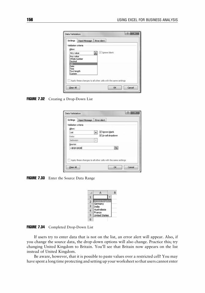
If users try to enter data that is not on the list, an error alert will appear. Also, ifyou change the source data, the drop-down options will also change. Practice this; trychanging United Kingdom to Britain. You’ll see that Britain now appears on the listinstead of United Kingdom.

Be aware, however, that it is possible to paste values over a restricted cell! You mayhave spent a long timeprotecting and setting up yourworksheet so that users cannot enter

FIGURE 7.34 Completed Drop-Down List

FIGURE 7.33 Enter the Source Data Range

FIGURE 7.32 Creating a Drop-Down List

c07 23 June 2012; 12:17:31


incorrect data; however, it is very easy for users to inadvertently (or perhaps deliberately)paste over a data validation without receiving the error message or restrictions thatwould have appeared had they tried to enter the data directly into the cell.

Referencing Source Data on Another Sheet

A restriction with data validation drop-downs is that the source data and the drop-down must be on the same page. There is a workaround, however.

1. Assign a named range to the source data (for example, 5countries). See the sectionon “NamedRanges” inChapter 5 for instructions on how to do this. See Figure 7.35.

2. When creating the data-validation drop-down, in the List box, enter an equal signfollowed by the name of the range on the other worksheet. You must type ¼ andthen spell the named range correctly for it to work.

Note that in Excel 2010, it is possible to link directly to source data on other sheetswhen creating a data-validation drop-down box without having to use a named range.However, if this is done in 2010 without using the named range, then the file will not becompatible with Excel 2007 or 2003. It is therefore recommended to always use namedranges when linking drop-down boxes to source data on another page to ensurecompatibility with earlier versions of Excel.

FORM CONTROLS

Form controls are objects such as drop-down boxes and option buttons that sit over thetop of Excel sheets, like charts do. They can interact with formulas so that when theoption is selected, it changes the formula and can drive the model. They can be espe-cially useful for scenario selection and assumptions in a financial model.

Building form controls into a financial model can be time-consuming for themodeller, but they do make the model look very professional and the interface becomesextremely easy to use.

FIGURE 7.35 Creating a Drop-Down List Using a Named Range

c07 23 June 2012; 12:17:31


Accessing Form Controls

If you are using Excel 2007 or 2010, you will need to have the Developer tab showingin the ribbon. If you cannot see it in the ribbon, you’ll need to change your options.

Showing the Developer Tab in the Ribbon

This section is only relevant for Excel 2007/2010 and Excel for Mac 2011 users. TheDeveloper tab contains several functions that are useful when developing macros andform controls. The default installation version of Excel 2007 or 2010 will not have theDeveloper tab showing in the ribbon. You will need to change this setting only once,unless you re-install Excel, or move to another machine.

This is one of the few instances where the instructions for 2010 differ from 2007.To display the Developer tab in the ribbon in Excel 2010:

1. Click on the File menu in the top left-hand corner of your screen.2. Scroll down to Options at the very bottom and select it.3. Select Customize Ribbon.4. In the box to your right, tick the Developer box.

In Excel 2007:

1. You need to click on the Microsoft Office button in the top left-hand corner ofyour screen.

2. Under Excel Options, go to the Popular section.3. Check the Show Developer Tab in the Ribbon.

And in Excel for Mac 2011:

1. Click on the gear box in the top left-hand corner of your screen.2. Select Ribbon Preferences.3. In the dialog, tick the Developer box.

You don’t need to do any of this if you are using Excel 2003, as it doesn’t have aDeveloper tab; macros and form controls are directly accessible via the toolbar in Excel2003. See Figure 7.36.

FIGURE 7.36 The Developer Tab

c07 23 June 2012; 12:17:31


Check Boxes

Tick boxes (or check boxes, as Microsoft calls them) are very handy tools that can helpusers choose their desired options from a list. By building check boxes into a financialmodel, the developer allows users to customise the model by adjusting the combina-tions of inputs for the financial model’s assumptions.

HOW TO CREATE CHECK BOXES

1. Go to the Developer tab on the Excel toolbar and click on Insert. See Figure7.37. If you cannot see the Developer tab, follow the instructions above onhow to show the Developer tab in the ribbon.

FIGURE 7.37 Insert Controls Icon

In Excel for Mac 2011: Below is how the Developer tab in the ribbonlooks if you are using Excel for Mac 2011. See Figure 7.38.

FIGURE 7.38 Form Controls in Excel for Mac

2. From the Forms Controls menu select the check box as shown in Figure 7.39.

FIGURE 7.39 Inserting the Check Box

(continued)

c07 23 June 2012; 12:17:32


(Continued)

3. Draw the check box, and you should see the box with a name Check Box 1.Subsequent check box names will be Check Box 2, Check Box 3, and so on.For ease of use and understanding, you must place the check box next to theitem in the list you want to check.

Note that you can change the check box name to anything you prefer. In thisexample, the itemname itself hasbeenused tokeep things simple. SeeFigure7.40.

FIGURE 7.40 Check Box in the Sheet

4. You can now link the tick mark in this box to any function in your financialmodel. To do that you need to open the Format Control associated with thecheck box. This can be done in two ways.

a. Right-clickon thecheckboxandselectFormatControl as showninFigure7.41.

FIGURE 7.41 Assigning Check Box Options

(continued)

c07 23 June 2012; 12:17:32


b. Alternatively, select the check box and click Properties on the ribbonunder the Developer tab, as shown in Figure 7.42.

FIGURE 7.42 Check Box Properties

5. In the Format Control dialog you can select the default value of the checkbox (unchecked, checked, or mixed) and the cell to which you want to linkthe check box status. In Figure 7.43, it is linked to C5. To enhance the look ofthe check box, you can select 3-D shading.

FIGURE 7.43 Format Control Dialog Box

6. The cell to which the status is linked will have a Boolean value of TRUE orFALSE. Seemore detail in “BooleanLogic (BinaryCodes)” later in this chapter.

(continued)

(Continued)

c07 23 June 2012; 12:17:33


Option Button

Sometimes users may need to choose one item from a list, which drives the rest of thecalculations and analyses. The Option button (sometimes called a Radio button) offersyou the ability to create this logic to restrict the number of options users can choose inthe financial model.

(Continued)

7. You can add multiple check boxes corresponding to the items in the list.Based on the Boolean status, you can design your financial model to pick therespective items. See Figure 7.44.

FIGURE 7.44 Worksheet Showing Check Boxes

8. Practice adding multiple items to the list and associating check boxes to eachitem.

HOW TO CREATE OPTION BUTTONS

1. Go to the Developer tab on the Excel toolbar and click Insert.

2. From the Forms Controls select the Option Button, as shown in Figure 7.45.

In Excel for Mac 2011, go to the Developer tab on the Excel toolbar.Select Radio Button, as shown in Figure 7.46.

3. Draw the Options button in front of the item in the list. Like the check boxes,the Option button default name starts with Option Button 1 and increaseswith each new button. The name can be later customised. See Figure 7.47.

4. You can edit the properties of the button using Format Control. You canaccess the format control dialog in the same manner as for check boxes.

(continued )

c07 23 June 2012; 12:17:33


FIGURE 7.45 Inserting the Option Button

FIGURE 7.46 Radio Button in Excel for Mac

FIGURE 7.47 Worksheet with Option Button

a. Right-click—Format Control.b. Click Properties in the ribbon under the Developer tab.

5. In the Format Control dialog box you can select the default value ofthe option button (unchecked or checked) and the cell to which you want tolink the option button status. (Here it is linked to D5.) To enhance the lookof the option button you can select 3D shading. See Figure 7.48.

(continued)

(Continued)

c07 23 June 2012; 12:17:33


1By design, all the Option buttons will always refer to a single cell, unlike check boxes. If youchange the cell link for one option button, it will automatically update the rest.


6. The cell to which the status is linked will have a numerical value of the itemin the list1. In the Figure 7.49, the fourth item was selected, hence $D$5 ¼ 4.

FIGURE 7.49 Worksheet with Option Button

7. You can add multiple option buttons corresponding to the items in the list.Based on the item number selected, you can design your financial model tocarry out the necessary analysis.

8. Practice adding multiple items to the list and associating option buttons toeach item. As you switch between each item in the list you can observe thenumber change in the linked cell.

(Continued)

c07 23 June 2012; 12:17:34


Spin Buttons

Spin buttons are useful for controlling what users can enter into the input fields in yourfinancial models. By including a spin button, users can increase or decrease the numberin the increments that you specify. For example, if you set it to increments of 5, and thecurrent value is 400, when user hit the up arrow, it will change to 405, then 410, 415,and so on, and the same with the down arrow.

HOW TO CREATE A SPIN BUTTON

1. Go to the Developer tab on the Excel toolbar and click on Insert.

2. From the Forms Controls select the Spin Button, as shown in Figure 7.50.

FIGURE 7.50 Inserting the Spinner

In Excel for Mac 2011, go to the Developer tab on the Excel toolbar.Select the Spin Button.

3. Draw the spin button next to the input box for the value you want to control.Figure 7.51 shows an example of the spin button.

FIGURE 7.51 Completed Spin Button

4. You can edit the properties of the button using Format Control. You canaccess the format-control dialog in the same manner as for a check box.


(continued)

c07 23 June 2012; 12:17:34


Combo Boxes

Creating a drop-down box is an important tool in many user-friendly models where themodeller wants the user to select from a pre-defined number of options, making themodel easier to use, and also avoiding mistyping and potential errors. The advantage ofthe combo boxes is that you eliminate any ambiguity in user inputs and still keep thingssimple for users to provide the inputs. See Figure 7.53.

The combo box is an alternative to using the data-validation drop-down tool. Seethe section on “Bulletproofing Your Model” earlier in this chapter for instructions on

5. In the Format Control dialog, you can specify the current or default value inthe cell, the minimum value (here it is set to 0), maximum value (here it is1,000), and the incremental change (here it is 10). You must also specify thecell in which you want to change the values in the cell link. See Figure 7.52.


6. Practice pressing the arrows up and down.

FIGURE 7.53 Completed Combo Box Drop-Down

(Continued)

c07 23 June 2012; 12:17:34


HOW TO CREATE A COMBO BOX

1. Go to the Developer tab on the Excel toolbar and click on Insert.

2. From the Forms Controls select the Combo Box as shown in Figure 7.54.

FIGURE 7.54 Inserting the Combo Box

In Excel for Mac 2011, note that combo boxes can only be used inconjunction with VBA in Excel for Mac 2011, and therefore the instructionsin this section do not apply to Mac users. Please see the “Macros” section inChapter 8 for more details on how to use VBA to build form controls in Excelfor Mac 2011.

3. Draw the combo box next to the input box for which you want to controlinput. Figure 7.55 shows an example of the combo box.

FIGURE 7.55 Drawing the Combo Box

(continued)

c07 23 June 2012; 12:17:35


4. To fix the inputs, create an input box with inputs such as shown in Figure7.56. Here we are using the range B8:C11.

FIGURE 7.56 Scenario Source Data

5. You can now associate these inputs with your combo box using FormatControl. You can access the Format Control dialog box in the same manneras for check box.


6. In the Format Control dialog, give the Input Range (here it is B9:B11), andthe Cell Link (here it is $D$8). Select 3-D shading to enhance the combo box.See Figure 7.57.


(continued)

(Continued)

c07 23 June 2012; 12:17:35


how to create a data-validation, in-cell drop-down box. The only advantage of thecombo box is that the drop-down arrow is visible whether the cell is selected or not.This is a significant advantage if users are not very Excel savvy.

From the modeller’s perspective, however, a combo box takes much longer tobuild, requiring more cells for the process, and is therefore less efficient. For thesereasons, most modellers prefer the data-validation drop-down tool.

Boolean Logic (Binary Code)

Most form controls use Boolean logic, which converts everything one of to two values:a one or a zero. For example, if a check box is ticked, it will return a value in the outputcell of TRUE, which equals 1; and if it is un-ticked, it will be FALSE, which equals zero.We can use the output cell to drive a formula.

This relation will only indicate the item number selected; so D8 wouldreflect 1 for optimistic, 2 for likely, and 3 for pessimistic. To translate thesenumbers into meaningful percentages from the chart, you need to link col-umn C to D8; this can be done using IF or INDEX functions in Excel.

7. INDEX is a more elegant way of representing this link. Use the formula¼INDEX(B9:C11,D8,2) to create the necessary linkage. See Figure 7.58.

FIGURE 7.58 Using the Combo Box Output in a Formula

8. To keep the form clean, typically modellers would change the font colour ofcell D8 to white so that the text is invisible to the user but available forcalculation.

9. Practice changing the combo box, and see the values change.

(Continued)

c07 23 June 2012; 12:17:36


In Figure 7.59, the output cell is B5. When the check box is ticked, it shows thevalue TRUE, which is equal to one, so this has been done by using the formula:

¼B7*((B5*B2)þ1)

If the check box is left un-ticked, the output cell would display FALSE, which givesthe value zero, and according to the formula, the GST would then not be included inthe total. See Figure 7.60.

Similar formulas can be created to link to other form controls such as optionbuttons and combo boxes.

Form Controls versus ActiveX Controls

If you are using Excel 2007 or 2010, you may have observed that the Insert buttonunder the Developer tab has two set of options: form control and activeX controls.While both have the same set of functions, they have a slight difference. The ActiveXcontrols are tailor-made for a Microsoft Office environment and use MicrosoftActiveX to enhance their functionality. If you are absolutely certain that your financial

FIGURE 7.59 Ticked Check Boxes Drive Calculation

FIGURE 7.60 Un-Ticked Check Boxes Drive Calculation

c07 23 June 2012; 12:17:36


model would be used in the MS Office environment only, then you could possibly add afew additional enhancements to your controls. However if your users might also beusing other environments like Mac OS, the ActiveX controls can cause problems—asApple’s operating system does not support Microsoft ActiveX.

If you want to keep your financial modelling product platform independent, stickto form controls. As far as core functionality is concerned, Form controls will offer youall the necessary flexibility required for a smooth user experience.

SUMMARY

Formatting and displaying the data and inputs are important parts of building afinancial model. Of course the accuracy of the model and its calculation are mostimportant, but having a model that looks good and is easy to use certainly adds to theintegrity and usability of the model. A model with which the model builder hasobviously taken care to use clear colour coding, borders, and correct formatting will betrusted more, and given more credibility by the user. Therefore, most good modellerswill spend a little time (not too much) during the model build to format colours,borders, and styles to make it look better.

c07 23 June 2012; 12:17:36


c07 23 June 2012; 12:17:36

CHAPTER 8Tools for Financial Modelling

In this chapter, we’ll look at the basic, commonly used tools of hiding and grouping.We’ll then cover some more advanced tools such as array formulas, goal seeking,

pivot tables, and macros. Whilst the best financial models are the simplest and easiestto understand (and therefore often don’t contain these complex tools) it’s importantthat the financial modeller has a grasp on how to use these tools if functionalityrequires.

HIDING SECTIONS OF A MODEL

Being able to hide sections of a model is a very handy tool, especially when tidying up amodel to conceal cells that are necessary for the model to work, but not necessary forthe user to see. You can hide rows or columns in the model, or you can hide an entiresheet. If you have information in a model you don’t want users to see (for example,unnecessary detail or a calculation that will only serve to distract from the model), youcan hide the section of the model that contains the data.

Columns and Rows

It is possible to hide a column or row of data to stop it printing out, or to stop otherpeople from viewing it.

HOW TO HIDE A COLUMN OR ROW

1. Select the column or row by clicking on the heading.

2. Right-click and select Hide.

The column or row will be hidden from view. But if you look at the columnor row headings you can see which column is missing.

c08 22 June 2012; 18:30:29

173

TIP

If you have hidden column A, or row 1, it can be tricky to unhide it. You’ll need to holddown the mouse and select across the row or column headings left or upward inorder to unhide the column or row. Now the knack is that you have to right-click withthe mouse in the highlighted row or column, as shown in Figure 8.1. If you clickelsewhere, it won’t work.

You can hide multiple columns or rows at the same time. Just select all the columnsor rows at the same time and follow the steps outlined above.

Sheets

Hiding sheets is also very useful. If you have information on a model you do not wantusers to see at all, (e.g., salary information on budget models) you can hide the sheetwith sensitive information, and then protect the workbook. The hidden sheets disap-pear from view, but links are retained as the sheet has not been deleted from theworkbook.

FIGURE 8.1 Unhiding Rows 1 and 2

c08 22 June 2012; 18:30:30


NOTE

Although we can easily hide multiple worksheets at a time by selecting several sheets using the Controlkey, only one sheet can be unhidden at a time!

HOW TO VIEW (UNHIDE) A COLUMN OR ROW

The difficulty of bringing back a hidden column or row is that you need to selectit first. As it is hidden, you cannot see the row or column to click on it. The trickis to select the headings either side of the hidden column or row. This will selectthe columns or row before and after, as well as the hidden column or row itself.

1. Click and drag across the headings to select those before and after the hiddencolumn or row.

2. Right-click and select Unhide, as shown in Figure 8.2.

FIGURE 8.2 Unhiding Rows

TO HIDE OR UNHIDE A SHEET

1. Select the sheet(s) you want to hide or unhide.

2. Right-click on the sheet tab and select Hide/Unhide. (See the Excel 2003instructions available at www.wiley.com/go/steinfairhurst.)

c08 22 June 2012; 18:30:30

Tools for Financial Modelling 175


TIP

A way to hide a sheet even more securely is to change the properties of the sheet in theVisual Basic code to Very Hidden. This method is not commonly known and willensure that only a user experienced with programming will be able to work out how tounhide your sheets.

1. To try this out, right-click on the tab name of your worksheet, and select ViewCode, as shown in Figure 8.3.

FIGURE 8.3 Viewing the Source Code

In Excel for Mac 2011, select Tools, then Macro, then Visual Basic Editor.

2. This will bring up your Visual Basic Editor. This should look fairly similar in allversions of Excel.

3. Click on the sheet that you want to hide in the top left, and change propertiesof that sheet in the bottom left from Visible to Very Hidden, as shown inFigure 8.4.

By default, all sheets are set to Visible. If you change the properties to Hidden, thiswill change the sheet so that it is hidden using the ordinary Hide Sheets tool, and it canbe unhidden as easily as normal. If it is “Very Hidden” it cannot be seen even when youtry to unhide the sheets. The only way to unhide a Very Hidden sheet is to change theproperties in the VBA code!

c08 22 June 2012; 18:30:31


Using Protection As just outlined, there are two methods of hiding: either hide rows andcolumns, or hide the worksheet itself. Depending on what is hidden, you might want touse another layer of protection to ensure that the data cannot be viewed. Passwordprotection is a good option in such a case.

See the section on “Bulletproofing Your Model” in Chapter 7 for more detail onhow to apply protection to models.

Errors Caused by Hiding

Hidden sheets, rows, and columns may hide complexity from the user and make themodel less confusing, but many users don’t like using what they perceive to be a blackbox. It’s up to you, the model developer, to decide how much power you will give tomodel users. If you hide everything and then protect the model so that they can’t seehow it has been calculated, this makes the model easy to use, but it does not inspireconfidence in users. It often depends on who is using the model. If a model is for other

For more information on the Visual Basic Editor using macros, see the section on“Macros in Financial Modelling Case Studies” later in this chapter.

FIGURE 8.4 Changing the Visibility Options in the Visual Basic Editor

c08 22 June 2012; 18:30:31


modellers to use, they probably won’t appreciate being locked out of certain sections ofthe model, as they’d like to check it for themselves to ensure that it is working properly.If users have limited Excel use, then hiding with protection is probably appropriate tomake sure they don’t mess up the formulas or make unauthorised changes.

There are many well-documented cases where hidden rows and columns have beenoverlooked in financial models and caused significant errors. In 2008, Barclays Capitalwas forced to file a legal relief motion relating to its acquisition of Lehman Brothers’U.S. assets after a reformatting error in an Excel spreadsheet resulted in 179 contractsbeing mistakenly included in the purchase agreement.

The spreadsheet contained nearly 1,000 rows with more than 24,000 individualcells and had to be reformatted and converted into a PDF document before beingposted on the bankruptcy court’s website by the end of the day.

But a junior associate reformatting the work was unaware that the original Exceldocument included hidden rows containing contracts that were marked with an n tosignify they should not be part of the deal.

The document was posted on the website, but the hidden cells had become visiblewhen the employee globally re-sized the rows in the spreadsheet—without the original ndesignations. The error was not spotted until Barclays posted a revised list of contracts,with notice to the affected parties.

For more Excel horror stories see the section on “Error Avoidance Strategies” inChapter 4. This story illustrates why it is highly recommended to use the GroupingTool when hiding rows and columns in financial models.

GROUPING

Determining whether there are hidden rows or columns on your worksheet can bedifficult. Using the grouping tool can make hidden data more obvious and avoid itsbeing overlooked.

HOW TO PROTECT HIDDEN SECTIONS OF A MODEL

If you have hidden rows or columns, apply the protection to the worksheet itselfby selecting Protect Sheet from the Review tab.

In Excel for Mac 2011, select Sheet from the Review tab in the Protectiongroup.

If you have hidden a sheet, apply protection to the structure of the workbook byselecting Protect WorkBook from the Review tab.

In Excel for Mac 2011, select Workbook from the Review tab in the Pro-tection group. (See the Excel 2003 instructions available at www.wiley.com/go/steinfairhurst.)

c08 22 June 2012; 18:30:31




Go to the Data tab and select Group/Ungroup from the Outline section. (See theExcel 2003 instructions available at www.wiley.com/go/steinfairhurst.) When group-ing is applied to a model, it will look like Figure 8.5 when collapsed.

It will look like Figure 8.6 when expanded.Notice the little 1 and 2 numbers in the top left-hand corner for the rows and the

columns. Clicking on these numbers is a very quick and easy way to expand and contracthidden rows and columns. Clicking 1 will contract the data, and 2 will expand it.

ARRAY FORMULAS

Array formulas are an advanced type of Excel calculation. Before we launch intowhat anarray formula is, let me begin by saying that I don’t recommend you include array

FIGURE 8.5 Collapsed Grouping

FIGURE 8.6 Expanded Grouping

c08 22 June 2012; 18:30:31



formulas in your models unless there is not possibly any other way. Array formulas canbe difficult to understand and hard to edit if you don’t know what they are, because youcannot change part of an array. In general, array formulas are very difficult to edit andaudit because they add a new layer of complexity that is often unnecessary. Most arrayformulas I have seen are usually built by consultants whowant to ensure that the client isunable to edit the model themselves, so guaranteeing themselves work in the future.

An array is basically just a collection of data of the same type that can be treated as asingle entity. An array formula treats the entire array as a single input to the formula. Thereason that array formulas are difficult to understand is because they don’t follow theusual rules of ordinary formulas. Trace Precedents and Trace Dependents will work onarrays, but don’t help very much! Many people don’t know how to use them, and if youhave never seen an array formula before, they can be pretty hard to work out. Therefore,if you are building a model for others to use, using array formulas is not a great ideabecause they need to make changes to the formula they may have trouble.

However, in order to seriously consider yourself an Excel super-user, you shouldknow how to build an array formula—or at least be able to recognise and edit one ifyou come across it—if only to remove it from the model, and replace it with a far moreauditable and user-friendly formula.

Array formulas are very powerful tools, and there are many reasons why analystsuse them. One of the main advantages is security—nobody can accidentally delete partof the array block when using an array formula. Also, because the data can bemanipulated as a whole block and used in the formula as a single unit, it’s a lot harderto make a mistake when building the formula.

You can identify an array formula because it includes curly brackets (like these: {}).Data tables are a type of array formula—probably one of the most useful ones—especially for the financial modeller. (See “Using Data Tables for Sensitivity Analysis”in Chapter 11 for how to build a data table.)

Advantages and Disadvantages of Using Array Formulas

The advantages of using array formulas are as follows:

n They ensure consistency because all formulas in the table are exactly the same.n A model containing arrays will use less memory and be more efficient.n Because it’s not possible to change a single cell on its own within an array formula,

it is unlikely that you or someone else will change your formula accidentally.n Because array formulas are difficult to understand, it means those with only basic

Excel knowledge are less likely to change (and mess up!) your formulas.n Array formulas do make it possible to perform some calculations that would oth-

erwise be impossible. This is really the only reason you should use an array formula!

The disadvantages of using array formulas are as follows:

n Although array formulas use less memory, if you use too many large arrays in onemodel it can slow down your calculation.

n You cannot use column references (such as A:A or D:D) in your array formulas.This is not best practice in financial modelling anyway, so no great loss!

n They are difficult to audit for many Excel users and require specialist skills, thoughthis can be considered both an advantage and a disadvantage.

c08 22 June 2012; 18:30:32


Simple Array Formula Example

1. Create two simple blocks of data (arrays) as shown in Figure 8.7.2. Highlight the block of cells C1:C5 and type/highlight 5A1:A5*B1:B5 in the

formula bar. See Figure 8.8.3. Now, hold down the Control and Shift keys while hitting Enter at the same time

(Control þ Shift þ Enter). Use the Command key first (Command þ Shift þEnter) in Excel for Mac 2011. See Figure 8.9.

FIGURE 8.7 Sample Data

FIGURE 8.8 Entering an Array Formula

FIGURE 8.9 Completed Array Formula

c08 22 June 2012; 18:30:32


4. The formula will appear in the whole array block. Note that curly brackets haveappeared around the formula.

5. Note that you now cannot make any changes to the array block.

Please also note that array formulas are sometimes referred to as CSE formulas,because you press Control þ Shift þ Enter to enter them.

Array Formula Uses

Financial modellers generally advocate the use of array formulas only when it is notpossible to do something any otherway. Some examples of these situations are as follows:

n Data tables are a form of array formula that is extremely useful for scenarios andsensitivity analysis in financial modelling. Instead of changing inputs one a time, anarray shows hypothetically what an outcome would be simultaneously in a singletable.

n TRANSPOSE allows you to transpose a range of data either vertically or hori-zontally, and retain links.

n Using a SUM and a VLOOKUP together as an array formula makes a very conciseformula. For example, 5SUM(VLOOKUP(value, list, {2,3,4},0)) will give you sumof values in rows 2, 3, and 4 instead of having to do 5VLOOKUP(value, list,2,0)1 VLOOKUP(value, list,3,0) 1 VLOOKUP(value, list,4,0). Note: You need tohold down Control, Shift, and Enter for this to work.

Transposing Data Using an Array

One of my favourite uses of an array formula is to create an ¼TRANSPOSE function,which will transpose data, allowing a link to be maintained within the model.

Let’s say you have the following data in a table. See Figure 8.10.And you’d like to transpose the data so that months and cities are switched around,

as shown in Figure 8.11.Before you start cutting and pasting, you could try the transpose values tool.

1. Highlight the original table, and copy it to the clipboard using Control þ C(Command þ C in Excel for Mac 2011).

2. Right-click in the cell that you want the data to appear, and select Paste Special.3. Tick the Transpose box as shown in Figure 8.12, and click OK.

This will paste all of the transposed values as hard-coded data in a new table. Usingthis method creates two separate, independent tables of data.

FIGURE 8.10 Temperature Data

c08 22 June 2012; 18:30:32


Using a TRANSPOSE Array Function However, you may wish to maintain the original tableas the source data, and have the second table linked to the first. Instead of linking eachcell individually (time-consuming and prone to error) you could use a TRANSPOSEArray Function.

1. Highlight a range with exactly the correct rows and columns for the destinationdata. (It’s probably easiest to use the Paste—Transpose procedures above todetermine exactly how big the range needs to be).

2. In the formula bar, type the formula 5TRANSPOSE (referencing the original data(i.e., 5TRANSPOSE(A2:M6)).

3. Now, hold down the Control and Shift keys while hitting Enter at the same time(Control þ Shift þ Enter) or Command þ Shift þ Enter in Excel for Mac 2011.

FIGURE 8.11 Transposed Temperature Data

FIGURE 8.12 Paste Special Dialog Box

c08 22 June 2012; 18:30:32


4. The formula will appear in the whole array block. Note that the curly brackets haveappeared around the formula, so the formula will be {=TRANSPOSE(A2:M6)}.

5. Note that changes you make in the original block of data will be reflected in thesecond block.

GOAL SEEKING

Goal seek is a very handy and commonly used tool in financial modelling and analysis.Goal seek is used to adjust the value in a specified cell until a formula dependent on thatcell reaches the result you specify. In other words, it will change the inputs such that theoutput is set to the exact amount you want it to be.

In order to run a goal seek, you must have:

n A formula.n A hard-coded cell that drives that formula.

The formula and its input cell do not need to be on the same sheet or even in thesame model. As long as there is a direct link between the two (no matter how manycalculations are in-between) the goal seek will work. However, it’s important toremember that the input cell must be hard-coded. An input cell that contains a formulawill not work.

A common use of goal seek is in break-even analysis. We normally want to knowhow many units we need to produce to break-even (i.e., how many units we need toproduce in order to recover our costs). In this instance, we’d change the number of unitsin the model until the profit amount is set to zero. See “Break-Even Analysis” inChapter 9 for an example of this.

Let’s say you borrow one million dollars at an interest rate of 6.5 percent.

1. Use the PMT function to calculate the monthly repayments over 15 years.2. If you use the PMT formula wizard, your input should look as shown in

Figure 8.13.3. The result will be -$8,711. Put a minus sign in front of it to make it a positive

number.4. Your formula should be 5-PMT(B2/12,B3*12,B1).

See “Loan Calculations” in Chapter 6 for more detail on how to use PMTand other loan calculation functions.

Let’s say that we can afford for our repayments to go up to, say, $10,000 permonth. How much of an increase in interest payments can we afford? Maybe weshould fix our rate.

5. On the Data tab, in the Data Tools group, click on What-if Analysis and selectGoal Seek from the drop-down list. In Excel for Mac 2011, go to the Data tab.Then, in the Analysis group, click on What-if Analysis and select Goal Seek fromthe drop-down list. (See the Excel 2003 instructions available at www.wiley.com/go/steinfairhurst.)

6. In the Set Cell box, enter the reference for the cell containing the formula thatproduces the desired end result (B4, in this case).

c08 22 June 2012; 18:30:33




7. In the To Value box, enter the result you would like to achieve in the Set Cell(type in 10000).

8. In the By Changing Cell, enter the reference for the cell that Excel is to change(B2, the interest rate).

9. This will bring up the Goal Seek Status dialog box containing the result of yourseek. See Figure 8.14.

10. Click OK to accept the new values, or Cancel to go back to the original values.

The answer to this problem is that we can afford for interest rates to increase to8.75 percent. If the bank were to offer us a fixed interest rate of 8 percent, then weshould take it!

FIGURE 8.13 Loan-Repayment Calculation Using PMT Function

FIGURE 8.14 Goal Seek Dialog Box

c08 22 June 2012; 18:30:33


While this calculation could have been done by trial and error, it’s much quicker touse a goal seek. Goal seek will work in huge models and run through a large number ofcalculations, giving the result you need to achieve your desired outcome.

PIVOT TABLES

Excel pivot tables are a very useful and powerful feature of Excel. They can be used tosummarise, analyse, explore, and present your data. A pivot table is a great reportingtool that sorts and sums independent of the original data layout in the sheet.

For example, you can take the sales data with columns like salesperson, region, andproduct-wise revenues, and use pivot tables to quickly find out how products areperforming in each region. Figure 8.15 is a snapshot of a pivot table that has been usedto summarise the spend by each customer.

For how to create a pivot table from scratch, see “How to Create a Pivot Table” inthis chapter.

The layout of pivot tables changed significantly in the upgrade from Excel 2003 to2007. Although the basic functionality remains the same (with the usual improvementsin 2007), the wizard layout has changed to a field list, so if you were an avid pivot-tableuser in Excel 2003, the new layout does take some getting used to.

Using Pivot Tables in Financial Modelling

Useful as they are, pivot tables are not used very widely in financial modelling. This isbecause they are static until refreshed, and this does not fit very well with the meth-odology of most financial models. As discussed in earlier sections, the whole point offinancial modelling is that you are able to change the inputs, and the outputs change!

FIGURE 8.15 Source Data and Pivot Table

c08 22 June 2012; 18:30:33


It’s far too easy for a user to change the inputs, and then forget to refresh the pivottable. This results in using incorrect outputs from the model.

It is for this reason that I recommend the use of an alternative live, dynamic for-mula, such as SUMIF or SUMIFS, in place of a pivot table when building a classicfinancial model that depends on inputs being changed. See “Aggregation Functions” inChapter 6 for how to use the SUMIF and SUMIFS functions.

Whilst it is possible to change the settings so that the pivot table will automaticallyrefresh whenever the file is opened, there is no guarantee that the user will open andclose the file before using the data, and it cannot be relied upon.

It’s not a bad idea to change the settings to automatically refresh in any case,however. You can do this by right-clicking on a pivot table, then go to Pivot TableOptions. See Figure 8.16. On the Data Tab, select Refresh data when opening the file.(See the Excel 2003 instructions available at www.wiley.com/go/steinfairhurst.)

Common Uses of Pivot Tables Pivot tables are more widely used in management reportingthan in pure financial models.

Here are some commonly used examples of pivot tables:

n Summarising data, such as finding the average sales for each region and for eachproduct, from a product sales data table.

n Listing unique values in any column of a table (this can also be done with theremove duplicates functionality of Excel 2007/10). Prior to the Excel 2007 release,pivot tables were a common way of obtaining a unique list.

n Filtering, sorting, and drilling down data in the reports without writing any for-mulas or macros.

n Transposing data (i.e., moving rows to columns or columns to rows).

FIGURE 8.16 Pivot Table Options Dialog Box

c08 22 June 2012; 18:30:34



Other Things You Should Know about Pivot Tables

n You can apply any formatting to the pivot tables. Excel has some very good pivottable formats (and they are better in the newer versions of Excel).

n You can easily change the pivot table summary formulas. Right-click on the pivottable and select the Summarise Data By option.

n You can also apply conditional formatting to pivot tables, although you may wantto be a bit careful as pivot tables scale in size depending on the data.

n Whenever the original data from which pivot tables are constructed changes, justright-click on the pivot table and select Refresh Data.

TIP

If youwant to drill downon a particular summary value, just double-click on it. Excelwillcreate a new sheet with the data corresponding to that pivot report value. It’s very useful!

How to Create a Pivot Table

When you need to create a report forecasting your fees by department and area, youcan follow these instructions:

1. Highlight the entire database, ensuring that the headings are at the top of the range.2. Select Pivot Table from the Insert tab, in the Tables section (found in the Data tab,

in the Analysis section in Excel for Mac 2011). See Figure 8.17.

FIGURE 8.17 Pivot Data Source Data

c08 22 June 2012; 18:30:34


3. The wizard will appear, and simply click OK.4. By default, it will put your pivot table on a new page. If you prefer, you can change

the options to locate it on the existing or a different page. The pivot table Field Listwill appear on the right-hand side.

FIGURE 8.18 Summarised Pivot Table

FIGURE 8.19 Completed Pivot Table with Field List in Excel 2010

c08 22 June 2012; 18:30:34


5. If you drag Customers into the Row Labels field and Price into the Values field, itwill summarise your data and create a pivot table report that looks likeFigure 8.18.

6. If you drag the Customers field to the Row Labels field below the Product field, itwill split your report into subcategories. See Figure 8.19.

Thepivot table cannowbequickly formattedusing thedrop-downstylesontheDesigntab. (See the Excel 2003 instructions available at www.wiley.com/go/steinfairhurst.)

MACROS

Many aspiring modellers think that they need to be proficient in macro-building inorder to become serious financial modellers. Whilst it’s not a bad idea to have aworking knowledge of macros—and the language they are built in, Visual Basic forApplications (VBA)—it’s certainly not critical for a financial modeller to become asuper VBA programmer. As discussed in previous sections, the best sort of financialmodel uses the simplest tools, and introducing macros to a financial model brings awhole new level of complexity.

Before launching further into the pros and cons of including macros in yourfinancial model, let’s have a quick overview of what macros are and how to buildthem. VBA in Excel is a huge topic in itself and one I’m not planning on going intotoo deeply here. Once you start writing macros it’s quite easy to get hooked, as youcan do some truly amazing things in Excel, which will bring the functionality of yourwork to a whole new level. If you develop an interest in the subject, there are lots ofbooks and training courses specifically on macros and VBA. Make sure that you buy abook or attend a course that is specifically on VBA for Excel and its use in finance, asthere is a lot of programming that is done in VBA that is not finance-related.

A macro is a collection of commands that are performed in a set order. A macroenables you to repeat operations that you would normally do by hand, but it is muchfaster and, when written correctly, much more reliable. Often, a macro will do inseconds what takes hours or days by hand. It can also perform tasks that are physicallyimpossible manually. If you find you are performing the same commands or actionsover and over again, in exactly the same sequence, you can create a macro to record allthose actions for you. You can then assign the macro to a button and run it using asingle click. You can even assign the macro to a keyboard command.

Macro Settings

Before we begin creating macros, there are a few settings in Excel you’ll need to change:

n Showing the Developer tab in the ribbon is not strictly required to record and runmacros, but it contains tools that makes it easier to run and edit macros, as well assome handy control tools and buttons.

n Changing the security settings is required, and you must change this setting if youwant to run macros.

c08 22 June 2012; 18:30:34



The default installation version of Excel does not have these settings. You will needto change these settings only once, and you will not need to do it again unless youre-install Excel, or move to another machine.

Showing the Developer Tab in the Ribbon This is only relevant for Excel 2007/10 and Excelfor Mac 2011 users. While it is possible to record a macro by clicking on the launchbutton in the bottom left-hand corner of your screen, as shown in Figure 8.20, theDeveloper tab contains other functions that are useful when developing macros andother tools, so it’s best to install the Developer tab.

If you do not see the Developer tab, click on File—Options—Customize Ribbon.Check the Developer box. Excel for Mac 2011 users go to Excel—Excel Preferences—Ribbon and check the Developer box. For more detailed instructions on how to dothis, read “Showing the Developer Tab in the Ribbon,” under “Form Controls” inChapter 7.

Setting Macro Security Levels Macros perform various automated functions that run viaexecutable code. While most macros are useful and harmless, some malicious macroviruses can destroy data or otherwise damage your machine. For this reason, manypeople decide to disable macros altogether or turn security up so that macros canonly be run from documents written by trusted publishers. However, turning up thesecurity may disable legitimate macros, so changing the security level is a personaldecision. You may also want to change this setting before you open documents fromdifferent sources.

You will need to decide on the level of security appropriate for the way that youwork. If you only ever run macros that you have written yourself, then Low may besuitable. High will be difficult to work with, as it won’t allow you to run macros at all.If you are often running macros from a trusted location, you may choose to select theEnable All Macros option.

FIGURE 8.20 Macro Launch Button

c08 22 June 2012; 18:30:35


To change your macro security settings:

1. Click on the File menu or the Microsoft Office Button in the top left-hand cornerof your screen.

2. Scroll down to Options or Excel Options at the very bottom and select it.3. Select Trust Center and click on Trust Center Settings.4. Choose the desired level of security.5. Close the model down, and then reopen it.

In Excel for Mac 2011:

1. Click on the Excel menu at top left-hand corner of your screen.2. Click Preferences.3. Click the Security button, and go to the Macro Security section.4. Choose the desired level of security.5. Close the model down, and then reopen it.

For Excel 2003, see the instructions available at www.wiley.com/go/steinfairhurst.

Recording and Running a Simple Macro

The best way to get started with macros is to record one.

TO RECORD A MACRO

These are the basic steps to create a simple macro by recording it. In the View tab intheMacros section, click on the arrowunder theMacrobutton, thenRecordMacro.(See the Excel 2003 instructions available at www.wiley.com/go/steinfairhurst.)

In Excel for Mac 2011, click the Record button in the Developer ribbon inthe Visual Basic section.

See Figure 8.21.

FIGURE 8.21 Record Macro Dialog Box(continued)

c08 22 June 2012; 18:30:35




This macro will save within the Excel you used when recording the macro. Thismacro is available whenever you have the file open.

Practical Exercise Let’s try recording a macro that will be useful. Say you want tochange the formatting of a cell from 150000 to $150,000—a very commonly per-formed task. (This macro will be useful, as it’s not possible change this formatting witha single mouse click or keystroke.) Follow these instructions:

1. Type 150000 into cell A1 on a blank worksheet.2. Begin recording, as shown above. Call the macro FormatCurrency. Assign a

shortcut key (e.g., Ctrl þ m), and click OK. See Figure 8.22.3. Select cell A1, and change the formatting to $150,000. This can be done through

the menu bar, or right-click, Format cells, and change the currency to the desiredformat.

Excel will come up with the suggested name Macro1. You can type over this.Macro names must be one word with no spaces. It is best to give the macro aname that relates to what it does (i.e., PrintCompanyData), rather than a non-descriptive name such as Macro1. Type a name for the macro into the MacroName box. You can also allocate a shortcut key.

You are now recording your macro. Every command or action you performwill be added to the macro.

1. Performall the actions youwish to be included in themacro. For example, print,save, change colour, and insert or delete rows and columns, will all be includedin the macro if you perform these actions while the macro is recording.

2. When you wish to stop recording the macro, click on the arrow under theMacro button, then Stop Recording. In Excel for Mac 2011, in the Developerribbon in the Visual Basic section, click the Record button again, which willstop the recording.

TO RUN THE MACRO

1. In the View tab in the Macros section, click the Macro button.

In Excel for Mac 2011, click the Macro in the Developer ribbon inthe Visual Basic section.

This will bring up the Macro dialog box, containing a list of all theavailable macros.

2. Click in the list to select the macro you wish to run.

3. Click on the Run button. All the actions you performed in the steps abovewill repeat themselves.

(Continued)

c08 22 June 2012; 18:30:35


4. Stop recording.5. Now we can test to see if the macro worked. Go back to cell A1 and change the

formatting to a percentage, for example.6. Then run the macro as shown above. The formatting of cell A1 will revert to the

formatting we specified in the macro. Now we can edit the macro and makechanges within the VBA code as follows:a. Select the Macros icon from the View or Developer tab on the ribbon (the

Visual Basic tab in Excel for Mac 2011). The Macro dialog box contains a listof all the available macros.

b. Select the macro that you want to edit, and press Edit. This will take you into theVisualBasic forApplications coding editor,whereyou canmanually edit amacro.

c. Change things such as sheet names or cell references, rather than re-recordingthe macro. You can even make the macro run more efficiently by removing theduplication of the .select command.

d. Change the code, and close down the editor.7. Now we can edit our macro. Go into the VBA editor, as shown above. If you

haven’t been into the editor before, it can seem a bit scary, but don’t worry. Youcan always close down the editor to get back into your Excel model.

8. The screen should look something like Figure 8.23.The text in green font is purely descriptive text. Any text preceded by the

apostrophe (’) will be ignored by the macro when running. You can delete orreplace this with documentation of your own, describing what the macro does.

FIGURE 8.22 Naming the Recorded Macro

FIGURE 8.23 Viewing the Recorded Macro in the VBA Editor

c08 22 June 2012; 18:30:36


Take a look at the code. It contains two steps: It selects cell A1, and formatsit as we have specified. This means that every time we run this macro, it willselect cell A1 and format it. If we remove the reference to cell A1, it will changethe formatting of whatever cell is selected. This is much more useful!

9. Remove the descriptive text and the first line of code. Your code should now say:

Sub FormatCurrency()Selection.NumberFormat 5 "$#,##0"End Sub

10. Close down the VBA editor and return to your model.11. Type some random numbers anywhere in your model—even on a different page.12. Select the cells, and run the macro. These numbers should change to your desired

format.

Creating Macro Buttons

You can assign a macro to almost any object or shape on your Excel worksheet,including shapes, buttons, and even combo-box drop-downs. The most commonly usedobject is a rectangular-shaped button. There are two ways of creating these buttons,either as shapes or traditional form buttons.

Macros in Financial Modelling Case Studies

There are hundreds of situations where macros can save time and increase accuracy.They might not necessarily be built and saved within financial models, but they could

HOW TO CREATE A SHAPE

1. On the Insert tab, in the Illustrations group, a Drawing Shape can be used asa macro button. Use Autoshapes (Insert—Shape ... in Excel for Mac 2011).The style can be changed to look like a purple rectangular button. (See theExcel 2003 instructions available at www.wiley.com/go/steinfairhurst.)

2. Right-click to add text that says press me.

3. Right-click to assign the macro to the button. Whenever you press thisbutton, the assigned macro will automatically run.

Alternatively, the more traditional macro button can be used.If you wish to create a traditional form macro button in Excel 2007/10,

it’s still possible, but it’s been hidden very well. You need to have theDeveloper tab showing before you can create these buttons. See the explana-tion from earlier in this chapter on how to make the Developer tab show inthe ribbon.

c08 22 June 2012; 18:30:36



HOW TO CREATE A TRADITIONAL FORM BUTTON

1. On the Developer tab, in the Controls group, select the Insert button andselect the Form button, as shown in Figure 8.24.

FIGURE 8.24 Inserting the Button in Excel 2007/10

On the Developer tab, in the Form Controls group, select the Buttonbutton. See Figures 8.25 and 8.26. (See the Excel 2003 instructions availableat www.wiley.com/go/steinfairhurst.)

FIGURE 8.25 Form Controls Ribbon in Excel for Mac 2011

FIGURE 8.26 Forms Toolbar in Excel 2003

(continued)

c08 22 June 2012; 18:30:36



be used in the collection of the data that goes into model. Here is a small sample of afew of the most common problems in financial modelling that are solved by macros.

n A company is doing a salary comparison between different countries, and wants toknow how much they would need to pay in Malaysian ringgit so that their salary isthe same as someone working in Singapore. If a worker in Malaysia earns theequivalent of 100,000 MYR after tax, how much would the company need to paythe worker before tax? The problem is that tax is calculated on pre-tax salary, soour formula gives us a circular reference. We can use a macro with a goal seek torepeatedly set the pre-tax salary to the amount entered by the user.

n Fifty identical budget templates have been created, and you discover a formulaneeds to be changed. Instead of making the change 50 times, record a macro. It willbe much quicker, and far less prone to error.

n A non-profit organisation sets its pricing so that all costs are fully recovered to breakeven. The costs keep changing, though, and the user is a senior account manager whodoesn’t know how to do a goal seek in Excel. The modeller creates a simple macrousing a goal seek so that all the user needs todo is change the costs andpress the buttonto find out how much the pricing needs to change to under the new costing.

n A dump of information containing several thousand rows is exported from adatabase into Excel every day. The data needs to be formatted and manipulatedmanually to be used in a daily takings report. Automating this with a macro canliterally save hours of manual data manipulation.

n A reporting model is built using a pivot table, but when new data is entered, theuser sometimes forgets to refresh the pivot table. The modeller builds a button torefresh a pivot table every time it’s pressed.

Dangers and Pitfalls of Using Macros

Wonderful as they are, macros should always be used with caution. Quite often for-mulas or filtering will achieve the desired result, without the need for building a macro.Always try a formula or standard Excel solution before considering the inclusion of amacro in your model.

n Unless ranges are defined properly using relative cell references, macros don’t movetheir references the way that formulas do. If any data has moved since the macro

(Continued )

2. Now click and drag over the spreadsheet to create the shape.

3. When you let go of the mouse button, the Assign Macro dialog box willappear. Select appropriate macro.

4. To change the assigned macro, right-click on the shape and click on AssignMacro.

5. You should add the appropriate text and format the shape with colour,shadow, and so on.

c08 22 June 2012; 18:30:37


was written, the macro will refer to the wrong cell. A badly written macro can copyand paste over data, and you won’t know what it has done!

n Visual Basic is a complex programming language, and a skill that many peopledon’t have. Therefore, many people are not able to edit or follow what a macro isdoing—especially if it hasn’t been documented properly.

n Macros are time-consuming to write, and often a much quicker and more trans-parent solution can be built just as easily with a plain formula.

n Running macros requires security settings to be changed (as shown above), and ifyour model is used by other people, they may not realise they need to change theirsettings, causing the model to not work properly.

n In Excel 2007/10 and Excel for Mac 2011, macro-enabled files need to be saved in.xlsm file format. If they are accidentally saved as an .xlsxmacro-free workbook, themacros will be removed from the file. If this happens, the macros have been deleted,and you’ll need to either rewrite the code, or copy it back in from a backup copy!

n Unless you will be maintaining the model yourself, most business Excel users havemore than enough to do without also trying to learn how to program.

n If you’re the one running the macro each time the model needs to be updated, that’sfine, but what will happen after you’re gone? If the process stops working due to amacro problem, it can hold up monthly procedures significantly.

Basically, there are more things that can go wrong if a financial model containsmacros. When it comes to building financial models, consider whether a VBA solutionis absolutely necessary before including it in your model. Macros should not be usedunless there is no other option!

USER-DEFINED FUNCTIONS (UDFS)

There may be times when expert modellers are restricted by the range of internalfunctions that Excel has to offer. To overcome these limitations, Excel offers what isknown as user-defined functions (UDFs). These are VBA-based mini functions that canbe created by users to suit their needs.

Note that user-defined functions are specialised uses for Visual Basic, and are notcommonly known to many users—even advanced financial modellers. If you decide tocreate user-defined functions, don’t expect that userswill be able to understandor edit them.

Benefits of UDFs

We don’t recommend the use of UDFs in financial models. However, if you do decide touse them, there are a number of benefits. Complex formulas can be reduced to a simplefunction,whichmakes it easier tobuild the financialmodel (butmoredifficult for someoneunfamiliar with UDFs to follow your calculations). UDFs also support array functions toevaluate a series of cells and give the flexibility of custom-designed text manipulation.

Drawbacks of UDFs

As with array formulas, the main drawback is that very few modellers will be able tounderstand or edit them. UDFs are not macros; hence they cannot be recorded, sotherefore you need good understanding of VBA to create them. Note also that, asformulas, UDFs cannot change the cell formats the way that macros can.

c08 22 June 2012; 18:30:37


UDFs can also be included as add-ins, but having such add-ins makes it difficult toshare the file with others. Add-ins mean one cannot decipher the function to trouble-shoot any glitches in the model logic.

Reusability: UDFs as Add-Ins

UDFs created in a spreadsheet can be reused in other sheets as add-ins. To save a spread-sheet as an add-in, select File, then Save As. Select Save As Type Excel Add-In (*.xlam).

When you want to use the add-in in another spreadsheet, simply import the add-in.

HOW TO IMPORT A UDF AS AN ADD-IN

1. Click on the Add-Ins button in the Add-Ins ribbon under Developer tab. SeeFigure 8.27.

FIGURE 8.27 Accessing the Add-Ins from the Ribbon

2. In the Add-Ins dialog box, click Browse to look up the UDF. See Figure 8.28.

FIGURE 8.28 Add-Ins Dialog Box

(continued)

c08 22 June 2012; 18:30:37


SUMMARY

The tools for financial modelling covered in this chapter range from the basic, such ashiding and grouping, to the more complex tools such as UDFs and array formulas. Asalways, we try to make our models as simple as possible, and as complex as necessary.Therefore, if you can create a model using just basic functions and tools, by all means,do so.

If, however, you find that your simple solution does not provide your model withthe desired functionality, then you may consider including a more complex nestedformula, or even possibly a macro. The best sort of financial models are those that areclearly laid out and use very simple and clearly defined tools—not because we don’tknow how to create complex models, but because they are easier to follow. So, inconclusion, it’s very difficult to be a top-notch financial modeller without knowing allthe complex tools and functionality in Excel, but that does not mean that you shoulduse these tools in every model. On the contrary, complex tools should only be usedwhen absolutely necessary.

(Continued )

3. If you have created a UDF add-in, you’ll see it listed here. Select the new add-in from the location and click OK.

4. The new add-in gets added to the list of add-ins in the dialog box. Select thenew add-in and click OK.

5. You can now use this function in the new spreadsheet just like the one inwhich it was created originally.

(See the Excel 2003 instructions available at www.wiley.com/go/steinfairhurst.)

c08 22 June 2012; 18:30:37




CHAPTER 9Common Uses of Toolsin Financial Modelling

Now that we know how to use many of the useful tools, functions, and features ofExcel, let’s take a look at actually using these tools to solve common problems,

calculations, and situations encountered in financial models.

ESCALATION METHODS FOR MODELLING

There are several different ways of applying a growth, indexation, or escalation methodover a period of time to a principal amount. We often need to be able to includeescalation in our models for the purpose of forecasting sales growth year over year forexample, or increasing costs by an inflation amount. Calculating a growth amountmight seem straightforward initially, but there are several different methods that can beused, and when applying growth rates in a model and you need to be clear about whichmethod you are using.

Whilst we can use functions to calculate future values based on set or varyinggrowth rates, we’ll firstly calculate them manually so that we understand the mechanicsof the calculations, and then use the functions.

Using Absolute (Fixed) Growth Rate

Herewe have compound growth over five years at a fixed interest rate. The capital growseach year by 5 percent. At the simplest level, our formula is base amount*(11growth).The reason we are adding 1 (effectively 100 percent) to the growth rate (5 percent) isbecausewewant the capital sum returned alongwith the accrued interest.Multiplying anamount by (1þgrowth) is a very common calculation in financial modelling.

Exercise: Fixed and Compounding

1. Create the exercise, as shown in Figure 9.1. The rate is fixed in a single cell (B4).Therefore we need an absolute reference, namely $B$4. So, after the first year (in2015) create the formula in cell C7: 5B7*(11$B$4).

2. Copy the formula in C7 to cells in D7 through G7.This method grows the amount at a fixed rate, which compounds each year.With most models we normally want to show the amount that is forecast in

each year, but if you want a shortcut formula that will show, in a single cell, how

c09 22 June 2012; 18:35:14

201

much we’ll have at a fixed, 5-percent growth after five years, we can use the FutureValue (FV) function. Let’s verify the amount you calculated for the year 2019 byusing this function.

3. Somewhere in a cell to the right of this table, enter Excel’s FV function. Either type5FV( into the cell and follow the prompts, or select FV from the function wizard.Because there are no periodic payments being made, we need to include the yearlyrate, the period in years, and the present value (PV).

4. Prefix the function with a minus symbol to get a positive result. Your formulashould be 5-FV($B$4,5,0,B7), and the totals using both methods should be thesame. Your sheet should look something like Figure 9.2.

Exercise: Fixed and Non-Compounding Another variation on this escalation method is tostill use a fixed growth rate, but not compound it. To do this, we will use an escalationindex across the top. This may be more practical in some model designs, but bear inmind that it yields different results. See Figure 9.3.

FIGURE 9.1 Fixed, Compounding Exercise

FIGURE 9.2 Completed Fixed, Compounding Exercise

FIGURE 9.3 Fixed, Non-Compounding Exercise

c09 22 June 2012; 18:35:15


1. In row 10, create your escalation index row using the formula 5B101$B$11 incell C9, and copying across.

2. Escalate in cell C14 by using the formula 5$B$14*C10, and copying across.

This formula gives you a lower result in Year 5 than the exercise examining fixedand compounding interest because it is not compounding on the previous year. Itsimply adds a flat $5,015 3 5 percent each year, instead of adding the growth rate tothe increased total.

Using Relative (Varying) Growth Rates

The next example returns the future value of an initial principal after applying a seriesof interest rates. While the rate was fixed in the example above, here it fluctuates fromyear to year. This is considered to be a superior model design, as it allows for fluctu-ation of growth rates. Even if the growth rate does not change from year to year, bybuilding the model in this way, we are allowing for changes in the future. By using theaforementioned design with a single growth rate, we are restricted to having only a ratethat does not change. See Figure 9.4.

We’ll no longer use absolute references for the interest rate, but will allow both itand the value to change from year to year as we copy the formula across D22 throughto G22. Cell C22’s formula is base amount*(11growth), as previously, but this timethe growth does not have an absolute reference applied to it. 5B22*(11B19).

Exercise: Relative and Compounding

1. Complete cell C22 in the exercise workbook to achieve the result above, then copythe result to the right.

Let’s try a shortcut function to get directly to the results without going throughthe annual calculations.

To the right of the results, enter Excel’s FVSCHEDULE function to verify thefigure for 2019.

Use the function FVSCHEDULE in your exercise spreadsheet. Note that theFVSCHEDULE function was new to Excel 2007 and therefore is not available inprevious versions of Excel.

Your sheet should look something like Figure 9.5.

Exercise: Relative and Non-Compounding In this next example, we are using anotherescalation index across the top. See Figure 9.6.

FIGURE 9.4 Relative, Compounding Exercise

c09 22 June 2012; 18:35:16

Common Uses of Tools in Financial Modelling 203

1. In row 25, create your escalation index row using the formula 5B251B26 in cellC25, and copying across.

2. Escalate in cell C29 by using the formula 5$B$29*C25, and copying across.

This formula gives you a lower result in Year 5 than of the fixed andcompounding example because it is not compounding on the previous year.

Using Exponential Operations on an Absolute (Fixed) Growth Rate

This exercise is similar to the first one, except that we will include the use of the caretsymbol (^) to perform exponential (to the power of) operations. For instance, 3 3 3 33¼ 27. So does 33 and, in Excel’s equivalent, 3^3.

Exercise: Complex Escalation Figure 9.7 shows compound growth over a period at afixed 5-percent per annum interest rate.

Our formula will allow for start and end dates to the period, in the form of:

Base amount*((100%1growth)^(End year-Start year))

FIGURE 9.6 Relative, Non-Compounding Exercise

FIGURE 9.5 Completed Relative, Compounding Exercise

FIGURE 9.7 Complex Escalation

c09 22 June 2012; 18:35:16


Excel will perform the exponential operation before the multiplication, so theencompassing set of brackets (greyed) is not essential. The formula in C37 is therefore

5$B$37*((11$B$4)^(C36-$B$36))

Note that instead of using End year-Start year, you may also insert a helper row atthe top to link to instead, which makes a slightly less complex formula. The nextexercise shows how this can be used.

1. Complete the formula for cell C22 and copy it across D37 through G37 to achievethe results in the diagram above.

2. The function 5-FV($B$34,G21-$B$36,0,B37) will verify the answer for the year2019.

Practical Usage of Exponential Growth Rates

You will notice that we achieve the same result ($6,401) under the fixed, compoundingexercise as we did under the relative and compounding exercise, but with a far lesscomplex formula. Using exponential growth rates is useful when you need to com-pound the growth rate, but want each cell to operate independently.

If, for example, you have start dates and end dates that need to be included in aformula as well as compounding escalation, you will need to use exponential growthrates. In Figure 9.8, we will create a formula to evaluate the start date and end date,only inserting the cost in the relevant years and then compounding the inflation.

This will require the IF and AND functions to be used in combination to establishwhether the column heading year falls within an employee’s start and end dates.

For instance, in English terms we will be checking that IF(AND(2013 .5Employee Startdate,2013 ,5 Employee EndDate) is true before writing inflation-escalated costs into the appropriate cell of column F. Otherwise we will write a zero.

Use the term in years (row 5) to exponentially escalate the costs (in column C). Forinstance, if the year 2013 (F6) meets the IF test, F7 will equate to Cost*(11inflation)^0,which leaves it, in this case, unchanged.

Your formula should be: 5IF(AND(F$6,5$E7,F$6.5$D7),$C7*(11inflation)^F$5,0)

And the sheet should look something like Figure 9.9.

FIGURE 9.8 Staff Calculation Using Exponential Growth Rates

c09 22 June 2012; 18:35:16


UNDERSTANDING NOMINAL AND EFFECTIVE (REAL) RATES

From a financial modelling perspective, there are two interesting aspects of nominaland effective rates that we should be aware of.

1. Escalation Calculations. We need to consider whether an escalation, growth rate,or indexation amount includes the effect of inflation (i.e., whether it is real oreffective) and what this actually means in real terms.

2. Loan Calculations. When comparing and calculating interest rates, the frequencyof compounding can make a difference to the amount of interest actually paid.This can be calculated in Excel using the EFFECT and NOMINAL functions.

When including escalation or growth rates into a financial model, we sometimesneed to consider whether the growth percentage is expressed as a nominal or real rate.Normally we express the growth percentage as a nominal rate, meaning that we don’ttake into consideration the effect of inflation or other factors that would impact thevalue of that rate. The real or effective rate will include the effect of other factors, suchas inflation, to give you the real or adjusted value.

For example, if you earn a $100,000 salary, and after a year of working for thecompany, your boss unexpectedly gives you a raise of 10 percent, you think you’regoing to have an extra $10,000 in your pocket, right? Well, not exactly. Theoretically,in the 12 months since you began working for the company, your cost of living hasincreased and eroded the purchasing power of your salary. Therefore, if we assume thatthe consumer price index (CPI), or rate of inflation, is 3 percent, then your $100,000 isnot buying you as much now as it did when you first started the job. To calculate theeffective salary increase that you received, you’d need to deduct the inflation fromthe raise. Your nominal increase was 10 percent, but the real or effective raise was only7 percent.

Normally when modelling escalation amounts, we use the nominal rate, and weknow, when considering the calculations, that it does not take into account the pur-chasing power in the future. For example, in the exercise described in the previouschapter, we indexed the sales revenue at 5 percent, as shown below. It goes withoutsaying that the 5 percent is a nominal amount. We know that the $6,401 that isreceived in Year 5 is not really $6,401 in today’s terms because inflation will haveeroded its purchasing power. See Figure 9.10.

FIGURE 9.9 Completed Staff Calculations

c09 22 June 2012; 18:35:17


Ifwewanted to compare an investment in today’s terms,we’d need to use the effectiverate, and to calculate this, we would simply deduct the inflation amount—let’s say it’s3 percent—from the growth rate, and hence our effective growth rate is 2 percent. Asalways, we need to be very explicit about the rates we have used. Note that expressingamounts in effective terms is not commonly used in financial models and unless otherwisestated the user would assume that a rate is nominal. Therefore, if you choose to use aneffective rate,make sure that you state it clearly as an assumption, as shown inFigure 9.11.

Adjusting Loan Rates with NOMINAL and EFFECT Functions

Calculating effective growth rates as outlined above is quite simple, and we certainlydon’t need a dedicated Excel function to calculate them. There is another use for thenominal and effective concept in finance, and the calculation is far more complex.Nominal and real rates affect mortgage calculations, too. As discussed in “Loan Cal-culations” in Chapter 6, due to the effect of compounding, we actually pay a higherinterest rate than is actually expressed in the nominal rate when quoted by the lender.Most loans are calculated and compounded daily, and therefore every single day wepay interest on the interest that was charged on the previous day.

The nominal rate is basically the simple interest rate for the complete period of themortgage (i.e., the rate you are quoted when you take out the loan). The effective ratetakes into account the compounding and will therefore be higher, depending on howfrequently the loan is compounded.

The nominal and effective rates in Excel are related as follows:

Effective interest rate ¼ 1þNominal interest rate

N

� �N

� 1

FIGURE 9.10 Escalation Formula

FIGURE 9.11 Assumption Documentation in Growth Calculations

c09 22 June 2012; 18:35:17


where N is equal to the number of compounding intervals in the year.As usual, Excel has made these calculations simple for us by offering two important

pre-defined functions to convert nominal to effective rates, and effective to nominal.These are NOMINAL and EFFECT. Note that the NOMINAL and EFFECT functionsare new to Excel 2007 and therefore are not available in previous versions of Excel.

NOMINAL() This function returns the annual nominal interest based on the effective rateand compounding intervals in the year. The syntax for this command is:

n NOMINAL (Effective_Rate, Compounding_Period), wheren Effective_Rate: The effective interest rate for the year.n Compounding_Period: The total number of compounding intervals in the year.

¼EFFECT() This function returns the effective interest based on the annual nominal rateand compounding intervals in the year. The syntax for this command is:

n EFFECT(Nominal_Rate, Compounding_Period), wheren Nominal_Rate: The annual nominal interest rate for the year.n Compounding_Period: The total number of compounding intervals in the year.

The screenshot in Figure 9.12 shows how the effective rate can be calculated fromnominal rate.

Exercise: Comparing Two Nominal and Effective Interest Rate Offers

Let’s say you need to borrow some money, and you’re offered two different interestrates from competing lenders

1. Lender A is offering a nominal rate of 7.9 percent, compounded daily.2. Lender B is advertising an effective rate of 8.2 percent, compounded monthly.

Which is the best deal? Here is how to arrive at the answer:

1. Set up the inputs side by side, so that you can compare the effective rates. SeeFigure 9.12.

2. Calculate the effective rate of Offer A using the EFFECT function.3. Your formula in cell B4 should be 5EFFECT(B2,B3).

The effective rate of Offer A is 8.2219 percent, which means that Offer B is infact a lower effective rate.

FIGURE 9.12 Comparison of Interest Rates Exercise

c09 22 June 2012; 18:35:17


Let’s calculate the nominal rate of Offer B, for interest’s sake.

4. Your formula in cell C2 should be 5NOMINAL(C4,C3).5. The sheet should look something like Figure 9.13.

Let’s see what effect the number of compounding periods has on the rate. If LenderA had compounded monthly instead of daily, would that have made a difference to theeffective rate? It certainly would! Change the number of periods in cell B3 from 365 to12, and we will see that this drops the effective rate to just slightly lower than that ofOffer B. See Figure 9.14.

Although only a very simple calculation this is a good example of how, by fol-lowing financial modelling best practice and linking the formulas to the hard-codedinput variables, we can easily perform sensitivity analysis on our numbers by changingthe calculation assumptions.

CALCULATING CUMULATIVE TOTALS

As always, we try to follow best practice when building financial models, and one ofthe important points of best practice is to ensure that formulas are as consistent aspossible. Calculating cumulative totals is a common calculation in financial modelling,and this is one such situation where ensuring consistent formulas can be tricky.

We need to calculate the cumulative number of customers in order to calculate therevenue, and Figure 9.15 shows one solution to the problem. It will achieve a correcttotal, but it necessitates using different formulas in adjacent cells.

FIGURE 9.13 Completed Comparison of Interest Rates Exercise

FIGURE 9.14 Comparison of Rates with Changed Compounding Periods

FIGURE 9.15 Cumulative Totals Using Inconsistent Formulas

c09 22 June 2012; 18:35:17


Sometimes this is the only solution (without creating an overly complicatedformula) and, if necessary, you may simply need to resign yourself to the fact thatconsistent formulas are not possible. There is, however, a simple solution: Using theformula 5SUM($B$3:B3) will achieve the same result with consistent formulas, asshown in Figure 9.16.

HOW TO CALCULATE A PAYBACK PERIOD

There is no suitable formula in Excel for calculating a payback period. However, thereare a couple of different ways of doing it. Demonstrated below are two methods, butthis is by no means an exhaustive list. The first method is very simple, but not veryaccurate, and the second is quite long-winded, but more precise.

Simple Payback Calculation

In a business case summary as shown inFigures 9.17 and9.18,we can see that the paybackperiod (the point atwhich the sumofour cash flowsbecomespositive) is between three andfour years—at 2016. We can easily estimate this by highlighting the cash totals for eachyear and looking at the sumamount at the bottomright-handcorner of the page.However,we would like to create a cell that automatically calculates the payback year so that asinputs change due to scenario and sensitivity analysis, the payback year will always beshown in the model, based on the cash flow amounts.

FIGURE 9.16 Cumulative Totals Using Consistent Formula

FIGURE 9.17 Manually Calculating the Payback Year

c09 22 June 2012; 18:35:18


1. Above the years, in cell B2, create a formula that calculates the cumulative amountof cash. See “Calculating Cumulative Totals” later in this chapter for how to dothis. Your formula should be 5SUM($B$13:B13).

2. In cell B15, insert a formula that will return the year in which the cumulativecash amount becomes positive. Your formula should be something like this:5HLOOKUP(0,B2:K3,2,TRUE).

3. Note that this formula is looking for a close match because it has TRUE in the lastfield, not FALSE. This means that it will look along row 2 until it finds zero, and itwill return the value before it passes zero. In this case, it will return the value under�1,677,907, as this is the last value before zero.

4. This will give you the value 2015, but we actually want 2016, so simply add a 11to the end of the formula. Your formula should be: 5HLOOKUP(0,B2:K3,2,TRUE)11.

5. You may prefer to hide row 2 to avoid displaying the helper row, or change thefont in row 2 to white if you do not wish to see it.

6. Alternatively, you may prefer to add the cumulative calculation in row 14, andthen use a LOOKUP function to find the year at which the cumulative cashflowbecomes positive. In this case, your formula in cell B15 would be ¼LOOKUP(0,B13:K13,B3:K3)þ1.

Note that this method is only a sample of several different tools and functions thatcould be used to calculate the payback period. For example, you could use a nested IFfunction in row 2 instead, and an INDEX/MATCH combination. See Figure 9.19 forwhat your completed version could look like.

As the numbers for your business case change, so will your payback year. Theresult is only a rough estimate. For a more specific (albeit theoretical) payback date, wecan use a more complex calculation, as shown by the following.

More Complex Payback Calculation

If you want to see exactly the year and month at which (theoretically) your projectturns a profit, there is a more complex method. This way is also quite straightforward,but quite time-consuming!

1. On a new sheet, in column C, type in 1 Month, 2 Months...1 Year and 1 Month,etc., up to 10 years or so.

FIGURE 9.18 Helper Row with Cumulative Cash Calculation

c09 22 June 2012; 18:35:18


2. In column A, insert the years that correspond with the months. In this case, thefirst year is 2013, so enter 2013 into cell A2. Copy this down, and change it to2014 after 12 months. This can be most easily done by entering the formula5A211 into cell A14, and copying it right down to the bottom.

3. We are going to use column A as the criteria to pick up the cash in each year. Incolumn B, enter a formula that will reference the profit and loss (P&L) page, andreturn the cash for that year, which should be divided by 12 to show the cash foreach month. Your formula in cell B2 should be 5HLOOKUP(A2,'P&L'!$B$3:$K$13,11,0)/12. This is (theoretically) how much cash the project has cost after onemonth of operation. We are assuming, in this formula, that the sheet that containsyour cash flow is called P&L.

4. Then make this a cumulative amount in column B, by changing the formula inMonth 2 so that it adds to the previous total. Your formula in cell B2 should be5HLOOKUP(A3,'P&L'!$B$3:$K$13,11,0)/121B2. Copy this down the column.

5. Your sheet should look something like Figure 9.20.Unfortunately the cumulative SUM calculation that was performed in the last

exercise will not work in this instance, so we need to create an inconsistentformula. If this really bothers you, you could add a row and put a zero in cell B2instead, so that the formulas are consistent.

6. Continue this calculation right down the page until you reach Year 7 or 8, or as faras you want your payback calculations to work. Remember that if you’re doingsensitivity and scenario on this later, you don’t want the formula to return an errorif the calculations can’t handle a larger value, so go down a little bit further thanyou think you’ll need.

7. You can now perform a close match VLOOKUP or LOOKUP, which will returnthe year and month at which the return becomes positive. This is the paybackperiod.

8. Enter the formula 5VLOOKUP(0,Payback!B1:C200,2,TRUE) in the paybackperiod cell on the P&L sheet. This will return the exact month and year that theproject will (theoretically, of course) become profitable. See Figure 9.21.

FIGURE 9.19 Completed Simple Payback Calculation

c09 22 June 2012; 18:35:18


FIGURE 9.20 Payback Period Workings

FIGURE 9.21 Completed Payback Calculation

c09 22 June 2012; 18:35:19


TIP

There is some debate as to whether payback period should be discounted or not.I generally do not discount payback periods (as shown in this example), but whether ornot it has been discounted needs to be stated clearly in your assumptions.

WEIGHTED AVERAGE COST OF CAPITAL (WACC)

Before investing in a project or new venture, we need to evaluate whether the expectedreturns justify the risks. Many financial models are built for the purpose of new projectevaluation, and the most commonly used tools that we use for evaluating the expectedreturns are NPV (net present value), IRR (internal rate of return), and payback period.How to calculate these measures is discussed in detail in “Financial Project EvaluationFunctions” in Chapter 6.

However, in order to calculate the NPV, we need to know our cost of capital or ourrequired rate of return for the project. You may also hear the cost of capital referred to asthe discount rate or hurdle rate. The cost of capital is basically the opportunity costof the funds invested, or, in other words, the rate of return that investors would expect toreceive if they invested the money somewhere else, rather than in this particular project.In effect, by investing in the business, the investor is willing to forego the returns fromother avenues. Therefore, cost of capital is the minimum required return for a project—the returns need to be greater than the cost of capital for the project to be accepted.

The importance of WACC is that it becomes a baseline to determine suitableinvestments for success of the business. WACC is typically represented as a percent, soany investment decisions taken by the company must aim to deliver returns greaterthan the WACC to make them worthwhile. For example, if the WACC of a company is15 percent, then most of the investments that the company makes must be with the goalof generating returns greater than 15 percent. WACC is not just calculated to the entirecompany or business. It can also be calculated for individual projects to determine if itis worthwhile for the company to pursue the project.

Company capital is sourced from many avenues and is targeted for various areas ofbusiness growth and sustenance. Typically, the two major sources of capital are debt andequity. Both these tools are distinctly different, have different costs, and hence need to beconsidered differently in our calculations. As a result, not all capital carries the sameweight, which is why we sometimes need to calculate the weighted average cost of capital(WACC) in order to work out how much our capital is worth. Sometimes when calcu-lating theNPVof a project, amodellermay simply use a nominated cost of cost capital (weused a rate of 12 percent in the section “NPV (Net Present Value)” in Chapter 6), but toevaluate a project more accurately, we can calculate which WACC will give us the exactcost of capital for that company. Note that the WACC will be completely different foreach company, depending on their individual mix of equity and debt.

How to Calculate the WACC

The WACC is the average return on capital weighted proportionally based on category.Typically, a company sources its capital from stocks (common and preferred), bonds,

c09 22 June 2012; 18:35:19


and long-term debts. Each category of capital is invested in different avenues to help thebusiness sustain and grow. WACC represents the average cost of capital with pro-portional contributions from the various sources.

WACC can be calculated using the given formula:

WACC ¼ Debt

Debtþ Equity3Cost of Debt

� �3 ð1� Tax RateÞ

þ Equity

Debt þ Equity3Cost of Equity

� �

where Debt equals total capital raised from debts.Equity equals total capital raised from equity. Note that if the company has

common and preferred shares, then the two need to be weighted and fac-tored accordingly.

Cost of Debt equals the cost of raising the debt. If taken as bank loans, then it isthe interest that needs to be paid to the banks.

Cost of Equity equals the return that the shareholders or investors expect fromtheir holding in the company. Common ways of calculating this are thecapital asset pricing model (CAPM) or Gordon’s growth model.

Tax Rate equals the prevalent corporate tax rates.

Exercise: Calculating the WACC in Excel

While the formula looks very complex, once the concepts are clear, WACC can becalculated relatively easily in Excel. Let’s do an exercise where we need to manuallycalculate the WACC.

Let’s say you have the following inputs:

n Debt is $6,023,000, for which you are paying 8.5 percent.n Equity is $4,421,000, for which you expect a return of 15 percent.n Tax is 30 percent.

1. Set up your sheet as shown in Figure 9.22.2. In row 4, calculate the cost of debt and equity before tax.3. Your formula in cell B4 should be 5B2*B3. Copy it across to cell C4.4. In row 6, remove the tax from the debt amount.

FIGURE 9.22 WACC Calculation Exercise

c09 22 June 2012; 18:35:19


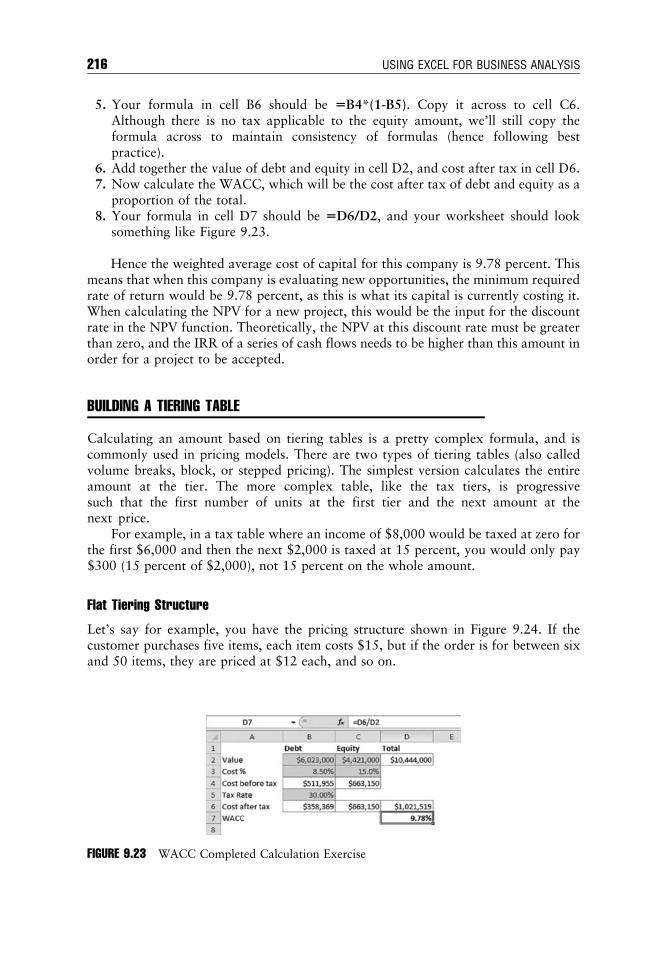
5. Your formula in cell B6 should be 5B4*(1-B5). Copy it across to cell C6.Although there is no tax applicable to the equity amount, we’ll still copy theformula across to maintain consistency of formulas (hence following bestpractice).

6. Add together the value of debt and equity in cell D2, and cost after tax in cell D6.7. Now calculate the WACC, which will be the cost after tax of debt and equity as a

proportion of the total.8. Your formula in cell D7 should be 5D6/D2, and your worksheet should look

something like Figure 9.23.

Hence the weighted average cost of capital for this company is 9.78 percent. Thismeans that when this company is evaluating new opportunities, the minimum requiredrate of return would be 9.78 percent, as this is what its capital is currently costing it.When calculating the NPV for a new project, this would be the input for the discountrate in the NPV function. Theoretically, the NPV at this discount rate must be greaterthan zero, and the IRR of a series of cash flows needs to be higher than this amount inorder for a project to be accepted.

BUILDING A TIERING TABLE

Calculating an amount based on tiering tables is a pretty complex formula, and iscommonly used in pricing models. There are two types of tiering tables (also calledvolume breaks, block, or stepped pricing). The simplest version calculates the entireamount at the tier. The more complex table, like the tax tiers, is progressivesuch that the first number of units at the first tier and the next amount at thenext price.

For example, in a tax table where an income of $8,000 would be taxed at zero forthe first $6,000 and then the next $2,000 is taxed at 15 percent, you would only pay$300 (15 percent of $2,000), not 15 percent on the whole amount.

Flat Tiering Structure

Let’s say for example, you have the pricing structure shown in Figure 9.24. If thecustomer purchases five items, each item costs $15, but if the order is for between sixand 50 items, they are priced at $12 each, and so on.

FIGURE 9.23 WACC Completed Calculation Exercise

c09 22 June 2012; 18:35:19


We’d like to populate Figure 9.24 to calculate how much a customer would becharged at different volumes.

A horribly long and complicated IF statement will do the trick:

5IF(A3,F3,G3,IF(A3,F4,G4,IF(A3,F5,G5,IF(A3,F6,G6,G7))))

But there is a much simpler way, using a VLOOKUP or LOOKUP.

1. In cell B3, calculate the per-unit price using a close-match VLOOKUP. Yourformula should be 5VLOOKUP(A3,$E$3:$G$7,3). Note that the last field isomitted, which means it will return a close match, not an exact match. You mayalso use the formula 5VLOOKUP(A3,$E$3:$G$7,3,TRUE), which will give thesame result.

2. Multiply the unit price by the number of units and add them up. Your total shouldbe $7,564, and your sheet should look something like Figure 9.25.

FIGURE 9.24 Flat Tiered Pricing Calculation

FIGURE 9.25 Completed Flat Tiered Pricing Calculation

c09 22 June 2012; 18:35:20


TIP

Because we need a close match, not an exact match, we could have used the LOOKUPfunction instead. This has the added advantage of not having to have the criteria to theleft of the result because LOOKUPs are able to search backward. You also do not haveto worry about someone inserting or deleting columns in the source data range andmessing up the formula. For more detail on how to use LOOKUPS and VLOOKUPs,see “Lookup Formulas” in Chapter 6.

Progressive Tiering Structure

If the tiering calculation is not as straightforward as the one in Figure 9.26, we mayneed to calculate under a progressive tiered structure. A good example of this is the waythat the tax calculations work, as shown in Table 9.1. This formula calculation is notfor the faint-hearted, so unless you specifically need to calculate a progressive tieringtable, feel free to skip this section.

The first person’s salary is $123,120, which means that this person is in the$80,000 to $180,000 tax bracket. However, we can’t do a flat tiering calculation onthis because the first $6,000 is tax-free, the next $40,000 is only taxed at a rate of 15percent, and so on. The formula in column I takes care of the calculations below thethreshold. Note that the tiers begin with one cent (e.g., $6,000.01).

FIGURE 9.26 Progressive Tiered Calculation

TABLE 9.1 Progressive Tiering Tables

Salary: $123,000

2010/2011 Withholding Tax Tiers Tax Rate Tax Due

0�6,000 0% 06,001�37,000 15%37,001�80,000 30% 4,65080,001�180,000 37% 17,550180,001þ 45% 54,550

Lowest Tier $80,000 $17,550$43,120 337%¼ $15,954

Total Salary $123,120 $33,504

c09 22 June 2012; 18:35:20


You’ll need to split your calculation into several parts, as shown in the diagramabove. Firstly work out the lowest tier, and then calculate the difference between thesalary and the tier (in this case $80,000). Then the remainder should be calculated atthe marginal tax rate.

Hint: This calculation will be easier if you calculate these in separate cells, and thencombine them at the end—just like we have done with previous examples of nestedfunctions, such as INDEX/MATCH or VLOOKUP/COLUMN.

1. Start by using a close match VLOOKUP to pick up column I (the amount payableup to the threshold). Your formula should be 5VLOOKUP(C2,$F$2:$I$6,4).

2. Next, we need to work out the amount over the total salary that is above thelowest tier (in this example, $123,120 � $80,000¼ $43,120). To do this we’ll doanother close match VLOOKUP returning the first column and subtract this fromthe salary amount. In a separate cell, your formula should be 5C2-VLOOKUP(C2,$F$2:$F$6,1). Your answer should be $43,120.

3. Next, we need to find out how much to multiply the $43,120 by (i.e., the highesttax tier). To do this, create a VLOOKUP returning the third column. Your formulashould be VLOOKUP(C2,$F$2:$H$6,3). Your answer should be 37 percent.

4. Now, put all three formulas together like this: 5VLOOKUP(C2,$F$2:$I$6,4)1(C2-VLOOKUP(C2,$F$2:$F$6,1))*VLOOKUP(C2,$F$2:$H$6,3).

The good news is that if you’ve used cell referencing correctly, you can simplycopy the formula down. See Figure 9.27.

MODELLING DEPRECIATION METHODS

How we treat capital expenditure, its effect on cash flow, and the subsequent depre-ciation is an important part of financial modelling—especially if your model includes aP&L statement, cash flow, and balance sheet. Capital expenditure is recorded in sev-eral different places:

FIGURE 9.27 Completed Progressive Tiered Calculation

c09 22 June 2012; 18:35:20


1. In the cash flow in the period in which it was purchased.2. On the balance sheet as a fixed asset.3. On the P&L statement as depreciation over the useful life of the asset.

In this section, we will focus on translating a purchase of a fixed asset into adepreciation charge to be shown on the P&L.

Why Depreciate?

The definition of a fixed asset is an asset that is used in production, or that supportsbusiness activities in some other way. Common examples are machinery, vehicles, andequipment such as computer hardware. Fixed assets, by definition, have an expecteduseful life of more than twelve months, and the cost of these assets must therefore bewritten off as an expense over the period in which they are used. Depreciation is thecharge calculated to write off these assets over their expected useful lives.

In the examples that follow, in Year 1 we purchase a piece of machinery for$200,000 that has a useful life of five years (i.e., it will be generating income for thenext five years), as shown in Table 9.2.

Instead of expensing the whole cost in Year 1, we should spread the cost of it overthe five years, as this is a much more accurate method of showing the profitability ineach year.

Adjusting depreciation is an attractive way for companies to increase expenses andlower taxable earnings, and for this reason, the regulatory legislation around whichmethod of depreciation can be used is strictly monitored by the tax office. Bear in mindthat finance and accounting rules differ between countries. Financial modellers do notneed to be accountants, but they do need to ensure that accounting, tax, and financerules are applied correctly if the calculation method is material to the model.

Depreciation Methods

In the example above, we have used the most common form of depreciation, which isthe straight-line method. Under this method, the cost is equally spread over the numberof years it is in use. However, there are several more complex depreciation methodsalso in use. It can be calculated either by using both a fixed rate and a fixed depreci-able base value, or by varying one or both of these variables. For this reason, the

TABLE 9.2 Depreciation for a $200,000 Piece of Machinery

Year 1 Year 2 Year 3 Year 4 Year 5

Sales $150,000 $160,000 $170,000 $180,000 $190,000Machinery ($200,000)Net Income ($50,000) $160,000 $170,000 $180,000 $190,000

Year 1 Year 2 Year 3 Year 4 Year 5

Sales $150,000 $160,000 $170,000 $180,000 $190,000Machinery ($40,000) ($40,000) ($40,000) ($40,000) ($40,000)Net Income $110,000 $120,000 $130,000 $140,000 $150,000

c09 22 June 2012; 18:35:21


depreciation charge each year as calculated by the different methods will not be thesame. Figure 9.28 illustrates the charges each year.

The exercise below will show step by step how to calculate depreciation usingthe different methods, and by doing this, we’ll see how very different each of themethods are. This is not an exhaustive list of depreciation methods; rather it’s anoverview of the most common forms of depreciation calculations used in financialmodelling.

Straight-Line Method (=SLN Function) Straight-line depreciation (also called prime costmethod) is the simplest and most-used technique that calculates depreciation at a fixedrate over the expected useful life of an asset. We estimate the residual value (salvage orscrap value) of the asset at the end of its useful life and will expense a portion oforiginal cost in equal increments over that period. The salvage value is an estimateof the value of the asset at the time it will be sold or disposed of, but often it is zero. Ifthe asset is expected to have a salvage value at the end of its useful life, we need to takethe salvage cost away from the base before depreciating it. The formula for calculatingdepreciation is therefore:

ðcost � salvageÞ=expected useful life

For example, we purchase an asset for $50,000, its useful life is 10 years, and wethink we can sell it for $5,000 at the end of its useful life. We’d simply calculatethe amount to be depreciated, which is the cost of the asset minus the residual value($50,000� $5,000 ¼ $45,000) and divide it by 10, so the depreciation amount on theP&L would be $4,500 per year for 10 years.

It’s pretty easy to work this method of depreciation by using this sort of formula:5(50000�5000)/10, or you could use the SLN formula: 5SLN(50000,5000,10),which will deliver the same result.

$12,000

$10,000

$8,000

$6,000

$4,000

$2,000

$0

2013

2014

2015

2016

2017

2018

2019

2020

2021

2022

Straight-Line (SLN)

Fixed Declining (DB)

Double Declining (DDB)

Sum-of-the-Years-Digits (SYD)

FIGURE 9.28 Comparison of Different Depreciation Methods

c09 22 June 2012; 18:35:21


Calculating depreciation using the straight-line method is by far the most commonmethod of calculating depreciation in financial modelling.

In order to demonstrate the comparison of the different methods, let’s take a lookat Figure 9.29, which shows an asset that has a purchase price of $50,000, a salvagevalue of $5,000, and a useful life of 10 years.

To prepare a depreciation schedule for this asset in Excel using the straight-linemethod, the following steps are followed:

1. Using an SLN formula, calculate the depreciation per year in row 11 columnsB to K.

2. Your formula in B11 should be 5SLN($B$5,$B$6,$B$7). This formula requirescost value, salvage value, and life in years.

3. Once the absolute value signs have been added, the formula in B11 can be copiedacross into columns C to K. Using the straight-line method, the depreciationcharge for each year is the same.

4. The amount in each year should be $4,500. After completing the table, check thatthe total is equal to cost less salvage value.

NOTE

Unlike the other depreciation methods functions, the SLN function does not stop when it has fullydepreciated the asset. If you continue to copy row 11 across to cell K11, you will notice that it continuesto apply depreciation, even though the asset has been fully depreciated. If you have assets being fullydepreciated during the life of the model, this will need to be calculated manually if using the straight-linemethod. See “Calculating Depreciation at the End of Useful Life” later in this chapter for how to calculatedepreciation on assets that have been fully depreciated.

Declining Balance Value Methods

These methods are also called the reducing balance, diminishing value, or acceleratedmethods. You could argue that assets are more useful when they are new, and thereforedepreciate more quickly in the first few years of acquisition. Therefore, some compa-nies use depreciation methods that provide for a higher depreciation charge in the firstyear of an asset’s life and gradually decrease charges in subsequent years. These arecalled accelerated depreciation methods.

FIGURE 9.29 Asset Depreciation Example

c09 22 June 2012; 18:35:21


Fixed Declining Balance Method (=DB Function) The fixed declining balance method cal-culates depreciation at a fixed rate. This rate is calculated by the formula:

1� ((salvage/cost)^(1/life))

But it’s much easier using the ¼DB Excel function! The depreciation charge foreach period is not the same, as the depreciation rate for a period is applied to the netbook value at the beginning of that period, and not to the original cost. With thismethod, the starting net book value is the cost price, so depreciation is applied to costand not the value of cost less salvage. This is because using this method, the net bookvalue can never reach zero.

Instead of treating each year the same, the fixed declining method depreciates morequickly in early years and more slowly in later years. The book value of the asset at thebeginning of the period is multiplied by a fixed rate (e.g., in Year 1, 10 percent of$45,000 is $4,500 of depreciation). In Year 2, the same 10 percent is multiplied by theremaining $40,500 of book value, which then gives a depreciation value of $4,050.

The most difficult part in the fixed declining method is to figure out the correctpercentage to use for each year, which is done with a rather complicated algebraicformula. If you use the pre-defined DB function in Excel, however, you don’t need to beconcerned with the calculations. Bear in mind, however, that when Excel calculates therate, it rounds to three decimal places, and this does cause the calculation to be off by afew dollars at the end of the useful life.

Therefore, unlike the straight-line method, you pretty much have to use the Excelformula. Using the example above, your fixed declining formula for Year 1 would looklike this: 5DB(50000,5000,10,1).

Applied to the example above, to prepare a depreciation schedule for a particularasset on Excel using the fixed declining balance method, the following steps arefollowed:

1. Using a DB formula, calculate the depreciation per year in row 12, columns B to K.2. Your formula in B12 should be 5DB($B$5,$B$6,$B$7,B10). This formula

requires cost value, salvage value, life in years, and period for which depreciationis being calculated.

3. Note that the additional requirement of a specified period is a result of thedepreciation calculated each year being unique to that particular year, or period.For this formula to return an accurate result, both life and period must be enteredusing the same unit (e.g., years).

4. Once the absolute value signs have been added, the formula in B12 can be copiedinto columns C to K.

5. If you create a total in L12, this will not be exactly equal to cost less salvage, aswas the case for the straight-line method. This is a result of the fixed decliningbalance method producing a hyperbolic function and not a linear function and,therefore, never allowing the net book value to be zero.

6. Once the table has been completed, check that the total calculated in L13 is notmore than cost less salvage. If this is the case, a manual adjustment to the lastperiod’s depreciation charge will be required.

Your worksheet should look something like Figure 9.30.

c09 22 June 2012; 18:35:21


Double Declining Balance Method (=DDB function) The double declining balance methodalso calculates depreciation at a fixed rate. This rate per annum is calculated as:

(23 (100/expected useful life)) %

Again, the Excel function (=DDB) makes this calculation a lot easier!As with the fixed declining balance method, the depreciation charge for each

period is not the same. This is a result of the depreciation rate being applied to the netbook value at the beginning of each period, and not to the original cost. Here, too,the starting net book value is the cost price and not cost less salvage. This method isquite similar to the fixed declining method shown above, except that the first year’sdepreciation uses double the percentage of the straight-line method. For each addi-tional year of the asset’s life, opening book value is multiplied by the same per-centage. When the amount calculated by the double declining method is less thanwhat it would have been using the straight-line method, then the straight-line methodis used.

In the example above, using the double declining balance method, the depreciationrate would be 20 percent in the first year instead of 10 percent using the straight-linemethod. This amount then reduces until it is less than $5,000, and then it switches tothe straight-line method.

Again, using the followingExcel function is recommended:5DDB(50000,5000,10,1).To prepare a depreciation schedule for a particular asset on Excel using the double

declining balance method, the following steps are followed:

1. Using aDDB formula, calculate the depreciation per year in row 13, columns B to K.2. Your formula in B13 should be 5DDB($B$5,$B$6,$B$7,B10). This formula

requires cost value, salvage value, life in years, and period for which depreciationis being calculated.

3. Once the absolute value signs have been added, the formula in B13 can be copiedinto columns C to K.

4. Once again, the total in L13 will not be exactly equal to cost less salvage, as wasthe case for the straight-line method. This is a result of the double declining bal-ance method also producing a hyperbolic and not a linear function.

5. Once the table has been completed, check that the total calculated in L13 is notmore than cost less salvage. If it is, a manual adjustment to the last period’sdepreciation charge will be required.

FIGURE 9.30 Calculating Fixed Declining Depreciation

c09 22 June 2012; 18:35:21



Sum-Of-The-Years’-Digits Method (=SYD Function) Unlike the previous three methods ofcalculating depreciation, the sum-of-the-years’-digits (SYD) method calculates deprecia-tion at varying rates for each period. As with the straight-line method, however, it uses aconstant depreciable base, being cost less salvage value. The sum-of-the-years’-digits iscalculated as:

ðnðnþ 1ÞÞ=2where n is equal to the useful life in years.

Depreciation for each period is then calculated as:

ðcost � salvageÞ3 ðuseful life� number of previous periodsÞ3 sum-of-the-years’-digits

Sum-of-the-years’-digits is a depreciation method that results in a more acceleratedwrite-off than straight line, but less than the declining balance method. Under thismethod, annual depreciation is determined by multiplying the depreciable cost by aschedule of fractions.

Use the Excel formula 5SYD(50000,5000,10,1).To prepare a depreciation schedule for a particular asset on Excel using the sum-of-

the-years’-digits method, the following steps are followed:

1. Using an SYD formula, calculate the depreciation per year in row 14, columns B toK.2. Your formula in B14 should be 5SYD($B$5,$B$6,$B$7,B10). As with the pre-

vious two methods, this formula requires cost value, salvage value, life in years,and period for which depreciation is being calculated.

3. Once again, the additional requirement of a specified period is a result of thedepreciation calculated each year being unique to that particular year, or period.Unlike with the two previous methods however, the difference in yearly deprecia-tion charges is a result of a change in rate, and not a change in the depreciable base.

4. Once the absolute value signs have been added, the formula in B14 can be copiedinto row 14, columns C to K.

5. Check that the total in L14 is, as with the straight-line method, exactly equal tocost less salvage value. Despite using varying rates, this method also produces alinear function.

FIGURE 9.31 Calculating Double Declining Depreciation

c09 22 June 2012; 18:35:22


Your worksheet should look something like Figure 9.32.Of course, there are many other methods of depreciation, most of which also have

an Excel function, to make what would otherwise be an extremely complicatedcalculation much easier. Don’t completely rely on the function, however! As always,sense-check the results and double-check the timing of the purchase date and the periodat which the asset is deemed to be fully depreciated.

Calculating Depreciation at the End of Useful Life

When building a model to depreciate assets using the straight-line method, whethercalculating it longhand, or using the SLN function, it is possible to continue to calculatedepreciation on an asset that has already been fully depreciated past its useful life. Thisresults in an ever-increasing negative net book value, which is impossible, and can bethe cause of an error in the model.

In order to prevent depreciation from being calculated once the asset has reachedthe end of its useful life, the Excel depreciation formula needs to be amended.

Let’s say you have a list of capital items in a database, as shown in Figure 9.33. Thefirst item on the capital expenditure register is for some IT equipment that was pur-chased in July 2011. The useful life is three years, which means that it will be fullydepreciated in July 2014, and therefore if we create a forecast model for 2014, we needto ensure that the depreciation does not continue past the end of its useful life, and weneed to create a formula to do this. See Figure 9.33.

FIGURE 9.32 Calculating Sum-Of-The-Years’-Digits Depreciation

FIGURE 9.33 Assets Register

c09 22 June 2012; 18:35:22


This will be a rather long formula, but we’ll use a simple building block meth-odology where we create a simple formula, test it, and check it before adding to it. Wethen test and check it again, before adding to it. In this way, we minimise errors bymaking sure the formula syntax is correct.

1. Begin by calculating the depreciation for January 2014 for the asset in cell G4,using the straight-line depreciation method. Remember it’s for a month, not a year.Your formula should look like this: 5SLN($D4,$E4,$C4)/12.

Test this by copying across and down the page to make sure that the cellreferencing is correct.

2. Once we’ve got this right, we need to consider the spend date. In some instances,the spend date for the item has not yet elapsed, so we need to evaluate whether thisdate has passed or not, and only allow the depreciation to show if the date haspassed. We can achieve this by inserting an IF statement around the SLN functionlike this: 5IF(G$2.5$B4,SLN($D4,$E4,$C4)/12,0). Test this by copying acrossand down the page to make sure that the cell referencing is correct.

3. Now we need to consider the end-of-useful-life date. We could do this all in oneformula, but it will make our calculations easier to follow if we insert this as a datewithin the model. In cell F4, calculate the date at which the item will be fully depre-ciated.We can do this using the formula5B41(C4*365). However, note that it givesyou a value of June 30, 2014, because 2012 is a leap year. You can get around this byusing the EOMONTHorDATE functions or by using 365.25 instead of 365—or youcan simply leave it as it is. Copy the formula down column F.

4. Next,we need to add in the end-of-useful-life date to our formula in cell G4. The bestway to do this is by adding the AND function using the syntax. Your formula shouldlook like this: 5IF(AND(G$2,5$F4,G$2.5$B4),SLN($D4,$E4,$C4)/12,0).

5. Copy the formula across and down, and test to see if it is working correctly. Thedepreciation for the IT equipment should stop in July 2014.

6. Your worksheet should look something like Figure 9.34.

BREAK-EVEN ANALYSIS

Including break-even analysis in a financial model is very useful for budgeting purposesand especially for any business that is starting or expanding its operations. Break-evenanalysis is a very effective tool to determine profitability and give you a snapshot of the

FIGURE 9.34 Completed Depreciation Calculation on Fixed Assets

c09 22 June 2012; 18:35:22


sales volume target that is required to start making profit. For a new start up venture,this analysis is very effective in projecting sales targets. For established companies thatare looking to launch new products and services, this analysis is invaluable in devel-oping the pricing strategy.

There are several different ways to carry out the break-even analysis, depending onthe perspective you want to look at. If you keep your pricing fixed, you can determinethe units you need to produce and sell to break even (zero profit and zero loss). On theother hand, if your market position allows you to change the pricing, then you candetermine the optimal pricing strategy to make your department or business break evenwithin the stipulated target sales.

Let’s take an in-depth look at some of the different methods of calculations forbreak-even analysis. It is also very helpful to show break-even points graphically so wewill also include some line charts when calculating the break-even points in our modelin this section.

Calculating Break-Even Point

The break-even point is dependent on the total cost of production, the price of units,and the number of units. In its most simplified form, the break-even point is achievedwhen:

Total cost of production ¼ price3 number of units

However, in real businesses the equation is not this simple because the cost ofproduction is never completely fixed. There is a variable component to it, which isrelated to the total units produced. This component includes everything from the priceof raw materials, labor costs, and additional overheads. Thus total cost of production isthe sum of the fixed costs and the variable costs.

Total cost of production ¼ fixed costs þ variable costs

By varying the total number of units and/or the selling price of each unit, you cancalculate thebreak-evenpoint for yourbusiness. Figure 9.35 showsanexample the variousbreak-evenpoints at three differentpricepoints: $100,$150, and$200.Wecan see that thelower the selling price per unit, the more units we need to sell in order to break even.

Example Using Excel

Let’s look at an example of how to calculate the break-even point for a new pro-duct. Let’s say you want to start producing custom-made birdcages. You have deter-mined your fixed and variable costs for the first year are as follows:

n Fixed costs $250,275 (this includes rent, machinery, electricity, etc.).n Raw materials of $5 per cage.n Labour of $25 per cage.n Overheads of $10 per cage.

Using the layout in Figure 9.36, calculate the net profit at each level of production.Ensure you use consistent formulas! At what level of production does the businessbegin to make a profit? The answer follows in the numbered list.

c09 22 June 2012; 18:35:22


1. Fixed costs will remain $250,275 regardless of the production level. The formulain cell F5 should be 5$C$3. Copy it across.

2. Variable costs will fluctuate depending on the volume produced. The formula incell F6 should be 5F4*$C$8. Copy it across.

3. Add together the fixed and variable costs in row 7.4. Calculate the total revenue in row 8. The formula in cell F8 should be 5F4*$F$3.

Copy it across.5. Now calculate the net profit at the various production volumes in row 9.6. The formula in cell F9 should be 5F8-F7. Copy it across.


$600,000

$500,000

$400,000

$300,000

$200,000

$100,000

$00 1,000 2,000

Bob’s Bird Cages Break-Even Analysis

3,000 4,000

Fixed costTotal costRevenue

FIGURE 9.35 Break-Even Chart

FIGURE 9.36 Break-Even Example Layout

FIGURE 9.37 Break-Even Calculations

c09 22 June 2012; 18:35:22


We can see that somewhere between 2,000 and 3,000 cages is when the revenuebegins to cover our costs.

Charting the Break-Even Point

It is also interesting to look at the numbers graphically, and we can create a line chartthat shows the point at which the revenue from the business becomes greater than thecost. See Figure 9.38.

For detailed instructions on how to create this chart, see the supplementarymaterial available on www.wiley.com/go/steinfairhurst.

We can see what the break-even point is by looking at the chart, but it can be apretty laborious task when done manually, and it is also not very accurate. We cancalculate this exactly, however, using two methods:

1. A formula calculation.2. A goal seek.

Calculating Break-Even Using a Formula

Using a formula is the fastest way of calculating the break-even point. It can be cal-culated using the following formula:

fixed cost

price� variable cost

Price minus variable costs gives you the gross profit, or contribution of each unit.We can then divide the fixed costs by the contribution to see how many units need to besold to cover the fixed costs. See Figure 9.39.

Fixed costTotal costRevenue

$600,000

$500,000

$400,000

$300,000

$200,000

$100,000

$00 1,000 2,000 3,000 4,000

Bob’s Bird Cages Break-Even Analysis

FIGURE 9.38 Completed Break-Even Chart

c09 22 June 2012; 18:35:23



In our model, we can calculate the break-even point by using this formula:

$250; 275

$125� $40¼ 2; 944:41

The Excel formula in our model to calculate this is:

C5/(C11�C10)

Break-Even Analysis Using Goal Seek

Another way to perform a break-even analysis is to use the goal seek tool. For arefresher on how to use this tool refer to the “Goal Seeking” section in Chapter 8.While this method takes a little longer to set up and run than using a formula asdescribed above, it is more flexible and allows more options for changing inputs.

Using our Bob’s Birdcage example, we need to set up the sheet as a simple P&Lcalculation, as shown in Figure 9.40.

The number of cages produced is the unknown variable, and we have entered avalue of 2,500 into cell C11 as a placeholder in the meantime (which we can seegenerates a loss). This is the variable that will change when we perform the goalseek. Remember that to perform a goal seek we need a formula, and a hard-codednumber that drives that formula. The formula will be the profit/loss amount in cellC16, and the hard-coded number is the number of cages in cell C11. Make sure thatall of the formulas in cells C13 to C16 contain formulas; otherwise the goal seekwon’t work.

So to perform the break-even analysis, we need to set the net profit/loss value tozero by changing the number of cages produced. See Figure 9.41.

When you click OK, Excel calculated the exact breakeven point and edits the cellvalue accordingly, as shown in Figure 9.42.

We can see that we end up with a value of 2944.41176470588. You might like toround it to the nearest unit, which will show a small profit or loss, which might beconfusing. Alternatively, change the formatting so that the decimal places don’t show.

FIGURE 9.39 Break-Even Number of Units Using a Formula

c09 22 June 2012; 18:35:23


FIGURE 9.40 Setting up a Break-Even Calculation for Goal Seek

FIGURE 9.41 Using Goal Seek to Calculate Break-Even Point

FIGURE 9.42 Completed Break-Even Goal Seek

c09 22 June 2012; 18:35:23


If you have the power to manipulate the unit pricing, then you can change the pricepoints to reach breakeven at the sale of fixed number of units, and even set profittargets using the goal-seek function. Let’s say you don’t think you can sell more than2,500. What would you need to set your price at in order to make a profit of $50,000 ifthe maximum you will sell is 2,500? Because of the way we have set up this model, thisis relatively easy to calculate. See Figure 9.43.

If we want to make a profit of $50,000, we’d need to sell 2,500 cages at $160 each.Whilst the goal-seek method takes a little longer to run and set up, it’s a great way

to run different scenarios and test changes in inputs when performing breakevenanalysis.

SUMMARY

In the first part of this book, we covered the tools, functions, and techniques thatfinancial modellers need to know. In this chapter, we focussed on the use of these toolsin a financial modelling context. If you are pursuing a career as a financial modeller,you will almost certainly have to calculate escalation at some point, and it is quite likelythat you will find yourself needing to use tiering tables, calculate depreciation, orperform a break-even analysis.

FIGURE 9.43 Break-Even Goal Seek with Changed Inputs

c09 22 June 2012; 18:35:23


c09 22 June 2012; 18:35:24

CHAPTER 10Model Review

I f you are lucky, you will get to build your own model from scratch, but most oftenyou will be handed someone else’s model to validate, modify, and make your own.

One of the toughest tasks for any financial modeller is trying to use, understand, audit,or validate an existing model. While it may seem like a simple enough task where thehard work is already done, the real challenge will be to understand how the model wasdesigned.

Excel is such a flexible tool, and there are so many different ways to achieve thesame end, that trying to understand the way a model has been built is like trying to getinside another modeller’s mind! Give three different modellers a problem, and you’llundoubtedly have three different model designs, as each modeller will approach themodel design in a different way and almost certainly using different formulas.

REBUILDING AN INHERITED MODEL

Obviously the best place to start when trying to understand a model is to talk to theoriginal designer, if that is at all possible. There is no one who understands the modelbetter than the modeller who designed it in the first place. However, the originalmodeller is often unavailable, and we therefore need to allow the model to speak foritself.

If financial modelling best practice has been used, understanding a financial modelin Excel should be a fairly straightforward task. However, many inherited models havenot been built by professional modellers, but rather cobbled together by different areasof a business to achieve a (usually short-term) outcome. These kinds of inheritedmodels can be a real nightmare to unravel, and often it’s simply easier to start fromscratch. If this is not practical, there are some tricks and techniques in Excel thatcan help you to take apart someone else’s model. Using these techniques you canmake the task of rebuilding an inherited model more achievable. We will explore someof these techniques in this section.

Removing Redundant Assumptions and Source Data in a Model

Common problems modellers encounter when rebuilding an inherited model areredundant assumptions and sources in the data model. This can happen when mod-ellers need to use source information that is already in the spreadsheet, and re-createwithout realising that they are entering a duplicate set of assumptions or data. Often as

c10 22 June 2012; 18:43:22

235

a model evolves, parts of the model calculations are deleted, but the assumptions thatfed into those calculations remain, despite no longer being needed.

The easiest way to see if any formulas are linking to an input cell is to use the tracedependents formula-auditing tool. This tool will allow you to trace forward andbackward throughout the model. One technique you can use to remove redundant cellsis to colour code all of the input assumption and calculation cells. Then go to the modeloutputs, and trace back the formulas. As each input assumption is validated, change thecolour of the input cells back to their original colour. At the end of the process, if anycells are still coloured, you will know that they are redundant and can be deleted.

If you think a section of the model is not being used, check it using the tracedependents formula-auditing tool as described in this chapter before deleting it. Beaware that there are a few tools and formulas such as INDIRECT and OFFSET thatsometimes can rely on a cell but that do not show up in the formula auditing tool. Forthis reason, make sure you save before deleting, and check the output of the model for#REF! or other errors before continuing. If the deletion has caused a problem, you cansimply undo or close without saving to revert to the version of the file prior to deletion.It’s also best to delete entire rows or columns instead of just clearing cells whenremoving sections of a model in this way. Deleting the cell will show an error and flagthe issue if it had been linking to a formula, whereas clearing cells will simply changethe value to zero, which will not necessarily return an error. This can cause undetectederrors to remain in the model.

Formula Auditing

One of the most effective ways to start understanding a financial model (especially onethat you did not build yourself!) is to look at the formulas and identify the precedentsand dependents. This will give you an idea of the logic used by the previous builder ofthe model. Usually the best place to start in this technique is the final output. Take alook at each output and trace back the predecessors until you eventually find out whatcalculations, source data, and assumptions have been used by the original designer.

If you have a formula and you want to know which cells it uses, the easiest way isto use formula auditing. You can access these features in Excel from the FormulaAuditing ribbon under the Formulas tab, as shown in Figure 10.1.

Tracing Precedents To trace the precedents, select the cell you want to audit and clickon Trace Precedents in the Formula Auditing ribbon. See Figure 10.2. (See the Excel2003 instructions available at www.wiley.com/go/steinfairhurst.)

The trace precedents feature allows you to see all the other cells whose values areused in the formula in the present cell. It is possible to understand the calculation justby observing the cell formula too, but the arrows make it easier to locate the cells,which reduces the chances of errors in auditing the model. See Figure 10.3.

FIGURE 10.1 Formula Auditing Icons in the Ribbon

c10 22 June 2012; 18:43:23



NOTE

Double-clicking on the blue arrows will take you to the preceding cells. If you double-click again, it willbring you back to the original cell. Also note that if the preceding cells are on another page, the blue arrowwill show a dotted line. To go to the precedent cell, simply double-click on the dotted line, and it will bringup a list of all the off-sheet references of that cell. Double-click on the reference to go to that cell.

Tracing Dependents Just like precedents, you can also trace the dependents to a particularcell. These are all the cells that use the value in the current cell for the calculations.

Select the Trace Dependents button in the Formula Auditing ribbon under theFormulas tab. See Figure 10.4.

This is particularly useful if you are considering deleting a cell and don’t want tomess up the model. (See the Excel 2003 instructions available at www.wiley.com/go/steinfairhurst.)

FIGURE 10.2 Trace Precedents in Excel 2007/10

FIGURE 10.3 Using Trace Precedents on a Formula

c10 22 June 2012; 18:43:23

Model Review 237



TIP

Click on the Trace Precedents button again to trace the precedents of the precedentcells. This is invaluable in auditing complex formulas.

While arrows are great visual aids to understand the formula, sometimes they canbecome a distraction, especially if there are too many of them. You can clear all thearrows by clicking on the Remove Arrows button. See Figure 10.5. This is also

FIGURE 10.4 Trace Dependents in Excel 2007/10

FIGURE 10.5 Removing All Arrows

c10 22 June 2012; 18:43:23


important if you plan to print the spreadsheet. If you don’t remove the arrows beforeprinting, they will show up on the printed document.

NOTE

There are some formulas upon which the Formula Auditor will not work very well, such as array formulas,data tables, and the INDIRECT formula. These are visible using the Dependency Auditor tool, which canbe purchased separately from Microsoft.

TIP

You can also jump to precedent cells by using these shortcuts:

n Control þ [ (open square bracket) to jump to and highlight precedent cells.

n Control þ ] (close square bracket) to jump to and highlight dependent cells.

These shortcuts can be performed in Excel for Mac 2011 by using the Commandinstead of Control key.

Error-Checking Tools There are times when we unintentionally introduce errors in thefinancial model. This could be because we did not comprehend the logic completely orbecause we mistyped the formula. Excel provides an error-checking function that helpsidentify the problem. This is extremely useful when your incorrect formula is syntac-tically correct. Excel indicates the anomalies in the model with a green triangle in thetop-left corner of the cell.

To understand the nature of the error, select the cell and click on the drop-downmenu. There are many categories of such errors, but inconsistent formula is one of themost common errors, as is omitting adjacent cells, as shown in Figure 10.6

You can change the kind of error checking you want to perform on your model byselecting the Error Checking Options, as shown in Figure 10.7. This will display thescreen where you can control the kind of checks you want performed.

You can also access the Excel Options dialog box from selecting the File tab orMicrosoft Office button, then Options or Excel Options. In Excel for Mac 2011, accessExcel Options by clicking Excel, then Preferences, then Error Checking.

You can review all the errors in the financial model using the error checking featurein Excel. See Figure 10.8.

Error checking offers two options:

1. Error Checking: Used to check formulas in error.2. Trace Error: This is used to trace the source of the error in the final result. To use

this feature, select the cell with the error (usually shown as #ERR?, #NAME?, etc.)and click on Error Checking—Trace Error. See Figure 10.9.

Excelwill trace back the source of the errorwith a red arrowas shown inFigure 10.10.

Evaluating Formula Tool Sometimes it is difficult to decipher a complex nested formulajust by looking at precedents and dependent relations. It is easier to actually evaluate it

c10 22 June 2012; 18:43:24

Model Review 239

FIGURE 10.7 Editing Error-Checking Options

FIGURE 10.6 Error-Checking Tools Showing Error in Sum Formula

c10 22 June 2012; 18:43:24


step-by-step to understand how it works. Excel facilitates this by the use of the EvaluateFormula feature.

To evaluate a formula in any cell, select the cell and click on Evaluate Formula inthe Formula Auditing ribbon under the Formula tab. See Figure 10.11.

This will display an Evaluate Formula dialog that will show you the completeformula in the cell. Keep clicking on the Evaluate button to see how Excel calculates thevalue step-by-step. See Figure 10.12.

Once you have looked up the source of the parameter, you can click Step Out tocontinue the evaluation.

NOTE

The Evaluate Formula auditing option is currently unavailable for Excel for Mac 2011.

FIGURE 10.9 Error-Checking Options

FIGURE 10.10 Tracing the Error Source

FIGURE 10.8 Error-Checking Feature

c10 22 June 2012; 18:43:24

Model Review 241

FIGURE 10.11 Evaluate Formula in the Ribbon

FIGURE 10.12 Evaluate Formula Dialog Box

TIP

You can also evaluate a partial formula manually by selecting each expression andpressing F9. You must select an entire section of the formula that makes sense in itsown right; for example, in the horribly long and complex formula shown in Figure10.13, we can select this portion of the formula: SUM(B$2:B2).

FIGURE 10.13 Selecting Part of the Formula

By then pressing F9, the formula will display the result of that expression, which inthis case is 250. See Figure 10.14.

c10 22 June 2012; 18:43:24


NOTE

The Evaluate Formula auditingoption and the related shortcut are currently unavailable for Excel forMac 2011.

Viewing All the Formulas If you want to look at all the formulas and not the evaluatedvalue, you can use the Show Formulas option in Excel. This is also a very effective toolto understand the general logic in the model and can sometimes make anomalies moreevident.

This can also be done using the CTRL þ 0 shortcut key. Note that 0 is usuallylocated below the B key at the top left of the keyboard, and should not be confusedwith the CTRL þ ’ shortcut used to edit cells. See Figure 10.15. No keyboard shortcutexists at this time for Excel for Mac 2011. (See the Excel 2003 instructions availableat www.wiley.com/go/steinfairhurst.)

FIGURE 10.14 Viewing the Value of Part of the Formula

If you thenhit theEnter key, itwill paste that value into the formula (usually notwhatwe want to do) but if you hit Escape, it will return to normal. This is a handy little trickthat is sometimes easier and less complicated than using the Evaluate Formula tool.

For more detail on why you would want to break up a formula in this way, see“How Long Should a Formula Be?” in Chapter 4.

FIGURE 10.15 Show Formulas Option in the Ribbon

c10 22 June 2012; 18:43:25

Model Review 243


Direct Editing By default, Excel allows users to edit the formulas directly in the cell,when they double-click the cell. However, while auditing any inherited spreadsheet,this may not be a good idea, as we could inadvertently mess up the formulas that arealready in the cell. Excel allows users to disable direct editing, which protects the cellsto a degree, but it still allows users to view the formula. It is quite different fromprotection, which does not let you do anything at all on the cell, and it’s much easier toturn off and on than protection.

Using this tool you can double-click on the cell to trace back, and ensure that youunderstand the assumptions made by the original modeller and take care that you arenot making any inadvertent changes to the formulas in the cell. You can still make anychanges necessary directly in the formula bar.

You can disable Direct Editing from the File menu. Click Options, then Advanced,and select Allow Editing Directly in Cells. Note in Excel for Mac 2011 this option isfound in Excel . Preferences . Edit. Select Double-Click Allows Editing Directly inCells. See Figure 10.16.

Now when you double-click on the cell, it will highlight all the cells used asparameters in the formula, but not let you edit the cell directly. See Figure 10.17.

FIGURE 10.17 Direct Editing Disabled

FIGURE 10.16 Disabling Direct Editing in Cells

c10 22 June 2012; 18:43:25


AUDITING A FINANCIAL MODEL

Any model used to support output required for decision making purposes should bechecked and tested at some level by an independent party (whether internal or external tothe organisation) for both logic and accuracy before it is handed over to the end user.Reviewing, checking, and auditing a model are important parts of the model-buildingprocess.Asdiscussed in the section on financialmodelling best practice, checking shouldbedoneby themodellerduring themodelbuildprocess.However,once themodel is complete,or near completion, it should be reviewedby another party not involved in themodel build.

How detailed the audit needs to be will depend on the importance of the financialmodel to the organisation using it. Whether it’s a simple pricing model or a multi-million-dollar merger, at least some level of checking and testing appropriate to themodel need to take place in order to identify and eliminate spreadsheet error and toensure that calculations, assumptions, and logic within the model are correct. Beloware listed a few different levels of testing and audit that may be appropriate for a model.

1. Informal check: In many models this process could be an informal check by acolleague before passing it on to senior staff.

2. Quality assurance (QA) procedure: For larger projects, such as the one outlined in“Steps to Building a Model” in Chapter 2, particularly if a team is involved, it is animportant final step in the build process prior to handing over the model. Thiswould be a more formal (QA) procedure carried out and documented by themodelling team, and is also usually conducted internally.

3. Formal model audit: When a high-profile transaction, such as an acquisition orhigh-stakes project finance, an external auditing specialist will be engaged toconduct an independent audit of the financial model. These audit procedures areoften a requirement of banks, lenders, and investors as part of the due diligenceprocess to satisfy themselves that the projections and results of the financial modelare reliable and accurate.

The type of audit that needs to take place will depend on the size, scope, and impor-tance of the financialmodel youhave beenworking on. Unless youwork for amodel auditfirm, you are unlikely to be involved in an externalmodel audit, so let’s take a look at howto go about the internal checks, which you are most likely to be involved with.

Informal Check

Let’s face it; the majority of financial models built will only get an informal check bycolleagues. Depending on how much time they have available, they could spend any-thing from an hour to several weeks testing your model. Below are some techniquesthat can be used to test the integrity of the model on an informal basis.

n The traditional method of auditing is commonly known as the tick-and-bashmethod, whereby the model checker goes through the model cell-by-cell to checkfor consistency and logic. This is not a particularly effective method of checking, asit is highly likely that the tester will very quickly become bored with this tedioustask and miss anomalies. It is also a task commonly given to junior staff who oftendo not have the practical modelling experience to know common errors.

c10 22 June 2012; 18:43:25

Model Review 245

n A more effective, but more costly, method is to commission the development of aparallel model to support the primary model. This can be done by providing anindependent modeller with the input page to a model and the output layoutrequired—without the numbers. The modeller is then required to build a high-levelparallel model (minus the bells and whistles, of course). This can then be comparedto the results produced by the primary model and confirm that the primary modelis working correctly. This is a rather time-consuming exercise, but one of the mosteffective ways of checking model accuracy.

n Ditch the spreadsheet and use a calculator! Print out the results of the model andsee if you can roughly achieve the same results offline.

n Another effectivemethodof testing amodel is touse scenarios, sensitivity analysis, andstress-testing. Change the inputs to something unexpected and see what happens.If you change the price of all your products to zero, does you revenue become zeroalso? It should, and if it does not the tester needs to understand why. See “Scenariosand Sensitivity Analysis in a Business Case” in Chapter 11 for more detail on how toperform sensitivity and stress-tests.

n Create lots and lots of charts. Create metrics, and plot as many inputs and outputson the same charts as you have time for. Calculate the revenue per customer andchart it against market share on a line/column combination chart on two separateaxes. (See “Charting on Two Different Axes and Chart Types” in Chapter 12 forhow to do this.) Make sure that you understand every single trend and movementin the charts as these can flush out anomalies in the model that may not have beenvisible previously.

QA Procedure

Working on a QA procedure is the most labour-intensive type of audit most modellersare likely to be involved in. Below are some detailed instructions of how to go about afinancial model QA procedure. The QA of a model involves two main tasks:

1. Logic checking, which aims to test whether the logic underpinning the model isreflected accurately in the model. These tests check that the model does what it issupposed to do. This form of QA should be carried out once the model is com-pleted and before it is used to generate outputs. It should be repeated again later ifsignificant changes have been made to the model structure.

2. Data checking to ensure that the correct input data is used and has been enteredinto the model accurately. This type of QA may be more appropriately undertakencloser to finalisation of the report, when final decisions have been made onparameters that should be used in the model.

QA Logic Testing Step 1: Scope of the QA Work. Before you begin, the scope of the QAneeds to be established. The person undertaking the QA should clarify what parts of themodel need a QA and, in particular, whether there are any parts that need specialattention. For example, certain calculations may be crucial to the model and the modeldeveloper may want assurance that the logic of the formulas used is appropriate. Insome cases the model developer may seek feedback on possible improvements to themodel, so as to enhance transparency, clarity, or some other aspect.

c10 22 June 2012; 18:43:26


It is important to ensure that all supporting documentation is available to under-take the QA process. The model developer and/or the project team should provide allthe documentation and source data in either hard or soft copy.

Step 2: QA Checks of Calculations and Logic. Logic checks are carried out in order to:

n Check that cell referencing in a formula is consistent and correct.n Ensure that formulas are mathematically correct.n Confirm that the formulas used are suitable.n Ensure consistency within the model in relation to the use of inputs such as:

n Nominal or real values.n Units (for example, $’000,000 or $’000; kL or ML).n Timing assumptions, where applicable.n Labelling, which should be clear.

To check the logic of a model, quality assurers must first understand the output themodel is required to produce and determine if the calculations correctly produce thatoutput. Some of the tasks required in undertaking a logic check are therefore the sameas those that would be done in the model building process.

To check the calculations and logic, the following steps should be followed:

1. Understand the purpose and limits of the model. This includes ascertaining whatthe model is supposed to do, what questions the model is supposed to answer, howthe model tries to answer the questions, what the limitations of the model are, andwhat the model cannot do. This will most certainly require discussions with theproject team and model developer.

2. Stress-test the model as a whole by entering awide range of inputs and checking thatthe outputs are logical. This includes testing values at the extremes to ensure themodel processes the input as expected, especially where validation and protectionare used. While testing a wide range of combination of input variables may identifysome hidden bugs in the calculations, using 0 or 1 is a goodway to highlight obviouserrors, as the outputs should be simple. For example a unit price of zero shouldgenerate a revenue of zero, and if it does not, you’ll need to investigate why not!

Another way of testing this is to use historical figures as input and test whetherthe model can replicate actual results. For example, key outputs such as profit,growth rate, and other financial ratios that are calculated by the model can becompared to the known historical results.

Yet another way is to check the sensitivity of outputs (dependent variables) tochanges in the inputs (independent variables). This involves checking that thedirection and magnitude of the change are in accordance with how you logicallyexpect the outputs to behave.

3. Establish which cells contain formulas. This can be done using audit software suchas Spreadsheet Detective (an add-in available for purchase from Microsoft), whichallows easy identification of which cells are fully hard-coded, which contain for-mulas, and whether formulas are consistent across rows and columns.

4. Check both the logic and the reference accuracy of each identified formula. This isusually done by tracing the outputs back to the inputs to ensure that calculations

c10 22 June 2012; 18:43:26

Model Review 247

produce accurate and logical output. See the “Formula Auditing” section earlier inthis chapter for detail on how to use the Trace Precedents tool.

To assist with the logic and calculation checks, you may choose to write downthe formulas in Excel notation using cell names and also in plain English bysubstituting the cell names in the formula with the actual variable names. Forexample:

Excel notation: J25 5 J6*J9Plain English: total variable cost ¼ variable cost per unit 3 number of unitsLogic: number of units drives total variable cost

This is a simple and effective method to check and document the logic of theformula used by the model developer, and pick up any cell referencing errors.Sometimes a formula can be quite long, especially if Excel nested functions areused. Writing it out and breaking it down into its components makes it easier tothoroughly check each component (e.g., ensuring that they are referenced cor-rectly, consistent in years, units, etc.). The tool Dependency Auditor can help withthis auditing by providing the Excel notation.

5. Check that the calculations have been suitably applied. For example, an indexationformula may be correct, but may not be suitable where it is applied, if, forexample, the underlying data is already inflated.

Step 3: QA Checks of the Model’s Structural Layout and Documentation. Apart fromits underlying calculations and logic, each model’s structural layout, appearance, anddocumentation should be checked.

Checking the structural layout of each sheet and workbook involves reviewingthese to make sure that they are simple, transparent, and easily navigable. Elements tolook out for are:

n Logical sequencing of the components in the model.n Whether calculations are spread out all over the model or if they follow neatly

down and across in a logical fashion. (Note that in larger models not everythingwill follow neatly!)

n Whether hard coding is only on the input sheet.

Checking the model’s appearance and documentation involves checking thespelling and formatting, as well as that the documentation and notations in the modelare clear, are easily understood, and accurately reflect what is in the model.

Step 4: Document Your QA Work. The QA procedure needs to be documented. Thequality assurer should note all issues (minor and major), bring these to the attention ofthe model developer, and record the actions taken to remedy any problems.

At the start of the process, quality assurers should make a copy of the model to beaudited and insert a new worksheet called QA Log (see the template in Appendix 10.1at the end of this chapter).

c10 22 June 2012; 18:43:26


All issues should be documented in the QA Log sheet. The quality assurer may alsowish to insert comments near the actual cells in the model where issues have beenfound, as this can be useful for the model developer when locating and fixing theproblems identified.

Step 5: Report Your Findings. Once the QA work has been completed, any issuesshould be discussed with the model developer. Alternatively, issues can be progressivelydiscussed and addressed as they arise.

Normally, the model developer will be able to advise whether an identified issuemust be corrected, or whether it is intentional and should be left as is. All decisionsand reasons should be recorded in the QA Log. Agreed changes should be checkedagain to ensure that they have been made correctly. This should also be recorded inthe log.

Some changes may be very minor. Common sense should be exercised as to whichchanges can be left to the model developer to change without further final checking.

Input Testing

While logic checks focus on the calculations, structure, and layout of the model, inputchecks focus on the data entered into a model that is already built. Checks of input willusually involve:

n Matching input values to source documents to ensure that data has been enteredaccurately.

n Checking that inputs, especially assumptions, are consistent with the originaloutput specifications.

n Checking that units are consistently applied, spelling and naming are consistentthroughout the model, and the documentation of inputs and assumptions is clear.

As with a logic check, documenting the QA work and reporting the findings isrequired when conducting a QA of data inputs.

QA of Model Inputs The aim of checking input data in a model that will be used toproduce a report is to ensure that the model and its output are accurate. The followingare things to look out for:

n Check the inputs back to the source data for accuracy of data entry. This includeschecking the actual numbers and also the units. For example, a common error isthat the source data may be in $’000,000, while the model is set up in $’000.

n Check that the inputs used are consistent with those approved by the users of thereport to be produced. Where possible, cross-reference the input data back to theminutes of meetings held to determine the required output.

n Check that the naming and explanations for the inputs are clear and easilyunderstood.

n Check that the units are applied correctly and consistently throughout the model.n Check for spelling and grammatical errors.

c10 22 June 2012; 18:43:26

Model Review 249

APPENDIX 10.1: QA LOG

The following is a sample QA Log template.

NAME OF MODEL

NAME OF MODELLER

NAME(S) OF QA STAFF

FILE NAMES & FILE PATH LOCATION

Purpose of model

1.2.3.

Have the following items been checked in the QA?

Yes/No/NA Are timing assumptions consistent throughout the model?Yes/No/NA Are calculations consistent and clearly marked?Yes/No/NA Have units been provided for all values and clearly marked?Yes/No/NA Have adequate error checks been built into the model?Yes/No/NA Other. . . .

Specific areas of the model that the model developer/project team want assurance on:

QA staff notes:

Details of issues found in the QA that need to be discussed with the model developer/project team:

Item

number

Date issue

identified

File tab/

sheet

Cell

reference

Issue

description Comments

Responses byteam/model

developer

Action

taken

Date issue

resolved

123456

SUMMARY

Whilst reviewing, auditing, or taking apart other people’s models is certainly not themost fun part of financial models, chances are you’ll need to be involved in the processat some stage. Even if you are fortunate enough to only be charged with the modelbuild, it’s important to understand the model review and audit process, and build themodel in such a way as to make the audit process easier for the reviewer.

c10 22 June 2012; 18:43:27


CHAPTER 11Stress-Testing, Scenarios, and Sensitivity

Analysis in Financial Modelling

Any good financial model will usually contain scenario and sensitivity analysisfunctionality, at least to some degree. Scenarios are an important part of financial

modelling, and the reason we have left this to near the end of the book is because it isusually a task performed at the end of the model-building process. If the model hasbeen properly designed using best practice, it is not difficult to add, edit, and changescenarios in the model.

Scenarios and sensitivity analysis are great ways to insulate your model from risk.What would be the absolute worst that could happen? If everything that can go wrongdoes go wrong, will my business/project/venture still be okay? There are usually effectsand interactions between multiple variables that may change in the model.

Scenarios can assist with decision analysis. They are laid out in advance sothat the decision makers can see the expected impact of each course of action.How close to reality these scenarios are really depends on the accuracy of theassumptions implicit in the model—but that’s another story! (See “Document YourAssumptions” in Chapter 3.)

Scenario analysis is a very important part of financial modelling—in fact, in somecases, being able to perform a scenario analysis is almost the whole point of building afinancial model in the first place! Many of the principles of best practice in financialmodelling discussed in earlier sections were to ensure that the model is set up in such away that scenarios can be easily included in our model.

There are several different technical methods of creating scenarios and sensitivitiesin financial models, which we will discuss, but all scenarios involve changing inputvariables to see the impact of the change on the model outputs. By following goodpractice when building the model in the first place—particularly when it comes tolinking to the source, and only entering data once—creating scenarios and sensitivitiesin the model is quite simple. (See Chapter 3, “Best Practice Principles of Modelling.”)With a well-built model that has all inputs linked to outputs, it is relatively easy tochange inputs and watch the outputs change.

Building scenarios is a task normally best left to the end of the model buildprocess. We need to get the model design and layout finalised, and make sure themodel is working correctly, before we can change the input assumptions by addingscenarios. As with many complex model functions, perform a simple task first, thentest it, check it, and make sure it is correct, before adding more complexity, such asscenarios.

c11 22 June 2012; 18:51:38

251

WHAT’S THE DIFFERENCE BETWEEN SCENARIO, SENSITIVITY,AND WHAT-IF ANALYSIS?

Scenario analysis, sensitivity analysis, and what-if analysis are really only slight var-iations of the same thing.

A sensitivity analysis, otherwise known as a what-if analysis, in financial modellingrefers to the process of tweaking one key input or driver in a financial model, and seeinghow sensitive the model is to the change in that variable. Scenarios, on the other hand,involve listing a whole series of inputs and changing the value of each input for eachscenario. For example, a worst-case scenario could include interest rates increasing,number of new customers being less than expected, and unfavourable exchange rates.

Scenarios should really focus around the area or assumption around which we havethe least certainty. For example, let’s say we are analysing the costs of reducing carbonemissions:

Scenario Fossil Fuel PricesNon-Fossil FuelTechnology Cost

Best Case �10% þ10%Likely Case � �Worst Case þ10% �10%

In this very simple example, you could model the prices that you think are mostlikely and then tweak each of these up or down. It is possible to create many more thanthree scenarios in a financial model.

I’moften asked howmany scenarios should be in amodel, and it really depends on theamountof timeand the degree of detail and certainty that are required for themodel.Threescenarios, as shown in this example, should be a minimum. It’s possible to have 20, 30, oreven 50 scenarios modelled, but it does become rather unwieldy and confusing so unlessyou really need them, I’d probably recommend sticking to around a dozen scenarios.

Scenarios and Sensitivity Analysis in a Business Case

In a volatile economic environment, creating a business case for a new project or productthat contains financial projections is an extremely difficult task. Looking at historicaldata and extrapolating the numbers to create future projections simply doesn’t cut itanymore. Creating a business case is imperative for companies to plan for the future,attract investor funding, and gain approval for projects, althoughmost of the time, thereis so much uncertainty involved that financial projections are way off the mark. How dowe create a financial model for a business case that is not complete guesswork?

Thorough stress-testing, along with scenario and sensitivity analysis, will provide abusiness case the rigour and robustness to cope with various fluctuations in economicinputs. At an absolute minimum, any business case financial model should have a best-,base-, and worst-case scenario. The scenario analysis may include answers to the fol-lowing questions, as well as others specific to the industry. Obviously, particularattention should be paid to the downside!

c11 22 June 2012; 18:51:38


n What is our break-even number of customers?n What happens if we lose our biggest expected customer? What if we gain another

customer?n What if we lose a supplier? Will this impact costs?n What if interest rates increase or decrease?n What if we lost a key staff member?n It’s unlikely, but what if all of the above negative outcomes eventuate?

Of course, if you count on the worst-case scenario, you’ll probably end up doingnothing, and you definitely won’t get any funding or approval! However, by creating awell-built, robust financial model, we can know exactly what the possible outcomes areso that we can show that we are prepared for the best or worst eventualities.

Stress-Testing a Financial Model versus a Business

Following the global financial crisis, there was quite a lot of discussion on theimportance of stress-testing businesses, and I need to point out that this is quite dif-ferent from stress-testing a financial model. Stress-testing a business involves puttingthe business’s financial forecasts through scenario modelling. Stress-testing a financialmodel is more about testing the technical inner workings of the model (i.e., varying theinputs to see how much the outputs change).

Strategies to stress-test a model include:

n Set inputs to zero and check that the outputs respond as you would expect. Forexample, by setting price to zero, you would expect revenue to also be zero.

n Double your units sold. Does your revenue double?n If you are indexing costs, try setting the indexation percentage to zero and see if the

costs remain flat.

Stress-testing your financial model by way of scenario and sensitivity analysis willhelp you to be prepared for varying outcomes as a result of fluctuating external factors.Once you have completed your financial model you should stress-test the workings ofmodel to ensure that it is robust and accurate.

OVERVIEW OF SCENARIO ANALYSIS TOOLS AND METHODS

Many people will create a financial model, and save it as a base case. They then changeall the numbers, and save it as a worst case. Then they change all the numbers againand save it as a best case. Whilst this method will work, it’s not a very efficient way ofperforming scenario analysis. If a subsequent change needs to be made to the model,it will need to be made several times, and there is a high possibility that an error will bemade between the different versions.

Let’s take a look at the technical methods available in Excel for creating scenariosand sensitivities, which will provide a much better way of building models. Essentially,there are three ways:

1. Manual drop-downsa. In-cell drop-downs (using data validation)b. Object drop-downs (using combo boxes)

c11 22 June 2012; 18:51:39

Stress-Testing, Scenarios, and Sensitivity Analysis in Financial Modelling 253

2. Scenario Manager3. Data Tables

Manual Drop-Downs

Creating scenario analysis using manual drop-down boxes means that you can onlyview one scenario at a time.

In-Cell Drop-Downs (Using Data Validation) In an in-cell drop down, the value sits withinthe cell of data validation drop-down box. See Figure 11.1.

In this case, the modeller has limited the valid entries to this cell to one of threeoptions: either Best Case, Base Case, or Worst Case. This is the easiest and mostcommonly used type of drop-down box.

See “Bulletproofing your Model” in Chapter 7 for how to create a data validationdrop-down box, and “Comparing Scenario Methods” later in this chapter for apractical exercise on how to use them in scenario analysis.

Object Drop-Down Boxes (Using Combo Boxes) There is very little difference from the userperspective with a combo box drop-down, but it’s built very differently. See Figure 11.2.

This type of box is an object that sits on top of the sheet, rather than within the cellitself. If you look very closely, you can see that the box is sitting across several cellsinstead of within a single cell. This type of box is a little more difficult to build, but iseasier for the user, as the drop-down arrow appears all the time, rather than only whenthe cell is selected.

See “Form Controls” in Chapter 7 for how to create a combo box drop-down, and“Comparing Scenario Methods” later in this chapter for a practical exercise on how touse them in scenario analysis.

Scenario Manager

ScenarioManager is anExcel tool inwhich you can createmultiple scenarios.Once it is setup, the user can select a scenario, and input cells will change automatically. Scenario

FIGURE 11.1 Data Validation Drop-Down Box

FIGURE 11.2 Combo Box Drop-Down

c11 22 June 2012; 18:51:39


Manager is fairly limited and is not particularly helpful in large and complex models. It istherefore not a very widely used tool for scenarios in financial modelling. See Figure 11.3.

Scenario Manager is a tool that, in later versions of Excel, is grouped together withGoal Seek and Data Tables in the What-if Analysis section of the Data tab. Beinggrouped with other tools that are so useful would lead the aspiring modeller to believethat Scenario Manager is also a critical tool to know. However, despite its useful-sounding name and the good company it keeps, Scenario Manager is quite limited in itsfunctionality and is not particularly helpful in large and complex financial models. It istherefore is not commonly used by expert financial modellers; however, for com-pleteness, we will cover it very briefly!

Let’s take a very simple example of a couple creating their personal budget for nextyear. Let’s assume they do not know what their mortgage payments will be, due to thechanging rate of interest, or how much their rail card will cost.

You can define different scenarios and then switch between them to do what-ifanalysis to see if they will end up in debt or be able to afford a holiday. Scenarios workbest on complex spreadsheets where there is a large knock-on effect from changes in thevariable data.

Scenarios are created and managed using the Scenario Manager in the followingmanner:

1. Create and format the spreadsheet as shown in Figure 11.4. You can leave theblue variable cells empty.

2. On the Data tab, in the Data Tools section, click on the What-if Analysis icon,and select Scenario Manager from the drop-down list. (See the Excel 2003instructions available at www.wiley.com/go/steinfairhurst.)

3. This will bring up the Scenario Manager dialog box.4. Click on the Add button to create a new scenario.5. This will bring up the Add Scenario dialog box.

FIGURE 11.3 Scenario Manager Dialog Box

c11 22 June 2012; 18:51:39



6. Enter a name for the first scenario into the Scenario Name box (i.e., Best Case).7. Enter the cell references for the variable cells into the Changing Cells box. Use

absolute references, and separate each reference with a comma (if there is morethan one), but don’t use spaces. You can actually hold down the Control key andclick on each cell in the spreadsheet to insert the references into the box. Click OK.

8. This will bring up the Scenario Values dialog box.9. Enter the variables’ values for this scenario (i.e., Base Case). For example,

$15,000 for mortgage and $2,000 for travel. Click OK.10. This will take you back to the Scenario Manager dialog box.11. Follow the previous steps again to create each scenario (i.e., Worst Case: $20,000

for mortgage and $3,000 for travel, and Best Case: $10,000 for mortgage and$1,500 for travel).

12. When you have created all the scenarios you can use the Scenario Manager toview each scenario.

13. Scenarios are sheet-specific, meaning they only exist in the sheet where youcreated them.

As we can see, Scenario Manager is quite a rudimentary tool, which simply changeshard-coded numbers. It’s not very easy to see, display, or print the different optionsunless we go into the ScenarioManager tool. Using the summary tool creates a summaryreport of the scenarios created, but they are not dynamic or interactive, and are thereforeof little use as a modelling tool. The biggest downfall of Scenario Manager is that theuser cannot see the results on the sheet unless they actually go in to view the scenarios.

Using Data Tables for Sensitivity Analysis

Data tables are one of the more advanced and complex financial modelling tools. Theycan be used for scenarios and sensitivity analysis, but they are not as commonly used asdrop-down scenarios, mostly because users don’t knowmuch about them. Because datatables use array formulas, they are unlike most other formulas in that you cannot tracedependents, and they are very difficult to follow unless you are familiar with them.

FIGURE 11.4 Scenario Manager Example

c11 22 June 2012; 18:51:39


Note that a modeller who does not know data tables will be unable to edit thetable, or make any changes.

Let’s create an interest rate calculator upon which we can test the sensitivity ofmonthly repayments to changes in interest rates and loan terms.

1. Firstly, set up the model with the hard-coded input assumptions, as shown inFigure 11.5.

2. In cell B12, use a PMT formula to calculate the monthly repayments. See “LoanCalculations” in Chapter 6 for more information on how to use this function.

3. Using the wizard, it should look like Figure 11.6.4. Your formula should be 5PMT(B8/12,12*B10,B6). The function returns a neg-

ative value because this is an expense. For our purposes, change it to a positive bypreceding the function with the minus symbol.

One-Variable Data Table The data table presents a body of data derived from a function.The rows and columns of the table are drawn from one or two of the arguments orvariables fed to the function. In this case the data comes from the results of the PMTfunction, using the interest rate variable (cell B8).

FIGURE 11.6 PMT Function Wizard

FIGURE 11.5 Loan Calculation Inputs

c11 22 June 2012; 18:51:40


5. We will decide what the column elements will be by entering them in cells E7 toE12. For this exercise use 6.00 to 8.50 percent in increments of half a percent, asshown in Figure 11.7.

6. Merge cells D7 to D12, and change the orientation under the Alignment tabunder Format Cells if you wish to have the interest rate title oriented vertically,as shown above.

7. Enter in cell F6 the formula 5B12, which is the cell containing the PMT func-tion. The table, when created, will use the PMT function to populate the tableaccording to the values in the input column (this will become clearer once thetable is populated).

8. Highlight cellsE6:F12.Youmusthighlight all the cells for it towork. Select theWhat-if Analysis from the Data tab. Choose Data Table from the options that appear.(See the Excel 2003 instructions available at www.wiley.com/go/steinfairhurst.)

9. The Data Table dialog box will appear. Because we are only doing a one-variabledata table, we only need to enter data for one of the interest-rate or term vari-ables, but which one depends on whether our input variable is arranged in a rowor a column. Because it is in a column, we should use the Column input cell field.Link this field to the input field for the interest rate (cell B8).

10. Your dialog box should look like Figure 11.8.11. Click OK, and your data table will populate. Note that the formula in the cells

will have curly brackets around them, denoting that it is an array formula:{5TABLE(,B8)}. You will not be able to edit the cells.

12. Your sheet should look something like Figure 11.9.

FIGURE 11.7 One-Variable Data Table Inputs

FIGURE 11.8 One-Variable Data Table Dialog Box

c11 22 June 2012; 18:51:40



Two-Variable Data Table

13. Now, let’s change this to a two-variable data table. Clear cells F7:F12. You willneed to highlight and clear them all at once, as you cannot change or delete partof a data table.

14. With a two-variable table, the output cell needs to be at the top-left of the table,at the intersection of the row and column variables. Therefore, cut and paste cellF6 to cell E6.

15. In cells F6:I6, enter the number of years youwish to test in your data table. For thisexercise enter the values 20, 25, 30, and 35 across the table. Change the formattingas necessary. We now have the makings of a table with the term across the top rowand the interest rate down the left-hand column, as shown in Figure 11.10.

16. Now highlight the table area cells E6:I12. You must highlight all the cells for it towork.

Select Data Table from the drop-down list under the What-if Analysis iconin the Data Tools section on the Data tab.

FIGURE 11.10 Two-Variable Data Table Inputs

FIGURE 11.9 Completed One-Variable Data Table

c11 22 June 2012; 18:51:40


17. Your row input cell will be the entry field for the values shown in the row (the termin years), and the column input cell will be the entry field for the values shown inthe column (the interest rate). Your dialog box should look like Figure 11.11.

18. Your table should now look like Figure 11.12.19. You might wish to change the font in cell E6 to white; while it is required for the

data table to work, it does not add any value visually (and is simply confusing).

TIP

Data tables look great when you apply colour scales as shown in Figure 11.13, as youcan visually see the incremental change to the data. For more information on how touse colour scales see “Conditional Formatting” in Chapter 7.

Limitations of Data Tables We can see from the example above that data tables are agreat way to look at multiple scenarios or sensitivity analysis at a time. Instead ofmanually changing the interest rate, or the term of the loan, we can display at a glancethe impact of these changes.

FIGURE 11.11 Two-Variable Data Table Dialog Box

FIGURE 11.12 Completed Two-Variable Data Table

c11 22 June 2012; 18:51:41


However, data tables have a couple of limitations that make them inappropriatefor some scenarios or sensitivity analysis situations. These limitations are here:

1. The inputs and outputs need to be on the same page.2. You have a limitation of showing only two inputs and one output at a time. This is

not a restriction with other forms of scenario analysis.3. Formula auditing (trace precedents and trace dependents) doesn’t work very well

in data tables.

Data tables are extremely useful when, as in the example shown above, you wantto see the incremental change of one or two inputs on a single output. For example,how much does my profit margin change by if I change my price from $450 to $460,$470, $480, $490, and $500? A data table would not be an appropriate solution if theoutput of your financial model were a full set of financial statements, for example! Inthis situation, a drop-down scenario would be most appropriate.

ADVANCED CONDITIONAL FORMATTING

A data table is a good opportunity to use conditional formatting with a formula. Wecan use advanced conditional formatting to enhance a two-variable data table, makingit more visually interesting and interactive for the user.

Our final result will look similar to Figure 11.14, using the term of the loan and theinterest rate as the two variables to drive the conditional formatting. If you changedthe interest rate in cell B8 from 7.5 to 7 percent, the row currently being highlightedwill change from row 10 to row 9. Similarly, if the term of the loan was changed in cellB10 from 25 to 30, the column currently being highlighted will change from column Gto column H. In this way, we can see at a glance which inputs have been selectedcurrently in the model.

For a review of the basics, see “Conditional Formatting” in Chapter 7. As youknow, conditional formatting allows you to apply formats to a cell or range of cells,and have that formatting change depending on the value of the cell (or the value of aformula).

FIGURE 11.13 Data Table with Colour Scales

c11 22 June 2012; 18:51:41


In this particular example we want the interest rate and term to intersect at theappropriate repayment installment. As the variables to the PMT function are changed,the intersection point will move to spotlight the repayment amount.

One way we can accomplish this is to apply conditional formatting by means of aformula to each row within the table and, likewise, to each column. For instance, inFigure 11.15, we can stipulate that if cell E10 is equal to the interest rate (B8), thenExcel must colour the row 10 within the table.

This would require 10 formulas if we were to cover each of the six interest ratesand each of the four terms. However, we can accomplish the exercise with two for-mulas only: The first locks either the rows or columns with absolute references; thesecond allows other elements of the cell address to float across the row or up and downthe column by using relative references. This exercise illustrates how this is done.

1. Select the entire table (cells E6 to I12). Choose Conditional Formatting on theStyles section (Format for Excel for Mac 2011) of the Home tab. Select New Rulefrom the drop-down list, and then Use a Formula to Determine Which Cells to

FIGURE 11.15 Highlighting Selected Interest Scenario Using Conditional Formatting

FIGURE 11.14 Completed Data Table Using Advanced Conditional Formatting

c11 22 June 2012; 18:51:41


Format. In Excel for Mac 2011, select the entire table (cells E6 to I12). ChooseConditional Formatting on the Format section of the Home tab. Select New Rulefrom the drop-down list, set Style to Classic and then Use a Formula to DetermineWhich Cells to Format. (See the Excel 2003 instructions available at www.wiley.com/go/steinfairhurst.)

2. Choose to use a formula to determine which cells to format. Note that E inFigure 11.16 is an absolute reference to hold us in column E, but that the rownumber (presently 6) is free to roam down within the column.

3. Format the cell as required using the Format button.4. Repeat the exercise to format the terms. In this case the formula will reverse the

relative and absolute references like this: E$6, locking in row 6. The rules shouldlook like Figure 11.17.

5. To modify the conditional formatting, highlight the relevant rules (in this case theentire data table). Choose Manage Rules ... from the Conditional Formatting menu.

FIGURE 11.17 Conditional Formatting Dialog Box in Excel 2007/10

FIGURE 11.16 Conditional Formatting Dialog Box in Excel 2007/10

c11 22 June 2012; 18:51:42




COMPARING SCENARIO METHODS

Let’s create a very simple property development feasibility model to demonstrate thedifference between the methods of scenario analysis. You are considering purchasingan empty block upon which you are considering developing a residential villa complexon the property.

The assumptions are:

n The land will cost $4.3 million to purchase.n Council contribution fees will be $750,000.n The properties that we develop will be 5,000 square metres in total.n Building costs will be $1,500 per square metre.n We will sell the properties for $3,000 per square metre.n Sales commission to the estate agent will be 2.5 percent of the sale price.

To create the working model, do the following:

1. Lay out the model, and enter the assumptions as shown in Figure 11.18.These assumptions are all input variables, so format them as inputs with blue

font and beige background.2. Calculate the income from selling the properties in cell C11 by multiplying the sale

price per square metre by the total number of square metres. Your formula shouldbe 5D8*C8.

3. Similarly, calculate the building costs in cell C14 by multiplying the building costper square metre by the total number of square metres. Your formula should be5B8*D8.

4. Calculate the sales commission by multiplying the income by the sales commission.Your formula should be 5C11*E8.

FIGURE 11.18 Model Layout for Drop-Down Scenario Method

c11 22 June 2012; 18:51:42


5. Add the expenses in cell C17.6. Calculate the net profit in cell C19 by deducting the expenses from the profit.7. Calculate the profit margin in cell C20 by showing the profit as a percentage of the

revenue. Your formula in cell C20 should be 5C19/C11.8. Your model should look something like Figure 11.19 so far.

We have now completed the workings of the model and are ready to add somescenarios. Note that this is a very simple one-page model, which we will use to dem-onstrate how to build scenarios. Your model can be a lot more complex than this,containing many more pages and calculations, but the methodology for creating ascenario will be exactly the same.

Manual Sensitivity Analysis

The two input variables that we think are the most likely to change are the building costand the sale price per square metre. Note that because of the way we have built thismodel, with these assumptions hard-coded and all the calculation linking to theseinputs, we can quite easily change these inputs manually and this will affect the outputof the model. We can see that if the building costs were to decrease from $1,500 to$1,200 per square metre, this would increase the profit margin to 24 percent. Addi-tionally, if the sale price were to increase from $3,000 to $3,300 per square metre, thiswould increase the profit margin further to 31 percent.

You can see that we can also manually change the sales commission and the totalnumber of square metres in the development, although we have determined that theseare unlikely to change.

Creating Built-In Scenarios Using a Data Validation Drop-Down Tweaking these input vari-ables manually is a form of sensitivity or what-if analysis, but it’s difficult to controland not very auditable. It’s much better practice to build some pre-defined scenarios

FIGURE 11.19 Model with Calculations

c11 22 June 2012; 18:51:42


into the model, and allow the user to switch between the scenarios using a drop-down box.

Let’s build some scenarios using this method.

1. In cells A4 to A6, enter Best Case, Base Case, and Worst Case.2. Enter in hard-coded assumptions, as shown in Figure 11.20.3. At the very top of themodel in cell B1, create a data-validation drop-down box that

the user can select from to choose the scenario they’d like to see. For instructions onhow to do this, see “Using Validations to Create a Drop-Down List” in Chapter 7.

4. The data validation should be linked to the source cells, as shown in Figure11.21.

5. Your sheet should look like Figure 11.22.6. Now we need to change the input assumptions in cells B8 and C8 from hard-

coded inputs to formulas that will change depending on the scenario that hasbeen selected from the drop-down box.

7. There are several different functions that we can use to achieve this; an IFstatement, a VLOOKUP, or a SUMIF, will all return a similar result. If youchoose a SUMIF, the formula in cell B8 should look like this: 5SUMIF($A$4:$A$6,$B$1,B4:B6).

8. If you’ve got the cell referencing correct, you can simply copy the formula acrossto cell C8 without changing the formula.

FIGURE 11.20 Model Scenario Inputs

FIGURE 11.21 Data Validation Drop-Down List Dialog Box

c11 22 June 2012; 18:51:43


9. Change the cell and font colour of cells B8 and C8 to denote that they nowcontain formulas instead of hard-coded values.

10. Your completed sheet should now look something like Figure 11.23.11. Practice changing the scenario drop-down in cell B1, and watch the numbers

change! Under the best case, you’ll be making a 29 percent profit, and worst case,you’ll have a loss of 5 percent.

FIGURE 11.23 Completed Data Validation Drop-Down Box Model with Scenario Formulas

FIGURE 11.22 Model with Completed Data Validation Drop-Down Box

c11 22 June 2012; 18:51:43


Creating Scenarios Using a Combo Box Drop-Down Now that we’ve got our scenariosworking, let’s take a look at what we could achieve using a combo box drop-downinstead. Note that combo boxes require VBA code, as previously discussed in “FormControls” in Chapter 7.

Leaving the scenario model we’ve just created intact, make a copy of the sheet byright-clicking on the sheet tab at the bottom. Select Move or Copy and then selectCreate a Copy, as shown in Figure 11.24, and click OK.

1. Remove the data validation drop-down we created in cell B1. The easiest way todo this is to copy a blank cell and paste it over cell B1. This will mess up yourcalculations, but don’t worry; we’ll fix them later.

2. Now create a combo box drop-down in the same area. For instructions on how todo this, see the “Combo Boxes” section in Chapter 7.

3. Right-click on the combo box, and select Format Control. On the Control tab,under Input Range, select the words Best Case, Base Case, and Worst Case incells A4 to A6.

4. Also choose a cell link, which is where you want the output cell from the drop-down box to be. We often choose the cell behind the combo box, in this case cellB1, as this will be hidden behind the drop-down, and unlikely to be accidentallydeleted. You may need to move the combo box out of the way temporarily (selectit the combo box whilst holding down the control key to do this).

5. Your format control dialog box should look like Figure 11.25.6. Click OK. Click away from the combo box, and then select it again. Practice

changing the options from the drop-down, and you’ll notice the number in cell B1changing. See Figure 11.26.

7. What we need to do now is to change the formula in cells B8 and C8, which aredriving the calculations in the model. The SUMIF (or IF, VLOOKUP, orwhatever you used) function we created earlier is not working because cell B1no longer contains name of the scenario. This now needs a formula that will

FIGURE 11.24 Sheet Copy Dialog Box

c11 22 June 2012; 18:51:43


select the first option if it contains a 1, the second option if it contains a 2, andso on.

8. Again, there are several functions we can use to achieve this, a CHOOSE or anINDEX to name two. If you use a CHOOSE function, your formula in cell B8will be 5CHOOSE($B$1,B4,B5,B6). If you use absolute referencing, you cancopy this across to cell C8.

9. Practice changing the drop-down box and make sure it works properly. Yourmodel should now work in exactly the same way as it did earlier, except that weare now using a combo box instead of a data validation drop-down.

10. Hold down the Control key, and move the combo box so that it covers the celllink output number in cell B1.

11. Your sheet should now look something like Figure 11.27.

What’s the Difference between a Data Validation and Combo Box Drop-Down? From the userperspective, the data validation and the combo box drop-down should be almostindistinguishable from each other. They both work in the same way—that the user

FIGURE 11.25 Combo Box Format Control Dialog Box

FIGURE 11.26 Model with Combo Box Drop-Down

c11 22 June 2012; 18:51:43


selects from a drop-down list, and the model will change. However, there are a coupleof key differences from the model developer’s perspective:

n The combo box takes longer to build, as it requires inputs and outputs.n As we can see in the previous example, the formulas we use to link to it are quite

different.n The combo box can easily be embedded in a chart.n We can assign macros to a combo box so that unbeknownst to the user a macro is

launched as soon as an option is selected from the drop-down.n The source data that appears in the combo box must be oriented vertically, not

horizontally. This is an important point when designing the model. If you plan touse a combo box for scenario analysis, make sure that the input assumptions arelisted vertically. Sources for data-validation drop-down boxes can be orientedeither horizontally or vertically.

As shown in Figure 11.28, combo boxes will not work if the source data is orientedhorizontally instead of vertically.

Creating Scenarios Using a Two-Variable Data Table Let’s take a look to see if we couldachieve the same result on our property development feasibility model using a datatable method of scenario analysis instead of a drop-down box.

Leaving the scenario model we’ve just created intact, make another copy of thesheet by right-clicking on the sheet tab at the bottom. Select Move or Copy, and thenselect Create a Copy and click OK.

Instead of creating base-, best-, and worst-case scenario from which users need toselect the scenario that they want to display, we are instead going to create a singlematrix, where users can see simultaneously the results of different inputs. We need to

FIGURE 11.27 Completed Combo Box Model

c11 22 June 2012; 18:51:44


change the design of the model just a little bit in order to create this scenario analysisusing a data table instead.

1. Change the assumptions in row 8 from formulas back into hard-coded inputnumbers.

2. Change the formatting of the cell so that we can see they are hard-coded, notformulas. The quickest way to do this is to copy the formatting from another cellby using the format painter.

3. Move the assumption titles to row 7, remove the best-, base-, and worst-caseinputs and the scenario drop-downs in rows 1 to 6, and replace with a data tablelayout as shown in Figure 11.29.

4. To create the titles for the data table inputs, use Merge Cells, and then for thevertically oriented title, wrap text, and right-hand click. Select Format Cells and on

FIGURE 11.29 Model Layout for Data Validation Scenario Method

FIGURE 11.28 Combo Box Drop-Down with Horizontally Oriented Source Data

c11 22 June 2012; 18:51:44


the Alignment tab change the orientation. To show the title on the right-hand sideof the cell instead of the centre, choose Right text alignment instead of Centredunder the Text Alignment area.

5. Now create a two-data table by selecting the input assumption for sale price forrow, and building cost for column. For detail on how to create a data table, see“Using Data Tables for Sensitivity Analysis,” earlier in this chapter.

6. Link cell B2 to profit margin in cell C20, as this is the output we want to show onthe data table.

7. Highlight the entire data table, and go to the data table tool under the Data tab,in the What-if Analysis section. In Excel 2003, go to Data—Table.

8. The Data Table dialog box will look like Figure 11.30.9. When completed, the data table will look like Figure 11.31.

This gives us exactly the same results as the drop-down box options, but instead ofhaving to flick through the drop-downs, the user can see at a glance all the results of thedifferent scenarios simultaneously.

In this situation, the data table is an appropriate option for displaying the sensi-tivity of our profit margin to changes in inputs because the inputs and outputs are all on

FIGURE 11.31 Completed Data Table

FIGURE 11.30 Creating a Two-Variable Data Table

c11 22 June 2012; 18:51:44


one page, and we are only interested in a single output. We do lose some detail by usingthe data table method, as we cannot see, for example, the building cost amount undereach different scenario, only the final outcome.

This feasibility model shows clearly the difference between three of the scenariomethods. We have chosen not to use Scenario Manager, because even though it isperfectly possible on this model, it is not a particularly useful tool. In this example, thedata validation drop-down, combo box drop-down, and the data table scenarioanalysis methods are all suitable. However it really depends on the size, layout, andrequired output of the model as to which method is best to use.

SUMMARY

In this chapter, we have covered the different tools that are available in Excel forscenarios and sensitivity analysis. Depending on the inputs and outputs for the sce-narios, different tools are most appropriate.

As discussed, the drop-down method is the most popular, as that allows for manydifferent scenario inputs as well as outputs. Scenario Manager is not a particularlyuseful tool, and data tables are most useful for sensitivity analysis where there are amaximum of two input variables, and only one output that needs to be shown. Whilstthere are several different scenario tools available, the methodology and logic behindcreating the scenarios remains the same.

c11 22 June 2012; 18:51:44


c11 22 June 2012; 18:51:45

CHAPTER 12Presenting Model Output

Once a model has been built, it’s important to display results clearly and concisely toget your message across, whether via a written report or oral presentation.

PREPARING AN ORAL PRESENTATION FOR MODEL RESULTS

As the person who knows the model best, financial modellers are often requested tocommunicate the results of the financial model as a formal presentation to the board orsenior management. Understandably, many detail-orientated analysts often find that itis quite a challenge to distill their 20-megabyte financial model that has taken weeks tobuild into a 10-minute presentation.

Although most senior management may not be interested in seeing the model itself,they might like to see live and changing scenarios. If the model is built correctly, you’llbe able make a single change to the input assumptions and the audience will be able tosee the effects of these changing scenarios in real time. Make sure that you test allpossible inputs in advance—nothing looks less professional than a #REF! error during alive sensitivity analysis.

Not all presentations require you to use PowerPoint, but in this kind of environ-ment, where it is necessary to convey lots of information, having the summary tables orcharts on a slide behind you while you are speaking will be helpful. It can also help totake the focus off you if you are a little nervous.

Follow these basic rules of presentations:

n Only display one key message per slide. Don’t crowd it or try to convey too muchat once.

n Give them a more detailed report to look through, but the slides should be a veryconcise summary of this report.

n Make sure the font is big enough and clear on a data projector. Test it in advancedif you can—sometimes colours look great on a monitor, but look washed out whenprojected on the wall.

n If you are showing the model itself on the screen, increase the zoom in Excel so thatyour audience can see the numbers. Test this in advance, and remember you’ll onlybe able to show a small portion of the screen in this way.

n Use charts and graphics to display your message. Generally the output from amodel will be numerical, and charts are a great way of showing this. Research alsoshows that audience attention and retention of information increases significantlywhen graphics are used instead of pure text in presentations.

c12 22 June 2012; 19:5:41

275

Most importantly, be prepared for questions regarding the output, inputs,assumptions, or workings of the model. Make sure that you can defend the assump-tions that have been used, or the way something has been calculated. If you are notcomfortable with some of the assumptions, say so up front. The model output is only asgood as the assumptions that have gone into it, so you need to make sure that theaudience accepts the key assumptions before they will accept the model results.

If you have the opportunity, spend some time with the key audience members inadvance and walk them through the assumptions and methodology of the model. Theymight have some questions or comments that you have not anticipated, and it will giveyou a chance to make changes or prepare your answers to likely questions in advance.

Summarising and Displaying Model Results

If you have a 10-minute slot during which you need to convey the high-level output ofthe model, you probably need about four slides. If we have put together a business casefor a new product, for example, outputs for a typical financial model, may include:

1. A summary of projected cash flows or profitability. You won’t be able to fit morethan about five years onto a PowerPoint slide, so if you need to show 20 years, justshow Years 1, 5, 10, 15, and 20, for example.

2. Key assumptions. Use your judgement here to choose which assumptions areimportant. Select the ones that either impact the model the most, or you are mostcertain of.

3. Scenarios analysis. On a slide you’ll probably comfortably be able to fit 4�5scenarios so choose wisely. At minimum, display a best-case, base-case, and worst-case scenario. See “Scenarios and Sensitivity Analysis in a Business Case” inChapter 11 for more detail on how to create these.

4. Results of sensitivity testing. Show the results of tweaking a single assumption. Forexample, if we were to get our customer take-up amount wrong by 1 percent, thiswill cause a $500,000 change to the NPV—and this is something the audienceneeds to be aware of!

If you have longer than 10 minutes, you might be able to show the model itself ifthe presentation is more of a workshop than a formal presentation. In either case, youshould be able to give each person a hard-copy summary report of the first few pages ofthe model with more detailed numbers than you have been able to include in thePowerPoint presentation. If the model has been well written, each page will form theback up data and source information for the model, and can be printed or distributed ifthe recipient of the summary results requests further information.

PREPARING A GRAPHIC OR WRITTEN PRESENTATIONFOR MODEL RESULTS

Charts are a way to present a series of data in a visual presentation so that patterns ofinformation can be identified. Charts can be a powerful tool for the end user if they arebuilt correctly and help simplify and summarise data.

c12 22 June 2012; 19:5:42


A common mistake many analysts make is to try to put as much information aspossible into one chart in an attempt to make it look impressive. In reality, the chartjust looks cluttered and fails to get the message across. Remember that charts are forthe purpose of visually presenting information that is easier to digest than the raw data.When creating a chart, balance the amount of information presented along with theformatting. It may be more useful to create two charts, dividing up information, ratherthan putting it all on one chart. Consider Figure 12.1.

Is this chart useful? There is so much data presented that the chart has no realvalue. As well, the type of chart isn’t necessarily the best choice. Consider insteadFigures 12.2 and 12.3.

With the same set of data, we have created two charts that give us much moreintelligence, using less of the data. In Figure 12.2, a viewer can see at a glance the trend

Six Month Financial Summary1,400

Jan Feb Mar Apr May Jun

1,200

1,000

800

600

400

200

�

RevenueCOGSGross MarginG&AMarketingProfit

FIGURE 12.1 Line Chart with Multiple Series

Revenue & Gross Margin

1,400

1,600

1,800

2,000

Gross Margin

Revenue

1,200

1,000

800

600

400

200

Jan Feb Mar Apr May Jun�

FIGURE 12.2 Column Chart with Two Series

c12 22 June 2012; 19:5:42

Presenting Model Output 277

in revenues and the corresponding gross margin. Is the cost of goods sold really nec-essary? Well, depending on the specific needs of the user, maybe, but most likely theviewer of this chart just wants a snapshot of how the company is performing at the toplevel.

Figure 12.3 shows the composition of marketing and G&A (general and admin-istrative) expenses month to month. Note that using a stacked bar chart allows the userto see the total expenses. Compare this to the original line chart, and you can see it isalmost impossible to compare the expenses in the line chart, as there is so muchinterference.

By breaking up the data into two charts, picking the correct chart type, and lim-iting the information presented, we have gone from useless to informative.

Additional Tips for Charting

Use the following tips to really make your charts have an impact:

n Reduce clutter by representing less data, using fewer words in the legend, andavoiding unnecessary labels.

n Don’t use gridlines. Let the relative ups and downs of the chart speak forthemselves.

n Limit the number of bars to seven in a bar chart; limit the number of lines to threein a line chart.

n Use standard imagery instead of special artwork; it’s too distracting (i.e., a stack ofcoins to represent an expense rather than a standard bar).

n Choose your x- and y-axis ranges so that the space is utilised effectively.n If you have fewer than 12 periods for a time-series chart, use a bar chart instead of

a line chart.n Avoid the use of 3-D charts. Remember: Keep things simple!n Be cautious of the colours and shading you use.n If the data has no natural order, sort the data from largest to smallest.

200

250

300

350

400

450

150

100

50

�Jan Feb Mar Apr May Jun

Marketing

G&A

Expenses

FIGURE 12.3 Stacked Column Chart with Two Series

c12 22 June 2012; 19:5:42


CHART TYPES

Before looking at how to build charts from a technical perspective, let’s first look atwhich chart to use. The most common types of charts are line and bar charts, but thereare many other charting options Excel has to offer, and which chart types will displaythe data in the best, most visual way really depends on the available data and themessage you are trying to convey.

Choosing a Chart Type

The first step in creating a useful chart is to choose the correct type of chart. Bar charts,pie charts, line charts, areas, scatter plots, donuts, radars, and bubbles are all options.Which one makes the most sense? Note that when displaying information outputs of atypical financial model, line and bar charts are the predominate types of charts used,but this is not always the case. It’s quite a skill to choose the most appropriate chart todisplay the output information in the best possible way.

Sometimes it’s a matter of trial and error. The best way to choose a chart is tryseveral different charts to get a sense of which one is the best. Fortunately, it’s very easyto flick between different chart types in Excel.

Summary of Common Charts and Applications

Table 12.1 is a brief summary of different chart types and their uses for displaying datagraphically. The next section describes in detail what each of these charts does andwhat sort of data it best displays.

TABLE 12.1 What Type of Chart Best Fits Your Data?

Chart Type Suitable for ... Example

Column Data point (Y) variation over a short range of values(X). Suitable for comparison of data points.

See Figure 12.4.

Bar Same as column charts. See Figure 12.5.Line Trend and functional relations; useful for spotting

trends.See Figure 12.6.

Area Similar to line chart; represents variation of data pointsrelative to each other.

See Figure 12.7.

Pie Single series of positive percentages or ratios. See Figure 12.8.Donut Stacking multiple pie charts. See Figure 12.9.Bubble Enhancing scatter plots with additional variable. See Figure 12.10.Radar Displaying multivariate information for statistical

analysis.See Figure 12.11.

3-D Showing data three-dimensionally instead of two-dimensionally.

See Figure 12.12.

c12 22 June 2012; 19:5:42


$0

$1,000

$2,000

$3,000

$4,000

$5,000

$6,000

$7,000

$8,000

$9,000

$10,000Expenses

Hammerhead Mako Goblin Thresher

FIGURE 12.4 Column Chart

$0

$1,000

$2,000

$3,000

$4,000

$5,000

$6,000


Costs by Region

FIGURE 12.6 Line Chart

$0 $1,000 $2,000 $3,000 $4,000 $5,000 $6,000

Hammerhead

Mako

Goblin

Thresher

Costs by Region

FIGURE 12.5 Bar Chart

c12 22 June 2012; 19:5:42


Land Area versus Population of Australia by State/Territory

Land area

Population Australian Capital Territory

New South Wales

Victoria

Queensland

South Australia

Western Australia

Tasmania

Northern Territory

FIGURE 12.9 Donut Chart

$0

$1,000

$2,000

$3,000

$4,000

$5,000

$6,000

$7,000

$8,000

$9,000

$10,000


Costs by Region

FIGURE 12.7 Area Chart

Expenses

HammerheadMakoGoblinThresher

FIGURE 12.8 Pie Chart

c12 22 June 2012; 19:5:43


Detailed Chart Types

Let’s go into each of these chart types in a little more detail.

Column Charts Column charts one of the most commonly used charts available in Excel,and they are a staple of presenting unrelated data points graphically. The height of thecolumns indicates the value or the parameter on y-axis while the width indicates valuealong the x-axis. Column charts are a very effective method of displaying a messageinstantly, due to the simple format they represent the information. See Figure 12.13.

Excel offers multiple variations in column charts. Some of them are very effective inconveying the message, while others may look good but distract from your main point.

0102030405060708090

Hammerhead

Mako

Goblin

Thresher

Units Sold by Department

FIGURE 12.11 Radar Chart

$0

$10,000

$20,000

$30,000

$40,000

$50,000

$60,000

$70,000

2006 2007 2008 2009 2010 2011 2012 2013

Profit and Number of Staff

23

1720

9

30

22

FIGURE 12.10 Bubble Chart

c12 22 June 2012; 19:5:43


n StackedColumnCharts:These are a variation on a basic column chart, withmultiplevariables stacked on top of each other. They are particularly good for showingproportionate totals. For example, in Figure 12.14, not only can we see how eachregion compares to each other, but howmuch each department contributes to costs.

Note that including a data table will add more detail to the stacked column chart.See “Handy Charting Hints” later in this chapter for instructions on how to add a datatable. See Figure 12.15.

n 100-Percent Stacked Column Charts: As the name suggests, these are column chartsthat stack on a percentage basis. They are most appropriate for use in comparing datawherewearecomparingpercentages andratios rather thananabsolutenumber.Whenusing100-percent stacked column charts,make sure that the labels clearly show that itis displaying percentages rather than absolute numbers. See Figure 12.16.

$0

$1,000

$2,000

$3,000

$4,000

$5,000

$6,000

$7,000

$8,000

$9,000

$10,000Expenses


FIGURE 12.13 Column Chart

$0

$1,000

$2,000

$3,000

$4,000

$5,000

$6,000

Hammerhead MakoGoblin

Thresher

Costs by Region

FIGURE 12.12 3-D Chart

c12 22 June 2012; 19:5:43


0

1,000

2,000

3,000

4,000

5,000

6,000

7,000

8,000

9,000

10,000


Costs by Region

IT 1912 1167.25 1719.25 2160.75

Admin 1147.2 700.35 1031.55 1296.45

Staff Costs 4588.8 2801.4 4126.2 5185.8

FIGURE 12.15 Stacked Column Chart with Data Table

$0

$1,000

$2,000

$3,000

$4,000

$5,000

$6,000

$7,000

$8,000

$9,000

$10,000


Costs by Region

FIGURE 12.14 Stacked Column Chart

100%80%60%40%20%0%

Ham

mer

head

Mak

o

Goblin

Thres

her

Costs by Region

FIGURE 12.16 100-Percent Stacked Column Chart

c12 22 June 2012; 19:5:43


n Clustered Column Charts: These are multiple series of basic column chartsarranged next to each other. Instead of creating multiple charts for similar infor-mation, it may sometimes be better to use the clustered charts instead. However,you must ensure that columns are not too congested, as that would defeat thepurpose. See Figure 12.17.

3-D Charts Excel also offers three-dimensional (3-D) versions of these column charts asbar, cylinder, and cone charts. While 3-D bar and cylinder charts are easy to com-prehend, understanding the cone charts can get complicated, so they are not verycommonly used to display data. In general, 3-D charts do not convey any moreinformation than 2-D charts, so usually a 2-D chart is a simpler and clearer way ofdisplaying information. See Figure 12.18.

$0

$1,000

$2,000

$3,000

$4,000

$5,000

$6,000


Costs by Region

Staff Costs Admin IT

FIGURE 12.17 Clustered Column Charts

$0

$1,000

$2,000

$3,000

$4,000

$5,000

$6,000

Hammerhead MakoGoblin

Thresher

Costs by Region

FIGURE 12.18 3-D Cone Chart

c12 22 June 2012; 19:5:43


Bar Charts Bar charts are transposed column charts. They represent the same infor-mation as column charts from a different perspective. Most times the choice betweencolumn and bar charts will depend on how you want to represent the informationdepending on the space constraints of the display area. Most commonly, bar charts areused to represent time or future projections along the x-axis. See Figure 12.19.

Line Charts These are lines joining data points to display the information. Line chartsare most appropriate for indicating trends. Like column charts, the simplicity of thesecharts makes them one of the favourites in displaying data. Whilst column and linecharts can be used interchangeably, line charts are best used for trending informationand columns are better to study absolute data metrics.

We can see in Figure 12.20 that a line chart is not the most appropriate method ofdisplaying these different costs, as it insinuates that there is some connection betweenthe data points.

$0

$1,000

$2,000

$3,000

$4,000

$5,000

$6,000


Costs by Region

FIGURE 12.20 Line Chart

$0 $1,000 $2,000 $3,000 $4,000 $5,000 $6,000

Hammerhead

Mako

Goblin

Thresher

Costs by Region

FIGURE 12.19 Bar Chart

c12 22 June 2012; 19:5:43


Like column charts, there are also stacked line and 100-percent stacked line chartoptions in Excel. Sometimes line charts convey information in a more meaningfulmanner when the data points are marked. Excel offers the line chart with markeroptions for this purpose.

Area Charts Area charts are similar to line charts but have a shaded area below. Likeline charts, they are good for displaying data that is connected. These can be stacked ornot stacked, similar to column charts. Figure 12.21 is a stacked chart—not a partic-ularly effective way of displaying four different regions with no connection betweenthem.

Pie Charts Pie charts have variable size sectors indicating the percentage of eachvariable in the overall picture. Again, like the stacked 100-percent charts, pie charts aregreat for displaying ratios or percentage information. They are very popular, but arenotoriously poor for displaying information. In Figure 12.22, the pie chart is useful forcomparing which department has the highest expenses, but it portrays very littleinformation compared to a column chart, for example.

Expenses

HammerheadMakoGoblinThresher

FIGURE 12.22 Pie Chart

$0

$1,000

$2,000

$3,000

$4,000

$5,000

$6,000

$7,000

$8,000

$9,000

$10,000


Costs by Region

FIGURE 12.21 Area Chart

c12 22 June 2012; 19:5:44


Donut Charts Visually donut charts are pie charts with a hole in the center. While itmay not seem like a big difference at first, this gap in the donut hole allows severalseries to be stacked in the same chart. Pie charts can be used to represent a single seriesof values; multiple series require a separate chart for each series. This can be overcomewith donut charts, where multiple series can be stacked centrally.

However, since donut charts are not commonly used, interpreting them canbecome cumbersome. If you want to use this chart, you need to plan it properly andmake it as intuitive as possible. See Figure 12.23.

Combination Charts Sometimes using the same chart type to represent different datametrics is not very effective. In such cases, using a combination of chart types can be avery powerful solution. One of the most popular representations is the combination ofcolumn and line charts. Such combinations can convey a lot of information withoutcluttering the chart. These are particularly useful in dashboard reporting and otherinstances where you want to display as much information as possible in a small amountof space. See Figure 12.24.

Quite often we might want to show two different measures, such as number ofunits and profits on the same charts. For instructions on how to do this, see “Chartingwith Two Different Axes and Chart Types” later in this chapter.

0

1000

2000

3000

4000

5000

6000


Prof

its

IT & Administrative Costs

ITStaff CostsAdministrative

ITAdministrative

FIGURE 12.24 Combination Chart

Land Area versus Population of Australia by State/Territory

Land area

Population Australian Capital Territory

New South Wales

Victoria

Queensland

South Australia

Western Australia

Tasmania

Northern Territory

FIGURE 12.23 Donut Chart

c12 22 June 2012; 19:5:44


Bubble Chart Bubble charts are an enhancement to scatter charts. The bubble chart cancompare three characteristics: It can plot not only the x- and y-axis, but also reflectbubble size for each category. See detailed instructions later in this chapter for how tobuild a bubble chart. See Figure 12.25.

Radar Charts Radar charts plot the points on a circular axis rather than an x- and y-axis.Hence, the data points are indicated by their relative distances from the centre. They areeasy enough to build, but can be confusing and are not particularly good at displayingquantitative information and, therefore, are not commonly used. See Figure 12.26.

Note: If you are not keen on creating a full-fledged chart to represent data, you canuse the sparkline feature, which is new to Excel 2010. To learn more, refer to“Sparklines” in Chapter 7.

0102030405060708090

Hammerhead

Mako

Goblin

Thresher

Units Sold by Department

FIGURE 12.26 Radar Chart

$0

$10,000

$20,000

$30,000

$40,000

$50,000

$60,000

$70,000

2006 2007 2008 2009 2010 2011 2012 2013

Profit and Number of Staff

23

1720

9

30

22

FIGURE 12.25 Bubble Chart

c12 22 June 2012; 19:5:44


Exercise: Looking at the following list of data, which chart type would best rep-resent the sales data to show a regional comparison?

Department Sales

Hammerhead $8,500Mako $5,200Goblin $7,600Thresher $9,600

Take a look at the options in Figure 12.27. Which would be the best fit to get ourmessage across?

Line charts and area charts insinuate that there is some kind of connection betweenthe data points, which is not the case, so they are not particularly useful in this situation.

The column or bar chart is the best for comparing this kind of information, as wecan easily see which area is the highest and lowest. The pie chart shows the proportion,

$0$2,000$4,000$6,000$8,000

$10,000$12,000

Ham

mer

head

Mak

o

Goblin

Thres

her

Sales by Dept

$0$2,000$4,000$6,000$8,000

$10,000$12,000

Ham

mer

head

Mak

o

Goblin

Thres

her

Sales by Dept

$0$2,000$4,000$6,000$8,000

$10,000$12,000

Ham

mer

head

Mak

o

Goblin

Thres

her

Sales by Dept

$0

$2,0

00

$4,0

00

$6,0

00

$8,0

00

$10,

000

$12,

000

Hammer-head

Mako

Goblin

Thresher

Sales by Dept

Sales by Dept

Hammerhead

Mako

Goblin

Thresher

Sales$0

$5,000$10,000

Sales by Dept

Ham

mer

head

Mak

o

Goblin

Thres

her

FIGURE 12.27 Comparison of Chart Types

c12 22 June 2012; 19:5:44


and looks visually pleasing, but it is not as good for showing comparisons between thedata points.

For detailed instructions on how to build a basic line chart, see the supplementarymaterials available at www.wiley.com\go\steinfairhurst.

WORKING WITH CHARTS

The following outlines some of the most commonly used features of charting.

Changing the Type of Chart

Displaying data graphically is usually an iterative process, and if you create a chartbased on your model data and it doesn’t look quite right, it is relatively quick and easyto change the chart type displayed.

To change the chart type, display the Change Chart Type dialog box by right-clicking on the chart area and selecting Change Chart Type from the drop-down menuthat appears. See Figure 12.28.

Choose the chart you’d like to display, and click OK. Note that you can alsochange the chart type through the Design tab on the ribbon.

Changing the Source Data

You can also quite easily change the source data for your chart while retaining theoriginal chart type.

FIGURE 12.28 Change Chart Type Dialog Box

c12 22 June 2012; 19:5:44


http://www.wiley.com\go\steinfairhurst

In Figure 12.29, the pie chart is based on sales data per region (B2 through to B5). Todepict expenses per region (E2 through to E5), you would need to change the source data.

To change the source data:

1. Right-click on the chart area and click Select Data from the menu that appears. SeeFigure 12.30.

FIGURE 12.29 Pie Chart Depicting Units Sold Data

FIGURE 12.30 Select Data Option from Right-Clicking Menu

c12 22 June 2012; 19:5:45


2. The Select Data Source dialog box will be displayed. See Figure 12.31.3. The field called Chart Data Range at the top of the dialog box shows the range of

cells used in the data source for the chart.4. Click on the series name (Units sold, in this case), and click Edit.5. Select the new data range from the sheet with your mouse.

TIP

Make sure that you delete all of the original data from the series or it will mess up yourgraph. See Figure 12.32. This is a rather annoying habit of Excel charting; unless youhighlight the existing range and then reselect the new data, it will automatically add itto the range with a plus (þ) sign.

6. When you have completed your data selection, the new data range reference willappear in the Edit Data Source dialog box. Click OK.

7. The size of the pie slices (in the example above) has changed to reflect the newdata. See Figure 12.33.

If you want to change the title of the chart to something more interesting thanExpenses:

1. Right-click on the title and select the Edit Text option from the drop-down menu.Or, in Excel for Mac 2011, simply double-click on the title.

2. Edit the text to change the title.

FIGURE 12.31 Select Data Dialog Box in Excel 2007/10

FIGURE 12.32 Edit Series Dialog Box with Incorrect Series Values Data

c12 22 June 2012; 19:5:45


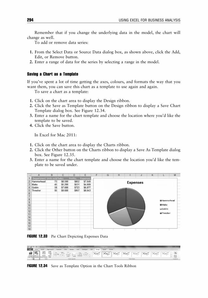
Remember that if you change the underlying data in the model, the chart willchange as well.

To add or remove data series:

1. From the Select Data or Source Data dialog box, as shown above, click the Add,Edit, or Remove button.

2. Enter a range of data for the series by selecting a range in the model.

Saving a Chart as a Template

If you’ve spent a lot of time getting the axes, colours, and formats the way that youwant them, you can save this chart as a template to use again and again.

To save a chart as a template:

1. Click on the chart area to display the Design ribbon.2. Click the Save as Template button on the Design ribbon to display a Save Chart

Template dialog box. See Figure 12.34.3. Enter a name for the chart template and choose the location where you’d like the

template to be saved.4. Click the Save button.

In Excel for Mac 2011:

1. Click on the chart area to display the Charts ribbon.2. Click the Other button on the Charts ribbon to display a Save As Template dialog

box. See Figure 12.35.3. Enter a name for the chart template and choose the location you’d like the tem-

plate to be saved under.

FIGURE 12.33 Pie Chart Depicting Expenses Data

FIGURE 12.34 Save as Template Option in the Chart Tools Ribbon

c12 22 June 2012; 19:5:45


4. Click the Save button. (See the Excel 2003 instructions available at www.wiley.com/go/steinfairhurst.)

To use the chart template:

1. Select a data range for the new chart.2. Click the dialog launcher, which is located at the lower-right of the Charts button

group. (Found in the Other menu in Excel for Mac 2011.)3. Select the template you’d like to use. See Figure 12.36.

Click on Set as Default Chart so that each time you create a chart, it will default toyour template. (Note that this function is unavailable in Excel for Mac 2011.) This isparticularly useful when using the F11 shortcut to create a chart.

HANDY CHARTING HINTS

Here are some handy charting hints:

n The formatting on most of the areas of the chart can be changed by double-clickingon the area you wish to change. You can play with this to make your graph lookmore attractive.

n The legend on the right-hand side can be resized, moved, or deleted by selecting it.n If the chart has been inserted in the worksheet, rather than on its own page, it can

be easily dragged around the worksheet or resized.

FIGURE 12.36 Using a Chart Template

FIGURE 12.35 Save as Template Option in the Chart Tools Ribbon

c12 22 June 2012; 19:5:45




n If you hide data in your source sheet, this will not show on the chart. Test this byhiding one of the columns on the Financials sheet and check that the month hasdisappeared on the chart. You can change the options under Select Data Source sothat it displays hidden cells. This is a new feature that was introduced in Excel2007, and it is unavailable in previous versions. See Figure 12.37.

n The chart can be changed to a different type of chart (e.g., a bar chart or a piechart) by right-clicking and selecting Change Chart Type.

n Including a data table (not to be confused with a sensitivity analysis data table) thatshows actual values below the chart is a great way to display the informationvisually while still providing detailed data. See Figure 12.38.

(See the Excel 2003 instructions available at www.wiley.com/go/steinfairhurst.)Select Show Data Table from the drop-down menu under the Data Table icon on theLayout tab (Format tab in Excel for Mac 2011) as shown in Figure 12.39.

FIGURE 12.37 Select Data Source Dialog Box

12000

Closing Cash

Café Cash versus Profit

Profit after Tax10000

8000

6000

4000

2000

�2000

0

Jan

1118.7 2345.3 526.4 1753.1 4950.7

1328.4 1309.5

3112.9 6607.6

1536.3 1120.5

9508.2 6096.3

326.67 326.67

7863 9575.6

288.87

6131.3

704.67�126.9 �51.33 �51.33 �580.5

Closing Cash

Profit after Tax

Feb Mar Apr May Jun Jul Aug Sep Oct Nov Dec

FIGURE 12.38 Line Chart with Data Table

c12 22 June 2012; 19:5:45



n Charts can be pasted directly into Microsoft Word or PowerPoint. Note that if yousimply copy and paste, the links to the underlying data in Excel will be maintained.This is fine, if you want to be able to edit the Excel data and have the chart update.Normally when you’ve copied and pasted a chart into Word or PowerPoint, youhave finished it and don’t want the chart to change at all. Therefore, it needs to bepasted as a picture. Copy the chart and then Paste Special, pasting the chart intothe destination document as a picture to make sure that the chart does not change.

TIP

To create a chart very quickly on a new sheet, highlight the data and use the F11shortcut. This automatically creates a column chart in all versions of Excel. In Win-dows versions you can change the default settings under Change Chart Type.

DYNAMIC RANGE NAMES

When creating a chart for which you are not sure of the size of the data, using dynamicnamed ranges can be particularly helpful.

The problem with specifying a range is that if someone adds data to right or belowthe table, it will not be included in the range. This can potentially cause error.

Let’s say that you have the data shown in Figure 12.40. You have defined a namedrange called Expense_data, which has a formula linking to it. Now, if a user wants toadd data to this table (e.g., another expense item in row 9, or another city in column J),this new data will not be included in the range.

FIGURE 12.39 Inserting a Data Table into a Chart

FIGURE 12.40 Source Data for Dynamic Named Range

c12 22 June 2012; 19:5:46


Let’s make this named range dynamic, so that if data is added to the table, it will beincluded in the range. Firstly, we need to work out how big the range is. We’ll do thisusing a COUNTA formula in row 1 and column A. This counts the number of cells thatare not blank.

Note that the data needs to be a block, with no blank rows or columns, as thiscould throw the formula off by a row or column.

Go to the Name Manager or and create a named range as shown in Figure 12.41.See “Named Ranges” in Chapter 5 for instructions on how to create a named range.

Instead of putting the absolute range of A1:I8 in the Refers To box, put the formula5OFFSET(A1,0,0,COUNTA(A:A),COUNTA(1:1)).

This is telling the named range to start at A1 and to go for as far up and down asthere is data. We are using the height and width sections of the OFFSET function in thiscase. For more detail on this function, see “OFFSET Function” in Chapter 6.

You can now refer to this named range in formulas, knowing that additional datawill always be captured within the range.

NOTE

It is not normally a good idea to use entire column or row references in formulas because they use a lotmore memory; however, using them in this case, there is no limitation on how large the range can grow.If memory is an issue, you may prefer to limit the range to 1,000 rows and columns, or as many as youthink your users may need. In this case you could add some colour markings so that user know whenthey have exceeded the range limits.

Using a Dynamic Range Name in a Chart

Dynamic named ranges are helpful when you are creating a chart with a variable numberof values. For example, let’s say you are creating a chart based on financial mode thatcontains a variable number of tenants. We know that users are unlikely to need to modelmore than five or 10 tenants in the model, but we’ve made the model flexible so thatusers can enter up to 25 tenants, just in case they need that many. If we set up the chartallowing for 25 tenants it would look perfectly ridiculous. See Figure 12.42.

FIGURE 12.41 Creating a Dynamic Named Range

c12 22 June 2012; 19:5:46


The chart looks much better if we only include the tenants that actually have datain the chart. See Figure 12.43.

However, using an ordinary chart, we’d need users to go into the source data andchange the chart range manually, which would be time-consuming and error-prone.The alternative is to create dynamic named ranges in the source data, and then refer tothe named ranges when creating the chart. This way the range (and therefore the labelspicked up in the chart) will automatically expand and contract, depending on whetherthe cells contain data or not. Unused tenancy cells will remain blank and will not beincluded in the chart.

NOTE

When using dynamic named ranges in a chart, each range must be one-dimensional (i.e., only containdata in a single row or column). You therefore need to create a range for the labels and then a separaterange for each series that appears on the chart.

2,500

2,000

1,500

500

Square Metres Rent

$0

$1,000

$2,000

$3,000

$4,000

$5,000

$6,000

$7,000

Tenan

t 1

Tenan

t 3

Tenan

t 5

Tenan

t 7

Tenan

t 9

Tenan

t 11

Tenan

t 13

Tenan

t 15

Tenan

t 17

Tenan

t 19

Tenan

t 21

Tenan

t 23

Tenan

t 25

�

1,000

Tenancy Rental Income vs Property Size

FIGURE 12.42 Chart with Variable Number of Tenants

Square Metres Rent

2,500

2,000

1,500

500

�

1,000

Tenancy Rental Income vs Property Size

Tenant 1 Tenant 2 Tenant 3 Tenant 4 Tenant 5$0

$1,000

$2,000

$3,000

$4,000

$5,000

$6,000

$7,000

FIGURE 12.43 Chart with Five Tenants

c12 22 June 2012; 19:5:46


CHARTING WITH TWO DIFFERENT AXES AND CHART TYPES

One of the best ways of analysing the output of your model is to plot two differentvariables on the same chart, so that we can understand trends and look for correlationsin the data. Sometimes the only way to spot a trend or an anomaly in the model is to lookat it graphically. For example, how does our overall revenue compare to head count?Surely as revenue increases so should head count, and if it doesn’t we need to understandwhy. What if we compare regions and their number of units sold and profit? Surely theregions with the highest number of units sold should be the most profitable? This maynot necessarily be the case. Let’s take a look at some data, and plot the number of unitssold and the profits using two different chart types on two axes.

If we have the data as shown in Figure 12.44, we can create a simple line chart. Theeasiest way to do this is to highlight the data in columns A, B, and D by holding downthe Control key.

Select the 2-D line from the Insert tab on the ribbon. In Excel for Mac 2011, selectthe 2-D line from the Chart tab on the ribbon. (See the Excel 2003 instructionsavailable at www.wiley.com/go/steinfairhurst.)

Note that you’ll need to hold down the Control key while selecting nonconsecutiveranges.

The chart will look something like Figure 12.45.The problem is that the chart looks quite nonsensical because we are plotting two

different types of units: number of units sold and profit (in dollars).The first thing we need to do is move the units sold to a new y-axis on the right-

hand side.

1. Select one of the series by clicking on it. Make sure the entire series has beenselected.

2. Right-click and go to Format Data Series.

FIGURE 12.44 Inserting a Line Chart

c12 22 June 2012; 19:5:46



3. On the Series Options tab, click on Secondary Axis instead of Primary Axis. SeeFigure 12.46.

4. This will create a new axis on the right-hand side. This can also be done on theLayout tab (or the Format tab in Excel for Mac 2011); simply click on FormatSelection, as shown in Figure 12.47.

Insert the axis labels to make your chart clearer.

FIGURE 12.46 Format Data Series, Secondary Axis

FIGURE 12.47 Format Selection (on the Layout Tab)

1200

1000

800

600

400

200

0Hammerhead Mako Goblin Thresher

Units sold

Profits

FIGURE 12.45 Preliminary Line Chart

c12 22 June 2012; 19:5:46


Choose Primary Vertical Axis Title and Secondary Vertical Axis Title from theAxis Titles on the Layout tab in the ribbon, as shown in Figure 12.48.

This will look better as a combination of a column and line graph, so let’s changethe Profit series to a column graph.

1. Select the Profit series.2. Right-click and select Change Series Type.3. Choose a column chart.

Your chart should look like Figure 12.49.Insert a title by selecting Chart Title from the Layout tab. (See the Excel 2003

instructions available at www.wiley.com/go/steinfairhurst.)

TIP

These charts can be a little confusing if you try to put too much in, so keep it simple bysticking to only two series. Make sure that the axes are formatted correctly if currencysymbols are appropriate. Leave the legend, which will make it clearer which section ofthe chart refers to which series.

BUBBLE CHARTS

Bubble charts are a variation of other types of graphs, combining elements from col-umn and scatter charts. They give the user a way to compare values based on therelative size of the bubble, as well as the location within the chart. They are most usefulwhen there are three data points to display.

FIGURE 12.48 Adding the Axes Titles in Excel 2007/10

c12 22 June 2012; 19:5:47



Let’s say you have collected the following historical information about yourcompany’s profits and profit margins by year:

Year Profit Number of Staff

2008 $50,000 232009 $35,000 172010 $40,000 202011 $18,000 92012 $60,000 302013 $45,000 22

Since you have three data points, it is difficult to represent this as a 2-D graph.Consider the following example of how the data could be charted. See Figure 12.50. Itcan be difficult to compare the relativity of the gross margin dollars and the grossmargin percentage. Essentially, having all of the information in this format loses theintended purpose.

In this situation, we can consider using a bubble chart. The same data presented ina bubble chart tells a different story. You are able to compare the profits and marginsby using the vertical rise of each bubble (profit) and its corresponding y-axis value,along with comparing the margins by looking at the size of the bubbles.

Creating a bubble chart is a bit more involved than a standard bar chart, but thefew extra steps are worthwhile.

$1,200 90

80

70

60

50

40

30

20

10

Ham

mer

head

Mak

o

Goblin

Thres

her

0

$1,000

$800

$600

$400

$200

$0

Prof

its

Uni

ts s

old

Profits Units sold

FIGURE 12.49 Completed Chart on Two Axes and Chart Types

c12 22 June 2012; 19:5:47


1. Open up a blank worksheet and start by entering the data as shown inFigure 12.51.

2. The columns are reflected on the bubble chart, as shown:a. The first column contains the values for the horizontal x-axis and it must

contain numerical data—text such as Area A, Area B, and so on will not showup on the x-axis.

b. The second column contains the values for the vertical y-axis.c. The third column will be shown as the size of the bubble.

3. The first trick with a bubble chart is that all data needs to be formatted asNumber; otherwise it will not be properly displayed. Change the formatting toensure the data has been formatted as a number.

4. We can now create a bubble chart from this data. The easiest way to do this isto highlight the whole range A2:C7, and create the chart. It is important toremember not to include the headers—another trick with bubble charts. Doing sowill cause errors.

5. Select the bubble chart under Other Charts from the column section on the Inserttab (or Charts tab in Excel for Mac 2011), and the basic bubble chart will appearautomatically. See Figure 12.52. (See the Excel 2003 instructions available at www.wiley.com/go/steinfairhurst.)

6. The chart should now look something like Figure 12.53 (although the coloursand background might look a little different, depending on which version ofExcel you are using).

FIGURE 12.51 Source Data

Profits and Number of Staff$70,000

$60,000

$50,000

$40,000

$30,000

$20,000

$10,000

$02008 2009 2010

23 17 20 9 30 22

2011 2012 2013

FIGURE 12.50 Data Shown in a Two-Dimensional Chart

c12 22 June 2012; 19:5:47




FIGURE 12.52 Inserting the Bubble Chart

$70,000

Series1$60,000

$50,000

$40,000

$30,000

$20,000

$10,000

$02007 2008 2009 2010 2011 2012 2013 2014

FIGURE 12.53 First Draft of Bubble Chart

c12 22 June 2012; 19:5:47


7. Click on the series legend and delete it.8. Add the title Profit & Staff. Click on the graph and select Chart Title from the

Layout tab. Right-click and go to Chart Options.9. Right-click on the bubbles to select them all, and choose Add Data Labels. The

default will be the sales amounts. To change this, right-click again on the bub-bles, and choose Format Data Labels.

Under LabelOptions, unselect y-axis, select Bubble Size, and also selectCenter.Your chart should be informed by the samples in Figures 12.54, 12.55, and 12.56.

Then, right-click on the actual labels, choose Format Data Labels, go toAlignment, and select Center under Label Position, and click OK.

FIGURE 12.54 Changing the Labels

FIGURE 12.55 Format Data Series Dialog Box

c12 22 June 2012; 19:5:47


10. To bold the data labels, you can highlight them first, then press Control þ B (thistrick works anywhere in Excel,Word, andmost programs). This is Command þ Bin Excel for Mac 2011.

11. Your bubble chart should look something like Figure 12.57.

WATERFALL CHARTS

Waterfall charts, also called bridge or stepped charts, have become popular in recentyears, particularly when displaying the output of a financial model. A waterfall chartdisplays very effectively the incremental impact of each period of time, or unit. It is atype of bar chart where the value of the second bar generally begins where the first onefinished. To illustrate, a waterfall chart might look something like Figure 12.58.

This kind of waterfall chart is very simple, and will only take a few minutes tobuild, as the incremental cash amounts for each month are always positive, and there

FIGURE 12.56 Format Data Labels Dialog Box

$0

$10,000

$20,000

$30,000

$40,000

$50,000

$60,000

$70,000

2007 2008 2009 2010 2011 2012 2013 2014

Profit & Staff

Prof

it

23

1720

9

30

22

FIGURE 12.57 Completed Bubble Chart

c12 22 June 2012; 19:5:48


are no values below the x-axis. First, we’ll take a look at creating this kind of verysimple waterfall chart, then we’ll tackle the more complex charts.

Creating a Basic Waterfall Chart (with Only Positive Values)

Let’s say you have a forecast for incoming cash for the next six months (see the data listthat follows).

Month Profit

Jan $250Feb $200Mar $1,000Apr $120May $650Jun $800

You could forecast it as a cumulative bar chart. See Figure 12.59.But we’d like to see the incremental contribution of each month individually,

which will add a new dimension to the analysis.Contrary to popular belief, you don’t need fancy software to build a basic waterfall

chart. They are really not that difficult to build in Excel and are achieved by a littletrick whereby we create a floating or dummy series in a stacked column chart.

1. Open a blank worksheet and start by entering the dates and your cash amount incolumns A and C as shown, leaving column B blank. See Figure 12.60.

2. In column B, we need to create a dummy series, which will be used to push eachcash series bar up to where the last one ended. So column B will contain thecumulative balance from the previous period. You’ll see what I mean in a minute.

3. We need to make cell B3 a cumulative balance, so the formula in cell B3 shouldbe ¼B21C2. Copy B3 down to B7. Let’s label it the Base column because it’seffectively where the bottom of each column starts. It should now look somethinglike Figure 12.61.

$0Jan Feb Mar Apr May Jun

$500

$1,000

$1,500

$2,000

$2,500

$3,000

$3,500Cash Forecast Waterfall

FIGURE 12.58 Completed Basic Waterfall Chart

c12 22 June 2012; 19:5:48


4. We can now create a stacked bar chart from this data. The easiest way to do thisis to highlight the whole range A2:C7, and create the chart.

5. Select the stacked column from the column section on the Insert tab (or theCharts tab in Excel for Mac 2011) and the chart will appear automatically. (Seethe Excel 2003 instructions available at www.wiley.com/go/steinfairhurst.)

The chart should now look something like this (although the colours andbackground might look a little different if you are using Excel 2003 or Excel forMac). See Figure 12.62.

FIGURE 12.61 Basic Waterfall Chart Formulas

FIGURE 12.60 Basic Waterfall Chart Workings Layout

Cumulative Cash Forecast$3,500

$3,000

$2,500

$2,000

$1,500

$1,000

$500

Jan Feb Mar Apr May Jun$0

FIGURE 12.59 Cumulative Cash Forecast Chart

c12 22 June 2012; 19:5:48



6. Click on the series legend and delete it.7. Add the title Cash Forecast Waterfall by clicking on the graph, and selecting

Chart Title from the Layout tab.8. Click on the bottom series and change the series fill colour of the bars to white or

no fill by right-clicking and selecting Format Data Series. You may also like toedit the colour of the chart series that is showing on the chart.

9. You can remove the background gridlines by clicking on them and deleting.10. If there is a border around the white series, you can remove this by going into

Format Data Series again and selecting the No Border option.11. Your waterfall chart should look something like Figure 12.63.

Creating a Waterfall Chart (with Positive and Negative Values)

What if your cash forecast changed, however, and in April you are expecting a poormonth, with a loss amount of $500? See the following list of data:

$3,500Cash Forecast Waterfall

$3,000

$2,500

$2,000

$1,500

$1,000

$500


FIGURE 12.63 Completed Basic Waterfall Chart

$3,500

$3,000

$2,500

$2,000

$1,500

$1,000

$500


CashBase

FIGURE 12.62 Draft Basic Waterfall Chart

c12 22 June 2012; 19:5:48


Month Profit

Jan $250Feb $200Mar $1,000Apr ($500)May $650Jun $800

Simply changing the data on your existing waterfall chart model will not displaythe chart correctly. Entering a negative value will cause the series to display below thex-axis, which is not correct. See Figure 12.64.

We’ll need to create separate columns for additional series in order to allow fornegative values in our waterfall chart.

1. Change the layout of your sheet so that it shows the negative and positive amountsin separate columns as shown below. Remove the dummy figures from column B.Even though the value in cell D5 is a negative amount, we will enter in it aspositive for the chart. See Figure 12.65.

2. Maintain a balance in row E. Cell E2 would be 5E11C2-D2. Copy this formuladown to E7 to achieve the following results. See Figure 12.66.

FIGURE 12.64 Incorrect Waterfall Chart (with Positive and Negative Values)

FIGURE 12.65 Waterfall Chart Workings Layout (with Positive and Negative Values)

c12 22 June 2012; 19:5:48


3. Now we’ll use the dummy column B as we did before, to control the steppingstones of our chart. The formula in cell B2 should be 5E1-D2. Copy it down therange. See Figure 12.67.

4. Generate a chart, as you did in the exercise above, for this data, excluding column E.See Figure 12.68.

5. Again, change the base series to white font or no fill.6. You may wish to show the negative cash amount in a different colour. If you’d like

to see all series the same colour, simply make them both the same.

FIGURE 12.67 Waterfall Chart Formulas (with Positive and Negative Values)

FIGURE 12.66 Waterfall Chart Formulas (with Positive and Negative Values)

FIGURE 12.68 Draft Waterfall Chart (with Positive and Negative Values)

c12 22 June 2012; 19:5:49


7. Practice changing the input numbers from positive to negative, and check that thechart is working correctly.

8. The final chart should look something like Figure 12.69.

Figure 12.69 is also useful for displaying the profitability of the company by cat-egory, instead of by time series.

In Figure 12.70, we have simply replaced the months with the revenue and expensecategories and changed the numbers. Using exactly the same simple template, we candisplay how much of the revenue is being spent in each expense category and howmuch residual profit is left.

Creating a Complex Waterfall Chart (with Positive and Negative ValuesCrossing the x-Axis)

You may have noticed that the charts we created above all remain as positive totalvalues. They will not work if the columns are below the x-axis. For example, if the cashloss amount (as shown in one of the last examples) was $2,000 instead of $500, thistemplate would not work correctly. See Figure 12.71.

FIGURE 12.70 Completed Profitability Waterfall Chart

Cash Forecast Waterfall

$2,000

$1,000

$1,500

$500


$2,500

$3,000

FIGURE 12.69 Correct Completed Waterfall Chart (with Positive and Negative Values)

c12 22 June 2012; 19:5:49


In order to create a waterfall chart that will handle both positive and negativevalues, as well as a balance that crosses the x-axis, we’ll need to create much morecomplex calculations. If you are sure that you don’t need this additional complexity,then one of the previous examples will suffice. However, if you spend the extra timesetting up the template as we will now discuss, the chart will work no matter what theparameters of the inputs are. Be warned: These formulas are not for the faint-hearted.You might prefer to simply type in the formulas as described above instead of trying tofollow the logic of what each formula is doing, as detailed in the following instructions.

1. To start, we need to treat the series separately depending on whether they arepositive or negative, and above or below the x-axis (or zero), so we need to plotfive series:a. Positive values above zero.b. Positive values below zero.c. Negative values below zero.d. Negative values above zero.e. The floating or dummy series (labelled blank in Figure 12.72).

2. Therefore you need to set up the sheet to look like Figure 12.72.3. Positive values above zero: To calculate this, we need to show the minimum of

the cumulative amount and the current month’s amount—but only if this value isgreater than zero. The formula in cell D2 should be 5MAX(0,MIN(SUM(B$2:B2),B2)). Copy it down the range.

FIGURE 12.72 Layout for Complex Waterfall Chart

FIGURE 12.71 Incorrect Waterfall Chart

c12 22 June 2012; 19:5:49


4. Positive values below zero: If the series goes below zero, we’ll need to know thedifference between the value entered, and the positive amount above zero (cal-culated in the last step), displayed as a negative amount. The formula in cell E2should be 5-MAX(0,B2-D2). Copy it down the range.

5. Negative values below zero:To calculate this, we need to show themaximum of thecumulative amount and the current month’s amount—but only if this value is lessthan zero. The formula in cell F2 should be 5MIN(0,MAX(SUM(B$2:B2),B2)).

6. Negative values above zero: If the negative values go above zero, we want tocalculate the difference between the value entered, and the negative amountabove zero (calculated in the last step). The formula in cell G2 should be ¼MAX(0,F2-B2). Copy it down the range.

7. The floating or dummy series: This calculation adds together both the highestand lowest of the cumulative values so that it can be a starting point for the otherseries. The formula in cell C3 should be 5MAX(0,MIN(SUM(B$2:B2),SUM(B$2:B3)))1MIN(0,MAX(SUM(B$2:B2),SUM(B$2:B3))). Copy it down therange. Note that cell C2 should be left blank.

8. Now that all five series have been completed, create the stacked chart byhighlighting the whole block except for the cash amounts in column B. Yoursheet should look something like Figure 12.73.

FIGURE 12.73 Draft Complex Waterfall Chart

$2,000

$1,000

�$1,000

$1,500

$500

�$500


Cash Forecast Waterfall

FIGURE 12.74 Completed Complex Waterfall Chart

c12 22 June 2012; 19:5:49


9. Change the colour of the blank series to white font or no fill.10. Now you have four different series in different colours. We want the positive and

negative amounts to be the same colour, so change them so that they are thesame. (You might prefer to have all four series the same colour.)

11. Delete the legend and add a title.12. Your waterfall chart should look something like Figure 12.74.

SUMMARY

Presenting the completed model is a part of the model-building process that is typicallynot done well by most financial modellers. The majority of the focus has been on thebuilding, structure, design, and layout, and on getting accurate calculations and results.

When senior managers or clients commission a financial model to be built, theyare less interested in the structure or calculations of the model than they are withthe output and the results of scenario analysis and sensitivity testing. Quite often themodeller does not consider how to best present and communicate these results to seniormanagers’ clients.

It’s important that at the end of the model-building process that the modeller spendssome time thinking about what the viewer of the model needs to see, whether it is a report,chart, or table, and how best to communicate both verbally and visually the methodology,assumptions, and results of the model in the clearest and most informative way.

c12 22 June 2012; 19:5:49


About the Author

Danielle Stein Fairhurst is the principal of Plum Solutions, a Sydney-based financialmodelling consultancy. With her talent for analytical modelling and professional

approach, Danielle helps her clients create meaningful financial models for businessanalysis. Over past decades she has worked in a number of industry sectors, includingtelecoms, information systems, manufacturing, and financial services, with solutionssuch as business cases, pricing models, and management reports. She is regularlyengaged as a speaker, facilitator, and consultant around Australia and globally.

She holds a master of business administration (MBA) from Macquarie GraduateSchool of Management, and has taught management accounting subjects at SydneyUniversity. Danielle lives in Sydney with her husband and two children, but travelswidely and enjoys the challenge of balancing a healthy family lifestyle with her passionfor financial modelling pedagogy.

babout 22 June 2012; 19:7:22

317

babout 22 June 2012; 19:7:22

About the Website

P lease visit this book’s companion website at www.wiley.com/go/steinfairhurst formore information on the tools discussed in this book. The website includes addi-

tional instructions, materials, downloads, and handy tips including:

n Instructions:n A detailed document containing instructions for how to use tools for which

instructions differ between versions—for those still using Excel 2003.n Materials:

n Excel Versions (Chapter 5).

n Additional Material:n Basic Formatting (Chapter 7).

n Break-Even Analysis (Chapter 9).

n How to Create a Basic Line Chart (Chapter 12).n Downloadable Resources:

n Online resources including a list of websites, blogs, and tutorials for Excel andfinancial modelling (Chapter 1).

n Shortcuts (Windows Version) (Chapter 5).

n Shortcuts (Mac Version) (Chapter 5).

n QA Log template (Chapter 10, Appendix 10.1).n Models:

n Model Assessment Checklist (Chapter 3).

n Salary Sacrifice Calculator (Chapter 7).

n Scenario Comparison (including both Exercise and Completed Versions)(Chapter 11).

n Waterfall Chart (including both Exercise and Completed Versions)(Chapter 12).

. . . and much more.

both 22 June 2012; 19:22:45

319


both 22 June 2012; 19:22:46

Index

Absolute referencing, 87, 94�95ActiveX controls, 170�171Add-ins, 6�10, 19, 199�200Aggregation functions, 64�65, 187Alignment, 133, 258, 272, 306Amortisation schedule, 127, 130Ampersand, 49Analysis ToolPak, 9AND, 83�84Area chart, 281, 287, 290Array formulas, 179�180, 182,

239, 256Assumptions documentation, 5, 27, 32, 39, 42,

45�46, 48, 52, 57, 154Assumptions layout, 21Audit tool, 9AVERAGEIFS, 99�100AVERAGE, 80�81, 84, 92Axes, 246, 288, 294, 300�303

Balanced scorecard, 5Bar chart, 139, 278�280, 286, 290, 303,

307�309Benchmarking, 5Best practice, ix�x, 3, 5�6, 15, 17, 23,

32�34, 39, 40�43, 45, 47, 49, 52,57, 60�62, 86, 90, 92, 107, 109, 180,209, 216, 235, 245, 251

Binary code, 169Boolean logic, 169Break-even analysis, 229�230Break-even point, 232Bubble chart, 282, 289,

302�305, 307Budgeting & Forecasting in Excel

(course), ixBulletproofing, 254Business case, 2, 13, 24, 42, 48, 57, 121, 210,

252, 276

Cell link, 164, 166, 168, 268�269Cell referencing, 41, 86�89, 92, 100, 219,

227, 247�248, 266

Charts, x, 4�5, 8, 25�26, 28�29, 31, 33,143�144, 157, 228, 246, 275�279,282�283, 285�291, 294�295, 297, 302,304, 307�309, 313

Chart type, 145, 279, 282, 288Checkboxes, 146, 164CHOOSE, 112, 113, 269Circular reference, 67�70, 197Colour coding, 26, 41, 171Colour scales, 141, 260Column chart, 282�283, 285�287, 297Combo box drop-down, 254, 268, 269, 273Communication, 14, 15, 17Compounding, 73, 127, 201�209Conditional formatting, 4, 28, 65, 133,

139�143, 188, 260�263Control key, 175Cost of capital, 13, 48, 121�123, 126,

213�214, 216COUNT, 76, 79, 81COUNTIF, 65, 72, 93�95, 97�98, 100COUNTIFS, 93, 97�98, 100Cover sheet, 14, 24�26, 36CSE formulas, 182Currency symbols, 136, 302Custom formatting, 120, 133, 135, 137

Dashboard, 2, 5, 288Data bars, 139Data collection, 31Data tables, 27, 180, 239, 256, 260, 272�273Data validation, 44, 153, 154, 254, 266, 268,

269, 273Data validation drop-down, 254Data validation input messages, 44Dates, 25, 46, 112�113, 115�119, 121,

135�136, 204�205, 308DAY, 118�119DB, 221, 223�224DDB, 221, 224Debt, 69, 122, 126�127, 214�216, 255Declining balance value methods, 222Depreciation methods, 220�222

bindex 22 June 2012; 19:14:35

321

Design skills, 14, 19, 21Developer tab, 158�159, 190�191Discount rate, 216Double declining balance method, 224Drop-down boxes, 25, 27, 30, 90, 157, 254,

266, 270

EFFECT, 127, 206�208Effective rates, 206�208Enter key, 54�55, 243EOMONTH, 9, 116�117, 227Equity, 122, 214�216Error checks, 25, 54, 63, 65, 70, 96Excel versions, 30, 135Excel 2003, 8�9, 30, 43�44, 46�47, 59,

67�68, 70, 92, 97�99, 127, 133, 139,149�150, 151, 154, 158, 178�179, 184,186�187, 189, 192, 195�196, 236, 237,243, 255, 258, 263, 272, 295�296, 302,304, 309

Excel 2007, 7�9, 44, 60, 70, 73�74, 97, 120,125, 127, 139�141, 143, 152, 155,157�158, 170, 187, 191, 195�196, 198,203, 208, 237�238, 263, 293, 302

Excel 2010, 68, 133, 135, 140�143, 152,157�158, 190

Exponential operations, 204

F9, 76, 78, 83, 229, 242File structure, 36�37, 151Filter, 41, 97, 117, 187, 197Financial functions, 72, 121Fixed declining balance method, 223Fixed interest rate, 130, 201Flag, 236Font, 14, 26, 36, 40, 46, 73, 133, 137, 139, 169,

194, 211, 260, 264, 267, 275, 312, 316Footnoting, 45, 47, 52Form control, 157�159, 167, 169, 170�171,

196, 254, 268Format control, 166, 168Formatting, x, 3�4, 14, 25, 27�28, 41, 46,

50�51, 65, 75, 77, 119�120, 133�143,146, 171, 178, 188, 193�195, 231, 248,259�263, 271, 277, 295, 304

Formatting:basic, 133custom, 50, 138

Formula, 1, 3�4, 9�11, 16�18, 21, 23,26�27, 32�34, 36, 40�41, 47, 49�52,54�57, 59�79, 82, 83, 84�116, 118,121, 123�133, 139, 148, 150, 152, 153,

157, 169, 170, 173, 178�184, 188,197�198, 200�205, 207�212,215�219, 221�231, 235�244,246�248, 256�258, 261�271,297�298, 308�309, 311�312,314�315

Formula errors, 9, 54Function, x, 7, 9�11, 14, 16�17, 21, 30�32,

37, 49�52, 63�66, 71�86, 92�131,133�134, 137, 143, 158, 160, 169�171,173, 182�187, 190�191, 198�203,205�208, 211, 216, 218�219, 221�227,233, 239, 248, 251, 255, 257�258, 262,266, 268�269, 279, 295, 298

Funding, 69, 252�253FVSCHEDULE, 203

Golden rules, 22Grouping, 137, 147, 173, 178�179, 200Growth, 4, 21, 42, 48, 53, 60, 73, 201�207,

214�215, 247

Hiding, 142, 147, 173�175, 177�178,200, 296

HLOOKUP, 72, 103�107, 211�212Hurdle rate, 121Hyperlinks, 43, 46�48, 52

Icon sets, 140�141, 143IF, 16, 40, 63�66, 71�72, 82�86, 111, 169,

205, 211, 217, 268IFERROR, 66�67In-cell comments, 43�44, 154Indexation, 56, 201, 206, 248, 253Inflation, 25, 40, 53, 201, 205�206, 207Information requests, 35Inherited model, 235Input sheet, 25, 26Interest, 1, 3�4, 7, 18, 53, 68�69, 72, 116,

121�131, 143, 184�185, 190, 201,203�204, 206�209, 215, 230, 252�253,255�273, 275, 293, 316

Interest calculations, 116Interest calculations:circular reference 67, 68, 69, 70, 197

IPMT, 129�131IRR, 13�14, 71�72, 121�126, 213, 216ISERROR, 66Iterative calculations, 69

Key assumptions, 14, 25, 39, 42, 57, 276KPI, 5

bindex 22 June 2012; 19:14:36

322 INDEX

Labelling, 41, 247Line chart, 228, 230, 277�280, 286�288,

290�291, 296, 300�301Linked text, 49, 52Linking, 2, 5, 32, 36�37, 39�41, 49, 52,

60�63, 70, 90, 97, 106�107, 157, 183,209, 236, 251, 265, 297

Linking:to external files, 61, 70

Loan calculations, 126, 206�207Loan rates, 207Logic, 2, 12�13, 15�17, 19, 21, 24�26,

28, 31�34, 37, 51�52, 56�57, 72,76, 79, 82�83, 117, 125, 161�162,169, 199, 236, 239, 243, 245�249,273, 314

Logic errors, 33�34, 56�57Logical functions, 72, 82LOOKUP, 86, 100, 104�107, 211�212,

217�219Lookup functions, 100, 107, 218

Macro, 11, 16, 30�31, 35, 41, 69, 90, 158,167, 173, 176�177, 187, 189�195,197�198, 200, 270

Macro:buttons 195

Management report, 3, 9, 187Manual sensitivity analysis, 265MAX, 72, 76, 79�80Methodology, 19, 52, 57�59, 91, 265, 273,

276, 316MIN, 76, 79�80, 82Mixed referencing, 41, 88Model audit, 55, 245Model layout 16, 22, 31MONTH, 118�119

Named ranges, 9, 32, 61, 62, 89, 91�92, 106,109, 157, 298�299

Nested formulas, 85NOMINAL, 127, 206�209, 247Nominal rates, 127, 208NOW(), 113, 115, 133�134NPV, 24, 48, 72, 121�123, 125�126,

213�214, 216, 276Number formats, 136Numeracy, 15, 19

OFFSET, 109�111, 236, 298Option button, 157, 162�164

OR, 84Oral presentation 275

Payback period, 121, 210, 212�213Period, 24, 42, 69, 121�123, 125�130,

201�202, 204, 207�213, 220�221,223�226, 278, 307�308

Pie chart, 279, 281, 287�288, 290, 292,294, 296

Pivot tables, 41, 95, 97, 173, 186�188PMT, 72, 127�131, 184�185,

257�258, 262PPMT, 129�131Pricing, 2, 12�13, 22, 25, 36�37, 56�57, 61,

85�86, 105�106, 197, 215�217, 228,233, 245

Pricing model, 12�13, 22, 36, 215Principal, 126�131, 201, 203Profit, 2, 4, 13, 16, 24, 50�51, 68�69, 123,

139, 184, 197, 211�212, 220, 227�231,233, 247, 261, 265, 267, 272, 276�277,282, 288�289, 296, 300�304, 306�308,311, 313

Progressive tiering table, 218Project evaluation, 121, 213Project planning, 4, 8, 37Protection, 34, 147�150, 154, 177�178,

244, 247Purpose of model, 250

QA (Quality Assurance), 33�36, 245�250QA log, 246, 248�250

Radar chart, 289Radio button, 162Rate, 1, 2�10, 13�16, 18, 21�27, 31�35, 37,

39, 42, 48, 50�55, 57, 58, 61, 63, 69�70,73, 78�79, 84, 88, 92, 103, 116,121�130, 136�137, 146, 157, 178,182, 184�185, 201�210, 213�228,230�231, 239, 245�249, 252�253,255�262, 264�265, 288, 299, 307,311�312, 314, 316

Redundant assumptions, 235Relative referencing, 88Remove duplicates, 187Repayments, 121, 126�129, 131, 184, 257Ribbon, 68, 119, 133, 144�146, 152�153,

158�161, 163, 165, 168, 190�196,199, 236�237, 241�243, 291, 294�295,300, 302

bindex 22 June 2012; 19:14:36

Index 323

Scenarios, 2, 3, 27, 29, 36, 56, 82, 182, 233,246, 251�257, 260�261, 265�266, 268,270, 272�273, 275�276

Scenario Manager, 254�256Scenario methods, 254, 264, 273Security settings, 190, 192, 198Sensitivity analysis, x, 3, 40, 56, 122, 180,

182, 209�210, 246, 251�253, 256�257,261, 265, 273, 275

Sensitivity testing, 276, 316Shortcuts, 66, 74�77, 92, 239SLN, 221�222, 226�227Solver, 8, 9Sparklines, 143�147, 289Spin button, 25, 165Spreadsheet, 1� 4, 7, 9�10, 14, 17, 19, 30, 48,

53, 55�56, 62, 91, 134, 139, 148, 178,196, 199�200, 203, 235, 244�247,255�256

Stress-testing, 34, 56, 246, 251�253, 257, 273SUM, 71, 76, 78, 84, 182, 212SUMIFS, 9, 93, 95, 97�100, 187SYD, 221, 225

Tax, 12, 25, 48, 56, 72, 79, 82, 85, 112,117, 128�129, 197, 208, 215�216,218�220, 227

Tiering table, x, 86, 102, 216, 218Time series, 23�24, 313TODAY(), 113, 115, 134Tool selection, x, 53Tracing dependents, 237

Trace error, 239Training course, 17, 19, 190TRANSPOSE Array Function, 183TRIM, 102�103

User-friendly (features), 24, 30�31, 51,166, 180

Variance analysis, 2, 16, 139VBA, 9, 167, 176, 189, 190, 194�195,

198, 268Visual Basic Editor 176, 177VLOOKUP, 11, 66�67, 71�72, 86,

100�107, 118, 153, 182, 212, 217�219,266, 268

Waterfall, 307�316WEEKDAY, 113, 117�118, 121Weighted average cost of capital (WACC), 25,

122, 213�216What-if analysis, 184, 252, 255

XIRR, 125�126XNPV, 125�126

YEAR, 117�118

#DIV/0! 34, 66#NAME? 239#N/A 66, 102#REF! 111, 236, 275

bindex 22 June 2012; 19:14:36

324 INDEX

Using excel for business analysis

Business

Transcript of Using excel for business analysis