Bowling Green State University

From the SelectedWorks of Sheryl L. Coombs

May 15, 2009

Using Computational Fluid Dynamics toCalculate the Stimulus to the Lateral Line of aFish in Still WaterMark A. RapoHoushuo JiangMark A. GrosenbaughSheryl L. Coombs, Bowling Green State University

Available at: https://works.bepress.com/sheryl_coombs/3/

1494

INTRODUCTIONAll fishes possess a mechanosensory lateral line system, whichresponds to the surrounding water motion relative to the fish’s skin.Such water motion can be generated due to a variety of biotic andabiotic events, including encounters with prey, predators,conspecifics and inanimate obstacles. Consequently, the lateral linesystem plays an important role in mediating fish behavior indifferent ecological contexts. Over the years, there is a rich bodyof literature documenting various aspects of lateral line function,ranging from biomechanical and neural principles of operation tobehavioral significance (for reviews, see Dijkgraaf 1963; Kalmijn,1988; Denton and Gray, 1988; Coombs et al., 1988; Coombs et al.,1992; Bleckmann, 1993; Montgomery et al., 1995; Schellart andWubbels, 1997; Coombs and Montgomery, 1999; Bleckmann et al.,2001; Janssen, 2004; Mogdans, 2005; van Netten, 2006; Bleckmann,2008).

The lateral line system consists of superficial (SN) and canal (CN)neuromast subsystems, which are morphologically, physiologicallyand functionally different (e.g. Coombs et al., 1988; Münz, 1989).In terms of the basic structure, both types of neuromasts consist ofmechanosensory hair cells covered by a gelatinous cupula. However,SNs are generally smaller in diameter (≤100μm) than CNs (up toseveral thousands of microns) and contain fewer hair cells (<~100)compared with CNs (~200–10,000) (Münz, 1989). Although therelative numbers and spatial distribution of SNs versus CNs overthe head and body are quite species-specific, most if not all fish

species (e.g. the mottled sculpin Cottus bairdi) have both types ofneuromasts (Coombs et al., 1988). A reported exception is theplainfin midshipman fish, Porichthys notatus, whose trunk lateralline only has SNs (Weeg and Bass, 2002). The clear distinctionbetween SNs and CNs is that SNs are located superficially on theskin surface whereas CNs reside just below the skin surface in afluid-filled canal that opens up to the surrounding water via a seriesof pores – one pore between each pair of neuromasts. Thus, whereasSN cupulae protrude directly into the water surrounding the fish,CN cupulae protrude into the canal fluids. Hair cells of both typesare mechanically excited by viscous coupling with the surroundingfluid motion via the overlying cupula. An SN cupula, protrudinginto the surrounding water, responds to the local fluid velocity field.A CN cupula, being inside the canal, responds to the fluid motioninduced by the local net acceleration of the water against the fishskin, which is also proportional to the pressure gradient across thesurrounding two canal pores (Denton and Gray, 1983; Kalmijn,1989). Physiologically, SNs and CNs are likely to be innervated bydifferent afferent fibers (Münz, 1985). Thus, fish have separatechannels for measuring the velocity and acceleration fields producedby not only periodic (Denton and Gray, 1983; Münz, 1985; Coombsand Janssen, 1989; Coombs and Janssen, 1990; Kroese and Schellart,1992) but any stimuli (Bleckmann, 2008).

Attention has been paid to the relative contributions of SNs andCNs to the orienting behavior of fish in response to both live andartificial prey (e.g. a chemically inert vibrating sphere). For the

The Journal of Experimental Biology 212, 1494-1505Published by The Company of Biologists 2009doi:10.1242/jeb.026732

Using computational fluid dynamics to calculate the stimulus to the lateral line of afish in still water

Mark A. Rapo1, Houshuo Jiang1,*, Mark A. Grosenbaugh1 and Sheryl Coombs2

1Department of Applied Ocean Physics and Engineering, Woods Hole Oceanographic Institution, Woods Hole, MA 02543, USA and2Department of Biological Sciences and J. P. Scott Center for Neuroscience, Mind and Behavior, Bowling Green State University,

Bowling Green, OH 43402, USA*Author for correspondence (e-mail: hsjiang@whoi.edu)

Accepted 29 December 2008

SUMMARYThis paper presents the first computational fluid dynamics (CFD) simulations of viscous flow due to a small sphere vibrating neara fish, a configuration that is frequently used for experiments on dipole source localization by the lateral line. Both two-dimensional (2-D) and three-dimensional (3-D) meshes were constructed, reproducing a previously published account of a mottledsculpin approaching an artificial prey. Both the fish-body geometry and the sphere vibration were explicitly included in thesimulations. For comparison purposes, calculations using potential flow theory (PFT) of a 3-D dipole without a fish body beingpresent were also performed. Comparisons between the 2-D and 3-D CFD simulations showed that the 2-D calculations did notaccurately represent the 3-D flow and therefore did not produce realistic results. The 3-D CFD simulations showed that thepresence of the fish body perturbed the dipole source pressure field near the fish body, an effect that was obviously absent in thePFT calculations of the dipole alone. In spite of this discrepancy, the pressure-gradient patterns to the lateral line systemcalculated from 3-D CFD simulations and PFT were similar. Conversely, the velocity field, which acted on the superficialneuromasts (SNs), was altered by the oscillatory boundary layer that formed at the fish’s skin due to the flow produced by thevibrating sphere (accounted for in CFD but not PFT). An analytical solution of an oscillatory boundary layer above a flat plate,which was validated with CFD, was used to represent the flow near the fish’s skin and to calculate the detection thresholds of theSNs in terms of flow velocity and strain rate. These calculations show that the boundary layer effects can be important, especiallywhen the height of the cupula is less than the oscillatory boundary layer’s Stokes viscous length scale.

Key words: computational fluid dynamics, fish, lateral line system, dipole source, oscillatory boundary layer.

THE JOURNAL OF EXPERIMENTAL BIOLOGY

1495CFD of lateral line stimulus

mottled sculpin, both neurophysiological and controlled behavioralstudies suggest that the acceleration-responsive CNs, rather thanthe velocity-responsive SNs, mediate the orienting behavior (e.g.Coombs and Janssen, 1990; Coombs et al., 2001). However, sculpinlarvae can feed in the dark on free-swimming Artemia at distancewith the aid of SNs (Jones and Janssen, 1992). Despite the fact thatthe SNs of the sculpin larvae are eventually embedded into the canalto become CNs, the prey detection at the larval stage is due tomovement of the SN cupulae in response to local flow velocities.Similar results were also found for the larvae of the willow shinerGnathopogon elongatus caerulescens for whom it was shown thatthe number of Artemia consumed per larva was proportional to thecupular length and saturated at lengths above ~100μm (Mukai etal., 1994). Later, Mukai performed a controlled experiment usingwillow shiner larvae that demonstrated the role of mechanoreceptionby the SNs on prey detection (Mukai, 2006). Abdel-Latif et al.showed that, under still water conditions, the blind cave fishAstyanax mexicanus could still detect and approach a small vibratingsphere, presumably by means of its SN subsystem after thedestruction of its CN subsystem (Abdel-Latif et al., 1990). However,there is a debate (e.g. Coombs et al., 2001; Mogdans, 2005)concerning the exact detection mechanism, as the pressure fieldaround a dipole source could theoretically be detected by thepressure-sensitive ear of this species.

The stimulus to the lateral line system is the relative motionbetween fish skin and adjacent water, which is described by thespatio–temporal varying flow velocity and pressure fieldssurrounding the lateral line system. In general, such flow velocityand pressure fields are not (fully) measured in neurophysiologicaland behavioral studies – particularly in regions close to the skinwhere boundary layers are important. The inability to measure andspecify the stimulus hinders our understanding of the lateral linesystem (Coombs and Montgomery, 1999). Potential flow theory(PFT) has been used in the past to address this issue. For example,the potential dipole source flow equations were used to model thepressure field due to a vibrating sphere near a fish body (e.g. Coombset al., 1996; Coombs and Conley, 1997a; Coombs and Conley,1997b; Conley and Coombs, 1998; Coombs et al., 2000; Curcic-Blake and van Netten, 2006). The same equations were used tocalculate the slip flow velocity along the fish skin, caused by a nearbyvibrating sphere (e.g. Kroese et al., 1978). (In PFT, the boundarycondition at a solid wall requires only that the fluid velocity normalto the wall be equal to the wall velocity. Thus, the fluid is allowedto ‘slip’ past the wall surface in the wall tangential direction.) Thisslip flow velocity was taken as the stimulus to the SNs, with theassumption that the cupular lengths were long enough to penetratethe viscous boundary layer along the fish’s skin. More sophisticatedpotential flow solutions have been developed to calculate the slipflow velocity distribution (and pressure distribution) over idealizedfish body geometry (Hassan, 1985; Hassan, 1992a; Hassan, 1992b;Hassan, 1993). All of these studies ignore the fact that the real flowhas to satisfy the no-slip boundary condition at the fish skin due toviscosity, i.e. zero relative velocity at the skin in both the normaland tangential directions [see pp. 140–143 in Panton (Panton, 1996)].

Computational fluid dynamics (CFD) solves the Navier–Stokesequations, which include the viscous terms. CFD simulations havebeen previously employed to investigate tadpole swimming (Liu etal., 1996; Liu et al., 1997), fish undulatory swimming (Carling etal., 1998; Kern and Koumoutsakos, 2006; Borazjani andSotiropoulos, 2008), dorsal–tail fin interaction in swimming fish(Akhtar et al., 2007), oral cavity flow in ram suspension-feedingfish (Cheer et al., 2001), jet flow behind a modeled swimming squid

(Jiang and Grosenbaugh, 2006) and drag forces acting on a simulatedneuromast inside a fish lateral line trunk canal with the canal flowdriven by a two-dimensional (2-D) vortex street outside the canal(Barbier and Humphrey, 2008). To our knowledge, no previous CFDsimulations have studied the flow due to a vibrating sphere (i.e. adipole source) or a swimming prey-like object near a three-dimensional (3-D) fish body and calculated directly the stimuli tothe lateral line system. CFD is useful because it has the ability toconsider realistic fish body geometry and realistic spatialarrangements of the fish body and the signal source and because itcan simultaneously output both the pressure and flow velocity fieldsat the lateral line locations. In the present study, we carried out aCFD numerical investigation of the flow due to a vibrating spherenear a mottled sculpin in still water. We performed a series ofsimulations of a prey-tracking sequence of a mottled sculpin as itresponded to an artificial prey (i.e. vibrating sphere). Theapproximate shape and orientation of the fish body were takendirectly from a video recording of a real tracking sequence (Coombsand Conley, 1997a). The series of simulations show explicitly howthe presence of the fish body perturbs the contour lines of constantpressure of the dipole field.

The flow due to the vibrating sphere must satisfy the no-slipboundary condition at the fish’s skin. This produces an oscillatoryboundary layer of sheared flow that affects the magnitude of thehydrodynamic signals detectable by the SNs. As important as thiseffect is, we were not able to simulate it directly for a 3-D fish-shapedbody because of limited computational resources. Instead, we usedCFD to calculate the 3-D oscillatory boundary layer flow along a flatplate produced by a nearby vibrating sphere. We then used this resultto validate an analytical model of an oscillatory boundary layer flow.The analytical model was then applied to a number of previousneurophysiological and behavioral experiments to calculate detectionthresholds that take into account viscous effects.

This paper considers only flow due to the motion of the vibratingsphere in calm water. A future paper will include the added effectsof an ambient, unidirectional current.

MATERIALS AND METHODSSimulations of flow around a sculpin due to a nearby

vibrating sphereOur computational domain and meshes for the fish simulations wereconstructed according to the experimental designs of Coombs andConley (Coombs and Conley, 1997a; Coombs and Conley, 1997b)and by using the geometry and mesh generation software, GAMBIT(Lebanon, New Hampshire, USA). The geometry consisted of amottled sculpin-like body, sitting on a solid flat bottom and a nearby3 mm-radius solid sphere executing a vibration. The sphereperformed sinusoidal motions along an axis for a series of burstsof 500ms on and 500ms off so as to dismiss the effects of acousticstreaming, which took more than 500ms to develop. The sculpinbody was constructed to approximately match the dimensions ofthe real fish. The length of the main body of the fish was 8cm, witha portion of the tail extending an additional 1cm. The body was2cm in width at its thickest point, which is just in front of the pectoralfins. The dorsal fin extended about 0.5cm above the fish in its frontand about 1cm above in its rear. The pectoral fins and tail fin were0.5mm thick whereas the dorsal fin was 1mm thick. Both a 2-Dsetup and a 3-D setup were considered. The purpose was tocompare the 2-D results with the 3-D results and to find out if the2-D setup was accurate enough to reproduce the involved fluidphysics. (The 2-D assumption is often adopted in studies but it isnecessary to check its validity before use.)

THE JOURNAL OF EXPERIMENTAL BIOLOGY

1496

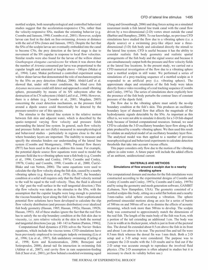
In the 2-D setup (Fig.1), the cross-sections of the sculpin bodyand of the sphere formed the inner boundaries of a rectangularcomputational domain (275�100cm). The sculpin body was heldstationary. The cross-section of the sphere was given a prescribedaxis of motion along with a solid-body vibration with the followingtime history:

u(t) = U0cos(ωt) , (1)

where U0 is velocity amplitude of the sphere vibration, t is time andω=2πf where f is the vibration frequency in Hz. A no-slip boundarycondition was prescribed at the sculpin body and at the perimeterof the sphere cross-section. Also prescribed was a zero pressureinlet boundary condition at the outer boundaries of the domain (toapproximate an infinite domain). The area between the inner andthe outer boundaries of the domain was discretized into triangularmeshes. The consecutive nodal points on the sculpin cross-sectionwere 2mm apart, close to the spacing between two consecutivelateral line CNs in the trunk canal of a real sculpin (Coombs et al.,1988). The perimeter of the sphere cross-section was equallydivided by 20 nodal points. The size of the triangular meshes wasincreased gradually from the inner boundaries to the outer boundariesof the domain. A dynamic mesh model was used to representexplicitly the vibrating motion of the sphere cross-section, i.e. themeshes surrounding the sphere cross-section deform as the spherecross-section moves (Fig.1B).

In the 3-D setup (Fig.2), a box-shaped computational domain(60�40�10cm) was considered. The surface of the 3-D sculpinbody was discretized into triangular meshes with 2mm edge lengths.The sphere surface was divided into triangular meshes with 1mmedge lengths. The volume between the sculpin body surface, thesphere surface and the surface of the box-shaped computationaldomain was discretized into tetrahedral control volumes. Adeforming mesh zone was placed around the sphere surface toaccommodate the sphere motion. Suitable boundary conditions wereprescribed similar to those in the 2-D setup.

In the present still-water case, flow was generated exclusivelyfrom the vibration of the sphere. The flow was assumed laminar,incompressible and Newtonian and was governed by the unsteadyincompressible Navier–Stokes equations together with the continuityequation. Throughout this study, the fluid density, ρ, was1.0�103 kg m–3 and the fluid kinematic viscosity, ν, was1.0�10–6 m2 s–1. The governing equations with the above-describedcomputational domains and simulation setups were solved by acommercially available, finite-volume code, FLUENTTM (v. 6.2.16,Lebanon, New Hampshire, USA). The third-order MUSCL(Monotone Upstream-Centered Schemes for Conservation Laws)scheme was used for spatial interpolation. The PRESTO! (PREssureSTaggering Option) scheme was selected as the discretizationmethod for pressure. The PISO (Pressure-Implicit with Splitting ofOperators) scheme was used for pressure–velocity coupling.Temporal discretization was a first-order implicit scheme. Adynamic mesh model built into FLUENTTM was employed toexplicitly consider the sphere vibration.

To examine the effect that the fish body and fins have on thereceived dipole pressure signal, two body geometries wereconsidered: body with fins extended (Figs1 and 2) and body withfins retracted (this geometry is not shown). Also considered was avirtual-body case where the standard potential dipole source flowsolutions (Pozrikidis, 1997) in an unbounded domain (without anyinternal fish boundaries) were evaluated at virtual lateral linelocations identical to those on a real fish body. For all cases, thetime step for integration was set at 1/100th of the vibration period.

M. A. Rapo and others

The 2-D flow field was initialized by simulating 200 time steps;the 3-D flow field was initialized by simulating 1000 time steps.This was done to allow transients to decay. After the initial start-up, flow velocity and pressure fields were saved at each time stepfor post-processing.

For the 2-D setup, pressure gradients were calculated along thesculpin cross-section by:

where p1 and p2 are pressure values at two consecutive nodal pointson the profile, which were 2 mm apart by mesh construction and

dp

ds=

p2

− p1

2 , (2)

B

275 cm

100

cm

A

Deforming zone

Static zone

Zoom

p2 p1

dpds

=p2 − p1

2C

Source side lateral line nodes

Back side lateral line nodes

Front side lateral line nodes

Fig. 1. (A) 2-D computational domain for a circular cylinder (with cross-section identical to that of the sphere) vibrating nearby a sculpin cross-section. (B) A zoomed-in view of the meshes surrounding the cylinder andthe sculpin. The vibrating motion of the cylinder was represented by asmall rectangular deforming mesh zone that surrounds the immediate areaof the cylinder. (C) Node locations around the sculpin cross-section wherepressures at pore openings were evaluated. The convention for calculatingthe pressure difference is identified by the direction of the arrows. Thepressure at the arrow tip (p1) is subtracted from the pressure at the arrowtail (p2). The distance between two consecutive pore openings is assumedto be 2 mm. dp/ds denotes the pressure gradient along the profile.

THE JOURNAL OF EXPERIMENTAL BIOLOGY

1497CFD of lateral line stimulus

dp/ds denotes the pressure gradient along the profile. The orderingof p1 and p2 was defined by the arrows shown in Fig. 1C. For the3-D setup, nodal points (Fig. 2C) were manually selected toapproximately follow what might be considered the true locationsof lateral line canals on the mottled sculpin [see fig. 1 in Coombs(Coombs, 2001)]. As the selected nodal locations were not evenlyspaced, a spline curve for the pressure values was fitted to thoselocations for each of the lateral line sections (i.e. trunk canals,infraorbital canals, supraorbital canals, mandibular canals andoccipital canal) (Fig. 2C). Next, pressure values were sampledevery 2mm on each fitted curve and then used in Eqn2 to calculatepressure gradients. Also, for comparison purposes, the mid-planecross-section of the 3-D fish body was identified, and pressuregradients were calculated along the mid-plane cross-section profile(Fig. 2D), similar to what was done for the 2-D setup.

To validate the 3-D setup and simulation procedure, a few casesof a vibrating sphere above a flat plane wall were simulated. Themesh densities over the sphere surface and over the plane wall werethe same as those used for the 3-D simulations that incorporatedthe fish body. The numerical results for the magnitudes of thepressure and pressure gradient (which are not affected by viscosity)showed excellent agreement with the PFT solution of a spherevibrating above a plane wall (Fig.3). The 2-D setup and simulationprocedures were validated in a similar way (Rapo, 2009).

Flat-plate oscillatory boundary layer simulations andanalytical model

3-D simulations were also performed of the formation of oscillatoryboundary layers due to the vibration of the sphere. When a spherevibrates near a stationary fish body in otherwise quiescent water,two oscillatory boundary layers will form, one on the sphere andone on the fish skin. Outside these two boundary layers, PFT isapplicable (Fig.3). The significance of the boundary layer on thesphere was recognized by Kalmijn (Kalmijn, 1988). A mathematicalformulation was provided by van Netten (van Netten, 2006).

Both oscillatory boundary layers have the same Stokes viscouslength scale, δ, defined as:

where ν is the kinematic viscosity of the fluid and ω=2πf. (Forf=50Hz, which is a typical condition used in many experiments,δ~80μm.) Because of the oscillatory nature of the motionconsidered, viscous diffusion due to the presence of the wall cannotpenetrate beyond a distance of order δ away from the wall [e.g. pp.263–272 in Panton (Panton, 1996)]. The magnitude of the velocityof the oscillatory boundary layer of the fish skin is usually muchweaker than that of the oscillatory boundary layer surrounding thesphere, with the difference in magnitude depending on the distancebetween the sphere and the fish’s skin.

The 3-D computational mesh as described in the previous sectionwas unable to resolve the oscillatory boundary layer along a fish-shaped body because the distances from centroids of the wall-adjacent control volumes to the fish skin were ~290μm, which ismuch larger than δ. To resolve this boundary layer, we would needto use a much finer near-wall mesh, which our current computationalsetup could not handle. To deal with this problem, we used CFDto calculate, instead, the flow along a flat plate produced by a nearbyvibrating sphere. Anderson et al. (Anderson et al., 2001) have shownthat flat-plate boundary layer theory can be used to model theboundary layer along a fish, and we adopted this assumption forthe oscillatory case. The flat-plate geometry required fewer mesh

δ =2νω

, (3)

10 c

m

60 cm

40 cm

Zoom

p2 p1

dpds

=p

2− p

1

2

A

B

C

Back side Source side

Front side

p1 p2

dpds

=p

2− p

1

2

D

Trunk canals

Source side nodesBack side nodesFront side nodes

Infraorbital canals

Supraorbital canals

Mandibular canals

Occipital canal

Fig. 2. (A) 3-D computational domain for a sphere vibrating nearby a sculpinbody. (B) A zoomed-in view of the surface meshes of the sphere and of thesculpin, with nodes spaced approximately 1 mm apart on the sphere and2 mm apart on the sculpin. The vibrating motion of the sphere was directlyrepresented by a deforming mesh that surrounds the immediate vicinity ofthe sphere and is contained inside a small rectangular prism (not shown).(C) Node locations around the sculpin body where pressures wereevaluated, including those points which fall directly on the sculpin’s lateralline system (marked by various colors). (D) Points around the sculpin mid-plane cross-section, where pressures were interpolated from the pressuredata computed on the 3-D sculpin surface. In both C and D, the conventionfor calculating the pressure difference is identified by the arrow direction.The pressure at the arrow tip (p1) is subtracted from the pressure at thearrow tail (p2). The distance between two consecutive pore openings isassumed to be 2 mm. dp/ds denotes the pressure gradient along theprofile.

THE JOURNAL OF EXPERIMENTAL BIOLOGY

1498

points overall than a fish-shaped body while still allowing for a finegrid-point spacing at the wall (grid-point locations were at 0, 5, 13,24, 39, 61μm … away from the wall). The plane wall surface wascovered by quadrilateral meshes. A deforming mesh zone, consistingof tetrahedral meshes, was present around the sphere so as torepresent the motion explicitly. The volume between the deformingmesh zone and the boundary layer mesh zone close to the planewall was divided into tetrahedral control volumes. The samenumerical schemes and time step as previously described were used.Large parameter ranges as found in the literature were considered;velocity amplitude 7 mm s–1≤U0≤314 mm s–1, sphere radius2.5 mm≤a≤18 mm and distance from sphere to fish body1.1cm≤r≤20cm.

For the remainder of this section, we consider a sphere withvibration axis parallel to the wall. We define a Cartesiancoordinate system such that the positive x-direction is parallel tothe wall and to the axis of the sphere vibration, the positive y-direction is the wall-normal direction toward the sphere, thepositive z-direction is chosen such that the defined xyz-coordinatesystem satisfies the right-hand rule and u, v and w are the x-, y-and z-velocity components, respectively. Using this Cartesiancoordinate system, the strain rate tensor, S, can be defined as (e.g.Pozrikidis, 1997):

Also we define the overall strain rate (S) as:

S is a useful measure of the magnitude of fluid-parcel deformationirrespective of directional information. Within the oscillatoryboundary layer at the fish’s skin, bending of an SN cupula will beaffected by the dynamic behavior of S surrounding the cupula aswell as the whole velocity profile, u(y,t).

We use the CFD simulation of the oscillatory flat-plate boundarylayer to validate a simpler analytical model, which we then use inthe next section of this paper to analyze threshold velocity and Sresponses of SNs. The following is the analytical model. For a spherevibrating parallel to a flat plane wall with r>>δ, the wall-parallelvelocity profile along the wall-normal (y-) direction has anapproximate solution:

This solution is for the flow created due to an oscillating plate, whichis written in the frame of reference of the plate (e.g. Pozrikidis, 1997).The boundary-layer edge velocity is replaced by the wall slip flowvelocity that corresponds to a potential dipole source placed at the

u y, t( ) = C a, δ( ) U0a

r

⎛⎝⎜

⎞⎠⎟

3

e− y /δ cos ω t + φ − y / δ( ) − cos ω t + φ( )⎡⎣ ⎤⎦ . (6)

S =

2∂u

∂x

⎛⎝⎜

⎞⎠⎟

2

+ 2∂v

∂y

⎛⎝⎜

⎞⎠⎟

2

+ 2∂w

∂z

⎛⎝⎜

⎞⎠⎟

2

+∂u

∂y+

∂v

∂x

⎛⎝⎜

⎞⎠⎟

2

+∂u

∂z+

∂w

∂x

⎛⎝⎜

⎞⎠⎟

2

+∂v

∂z+

∂w

∂y

⎛⎝⎜

⎞⎠⎟

2 . (5)

S =

∂u

∂x

1

2

∂u

∂y+

∂v

∂x

⎛⎝⎜

⎞⎠⎟

1

2

∂u

∂z+

∂w

∂x

⎛⎝⎜

⎞⎠⎟

1

2

∂u

∂y+

∂v

∂x

⎛⎝⎜

⎞⎠⎟

∂v

∂y

1

2

∂v

∂z+

∂w

∂y

⎛⎝⎜

⎞⎠⎟

1

2

∂u

∂z+

∂w

∂x

⎛⎝⎜

⎞⎠⎟

1

2

∂v

∂z+

∂w

∂y

⎛⎝⎜

⎞⎠⎟

∂w

∂z

⎛

⎝

⎜⎜⎜⎜⎜⎜⎜⎜

⎞

⎠

⎟⎟⎟⎟⎟⎟⎟⎟

. (4)

M. A. Rapo and others

center of the sphere and an image dipole source placed an equaldistance below the wall to satisfy the potential flow ‘zero-normal-flow’ wall boundary condition. C(a,δ) is the amplitude correction termdue to the sphere boundary layer and φ is the phase delay. Both arecalculated according to van Netten (van Netten, 2006) as:

Because this case involves only unidirectional flow, S is just |du/dy|,which is found by taking the y-derivative of the velocity profile(Eqn 6):

The velocity and strain rate profiles calculated using Eqns 6–8 arein excellent agreement with the results of CFD simulations fordifferent parameter values (Fig.4).

The maximum strain rate at the wall, Swall, is found by settingy=0 and taking the maximum, which occurs at (ωt+φ)=3π/4. Thisgives:

The maximum shear stress at the wall is just μSwall, where μ is thefluid dynamic viscosity, which is equal to 1.0�10–3 kgm–1 s–1. Eqn9 is a useful measure of the forces acting to displace the cupula,especially when the height of the cupula, H, is unknown. If the heightis known, another useful measure is maximum average strain rate,Saverage, along the cupula, which is defined as:

where Δu is the maximum velocity difference between the cupulartip and base over the whole vibration cycle.

RESULTSSimulated prey-tracking sequence: the 2-D case

The initial three steps of a six-step, prey-tracking sequence recordedby Coombs and Conley (Coombs and Conley, 1997a) for a mottledsculpin were simulated using the 2-D setup (Fig.5A) and the 3-Dsetup (Fig.5B–D). The sphere had a radius of 3mm, oscillating ata frequency of 50Hz with source velocity amplitude of 0.18ms–1

(peak-to-peak). These three positions were selected because theyrepresented different relative locations between the fish’s body (andpectoral fins) and the dipole source. In the starting location at thetime of signal onset (Position No. 1, Fig.5A,B), the sphere wasslightly less than a body length away and was closer to the fish’stail than head. In the second position (Position No. 2, Fig.5C), thesphere was also less than a body length away and was lateral to thepoint of pectoral fin insertion. In the third position (Position No. 3,Fig.5D), the dipole source was in a more frontal location much closerto the head of the fish than the tail.

For 2-D CFD simulations, with the fish body present (columns2 and 3 in Fig.5A), the iso-pressure lines terminate on the fish bodyand are more concentrated around curved regions of the body andsharp edges of the fins. These local concentrations of pressure

Saverage =Δu

H , (10)

Swall = 2 C a, δ( ) U0

δ

a

r

⎛⎝⎜

⎞⎠⎟

3

. (9)

d u y, t( )dy

= C a, δ( ) U0

δa

r

⎛⎝⎜

⎞⎠⎟

3

e− y /δ sin ω t + φ − y / δ( ) − cos ω t + φ − y / δ( ) . (8)

C = C12 + C2

2 φ = arctan C2 / C1( )C1 = 1+

3δ2a

C2 =3δ2a

1+δa

⎛⎝⎜

⎞⎠⎟

. (7)

THE JOURNAL OF EXPERIMENTAL BIOLOGY

1499CFD of lateral line stimulus

contours cannot be predicted from PFT without the fish body present(column 4 in Fig.5A). When the fins are extended (column 2 inFig.5A), a zone of near constant pressure is created on the side ofthe fish closest to the source (the ipsilateral side) in a small, localizedpocket behind the extended fin and side of the body. The presenceof the fish body shields a large region of water from the dipolesource, creating a region of near constant pressure along thecontralateral side of the fish opposite the dipole source.Consequently, the pressure gradient seen by the lateral line on boththe ipsi- and contralateral side tends toward zero as the fin insertionpoint (indicated by the red arrow in column 2 in Fig.5A) isapproached. This is in contrast to the case with a streamlined bodypresent, where only the body curvature itself determines how thepressure field is affected (column 3 in Fig.5A). In this case, thereis no constant pressure region on the ipsilateral side of the fish nearthe pectoral fin. The iso-pressure lines of the hydrodynamic field

without a body present are obviously undisturbed (column 4 inFig.5A).

Simulated prey-tracking sequence: the 3-D caseThe same sculpin tracking sequence was simulated using the 3-Dsetup (Fig.5B–D). The presence of the fish body perturbs thepressure field but to a lesser extent than for the 2-D case. Whereasthere are clear differences between the results for fins extended andfins retracted in the 2-D case (columns 2 and 3 in Fig.5A), there isno such detectable difference in the 3-D case (columns 2 and 3 inFig.5B). The reason is that, in the 3-D case, the dipole source flowfield extends over and under the fins, as well as around them andtherefore there is no longer any zone of near constant pressure behindthe extended fins. In the 3-D case, the presence of the fish bodystill shields a region of water on the contralateral side from the dipolesource but the overall effect of this shadow zone is weaker than for

–20–15

–10

–5

0

5

10

15

20

–5

0

5

10

15

20

01

2

3

4

5

6

7

8

–10 –8 –6 –4 –2 0 2 4 6 8 10 –10 –8 –6 –4 –2 0 2 4 6 8 10

–10 –8 –6 –4 –2 0 2 4 6 8 10

–3

–2

–1

0

1

2

3

–10 –8 –6 –4 –2 0 2 4 6 8 10

Distance (sphere diameters)

Sphere height

ZY

X

ZY

X

2

–2

0

–1

1

� 10–2

Sphere oscillating parallel to wall Sphere oscillating perpendicular to wall

Wall

pρωaU0

p2

p1

p2

p1

A B

C D

E F

� 10–2� 10–2

� 10–3

pρωaU0

� 10–3dp/dsρωU0

1.8 diam – PFT3.5 diam – PFT8.5 diam – PFTNumerical sim

Fig. 3. Comparison between the 3-D computational fluid dynamics (CFD) simulations (symbols in C–F) and the potential flow theory (PFT) (solid lines inC–F) for a sphere vibrating above an infinite flat plane wall. The PFT solution consists of a dipole source above the wall and an image dipole source belowthe wall to satisfy the zero-normal-flow wall boundary condition. The axis of sphere vibration is either parallel (left column) or perpendicular (right column) tothe wall. Iso-pressure contours of the instantaneous pressure field are depicted in (A) and (B). Line plots of the instantaneous pressure (C,D) and pressuregradient (E,F) along the wall are shown for three distances (1.8, 3.5 and 8.5 sphere diameters) between the sphere and the wall. U0, velocity amplitude ofthe sphere vibration; ρ, fluid density; ω=2πf; p1, p2, pressure values along the wall, which are used to calculate the pressure gradients, dp/ds.

THE JOURNAL OF EXPERIMENTAL BIOLOGY

1500 M. A. Rapo and others

the 2-D case. The overall pressure field calculated from PFT withoutthe fish body present is different from that obtained from the 3-DCFD simulations but the magnitude of the calculated pressuregradients along the virtual fish mid-plane profile are quite similarto those calculated from the 3-D CFD simulations. This is not thecase in the 2-D simulation.

The magnitude of the pressure gradient around the fish body isdirectly related to the location of the dipole source. Spatial variationsare most striking when comparing the ipsilateral side of the fishclosest with the dipole source and the contralateral side. However,equally noticeable are the differences in magnitude seen betweenthe head and trunk of the fish. In the starting position (Fig.5B), themagnitude of the pressure gradient is larger on the ipsilateral sidenear the end of the trunk (blue line) than at the front of the fish(green line). In the second position (Fig.5C), the magnitude of thepressure gradient is similar for both the head and trunk (green lineversus blue and red lines) but a clear difference still exists betweenthe two sides of the fish (blue line versus red line). In the thirdposition (Fig.5D), the head of the fish is much closer to the dipolesource, while the tail is further away. The pressure gradientamplitude has more than quadrupled for the front sections of thehead canals (green line). Also, the contrast in pressure gradientsbetween the two sides of the fish has widened (blue line versus redline).

Fig.6 shows the pressure gradients along the lateral line canalsof the mottled sculpin (Fig.2C) based on the 3-D CFD results forthe third position of the video sequence (Fig.5D). Interestingly, theipsilateral (positive numbers on the horizontal axis) pressure-gradient patterns along supraorbital, infraorbital and mandibularcanals with different elevations (above and below the eye and alongthe lower jaw) but largely overlapping azimuths (rostro-caudalextents) tend to converge on the same, nearly redundant pattern.However, patterns on the ipsi- and contralateral side (negativenumbers) are dramatically different. Ipsilateral patterns have steeperslopes and distinct zero-crossings (locations where the direction orsign of the pressure gradient changes from positive to negative). Inthis case, the true source location is near the zero-crossing point onthe ipsilateral side.

Applying the oscillatory boundary layer solution to realexperiments

We applied the analytical solutions Eqns 6 and 9 for the oscillatoryboundary layer to the results of a number of previousneurophysiological and behavioral experiments designed to measurethe threshold sensitivity of SNs in different species and under varyingconditions. We used the reported experimental parameters to re-compute values of the velocity threshold at the tip of the SN cupula

–1 –0.5 00

1

2

3

4

5

6

7

0 0.5 10

1

2

3

4

5

6

7

CFD,S

U / δ

Analytic solution,|du/dy |

U / δ

y/δ –1 –0.5 0

0

1

2

3

4

5

6

7

0 0.5 10

1

2

3

4

5

6

7

or

A

B

C

D

Analytic solution, u /UCFD, u /U

–1 0.5 00

1

2

3

4

5

6

7

0 0.5 10

1

2

3

4

5

6

7

–1 0.5 00

1

2

3

4

5

6

7

0 0.5 10

1

2

3

4

5

6

7

�

� �

�

u /U� |du/dy |

U / δ�

S

U / δ�

Fig. 4. Comparison between the 3-D computational fluid dynamics (CFD)simulations (symbols) and the analytical solution (solid lines from Eqns6–8) for the oscillatory boundary layer at the surface of an infinite flat planewall, created by a sphere vibrating above and parallel to the wall. Vertical(y-) profiles are compared at the wall location directly below the equilibriumposition of the sphere. The left column corresponds to the along-wall flowvelocity, u, and the right column corresponds to the strain rate, S, and theshear rate, du/dy. A variety of sphere-to-wall distances (r), source vibrationmagnitudes (U0), frequencies (f), and sphere radii (a) are considered. Fourexamples are shown here: (A) f=30 Hz, r=10a, U0=0.04 m s–1, phaseωt=0.4π, where ω=2πf and t the time. (B) f=45 Hz, r=20a, U0=0.1 m s–1,phase ωt=1.6π. (C) f=50 Hz, r=3.67a, U0=0.007 m s–1, phase ωt=2π.(D) f=75 Hz, r=40a, U0=0.03 m s–1, phase ωt=2π. δ, Stokes viscous lengthscale; U�, fluid velocity just outside the oscillatory boundary layer.

THE JOURNAL OF EXPERIMENTAL BIOLOGY

1501CFD of lateral line stimulus

and the strain rate threshold at the wall, Swall. The parameters neededfor the analysis are a, r, f, U0 and H. The following is a descriptionof the different experiments used in the analysis and the results ofthe calculations.

Kroese et al. (Kroese et al., 1978) used a=1.55mm oscillating atf=20Hz parallel to the skin and perpendicular to the longitudinalaxis of an SN of the clawed frog (Xenopus laevis), withU0=5�10–4 ms–1 and placed at a distance of r=3.75mm from theskin. They assumed an SN cupula height of 100μm and found avelocity threshold of 38μms–1 based on the potential flow equations.The Stokes viscous length scale for these particular experimentalconditions calculated using Eqn3 is δ=126μm. Thus, the cupulawould be fully immersed in the oscillatory boundary layer flow.From Eqn6, we find that u at the tip of the cupula after beingcorrected for the boundary layer effects is 30μms–1 (about 21%smaller than Kroese et al.’s threshold estimated from PFT). FromEqn9, we find that the maximum Swall threshold is 0.45s–1 and fromEqn10 the maximum Saverage is 0.30s–1.

Coombs and Janssen estimated velocity thresholds for SNslocated along the trunk lateral line of mottled sculpin fromneurophysiological measurements (Coombs and Janssen, 1990). Thevelocity field was produced by an oscillating sphere whose centerwas placed r=15mm away from the fish trunk. The radius of thesphere was 3mm and it was oscillated in a direction perpendicularto the substrate (up/down with respect to the fish) at frequencies inthe range 10–500Hz. The source velocity amplitude of the spherecorresponding to the threshold response, while not explicitly given,can be calculated using the dipole equations (e.g. Pozrikidis, 1997)and the results given in fig.7 of Coombs and Janssen (Coombs andJanssen, 1990). We estimated that the peak-to-peak accelerationthreshold (at the fish) for SNs at 10Hz is –55dB re. 1ms–1 and thatthe threshold acceleration increases linearly by about 7.5dBoctave–1.From this, we determined that the corresponding source velocityamplitude of the sphere needed to produce the measured peak-to-peak acceleration in an unbounded fluid to be about 3.5mms–1 for10 Hz, 5.3 mm s–1 for 50 Hz and 6.3 mm s–1 for 100 Hz. Thecorresponding velocity amplitude threshold at the tip of the SNcupula based on potential flow equations (with values doubled toaccount for the presence of the fish body) is 28μms–1 at 10Hz,42μms–1 at 50Hz and 50μms–1 at 100Hz. The velocity thresholdvalues corrected for the oscillatory boundary layer effects (assumingH=100μm) are 18μms–1 at 10Hz, 42μms–1 at 50Hz and 54μms–1

at 100Hz, where δ=176μm at 10Hz, δ=80μm at 50Hz and δ=56μmat 100Hz. The velocity threshold for the 10Hz case is lower thanthe potential flow case due to the slowing of the flow near the wall,the velocity threshold for the 50Hz case is unchanged and thevelocity threshold for 100Hz case is actually slightly higher thanthe potential flow case due to overshoot in the velocity profile(Fig.7). {At certain distances from the wall the phase lag in viscousstresses is so great that the viscous and pressure terms actually addtogether. The combination of these forces accelerates the fluid toproduce the overshoot [pp. 268–269 in Panton (Panton, 1996)].}The experimental parameter values give maximum Swall of 0.24s–1

at 10Hz, 0.78s–1 at 50Hz and 1.30s–1 at 100Hz. With H=100μm,the maximum Saverage are 0.18s–1 at 10Hz, 0.42s–1 at 50Hz and0.54s–1 at 100Hz.

Coombs et al. used a vibrating sphere to stimulate CNs andSNs and to see which subsystem was responsible for the orientingresponse in mottled sculpin (Coombs et al., 2001). When theydisabled SNs, the fish was still able to orient towards the vibratingsphere. However, when they disabled CNs, response rates fell tospontaneous levels, indicating that the SNs were not used for

orienting. An alternative explanation is that during the experiment,the stimulus to the SN was below its threshold velocity and strainrate. In their experiments, Coombs et al. used a sphere of radiusof 3 mm placed 3–6 cm from the fish (Coombs et al., 2001). Thesource velocity was 5.5 cm s–1 for the 10 Hz signal and 9.0 cm s–1

for the 50Hz signal. The maximum velocity at the tip of the cupula[taking viscous effects into account and assuming that H is100μm, as in Coombs and Janssen (Coombs and Janssen, 1990)]is 5–36μm s–1 for 10 Hz (range of values in all cases depend onthe distance between the sphere and the fish) and is 11–89μm s–1

for 50 Hz. The maximum Swall was 0.06–0.47 s–1 for 10 Hz and0.21–1.66 s–1 for 50 Hz. With H=100μm, the maximum Saverage

are 0.05–0.36 s–1 for 10 Hz and 0.11–0.89 s–1 for 50 Hz. Thesevalues are above the SN threshold values measured by Coombsand Janssen (Coombs and Janssen, 1990) when the fish was 3 cmfrom the sphere but are below threshold values when the fish was6 cm from the sphere.

Alternately, Abdel-Latif et al. showed that blind cave fish couldorient toward a vibrating sphere even when the CN subsystem wasdisabled, indicating that the fish were relying on the SN subsystemto locate the sphere (Abdel-Latif et al., 1990). Their experimentalparameters were a=2.5mm, r=20cm, f=10–90Hz and displacementamplitudes = 0.2–1.4 mm. A positive behavioral response forfrequencies 50Hz and 70Hz was reported for all amplitudes. Thecorresponding velocity thresholds (taking into account the oscillatoryboundary layer effects) based on an SN height of 200μm (Teyke,1988) are 0.14–0.96μms–1 at 50Hz and 0.19–1.31μms–1 at 70Hz(depending on the displacement amplitude). These values are wellbelow the threshold values of the SNs of other species describedabove. In addition, the maximum Swall range is 0.0023–0.016s–1 at50Hz and 0.0037–0.026s–1 at 70Hz, and the maximum Saverage rangeis 0.0007–0.048s–1 at 50Hz and 0.0010–0.0065s–1 at 70Hz. Againthese are extremely low values, even acknowledging the possibilityof signal startup transients, which from the present numericalsimulation briefly increased the maximum wall strain rate up to 4times the steady state value.

DISCUSSIONThe results from the 2-D and 3-D simulations are significantlydifferent. Qualitatively, the perturbation to the dipole pressure fielddue to the presence of fish body is much more prominent in the2-D CFD results than in the 3-D CFD results. Similarly, the effectof the pectoral fin is also more visible in the 2-D than in the 3-Dresults. For our specific case, the 2-D and 3-D CFD simulationsproduced the ‘Mexican-hat’ shaped pressure-gradient patterns withtwo zero-crossings for the head canal (green line of column 2 inFig. 5D for 3-D, not shown for 2-D). However, the simulationsproduced completely different pressure-gradient patterns for thetrunk canals (Fig. 5A versus 5B). Quantitatively, the mostprominent difference is that the 2-D pressure-gradient magnitudesare 20 times larger than those calculated using the 3-D geometry.Taken together, this raises concerns about using 2-D results tocalculate the hydrodynamic stimulus, at least for the presentsituation of a fish using its lateral line system to locate a vibratingsphere.

The 3-D results confirm that it is valid to use PFT to predict thespatial patterns of pressure gradient that affect the canal subsystem.The CFD simulations show that the fish body does perturb the dipolepressure field but only to a small extent, such that the pressuregradients evaluated along the lateral line locations are quite similarto those calculated from the 3-D virtual body case using PFT. Thisconfirms the effectiveness of using PFT to estimate pressure-gradient

THE JOURNAL OF EXPERIMENTAL BIOLOGY

1502 M. A. Rapo and others

Fig. 5. See next page for legend.

THE JOURNAL OF EXPERIMENTAL BIOLOGY

1503CFD of lateral line stimulus

patterns to the canal subsystem created by a vibrating sphere in stillwater (Goulet et al., 2008). The 3-D CFD results do show that theextended fins significantly distort the dipole pressure field locally.The fact that the lateral line trunk canals of the mottled sculpin arerouted above the pectoral fins is probably of morphologicalsignificance, as it appears that this may limit the distortion in thereceived signal.

Our higher resolved CFD boundary layer simulations using a flat-plate model highlight the fact that a vibrating sphere generates anoscillatory boundary layer at the fish’s skin. The resulting flowvelocity signal to the SNs and their responses are greatly affectedby characteristics of the oscillatory boundary layer, which includeits thickness (characterized by the Stokes viscous length scale) andthe time-varying and height-varying flow magnitude and direction.Because of the presence of a boundary layer at the fish’s skin, thevelocity and velocity gradient patterns that act on the SNs cannotbe predicted by PFT. In particular, there is a phase difference(Fig.4A) between the flow velocity outside and inside the oscillatoryboundary layer. Also, there is overshooting of the flow velocityinside the boundary layer (Fig.4C,D), such that the velocity insidethe boundary layer can be greater than the outside flow. Thus, theheight of the cupula becomes an important parameter. For example,a cupula with a shorter height that is completely immersed in the

boundary layer will experience a weaker integrated flow over itslength than a taller cupula that extends outside the boundary layer.Consequently, a weaker response from the shorter cupula will beexpected. Mukai et al. found that the feeding rate of the willowshiner larvae consuming Artemia was proportional to the cupularlength on the larva body and saturated at lengths above ~100μm(Mukai et al., 1994). The trend of their fig.1 curve relating thefeeding rate to the cupular length corresponds well with the trendof the curves shown in Fig.7 of the present study, which can beinterpreted as the maximum tip-to-base velocity difference as afunction of neuromast height for three different frequencies. Fig.7may provide an explanation to their results, provided that the larvaeuse the SNs to detect appendage-beating movement of Atemia.

There is a minimum cupular displacement that must occur in orderfor the neuromast to respond, corresponding to a minimum velocitywhose drag force causes the displacement. This is called thevelocity threshold. Although the velocity threshold may be species-specific, the CNs probably respond to internal canal fluid velocitiesas low as 1–10μms–1 (van Netten, 2006). Inside the subdermal canal,the velocity is driven by the pressure difference between poreopenings, which translates to an acceleration threshold of0.1–1mms–2 (van Netten, 2006). The SNs respond to as little as25–60μms–1 (for a review, see van Netten, 2006). These resultswere obtained using PFT with the assumption that the cupular heightis larger than the boundary layer thickness. Using our analyticaltreatment, we showed that the oscillatory boundary layer formed atthe fish’s skin should be taken into account when estimating thesevelocity thresholds. The oscillatory boundary layer correction canbe significant depending on the cupular height relative to theboundary layer thickness. Re-analysis of Coombs and Janssen(Coombs and Janssen, 1990) gives a threshold velocity range of18–54μms–1 over a frequency range of 10–100Hz, when theoscillatory boundary layer effects are taken into account. Thevelocity threshold can also be defined as the maximum tip-to-basevelocity difference experienced by the cupula, because the basevelocity is zero. This is species-specific and depends on a numberof parameters, including cupular height and shape, as well as internalcupula stiffness (McHenry et al., 2008).

From CFD outputs, one may calculate maximum wall-strain rates,which are a measure of the near-wall fluid-parcel deformationprobably experienced by the SNs and are independent of cupularheight. For the mottled sculpin of the Coombs et al. (Coombs et al.,2001) experiment, the maximum wall strain rates given in theprevious section corresponded to the threshold values of SNs (eitherjust above or just below, depending on the starting distance of thefish from the vibrating dipole source). At the same time, theacceleration experienced by the lateral line canal subsystem (basedon Fig.6) is 5–50mms–2, which is many times stronger than thereported acceleration detection thresholds of CNs. This is consistent

–1 –0.8 –0.6 –0.4 –0.2 0 0.2 0.4 0.6 0.8 1

–0.8–0.6–0.4–0.2

00.20.40.60.8

1� 10– 3

Location along lateral line (BL)

Tail TailContralateral Front Ipsilateral

–1

dp/d

s

ρωU

0

Trunk canals

Infraorbital canals

Supraorbital canals

Mandibular canals

Occipital canal

Fig. 6. The complete dipole source pressure-gradient signalto the whole canal lateral line system, calculated from 3-Dcomputational fluid dynamics (CFD) and evaluated for strikeposition No. 3 as shown in Fig. 5D. U0, velocity amplitude; ρ,fluid density; ω=2πf; dp/ds, pressure gradient.

Fig. 5. Comparison between 2-D calculations (A) and 3-D calculations (B),and comparison between 3-D computational fluid dynamics (CFD)(columns 2 and 3 in B–D) and 3-D potential flow theory (PFT, column 4 inB–D) results when the pectoral fins are either included (column 2) orexcluded (columns 3 and 4). The calculations correspond to a video-recorded sequence of a mottled sculpin’s step-by-step approach towardsan artificial prey – in this case a sinusoidally vibrating sphere [fromCoombs and Conley (Coombs and Conley, 1997a)]. The first three steps ofthe prey-tracking sequence are illustrated, including the initial orientingresponse at signal onset (A and B are for the same step) followed by twosubsequent approach steps (C,D). Each block in columns 2–4 contains aplot of the iso-pressure contours of the normalized instantaneous pressurefield that surrounds the sculpin and the vibrating sphere. Plotted in thelower panel are distributions of normalized pressure gradient along thethree major portions of the lateral line canal system: the trunk canal on theipsilateral (I) side of the body with respect to the dipole source (blue curve),the trunk canal on the contralateral (C) side of the body (red curve) and thefrontal canals (F) on the head (green curve). T stands for the tail position.The pressure contours in column 4 correspond to the solution of a 3-D (2-Din A) dipole source in an unbounded fluid, unperturbed by the presence ofthe fish. The pressure gradient values plotted in column 4 are calculatedfrom the unperturbed pressure field but the magnitudes are doubled toaccount for the potential flow wall-boundary condition of the fish and tofacilitate comparison with the CFD solutions. The red arrow in column 2 ofA indicates the pressure gradient results for the pectoral fin insertionpoints. U0, velocity amplitude; ρ, fluid density; ω=2πf; a, sphere radius;dp/ds, pressure gradient; p, pressure.

THE JOURNAL OF EXPERIMENTAL BIOLOGY

1504 M. A. Rapo and others

with the conclusion that the acceleration-responsive CNs, rather thanthe velocity-responsive SNs, mediate the mottled sculpin’s orientingbehavior to the vibrating sphere (e.g. Coombs et al., 2001). However,all the SN thresholds calculated for the blind cave fish of the Abdel-Latif et al. (Abdel-Latif et al., 1990) experiment are extremely lowas compared with those numbers obtained for other experiments.This raises concerns regarding claims that the SNs were used fordetecting the dipole source, especially since these otophysan fishhave pressure-sensitive ears that could have easily detected thepressure changes of a nearby dipole source of the same frequency(Montgomery et al., 2001).

LIST OF ABBREVIATIONSa sphere radiusC, C1, C2 amplitude correction termCFD computational fluid dynamicsCN canal neuromastdp/ds pressure gradientdu/dy shear ratee mathematical constant ef vibration frequencyH cupula heightp1, p2 pressure values at two consecutive nodal points on the profilePFT potential flow theoryr distance from the sphere to the fish bodyS strain rate tensorS strain rateSaverage average strain rateSN superficial neuromastSwall wall strain ratet timeu x velocity componentu(y,t) velocity profileU0 velocity amplitude of the sphere vibrationU� fluid velocity just outside the oscillatory boundary layerv y velocity componentw z velocity componentδ Stokes viscous length scaleΔu maximum velocity difference between cupular tip and baseμ fluid dynamic viscosityν fluid kinematic viscosity

ρ fluid densityφ phase delayω 2πf2-D two-dimensional3-D three-dimensional

The authors are grateful to the Woods Hole Oceanographic Institution AcademicPrograms Office for graduate research support provided to M.A.R. The authorsgratefully acknowledge NSF for support of this research under grants IOS-0718506 to H.J. and IBN-0114148 to M.A.G. The authors are grateful to twoanonymous reviewers, who provided insightful comments that improved the finalpaper. The authors thank A. H. Techet for helpful discussions.

REFERENCESAbdel-Latif, H., Hassan, E. S. and von Campenhausen, C. (1990). Sensory

performance of blind Mexican cave fish after destruction of the canal neuromasts.Naturwissenschaften 77, 237-239.

Akhtar, I., Mittal, R., Lauder, G. V. and Drucker, E. (2007). Hydrodynamics of abiologically inspired tandem flapping foil configuration. Theor. Comput. Fluid Dyn. 21,155-170.

Anderson, E. J., McGillis, W. R. and Grosenbaugh, M. A. (2001). The boundarylayer of swimming fish. J. Exp. Biol. 204, 81-102.

Barbier, C. and Humphrey, J. A. C. (2008). Drag force acting on a neuromast in thefish lateral line trunk canal. I. Numerical modelling of external-internal flow coupling.J. R. Soc. Interface (in press).

Bleckmann, H. (1993). Role of the lateral line in fish behaviour. In Behaviour ofTeleost Fishes, 2nd edn (ed. T. J. Pitcher), pp. 201-246. New York: Chapman &Hall.

Bleckmann, H. (2008). Peripheral and central processing of lateral line information. J.Comp. Physiol. A 194, 145-158.

Bleckmann, H., Mogdans, J. and Dehnhardt, G. (2001). Lateral line research: theimportance of using natural stimuli in studies of sensory systems. In Ecology ofSensing (ed. F. G. Barth and A. Schmid), pp. 149-167. Berlin: Springer-Verlag.

Borazjani, I. and Sotiropoulos, F. (2008). Numerical investigation of thehydrodynamics of carangiform swimming in the transitional and inertial flow regimes.J. Exp. Biol. 211, 1541-1558.

Carling, J., Williams, T. L. and Bowtell, G. (1998). Self-propelled anguilliformswimming: simultaneous solution of the two-dimensional Navier-Stokes equationsand Newton’s laws of motion. J. Exp. Biol. 201, 3143-3166.

Cheer, A. Y., Ogami, Y. and Sanderson, S. L. (2001). Computational fluid dynamicsin the oral cavity of ram suspension-feeding fishes. J. Theor. Biol. 210, 463-474.

Conley, R. A. and Coombs, S. (1998). Dipole source localization by mottled sculpin.III. Orientation after site-specific, unilateral denervation of the lateral line system. J.Comp. Physiol. A 183, 335-344.

Coombs, S. (2001). Smart skins: information processing by lateral line flow sensors.Auton. Robots 11, 255-261.

Coombs, S. and Conley, R. A. (1997a). Dipole source localization by mottled sculpin.I. Approach strategies. J. Comp. Physiol. A 180, 387-399.

Coombs, S. and Conley, R. A. (1997b). Dipole source localization by the mottledsculpin. II. The role of lateral line excitation patterns. J. Comp. Physiol. A 180, 401-415.

0

20

40

60

0

20

40

60

0 100 200 300 400 500 600

0 100 200 300 400 500 600

0 100 200 300 400 500 600

0

20

40

60

uPFT

uPFT

uPFT

Superficial neuromast height (μm)

δ

δ

δ

u (μ

m s

−1)

f=10 Hz, U0=3.5 mm s–1, r=15 mm

f=50 Hz, U0=5.3 mm s–1, r=15 mm

f=100 Hz, U0=6.3 mm s–1, r=15 mm

Predicted with boundary layer effects includedEstimated from potential flow theory

Fig. 7. The maximum tip velocity experienced by the superficialneuromasts (SNs) as a function of the neuromast height. Theplot was generated analytically based on the experimentalconditions used by Coombs and Janssen (Coombs andJanssen, 1990) – sphere radius, r, of 3 mm vibrating in adirection perpendicular to the frontal plane of the fish atfrequencies, f, of 10, 50 and 100 Hz and with velocityamplitude, U0, of 3.5 mm s–1, 5.3 mm s–1 and 6.3 mm s–1. Thedistance from the sphere center to the fish surface was15 mm. The solid circle is the potential flow result for an SNwith cupula height of 100μm. u, x velocity component.

THE JOURNAL OF EXPERIMENTAL BIOLOGY

1505CFD of lateral line stimulus

Coombs, S. and Janssen, J. (1989). Peripheral processing by the lateral line systemof the mottled sculpin (Cottus bairdi). In The Mechanosensory Lateral Line (ed. S.Coombs, P. Görner and H. Münz), pp. 299-319. New York: Springer-Verlag.

Coombs, S. and Janssen, J. (1990). Behavioral and neurophysiological assessmentof lateral line sensitivity in the mottled sculpin, Cottus bairdi. J. Comp. Physiol. A167, 557-567.

Coombs, S. and Montgomery, J. C. (1999). The enigmatic lateral line system. InComparative Hearing: Fishes and Amphibians (ed. R. R. Fay and A. N. Popper), pp.319-362. New York: Springer-Verlag.

Coombs, S., Janssen, J. and Webb, W. W. (1988). Diversity of lateral line systems:evolutionary and functional considerations. In Sensory Biology of Aquatic Animals(ed. J. Atema, R. R. Fay, A. N. Popper and W. N. Tavolga), pp. 553-593. New York:Springer-Verlag.

Coombs, S., Janssen, J. and Montgomery, J. C. (1992). Functional and evolutionaryimplications of peripheral diversity in lateral line systems. In The Evolutionary Biologyof Hearing (ed. D. B. Webster, R. R. Fay and A. N. Popper), pp. 267-294. New York:Springer-Verlag.

Coombs, S., Hastings, M. and Finneran, J. (1996). Modeling and measuring lateralline excitation patterns to changing dipole source locations. J. Comp. Physiol. A 178,359-371.

Coombs, S., Finneran, J. J. and Conley, R. A. (2000). Hydrodynamic imageformation by the peripheral lateral line system of the Lake Michigan mottled sculpin,Cottus bairdi. Philos. Trans. R. Soc. Lond. B Biol. Sci. 355, 1111-1114.

Coombs, S., Braun, C. B. and Donovan, B. (2001). The orienting response of LakeMichigan mottled sculpin is mediated by canal neuromasts. J. Exp. Biol. 204, 337-348.

Curcic-Blake, B. and van Netten, S. M. (2006). Source location encoding in the fishlateral line canal. J. Exp. Biol. 209, 1548-1559.

Denton, E. J. and Gray, J. A. B. (1983). Mechanical factors in the excitation ofclupeid lateral lines. Proc. R. Soc. Lond. B Biol. Sci. 218, 1-26.

Denton, E. J. and Gray, J. A. B. (1988). Mechanical factors in the excitation of thelateral lines of fishes. In Sensory Biology of Aquatic Animals (ed. J. Atema, R. R.Fay, A. N. Popper and W. N. Tavolga), pp. 596-617. New York: Springer-Verlag.

Dijkgraaf, S. (1963). The functioning and significance of the lateral-line organs. Biol.Rev. 38, 51-105.

Goulet, J., Engelmann, J., Chagnaud, B. P., Franosch, J. M. P., Suttner, M. D. andvan Hemmen, J. L. (2008). Object localization through the lateral line system of fish:theory and experiment. J. Comp. Physiol. A 194, 1-17.

Hassan, E. S. (1985). Mathematical analysis of the stimulus for the lateral line organ.Biol. Cybern. 52, 23-36.

Hassan, E. S. (1992a). Mathematical description of the stimuli to the lateral linesystem of fish derived from a three-dimensional flow field analysis. I. The cases ofmoving in open water and of gliding towards a plane surface. Biol. Cybern. 66, 443-452.

Hassan, E. S. (1992b). Mathematical description of the stimuli to the lateral linesystem of fish derived from a three-dimensional flow field analysis. II. The case ofgliding alongside or above a plane surface. Biol. Cybern. 66, 453-461.

Hassan, E. S. (1993). Mathematical description of the stimuli to the lateral line systemof fish, derived from a three-dimensional flow field analysis. III. The case of anoscillating sphere near the fish. Biol. Cybern. 69, 525-538.

Janssen, J. (2004). Lateral line sensory ecology. In The Senses of Fish: Adaptationsfor the Reception of Natural Stimuli (ed. G. von der Emde, J. Mogdans and B. G.Kapoor), pp. 231-264. New Delhi: Narosa Publishing House.

Jiang, H. and Grosenbaugh, M. A. (2006). Numerical simulation of vortex ringformation in the presence of background flow with implications for squid propulsion.Theor. Comput. Fluid Dyn. 20, 103-123.

Jones, W. R. and Janssen, J. (1992). Lateral line development and feeding behaviorin the mottled sculpin, Cottus bairdi (Scorpaeniformes: Cottidae). Copeia 1992, 485-492.

Kalmijn, A. J. (1988). Hydrodynamic and acoustic field detection. In Sensory Biologyof Aquatic Animals (ed. J. Atema, R. R. Fay, A. N. Popper and W. N. Tavolga), pp.83-130. New York: Springer-Verlag.

Kalmijn, A. J. (1989). Functional evolution of lateral line and inner ear sensorysystems. In The Mechanosensory Lateral Line (ed. S. Coombs, P. Görner and H.Münz), pp. 187-215. New York: Springer-Verlag.

Kern, S. and Koumoutsakos, P. (2006). Simulations of optimized anguilliformswimming. J. Exp. Biol. 209, 4841-4857.

Kroese, A. B. and Schellart, N. A. M. (1992). Velocity- and acceleration-sensitiveunits in the trunk lateral line of trout. J. Neurophysiol. 68, 2212-2221.

Kroese, A. B. A., Van der Zalm, J. M. and Van den Bercken, J. (1978). Frequencyresponse of the lateral-line organ of Xenopus laevis. Pflügers Arch. 375, 167-175.

Liu, H., Wassersug, R. J. and Kawachi, K. (1996). A computational fluid dynamicsstudy of tadpole swimming. J. Exp. Biol. 199, 1245-1260.

Liu, H., Wassersug, R. and Kawachi, K. (1997). The three-dimensionalhydrodynamics of tadpole locomotion. J. Exp. Biol. 200, 2807-2819.

McHenry, M. J., Strother, J. A. and van Netten, S. M. (2008). Mechanical filtering bythe boundary layer and fluid-structure interaction in the superficial neuromast of thefish lateral line system. J. Comp. Physiol. A 194, 795-810.

Mogdans, J. (2005). Adaptations of the fish lateral line for the analysis ofhydrodynamic stimuli. Mar. Ecol. Prog. Ser. 287, 289-292.

Montgomery, J. C., Coombs, S. and Halstead, M. (1995). Biology of themechanosensory lateral line in fishes. Rev. Fish Biol. Fish. 5, 399-416.

Montgomery, J. C., Coombs, S. and Baker, C. F. (2001). The mechanosensorylateral line of hypogean fish. Environ. Biol. Fishes 62, 87-96.

Mukai, Y. (2006). Role of free neuromasts in larval feeding of willow shinerGnathopogon elongatus caerulescens Teleostei, Cyprinidae. Fish. Sci. 72, 705-709.

Mukai, Y., Yoshikawa, H. and Kobayashi, H. (1994). The relationship between thelength of the cupulae of free neuromasts and feeding ability in larvae of the willowshiner Gnathopogon elongatus caerulescens (Teleostei, Cyprinidae). J. Exp. Biol.197, 399-403.

Münz, H. (1985). Single unit activity in the peripheral lateral line system of the cichlidfish Sarotherodon niloticus L. J. Comp. Physiol. A 157, 555-568.

Münz, H. (1989). Functional organization of the lateral line periphery. In TheMechanosensory Lateral Line (ed. S. Coombs, P. Görner and H. Münz), pp. 283-297. New York: Springer-Verlag.

Panton, R. L. (1996). Incompressible Flow, 2nd edn. New York: John Wiley.Pozrikidis, C. (1997). Introduction to Theoretical and Computational Fluid Dynamics.

New York: Oxford University Press.Rapo, M. A. (2009). CFD study of hydrodynamic signal perception by fish using the

lateral line system. PhD thesis, Massachusetts Institute of Technology/Woods HoleOceanographic Institution, USA.

Schellart, N. A. M. and Wubbels, R. L. (1997). The auditory and mechanosensorylateral line system. In The Physiology of Fishes (ed. D. H. Evans), pp. 283-312. NewYork: CRC Press.

Teyke, T. (1988). Flow field, swimming velocity and boundary layer: parameters whichaffect the stimulus for the lateral line organ in blind fish. J. Comp. Physiol. A 163,53-61.

van Netten, S. M. (2006). Hydrodynamic detection by cupulae in a lateral line canal:functional relations between physics and physiology. Biol. Cybern. 94, 67-85.

Weeg, M. S. and Bass, A. H. (2002). Frequency response properties of lateral linesuperficial neuromasts in a vocal fish, with evidence for acoustic sensitivity. J.Neurophysiol. 88, 1252-1262.

THE JOURNAL OF EXPERIMENTAL BIOLOGY