Using A Low-Cost Sensor Array and Machine Learning ...

sensors

Article

Using A Low-Cost Sensor Array and MachineLearning Techniques to Detect Complex PollutantMixtures and Identify Likely Sources

Jacob Thorson 1,* , Ashley Collier-Oxandale 2 and Michael Hannigan 1

1 Mechanical Engineering, University of Colorado Boulder, Boulder, CO 80309, USA2 Environmental Engineering, University of Colorado, Boulder, Boulder, CO 80309, USA* Correspondence: [email protected]

Received: 5 July 2019; Accepted: 23 August 2019; Published: 28 August 2019��

Abstract: An array of low-cost sensors was assembled and tested in a chamber environment whereinseveral pollutant mixtures were generated. The four classes of sources that were simulated weremobile emissions, biomass burning, natural gas emissions, and gasoline vapors. A two-step regressionand classification method was developed and applied to the sensor data from this array. We firstapplied regression models to estimate the concentrations of several compounds and then classificationmodels trained to use those estimates to identify the presence of each of those sources. The regressionmodels that were used included forms of multiple linear regression, random forests, Gaussianprocess regression, and neural networks. The regression models with human-interpretable outputswere investigated to understand the utility of each sensor signal. The classification models thatwere trained included logistic regression, random forests, support vector machines, and neuralnetworks. The best combination of models was determined by maximizing the F1 score on ten-foldcross-validation data. The highest F1 score, as calculated on testing data, was 0.72 and was producedby the combination of a multiple linear regression model utilizing the full array of sensors and arandom forest classification model.

Keywords: VOCs; emissions; low-cost sensors; sensor arrays; classification; regression

1. Introduction

Understanding the causes of degraded air quality at a local scale is a challenging but importanttask. Making the task especially difficult is the complexity of possible sources of pollutants, each ofwhich produce a wide variety of chemical species. These pollutant mixtures often include a componentof volatile organic compounds (VOCs), which are important because of both direct toxicological healthimpacts as well as the impacts caused by secondary products. Examples of mechanisms that resultin secondary products from VOC emission include condensation into particulate matter (PM) andreaction with other compounds that result in increased tropospheric ozone. There is also no singleinstrument that can fully quantify the complex and dynamic changes of ambient air compositionneeded to identify local sources, and communities directly affected by air quality problems often donot have the resources to mount an extensive measurement campaign needed to identify likely sources.Quantifying the impact of and identifying these sources at a higher resolution than is currently possiblewould contribute to regulatory, scientific, and public health goals.

Regulators could benefit from this type of information by both understanding what types ofsources to target in order to address specific problems and by understanding what industries are likelyto be affected by regulations targeting specific compounds. For example, a critical piece of legislationthat governs toxic air pollutants is the list of Hazardous Air Pollutants (HAPs), which was produced

Sensors 2019, 19, 3723; doi:10.3390/s19173723 www.mdpi.com/journal/sensors

http://www.mdpi.com/journal/sensors

http://www.mdpi.com

https://orcid.org/0000-0002-8328-6459

http://dx.doi.org/10.3390/s19173723

http://www.mdpi.com/journal/sensors

https://www.mdpi.com/1424-8220/19/17/3723?type=check_update&version=2

Sensors 2019, 19, 3723 2 of 26

and has been updated by the US Environmental Protection Agency (EPA) [1]. When determiningwhether a specific HAP is likely to affect a community, it is important to understand the nature ofsources on a broad range of scales because some compounds only affect communities near to theirsource, while others can have global effects. California’s recent state bill, AB 617, is an example of theregulatory application of a low-cost measurement approach to understanding VOC sources. The bill isintended to address local air quality problems by both supporting community-based monitoring ofair toxics and using the data gathered by those monitors to address important sources of hazardouscompounds [2].

From a scientific perspective, the location and nature of emission sources can provide importantinformation for atmospheric chemistry models. These models are used to understand the production ofimportant secondary products including forms of particulate matter (PM), ozone, and other compoundswith health and environmental impacts. Currently, these models use some combination of emissionfactors, measurement campaigns, and back-propagation modeling to estimate emissions from importantsources within urban areas. Although continuous measurements that are used as inputs to thesemodels are often spaced on the order of tens to hundreds of kilometers apart, it has been shown that theconcentration of chemically important compounds vary on the scale of single to tens of meters in urbanenvironments [3,4]. Dense, continuous measurements of air quality within cities could provide insightsinto small-scale variations on a real-time basis that are difficult to capture using current techniques.For example, several studies have demonstrated the ability of dense networks or mobile platformswith low-cost sensors to quantify the variation of pollutants like NO2, CO, O3, and PM within urbanlocales [5–8].

From a public health perspective, networks of low-cost sensors may provide the ability tounderstand real-life exposures for individuals to categories of compounds with suspected healthimpacts. The first examples of these studies using low-cost sensors have included some combinationof small, portable measurement devices or dense networks and GPS locations of the individual.Once continuous and highly specific exposure data becomes available, it may be possible to couplethat data with health outcomes to better understand the relation between exposures and outcomes attypical, ambient exposures (as opposed to workplace data, where exposure levels are typically muchhigher). Developing affordable methods to study air quality at local scales is important as it may helpidentify and address environmental justice problems that may contribute to higher disease burden invulnerable communities [9].

The work presented here provides a proof-of-concept for low-cost analytical tools to accomplishthis goal on a more accessible scale. In our proposed methodology, analytical methods were applied tolow-cost sensors in order to estimate the concentrations of important compounds and to predict the“class” of source that is emitting those compounds. Using this methodology, community memberscould have a “first pass” estimate of what they are being exposed to and what the likely source(s) ofthose compounds are. With these more human-readable outputs, community groups would be betterable to make decisions such as when and where to take air samples, what pollutant species to focus on,or what part of their local government to reach out to for a follow-up measurement campaign withpossible regulatory implications.

Previous studies have addressed components of the work entailed here but have not addressedthe full scope of complex mixtures, ambient concentrations, and the prediction of realistic pollutantsources. For example, De Vito et al. have used arrays of low-cost sensors to detect and separate tertiarymixtures of compounds [10,11], and others have applied similar approaches to develop “e-noses” thatcan identify specific mixtures of a few compounds [12–14]. The primary difference between thesestudies and our own is that we have focused on identifying the likely source of the pollutants ratherthan attempting to identify individual compounds.

This study was also partially motivated by the problems understanding the outputs of low-costsensors in the context of their increased noise and cross sensitivities relative to regulatory-gradeinstruments [15]. Our own field experience and recent papers from the low-cost air quality instrument

Sensors 2019, 19, 3723 3 of 26

community have consistently encountered difficulties understanding and interpreting the outputs oflow-cost sensors, especially when communicating results to individuals who may not have a highlytechnical understanding of the instruments and/or atmospheric chemistry [16,17]. This study attemptedto address some of these issues by providing an initial interpretation of the sensor outputs that can beproduced in near real-time and are output in a way that a user could understand: the likelihood that atype of source is or is not affecting the measured air quality.

2. Materials and Methods

The methodology presented here was designed to accomplish two key goals. The first wasto establish a system that is capable of detecting several compounds that are important air qualityindicators. The second function of the system was to take those estimates and use them to identifylikely source(s) of those pollutants. Specifically, this study aimed to develop a system that couldidentify pollutant sources that are often associated with VOC emissions. Note that the system herewould not be more specific than a “class” of source like traffic, natural gas leaks, etc.

This can be understood to be similar to a typical measurement campaign intended toidentify VOC sources. In these studies, researchers would sample for several compounds ofinterest using research-grade instruments. Using those measurements, the researchers would thenattempt to determine the likely sources based on their knowledge of typical emission factors andco-emitted compounds.

To develop a preliminary low-cost source attribution tool, we assembled an array of diverse,low-cost sensors. We installed the array in an environmental test chamber and exposed it to simulatedpollutant mixtures in a temperature- and humidity-controlled environment. We then adopted atwo-step data analysis technique that would investigate the ability of the array to detect pollutionand address source attribution. The first step of this process was a regression model that estimatedthe concentration of pollutant species using the sensor array signal as input. We investigated severalregression models; these are discussed in the next section. The estimated concentrations were thenused as the inputs to classification models that were trained to identify the source that was beingsimulated. Again, we investigated a diverse selection of classification models and compared theaccuracy of source identification produced by each combination of regression and classification model.

2.1. Sensor Array Design

In order to detect a variety of gaseous compounds for inferring the presence of a local pollutionsource, it was necessary to develop an array of sensing elements that were sensitive to a variedmix of pollutants at relevant concentrations. This was accomplished by modifying the existingsensor platform, the Y-Pod [18,19]. The Y-Pod is an Arduino-based open-source platform that istypically configured to include nondispersive infrared (NDIR), photoionization detector (PID), metaloxide (MOx), and electrochemical types of low-cost sensors for gaseous compounds (see Figure 1).Two external boards with additional electrochemical and metal oxide sensors were added to thebaseline Y-Pod configuration (see Figure 2). Two Y-Pods with this new configuration of multiple boardswere tested with some of the sensors varying between the two Y-Pods. The sensors included on eachboard are listed in Table 1, and the data streams from both pods were combined and analyzed as ifthey were one large array.

Sensors 2019, 19, 3723 4 of 26Sensors 2019, 19, x FOR PEER REVIEW 4 of 27

Figure 1. Image of a typical Y-Pod with important components labeled. The connector that is labeled

“I2C bus” was used both to communicate with ancillary sensor boards and to provide power to those

boards. The boards were not installed in the ventilated box shown in this photo but were instead

placed directly into the test chamber.

(a)

(b)

Figure 2. (a) Image of the additional boards that were used for electrochemical sensors and (b) the

external board with additional metal oxide (MOx) sensors. The four-wire connections labeled “I2C

Bus” contained both I2C communications and electrical power for the boards.

It has been shown that changes in how sensors are operated and manufactured influence how

those same sensors react to changes in gas concentrations and other environmental factors [20–25].

With this in mind, sensors were selected from multiple manufacturers and with different target gases

to maximize the variance of sensor signal dependence to different gases between individual sensors.

One important aspect underlying the differences between sensors is the presence of non-specific

cross-sensitivities that affect sensor signals when exposed to non-target gases [5,7,26–31]. When

attempting to quantify a single compound, these interferences are treated as an issue that must be

corrected for, but it is proposed here that a high-dimensionality array of sensors could produce

estimates of gases that are not the intended target of any single sensor. Some authors have

investigated these cross-sensitivities and their usefulness when used in combination, but this field is

still an area of active investigation [32].

Specific sensor models selected for use in this study (see Table 1) were determined after

reviewing the literature to determine the sensitivity and usefulness of different models, as

Figure 1. Image of a typical Y-Pod with important components labeled. The connector that is labeled“I2C bus” was used both to communicate with ancillary sensor boards and to provide power to thoseboards. The boards were not installed in the ventilated box shown in this photo but were instead placeddirectly into the test chamber.

Sensors 2019, 19, x FOR PEER REVIEW 4 of 27

Figure 1. Image of a typical Y-Pod with important components labeled. The connector that is labeled

“I2C bus” was used both to communicate with ancillary sensor boards and to provide power to those

boards. The boards were not installed in the ventilated box shown in this photo but were instead

placed directly into the test chamber.

(a)

(b)

Figure 2. (a) Image of the additional boards that were used for electrochemical sensors and (b) the

external board with additional metal oxide (MOx) sensors. The four-wire connections labeled “I2C

Bus” contained both I2C communications and electrical power for the boards.

It has been shown that changes in how sensors are operated and manufactured influence how

those same sensors react to changes in gas concentrations and other environmental factors [20–25].

With this in mind, sensors were selected from multiple manufacturers and with different target gases

to maximize the variance of sensor signal dependence to different gases between individual sensors.

One important aspect underlying the differences between sensors is the presence of non-specific

cross-sensitivities that affect sensor signals when exposed to non-target gases [5,7,26–31]. When

attempting to quantify a single compound, these interferences are treated as an issue that must be

corrected for, but it is proposed here that a high-dimensionality array of sensors could produce

estimates of gases that are not the intended target of any single sensor. Some authors have

investigated these cross-sensitivities and their usefulness when used in combination, but this field is

still an area of active investigation [32].

Specific sensor models selected for use in this study (see Table 1) were determined after

reviewing the literature to determine the sensitivity and usefulness of different models, as

Figure 2. (a) Image of the additional boards that were used for electrochemical sensors and (b) theexternal board with additional metal oxide (MOx) sensors. The four-wire connections labeled “I2CBus” contained both I2C communications and electrical power for the boards.

It has been shown that changes in how sensors are operated and manufactured influence how thosesame sensors react to changes in gas concentrations and other environmental factors [20–25]. With thisin mind, sensors were selected from multiple manufacturers and with different target gases to maximizethe variance of sensor signal dependence to different gases between individual sensors. One importantaspect underlying the differences between sensors is the presence of non-specific cross-sensitivitiesthat affect sensor signals when exposed to non-target gases [5,7,26–31]. When attempting to quantifya single compound, these interferences are treated as an issue that must be corrected for, but it isproposed here that a high-dimensionality array of sensors could produce estimates of gases that arenot the intended target of any single sensor. Some authors have investigated these cross-sensitivitiesand their usefulness when used in combination, but this field is still an area of active investigation [32].

Specific sensor models selected for use in this study (see Table 1) were determined after reviewingthe literature to determine the sensitivity and usefulness of different models, as manufacturers rarelysupply data from their sensors at concentrations that are relevant for ambient air monitoring. Because

Sensors 2019, 19, 3723 5 of 26

the low-cost sensor field is fast-moving, some of these sensors are no longer available for purchase.For example, the metal oxide CO2 sensor (TGS 4161) is no longer produced, and the MiCS-2710 hasbeen replaced by the newer MiCS-2714. The variable name(s) associated with each of the selectedsensors are listed in the table included in Table S1 in the Supplementary Materials.

Table 1. Details of the sensors that were selected for inclusion in the array.

Manufacturer Model Target Gas Technology

Baseline Mocon 1 piD-TECH0–20 ppm

Volatile OrganicCompounds (VOCs) Photoionization (PID)

ELT 2 S300 Carbon Dioxide (CO2) Nondispersive Infrared (NDIR)

Alphasense 3

H2S-BH Hydrogen Sulfide (H2S) ElectrochemicalO3-B4 Ozone (O3) Electrochemical

NO2-B1 Nitrogen Dioxide (NO2) ElectrochemicalCO-B4 Carbon Monoxide (CO) ElectrochemicalNO-B4 Nitric Oxide (NO) Electrochemical

Figaro 4

TGS 2602 “VOCs and odorousgases” Metal Oxide

TGS 2600 “Air Contaminants” Metal OxideTGS 2611 Methane (CH4) Metal OxideTGS 4161 Carbon Dioxide (CO2) Metal Oxide

e2v 5

MiCS-5525 Carbon Monoxide (CO) Metal OxideMiCS-2611 Ozone (O3) Metal OxideMiCS-2710 Nitrogen Dioxide (NO2) Metal Oxide

MiCS-5121WP CO/VOCs Metal Oxide1 MOCON Inc., Lyons, CO, USA. 2 ELT Sensor Corp. Bucheon-city, Korea. 3 Alphasense, Great Notley, Essex, UK.4 Figaro USA Inc., Arlington Heights, IL, USA. 5 Teledyne e2v Ltd., Chelmsford, UK.

2.1.1. Metal Oxide (MOx) Sensors

Metal-oxide-based low-cost sensors are extremely common in the literature due to their smallsize and especially low cost (on the order of $10 USD/ea.). They have been used to measure arange of species that are important for air quality measurement and include NO2, O3, CO, VOCs,and CH4 [19,20,26,33–36]. In the default configuration of the Y-Pod there are three “onboard” MOxsensors. Of these onboard sensors, two are designed for Figaro MOx sensors, and the heatersare connected to an op-amp circuit designed to keep the heater element at a constant resistance(i.e., temperature) by providing a varied electrical current. The third MOx pad is designed for an e2vsensor and drives the heater with a constant voltage. All three onboard MOx sensors’ sensing elementsare measured using a voltage divider and analog-to-digital converter (ADC) chips. Additional MOxsensors were added to each Y-Pod board by installing them in voltage dividers with additional ADCsthat communicated with the main board via the I2C protocol (see Figure 2).

2.1.2. Electrochemical Sensors

Electrochemical sensors are another popular low-cost sensor technology and have been usedwidely for the study of pollutants at ambient concentrations [5,7,26,27,30,37–40]. For the purposesof this study, all electrochemical sensors were those manufactured by Alphasense and consistedof models designed to target NO, NO2, CO, O3, and H2S with some sensor models duplicated.Alphasense electrochemical sensors were selected because of both the broad base of study that has beenconducted with them in similar studies [5,26,30,38,40] and also because of the significant (claimed)variability in cross-sensitivities between the models selected for study here [29]. As shown in Figure 2,the electrochemical sensors are all installed on boards containing a total of four sensors, each of whichis in a potentiostatic circuit as recommended by their manufacturer [41] and the induced current ismeasured using an op-amp circuit and ADC as also recommended by the manufacturer [41].

Sensors 2019, 19, 3723 6 of 26

2.1.3. Other Sensor Types

Nondispersive infrared (NDIR) and photoionization detection (PID) are two technologies thathave been used in the literature for the detection of CO2 and total VOCs [7,36,39]. An NDIR sensormanufactured by ELT Sensor was included and was designed to be sensitive to CO2. This sensorcommunicates estimated CO2 concentration directly to the main Arduino board using the I2C protocol.The included PID was manufactured by Baseline Mocon and is sensitive to total VOCs and outputs aproportional analog signal that varies from 0–2.5 volts as the concentration ranges from 0–20 ppm,respectively. The Y-Pod also includes commercial sensors for the measurement of ambient temperature,relative humidity, and barometric pressure.

2.2. Environmental Chamber Testing

For this study, it was determined that testing in a controlled environmental chamber wouldallow us to best characterize the array and to determine the feasibility of its usefulness when exposedto complex gaseous mixtures in the field. The test chamber used for this study was Teflon-coatedaluminum with a glass lid with a total volume of approximately 1500 in3 (24.6 L). In order to reducethe total volume, two glass blocks were added to the chamber, reducing the unoccupied volume to1320 in3 (21.6 L). A small (40 mm, 6.24 ft3/min [177 Lpm]) fan was also installed inside the chamber inorder to promote mixing throughout.

Gas mixtures were varied in both total concentration and composition to attempt to capture thevariation in emissions within different classes of pollution sources. Both temperature and humidity wereadjusted independently to capture variability in sensor responses to both environmental parameters.The test plan was conducted intermittently over three months to attempt to capture temporal drift,a factor known to affect many types of low-cost sensors [42,43]. The full summary of concentrationand other environmental parameter values produced during testing is available in Table S2 in theSupplementary Materials.

2.2.1. Simulating Pollutant Sources

We selected classes of sources to be simulated that are relevant to the communities in which thesesensors could be deployed. The example community selected was one with which the HanniganGroup has performed another air quality research project and is located near downtown Los Angeles,California [44]. This community was selected because of its proximity to a variety of sources that maycontribute to local air quality issues. These sources include oil and gas products and heavy traffic onmajor interstate highways, both of which can contribute to local elevations in concentrations of BTEX(benzene, toluene, ethylbenzene, and xylene) compounds and other VOCs. Produced liquids fromoil and gas extraction were simulated using gasoline headspace, which contains hydrocarbons thatcan vaporize from produced oil and condensates. Additionally, natural gas leakage and low-NOx

combustion events (like biomass burning in wildfires) were selected as other sources relevant tothe community.

Sources were simulated by injecting up to three component gases along with dilution air into theenvironmental chamber in a flow-through configuration. The dilution air for all testing was bottled“Ultra Zero” air, which is a synthetic blend of oxygen and nitrogen and contains less than 0.1 ppmof total hydrocarbons [45]. Flow control was accomplished using mass flow controllers (MFCs) thatranged from 0–20,000 SCCM for the dilution air and 0–20 SCCM for the component gases. Each MFCwas calibrated in situ using bubble flow meters as reference flow measurements, and a linear calibrationwas applied to each MFC prior to calculating in-chamber concentrations. Reference gas concentrationswere calculated as a flow-weighted average as shown in Equation (1), where Fi,t is the concentrationof the compound at the inlet of the chamber, Fi,b is the concentration of the pollutant in the supplybottle, Qi,b is the flow rate of the gas from that bottle, and Qm is the flow rate as reported by each MFC,including the dilution air.

Sensors 2019, 19, 3723 7 of 26

Fi,t =

∑ j0 Fi,b ∗Qi,b∑n

0 Qm, (1)

Our test chamber did not include instrumentation to measure concentrations within the testchamber, so we assumed that the concentration of gas flowing into the chamber was equal to theconcentration within the chamber. In order to make this a reasonable assumption, we determined thetime between the inlet conditions changing and the concentrations stabilizing within the chamber.This stabilization time period was calculated as four times the time constant for the chamber, a valuethat was determined to be roughly 600 s at 8.5 L/min, the nominal flow rate used for testing. The lackof online reference measurements also necessitated the assumption that component gases not plumbedto the gas injection system for a given test were not present, i.e., that their concentration was exactlyzero. This was a limitation of the system, but the use of “Ultra Zero” air for dilution made this a morereasonable assumption than if ambient air were used.

The component gases are listed in Table 2 for each simulated source. For the testing of each source,the total concentration of the mixture and the relative concentrations of each component gas werevaried to attempt to better simulate variation within source classes while remaining representativeof the source. Figure 3 illustrates the variation within and between sources with respect to theconcentration of component gases. For example, the level of nonmethane hydrocarbons (NMHCs)within the simulated natural gas was varied from 0%, representing an extremely dry gas, to just over20%, representing a rich gas that would be more representative of midstream or associated naturalgas. This variation was also intended to try to remove some of the correlations between componentgases to allow better understanding of which sensors were specific to which gas. The dilution ratioand ratios of component gases were limited by the flow ranges of the MFCs and the concentrations ofthe gas standards used to supply the component gases. For a full matrix of conditions for each testpoint, please refer to the Supplementary Materials.

Table 2. Simulated source classes and the “key” species used to simulate them for the purpose of thischamber testing.

Source Component Gases

Biomass Burning CO, CO2Mobile Sources CO, CO2, NO2

Gasoline/Oil and Gas Condensates Gasoline VaporNatural Gas Leaks CH4, C2H6, C3H8

The two simulated combustion sources did not include VOC species, despite the associated VOCproduction motivating their inclusion in this testing. This decision was made for two reasons. First,the typical emission rates of primary compounds like CO, CO2, and NO2 from highway traffic are anorder of magnitude higher than the emission rates for total gaseous VOCs on a mass basis, and evenhigher on a molar basis [46]. Secondarily, the NMHC emissions from combustion are dominated byhighly reactive oxygenated volatile organic compounds (OVOCs) as well as semi-volatile organiccompounds (SVOCs) [47], both of which are impractical to obtain as reference gas cylinders because oftheir propensity to react and/or condense. Because of these factors, it was decided to attempt to detectthe primary pollutants (CO, CO2, and NO2) as indicators for the two types of combustion sources. NOx

was not included with “low-temperature combustion” both because NOx emissions are dominatedby diesel combustion [48] and because it has been shown to quickly react with other emitted speciesinto PAN (peroxyacetyl nitrate) and particulates [49]. If a significant influence of mobile sources orbiomass burning was detected, one could use typical emission rates to estimate VOC exposures and/orcould bring a more precise and targeted instrument into the community to make regulatory or otherimportant decisions.

Sensors 2019, 19, 3723 8 of 26


higher on a molar basis [46]. Secondarily, the NMHC emissions from combustion are dominated by

highly reactive oxygenated volatile organic compounds (OVOCs) as well as semi-volatile organic

compounds (SVOCs) [47], both of which are impractical to obtain as reference gas cylinders because

of their propensity to react and/or condense. Because of these factors, it was decided to attempt to

detect the primary pollutants (CO, CO2, and NO2) as indicators for the two types of combustion

sources. NOx was not included with “low-temperature combustion” both because NOx emissions are

dominated by diesel combustion [48] and because it has been shown to quickly react with other

emitted species into PAN (peroxyacetyl nitrate) and particulates [49]. If a significant influence of

mobile sources or biomass burning was detected, one could use typical emission rates to estimate

VOC exposures and/or could bring a more precise and targeted instrument into the community to

make regulatory or other important decisions.

Figure 3. Timeseries of reference concentrations for each “key” component gas, colored by the

simulated pollutant source. X-axis indicates elapsed time in days that the sensor arrays were powered.

Gaps in the plots indicate times that they were powered but no test was being performed. During

these times, the arrays were left in the chamber at room temperature and exposed to ambient indoor air.

2.2.2. Simulating Other Environmental Parameters

In addition to simulating different mixtures of gases, temperature and humidity were also varied

to attempt to capture environmental effects that are known to affect low-cost sensing devices

[3,50,51]. Temperature control was accomplished using a resistive heater, and humidity control was

accomplished by bubbling the dry dilution air through a water bath. Typical values ranged from 25–

Figure 3. Timeseries of reference concentrations for each “key” component gas, colored by the simulatedpollutant source. X-axis indicates elapsed time in days that the sensor arrays were powered. Gaps inthe plots indicate times that they were powered but no test was being performed. During these times,the arrays were left in the chamber at room temperature and exposed to ambient indoor air.

2.2.2. Simulating Other Environmental Parameters

In addition to simulating different mixtures of gases, temperature and humidity were also variedto attempt to capture environmental effects that are known to affect low-cost sensing devices [3,50,51].Temperature control was accomplished using a resistive heater, and humidity control was accomplishedby bubbling the dry dilution air through a water bath. Typical values ranged from 25–45 ◦C and40–80%, respectively. Both temperature and humidity were recorded inside the chamber throughouttesting, and a fan was installed inside the chamber to ensure that the temperature and humidity wereuniform throughout the chamber.

2.3. Computational Methods

After subjecting the sensor arrays to a range of mixtures and environmental conditions, it waspossible to develop training algorithms to quantify the component gases and predict the presenceof each simulated source. This analysis was conducted using a custom script written in MATLAB.To begin this process, the data from both the sensor arrays and the chamber controls were collatedand prepared for analysis. Because of the high dimensionality and nonlinearity of the sensor dataset,a two-step approach was adopted and is illustrated in Figure 4. In this approach, a regression model

Sensors 2019, 19, 3723 9 of 26

is first fitted to predict the concentration data for each gaseous compound or class of compounds,e.g., carbon monoxide or NMHC. Please note that in this paper, “predicting” a value does not indicatethe estimation of a value in the future but rather is more generally used to describe the application of atrained model to use a vector of feature values to generate an estimate of, in this case, the concentrationof a given compound. The application of this regression model created a pre-processing step thatreduced the dimensionality of the dataset in a way that created new features that were useful on theirown. The estimated concentrations of each compound were then used as features for a classificationmodel that attempted to predict the class of source that was being simulated, e.g., “Natural Gas” or“Mobile Sources”. The classification models for each source were trained to allow for the predictionof multiple simultaneous sources, although multiple simultaneous sources were not tested in thiscapacity due to limitations on the number of MFCs in our test chamber.


45 °C and 40%–80%, respectively. Both temperature and humidity were recorded inside the chamber

throughout testing, and a fan was installed inside the chamber to ensure that the temperature and

humidity were uniform throughout the chamber.

2.3. Computational Methods

After subjecting the sensor arrays to a range of mixtures and environmental conditions, it was

possible to develop training algorithms to quantify the component gases and predict the presence of

each simulated source. This analysis was conducted using a custom script written in MATLAB. To

begin this process, the data from both the sensor arrays and the chamber controls were collated and

prepared for analysis. Because of the high dimensionality and nonlinearity of the sensor dataset, a

two-step approach was adopted and is illustrated in Figure 4. In this approach, a regression model is

first fitted to predict the concentration data for each gaseous compound or class of compounds, e.g.,

carbon monoxide or NMHC. Please note that in this paper, “predicting” a value does not indicate the

estimation of a value in the future but rather is more generally used to describe the application of a

trained model to use a vector of feature values to generate an estimate of, in this case, the

concentration of a given compound. The application of this regression model created a pre-processing

step that reduced the dimensionality of the dataset in a way that created new features that were useful

on their own. The estimated concentrations of each compound were then used as features for a

classification model that attempted to predict the class of source that was being simulated, e.g.,

“Natural Gas” or “Mobile Sources”. The classification models for each source were trained to allow

for the prediction of multiple simultaneous sources, although multiple simultaneous sources were

not tested in this capacity due to limitations on the number of MFCs in our test chamber.

Figure 4. Information flow diagram illustrating how predictions of the sources of detected pollutants

(in this case, natural gas) are generated indirectly from raw sensor data.

2.3.1. Initial Data Preprocessing

Both datasets were down-sampled to their 1-min median values to remove noise and transient

changes in conditions that could not be assumed to be uniform throughout the chamber. During

preprocessing, other data cleaning steps included the removal of 60 min after the pods were turned

on (warm-up times). The temperature and relatively humidity values were also converted to Kelvin

and absolute humidity, respectively, and the data from the stabilization period described earlier were

removed. This ensured that enough time was allowed for the chamber to reach its steady state such

that it was appropriate to assume that the inlet mixing ratio was representative of the actual mixing

ratio within the chamber. Further feature selection like principal component analysis (PCA), partial

least squares regression (PLSR), and other similar tools were not used to reduce the dimensionality

of this data because many of the models included methods to reduce overfitting that could be

associated with a large number of features. At the end of the preprocessing stage, there remained

features representing signals from 28 sensor components using 41 features with 3280 instances.

The full set of data was split into ten sequential, equally sized portions for fitting and validation

using k-fold validation. This was used to understand the ability of each model to perform on data on

which it was not trained on. The sections of data used for training and validation were kept the same

for both regression and classification models, so the source identification estimates that are labeled

as “validation” used the concentration estimates produced when validating the regression models.

This meant that the sources were identified using data that was not used for training either the

regression models or classification models and represent a true set of validation data. More details

for how the validation was conducted are included in the Supplementary Materials of this report.

Sensor Signals

RegressionSpecies

ConcentrationsClassification

Source Identification

Figure 4. Information flow diagram illustrating how predictions of the sources of detected pollutants(in this case, natural gas) are generated indirectly from raw sensor data.

2.3.1. Initial Data Preprocessing

Both datasets were down-sampled to their 1-min median values to remove noise andtransient changes in conditions that could not be assumed to be uniform throughout the chamber.During preprocessing, other data cleaning steps included the removal of 60 min after the pods wereturned on (warm-up times). The temperature and relatively humidity values were also converted toKelvin and absolute humidity, respectively, and the data from the stabilization period described earlierwere removed. This ensured that enough time was allowed for the chamber to reach its steady statesuch that it was appropriate to assume that the inlet mixing ratio was representative of the actual mixingratio within the chamber. Further feature selection like principal component analysis (PCA), partialleast squares regression (PLSR), and other similar tools were not used to reduce the dimensionality ofthis data because many of the models included methods to reduce overfitting that could be associatedwith a large number of features. At the end of the preprocessing stage, there remained featuresrepresenting signals from 28 sensor components using 41 features with 3280 instances.

The full set of data was split into ten sequential, equally sized portions for fitting and validationusing k-fold validation. This was used to understand the ability of each model to perform on dataon which it was not trained on. The sections of data used for training and validation were kept thesame for both regression and classification models, so the source identification estimates that arelabeled as “validation” used the concentration estimates produced when validating the regressionmodels. This meant that the sources were identified using data that was not used for training eitherthe regression models or classification models and represent a true set of validation data. More detailsfor how the validation was conducted are included in the Supplementary Materials of this report.

2.3.2. Regression Models Applied

The first step in the analysis process involved regressing several “key” compounds (see Figure 3)that were selected as especially important for both detecting and differentiating the emissions fromdifferent classes of sources. Although the primary aim of this study was not to produce highly accurateestimates of gas concentrations, good estimates of gas concentration are useful both for the communityin which the sensors are deployed and would likely be more useful for the classification models appliedin the next step. The literature is yet not settled regarding which regression models are most usefulwhen applied to low-cost atmospheric sensing, so a broad selection of models was applied here in

Sensors 2019, 19, 3723 10 of 26

order to better appreciate the sensitivity of the classification models to using inputs produced usingdifferent methods.

Several regression techniques that have been applied in the literature were explored hereand assessed first on their ability to accurately model the concentrations of several different gases.These regression techniques included multiple linear regression (MLR), ridge regression (RR), randomforests (RF), gaussian process regression (GPR), and neural networks (NN). Separate models weretrained for each compound to avoid “memorizing” the artificial correlations that were present inthis study but would not fully represent the diversity of mixtures that could be expected in a fielddeployment. Although a brief explanation of the models is included below, a thorough discussion ofeach model and its application is included in the Supplementary Materials.

Multiple linear regression is one of the most popular forms of regression used to convert sensorsignal values into calibrated concentration estimates and have been used in a range of applicationswith many low-cost sensor technologies [3,30,36,52–54]. Because of popularity and the relatively lowcomputational costs, several forms of multiple linear regression were investigated. These modelsincluded two methods (stepwise linear regression and ridge regression) that attempt to reduce theeffects of multicollinearity that can affect model performance in environments like atmosphericchemistry wherein many parameters are correlated with each other. The linear models included thefollowing: “FullLM”, a multiple linear regression model that used every sensor input from the array;“SelectLM”, which included only data from sensors that were known to react to the current target gas,as determined by a combination of field experience and manufacturer recommendations; “StepLM” alinear model with terms selected by stepwise linear regression; and finally, “RidgeLM”, which was amultiple linear model with weights that were fitted using ridge regression.

In addition to the linear models discussed above, several nonlinear models were includedwith the hope that they could capture nonlinear relationships between the sensors including thecross-sensitivities that have been discussed earlier. These nonlinear models were random forestregression (“RandFor”), gaussian process regression (“GuassProc”), and neural networks (“NeurNet”).These three models are able to capture much more complex, nonlinear relationships between variables.It was suspected that these models that included more complexity might capture the interactions andcross-sensitivities that a simpler, linear model might miss. The specific nonlinear models selectedapply significantly different methodologies to determine and model those relationships, which shouldalso lead to different biases and errors. The reader is directed to the Supplementary Materials for adetailed explanation of the tuning and application of these models.

2.3.3. Classification Models Applied

After generating estimates of “key” compounds using each of the above regression approaches,classification algorithms were trained to identify the class of “source” that was being simulated,using the estimated concentrations at each timestep as features. Each was selected for a combination ofits appearance in the literature and because it works significantly differently than the other methodsincluded [10,55–57]. Those algorithms applied here included the following: “Logistic_class”, logisticregression with terms selected by stepwise regression; “SVMlin_class” and “SVMgaus_class”, supportvector machines (SVM) with both a linear and Gaussian kernel, respectively; “RandFor_class”, a randomforest of classifier trees; and “NeurNet_class”, a set of neural networks trained to predict the presenceof each source. For all of the methods presented here, the classification model outputs were valuesranging from 0 to 1, where 0 indicates high confidence in the absence of a source, and 1 indicates highconfidence in the presence of a source. When comparing the results to the actual simulated source,a value greater than or equal to 0.5 indicated a prediction that the source was present and a value lessthan 0.5 indicated that it was absent.

Other classification methods that were not included here but are present in the literature includek-nearest neighbor classifiers [51,58], linear discriminant analysis [35,42,59], and other, more specialized

Sensors 2019, 19, 3723 11 of 26

techniques targeted at specific sensor technologies [21,58]. These were not included due largely totheir similarities to other techniques applied here.

2.3.4. Determining the Best Combination of Classification and Regression Models

The best combination of classification and regression model was determined by comparing F1

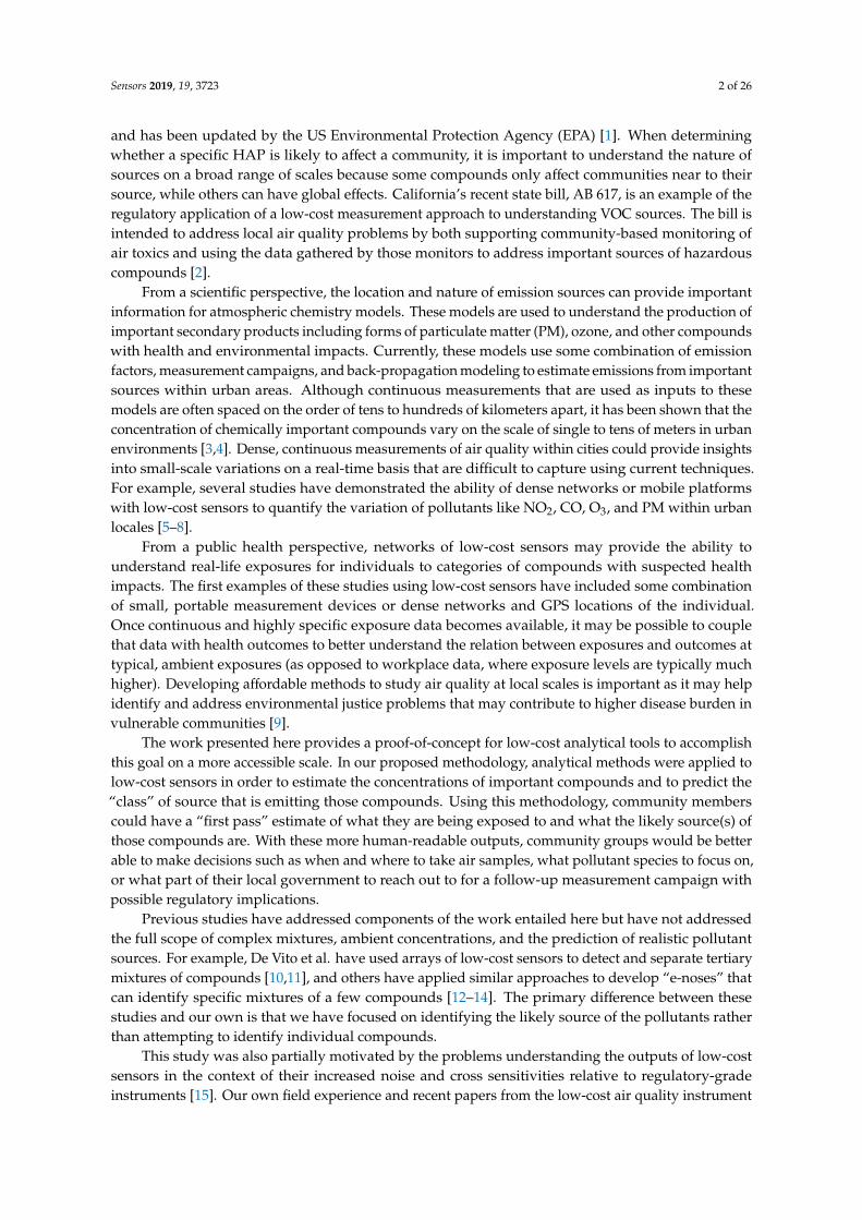
score as calculated using Equations (2)–(5), where n indicates the number of source classes and iindicates a specific source class. The notations tp, fp, tn, and fn represent the counts of true positives,false positives, true negatives, and false negatives, respectively. The F1 score is a popular metric whenunderstanding the performance of pattern recognition algorithms because it provides a balancedindication of both the precision and recall [60]. Precision can be understood as the fraction of timesthat a model is correct when it predicts that a source is present, and recall is the fraction of timesthat a source is present and the model “catches it”. The F1 score uses the harmonic mean of the twovalues, which more heavily penalizes poor performance in either metric, a consideration that becomesimportant when the prevalence of classes is not balanced. The F1 scores that were used for modelevaluation were those calculated on data that was left out of the training data for both regression andclassification and are shown in Table 3 for each combination of models.

F1,all =1n×

∑i=1:n

F1,i (2)

F1,i = 2×precisioni × recalliprecisioni + recalli

(3)

precisioni =tpi

tpi + f pi(4)

recalli =tpi

tpi + f ni(5)

Table 3. F1 Scores calculated for different combinations of regression and classification models.Calculated using Equations (2)–(6) on data that was held out for validation during model training.Cells are colored by the indicated score.

Classification Model

Logistic_class NeurNet_class RandFor_class SVMgaus_class SVMlin_class

Reg

ress

ion

Mod

el

FullLM 0.677 0.417 0.718 0.610 0.711

GaussProc 0.416 0.401 0.394 0.288 0.535

NeurNet 0.596 0.496 0.690 0.569 0.596

RandFor 0.332 0.442 0.479 0.578 0.556

RidgeLM 0.521 0.376 0.570 0.493 0.596

SelectLM 0.600 0.531 0.545 0.493 0.596

StepLM 0.695 0.502 0.619 0.614 0.616

3. Results

3.1. Regression Results

After training each model, the accuracy was measured as the root mean squared error (RMSE).Other analysis metrics like the Pearson correlation coefficient, that use the variance of the referencevalues were difficult to interpret because some folds of validation data consisted entirely of concentrationvalues that were exactly zero. These periods exist because some validation folds consisted of timeperiods when a compound was not being added to the chamber. The system used here does not havean online reference measurement of chamber concentrations, so it was assumed to be exactly zero.

Sensors 2019, 19, 3723 12 of 26

The RMSE values plotted in Figure 5 illustrate that the models perform acceptably but are generally notas accurate as has been achieved in the literature [5,27,37,52]. They also show that they are susceptibleto overfitting to various degrees as shown by the differences between the results on training data(dark colored boxes) and testing data (light boxes). The relatively poor performance that is reflectedin the RMSE values is also observed qualitatively when plotting the estimated concentrations versusreference values. For those plots, refer to Figure S2 in the Supplementary Materials.Sensors 2019, 19, x FOR PEER REVIEW 12 of 27

Figure 5. Boxplots of root mean squared error (RMSE) values (ppm) from each fold using each model

and species. Bars indicate the 25th and 75th percentile values, whiskers extend to values within 1.5

times that range from the median, and dots represent points outside of that range as calculated using

the GRAMM package implemented in MATLAB [61].

Interestingly, the variation between models when compared by their RMSE is not as great as one

might expect. It also appears that the regularization as applied to the ridge regression did not totally

address the problem of overtraining, as evidenced by the training RMSE values consistently

Methane

(Range: 1.5-15 ppm)

NO2

(Range: 0.33-1.4 ppm)

NMHC

(Range: 0.01-3.8 ppm)

Gasoline

(Range: 0.04-0.48 ppm) CO

(Range: 0.01-1.15 ppm)

CO2

(Range: 1-571 ppm)

Figure 5. Boxplots of root mean squared error (RMSE) values (ppm) from each fold using each modeland species. Bars indicate the 25th and 75th percentile values, whiskers extend to values within1.5 times that range from the median, and dots represent points outside of that range as calculatedusing the GRAMM package implemented in MATLAB [61].

Sensors 2019, 19, 3723 13 of 26

Interestingly, the variation between models when compared by their RMSE is not as great asone might expect. It also appears that the regularization as applied to the ridge regression did nottotally address the problem of overtraining, as evidenced by the training RMSE values consistentlyunderestimating the testing errors. This overtraining could indicate that the regularization didn’tbalance out the increased variance caused by the addition of temperature and humidity interactionfeatures introduced only for ridge regression. Neural nets and random forest regression typicallyperformed best in our study, possibly explained by their ability to encode complexities like interactions,changes in sensitivity over time, and nonlinearities in signal response.

The relatively poor performance of the models, as compared to the literature, may be partiallyexplained by design of the experiment. That is, this chamber study was designed to intentionallyintroduce a wide range of conditions containing known or suspected confounding gases at significantlyelevated levels. This wide range of sources and concentrations would be unlikely to occur in a singlelocation and it was, therefore, more challenging to accurately predict concentrations than in a typicalenvironment. Reference values are also calculated based on MFC flow rates, which introduces theassumption that the chamber is fully mixed and has reached steady-state concentrations equal to thatat the inlet. Both assumptions necessarily introduce additional uncertainties. Finally, the nature ofchamber studies produces relatively discrete values for each reference instead of the continuous valuesthat would be experienced in an ambient environment. This forces models to interpolate across arelatively wide range of conditions that are not seen in the training data; likely an important factor thatmay reduce the accuracy of the models.

3.2. Classification Results

At the end of the classification step, a set of values from 0 to 1 was output by each of theclassification models for each simulated source. These values indicated the model’s prediction thata source was or was not present at each time step. In a field application, these values would be theindication of the likelihood that a source was affecting the measured air quality.

The results of each combination of classification and regression model were evaluated usingempirical cumulative probability functions (CDFs) of the model outputs when a source was and wasnot present. An example of one of those plots is shown in Figure 6 for the best-performing set of models(“FullLM” and “RandFor_class”). By plotting a CDF of the output of the model, it was possible to seehow often a model correctly predicted the presence of a source (score ≥ 0.5) or absence of a source(score <0.5) when the source was present (blue line) and was not present (red line). The magnitude ofthe score also indicated how confident the model was in its prediction, so values closer to 0 or 1 wouldbe more useful to an end user because it would give a stronger indication that the source was actuallyabsent or present. For example, if the classifier output a value close to 1 for traffic emissions, the usercould be more confident that elevated concentrations were due to an influence of traffic pollution.In these plots, an ideal and omniscient model would roughly trace a box around the exterior; yielding ascore close to 0 for all points where a source was not being simulated (red), and close to 1 for all pointswhen a source was being simulated (blue). The CDF was plotted for classification models trained onboth the reference values and the estimated values output by regression models. This allowed us todetermine whether a model would or would not be able to separate the sources when given “perfect”concentration values. If not, then the model was unlikely to be useful when trained on less accurateestimates produced by regression models.


(a)

(b)

Figure 6. Example set of cumulative probability functions (CDFs) showing classification model

performance on both calibration (train) and validation (test) data. The red lines trace the CDF for test

cases where the source was not present (-), and blue lines illustrate the results when the source was

present (+). (a) shows performance using the reference gas concentrations as features, and (b) shows

performance for a combination of regression and classification models (in this case, FullLM and

RandFor_class).

Another analysis tool that was used to select models were the confusion matrices that are shown

in Figure 7 for each combination of regression and classification models. The confusion matrices

plotted here illustrate the fraction of times each source was identified as present when each of the

No Source, Training0

0

1

1


0

1

1

Low T Combustion, Training0

0

1

1

Gasoline Vapor, Training0

0

1

1

Heavy Exhaust, Training0

0

1

1

Natural Gas, Training0

0

1

1

00

1

1

No Source, Training


0

1

1


0

1

1

Low T Combustion, Validation0

0

1

1

Gasoline Vapor, Validation0

0

1

1

Heavy Exhaust, Validation0

0

1

1

Natural Gas, Validation0

0

1

1

00

1

1

No Source, Validation


0

1

1


0

1

1


0

1

1


0

1

1


0

1

1


0

1

1

00

1

1

No Source, Training


0

1

1


0

1

1


0

1

1


0

1

1


0

1

1


0

1

1

00

1

1


Score

F(x)

F(x)

F(x)

F(x)

F(x)

Score Score Score

F(x)

F(x)

F(x)

F(x)

F(x)


0

1

1


0

1

1


0

1

1


0

1

1


0

1

1


0

1

1

00

1

1

No Source, Training


0

1

1


0

1

1


0

1

1


0

1

1


0

1

1


0

1

1

00

1

1



0

1

1


0

1

1


0

1

1


0

1

1


0

1

1


0

1

1

00

1

1

No Source, Training


0

1

1


0

1

1


0

1

1


0

1

1


0

1

1


0

1

1

00

1

1


Score

F(x)

F(x)

F(x)

F(x)

F(x)

Score Score Score

F(x)

F(x)

F(x)

F(x)

F(x)

Figure 6. Example set of cumulative probability functions (CDFs) showing classification modelperformance on both calibration (train) and validation (test) data. The red lines trace the CDF for testcases where the source was not present (-), and blue lines illustrate the results when the source waspresent (+). (a) shows performance using the reference gas concentrations as features, and (b) showsperformance for a combination of regression and classification models (in this case, FullLM andRandFor_class).


Figure 7. Confusion matrices showing the classification success on validation data. Each chart shows the results of a combination of classification (columns) and

regression (rows) models. Within each confusion matrix, the reference class is shown on the “y” axis and predicted class is indicated on the “x” axis. Lighter colors

indicate higher values, ranging from 0 to 1, which correspond to the fraction of times that a source was predicted when a source was being simulated.

Figure 7. Confusion matrices showing the classification success on validation data. Each chart shows the results of a combination of classification (columns) andregression (rows) models. Within each confusion matrix, the reference class is shown on the “y” axis and predicted class is indicated on the “x” axis. Lighter colorsindicate higher values, ranging from 0 to 1, which correspond to the fraction of times that a source was predicted when a source was being simulated.

Sensors 2019, 19, 3723 16 of 26

Another analysis tool that was used to select models were the confusion matrices that are shownin Figure 7 for each combination of regression and classification models. The confusion matricesplotted here illustrate the fraction of times each source was identified as present when each of thesources was being simulated. Confusion matrices are useful because they help us to understand whattypes of mistakes the model is making. For example, the top row of each confusion matrix shows thefraction of times that a model predicted that a source was present when no source was being activelysimulated. A confusion matrix for an ideal model would be a matrix with the value of 1 along thediagonal and 0 elsewhere, indicating that it predicted the correct source every time. As mentionedbefore, the threshold was set as 0.5 for each model output, and each model was trained independently,so it was possible that multiple sources were predicted for a single timestep. This functionality wasintentional because it would allow for the identification of multiple simultaneous sources, a situationthat is likely to occur in reality.

Several of the models had problems with confusion between low- and high-temperaturecombustion that should have been easily differentiated by the presence of NOx. After reviewing thedata, it appears that the NO2 electrochemical sensor failed approximately 2/3 of the way through thetest matrix, likely hampering the ability of regression models to learn its importance in predicting NO2

concentrations. Interestingly, the regression model that used all of the sensor signals was the one thatproduced the best inputs to the classifier models. This may be because it did not discard other sensorsthat would have been possibly less useful for the regression of NO2 but that also did not fail near theend of the test.

4. Discussion


Using the criterion of maximum F1 score as defined in Equations (2)–(4), the best performancewas accomplished by using the full multiple linear model (FullLM) to produce concentration estimatesfor a set of random forest models (RandFor_class) that estimated the sources. The performance ofthis pair is highlighted in Figure 8, which shows that the models were most effective at identifyinggasoline vapors, and the second most successful classification was for natural gas emissions. The mostcommon mistakes made by the model were confusion between low-temperature combustion andheavy exhaust. This makes intuitive sense because the only differentiating factor in this study was thepresence of NO2 during heavy exhaust emissions, a compound that the regression models struggled toaccurately predict.


4. Discussion


Using the criterion of maximum F1 score as defined in Equations (2)–(4), the best performance

was accomplished by using the full multiple linear model (FullLM) to produce concentration

estimates for a set of random forest models (RandFor_class) that estimated the sources. The

performance of this pair is highlighted in Figure 8, which shows that the models were most effective

at identifying gasoline vapors, and the second most successful classification was for natural gas

emissions. The most common mistakes made by the model were confusion between low-temperature

combustion and heavy exhaust. This makes intuitive sense because the only differentiating factor in

this study was the presence of NO2 during heavy exhaust emissions, a compound that the regression

models struggled to accurately predict.

Table 3. F1 Scores calculated for different combinations of regression and classification models.

Calculated using Equations (2)–(6) on data that was held out for validation during model training.

Cells are colored by the indicated score.

Classification Model

Logistic_class NeurNet_class RandFor_class SVMgaus_class SVMlin_class

Reg

ress

ion

Mo

del

FullLM 0.677 0.417 0.718 0.610 0.711

GaussProc 0.416 0.401 0.394 0.288 0.535

NeurNet 0.596 0.496 0.690 0.569 0.596

RandFor 0.332 0.442 0.479 0.578 0.556

RidgeLM 0.521 0.376 0.570 0.493 0.596

SelectLM 0.600 0.531 0.545 0.493 0.596

StepLM 0.695 0.502 0.619 0.614 0.616

Figure 8. Confusion matrix for the “best” combination of models as judged by the F1 score as

calculated using validation data. This combination involved regression using all linear models and

then random forest classification trees.

4.2. Sensor Importance for Different Compounds

The sensors that were most influential when estimating the concentration of different gases was

investigated by probing parameters from a few different regression models. This investigation will

hopefully inform the design of future sensor arrays that are targeting some or all of the compounds

discussed here. Specifically, we explored the sensor signals that were selected by stepwise regression,

the unbiased importance measures for sensors from the random forest regression models, and the

standardized ridge trace generated when fitting ridge regression models. By looking at which sensors

were especially important to different models, it was possible to see which sensors were likely to be

truly important for estimating the concentration of a gas.

4.2.1. Terms Selected by Stepwise Regression

Figure 8. Confusion matrix for the “best” combination of models as judged by the F1 score as calculatedusing validation data. This combination involved regression using all linear models and then randomforest classification trees.

4.2. Sensor Importance for Different Compounds

The sensors that were most influential when estimating the concentration of different gases wasinvestigated by probing parameters from a few different regression models. This investigation willhopefully inform the design of future sensor arrays that are targeting some or all of the compounds

Sensors 2019, 19, 3723 17 of 26

discussed here. Specifically, we explored the sensor signals that were selected by stepwise regression,the unbiased importance measures for sensors from the random forest regression models, and thestandardized ridge trace generated when fitting ridge regression models. By looking at which sensorswere especially important to different models, it was possible to see which sensors were likely to betruly important for estimating the concentration of a gas.

4.2.1. Terms Selected by Stepwise Regression

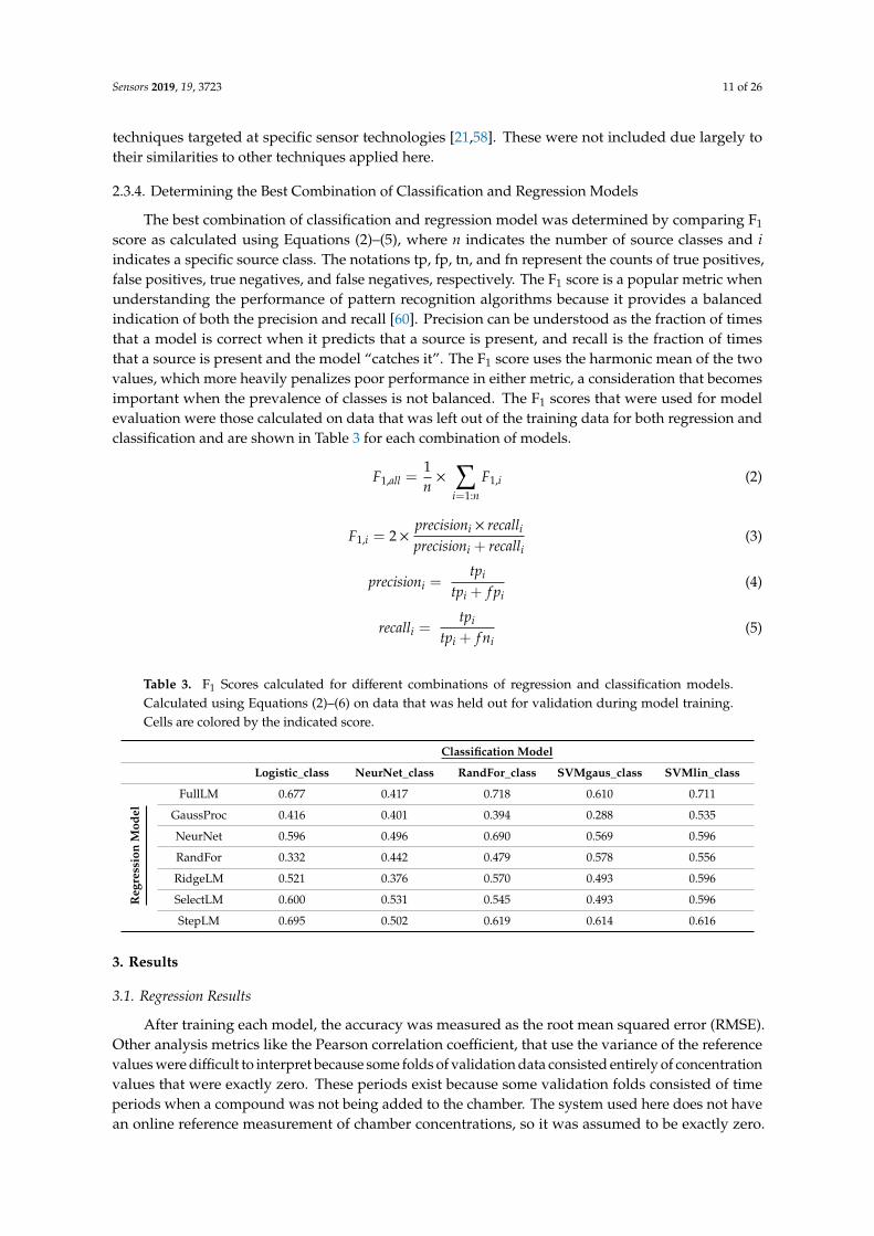
Figure 9 shows the sensors selected by stepwise linear regression for each compound of interestwhere the boxplots indicate the statistical importance of those sensors when they were selected.Many of the terms selected algorithmically match the sensors that we have used based on previousexperience [52,62], although there were a few surprises that would suggest further investigation.For example, terms that were expected were the inclusion of the Figaro 2600 and 2602 for the detectionof methane and nonmethane hydrocarbons (NMHC). The importance of the Baseline Mocon sensor forgasoline was also expected, as it is one of the few sensors that our research group has used to detectheavy hydrocarbons at sub ppm levels. Finally, the sole selection of the NDIR sensor for CO2 fromNLT was expected as this technology is generally quite robust to cross-interferences and has beenused successfully before in other studies. Some of the unexpected terms were the inclusion of the CO2

sensor for indication of CO and NO2, although this is likely because NO2 was only ever present whenCO2 was also present, although not always at the same ratios, and the reverse was not true. CO isinteresting in that there were some test points where only CO was present, although it is possible thatthere were not enough to counteract the more common correlation between the two compounds. It’salso interesting that the gasoline models consistently selected the Figaro 4161, which is an older metaloxide sensor that was marketed for the detection of CO2. Other sensors were selected for inclusionin only one or two of the cross-validation folds for NO2, CO, and NMHC, which indicates that theirinclusion is not reliable and may be caused by a correlation unrelated to sensitivities.


Figure 9 shows the sensors selected by stepwise linear regression for each compound of interest

where the boxplots indicate the statistical importance of those sensors when they were selected. Many

of the terms selected algorithmically match the sensors that we have used based on previous

experience [52,62], although there were a few surprises that would suggest further investigation. For

example, terms that were expected were the inclusion of the Figaro 2600 and 2602 for the detection

of methane and nonmethane hydrocarbons (NMHC). The importance of the Baseline Mocon sensor

for gasoline was also expected, as it is one of the few sensors that our research group has used to

detect heavy hydrocarbons at sub ppm levels. Finally, the sole selection of the NDIR sensor for CO2

from NLT was expected as this technology is generally quite robust to cross-interferences and has

been used successfully before in other studies. Some of the unexpected terms were the inclusion of

the CO2 sensor for indication of CO and NO2, although this is likely because NO2 was only ever

present when CO2 was also present, although not always at the same ratios, and the reverse was not

true. CO is interesting in that there were some test points where only CO was present, although it is

possible that there were not enough to counteract the more common correlation between the two

compounds. It’s also interesting that the gasoline models consistently selected the Figaro 4161, which

is an older metal oxide sensor that was marketed for the detection of CO2. Other sensors were selected

for inclusion in only one or two of the cross-validation folds for NO2, CO, and NMHC, which

indicates that their inclusion is not reliable and may be caused by a correlation unrelated to

sensitivities.

Figure 9. Frequency that each term was selected by stepwise regression for each pollutant from all

cross-validation folds. When an interaction term was selected, it was named with “Sensor1:Sensor2”

where “Sensor1” and Sensor2” are replaced with the sensor names.

4.2.2. Random Forest Unbiased Importance Estimates

The random forests were trained such that they determined the variable to split at each node by

using the interaction-curvature test as implemented by the MATLAB function “fitrtree”. This method

allows the model to account for interactions between variables and produces unbiased estimates of

the change in mean squared error (MSE) associated with the variable selected to split at each node.

Because the decision of which variable to split on is evaluated for each tree at each node using

different subsets of the full set of variables, importance estimates are generated for every variable

and are determined on a wide range of subsets of the data. The ten most important variables—in this

case sensor signals—for each compound are shown in Figure 10.

Figure 9. Frequency that each term was selected by stepwise regression for each pollutant from allcross-validation folds. When an interaction term was selected, it was named with “Sensor1:Sensor2”where “Sensor1” and Sensor2” are replaced with the sensor names.

Sensors 2019, 19, 3723 18 of 26

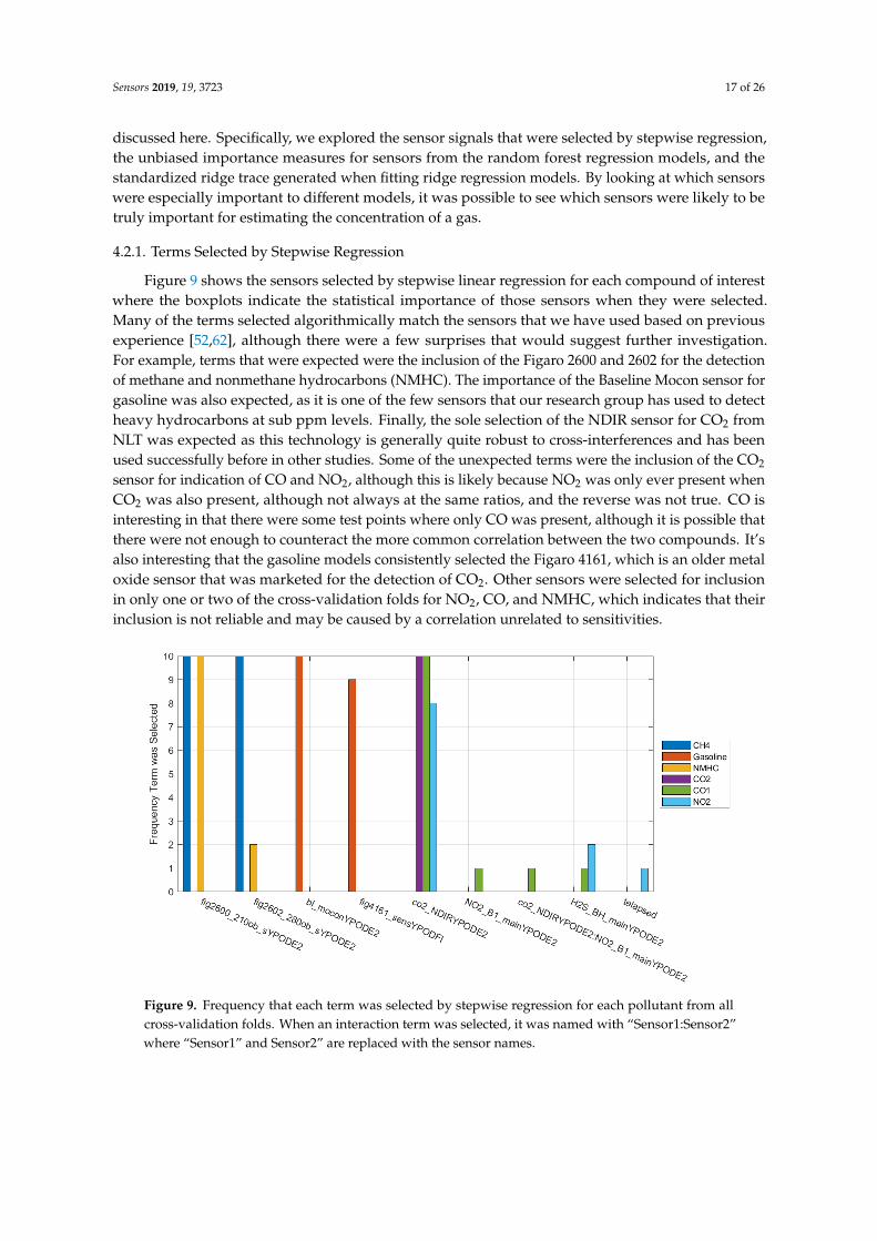
4.2.2. Random Forest Unbiased Importance Estimates

The random forests were trained such that they determined the variable to split at each node byusing the interaction-curvature test as implemented by the MATLAB function “fitrtree”. This methodallows the model to account for interactions between variables and produces unbiased estimates ofthe change in mean squared error (MSE) associated with the variable selected to split at each node.Because the decision of which variable to split on is evaluated for each tree at each node using differentsubsets of the full set of variables, importance estimates are generated for every variable and aredetermined on a wide range of subsets of the data. The ten most important variables—in this casesensor signals—for each compound are shown in Figure 10.

For NO2, we once again see that none of the sensors were selected to have a strong importance.This again is likely at least partly due to the failure of the NO2 sensor part way through testing. This isreflected in the high ranking of the elapsed time (“telapsed”) variable, as it would help separate thepoint of failure for that sensor. The H2S electrochemical sensor is again among the more importantinputs, reinforcing the hypothesis that it is at least partially sensitive to NO2. Interestingly, the NO2

sensor does feature prominently in the CO importance plot. It is possible that the individual treesmaking up the random forest learned to screen the NO2 sensor when it had failed so as to be ableto still use its common association with NO2, although it is not clear why that would be true whenestimating CO and not NO2.


For NO2, we once again see that none of the sensors were selected to have a strong importance.

This again is likely at least partly due to the failure of the NO2 sensor part way through testing. This

is reflected in the high ranking of the elapsed time (“telapsed”) variable, as it would help separate

the point of failure for that sensor. The H2S electrochemical sensor is again among the more important

inputs, reinforcing the hypothesis that it is at least partially sensitive to NO2. Interestingly, the NO2

sensor does feature prominently in the CO importance plot. It is possible that the individual trees

making up the random forest learned to screen the NO2 sensor when it had failed so as to be able to

still use its common association with NO2, although it is not clear why that would be true when

estimating CO and not NO2.

Both the methane and nonmethane hydrocarbon (NMHC) models are dominated by the Figaro

2600, which is the sensor that we have shown to be effective for similar applications [52,62]. It is

possible that the NMHC are simply taking advantage of the partial correlation of NMHC with

methane and not actually recording a sensitivity of the Figaro 2600 to other NMHC. This is reinforced

by the lower ranking of the 2600 when regressing gasoline concentrations. In this model, the Baseline

Mocon PID sensor and Figaro 2602 are selected, and their selection matches our experience with

detecting heavier hydrocarbons. The elapsed time variable is relatively important here, which

matches a drift in the Figaro 2602 that was noticed when reviewing the sensor values over the full

test period.

The CO2 model is also dominated by the NDIR CO2 sensor from ELT, another instance where

the models match expectations [19,52]. The gasoline model is also again dominated by the Baseline

Mocon PID sensor and the Figaro 2602, which are two sensors that we have used to study those

compounds in the past. The MICS-5121wp sensor by e2v is also relatively important, and it, too, is a

sensor targeted at the detection of VOCs.

(a) (b)

(c) (d)

Figure 10. Cont.


(e) (f)

Figure 10. Box plots of the top 10 predictors sorted by out-of-bag importance estimates for each

regressed pollutant. These pollutants were (a) NO2, (b) CO, (c) NMHC, (d) Gasoline, (e) CO2, and (f)

CH4. Boxes indicate the variation in the predictor importance when models were trained on different

cross-validation folds.

4.2.3. Standardized Ridge Regression Coefficients

The use of ridge regression offered an opportunity to review which sensors contributed to

models when using regularization to avoid overfitting. Because of this regularization, more initial

terms could be included; in this case, interactions between each sensor and temperature, humidity,

and both temperature and humidity were included in the input dataset. These are denoted by

appending “:T”, “:H”, or “:T:H”, respectively, to the end of the sensor name. The methodology here

initially used a range of regularization coefficients to produce a “ridge trace” plot that showed the

standardized weight assigned to each variable as a function of that regularization coefficient (see

Figure 11). By reviewing the ridge trace produced for each pollutant, it was possible to select a

regularization coefficient that seemed to be an appropriate combination of reducing variance while

avoiding underfitting. For this study, that value seemed to typically range between 1 and 10 for all

pollutants, so a value of 5 was applied to all models for consistency and to avoid over-learning that

hyperparameter. The ridge trace plots for each compound provide another insight into which sensors

were important enough to the model that its importance to the model outweighed all but extreme

values of regularization. This is indicated by weight values that are relatively high and stable, even

at high levels of regularization (the right side of the plot).

In the NO2 ridge trace, most of the weights collapsed toward zero as regularization was

increased, indicating that none were especially strongly correlated with NO2. That said, the H2S

sensor was relatively resistant to regularization, indicating that it may have some sensitivity to NO2.

The CO2 NDIR sensor term with temperature interaction term is also quite stable, although this may

simply indicate that NO2 was sometimes co-emitted with CO2. It is important to again note that the

NO2 sensor included in the study appears to have failed during the second half of testing, likely

explaining its absence from this plot.

For CO, a strong dependence was seen with the NO2 sensor, although this may again be caused

by the fact that NO2 was sometimes released at the same time as CO. The CO2 NDIR sensor is also

relatively resistant to regularization, but this may be caused by the same phenomena. Interestingly,

the electrochemical ozone sensor (with temperature interaction) was relatively strongly and

negatively represented in the ridge traces. This may indicate that the catalytic surface on the ozone

sensor is somewhat sensitive to carbon monoxide, although the electrochemical cell would be

operating in “reverse” as ozone is an oxidizing agent and CO is reducing.

Nonmethane hydrocarbons (NMHC) seem to have been dominated by their inclusion as a

component of some of the simulated natural gas emissions, as both Figaro 2600s were strongly

Figure 10. Box plots of the top 10 predictors sorted by out-of-bag importance estimates for eachregressed pollutant. These pollutants were (a) NO2, (b) CO, (c) NMHC, (d) Gasoline, (e) CO2,and (f) CH4. Boxes indicate the variation in the predictor importance when models were trained ondifferent cross-validation folds.

Both the methane and nonmethane hydrocarbon (NMHC) models are dominated by the Figaro2600, which is the sensor that we have shown to be effective for similar applications [52,62]. It ispossible that the NMHC are simply taking advantage of the partial correlation of NMHC with methaneand not actually recording a sensitivity of the Figaro 2600 to other NMHC. This is reinforced by thelower ranking of the 2600 when regressing gasoline concentrations. In this model, the Baseline MoconPID sensor and Figaro 2602 are selected, and their selection matches our experience with detectingheavier hydrocarbons. The elapsed time variable is relatively important here, which matches a drift inthe Figaro 2602 that was noticed when reviewing the sensor values over the full test period.

The CO2 model is also dominated by the NDIR CO2 sensor from ELT, another instance where themodels match expectations [19,52]. The gasoline model is also again dominated by the Baseline MoconPID sensor and the Figaro 2602, which are two sensors that we have used to study those compounds inthe past. The MICS-5121wp sensor by e2v is also relatively important, and it, too, is a sensor targetedat the detection of VOCs.

4.2.3. Standardized Ridge Regression Coefficients

The use of ridge regression offered an opportunity to review which sensors contributed to modelswhen using regularization to avoid overfitting. Because of this regularization, more initial termscould be included; in this case, interactions between each sensor and temperature, humidity, and bothtemperature and humidity were included in the input dataset. These are denoted by appending “:T”,“:H”, or “:T:H”, respectively, to the end of the sensor name. The methodology here initially used arange of regularization coefficients to produce a “ridge trace” plot that showed the standardized weightassigned to each variable as a function of that regularization coefficient (see Figure 11). By reviewingthe ridge trace produced for each pollutant, it was possible to select a regularization coefficient thatseemed to be an appropriate combination of reducing variance while avoiding underfitting. For thisstudy, that value seemed to typically range between 1 and 10 for all pollutants, so a value of 5 wasapplied to all models for consistency and to avoid over-learning that hyperparameter. The ridge traceplots for each compound provide another insight into which sensors were important enough to themodel that its importance to the model outweighed all but extreme values of regularization. This isindicated by weight values that are relatively high and stable, even at high levels of regularization(the right side of the plot).

In the NO2 ridge trace, most of the weights collapsed toward zero as regularization was increased,indicating that none were especially strongly correlated with NO2. That said, the H2S sensor was

Sensors 2019, 19, 3723 20 of 26

relatively resistant to regularization, indicating that it may have some sensitivity to NO2. The CO2

NDIR sensor term with temperature interaction term is also quite stable, although this may simplyindicate that NO2 was sometimes co-emitted with CO2. It is important to again note that the NO2

sensor included in the study appears to have failed during the second half of testing, likely explainingits absence from this plot.

For CO, a strong dependence was seen with the NO2 sensor, although this may again be causedby the fact that NO2 was sometimes released at the same time as CO. The CO2 NDIR sensor is alsorelatively resistant to regularization, but this may be caused by the same phenomena. Interestingly,the electrochemical ozone sensor (with temperature interaction) was relatively strongly and negativelyrepresented in the ridge traces. This may indicate that the catalytic surface on the ozone sensor issomewhat sensitive to carbon monoxide, although the electrochemical cell would be operating in“reverse” as ozone is an oxidizing agent and CO is reducing.

Nonmethane hydrocarbons (NMHC) seem to have been dominated by their inclusion as acomponent of some of the simulated natural gas emissions, as both Figaro 2600s were stronglyweighted even with high regularization. Temperature itself was also selected, although it is not clearwhy this was selected rather than the terms that included temperature interactions.


weighted even with high regularization. Temperature itself was also selected, although it is not clear

why this was selected rather than the terms that included temperature interactions.

Gasoline vapors produced a significantly different plot from NMHC, likely because they were

not co-emitted with methane and were not dominated by the ethane and propane signals from the

simulated natural gas emissions. These vapors were well captured by the Baseline Mocon PID sensor

that is designed to quantify gaseous hydrocarbons. Interestingly, the parameter of just this sensor

and the parameter with the interaction of this sensor with temperature and humidity were both

selected strongly. This may indicate that the sensor has some sensitivity to environmental parameters

as well as the mixture itself. The Figaro 2602 with humidity interaction was also selected strongly,

which is an expected result as these vapors are the target of the 2602 and humidity is known to affect

metal oxide sensors. One of the pressure sensors (BME) was also selected with almost as much weight

as the Figaro 2600 sensor. After reviewing the data, we determined that this was due to a spurious

correlation with pressure in the chamber, which was not controlled.

For CO2, several of the Figaro 2600 sensors were selected, although it is not clear whether that is

representative of a true cross-sensitivity to CO2. It is, for example, possible that these are actually

cross-sensitive to CO, which was co-emitted with CO2 in some of the testing. The CO2 NDIR sensor

on one of the pods was selected, although not as distinctly as one might have predicted, based on the

typical sensitivity of these sensors.

Finally, for methane, the Figaro 2600 sensor term was selected most strongly at higher levels of

regularization. The Figaro 2600 sensor that was installed on the ancillary board and which operated

at a slightly different operating temperature was also selected somewhat at a similar level to the

Baseline Mocon PID sensor. Both BME pressure sensors were again selected, representing an

incidental correlation with pressure.

(a) (b)

(c) (d)

Figure 11. Cont.


(e) (f)

Figure 11. Summary of ridge traces of the top 10 most important parameters from the regression of

each pollutant. These pollutants were (a) NO2, (b) CO, (c) NMHC, (d) Gasoline, (e) CO2, and (f) CH4.

Weight magnitude should not be compared between compounds because they scale with the

concentration values. Interactions with temperature and/or humidity are indicated by “:T”, “:H”, or

“:T:H, respectively. Colors indicate the sensor and are sorted from largest to smallest importance at

high regularization. Dashed lines illustrate the ridge trace for each cross-validation fold, and the solid

lines illustrate the median value for all folds. The x-axis of each plot indicates the ridge parameter

(regularization strength), and the y-axis indicates the unbiased parameter weight. Larger absolute

values indicate a stronger importance of that sensor, especially at larger values of the ridge parameter.

5. Conclusions

In this study, we have shown the ability of current modeling and machine learning techniques

to quantify several trace gases and identify likely sources for those trace gases using an array of low-

cost sensors. The best combination of regression and classification methods for source identification

was a linear regression using every sensor in the array followed by a random forest of classification

trees. The F1 score as calculated on data that was held out during optimization and model fitting was

0.718, indicating a relatively strong combination of accuracy and precision. The success of these

models was an unexpected result as our previous work suggested that a linear regression model with

every sensor signal was likely to overfit and perform poorly on validation data. We also initially

suspected that this model would fail to capture the interactions between sensors and environmental

parameters like temperature and humidity. Indeed, as far as regression accuracy, many of the other

regression models outperformed this model when predicting on validation data. That said, it is

possible that the random forest classifier model was able to encode the interferences that would have

been normally captured by the regression model while also taking advantage of signals that would

have been removed or reduced by other regression models. If true, the omission of the regression

step could be considered, although it would greatly increase the computational power required to

train and apply the random forest classifier models.

In this study, we also reviewed the variable importance from three different regression models

to investigate the value of sensors when quantifying different pollutants of interest. Although there

were some issues caused by sensor failure, these may provide valuable insight to researchers

designing the next generation of sensor platforms.

Going forward, it will be important to validate these methods in more realistic environments as

chamber calibrations are known to be imperfect representations of field performance [18,63]. One

example of a study that could provide valuable insights would be the placement of this sensor array

in regions where different sources are likely to dominate, e.g., immediately next to a highway onramp

and then next to a well during completion. By collecting data in these locations as well as e.g., rural

sites, it would be possible to determine how well the identification of sources might function in

situations where the qualitative levels are known. This has been demonstrated by Molino and others

for the detection of single sources [26].

Figure 11. Summary of ridge traces of the top 10 most important parameters from the regression of eachpollutant. These pollutants were (a) NO2, (b) CO, (c) NMHC, (d) Gasoline, (e) CO2, and (f) CH4. Weightmagnitude should not be compared between compounds because they scale with the concentrationvalues. Interactions with temperature and/or humidity are indicated by “:T”, “:H”, or “:T:H, respectively.Colors indicate the sensor and are sorted from largest to smallest importance at high regularization.Dashed lines illustrate the ridge trace for each cross-validation fold, and the solid lines illustratethe median value for all folds. The x-axis of each plot indicates the ridge parameter (regularizationstrength), and the y-axis indicates the unbiased parameter weight. Larger absolute values indicate astronger importance of that sensor, especially at larger values of the ridge parameter.

Gasoline vapors produced a significantly different plot from NMHC, likely because they werenot co-emitted with methane and were not dominated by the ethane and propane signals from thesimulated natural gas emissions. These vapors were well captured by the Baseline Mocon PID sensorthat is designed to quantify gaseous hydrocarbons. Interestingly, the parameter of just this sensor andthe parameter with the interaction of this sensor with temperature and humidity were both selectedstrongly. This may indicate that the sensor has some sensitivity to environmental parameters as well asthe mixture itself. The Figaro 2602 with humidity interaction was also selected strongly, which is anexpected result as these vapors are the target of the 2602 and humidity is known to affect metal oxidesensors. One of the pressure sensors (BME) was also selected with almost as much weight as the Figaro2600 sensor. After reviewing the data, we determined that this was due to a spurious correlation withpressure in the chamber, which was not controlled.

For CO2, several of the Figaro 2600 sensors were selected, although it is not clear whether thatis representative of a true cross-sensitivity to CO2. It is, for example, possible that these are actuallycross-sensitive to CO, which was co-emitted with CO2 in some of the testing. The CO2 NDIR sensor onone of the pods was selected, although not as distinctly as one might have predicted, based on thetypical sensitivity of these sensors.

Finally, for methane, the Figaro 2600 sensor term was selected most strongly at higher levels ofregularization. The Figaro 2600 sensor that was installed on the ancillary board and which operatedat a slightly different operating temperature was also selected somewhat at a similar level to theBaseline Mocon PID sensor. Both BME pressure sensors were again selected, representing an incidentalcorrelation with pressure.

5. Conclusions

In this study, we have shown the ability of current modeling and machine learning techniques toquantify several trace gases and identify likely sources for those trace gases using an array of low-costsensors. The best combination of regression and classification methods for source identification was alinear regression using every sensor in the array followed by a random forest of classification trees.

Sensors 2019, 19, 3723 22 of 26

The F1 score as calculated on data that was held out during optimization and model fitting was 0.718,indicating a relatively strong combination of accuracy and precision. The success of these models wasan unexpected result as our previous work suggested that a linear regression model with every sensorsignal was likely to overfit and perform poorly on validation data. We also initially suspected thatthis model would fail to capture the interactions between sensors and environmental parameters liketemperature and humidity. Indeed, as far as regression accuracy, many of the other regression modelsoutperformed this model when predicting on validation data. That said, it is possible that the randomforest classifier model was able to encode the interferences that would have been normally capturedby the regression model while also taking advantage of signals that would have been removed orreduced by other regression models. If true, the omission of the regression step could be considered,although it would greatly increase the computational power required to train and apply the randomforest classifier models.

In this study, we also reviewed the variable importance from three different regression models toinvestigate the value of sensors when quantifying different pollutants of interest. Although there weresome issues caused by sensor failure, these may provide valuable insight to researchers designing thenext generation of sensor platforms.

Going forward, it will be important to validate these methods in more realistic environmentsas chamber calibrations are known to be imperfect representations of field performance [18,63].One example of a study that could provide valuable insights would be the placement of this sensorarray in regions where different sources are likely to dominate, e.g., immediately next to a highwayonramp and then next to a well during completion. By collecting data in these locations as well as e.g.,rural sites, it would be possible to determine how well the identification of sources might function insituations where the qualitative levels are known. This has been demonstrated by Molino and othersfor the detection of single sources [26].

There are also other analysis techniques that could be used to possibly improve the resultspresented here. Specifically, combining the models into ensembles for both classification and regression,the ensembles could improve overall results by combining models that make “decisions” in differentways and are, therefore, less likely to make the same types of mistakes. The use of generativeclassification models could also improve the identification of sources. These models learn thecharacteristics of different classes instead of learning to separate one class from another. This type ofclassifier generally performs better on smaller training data sets. This would be important for worklike that presented here because any economical calibration strategy will always represent a smalltraining set relative to the range of environments in which a sensor could be deployed.

Finally, many sensors were not available for inclusion in this array due to limited availability.Including new sensors in the array could fill in gaps that were not covered by the relatively limitedvariety of sensors here. These new inputs could involve similar sensors operated in new ways,e.g., temperature-cycled MOx sensors that have been shown to improve sensitivity to VOCs and othergases [21,35,64]. It could also include sensors with wildly different operating principles like micro-GCs(gas chomatographs) [27] or with new targets like the low-cost PM sensors that could also be useful inthe differentiation of sources.

Supplementary Materials: The following are available online at http://www.mdpi.com/1424-8220/19/17/3723/s1,Section S.1: Details of the Computational Methods as Applied Here, Table S1: Additional Sensor Information,Table S2: Full Listing of Test Points, Figure S2: Additional Model Performance Plots. References [65,66] are citedin the supplementary materials.

Author Contributions: Conceptualization, J.T., A.C.-O., and M.H.; methodology, J.T., A.C.-O., and M.H.; validation,J.T. and M.H.; formal analysis, J.T. and A.C.-O.; investigation, J.T.; data curation, J.T.; writing—original draftpreparation, J.T.; writing—review and editing, J.T., A.C.-O., and M.H.; visualization, J.T.; supervision, M.H.;funding acquisition, M.H.

Funding: This research is supported in part by the AirWaterGas Sustainability Research Network funded bythe National Science Foundation under Grant No. CBET-1240584. Any opinion, findings, and conclusions or

http://www.mdpi.com/1424-8220/19/17/3723/s1

Sensors 2019, 19, 3723 23 of 26

recommendations expressed in this dissertation are those of the author and do not necessarily reflect the views ofthe National Science Foundation.

Acknowledgments: Additional thanks to Evan Coffey and Joanna Gordon-Casey for their input and supportduring the design and testing phases of this work and to Gustavo Aguirre Jr. and Sue Chiang for their inputregarding the pollutant sources of interest for Los Angeles area communities. Publication of this article wasfunded by the University of Colorado Boulder Libraries Open Access Fund.

Conflicts of Interest: The authors declare no conflict of interest.

References

1. US EPA. Integrated Urban Air Toxics Strategy. Available online: https://www.epa.gov/urban-air-toxics/integrated-urban-air-toxics-strategy (accessed on 25 September 2018).

2. Garcia, C. AB-617 Nonvehicular Air Pollution: Criteria Air Pollutants and Toxic Air Contaminants.2017. Available online: https://leginfo.legislature.ca.gov/faces/billTextClient.xhtml?bill_id=201720180AB617(accessed on 18 October 2018).

3. Cheadle, L.; Deanes, L.; Sadighi, K.; Casey, J.G.; Collier-Oxandale, A.; Hannigan, M. Quantifyingneighborhood-scale spatial variations of ozone at open space and urban sites in Boulder, Colorado usinglow-cost sensor technology. Sensors 2017, 17, 2072. [CrossRef] [PubMed]

4. Tan, Y.; Lipsky, E.M.; Saleh, R.; Robinson, A.L.; Presto, A.A. Characterizing the spatial variation of airpollutants and the contributions of high emitting vehicles in Pittsburgh, PA. Environ. Sci. Technol. 2014, 48,14186–14194. [CrossRef] [PubMed]

5. Mead, M.I.; Popoola, O.A.M.; Stewart, G.B.; Landshoff, P.; Calleja, M.; Hayes, M.; Baldovi, J.J.; McLeod, M.W.;Hodgson, T.F.; Dicks, J.; et al. The use of electrochemical sensors for monitoring urban air quality in low-cost,high-density networks. Atmos. Environ. 2013, 70, 186–203. [CrossRef]

6. Penza, M.; Suriano, D.; Pfister, V.; Prato, M.; Cassano, G. Urban air quality monitoring with networkedlow-cost sensor-systems. Proceedings 2017, 1, 573. [CrossRef]

7. Popoola, O.A.M.; Carruthers, D.; Lad, C.; Bright, V.B.; Mead, M.I.; Stettler, M.E.J.; Saffell, J.R.; Jones, R.L.Use of networks of low cost air quality sensors to quantify air quality in urban settings. Atmos. Environ.2018, 194, 58–70. [CrossRef]

8. Sadighi, K.; Coffey, E.; Polidori, A.; Feenstra, B.; Lv, Q.; Henze, D.K.; Hannigan, M. Intra-urban spatialvariability of surface ozone in Riverside, CA: Viability and validation of low-cost sensors. Atmos. Measur.Tech. 2018, 11, 1777–1792. [CrossRef]

9. Martenies, S.E.; Milando, C.W.; Williams, G.O.; Batterman, S.A. Disease and health inequalities attributableto air pollutant exposure in Detroit, Michigan. Int. J. Environ. Res. Public Health 2017, 14, 1243. [CrossRef][PubMed]

10. De Vito, S.; Castaldo, A.; Loffredo, F.; Massera, E.; Polichetti, T.; Nasti, I.; Vacca, P.; Quercia, L.; Di Francia, G.Gas concentration estimation in ternary mixtures with room temperature operating sensor array usingtapped delay architectures. Sens. Actuators B Chem. 2007, 124, 309–316. [CrossRef]

11. De Vito, S.; Piga, M.; Martinotto, L.; Di Francia, G. CO, NO2 and NOx urban pollution monitoring withon-field calibrated electronic nose by automatic bayesian regularization. Sens. Actuators B Chem. 2009, 143,182–191. [CrossRef]

12. Akamatsu, T.I.T.; Tsuruta, A.; Shin, W. Selective detection of target volatile organic compounds incontaminated humid air using a sensor array with principal component analysis. Sensors 2017, 17, 1662.[CrossRef]

13. Aleixandre, M.; Sayago, I.; Horrillo, M.C.; Fernández, M.J.; Arés, L.; García, M.; Santos, J.P.; Gutiérrez, J.Analysis of neural networks and analysis of feature selection with genetic algorithm to discriminate amongpollutant gas. Sens. Actuators B Chem. 2004, 103, 122–128. [CrossRef]

14. Capone, S.; Siciliano, P.; Bârsan, N.; Weimar, U.; Vasanelli, L. Analysis of CO and CH4 gas mixtures by usinga micromachined sensor array. Sens. Actuators B Chem. 2001, 78, 40–48. [CrossRef]

15. Clements, A.L.; Griswold, W.G.; Rs, A.; Johnston, J.E.; Herting, M.M.; Thorson, J.; Collier-Oxandale, A.;Hannigan, M. Low-cost air quality monitoring tools: from research to practice (a workshop summary).Sensors 2017, 17, 2478. [CrossRef] [PubMed]

https://www.epa.gov/urban-air-toxics/integrated-urban-air-toxics-strategy

https://www.epa.gov/urban-air-toxics/integrated-urban-air-toxics-strategy

https://leginfo.legislature.ca.gov/faces/billTextClient.xhtml?bill_id=201720180AB617

http://dx.doi.org/10.3390/s17092072

http://www.ncbi.nlm.nih.gov/pubmed/28891962

http://dx.doi.org/10.1021/es5034074


http://dx.doi.org/10.1016/j.atmosenv.2012.11.060

http://dx.doi.org/10.3390/proceedings1040573


http://dx.doi.org/10.5194/amt-11-1777-2018

http://dx.doi.org/10.3390/ijerph14101243


http://dx.doi.org/10.1016/j.snb.2006.12.039


http://dx.doi.org/10.3390/s17071662


http://dx.doi.org/10.1016/S0925-4005(01)00789-4

http://dx.doi.org/10.3390/s17112478


Sensors 2019, 19, 3723 24 of 26

16. Robinson, J.A.; Kocman, D.; Horvat, M.; Bartonova, A. End-user feedback on a low-cost portable air qualitysensor system—Are we there yet? Sensors 2018, 18, 3768. [CrossRef]

17. Woodall, G.M.; Hoover, M.D.; Williams, R.; Benedict, K.; Harper, M.; Soo, J.C.; Jarabek, A.M.; Stewart, M.J.;Brown, J.S.; Hulla, J.E.; et al. Interpreting mobile and handheld air sensor readings in relation to air qualitystandards and health effect reference values: Tackling the challenges. Atmosphere 2017, 8, 182. [CrossRef]

18. Piedrahita, R.; Xiang, Y.; Masson, N.; Ortega, J.; Collier, A.; Jiang, Y.; Li, K.; Dick, R.P.; Lv, Q.; Hannigan, M.;et al. The next generation of low-cost personal air quality sensors for quantitative exposure monitoring.Atmos. Measur. Tech. Katlenburg Lindau 2014, 7, 3325. [CrossRef]

19. Collier-Oxandale, A.; Coffey, E.; Thorson, J.; Johnston, J.; Hannigan, M. Comparing building andneighborhood-scale variability of CO2 and O3 to inform deployment considerations for low-cost sensorsystem use. Sensors 2018, 18, 1346. [CrossRef]

20. Yoo, K.S. Gas Sensors for Monitoring Air Pollution, Monitoring, Control and Effects of Air Pollution; InTech:Shangai, China, 2011; ISBN 978-953-307-526-6.

21. Lee, A.P.; Reedy, B.J. Temperature modulation in semiconductor gas sensing. Sens. Actuators B Chem. 1999,60, 35–42. [CrossRef]

22. Korotcenkov, G. Handbook of Gas Sensor Materials; Korotcenkov, G., Ed.; Integrated Analytical Systems;Springer: New York, NY, USA, 2013; ISBN 978-1-4614-7165-3.

23. Schultealbert, C.; Baur, T.; Schütze, A.; Sauerwald, T. Facile quantification and identification techniques forreducing gases over a wide concentration range using a mos sensor in temperature-cycled operation. Sensors2018, 18, 744. [CrossRef]

24. Korotcenkov, G.; Cho, B.K. Instability of metal oxide-based conductometric gas sensors and approaches tostability improvement (short survey). Sens. Actuators B Chem. 2011, 156, 527–538. [CrossRef]

25. Tangirala, V.K.K.; Gómez-Pozos, H.; Rodríguez-Lugo, V.; Olvera, M.D.L.L. A Study of the CO sensingresponses of Cu-, Pt- and Pd-Activated SnO2 sensors: effect of precipitation agents, dopants and dopingmethods. Sensors 2017, 17, 1011. [CrossRef] [PubMed]

26. Molino, A.; Elen, B.; Theunis, J.; Ingarra, S.; Van den Bossche, J.; Reggente, M.; Loreto, V. The EveryAwareSensorBox: A tool for community-based air quality monitoring. In Proceedings of the Workshop Sensing aChanging World, Wageningen, The Netherlands, 9–11 May 2012.

27. Spinelle, L.; Gerboles, M.; Kok, G.; Persijn, S.; Sauerwald, T. Performance evaluation of low-cost BTEXsensors and devices within the EURAMET key-VOCs project. Proceedings 2017, 1, 425. [CrossRef]

28. Lewis, A.C.; Lee, J.D.; Edwards, P.M.; Shaw, M.D.; Evans, M.J.; Moller, S.J.; Smith, K.R.; Buckley, J.W.; Ellis, M.;Gillot, S.R.; et al. Evaluating the performance of low cost chemical sensors for air pollution research. FaradayDiscuss 2016, 189, 85–103. [CrossRef] [PubMed]

29. Alphasense Ltd. AAN 109-02: Interfering Gases. Available online: http://www.alphasense.com/WEB1213/

wp-content/uploads/2013/07/AAN_109-02.pdf (accessed on 18 October 2018).30. Kim, J.; Shusterman, A.A.; Lieschke, K.J.; Newman, C.; Cohen, R.C. The Berkeley atmospheric CO2 observation

network: Field calibration and evaluation of low-cost air quality sensors. Atmos. Meas. Tech. Discuss 2017,2017, 1–20.

31. Cross, E.S.; Williams, L.R.; Lewis, D.K.; Magoon, G.R.; Onasch, T.B.; Kaminsky, M.L.; Worsnop, D.R.; Jayne, J.T.Use of electrochemical sensors for measurement of air pollution: Correcting interference response andvalidating measurements. Atmos. Meas. Tech. 2017, 10, 3575–3588. [CrossRef]

32. Hagler, G.S.W.; Williams, R.; Papapostolou, V.; Polidori, A. Air quality sensors and data adjustmentalgorithms: When is it no longer a measurement? Environ. Sci. Technol. 2018, 52, 5530–5531. [CrossRef]

33. Vergara, A.; Llobet, E.; Brezmes, J.; Ivanov, P.; Vilanova, X.; Gracia, I.; Cané, C.; Correig, X. Optimisedtemperature modulation of metal oxide micro-hotplate gas sensors through multilevel pseudo randomsequences. Sens. Actuators B Chem. 2005, 111, 271–280. [CrossRef]

34. Fonollosa, J.; Sheik, S.; Huerta, R.; Marco, S. Reservoir computing compensates slow response of chemosensorarrays exposed to fast varying gas concentrations in continuous monitoring. Sens. Actuators B Chem. 2015,215, 618–629. [CrossRef]

35. Schüler, M.; Sauerwald, T.; Schütze, A. Metal oxide semiconductor gas sensor self-test using Fourier-basedimpedance spectroscopy. J. Sens.Sens. Syst. 2014, 3, 213–221. [CrossRef]

http://dx.doi.org/10.3390/s18113768

http://dx.doi.org/10.3390/atmos8100182


http://dx.doi.org/10.3390/s18051349

http://dx.doi.org/10.1016/S0925-4005(99)00241-5

http://dx.doi.org/10.3390/s18030744


http://dx.doi.org/10.3390/s17051011



http://dx.doi.org/10.1039/C5FD00201J


http://www.alphasense.com/WEB1213/wp-content/uploads/2013/07/AAN_109-02.pdf



http://dx.doi.org/10.1021/acs.est.8b01826



http://dx.doi.org/10.5194/jsss-3-213-2014

Sensors 2019, 19, 3723 25 of 26

36. Spinelle, L.; Gerboles, M.; Villani, M.G.; Aleixandre, M.; Bonavitacola, F. Field calibration of a cluster oflow-cost commercially available sensors for air quality monitoring. Part B: NO, CO and CO2. Sens. ActuatorsB Chem. 2017, 238, 706–715. [CrossRef]

37. Borrego, C.; Ginja, J.; Coutinho, M.; Ribeiro, C.; Karatzas, K.; Sioumis, T.; Katsifarakis, N.; Konstantinidis, K.;De Vito, S.; Esposito, E.; et al. Assessment of air quality microsensors versus reference methods: The EuNetAirJoint Exercise–Part II. Atmos. Environ. 2018, 193, 127–142. [CrossRef]

38. Heimann, I.; Bright, V.B.; McLeod, M.W.; Mead, M.I.; Popoola, O.A.M.; Stewart, G.B.; Jones, R.L. Sourceattribution of air pollution by spatial scale separation using high spatial density networks of low cost airquality sensors. Atmos. Environ. 2015, 113, 10–19. [CrossRef]

39. Lewis, A.; Peltier, W.R.; von Schneidemesser, E. Low-cost sensors for the measurement of atmospheric composition:overview of topic and future applications; World Meteorological Organization: Geneva, Switzerland, 2018.

40. Zimmerman, N.; Presto, A.A.; Kumar, S.P.N.; Gu, J.; Hauryliuk, A.; Robinson, E.S.; Robinson, A.L.;Subramanian, R. Closing the gap on lower cost air quality monitoring: machine learning calibration modelsto improve low-cost sensor performance. Atmos. Meas. Tech. Discuss 2017, 2017, 1–36. [CrossRef]

41. Alphasense Ltd. AAN 105-03: Designing a Potentiostatic Circuit. Available online: http://www.alphasense.com/WEB1213/wp-content/uploads/2013/07/AAN_105-03.pdf (accessed on 18 October 2018).

42. Romain, A.C.; Nicolas, J. Long term stability of metal oxide-based gas sensors for e-nose environmentalapplications: An overview. Sens. Actuators B Chem. 2010, 146, 502–506. [CrossRef]

43. Miskell, G.; Salmond, J.; Grange, S.; Weissert, L.; Henshaw, G.; Williams, D. Reliable long-Term data fromlow-cost gas sensor networks in the environment. Proceedings 2017, 1, 400. [CrossRef]

44. Shamasunder, B.; Collier-Oxandale, A.; Blickley, J.; Sadd, J.; Chan, M.; Navarro, S.; Hannigan, M.; Wong, N.J.Community-based health and exposure study around urban oil developments in South Los Angeles. Int. J.Environ. Res. Public Health 2018, 15, 138. [CrossRef] [PubMed]

45. Airgas Specialty Gases and Equipment Product Reference Guide. Available online: http://airgassgcatalog.com/catalog/ (accessed on 2 December 2018).

46. Westerholm, R.; Egebäck, K.E. Exhaust emissions from light- and heavy-duty vehicles: Chemical composition,impact of exhaust after treatment, and fuel parameters. Environ. Health Perspect. 1994, 102, 13–23.

47. Akagi, S.K.; Yokelson, R.J.; Wiedinmyer, C.; Alvarado, M.J.; Reid, J.S.; Karl, T.; Crounse, J.D.; Wennberg, P.O.Emission factors for open and domestic biomass burning for use in atmospheric models. Atmos. Chem. Phys.2011, 11, 4039–4072. [CrossRef]

48. US Environmental Protection Agency. 2014 National Emission Inventory (NEI) Report. 2016. Available online:https://www.epa.gov/air-emissions-inventories/2014-national-emission-inventory-nei-report (accessed on 9December 2018).

49. Yokelson, R.J.; Burling, I.R.; Gilman, J.B.; Warneke, C.; Stockwell, C.E.; Gouw, J.D.; Akagi, S.K.; Urbanski, S.P.;Veres, P.; Roberts, J.M.; et al. Coupling field and laboratory measurements to estimate the emission factors ofidentified and unidentified trace gases for prescribed fires. Atmos. Chem. Phys. 2013, 13, 89–116. [CrossRef]

50. Tsujita, W.; Yoshino, A.; Ishida, H.; Moriizumi, T. Gas sensor network for air-pollution monitoring.Sens. Actuators B Chem. 2005, 110, 304–311. [CrossRef]

51. Suárez, J.I.; Arroyo, P.; Lozano, J.; Herrero, J.L.; Padilla, M. Bluetooth gas sensing module combined withsmartphones for air quality monitoring. Chemosphere 2018, 205, 618–626. [CrossRef] [PubMed]

52. Casey, J.G.; Collier-Oxandale, A.; Hannigan, M.P. Performance of artificial neural networks and linear modelsto quantify 4 trace gas species in an oil and gas production region with low-cost sensors. Sens. ActuatorsB Chem. 2019, 283, 504–514. [CrossRef]

53. De Vito, S.; Esposito, E.; Salvato, M.; Popoola, O.; Formisano, F.; Jones, R.; Di Francia, G. Calibrating chemicalmultisensory devices for real world applications: An in-depth comparison of quantitative machine learningapproaches. Sens. Actuators B Chem. 2018, 255, 1191–1210. [CrossRef]

54. Bigi, A.; Mueller, M.; Grange, S.K.; Ghermandi, G.; Hueglin, C. Performance of NO, NO2 low cost sensorsand three calibration approaches within a real world application. Atmos. Measur. Tech. 2018, 11, 3717–3735.[CrossRef]

55. Marco, S.; Gutierrez-Galvez, A. Signal and data processing for machine olfaction and chemical sensing: Areview. IEEE Sens. J. 2012, 12, 3189–3214. [CrossRef]

56. Vembu, S.; Vergara, A.; Muezzinoglu, M.K.; Huerta, R. On time series features and kernels for machineolfaction. Sens. Actuators B Chem. 2012, 174, 535–546. [CrossRef]




http://dx.doi.org/10.5194/amt-2017-260





http://dx.doi.org/10.3390/ijerph15010138


http://airgassgcatalog.com/catalog/

http://airgassgcatalog.com/catalog/

http://dx.doi.org/10.5194/acp-11-4039-2011

https://www.epa.gov/air-emissions-inventories/2014-national-emission-inventory-nei-report

http://dx.doi.org/10.5194/acp-13-89-2013


http://dx.doi.org/10.1016/j.chemosphere.2018.04.154





http://dx.doi.org/10.1109/JSEN.2012.2192920


Sensors 2019, 19, 3723 26 of 26

57. Tomchenko, A.A.; Harmer, G.P.; Marquis, B.T.; Allen, J.W. Semiconducting metal oxide sensor array for theselective detection of combustion gases. Sens. Actuators B Chem. 2003, 93, 126–134. [CrossRef]

58. Schüler, M.; Fricke, T.; Sauerwald, T.; Schütze, A. E8.4-Detecting poisoning of metal oxide gas sensors at anearly stage by temperature cycled operation. Proceedings SENSOR 2015, 2015, 735–739.

59. Bastuck, M.; Bur, C.; Lloyd Spetz, A.; Andersson, M.; Schütze, A. Gas identification based on bias inducedhysteresis of a gas-sensitive SiC field effect transistor. J. Sens. Sens. Syst. 2014, 3, 9–19. [CrossRef]

60. Shalev-Shwartz, S.; Ben-David, S. Understanding Machine Learning: From Theory to Algorithms; CambridgeUniversity Press: New York, NY, USA, 2014; ISBN 978-1-107-05713-5.

61. Morel, P. Gramm: Grammar of graphics plotting in Matlab. J. Open Source Softw. 2018, 3, 568. [CrossRef]62. Collier-Oxandale, A.; Hannigan, M.P.; Casey, J.G.; Piedrahita, R.; Ortega, J.; Halliday, H.; Johnston, J.

Assessing a low-cost methane sensor quantification system for use in complex rural and urban environments.Atmos. Meas. Tech. Discuss 2018, 2018, 1–35.

63. Masson, N.; Piedrahita, R.; Hannigan, M. Approach for quantification of metal oxide type semiconductorgas sensors used for ambient air quality monitoring. Sens. Actuators B Chem. 2015, 208, 339–345. [CrossRef]

64. Schütze, A.; Baur, T.; Leidinger, M.; Reimringer, W.; Jung, R.; Conrad, T.; Sauerwald, T. Highly sensitiveand selective VOC sensor systems based on semiconductor gas sensors: How to? Environments 2017, 4, 20.[CrossRef]

65. Zimmerman, N.; Presto, A.A.; Kumar, S.P.N.; Gu, J.; Hauryliuk, A.; Robinson, E.S.; Robinson, A.L.;Subramanian, R. A machine learning calibration model using random forests to improve sensor performancefor lower-cost air quality monitoring. Atmos. Measur. Tech. Katlenburg Lindau 2018, 11, 291–313. [CrossRef]

66. Szczurek, A.; Szecówka, P.M.; Licznerski, B.W. Application of sensor array and neural networks forquantification of organic solvent vapours in air. Sens. Actuators B Chem. 1999, 58, 427–432. [CrossRef]

© 2019 by the authors. Licensee MDPI, Basel, Switzerland. This article is an open accessarticle distributed under the terms and conditions of the Creative Commons Attribution(CC BY) license (http://creativecommons.org/licenses/by/4.0/).

http://dx.doi.org/10.1016/S0925-4005(03)00240-5

http://dx.doi.org/10.5194/jsss-3-9-2014

http://dx.doi.org/10.21105/joss.00568


http://dx.doi.org/10.3390/environments4010020


http://dx.doi.org/10.1016/S0925-4005(99)00105-7

http://creativecommons.org/

http://creativecommons.org/licenses/by/4.0/.

Using A Low-Cost Sensor Array and Machine Learning ...

Documents

Transcript of Using A Low-Cost Sensor Array and Machine Learning ...