User's Guide for RM 8096 and 8097: The MEMS 5-in-1 ... - NIST

NIST Special Publication 260-177, 2013 Ed.

Standard Reference Materials®

User’s Guide for RM 8096 and 8097:

The MEMS 5-in-1,

2013 Edition

Janet M. Cassard

Jon Geist

Theodore V. Vorburger

David T. Read

Michael Gaitan

David G. Seiler

http://dx.doi.org/10.6028/NIST.SP.260-177

NIST Special Publication 260-177, 2013 Ed.



The MEMS 5-in-1,

2013 Edition

Janet M. Cassard

Jon Geist

Theodore V. Vorburger

Semiconductor and Dimensional Metrology Division

Physical Measurement Laboratory

David T. Read

Applied Chemicals and Materials Division

Material Measurement Laboratory

Michael Gaitan

David G. Seiler

Semiconductor and Dimensional Metrology Division

Physical Measurement Laboratory


February 2013

U.S. Department of Commerce Rebecca Blank, Acting Secretary

National Institute of Standards and Technology

Patrick D. Gallagher, Under Secretary of Commerce for Standards and Technology and Director

Certain commercial entities, equipment, or materials may be identified in this

document in order to describe an experimental procedure or concept adequately.

Such identification is not intended to imply recommendation or endorsement by the

National Institute of Standards and Technology, nor is it intended to imply that the

entities, materials, or equipment are necessarily the best available for the purpose.

National Institute of Standards and Technology Special Publication 260-177, 2013 Ed.

Natl. Inst. Stand. Technol. Spec. Publ. 260-177, 2013 Ed., 253 pages (February 2013)


CODEN: NSPUE2

iii

Definition of Terms

Terms Definitions cantilever a test structure that consists of a freestanding beam that is fixed at one

end1

fixed-fixed beam a test structure that consists of a freestanding beam that is fixed at both

ends1

in-plane length (or deflection) measurement

the experimental determination of the straight-line distance between

two transitional edges in a MEMS device1

interferometer a non-contact optical instrument used to obtain topographical 3-D data

sets1

residual strain in a MEMS process, the amount of deformation (or displacement) per

unit length constrained within the structural layer of interest after

fabrication yet before the constraint of the sacrificial layer (or

substrate) is removed (in whole or in part)1

(residual) strain gradient a through-thickness variation (of the residual strain) in the structural

layer of interest before it is released1

residual stress the remaining forces per unit area within the structural layer of interest

after the original cause(s) during fabrication have been removed yet

before the constraint of the sacrificial layer (or substrate) is removed (in

whole or in part)2

(residual) stress gradient a through-thickness variation (of the residual stress) in the structural

layer of interest before it is released2

step height the distance in the z-direction that an initial, flat, processed surface (or

platform) is to a final, flat, processed surface (or platform)2

stiction adhesion between the portion of a structural layer that is intended to be

freestanding and its underlying layer1

test structure a component (such as, a fixed-fixed beam or cantilever) that is used to

extract information (such as, the residual strain or the strain gradient of

a layer) about a fabrication process1

thickness the height in the z-direction of one or more designated thin-film layers2

vibrometer an instrument for non-contact measurements of surface motion2

Young’s modulus a parameter indicative of material stiffness that is equal to the stress

divided by the strain when the material is loaded in uniaxial tension,

assuming the strain is small enough such that it does not irreversibly

deform the material2

1 Reprinted, with permission, from ASTM E 2444 05

1 Terminology Relating to Measurements Taken on Thin, Reflecting Films,

copyright ASTM International, 100 Barr Harbor Drive, West Conshohocken, PA 19428, January 2006. 2 Reprinted, with permission, from SEMI MS2, MS3, and MS4 copyright Semiconductor Equipment and Materials International, Inc.

(SEMI) © 2010, 3081 Zanker Road, San Jose, CA 95134, www.semi.org.

http://www.semi.org/

iv

Definition of Symbols The definitions of symbols used with the MEMS 5-in-1 are presented in this section, which is divided into

eight parts (one part for each of eight parameters) described as follows. The first set of symbols and

definitions are associated with Young’s modulus measurements using SEMI standard test method MS4 [1].

The second set of symbols and definitions are for residual strain measurements using ASTM standard test

method E 2245 [2], the third set for strain gradient measurements using ASTM standard test method E

2246 [3], the fourth set for step height measurements using SEMI standard test method MS2 [4], and the

fifth set for in-plane length measurements using ASTM standard test method E 2244 [5]. The above-

mentioned test methods are the five standard test methods associated with the MEMS 5-in-1. The sixth and

seventh sets of symbols and definitions pertain to residual stress and stress gradient calculations,

respectively, as specified in SEMI standard test method MS4 [1] for Young’s modulus measurements. The

eighth set of symbols and definitions is for thickness measurements, as specified in Sec. 8 of this document.

For RM 8096, the thickness measurements are obtained using the electro-physical technique [6] and for

RM 8097, the thickness measurements are obtained using the optomechanical technique [7]. Both of these

techniques utilize SEMI standard test method MS2 [4] for step height measurements.

When cross referencing these symbols and their definitions among documents, the standard test methods,

and the data analysis sheets, care should be given with respect to which symbols imply calibrated values (as

opposed to raw or derived values that have not yet been adjusted to account for deviations from a reference

standard that is used to calibrate the applicable measuring instrument) and which do not. Although

consistent within each document, standard test method, or web page, they may not be consistent between

references. The intent of this document is to present definitions of the symbols that are consistent with

what the user would view to be the easiest quantities (typically raw, uncalibrated data) to input on the data

analysis sheets. If one of the definitions to a symbol presented below is written exactly as it is written in

the standard test method’s Terminology Section, the applicable standard test method is specified within

brackets after the definition.

1. For Young’s modulus measurements [1]: viscosity of the ambient surrounding the cantilever [SEMI MS4]

density of the thin film layer [SEMI MS4]

µ one sigma uncertainty of the value of µ [SEMI MS4]

one sigma uncertainty of the value of [SEMI MS4]

σcantilever one sigma uncertainty in the cantilever’s resonance frequency due to geometry and/or

composition deviations from the ideal

σEinit estimated standard deviation of Einit [SEMI MS4]

fQ the calibrated standard deviation of the frequency measurements (used to obtain fcan)

that is due to damping

freq the standard deviation of fundamped1, fundamped2, and fundamped3 (also called σfundamped)

freqcal the calibrated standard deviation of the frequency measurements (used to obtain fcan)

that is due to the calibration of the time base for which the uncertainty is assumed to scale

linearly [SEMI MS4]

fresol the calibrated standard deviation of the frequency measurements (used to obtain fcan)

that is due to the frequency resolution [SEMI MS4]

fundamped one sigma uncertainty of the calibrated undamped resonance frequency measurements

[SEMI MS4]

L one sigma uncertainty of the value of Lcan [SEMI MS4]

meter for calibrating the time base of the instrument: the standard deviation of the

measurements used to obtain fmeter [SEMI MS4]

support the estimated one sigma uncertainty in the cantilever’s resonance frequency due to a non-

ideal support (or attachment conditions)

v

thick one sigma uncertainty of the value of t [SEMI MS4]

W one sigma uncertainty of the value of Wcan [SEMI MS4]

calf the calibration factor for a frequency measurement [SEMI MS4]

d the gap between the bottom of the suspended cantilever and the top of the underlying

layer

E calculated Young’s modulus value of the thin film layer [SEMI MS4]

Einit initial estimate for the Young’s modulus value of the thin film layer [SEMI MS4]

Emax maximum Young’s modulus value as determined in an uncertainty calculation [SEMI

MS4-1109]

Emin minimum Young’s modulus value as determined in an uncertainty calculation [SEMI

MS4-1109]

fcan average calibrated undamped resonance frequency of the cantilever, which includes the

frequency correction term [SEMI MS4]

fcaninit estimate for the fundamental resonance frequency of a cantilever

fcorrection correction term for the cantilever’s resonance frequency [SEMI MS4]

fdampedn the nth

calibrated, damped resonance frequency measurement

finstrument for calibrating the time base of the instrument: the frequency setting for the calibration

measurements (or the manufacturer’s specification for the clock frequency) [SEMI MS4]

fmeasn an uncalibrated measurement of the resonance frequency where the trailing subscript n is

1, 2, or 3

fmeter for calibrating the time base of the instrument: the calibrated average frequency of the

calibration measurements (or the calibrated average clock frequency) taken with a

frequency meter [SEMI MS4]

fresol uncalibrated frequency resolution for the given set of measurement conditions [SEMI

MS4]

fundampedn the nth

calibrated undamped resonance frequency calculated from the cantilever’s nth

damped resonance frequency measurement, if applicable

Lcan suspended cantilever length [SEMI MS4]

pdiff estimated percent difference between the damped and undamped resonance frequency of

the cantilever [SEMI MS4]

Q oscillatory quality factor of the cantilever [SEMI MS4]

t thickness of the thin film layer [SEMI MS4]

u component in the combined standard uncertainty calculation for Young’s modulus that is

due to the uncertainty of [SEMI MS4-1109]

ucE combined standard uncertainty of a Young’s modulus measurement as obtained from the

resonance frequency of a cantilever [SEMI MS4]

ucertf for calibrating the time base of the instrument: the certified one sigma uncertainty of the

frequency measurements as specified on the frequency meter’s certificate

ucmeter for calibrating the time base of the instrument: the one sigma uncertainty of the

frequency measurements taken with the frequency meter

udamp component in the combined standard uncertainty calculation for Young’s modulus that is

due to damping [SEMI MS4-1109]

UE the expanded uncertainty of a Young’s modulus measurement [SEMI MS4]

ufreq component in the combined standard uncertainty calculation for Young’s modulus that is

due to the measurement uncertainty of the average resonance frequency

ufreqcal component in the combined standard uncertainty calculation for Young’s modulus that is

due to the frequency calibration

ufresol component in the combined standard uncertainty calculation for Young’s modulus that is

due to fresol [SEMI MS4-1109]

vi

uL component in the combined standard uncertainty calculation for Young’s modulus that is

due to the measurement uncertainty of Lcan [SEMI MS4-1109]

uthick component in the combined standard uncertainty calculation for Young’s modulus that is

due to the measurement uncertainty of t [SEMI MS4-1109]

Wcan suspended cantilever width [SEMI MS4]

2. For residual strain measurements [2]: α the misalignment angle [ASTM E 2245]

δ rcorrection the relative residual strain correction term [ASTM E 2245]

r the residual strain [ASTM E 2245]

r-high the maximum residual strain value as determined in an uncertainty calculation

r-low the minimum residual strain value as determined in an uncertainty calculation

6same the maximum of two uncalibrated values (σsame1 and σsame2) where σsame1 is the standard

deviation of the six step height measurements taken on the physical step height standard

at the same location before the data session and σsame2 is the standard deviation of the six

measurements taken at this same location after the data session [ASTM E 2245]

cert the certified one sigma uncertainty of the physical step height standard used for

calibration [ASTM E 2245]

Lrepeat(samp)΄ the in-plane length repeatability standard deviation (for the given combination of lenses

for the given interferometric microscope) as obtained for the same or a similar type of

measurement and taken on test structures with transitional edges that face each other

noise the standard deviation of the noise measurement, calculated to be one-sixth the value of

Rtave minus Rave [ASTM E 2245]

Rave the standard deviation of the surface roughness measurement, calculated to be one-sixth

the value of Rave [ASTM E 2245]

repeat(samp) the relative residual strain repeatability standard deviation as obtained from fixed-fixed

beams fabricated in a process similar to that used to fabricate the sample [ASTM E 2245]

samp the standard deviation in a height measurement due to the sample’s peak-to-valley

surface roughness as measured with the interferometer and calculated to be one-sixth the

value of Rtave

xcal the standard deviation in a ruler measurement in the interferometric microscope’s x-

direction for the given combination of lenses [ASTM E 2245]

zcal the calibrated standard deviation of the twelve step height measurements taken along the

certified portion of the physical step height standard before and after the data session and

which is assumed to scale linearly with height

calx the x-calibration factor of the interferometric microscope for the given combination of

lenses [ASTM E 2245]

calxmax the maximum x-calibration factor

calxmin the minimum x-calibration factor

calz the z-calibration factor of the interferometric microscope for the given combination of


cert the certified (that is, calibrated) value of the physical step height standard [ASTM E

2245]

L the in-plane length measurement of the fixed-fixed beam [ASTM E 2245]

L0 the calibrated length of the fixed-fixed beam if there are no applied axial-compressive

forces [ASTM E 2245]

Lc the total calibrated length of the curved fixed-fixed beam (as modeled with two cosine

functions) with v1end and v2end as the calibrated v values of the endpoints [ASTM E

2245]

Le the calibrated effective length of the fixed-fixed beam calculated as the straight-line

vii

measurement between veF and veS [ASTM E 2245]

Loffset the in-plane length correction term for the given type of in-plane length measurement

taken on similar structures when using similar calculations and for the given combination

of lenses for a given interferometric microscope [ASTM E 2245]

n1t indicative of the data point uncertainty associated with the chosen value for x1uppert,

with the subscript “t” referring to the data trace. If it is easy to identify one point that

accurately locates the upper corner of Edge 1, the maximum uncertainty associated with

the identification of this point is n1txrescalx, where n1t=1. [ASTM E 2245]





Rave the calibrated surface roughness of a flat and leveled surface of the sample material

calculated to be the average of three or more measurements, each measurement taken

from a different 2-D data trace [ASTM E 2245]

Rtave the calibrated peak-to-valley roughness of a flat and leveled surface of the sample

material calculated to be the average of three or more measurements, each measurement

taken from a different 2-D data trace [ASTM E 2245]

rulerx the interferometric microscope’s maximum field of view in the x-direction for the given

combination of lenses as measured with a 10- m grid (or finer grid) ruler [ASTM E

2245]

scopex the interferometric microscope’s maximum field of view in the x-direction for the given

combination of lenses [ASTM E 2245]

U r the expanded uncertainty of a residual strain measurement [ASTM E 2245]

uc r the combined standard uncertainty of a residual strain measurement [ASTM E 2245]

ucert the component in the combined standard uncertainty calculation for residual strain that

is due to the uncertainty of the value of the physical step height standard used for


ucorrection the component in the combined standard uncertainty calculation for residual strain that

is due to the uncertainty of the correction term [ASTM E 2245]

udrift the component in the combined standard uncertainty calculation for residual strain that

is due to the amount of drift during the data session [ASTM E 2245]

uL the component in the combined standard uncertainty calculation for residual strain that is

due to the measurement uncertainty of L [ASTM E 2245]

ulinear the component in the combined standard uncertainty calculation for residual strain that

is due to the deviation from linearity of the data scan [ASTM E 2245]

unoise the component in the combined standard uncertainty calculation for residual strain that

is due to interferometric noise [ASTM E 2245]

uRave the component in the combined standard uncertainty calculation for residual strain that

is due to the sample’s surface roughness [ASTM E 2245]

urepeat(samp) the component in the combined standard uncertainty calculation for residual strain that

is due to the repeatability of residual strain measurements taken on fixed-fixed beams

processed similarly to the one being measured [ASTM E 2245]

urepeat(shs) the component in the combined standard uncertainty calculation for residual strain that

is due to the repeatability of measurements taken on the physical step height standard

[ASTM E 2245]

usamp the component in the combined standard uncertainty calculation for residual strain that is

due to the sample’s peak-to-valley surface roughness as measured with the interferometer

[ASTM E 2245 05]

uW the component in the combined standard uncertainty calculation for residual strain that is

due to variations across the width of the fixed-fixed beam [ASTM E 2245]

viii

uxcal the component in the combined standard uncertainty calculation for residual strain that is

due to the uncertainty of the calibration in the x-direction [ASTM E 2245]

uxres the component in the combined standard uncertainty calculation for residual strain that is

due to the resolution of the interferometric microscope in the x-direction as pertains to the

data points chosen along the fixed-fixed beam [ASTM E 2245]

uxresL the component in the combined standard uncertainty calculation for residual strain that is

due to the resolution of the interferometric microscope in the x-direction as pertains to the

in-plane length measurement

uzcal the component in the combined standard uncertainty calculation for residual strain that is

due to the uncertainty of the calibration in the z-direction [ASTM E 2245 05]

uzres the component in the combined standard uncertainty calculation for residual strain that is

due to the resolution of the interferometric microscope in the z-direction [ASTM E 2245]

v1end one endpoint of the in-plane length measurement [ASTM E 2245]

v2end another endpoint of the in-plane length measurement [ASTM E 2245]

veF the calibrated v value of the inflection point of the cosine function modeling the first

abbreviated data trace [ASTM E 2245]

veS the calibrated v value of the inflection point of the cosine function modeling the second

abbreviated data trace [ASTM E 2245]

x1uppert the uncalibrated x-value that most appropriately locates the upper corner associated

with Edge 1 using Trace t



xres the uncalibrated resolution of the interferometric microscope in the x-direction

ya΄ the uncalibrated y-value associated with Trace a΄

ye΄ the uncalibrated y-value associated with Trace e΄

6z the uncalibrated average of the six calibration measurements from which zrepeat(shs) is

found

samez6 the uncalibrated average of the six calibration measurements from which σ6same is

found [ASTM E 2245]

avez the average of the calibration measurements taken along the physical step height

standard before and after the data session [ASTM E 2245]

zdrift the uncalibrated positive difference between the average of the six calibration

measurements taken before the data session (at the same location on the physical step

height standard used for calibration) and the average of the six calibration measurements

taken after the data session (at this same location) [ASTM E 2245]

zlin over the instrument’s total scan range, the maximum relative deviation from linearity,

as quoted by the instrument manufacturer (typically less than 3 %) [ASTM E 2245]

zrepeat(shs) the maximum of two uncalibrated values; one of which is the positive uncalibrated

difference between the minimum and maximum values of the six calibration


height standard used for calibration) and the other is the positive uncalibrated difference

between the minimum and maximum values of the six calibration measurements taken

after the data session (at this same location)

zres the calibrated resolution of the interferometric microscope in the z-direction [ASTM E

2245]

3. For strain gradient measurements [3]: α the misalignment angle [ASTM E 2246]



ix


measurements taken at this same location after the data session [ASTM E 2246]

cert the certified one sigma uncertainty of the physical step height standard used for


repeat(samp) the relative strain gradient repeatability standard deviation as obtained from cantilevers

fabricated in a process similar to that used to fabricate the sample [ASTM E 2246]

samp the standard deviation in a height measurement due to the sample’s peak-to-valley

surface roughness as measured with the interferometer and calculated to be one-sixth the

value of Rtave



zcal the calibrated standard deviation of the twelve step height measurements taken along the

certified portion of the physical step height standard before and after the data session and

which is assumed to scale linearly with height



calxmax the maximum x-calibration factor

calxmin the minimum x-calibration factor




2246]





Rave the calibrated surface roughness of a flat and leveled surface of the sample material

calculated to be the average of three or more measurements, each measurement taken

from a different 2-D data trace [ASTM E 2246]

Rtave the calibrated peak-to-valley roughness of a flat and leveled surface of the sample

material calculated to be the average of three or more measurements, each measurement

taken from a different 2-D data trace [ASTM E 2246]

sg the strain gradient as calculated from three data points [ASTM E 2246]

sgcorrection the strain gradient correction term for the given design length [ASTM E 2246]

sg-high the maximum strain gradient value as determined in an uncertainty calculation

sg-low the minimum strain gradient value as determined in an uncertainty calculation

ucert the component in the combined standard uncertainty calculation for strain gradient that

is due to the uncertainty of the value of the physical step height standard used for


ucorrection the component in the combined standard uncertainty calculation for strain gradient that

is due to the uncertainty of the correction term [ASTM E 2246]

ucsg the combined standard uncertainty of a strain gradient measurement [ASTM E 2246]

udrift the component in the combined standard uncertainty calculation for strain gradient that

is due to the amount of drift during the data session [ASTM E 2246]

ulinear the component in the combined standard uncertainty calculation for strain gradient that

is due to the deviation from linearity of the data scan [ASTM E 2246]

unoise the component in the combined standard uncertainty calculation for strain gradient that

is due to interferometric noise [ASTM E 2246]

uRave the component in the combined standard uncertainty calculation for strain gradient that

is due to the sample’s surface roughness [ASTM E 2246]

x

urepeat(samp) the component in the combined standard uncertainty calculation for strain gradient that

is due to the repeatability of measurements taken on cantilevers processed similarly to the

one being measured [ASTM E 2246]

urepeat(shs) the component in the combined standard uncertainty calculation for strain gradient that

is due to the repeatability of measurements taken on the physical step height standard

[ASTM E 2246]

usamp the component in the combined standard uncertainty calculation for strain gradient that is

due to the sample’s peak-to-valley surface roughness as measured with the interferometer

[ASTM E 2246 05]

Usg the expanded uncertainty of a strain gradient measurement [ASTM E 2246]

uW the component in the combined standard uncertainty calculation for strain gradient that is

due to the measurement uncertainty across the width of the cantilever [ASTM E 2246]

uxcal the component in the combined standard uncertainty calculation for strain gradient that is

due to the uncertainty of the calibration in the x-direction [ASTM E 2246]

uxres the component in the combined standard uncertainty calculation for strain gradient that is

due to the resolution of the interferometric microscope in the x-direction [ASTM E 2246]

uzcal the component in the combined standard uncertainty calculation for strain gradient that is

due to the uncertainty of the calibration in the z-direction [ASTM E 2246 05]

uzres the component in the combined standard uncertainty calculation for strain gradient that is

due to the resolution of the interferometric microscope in the z-direction [ASTM E 2246]



xres the uncalibrated resolution of the interferometric microscope in the x-direction (for the

given combination of lenses)

yt the uncalibrated y-value associated with Trace t

6z the uncalibrated average of the six calibration measurements from which zrepeat(shs) is

found

samez6 the uncalibrated average of the six calibration measurements from which σ6same is

found [ASTM E 2246]






taken after the data session (at this same location) [ASTM E 2246]

zlin over the instrument’s total scan range, the maximum relative deviation from linearity,

as quoted by the instrument manufacturer (typically less than 3 %) [ASTM E 2246]

zrepeat(shs) the maximum of two uncalibrated values; one of which is the positive uncalibrated

difference between the minimum and maximum values of the six calibration


height standard used for calibration) and the other is the positive uncalibrated difference

between the minimum and maximum values of the six calibration measurements taken

after the data session (at this same location)

zres the calibrated resolution of the interferometric microscope in the z-direction [ASTM E

2246]

4. For step height measurements [4]:

6ave the maximum of two uncalibrated values (σbefore and σafter) where σbefore is the standard

deviation of the six step height measurements taken along the physical step height

standard before the data session and σafter is the standard deviation of the six

xi

measurements taken along the physical step height standard after the data session [SEMI

MS2]


deviation of the six step height measurements taken at the same location on the physical

step height standard before the data session and σsame2 is the standard deviation of the six

measurements taken at this same location after the data session [SEMI MS2]

cert the one sigma uncertainty of the physical step height standard used for calibration [SEMI

MS2]

repeat(samp) the relative step height repeatability standard deviation as obtained from step height test

structures fabricated in a process similar to that used to fabricate the sample [SEMI MS2]

Wstep the standard deviation of the calibrated step height measurements taken from the data

traces on one step height test structure

calz the z-calibration factor of the interferometric microscope or comparable instrument

[SEMI MS2]

cert the certified value of the physical step height standard used for calibration [SEMI MS2]

platNrD the calibrated average of the reference platform height measurements taken from multiple

data traces on one step height test structure, where N is the test structure number (1, 2, 3,

etc.), r indicates it is from a reference platform, and D directionally indicates which

reference platform (using the compass indicators N, S, E, or W where N refers to the

reference platform designed closest to the top of the chip) [SEMI MS2]

platNrDt an uncalibrated reference platform height measurement from one data trace, where N is

the test structure number (1, 2, 3, etc.), r indicates it is from a reference platform, D

directionally indicates which reference platform (using the compass indicators N, S, E, or

W where N refers to the reference platform designed closest to the top of the chip), and t

is the data trace (a, b, c, etc.) being examined [SEMI MS2]

platNXt an uncalibrated platform height measurement from one data trace, where N is the test

structure number (1, 2, 3, etc.), X is the capital letter associated with the platform (A, B,

C, etc.) as lettered starting with A for the platform closest to platNrW or platNrS, and t is

the data trace (a, b, c, etc.) being examined [SEMI MS2]

splatNrDt the uncalibrated standard deviation of the data from Trace t on platNrD [SEMI MS2]

splatNXave the average of the calibrated standard deviation values from the data traces on platNX

[SEMI MS2]

splatNXt the uncalibrated standard deviation of the data from Trace t on platNX [SEMI MS2]

splatNYt the uncalibrated standard deviation of the data from Trace t on platNY [SEMI MS2]

sroughNX the uncalibrated surface roughness of platNX measured as the smallest of all the values

obtained for splatNXt; however, if the surfaces of the platforms (including the reference

platform) all have identical compositions, then it is measured as the smallest of all the

standard deviation values obtained from data traces a b, and c along these platforms

[SEMI MS2]

sroughNY the uncalibrated surface roughness of platNY measured as the smallest of all the values

obtained for splatNYt; however, if the surfaces of the platforms (including the reference

platform) all have identical compositions, then it is measured as the smallest of all the

standard deviation values obtained from data traces a b, and c along these platforms

[SEMI MS2]

stepNXY the average of the calibrated step height measurements taken from multiple data traces on

one step height test structure, where N is the number associated with the test structure, X

is the capital letter associated with the initial platform (or r is used if it is the reference

platform), Y is the capital letter associated with the final platform (or r is used if it is the

reference platform), and the step is from the initial platform to the final platform [SEMI

MS2]

stepNXYt a calibrated step height measurement from one data trace on one step height test

structure, where N is the number associated with the test structure, X is the capital letter

associated with the initial platform (or r is used if it is the reference platform), Y is the

xii

capital letter associated with the final platform (or r is used if it is the reference platform),

t is the data trace (a, b, c, etc.) being examined, and the step is from the initial platform to

the final platform [SEMI MS2]

ucal the component in the combined standard uncertainty calculation for step height

measurements that is due to the uncertainty of the measurements taken across the

physical step height standard [SEMI MS2]

ucert the component in the combined standard uncertainty calculation for step height

measurements that is due to the uncertainty of the value of the physical step height

standard used for calibration [SEMI MS2]

ucSH the combined standard uncertainty of a step height measurement [SEMI MS2]

udrift the component in the combined standard uncertainty calculation for step height

measurements that is due to the amount of drift during the data session [SEMI MS2]

ulinear the component in the combined standard uncertainty calculation for step height

measurements that is due to the deviation from linearity of the data scan [SEMI MS2]

uLstep the component in the combined standard uncertainty calculation for step height

measurements that is due to the measurement uncertainty of the step height across the

length of the step, where the length is measured perpendicular to the edge of the step

[SEMI MS2]

urepeat(samp) the component in the combined standard uncertainty calculation for step height

measurements that is due to the repeatability of measurements taken on step height test

structures processed similarly to the one being measured [SEMI MS2]

urepeat(shs) the component in the combined standard uncertainty calculation for step height

measurements that is due to the repeatability of measurements taken on the physical step

height standard [SEMI MS2]

USH the expanded uncertainty of a step height measurement [SEMI MS2]

uWstep the component in the combined standard uncertainty calculation for step height


width of the step, where the width is measured parallel to the edge of the step [SEMI

MS2]

6z the uncalibrated average of the six calibration measurements that was used to determine

zrepeat(shs)

avez6 the uncalibrated average of the six calibration measurements from which σ6ave is found

[SEMI MS2]

samez6 the uncalibrated average of the six calibration measurements used to determine σ6same

[SEMI MS2]

avez the average of the twelve calibration measurements (taken along the physical step height

standard before and after the data session) used to calculate calz [SEMI MS2]



height standard) and the average of the six calibration measurements taken after the data

session (at this same location) [SEMI MS2]

zlin over the instrument’s total scan range, the maximum relative deviation from linearity

(typically less than 3 %), as quoted by the instrument manufacturer [SEMI MS2]

zrepeat(shs) the maximum of two uncalibrated values; one of which is the positive difference between

the minimum and maximum values of the six calibration measurements taken before the

data session (at the same location on the physical step height standard) and the other is

the positive difference between the minimum and maximum values of the six calibration

measurements taken after the data session (at this same location)

xiii

samez the uncalibrated average of the twelve calibration measurements that were taken before

and after the data session (at the same location on the physical step height standard) and

that is used to calculate calz [used with SEMI MS2-1109]

5. For in-plane length measurements [5]: α the misalignment angle [ASTM E 2244]

repeat(samp)΄ the in-plane length repeatability standard deviation (for the given combination of lenses

for the given interferometric microscope) as obtained for the same or a similar type of

measurement








2244]

L the in-plane length measurement that accounts for misalignment and includes the in-

plane length correction term, Loffset [ASTM E 2244]

Lalign the in-plane length, after correcting for misalignment, used to calculate L [ASTM E

2244]

Lmeas the measured in-plane length used to calculate Lalign [ASTM E 2244]

Loffset the in-plane length correction term for the given type of in-plane length measurement

on similar structures, when using similar calculations, and for a given magnification of a

given interferometric microscope [ASTM E 2244]









rulerx the interferometric microscope’s maximum field of view in the x-direction for the given

combination of lenses as measured with a 10- m grid (or finer grid) ruler [ASTM E

2244]

scopex the interferometric microscope’s maximum field of view in the x-direction for the given

combination of lenses [ASTM E 2244]

ualign the component in the combined standard uncertainty calculation for an in-plane length

measurement that is due to alignment uncertainty [ASTM E 2244]

ucL the combined standard uncertainty for an in-plane length measurement [ASTM E 2244]

UL the expanded uncertainty of an in-plane length measurement [ASTM E 2244]

uL the component in the combined standard uncertainty calculation for an in-plane length

measurement that is due to the uncertainty in the calculated length [ASTM E 2244]

uoffset the component in the combined standard uncertainty calculation for an in-plane length

measurement that is due to the uncertainty of the value for Loffset [ASTM E 2244]

urepeat(L) the component in the combined standard uncertainty calculation for an in-plane length

measurement that is due to the uncertainty of the four measurements taken on the test

structure at different locations [ASTM E 2244]

urepeat(samp) the component in the combined standard uncertainty calculation for an in-plane length

measurement that is due to the repeatability of measurements taken on test structures

xiv

processed similarly to the sample, using the same combination of lenses for the given

interferometric microscope for the measurement, and for the same or a similar type of

measurement [ASTM E 2244]

uxcal the component in the combined standard uncertainty calculation for an in-plane length

measurement that is due to the uncertainty of the calibration in the x-direction [ASTM E

2244]

uxres the component in the combined standard uncertainty calculation for an in-plane length

measurement that is due to the resolution of the interferometric microscope in the x-

direction


with Edge 1 using Trace t [ASTM E 2244]


with Edge 2 using Trace t [ASTM E 2244]

xres the uncalibrated resolution of the interferometric microscope in the x-direction for the

given combination of lenses [ASTM E 2244]

ya΄ the uncalibrated y-value associated with Trace a΄ [ASTM E 2244]

ye΄ the uncalibrated y-value associated with Trace e΄ [ASTM E 2244]



6. For residual stress calculations [1]:

r residual strain of the thin film layer [SEMI MS4]

r residual stress of the thin film layer [SEMI MS4]


u r( r) component in the combined standard uncertainty calculation for residual stress that is due

to the measurement uncertainty of r [SEMI MS4-1109]

U r the expanded uncertainty of a residual stress measurement [SEMI MS4]

uc r combined standard uncertainty value for residual strain [SEMI MS4]

uc r combined standard uncertainty value for residual stress [SEMI MS4]

ucE combined standard uncertainty of a Young’s modulus measurement as obtained from

the resonance frequency of a cantilever [SEMI MS4]

uE( r) component in the combined standard uncertainty calculation for residual stress that is due

to the measurement uncertainty of E [SEMI MS4-1109]

7. For (residual) stress gradient calculations [1]:

g stress gradient of the thin film layer [SEMI MS4]


sg strain gradient of the thin film layer [SEMI MS4]

U g the expanded uncertainty of a stress gradient measurement [SEMI MS4]

uc g combined standard uncertainty value for stress gradient [SEMI MS4]

ucE combined standard uncertainty of a Young’s modulus measurement as obtained from

the resonance frequency of a cantilever [SEMI MS4]

ucsg combined standard uncertainty value for strain gradient [SEMI MS4]

uE( g) component in the combined standard uncertainty calculation for stress gradient that is due

to the measurement uncertainty of E [SEMI MS4-1109]

usg( g) component in the combined standard uncertainty calculation for stress gradient that is due

to the measurement uncertainty of sg [SEMI MS4-1109]

xv

8. For thickness measurements: For RM 8096 using Data Analysis Sheet T.1:

SiO2 the permittivity of SiO2

the resistivity of the thin film

the estimated standard deviation of SiO2

the standard deviation of the resistivity

Ca the standard deviation of the capacitance value

resCa a residual (unclassified) standard deviation of the residual capacitance component

resRs a residual (unclassified) standard deviation of the residual sheet resistance or residual

resistivity component

Rs the standard deviation of the sheet resistance

Ca the capacitance per unit area in attofarads per square micrometer, for which the fringing

capacitance and stray capacitance have been removed

rres the residual (unclassified) capacitance, sheet resistance, or resistivity component, as

applicable

Rs the interconnect sheet resistance

t the thickness

tSiO2 the thickness of the composite SiO2 beam

ucSiO2 the combined standard uncertainty of the composite SiO2 beam thickness

uctCa the combined standard uncertainty of a thickness value obtained from capacitance

measurements

uctRs the combined standard uncertainty of a thickness value obtained from sheet resistance

measurements

ures a residual (unclassified) one sigma uncertainty component for a step height

measurement

USiO2 the expanded uncertainty of a composite SiO2 beam thickness measurement

For RM 8097 using Data Analysis Sheet T.3.a:

the poly1 or poly2 thickness

H range of the anchor etch depth (as provided by the processing facility)

6aveN the maximum of two uncalibrated values (σbefore and σafter) where σbefore is the standard

deviation of the six step height measurements taken along the physical step height

standard before the data session and σafter is the standard deviation of the six

measurements taken along the physical step height standard after the data session and

where the subscript N is A for the measurement of A, B for the measurement of B, and C

for the measurement of C

6sameN the maximum of two uncalibrated values (σsame1 and σsame2) where σsame1 is the standard



measurements taken at this same location after the data session and where the subscript N

is A for the measurement of A, B for the measurement of B, and C for the measurement of

C

certN certified one sigma uncertainty of the physical step height standard used for

calibration, where the subscript N is A for the measurement of A, B for the

measurement of B, and C for the measurement of C

repeat(samp)N the relative step height repeatability standard deviation as obtained from step height test

structures fabricated in a process similar to that used to fabricate the sample, where the

subscript N is A for the measurement of A, B for the measurement of B, and C for the

measurement of C

A in a surface micromachining process, the positive vertical distance between the top of

xvi

the underlying layer to the top of the structural layer in the anchor area

B in a surface micromachining process, the vertical distance between the top of the

structural layer in the anchor area to the top of a beam composed of that structural layer

where adhered to the top of the underlying layer

C in a surface micromachining process, the positive vertical distance between the top of

the underlying layer to the top of the beam where adhered to the top of the underlying

layer

calzN the z-calibration factor of the interferometer for the given combination of lenses, where

the subscript N is A for the measurement of A, B for the measurement of B, and C for the

measurement of C

certN the certified value of the physical step height standard used for calibration, where the


measurement of C

H the anchor etch depth

J the positive vertical distance between the bottom of the suspended structural layer and

the top of the underlying layer, which takes into consideration the roughness of each

surface, any residue present between the layers, and a tilting component

Jest the estimated value for the dimension J

platX the flat, processed poly0 layer that is used in the measurements of A and C

platXt1 an uncalibrated platform height measurement from one data trace on platX where t

is the data trace (a, b, or c) being examined for the measurement of A

platXt2 an uncalibrated platform height measurement from one data trace on platX where t

is the data trace being examined for the measurement of C

platY the flat top surface of the poly1 or poly2 layer (within its anchor to the underlying

poly0 layer) that is used in the measurements of both A and B

platYt1 an uncalibrated platform height measurement from one data trace on platY where t


platYt2 an uncalibrated platform height measurement from one data trace on platY where t

is the data trace (a, b, or c) being examined for the measurement of B

platZ the top surface of the cantilever beam (where it is adhered to the top of the underlying

layer) that is used in the measurements of B and C

platZt1 an uncalibrated platform height measurement from one data trace on platZ where t


platZt2 an uncalibrated platform height measurement from one data trace on platZ where t


splatXt1 the uncalibrated standard deviation of the data from one data trace on platX where t


splatXt2 the uncalibrated standard deviation of the data from one data trace on platX where t


splatYt1 the uncalibrated standard deviation of the data from one data trace on platY where t


splatYt2 the uncalibrated standard deviation of the data from one data trace on platY where t


splatZt1 the uncalibrated standard deviation of the data from one data trace on platZ where t


splatZt2 the uncalibrated standard deviation of the data from one data trace on platZ where t


sroughX the uncalibrated surface roughness of platX measured as the smallest of all the values

obtained for splatXt1 and splatXt2; however, if the surfaces of platX, platY, and platZ all

have identical compositions, then it is measured as the smallest of all the values obtained

for splatXt1, splatXt2, splatYt1, splatYt2, splatZt1, and splatZt2 in which case

sroughX=sroughY=sroughZ

sroughY the uncalibrated surface roughness of platY measured as the smallest of all the values

xvii

obtained for splatYt1 and splatYt2; however, if the surfaces of platX, platY, and platZ all




sroughZ the uncalibrated surface roughness of platZ measured as the smallest of all the values

obtained for splatZt1 and splatZt2; however, if the surfaces of platX, platY, and platZ all




U the expanded uncertainty of a poly1 or poly2 thickness measurement

uc the combined standard uncertainty of the poly1 or poly2 thickness

ucalN the component in the combined standard uncertainty calculation for step height

measurements that is due to the uncertainty of the measurements taken across the

physical step height standard, where the subscript N is A for the measurement of A, B for

the measurement of B, and C for the measurement of C

ucertN the component in the combined standard uncertainty calculation for step height

measurements that is due to the uncertainty of the value of the physical step height

standard used for calibration, where the subscript N is A for the measurement of A, B for

the measurement of B, and C for the measurement of C

ucJest estimated value for the combined standard uncertainty of Jest

udriftN the component in the combined standard uncertainty calculation for step height

measurements that is due to the amount of drift during the data session, where the


measurement of C

ulinearN the component in the combined standard uncertainty calculation for step height

measurements that is due to the deviation from linearity of the data scan, where the


measurement of C

uLstepN the component in the combined standard uncertainty calculation for step height


length of the step, where the length is measured perpendicular to the edge of the step, and



urepeat(samp)N the component in the combined standard uncertainty calculation for step height

measurements that is due to the repeatability of measurements taken on step height test

structures processed similarly to the one being measured, where the subscript N is A for

the measurement of A, B for the measurement of B, and C for the measurement of C

urepeat(shs)N the component in the combined standard uncertainty calculation for step height

measurements that is due to the repeatability of measurements taken on the physical step

height standard, where the subscript N is A for the measurement of A, B for the

measurement of B, and C for the measurement of C

uWstepN the component in the combined standard uncertainty calculation for step height


width of the step, where the width is measured parallel to the edge of the step, and where

the subscript N is A for the measurement of A, B for the measurement of B, and C for the

measurement of C

aveNz6 the uncalibrated average of the six calibration measurements from which σ6aveN is found,



aveNz the average of the twelve calibration measurements (taken along the physical step height

standard before and after the data session) used to calculate calzN, where the subscript N

xviii


C

zdriftN the uncalibrated positive difference between the average of the six calibration



taken after the data session (at this same location) where the subscript N is A for the

measurement of A, B for the measurement of B, and C for the measurement of C

zlinN over the instrument’s total scan range, the maximum relative deviation from linearity,

as quoted by the instrument manufacturer (typically less than 3 %) where the subscript N


C

sameNz6 the uncalibrated average of the six calibration measurements from which σ6sameN is

found, where the subscript N is A for the measurement of A, B for the measurement of

B, and C for the measurement of C

xix

Table of Contents

Page

Abstract . . . . . . . . . . . . . . . . . . . . . . . . . . . . xxviii

Introduction . . . . . . . . . . . . . . . . . . . . . . . . . 1

1 The MEMS 5-in-1 . . . . . . . . . . . . . . . . . . . . . . . . . 5

1.1 Overview of Instruments / Equipment Needed . . . . . . . . . . 5

1.1.1 Vibrometer, Stroboscopic Interferometer, or Comparable Instrument . 5

1.1.1.1 Specifications for Vibrometer, Stroboscopic Interferometer,

or Comparable Instrument . . . . . . . . . . . . . 5

1.1.1.2 Validation Procedure for Frequency Measurements . . . . 8

1.1.2 Interferometer or Comparable Instrument . . . . . . . . . . 9

1.1.2.1 Specifications for Interferometer or Comparable

Instrument . . . . . . . . . . . . . . . . . . . 9

1.1.2.2 Validation Procedure for Height Measurements . . . . 10

1.1.2.3 Validation Procedure for Length Measurements . . . . 13

1.2 MEMS 5-in-1 Chips . . . . . . . . . . . . . . . . . . . . . . 14

1.3 Classification of the RM 8096 Chips . . . . . . . . . . . . . 14

1.4 Post Processing . . . . . . . . . . . . . . . . . . . . . . 15

1.4.1 Post Processing of the RM 8096 Chips . . . . . . . . . . 15

1.4.2 Post Processing of the RM 8097 Chips . . . . . . . . . . 17

1.5 Pre-Package Inspection . . . . . . . . . . . . . . . . . . . 17

1.5.1 Pre-Package Inspection of the RM 8096 Chips . . . . . . . 17

1.5.2 Pre-Package Inspection of the RM 8097 Chips . . . . . . . 19

1.5.3 Classification of the RM 8097 Chips . . . . . . . . . . . . . 19

1.6 Packaging . . . . . . . . . . . . . . . . . . . . . . . . . 20

1.7 NIST Measurements on the MEMS 5-in-1 . . . . . . . . . . . . . 21

1.8 The RM Report of Investigation . . . . . . . . . . . . . . . . 22

1.9 Traceability . . . . . . . . . . . . . . . . . . . . . . . . . 22

1.10 Material Available for the MEMS 5-in-1 . . . . . . . . . . . . . 23

1.11 Storage and Handling . . . . . . . . . . . . . . . . . . . 23

1.12 Measurement Conditions and Procedures for the Customer. . . . . . . 24

1.13 Homogeneity of the RMs . . . . . . . . . . . . . . . . . . . 25

1.14 Stability Tests . . . . . . . . . . . . . . . . . . . . . . 25

1.15 Length of Certification . . . . . . . . . . . . . . . . . . . 29

2 Grouping 1: Young’s Modulus . . . . . . . . . . . . . . . . . . . 32

2.1 Young’s Modulus Test Structures . . . . . . . . . . . . . . . . 32

2.2 Calibration Procedure for Young’s Modulus Measurements . . . . 39

2.3 Young’s Modulus Measurement Procedure . . . . . . . . . . . . . 39

2.4 Young’s Modulus Uncertainty Analysis . . . . . . . . . . . . . 40

2.4.1 Young’s Modulus Uncertainty Analysis for the MEMS 5-in-1 . 41

2.4.2 Previous Young’s Modulus Uncertainty Analyses . . . . . . . 44

xx

2.5 Young’s Modulus Round Robin Results . . . . . . . . . . . . . 45

2.6 Using the MEMS 5-in-1 to Verify Young’s Modulus Measurements . 48

3 Grouping 2: Residual Strain . . . . . . . . . . . . . . . . . . . 51

3.1 Residual Strain Test Structures . . . . . . . . . . . . . . . . 51

3.2 Calibration Procedures for Residual Strain Measurements . . . . . . . 55

3.3 Residual Strain Measurement Procedure . . . . . . . . . . . . . 55

3.4 Residual Strain Uncertainty Analysis . . . . . . . . . . . . . 60

3.4.1 Residual Strain Uncertainty Analysis for the MEMS 5-in-1 . . . . 60

3.4.2 Previous Residual Strain Uncertainty Analyses . . . . . . . 66

3.5 Residual Strain Round Robin Results . . . . . . . . . . . . . 70

3.6 Using the MEMS 5-in-1 to Verify Residual Strain Measurements . . . . 73

4 Grouping 3: Strain Gradient . . . . . . . . . . . . . . . . . . . 76

4.1 Strain Gradient Test Structures . . . . . . . . . . . . . . . . 76

4.2 Calibration Procedures for Strain Gradient Measurements . . . . . . . 80

4.3 Strain Gradient Measurement Procedure . . . . . . . . . . . . . 80

4.4 Strain Gradient Uncertainty Analysis . . . . . . . . . . . . . 84

4.4.1 Strain Gradient Uncertainty Analysis for the MEMS 5-in-1 . . . . 84

4.4.2 Previous Strain Gradient Uncertainty Analyses . . . . . . . 87

4.5 Strain Gradient Round Robin Results . . . . . . . . . . . . . 89

4.6 Using the MEMS 5-in-1 to Verify Strain Gradient Measurements . . . . 93

5 Grouping 4: Step Height . . . . . . . . . . . . . . . . . . . . . . 96

5.1 Step Height Test Structures . . . . . . . . . . . . . . . . . . . 96

5.2 Calibration Procedures for Step Height Measurements . . . . . . . 100

5.3 Step Height Measurement Procedure . . . . . . . . . . . . . 103

5.4 Step Height Uncertainty Analysis . . . . . . . . . . . . . . . . 104

5.4.1 Step Height Uncertainty Analysis for the MEMS 5-in-1 . . . . 104

5.4.2 Previous Step Height Uncertainty Analysis . . . . . . . . . . 107

5.5 Step Height Round Robin Results . . . . . . . . . . . . . . . . 108

5.6 Using the MEMS 5-in-1 to Verify Step Height Measurements . . . . 112

6 Grouping 5: In-Plane Length . . . . . . . . . . . . . . . . . . . 114

6.1 In-Plane Length Test Structures . . . . . . . . . . . . . . . . 114

6.2 Calibration Procedure for In-Plane Length Measurements . . . . . . . 117

6.3 In-Plane Length Measurement Procedure . . . . . . . . . . . . . 118

6.4 In-Plane Length Uncertainty Analysis . . . . . . . . . . . . . 120

6.4.1 In-Plane Length Uncertainty Analysis for the MEMS 5-in-1 . . . . 120

6.4.2 Previous In-Plane Length Uncertainty Analyses . . . . . . . 122

6.5 In-Plane Length Round Robin Results . . . . . . . . . . . . . 124

6.6 Using the MEMS 5-in-1 to Verify In-Plane Length Measurements . . . . 130

7 Residual Stress and Stress Gradient . . . . . . . . . . . . . . . . 132

7.1 Residual Stress and Stress Gradient Equations . . . . . . . . . . 132

7.2 Residual Stress and Stress Gradient Uncertainty Analysis . . . . . . . 132

xxi

7.2.1 Residual Stress and Stress Gradient Uncertainty Analyses

for the MEMS 5-in-1 . . . . . . . . . . . . . . . . . . . 132

7.2.2 Previous Residual Stress and Stress Gradient Uncertainty

Analyses . . . . . . . . . . . . . . . . . . . . . . 134

7.3 Using the MEMS 5-in-1 to Verify Residual Stress and Stress

Gradient Measurements . . . . . . . . . . . . . . . . . . . 135

8 Thickness . . . . . . . . . . . . . . . . . . . . . . . . . . . . 137

8.1 Thickness Test Structures . . . . . . . . . . . . . . . . . . . 137

8.2 Calibration Procedures for Thickness Measurements . . . . . . . 142

8.3 Using Data Analysis Sheet T.1 . . . . . . . . . . . . . . . . 143

8.4 Using Data Analysis Sheet T.3.a . . . . . . . . . . . . . . . . 148

8.5 Using the MEMS 5-in-1 to Verify Thickness Measurements . . . . 152

9 Summary . . . . . . . . . . . . . . . . . . . . . . . . . . . . 155

10 Acknowledgements . . . . . . . . . . . . . . . . . . . . . . 157

References . . . . . . . . . . . . . . . . . . . . . . . . . . . . 157

Appendix 1: Data Analysis Sheet YM.3 as of the Writing of This SP 260 . . . . 161

Appendix 2: Data Analysis Sheet RS.3 as of the Writing of This SP 260 . . . . 172

Appendix 3: Data Analysis Sheet SG.3 as of the Writing of This SP 260 . . . . 185

Appendix 4: Data Analysis Sheet SH.1.a as of the Writing of This SP 260 . 194

Appendix 5: Data Analysis Sheet L.0 as of the Writing of This SP 260 . . . . 201

Appendix 6: Data Analysis Sheet T.1 as of the Writing of This SP 260 . . . . 208

Appendix 7: Data Analysis Sheet T.3.a as of the Writing of This SP 260 . . . . 213

Appendix 8: Overview of Propagation of Uncertainty Technique . . . . . . . 224

List of Figures Page

1. The MEMS 5-in-1 test chip design for RM 8096, fabricated on a

multi-user 1.5 m CMOS process [8], followed by a bulk-micromachining

etch . . . . . . . . . . . . . . . . . . . . . . . . . . . . 3

2. Two MEMS 5-in-1 test chip designs for RM 8097, where the top chip was

processed using MUMPs98 and the bottom chip was processed using

MUMPs95 as indicated in the upper right hand corner of each test chip . 4

3. Schematic of a setup used at NIST for a single beam laser vibrometer . . . . 6

4. For a stroboscopic interferometer used at NIST a) a schematic and b) an

intensity envelope used to obtain a pixel’s sample height . . . . . . . 6

5. Schematic of an optical interferometric microscope used at NIST operating

in the Mirau configuration where the beam splitter and the reference

surface are between the microscope objective and the sample . . . . 10

6. For the step height test structure used to determine if the nitride cap

has been removed, (a) a design rendition, (b) a cross-sectional

sideview before the CF4+O2 etch for the step associated with the

xxii

first arrow in (a) labeled “5,” and (c) a cross-sectional sideview of

this step after the XeF2 etch . . . . . . . . . . . . . . . . . . . 16

7. For the thickness test structure used to determine the depth of the

etched cavity (a) a design rendition, (b) a cross-sectional sideview

before the CF4+O2 etch for the steps associated with the third and

fourth arrows in (a), and (c) a cross-sectional sideview after the XeF2

etch for the steps associated with the third and fourth arrows in (a) . . . . 19

8. For the MEMS 5-in-1 (a) a drawing of the packaged chip and

(b) a photograph of one of the chips inside the package cavity . . . . 21

9. Residual strain data as a function of time for a surface micromachined

chip where the uncertainty bars correspond to 12.0 % to represent the

estimated expanded uncertainty values . . . . . . . . . . . . . 30

10. Strain gradient round robin data as a function of time for lengths ranging

from 500 m to 650 m . . . . . . . . . . . . . . . . . . . 31

YM1. The Young’s modulus grouping of test structures on (a) RM 8096,

fabricated on a multi-user 1.5 m CMOS process [8] followed by a

bulk-micromachining etch, as depicted in Fig. 1 and (b) RM 8097,

fabricated using a polysilicon multi-user surface-micromachining

MEMS process [9] with a backside etch, as depicted in Figs. 2(a and b) . 32

YM2. For a cantilever test structure on a bulk-micromachined RM 8096

chip shown in Fig. 1 (a) a design rendition, (b) a cross section along

Trace a in (a), and (c) a cross section along Trace b in (a) . . . . 33

YM3. For a p1 cantilever test structure on a surface-micromachined RM 8097

chip (with a backside etch) shown in Figs. 2(a and b) (a) a design rendition,

(b) a cross section along Trace a in (a), and (c) a cross section along

Trace b in (a) . . . . . . . . . . . . . . . . . . . . . . . . . 34

YM4. For a p2 cantilever test structure on a surface-micromachined RM 8097

chip (with a backside etch) shown in Figs. 2(a and b) (a) a design rendition,

(b) a cross section along Trace a in (a), and (c) a cross section along

Trace b in (a) . . . . . . . . . . . . . . . . . . . . . . . . . 35

YM5. A photograph of two p1 cantilevers on the 2010 processing run MUMPs93

(after the backside etch yet before the release of the beams) which reveals

the abrupt vertical transition along the beams associated with a fabrication

step over nitride . . . . . . . . . . . . . . . . . . . . . . 38

YM6. Young’s modulus round robin results . . . . . . . . . . . . . . . . 48

RS1. The residual strain grouping of test structures on (a) RM 8096, fabricated on a

multi-user 1.5 m CMOS process [8] followed by a bulk-micromachining

etch, as depicted in Fig. 1, (b) RM 8097 (fabricated on MUMPs98), as

depicted in Fig. 2(a), and (c) RM 8097 (fabricated on MUMPs95), as depicted

in Fig. 2(b), where (b) and (c) were processed using a polysilicon multi-user

surface-micromachining MEMS process [9] with a backside etch . . . . 51

RS2. For a fixed-fixed beam test structure on RM 8096, (a) a design

rendition, (b) an example of a 2D data trace used to determine L

in (a), and (c) an example of a 2D data trace taken along the length

of the fixed-fixed beam in (a) . . . . . . . . . . . . . . . . . . . 52

RS3. For a p2 fixed-fixed beam test structure, (a) a design rendition on RM 8097

xxiii

(fabricated on MUMPs95) depicted in Fig. RS1(c), (b) an example of a 2D

data trace used to determine L, and (c) an example of a 2D data trace taken

along the length of a fixed-fixed beam . . . . . . . . . . . . . 53

RS4. Two data sets derived from an abbreviated data trace along a

fixed-fixed beam . . . . . . . . . . . . . . . . . . . . . . 59

RS5. Sketch used to derive the appropriate v-values (f, g, h, i, j, k, and l)

along the length of the beam . . . . . . . . . . . . . . . . . . . 59

RS6. A comparison plot of the model with the derived data for an upward

bending fixed-fixed beam . . . . . . . . . . . . . . . . . . . 60

RS7. An array of fixed-fixed beams on the round robin test chip . . . . . . . 70

RS8. For a fixed-fixed beam test structure on the round robin test chip,

(a) a design rendition, (b) an example of a 2D data trace used to

determine L in (a), and (c) an example of a 2D data trace taken along

the length of the fixed-fixed beam in (a) . . . . . . . . . . . . . 71

RS9. A plot of – r versus orientation . . . . . . . . . . . . . . . . . . . 73

RS10.A plot of – r versus length . . . . . . . . . . . . . . . . . . . 73

SG1. The strain gradient grouping of test structures on (a) RM 8096,

fabricated on a multi-user 1.5 m CMOS process [8] followed by a bulk-

micromachining etch, as depicted in Fig. 1, (b) RM 8097 (fabricated on

MUMPs98), as depicted in Fig. 2(a), and (c) RM 8097 (fabricated on

MUMPs95), as depicted in Fig. 2(b), where (b) and (c) were processed

using a polysilicon multi-user surface-micromachining MEMS process

[9] with a backside etch . . . . . . . . . . . . . . . . . . . 76

SG2. For a cantilever test structure on RM 8096, (a) a design rendition,

(b) an example of a 2D data trace used to locate the attachment point

of the cantilever in (a), and (c) an example of a 2D data trace taken

along the length of the cantilever in (a) . . . . . . . . . . . . . 77

SG3. For a p2 cantilever test structure, (a) a design rendition on RM 8097

(fabricated on MUMPs95) depicted in Fig. SG1(c), (b) an example of a

2D data trace used to determine x1uppert, and (c) an example of a 2D

data trace taken along the length of a cantilever . . . . . . . . . . 78

SG4. Sketch showing misalignment angle, α, between Edge 1 and a line

drawn perpendicular to Traces a and e . . . . . . . . . . . . . 82

SG5. Sketch used to derive the appropriate v-values (f, g, h, and i) along the

length of the cantilever . . . . . . . . . . . . . . . . . . . 82

SG6. A circular arc function plotted with derived data for a cantilever with

a 0 orientation . . . . . . . . . . . . . . . . . . . . . . 83

SG7. An array of cantilevers on the round robin test chip . . . . . . . . . . 90

SG8. For a cantilever test structure on the round robin test chip, (a) a

design rendition, (b) an example of a 2D data trace used to locate

the attachment point of the cantilever in (a), and (c) an example of

a 2D data trace taken along the length of the cantilever in (a) . . . . 91

SG9. A plot of sg versus orientation . . . . . . . . . . . . . . . . . . . 92

SG10. A plot of sg versus length for two different orientations . . . . . . . 93

SH1. The step height grouping of test structures on (a) RM 8096, fabricated

on a multi-user 1.5 m CMOS process [8] followed by a bulk-

xxiv

micromachining etch, as depicted in Fig. 1 and (b) RM 8097,



SH2. For a step height test structure on RM 8096 as shown in Fig. 1,

(a) a design rendition, (b) a cross section, and (c) an example of a

2D data trace from (a) . . . . . . . . . . . . . . . . . . . . . . 97

SH3. For a step height test structure on RM 8097 as shown in Figs. 2(a and b),

(a) a design rendition, (b) a cross section, and (c) an example of a

2D data trace from (a) . . . . . . . . . . . . . . . . . . . . . . 98

SH4. A step height test structure depicted in Fig. SH1(a) . . . . . . . . . . 99

SH5. Quad 2 in the step height grouping depicted in Fig. SH1(b) . . . . . . . 99

SH6. A step height test structure depicted in Fig. SH1(b) . . . . . . . . . . 100

SH7. A design rendition of Quad 2 on the round robin test chip . . . . . . . 109

SH8. Step height round robin results with the repeatability results grouped

according to quad . . . . . . . . . . . . . . . . . . . . . . 110

SH9. Step height round robin results with the repeatability results grouped

according to test structure number . . . . . . . . . . . . . . . . 111

L1. The in-plane length grouping of test structures (a) on RM 8096,

fabricated on a multi-user 1.5 m CMOS process [8] followed by a bulk-

micromachining etch, as depicted in Fig. 1 and (b) on RM 8097,



L2. For an in-plane length test structure on RM 8096, (a) a design

rendition and (b) an example of a 2D data trace used to determine L,

as shown in (a) . . . . . . . . . . . . . . . . . . . . . . 115

L3. For a poly1 in-plane length test structure on RM 8097, (a) a design

rendition and (b) an example of a 2D data trace used to determine L,

as shown in (a) . . . . . . . . . . . . . . . . . . . . . . 116

L4. A design rendition of an in-plane length test structure on RM 8096 . . . . 117

L5. Drawings depicting (a) the misalignment angle, α, and (b) the

misalignment between the 2D data traces a΄ and e΄ and Edges 1 and 2 . 119

L6. Poly1 fixed-fixed beam test structures for in-plane length measurements

on the round robin test chip . . . . . . . . . . . . . . . . . . . 125

L7. One of the poly1 fixed-fixed beam test structures depicted in Fig. L6 . . . . 125

L8. Repeatability and reproducibility offset data for L . . . . . . . . . . 128

L9. Comparing repeatability and reproducibility results for uLave in

Data Analysis Sheet L.1 . . . . . . . . . . . . . . . . . . . 129

L10. Comparing repeatability and reproducibility results for uLave in

Data Analysis Sheet L.2 . . . . . . . . . . . . . . . . . . . 129

T1. The test structures used for thickness measurements on (a) RM 8096,

fabricated on a multi-user 1.5 m CMOS process [8] followed by a

bulk-micromachining etch, as depicted in Fig. 1, and RM 8097,



T2. The four SiO2 thicknesses that comprise the composite oxide beam

thickness . . . . . . . . . . . . . . . . . . . . . . . . . 138

xxv

T3. For RM 8096, four step height test structures used to obtain step height

measurements . . . . . . . . . . . . . . . . . . . . . . . . . 138

T4. The cross section of the first step height test structure shown in

Fig. T3 . . . . . . . . . . . . . . . . . . . . . . . . . 139

T5. The cross section of the second step height test structure shown in

Fig. T3 . . . . . . . . . . . . . . . . . . . . . . . . . 140

T6. The cross section of the third step height test structure shown in

Fig. T3 . . . . . . . . . . . . . . . . . . . . . . . . . 140

T7. The cross section of the fourth step height test structure shown in

Fig. T3 . . . . . . . . . . . . . . . . . . . . . . . . . 140

T8. For a poly1 cantilever shown in Fig. T1(b), (a) a design rendition,

(b) a cross section showing the cantilever adhered to the top of

the underlying layer, and (c) a 2D data trace [such as Trace a,

b, or c in (a)] taken along the length of this cantilever . . . . . . . 141

T9. A schematic illustration, along the width of the cantilever where it has

adhered to the top of the underlying layer, depicting the component

parts of dimension J in Fig. T8(b) . . . . . . . . . . . . . . . . 142

List of Tables Page

1 Interferometer Pixel-to-Pixel Spacing Requirements . . . . . . . . . . 9

2. Grouping, Parameter, Section, Associated Data Sheet, and Appendix . 24

3. Correction Terms and Specific Standard Deviations Typically Used at

NIST for RM 8096 . . . . . . . . . . . . . . . . . . . . . . 26

4. Correction Terms and Specific Standard Deviations Typically Used at

NIST for RM 8097 . . . . . . . . . . . . . . . . . . . . . . 27

5. Length of Certification for the MEMS 5-in-1 Parameters . . . . . . . 30

YM1. Cantilever Specifications for Young’s Modulus Measurements . . . . 36

YM2. Calculations of fcaninit, Q, and pdiff for RM 8096 . . . . . . . . . . 37

YM3. Calculations of fcaninit, Q, and pdiff for RM 8097 . . . . . . . . . . 38

YM4. Example Young’s Modulus Uncertainty Values Using the MEMS

5-in-1 Approach as Given in Eq. (YM20) . . . . . . . . . . . . . 43

YM5. Example Young’s Modulus Uncertainty Values, From a Round Robin

Bulk-Micromachined CMOS Chip (Assuming Einit=70 GPa),

Comparable to Those Obtained in Table YM4 . . . . . . . . . . 44

YM6. Previous Young’s Modulus Uncertainty Equations . . . . . . . . . . 45

YM7. Young’s Modulus Repeatability Data (One Participant, One Laboratory,

One Instrument, One Chip, Twelve Different Cantilevers) . . . . 46

YM8. Young’s Modulus Reproducibility Data (Eight Participants, Five

Laboratories, Seven Instruments, Four Chips) . . . . . . . . . . 47

RS1. Fixed-Fixed Beam Configurations for Residual Strain Measurements . 54

RS2. Determination of the Residual Strain Uncertainty Components in

Eq. (RS23) for the MEMS 5-in-1 . . . . . . . . . . . . . . . . 61

RS3. Seven Sets of Inputs for Residual Strain Calculations to Determine

xxvi

uzrest, uRavet, unoiset, and usamp . . . . . . . . . . . . . . . . . . . 63

RS4. Seven Sets of Inputs for Residual Strain Calculations to Determine

uxrest . . . . . . . . . . . . . . . . . . . . . . . . . . . . 64

RS5. Three Sets of Inputs for Residual Strain Calculations to Determine

ucertt, urepeat(shs)t, udriftt, ulineart, and uzcal . . . . . . . . . . . . . . . . 64

RS6. Determination of Some Residual Strain Uncertainty Components

in Eq. (RS27) and Eq. (RS28) . . . . . . . . . . . . . . . . 66

RS7. Two Sets of Inputs for Residual Strain Calculations to Determine

uxresL . . . . . . . . . . . . . . . . . . . . . . . . . . . . 68

RS8. Example Residual Strain Uncertainty Values from a Round Robin

Surface-Micromachined Chip . . . . . . . . . . . . . . . . . . . 69

RS9. Residual Strain Measurement Results . . . . . . . . . . . . . 72

SG1. Cantilever Configurations for Strain Gradient Measurements . . . . 79

SG2. Determination of the Strain Gradient Uncertainty Components in

Eq. (SG12) for the MEMS 5-in-1 . . . . . . . . . . . . . . . . 85

SG3. Three Sets of Inputs for Strain Gradient Calculations to Determine

uzrest, uRavet, unoiset, and usamp . . . . . . . . . . . . . . . . . . . 86

SG4. Seven Sets of Inputs for Strain Gradient Calculations to Determine

uxrest . . . . . . . . . . . . . . . . . . . . . . . . . . . . 86

SG5. Three Sets of Inputs for Strain Gradient Calculations to Determine

ucertt, urepeat(shs)t, udriftt, ulineart, and uzcal . . . . . . . . . . . . . . . . 87

SG6. Determination of Some Strain Gradient Uncertainty Components in

Eq. (SG16) and Eq. (SG17) . . . . . . . . . . . . . . . . . . . 88

SG7 Example Strain Gradient Uncertainty Values From a Round Robin

Surface-Micromachined Chip . . . . . . . . . . . . . . . . . . . 89

SG8. Strain Gradient Measurements Results . . . . . . . . . . . . . 92

SH1. Design Dimensions (in Micrometers) as Depicted in Fig. SH4 For the

Step Height Test Structures in Fig. SH1(a) for RM 8096 . . . . . . . 99

SH2. Design Dimensions (in Micrometers) as Depicted in Fig. SH6 For the

Step Height Test Structures in Fig. SH1(b) for RM 8097 . . . . . . . 100

SH3. Step Height Uncertainty Equations for the MEMS 5-in-1 . . . . . . . 105

SH4. Example Step Height Uncertainty Values From a Round Robin

Bulk-Micromachined CMOS Chip . . . . . . . . . . . . . . . . 108

SH5. Step Height Measurement Results . . . . . . . . . . . . . . . . 109

SH6. Step Height Repeatability Data Grouped by Quad . . . . . . . . . . 110

SH7. Step Height Repeatability Data Grouped by Test Structure . . . . . . . 111

L1. Design Lengths on RM 8096 and RM 8097 for the Given

Magnifications . . . . . . . . . . . . . . . . . . . . . . 116

L2. In-Plane Length Uncertainty Equations for the MEMS 5-in-1 . . . . 121

L3. Example In-Plane Length Uncertainty Values From a Round Robin

Surface-Micromachined Chip Using Eq. (L18) . . . . . . . . . . 124

L4. Repeatability and Uncertainties of NIST Measurement Results

for In-Plane Length Measurements When the Transitional Edges

Face Each Other . . . . . . . . . . . . . . . . . . . . . . 126

L5. Reproducibility and Uncertainty of Round Robin Measurement

Results for In-Plane Length Measurements When the Transitional

xxvii

Edges Face Each Other . . . . . . . . . . . . . . . . . . . 126

L6. Repeatability and Uncertainties of NIST Measurement Results for

In-Plane Length Measurements When the Transitional Edges Face

the Same Direction . . . . . . . . . . . . . . . . . . . . . . 127

L7. Reproducibility and Uncertainty of Round Robin Measurement

Results for In-Plane Length Measurements When the Transitional

Edges Face the Same Direction . . . . . . . . . . . . . . . . 127

X1. Residual Stress Uncertainty Equations . . . . . . . . . . . . . 134

X2. (Residual) Stress Gradient Uncertainty Equations . . . . . . . . . . 135

T1. For RM 8096, the Measurements and Test Structures Used to Obtain

the Composite Oxide Beam Thickness . . . . . . . . . . . . . 139

T2. Cantilever Configurations for Thickness Measurements on RM 8097 . 142

T3. For RM 8096, the Inputs Requested for Table 2 of Data Analysis

Sheet T.1 . . . . . . . . . . . . . . . . . . . . . . . . . 144

T4. For RM 8096, the Four SiO2 Oxide Thicknesses that Compose the

Oxide Beam . . . . . . . . . . . . . . . . . . . . . . . . . 145

T5. Simplified Notation for Thicknesses or Step Heights and Their

Standard Deviations . . . . . . . . . . . . . . . . . . . . . . 146

T6. Standard Deviations for Select Calculations . . . . . . . . . . . . . 147

xxviii



The MEMS 5-in-1, 2013 Edition

by

Janet M. Cassard, Jon Geist, and Theodore V. Vorburger

Semiconductor and Dimensional Metrology Division, PML

David T. Read

Applied Chemicals and Materials Division, MML

and

Michael Gaitan and David G. Seiler

Semiconductor and Dimensional Metrology Division, PML

The Microelectromechanical Systems (MEMS) 5-in-1 is a reference device sold as a NIST Reference

Material (RM) that contains MEMS test structures on a test chip. The two RM chips (8096 and 8097)

provide for both dimensional and material property measurements. RM 8096 was fabricated on a multi-

user 1.5 m complementary metal oxide semiconductor (CMOS) process followed by a bulk-

micromachining etch. Material properties of the composite oxide layer are reported on the RM Report of

Investigation and described within this guide.3 RM 8097 was fabricated using a polysilicon multi-user

surface-micromachining MEMS process with a backside etch. The material properties of the first or

second polysilicon layer are reported on the RM Report of Investigation and described within this guide.

The MEMS 5-in-1 contains MEMS test structures for use with five standard test methods on one test chip

(from which its name is derived). The five standard test methods are for Young’s modulus, step height,

residual strain, strain gradient, and in-plane length measurements. The first two of these five standard test

methods have been published through the Semiconductor Equipment and Materials International (SEMI) in

February 2012. The remaining three standard test methods have been published through the American

Society for Testing and Materials (ASTM) International in December 2011 or January 2012. All five of

these standard test methods include round robin precision and bias data.

The Report of Investigation accompanying an RM typically reports eight properties. In addition to the five

properties mentioned in the previous paragraph, residual stress, stress gradient, and thickness are also

reported. The values for the first two of these properties are obtained from equations provided in the

Young’s modulus standard test method. The value for the third property (thickness) is obtained from step

height measurements using the step height standard test method. Therefore, to determine the eight

properties reported here, five standard test methods are used.

The MEMS 5-in-1 will allow users of the five standard test methods to compare NIST measurements with

their own, thereby validating their use of the documentary standard test methods. To perform the

calculations, the RM utilizes the on-line data analysis sheets on the MEMS Calculator Web Site (Standard

Reference Database 166) accessible via the National Institute of Standards and Technology (NIST) Data

Gateway (http://srdata.nist.gov/gateway/) with the keyword “MEMS Calculator.”

Key words: ASTM, cantilevers, fixed-fixed beams, interferometry, length measurements, MEMS, residual

strain, residual stress, round robin, SEMI, RM, step height measurements, strain gradient, stress gradient,

test structures, thickness, vibrometry, Young’s modulus measurements

3 Contribution of the National Institute of Standards and Technology; not subject to copyright in the U.S.

http://srdata.nist.gov/gateway/

1

Introduction

The Microelectromechanical System (MEMS)4 5-in-1 is a reference device sold as a NIST Reference

Material (RM) in the form of a test chip that contains test structures for five standard test methods. The

five standard test methods are for Young’s modulus [1], residual strain [2], strain gradient [3], step height

[4], and in-plane length [5] measurements as documented in the Semiconductor Equipment and Materials

International (SEMI) standard test method MS4, the American Society for Testing and Materials (ASTM)

International standard test method E 2245, ASTM standard test method E 2246, SEMI standard test method

MS2, and ASTM standard test method E 2244, respectively. SEMI standard test method MS4 also contains

equations for residual stress and stress gradient and SEMI standard test method MS2 can be used to obtain

thickness measurements using the electro-physical technique [6] for RM 8096 and the opto-mechanical

technique [7] for RM 8097.

RM 8096, as depicted in Fig. 1, was fabricated on a multi-user 1.5 m complementary metal oxide

semiconductor (CMOS) process [8] followed by a bulk-micromachining etch and the RM 8097 chips, as

depicted in Figs. 2(a and b) for two different processing runs (MUMPs98 and MUMPs95, respectively)

were fabricated using a multi-user polysilicon surface-micromachining MEMS process [9] with a backside

etch.

The National Institute of Standards and Technology (NIST) organized two round robin experiments: the

2008–2009 SEMI MEMS Young’s Modulus and Step Height Round Robin Experiment [10] and the 2002

ASTM MEMS Length and Strain Round Robin Experiment [11,12]. The purpose of these experiments was

to obtain round robin precision and bias data for the five standard test methods and to educate the round

robin participants concerning these test methods. The incorporation of the round robin data (where each

data set passed verification checks) into the test methods had the effect of validating the standard test

methods with reproducibility and bias data. Therefore, the MEMS 5-in-1 is associated with five validated

standard test methods.

A round robin user’s guide, developed at NIST, was written for each round robin experiment. (These can

be downloaded from the MEMS Calculator Web Site [13].) For the SEMI standard test methods, the

technical details and the round robin results are presented in the article entitled, “MEMS Young’s Modulus

and Step Height Measurements with Round Robin Results” [10]. For the ASTM standard test methods, the

technical details can be found in the article entitled, “MEMS Length and Strain Measurements Using an

Optical Interferometer” [14] with additional details, parameter variations as a function of time, and some

round robin results presented in the article entitled, “Round Robin for Standardization of MEMS Length

and Strain Measurements” [12]. A more detailed uncertainty analysis (with round robin data) is presented

in the article entitled, “MEMS Length and Strain Round Robin Results with Uncertainty Analysis” [11].

Thicknesses as obtained using the electro-physical technique (which obtains the thicknesses of all the

layers in a CMOS process) are presented in the article entitled, “Electro-physical technique for post-

fabrication measurements of CMOS process layer thicknesses” [6]. Using this technique (in conjunction

with SEMI standard test method MS2 [4]), the beam oxide thickness for RM 8096 (which is composed of

four oxide layers) is obtained, as described in Sec. 8 of this SP 260. Thicknesses obtained using the opto-

mechanical technique (which utilizes stiction, the adherence of beams to an underlying layer) are presented

in the article entitled, “New Optomechanical Technique for Measuring Layer Thickness in MEMS

Processes” [7]. Using this technique (in conjunction with SEMI standard test method MS2 [4]), the first or

second polysilicon layer thickness for RM 8097 is obtained as described in Sec. 8 of this SP 260.

The consolidation of the above-mentioned articles (as pertains to the MEMS 5-in-1) with the addition of

most of the material in Sec. 1 (especially Sec. 1.3 through Sec. 1.15, inclusive) forms the bulk of this user’s

guide for the MEMS 5-in-1. An overview of this material is presented in the article entitled, “The MEMS

5-in-1 Reference Materials (RM 8096 and 8097)” [15]. Therefore, this user’s guide provides one point of

reference (in combination with the standard test methods and the overview article) for those considering the

acquisition of a MEMS 5-in-1 and for those in possession of a MEMS 5-in-1. The purpose of the RM is to

4 MEMS are also referred to as microsystems technology (MST) and micromachines.

2

allow users to compare data and results from their in-house measurements (using the SEMI [1,4] and

ASTM [2,3,5] standard test methods) with NIST measurements and results (using the same SEMI and

ASTM standard test methods and same test structures), thereby validating their use of the documentary

standard test methods for Young’s modulus, residual strain, strain gradient, step height, in-plane length,

residual stress, stress gradient, and thickness, as described in this SP 260.

The Young’s modulus measurements are taken with an optical vibrometer, stroboscopic interferometer, or

comparable instrument. The measurements using the other four test methods are taken with an optical

interferometer or comparable instrument. However, a stroboscopic interferometer can be used for all five

standard test methods. For the MEMS 5-in-1 thickness measurements on RM 8096, a stylus instrument is

required for one of the step height measurements. For the thickness measurements on RM 8097, a stylus

instrument is also recommended (though not required) to measure one of two step heights. To calculate the

MEMS properties, measurements are initially input on the pertinent on-line data analysis sheet on the

MEMS Calculator Web Site (Standard Reference Database 166) accessible via the National Institute of

Standards and Technology (NIST) Data Gateway (http://srdata.nist.gov/gateway/) with the keyword

“MEMS Calculator” [13]. Then, the “Calculate and Verify” button is clicked to obtain the results. The

data are verified by checking to see that all the pertinent boxes in the verification section at the bottom of

the data analysis sheet say “ok.” If one or more of the boxes say “wait,” the issue is addressed, if

necessary, by modifying the inputs and recalculating.

Each MEMS 5-in-1 is accompanied by a Report of Investigation and completed data analysis sheets using

NIST measurements in the calculations. User in-house measurements can then be compared with the NIST

measurements supplied on these data analysis sheets to facilitate the validation of the use of the

documentary standard test methods.

The RM Report of Investigation provides a NIST reference value for all eight parameters (Young’s

modulus, step height, residual strain, strain gradient, in-plane length, residual stress, stress gradient, and

thickness). A NIST reference value is a best estimate of the true value provided on a NIST Certificate,

Certificate of Analysis, or Report of Investigation where all known or suspected sources of bias have not

been fully investigated by NIST [16]. On the other hand, a NIST certified value is a value reported on an

SRM Certificate or Certificate of Analysis for which NIST has the highest confidence in its accuracy in that

all known or suspected sources of bias have been fully investigated or accounted for by NIST [16]. The

MEMS 5-in-1 would be an SRM if at least one of the eight reported values is a certified value and a

Certificate would be issued as opposed to a Report of Investigation. Therefore, for example, if the value

reported for step height is a certified value, the MEMS 5-in-1 would be an SRM. RM measurements may

or may not be traceable to the International System of Units (SI) [17,18] and SRM measurements are

typically traceable to the SI. For measurements (for example, step height measurements) traceable to the

SI, the measurement procedure establishes traceability to an accurate realization of the meter, in this case,

as defined in the International System of Units [17,18]. The NIST SRM Program Office [19] can be

contacted to order a MEMS 5-in-1 which comes with a Report of Investigation and the pertinent data

analysis sheets.

The 2011 Edition [20] of this SP 260 was written assuming that Young’s modulus and step height were

certified values. Therefore the assigned SRM numbers for the MEMS 5-in-1 (i.e., 2494 and 2495) were

used throughout that document. During the review process of these SRMs, the decision was made to

convert these SRMs into RMs so the RM numbers became 8096 and 8097. (SRMs are typically assigned a

number between 2000 and 2999 and RMs are typically assigned a number between 8000 and 8999.)

The change from an SRM to an RM was made for several reasons, including the following:

1. For Young’s modulus, the value for density is assumed and not measured.

2. For step height, the review process is not complete. For this parameter to be certified, a complete

review process is necessary, which would increase the time to market.

3. The purpose of the MEMS 5-in-1 is for companies to be able to compare their measurements with

NIST measurements, so either an RM or an SRM would suffice. It makes more sense to build

towards an SRM, if in fact full or partial certification is in demand. Therefore, learning from a

less rigorous and less time consuming RM cycle makes the most sense.


3

Section 1 of this SP 260 provides details associated with the instrumentation used for measurements taken

on the MEMS 5-in-1 along with details associated with the design, fabrication, measurement, and

certification of the MEMS 5-in-1. Sections 2 through 8 discuss the properties of Young’s modulus,

residual strain, strain gradient, step height, in-plane length, residual stress and stress gradient, and

thickness, respectively. A summary is given in Sec. 9. Reproductions of the MEMS Calculator Web-based

data analysis sheets [13] used for recording the MEMS 5-in-1 data and making calculations are given in

Appendix 1 through Appendix 7. The propagation of uncertainty technique [21-23] is used throughout this

SP 260 to calculate uncertainties. A brief overview of this technique is given in Appendix 8.

Figure 1. The MEMS 5-in-1 test chip design for RM 8096,

fabricated on a multi-user 1.5 m CMOS process [8] followed by a bulk-micromachining etch.

Measurements for the five standard test methods are taken in the applicable group of test structures.

Section 1.2 describes the overall layout of this MEMS 5-in-1 test chip,

with specific test structure design details given in the first subsection of each chapter

(i.e., Sec. 2.1, 3.1, 4.1, 5.1, 6.1, 8.1).

4

a)

b) Figure 2. Two MEMS 5-in-1 test chip designs for RM 8097, where the top chip was processed using

MUMPs98 and the bottom chip was processed using MUMPs95 as indicated in the upper right hand

corner of each test chip. Both chips were fabricated using a polysilicon multi-user surface-

micromachining MEMS process [9] with a backside etch. Measurements for the five standard test methods

are taken in the applicable group of test structures. Section 1.2 describes the overall layout of these MEMS

5-in-1 test chips, with specific test structure design details given in the first subsection of each chapter

(i.e., Sec. 2.1, 3.1, 4.1, 5.1, 6.1, 8.1).

5

1 The MEMS 5-in-1

This section provides details concerning the MEMS 5-in-1. It is divided into 15 parts. Section 1.1 provides

instrument specifications and validation procedures for the vibrometer, stroboscopic (or optical)

interferometer, and comparable instruments. Section 1.2 describes the MEMS 5-in-1 chips shown in Figs.

1 and 2(a and b) in the Introduction. The sections (Sec. 1.3 through 1.7) that follow are presented more or

less in a time sequence with respect to the tasks performed. Sec. 1.3 describes the classification of the RM

8096 chips before the post-processing done at NIST and Sec. 1.4 describes the post processing of these

chips as well as the post processing of the RM 8097 chips (before they were delivered to NIST). The RM

8097 chips were then delivered to NIST and Sec. 1.5 describes the pre-package inspection of both RM

chips (which includes the classification of the RM 8097 chips), Sec. 1.6 describes the packaging, and Sec.

1.7 describes the NIST measurements on the MEMS 5-in-1. Then, Sec. 1.8 through 1.15 describe the RM

Report of Investigation, traceability, material available for the MEMS 5-in-1, storage and handling,

measurement conditions and procedures for the customer, homogeneity of the RMs, stability tests, and

length of certification.

1.1 Overview of Instruments / Equipment Needed

For the MEMS 5-in-1, an optical vibrometer, stroboscopic interferometer, or comparable instrument is

required for the Young’s modulus measurements, as specified in Sec. 1.1.1. For the residual strain, strain

gradient, and in-plane length measurements, an optical interferometer is required, as specified in Sec. 1.1.2.

Step height measurements can be taken with an optical interferometer or comparable instrument (such as a

stylus instrument).

1.1.1 Vibrometer, Stroboscopic Interferometer, or Comparable Instrument

The specifications for an optical vibrometer, stroboscopic interferometer, or comparable instrument are

given in Sec. 1.1.1.1. Sec. 1.1.1.2 gives a validation procedure for these instruments with respect to

frequency measurements. (If applicable, see Sec. 1.1.2.2 and 1.1.2.3 for a validation procedure for these

instruments with respect to height and length measurements, respectively.)

1.1.1.1 Specifications for Vibrometer, Stroboscopic Interferometer, or Comparable

Instrument

For Young’s modulus measurements, a non-contact optical vibrometer, non-contact optical stroboscopic

interferometer, or an instrument comparable to one of these is required that is capable of non-contact

measurements of surface motion. This section briefly describes the operation and specifications for a

typical single beam laser vibrometer, a dual beam laser vibrometer, and a stroboscopic interferometer. The

specifications can be applied to comparable instruments.

For a single beam laser vibrometer, a typical schematic is given in Fig. 3. The signal generator shown in

this figure excites the sample via a piezoelectric transducer (PZT). The measurement beam is positioned on

the sample and is reflected back to the beam splitter where it combines with the reference beam. This

interference signal at the beam splitter is comparable to the frequency difference between the beams which

is proportional to the instantaneous velocity of the vibration parallel to the measurement beam. The

photodetector in this figure records this interference signal as an electrical signal and the velocity decoder

provides a voltage proportional to the instantaneous velocity. The Bragg cell is used to determine the sign

of the velocity.

For a dual beam laser vibrometer the second beam emanates from the beam splitter in Fig. 3. The

measurement beam is positioned on the sample (for example, positioned near the tip of a cantilever). The

second beam, the reference beam, is also positioned on the sample (for example, positioned to a different

location such as on the support region at the base of the cantilever). The two beams are reflected back to

the beam splitter where they optically combine. In this case, the reference beam directly eliminates any

movement of the sample also experienced by the measurement beam.

6

Figure 3. Schematic of a setup used at NIST for a single beam laser vibrometer.

(PBS indicates a polarizing beam splitter; BS indicates a beam splitter;

P indicates a prism; and PD indicates a photodetector.)

For a dual beam vibrometer, the reference beam emanates from the beam splitter.

a) b)

Figure 4. For a stroboscopic interferometer used at NIST a) a schematic and

b) an intensity envelope used to obtain a pixel’s sample height

For a stroboscopic interferometer, a simplified schematic of a typical setup is shown in Fig. 4. The

stroboscopic interferometer can operate in static mode or dynamic mode. In static mode, the topography of

the sample can be obtained. The incident light travels to the beam splitter where half of the light travels to

the sample, then back to the beam splitter, and the other half of the light is reflected to a reference surface

then back to the beam splitter where the two paths of light form interference light fringes. The software

records an intensity envelope incorporating these fringes as seen in Fig. 4(b) as the interferometer scans

downward. For each pixel location, the peak contrast of the fringes, phase, or both are used to determine

7

the sample height. This is done for each pixel in the field of view to obtain the topography of the sample

surface. In dynamic mode, the sample is typically secured to the top of a PZT, then actuated. The incident

light is strobed at this same frequency. The interferometer performs a downward scan as done for static

measurements for various combinations of phase, frequency, and drive signal to obtain successive 3D

images as the sample cycles through its range of motion.

Specifications for the above instruments or a comparable instrument are as follows:

1. The microscope objective used for measurement should be able to encompass in its field of view

at least half of the length of the cantilever or fixed-fixed beam being measured. It should also be

chosen to allow for sufficient resolution of the cantilever or fixed-fixed beam. Typically, a 4 and

a 20 objective will suffice with the 4 objective used to initially locate the cantilever or fixed-

fixed beam.

2. The resonance frequency is typically determined as the frequency of the tallest peak in a plot of

magnitude versus frequency. Therefore, the instrument should be able to produce a magnitude

versus frequency plot.

3. To obtain the magnitude versus frequency plot, the signal generator should be able to produce a

waveform function (such as a periodic chirp function5 or a sine wave function

6).

4. The instrument should be capable of obtaining 3-D images of oscillations in order to identify the

oscillation mode shape, in order to confirm that the proper mode has been actuated.

5. A lower bound estimate for the maximum frequency of the instrument needed for a resonating

cantilever, fcaninit, is the value calculated using the following equation [10,24]:7

4

2

330.38 can

init

caninitL

tEf

, (1)

where Einit is an initial estimate for the Young’s modulus value of the thin film layer, t is the

thickness, is the density, and Lcan is the suspended cantilever length. A lower bound estimate

for the maximum frequency of the instrument needed for a resonating fixed-fixed beam, fffbinithi, is

the value calculated using the following equation [10,24]:8

4

2

946.0 ffb

initffbinithi

L

tEf

, (2)

where Lffb is the suspended fixed-fixed beam length.

6. If fixed-fixed beams are measured, an instrument that can make differential measurements (e.g.,

with the use of two laser beams) is recommended.

7. If cantilevers are measured, an instrument that can make differential measurements is especially

recommended a) for estimated resonance frequencies less than 10 kHz and b) if the value for pdiff

as calculated in the following equation is greater than or equal to 2 % [10,25]:9

5 The periodic chirp function is recommended due to its speed and ability to produce a reproducible resonance frequency without

averaging. This function is periodic within the time window with sinusoidal signals (in the selected frequency range and of the same

approximate amplitude) emitted at the same time for all fast Fourier transform (FFT) frequencies and with the phases adapted to

maximize the energy of the resulting signal. 6 Although a periodic chirp function is recommended, a sine wave sweep function can produce a resonance frequency, however the

results can be affected by the direction of the sweep if insufficient time is allowed between measurements. 7 By inserting the inputs into the correct locations on the appropriate NIST MEMS Calculator Web page [13], the given calculation

can be performed on-line in a matter of seconds. 8 Ibid.

9 Ibid.

8

%1004

111

2

Qpdiff . (3)

In the above equation, the Q-factor, Q, for a cantilever can be estimated using the following

equation [25]:10

2

24

can

initcan

L

tEWQ

, (4)

where is the viscosity of the atmosphere surrounding the cantilever (in air, =1.84105

Ns/m2

at 20 C) and Wcan is the suspended cantilever width.

1.1.1.2 Validation Procedure for Frequency Measurements

The optical vibrometer, stroboscopic interferometer, or comparable instrument may need to be taken out of

service for a variety of reasons. For example, it may need to be sent to the instrument manufacturer (say,

every two years) to undergo preventive maintenance. Or, it may undergo a software upgrade. In any event,

to accept the instrument back into service to obtain resonance frequency measurements, its performance

needs to be validated. The following is done at NIST for a dual beam optical vibrometer (where the steps

should be adjusted, as appropriate, for a stroboscopic interferometer or comparable instrument):

1. The instrument is calibrated as specified in Sec. 2.2.

2. While in the acquisition mode, the settings are loaded from a previous file. [This can be done

by clicking on “File” then “Load Settings.” Then, a file is chosen, for example, a file used for

the round robin repeatability data.]

a. The measurement windows in the vibrometer software are set up, if necessary.

b. The software settings are checked to ensure they are the same as typically used.

3. The measurement beam and the reference beam are focused.

4. The PZT is connected and checked to ensure that the vibration is audible for a periodic chirp

function between 5 kHz and 20 kHz.

5. The resonance frequency is obtained from a previously measured and reliable source. At

NIST, a cantilever on the round robin chip from which the repeatability data were extracted is

currently used. Therefore, in the Young’s modulus section of the round robin chip, resonance

frequency measurements are taken on a cantilever with L=200 m, with L=300 m, or with

L=400 m.

6. Data Analysis Sheet YM.3 [13] is filled out using the measured resonance frequencies and the

same inputs as used for the round robin (see Table YM4). The resulting Young’s modulus

value is called M200, M300, or M400 for the three different length cantilevers and uML is the

combined standard uncertainty for the given measurement (where the subscript “L” refers to

the length of the cantilever that was measured.). The Young’s modulus values that were

obtained during the round robin are called C200, C300, and C400 where uCL is the combined

standard uncertainty for the given measurement. The difference, DL, is calculated for the

measured cantilever of length L, using the following equation:

LLL CMD , (5)

where again the subscript “L” refers to the length of the cantilever that was measured. The

uncertainty of the difference, uDL, is calculated using the following equation:

22

CLMLDL uuu . (6)

10

Ibid.

9

The instrument is accepted back into service if, for the measured cantilever, the following

equation is satisfied:

DLL uD 2 . (7)

If Eq. (7) is not satisfied, contact the instrument manufacturer for suggestions.

In addition (or in place of) the above data comparison, the Young’s modulus values obtained from a

cantilever can be compared using two different instruments (for example, an optical vibrometer and a

stroboscopic interferometer). The above equations [Eq. (5), Eq. (6), and Eq. (7)] can be used where ML

(and uML) refer to the Young modulus value (and its uncertainty) obtained from Data Analysis Sheet YM.3

[13] using measurements taken with one of the instruments and CL (and uCL) refer to the Young’s modulus

value (and its uncertainty) obtained from Data Analysis Sheet YM.3 using measurements taken with the

other instrument.

1.1.2 Interferometer or Comparable Instrument

The specifications for an optical interferometer or comparable instrument (such as a stylus instrument) are

given in Sec. 1.1.2.1. Sec. 1.1.2.2 gives a validation procedure for these instruments with respect to height

measurements and Sec. 1.1.2.3 gives a validation procedure for length measurements. (If applicable, see

Sec. 1.1.1.2 for a validation procedure for these instruments with respect to frequency measurements.)

1.1.2.1 Specifications for Interferometer or Comparable Instrument

For residual strain, strain gradient, and in-plane length measurements, an optical interferometric

microscope is used which is capable of obtaining topographical 2D data traces. (The stroboscopic

interferometer operated in the static mode, as described in Sec. 1.1.1, can be used for these measurements.)

For step height measurements, an optical interferometric microscope or comparable instrument (such as a

stylus instrument) is used.

Figure 5 is a schematic of a typical optical interferometric microscope that uses the method of coherence

scanning interferometry [26,27], also called vertical scanning interferometry or scanning white light

interferometry, for these measurements. However, any calibrated topography measuring instrument that

has pixel-to-pixel spacings or sampling intervals as specified in Table 1 and that is capable of performing

the test procedure with a vertical resolution finer than 1 nm is permitted. The interferometric microscope

or comparable instrument must be capable of measuring step heights to at least 5 m higher than the step

heights to be measured and must be capable of extracting standard deviation and surface roughness values.

Table 1. Interferometer Pixel-to-Pixel Spacing Requirementsa

Magnification, Pixel-to-Pixel Spacing, m

5 < 2.0

10 < 1.0

20 < 0.50

40 < 0.40

80 < 0.20 a This table does not include magnifications at or less than 2.5 for optical interferometry

because the pixel-to-pixel spacings will be too large for this work and the possible introduction of a second set of interferometric fringes in the data set at these magnifications can adversely

affect the data. Therefore, magnifications at or less than 2.5 are not used for measurements

taken on RMs 8096 and 8097.

10

Figure 5. Schematic of an optical interferometric microscope used at NIST operating in the Mirau

configuration where the beam splitter and the reference surface are between

the microscope objective and the sample.

1.1.2.2 Validation Procedure for Height Measurements

The optical interferometer or comparable instrument (such as a stylus instrument) may need to be taken out

of service for a variety of reasons. For example, it may undergo preventive maintenance (say, every two

years) or a software upgrade. To accept the instrument back into service, its performance needs to be

validated. This can be done with two double-sided physical step height standards.

At NIST, two double-sided, commercial, physical step height standards (for example, a 1.0 m physical

step height standard and a 4.5 m physical step height standard) are used as a double check to verify static

interferometric measurements. These physical step height standards have certified values that are traceable

to NIST measurements. The certified value of the physical step height standard is called certxx where the

subscript “xx” denotes the approximate step height value of the physical step height standard (in

micrometers) being discussed. This subscript (as well as “yy”) will be added to other parameters in this

section to faciliate the discussion. (Therefore, cert4.5 would refer to the certified value of a 4.5 m physical

step height standard and cert1.0 would refer to the certifed value of a 1.0 m physical step height standard.)

The following steps (requiring familiarity with the step height measurements in Sec. 5 [4]) should be taken

to ensure the calibration of an optical interferometer (where the steps can be modified, as appropriate, for a

comparable instrument):

1. Initially calibrate the instrument using the instrument’s prescribed calibration procedure, in

order to obtain a reasonable “slope” value, if applicable.

2. The measurements and calculations specified in Sec. 5.2 should be taken and performed on

what we will call the “second” physical step height standard.

3. Then, the data for a calibrated step height measurement, Mxx (as specifed in Sec 5.3 where Mxx

would equate with stepNXY) should be taken on the left (or right) hand side of what we will call

the “first” physical step height standard using three 2D data traces somewhat evenly spaced

across the width of the certified portion of the physical step height standard. Therefore, from

the first platform, called platNX, three platform measurements (platNXa, platNXb, and

platNXc) are recorded (one for each data trace) along with the corresponding standard deviation

detector

array

reference surface

light source

sample

microscope objective

filter

beam splitter x

z

11

values (splatNXa, splatNXb, and splatNXc), being careful to extract the measurements within the

certified portion along the length of the step. Similarly, from the second platform, called

platNY, three platform measurements (platNYa, platNYb, and platNYc) are recorded (one from

each of the data traces as was used for the platNX meaurements) along with the standard

deviation values (splatNYa, splatNYb, and splatNYc). Refer to Sec. 5.3 [4] for measurement and

calculation details. The calibration factor, calyy, from the “second” physical step height

standard is used to obtain the calibrated step height measurement using the following equation:

yyxxxx calmM . (8)

where mxx is the uncalibrated step height measurement. For the measurements taken on the

1.0 m step height standard, the equation would be as follows:

4.51.01.0 calmM . (9)

4. With an uncertainty analysis similar to that presented in Sec. 5.4, the combined standard

uncertainty, uMxx, for the measurement of Mxx is determined using the following equation:

2

)(

222

)(

2222

xxsamprepeatlinearxxdriftxxxxshsrepeatcalxxcertxxWstepxxLstepxxMxx uuuuuuuuu , (10)

where

2

2

2

2

)(3

)(3

zyyroughNYzyy

platNYcplatNYbplatNYa

zyyroughNXzyy

platNXcplatNXbplatNXa

Lstepxx

calscalsss

calscalsss

u

, (11)

),,( xxcxxbxxaWstepxx MMMSTDEVu , (12)

xx

yy

certyy

yy

xxcertyycertxx M

certM

Muu

, (13)

xx

aveyy

aveyy

yy

xxcalyycalxx M

zM

Muu

6

6 , (14)

xx

sameyy

sameyy

yy

xxyyshsrepeatxxshsrepeat M

zM

Muu

6

6

)()(

, (15)

12

xx

yy

zyydriftyy

yy

xxdriftyydriftxx M

cert

calz

M

Muu

32 , (16)

xx

linyy

yy

xxlinearyylinearxx M

z

M

Muu

3 , and (17)

xxxxsamprepeatxxsamprepeat Mu )()( , (18)

where the equations for uLstep, uWstep, ucert, ucal, urepeat(shs), udrift, ulinear, and urepeat(samp) are

given in Table SH3 (in Sec. 5.4) replacing occurrences of “stepNXY” with “Mxx” or “Myy,” as

appropriate. Consult Sec. 5.4 for details including the identification of each uncertainty

component and the identification of the other parameters specified in the table. For the

measurements taken on the 1.0 m step height standard, Eq. (10) becomes:

2

)(

222

)(

2222

1.0samprepeat1.0linear1.0drift1.0shsrepeat

1.0cal1.0cert1.0Wstep1.0Lstep

1.0Muuuu

uuuuu

, (19)

where the calibration factor, cal4.5, is used to obtain calibrated values, as appropriate.

5. The calibrated step height measurement, Mxx, is compared with the certified value, certxx, for

that physical step height standard. To do this, the difference, Dxx, between the values is

examined using the following equation:

xxxxxx certMD . (20)

For the measurements taken on the 1.0 m step height standard, the equation would be as

follows:

1.01.01.0 certMD . (21)

6. The uncertainty of the difference, uDxx, is calculated using the following equation:

22

certxxMxxDxx uu . (22)

For the measurements taken on the 1.0 m step height standard, the equation would be as

follows:

22

cert1.01.0M1.0D uu . (23)

7. Repeat the above five steps by calling the “second” physical step height standard the “first”

and the previous “first” physical step height standard the “second.”

8. The instrument is accepted back into service if the following equations are satisfied:

13

1.0D1.0 uD 2 and (24)

4.5D4.5 uD 2 . (25)

If measurements taken on the two physical step height standards are in agreement, according to Eq. (24)

and Eq. (25), then measurements on the MEMS 5-in-1 can be taken using either of the physical step height

standards, preferrably the one closest in size to the step to be measured. If the measurements are not in

agreement, consider increasing the value of zlin until the equations are in agreement. This may be done if

the value for zlin is less than 5 %. If zlin is not less than 5 %, repeat the above procedure or contact the

instrument manufacturer for advice.

If the instrument is such that the calibration can be changed by another user of the instrument and it is not

possible to retrieve the precise state of the calibration that was used above (for example, if it is not possible

to use the same “slope” value as obtained in the first step), the measurements on the MEMS 5-in-1 can still

be taken using either of the physical step height standards; however, the instrument must first be

recalibrated with respect to the chosen physical step height standard and the value of zlin (as obtained or

verified in the above calculation) is used in subsequent uncertainty calculations.

1.1.2.3 Validation Procedure for Length Measurements

If the optical interferometer or comparable instrument (such as a stylus instrument) is taken out of service,

it needs to be recalibrated in the x- and y-direction for each combination of lenses before accepting it back

into service. Currently for RM measurements, the calibration procedure in Sec. 6.2 is performed using

either a 10 mm stage micrometer (with a 10 µm grid) that has a calibration certificate with NIST-traceable

measurements or a 2.5 mm ruler (with a 4.0 µm grid) supplied in the Certification Plus group of test

structures on an RM 8097 chip. If it is deemed appropriate that the MEMS 5-in-1 RM become and SRM,

traceability to the SI would be required, implying that the 10 mm stage micrometer would be used.

Measurements taken with the two micrometers are compared in the x- and y-directions for each

combination of lenses used for RM measurements. Using the calibrated 10 mm stage micrometer (with a

10 µm grid), obtain the value for rulerx, as specified in Sec. 6.2, and call it R. Estimate the value for xcal

and call it R. These measurements are repeated using the 2.5 mm ruler (with a 4.0 µm grid). The

resulting values obtained with this second ruler are called M and M, respectively.

The difference, D, between the two measured values for rulerx is calculated using the following equation:

RMD . (26)

The uncertainty of the difference, uD, is calculated using the following equation:

22

RMD uuu , (27)

where it is assumed that uM=M and uR=R.

The measurements are in agreement if, for each combination of lenses used for RM measurements and in

both the x- and y-directions, the following equation is satisfied:

DuD 2 . (28)

14

1.2 MEMS 5-in-1 Chips

There are currently two types of MEMS 5-in-1 chips. RM 8096 is fabricated on a multi-user 1.5 m

CMOS process [8] followed by a bulk-micromachining etch. RM 8097 is fabricated using a polysilicon

multi-user surface-micromachining MEMS process [9] (on two different processing runs called MUMPs98

and MUMPs95) with a backside etch. A design rendition of these chips is given in Fig. 1 and Figs. 2(a and

b), respectively, in the Introduction. As can be seen in these figures, the fabrication process designation is

specified in the upper right hand corner. Participants can obtain the design file (in GDS-II format) for each

MEMS 5-in-1 from the NIST MEMS Calculator Website [13].

The MEMS 5-in-1 chip for RM 8096, as shown in Fig. 1, has a maximum designed x dimension of

4600 m and a maximum designed y dimension of 4700 m. The mechanical layer used as the suspended

portion of the applicable test structures consists of all oxide: namely, the field oxide, the deposited oxide

before and after the metal1 deposition, and the glass layer. (The nitride cap, present atop the glass layer

when the chips are received from the semiconductor fabrication service, was removed after fabrication

using a CF4+O2 etch before a post-processing XeF2 etch that released the beams, as discussed in Sec. 1.4.1.)

The MEMS 5-in-1 chip for RM 8097 is shown in Fig. 2(a) for a chip fabricated on the MUMPs98

processing run, and is shown in Fig. 2(b) for a chip fabricated on the MUMPs95 processing run. These

chips have a maximum designed x dimension of 1 cm and a maximum designed y dimension of 1 cm. The

mechanical layer of the suspended portion of the applicable test structures is composed of either poly1 (or

P1) or poly2 (or P2). These test structures have a “P1” or “P2” label designed in close proximity to them,

as can be seen in Figs. 2(a and b).

As seen in Fig. 1 and Figs. 2(a and b), each test chip contains six groupings of test structures with the

following headings:

1. Young’s Modulus,

2. Residual Strain,

3. Strain Gradient,

4. Step Height,

5. In-Plane Length, and

6. Certification Plus.

For the MEMS 5-in-1, we will mainly be concerned with the first through fifth groupings of test structures.

Grouping 1 contains the test structures (namely, cantilevers and fixed-fixed beams) for Young’s modulus

measurements. Grouping 2 contains fixed-fixed beams for residual strain measurements. Grouping 3

contains cantilevers for strain gradient measurements. Grouping 4 contains step height test structures for

step height measurements. Grouping 5 contains features for in-plane length measurements.

The Certification Plus section contains additional test structures that may complement the existing set of

geometrical and material properties. On RM 8096 depicted in Fig. 1, these additional test structures

include tensile test structures, thickness test structures, and a linewidth test structure that can be used to

obtain the Young’s modulus of the metal2 layer, the thicknesses of all the layers in the process, and the

linewidth of select oxide beam widths, respectively. On RM 8097 depicted in Figs. 2(a and b), linewidth,

thickness, and fatigue test structures can provide a) the linewidth of either poly1 or poly2 for select beam

widths, b) the thickness of the poly1 or poly2 layer along with data for stiction11

studies, and c) Young’s

modulus, ultimate strength, and fatigue for the poly1 layer, respectively. A 2.5 mm ruler (with a 4.0 µm

grid) is also present.

1.3 Classification of the RM 8096 Chips

After the RM 8096 chips are received from the semiconductor fabrication service, they are stored in a

plastic storage container to await an initial inspection for classification purposes. The goal of the

inspection for the first, second, third, and fifth groupings of test structures mentioned in Sec. 1.2, is to

11

Refer to the List of Terms.

15

ensure the existence of at least one suitable test structure in each grouping. This implies at least one

cantilever (out of 30) within the Young’s modulus grouping of test structures, one fixed-fixed beam (out of

15) within the residual strain grouping, one cantilever (out of 30) within the strain gradient grouping, and

one in-plane length test structure (out of 15) within the in-plane length grouping. For the fourth grouping

of test structures, the goal of the inspection is to ensure the existence of at least one step height test

structure (out of three) for each of the four uniquely designed step height test structures.

Those beams (both cantilevers and fixed-fixed beams) in the first three groupings of test stuctures are

sought with the best looking attachment points of the beam to the beam support, in other words, beams with

no “gunk” in the corners or a minimum amount of gunk that is symmetrically located with respect to a line

drawn along the length of the beam. The gunk is believed to be metal that was not completely removed

during the fabrication process. Typically, good cantilevers can be found because they are designed with

both a 0 orientation and a 180 orientation and the gunk tends to be less present or non-existent for one of

these orientations. Therefore, with the existence of suitable cantilevers along with a suitable step height

test structure and a suitable in-plane length test structure, the inspection criteria tend to be focused on

finding a suitable fixed-fixed beam.

Chips were classified as “acceptable,” or “unacceptable” using the following subjective criteria (as given

below for the chosen fixed-fixed beam):

1. Chips with no gunk or a minimum amount of gunk in the corners of the chosen fixed-fixed beam

would be given an “excellent” or “acceptable” classification.

2. If the gunk makes the beam appear unsymmetrical with respect to a line drawn along the length of

the beam (for example, if there is gunk in one of the three attachment points of the chosen fixed-

fixed beam to the beam support), the classification could be either “acceptable” or “unacceptable.”

3. As a rule of thumb, as the amount of gunk in the key attachment points increases and as the

chosen beams become less symmetrical with respect to a line drawn along the length of the beam,

the classification tends to degrade from “acceptable” to “unacceptable.”

4. Sample interferometric data is typically obtained on a chosen beam (usually with a 50 objective

and a 0.5 field of view lens) as a guarantee that reasonable data can be extracted.

The dividing line between the classification categories is somewhat subjective, so to help ensure

consistency with respect to the same criteria, all of the chips received are classified during the same data

session and by the same person.

After the chips are assigned a classification, they are stored in a plastic storage container to await post

processing.

1.4 Post Processing

The RM 8096 and RM 8097 chips both underwent post processing. The post processing of the RM 8096

chips was performed at NIST and the post processing of the RM 8097 chips was performed at the

fabrication facility before the chips were delivered [9].

1.4.1 Post Processing of the RM 8096 Chips

The RM 8096 chips were transported in a plastic container in a zippered bag to a class 100 clean room at

NIST for post fabrication. To remove the nitride cap, the chips were etched one at a time with CF4+O2

(with an etch rate of approximately 220.0 nm/min) for about two minutes. A slight overetch helps to

eliminate stringers.

To ascertain whether or not the nitride cap was removed, the fourth step height test structure, as depicted in

Fig. 6(a), in the step height grouping of test structures is used. A stylus instrument is required for this

measurement since the top layer is not reflective. (A reflective top layer is typically a requirement for

optical interferometry). Therefore, in a laboratory environment, stylus step height measurements associated

with the first arrow in Fig. 6(a) that is labeled 5 were taken, with the resulting measurement called step5rA+

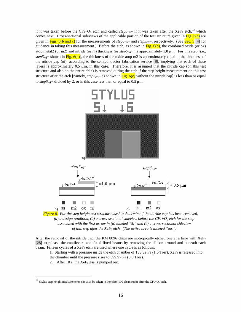
16

if it was taken before the CF4+O2 etch and called step5rA if it was taken after the XeF2 etch,12

which

comes next. Cross-sectional sideviews of the applicable portion of the test structure given in Fig. 6(a) are

given in Figs. 6(b and c) for the measurements of step5rA+ and step5rA, respectively. (See Sec. 5 [4] for

guidance in taking this measurement.) Before the etch, as shown in Fig. 6(b), the combined oxide (or ox)

atop metal2 (or m2) and nitride (or ni) thickness (or step5rA+) is approximately 1.0 m. For this step [i.e.,

step5rA+ shown in Fig. 6(b)], the thickness of the oxide atop m2 is approximately equal to the thickness of

the nitride cap (ni), according to the semiconductor fabrication service [8], implying that each of these

layers is approximately 0.5 m, in this case. Therefore, it is assumed that the nitride cap (on this test

structure and also on the entire chip) is removed during the etch if the step height measurement on this test

structure after the etch [namely, step5rA as shown in Fig. 6(c) without the nitride cap] is less than or equal

to step5rA+ divided by 2, or in this case less than or equal to 0.5 m.

a)

b) c)

Figure 6. For the step height test structure used to determine if the nitride cap has been removed,

(a) a design rendition, (b) a cross-sectional sideview before the CF4+O2 etch for the step

associated with the first arrow in (a) labeled “5,” and (c) a cross-sectional sideview

of this step after the XeF2 etch. (The active area is labeled “aa.”)

After the removal of the nitride cap, the RM 8096 chips are isotropically etched one at a time with XeF2

[28] to release the cantilevers and fixed-fixed beams by removing the silicon around and beneath each

beam. Fifteen cycles of a XeF2 etch are used where one cycle is as follows:

1. Starting with a pressure inside the etch chamber of 133.32 Pa (1.0 Torr), XeF2 is released into

the chamber until the pressure rises to 399.97 Pa (3.0 Torr).

2. After 10 s, the XeF2 gas is pumped out.

12

Stylus step height measurements can also be taken in the class 100 clean room after the CF4+O2 etch.

17

After a cursory microscopic inspection of the chips to ensure that the widest beams (present in the residual

strain and strain gradient groupings) are released, the chips are transported in a plastic container in a

zippered bag to a laboratory across campus where they are stored in a N2-filled dry box.

1.4.2 Post Processing of the RM 8097 Chips

For the RM 8097 chips processed in a surface-micromachined polysilicon multi-user MEMS process [9],

an additional backside etch is required to eliminate any stiction or squeeze film damping phenomena (see

Sec. 2.1 for details) associated with cantilever and fixed-fixed beam resonance frequency measurements.

An additional layer was added to the designs [as shown in Figs. YM3(a) and YM4(a) in Sec. 2.1] with

dimensions that represent the dimensions of the requested opening in the backside of the wafer. The

processing facility should be consulted for the appropriate design rules for this layer.

During the post processing, the front side of the wafer is protected, then the wafer thinned (removing the

backside films in the process) to a thickness similar to what is used in a silicon-on-insulator (SOI) multi-

user MEMS process [9]. Then, a backside photo patterning and RIE (reactive ion etch) are performed,

removing the silicon and stopping on the first oxide layer. [It stops on the first oxide layer because the

nitride layer, which is normally found between the 2 m sacrificial oxide layer and the Si wafer, is

patterned earlier in the process using a mask derived from the mask used to define the opening requested on

the backside of the wafer. Due to the patterning of this nitride layer, the edge of the nitride layer is

responsible for an approximate 600 nm vertical transition seen in the structural layer of suspended

cantilevers and fixed-fixed beams (as seen in Figs. YM3(b), YM4(b), and YM5 for a cantilever). There are

two such vertical transitions for fixed-fixed beams.]

An RIE etch is used due to its ability to create more vertical sidewalls (with a 10 angle) as opposed to the

(55 angle) sidewalls from a plasma etch. The RIE-etched sidewalls are sloped so that the digitized areas

representing the openings on the backside of the wafer are smaller than the desired openings on the front

side of the wafer.

After the backside etch, the exposed sacrificial oxides are etched, thereby releasing the beams. A super

critical CO2 dry is performed to minimize stiction for any beams that are designed with an underlying layer.

The chips are delivered to NIST with no protective coating, as requested. For delivery, they are typically

placed in a sealed clamshell package. Once the chips get to NIST, they are stored in a N2-filled dry box.

They are removed from the clamshell package before the expiration date of the adhesive, if applicable, then

inspected, as described in the following section.

1.5 Pre-Package Inspection

Before the RM 8096 and RM 8097 chips are packaged, they are inspected in a laboratory environment to

determine if they are suitable RM candidates. The RM 8097 chips are also inspected for classification

purposes. After the pre-package inspection and/or classification, the RM chips are returned to the N2-filled

dry box to await packaging.

1.5.1 Pre-Package Inspection of the RM 8096 Chips

The RM 8096 chips are inspected interferometrically (and/or microscopically) to ensure the following:

1. That there is at least one suitable test structure in the first, second, third, and fifth groupings of

test structures (namely, one cantilever in the Young’s modulus grouping, one fixed-fixed

beam in the residual strain grouping, one cantilever in the strain gradient grouping, and one

in-plane length test structure in the in-plane length grouping).

2. That there is at least one suitable step height test structure in the fourth grouping of test

structures for each of the four uniquely designed step height test structures. The resulting data

from these test structures in combination with data supplied by the semiconductor fabrication

18

service [8] can be used to obtain the thickness of the composite oxide beams, as given in Sec.

8, for the Young’s modulus measurements in Sec. 2.

3. That the chip is correctly classified, as specified in Sec. 1.3, as “acceptable.” Only

“acceptable” chips are RM 8096 candidates.

4. That the etched cavities have not merged. Although differences in color between a region that

is suspended and a region that is not suspended can be an indicator of non-merged cavities,

the existence of a flat region between the cavities (as verified upon examination of an

interferometric 2D data trace between the etched cavities) can be used as additional proof.

5. That the widest beams (located in the residual strain and strain gradient groupings) are

released. An interferometric 2D data trace (taken along the length of one of the cantilevers)

with data that curve out-of-plane can be used to verify that the widest beams are released.

6. That the etched cavity is deep enough so that squeeze film damping will not be an issue (see

Sec. 2.1 for details). This implies that the gap, d, between the bottom of the suspended

cantilever (for Young’s modulus measurements) and the top of the underlying layer is greater

than or equal to one-third the cantilever width [29].

The cantilevers for Young’s modulus measurements are all designed to be 28 m in

width. Therefore, d should be at least one-third that or 9.3 m. Since an isotropic XeF2

etch is used to release the beams and since the widest beam on the chip is 40m, this

implies that the lateral etch must traverse at least half this width (or 20m) in order for

the beams to release. Therefore, if the vertical etch rate is comparable to the lateral etch

rate, then the etched cavity, or dcav as shown in Fig. 7(c), should be at least 20 m. If we

assume here that d = dcav, which may be off by up to 0.5 m for flat beams,13

then 20 m

is much more than the minimum value of 9.3 m that is needed to ensure that squeeze

film damping will not be an issue.

As a double-check or if there is uncertainty about the vertical and lateral etch rates of

XeF2, interferometric measurements can be taken (both before the CF4+O2 etch and after

the XeF2 etch) from the fourth thickness test structure, as shown in Fig. 7(a), in the

Certification Plus grouping. In particular, an approximate step height measurement can

be taken for the step corresponding to either the 3rd

or 4th

arrow in this test structure. The

absolute value of the step height measurement taken before the CF4+O2 etch, as given by

the absolute value of step4DE+ or step4EF+ in Fig 7(b), is subtracted from the absolute

value of the step height measurement taken after the XeF2 etch, as given by the absolute

value of step4DE or step4EFin Fig. 7(c), to obtain an approximate measurement of the

depth of the cavity, dcav, as shown in Fig. 7(c).

7. That there are no stringers or debris present that would adversely affect the data taken on the

chosen test structures.

8. That sample static interferometric cantilever and fixed-fixed beam data can be taken on the

chosen beams used to obtain strain gradient and residual strain, respectively.

(a)

13

It should be noted that most, if not all, of the beams bend up.

19

(b) (c)

Figure 7. For the thickness test structure used to determine the depth of the etched cavity

(a) a design rendition, (b) a cross-sectional sideview before the CF4+O2 etch for the steps

associated with the third and fourth arrows in (a), and (c) a cross-sectional sideview

after the XeF2 etch for the steps associated with the third and fourth arrows in (a).

1.5.2 Pre-Package Inspection of the RM 8097 Chips

The RM 8097 chips are inspected interferometrically (and/or microscopically) to ensure the following:

1. That there is at least one suitable test structure in each of the five groupings of test structures

for the layer of interest (namely, if poly1 is the layer of interest, then one poly1 cantilever in

the Young’s modulus grouping, one poly1 fixed-fixed beam in the residual strain grouping,

one poly1 cantilever in the strain gradient grouping, one step height test structure in the step

height grouping, and one poly1 in-plane length test structure in the in-plane length grouping).

2. The existence of a suitable pegged cantilever (i.e., a cantilever exhibiting stiction) for the

layer of interest in the Certification Plus grouping of test structures under the label

“Thickness,” as seen in Figs. 2(a and b). (The resulting data from this test structure can be

used to obtain the poly1 or poly2 thickness, as given in Sec. 8, for Young’s modulus

measurements in Sec. 2.) In some cases, it may be preferable to obtain stiction data from a

test structure in the in-plane length grouping of test structures.

3. That useful static interferometric cantilever and fixed-fixed beam data can be taken on the

chosen poly1 or poly2 beams. For example, can residual strain and strain gradient data still

be taken on the beams if there is no curvature of the beams?

The layer of interest is determined for the given chip. Typically if the above criteria are satisfied for poly1

structures, the poly1 layer is considered the layer of interest unless, for example, the longest poly1

cantilevers do not bend out-of-plane, in which case the poly2 layer is considered the layer of interest

assuming the above criteria are met for poly2 structures.

1.5.3 Classification of the RM 8097 Chips

During the pre-package inspection of the RM 8097 chips, they are also classified as “acceptable” or

“unacceptable” using the following somewhat subjective criteria (as given below):

1. If one of the criteria in Sec. 1.5.2 is not satisfied for the layer of interest, the chip is classified

as “unacceptable,” and the following criteria can be overlooked.

2. If the anchor attachment point of most of the cantilevers and fixed-fixed beams in at least one

key array per grouping of test structures is intact and all or most of the beams are still present

in this key array, the chip is given an excellent or “acceptable” classification. [The poly1

arrays are considered key arrays if the poly1 parameters are reported on the RM Report of

Investigation as determined in Sec. 1.5.2. If the poly2 parameters are reported on the RM

20

Report of Investigation then the poly2 arrays are considered the key arrays. And, the same

applies to the arrays in the Young’s modulus grouping of test structures.]

3. If a portion of the anchor attachment point of most of the cantilevers and fixed-fixed beams in

at least one key array per grouping of test structures is missing due to an overetch from the

backside of the wafer, and all or most of the beams are still present in this key array, the

classification may be either “acceptable” or “unacceptable.”

4. As a rule of thumb, as less of the anchor attachment point remains intact and as the number of

beams in the key arrays decreases, the classification degrades from “acceptable” to

“unacceptable.”

The dividing line between the classification categories can be somewhat subjective, so to help ensure

consistency with respect to the same criteria, all of the chips received are inspected and classified during

the same data session and by the same person.

1.6 Packaging

After an RM 8096 or RM 8097 chip passes the post processing inspection, it is packaged as shown in Fig.

8; however, the piezoelectric transducer (PZT) wires may be connected to different pins. The chips are

packaged in a laboratory environment in the following way:

1. The hybrid package has a pin arrangement similar to that shown in Fig. 8(a) with a 1 mm pin-

to-pin separation. The package is 20.32 mm wide, 27.94 mm long, and 19.05 mm tall (with

the lid on and including the height of the exposed pins on the bottom of the package). The

height of the exposed pins on the bottom of the package is 5.08 mm.

2. The PZT is secured to the top of the chip cavity using two thin layers of low stress, non-

conducting epoxy (Ellsworth Adhesives Resinlab UR 3010 Clear Urethane Encapsulant).

(The first layer of epoxy ensures that there will not be a conducting path between the package

and the PZT.)

3. The PZT has the following properties:

a. The operating voltage range is from 20 V to +120 V.

b. The maximum operating temperature is 150 ºC.

c. The dimensions of the PZT are approximately 5 mm by 5 mm and 2 mm in height.

d. It is provided with a red and a black wire. The red wire should be driven with a

voltage that is positive relative to the black wire.

e. It can achieve a 2.2 m (±20 %) displacement at 100 V from DC to 100 kHz.

f. It has an electrical capacitance of 250 nF (±20 %).

g. It has a resonance frequency greater than 300 kHz, at which or above which it shall

not be operated because that could damage the PZT.

4. Each PZT wire is soldered to the upper portion of a package pin to ensure that it is connected

and to avoid any arcing.

5. The PZT is activated at 10 V and 7000 Hz to ensure that the resulting PZT vibration is barely

audible and properly connected. (Alternatively, the PZT can be checked with a vibrometer to

ensure that the vibration is audible for a periodic chirp function between 5 kHz and 20 kHz.)

6. The RM chips are secured to the top of the PZT.

a. The RM 8096 chips are secured using two thin layers of a low stress non-

conducting epoxy. (The first layer of epoxy ensures that there will not be a

conducting path between the PZT and the RM.)

b. For the RM 8097 chips, one layer of the low stress non-conducting epoxy is allowed

to dry on top of the PZT. Then, a thin layer of this epoxy is spread on top of the

bottom half of the existing epoxy so that only the bottom half of the RM 8097 chip

when placed on top of it will be secured to the PZT. Then, the bottom half of the

RM 8097 chip is placed atop this thin layer of epoxy so that none of it seeps through

the portions of the chip that were etched from the backside.

7. The lid (or can) is placed on top of the package to protect the chip and the lid is secured to

the package (with a plastic chip, tape, or by another means) before shipment.

The packaged chips are stored in a N2-filled dry box.

21

(a)

(b)

Figure 8. For the MEMS 5-in-1 (a) a drawing of the packaged chip and (b) a photograph of one of the

chips inside the package cavity

1.7 NIST Measurements on the MEMS 5-in-1

NIST measurements are taken on the packaged RMs in a laboratory environment. The chosen test

structures are identified and the measurements are taken following the procedures in the applicable

standard test method [1-5]. (See also Sec. 2 through Sec. 8, inclusive, for overall guidance.) The data are

entered into the pertinent data analysis sheet [13] in order to perform the calculations and verify the data.

After verification of the data, the resulting calculated values are entered on the appropriate RM 8096 or RM

8097 Report of Investigation.

22

1.8 The RM Report of Investigation

The RM Report of Investigation may evolve over time. For a current example of the RM 8096 and 8097

Report of Investigation, see the Data and Information Files link on https://www-

s.nist.gov/srmors/view_detail.cfm?srm=8096 and https://www-

s.nist.gov/srmors/view_detail.cfm?srm=8097, respectively. Both of these Reports of Investigation as of the

writing of this SP 260 include the following: 1. The DOC logo,

2. A serial number for the individually tested RM,

3. NIST reference values and uncertainties for Young’s modulus, residual strain, strain gradient,

step height, in-plane length, residual stress, stress gradient, and thickness,

4. The issue date,

5. The expiration date,

6. An overview,

7. A brief description of the MEMS 5-in-1,

8. Instructions for use,

9. Material available for the MEMS 5-in-1, and

10. References.

1.9 Traceability

Measurements made using the MEMS 5-in-1 achieve traceability to the NIST measurements on the RM.

This constitutes traceability to a national standard, but, in general, traceability to the International System

of Units [17,18] cannot be claimed.

At some point, if it is deemed appropriate that the MEMS 5-in-1 RM become an SRM, there are already

certain elements of traceability to the SI that are already in place or that can easily be implemented; for

example, NIST traceable measurements to the SI in the x-, y-, and z-directions as well as for frequency

measurements.

For measurements in the z-direction, measurement data from the optical interferometer and the stylus

profilometer are calibrated from data taken on a certified physical step height standard as specified in Sec.

5.2. The instrument calibration is also checked with the certified value of a second physical step height

standard (as detailed in Sec. 1.1.2.2). These commercial physical step height standards are calibrated

directly at NIST. Therefore, the measurements in the z-direction for the MEMS 5-in-1 are NIST-traceable

measurements.

For measurements in the x- and y-directions, the optical interferometer is calibrated as specified in Sec. 6.2

using either the 2.5 mm ruler (with a 4.0 µm pitch) that is located in the Certification Plus group of test

structures on an RM 8097 chip or it is calibrated with a 10 mm stage micrometer (with a 10.0 µm pitch)

that has a calibration certificate with NIST-traceable measurements. Therefore, the measurements taken in

the x- and y-direction for the MEMS 5-in-1 provide either NIST-traceable measurements or easy to

implement NIST-traceable measurements.

For frequency measurements, before each data session, the maximum frequency of the optical vibrometer

and the stroboscopic interferometer is measured with a 10-digit/s frequency counter that has been calibrated

by the vendor to provide NIST-traceable measurements. A calibration factor, calf, is determined as

specified in Sec. 2.2. From this maximum frequency, all other signals are derived and the frequency

measurements are multiplied by calf to obtain calibrated values. As specified in Sec. 1.1.1.2, the instrument

calibration is also checked by comparing one or more resonance frequency measurements (via Young’s

modulus calculations) a) with previous resonance frequency measurements (or Young’s modulus

calculations) using the same cantilevers and/or b) with resonance frequency measurements (or Young’s

modulus calculations) obtained from another calibrated instrument using the same resonating cantilevers.

Therefore, the measured resonance frequency for the MEMS 5-in-1 is a NIST-traceable measurement.

https://www-s.nist.gov/srmors/view_detail.cfm?srm=8096




23

The traceability chain for the physical step heights, the stage micrometer, as well as the traceability chain

for the certification of frequency can be obtained by sending an email request to [email protected].

1.10 Material Available for the MEMS 5-in-1

After you order a MEMS 5-in-1, you will receive a packaged RM chip, a Report of Investigation,

completed data analysis sheets, a copy of each of the standard test methods [1-5], and this SP 260. Besides

this SP 260, one of the best places from which to obtain information associated with the MEMS 5-in-1 is

the MEMS Calculator Website [13]. The symbol is used on this website to help you quickly find

material associated with the MEMS 5-in-1. From this website you can obtain the following:

1. This SP 260,

2. An overview article for the MEMS 5-in-1 [15],

3. The data analysis sheets (e.g., YM.3, RS.3, SG.3, SH.1.a, L.0, T.1, and T.3.a),

4. Sample data traces for residual strain, strain gradient, step height, and in-plane length,

5. Ordering information for a MEMS 5-in-1,

6. The design file and an accompanying tiff file of each MEMS 5-in-1 chip,

7. The list of the following two SEMI standard test methods [1,4] and three ASTM standard test

methods [2-3,5] along with links for ordering information:

SEMI standard test method MS4, Test Method for Young’s Modulus Measurements of

Thin, Reflecting Films Based on the Frequency of Beams in Resonance,

ASTM standard test method E 2245, Test Method for Residual Strain Measurements of

Thin, Reflecting Films Using an Optical Interferometer,

ASTM standard test method E 2246, Test Method for Strain Gradient Measurements of

Thin, Reflecting Films Using an Optical Interferometer,

SEMI standard test method MS2, Test Method for Step Height Measurements of Thin

Films, and

ASTM standard test method E 2244, Test Method for In-Plane Length Measurements of

Thin, Reflecting Films Using an Optical Interferometer, and

8. Pertinent references (for downloading from the website) grouped below by topic area:

Young’s modulus, step height, and thickness [10,30],

Step height and thickness [6,7], and

Residual strain, strain gradient, and in-plane length [11,14].

This SP 260 focuses on how to use the MEMS 5-in-1 to successfully take measurements with

the standard test methods. The above-mentioned references were stepping stones in creating

this guide. The references are more general in nature, contain more background information,

and provide for more applications of the various test methods.

In addition, during the course of this work, an assessment was performed, as given below,

which specifies the importance of standardization efforts and can be used to guide future

standardization efforts:

An assessment of the US Measurement System [31].

The appropriate standard test method is used to guide you through the measurements. If you have

difficulties understanding the technical basis for the steps in the standard test methods, you can consult this

SP 260 or one of the pertinent references [6-7,10-11,14,30-31], which can be downloaded from the website.

1.11 Storage and Handling

The packaged RM is labeled, placed in a small foam-padded wooden box for protection, and delivered

along with the Report of Investigation, the data analysis sheets, the five standard test methods [1-5], and

this SP 260 to NIST’s Building 301 where it is also labeled, then sealed in a plastic bag and stored in a N2-

filled dry box (or an acceptable alternative) to await shipment to a customer.

The semiconductor test chip is subject to surface contamination and oxidation during storage and handling.

The RM should be handled using the metal package, without contacting the semiconductor test chip. The

mailto:[email protected]

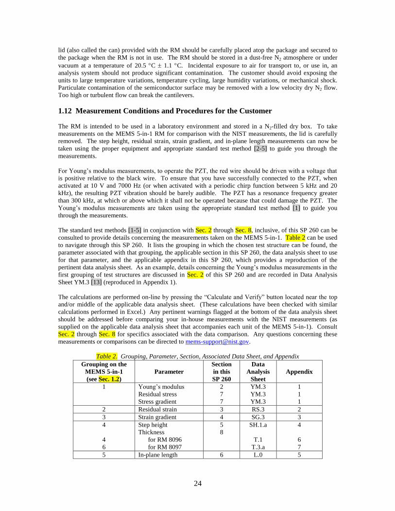
24

lid (also called the can) provided with the RM should be carefully placed atop the package and secured to

the package when the RM is not in use. The RM should be stored in a dust-free N2 atmosphere or under

vacuum at a temperature of 20.5 C 1.1 C. Incidental exposure to air for transport to, or use in, an

analysis system should not produce significant contamination. The customer should avoid exposing the

units to large temperature variations, temperature cycling, large humidity variations, or mechanical shock.

Particulate contamination of the semiconductor surface may be removed with a low velocity dry N2 flow.

Too high or turbulent flow can break the cantilevers.

1.12 Measurement Conditions and Procedures for the Customer

The RM is intended to be used in a laboratory environment and stored in a N2-filled dry box. To take

measurements on the MEMS 5-in-1 RM for comparison with the NIST measurements, the lid is carefully

removed. The step height, residual strain, strain gradient, and in-plane length measurements can now be

taken using the proper equipment and appropriate standard test method [2-5] to guide you through the

measurements.

For Young’s modulus measurements, to operate the PZT, the red wire should be driven with a voltage that

is positive relative to the black wire. To ensure that you have successfully connected to the PZT, when

activated at 10 V and 7000 Hz (or when activated with a periodic chirp function between 5 kHz and 20

kHz), the resulting PZT vibration should be barely audible. The PZT has a resonance frequency greater

than 300 kHz, at which or above which it shall not be operated because that could damage the PZT. The

Young’s modulus measurements are taken using the appropriate standard test method [1] to guide you

through the measurements.

The standard test methods [1-5] in conjunction with Sec. 2 through Sec. 8, inclusive, of this SP 260 can be

consulted to provide details concerning the measurements taken on the MEMS 5-in-1. Table 2 can be used

to navigate through this SP 260. It lists the grouping in which the chosen test structure can be found, the

parameter associated with that grouping, the applicable section in this SP 260, the data analysis sheet to use

for that parameter, and the applicable appendix in this SP 260, which provides a reproduction of the

pertinent data analysis sheet. As an example, details concerning the Young’s modulus measurements in the

first grouping of test structures are discussed in Sec. 2 of this SP 260 and are recorded in Data Analysis

Sheet YM.3 [13] (reproduced in Appendix 1).

The calculations are performed on-line by pressing the “Calculate and Verify” button located near the top

and/or middle of the applicable data analysis sheet. (These calculations have been checked with similar

calculations performed in Excel.) Any pertinent warnings flagged at the bottom of the data analysis sheet

should be addressed before comparing your in-house measurements with the NIST measurements (as

supplied on the applicable data analysis sheet that accompanies each unit of the MEMS 5-in-1). Consult

Sec. 2 through Sec. 8 for specifics associated with the data comparison. Any questions concerning these

measurements or comparisons can be directed to [email protected].

Table 2. Grouping, Parameter, Section, Associated Data Sheet, and Appendix

Grouping on the

MEMS 5-in-1

(see Sec. 1.2)

Parameter

Section

in this

SP 260

Data

Analysis

Sheet

Appendix

1 Young’s modulus

Residual stress

Stress gradient

2

7

7

YM.3

YM.3

YM.3

1

1

1

2 Residual strain 3 RS.3 2

3 Strain gradient 4 SG.3 3

4

4

6

Step height

Thickness

for RM 8096

for RM 8097

5

8

SH.1.a

T.1

T.3.a

4

6

7

5 In-plane length 6 L.0 5


25

1.13 Homogeneity of the RMs

The MEMS 5-in-1 chips are given an RM number based upon where it is fabricated. (The RM 8096 chips

are fabricated on a multi-user 1.5 µm CMOS process followed by a bulk-micromachining etch. The RM

8097 chips are fabricated using a polysilicon multi-user surface-micromachining MEMS process with a

backside etch.) The multi-user portion of these processes is well known in the community such that

customers are willing to purchase chips on these processing runs due to the known homogeneity of the

parts received, which makes them reliable. Therefore, by definition, the RMs are associated with

homogeneous processes.

For RM 8096, the chips are initially classified as given in Sec. 1.3 after they are received from the

fabrication service. The post-processing is performed at NIST on one chip at a time (as specified in Sec.

1.4.1) in order to obtain the most reliable results. Initially, a CF4+O2 etch is used to remove the nitride cap

present atop the chips when they are received from the fabrication service. Measurements are taken to

determine if the nitride cap has been removed. Then, a XeF2 etch removes any exposed silicon next to and

beneath a composite oxide beam in order to release it. The chips are inspected as given in Sec. 1.5.1 and it

is verified that they are correctly classified as “acceptable” or “unacceptable” for use as an RM. Thickness

(a parameter that can be affected by an etch) is one of the parameters with an uncertainty that is reported on

the Report of Investigation. Also, effective values are reported for the material parameters due to

deviations from the ideal geometry and composition of the test structures.

The back-side etch for RM 8097 is performed at MEMSCAP as specified in Sec. 1.4.2. This additional

etch is performed while the two polysilicon layers (one of which is used for the measurements taken on RM

8097) are completely covered with a sacrificial oxide. Therefore, this back-side etch does not affect the

homogeneity of the parts measured. In addition, when the RM 8097 chips are received from the fabrication

facility, they are inspected and classified as “acceptable” or “unacceptable” as given in Sec. 1.5.2 and 1.5.3,

respectively.

1.14 Stability Tests

For stability tests, one packaged part is stored in a N2-filled dry box and one packaged part is stored in a

plastic storage container. These two packaged parts are called RM monitors. When the MEMS 5-in-1

chips are measured, so are the RM monitors from the same processing run, and the same measurements are

taken. A parametric value resulting from the first measurements taken on the RM monitors is called R; its

combined standard uncertainty value is called uR.

Tables 3 and 4 give the correction terms and specific standard deviations that are typically used at NIST in

the applicable data analysis sheets for certain parameters on RM 8096 and RM 8097. Similar quantities are

not used in all the data analysis sheets. For example, a relative repeatability standard deviation,

σrepeat(samp) for Young’s modulus is not provided in Tables 3 and 4 because a repeatability component is

not needed in its uncertainty equation because the propagation of uncertainty technique [21-23] (a brief

overview of which is given in Appendix 8) is used to obtain this uncertainty equation and including this

repeatability component would be double counting uncertainties. This is the case for residual stress and

stress gradient as well. In addition, thickness values are obtained from step height measurements, and since

the step height uncertainty results (which already include a repeatability component) will be utilized in the

thickness uncertainty calculations, a repeatability standard deviation is not needed for thickness. It should

be pointed out that σrepeat(samp) is a relative repeatability standard deviation and σrepeat(samp)’, which has a

trailing “΄” in the subscript, is an absolute repeatability standard deviation which is used for the in-plane

length measurements.

Stability tests can be used to track parametric changes as a function of, for example, time and temperature.

For the MEMS 5-in-1, the Report of Investigation states rigid temperature requirements (i.e., 20.5 C 1.1

C) within which the parameters are not expected to significantly change. Therefore, for the MEMS 5-in-1,

only variations as a function of time are tracked for the RM monitor stored in a plastic storage container

and the RM monitor stored in a N2-filled dry box. And, given the domino effect discussed in the next

26

section, only the residual strain needs to be monitored quarterly. This measurement is performed on the

same RM monitor test structures that are used to obtain the reference values for that chip. A parametric

value resulting from a measurement taken on a quarterly basis is considered a measured value, M, with its

combined standard uncertainty value, uM.

Table 3. Correction Terms and Specific Standard Deviations Typically Used at NIST for RM 8096

Parameter Correction

Terma

Standard

Deviationa

Values used

with

RM 8096

1. Young’s modulus L = 200 µm fcorrection

σsupport

σcantilever

2.67 kHz

0.63 kHzb

0.63 kHzb

L = 300 µm fcorrection

σsupport

σcantilever

0 kHz

0 kHz

0 kHz


σsupport

σcantilever

–0.240 kHz

0.057 kHzb

0.057 kHzb

2. Residual strain at 25× δεrcorrection 0

at 25× σrepeat(samp) 2.49 %

Loffset

(RM 8097,

p0-to-p0 at 25×)

0.129 µm

σLrepeat(samp)’c

(RM 8097,

p0-to-p0 at 25×)

0.213 µm

3. Strain gradient L = 200 µm (at 25×) sgcorrection 0 m

–1 d

L = 248 µm (at 25×) sgcorrection 0 m

–1 d

at 25× σrepeat(samp) 3.02 %

4. Step height at 25× σrepeat(samp) 3.95 %

5. In-plane length

(for edges that

face each other)

L = 200 µm

(m2-to-m2 at 25×) Loffset 2.63 µm

L = 200 µm

(m2-to-m2 at 25×)

σrepeat(samp)΄c 1.16 µm

6. Rtave = Rt

(peak-to-valley)

along top of m2 in

in-plane length

group (at 25×)

119.5 nm

7. Rave = Ra

(surface roughness)

along top of m2 in

in-plane length

group (at 25×)

17.3 nm

a Consult the pertinent section in this SP 260 for details associated with these correction terms and specific standard

deviations. b Where support =cantilever= |fcorrection | / [3 SQRT(2)].

c The trailing prime in this subscript implies an absolute measurement.

d This is an assumption since it is difficult to obtain data points beyond 250 µm along the length of the cantilever due to

excessive curvature of the cantilever.

27

Each quarter, the positive difference, D, between the first measured or reference value, R, and that quarter’s

measured value, M, of residual strain is calculated along with the uncertainty of the difference, uD, using

the following equations:

RMD , and (29)

22

RMD uuu . (30)

Table 4. Correction Terms and Specific Standard Deviations Typically Used at NIST for RM 8097


Terma

Standard

Deviationa

Values used

with RM

8097

1. Young’s modulus

P1:


σsupport

σcantilever

1.095 kHz

0.258 kHzb

0.258 kHzb

P2:


σsupport

σcantilever

0.860 kHz

0.203 kHzb

0.203 kHzb

P1:


σsupport

σcantilever

0 kHz

0 kHz

0 kHz

P2:


σsupport

σcantilever

0 kHz

0 kHz

0 kHz

P1:


σsupport

σcantilever

0.122 kHz

0.029 kHzb

0.029 kHzb

P2:


σsupport

σcantilever

0.0208 kHz

0.0049 kHzb

0.0049 kHzb

2. Residual strain P1 at 5×: δεrcorrection

σrepeat(samp)

0

5.5 %

Loffset

σLrepeat(samp)’c

3.69 µm

0.00 µm

P2 at 5×: δεrcorrection

σrepeat(samp)

0

3.7 %

Loffset

σLrepeat(samp)’c

1.38 µm

0.64 µm

a Consult the pertinent section in this SP 260 for details associated with these correction terms and specific standard

deviations. b Where support =cantilever= |fcorrection | / [3 SQRT(2)].

c The trailing prime in this subscript implies an absolute measurement.

28

Table 4, Continued. Correction Terms and Specific Standard Deviations Typically Used at NIST for RM 8097


Terma

Standard

Deviationa

Values used

with RM 8097

3. Strain gradient

P1 at 5×:

L = 400 µm sgcorrection

0.65 m

–1

P1 at 5×:

L = 450 µm sgcorrection 0.00 m

–1

P1 at 5×:


0.65 m

–1

P1 at 5×:


–1

P1 at 5×:


σrepeat(samp)

1.94 m–1

12.5 %

P1 at 5×:


–1

P1 at 5×:


3.23 m–1

P1 at 5×:


–1

P1 at 5×:


4.52 m–1

P2 at 5×:


1.00 m

–1

P2 at 5×:


–1

P2 at 5×:


1.00 m

–1

P2 at 5×:


–1

P2 at 5×:


σrepeat(samp)

3.00 m–1

13.4 %

P2 at 5×:


–1

P2 at 5×:


5.00 m

–1

P2 at 5×:


–1

P2 at 5×:


7.00 m

–1

4. Step height at 20× σrepeat(samp) 7.35 %

5. In-plane length

(for edges that

face each

other)

L = 1000 µm

(p1-to-p1 at 5×) Loffset=LdesLalignave

σrepeat(samp)΄b

3.69 µm

0.00 µm

L = 1000 µm

(p2-to-p2 at 5×) Loffset=LdesLalignave

σrepeat(samp)΄b

1.38 µm

0.64 µm

6. Rtave =Rt

(peak-to-valley)

P0 at 5×: 28.12 nm

P1 at 5×: 17.38 nm

P2 at 5×: 16.79 nm

7. Rave = Ra

(surface roughness)

P0 at 5×: 4.87 nm

P1 at 5×: 2.97 nm

P2 at 5×: 3.03 nm a Consult the pertinent section in this SP 260 for details associated with these correction terms and specific standard

deviations. b The trailing prime in this subscript implies an absolute measurement.

29

For the RM monitor stored in a plastic storage container, if the following equation is not satisfied:

DuD 2 , (31)

the residual strain begins to be monitored monthly. Once Eq. (31) is not satisfied for the RM monitor

stored in a N2-filled dry box, the material parameters can be considered out of calibration and the customers

in possession of those RMs from the same processing run are notified, assuming their RM Report of

Investigation has not already expired (as discussed in the next section).

1.15 Length of Certification

It is recommended that the customer purchase a MEMS 5-in-1 RM every two years. For a chip processed

similarly to RM 8097 and stored in a plastic storage container (not a N2-filled dry box), residual strain data

taken on this chip between May 2002 and August 2005, as shown in Fig. 9, indicate that the residual strain

increases as a function of time.14

Therefore, at the very least for the MEMS 5-in-1 RM 8097, this parameter

should be periodically checked at NIST. As a safeguard, it should also be periodically checked for RM

8096.

In Fig. 9, the data are smoothed out by connecting the second and fourth data points. Let us assume that

the first data point is called R, with combined standard uncertainty uR, and expanded uncertainty [21-23]

UR, where UR=kuR=2uR (with k=2 to approximate a 95 % level of confidence). As an approximation for the

maximum separation between parametric values, let us assume that the third data point corresponds to M,

as defined in Sec. 1.14, with combined standard uncertainty uM, and expanded uncertainty UM, where

UM=kuM=2uM (with k=2 to approximate a 95 % level of confidence). The value for D is then calculated

using Eq. (29) and UD is calculated using the following equation:

222 RMD uuU . (32)

Then, the horizontal dotted line is plotted in Fig. 9, which corresponds to R plus UD. This dotted line

intersects the dotted line corresponding to the smoothed out data. The time between this intersection point

and the measurement of R is slightly more than two years. Therefore, purchasing a MEMS 5-in-1 RM

every two years is recommended to ensure that D<UD for residual strain.

In addition, if the residual strain is out of calibration, it implies that the residual stress may also be out of

calibration (since the residual strain is used to calculate residual stress). This domino effect continues for

the remaining material parameters, as indicated in Table 5. Therefore, to ensure the calibration of the five

material parameters (Young’s modulus, residual strain, strain gradient, residual stress, and stress gradient)

it is recommended that a MEMS 5-in-1 RM be purchased every two years. Since only one date can be

supplied on the RM Report of Investigation indicating the length of certification, for all the 5-in-1

parameters, it is recommended that a MEMS 5-in-1 RM be purchased every two years. This will allow for

improvements in equipment and procedures for the three dimensional parameters (step height, in-plane

length, and thickness) which are not expected to change as a function of time.

14

The reason for this increase is not known.

30

Figure 9. Residual strain data as a function of time for a surface micromachined chip where the

uncertainty bars correspond to 12.0 % to represent the estimated expanded uncertainty values.

The chip was stored in a plastic storage container.

Note: In this figure, the uncertainty bars are calculated using U = 2[ucave2 + σrepeat(samp)

2]1/2

with ucave=1.8 % as given in [11] and σrepeat(samp)=5.70 % as derived from data given in [11].

Table 5. Length of Certification for the MEMS 5-in-1 Parameters

Parameter

Length of

Certification

Reason for Expiration of Calibration

1. residual strain two years in case the residual strain varies as a function of time (see Fig. 9)

2. residual stress two years residual strain is used to calculate residual stress

3. Young’s modulus two years Young’s modulus is used to calculate residual stress

(even though this parameter is not expected to vary as a function

of time, its value may be questioned if the chip experienced

unexpected environmental variations)

4. stress gradient two years Young’s modulus is used to calculate stress gradient

5. strain gradient two years strain gradient is used to calculate stress gradient

(even though Fig. 10 indicates that this parameter is not expected

to vary as a function of time, since the value of the other material

parameters may be in question, this one may be as well if the

chip experienced environmental variations not experienced by

the chips from which the data were taken in Fig. 10)

6. step height two years to allow for improvements in equipment and procedures

7. thickness two years to allow for improvements in equipment and procedures

8. in-plane length two years to allow for improvements in equipment and procedures

31

Strain Gradient Data

May 2002 to March 2004

0

2

4

6

8

Nov-01 May-02 Dec-02 Jun-03 Jan-04 Aug-04

Month

sg (

m

1)

Figure 10. Strain gradient round robin data as a function of time for lengths ranging

from 500 m to 650 m. The chip was stored in a plastic storage container.

Recalibration of the MEMS 5-in-1 RM is not recommended (and also currently not offered at NIST) for the

following reasons:

1. Improvements inevitable: Improvements in device design, processing, equipment and

procedures are inevitable. Maintaining an “out-of-date” RM would not be keeping up with

the current state of technology.

2. Price: Since the fabrication costs of the MEMS 5-in-1 chips are supplied free of charge by

the fabrication service for RM 8096 [8] and supplied either free of charge or cost shared by

the fabrication facility for RM 8097 [9], the cost to recalibrate a MEMS 5-in-1 RM is almost

comparable to the purchase price of a new MEMS 5-in-1 RM. In other words, the cost for

both mainly revolves around the cost to measure the parameters on the chips.

3. Degrading quality: With continued use in air, the pertinent test structures on the RMs are

bound to get dirty.

4. Turn-around time: It is more desirable to be in a position of offering RMs when they are

available as opposed to the challenge of getting an RM recalibrated within a reasonable

amount of time which would require that:

a. The step height standards and frequency meter are in calibration,

b. The instrumentation has been maintained, is operational, and in calibration,

c. The personnel are available to perform the recalibrations,

d. The RM is not inadvertently mishandled, and

e. Nothing goes wrong.

In other words, it is easier to guarantee a more reasonable turn-around time by not offering

recalibrations.

5. Lack of efficiency and cost-effectiveness: Providing calibration services requires equipment

devoted solely to that service, which would be an added expense, not only for the equipment

and space, but also in terms of personnel, overhead, and time. The alternative of providing

the RMs (without recalibrations) enables the equipment and space to be shared. This is a

more efficient, cost-effective approach.

Thus, it is recommended that a MEMS 5-in-1 RM be purchased every two years. The customer should

contact the SRM Program Office for specifics.

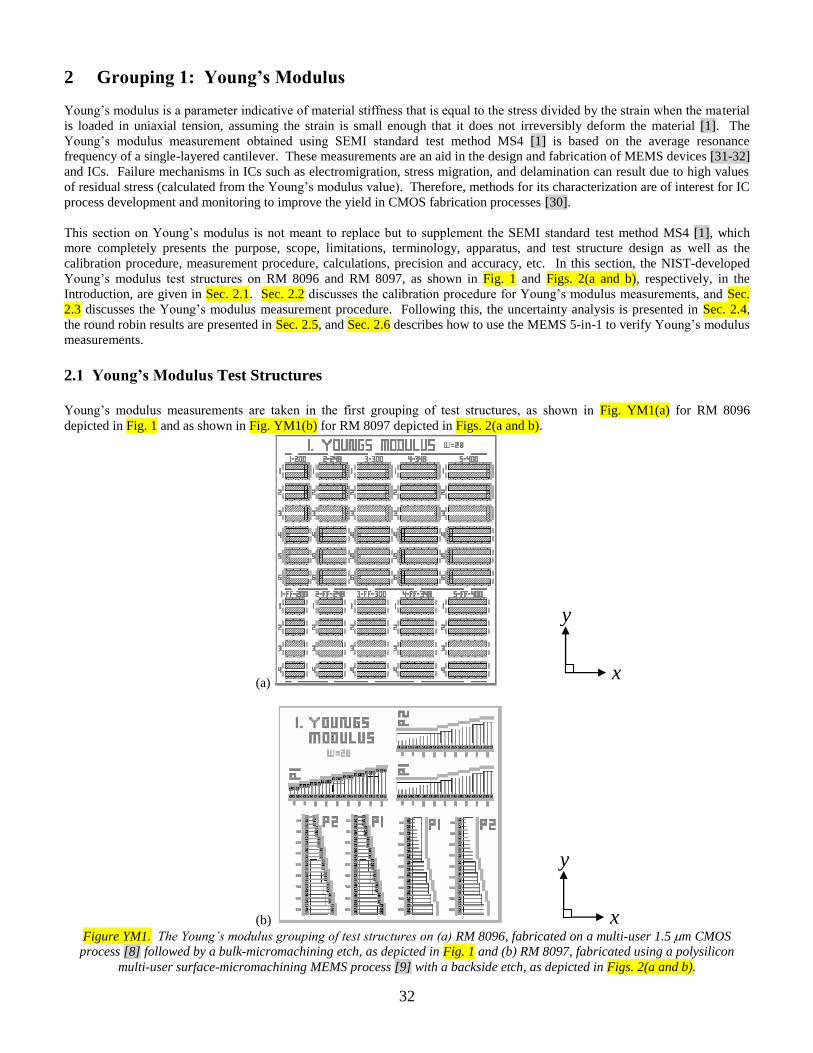
32

2 Grouping 1: Young’s Modulus

Young’s modulus is a parameter indicative of material stiffness that is equal to the stress divided by the strain when the material

is loaded in uniaxial tension, assuming the strain is small enough that it does not irreversibly deform the material [1]. The

Young’s modulus measurement obtained using SEMI standard test method MS4 [1] is based on the average resonance

frequency of a single-layered cantilever. These measurements are an aid in the design and fabrication of MEMS devices [31-32]

and ICs. Failure mechanisms in ICs such as electromigration, stress migration, and delamination can result due to high values

of residual stress (calculated from the Young’s modulus value). Therefore, methods for its characterization are of interest for IC

process development and monitoring to improve the yield in CMOS fabrication processes [30].

This section on Young’s modulus is not meant to replace but to supplement the SEMI standard test method MS4 [1], which

more completely presents the purpose, scope, limitations, terminology, apparatus, and test structure design as well as the

calibration procedure, measurement procedure, calculations, precision and accuracy, etc. In this section, the NIST-developed

Young’s modulus test structures on RM 8096 and RM 8097, as shown in Fig. 1 and Figs. 2(a and b), respectively, in the

Introduction, are given in Sec. 2.1. Sec. 2.2 discusses the calibration procedure for Young’s modulus measurements, and Sec.

2.3 discusses the Young’s modulus measurement procedure. Following this, the uncertainty analysis is presented in Sec. 2.4,

the round robin results are presented in Sec. 2.5, and Sec. 2.6 describes how to use the MEMS 5-in-1 to verify Young’s modulus

measurements.

2.1 Young’s Modulus Test Structures

Young’s modulus measurements are taken in the first grouping of test structures, as shown in Fig. YM1(a) for RM 8096

depicted in Fig. 1 and as shown in Fig. YM1(b) for RM 8097 depicted in Figs. 2(a and b).

(a)

(b)

Figure YM1. The Young’s modulus grouping of test structures on (a) RM 8096, fabricated on a multi-user 1.5 m CMOS

process [8] followed by a bulk-micromachining etch, as depicted in Fig. 1 and (b) RM 8097, fabricated using a polysilicon

multi-user surface-micromachining MEMS process [9] with a backside etch, as depicted in Figs. 2(a and b).

y

x

y

x

33

The Young’s modulus is obtained from resonance frequency measurements of a cantilever. A design rendition of a cantilever

test structure in the Young’s modulus grouping of test structures, as shown in Figs. YM1(a and b), can be seen respectively in

Fig. YM2(a) for the bulk-micromachined RM 8096 chip and in Figs. YM3(a) and YM4(a) for the surface-micromachined RM

8097 chip with a backside etch for a poly1 (or p1) cantilever and a poly2 (or p2) cantilever, respectively. Cross sections of these

test structures can be seen in Figs. YM2(b and c), Figs. YM3(b and c), and Figs. YM4(b and c), respectively.

(a)

(b)

(c)

Figure YM2. For a cantilever test structure on a bulk-micromachined RM 8096 chip shown in Fig. 1

(a) a design rendition, (b) a cross section along Trace a in (a), and (c) a cross section along Trace b in (a).

y

x

metal2 (m2)

dimensional

marker

exposed silicon

to be etched

(design layers

include active

area, contact,

via, and glass) etch stop

(n-implant

encompassing

active area) 16 m

a

b

34

(a)

(b)

(c)

Figure YM3. For a p1 cantilever test structure on a surface-micromachined RM 8097 chip (with a backside etch) shown

in Figs. 2(a and b) (a) a design rendition, (b) a cross section along Trace a in (a), and (c) a cross section along Trace b in (a).

35

(a)

(b)

(c)

Figure YM4. For a p2 cantilever test structure on a surface-micromachined RM 8097 chip (with a backside etch) shown

in Figs. 2(a and b) (a) a design rendition, (b) a cross section along Trace a in (a), and (c) a cross section along Trace b in (a).

36

The specifications for the cantilevers shown in Figs. YM1(a and b) for RM 8096 and RM 8097, respectively, are given in Table

YM1.

Table YM1. Cantilever Specifications for Young’s Modulus Measurements

For RM 8096 For RM 8097

Structural Layer SiO2 poly1 poly2

Wcan (m) 28 20 20

Lcan (m) 200, 248, 300, 348, and 400 100, 150, 200, 250, 300, 350,

400, 450, and 500

100, 150, 200, 250, 300, 350,

400, 450, and 500

t (m) 2.743 2.0 1.5

Orientationa 0 and 180 0 and 90 0 and 90

Quantity of Beams three of each length and for each

orientation (making 30 beams)

three of each length and for

each orientation (making 54

beams)

three of each length and for

each orientation (making 54

beams)

Einit (GPa) 70 160 160

(g/cm3) 2.2 2.33 2.33

aA 0 orientation implies that the length of the beam is parallel to the x-axis of the test chip, the axes of which are shown

in Fig. 1 and again in Fig. YM2 for RM 8096 [and in Figs. 2(a and b) and again in Figs. YM3 and YM4 for RM 8097], with

the connection point of the cantilever having a smaller x-value than the x-values associated with the suspended portion

of the cantilever.

For RM 8096: On RM 8096, all oxide cantilevers shown in Fig. YM1(a) are designed with both a 0 orientation and a 180

orientation. As seen in this figure, the length of a cantilever (in micrometers) is given at the top of each column of cantilevers

following the column number (i.e., 1 to 5). These design lengths (and the design width) are specified in Table YM1. There are

three cantilevers designed at each length for each orientation. Therefore, there are 15 oxide cantilevers with a 0 orientation and

15 oxide cantilevers with a 180 orientation. The fixed-fixed beams shown in the bottom portion of the Young’s modulus

grouping of test structures shown in Fig. YM1(a) will not be used for RM measurements.

As specified in Sec. 1.4.1 for RM 8096, the exposed silicon, as shown in Fig. YM2(a), is isotropically etched in XeF2 to release

the cantilever, as shown in Fig. YM2(b), by removing the silicon around and beneath the cantilever. The dimensional markers

are instrumental in firming up the support region. They also can be used to measure the small amount of SiO2 that has also been

etched in XeF2,15

however the tip of the cantilever will also be etched a comparable amount so that the length of the cantilever

should remain the same. The etch stop, also shown in this figure, helps to inhibit the etch away from the test structure to shield

neighboring structures from the etch. It consists of an n-implant designed to surround the active area. As seen in Fig. YM2(c),

there is undercutting of the beam.

For RM 8096, the dimensions were chosen such that 5 m < Wcan < 40 m, Wcan > t, and Lcan >> t where t=2.743 m, as

determined by the electro-physical technique [6] for a previous processing run. (The on-line version of Data Analysis Sheet T.1

[13], as reproduced in Appendix 6, can be used to calculate t.) In addition, the cantilever dimensions were chosen to achieve a)

an estimated resonance frequency (fcaninit) between 10 kHz and 75 kHz using Eq. (YM5) to be presented in Sec. 2.3, b) a Q

value above 30 using Eq. (YM8) to be presented in Sec. 2.3, and c) a value less than 2 % for pdiff as given by the following

equation [10,25]:

1001

undampedn

dampedn

difff

fp 100

4

111%

2

Q% , (YM1)

where fdampedn and fundampedn are given in Sec. 2.3. See Table YM2 for the calculations of fcaninit, Q, and pdiff for the chosen

dimensions.

15

The design dimension from the dimensional marker to the exposed silicon is 16 m, as shown in Fig. YM2(a).

37

Table YM2. Calculations of fcaninit , Q, and pdiff for RM 8096

Lcan

(m)

fcaninit

(kHz)

Q pdiff

(%)

200 62.5 148.0 0.0006

248a 40.6 96.3 0.0013

300 27.8 65.8 0.0029

348a 20.6 48.9 0.0052

400 15.6 37.0 0.0091 a These values were chosen in order to design on a 0.8 m grid to

simplify the interface with the fabrication service [8].

Also, to ensure that the resonance frequency of the cantilever is not altered by squeeze film or other damping phenomena,16

the

cantilever should be suspended high enough above the underlying layer so that its motion is not altered by the underlying layer.

In other words, the gap, d, between the bottom of the suspended cantilever and the top of the underlying layer should conform to

the following lower bound [29]:

3

canWd . (YM2)

Therefore, for RM 8096, with Wcan=28 m, d should be at least 9.3 m, which is verified during the pre-package inspection (see

Sec. 1.5).

The oxide cantilever consists of four SiO2 layers. The thickness of this beam is calculated using Data Analysis Sheet T.1. See

Sec. 8 for specifics. Because the beam is made up of different layers of SiO2 that are prepared in different ways, the layers may

have different properties from among those given in [33], thus deviating from a single-layered cantilever model. Also there may

be remaining debris in the attachment corners of the cantilevers to the beam support. Taking into account these deviations from

the ideal geometry and composition of the cantilever and/or beam support [and including the undercutting of the beam shown in

Fig. YM2(c)] an effective Young’s modulus is reported in the RM Report of Investigation presented in Sec. 2.6.

For RM 8097: For RM 8097, there is approximately four times more chip area available for test structures than there is on RM

8096. Therefore, less strict criteria were used in determining the cantilever dimensions. Still, the dimensions were chosen such

that 5 m < Wcan < 40 m, Wcan > t, and Lcan >> t where t=2.0 m and t=1.5 m are nominal values provided by the chip

fabricator for the poly1 and poly2 thicknesses, respectively [9]. The poly1 cantilever dimensions were chosen to achieve a) an

estimated resonance frequency (fcaninit) between 10 kHz and 275 kHz17

using Eq. (YM5) to be presented in Sec. 2.3, b) a Q

value above 10 using Eq. (YM8) to be presented in Sec 2.3, and c) a value less than 2 % for pdiff using Eq. (YM1). For the

chosen dimensions (with Wcan=20 m), Table YM3 provides the calculations of fcaninit, Q, and pdiff. It should be noted,

however, that the maximum displacement (i.e., 2.2 µm) of the PZT at 100 V can be obtained from DC to 100 kHz. Therefore,

choosing the poly1 cantilevers in Table YM3 with Lcan > 200 µm is recommended. The poly2 cantilevers with 150 µm < Lcan <

400 µm are recommended.

In the Young’s modulus grouping of test structures on RM 8097, as shown in Fig. YM1(b), in particular for the cantilevers in

this grouping, the p1 cantilever pad design shown in Fig. YM3(a) includes both p1 and p2. If the p2 is not included in the

anchor, the cross section would look like that shown in Fig. YM3(b) but without the p2. Without the p2, the attachment point of

the p1 cantilever to the anchor would not be considered rigid (or fixed) and would result in a smaller value for the resonance

frequency than the resonance frequency for an ideal cantilever with fixed boundary conditions. By including p2 in the anchor

design, the p1 and p2 fuse during the fabrication process to make a more rigid and reliable attachment point.

To make an even more rigid attachment point, in the p1 cantilever pad design shown in Fig. YM3(a), the p1 layer is also

anchored to the nitride on either side of the cantilever. If this is not done, the cantilever can be viewed as a cantilever with two

widths. By anchoring the p1 on either side of the cantilever, it becomes a cantilever with a single width (Wcan=20 µm), and can

be treated as a beam fixed at one end [10].

16

Damping phenomena (such as squeeze film damping) lead to amplitude-dependent resonance frequencies and shifts in the natural frequency of the system,

which may limit the accuracy of the technique. The damping may not be present in bulk-micromachining processes because it is dependent upon the depth of

the cavity and the vicinity of the sides of the cavity to the beam. 17

Less than the maximum allowable frequency of the PZT.

38

Table YM3. Calculations of fcaninit , Q, and pdiff for Cantilevers on RM 8097

Lcan

(m)

Poly1 Poly2

fcaninit

(kHz)

Q pdiff

(%)

fcaninit

(kHz)

Q pdiff

(%)

100 267.7 349.8 0.0001 200.8 196.8 0.0003

150 119.0 155.5 0.0005 89.2 87.4 0.0016

200 66.9 87.4 0.0016 50.2 49.2 0.0052

250 42.8 56.0 0.0040 32.1 31.5 0.0126

300 29.7 38.9 0.0083 22.3 21.9 0.0262

350 21.9 28.6 0.0153 16.4 16.1 0.0485

400 16.7 21.9 0.0262 12.5 12.3 0.0827

450 13.2 17.3 0.0419 9.9 9.7 0.1325

500 10.7 14.0 0.0639 8.0 7.9 0.2020

Also, as seen in Figs. YM3(b) and YM4(b), flat cantilevers are not fabricated. There is an approximate 600 nm vertical

transition (or kink) in the cantilever. As shown in Figs. YM3(a) and YM4(a), an opening is created on the backside of the wafer

for a backside etch. This etch removes the material beneath the cantilevers to ensure the existence of cantilevers that have not

adhered to the top of the underlying layer and to ensure there are no squeeze film or other damping phenomena.18

Earlier in the

fabrication process, the nitride layer is patterned using a mask similar to that used to create the openings in the backside of the

wafer, however, all the features were bloated or enlarged in each direction (for example, by 20 m). As a result, the polysilicon

cantilevers traverse an approximate 600 nm fabrication step over the nitride as seen in Fig. YM3(b), Fig. YM4(b), and Fig.

YM5. For single layered p1 and p2 pad designs for p1 and p2 cantilevers, respectively, fabricated on a 2010 processing run

(MUMPs93 [9]), this step is approximtely 40 m from the anchor lip (or 45 m from the anchor when the opening for the

backside etch is designed 65 µm from the anchor). For the double stuffed pad designs shown in Figs. YM3(a) and YM4(a) for

the p1 and p2 cantilevers, respectively, on the RM 8097 chips fabricated on a 2011 processing run (MUMPs95 [9]), this step is

approximately 25 m from the anchor lip (or 38 m from the anchor when the opening for the backside etch is designed 65 µm

from the anchor). In other words, the amount of bloat is expected to change for different processing runs. Although the

backside etch is assumed to eliminate squeeze film and other damping phenomena, the p1 or p2 cantilever layer is typically still

suspended above the nitride layer for this short distance between anchor1 and the kink in the cantilever, thus potentially

introducing a residual damping effect. For a finite element model (FEM) simulation of a 500 m long cantilever with Wcan=20

m and t=2 m, a modeled 600 nm vertical transition (65 m from the anchor) decreased the resonance frequency by 5 Hz.

Deviations from the ideal geometry of the cantilever and beam support (such as mentioned above) are responsible for an

“effective” Young’s modulus value being reported on the RM Report of Investigation as presented in Sec. 2.6.

Figure YM5. A photograph of two p1 cantilevers on the 2010 processing run MUMPs93 (after the backside etch yet before the

release of the beams) which reveals the abrupt vertical transition along the beams associated with a fabrication step over

nitride. The pad designs in this figure consist of a single layer of p1.

18

Unless the measurement is performed in a vacuum, damping phenomena are expected in surface micromachining processes without the use of a backside

etch.

39

2.2 Calibration Procedure for Young’s Modulus Measurements

For Young’s modulus measurements, the time base of the instrument can be calibrated as described here.

Calibration of the time base: To calibrate the time base of the instrument used to obtain the resonance frequency measurements,

the following steps are taken:

1. The instrument manufacturer is contacted to ensure that the appropriate signal(s) are measured. In most cases, only

the maximum frequency (from which all other signals are derived) needs to be measured, and we will consider this

case. Therefore, with the instrument set at the maximum frequency, finstrument, as specified by the manufacturer,

with a calibrated frequency meter take at least three measurements and record the average of the measurements as

fmeter and the standard deviation of the measurements as meter.

2. Given fmeter, record the certified one sigma uncertainty of the frequency meter, ucertf, from the frequency meter’s

certificate. (It may be considered negligible so that ucertf can be set to 0 Hz.) For use in Sec. 2.4, calculate the

one sigma uncertainty of a frequency measurement using the following equation:

22

certfmetercmeter uu . (YM3)

3. The calibration factor, calf, is determined using the following equation:

instrument

meterf

f

fcal . (YM4)

The frequency measurements are multiplied by calf to obtain calibrated values.

2.3 Young’s Modulus Measurement Procedure

Young’s modulus measurements are taken from cantilever test structures such as shown in Figs. YM2, YM3, and YM4. To

obtain a Young’s modulus measurement, the following steps are taken [1]:

1. An estimate for the fundamental resonance frequency of a cantilever, fcaninit, is obtained using the following

equation (a derivation of which is presented in [10]):19

4

2

330.38 can

initcaninit

L

tEf

, (YM5)

where Einit is the initial estimate for the Young’s modulus value of the thin film layer, t is the thickness, is the

density, and Lcan is the suspended length of the cantilever.

2. Measurements are taken at frequencies which encompass fcaninit and an excitation-magnitude versus frequency

plot is obtained from which the resonance frequency is found.

3. For a given cantilever, three uncalibrated measurements of resonance frequency are obtained (namely, fmeas1,

fmeas2, and fmeas3). If these are damped measurements, when calibrated using the following equation:

fmeasndampedn calff , (YM6)

they are called fdamped1, fdamped2, and fdamped3, respectively, where the trailing n in the subscript of fmeasn and

fdampedn is 1, 2, or 3. If fmeas1, fmeas2, and fmeas3 are undamped measurements (e.g., if the measurements are

performed in a vacuum), they are multiplied by calf to become fundamped1, fundamped2, and fundamped3, respectively.

19

By inserting the inputs into the correct locations on the appropriate NIST Web page [13], the calculations can be performed on-line in a matter of seconds.

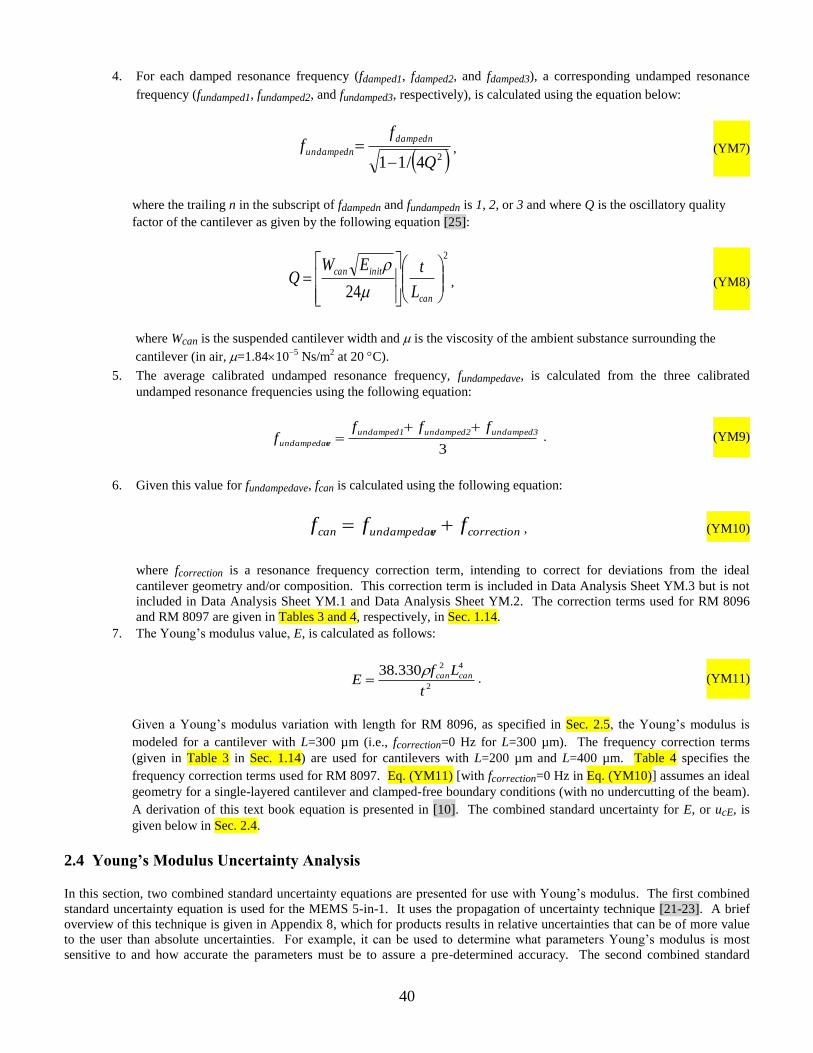
40

4. For each damped resonance frequency (fdamped1, fdamped2, and fdamped3), a corresponding undamped resonance

frequency (fundamped1, fundamped2, and fundamped3, respectively), is calculated using the equation below:

24/11 Q

ff

dampedn

undampedn

, (YM7)

where the trailing n in the subscript of fdampedn and fundampedn is 1, 2, or 3 and where Q is the oscillatory quality

factor of the cantilever as given by the following equation [25]:

2

24

can

initcan

L

tEWQ

, (YM8)

where Wcan is the suspended cantilever width and is the viscosity of the ambient substance surrounding the

cantilever (in air, =1.84105

Ns/m2 at 20 C).

5. The average calibrated undamped resonance frequency, fundampedave, is calculated from the three calibrated

undamped resonance frequencies using the following equation:

3

undamped3undamped2undamped1

eundampedav

ffff

. (YM9)

6. Given this value for fundampedave, fcan is calculated using the following equation:

correctioneundampedavcan fff , (YM10)

where fcorrection is a resonance frequency correction term, intending to correct for deviations from the ideal

cantilever geometry and/or composition. This correction term is included in Data Analysis Sheet YM.3 but is not

included in Data Analysis Sheet YM.1 and Data Analysis Sheet YM.2. The correction terms used for RM 8096

and RM 8097 are given in Tables 3 and 4, respectively, in Sec. 1.14.

7. The Young’s modulus value, E, is calculated as follows:

2

42330.38

t

LfE cancan . (YM11)

Given a Young’s modulus variation with length for RM 8096, as specified in Sec. 2.5, the Young’s modulus is

modeled for a cantilever with L=300 µm (i.e., fcorrection=0 Hz for L=300 µm). The frequency correction terms

(given in Table 3 in Sec. 1.14) are used for cantilevers with L=200 µm and L=400 µm. Table 4 specifies the

frequency correction terms used for RM 8097. Eq. (YM11) [with fcorrection=0 Hz in Eq. (YM10)] assumes an ideal

geometry for a single-layered cantilever and clamped-free boundary conditions (with no undercutting of the beam).

A derivation of this text book equation is presented in [10]. The combined standard uncertainty for E, or ucE, is

given below in Sec. 2.4.

2.4 Young’s Modulus Uncertainty Analysis

In this section, two combined standard uncertainty equations are presented for use with Young’s modulus. The first combined

standard uncertainty equation is used for the MEMS 5-in-1. It uses the propagation of uncertainty technique [21-23]. A brief

overview of this technique is given in Appendix 8, which for products results in relative uncertainties that can be of more value

to the user than absolute uncertainties. For example, it can be used to determine what parameters Young’s modulus is most

sensitive to and how accurate the parameters must be to assure a pre-determined accuracy. The second combined standard

41

uncertainty equation presented in this section is similar to that used in the MEMS Young’s modulus round robin. It adds

absolute uncertainties in quadrature.

2.4.1 Young’s Modulus Uncertainty Analysis for the MEMS 5-in-1

This section presents the combined standard uncertainty equation used with the MEMS 5-in-1. To obtain this equation, the

propagation of uncertainty technique [21-23] for parameters that multiply (see Appendix 8) is applied to Eq. (YM11). The

resulting one sigma uncertainty of the value of E, that is E, is given by:

2

2

2

2

22

2 242

can

fcan

can

LthickE

fLtE

, (YM12)

where thick is the one sigma uncertainty of the value of t, which is found using the electro-physical technique [6] for RM 8096

and found using the optomechanical technique [7] for RM 8097. The on-line version of Data Analysis Sheet T.1 [13], as

reproduced in Appendix 6, can be used to calculate t and thick for RM 8096. The on-line version of Data Analysis Sheet T.3.a

[13], as reproduced in Appendix 7, can be used to calculate t and thick for RM 8097. Also in the above equation, is the

estimated one sigma uncertainty of the value of , L is the estimated one sigma uncertainty of the value of Lcan, and fcan [as

obtained by applying the propagation of uncertainty technique [21-23] for parameters in an additive relationship (see Appendix

8) to Eq. (YM10)] is given by the following equation:

22

nfcorrectiovefundampedafcan , (YM13)

where

222

freqcalfresolfundampedvefundampeda , (YM14)

and

22

cantileverportsupnfcorrectio , (YM15)

where fundamped (the standard deviation of the calibrated undamped resonance frequency measurements) is given by the

following:

),,( 3undamped2undamped1undampedfundamped fffSTDEV , (YM16)

where fresol is calculated assuming a uniform distribution using the following equation:

32

fresol

fresol

calf , (YM17)

where fresol is the uncalibrated frequency resolution for the given set of measurement conditions. Also in Eq. (YM14), freqcal is

the one sigma uncertainty of the value of fundampedave due to the frequency calibration as given by the following equation:

meter

cmeter

eundampedavfreqcalf

uf , (YM18)

42

where fmeter is the average of the three measurements taken with the frequency meter in Sec. 2.2 and ucmeter is the uncertainty of

the three frequency measurements taken with the frequency meter for which the uncertainty is assumed to scale linearly.

In Eq. (YM15), support is the one sigma uncertainty in the resonance frequency due to a non-ideal support or attachment

conditions (such as any undercutting of the beam and remaining debris in the attachment corners of the cantilever to the beam

support as mentioned in Sec. 2.1 for RM 8096) and cantilever is the one sigma uncertainty in the resonance frequency due to

geometry or composition deviations from the ideal cantilever (such as the four oxide layers that comprise the cantilever

discussed in Sec. 2.1 for RM 8096 or the vertical transition discussed in Sec. 2.1 for RM 8097). Tables 3 and 4 in Sec. 1.14 give

the values of σsupport and σcantilever used for RM 8096 and RM 8097, respectively. Equation (YM15) assumes that σsupport and

cantilever are uncorrelated. If it is determined that they are correlated, set σsupport=0 Hz and include the uncertainty associated

with the support into cantilever.

Looking at Eq. (YM12), it is assumed that the one sigma uncertainty of the value of E, that is E, is equal to the combined

standard uncertainty, ucE. In this case,

E3cEu , (YM19)

where a number following the subscript “E” in “ucE” indicates the data analysis sheet that is used to obtain the combined

standard uncertainty value. Therefore, ucE3 implies that Data Analysis Sheet YM.3 is used. Combining Eq. (YM12), Eq.

(YM13), Eq. (YM14), Eq. (YM15), and Eq. (YM19) produces the following equation for the combined standard uncertainty:

2222

2222

4444

4164

can

cantilever

can

portsup

can

freqcal

can

fresol

can

fundamped

can

Lthick

3cE

ffff

fLtEu

, (YM20)

for use with the MEMS 5-in-1 where each component in Eq. (YM20) was obtained using a Type B analysis, except where

noted. The parameters specified in the denominators of the various ratios in Eq. (YM12) and Eq. (YM20) are the parameters in

the Young’s modulus equation given in Eq. (YM11). The parameters specified in the numerators are various standard

deviations of the parameter in the denominator, which makes each ratio a relative uncertainty. Table YM4 gives example values

for each of the uncertainty components as well as the combined standard uncertainty value, ucE3. Using the relative uncertainty

values, as given in Table YM4 for this approach, allows one to more easily determine the most influential parameters as well as

allowing one to determine how accurately the parameters must be determined to assure a pre-determined accuracy.

The expanded uncertainty for Young’s modulus, UE, is calculated using the following equation:

3cE3cEE ukuU 2 , (YM21)

where the k value of 2 gives an expanded uncertainty approximating a 95 % level of confidence.

Reporting results [21-23]: If it is assumed that the estimated values of the uncertainty components are approximately

Gaussianly distributed with approximate combined standard uncertainty ucE3, the Young’s modulus value is believed to lie in

the interval E ucE3 (expansion factor k=1) representing a level of confidence of approximately 68 %.

43

Table YM4. Example Young’s Modulus Uncertainty Values Using the MEMS 5-in-1 Approach as Given in Eq. (YM20)

uncertainty Type

A or B

uncertainty

values

1. t

thick

(using t=2.743 m and thick=0.058 m)

B

0.0211

2.

(using =2.2 g/cm3 and =0.05 g/cm

3)

B

0.023

3.

can

L

L

(using Lcan=300m and L=0.2 m)

B

0.00067

4.

22222

can

cantilever

can

portsup

can

freqcal

can

fresol

can

fundamped

can

fcan

ffffff

(using fmeas1 =26.82625 kHz,

fmeas2 =26.8351 kHz,


calf = 1, and Q= 65.8,

such that fundampedave= 26.8296 kHz

and using fcorrection= 0 kHz a

)

0.0002

4a.

can

fundamped

f

(using Wcan=28 m,

Einit=70 GPa,

and =1.8410

Ns/m2)

A

0.0002

4b.

can

fresol

f

(using fresol=1.25 Hz)

B

0.000013

4c.

can

freqcal

f

(using freqcal=0.0 Hz)a

B

0.0

4d.

can

portsup

f

(support and attachment assumed to be ideal, support=0 Hz) a

B 0.0

4e.

can

cantilever

f

(using cantilever=0 Hz) a

B 0.0

2222

4164

can

fcan

can

LthickE

fLtE

0.048

ucE3 = E

(using E = 65.35 GPa)

3.1 GPa

a This was assumed to be zero to more appropriately compare this data set with the Young’s modulus round robin data set in Table YM5.

44

2.4.2 Previous Young’s Modulus Uncertainty Analyses

For the second combined standard uncertainty equation (similar to that used in the MEMS Young’s modulus round robin

[10,34-35]), seven sources of uncertainty are identified with all other sources considered negligible. The seven sources of

uncertainty are the uncertainty of the thickness (uthick), the uncertainty of the density (u), the uncertainty of the cantilever

length (uL), the uncertainty of the average resonance frequency (ufreq), the uncertainty due to the frequency resolution (ufresol),

the uncertainty due to damping (udamp), and the uncertainty due to the frequency calibration (ufreqcal). As such, the combined

standard uncertainty equation for ucE with seven sources of uncertainty is as follows:

2222222

freqcaldampfresolfreqLthick2Ec uuuuuuuu , (YM22)

where a number following the subscript “E” in “ucE” indicates the data analysis sheet that is used to obtain the combined

standard uncertainty value. Therefore, ucE2 implies that Data Analysis Sheet YM.2 [13] is used. [The equation for ucE1, which

uses Data Analysis Sheet YM.1, does not include the last uncertainty component, ufreqcal, in Eq. (YM22) and is the actual

combined standard uncertainty equation used in the MEMS Young’s modulus round robin.] In determining the combined

standard uncertainty, a statistical Type A evaluation is used for ufreq. The other sources of uncertainty are obtained using a Type

B evaluation [21-23]. Table YM5 gives sample values for each of the uncertainty components in Eq. (YM22) assuming that

ufreqcal=0 GPa such that the combined standard uncertainty value ucE1 is also given in Table YM5. Note that the resulting

values for ucE3 (3.1 GPa in Table YM4) and ucE1 (3.2 GPa in Table YM5) are comparable.

Table YM5. Example Young’s Modulus Uncertainty Values, From a Round Robin Bulk-Micromachined

CMOS Chip (Assuming Einit=70 GPa), Comparable to Those Obtained in Table YM4

source of uncertainty or descriptor uncertainty values

1. uthick

thickness 2.8 GPa

(using t=2.743 m and thick=0.058 m)

2. u

density 1.5 GPa

(using =2.2 g/cm3 and =0.05 g/cm

3)

3. uL

cantilever length 0.17 GPa

(using Lcan=300m and L=0.2 m)

4. ufreq

average resonance frequency 0.027 GPa

(using fmeas1 =26.82625 kHz,


and fmeas3 =26.8251 kHz)

5. ufresol

frequency resolution 0.0018 GPa

(using fresol=1.25 Hz)

6. udamp

damping 0.0004 GPa

(using Wcan=28 m and W=0.1 m and

using =1.8410

Ns/m2 and =0.0110

Ns/m

2)

ucE1a

combined standard uncertainty for Young’s modulus 3.2 GPa

= 222222

dampfresolfreqLthick uuuuuu

a This ucE1 uncertainty (times 3) is plotted in Fig. YM6 with the repeatability data point corresponding to the first cantilever with length of 300 m.

The first uncertainty component in Eq. (YM22) and listed in Table YM5 and Table YM6 is uthick. (Table YM6 provides the

equations for the uncertainty components.) The uncertainty for uthick is determined from the calculated minimum and maximum

Young’s modulus values (namely, Emin and Emax, respectively) as derived using the extremes of values expected for the

cantilever thickness. The values for Emin and Emax are given in the second and third columns, respectively, of Table YM6

where thick is the one sigma uncertainty of the value of t, as specified in Sec. 2.4.1. With 99.7 % nominal probability of

45

coverage, assuming a Gaussian distribution (and assuming u, uL, ufreq, ufresol, udamp, and ufreqcal equal zero), the value for E

lies between Emin and Emax. Therefore, uthick is calculated using the formula given in the fifth column of Table YM6.

Table YM6. Previous Young’s Modulus Uncertainty Equations [10,34-35]

Emin Emax G or Ua

/ A or Bb

equation

1. uthick

2

42

)3(

330.38

thick

cancan

t

Lf

2

42

)3(

330.38

thick

cancan

t

Lf

G / B

6

minmax EEuthick

2. u 2

423330.38

t

Lf cancan

2

423330.38

t

Lf cancan

G / B

6

minmax EEu

3. uL 2

42 3330.38

t

Lf Lcancan

2

42 3330.38

t

Lf Lcancan

G / B

6

minmax EEuL

4. ufreq 2

423330.38

t

Lf canfreqcan

2

423330.38

t

Lf canfreqcan

G / A

6

minmax EEu freq

5. ufresol

2

4

2

2330.38

t

Lcalf

f can

fresol

can

2

4

2

2330.38

t

Lcalf

f can

fresol

can

U / B 32

minmax EEu fresol

6. udamp 2

423330.38

t

Lf canfQcan

2

423330.38

t

Lf canfQcan

G / B

6

minmax EEudamp

7. ufreqcal 2

423330.38

t

Lf canfreqcalcan

2

423330.38

t

Lf canfreqcalcan

G / B

6

minmax EEu freqcal

a “G” indicates a Gaussian distribution and “U” indicates a uniform distribution

b Type A or Type B analysis

In the same way, using the formulas in Table YM6, the remaining uncertainty components in Eq. (YM22) are calculated, where

and L are given in Sec. 2.4.1, where freq is the standard deviation of fundamped1, fundamped2, and fundamped3 [also called

σfundamped in Eq. (YM16) in Sec. 2.4.1], and where fQ is the one sigma uncertainty of the value of fcan due to damping as

mostly detailed in [10,34-35].20

[If undamped resonance frequencies (e.g., if the measurements were performed in a vacuum)

were obtained and recorded as fmeas1, fmeas2, and fmeas3, then udamp is set equal to 0.0 Pa.]

2.5 Young’s Modulus Round Robin Results

The round robin repeatability and reproducibility results are given in this section for Young’s modulus measurements. The

repeatability measurements are performed using the same test method, in the same laboratory (NIST), by the same operator,

with the same equipment, in the shortest practical period of time (nominally, within a day). These measurements are done on

random test structures. For the reproducibility measurements, at least six independent data sets (each using a different piece of

equipment or equipment setup) must be obtained following the same test method before the results can be recorded in the

precision and bias statement of a SEMI standard test method. These measurements are also done on random test structures.

The repeatability data were taken in one laboratory using a dual beam vibrometer (see Sec. 1.1.1 for specifications of the

vibrometer used in this procedure). The round robin test chips were processed using a bulk-micromachined CMOS process,

20

For Data Sheet YM.2 [13], the approach in [10] is slightly modified to include the uncertainty due to the frequency calibration.

46

similar to that used for RM 8096 depicted in Fig. 1. A total of 48 Young’s modulus values were obtained from twelve different

cantilevers four times, with each Young’s modulus value determined from the average of three resonance frequency

measurements. Of these values, 16 were from four different cantilevers with L=200 m, 16 from four different cantilevers with

L=300 m, and 16 from four different cantilevers with L=400 m.

For the reproducibility data, eight participants were identified.21

Each participant was supplied with a round robin test chip and

asked to obtain three Young’s modulus values; one from an oxide cantilever with a design length of 200 m, one from an oxide

cantilever with a design length of 300 m, and one from an oxide cantilever with a design length of 400 m. (The participant

could choose to measure any one of five cantilevers of the given length as long as it passed a visual inspection.) Each Young’s

modulus value was determined from the average of three resonance frequency measurements from the cantilever as specified in

Sec. 2.3, using an instrument that meets the manufacturer’s alignment and calibration criteria. Following SEMI standard test

method MS4 for Young’s modulus measurements [35], the measurements were taken then recorded on Data Analysis Sheet

YM.1 [13].

The eight participants used a variety of instruments to obtain Young’s modulus. These included a single beam vibrometer, a

dual beam vibrometer, and a stroboscopic interferometer (consult Sec. 1.1.1 for details associated with these instruments). In

addition, thermal excitation measurements [36-38] were obtained on the same chip as PZT excitation measurements and the

results are included for comparison purposes.

Tables YM7 and YM8 present the Young’s modulus repeatability and reproducibility results, respectively. In these tables, n

indicates the number of calculated Young’s modulus values. The average (namely Eave) of the repeatability or reproducibility

measurement results is listed next, followed by the standard deviation (σE) of these measurements. Then, the ±2σE limits are

given followed by the average of the repeatability or reproducibility combined standard uncertainty values (ucE1ave).

The Young’s modulus repeatability and reproducibility results are plotted in Fig. YM6. At the top of this figure, Eave and

3ucE1ave are specified for the repeatability data. The values for Eave ± 3ucE1ave are also plotted in this figure with both the

repeatability22

and reproducibility data. As an observation, all of the reproducibility results fall comfortably between the

repeatability bounds of Eave ± 3ucE1ave.

Table YM7. Young’s Modulus Repeatability Data

(One Participant, One Laboratory, One Instrument, One Chip, Twelve Different Cantilevers)

Lcan=200 m

Lcan=300 m

Lcan=400 m

Lcan=200 m

to

Lcan=400 m

n 16 16 16 48

Eave 59.8 GPa 65.4 GPa 67.5 GPa 64.2 GPa

σE 0.40 GPa 0.17 GPa 0.38 GPa 3.3 GPa

±2σE limits ±0.81 GPa

(±1.4 %)

±0.33 GPa

(±0.51 %)

±0.76 GPa

(±1.1 %)

±6.6 GPa

(±10 %)

ucE1ave 2.9 GPa

(4.9 %)

3.2 GPa

(4.8 %)

3.3 GPa

(4.8 %)

3.1 GPa

(4.8 %)

21

The term participant refers to a single data set from a unique combination of measurement setup and researcher. In other words, a single researcher with

multiple, unique instruments (e.g., a dual beam vibrometer and a single beam vibrometer) or different forms of excitation (e.g., PZT and thermal excitation)

could serve as multiple “participants.” 22

Table YM5 specifies the value of each of the uncertainty components comprising ucE1 for a Young’s modulus measurement where the 3ucE1 uncertainty bars

for this measurement are associated with the repeatability data point for the first cantilever in Fig. YM6 with a length of 300 m.

47

Table YM8. Young’s Modulus Reproducibility Data

(Eight Participants, Five Laboratories, Seven Instruments, Four Chips)

Lcan=200 m

Lcan=300 m

Lcan=400 m

Lcan=200 m

to

Lcan=400 m

n 8 8 8 24

Eave 58.7 GPa 63.7 GPa 66.0 GPa 62.8 GPa

σE 1.3 GPa 1.8 GPa 1.4 GPa 3.4 GPa

±2σE limits ±2.6 GPa

(±4.4 %)

±3.5 GPa

(±5.5 %)

±2.9 GPa

(±4.4 %)

±6.9 GPa

(±11 %)

ucE1ave 2.8 GPa

(4.9 %)

3.1 GPa

(4.8 %)

3.2 GPa

(4.9 %)

3.0 GPa

(4.9 %)

In Fig. YM6, the repeatability data are grouped according to the cantilever length with the L=200 m data plotted first, followed

by the L=300 m data, then the L=400 m data. The same is done with the reproducibility data where for each participant, the

L=200 m data are plotted first, followed by the L=300 m data, then the L=400 m data. Both the repeatability data and the

reproducibility data indicate a length dependency. In Fig. YM6, the repeatability data show a clustering of the data at each

length. The absolute value of the ±2σE limits at each length (which are plotted in this figure along with Eave for each length) are

all less than 1.5 %, which is much less than the 10 % value (as given in Table YM7) when all the lengths are considered. This

suggests that when comparing Young’s modulus values extracted by different measurement instruments or excitation methods,

the cantilevers should have the same length. This length dependency can be due to a number of things including debris in the

attachment corners of the cantilevers to the beam support, which would cause larger errors for shorter length cantilevers. This

can be a topic for future investigation where a) the physical form and chemical composition of the cantilever is checked to see if

it matches the assumptions used in the calculations and b) finite element methods are used to determine if the length dependency

is due to the attachment conditions (including debris in the attachment corners of the cantilever and any undercutting of the

beam). Therefore, at this point, we can only state that, given the existing cantilevers, we can only report an “effective” value for

Young’s modulus.

As seen in Fig. YM6, round robin participant #1, participant #2, and participant #3 took measurements on the same chip (chip

#1) using a dual beam vibrometer, a single beam vibrometer, and a stroboscopic interferometer, respectively. The results

indicate that comparable results were obtained from these instruments.

Round robin participant #4, participant #5, and participant #6 took measurements on the same chip (chip #2) with participant #5

using thermal excitation to obtain the required data and participant #4 and participant #6 using PZT excitation. Fig. YM6 shows

no significant difference in the results.

Round robin participant #7 and participant #8 took data from chip #3 and chip #4, respectively.

No information can be presented on the bias of the procedure in the test method for measuring Young’s modulus because there

is not a certified MEMS material for this purpose. Many values for Young’s modulus for various materials have been published

with an attempt to consolidate this information in [33]. For a silicon dioxide film, the Young’s modulus values reported in [33]

range from 46 GPa to 92 GPa. The average repeatability value reported in Table YM7 of 64.2 GPa obtained from the oxide

cantilever that consists of field oxide, two depositied oxides and a glass layer falls comfortably within this range.

48

Figure YM6. Young’s modulus round robin results

23

2.6 Using the MEMS 5-in-1 to Verify Young’s Modulus Measurements

To compare your Young’s modulus measurements with NIST measurements, you will need to fill out Data Analysis Sheet

YM.3; this data analysis sheet is accessible via the URL specified in the reference [13], a reproduction of which is given in

Appendix 1. After obtaining an estimate for the resonance frequency, calibrating the instrument, locating the cantilever test

structure, taking the measurements, and performing the calculations, the data on the completed form can be compared with the

data on the RM Report of Investigation and the completed data analysis sheet supplied with the MEMS 5-in-1. Details of the

procedure are given below.

Obtain an estimate for the resonance frequency: To determine an estimate for the resonance frequency of the cantilever (that

may be a bit on the high side especially for shorter length cantilevers) do the following:

1. Access Data Analysis Sheet YM.3,

2. Supply inputs for:

a. (input #5),

b. t (input #9),

c. Einit (input #12), and

d. Lcan (input #19),

3. Press the “Calculate Estimates” button that appears before the Preliminary Estimates Table (Table 5) on the data

analysis sheet, and

4. The value for fcaninit (output #38) is the estimate for the resonance frequency.

Calibrate the instrument: Calibrate the time base of the instrument as given in Sec. 2.2. Obtain the inputs for Table 1 in Data

Analysis Sheet YM.3.

Locate the cantilever: In the first grouping of test structures on the MEMS 5-in-1 chips shown in Fig. 1 and Figs. 2(a and b) for

RM 8096 and RM 8097, respectively, Young’s modulus measurements are made. Cantilever and fixed-fixed beam test

structures are provided for this purpose; however, we will only be concerned with the cantilevers, such as shown in Fig. YM2

for RM 8096 and as shown in Figs. YM3 and YM4 for RM 8097. Specifications for the cantilevers in the Young’s modulus

grouping of test structures in Figs. YM1(a and b) for RM 8096 and RM 8097, respectively, are given in Table YM1.

23

Republished with permission from Semiconductor Equipment and Materials International, Inc. (SEMI) © 2011.

49

Data Analysis Sheet YM.3 requires measurements from one cantilever on the MEMS 5-in-1 chip. The specific cantilever to be

measured can be deduced from the data entered on the NIST-supplied Data Analysis Sheet YM.3 that accompanies the RM.

For the Young’s modulus grouping of test structures for RM 8096, as shown in Fig. YM1(a), the target test structure can be

found as follows:

1. The input Lcan (i.e., input #19 on Data Analysis Sheet YM.3) specifies the length of the cantilever. The length of

the cantilever (in micrometers) is given at the top of each column of cantilevers in Fig. YM1(a) following the

column number (i.e., 1 to 5), therefore Lcan can be used to locate the column in which the target cantilever resides.

2. The input whichcan (i.e., input #20) specifies which cantilever in the column to measure (i.e., the “first,” “second,”

“third,” etc.) regardless of the orientation.

3. The input orient (i.e., input #18) can be used as a form of verification. The cantilevers are designed at both a 0 and

a 180 orientation with the cantilevers having a 0 orientation being the first, second, and third cantilevers in each

column and the cantilevers with a 180 orientation being the fourth, fifth, and sixth cantilevers in each column.

Therefore, either 0 or 180 will be selected for orient.

For the Young’s modulus grouping of test structures for RM 8097, as shown in Fig. YM1(b), the target test structure can be

found as follows:

1. The input mat (i.e., input #4) specifies the composition of the cantilever, which should be either “poly1” or

“poly2” since there are two arrays of poly1 cantilevers and two arrays of poly2 cantilevers.

2. The input orient (i.e., input #18) can be used to locate the appropriate array since one of the two arrays of a given

composition has a 0 orientation and the other has a 90 orientation.

3. The input Lcan (i.e., input #19) can be used to locate the appropriate length cantilever within the array. Within

each array, the cantilevers are arranged by increasing length with the shortest cantilevers (Lcan=100 m) at the top

(or leftmost) part of the array and the longest cantilevers (Lcan=500 m) at the bottom (or rightmost) part of the

array.

4. The input whichcan (i.e., input #20) is used to identify which of the three identically designed cantilevers (the

“first,” “second,” or “third”) is the one to measure within the array. The length is specified to the left of or below

the anchor of the second of the three identical cantilevers.

Take the measurements: For Data Analysis Sheet YM.3, the uncalibrated frequency resolution (as specified by the software)

and three uncalibrated resonance frequency measurements are required for the cantilever. Obtain these measurements using the

highest magnification objective that is available and feasible (e.g., a 20 objective) following the steps in SEMI standard test

method MS4 [1] for measuring Young’s modulus.

Perform the calculations: Enter the data into Data Analysis Sheet YM.3 as follows:

1. Press one of the “Reset this form” buttons. (One of these buttons is located near the top of the data analysis sheet

and the other is located near the middle of the data analysis sheet.)

2. Fill out Table 1 and Table 2. (Table 4 is needed for residual stress and stress gradient calculations, as indicated in

Sec. 7.3.)

3. Press one of the “Calculate and Verify” buttons to obtain the results for the cantilever. (One of these buttons is

located near the top of the data analysis sheet and the other is located near the middle of the data analysis sheet.)

4. Verify the data by checking to see that all the pertinent boxes in the verification section at the bottom of the data

analysis sheet say “ok”. If one or more of the boxes say “wait,” address the issue, if necessary, by modifying the

inputs and recalculating.

5. Print out the completed data analysis sheet to compare both the inputs and outputs with those on the NIST-supplied

data analysis sheet.

Compare the measurements: The MEMS 5-in-1 is accompanied by a Report of Investigation. This Report of Investigation

specifies an effective Young’s modulus value, E, and the expanded uncertainty, UE, (with k=2) intending to approximate a 95 %

level of confidence. It is your responsibility to determine an appropriate criterion for acceptance, such as given below:

22

)()( EcustomerEcustomerE UUEED , (YM23)

where DE is the absolute value of the difference between your Young’s modulus value, E(customer), and the Young’s modulus

value on the RM Report of Investigation, E, and where UE(customer) is your expanded uncertainty value and UE is the expanded

uncertainty on the RM Report of Investigation. If your measured value for Young’s modulus (as obtained in the newly filled out

50

Data Analysis Sheet YM.3) satisfies your criterion for acceptance and there are no pertinent “wait” statements at the bottom of

your Data Analysis Sheet YM.3, you can consider yourself to be appropriately measuring Young’s modulus according to the

SEMI MS4 Young’s modulus standard test method [1] according to your criterion for acceptance.

An effective Young’s modulus is reported for RM 8096, as shown in Fig. 1, and for RM 8097, as shown in Figs. 2(a and b), due

to deviations from the ideal geometry and/or composition of the cantilever and/or the beam support as specified in Sec. 2.1 and

Sec. 2.5. When you use SEMI standard test method MS4 with your own test structures, you must be cognizant of the geometry

and composition of your cantilever because this test method assumes an ideal geometry and composition, implying that you

would be obtaining an “effective” Young’s modulus value if the geometry and/or composition of your cantilever deviates from

the ideal.

Any questions concerning the measurements, analysis, or comparison can be directed to [email protected].


51

3 Grouping 2: Residual Strain

Residual strain is defined in a MEMS process as the amount of deformation (or displacement) per unit length constrained within

the structural layer of interest after fabrication yet before the constraint of the sacrificial layer (or substrate) is removed (in

whole or in part) [2]. It is a measurement of the strain the parts of a microsystem undergo before they relax after the removal of

the stiff oxides that surround them during manufacturing. ASTM standard test method E 2245 [2] on residual strain

measurements is an aid in the design and fabrication of MEMS devices [31-32].

This section on residual strain is not meant to replace but to supplement the ASTM standard test method E 2245 [2], which more

completely presents the scope, significance, terminology, apparatus, and test structure design as well as the calibration

procedure, measurement procedure, calculations, precision and bias data, etc. In this section, the NIST-developed residual strain

test structures on RM 8096 and RM 8097, as shown in Fig. 1 and Figs. 2(a and b) in the Introduction are presented in Sec. 3.1.

Sec. 3.2 discusses the calibration procedure for the residual strain measurements, and Sec. 3.3 discusses the residual strain

measurement procedure. Following this, the uncertainty analysis is presented in Sec. 3.4, the round robin results are presented

in Sec. 3.5, and Sec. 3.6 describes how to use the MEMS 5-in-1 to verify residual strain measurements.

3.1 Residual Strain Test Structures

Residual strain measurements are taken in the second grouping of test structures, as shown in Fig. RS1(a) for RM 8096 depicted

in Fig. 1, as shown in Fig. RS1(b) for RM 8097 (fabricated on MUMPs98) depicted in Fig. 2(a), and as shown in Fig. RS1(c) for

RM 8097 (fabricated on MUMPs95) depicted in Fig. 2(b).

(a) (b) (c)

Figure RS1. The residual strain grouping of test structures on (a) RM 8096, fabricated on a multi-user 1.5 m CMOS process

[8] followed by a bulk-micromachining etch, as depicted in Fig. 1, (b) RM 8097 (fabricated on MUMPs98), as depicted in Fig.

2(a), and (c) RM 8097 (fabricated on MUMPs95), as depicted in Fig. 2(b), where (b) and (c) were processed using a polysilicon

multi-user surface-micromachining MEMS process [9] with a backside etch.

Residual strain measurements are obtained from fixed-fixed beam test structures. A fixed-fixed beam test structure in the

residual strain grouping of test structures, as shown in Figs. RS1(a and c), can be seen in Fig. RS2(a) and Fig. RS3(a),

respectively, for the bulk-micromachined chip (RM 8096) and the surface-micromachined chip (RM 8097 fabricated on

MUMPs95) with a backside etch. Applicable data traces taken from these test structures are given in Figs. RS2(b and c) and

Figs. RS3(b and c), respectively.

y

x

52

(a)

(b)

(c)

Figure RS2. For a fixed-fixed beam test structure on RM 8096, (a) a design rendition,

(b) an example of a 2D data trace used to determine L in (a),24

and (c) an example of a 2D data trace taken along the length of the fixed-fixed beam in (a).25

24

Copyright, ASTM International, 100 Barr Harbor Drive, West Conshohocken, PA 19428, USA. Reproduced via permissions

with ASTM International. 25

Ibid.

-25

-20

-15

-10

-5

0

5

10

0 0.2 0.4 0.6 0.8 1 1.2

z(µ

m)

x (mm)

Data along Trace a΄, a, e or e΄

Edge 1 Edge 2

4

6

8

10

12

14

16

0 0.2 0.4 0.6 0.8 1 1.2

z(µ

m)

x (mm)

Data along Trace b, c, or d

L Edge 1 Edge 2

y

x

a

b c

d

e

exposed silicon

to be etched

(design layers

include active

area, contact,

via, and glass)

metal2 (m2)

dimensional

marker

etch stop

(n-implant

encompassing

active area) 16 m 16 m

e΄

a΄

53

a)

(b)

(c)

Figure RS3. For a p2 fixed-fixed beam test structure, (a) a design rendition on RM 8097 (fabricated on MUMPs95)

depicted in Fig. RS1(c), (b) an example of a 2D data trace used to determine L, and

(c) an example of a 2D data trace taken along the length of a fixed-fixed beam.

54

The specifications for the fixed-fixed beams shown in Figs. RS1(a, b, and c) for RM 8096 and RM 8097 are given in Table RS1.

Table RS1. Fixed-Fixed Beam Configurations for Residual Strain Measurements

RM Width

(m)

Length

(m)

Structural

Layer

Orientation Quantity of Beams

RM 8096 40 200, 248,

300, 348,

400

oxide 0 three of each length

(or 15 beams)

RM 8097 16 400, 450,

500, 550,

600, 650,

700, 750,

800

poly1 0 three of each length

(or 27 beams)

90 three of each length

(or 27 beams)


(or 27 beams)

For RM 8096: On RM 8096, all oxide fixed-fixed beams shown in Fig. RS1(a) are designed with a 0 orientation. As seen in

this figure, the length of a fixed-fixed beam (in micrometers) is given at the top of each column of fixed-fixed beams following

the column number (i.e., 1 to 5) and the letters “FF” to indicate a fixed-fixed beam. These design lengths (and the design width)

are specified in Table RS1. There are three fixed-fixed beams designed at each length. Therefore, there are 15 oxide fixed-

fixed beams with a 0 orientation.

As specified in Sec. 1.4.1, the exposed silicon, as shown in Fig. RS2(a), is isotropically etched in XeF2 to release the fixed-fixed

beam by removing the silicon around and beneath the beam. The dimensional markers are instrumental in firming up the

support region. They also can be used to measure the small amount of SiO2 that has also been etched in XeF2,26

which would

have the effect of modifying the in-plane length of the fixed-fixed beam. The etch stop, also shown in this figure, helps to

inhibit the etch away from the test structure to shield neighboring structures from the etch. It consists of an n-implant designed

to surround active area. Figs. YM2(a, b, and c) show a cantilever test structure on RM 8096. As can be seen in Fig. YM2(c),

there is undercutting of the cantilever. This is the case for fixed-fixed beams as well.

An oxide fixed-fixed beam consists of four SiO2 layers. The thickness of these beams is calculated using Data Analysis Sheet

T.1. See Sec. 8 for specifics. Even though the beam is made up of four layers of SiO2, the layers may not have the same

properties. Also there may be remaining debris in the attachment corners of the fixed-fixed beam to the beam support. Due to

these deviations from the ideal geometry and composition of the fixed-fixed beam and/or beam support [and including the

undercutting of the beam shown in Fig. YM2(c)] an effective residual strain is reported on the RM Report of Investigation,

presented in Sec. 3.6.

For RM 8097: On RM 8097, there are three arrays of fixed-fixed beams for residual strain measurements, as shown in Figs.

RS1(b and c). Two of these arrays consist of poly1 fixed-fixed beams (as indicated by a “P1” symbol) and one array consists of

poly2 fixed-fixed beams (as indicated by a “P2” symbol). The fixed-fixed beams within the top poly1 array have a 90

orientation, and the remaining poly1 array along with the poly2 array have fixed-fixed beams with a 0 orientation. The design

dimensions of the fixed-fixed beams are given in Table RS1.

Fig. RS3(a) shows one of the poly2 fixed-fixed beams in the residual strain grouping of test structures shown in Fig. RS1(c) for

RM 8097 (fabricated on MUMPs95). The poly2 fixed-fixed beam pad designs shown in Fig. RS3(a) are similar to the pad

design shown for the cantilever given in Fig. YM4(a). [For the chips fabricated on MUMPs98, in the residual strain grouping of

test structures, the poly2 anchor lip in each pad is extended an additional 2 µm (on the same side as the beam only) to make the

poly2 layer in the pad 76 µm × 78 µm. This provides more interferometric data points on the poly2 layer before any additional

topographic changes are noticeable by the interferometric microscope.]27

The pad includes both poly1 and poly2. By including

poly1 in the anchor design, the poly1 and poly2 fuse during the fabrication process to make a more rigid and reliable attachment

point.

26

The design dimension from the dimensional marker to the exposed silicon is 16 m, as shown in Fig. RS2(a). 27

In like manner, the poly1 fixed-fixed beam pad designs on RM 8097 (fabricated on MUMPs95) are similar to the pad design shown for the cantilever given in

Fig. YM3(a). For the chips fabricated on MUMPs98, in the residual strain grouping of test structures, the protruding poly1 anchor lip in each pad is extended an

additional 2 µm (on the same side as the beam only) to make the poly1 layer in the pad 76 µm × 78 µm, which provides more interferometric data points on the exposed poly1.

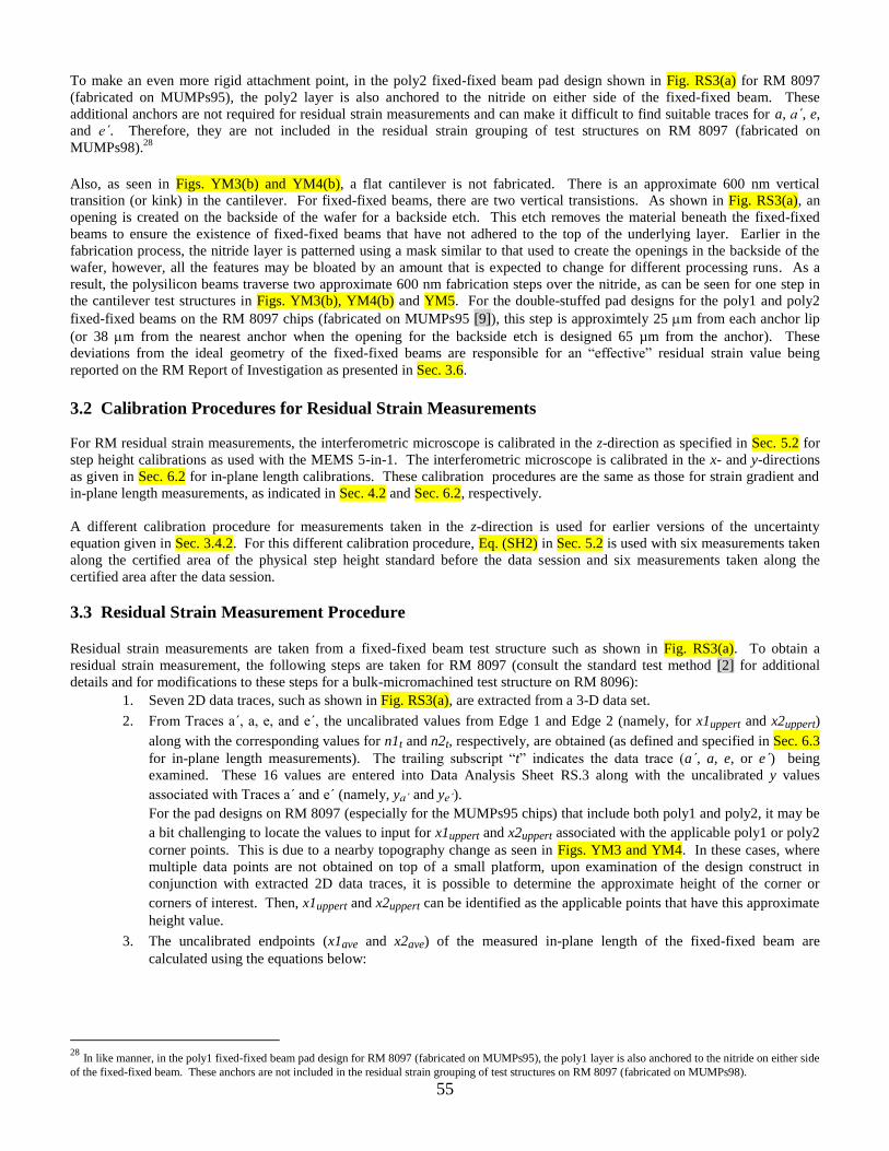
55

To make an even more rigid attachment point, in the poly2 fixed-fixed beam pad design shown in Fig. RS3(a) for RM 8097

(fabricated on MUMPs95), the poly2 layer is also anchored to the nitride on either side of the fixed-fixed beam. These

additional anchors are not required for residual strain measurements and can make it difficult to find suitable traces for a, a΄, e,

and e΄. Therefore, they are not included in the residual strain grouping of test structures on RM 8097 (fabricated on

MUMPs98).28

Also, as seen in Figs. YM3(b) and YM4(b), a flat cantilever is not fabricated. There is an approximate 600 nm vertical

transition (or kink) in the cantilever. For fixed-fixed beams, there are two vertical transistions. As shown in Fig. RS3(a), an

opening is created on the backside of the wafer for a backside etch. This etch removes the material beneath the fixed-fixed

beams to ensure the existence of fixed-fixed beams that have not adhered to the top of the underlying layer. Earlier in the

fabrication process, the nitride layer is patterned using a mask similar to that used to create the openings in the backside of the

wafer, however, all the features may be bloated by an amount that is expected to change for different processing runs. As a

result, the polysilicon beams traverse two approximate 600 nm fabrication steps over the nitride, as can be seen for one step in

the cantilever test structures in Figs. YM3(b), YM4(b) and YM5. For the double-stuffed pad designs for the poly1 and poly2

fixed-fixed beams on the RM 8097 chips (fabricated on MUMPs95 [9]), this step is approximtely 25 m from each anchor lip

(or 38 m from the nearest anchor when the opening for the backside etch is designed 65 µm from the anchor). These

deviations from the ideal geometry of the fixed-fixed beams are responsible for an “effective” residual strain value being

reported on the RM Report of Investigation as presented in Sec. 3.6.

3.2 Calibration Procedures for Residual Strain Measurements

For RM residual strain measurements, the interferometric microscope is calibrated in the z-direction as specified in Sec. 5.2 for

step height calibrations as used with the MEMS 5-in-1. The interferometric microscope is calibrated in the x- and y-directions

as given in Sec. 6.2 for in-plane length calibrations. These calibration procedures are the same as those for strain gradient and

in-plane length measurements, as indicated in Sec. 4.2 and Sec. 6.2, respectively.

A different calibration procedure for measurements taken in the z-direction is used for earlier versions of the uncertainty

equation given in Sec. 3.4.2. For this different calibration procedure, Eq. (SH2) in Sec. 5.2 is used with six measurements taken

along the certified area of the physical step height standard before the data session and six measurements taken along the

certified area after the data session.

3.3 Residual Strain Measurement Procedure

Residual strain measurements are taken from a fixed-fixed beam test structure such as shown in Fig. RS3(a). To obtain a

residual strain measurement, the following steps are taken for RM 8097 (consult the standard test method [2] for additional

details and for modifications to these steps for a bulk-micromachined test structure on RM 8096):

1. Seven 2D data traces, such as shown in Fig. RS3(a), are extracted from a 3-D data set.

2. From Traces a΄, a, e, and e΄, the uncalibrated values from Edge 1 and Edge 2 (namely, for x1uppert and x2uppert)

along with the corresponding values for n1t and n2t, respectively, are obtained (as defined and specified in Sec. 6.3

for in-plane length measurements). The trailing subscript “t” indicates the data trace (a΄, a, e, or e΄) being

examined. These 16 values are entered into Data Analysis Sheet RS.3 along with the uncalibrated y values

associated with Traces a΄ and e΄ (namely, ya΄ and ye΄).

For the pad designs on RM 8097 (especially for the MUMPs95 chips) that include both poly1 and poly2, it may be

a bit challenging to locate the values to input for x1uppert and x2uppert associated with the applicable poly1 or poly2

corner points. This is due to a nearby topography change as seen in Figs. YM3 and YM4. In these cases, where

multiple data points are not obtained on top of a small platform, upon examination of the design construct in

conjunction with extracted 2D data traces, it is possible to determine the approximate height of the corner or

corners of interest. Then, x1uppert and x2uppert can be identified as the applicable points that have this approximate

height value.

3. The uncalibrated endpoints (x1ave and x2ave) of the measured in-plane length of the fixed-fixed beam are

calculated using the equations below:

28

In like manner, in the poly1 fixed-fixed beam pad design for RM 8097 (fabricated on MUMPs95), the poly1 layer is also anchored to the nitride on either side

of the fixed-fixed beam. These anchors are not included in the residual strain grouping of test structures on RM 8097 (fabricated on MUMPs98).

56

4

eupperuppereupperaaupper

ave

1x1x1x1x1x

, and (RS1)

4

eupperuppereupperaaupper

ave

2x2x2x2x2x

. (RS2)

4. As specified in Sec. 6.3, the misalignment angle, α, is shown in Fig. L5(a), where Lmeas and Lalign in this figure are

calculated using Eqs. (L2) through (L4). The misalignment angle is typically determined using the two outermost

data traces [a΄ and e΄ in this case, as seen in Figs. RS3(a) and L5(b)] and is calculated to be either α1 or α2 using

either Δx1 or Δx2, respectively [as seen in Fig. L5(b)]. The equations for Δx1 and Δx2 are:

eupperaupper 1x1x1x , and (RS3)

eupperaupper 2x2x2x . (RS4)

The equation for α is as follows:

y

x

cal

cal

y

x1tan , where (RS5)

ea yyy . (RS6)

In addition,

if

,eaea 2n2n1n1n then1 and ,1xx (RS7)

if

,eaea 2n2n1n1n then2 and 2.xx (RS8)

5. The 2D data along the fixed-fixed beam from Traces b, c, and d, as shown in Fig. RS3(c) for one data trace, are

used to obtain three independent measurements of the curved length of the fixed-fixed beam. This is done for one

data trace as follows:

a. Eliminate the data values at both ends of the trace that will not be included in the modeling. This would

include all data values outside and including Edges 1 and 2 in Figs. RS3(a and b). If not already

eliminated, the data values less then x1ave and the data values greater than x2ave should also be

eliminated. In addition, for the 2D data trace given in Fig. RS3(c), the data values outside and including

Edges 7 and 8, if present, should be eliminated. [For the test structure shown in Fig. RS3(a), a backside

etch is used. As a result, for the process used, the beam traverses two approximate 600 nm fabrication

steps over the nitride used in conjunction with the backside etch (as specified in Sec. 3.1). One of these

steps can be seen in the cantilever test structures in Fig. YM4(b) and Fig. YM5. Due to these fabrication

steps, the data values outside and including Edges 7 and 8 are eliminated.]

b. Divide the remaining data into two data sets (as shown in Fig. RS4) if there is a peak (or valley) within

the length of the curved structure. [The division should occur at the x value corresponding to the

maximum (or minimum) z value. This data point should be included in both data sets.]

c. Choose three representative data points (sufficiently separated) within each data set. The three

uncalibrated points within the first data set are called (x1F, z1F), (x2F, z2F), and (x3F, z3F). And, the three

uncalibrated points within the second data set are called (x1S, z1S), (x2S, z2S), and (x3S, z3S), with x3F = x1S

and z3F = z1S as specified above, so that only five points are obtained from the data trace. In choosing

these points x3F is typically the x value corresponding to the maximum (or minimum) z value, (x2F, z2F)

and (x2S, z2S) are located near the inflection points, and x1F is slightly larger than x1ave (or an estimate of

57

x7ave if Edge 7 is present) and x3S is slightly smaller than x2ave (or an estimate of x8ave if Edge 8 is

present). The five uncalibrated data points are entered into Data Analysis Sheet RS.3.

d. To account for the misalignment angle, α, as shown in Fig. RS5, and the x-calibration factor, calx, the

values obtained above for x1ave, x1F, x2F, x3F = x1S, x2S, x3S, and x2ave become f, g, h, i, j, k, and l,

respectively, along the v-axis (the axis used to measure the length of the fixed-fixed beam) as also shown

in Fig. RS5. The uncalibrated z-values of the data points along the beam remain the same, which assumes

there is no curvature of the fixed-fixed beam across the width of the fixed-fixed beam. Therefore, the

calibrated data points along the beam become (g, z1F calz), (h, z2F calz), (i, z3F calz) or (i, z1S calz), (j, z2S

calz), and (k, z3S calz). The equations for f, g, h, i, j, k, and l are given below:

xavecal1xf , (RS9)

ffcalxg x1F cos , (RS10)

ffcalxh x2F cos , (RS11)

ffcalxffcalxi x1Sx3F coscos , (RS12)

ffcalxj x2S cos , (RS13)

ffcalxk x3S cos , and (RS14)

ffcal2xl xave cos . (RS15)

e. The in-plane length of the fixed-fixed beam, L, as shown in Fig. RS5, is calculated using the following

equation:

offsetalign LLL (RS16)

offsetLfl

,cos offsetxavexave Lcal1xcal2x

where Loffset is entered into Data Analysis Sheet RS.3 as the in-plane length correction term for the given

type of in-plane length measurement on similar structures when using similar calculations and for the

given magnification of the given interferometric microscope. See Sec. 6.3 for additional details. One

endpoint, v1end, of the in-plane length, L, is given below:

offsetxaveoffsetend Lcal1xLf1v2

1

2

1 , (RS17)

and the other endpoint, v2end, of L is as follows:

offsetxaveoffsetend Lffcal2xLl2v2

1cos

2

1 (RS18)

.2

1cos offsetxavexavexave Lcal1xcal1xcal2x

58

These endpoints are used next in the determination of the curved length of the fixed-fixed beam.

f. Using g, h, i, j, and k, as shown in Fig. RS5, two cosine functions (as seen in Fig. RS6) are used to model

the out-of-plane shape of the fixed-fixed beam and obtain the curved length, Lc, of the beam [with the v-

values of the endpoints given in Eqs. (RS17) and (RS18)].

6. The curved length of the fixed-fixed beam, Lc, for the given data trace, is compared with the in-plane length for a

calculation of residual strain, rt, using the following equation [14]:

nrcorrectiort LLL 1/ 00 , (RS19)

where L0 = [12 Lc (Lc Le / L)2] / [12(Lc Le / L)

2 2

t2] , so that (RS20)

rt={{L[12Lc(LcLe/L)2]/[12(LcLe/L)

22

t2]}/{[12Lc(LcLe/L)

2]/[12(LcLe/L)

22

t2]}}(1+δεrcorrection) , (RS21)

where L0 is the length with zero force applied, Le is the effective length of the fixed-fixed beam when the forces

Pc and P+ are applied, t is the thickness of the beam as obtained using Data Analysis Sheet T.1 for RM 8096 and

Data Analysis Sheet T.3.a for RM 8097, and where δεrcorrection is a relative residual strain correction term intended

to correct for deviations from the ideal fixed-fixed beam geometry and/or composition as discussed in more detail

in the next step. For a more complete description of these lengths, the forces mentioned, and the derivation of

these equations (without the correction term), consult reference [14]. The subscript “t” in rt refers to the data

trace used to obtain this residual strain value.

7. The relative residual strain correction term, δεrcorrection, is intended to correct for deviations from the ideal fixed-

fixed beam geometry and/or composition. This includes deviations from the ideal in both the beam support and

the beam itself (such as vertical transitions along the beam as discussed in Sec. 3.1 for RM 8097). For RM 8096

and 8097, it is currently assumed that δεrcorrection=0 and an effective value for residual strain is entered on the RM

Report of Investigation.

8. The resulting residual strain value, r, is the average of the residual strain values obtained from Traces b, c, and d,

as given below:

.3

rdrcrb

r

(RS22)

59

Figure RS4. Two data sets derived from an abbreviated data trace along a fixed-fixed beam.

The data in the figure above have been exaggerated.

Figure RS5. Sketch used to derive the appropriate v-values (f, g, h, i, j, k, and l) along the length of the beam

z

x

x1F x3F= x1S x3S

x2F x2S

x1ave x2ave

Data Derived from Trace b, c, or d

(x1F, z1F)

(x2F, z2F)

(x3F, z3F) = (x1S, z1S)

(x2S, z2S)

(x3S, z3S)

Trace a΄

Trace e΄

Edge 2 Edge 1

g h

i

j

k l

Loffset/2

Loffset/2

x3F calx = x1S calx x2S calx

x3S calx

x2F calx

x1F calx x2ave calx

α

L

Lalign

f=x1ave calx

v

60

Figure RS6. A comparison plot of the model with the derived data for an upward bending fixed-fixed beam.

The endpoints are not included in this plot.

3.4 Residual Strain Uncertainty Analysis

In this section, uncertainty equations are presented for use with residual strain. The first uncertainty equation (presented in Sec.

3.4.1) is used for the MEMS 5-in-1. The equations used in the round robin experiment and other previous work are presented in

Sec. 3.4.2.

3.4.1 Residual Strain Uncertainty Analysis for the MEMS 5-in-1

For the MEMS 5-in-1, the combined standard uncertainty, ucr3, for residual strain measurements with 13 uncertainty

components is given by the following equation:

2

)(

2222

)(

22222222

samprepeatcorrectionlineardriftshsrepeat

certnoiseRavexresxcalzresLW

3rcuuuuu

uuuuuuuuu

, (RS23)

with additional sources of uncertainty considered negliglible. A number following the subscript “r” in “ucr” indicates the data

analysis sheet that is used to obtain the combined standard uncertainty value. Therefore, ucr3 implies that Data Analysis Sheet

RS.3 [2,13] is used.

In Eq. (RS23), uW is the uncertainty due to variations across the width of the beam, uL is due to the measurement uncertainty of

L (without including the calibration uncertainty), uzres is the uncertainty due to the resolution of the interferometer in the z-

direction, uxcal is the uncertainty due to the calibration in the x-direction, and uxres is the uncertainty due to the resolution of the

interferometric microscope in the x-direction. Next, uRave is the uncertainty due to the sample’s surface roughness, unoise is the

uncertainty due to interferometric noise, ucert is due to the uncertainty of the value of the physical step height standard,

urepeat(shs) is the uncertainty due to the repeatability of a measurement taken on the physical step height standard, udrift is the

uncertainty due to the amount of drift during the data session, and ulinear is the uncertainty due to the deviation from linearity of

the data scan. Then, in Eq. (RS23), ucorrection is the uncertainty in the residual strain correction term due to non-ideal support

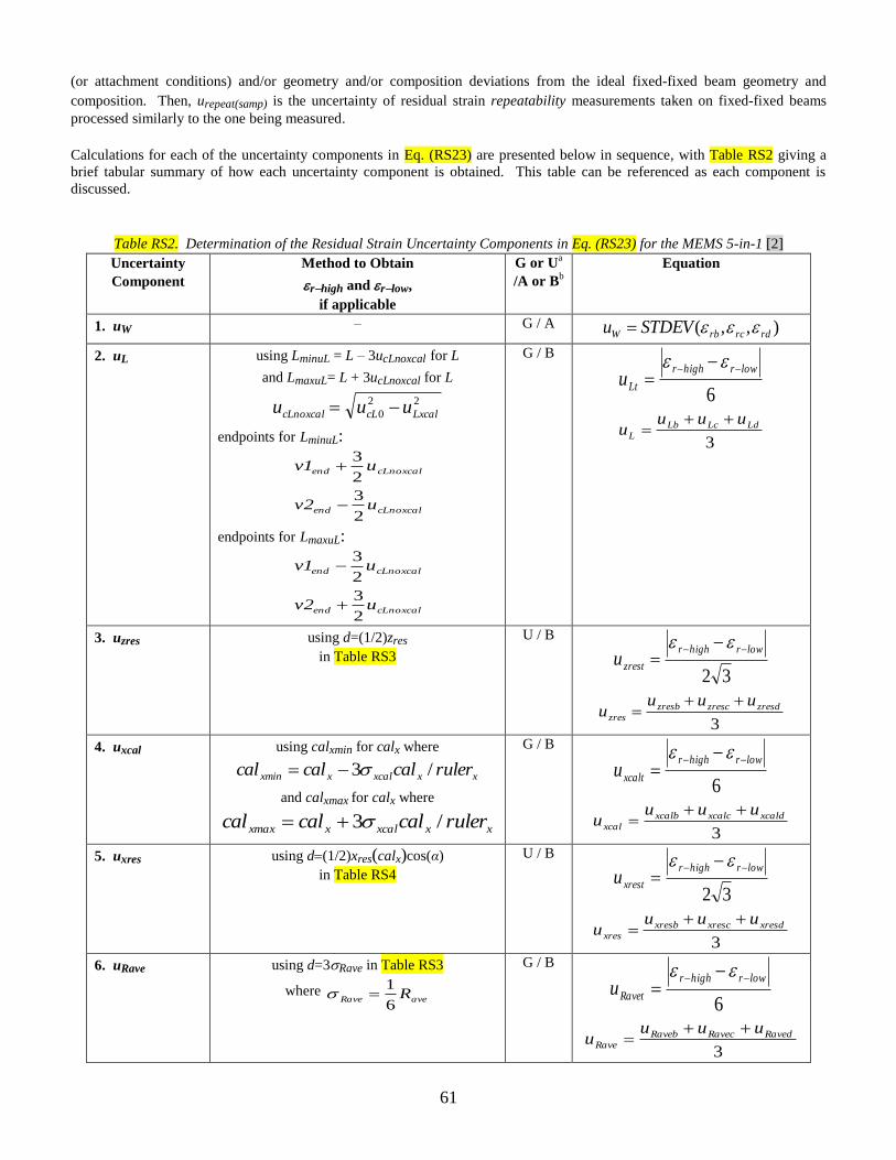
61

(or attachment conditions) and/or geometry and/or composition deviations from the ideal fixed-fixed beam geometry and

composition. Then, urepeat(samp) is the uncertainty of residual strain repeatability measurements taken on fixed-fixed beams

processed similarly to the one being measured.

Calculations for each of the uncertainty components in Eq. (RS23) are presented below in sequence, with Table RS2 giving a

brief tabular summary of how each uncertainty component is obtained. This table can be referenced as each component is

discussed.

Table RS2. Determination of the Residual Strain Uncertainty Components in Eq. (RS23) for the MEMS 5-in-1 [2]

Uncertainty

Component

Method to Obtain

rhigh and rlow,

if applicable

G or Ua

/A or Bb

Equation

1. uW – G / A ),,( rdrcrbW STDEVu

2. uL using LminuL = L – 3ucLnoxcal for L

and LmaxuL= L + 3ucLnoxcal for L

22

0 LxcalcLcLnoxcal uuu

endpoints for LminuL:

cLnoxcalend u1v2

3

cLnoxcalend u2v2

3

endpoints for LmaxuL:

cLnoxcalend u1v2

3

cLnoxcalend u2v2

3

G / B

6

lowrhighr

Ltu

3

LdLcLbL

uuuu

3. uzres using d=(1/2)zres

in Table RS3

U / B

32

lowrhighr

zrestu

3

zresdzresczresbzres

uuuu

4. uxcal using calxmin for calx where

xxxcalxxmin rulercalcalcal /3

and calxmax for calx where

xxxcalxxmax rulercalcalcal /3

G / B

6

lowrhighr

xcaltu

3

xcaldxcalcxcalbxcal

uuuu

5. uxres using d(1/2)xres(calx)cos(α)

in Table RS4

U / B

32

lowrhighr

xrestu

3

xresdxrescxresbxres

uuuu

6. uRave using d=3Rave in Table RS3

where aveRave R

6

1

G / B

6

lowrhighr

Ravetu

3

RavedRavecRavebRave

uuuu

62

7. unoise using d3noise in Table RS3

where avetavenoise RR 6

1

G / B

6

lowrhighr

noisetu

3

sec noisednoinoisebnoise

uuuu

8. ucert using d=3(zxxz1F)cert/cert

in Table RS5 where zxx is the column headingc

G / B

6

lowrhighr

certtu

3

certdcertccertbcert

uuuu

9. urepeat(shs) using d=3(zxxz1F)6same/ samez6


G / B

6)(

lowrhighr

tshsrepeatu

bshsrepeatshsrepeat uu )()( (

3/))()( dshsrepeatcshsrepeat uu

10. udrift using d=(zxxz1F)zdriftcalz/(2 cert)


U / B

32

lowrhighr

drifttu

3

driftddriftcdriftb

drift

uuuu

11. ulinear using d=zlinearin Table RS5 U / B

32

lowrhighr

lineartu

3

lineardlinearclinearblinear

uuuu

12. ucorrection – G / B 3/rtnrcorrectiotcorrectionu

bcorrectioncorrection uu (

3/)dcorrectionccorrection uu

13. urepeat(samp) – G / A

rtsamprepeattsamprepeatu )()(

bsamprepeatsamprepeat uu )()( (

3/))()( dsamprepeatcsamprepeat uu

a “G” indicates a Gaussian distribution and “U” indicates a uniform distribution.


c For ease of presentation, zxx and z1F in this table are considered calibrated. (Actually, these values are uncalibrated as presented earlier in this SP 260.

Therefore the uncalibrated values should be multiplied by calz before use in this table.)

The uncertainty value for uW is the standard deviation of the residual strain values as obtained from three data traces (b, c, and

d) across the width of the beam, as given in Table RS2.

The uncertainty component for uL is found after calculating the residual strain in two different ways for Traces b, c, and d. First,

the residual strain is found assuming that LminuL is the in-plane length of the fixed-fixed beam and second, assuming that LmaxuL

is the in-plane length of the fixed-fixed beam. The equations for LminuL and LmaxuL are given in Table RS2, where ucLnoxcal is

63

the combined standard uncertainty for in-plane length, ucL0, as obtained in Sec. 6.4.1 but without the in-plane length x-

calibration component uLxcal (called uxcal in Sec. 6.4). [The square of the x-calibration component is subtracted from the square

of ucL0 under the square root sign in Table RS2 since an uncertainty contribution due to the x-calibration is incorporated in the

residual strain component (also called uxcal) as discussed in a following paragraph.] In obtaining the residual strain value with

LminuL then LmaxuL as the in-plane length, the curved length of the fixed-fixed beam is also calculated. The two extreme residual

strain values (r-low and r-high) are identified for each data trace. Then, uLt is calculated, assuming a Gaussian distribution,

using the equation given in Table RS2. The average of the three values obtained for uLt is equated with uL.

The uncertainty equation for uzres is found from the residual strain calculations using the different sets of inputs given in Table

RS3. Here, for each data trace (b, c, and d), the inputed z-values along the top of the beam are varied plus or minus half zres,

where zres is the calibrated resolution of the interferometer in the z-direction. The two extreme residual strain values (r-low and

r-high) are identified for each data trace. Then, uzrest is calculated, assuming a uniform distribution, using the equation given in

Table RS2. The average of the three values obtained for uzrest is equated with uzres.

The uncertainty equation for uxcal is evaluated by finding the residual strain value for each data trace (b, c, and d) with calxmin as

the x-calibration factor and then finding the residual strain value for each data trace with calxmax as the x-calibration factor,

where calxmin and calxmax are determined using the equations given in Table RS2. This component, uxcal, includes the

uncertainty of the calibration in the x-direction for the in-plane length as discussed in a preceding paragraph for the component

uL. The two extreme residual strain values, r-low and r-high, are identified for each data trace. Then, uxcalt is calculated,

assuming a Gaussian distribution, using the equation given in Table RS2. The average of the three values obtained for uxcalt is

equated with uxcal.

The uncertainty equation for uxres is found from the residual strain calculations using the seven different sets of inputs given in

Table RS4. Here, for each data trace (b, c, and d) the inputted x-values along the top of the beam are varied

(1/2)xres(calx)cos(α) where xres is the uncalibrated resolution of the interferometric microscope in the x-direction. The two

extreme residual strain values, r-low and r-high, are identified for each data trace. Then, uxrest is calculated, assuming a uniform

distribution, using the equation given in Table RS2. The average of the three values obtained for uxrest is equated with uxres.

Table RS3. Seven Sets of Inputsa for Residual Strain Calculations to Determine uzrest, uRavet, unoiset, and usamp

b

z1F z2F z3F=z1S z2S z3S

1 z1F z2F z3F z2S z3S

2 z1F+d z2F z3Fd z2S z3S+d

3 z1Fd z2F z3Fd z2S z3Sd

4 z1F+d z2F+d z3Fd z2S+d z3S+d

5 z1F+d z2Fd z3Fd z2Sd z3S+d

6 z1Fd z2F+d z3Fd z2S+d z3Sd

7 z1Fd z2Fd z3Fd z2Sd z3Sd a For ease of presentation, the values for z1F, z2F, z3F, z1S, z2S, and z3S

in this table are assumed to be calibrated. b

In this table, d=(1/2)zres to determine uzrest, d=3Rave to determine uRavet,

d=3noise to deterimine unoiset, and in Sec. 3.4.2 d=3samp to determine usamp.

64

Table RS4. Seven Sets of Inputsa for Residual Strain Calculations to Determine uxrest

g h i j k

1 g h i j k

2 g+d h i j kd

3 gd h i j kd

4 g+d h+d i jd kd

5 g+d hd i j+d kd

6 gd h+d i jd kd

7 gd hd i j+d kd a In this table, d = (1/2)xres(calx)cos(α).

The uncertainty equation for uRave is found from a determination of Rave, where Rave is calculated to be one-sixth the value of

Rave. Rave is defined as the calibrated surface roughness of a flat and leveled surface of the sample material calculated to be the

average of three or more measurements, each measurement of which is taken from a different 2D data trace. For each data trace

(b, c, and d), the data points obtained along the top of the beam are then varied as specified in Table RS3 (with d=3Rave) and

the residual strain determined for the different sets of inputs. The two extreme residual strain values, r-low and r-high, are then

identified for each data trace. The interval from r-low to r-high is assumed to encompass 99 % of the measurements. Then,

uRavet is calculated, assuming a Gaussian distribution, using the equation given in Table RS2. The average of the three values

obtained for uRavet is equated with uRave.

The uncertainty equation for unoise is found from a determination of noise, where noise is the standard deviation of the noise

measurement, calculated to be one-sixth the value of Rtave minus Rave, where Rtave is the calibrated peak-to-valley roughness of

a flat and leveled surface of the sample material calculated to be the average of three or more measurements, each measurement

of which is taken from a different 2D data trace. For each data trace (b, c, and d), the data points obtained along the top of the

beam are then varied as specified in Table RS3 (with d=3noise) and the residual strain determined for the different sets of

inputs. The two extreme residual strain values, r-low and r-high, are then identified for each data trace. The interval from r-low

to r-high is assumed to encompass 99 % of the measurements. Then, unoiset is calculated, assuming a Gaussian distribution,

using the equation given in Table RS2. The average of the three values obtained for unoiset is equated with unoise.

The uncertainty equation for ucert is found from the residual strain calculations using the inputs in Table RS5 [with

d=3(zxxz1F)cert/cert for each data trace (b, c, and d) where cert is the certified one sigma uncertainty of the certified physical

step height standard]. Here, cert is assumed to scale linearly with height. Given the three different residual strain values for the

inputs specified in Table RS5, r-low and r-high are identified for each data trace. The interval from r-low to r-high is assumed to

encompass 99 % of the measurements. Then, ucertt is calculated, assuming a Gaussian distribution, using the equation given in

Table RS2. The average of the three values obtained for ucertt is equated with ucert.

Table RS5. Three Sets of Inputsa for Residual Strain Calculations to Determine

ucertt, urepeat(shs)t, udriftt, ulineart, and uzcal,b

z1F z2F z3F=z1S z2S z3S

1 z1F z2F z3F z2S z3S

2 z1F z2F+d z3F+d z2S+d z3S+d

3 z1F z2Fd z3Fd z2Sd z3Sd a For ease of presentation, the values for z1F, z2F, z3F, z1S, z2S, and z3S are assumed to be calibrated

in this table and in the applicable equations for d. b

In this table, d=3(zxxz1F)cert/cert to determine ucertt where zxx is the column heading,

d=3(zxxz1F)6same/ samez

6 to determine urepeat(shs)t, d=(zxxz1F)zdriftcalz/(2 cert) to determine udriftt,

d=zlinearto determine ulineart, and in Sec. 3.4.2 d=3(zxxz1F)zcal/cert to determine uzcal.

65

The uncertainty equation for urepeat(shs) is found from the residual strain calculations using the inputs in Table RS5 [with

d=3(zxxz1F)6same/ samez

6 for each data trace (b, c, and d) where σ6same is the maximum of two uncalibrated values (σsame1 and

σsame2) and samez

6 is the uncalibrated average of the six calibration measurements from which σ6same is found. (See Sec. 5.2 for

specifics.)] Here, σ6same is assumed to scale linearly with height. Given the three different residual strain values for the inputs

specified in Table RS5, r-low and r-high are identified for each data trace. The interval from r-low to r-high is assumed to

encompass 99 % of the measurements. Then, urepeat(shs)t is calculated, assuming a Gaussian distribution, using the equation

given in Table RS2. The average of the three values obtained for urepeat(shs)t is equated with urepeat(shs).

The uncertainty equation for udrift is found from the residual strain calculations using zdrift, which is calculated as follows: the

uncalibrated average of the six calibration measurements taken before the data session at the same location on the physical step

height standard ( 1samez ) is determined, and the uncalibrated average of the six calibration measurements taken after the data

session at this same location ( 2samez ) is determined. Then, zdrift is calculated as the positive difference of these two values.

Here, zdrift is assumed to scale linearly with height. For each data trace (b, c, and d), the input values to the residual strain

calculations are then varied as specified in Table RS5 [with d=(zxxz1F) zdrift calz/(2 cert) where cert is the certified value of the

physical step height standard]. Given the three different residual strain values for the inputs specified in Table RS5, r-low and

r-high are identified for each data trace. Then, udriftt is calculated, assuming a uniform distribution, using the equation given in

Table RS2. The average of the three values obtained for udriftt is equated with udrift.

The uncertainty equation for ulinear is found from the residual strain calculations using zlinear, which is the difference in height

between two points times zlin, where zlin is the percent quoted (typically less than 3 %) by the interferometer manufacturer for

the maximum deviation from linearity of the data scan over the total scan range or as determined in Sec. 1.1.2.2. For each data

trace (b, c, and d), the input values to the residual strain calculations are varied as specified in Table RS5 with d=zlinear, where

zlinear is given by the following equation:

linF1xxlinear zzzz )( , (RS24)

with zxx being the column heading in the table and where zxx and z1F are considered calibrated values for this discussion. Given

the three different residual strain values for the inputs specified in Table RS5, r-low and r-high are identified for each data trace.

Then, ulineart is calculated, assuming a uniform distribution, using the equation given in Table RS2. The average of the three

values obtained for ulineart is equated with ulinear.

In Eq. (RS23), ucorrection is calculated using the equations given in Table RS2.

In Eq. (RS23), urepeat(samp) is the uncertainty of residual strain repeatability measurements taken on fixed-fixed beams

processed similarly to the one being measured and applied to the given measurement. For each data trace, urepeat(samp)t is given

by the following equation:

rtsamprepeattsamprepeatu )()( , (RS25)

and the average of the three values obtained for urepeat(samp)t is equated with urepeat(samp). In the above equation, rt is the

residual strain value for the data trace being analyzed. The residual strain relative repeatability standard deviation, σrepeat(samp),

is found from at least twelve 3-D data sets of a given fixed-fixed beam from which twelve values of residual strain are

calculated as given in Sec. 3.3. The standard deviation of the twelve or more measurements divided by the absolute value of the

average of these measurements is equated with σrepeat(samp). Table 3 in Sec. 1.14 specifies the residual strain relative

repeatability standard deviation, repeat(samp), for fixed-fixed beams fabricated on a bulk micromachined process similar to that

used to fabricate RM 8096. Table 4 in Sec. 1.14 includes poly1 and poly2 values for repeat(samp) that can be used for RM 8097.

66

In determining the combined standard uncertainty, a Type B evaluation [21-23] (i.e., one that uses means other than the

statistical Type A analysis) is used for each source of uncertainty, except where noted in Table RS2.

The expanded uncertainty for residual strain, Ur, is calculated using the following equation:

3rc3rcr ukuU 2 , (RS26)



Gaussianly distributed with approximate combined standard uncertainty ucr3, the residual strain is believed to lie in the interval

r ucr3 (expansion factor k=1) representing a level of confidence of approximately 68 %.

3.4.2 Previous Residual Strain Uncertainty Analyses

In this section, two uncertainty equations are presented; one that was used in the round robin experiment and one that was used

before Eq. (RS23). For these equations the residual strain is assumed to be the residual strain value obtained from Trace c

without a correction term, with the in-plane length, L, and the combined standard uncertainty for L (namely, ucL) calculated

using Eqs. (L17) and (L18), respectively, in Sec. 6.4.2. Also, it is assumed that α = 0.

The uncertainty equation used in the round robin experiment uses eight sources of uncertainty with all other sources of

uncertainty considered negligible. This residual strain combined standard uncertainty equation (as calculated in Data Analysis

Sheet RS.1 [13] and in ASTM standard test method E 2245-05 [39]) with eight sources of uncertainty is as follows:

22222222

xresLxresxcalzcalsampzresLW1rc uuuuuuuuu . (RS27)

The number following the subscript “r” in “ucr” indicates the data analysis sheet that is used to obtain the combined standard

uncertainty value. Therefore, ucr1 implies that Data Analysis Sheet RS.1 is used. In Eq. (RS27), uW, uL, uzres, uxcal, and uxres

are defined in Sec. 3.4.1; however with slightly different calculations. Also, usamp is the uncertainty due to the sample’s peak-

to-valley surface roughness as measured with the interferometer, uzcal is the uncertainty of the calibration in the z-direction, and

uxresL is the uncertainty due to the resolution of the interferometric microscope in the x-direction as pertains to the in-plane

length measurement.

Calculations for each of the uncertainty components in Eq. (RS27) are presented below in sequence, with Table RS6 giving a

brief tabular summary of how each uncertainty component is obtained. This table can be referenced as each component is

discussed.

Table RS6. Determination of Some Residual Strain Uncertainty Components in Eq. (RS27) and Eq. (RS28) [11,39]

Uncertainty

Component

Method to Obtain

rhigh and rlow

G or Ua

/ A or Bb

Equation

1. uW using Trace b,

Trace c, and Trace d

U / B

32

lowrhighr

Wu

2. uL using LminuL =(x2lowerx1lower)calx for L

and LmaxuL=(x2upperx1upper)calx for L

G / B

6

lowrhighr

Lu


in Table RS3

U / B

32

lowrhighr

zresu

67

4. usamp using d3samp

in Table RS3

G / B

6

lowrhighr

sampu

5. uzcal using d=3(zxxz1F)zcal/cert


G / B

6

lowrhighr

zcalu





G / B

6

lowrhighr

xcalu

7. uxres using d(1/2)xres(calx) in Table RS4

U / B

32

lowrhighr

xresu

8. uxresL using d(1/2)xres(calx) in Table RS7

U / B

32

lowrhighr

xresLu

9. urepeat(shs) using d=(zxxz1F)zrepeat(shs)/(2 6z )


U / B

32)(

lowrhighr

shsrepeatu



c For ease of presentation, zxx and z1F in this table are considered calibrated. (Actually, these values are uncalibrated as presented earlier in this SP 260.

Therefore the uncalibrated values should be multiplied by calz before use in this table.)

The uncertainty equation for uW is found using the residual strain results from three data traces (b, c, and d) across the width of

the beam. The two extreme residual strain values (r-low and r-high) are obtained. Assuming a uniform probability distribution,

uW is calculated using the formula given in Table RS6.

The uncertainty equation for uL is found after calculating the residual strain in two different ways using the data from Trace c.

First, the residual strain is found assuming that LminuL is the in-plane length of the fixed-fixed beam and second, assuming that

LmaxuL is the in-plane length of the fixed-fixed beam. The equations for LminuL and LmaxuL are given in Table RS6. Consult

Sec. 6.3 and Sec. 6.4.2 for specifics associated with the x-values used in these equations. Assuming that LminuL then LmaxuL is

the in-plane length necessitates recalculations of the curved length of the fixed-fixed beam. Then, uL is calculated, assuming a

Gaussian distribution, using the equation given in Table RS6.

The uncertainty equation for uzres is found from the residual strain calculations using the different sets of inputs given in Table

RS3. Here, for Trace c, the inputted z-values along the top of the beam are varied plus or minus half zres, where zres is the

calibrated resolution of the interferometer in the z-direction. The two extreme residual strain values (r-low and r-high) are

identified. Then, uzres is calculated, assuming a uniform distribution, using the equation given in Table RS6.

The uncertainty equation for usamp29

is found from a determination of Rtave, the calibrated peak-to-valley roughness of a flat and

leveled surface of the sample material calculated to be the average of three or more measurements, each measurement of which

is taken from a different 2D data trace. Then, the standard deviation, samp, of this measurement is calculated to be one-sixth the

value of Rtave. For Trace c, the data points obtained along the top of the fixed-fixed beam are then varied as specified in Table

RS3 (with d=3samp) and the residual strain determined for the different sets of inputs. Given the resulting residual strain

29

In Eq. (RS27), usamp is found from Rtave and one-sixth this value (or samp). For Eq. (RS23) and Eq. (RS28) (which is

presented later), Rtave is divided into Rave (for the determination of uRave) and Rtave minus Rave (for the determination of unoise).

68

values, r-low and r-high are identified. The interval from r-low to r-high is assumed to encompass 99 % of the measurements.

Then, usamp is calculated, assuming a Gaussian distribution, using the equation given in Table RS6.

The method of calibration of the interferometer in the z-direction affects the determination of the uncertainty component uzcal.30

In view of the method of calibration in the z-direction as referred to in Sec. 3.2, the uncertainty equation for uzcal is found from

the residual strain calculations using the three different sets of inputs given in Table RS5 [with d=3(zxxz1F)zcal/cert]. Here,

zcal is the calibrated standard deviation of the twelve step height measurements taken along the certified portion of the physical

step height standard before and after the data session and is assumed to scale linearly with height. Due to the fact that the

difference in height being measured for residual strain measurements is small, uzcal is almost negligible. Also, due to the

method of calibration and other factors, uzcal is very much considered an estimate. For Trace c, given the three different residual

strain values for the inputs specified in Table RS5, r-low and r-high are identified. The interval from r-low to r-high is assumed

to encompass 99 % of the measurements. Then, uzcal is calculated assuming a Gaussian distribution, using the equation given in

Table RS6.

The uncertainty equation for uxcal is found by finding the residual strain value for Trace c with calxmin as the x-calibration factor

and then finding the residual strain value for Trace c with calxmax as the x-calibration factor, where calxmin and calxmax are

determined using the equations given in Table RS6. This component, uxcal, includes the uncertainty of the calibration in the x-

direction for the in-plane length. The two extreme residual strain values, r-low and r-high, are identified. Then, uxcal is

calculated, assuming a Gaussian distribution, using the equation given in Table RS6.

The uncertainty equation for uxres is found from the residual strain calculations using the seven different sets of inputs given in

Table RS4 after setting α=0 such that g, h, i, j, and k in Eqs. (RS10) to (RS14) become the calibrated values of x1F, x2F, x3F or

x1S, x2S, and x3S, respectively. Here, for Trace c, the inputted x-values along the top of the beam are varied (1/2)xres(calx)

where xres is the uncalibrated resolution of the interferometric microscope in the x-direction. The two extreme residual strain

values, r-low and r-high, are identified. Then, uxres is calculated, assuming a uniform distribution, using the equation given in

Table RS6.

The uncertainty equation for uxresL is found from the residual strain calculations for Trace c from the two sets of inputs given in

Table RS7 for x1upper, x1lower, x2lower, and x2upper. In this table, x1max is the original value for x1upper, x1min is the original

value for x1lower, x2min is the original value for x2lower, and x2max is the original value for x2upper. As can be seen in this table,

the minimum and maximum in-plane length endpoints are varied (1/2) xres(calx). Then, r-low and r-high are determined and

uxresL is calculated, assuming a uniform distribution, using the equation given in Table RS6.


statistical Type A analysis) is used for each source of uncertainty. Table RS8 gives example values for each of these uncertainty

components as well as the combined standard uncertainty value, ucr1.

Table RS7. Two Sets of Inputsa for Residual Strain Calculations to Determine uxresL

b

x1upper x1lower x2lower x2upper

1 x1maxd x1min d x2min d x2max d

2 x1max d x1min d x2min d x2max d a For ease of presentation, the values for x1upper, x1lower, x2lower, x2upper, x1max, x1min,

x2min, and x2max, in this table are assumed to be calibrated. b

In this table, d = (1/2)xres(calx).

30

Later in this section, using a different calibration method, uzcal is divided into four separate components.

69

Table RS8. Example Residual Strain Uncertainty Valuesa

from a Round Robin Surface-Micromachined Chip


1. uW variations across the width of the beam 0.033106

2. uL measurement uncertainty of L 0.038106

3. uzres interferometric resolution in z-direction 0.034106

4. usamp interferometric peak-to-valley surface roughness 0.393106

5. uzcal calibration in z-direction 0.052106

6. uxcal calibration in x-direction 0.123106

7. uxres interferometric resolution in x-direction 0.273106

8. uxresL interferometric resolution in x-direction as

pertains to the in-plane length measurement 0.01310

6

ucr1 b

combined standard uncertainty for residual strain 0.501106

a As determined in ASTM standard test method E 2245-05 [39] using Eq. (RS27) for a fixed-fixed beam with a

design length of 650 m and with a 0 orientation. b This value for ucr1 was used in the round robin (see Sec. 3.5) and is incorporated into the calculation of ucr1ave as presented

in the sixth row of Table RS9, as determined in ASTM standard test method E2245-05 [39] using Eq. (RS27).

An expanded version of the uncertainty calculation presented in Eq. (RS27) is given below, which includes twelve sources of

uncertainty:

222

)(

222222222

lineardriftshsrepeatcertnoiseRavexresLxresxcalzresLW2rc uuuuuuuuuuuuu . (RS28)

This calculation is done using Data Analysis Sheet RS.2 [13]. The first six components (namely, uW, uL, uzres, uxcal, uxres, and

uxresL) are calculated as they are calculated for use in Eq. (RS27) using only Trace c. By using the above equation [instead of

Eq. (RS27)], the z-calibration procedures are the same for the different applicable measurements in this SP 260 for the MEMS

5-in-1 RMs [by using a procedure such as given in Sec. 5.2 for step height measurements (as used with the MEMS 5-in-1) as

opposed to the method referred to in Sec. 3.2 for earlier versions]. Therefore, the component, uzcal in Eq. (RS27) gets replaced

with the components ucert, udrift, and ulinear as described in Sec. 3.4.1 however using only the data from Trace c and with the

component urepeat(shs) as described in the next paragraph. Also, to provide more physical understanding to the resulting

uncertainties, the uncertainty component usamp in Eq. (RS27) is replaced with the components uRave and unoise in Eq. (RS28).

These two components are described in Sec. 3.4.1 however using only the data from Trace c.

The uncertainty equation for urepeat(shs) in Eq. (RS28) is found from the residual strain calculations using zrepeat(shs), which is

calculated to be the maximum of two values; one of which is the positive uncalibrated difference between the minimum and

maximum values of the six calibration measurements taken along the certified portion of the physical step height standard

before the data session and the other is the positive uncalibrated difference between the minimum and maximum values of the

six measurements taken along the physical step height standard after the data session. Here, zrepeat(shs) is assumed to scale

linearly with height. Using the data from Trace c, the input values to the residual strain calculations are then varied as specified

in Table RS5 [with d=(zxxz1F)zrepeat(shs)/(2 6z ) where 6z is the uncalibrated average of the six calibration measurements

from which zrepeat(shs) was found]. For the three different input combinations, r-low and r-high are identified. Then, urepeat(shs)

is calculated, assuming a uniform distribution, using the equation given in Table RS6.

70

3.5 Residual Strain Round Robin Results

The MEMS Length and Strain Round Robin repeatability and reproducibility results are given in this section for residual strain

measurements. The repeatability data were taken in one laboratory using an optical interferometer (see Sec. 1.1.2). Unlike the

MEMS 5-in-1 chips shown in Figs. 2(a and b) for RM 8097, a similarly processed surface-micromachined test chip (from

MUMPs46 [9] and without the backside etch) was fabricated on which residual strain measurements were taken from poly1

fixed-fixed beam test structures having a 0 orientation and from poly1 fixed-fixed beams having a 90 orientation. An array of

the fixed-fixed beam test structures on the round robin test chip with a 0˚ orientation is shown in Fig. RS7. Each fixed-fixed

beam array has design lengths from 400 m to 800 m, inclusive, in 50 m increments. (All the fixed-fixed beams are 10 m

wide.) However, only the design lengths between 600 m and 750m, inclusive, were used in obtaining the repeatability data.

Therefore, with three beams designed at each length, 24 measurements were taken (12 measurements at each orientation). See

Fig. RS8(a) for a design rendition of a poy1 fixed-fixed beam test structure on the round robin test chip and Figs. RS8(b and c)

for applicable 2D data traces taken from this fixed-fixed beam test structure.

Figure RS7. An array of fixed-fixed beams on the round robin test chip.

(a)

a

e

L

Edge 1 Edge 2 Edge 4

poly0

poly1

poly1 anchor to poly0

y

x b c

d

Edge 3

y

x

71

(b)

(c)

Figure RS8. For a fixed-fixed beam test structure on the round robin test chip, (a) a design rendition,

(b) an example of a 2D data trace used to determine L in (a),

and (c) an example of a 2D data trace taken along the length of the fixed-fixed beam in (a).

For the reproducibility data, a round robin test chip was passed from laboratory to laboratory. Each participant was asked to

obtain a residual strain measurement from two poly1 fixed-fixed beams in an array, such as shown in Fig. RS7, that had either a

0 orientation or a 90 orientation. One of the fixed-fixed beams was requested to have a design length of 650 m. The design

length for the other fixed-fixed beam could range from 550 m to 700 m, inclusive. The results from one of the two fixed-

fixed beams is included in the results presented below. Following the 2002 version of ASTM standard test method E 2245 [40]

for residual strain measurements, the raw, uncalibrated measurements were recorded on Data Analysis Sheet G (similar to the

existing Data Analysis Sheet RS.1 [13]) for measurements of residual strain.

-1

0

1

2

3

4

5

6

7

0 0.2 0.4 0.6 0.8 1 1.2

z(µ

m)

x (mm)


Edge 3 Edge 4

72

Table RS9 presents the residual strain repeatability and reproducibility results. In this table, n is the number of measurements

followed by the average (namely, rave) of the repeatability or reproducibility measurement results. For the repeatabilitiy

measurements only,repeat(samp) is given next, which is the relative standard deviation of the repeatability residual strain

measurements. Then, the ±2σεr limits are given, where σεr is the standard deviation of the residual strain measurements,

followed by the average of the repeatability or reproducibility combined standard uncertainty values (ucrave) for different

calculations.

Table RS9. Residual Strain Measurement Results

Repeatability results

Ldes=600 m to 750 m

Reproducibility results

Ldes=550 m to 700 m

1. n 24 6a

rave 41.65×106

44.0×106

repeat(samp) 5.7 %

4. ±2σεr limits ±4.7×106

(± 11 %)

±8.8×106

(± 20 %)

5. ucr1aveb 0.77×10

6

(1.8 %)

1.1×106

(2.4 %)

6. ucr1avec 0.53×10

6

(1.3 %)

7. ucr2aved 0.57×10

6

(1.4 %)

8. ucr3avee 2.4×10

6

(5.9 %)

a Two of these measurements were taken from the same instrument by different operators.

b Where ucεr1 is determined in ASTM standard test method E 224502 [40]. For this calculation, the usamp and uzcal components in the

ucr1 calculation in Eq. (RS27) are combined into one component. As such, for this component, the limits, assuming a uniform (that is,

rectangular) probability distribution, are represented by a 20 nm variation in the z-value of the data points. Also in ASTM standard test

method E 224502, uzres= uxcal=uxres=uxresL=0. c Where ucεr1 is determined in ASTM standard test method E 224505 [39] using Eq. (RS27).

d Where ucεr2 is determined using Eq. (RS28).

e Where ucεr3 is determined using Eq. (RS23).

Comments concerning the round robin data include the following:

a) Plots: In this round robin, random length fixed-fixed beams were measured. As such, there are at least two variables

(orientation and length) as discussed below:

i) Orientation: Figure RS9 is a plot of r versus orientation, which reveals no obvious orientation dependence. The

values for rave are approximately the same for the two different orientations. It is interesting that the ±2σεr limits for

the data taken from the test structures with a 0 orientation are approximately half the ±2σεr limits for the data taken

from the test structures with a 90 orientation.

ii) Length: Figure RS10 is a plot of r versus length, which reveals no obvious length dependence.

b) Precision: The repeatability and reproducibility precision data appear in Table RS9. In particular, for the ±2σεr limits,

the repeatability data (i.e., ±11 %) are tighter than the reproducibility data (i.e., ±20 %). This is due to the repeatability

measurements being taken in the same laboratory using the same instrument by the same operator.

c) Bias: No information can be presented on the bias of the procedure in ASTM standard test method E 2245 for measuring

residual strain because there is not a certified MEMS material for this purpose.

73

Figure RS9. A plot of –r versus orientation.

31

Figure RS10. A plot of –r versus length.

32

3.6 Using the MEMS 5-in-1 to Verify Residual Strain Measurements

To compare your in-house residual strain measurements with NIST measurements, you will need to fill out Data Analysis Sheet

RS.3. (This data analysis sheet is accessible via the URL specified in the reference [13], a reproduction of which is given in

Appendix 2.) After calibrating the instrument, locating the test structure, taking the measurements, and performing the

31


with ASTM International. 32

Ibid.

74

calculations, the data on your completed form can be compared with the data on the RM Report of Investigation and the

completed data analysis sheet supplied with the MEMS 5-in-1. Details of the procedure are given below.

Calibrate the instrument: Calibrate the instrument as specified in Sec. 3.2 for RM measurements. Obtain the inputs for Table 1

in Data Analysis Sheet RS.3.

Locate the fixed-fixed beam: In the second grouping of test structures, shown in Figs. RS1(a, b, and c), on the MEMS 5-in-1

chips shown in Fig. 1 and Figs. 2(a and b) for RM 8096 and RM 8097 (fabricated on MUMPs98 and MUMPs95) residual strain

measurements are made. Fixed-fixed beam test structures are provided for this purpose, as shown in Fig. RS2(a) for RM 8096

and as shown in Fig. RS3(a) for the poly2 cantilevers on RM 8097 (fabricated on MUMPs95). Data Analysis Sheet RS.3

requires measurements from one fixed-fixed beam test structure. The specific test structure to be measured can be deduced from

the data entered on the NIST-supplied Data Analysis Sheet RS.3 that accompanies the RM.

For the residual strain grouping of test structures for RM 8096, as shown in Fig. RS1(a), the target test structure can be found as

follows:

1. The input design length (i.e., input #5 on Data Analysis Sheet RS.3, a reproduction of which is given in Appendix

2) specifies the design length of the fixed-fixed beam. The design length of the fixed-fixed beam (in micrometers)

is given at the top of each column of test structures in Fig. RS1(a) following the column number (i.e., 1 to 5) and the

letters “FF” to indicate a fixed-fixed beam; therefore design length can be used to locate the column in which the

target test structure resides. Design lengths for the fixed-fixed beam test structures are given in Table RS1.

2. The input which beam (i.e., input #7) specifies which fixed-fixed beam in the column to measure (i.e., the “first,”

“second,” “third,” etc.). Since there are three instances of each test structure, the radio button corresponding to

“first,” “second,” or “third” is used to identify the target test structure.

For the residual strain grouping of test structures for RM 8097 (fabricated on MUMPs98 and MUMPs95), as shown in Figs.

RS1(b and c), respectively, the target test structure can be found as follows:

1. The input material (i.e., input #3) is used to identify if a fixed-fixed beam in a poly1 array is to be measured or if a

fixed-fixed beam in a poly2 array is to be measured. The two poly1 arrays in Figs. RS1(b and c) have a P1

designation and the one poly2 array has a P2 designation.

2. The input orientation (i.e., input #9) specifies the orientation of the fixed-fixed beam array. The fixed-fixed beams

in the lower left poly1 array have a 0 orientation, and the fixed-fixed beams in the upper poly1 array have a 90

orientation. The poly2 array has a 0 orientation.

3. The input design length (i.e., input #5) specifies the design length of the fixed-fixed beam. The design length of the

fixed-fixed beam (in micrometers) is given next to the second of three fixed-fixed beams of the same length, as can

barely be seen in Figs. RS1(b and c). Therefore, design length can be used to locate a set of three possible target

test structures. Design lengths for the fixed-fixed beam test structures are given in Table RS1.

4. The input which beam (i.e., input #7) specifies which fixed-fixed beam in the set of three possible target test

structures of the same length in the array to measure (i.e., the “first,” “second,” “third,” etc.). Since there are three

instances of each test structure, the radio button corresponding to “first,” “second,” or “third” is used to identify the

target test structure.

Take the measurements: Following the steps in ASTM standard test method E 2245 [2] for residual strain measurements, the

fixed-fixed beam is oriented under the interferometric optics as shown in Fig. RS2(a) or Fig. RS3(a)33

, and one 3-D data set is

obtained using typically the highest magnification objective that is available and feasible. The data are leveled and zeroed.

Traces a΄, a, e, and e΄ are obtained. From these data traces, measurements of x1uppert, x2uppert, n1t, and n2t from Edge 1 and

Edge 2, as shown in Fig. RS2(b) or Fig. RS3(b), are recorded in Data Analysis Sheet RS.3. Traces a΄ and e΄ are used to

calculate the misalignment angle, α. The uncalibrated y-values for these traces (namely, ya΄ and ye΄) are also recorded in Data

Analysis Sheet RS.3.

For RM 8096, with Data Analysis Sheet RS.3, uncalibrated data points along the fixed-fixed beam for (x1F, z1F), (x2F, z2F), (x3F,

z3F), (x2S, z2S), and (x3S, z3S) are requested from Traces b, c, and d, as shown in Fig. RS2(c) and Fig. RS4.

For RM 8097 (fabricated on MUMPs98 and MUMPs95), there are data restrictions due to deviations from the ideal geometry of

the fixed-fixed beam, as discussed in Sec. 3.1 and Sec. 3.3. In particular, uncalibrated data points along the fixed-fixed beam for

(x1F, z1F), (x2F, z2F), (x3F, z3F), (x2S, z2S), and (x3S, z3S) are requested from Traces b, c, and d, as shown in Fig RS3(c) for a

poly2 fixed-fixed beam, and these data should be taken between Edges 7 and 8, as also shown in Fig. RS3(c).

33

This orientation assumes that the pixel-to-pixel spacing in the x-direction of the interferometric microscope is smaller than or equal to the pixel-to-pixel

spacing in the y-direction.

75

Perform the calculations: Enter the data into Data Analysis Sheet RS.3 as follows:



2. Supply inputs to Table 1 through Table 5.

3. Press one of the “Calculate and Verify” buttons to obtain the results from the fixed-fixed beam test structure. (One

of these buttons is located near the top of the data analysis sheet and the other is located near the middle of the data

analysis sheet.)







specifies an effective residual strain value, r, for RM 8096 and RM 8097 and the expanded uncertainty, Ur, (with k=2)

intending to approximate a 95 % level of confidence. It is your responsibility to determine an appropriate criterion for

acceptance, such as given below:

22

)()( rcustomerrrcustomerrr UUD , (RS29)

where Dεr is the absolute value of the difference between your residual strain value, εr(customer), and the residual strain value on

the RM Report of Investigation, εr, and where Uεr(customer) is your expanded uncertainty value and Uεr is the expanded

uncertainty on the RM Report of Investigation. If your measured value for residual strain (as obtained in the newly filled out

Data Analysis Sheet RS.3) satisfies your criterion for acceptance and there are no pertinent “wait” statements at the bottom of

your Data Analysis Sheet RS.3, you can consider yourself to be appropriately measuring residual strain according to the ASTM

E 2245 residual strain standard test method [2] according to your criterion for acceptance.

An effective residual strain value is reported for RMs 8096 and 8097, as shown in Figs. 1 and 2(a and b), due to deviations from

the ideal geometry and/or composition of the fixed-fixed beam and/or the beam support as discussed in Sec. 3.1 and Sec. 3.3.

When you use the ASTM standard test method E 2245 with your own fixed-fixed beam, you must be cognizant of the geometry

and composition of your fixed-fixed beam because this test method assumes an ideal geometry and composition, implying that

you would be obtaining an “effective” residual strain value if the geometry and/or composition of your fixed-fixed beam

deviates from the ideal.



76

4 Grouping 3: Strain Gradient

Strain gradient is defined as a through-thickness variation of the residual strain in the structural layer of interest before it is

released [3]. ASTM standard test method E 2246 [3] on strain gradient measurements is an aid in the design and fabrication of

MEMS devices [31-32]. It can be used to determine the maximum distance that a MEMS component can be suspended, say, in

air before it begins to bend or curl.

This section on strain gradient is not meant to replace but to supplement the ASTM standard test method E 2246 [3], which

more completely presents the scope, significance, terminology, apparatus, and test structure design as well as the calibration

procedure, measurement procedure, calculations, precision and bias data, etc. The NIST-developed strain gradient test

structures on RM 8096 and RM 8097, as shown in Fig. 1 and Figs. 2(a and b) in the Introduction are presented in Sec. 4.1. Sec.

4.2 discusses the calibration procedure for the strain gradient measurements, and Sec. 4.3 discusses the strain gradient

measurement procedure. Following this, the uncertainty analysis is presented in Sec. 4.4, the round robin results are presented

in Sec. 4.5, and Sec. 4.6 describes how to use the MEMS 5-in-1 to verify strain gradient measurements.

4.1 Strain Gradient Test Structures

Strain gradient measurements are taken in the third grouping of test structures, as shown in Fig. SG1(a) for RM 8096 depicted in

Fig. 1, as shown in Fig. SG1(b) for RM 8097 (fabricated on MUMPs98) depicted in Fig. 2(a), and as shown in Fig. SG1(c) for

RM 8097 (fabricated on MUMPs95) depicted in Fig. 2(b).

(a) (b) (c)

Figure SG1. The strain gradient grouping of test structures on (a) RM 8096, fabricated on a multi-user 1.5 m CMOS process

[8] followed by a bulk-micromachining etch, as depicted in Fig. 1, (b) RM 8097 (fabricated on MUMPs98), as depicted in Fig.

2(a), and (c) RM 8097 (fabricated on MUMPs95), as depicted in Fig. 2(b), where (b) and (c) were processed using a polysilicon

multi-user surface-micromachining MEMS process [9] with a backside etch.

Strain gradient measurements are obtained from cantilever test structures. A cantilever test structure in the strain gradient

grouping of test structures, as shown in Figs. SG1(a and c), can be seen in Fig. SG2(a) and Fig. SG3(a), respectively, for the

bulk-micromachined chip (RM 8096) and the surface-micromachined chip (RM 8097 fabricated on MUMPs95) with a backside

etch. Applicable data traces taken from these test structures are given in Figs. SG2(b and c) and Figs. SG3(b and c),

respectively.

y

x

77

(a)

(b)

(c)

Figure SG2. For a cantilever test structure on RM 8096, (a) a design rendition,

(b) an example of a 2D data trace used to locate the attachment point of the cantilever in (a),34

and (c) an example of a 2D data trace taken along the length of the cantilever in (a)35

.

34


with ASTM International.

-25

-20

-15

-10

-5

0

5

10

0 0.2 0.4 0.6 0.8 1 1.2

z(u

m)

x (mm)

Data along Trace a or e

Edge 3Edge 1

-1

0

1

2

3

4

5

6

0 0.2 0.4 0.6 0.8 1 1.2

z(u

m)

x (mm)


Edge 2 missing

y

x

a

b c

d

e


L metal2 (m2)

dimensional

marker

exposed silicon

to be etched

(design layers

include active

area, contact,

via, and glass) etch stop

(n-implant

encompassing

active area) 16 m

78

(a)

(b)

(c)

Figure SG3. For a p2 cantilever test structure, (a) a design rendition on RM 8097 (fabricated on MUMPs95) depicted in

Fig. SG1(c), (b) an example of a 2D data trace used to determine x1uppert, and (c) an example of a 2D data trace taken along

the length of a cantilever.

35

Ibid.

79

The specifications for the cantilevers shown in Figs. SG1(a, b, and c) for RM 8096 and RM 8097 are given in Table SG1.

Table SG1. Cantilever Configurations for Strain Gradient Measurements

RM Width

(m)

Length

(m)

Structural

Layer

Orientation Quantity of Beams

RM 8096 40 200, 248,

300, 348,

400

oxide 0 three of each length

(or 15 beams)


(or 15 beams)

RM 8097 16 400, 450,

500, 550,

600, 650,

700, 750,

800


(or 27 beams)


(or 27 beams)


(or 27 beams)

For RM 8096: On RM 8096, all oxide cantilevers shown in Fig. SG1(a) are designed with both a 0 orientation and a 180

orientation. As seen in this figure, the length of a cantilever (in micrometers) is given at the top of each column of cantilevers

following the column number (i.e., 1 to 5). These design lengths (and the design width) are specified in Table SG1. There are

three cantilevers designed at each length for each orientation. Therefore, there are 15 oxide cantilevers with a 0 orientation and

15 oxide cantilevers with a 180 orientation.

As specified in Sec. 1.4.1, the exposed silicon, as shown in Fig. SG2(a), is isotropically etched in XeF2 to release the cantilever

by removing the silicon around and beneath the cantilever. The dimensional markers are instrumental in firming up the support

region. They also can be used to measure the small amount of SiO2 that has also been etched in XeF2,36

however the tip of the

cantilever will also be etched a comparable amount so that the length of the cantilever should remain the same. The etch stop,

also shown in this figure, helps to inhibit the etch away from the test structure to shield neighboring structures from the etch. It

consists of an n-implant designed to surround the active area. Figs. YM2(a, b, and c) shows a cantilever test structure on RM

8096. As can be seen in Fig. YM2(c), there is undercutting of the cantilever.

An oxide cantilever consists of four SiO2 layers. The thickness of these cantilevers is calculated using Data Analysis Sheet T.1.

See Sec. 8 for specifics. Even though the beam is made up of four layers of SiO2, the layers may not have the same properties.

Due to this deviation from the ideal composition of the cantilever, an effective strain gradient is reported on the RM Report of

Investigation presented in Sec. 4.6. Also, an effective value is reported (as specified in Sec. 4.3) due to excessive curvature of

the cantilever making it difficult to obtain data beyond 250 µm along the length of the cantilever.

For RM 8097: On RM 8097, there are three arrays of cantilevers for strain gradient measurements, as shown in Figs. SG1(b and

c). Two of these arrays consist of poly1 cantilevers (as indicated by a “P1” symbol) and one array consists of poly2 cantilevers

(as indicated by a “P2” symbol). The cantilevers within the top poly1 array have a 90 orientation, and the remaining poly1

array along with the poly2 array have cantilevers with a 180 orientation. The design dimensions of the cantilevers are given in

Table SG1.

Fig. SG3(a) shows one of the poly2 cantilevers in the strain gradient grouping of test structures shown in Fig. SG1(c) for RM

8097 (fabricated on MUMPs95). The poly2 cantilever pad design shown in Fig. SG3(a) is similar to the pad design shown for

the cantilever given in Fig. YM4(a). [For the chips fabricated on MUMPs98, in the strain gradient grouping of test structures,

the poly2 anchor lip is extended an additional 2 µm (on the same side as the beam only) to make the poly2 layer in the pad 76

µm × 78 µm. This provides more interferometric data points on the poly2 layer before any additional topography changes are

noticeable by the interferometric microscope.]37

The pad includes both poly1 and poly2. By including poly1 in the anchor

design, the poly1 and poly2 fuse during the fabrication process to make a more rigid and reliable attachment point.

To make an even more rigid attachment point, in the poly2 cantilever pad design shown in Fig. SG3(a) for RM 8097 (fabricated

on MUMPs95), the poly2 layer is also anchored to the nitride on either side of the cantilever. These additional anchors are not

36

The design dimension from the dimensional marker to the exposed silicon is 16 m, as shown in Fig. SG2(a). 37

In like manner, the poly1 cantilever pad design on RM 8097 (fabricated on MUMPs95) is similar to the pad design shown for the cantilever given in Fig.

YM3(a). For the chips fabricated on MUMPs98, in the strain gradient grouping of test structures, the protruding poly1 anchor lip is extended an additional 2 µm (on the same side as the beam only) to make the poly1 layer in the pad 76 µm × 78 µm, which provides more interferometric data points on the exposed poly1.

80

required for strain gradient measurements and are not included in the strain gradient grouping of test structures on RM 8097

(fabricated on MUMPs98).38

Also, as seen in Fig. YM4(b), a flat cantilever is not fabricated. There is an approximate 600 nm vertical transition (or kink) in

the cantilever. As shown in Fig. SG3(a), an opening is created on the backside of the wafer for a backside etch. This etch

removes the material beneath the cantilevers to ensure the existence of cantilevers that have not adhered to the top of the

underlying layer. Earlier in the fabrication process, the nitride layer is patterned using a mask similar to that used to create the

openings in the backside of the wafer, however, all the features may be bloated by an amount that is expected to change for

different processing runs. As a result, the polysilicon cantilevers traverse an approximate 600 nm fabrication step over the

nitride, as can be seen in Fig. YM4(b) and Fig. YM5. For the double stuffed pad designs for the poly1 and poly2 cantilevers on

the RM 8097 chips fabricated on MUMPs95 [9], this step is approximtely 25 m from the anchor lip (or 38 m from the anchor

when the opening for the backside etch is designed 65 µm from the anchor). Viable data can be taken along the cantilever

without encompassing the kink so that it is not necessary to call the resulting strain gradient value “effective” due to this kink.

4.2 Calibration Procedures for Strain Gradient Measurements

For RM strain gradient measurements, the interferometric microscope is calibrated in the z-direction as specified in Sec. 5.2 for

step height calibrations as used with the MEMS 5-in-1. The interferometric microscope is calibrated in the x- and y-directions

as given in Sec. 6.2 for in-plane length calibrations. These calibration procedures are the same as those for residual strain and

in-plane length measurements, as indicated in Sec. 3.2 and Sec. 6.2, respectively.

A different calibration procedure for measurements taken in the z-direction is used for earlier versions of the uncertainty

equation given in Sec. 4.4.2. For this different calibration procedure, Eq. (SH2) in Sec. 5.2 is used with six measurements taken

along the certified area of the physical step height standard before the data session and six measurements taken along the

certified area after the data session.

4.3 Strain Gradient Measurement Procedure

Strain gradient measurements are taken from a cantilever test structure, such as shown in Fig. SG3(a). To obtain a strain

gradient measurement, the following steps are taken for RM 8097 (consult the standard test method [3] for additional details and

for modifications to these steps for a bulk-micromachined test structure on RM 8096):

1. Five 2D data traces, such as shown in Fig. SG3(a), are extracted from a 3-D data set.

2. From Traces a and e, the uncalibrated values typically from Edge 1 (namely, x1uppera and x1uppere) along with the

corresponding values for n1a and n1e, respectively, are obtained (as defined and specified in Sec. 6.3 for in-plane

length measurements). These four values are entered into Data Analysis Sheet SG.3 along with the uncalibrated y

values associated with these traces (namely, ya and ye).

For the pad designs on RM 8097 (especially for the MUMPs95 chips) that include both poly1 and poly2, it may be

a bit challenging to locate the values to input for x1uppert associated with the applicable poly1 or poly2 corner

points. This is due to a nearby topography change as seen in Figs. YM3 and YM4. In these cases where multiple

data points are not obtained on top of a small platform, upon examination of the design construct in conjunction

with extracted 2D data traces, it is possible to determine the approximate height of the corner or corners of interest.

Then, x1uppert can be identified as the applicable point that has this approximate height value.

The main purpose of these entries is to calculate the misalignment angle, α, as shown in Fig. SG4 between Edge 1

and a line drawn perpendicular to Traces a and e. The following equation is used:

y

x

cal

cal

y

x1tan , where (SG1)

uppereuppera 1x1xx , and (SG2)

38

In like manner, in the poly1 cantilever pad design for RM 8097 (fabricated on MUMPs95), the poly1 layer is also anchored to the nitride on either side of the

cantilever. These anchors are not included in the strain gradient grouping of test structures on RM 8097 (fabricated on MUMPs98).

81

ea yyy . (SG3)

An alternate edge [such as Edge 4 in Fig. SG3(a)] may be used instead of Edge 1 if (n4a + n4e) < (n1a + n1e).

3. Another purpose of the entries associated with Traces a and e is to ensure that the uncalibrated x-values for the

strain gradient data points (obtained in the next step) are all greater than x1ave as calculated below (assuming a 0

orientation):39

2

uppereuppera

ave

1x1x1x

. (SG4)

(Note that the cantilever in Fig. SG3(a) has a 180 orientation.) Therefore, it is preferable to provide Edge 1

inputs, if possible. If an alternate edge is used, special care must be taken to ensure that all the uncalibrated x-

values (obtained in the next step) are greater than an estimate for x1ave (assuming a 0˚ orientation). However, for

the test structure shown in Fig. SG3(a), a backside etch is used. As a result, for the process used, the cantilever

traverses an approximate 600 nm fabrication step over the nitride used in conjuntion with the backside etch (as

specified in Sec. 4.1) as seen in Fig. YM4(b) and Fig. YM5. Therefore, uncalibrated x-values obtained in the next

step should all be greater than an estimate for x6ave for this test structure (assuming a 0 orientation). It should be

mentioned that if there is remaining debris in an attachment corner of the cantilever to the beam support (such as

may be the case for some cantilevers on RM 8096), then the uncalibrated x-values obtained in the next step should

all be greater than an estimated uncalibrated x-value corresponding to where the cantilever is first free of this

debris (assuming a 0˚ orientation).

4. The 2D data along the cantilever from Traces b, c, and d, as shown in Fig. SG3(c) for one data trace, are used to

obtain three independent measurements of strain gradient. This is done for one data trace as follows:

a. Eliminate the data values at both ends of the trace that will not be included in the modeling. This would

include all data values outside and including Edges 1 and 2 in Fig. SG3(a) and all data values outside and

including the data transition [such as, Edge 6 as shown in Fig. SG3(c)].

b. Choose three representative data points (sufficiently separated) among the remaining data points, as

shown in Fig. SG3(c). The three uncalibrated points are called (x1, z1), (x2, z2), and (x3, z3) where the

uncalibrated x values (namely, x1, x2, and x3) are all greater than x1ave (or x6ave, if Edge 6 is present),

assuming a 0 orientation. (For cantilevers with a 180 orientation, as given in Fig. SG3(a), negate the x

values of all the data points such that x1ave < x1 < x2 < x3 < x2ave.) The three data points are entered into

Data Analysis Sheet SG.3.

c. To account for the misalignment angle, α, as shown in Fig. SG5, and the x-calibration factor, calx, the

values obtained above for x1ave, x1, x2, and x3 become f, g, h, and i, respectively, along the v-axis (the axis

assumed to be aligned with respect to the in-plane length of the cantilever) as also shown in Fig. SG5.

The uncalibrated z-values of the data points along the cantilever remain the same, which assumes there is

no curvature of the cantilever across the width of the cantilever. Therefore, the calibrated data points

along the cantilever become (g, z1 calz), (h, z2 calz), and (i, z3 calz). The equations for f, g, h, and i, are

given below:

xavecal1xf , (SG5)

ffcalxg x1 cos , (SG6)

ffcalxh x2 cos , and (SG7)

ffcalxi x3 cos . (SG8)

39

Note that the cantilever in Fig. SG3(a) has a 180 orientation. For a 180 cantilever orientation, all x-values should be multiplied by1 before entering them

into Data Analysis Sheet SG.3 to satisfy this criterion.

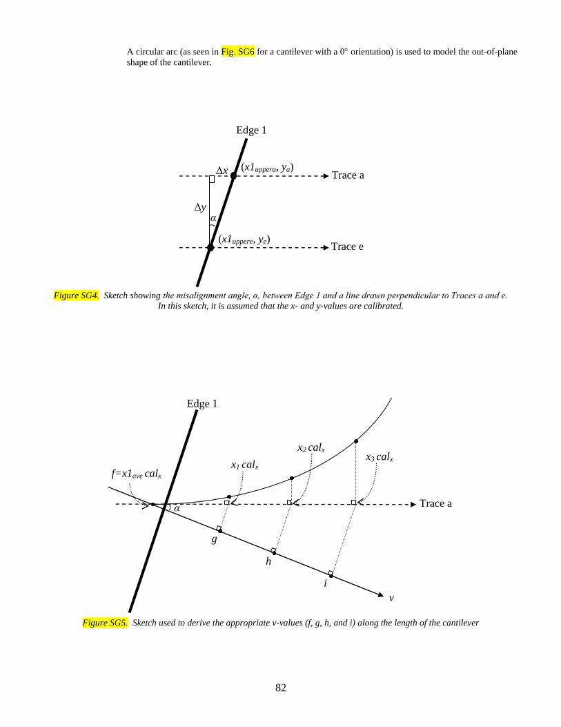
82

A circular arc (as seen in Fig. SG6 for a cantilever with a 0 orientation) is used to model the out-of-plane

shape of the cantilever.

Figure SG4. Sketch showing the misalignment angle, α, between Edge 1 and a line drawn perpendicular to Traces a and e.

In this sketch, it is assumed that the x- and y-values are calibrated.

Figure SG5. Sketch used to derive the appropriate v-values (f, g, h, and i) along the length of the cantilever

Trace a

Edge 1

α

Δx

Trace e

Δy

(x1uppera, ya)

(x1uppere, ye)

Trace a

Edge 1

g

h

i

x2 calx

x1 calx

α

f=x1ave calx

x3 calx

v

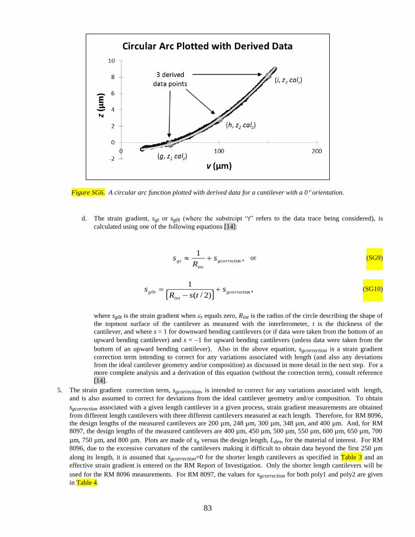
83

Figure SG6. A circular arc function plotted with derived data for a cantilever with a 0 orientation.

d. The strain gradient, sgt or sg0t (where the substrcipt “t” refers to the data trace being considered), is

calculated using one of the following equations [14]:

,1

ngcorrectio

int

gt sR

s or (SG9)

,

)2/(

1ngcorrectio

int

0tg stsR

s

(SG10)

where sg0t is the strain gradient when r equals zero, Rint is the radius of the circle describing the shape of

the topmost surface of the cantilever as measured with the interferometer, t is the thickness of the

cantilever, and where s = 1 for downward bending cantilevers (or if data were taken from the bottom of an

upward bending cantilever) and s = 1 for upward bending cantilevers (unless data were taken from the

bottom of an upward bending cantilever). Also in the above equation, sgcorrection is a strain gradient

correction term intending to correct for any variations associated with length (and also any deviations

from the ideal cantilever geometry and/or composition) as discussed in more detail in the next step. For a

more complete analysis and a derivation of this equation (without the correction term), consult reference

[14].

5. The strain gradient correction term, sgcorrection, is intended to correct for any variations associated with length,

and is also assumed to correct for deviations from the ideal cantilever geometry and/or composition. To obtain

sgcorrection associated with a given length cantilever in a given process, strain gradient measurements are obtained

from different length cantilevers with three different cantilevers measured at each length. Therefore, for RM 8096,

the design lengths of the measured cantilevers are 200 µm, 248 µm, 300 µm, 348 µm, and 400 µm. And, for RM

8097, the design lengths of the measured cantilevers are 400 µm, 450 µm, 500 µm, 550 µm, 600 µm, 650 µm, 700

µm, 750 µm, and 800 µm. Plots are made of sg versus the design length, Ldes, for the material of interest. For RM

8096, due to the excessive curvature of the cantilevers making it difficult to obtain data beyond the first 250 µm

along its length, it is assumed that sgcorrection=0 for the shorter length cantilevers as specified in Table 3 and an

effective strain gradient is entered on the RM Report of Investigation. Only the shorter length cantilevers will be

used for the RM 8096 measurements. For RM 8097, the values for sgcorrection for both poly1 and poly2 are given

in Table 4.

84

6. The resulting strain gradient value, sg, is the average of the strain gradient values obtained from Traces b, c, and d

as given below:

.3

gdgcgb

g

ssss

(SG11)

4.4 Strain Gradient Uncertainty Analysis

In this section, uncertainty equations are presented for use with strain gradient. The first uncertainty equation (presented in Sec.

4.4.1) is used for the MEMS 5-in-1. The equations used in the round robin experiment and other previous work are presented in

Sec. 4.4.2.

4.4.1 Strain Gradient Uncertainty Analysis for the MEMS 5-in-1

For the MEMS 5-in-1, the combined standard uncertainty, ucsg3, for strain gradient measurements with twelve uncertainty


2

)(

222

2

)(

2222222

samprepeatcorrectionlineardrift

shsrepeatcertnoiseRavexresxcalzresW

3csguuuu

uuuuuuuuu

, (SG12)

with additional sources of uncertainty considered negligible. A number following the subscript “sg” in “ucsg” indicates the data

analysis sheet that is used to obtain the combined standard uncertainty value. Therefore, ucsg3 implies that Data Analysis Sheet

SG.3 [3,13] is used.

In Eq. (SG12), uW is the uncertainty due to variations across the width of the beam, uzres is the uncertainty due to the resolution

of the interferometer in the z-direction, uxcal is the uncertainty due to the calibration in the x-direction, and uxres is the

uncertainty due to the resolution of the interferometric microscope in the x-direction. Next, uRave is the uncertainty due to the

sample’s surface roughness, unoise is the uncertainty due to interferometric noise, ucert is due to the uncertainty of the value of

the physical step height standard, urepeat(shs) is the uncertainty due to the repeatability of a measurement taken on the physical

step height standard, udrift is the uncertainty due to the amount of drift during the data session, and ulinear is the uncertainty due

to the deviation from linearity of the data scan. Then, in Eq. (SG12), ucorrection is the uncertainty in the strain gradient

correction term due to geometry and/or composition deviations from the ideal cantilever and urepeat(samp) is the uncertainty of

strain gradient repeatability measurements taken on cantilevers processed similarly to the one being measured.

With a few variations, the combined standard uncertainty equations and the calculations for each uncertainty component are

similar to those presented for residual strain measurements. Therefore, refer to Sec. 3.4.1 for the general approach. More

specifically, refer to Tables SG2, SG3, SG4, and SG5 where mention is made of Tables RS2, RS3, RS4, and RS5, respectively.

In addition, replace the words “residual strain” with the words “strain gradient,” replace “fixed-fixed beams” with “cantilevers,”

replace r-low with sg-low, r-high with sg-high, zxx with zx, and replace Eq. (RS23), Eq. (RS24), and Eq. (RS25) with Eq. (SG12),

Eq. (SG13), and Eq. (SG14), respectively, where:

lin1xlinear zzzz )( (where zx and z1 are considered calibrated values for this discussion), and (SG13)

gtsamprepeattsamprepeat su )()( . (SG14)


statistical Type A analysis) is used for each source of uncertainty, except where noted in Table SG2.

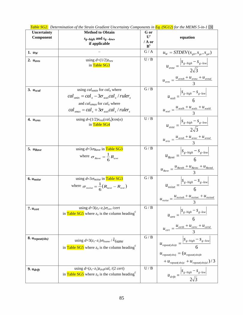
85

Table SG2. Determination of the Strain Gradient Uncertainty Components in Eq. (SG12) for the MEMS 5-in-1 [3]

Uncertainty

Component

Method to Obtain

sghigh and sglow, if applicable

G or

Ua

/ A or

Bb

equation

1. uW – G / A ),,( gdgcgbW sssSTDEVu


in Table SG3

U / B

32

lowghighg

zrest

ssu

3

zresdzresczresb

zres

uuuu





G / B

6

lowghighg

xcalt

ssu

3

xcaldxcalcxcalb

xcal

uuuu

4. uxres using d(1/2)xres(calx)cos(α)

in Table SG4

U / B

32

lowghighg

xrest

ssu

3

xresdxrescxresb

xres

uuuu

5. uRave using d=3Rave in Table SG3

where aveRave R

6

1

G / B

6

lowghighg

Ravet

ssu

3

RavedRavecRaveb

Rave

uuuu

6. unoise using d3noise in Table SG3

where avetavenoise RR 6

1

G / B

6

lowghighg

noiset

ssu

3

sec noisednoinoiseb

noise

uuuu

7. ucert using d=3(zxz1)cert/cert

in Table SG5 where zx is the column headingc

G / B

6

lowghighg

certt

ssu

3

certdcertccertb

cert

uuuu

8. urepeat(shs) using d=3(zxz1)6same/ samez6


G / B

6)(

lowghighg

tshsrepeat

ssu

bshsrepeatshsrepeat uu )()( (

3/))()( dshsrepeatcshsrepeat uu

9. udrift using d=(zxz1)zdriftcalz/(2 cert)


U / B

32

lowghighg

driftt

ssu

86

3

driftddriftcdriftb

drift

uuuu

10. ulinear using d=zlinear

in Table SG5

U / B

32

lowghighg

lineart

ssu

3

lineardlinearclinearb

linear

uuuu

11. ucorrection – G / B tcorrectioncorrection uu

3/ngcorrectios

12. urepeat(samp) – G / A gtsamprepeattsamprepeat su )()(

bsamprepeatsamprepeat uu )()( (

3/))()( dsamprepeatcsamprepeat uu



c For ease of presentation, zx and z1 in this table are considered calibrated. (Actually, these values are uncalibrated as presented earlier

in this SP 260. Therefore, the uncalibrated values should be multiplied by calz before use in this table.)

Table SG3. Three Sets of Inputsa for Strain Gradient Calculations to Determine uzrest, uRavet, unoiset, and usamp

b

z1 z2 z3

1 z1 z2 z3

2 z1+d z2d z3+d

3 z1d z2+d z3d a For ease of presentation, the values for z1, z2, and z3 in this table are assumed

to be calibrated. b

In this table, d=(1/2)zres to determine uzrest, d=3Rave to determine uRavet,

d=3noise to determine unoiset, and in Sec. 4.4.2 d=3samp to determine usamp.

Table SG4. Seven Sets of Inputsa for Strain Gradient Calculations to Determine uxrest

g h i

1 g h i

2 g + d h i d

3 g d h i + d

4 g + d h + d i d

5 g + d h d i d

6 g d h + d i + d

7 g d h d i + d a

In this table, d=(1/2)xres(calx)cos(α).

87

Table SG5. Three Sets of Inputsa for Strain Gradient Calculations

to Determine ucertt, urepeat(shs)t, udriftt, ulineart, and uzcal b

z1 z2 z3

1 z1 z2 z3

2 z1 z2+d z3+d

3 z1 z2d z3d a

For ease of presentation, the values for z1, z2, and z3 are assumed to be calibrated

in this table and in the applicable equations for d. b

In this table, d=3(zxz1)cert/cert to determine ucertt where zx is the column heading,

d=3(zxz1)6same/ same6z

to determine urepeat(shs)t, d=(zxz1)zdrift calz/(2 cert) to

determine udriftt, d=zlinear to determine ulineart, and in Sec. 4.4.2 d=3(zxz1)zcal/cert

to determine uzcal.

The expanded uncertainty for strain gradient, Usg, is calculated using the following equation:

3csg3csgsg ukuU 2 , (SG15)



Gaussianly distributed with approximate combined standard uncertainty ucsg3, the strain gradient is believed to lie in the interval

sg ucsg3 (expansion factor k=1) representing a level of confidence of approximately 68 %.

4.4.2 Previous Strain Gradient Uncertainty Analyses

In this section, two uncertainty equations are presented; one that was used in the round robin experiment and one that was used

before Eq. (SG12). For these equations, the strain gradient is assumed to be the strain gradient value obtained from Trace c

without a correction term and it is assumed that α = 0.

The uncertainty equation used in the round robin experiment uses six sources of uncertainty with all other sources of uncertainty

considered negligible. This strain gradient uncertainty equation (as calculated in Data Analysis Sheet SG.1 [13] and in ASTM

standard test method E 2246-05 [41]) with six sources of uncertainty is as follows:

222222

xresxcalzcalsampzresW1csg uuuuuuu . (SG16)

A number following the subscript “sg” in “ucsg” indicates the data analysis sheet that is used to obtain the combined standard

uncertainty value. Therefore, ucsg1 implies that Data Analysis Sheet SG.1 is used. In Eq. (SG16), uW, uzres, uxcal, and uxres are

defined in Sec. 4.4.1. Also in the above equation, usamp is the uncertainty due to the sample’s peak-to-valley surface roughness

as measured with the interferometer, and uzcal is the uncertainty of the calibration in the z-direction. These six uncertainty

components are calculated as specified in Sec. 3.4.2, replacing the words “residual strain” with the words “strain gradient,”

“fixed-fixed beams” with “cantilevers,” r-low with sg-low, and r-high with sg-high. In addition, refer to Tables SG2, SG3, SG4,

SG5, and SG6 where mention is made of Tables RS2, RS3, RS4, RS5, and RS6, respectively.

88

Table SG6. Determination of Some Strain Gradient Uncertainty Components in Eq. (SG16) and Eq. (SG17) [11,41]

Uncertainty

Component

Method to Obtain

sghigh and sglow

G or Ua

/ A or Bb

equation

1. uW using Trace b,

Trace c, and Trace d

U / B

32

lowghighg

W

ssu


in Table SG3

U / B

32

lowghighg

zres

ssu

3. usamp using d3samp

in Table SG3

G / B

6

lowghighg

samp

ssu

4. uzcal using d=3(zxz1)zcal/cert


G / B

6

lowghighg

zcal

ssu





G / B

6

lowghighg

xcal

ssu

6. uxres using d(1/2)xres(calx)

in Table SG4

U / B

32

lowghighg

xres

ssu

7. urepeat(shs) using d=(zxz1)zrepeat(shs)/(2 6z )


U / B

32)(

lowghighg

shsrepeat

ssu



c For ease of presentation, zx and z1 in this table are considered calibrated. (Actually, these values are uncalibrated as presented earlier

in this SP 260, therefore, the uncalibrated values should be multiplied by calz before use in this table.)


statistical Type A analysis) is used for each source of uncertainty. Table SG7 gives example values for each of these uncertainty

components as well as the combined standard uncertainty value, ucsg1.

89

Table SG7. Example Strain Gradient Uncertainty Valuesa

From a Round Robin Surface-Micromachined Chip

source of uncertainty or descriptor uncertainty value

(m1

)

1. uW variations across the width of the beam 0.186

2. uzres interferometric resolution in z-direction 0.037

3. usamp interferometric peak-to-valley surface roughness 0.423

4. uzcal calibration in z-direction 0.012

5. uxcal calibration in x-direction 0.013

6. uxres interferometric resolution in x-direction 0.056

ucsg1b combined standard uncertainty for strain gradient 0.467

a As determined in ASTM standard test method E 2246-05 [41] using Eq. (SG16) for a cantilever with a design length of 550 m and with

a 0 orientation. b This value for ucsg1 was used in the round robin (see Sec. 4.5) and is incorporated into the calculations of ucsg1ave as presented in the

sixth row of Table SG8, which uses Eq. (SG16).

An expanded version of the uncertainty calculation presented in Eq. (SG16) is given below, which includes ten sources of

uncertainty:

222

)(

2222222

lineardriftshsrepeatcertnoiseRavexresxcalzresW2csg uuuuuuuuuuu . (SG17)

This calculation is done using Data Analysis Sheet SG.2 [13]. The first four components (uW, uzres, uxcal, and uxres) are

calculated as they are calculated for use in Eq. (SG16) using only Trace c. By using the above equation [instead of Eq. (SG16)],

the z-calibration procedures are the same for the different applicable measurements in this SP 260 for the MEMS 5-in-1 RMs

[by using a procedure such as given in Sec. 5.2 for step height measurements (as used with the MEMS 5-in-1) as opposed to the

method referred to in Sec. 4.2 for earlier versions]. Therefore, the component, uzcal in Eq. (SG16) gets replaced with the

components ucert, udrift, and ulinear as described in Sec. 3.4.1 (after making the appropriate substitutions and using only the data

from Trace c) and with the component urepeat(shs) as described in Sec. 3.4.2 (after making the appropriate substitutions). Also,

to provide more physical understanding to the resulting uncertainties, the uncertainty component usamp in Eq. (SG16) is replaced

with the components uRave and unoise in Eq. (SG17). These two components are described in Sec. 3.4.1 (after making the

appropriate substitutions and using only the data from Trace c).

4.5 Strain Gradient Round Robin Results

The MEMS Length and Strain Round Robin repeatability and reproducibility results are given in this section for strain gradient

measurements. The repeatability data were taken in one laboratory using an optical interferometer (see Sec. 1.1.2). Unlike the

MEMS 5-in-1 chips shown in Figs. 2(a and b) for RM 8097, a similarly processed surface-micromachined test chip (from

MUMPs46 [9] and without the backside etch) was fabricated on which strain gradient measurements were taken from poly1

cantilever test structures having a 0 orientation and from poly1 cantilevers having a 90 orientation. An array of the cantilevers

on the round robin test chip with a 0˚ orientation is shown in Fig. SG7. Each cantilever array has design lengths from 400 m to

800 m, inclusive, in 50 m increments. (All the cantilevers are 10 m wide.) However, only the design lengths between 400

m to 750 m, inclusive, were used in obtaining the repeatability data. Therefore, with three beams designed at each length, 48

measurements were taken (24 measurements at each orientation). See Fig. SG8(a) for a design rendition of a poly1 cantilever

on the round robin test chip and Figs. SG8(b and c) for applicable 2D data traces taken from this cantilever.

90

Figure SG7. An array of cantilevers on the round robin test chip.

(a)

(b)

00.5

11.5

22.5

33.5

44.5

5

0.1 0.3 0.5 0.7 0.9 1.1

z(u

m)

x (mm)

Data along Trace a or e

Edge 1

x1upper

x1lower

a

e

L

Edge 1 Edge 2

poly0

poly1


y

x c d

b

Edge 3

y

x

91

(c)

012345678

0.1 0.3 0.5 0.7 0.9 1.1

z(µ

m)

x (mm)


Edge 2

Edge 3

Figure SG8. For a cantilever test structure on the round robin test chip, (a) a design rendition,

(b) an example of a 2D data trace used to locate the attachment point of the cantilever in (a),

and (c) an example of a 2D data trace taken along the length of the cantilever in (a).

For the reproducibility data,40

a round robin test chip was passed from laboratory to laboratory. Each participant was asked to

obtain a strain gradient measurement from two poly1 cantilevers in an array, such as shown in Fig. SG7, that had either a 0

orientation or a 90 orientation. One of the cantilevers was requested to have a design length of 650 m. The design length for

the other cantilever could range from 500 m to 650 m, inclusive. The results from one of the two cantilevers is presented

below. Following the 2002 version of ASTM standard test method E 2246 [42] for strain gradient measurements, the raw,

uncalibrated measurements were recorded on Data Analysis Sheet H (similar to the existing Data Analysis Sheet SG.1 [13]) for

measurements of strain gradient.

Table SG8 presents the strain gradient repeatability and reproducibility results. In this table, n is the number of measurements

followed by the average of the repeatability or reproducibility measurement results (namely, sgave). For the repeatability

measurements only, repeat(samp) is given, which is the relative standard deviation of the repeatability strain gradient

measurements. Then, the ±2σsg limits are given, where σsg is the standard deviation of the strain gradient measurements,

followed by the average of the repeatability or reproducibility combined standard uncertainty values (i.e., ucsgave) for different

calculations.

40

Between-laboratory variability pertains to test results obtained in different laboratories on random test units from the same lot of

homogeneous material

92

Table SG8. Strain Gradient Measurement Results


Ldes= 500 m to 650 m



Reproducibility results


1. n 24 48 6

2. sgave 4.71 m1

4.97 m1

4.67 m1

repeat(samp) 13 % 20 %

4. ±2σsg limits ±1.2 m

1

(± 25 %)

±2.0 m1

(± 40 %)

±1.7 m1

(± 37 %)

5. ucsg1avea 0.73 m

1

(14 %)

0.84 m1

(17 %)

0.56 m1

(12 %)

6. ucsg1aveb

0.47 m1

(10 %)

0.56 m1

(11 %)

7. ucsg2avec 0.44 m

1

(9.5 %)

0.52 m1

(11 %)

8. ucsg3aved 0.74 m

1

(16 %)

1.12 m1

(23 %)

a Where ucsg1 is determined in ASTM standard test method E 224602 [42]. For this calculation, the usamp and uzcal components

in the ucsg1 calculation in Eq. (SG16) are combined into one component. For this component, assuming a uniform (that is, rectangular)

probability distribution, the limits are represented by a 20 nm variation in the z-value of the data points. Also, in ASTM standard

test method E 224602, uzres=uxcal=uxres=0 m1

. b Where ucsg1 is determined in ASTM standard test method E 224605 [41] using Eq. (SG16).

c Where ucsg2 is determined using Eq. (SG17).

d Where ucsg3 is determined using Eq. (SG12).

Comments concerning the round robin data include the following:

a) Plots: In this round robin, random length cantilevers were measured. As such, there are at least two variables

(orientation and length) as discussed below.

i) Orientation: Figure SG9 is a plot of sg versus orientation, which reveals no obvious orientation dependence.

ii) Length: Figure SG10 is a plot of sg versus design length, where the data indicate a decrease in the strain gradient

for increasing length (for Ldes = 400 m to 600 m) that levels off (from Ldes=600 m to 750 m).

Figure SG9. A plot of sg versus orientation41

.

41



sgavex=5.05 m1

±2σsg limits = ±40 % sgavey = 4.89 m

1

±2σsg limits = ±41 %

93

Figure SG10. A plot of sg versus length for two different orientations.42

b) Precision: The repeatability and reproducibility precision data appear in Table SG8. In particular, for the ±2σsg limits, the

repeatability data (i.e., ±25 %) are tighter than the reproducibility data (i.e., ±37 %) for the same span of design lengths. This is

due to the repeatability measurements being taken in the same laboratory using the same instrument by the same operator. It is

interesting to note that the ucsg1ave values for the repeatability measurements are slightly higher than the ucsg1ave values for the

reproducibility measurements.

c) Bias: No information can be presented on the bias of the procedure in ASTM standard test method E 2246 for measuring

strain gradient because there is not a certified MEMS material for this purpose.

4.6 Using the MEMS 5-in-1 to Verify Strain Gradient Measurements

To compare your in-house strain gradient measurements with NIST measurements, you will need to fill out Data Analysis Sheet

SG.3. (This data analysis sheet is accessible via the URL specified in the reference [13], a reproduction of which is given in


calculations, the data on the completed form can be compared with the data on the RM Report of Investigation and the


Calibrate the instrument: Calibrate the instrument as specified in Sec. 4.2 for RM measurements. Obtain the inputs for Table 1

in Data Analysis Sheet SG.3.

Locate the cantilever: In the third grouping of test structures, shown in Figs. SG1(a, b, and c), on the MEMS 5-in-1 chips

shown in Fig. 1 and Figs. 2(a and b) for RM 8096 and RM 8097 (fabricated on MUMPs98 and MUMPs95), strain gradient

measurements are made. Cantilever test structures are provided for this purpose, as shown in Fig. SG2(a) for RM 8096 and as

shown in Fig. SG3(a) for the poly2 cantilevers on RM 8097 (fabricated on MUMPs95). Data Analysis Sheet SG.3 requires

measurements from one cantilever test structure. The specific test structure to be measured can be deduced from the data

entered on the NIST-supplied Data Analysis Sheet SG.3 that accompanies the RM.

For the strain gradient grouping of test structures for RM 8096, as shown in Fig. SG1(a), the target test structure can be found as

follows:

1. The input design length (i.e., input #4 on Data Analysis Sheet SG.3, a reproduction of which is given in Appendix

3) specifies the design length of the cantilever. The design length of the cantilever (in micrometers) is given at the

top of each column of test structures in Fig. SG1(a) following the column number (i.e., 1 to 5), therefore design

length can be used to locate the column in which the target test structure resides. Design lengths for the cantilever

test structures are given in Table SG1.

2. The input which cantilever (i.e., input #6) specifies which cantilever in the column to measure (i.e., the “first,”

42

Ibid.

sgave=4.26 m1


sgave=4.24 m1


sgave=5.71 m1


94

“second,” “third,” etc.) regardless of the orientation.

3. The input orientation (i.e., input #8) can be used as a form of verification. The cantilevers are designed at both a 0

and a 180 orientation with the cantilevers having a 0 orientation being the first, second, and third cantilevers in

each column and the cantilevers with a 180 orientation being the fourth, fifth, and sixth cantilevers in each column.

Therefore, either 0 or 180 will be selected for orientation.

For the strain gradient grouping of test structures for RM 8097 (fabricated on MUMPs98 and MUMPs95), as shown in Figs.

SG1(b and c), respectively, the target test structure can be found as follows:

1. The input material (i.e., input #3) is used to identify if a cantilever in a poly1 array is to be measured or if a

cantilever in a poly2 array is to be measured. The two poly1 arrays in Figs. SG1(b and c) have a P1 designation and

the one poly2 array has a P2 designation.

2. The input orientation (i.e., input #8) specifies the orientation of the cantilever array. The cantilevers in the lower

left poly1 array have a 180 orientation and the cantilevers in the upper poly1 array have a 90 orientation. The

poly2 array has a 180 orientation.

3. The input design length (i.e., input #4) specifies the design length of the cantilever. The design length of the

cantilever (in micrometers) is given next to the second of three cantilevers of the same length, as can barely be seen

in Figs. SG1(b and c). Therefore, design length can be used to locate a set of three possible target test structures.

Design lengths for the cantilever test structures are given in Table SG1.

4. The input which cantilever (i.e., input #6) specifies which cantilever in the set of three possible target test structures

of the same length in the array to measure (i.e., the “first,” “second,” “third,” etc.). Since there are three instances of

each test structure, the radio button corresponding to “first,” “second,” or “third” is used to identify the target test

structure.

Take the measurements: Following the steps in ASTM standard test method E 2246 [3] for strain gradient measurements, the

chip is oriented under the interferometric optics as shown in Fig. SG2(a) or Fig. SG3(a)43

and one 3-D data set is obtained using

typically the highest magnification objective that is available and feasible. The data are leveled and zeroed, and Traces a, b, c,

d, and e are obtained. Traces a and e are used to calculate the misalignment angle, α. From Traces a and e, measurements of

xupper and nt (typically from Edge 1) are entered into Data Analysis Sheet SG.3. The uncalibrated values for ya and ye are also

recorded.

For RM 8096, with Data Analysis Sheet SG.3, uncalibrated data points along the cantilever for (x1, z1), (x2, z2), and (x3, z3), are

requested from Traces b, c, and d, shown in Fig. SG2(c).

For RM 8097 (fabricated on MUMPs98 and MUMPs95), with Data Analysis Sheet SG.3, there are data restrictions due to

deviations from the ideal geometry of the cantilever as discussed in Sec. 4.1 and Sec. 4.3. In particular, uncalibrated data points

along the cantilever for (x1, z1), (x2, z2), and (x3, z3) are requested from Traces b, c, and d as shown in Fig. SG3(c) for a poly2

cantilever, and these data should be taken along the cantilever such that the uncalibrated x value of each data point is greater

than x6ave (assuming a 0 orientation of the cantilever).

Perform the calculations: Enter the data into Data Analysis Sheet SG.3 as follows:



2. Supply inputs to Table 1 through Table 3.

3. Press one of the “Calculate and Verify” buttons to obtain the results from the cantilever test structure. (One of these

buttons is located near the top of the data analysis sheet and the other is located near the middle of the data

analysis sheet.)







specifies a strain gradient value, sg, and the expanded uncertainty, Usg, (with k=2) intending to approximate a 95 % level of

confidence. It is your responsibility to determine an appropriate criterion for acceptance, such as given below:

43



95

22

)()( sgcustomersggcustomergsg UUssD , (SG18)

where Dsg is the absolute value of the difference between your strain gradient value, sg(customer), and the strain gradient value on

the RM Report of Investigation, sg, and where Usg(customer) is your expanded uncertainty value and Usg is the expanded

uncertainty on the RM Report of Investigation. If your measured value for strain gradient (as obtained in the newly filled out

Data Analysis Sheet SG.3) satisfies your criterion for acceptance and there are no pertinent “wait” statements at the bottom of

your Data Analysis Sheet SG.3, you can consider yourself to be appropriately measuring strain gradient according to the ASTM

E 2246 strain gradient standard test method [3] according to your criterion for acceptance.

An effective strain gradient value is reported for RM 8096, as shown in Fig. 1, due to deviations from the ideal geometry and/or

composition of the cantilever as discussed in Sec. 4.1 and Sec. 4.3. Most notably, the excessive curvature of the cantilevers on

this chip makes it difficult to obtain a strain gradient correction term, sgcorrection, as discussed in Sec. 4.3. When you use ASTM

standard test method E 2246 with your own cantilever, you must be cognizant of the geometry and composition of your

cantilever because this test method assumes an ideal geometry and composition, implying that you would be obtaining an

“effective” strain gradient value if the geometry and/or composition of your cantilever deviates from the ideal.



96

5 Grouping 4: Step Height A step height measurement is defined here as the distance in the z-direction between an initial, flat, processed surface (or

platform) and a final, flat, processed surface (or platform). These measurements can be used to determine thin film thickness

values (see Sec. 8), which are an aid in the design and fabrication of MEMS devices [31-32].

This section on step height supplements SEMI standard test method MS2 [4], which more completely presents the purpose,

scope, limitations, terminology, apparatus, and test structure design for MEMS as well as the calibration procedure,

measurement procedure, calculations, precision and accuracy, etc. In this section, the NIST-developed step height test

structures on RM 8096 and RM 8097 are described and illustrated in Sec. 5.1, the calibration procedure for step height

measurements is described in Sec. 5.2, the step height measurement procedure in Sec. 5.3, the uncertainty analysis in Sec. 5.4,

and the round robin results in Sec. 5.5. Section 5.6 describes how to use the MEMS 5-in-1 to verify step height measurements.

5.1 Step Height Test Structures

Step height measurements are taken in the fourth grouping of test structures, as shown in Fig. SH1(a) for RM 8096 depicted in

Fig. 1 in the Introduction and as shown in Fig. SH1(b) for RM 8097 depicted in Figs. 2(a and b).

(a)

(b)

Figure SH1. The step height grouping of test structures on (a) RM 8096, fabricated on a multi-user 1.5 m CMOS process

[8] followed by a bulk-micromachining etch, as depicted in Fig. 1 and (b) RM 8097, fabricated using a polysilicon multi-user

surface-micromachining MEMS process [9] with a backside etch, as depicted in Figs. 2(a and b).

A step height test structure from each of the groupings shown in Fig. SH1 is given in Fig. SH2(a) and Fig. SH3(a), respectively.

y

x

y

x

97

(a)

(b)

(c)

Figure SH2. For a step height test structure on RM 8096 as shown in Fig. 1, (a) a design rendition,

(b) a cross section, and (c) an example of a 2D data trace from (a).

98

(a)

(b)

(c)

Figure SH3. For a step height test structure on RM 8097 as shown in Figs. 2(a and b), (a) a design rendition,

(b) a cross section, and (c) an example of a 2D data trace from (a).

The step height test structures on RM 8096 and RM 8097 are described below.

For RM 8096: In the grouping of step height test structures given in Fig. SH1(a) for RM 8096, there are four distinct test

structures (with three rows of each structure) for which six step height transitions are indicated by arrows above the topmost test

structure in the row. We will only be concerned with those steps associated with an arrow. For the MEMS 5-in-1, only one

occurrence of one of these six step heights is used to obtain the reference value for step height.

The six step height measurements in this grouping of test structures can be used to calculate the composite beam oxide thickness

(for Young’s modulus calculations). It is important to keep in mind that the fourth test structure (associated with the fifth and

99

sixth arrows) does not have a reflective top surface for each platform and as such is intended to be used with a stylus instrument.

Consult Sec. 8 for details concerning this as well as the cross sections of each of the test structures given in Fig. SH1(a).

The approximate design dimensions of the four test structures in Fig. SH1(a) are given in Table SH1.

Table SH1. Design Dimensions (in Micrometers) as Depicted in Fig. SH4

For the Step Height Test Structures in Fig. SH1(a) For RM 8096

First Test

Structure

Second Test

Structure

Third Test

Structure

Fourth Test

Structure

w 150 150 150 150

l 50 50 100 100

r 94 94 94 94

Figure SH4. A step height test structure depicted in Fig. SH1(a).

For RM 8097: In the grouping of step height test structures given in Fig. SH1(b) for RM 8097, the step height test structures are

grouped in quads. The second quad (as indicated by the number “2” in the center of the quad) is shown in Fig. SH5. There are

four step height test structures within each quad, each with a different orientation. The upper left test structure has a 0

orientation, the bottom left has a 90 orientation, the bottom right has a 180 orientation and the upper right has a 270

orientation. Each of the test structures is a step from the top of the polysilicon layer called “poly1” or “p1” to the top of the

polysilicon layer called “poly2” or “p2,” or vice versa. In Fig. SH5, the “P1” and “P2” labels closest to the platform in the step

can be used to determine which platform is made of poly1 and which is made of poly2. The design layer for the surrounding

reference platform is called “poly0” or “p0.”

Figure SH5. Quad 2 in the step height grouping depicted in Fig. SH1(b).

There are two different sized quads in the step height grouping in Fig. SH1(b). The larger fourth and fifth quads are intended

for use with a stylus instrument, although an optical instrument can also be used. The approximate design dimensions for the

test structures in the two different sized quads are given in Table SH2, which refers to the labeling in Fig. SH6. As can be seen

p0

p1

p2

100

in Fig. SH6, the platform dimensions (including the anchor dimensions as given by the subscript “a”) for Platform A and

Platform B are the same.

Table SH2. Design Dimensions (in Micrometers) as Depicted in Fig. SH6

For the Step Height Test Structures in Fig. SH1(b) For RM 8097

For test structures in

Quads 1, 2, and 3

For test structures in

Quads 4 and 5

l w 60 110 110 160

la wa 50 100 100 150

r 100 100

R1 325 425

R2 310 360

Figure SH6. A step height test structure depicted in Fig. SH1(b).

5.2 Calibration Procedures for Step Height Measurements

For step height measurements, the optical interferometer (or comparable instrument) is calibrated in the z-direction. The

calibration procedure used with the MEMS 5-in-1 [4] is given below followed by the calibration procedure used when

discussing earlier versions of the step height uncertainty equation presented in Sec. 5.4.

Calibration in the z-direction (as used with the MEMS 5-in-1) [4]:

1. Use the same “slope” value, if applicable, as obtained in Sec. 1.1.2.2. Verify that this slope value is adequate by

using the instrument’s prescribed calibration procedure to make sure that the difference between the instrument’s

step height measurements on a physical step height standard and the certified value of the physical step height

standard is less than or equal to 1 %. If it is not, recalibrate the instrument to obtain a new “slope” value or

perform the steps in Sec. 1.1.2.2 to validate the step height measurements.

2. Before the data session:

a. The height of the physical step height standard is recorded at six locations.

i. If single-sided step height measurements are taken, the six measurements are taken with three

measurements spread out evenly along each side of the physical step height standard. (The

101

measurements are taken within the specified certified area along the length and width of the

step.44

)

ii. If double-sided step height measurements are taken, the six measurements are spread out evenly

along the certified area of the physical step height standard.

The mean value of the six measurements is called beforez . The standard deviation of these six

measurements is called σbefore.

b. In addition, six step height measurements are taken at the same location on the physical step height

standard. (This location is within the specified certified area along the length and width of the step.) The

mean value of the six measurements taken at the same location is called same1z . The standard deviation

of these six measurements is called σsame1.

3. Similarly, after the data session:

a. The height of the physical step height standard is recorded at six locations.

i. If single-sided step height measurements are taken, the six measurements are taken with three

measurements spread out evenly along each side of the physical step height standard. (The

measurements are taken within the specified certified area along the length and width of the

step.)

ii. If double-sided step height measurements are taken, the six measurements are spread out evenly

along the certified area of the physical step height standard.

The mean value of the six measurements is called afterz . The standard deviation of these six

measurements is called σafter.

b. In addition, six step height measurements are taken at the same location on the physical step height

standard as before the data session. The mean value of the six measurements taken at the same location is

called same2z . The standard deviation of these six measurements is called σsame2.

[Note that if it can be demonstrated that a given instrument does not drift significantly during a data session, this

second step can be skipped and it can be assumed that afterbefore zz , σbefore = σafter, same2same1 zz , and σsame1

= σsame2.

4. The average of the calibration measurements, avez , is calculated using the following formula:

2

afterbefore

ave

zzz

. (SH1)

5. The z-calibration factor for the instrument, calz, is determined using the following equation:

ave

zz

certcal , (SH2)

where cert is the certified value of the physical step height standard. The z-data values obtained during the data

session are multiplied by calz to obtain calibrated z-data values.

6. For uncertainty calculations, the quantities, cert and zlin, are recorded where cert is the certified uncertainty

of the physical step height standard and zlin is the maximum relative deviation from linearity over the total scan

range of the instrument (as quoted by the manufacturer or as determined in Sec. 1.1.2.2). Also, zdrift, σ6ave, 6avez ,

σ6same, and 6samez (as defined in the Definition of Symbols Section)

45 are determined as follows:

44

The location of the certified area should be indicated in the Certificate accompanying the physical step height standard. Please note that the area close to the

step transition is typically not included in the certified region. 45

The values for zdrift, σ6ave, ,6ave

z σ6same, and samez

6 as calculated here are uncalibrated to match the inputs to Data Analysis Sheet SH.1.a .

102

2same1samedrift zzz , (SH3)

if afterbefore , then before6ave and before6ave zz , (SH4)

if afterbefore , then after6ave and after6ave zz , (SH5)

if same2same1 , then 1same6same and 1same6same zz , and (SH6)

if same2same1 , then 2same6same and 2same6same zz . (SH7)

Calibration in the z-direction (for discussing earlier versions of the step height uncertainty equations) [43,44]: The following

measurements are taken on a calibrated double-sided physical step height standard:

1. Before the data session, six step height measurements are taken at the same location on the physical step height

standard. This location is within the specified certified area along the length and width of the step46

of the

standard. The mean value of the six measurements taken at the same location is called 1amesz . The minimum

of the six measurements is called zmin1. The maximum is called zmax1.

2. Similarly, after the data session, six step height measurements are taken on the physical step height standard at the

same location as before the data session. The mean value of these six meaurements is called 2samez . The

minimum of the six measurements is called zmin2. The maximum is called zmax2. [Note that if it can be

demonstrated that a given instrument does not drift significantly during a data session, this step can be skipped and

it can be assumed that ,1same2same zz ,min1min2 zz and .max1max2 zz ]

3. The average of the calibration measurements, samez , is calculated using the following formula:

2

2same1samesame

zzz

. (SH8)

4. The z-calibration factor for the instrument, calz, is determined using the following equation:

same

zz

certcal , (SH9)

where cert is the certified value of the physical step height standard. The z-data values obtained during the data

session are multiplied by calz to obtain calibrated z-data values.

5. For uncertainty calculations, the quantities, cert and zperc, are recorded where cert is the combined standard

uncertainty of the calibrated physical step height standard and zperc (also called zlin) is the maximum relative

deviation from linearity over the total scan range of the instrument as quoted by the manufacturer. Also, zdrift,

zrepeat(shs), and 6z (as defined in the Definition of Symbols Section)47

are calculated using the following equations:

46

The location of the certified area should be indicated in the Certificate accompanying the physical step height standard. Please note that the area close to the

step transition is typically not included in the certified region.

47 The values for zdrift, zrepeat(shs), and 6

z as calculated here are uncalibrated to match the inputs to Data Analysis Sheet SH.1.

103

2same1samedrift zzz , (SH10)

min1max1)1repeat(shs zzz , (SH11)

min2max2)2repeat(shs zzz , (SH12)

if )2repeat(shs)1repeat(shs zz , then )1repeat(shs)repeat(shs zz and same1zz 6 , and (SH13)

if )2repeat(shs)1repeat(shs zz , then )2repeat(shs)repeat(shs zz and same2zz 6 . (SH14)

5.3 Step Height Measurement Procedure

For the MEMS 5-in-1, the step height measurements are taken from one step height test structure. Three 2D data traces [such

as, Trace a, Trace b, and Trace c, as shown in Fig. SH2(a) and Fig. SH3(a)] are taken along the top of the test structure, a cross

section of which is given in Fig. SH2(b) and Fig. SH3(b), respectively. Example 2D data traces are given in Fig. SH2(c) and

Fig. SH3(c), respectively. All height measurements are with respect to the height of the surrounding or partially surrounding

reference platform that is used to level and zero the data. For generic Test Structure N with platforms labelled X and Y, the

individual platform height measurements from Trace a, Trace b, and Trace c (namely, platNXa, platNXb, platNXc, platNYa,

platNYb, and platNYc) and the standard deviations from the two platforms associated with the step (namely, splatNXa, splatNXb,

splatNXc, splatNYa, splatNYb, and splatNYc) are recorded,48

being careful to extract these measurements from portions not close to the

transitional edges. If the test structure in Fig. SH2(a) is called Test Structure 1, then for the step in Test Structure 1 from

Platform A to Platform B, as pointed to by the arrow above the step, the platform height measurements from Trace a, Trace b,

and Trace c would be plat1Aa, plat1Ab, plat1Ac, plat1Ba, plat1Bb, and plat1Bc and the standard deviations would be splat1Aa,

splat1Ab, splat1Ac, splat1Ba, splat1Bb, and splat1Bc.49

Therefore, from the three profiles, twelve parameters (including both step

heights and standard deviations) are obtained (six from Platform A and six from Platform B).

The step height from each profile (in general, stepNXYt)50

is given by:

zXYt calplatNXtplatNYtstepN , (SH15)

where t is the data trace (a, b, c, etc.) being examined. For the step indicated by the arrow shown in Fig. SH2(a) from Platform

A to Platform B, the equations are:

zABa calAa1platBa1plat1step , (SH16)

zABb calAb1platBb1plat1step , and (SH17)

zABc calAc1platBc1plat1step . (SH18)

The step height, stepNXY, is the average of the values from the different surface profiles as given below:

48

Consult the Definition of Symbols Section for the nomenclature used for platNXt and splatNXt. 49

These are uncalibrated values to match the inputs to Data Analysis Sheet SH.1.a. 50

Consult the Definition of Symbols Section.

104

3

XYcXYbXYaXY

stepNstepNstepNstepN

. (SH19)

For the step shown in Fig. SH2(a), the step height, step1AB, is:

3

ABcABbABaAB

1step1step1step1step

. (SH20)

The calculation of the combined standard uncertainty, ucSH, for stepNXY is described next.

5.4 Step Height Uncertainty Analysis

In this section, uncertainty equations are presented for use with step height. The first uncertainty equation (presented in Sec.

5.4.1) is used with the MEMS 5-in-1 [4]. An earlier equation [43] used in the round robin experiment is presented in Sec. 5.4.2.

5.4.1 Step Height Uncertainty Analysis for the MEMS 5-in-1

For the MEMS 5-in-1, the combined standard uncertainty, ucSH1a, for step height measurements with eight uncertainty


2

)(

222

)(

2222

samprepeatlineardriftshsrepeatcalcertWstepLstep1acSH uuuuuuuuu , (SH21)

where a number or a number and a letter following the subscript “SH” in “ucSH” indicates the data analysis sheet that is used to

obtain the combined standard uncertainty value. Therefore, ucSH1a implies that Data Analysis Sheet SH.1.a [4,13] is used. In

this equation,

uLstep is the uncertainty of the measurement across the length of the step where the length is measured perpendicular to

the edge of the step,51

uWstep is the variation in measured step height values sampled across the width of the step,

ucert is the uncertainty of the value of the physical step height standard used for calibration,

ucal is the uncertainty of the measurements taken across the physical step height standard,

urepeat(shs) is due to the repeatability of measurements on the physical step height standard,

udrift is the uncertainty due to the amount of drift during the data session,

ulinear is the uncertainty of a measurement due to the deviation from height linearity of the data scan, and

urepeat(samp) is the uncertainty of step height repeatability measurements taken on test structures processed similarly to

the one being measured.

Table SH3 provides the equations for the uncertainty components. In determining the combined standard uncertainty, a Type B

evaluation [21-23] (i.e., one that uses means other than the statistical Type A analysis) is used for each source of uncertainty,

except where noted. This table can be referenced as each component is discussed.

The first uncertainty component in Eq. (SH21) and listed in Table SH3 is uLstep. This uncertainty is due to platforms that are not

level with respect to the reference platform, as seen in a surface profile. [Fig. SH2(c) is an example of such a profile.] To

estimate this component of uncertainty, the standard deviations along each platform in each surface profile are obtained (for

example, splat1Xa, splat1Xb, and splat1Xc for Platform X and splat1Ya, splat1Yb, and splat1Yc for Platform Y). For each platform, the

standard deviations from the different profiles are averaged together then calibrated as given in the following equations:

z

platNXcplatNXbplatNXa

platNXave calsss

s

3 and (SH22)

51

Stated differently, uLstep is the uncertainty in the step height due to the variation in the topography along each platform (that is not due to roughness).

105

z

platNYcplatNYbplatNYa

platNYave calsss

s

3 . (SH23)

The equation for uLstep would then be obtained by adding splatNXave and splatNYave in quadrature. However, the fine scale

roughness (contained within the above standard deviations) should not be included in the uncertainty calculation of uLstep

because the roughness should not effect the step height value. For this analysis, the roughness is assumed to be the smallest of

all the standard deviations obtained for a given surface material. In other words, the roughnesses sroughNX and sroughNY are the

uncalibrated surface roughnesses of platNX and platNY, respectively, and are equated with the smallest of all the values obtained

for splatNXt and splatNYt, respectively, as given below:

),,(MIN platNXcplatNXbplatNXaroughNX ssss and (SH24)

),,(MIN platNYcplatNYbplatNYaroughNY ssss . (SH25)

However, if the surfaces of platNX, platNY, and platNr all have identical compositions, then sroughNX equals sroughNY, which

equals the smallest of all the values obtained for splatNXt, splatNYt, and splatNrDt.52

The square of each surface roughness is then

subtracted in the calculation of uLstep to obtain the equation given in the fourth column of Table SH3,53

which assumes a

Gaussian distribution.

Table SH3. Step Height Uncertainty Equations for the MEMS 5-in-1 [4,10]a

stepNXYmin and stepNXYmax G or Ub

/A or Bc

equation

1. uLstep G / B

])([

])([

22

22

zroughNYplatNYave

zroughNXplatNXave

Lstepcalss

calssu

2. uWstep G / A

),,( XYcXYbXYa

WstepWstep

stepNstepNstepNSTDEV

u

3. ucert G / B

XYcert

cert stepNcert

u

4. ucal G / A

XY

ave

avecal stepN

zu

6

6

5. urepeat(shs)

same

sameXYXYXY

zstepNstepNstepN

6

6min 3

same

sameXYXYXY

zstepNstepNstepN

6

6max 3

G / A

6

minmax)(

XYXYshsrepeat

stepNstepNu

XY

same

same stepNz6

6

6. udrift

cert

calzstepNstepNstepN

zdrift

XYXYXY2

min

cert

calzstepNstepNstepN

zdrift

XYXYXY2

max

U / B

32

minmax XYXYdrift

stepNstepNu

XY

zdriftstepN

cert

calz

32

52

Consult the Definition of Symbols Section as needed. 53

This equation is different than the one presented in [10].

106

7. ulinear linXYXYXY zstepNstepNstepN min

linXYXYXY zstepNstepNstepN max

U / B

32

minmax XYXYlinear

stepNstepNu

XYlin stepN

z

3

8. urepeat(samp) G / A XYsamprepeatsamprepeat stepNu )()(

a Refer to the Definition of Symbols Section as needed

b “G” indicates a Gaussian distribution and “U” indicates a uniform distribution

c Type A or Type B analysis

The uncertainty equation for uWstep is determined from Wstep, the calibrated one sigma standard deviation of the step height

measurements stepNXYa, stepNXYb, and stepNXYc, as given in the fourth column of Table SH3. This is a statistical Type A

component.

The uncertainty equation for ucert is determined from cert (the certified value of the double-sided physical step height standard

used for calibration) and cert (the certified one sigma uncertainty of the calibrated physical step height standard) as given in

Table SH3. The uncertainty of the measured step height is assumed to scale linearly with height. Therefore, ucert is calculated

using the equation given in Table SH3.

The uncertainty equation for ucal is determined from 6ave [the maximum of two uncalibrated values (σbefore and σafter)] and

avez6 (the uncalibrated average of the six calibration measurements from which 6ave is found) as given in Table SH3. The

uncertainty of the measured step height is assumed to scale linearly with height. Therefore, ucal is calculated using the equation

given in Table SH3.

The uncertainty equation for urepeat(shs) is determined from the minimum and maximum step height values (namely, stepNXYmin

and stepNXYmax, respectively) as given in Table SH3 where σ6same is the maximum of two uncalibrated values (σsame1 and

σsame2) and where samez6 is the uncalibrated average of the six calibration measurements from which σ6same is found. The

uncertainty of the measured step height is assumed to scale linearly with height. Assuming a Gaussian distribution (and

assuming uLstep, uWstep, ucert, ucal, udrift, ulinear, and urepeat(samp) equal zero), the value for stepNXY lies between stepNXYmin and

stepNXYmax. Therefore, urepeat(shs) is calculated using the equation given in Table SH3.54

In the same way, udrift is calculated (however a uniform distribution is assumed), resulting in the equation listed in Table SH3,

where zdrift is the uncalibrated positive difference between the averages of the six calibration measurements taken before and

after the data session (at the same location on the physical step height standard used for calibration).

The uncertainty equation for ulinear is calculated from the minimum and maximum step height values (namely, stepNXYmin and

stepNXYmax, respectively) as given in Table SH3, where zlin is the maximum relative deviation from linearity over the

instrument’s total scan range, as quoted by the instrument manufacturer or as determined in Sec. 1.1.2.2. The uncertainty of the

measured step height is assumed to scale linearly with height. Assuming a uniform distribution, ulinear can be calculated using

the equation given in Table SH3.

The last uncertainty component in Eq. (SH21) is urepeat(samp), the uncertainty of step height repeatability measurements taken

on test structures processed similarly to the one being measured. Table 3 in Sec. 1.14 specifies the relative standard deviation

repeat(samp) for the measurement repeatability for step height test structures fabricated by a bulk micromachining process

similar to that used to fabricate RM 8096. For RM 8097, the value for repeat(samp) is given in Table 4. Therefore, urepeat(samp)

is calculated using the equation given in Table SH3.

54

This equation is different than the one presented in [10].

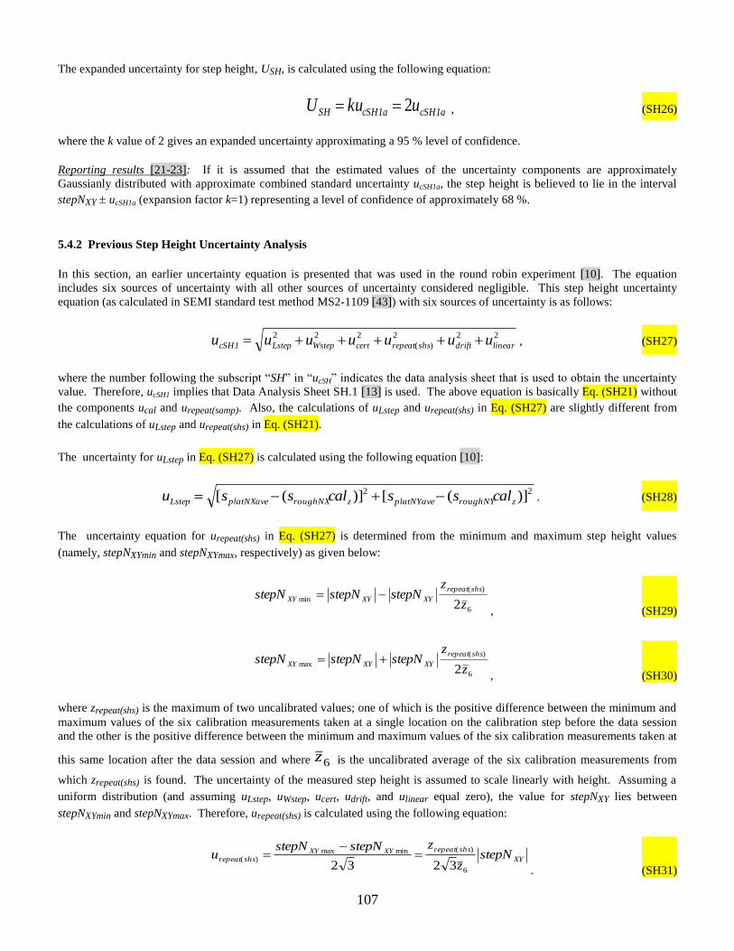
107

The expanded uncertainty for step height, USH, is calculated using the following equation:

a1cSHa1cSHSH ukuU 2 , (SH26)



Gaussianly distributed with approximate combined standard uncertainty ucSH1a, the step height is believed to lie in the interval

stepNXY ucSH1a (expansion factor k=1) representing a level of confidence of approximately 68 %.

5.4.2 Previous Step Height Uncertainty Analysis

In this section, an earlier uncertainty equation is presented that was used in the round robin experiment [10]. The equation

includes six sources of uncertainty with all other sources of uncertainty considered negligible. This step height uncertainty

equation (as calculated in SEMI standard test method MS2-1109 [43]) with six sources of uncertainty is as follows:

222

)(

222

lineardriftshsrepeatcertWstepLstep1cSH uuuuuuu , (SH27)

where the number following the subscript “SH” in “ucSH” indicates the data analysis sheet that is used to obtain the uncertainty

value. Therefore, ucSH1 implies that Data Analysis Sheet SH.1 [13] is used. The above equation is basically Eq. (SH21) without

the components ucal and urepeat(samp). Also, the calculations of uLstep and urepeat(shs) in Eq. (SH27) are slightly different from

the calculations of uLstep and urepeat(shs) in Eq. (SH21).

The uncertainty for uLstep in Eq. (SH27) is calculated using the following equation [10]:

22 )]([)]([ zroughNYplatNYavezroughNXplatNXaveLstep calsscalssu . (SH28)

The uncertainty equation for urepeat(shs) in Eq. (SH27) is determined from the minimum and maximum step height values

(namely, stepNXYmin and stepNXYmax, respectively) as given below:

6

)(

min2z

zstepNstepNstepN

shsrepeat

XYXYXY

, (SH29)

6

)(

max2z

zstepNstepNstepN

shsrepeat

XYXYXY

, (SH30)

where zrepeat(shs) is the maximum of two uncalibrated values; one of which is the positive difference between the minimum and

maximum values of the six calibration measurements taken at a single location on the calibration step before the data session

and the other is the positive difference between the minimum and maximum values of the six calibration measurements taken at

this same location after the data session and where 6z is the uncalibrated average of the six calibration measurements from

which zrepeat(shs) is found. The uncertainty of the measured step height is assumed to scale linearly with height. Assuming a

uniform distribution (and assuming uLstep, uWstep, ucert, udrift, and ulinear equal zero), the value for stepNXY lies between

stepNXYmin and stepNXYmax. Therefore, urepeat(shs) is calculated using the following equation:

XY

shsrepeatXYXYshsrepeat stepN

z

zstepNstepNu

6

)(minmax)(

3232

. (SH31)

108

Table SH4 gives example values for each of the uncertainty components in Eq. (SH27) as well as the value for the combined

standard uncertainty, ucSH1.

Table SH4. Example Step Height Uncertainty Values

From a Round Robin Bulk-Micromachined CMOS Chip


1. uLstep

variations across the length of the step 0.011 m

(using splatNXave=0.0118 m,

splatNYave=0.0102 m,

and sroughNX=sroughNY=0.0036 m)

2. uWstep

variations across the width of the step 0.0073m

(using stepNXYa=0.4928 m,

stepNXYb=0.4814 m,

and stepNXYc=0.4949 m)

3. ucert

certified value of physical step height standard

used for calibration 0.0041m

(using cert=9.887m,

cert=0.083m,

and stepNXY =0.490 m)

4. urepeat(shs)

repeatability of measurement on physical step

height standard 0.00034m

(using zrepeat(shs) =0.024 µm,

6z =9.876 µm,

and calz=1.00031)

5. udrift

drift during data session 0.00023m

(using zdrift =0.016 m

and cert=9.887 m)

6. ulinear

height linearity of data scan 0.0028m

(using zperc=1.0 % )

ucSH1 a

uncertainty of step height measurement 0.014m

= 222

)(

222

lineardriftshsrepeatcertWstepLstep uuuuuu

a This ucSH1 uncertainty (times 3) is associated with the first repeatability data point plotted in Fig. SH8 and Fig. SH9 (for TS1 in Quad 1).

5.5 Step Height Round Robin Results

The round robin repeatability and reproducibility results are given in this section for step height measurements. The

repeatability data were taken in one laboratory using a stroboscopic interferometer operated in the static mode (see Sec. 1.1.2).

A bulk-micromachined CMOS test chip with step height test structures arranged in quads, as shown in Fig. SH7 and processed

in a similar way to the MEMS 5-in-1 chip, was used in the round robin. Four step height measurements were taken from each of

the four test structures in each of three quads. Therefore, 48 step height measurements were obtained where each step height

measurement is the average of three measurements taken at the different positions (a, b, c) somewhat evenly spaced along the

width of the step as specified in Sec. 5.3.

109

Figure SH7. A design rendition of Quad 2 on the round robin test chip

For the reproducibility data, seven participants were identified and each participant was supplied with a round robin test chip.

The participant was asked to obtain the step height from any two test structures in the first of the three quads of step height test

structures. Following SEMI standard test method MS2-1109 [43] for step height measurements, the raw, uncalibrated

measurements were recorded on Data Analysis Sheet SH.1 [13].

Table SH5 presents the step height repeatability and reproducibility results. In this table, n indicates the number of calculated

step height values. The averages (namely |stepNABave|) of the repeatability and reproducibility measurement results are listed

next followed by repeat(samp), which is the relative standard deviation of the repeatability step height measurements. Then,

2stepNAB is given, which is 2.0 times the standard deviation of the repeatability or reproducibility measurements. Below this,

the average of the repeatability or reproducibility combined standard uncertainty values (ucSHave) for different calculations are

presented. (It is interesting in comparing the 2stepNAB values for |stepNAB| that the repeatability value is larger than the

reproducibility value.)

Table SH5. Step Height Measurement Results

Repeatability

results

Reproducibility

results

n 48 14

|stepNABave| 0.477 m 0.481 m

repeat(samp) 3.95 % 2stepNAB 7.9 % 6.2 %

ucSH1avea 0.014 m

(3.0 %)

0.014 m

(3.0 %)

ucSH1aaveb 0.024 m

(5.0 %)

a As determined using Eq. (SH27)

b As determined using Eq. (SH21)

Figs. SH8 and SH9 are plots of the step height round robin results. In these figures, the repeatability data are plotted first, after

which the results from the seven participants55

are plotted. At the top of these figures, |stepNABave| and 3ucSHave (as obtained or

derived from Table SH5) are specified for the repeatability data. The values for |stepNABave| ± 3ucSHave are also plotted in these

figures with both the repeatability and reproducibility data.56

Observe that all of the reproducibility results fall comfortably

between the repeatability bounds of |stepNABave| ± 3ucSHave.

55

Participant #2 provided stylus profilometer results using average roughness values instead of standard deviation values (because that instrument did not

provide standard deviation values). Therefore, in the analysis for that laboratory average roughness values were inserted into the data sheet for analysis as

opposed to standard deviation values. 56

Table SH4 specifies the value of each of the uncertainty components comprising the 3ucSH1 uncertainty bars for the first repeatability data point plotted in Fig.

SH8 and in Fig. SH9 (for TS1 in Quad 1).

110

Figure SH8. Step height round robin results with the repeatability results grouped according to quad.

57

Table SH6. Step Height Repeatability Data Grouped by Quad

Q1 Q2 Q3

n 16 16 16

|stepNABave| 0.479 m 0.473 m 0.478 m

repeat(samp) 4.2 % 3.6 % 4.2 %

±2σ limits for |stepNAB| 8.4 % 7.2 % 8.3 %

ucSH1avea 0.015 m

(3.1 %)

0.015 m

(3.2 %)

0.013 m

(2.8 %)

ucSH1aaveb 0.025 m

(5.2 %)

0.023 m

(4.8 %)

0.024 m

(5.0 %) a As determined using Eq. (SH27)


Figure SH8 groups the repeatability results by quad number. The results from Quad 1 are plotted first, followed by the results

from Quad 2, then the results from Quad 3. Within the results of each quad, the results are grouped according to test structure

number58

with the results from Test Structure 1 plotted first, followed by the results from Test Structure 2, etc. For each quad,

the average step height value and the ±2σ limits for this value are given at the bottom of Fig. SH8 and also in Table SH6. The

results among the quads are comparable implying there are no discernible variations in the step height value between

neighboring quads.

57

Republished with permission from Semiconductor Equipment and Materials International, Inc. (SEMI) © 2011. 58

The upper left hand step height test structure in a quad, such as shown in Fig. SH7, is called Test Structure 1 and it has a 0 orientation. Test Structure 2 (the

upper right test structure) has a 270 orientation, Test Structure 3 (the bottom right test structure) has a 180 orientation, and Test Structure 4 (the bottom left

test structure) has a 90 orientation.

111

Figure SH9. Step height round robin results with the repeatability results grouped according to test structure number

59

Table SH7. Step Height Repeatability Data Grouped by Test Structure

TS1 TS2 TS3 TS4

n 12 12 12 12

|stepNABave| 0.486 m 0.469 m 0.474 m 0.478 m

repeat(samp) 3.2 % 4.4 % 3.5 % 4.3 %

±2σ limits for |stepNAB| 6.4 % 8.7 % 7.0 % 8.5 %

ucSH1avea 0.014 m

(2.8 %)

0.015 m

(3.1 %)

0.011 m

(2.4 %)

0.018 m

(3.7 %)

ucSH1aaveb 0.021 m

(4.3 %)

0.025 m

(5.4 %)

0.020 m

(4.2 %)

0.027 m

(5.6 %) a As determined using Eq. (SH27)


Figure SH9 groups the repeatability results by test structure number. The results from Test Structure 1 (TS1) are plotted first,

followed by the results from Test Structure 2 (TS2), followed by the results from Test Structure 3 (TS3), then Test Structure 4

(TS4). Within the results for each test structure, the results are grouped according to quad with the results from Quad 1 plotted

first, followed by the results from Quad 2, then the results from Quad 3. As in Fig. SH8, for each test structure the average step

height value and the ±2σ limits for this value are given at the bottom of Fig. SH9 and also in Table SH7. It is interesting that

TS1 and TS3 (which are rotated 90 with respect to TS2 and TS4) have comparable ±2σ limits as do TS2 and TS4; however

the ±2σ limits for TS1 and TS3 are slightly less than the ±2σ limits for TS2 and TS4 when they should be comparable. In

addition, there are more variations in the average step height value between rotated test structures (as shown in Fig. SH9 and

Table SH7) than variations between quads (as shown in Fig. SH8 and Table SH6).

59

Republished with permission from Semiconductor Equipment and Materials International, Inc. (SEMI) © 2011.

112

The platform surfaces involved in the measured steps are not ideal surfaces. Often they are tilted (even though the data are

leveled with respect to the reference platform) and the data jagged. The standard deviations obtained from these surfaces is

affected by the selection of the analysis regions (including the number of data points within these regions). A more

comprehensive determination of the length and width variations may be necessary when dealing with tilt. Repeatability might

also be improved by calculating the step height from fitted straight lines as described for NIST step height calibrations [45] and

outlined in ASTM E 2530 [46]. As stated in [45], “For step height measurements, one of several algorithms may be used. For

single-sided steps, a straight line is fitted by the method of least squares to each side of the step transition, and the height is

calculated from the relative position of these two lines extrapolated to the step edge.”

Calibration of the interferometer or comparable instrument in the out-of-plane z-direction is considered mandatory for step

height measurements. Without this calibration, a bias to the measurements is expected with the direction and degree of the bias

being different for each magnification.

5.6 Using the MEMS 5-in-1 to Verify Step Height Measurements

To compare your in-house step height measurements with NIST measurements, you will need to fill out Data Analysis Sheet

SH.1.a. (This data analysis sheet is accessible via the URL specified in the reference [13], a reproduction of which is given in


calculations, the data on your completed form can be compared with the data on the RM Report of Investigation and the


Calibrate the instrument: Calibrate the instrument as given in Sec. 5.2. Obtain the inputs for Table 1 in Data Analysis Sheet

SH.1.a.

Locate the step height test structure: In the fourth grouping of test structures on the MEMS 5-in-1 chips shown in Fig. 1 and

Figs. 2(a and b) for RM 8096 and RM 8097 (fabricated on MUMPs98 and MUMPs95), step height measurements are made.

Step height test structures are provided for the purpose, such as shown in Fig. SH1(a) for RM 8096 and as shown in Fig. SH1(b)

for RM 8097. Specifications for the step height test structures on the chips shown in Fig. 1 and Figs. 2(a and b) are given in

Table SH1 and Table SH2, respectively.

Data Analysis Sheet SH.1.a requires measurements from one step height test structure on the MEMS 5-in-1 chip. The step

height test structure to be measured can be deduced from the data entered on the NIST version of the Data Analysis Sheet

SH.1.a, which accompanies the RM.

For the step height grouping of test structures for RM 8096, as shown in Fig. SH1(a), the target test structure can be found as

follows:

1. The input which (i.e., input #4 on Data Analysis Sheet SH.1.a) specifies which of the six step height measurements to

take in the fourth grouping of test structures. Using the arrows as a guide in Fig. SH1(a), the first measurement is taken

from the first step height test structure, the second and third measurements are taken from the second step height test

structure, the fourth measurement is taken from the third step height test structure, and the fifth and sixth measurements

are taken from the fourth step height test structure. (Measurements from the fourth step height test structure should be

taken with a stylus instrument or instrument not affected by the reflectivity of the sample surface, unless the chip is

covered with a smooth reflective material before measurement.)

2. The input which2 (i.e., input #5) specifies which iteration of the test structure in the set of three possible target test

structures of the same design where “first” corresponds to the topmost test structure in the column.

For the step height grouping of test structures for RM 8097, as shown in Fig. SH1(b), the target test structure can be found as

follows:

1. The input which (i.e., input #4) indicates which of the five quads depicted in Fig. SH1(b) contains the target step height

test structure.

2. The input orient (i.e., input #6) is used to locate the target test structure within the selected quad. There are four step

height test structures in each quad with each test structure having a different orientation (0, 90, 180, or 270). The

upper left hand step height test structure has a 0 orientation, the bottom left test structure has a 90 orientation, the

bottom right test structure has a 180 orientation, and the upper right test structure has a 270 orientation.

Take the measurements: Following the steps in SEMI standard test method MS2 [4] for measuring step heights, the step height

measurements are obtained using the highest magnification objective that is available and feasible (e.g., a 20 objective). The

data are leveled and zeroed with respect to the top of the surrounding or partially surrounding reference platform. Three 2D data

traces (Trace a, Trace b, and Trace c, as shown in Fig. SH2 and Fig. SH3) are used to obtain the step height measurement. For

113

the step height test structure in Fig. SH2, given the step of interest pointed to by the arrow in this figure, the platform height

measurements for Platforms A and B and standard deviations along Traces a, b, and c are recorded. For the test structure shown

in Fig. SH3, the measurements and standard deviations are obtained from both central platforms. Therefore, twelve

measurements are obtained, six from the first platform and six from the second platform. For example, the four quantities

calculated from Trace a are platNXa, platNYa, splatNXa, and splatNYa. Analogous quantities are calculated from Traces b and c.

Perform the calculations: Enter the data into Data Analysis Sheet SH.1.a as follows:

1. Press the “Reset this form” button. (One of these buttons is located near the top of the data analysis sheet and the

other is located near the middle of the data analysis sheet.)

2. Supply the inputs to Table 1 and Table 2.

3. Press the “Calculate and Verify” button to obtain the results for the step height test structure. (One of these

buttons is located near the top of the data analysis sheet and the other is located near the middle of the data

analysis sheet.)




5. Print out the completed data analysis sheet to compare both the inputs and outputs with those on the NIST-

supplied data analysis sheet.

Compare the measurements: The Report of Investigation accompanying the MEMS 5-in-1 specifies a step height value (for

example, step1AB) and the expanded uncertainty, USH, (with k=2) intended to approximate a 95 % level of confidence. It is your

responsibility to determine an appropriate criterion for acceptance, such as given below:

22

)()( SHcustomerSHABcustomerABSH UU1step1stepD , (SH32)

where DSH is the absolute value of the difference between your step height value, e.g., step1AB(customer), and the step height

value on the RM Report of Investigation, step1AB, and where USH(customer) is your expanded uncertainty value and USH is the

expanded uncertainty on the RM Report of Investigation. If your measured value for step height (as obtained in the newly filled

out Data Analysis Sheet SH.1.a) satisfies your criterion for acceptance and there are no pertinent “wait” statements at the bottom

of your Data Analysis Sheet SH.1.a, you can consider yourself to be appropriately measuring step height according to the SEMI

MS2 step height standard test method [4] according to your criterion for acceptance.



114

6 Grouping 5: In-Plane Length

An in-plane length (or deflection) measurement is defined as the experimental determination of the straight-line distance

between two transitional edges in a MEMS device. A transitional edge is an edge of a MEMS structure that is characterized by

an abrupt change in surface slope. Many times, more precise in-plane length values can be obtained by using the design

dimensions as opposed to using measurements taken with an optical interferometric microscope (which typically provides more

precise measurements than an optical microscope [14]). Therefore, ASTM standard test method E 2244 [5] on in-plane length

measurements is used when measuring in-plane deflections and when measuring lengths in fabrication processes that are being

developed.

This section on in-plane length is not meant to replace but to supplement the ASTM standard test method E 2244 [5], which

more completely presents the scope, significance, terminology, apparatus, and test structure design as well as the calibration

procedure, measurement procedure, calculations, precision and bias data, etc. In this section, the NIST-developed in-plane

length test structures on RM 8096 and RM 8097, as shown in Fig. 1 and Figs. 2(a and b) in the Introduction are given in Sec.

6.1. Sec. 6.2 discusses the calibration procedure for the in-plane length measurements, and Sec. 6.3 discusses the in-plane

length measurement procedure. Following this, the uncertainty analysis is presented in Sec. 6.4, the round robin results are

presented in Sec. 6.5, and Sec. 6.6 describes how to use the MEMS 5-in-1 to verify in-plane length measurements.

6.1 In-Plane Length Test Structures

In-plane length measurements are taken in the fifth grouping of test structures, as shown in Fig. L1(a) for RM 8096 depicted in

Fig. 1 and as shown in Fig. L1(b) for RM 8097 depicted in Figs. 2(a and b).

(a)

(b)

Figure L1. The in-plane length grouping of test structures (a) on RM 8096, fabricated on a multi-user 1.5 m CMOS process

[8] followed by a bulk-micromachining etch, as depicted in Fig. 1 and (b) on RM 8097, fabricated using a polysilicon multi-

user surface-micromachining MEMS process [9] with a backside etch, as depicted in Figs. 2(a and b).

x

y

x

y

115

An in-plane length test structure from the grouping shown in Figs. L1(a and b) is given in Fig. L2(a) and Fig. L3(a),

respectively, with an applicable data trace taken from these test structures given in Fig. L2(b) and Fig. L3(b), respectively.

(a)

(b)

Figure L2. For an in-plane length test structure on RM 8096, (a) a design rendition and (b) an example of a 2D data trace used to determine L, as shown in (a).

(a)

Edge 4 Edge 3

y

x L a΄

Edge 3 Edge 4

m2 a e e΄

a΄

e

L


p

g

q

h

poly0

poly1


y

x

e΄

a

116

(b)

-0.5

0

0.5

1

1.5

2

2.5

3

3.5

4

4.5

0 0.2 0.4 0.6 0.8 1 1.2

z(µ

m)

x (mm)

Data along Trace a΄, a, e or e΄

Edge 1Edge 2

Edge 5

p

q

Figure L3. For a poly1 in-plane length test structure on RM 8097, (a) a design rendition and

(b) an example of a 2D data trace used to determine L, as shown in (a).

The in-plane length measurements are made with an interferometric microscope. Many interferometric microscopes are

purchased with five magnifications (5, 10, 20, 40, and 80). Therefore, for each of these magnifications, an in-plane

length test structure is provided in both of the in-plane length groupings of test structures in Figs. L1(a and b). The design

length, Ldes, for the test structure designed for the specified magnification is given in Table L1. This table also includes a

maximum field of view for each magnification for a representative c-mount camera.60

In most cases, Ldes is at least 70 m less

than this value.

Table L1. Design Lengths on RM 8096 and RM 8097 for the Given Magnifications

Magnification

Calibrated Maximum

Field of View

(in the x-direction)

Ldes

5 1165.00 m 1000 m

10 599.998 m 500 m

20 287.00 m 200 m

40 150.000 m 80 m

80 75.0000 m 24 m

For RM 8096: As can be seen in Fig. L1(a), the design length, Ldes, for the in-plane length test structures is specified at the top

of each column of test structures. This is the design length specified in Table L1. The design width is 28 m. There are three

occurrences of each in-plane length test structure, one of which is shown in Fig. L2(a) and Fig. L4. For each test structure, the

following three types of in-plane length measurement can be obtained for the given design length:

1. An outside edge-to-outside edge length measurement, as given by Loo in Fig. L4, where Edge 1 and Edge 2 are

considered outside edges,

2. An inside edge-to-inside edge length measurement, as given by Lii in Fig. L4, where Edge 3 and Edge 4 are

considered inside edges, and

3. An inside edge-to-outside edge length measurement, as given by Lio in Fig. L4, where Edge 5 is considered an

inside edge and Edge 6 is considered an outside edge. (We will consider this measurement comparable to an

outside edge-to-inside edge length measurement, Loi.)

60

For this interferometric microscope, the resolution in the x-direction is better than the resolution in the y-direction.

117

Figure L4. A design rendition of an in-plane length test structure on RM 8096.

The design layer for the test structure given in Fig. L4 is metal2 (or m2), which is the topmost metal layer in the process. This

m2 layer is encompassed in oxide. The 2D data trace given in Fig. L2(b) shows the existence of two transitional edges assumed

to be Edge 3 and Edge 4 in Fig. L2(a). In fact, these edges may be due to the oxide layer as it traverses over the metal2. This

would cause an offset, Loffset, to the measured m2-to-m2 in-plane length value, L, given in Fig. L2(a) as discussed in Sec. 6.3.

For RM 8097: As seen in Fig. L1(b), the in-plane length grouping of test structures on RM 8097 includes both fixed-fixed

beams and cantilevers [comprised of either poly1 (or p1) or poly2 (or p2)] as in-plane length test structures. For the

measurements supplied on the RM 8097 Report of Investigation, we will only be concerned with the fixed-fixed beam arrays.

There are two p1 fixed-fixed beam arrays and one p2 fixed-fixed beam array. The two p1 arrays of fixed-fixed beams are

located on the left hand side of the in-plane length grouping of test structures in Fig. L1(b) and the one p2 array is the middle

array in the bottom row. The beams in the bottom p1 array and the p2 array have a 0 orientation and the beams in the top p1

array have a 90 orientation. The fixed-fixed beams in these three arrays are designed with the lengths, Ldes, specified in Table

L1, with three occurrences of each beam. This design length is specified (in micrometers) next to the second occurrence of each

test structure. The design width of all these beams is 20 m. An example poly1 fixed-fixed beam test structure is shown in Fig.

L3(a). The in-plane length measurement, L, is taken between the edges of the anchor lips of the fixed-fixed beam [i.e., between

Edges 1 and 2 in Fig. L3(a)]. An example 2D data trace is given in Fig. L3(b).

6.2 Calibration Procedure for In-Plane Length Measurements

For RM in-plane length measurements, the interferometric microscope is calibrated in the z-direction to obtain the z-calibration

factor, calz, as specified in Sec. 5.2 for step height calibrations. The interferometric microscope is also calibrated in the x- and

y-directions as given below. These calibration procedures are the same as those for residual strain and strain gradient

measurements, as indicated in Sec. 3.2 and Sec. 4.2, respectively.

To calibrate the interferometric microscope in the x- and y-directions [2-3,5], a 10 m grid (or finer grid) ruler is used with each

combination of lenses. The following calibration is performed on a yearly basis, or after the instrument has been serviced:

1. The ruler is oriented in the x-direction and rulerx is recorded as the maximum field of view in the x-direction for

the given combination of lenses (as measured on the screen of the interferometric microscope). The value for xcal

is estimated, wherexcal is the standard deviation in a ruler measurement in the interferometric microscope’s x-

direction for the given combination of lenses.

2. The x-calibration factor, calx, is calculated using the following equation:

x

x

xscope

rulercal , (L1)

where scopex is the interferometric microscope’s maximum field of view in the x-direction for the given

combination of lenses (or typically, the maximum x-value obtained from an extracted 2D data trace).

3. The above two steps are repeated in the y-direction to obtain caly.

Loo

Lii

Lio

y

x

Edge 1 Edge 2

Edge 3 Edge 4

Edge 5

Edge 6 m2

118

4. The x- and y-data values obtained during the data session are multiplied by the appropriate calibration factor to

obtain calibrated x- and y-data values.

6.3 In-Plane Length Measurement Procedure

In-plane length measurements are taken between two transitional edges, such as Edges 1 and 2 in Fig. L3(a). A transitional edge

is an edge of a MEMS structure that is characterized by an abrupt change in surface slope, as seen in Fig. L3(b) for say, Edges 1

and 2. From each of four 2D data traces, an x-value is obtained at each transitional edge defining the in-plane length

measurement. The two outermost data traces [e.g., Traces a΄ and e΄ in Fig. L3(a)] are typically used for alignment purposes.

From these outermost data traces, the y-values are also obtained. The in-plane length is calculated using the acquired x- and y-

values.

To obtain an in-plane length measurement, consult the standard test method [5]. Briefly, the following steps are taken for RM

8097, and a slightly modified procedure [5] is followed for RM 8096:

1. If the transitional edges that define the in-plane length measurement face each other [such as Edge 1 and Edge 2 in

Fig. L3(a)], Traces a΄, a, e, and e΄, also shown in Fig. L3(a), are extracted from a 3-D data set. The uncalibrated

values from Edge 1 and Edge 2 (namely, for x1uppert and x2uppert to be described in the next step) are obtained

from each 2D data trace [one of which is shown in Fig. L3(b)]. The trailing subscript “t” indicates the data trace

(a΄, a, e, or e΄) being examined. The y values associated with Traces a΄ and e΄ are also recorded.

2. To find xupper: The upper transitional x-data value, xupper, is found as follows. The x values are examined between

Point p and Point q in Figs. L3(a and b). The x-value that most appropriately locates the upper corner of the

transitional edge is called xupper, or x1upper in this case since it is associated with Edge 1. At times it is easy to

identify one point that accurately locates the upper corner of the transitional edge. In this case, the maximum

uncertainty associated with the identification of this point is ±nt xres calx, where nt = 1 and xres is the uncalibrated

resolution of the interferometric microscope in the x-direction. This value of n1t = 1 is also recorded. For a less

obvious point that locates the upper corner of the transitional edge, the value for n1t would be larger than one. If

n1t is larger than four, it is recommended that another 2D data trace be obtained or another 3-D data set.

3. If an in-plane length measurement is determined between transitional edges that face each other, such as Edge 1

and Edge 2 in Figs. L3(a and b), then the measured in-plane length for each 2D data trace, Lmeast, is calculated

using the following equation:

xuppertuppertmeast cal1x2xL )( , (L2)

where a trailing subscript “t” indicates the data trace (a΄, a, e, or e΄) being examined. The measured length, Lmeas,

is calculated as follows:

4

emeasmeasemeasaameasmeas

LLLLL

. (L3)

To account for misalignment, the aligned length, Lalign, is calculated using the following equation:

cosmeasalign LL , (L4)

where the misalignment angle, α, is shown in Fig. L5(a). This misalignment angle is typically determined using

the two outermost data traces [a΄ and e΄ in this case, as seen in Fig. L3(a)] and is calculated to be either α1 or α2

using either Δx1 or Δx2, respectively [as seen in Fig. L5(b)]. The equations for Δx1 and Δx2 are:

eupperaupper 1x1x1x , and (L5)

eupperaupper 2x2x2x . (L6)

119

The equation for α is as follows:

y

x

cal

cal

y

x1tan , where (L7)

ea yyy , (L8)

and where ya΄ and ye΄ are the uncalibrated y-values associated with Traces a΄ and e΄, respectively. In addition,

if ,eaea 2n2n1n1n then1 and ,1xx (L9)

and if

,eaea 2n2n1n1n then2 and 2.xx (L10)

The effect of the misalignment angle, α, is expected to be much smaller (almost negligible) for the shorter length

measurements (< 200 µm at a magnification of 20×) because for these measurements it is easier to visually align

the sample within the field of view of the interferometric microscope before taking a 3-D data set than it is for the

longer length measurements (> 500 µm at a magnification of 10×).

(a) (b)

Figure L5. Drawings depicting (a) the misalignment angle, α, and (b) the misalignment between the 2D

data traces a΄ and e΄ and Edges 1 and 2. In drawing (b) it is assumed the x- and y-values are calibrated.

The equation for the in-plane length, L, is a follows:

offsetalign LLL , (L11)

where Loffset is the in-plane length correction term for the given type of in-plane length measurement [for example,

for an inside edge-to-inside edge length measurement, Lii as seen in Fig. (L4)] on similar structures, when using

similar calculations, and for a given magnification of a given interferometric microscope. As specified in Sec. 6.1

for RM 8096, Edges 3 and 4 in Fig. L2(b) may be due to the oxide covering the m2 layer in Fig. L2(a), in which

case Loffset is used as a correction term to provide a measurement between the two m2 lines in Fig. L2(a). In

addition, the interferometric software may treat data at transitional edges differently (for example, if neighboring

data points are averaged together) which could add to the offset of an in-plane length measurement. The

determination of Loffset is discussed in the next step.

4. To determine Loffset (mentioned above) for a given magnification of a given interferometric microscope for a given

type of in-plane length measurement on similar structures when using similar calculations, at least twelve 3-D data

Trace a΄

Trace e΄

(x1uppera΄, ya΄) (x2uppera΄, ya΄)

(x1uppere΄, ye΄) (x2uppere΄, ye΄)

Edge 2 Edge 1 Δy

Δx2

Δx1

α1

α2

Lmeasa΄

Lmease΄

α Lmeas

Lalign

120

sets are obtained and Lalign is calculated as given above. The average of these twelve or more measurements,

Lalignave, is subtracted from Ldes to find Loffset, where Ldes is the design length. An alternate measurement of Loffset

is determined from four measurements of Lalign for both Lii and Loo in Fig. L4 using four 3-D data sets. The

average of these values (namely, Liialignave and Looalignave, respectively) is determined. Then Loffset is calculated as

(Looalignave–Liialignave)/2.

5. If the transitional edges that define the in-plane length measurement are oriented in the same direction and have

similar slopes and magnitudes [such as Edge 1 and Edge 5 in Figs. L3(a and b)], Traces a΄, a, e, and e΄ are

extracted from a 3-D data set as specified in step 1. However, for each data trace, a measured x-value is obtained

at the upper portion of each transitional edge (xupper) as specified in step 2 or a measured x-value is obtained at the

lower portion of each transitional edge (xlower) as also specified in step 2 but replacing “upper” with “lower.” The

upper values are used unless the lower values are easier to locate. (In other words, the upper values are used

unless n1t + n5t for the lower values are typically smaller than those for the upper values.) To find the in-plane

length, the equations are similar to those used above when the in-plane length measurement is taken between

transitional edges that face each other; however, when and if appropriate the lower values replace the upper values

and the pertinent edges are referenced. Due to the similarities of the edges involved when the transitional edges

that define the in-plane length measurement face the same direction, a length correction term, Loffset, is not needed

and the in-plane length, L, is equated with Lalign, as given in Eq. (L4).

6.4 In-Plane Length Uncertainty Analysis

In this section, three uncertainty equations are presented for use with in-plane length. The first one (presented in Sec. 6.4.1) is

used for the MEMS 5-in-1. The other two (presented in Sec. 6.4.2) were used in the round robin experiment and other previous

work.

6.4.1 In-Plane Length Uncertainty Analysis for the MEMS 5-in-1

This section presents the six-term combined standard uncertainty equation [5] used with the MEMS 5-in-1. The six sources of

uncertainty are a) the uncertainty of the in-plane length measurement (uL), b) the uncertainty due to four measurements taken

on the test structure at different locations (urepeat(L)), c) the uncertainty of the calibration of the interferometric microscope in

the x-direction (uxcal), d) the alignment uncertainty (ualign), e) the uncertainty of the value for Loffset (uoffset), and f) the

uncertainty due to the repeatability of similar measurements taken on test structures processed similarly to the one being

measured (urepeat(samp)). The combined standard uncertainty equation [5] can be written as follows:

2

)(

2222

)(

2

0 samprepeatoffsetalignxcalLrepeatLcL uuuuuuu , (L12)

where a number (or a number and a letter) following the subscript “L”in “ucL” indicates the data analysis sheet that is used to

obtain the combined standard uncertainty value. Therefore, ucL0 implies that Data Analysis Sheet L.0 [5,13] is used. In

determining the combined standard uncertainty, a statistical Type A analysis is used to obtain urepeat(L) and urepeat(samp). The

other sources of uncertainty are obtained using a Type B evaluation [21-23] (i.e., one that uses means other than the statistical

Type A analysis).

Table L2 provides the equations for the uncertainty components. The first uncertainty component in Eq. (L12) and listed in

Table L2 is uL. The value for uL is determined from the minimum and maximum length values (namely, LminL and LmaxL) as

calculated using the equations given in Table L2. Assuming a 99.7 % nominal probability of coverage, the range of values for L

due to this component is LmaxL – LminL. Further, if a Gaussian probability distribution is assumed, uL is calculated using the

formula given in the last column of Table L2, which is repeated below:

6

minLmaxLL

LLu

. (L13)

121

It is assumed that the uncertainty associated with the pixel resolution in the x-direction is incorporated within this uncertainty

component.

The second uncertainty component in Eq. (L12) and listed in Table L2 is urepeat(L). This uncertainty component is determined

from σrepeat(L), the calibrated one sigma standard deviation of the in-plane length measurements Lmeasa΄, Lmeasa, Lmease, and

Lmease΄. The equation used to calculate urepeat(L) is given in the last column of Table L2. This is a statistical Type A component.

Table L2. In-Plane Length Uncertainty Equations for the MEMS 5-in-1 [5]

Lmin Lmax G or

Ua

/ A or

Bb

equation

1. uL cosmeasminminL LL

offsetL

where

ameasminmeasmin LL (

measminemeasmina LL

4/)emeasminL

meastmeasmint LL

xrestt calx2n1n )(

cosmeasmaxmaxL LL

offsetL

where

ameasmaxmeasmax LL (

measmaxemeasmaxa LL

4/)emeasmaxL

meastmeasmaxt LL

xrestt calx2n1n )(

G / B

6

minLmaxLL

LLu

2. urepeat(L) – – G / A cos)()( LrepeatLrepeatu

cos),

,,(

emeasmease

measaameas

LL

LLSTDEV

3. uxcal – – G / B

cosmeas

x

xcal

xcal Lruler

u

4. ualign minmeasminalign LL cos

offsetL

using Eq. (L14) for αmin

maxmeasmaxalign LL cos

offsetL

using Eq. (L15) for αmax

U / B

32

minalignmaxalign

align

LLu

5. uoffset –

–

G / B

3

offset

offset

Lu

6. urepeat(samp) – G / A )()( samprepeatsamprepeatu



The third uncertainty component in Eq. (L12) and listed in Table L2 is uxcal. This uncertainty component is determined from

the estimated value of σxcal obtained in Sec. 6.2 and is assumed to scale linearly with the aligned length (i.e., Lmeascosα) as

given in Table L2. This uncertainty component assumes that the uncertainty of the calibration is due solely to the uncertainty of

the calibration in the x-direction (in other words, the effect of σycal on the misalignment angle, α, is considered negligible).

Similarly, it is assumed that the effect of σxcal on the misalignment angle, α, is considered negligible.

122

The fourth uncertainty component in Eq. (L12) and listed in Table L2 is ualign. This uncertainty component is determined from

the minimum and maximum length values (namely, Lminalign and Lmaxalign) given in this table resulting from calculated

minimum and maximum values for the misalignment angle, α. These equations for αmin and αmax are given below:

y

xres

y

x

mincal

cal

y

x

cal

cal

y

x 2tan 1 , (L14)

y

xres

y

x

maxcal

cal

y

x

cal

cal

y

x 2tan 1 , (L15)

where Δy is given in Eq. (L8) and Δx is equated with either Δx1 or Δx2 in Eq. (L5) or Eq. (L6), respectively, as determined in

Eq. (L9) or Eq. (L10). A uniform probability distribution is assumed in the calculation of ualign.

The fifth uncertainty component in Eq. (L12) and listed in Table L2 is uoffset, which is assumed to be equivalent to |Loffset|, as

determined in Sec. 6.3, divided by three. Besides the uncertainty of the value of Loffset, uoffset is also assumed to incorporate

geometrical uncertainties along the applicable edges. For in-plane length measurements when the transitional edges face the

same direction, it is assumed that Loffset = uoffset=0.

The sixth uncertainty component in Eq. (L12) and listed in Table L2 is urepeat(samp), which is equated with repeat(samp)΄, the

repeatability standard deviation for in-plane length test structures. This value of repeat(samp)΄ is found from at least twelve 3-D

data sets taken on similar test structures from which twelve values of Lalign are calculated as given in Sec. 6.3. The standard

deviation of the twelve or more measurements of Lalign is equated with repeat(samp)΄. Table 3 in Sec. 1.14 specifies the value for

repeat(samp)΄ for test structures with edges that face each other, with an approximate design length of 200 m, and fabricated by

a bulk micromachining process similar to that used to fabricate RM 8096 when using a magnification of 25 for a measurement

between two metal2 lines. For RM 8097, the value for repeat(samp)΄ is given in Table 4.

The expanded uncertainty for in-plane length, UL, is calculated using the following equation:

0cL0cLL ukuU 2 , (L16)



Gaussianly distributed with approximate combined standard uncertainty ucL0, the in-plane length is believed to lie in the interval

L ucL0 (expansion factor k=1) representing a level of confidence of approximately 68 %.

6.4.2 Previous In-Plane Length Uncertainty Analyses

Two previous versions of the combined standard uncertainty equation exist. For these versions, the in-plane length, L, is

calculated using the following equation:

2

maxLminLmeas

LLLL

, (L17)

where LminL and LmaxL are specified in a following paragraph. In addition, alignment is ensured (such that α = 0) and L is

determined from one data trace.

123

The first combined standard uncertainty equation is used with the round robin results that are presented in the next section. The

following three term uncertainty equation is used [47]:

222

xresxcalL1cL uuuu . (L18)

The first uncertainty component in the above equation is uL, which is determined from the minimum and maximum length

values (namely, LminL and LmaxL) as calculated from one data trace using the following equations for transitional edges that face

each other:61

xlowerlowerminL cal1x2xL , and (L19)

xupperuppermaxL cal1x2xL . (L20)

Assuming a 99.7 % nominal probability of coverage, the range of values for L due to this component is LmaxL–LminL. Further, if

a Gaussian probability distribution is assumed, uL is calculated using Eq. (L13). For transitional edges that are oriented in the

same direction, the following equations are used:

xresminL calxLL 2 , and (L21)

xresmaxL calxLL 2 , (L22)

such that uL in Eq. (L13) can be simplified to be:

3

2 xresL

calxu . (L23)

This is a Type B component.

The second uncertainty component in Eq. (L18) is uxcal, which is calculated using the equation given in Table L2 with α = 0 and

Lmeas determined using Eqs. (L17), (L19), and (L20) or Eqs. (L17), (L21), and (L22), as appropriate.

The third uncertainty component in Eq. (L18) is uxres. For this uncertainty component, Lminres and Lmaxres are determined from

one 2D data trace using the following equations:

xresmeasminres calxLL , (L24)

xresmeasmaxres calxLL , (L25)

where xres is the uncalibrated pixel resolution of the interferometric microscope in the x-direction. Assuming a uniform

distribution for this uncertainty component of width 2xres, uxres is calculated using the equation given below:

332

xresminresmaxres

xres

calxLLu

, (L26)

61

Consult ASTM E 2244–05 [47] for slight differences from the MEMS 5-in-1 approach concerning the determination of the upper and lower

x-values used to obtain LminL and LmaxL.

124

where uxres is a Type B component.

Eq. (L18) is used in Data Analysis Sheet L.1 [13] with Table L3 giving example values for each of these uncertainty

components as well as the combined standard uncertainty value, ucL1. The original uncertainty equation [48] consists of only the

first term in Eq. (L18).

Table L3. Example In-Plane Length Uncertainty Values

From a Round Robin Surface-Micromachined Chip Using Eq. (L18)


1. uL

in-plane length measurement 0.911ma

(using x1upper = 18.872 m,

x1lower = 21.9532 m,

x2lower = 215.68 m,

x2upper = 217.991 m,

and calx =1.01385)

2. uxcal

calibration in x-direction 0.463 m

(using xcal = 0.667m,

rulerx /calx = interx = 283.08m,b

and L =199.14 m)

3. uxres

interferometric resolution in the x-direction 0.225m

(using xres = 0.3851 m)

ucL1

combined standard uncertainty for in-plane length 1.05mc

222

xresxcalL uuu

a This uL uncertainty value is one of the 48 repeatability values which comprise the average value, uLave, as given in

Table L4 and plotted in Fig. L9 for Ldes=200 m.

b Interx is also called scopex.

c For transitional edges that face each other, such as Edges 1 and 2 in Figs. L3(a and b) at a magnification of 20 [11,47]

6.5 In-Plane Length Round Robin Results

The round robin repeatability and reproducibility results are given in this section for in-plane length measurements. The

repeatability data were taken in one laboratory using an optical interferometric microscope (see Sec. 1.1.2). Unlike the MEMS

5-in-1 chips shown in Figs. 2(a and b), a similarly processed surface-micromachined test chip (from MUMPs46 [9] and without

the backside etch) was fabricated on which in-plane length measurements were taken from each of the fixed-fixed beams

depicted in Fig. L6. The design length (in micrometers) of each of these beams is specified to the left of these test structures.

This design length corresponds to the design length of LA in Fig. L7. The measurement of LA [or L in Fig. L3(a)] is obtained

from the data along Edges 1 and 2 using Trace a or Trace e. Example 2D data from Trace a or Trace e are given in Fig. L3(b).

Trace a or Trace e can also be used to obtain the in-plane length measurement, LB, as shown in Fig. L7 from data along Edges 1

and 5. The design lengths for the measurements of LB on the test structures shown in Fig. L6 are 1035m, 535m, 235m,

115m, and 60 m (35 m more than the corresonding design values for LA). For the repeatability data, 24 measurements of

LA and 24 measurements of LB were taken on each of the five test structures in Fig. L6 and the same number of measurements

were taken on a similiarly designed array of test structures with a 90 orientation with respect to the orientation shown in Fig.

L6.

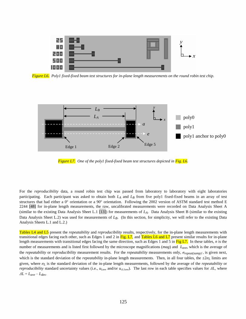
125

Figure L6. Poly1 fixed-fixed beam test structures for in-plane length measurements on the round robin test chip.

Figure L7. One of the poly1 fixed-fixed beam test structures depicted in Fig. L6.

For the reproducibility data, a round robin test chip was passed from laboratory to laboratory with eight laboratories

participating. Each participant was asked to obtain both LA and LB from five poly1 fixed-fixed beams in an array of test

structures that had either a 0 orientation or a 90 orientation. Following the 2002 version of ASTM standard test method E

2244 [48] for in-plane length measurements, the raw, uncalibrated measurements were recorded on Data Analysis Sheet A

(similar to the existing Data Analysis Sheet L.1 [13]) for measurements of LA. Data Analysis Sheet B (similar to the existing

Data Analysis Sheet L.2) was used for measurements of LB. (In this section, for simplicity, we will refer to the existing Data

Analysis Sheets L.1 and L.2.)

Tables L4 and L5 present the repeatability and reproducibility results, respectively, for the in-plane length measurements with

transitional edges facing each other, such as Edges 1 and 2 in Fig. L7, and Tables L6 and L7 present similar results for in-plane

length measurements with transitional edges facing the same direction, such as Edges 1 and 5 in Fig L7. In these tables, n is the

number of measurements and is listed first followed by the microscope magnifications (mag) and Lave, which is the average of

the repeatability or reproducibility measurement results. For the repeatability measurements only, σrepeat(samp)΄, is given next,

which is the standard deviation of the repeatability in-plane length measurements. Then, in all four tables, the ±2σL limits are

given, where σL is the standard deviation of the in-plane length measurements, followed by the average of the repeatability or

reproducibility standard uncertainty values (i.e., uLave and/or ucL1ave). The last row in each table specifies values for ΔL, where

ΔL = Lave – Ldes.

LA

Edge 1 Edge 2

x

y

Edge 5

LB

a

e

poly0

poly1


126

Table L4. Repeatability and Uncertainties of NIST Measurement Results for In-Plane Length

Measurements When the Transitional Edges Face Each Other

Design Length (Ldes) 25 m 80 m 200 m 500 m 1000 m

n 48 48 48 48 48

mag 80× 40× 20× 10× 5×

Lave 24.37 m 79.76 m 199.10 m 495.0 m 995.5 m

repeat(samp)΄ 0.10 µm 0.086 µm 0.15 µm 0.80 µm 2.5 µm

±2σL limits ±0.20 m

(±0.81 %)

±0.17 m

(±0.22 %)

±0.30 m

(±0.15 %)

±1.6 m

(±0.32 %)

±5.0 m

(±0.50 %)

uLavea

0.23 m

(0.95 %)

1.0 m

(1.3 %)

0.95 m

(0.48 %)

1.7 m

(0.33 %)

3.2 m

(0.32 %)

ucL1aveb

0.33 m

(1.3 %)

1.1 m

(1.4 %)

1.1 m

(0.54 %)

1.9 m

(0.39 %)

3.6 m

(0.36 %)

ΔL 0.63 m 0.24 m 0.90 m 5.0 m 4.5 m a Where uLave is the sum of the uL values divided by n

b The average of the ucL1 values as determined using Eq. (L18)

In particular, note in Tables L5 and L7 the magnifications used for the specified values of the design length (Ldes). Not all

laboratories had the same magnifications available; therefore, each laboratory was instructed to use the highest magnification

available for the given measurement. The underlined value is the magnification used for the repeatability measurements.

Table L5 includes the in-plane length results from 650 m long fixed-fixed beams that were used for residual strain

measurements. Similar 650 m length measurements are not included in Table L4 since repeatability measurements at a

magnification of 5 are already available with the 1000 m long measurements.

Table L5. Reproducibility and Uncertainty of Round Robin Measurement Results for In-Plane Length

Measurements When the Transitional Edges Face Each Other

Design Length (Ldes) 25 m 80 m 200 m 500 m 650 m 1000 m

n 7 7 6 6a 6 6

a

mag 100×, 80×,b

50×, 39×,

20×, 10×, wc

50×, 40×,

25×, 25×,

10×, 10×, w

25×, 20.4×,

20×, 10×,

10×, 10×

10.2×, 10×,

10×, 10×,

5×, 5×

25×, 7.8×,

5×, 5×,

5×, w

5×, 5×,

5×, 5×,

5×, 5×

Lave 24.91 m 79.70 m 200.61 m 497.8 m 651.4 m 999.8 m


(±17 %)

±5.3 m

(±6.6 %)

±4.1 m

(±2.0 %)

±3.9 m

(±0.78 %)

±5.3 m

(±0.81 %)

±4.9 m

(±0.49 %)

uLaved 0.60 m

(2.4 %)

0.71 m

(0.89 %)

0.86 m

(0.43 %)

1.5 m

(0.30 %)

1.6 m

(0.25 %)

2.5 m

(0.25 %)

ΔL 0.09 m 0.30 m 0.61 m 2.2 m .4 m 0.2 m a Three of these measurements were taken from the same instrument by two different operators.

b Underlined values correspond to the magnifications used for the repeatability measurements.

c The symbol “w” stands for “unknown.” The magnification was not reported by the round robin participant.

d Where uLave is the sum of the uL values divided by n

127

Table L6. Repeatability and Uncertainties of NIST Measurement Results for In-Plane Length

Measurements When the Transitional Edges Face the Same Direction


n 48 48 48 48 48

mag 80× 40× 20× 10× 5×

Lave 59.56 m 115.96 m 234.67 m 532.2 m 1035.0 m

repeat(samp)΄ 0.13 µm 0.19 µm 0.23 µm 0.25 µm 0.61 µm


(±0.45 %)

±0.39 m

(±0.33 %)

±0.47 m

(±0.20 %)

±0.50 m

(±0.094 %)

±1.2 m

(±0.12 %)

uLavea 0.067 m

(0.11 %)

0.14 m

(0.12 %)

0.26 m

(0.11 %)

0.54 m

(0.10 %)

1.1 m

(0.10 %)

ucL1aveb 0.54 m

(0.91 %)

0.55 m

(0.47 %)

0.64 m

(0.27 %)

1.1 m

(0.21 %)

2.0 m

(0.20 %)

ΔL 0.44 m 0.96 m 0.33 m 2.8 m 0.0 m a Where uLave is the sum of the uL values divided by n

b The average of the ucL1 values as determined using Eq. (L18)

Table L7. Reproducibility and Uncertainty of Round Robin Measurement Results for In-Plane Length

Measurements When the Transitional Edges Face the Same Direction


n 6a 6 6

a 6

b 6

b

mag 80×, 80×,

50×, 39×,

20×, 10×

40×, 25×,

25×, 25×,

10×, 10×

20.4×, 20×,

20×, 10×,

10×, 5×

10.2×, 10×,

10×, 10×, 5×,

5×

5.9×, 5×, 5×,

5×, 5×, 5×

Lave 59.68 m 115.34 m 235.79 m 533.8 m 1035.1 m


(±2.1 %)

±5.0 m

(±4.4 %)

±4.1 m

(±1.7 %)

±5.6 m

(±1.0 %)

±5.0 m

(±0.48 %)

uLavec 0.22 m

(0.37 %)

0.32 m

(0.27 %)

0.43 m

(0.18 %)

0.67 m

(0.13 %)

1.1 m

(0.10 %)

ΔL 0.32 m 0.34 m 0.79 m 1.2 m 0.1 m a Two of these measurements were taken from the same instrument by different operators.

b Three of these measurements were taken from the same instrument by two different operators.

c Where uLave is the sum of the uL values divided by n

The test method for in-plane length measurements emphasizes two values, the in-plane length measurement, L, and the

combined standard uncertainty [21-23], ucL, of that measurement. Figure L8 illustrates the offsets between the measured length

results and the designed values for both the NIST measurements and the round robin averages for L. This figure consists of four

plots of ΔL versus Ldes where ΔL = Lave – Ldes. These plots are for the repeatability and reproducibility measurements obtained

from Data Analysis Sheet L.1 and Data Analysis Sheet L.2. The average ΔL value (ΔLave) for each plot is given. There do not

seem to be obvious systematic offsets in these data; however, the repeatability data from Data Analysis Sheet L.1 show the

highest |ΔLave| value with all the measurements of Lave being less than Ldes (as given in Table L4). Therefore, there may be a

bias towards measuring lower values of L when using Data Analysis Sheet L.1 in this laboratory, and the degree of the resulting

bias varies with magnification. Even though these data were calibrated, it should be emphasized that calibration of the

microscope magnification is considered mandatory for in-plane length measurements. The interferometric software may treat

data at transitional edges differently (for example, if neighboring data points are averaged together) which could result in a bias

to an in-plane length measurement when the transitional edges face each other. With the microscope magnfications calibrated in

the x-and y-directions, one is able to determine an accurate value for Loffset for that magnification of that interferometric

microscope when using similar in-plane length calculations on similar test structures. Therefore, when measuring in-plane

lengths that face each other in the manner specified for the round robin, the ΔL values in Table L4 can be equated with –Loffset

for similar test structures using the interferometric microscope used at NIST.

128

Figure L8. Repeatability and reproducibility offset data for L

62.

Now, consider the trends associated with uLave as given in Fig. L9 and Fig. L10 for Data Analysis Sheet L.1 and Data Analysis

Sheet L.2, respectively. In both of these figures, uLave increases with increasing length primarily due to the increase in the pixel-

to-pixel spacings associated with the lower-powered objectives that are used for the longer length measurements. Also, these

figures show that the repeatability and reproducibility measurements are somewhat comparable. For Data Analysis Sheet L.1,

uL is given by Eq. (L13) with LminL and LmaxL given in Eqs. (L19) and (L20), respectively, and if the data points determining

LminL and LmaxL in these equations are chosen in the manner specified in the standard test method [48], the comparable results in

Fig. L9 are expected. For Data Analysis Sheet L.2, uL is given by Eq. (L23) where xres is the uncalibrated resolution of the

interferometric microscope in the x-direction. Therefore, uL can be calculated before the measurement is even taken since this

equation does not rely upon any data points. Therefore, the repeatability and reproducibility measurements in Fig. L10 should

be comparable.

Examining this further, Fig. L10 (in combination with the magnifications specified in Table L7) indicates that the

interferometric microscope used at NIST for the repeatability measurements has a comparable value for xres for the highest Ldes (=1035 m) measurement taken at the lowest (5×) magnification to those used by the other laboratories that participated in this

round robin. However, this laboratory benefited by having five different magnifications at which to take measurements.

Therefore, for the smaller values of Ldes given in Table L7, NIST apparently used higher-powered objectives than those used by

most of the other laboratories and was able to achieve lower values for uLave. This could imply that the effective technical

lifetime of an interferometric microscope can be extended by purchasing multiple objectives.

Comparing uLave in Figs. L9 and L10, the values for uLave from Data Analysis Sheet L.2 are considerably less than those from

Data Analysis Sheet L.1. This implies that more precise in-plane length measurements are possible when the transitional edges

face the same direction.

62



129

Figure L9. Comparing repeatability and reproducibility results for uLave in Data Analysis Sheet L.1.

Figure L10. Comparing repeatability and reproducibility results for uLave in Data Analysis Sheet L.2.

The precision and bias obtained from the round robin data can be stated as follows:

Precision: The precision data for L are given in Tables L4 through L7. In particular, the ±2σL limits indicate that the

reproducibility results (e.g., ±2.0 % for Data Analysis Sheet L.1 in Table L5 for Ldes=200 m) are much poorer than the

corresponding repeatability results (i.e., ±0.15 % in Table L4). This might be due to resolution limits if one is measuring the

smaller features with low power objectives, errors in the calibration factors of the different instruments and different objectives,

and different persons taking the measurements and analyzing the data.

Bias: The data in Fig. L8 suggest no significant offsets associated with the length data, except for a tendency for repeatability

Data Analysis Sheet L.1 length data to be less than Ldes for this laboratory for all magnifications. The degree of the resulting

bias is different for each magnification.

Repeatability

Reproducibility

Repeatability

Reproducibility

higher mag used

similar xres

values

130

6.6 Using the MEMS 5-in-1 to Verify In-Plane Length Measurements

To compare your in-house length measurements with NIST measurements, you will need to fill out Data Analysis Sheet L.0.

(This data analysis sheet is accessible via the URL specified in the reference [13], a reproduction of which is given in Appendix

5). After calibrating the instrument, locating the test structure, taking the measurements, and performing the calculations, the

data on the completed form can be compared with the data on the RM Report of Investigation and the completed data analysis

sheet supplied with the MEMS 5-in-1. Details of the procedure are given below.

Calibrate the instrument: Calibrate the instrument as given in Sec. 6.2. Obtain the inputs for Table 1 in Data Analysis Sheet

L.0.

Locate the in-plane length test structure: In the fifth grouping of test structures, shown in Figs. L1(a and b), on the MEMS 5-in-

1 chips shown in Fig. 1 and Figs. 2(a and b) for RM 8096 and RM 8097 (fabricated on MUMPs98 and MUMPs95) in-plane

length measurements are made. In-plane length test structures are provided for this purpose, such as those shown in Fig. L2(a)

or Fig. L4 for RM 8096 and in Fig. L3(a) for a poly1 test structure on RM 8097. Data Analysis Sheet L.0 requires

measurements from one in-plane length test structure. The specific test structure to be measured can be deduced from the data

entered on the NIST-supplied Data Analysis Sheet L.0 that accompanies the RM.

For the in-plane length grouping of test structures on RM 8096, as shown in Fig. L1(a), the target test structure and applicable

measurement can be found as follows:

1. The input design length (i.e., input #5 on Data Analysis Sheet L.0, a reproduction of which is given in Appendix

5) specifies the design length of the in-plane length test structure. The length of the in-plane length test structure

(in micrometers) is given at the top of each column of test structures in Fig. L1(a); therefore design length can be

used to locate the column in which the target test structure resides. Design lengths for the in-plane length test

structures are given in Table L1.

2. The input which (i.e., input #6) specifies which in-plane length test structure in the column to measure (i.e., the

“first,” “second,” “third,” etc.). Since there are three instances of each test structure, the radio button

corresponding to “first,” “second,” or “third” is used to identify the target test structure.

3. The input type (i.e., input #4) specifies the type of in-plane length measurement (Loo, Lii, or Lio) as shown in Fig.

L4. For RM 8096 measurements, an inside edge-to-inside edge length measurement as given by Lii in Fig. L4 is

requested.

For the in-plane length grouping of test structures for RM 8097, as shown in Fig. L1(b), the target test structure and applicable

measurement can be found as follows:

1. The input material (i.e., input #3 on Data Analysis Sheet L.0, a reproduction of which is given in Appendix 5)

specifies the composition of the in-plane length test structure, which should be either “poly1” or “poly2” since

there are four arrays of poly1 [or P1 as given in Fig. L1(b)] structures and two arrays of poly2 (or P2) structures.

2. The input type (i.e., input #4) specifies the type of in-plane length measurement (Loo, Lii, or Lio) as shown in Fig.

L4. For RM 8097 measurements, an inside edge-to-inside edge length measurement (Lii) is requested. Since an

array consists of all fixed-fixed beams or all cantilevers, we will assume this measurement is between the anchor

lips of a fixed-fixed beam, as given by L in Fig. L3(a); therefore, the target test structure is within a fixed-fixed

beam array. There are two poly1 fixed-fixed beam arrays in the in-plane length grouping of test structures and

they are located on the left side of this grouping, as can be seen in Fig. L1(b). There is also one poly2 fixed-fixed

beam array located in the middle of the bottom row of arrays.

3. The input orientation (i.e., input #8) is used to locate the target array. There are two orientations (a 0 orientation

and a 90 orientation) of poly1 fixed-fixed beam arrays. An array with a 0 orientation has the length of the beam

parallel to the x-axis of the chip, the axes of which are shown in Fig. 2 and Fig. L1(b). Therefore, the poly1 array

of fixed-fixed beams with a 0 orientation is the bottom left array and the po1y array of fixed-fixed beams with a

90 orientation is the top left array. There is one poly2 fixed-fixed beam array with a 0 orientation located in the

middle of the bottom row of this grouping of test structures.

4. The input design length (i.e., input #5) specifies the design length of the fixed-fixed beam. The design length of

the fixed-fixed beam (in micrometers) is given next to the second of three fixed-fixed beams of the same length, as

can barely be seen in Fig. L1(b). Therefore, design length can be used to locate a set of three possible target test

structures. Design lengths for the fixed-fixed beam test structures are given in Table L1.

5. The input which (i.e., input #6) is used to locate which iteration of the test structure is the target test structure,

where “first” corresponds to the topmost or leftmost test structure in the array of the same material that has the

specified length.

131

6. As stated previously, type (i.e., input #4) specifies that an inside edge-to-inside edge length measurement, Lii, is

requested. This measurement is taken between the anchor lips of the fixed-fixed beam, as given by L in Fig. L3(a).

Take the measurements: Following the steps in ASTM standard test method E 2244 [5] for in-plane length measurements, the

chip is oriented63

under the interferometric microscope as shown in Fig. L2(a) or Fig. L3(a) and one 3-D data set is obtained

using the highest magnification objective that is available and feasible. The data are leveled and zeroed, and four 2D data traces

(a΄, a, e, and e΄) are obtained. From each of the four data traces, the raw, uncalibrated measurements for x1uppert and x2uppert

are obtained along with n1t and n2t (as specified in Sec. 6.3) and recorded in Data Analysis Sheet L.0. The uncalibrated values

for ya΄ and ye΄ are also recorded in Data Analysis Sheet L.0.

Perform the calculations: Enter the data into Data Analysis Sheet L.0 as follows:



2. Supply the inputs to Table 1 and Table 2.

3. Press one of the “Calculate and Verify” buttons to obtain the results for the in-plane length test structure. (One of

these buttons is located near the top of the data analysis sheet and the other is located near the middle of the data

analysis sheet.)







specifies an in-plane length value, L, and the expanded uncertainty, UL, (with k=2) intending to approximate a 95 % level of


22

)()( LcustomerLcustomerL UULLD , (L27)

where DL is the absolute value of the difference between your in-plane length value, L(customer), and the in-plane length value on

the RM Report of Investigation, L, and where UL(customer) is your expanded uncertainty value and UL is the expanded

uncertainty on the RM Report of Investigation. If your measured value for in-plane length (as obtained in the newly filled out

Data Analysis Sheet L.0) satisfies your criterion for acceptance and there are no pertinent “wait” statements at the bottom of

your Data Analysis Sheet L.0, you can consider yourself to be appropriately measuring in-plane length according to the ASTM

E 2244 in-plane length standard test method [5] according to your criterion for acceptance.


63




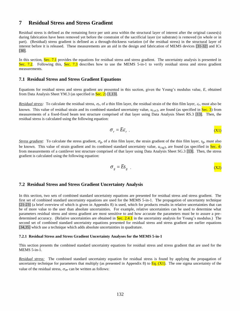
132

7 Residual Stress and Stress Gradient

Residual stress is defined as the remaining force per unit area within the structural layer of interest after the original causes(s)

during fabrication have been removed yet before the constraint of the sacrificial layer (or substrate) is removed (in whole or in

part). (Residual) stress gradient is defined as a through-thickness variation (of the residual stress) in the structural layer of

interest before it is released. These measurements are an aid in the design and fabrication of MEMS devices [31-32] and ICs

[30].

In this section, Sec. 7.1 provides the equations for residual stress and stress gradient. The uncertainty analysis is presented in

Sec. 7.2. Following this, Sec. 7.3 describes how to use the MEMS 5-in-1 to verify residual stress and stress gradient

measurements.

7.1 Residual Stress and Stress Gradient Equations

Equations for residual stress and stress gradient are presented in this section, given the Young’s modulus value, E, obtained

from Data Analysis Sheet YM.3 (as specified in Sec. 2) [1,13].

Residual stress: To calculate the residual stress, r, of a thin film layer, the residual strain of the thin film layer, r, must also be

known. This value of residual strain and its combined standard uncertainty value, ucr3, are found (as specified in Sec. 3) from

measurements of a fixed-fixed beam test structure comprised of that layer using Data Analysis Sheet RS.3 [13]. Then, the

residual stress is calculated using the following equation:

rr E . (X1)

Stress gradient: To calculate the stress gradient, g, of a thin film layer, the strain gradient of the thin film layer, sg, must also

be known. This value of strain gradient and its combined standard uncertainty value, ucsg3, are found (as specified in Sec. 4)

from measurements of a cantilever test structure comprised of that layer using Data Analysis Sheet SG.3 [13]. Then, the stress

gradient is calculated using the following equation:

gg Es . (X2)

7.2 Residual Stress and Stress Gradient Uncertainty Analysis

In this section, two sets of combined standard uncertainty equations are presented for residual stress and stress gradient. The

first set of combined standard uncertainty equations are used for the MEMS 5-in-1. The propagation of uncertainty technique

[21-23] (a brief overview of which is given in Appendix 8) is used, which for products results in relative uncertainties that can

be of more value to the user than absolute uncertainties. For example, relative uncertainties can be used to determine what

parameters residual stress and stress gradient are most sensitive to and how accurate the parameters must be to assure a pre-

determined accuracy. (Relative uncertainties are obtained in Sec. 2.4.1 in the uncertainty analysis for Young’s modulus.) The

second set of combined standard uncertainty equations presented for residual stress and stress gradient are earlier equations

[34,35] which use a technique which adds absolute uncertainties in quadrature.

7.2.1 Residual Stress and Stress Gradient Uncertainty Analyses for the MEMS 5-in-1

This section presents the combined standard uncertainty equations for residual stress and stress gradient that are used for the

MEMS 5-in-1.

Residual stress: The combined standard uncertainty equation for residual stress is found by applying the propagation of

uncertainty technique for parameters that multiply (as presented in Appendix 8) to Eq. (X1). The one sigma uncertainty of the

value of the residual stress, r can be written as follows:

133

22

r

rErr

E

, (X3)

where σE and σεr are the standard deviations of Young’s modulus and residual strain, respectively. Rewriting the above

equation in terms of combined standard uncertainties (by equating σσr with ucr3, E with ucE3, and r with ucr3) results in the

following equation:

2

3

2

3

r

rccEr3rc

u

E

uu

, (X4)

where a number following the subscript “r” in “ucr” and “E” in “ucE” indicates the Young’s modulus data analysis sheet that

is used to obtain these combined standard uncertainty values. Therefore, both ucr3 and ucE3 imply that Data Analysis Sheet

YM.3 is used to obtain these values. However, the number “3” following the subscript “εr” in “ucεr” indicates that Data

Analysis Sheet RS.3 is used to obtain that value. In determining the combined standard uncertainty, a Type B evaluation [21-

23] (i.e., one that uses means other than the statistical Type A analysis) is used for each source of uncertainty.

The expanded uncertainty for residual stress, Ur, is calculated using the following equation:

3rc3rcr ukuU 2 , (X5)


Reporting residual stress results: If it is assumed that the estimated values of the uncertainty components have an approximate

Gaussian distribution with approximate combined standard uncertainty ucr3, the residual stress is believed to lie in the interval

r ucr3 (expansion factor k=1) representing a level of confidence of approximately 68 %.

Stress gradient: The combined standard uncertainty equation for stress gradient is found by applying the propagation of

uncertainty technique for parameters that multiply (as presented in Appendix 8) to Eq. (X2). The one sigma uncertainty of the

value of the stress gradient, g can be written as follows:

22

g

sgEgg

sE

, (X6)

where σE and σsg are the standard deviations of Young’s modulus and strain gradient, respectively. Rewriting the above

equation in terms of combined standard uncertainties (by equating σσg with ucg3, E with ucE3, and σsg with ucsg3) results in the

following equation:

22

g

3csg3cEg3gc

s

u

E

uu , (X7)

where a number following the subscript “g” in “ucg” and “E” in “ucE” indicates the Young’s modulus data analysis sheet that

is used to obtain these combined standard uncertainty values. Therefore, both ucg3 and ucE3 imply that Data Analysis Sheet

YM.3 is used to obtain these values. However, the number “3” following the subscript “sg” in “ucsg” indicates that Data

Analysis Sheet SG.3 is used to obtain that value. In determining the combined standard uncertainty, a Type B evaluation [21-

23] (i.e., one that uses means other than the statistical Type A analysis) is used for each source of uncertainty.

134

The expanded uncertainty for stress gradient, Ug, is calculated using the following equation:

3gc3gcg ukuU 2 , (X8)


Reporting stress gradient results: If it is assumed that the estimated values of the uncertainty components have an approximate

Gaussian distribution with approximate combined standard uncertainty ucg3, the (residual) stress gradient is believed to lie in

the interval g ucg3 (expansion factor k=1) representing a level of confidence of approximately 68 %.

7.2.2 Previous Residual Stress and Stress Gradient Uncertainty Analyses

This section presents previous combined standard uncertainty equations for residual stress and stress gradient.

Residual Stress: A combined standard uncertainty equation that was used previously for residual stress in Data Analysis Sheet

YM.2 [13] is as follows:

2

)(

2

)( rrrE2rc uuu , (X9)

where uE(r) is due to the measurement uncertainty of E and where ur(r) is due to the measurement uncertainty of r. A

number following the subscript “r” in “ucr” indicates the Young’s modulus data analysis sheet that is used to obtain the

combined standard uncertainty value. Therefore, ucr2 implies that Data Analysis Sheet YM.2 is used. In determining the

combined standard uncertainty, a Type B evaluation [21-23] (i.e., one that uses means other than the statistical Type A analysis)

is used for each source of uncertainty. Table X1 gives the equation for both uncertainty components.

The first uncertainty component in Eq. (X9) and listed in Table X1 is uE(r), which is determined from the minimum and

maximum residual stress values (namely, rmin and rmax, respectively). Assuming a Gaussian distribution, uE(r) is calculated

using the equation given in Table X1 where ucE2 is the combined standard uncertainty of the Young’s modulus measurement as

given in Sec. 2.4.2 using Data Analysis Sheet YM.2.

The second uncertainty component in Eq. (X9) and listed in Table X1 is ur(r), which is determined from the minimum and

maximum residual stress values (namely, rmin and rmax, respectively). Assuming a Gaussian distribution, ur(r) is calculated

using the equation in Table X1 where ucr3 is the combined standard uncertainty of the residual strain measurement as given in

Sec 3.4 using Data Analysis Sheet RS.3.

Eq. (X9) can be shown to be equivalent to Eq. (X4) if ucE2 is equated with ucE3 and if the values for Young’s modulus are the

same (in other words if fcorrection is set equal to 0 Hz in Data Analysis Sheet YM.3).

The combined standard uncertainty equation for ucσr1 (obtained using Data Analysis Sheet YM.1 [34,35]) is similar to Eq. (X9),

however the calculation of the first component, uE(σr), uses ucE1 instead of ucE2.

Table X1. Residual Stress Uncertainty Equations [10]

source of uncertainty G or Ua

/ A or Bb

equation

1. uE(r) Young’s modulus G / B

r2cErE uu )(

2. ur(r) residual strain G / B Euu 3rcrr )(



135

Stress gradient: A combined standard uncertainty equation that was used previously for stress gradient in Data Analysis Sheet

YM.2 [13] is as follows:

2

)(

2

)( gsggE2gc uuu , (X10)

where uE(g) is due to the measurement uncertainty of E, and where usg(g) is due to the measurement uncertainty of sg. A

number following the subscript “g” in “ucg” indicates the Young’s modulus data analysis sheet that is used to obtain the

combined standard uncertainty value. Therefore, ucg2 implies that Data Analysis Sheet YM.2 is used. In determining the

combined standard uncertainty, a Type B evaluation [21-23] (i.e., one that uses means other than the statistical Type A analysis)

is used for each source of uncertainty. Table X2 gives the equation for both uncertainty components.

The first uncertainty component in Eq. (X10) and listed in Table X2 is uE(g), which is determined from the minimum and

maximum stress gradient values (namely, gmin and gmax, respectively). Assuming a Gaussian distribution, uE(g) is calculated

using the equation given in Table X2 where ucE2 is the combined standard uncertainty of the Young’s modulus measurement as

given in Sec. 2.4.2 using Data Analysis Sheet YM.2.

The second uncertainty component in Eq. (X10) and listed in Table X2 is usg(g), which is determined from the minimum and

maximum stress gradient values (namely, gmin and gmax, respectively). Assuming a Gaussian distribution, usg(g) is

calculated using the equation given in Table X2 where ucsg3 is the combined standard uncertainty of the strain gradient

measurement as given in Sec. 4.4 using Data Analysis Sheet SG.3.

Eq. (X10) can be shown to be equivalent to Eq. (X7) if ucE2 is equated with ucE3 and if the values for Young’s modulus are the

same (in other words if fcorrection is set equal to 0 Hz in Data Analysis Sheet YM.3).

The combined standard uncertainty equation for ucσg1 (obtained using Data Analysis Sheet YM.1 [34,35]) is similar to Eq.

(X10), however the calculation of the first component, uE(σg), uses ucE1 instead of ucE2.

Table X2. (Residual) Stress Gradient Uncertainty Equations [10]

source of uncertainty G or Ua

/ A or Bb

equation

1. uE(g) Young’s modulus G / B

g2cEgE suu )(

2. usg(g) strain gradient G / B Euu 3csggsg )(



7.3 Using the MEMS 5-in-1 to Verify Residual Stress and Stress Gradient Measurements

To compare your residual stress and stress gradient measurements with NIST measurements, you will need to provide the

optional inputs to Table 4 (in addition to Table 1 and Table 2) in Data Analysis Sheet YM.3. (This data analysis sheet is

accessible via the URL specified in the reference [13], a reproduction of which is given in Appendix 1.) This data analysis sheet

is used for Young’s modulus measurements in Sec. 2. Two inputs to Table 4 (namely, r and ucr3) come from the outputs of

Data Analysis Sheet RS.3 (see Sec. 3) and the other two inputs to Table 4 (namely, sg and ucsg3) come from the outputs of Data

Analysis Sheet SG.3 (see Sec. 4).

Therefore, as specified in Sec. 2.6, to perform the calculations, enter the data into Data Analysis Sheet YM.3 as follows:

1. Press the “Reset this form” button located near the middle of the data analysis sheet. (One of these buttons is

located near the top of the data analysis sheet and the other is located near the middle of the data analysis sheet.)

136

2. Fill out Table 1, Table 2, and Table 4.

3. Press the “Calculate and Verify” button to obtain the results for the cantilever. (One of these buttons is located

near the top of the data analysis sheet and the other is located near the middle of the data analysis sheet.)







specifies an effective residual stress value, r, an effective stress gradient value, g, and their corresponding expanded

uncertainty values, namely Ur and Ug, respectively, (with k=2 in both cases) intending to approximate a 95 % level of


22

)()( rcustomerrrcustomerrr UUD , (X11)

22

)()( gcustomerggcustomergg UUD , (X12)

where Dσr is the absolute value of the difference between your residual stress value, σr(customer), and the residual stress value on

the RM Report of Investigation, σr, and where Uσr(customer) is your expanded uncertainty value and Uσr is the expanded

uncertainty on the RM Report of Investigation. Similarly, Dσg is the absolute value of the difference between your stress

gradient value, σg(customer), and the stress gradient value on the RM Report of Investigation, σg, and where Uσg(customer) is your

expanded uncertainty value and Uσg is the expanded uncertainty on the RM Report of Investigation. If your measured values for

residual stress and stress gradient (as obtained in the newly filled out Data Analysis Sheet YM.3) satisfies your criterion for

acceptance and there are no pertinent “wait” statements at the bottom of your Data Analysis Sheet YM.3, you can consider

yourself to be appropriately measuring residual stress and stress gradient according to the SEMI MS4 Young’s modulus

standard test method [1] according to your criterion for acceptance.

An effective residual stress and an effective stress gradient are reported since an effective Young’s modulus value is used in the

parametric calculations (due to deviations from the ideal geometry and/or composition of the cantilevers as specified in Sec.

2.6). In addition, effective values of residual strain (as specified in Sec. 3.6) and strain gradient (as specified in Sec. 4.6) may

also be used in the calculation of residual stress and stress gradient, respectively. When you use SEMI standard test method

MS4 [1], ASTM standard test method E 2245 [2], and ASTM standard test method E 2246 [3] with your own test structures,

you must be cognizant of the geometry and composition of your test structures because these test methods assume an ideal

geometry and composition, implying that you would be obtaining “effective” values if the geometry and/or composition of your

test structures deviate from the ideal.



137

8 Thickness

Thickness is defined as the height in the z-direction of one or more designated thin-film layers. Step height test structures can

be used to obtain inputs to thickness calculations. Thickness measurements are an aid in the design and fabrication of MEMS

devices [31-32] and ICs [30].

In this section, the NIST-developed thickness test structures on RM 8096 and RM 8097, as shown in Fig. 1 and Figs. 2(a and b)

in the Introduction, are given in Sec. 8.1. Then, Sec. 8.2 discusses the calibration procedure for thickness measurements, Sec.

8.3 discusses the use of Data Analysis Sheet T.1 to obtain the composite oxide beam thickness for RM 8096 chips, and Sec. 8.4

discusses the use of Data Analysis Sheet T.3.a to obtain the poly1 or poly2 thickness for RM 8097 chips. Following this, Sec.

8.5 describes how to use the MEMS 5-in-1 to verify thickness measurements.

8.1 Thickness Test Structures

Thickness measurements for RM 8096, as depicted in Fig. 1, are taken in the fourth grouping of test structures, as shown in Fig.

T1(a). For RM 8097, depicted in Figs. 2(a and b), thickness measurements are taken from the thickness test structures, as shown

in Fig. T1(b), located in the sixth grouping.

(a)

(b) Figure T1. The test structures used for thickness measurements on (a) RM 8096, fabricated on a multi-user 1.5 m CMOS

process [8] followed by a bulk-micromachining etch, as depicted in Fig. 1, and (b) RM 8097, fabricated using a polysilicon

multi-user surface-micromachining MEMS process [9] with a backside etch, as depicted in Figs. 2(a and b).

y

x

y

x

138

For RM 8096: The thickness of the SiO2 beam, tSiO2, is obtained for RM 8096 thickness measurements. This is the thickness of

the composite oxide beam used in Sec. 2 through Sec. 4 for Young’s modulus, residual strain, and strain gradient measurements,

respectively, however, the oxide beam thickness is only a required input for Young’s modulus and residual strain calculations in

Data Analysis Sheet YM.3 and Data Analysis Sheet RS.3, respectively [13]. As shown in Fig. T2, four oxide thicknesses (t1, t2,

t3, and t4) sum together to obtain tSiO2. Fig. T2 also includes a more descriptive nomenclature for these thicknesses as defined

and used in [6].

Before the post-processing of the RM 8096 chips, bulk silicon is directly beneath the bottommost oxide layer of thickness t1 in

Fig. T2. During the post-processing XeF2 etch (as specified in Sec. 1.4.1), any exposed silicon beside the designed cantilevers

and fixed-fixed beams as well as beneath these beams is etched away. Therefore, the bottommost oxide layer in the designed

cantilevers and fixed-fixed beams is of thickness t1, as shown in Fig. T2. Also before the post-processing, a silicon nitride cap

is on top of the topmost oxide layer shown in Fig. T2. During the post-processing CF4+O2 etch (as specified in Sec. 1.4.1), this

nitride cap is removed so that the topmost oxide layer is of thickness t4. Therefore, the oxide beam thickness is comprised of the

four oxide thicknesses given in Fig. T2. Consult [6] for additional specifics associated with the process and these four SiO2

layers.

Figure T2. The four SiO2 thicknesses that comprise the composite oxide beam thickness

There are four distinct thickness test structures (also called step height test structures in Sec. 5) on RM 8096 shown in Fig. T1(a)

(with three occurrences of each structure). The four test structures are given in Fig. T3, from which six step height

measurements are obtained. These six measurements can be used in calculations to determine the thickness of the composite

oxide beams for the determination of Young’s modulus and residual strain in the first and second groupings of test structures (as

specified in Secs. 2 and 3, respectively). The arrow(s) at the top of each test structure locate(s) the step(s) to be measured. As

seen in this figure, one measurement is made on the first and third step height test structures and two measurements are made on

the second and fourth step height test structures in order to obtain the composite beam oxide thickness. The fourth test structure

(associated with the fifth and sixth arrows) does not have a reflective top surface for each platform and as such is intended to be

used with a stylus profilometer (or comparable instrument) as specified in Table T1. (If the stylus makes its initial contact with

the sample surface on top of the oxide between the third and fourth test structures, indentations in the sample surface are not

expected.) Table T1 also includes details associated with the test structures. Cross sections for the test structures shown in Fig.

T3 are given in Fig. T4 through Fig. T7, respectively. The design dimensions for these test structures are given in Table SH1 (in

Sec. 5).

Figure T3. For RM 8096, four step height test structures used to obtain step height measurements.

Measurements from the test structures shown above can be used to determine the thickness of the composite oxide beams.

t1 = tfox(pmd/sub)

t4 = t(gl)

t2 = tpmd(imd/fox)

t3 = timd(gl/pmd) tSiO2 = t1+ t2+ t3+ t4

139

Table T1. For RM 8096, the Measurements and Test Structures Used to Obtain the Composite Oxide Beam Thickness

Measurement #a Test Structure

b Step

c Cross section Measuring

Instrument

1 1st step1AB see Fig. T4 optical interferometer

or comparable instrument

2 2nd

step2rA see Fig. T5 optical interferometer


3 2nd

step1EF see Fig. T5 optical interferometer


4 3rd

step1GH see Fig. T6 optical interferometer


5 4th

step3AB(n)d

see Fig. T7 stylus profilometer


6 4th

step3BC(0) e see Fig. T7 stylus profilometer

or comparable instrument a As given by the arrows in Fig. T3. b Designates one of the four test structures depicted in Fig. T3. c The names of these steps match the names of similar steps in the Certification Plus grouping of test structures on this chip as given in [6].

d The “(n)” indicates this measurement is taken after the chip is post processed using n cycles of a XeF2 etch [6]. The trailing “

” indicates that the

nitride cap has been removed.

e The “(0)” indicates this measurement is taken before the chip is post processed, implying that the nitride cap is still present [6].

The first step height test structure (shown in Fig. T3) is a metal2 (m2)-over-poly1 (p1) step going from active area (aa) to field

oxide (fox) as can be seen in the cross section given in Fig. T4. The name of this step (step1AB) and the other steps in this

grouping of step height test structures are such that they match the names of similar steps for the thickness test structures (given

in the Certification Plus grouping of test structures on this chip) from which the thicknesses of all the layers in the process can

be obtained using the electro-physical technique [6]. Consult the reference [6] for more details.

The reference platform around three of the four sides of this first step height test structure (and the other test structures in Fig.

T3) consists of the deposited oxides sandwiched between active area and metal2.

Figure T4. The cross section of the first step height test structure shown in Fig. T3.

The cross section of the second step height test structure (shown in Fig. T3) from which step2rA and step1EF are obtained is

given in Fig. T5. The cross section of the third step height test structure from which step1GH is obtained is given in Fig. T6.

And, the cross section of the fourth step height test structure from which step3AB(n) is obtained using a stylus profilometer (or

comparable instrument) is given in Fig. T7. This same test structure is used at NIST to obtain step3BC(0) before the chip is post

processed.

140

Figure T5. The cross section of the second step height test structure shown in Fig. T3.

Figure T6. The cross section of the third step height test structure shown in Fig. T3.

Figure T7. The cross section of the fourth step height test structure shown in Fig. T3.

(The label “x” refers to the presence of an oxide and/or nitride layer,

depending upon when the measurement is taken.)

For RM 8097: The poly1 and poly2 thickness test structures are shown in Fig. T1(b) with one of the poly1 cantilevers given in

Fig. T8(a). The poly2 cantilevers have a similar design. To obtain the thickness of this poly1 cantilever (or a poly2 cantilever)

using the optomechanical technique [7], stiction is required. Stiction is defined as the adhesion between the portion of a

structural layer that is intended to be freestanding and its underlying layer. As can be seen in Figs. T8(b and c), the cantilever

beam in Fig. T8(a) is adhered to the top of the underlying layer. (The dimension J in Fig. T8(b) is depicted in Fig. T9 as the

positive vertical distance between the bottom of the suspended structural layer and the top of the underlying layer, which takes

into consideration the roughness of each surface, any residue present between the adhering elements, and a tilting component in

the y-direction.)

z

x

z

x

141

(a)

(b)

(c) Figure T8. For a poly1 cantilever shown in Fig. T1(b), (a) a design rendition,

(b) a cross section showing the cantilever adhered to the top of the underlying layer, and

(c) a 2D data trace [such as Trace a, b, or c in (a)] taken along the length of this cantilever.64

64



Data Trace Exhibiting Stiction

-1

0

1

2

3

4

5

0 0.2 0.4 0.6 0.8 1 1.2

x (mm)

z (

um

) platZplatY

platX

142

Figure T9. A schematic illustration, along the width of the cantilever where it has adhered to the top of the

underlying layer, depicting the component parts of dimension J in Fig. T8(b).

There are two arrays of cantilevers, as can be seen in Fig. T1(b). Table T2 specifies the configurations for these cantilevers.

The top array consists of 15 poly1 cantilevers and the bottom array consists of twelve poly2 cantilevers. As can barely be seen

in this figure, the design length for a cantilever is given next to the second of three iterations of the same length cantilever. Both

the poly1 and the poly2 arrays are designed with poly0 as the underlying layer. This is the layer to which a cantilever exhibiting

stiction adheres. The poly0 layer is designed to encompass an entire array of cantilevers and, to aid in the thickness

measurements, it extends at least 50 m beyond each anchor on the opposite side of the anchor than the side from which the

cantilever extends [as shown in Fig. T8(a) for one cantilever]. As also shown in Fig. T8(a), the anchor is designed to be 50 m

by 50 m in order to obtain a sufficient amount of data in this region.

Table T2. Cantilever Configurations for Thickness Measurements on RM 8097.

Structural Layer Orientation Width

(m)

Length

(m)

Quantity of Beams

poly1 0 20 600, 650, 700, 750, 800 three of each length

(or 15 beams)

poly2 0 20 650, 700, 750, 800 three of each length

(or 12 beams)

There may be instances where the cantilevers in the in-plane length grouping of test structures in Fig. L1(b) would provide

better stiction data than the cantilevers in Fig. T1(b). Therefore, be alert to any comments reflecting this in the applicable data

analysis sheet provided with an RM.

8.2 Calibration Procedures for Thickness Measurements

For RM 8096: On RM 8096, thickness measurements are taken on step height test structures. Therefore, see Sec. 5.2 in the step

height section for calibration in the z-direction.

For RM 8097: On RM 8097, thickness measurements are taken on cantilevers that have adhered to the top of the underlying

layer. In particular, a step height measurement is taken from the top of the poly0 layer to the top of the anchor, preferably using

a stylus profilometer (or comparable instrument). Then, using an optical interferometer (or comparable instrument), a step

height measurement is taken a) from the top of the anchor to the top of the portion of the cantilever that has adhered to the top of

143

the underlying layer and/or b) from the top of the portion of the cantilever that has adhered to the top of the underlying layer to

the top of the underlying layer. For the poly1 (or especially the thinner poly2) layer being examined, measurements should be

taken to ensure the appropriate objective is used such that secondary fringes are not an issue, for example when measuring the

portion of the beam that has adhered to the top of the underlying layer. If secondary fringes are an issue, a higher magnification

objective (e.g., a 50× objective as opposed to a 10× objective) should be used with an appropriate field of view converter.

To calibrate both instruments in the z-direction, see Sec. 5.2 for step height measurements. The NIST-supplied data will use an

optical interferometer for all the thickness measurements to maintain the integrity of the RM since indentations can be created

when the stylus makes contact with the sample surface.

8.3 Using Data Analysis Sheet T.1

Data Analysis Sheet T.1 uses electrical and physical techniques [6] to calculate the thickness of the composite oxide beams on

RM 8096. The electrical techniques use capacitance values for the dielectric layers and sheet resistance and resistivity values

for the metal2 layer. The physical technique is the step height procedure discussed in Sec. 5. Let us look at each of the four

tables given in Data Analysis Sheet T.1 (a reproduction of which is given in Appendix 6) one at a time.

For Table 1 in Appendix 6, the first five step heights [namely, step1AB, step2rA, step1EF, step1GH, and step3AB(n)] in Fig. T4

through Fig. T7 and their combined standard uncertainty values, ucSH, are requested from the four step height test structures

given in Fig. T3. These five values are obtained from Data Analysis Sheet SH.1.a as discussed in Sec. 5. The sixth requested

step height in Table 1 of Appendix 6 is step3BC(0). The NIST-supplied values for step3BC(0) and its combined standard

uncertainty on Data Analysis Sheet T.1, which accompanies RM 8096, should be used since step3BC(0) is a measurement taken

before the post processing. Also requested in Table 1 is a residual one sigma uncertainty component, ures, for each step height.

This component is a place holder to describe additional sources of uncertainty that may become apparent during the

measurement. It can be set equal to zero (i.e., ures=0) such that the combined standard uncertainty value for each step height,

ucstep, is the value obtained from Data Analysis Sheet SH.1.a. In other words:

1acSHresa1cSHcstep uuuu 22

. (T1)

A number (or a number and a letter) following the subscript “SH” in “ucSH” indicates the data analysis sheet that is used to

obtain the combined standard uncertainty value. Therefore, ucSH1a implies that Data Analysis Sheet SH.1.a is used.

At the top of Table 2 in Appendix 6, is requested where is the estimated standard deviation of the value stated for the

permittivity of SiO2, SiO2 (where SiO2=34.5 aF/m). Then, in Table 2, select values of capacitance per unit area (Ca) and their

standard deviations (Ca), as specified in the first column of Table T3, are obtained from the semiconductor fabrication service

[8]. [The NIST-supplied data on Data Analysis Sheet T.1 that accompanies RM 8096 should be used for these entries.] The

corresponding thicknesses (t), as specified in the second column of Table T3, are calculated using the following equation:

aSiO Ct /2 . (T2)

The combined standard uncertainty values for these thicknesses (uctCa) are obtained by applying the propagation of uncertainty

technique (as presented in Appendix 8) to Eq. (T2) for uncorrelated parameters in a multiplicative relationship. The one sigma

uncertainty of the value of the thickness, tCa (which can be equated here with the combined standard uncertainty for the

thickness, uctCa) can be written as follows:

22

2

a

Ca

SiO

tCactCaC

tu

, (T3)

where each uncertainty component is obtained using a Type B analysis. If a residual component is added, the equation can be

written as follows:65

65

This uncertainty equation is different than the one presented in reference [6].

144

222

2

res

resCa

a

Ca

SiO

tCactCarC

tu

, (T4)

where (resCa/rres) represents the relative uncertainty due to a residual component (which is typically assumed to be zero).

Table T3. For RM 8096, the Inputs Requested for Table 2 of Data Analysis Sheet T.1

Obtain

Ca and Ca for the following:

For a calculation of

the corresponding thicknessa using

aSiO Ct /2

p1-to-substrate (sub) tfox(p1/sub)elec

p1-to-aanb tthin(p1/aan)elec

m1-to-sub [tfox,m1(pmd/sub)+tpmd(m1/fox)]elec

m1-to-aan tpmd(m1/aan)elec

m2-to-sub [tfox,m2(pmd/sub)+tpmd(imd/fox)+timd(m2/pmd)]elec

m2-to-aan [tpmd(imd/aan)+timd(m2/pmd)]elec

a Consult the reference [6] for a detailed description of the nomenclature used.

b Poly1-to-active area with an n-implant

For Table 3 in Appendix 6, the metal2 (m2) thickness, t(m2)elec, is calculated using the following equation:

s

elecmR

t

)2( , (T5)

where Rs (the sheet resistance) and (the resistivity) are obtained from the semiconductor fabrication service [8]. [The NIST-

supplied data on Data Analysis Sheet T.1 that accompanies RM 8096 should be used for these entries.] The combined standard

uncertainty value for this thickness (uctRs) is obtained by applying the propagation of uncertainty technique (as presented in

Appendix 8) to Eq. (T5) for uncorrelated parameters in a multiplicative relationship. The one sigma uncertainty of the value of

the thickness, tRs (which can be equated here with the combined standard uncertainty for the thickness, uctRs) can be written as

follows:

22

s

RstRsctRs

Rtu

, (T6)

where Rs (the standard deviation of the sheet resistance) and (the standard deviation of the resistivity) are obtained from the

semiconductor fabrication service [8]. [The NIST-supplied data on Data Analysis Sheet T.1 that accompanies RM 8096 should

be used for these entries.] Each uncertainty component is obtained using a Type B analysis. If a residual component is added,

the equation can be written as follows:66

222

res

resRs

s

RstRsctRs

rRtu

, (T7)

66

This uncertainty equation is different than the one presented in reference [6].

145

where (resRs/rres) represents the relative uncertainty due to a residual component (which is typically assumed to be zero).

To discuss Table 4 in Appendix 6, let us turn our attention to Table T4, which includes the composite oxide beam thickness,

tSiO2, and the four SiO2 thicknesses it is comprised of [namely, tfox(pmd/sub), tpmd(imd/fox), timd(gl/pmd), and t(gl),67

as given by t1, t2,

t3, and t4 as shown in Fig. T2]. Note in Table T4 that t1 can be calculated four different ways as given by t1a, t1b, t1c, and t1d.

This table also includes the equations [6] used to obtain these thicknesses. These equations have been rewritten in this table

using a simplified notation (capital letters) for the thicknesses or step heights as given in Table T5. It is assumed that these

thicknesses or step heights are uncorrelated and that the standard deviations are known. As shown in Table T4, the thickness of

the oxide beam, tSiO2, is given by Z, in the equation that follows:

YXtttttZ 4321SiO2 , (T8)

where

EDCBtttX elecm2/m1imd43 )( , (T9)

and where Y can be calculated in one of the following four possible ways:

MtttY elecm2/m1imd21d1 )( , (T10)

LKAtttY elecimd(m2/m1)21c2 , (T11)

OJAtttY elecimd(m2/m1)21b3 , (T12)

or

OFAtttY elecimd(m2/m1)21a4 , (T13)

where

GI

HIHGO

. (T14)

Table T4. For RM 8096, the Four SiO2 Oxide Thicknesses That Compose the Oxide Beam

Thicknessa Equation

a

1a t1a=tfox(pmd/sub) plus1plus1EF1a tFt1stept

1plus33plus1ABelecsub1pfoxplus1 tHGt1steptt )/(

)/()]/([ )/()/()/( GIHIttt1stept elecaan1pthinelecsub1pfoxelecaan1pthinAB3plus1

so )/( GIHIHGFt1a

1b t1b=tfox(pmd/sub) plus1plus1GH1b tJt1stept

so )/( GIHIHGJt1b

67

Consult the reference [6] for a detailed description of the nomenclature used.

146

1c t1c=tfox(pmd/sub) LKtttt elecaan1mpmdelecfox1mpmdsubpmd1mfox1c )/()/()/(, ][

1d t1d=tfox(pmd/sub) elecpmd2mimdaanimdpmdelecpmd2mimdfoximdpmdsubpmd2mfox1d tttttt ][][ )/()/()/()/()/(,

AM

1 t1 t1 = the thickness (i.e., t1a, t1b, t1c, or t1d) with the smallest value for uc

2 t2=tpmd(imd/fox) elec2/m1mimdelec1m2mimdelecpmd2mimdaanimdpmd2 tAtttt )()/()/()/( ][

3 t3=timd(gl/pmd) elecm2/m1imdelec1m2mimdrABCelec2m3 tDCBt2step03steptt )()/()( )(

4 t4=t(gl) En3stept AB4 )(

tSiO2 Zttttt 43212SiO

a Consult the reference [6] as needed.

Table T5. Simplified Notation for Thicknesses or Step Heights and Their Standard Deviations

Thickness or Step Heighta Simplified

Notation

Standard

Deviation

1 elecpmd2mimdaanimdpmd tt ][ )/()/(

A A

2 elec2mt )(

B B

3 )(03step BC C C

4 rA2step

D D

5 )(n3step AB E E

6 EF1step

F F

7 elecsub1pfoxt )/(

G G

8 AB1step

H H

9 elecaan1pthint )/(

I I

10 GH1step

J J

11 elecfox1mpmdsubpmd1mfox tt ][ )/()/(,

K K

12 elecaan1mpmdt )/(

L L

13 elecpmd2mimdfoximdpmdsubpmd2mfox ttt ][ )/()/()/(,

M M

a Consult the reference [6] as needed.

Table T6 presents these equations for O, X, Y1, Y2, Y3, Y4, and the four possible calculations of Z (namely, Z1, Z2, Z3, and Z4)

along with the equations to calculate the standard deviation values. (Table 4 in Appendix 6 provides the calculation results.)

For all of the standard deviation calculations (except for O), the propagation of uncertainty technique [21-23] (a brief overview

of which is given in Appendix 8) is used for uncorrelated parameters in an additive relationship.

147

Table T6. Standard Deviations for Select Calculations

Thickness

or Step Height

Standard deviation

1

GI

HIHGO

2

4

22

2

22

2

2 )(

)(

)()(1 IHGO

GI

GH

GI

G

GI

HI

2 EDCBX 2222

EDCBX

3 MY1 M1Y

4 LKAY2 222

LKA2Y

5 OJAY3 222

OJA3Y

6 OFAY4 222

OFA4Y

7 11 YXZ

22

1YX1Z

22222

MEDCB1Z

8 22 YXZ

22

2YX2Z

2222222

LKEDCBA2Z

9 33 YXZ

22

3YX3Z

2222222

OJEDCBA3Z

10 44 YXZ

22

4YX4Z

2222222

OFEDCBA4Z

The equation for O [see Eq. (T14)] contains what we are assuming are uncorrelated input parameters in a relationship that is not

solely additive or multiplicative. Therefore, as given in Appendix 8, the partial derivatives are found such that O can be

calculated as follows:

2

2

2

2

2

2

IHGOI

O

H

O

G

O

, (T15)

where

2)(1

GI

HI

G

O

, (T16)

GI

G

H

O

, (T17)

and

2)( GI

GH

I

O

, (T18)

148

so that

2

4

22

2

22

2

2 )(

)(

)()(1 IHGO

GI

GH

GI

G

GI

HI

. (T19)

After equating Z1,Z2,Z3, andZ4 in Table T6 with uZ1, uZ2, uZ3, and uZ4, respectively, the smallest of the combined standard

uncertainty values uZ1, uZ2, uZ3, and uZ4 is called ucSiO2. The corresponding Z value (namely, Z1, Z2, Z3, or Z4, respectively) is

chosen to represent tSiO2.

For RM 8096 that uses Data Analysis Sheet T.1, the expanded uncertainty is USiO2, as calculated using the following equation:

222 2 cSiOcSiOSiO ukuU , (T20)



Gaussianly distributed with approximate combined standard uncertainty ucSiO2, the composite oxide beam thickness is believed

to lie in the interval tSiO2 ucSiO2 (coverage factor k=1) representing a level of confidence of approximately 68 %.

8.4 Using Data Analysis Sheet T.3.a

Data Analysis Sheet T.3.a uses the optomechanical technique [7] to calculate the poly1 or poly2 thickness on RM 8097 three

different ways to obtain αi, αii, and αiii [shown in Fig. T8(b)]. The thickness (αi, αii, or αiii) with the smallest uncertainty is the

chosen thickness unless one of the thicknesses is preselected to be the chosen thickness.

The optomechanical technique uses a cantilever test structure [such as shown in Fig. T8(a) for poly1] that has adhered to the top

of the underlying poly0 layer, as can be seen in Figs. T8(b and c). ASTM standard test method E 2246 [3] can be used to

determine if the cantilever is exhibiting stiction. Once assured that the cantilever is exhibiting stiction, one, two, or three step

height measurements are made using SEMI standard test method MS2 [4]; therefore, Sec. 5 can be consulted, as appropriate, for

measurement and calculation details.

For the three step height measurements (A, B, and C), data from three 2D data traces are used to calculate A, data from three 2D

data traces are used to calculate B, and data from three 2D data traces are used to calculate C, as shown in Fig. T8(b). However,

for the measurement of C, the three data traces can be perpendicular to those shown in Fig. T8(a).

This technique recommends a stylus measurement for the measurement of A, and an optical measurement for the measurements

of B and C for a lower combined standard uncertainty value than if an optical instrument were used for all three measurements.

The NIST-supplied data will use an optical interferometer for all the measurements to maintain the integrity of the RM since

indentations can be created when the stylus makes contact with the sample surface.

Let us look at each of the seven tables (i.e., Tables 1, 2, 3, 4, 5a, 5b, and 5c) given in Data Analysis Sheet T.3.a (a reproduction

of which is given in Appendix 7) one at a time. In these tables, the trailing N subscript to specific parameters is A when

referring to the measurement of A, B when referring to the measurement of B, and C when referring to the measurement of C.

For Table 1 in Appendix 7, the first two inputs given below are used to specify the environmental conditions:

1. The input tempN (i.e., input #1) specifies the temperature during the measurement.

2. The input relative humidityN (i.e., input #2) specifies the relative humidity during the measurement.

Referring to Fig. T1(b), the next five inputs given below are used to locate the target test structure on RM 8097:68

1. The input mat (i.e., input #3) is used to identify if the target test structure is in the upper poly1 array [that is given

the designation P1 in Fig. T1(b)] or in the lower poly2 array (that is given the designation P2).

68 There may be instances where the cantilevers in the in-plane length grouping of test structures in Fig. L1(b) would provide better stiction data than the

cantilevers in Fig. T1(b). Therefore, be alert to any comments reflecting this in the applicable data analysis sheet provided with an RM.

149

2. The input test structure (i.e., input #4) specifies the test structure to be measured. The upper and lower arrays in

Fig. T1(b) consist of only cantilevers. Therefore, the radio button for cantilever should be selected.

3. The input design length (i.e., input #5) specifies the design length of the target test structure. As can barely be

seen in Fig. T1(b), the design length is specified to the left of the anchor of the second of three identically designed

cantilevers. The possible poly1 and poly2 design lengths are given in Table T2.

4. The input which (i.e., input #6) specifies which cantilever of the given length is the target test structure. Since

there are three instances of each cantilever, the radio button corresponding to “first,” “second,” or “third” is used to

locate the target test structure, where “first” corresponds to the topmost cantilever in the array that has the given

length.

5. The input orient (i.e., input #7) specifies the orientation of the target test structure. The orientation is 0 for all of

the cantilevers in Fig. T1(b).

The next three inputs as given below are for general information and reminders to the user:

1. The input magN (i.e., input #8) specifies the magnification used for the measurement of A, B, or C, as appropriate.

2. The input alignN (i.e., input #9) specifies whether or not the data obtained have been aligned properly [4]. The

purpose of this input is to remind the user to align the test structure, with respect to the optics of the instrument,

before taking a measurement.

3. The input levelN (i.e., input #10) specifies whether or not the data have been leveled. The purpose of this input is

to remind the user to level the data before recording a measurement.

The next nine inputs, in Table 1 of Appendix 7, are associated with the calibration in the z-direction of the instrument(s) used to

measure A, B, and C. (A stylus profilometer is recommended for the measurement of A, and an optical interferometer is

recommended for the measurement of B and/or C; however, the NIST-supplied data use an optical interferometer for all the

measurements to maintain the integrity of the RM since indentations can be created when the stylus makes contact with the

sample surface.) Consult Sec 5.2 for details associated with these inputs which follow:

1. The input certN (i.e., input #11),

2. The input certN (i.e., input #12),

3. The input σ6aveN (i.e., input #13),

4. The input aveNz6 (i.e., input #14),

5. The input σ6sameN (i.e., input #15),

6. The input sameNz6 (i.e., input #16),

7. The input zdriftN (i.e., input #17),

8. The input calzN (i.e., input #18), and

9. The input zlinN (i.e., input #19),

where once again N is A when associated with the measurement of A, B when associated with the measurement of B, and C

when associated with the measurement of C.

The remaining eight inputs in Table 1 of Appendix 7 are associated with the processing of RM 8097. (The NIST-supplied data

on Data Analysis Sheet T.3.a that accompanies RM 8097 can be used for the first five inputs.) A description of the eight

inputs69

is given in Data Analysis Sheet T.3.a [13], a reproduction of which is given in Appendix 7, and repeated below:

1. The input repeat(samp)N (i.e., input #20) specifies the relative step height repeatability standard deviation as

obtained from step height test structures fabricated in a process similar to that used to fabricate the sample.

2. The input H (i.e., input #21) specifies the anchor etch depth, as shown in Fig. T8(b), if known (otherwise input 0.0

µm).

3. The input H (i.e., input #22) specifies the range of the anchor etch depth (if known), otherwise input 0.0 µm.

4. The input Jest (i.e., input #23) is an estimated value for the dimension J (if known) [7], as shown in Fig. T8(b). If

it is not known, 0.0 µm should be inputted.

5. The input ucJest (i.e., input #24) is an estimated value for the combined standard uncertainty of Jest (if known);

otherwise 0.0 µm should be inputted.

6. The input sroughX (i.e., input #25) is the uncalibrated surface roughness of platX, shown in Fig. T8(a), calculated as

the smallest of all the measured values obtained for splatXt1 and splatXt2, as discussed below. (Consult the

Definition of Symbols Section, if needed.) However, if the surfaces of platX, platY, and platZ all have identical

69

Consult the Definition of Symbols section, if needed.

150

compositions, then it is calculated as the smallest of all the values obtained for splatXt1, splatXt2, splatYt1, splatYt2,

splatZt1, and splatZt2 in which case sroughX=sroughY=sroughZ.

7. The input sroughY (i.e., input #26) is the uncalibrated surface roughness of platY, shown in Fig. T8(a), calculated as

the smallest of all the measured values obtained for splatYt1 and splatYt2, as discussed below. (Consult the




8. The input sroughZ (i.e., input #27) is the uncalibrated surface roughness of platZ, shown in Fig. T8(a), calculated as

the smallest of all the measured values obtained for splatZt1 and splatZt2, as discussed below. (Consult the




For Table 2 in Appendix 7, input #28 called Fate of A is used to force the selection of αi, as shown in Fig. T8(b), for the

thickness of the poly1 or poly2 layer (as calculated using A and H). Fate of A can also be used to disregard αi as a possible

thickness or let the software select the thickness (αi, αii, or αiii) by the smallest uncertainty value. If Fate of A is greater than or

equal to zero, the rest of the table should be filled out. In this table, the uncalibrated inputs are requested from platX and platY,

as shown in Fig. T8(a) using SEMI standard test method MS2 [4]. In particular, both the platform height and standard deviation

values are requested from Trace a, Trace b, and Trace c, where the data are leveled and zeroed with respect to the top of the

underlying poly0 layer. Therefore, for the measurements of A taken with a stylus profilometer, the uncalibrated inputs platXa1,

platXb1, platXc1, splatXa1, splatXb1, and splatXc1 are requested from platX and the uncalibrated inputs platYa1, platYb1, platYc1,

splatYa1, splatYb1, and splatYc1 are requested from platY.

For Table 3 in Appendix 7, input #41 called Fate of B is used to force the selection of αii, as shown in Fig. T8(b), for the

thickness of the poly1 or poly2 layer (as calculated using A, B, and Jest). It can also be used to disregard αii as a possible

thickness or let the software select the thickness (αi, αii, or αiii). If Fate of B is greater than or equal to zero, the rest of the table

should be filled out. For the measurements of B taken with an optical interferometer, the uncalibrated inputs platYa2, platYb2,

platYc2, splatYa2, splatYb2, and splatYc2 are requested from platY and the uncalibrated inputs platZa1, platZb1, platZc1, splatZa1,

splatZb1, and splatZc1 are requested from platZ. If an interferometric microscope is used for the measurements of A and B, the

platYt and splatYt data for both measurements can be the same (e.g., platYa1=platYa2 and splatYa1=splatYa2) if the measurements

of platXt, platYt, platZt, and the corresponding standard deviations are obtained from the same data trace.

For Table 4 in Appendix 7, input #54 called Fate of C is used to force the selection of αiii, as shown in Fig. T8(b), for the

thickness of the poly1 or poly2 layer (as calculated using C and Jest). For example, if the anchor etch depth is unknown (making

it difficult to calculate αi) it is typically best to obtain the thickness αiii via a measurement of C. Fate of C can also be used to

disregard αiii as a possible thickness or let the software select the thickness (αi, αii, or αiii). If Fate of C is greater than or equal to

zero, the rest of the table should be filled out. These uncalibrated platform height and standard deviations are taken with an

optical interferometer and the data traces can be taken perpendicular to those shown in Fig. T8(a).

For Table 5a in Appendix 7, calibrated values for Aa, Ab, Ac, Ba, Bb, Bc, Ca, Cb, and Cc are calculated using the following

equations:70

zAt cal1platXt1platYtA )( , (T21)

zBt cal2platYt1platZtB )( , (T22)

zCt cal2platXt2platZtC )( , and (T23)

where t is the data trace (i.e., Trace a, Trace b, or Trace c) being considered. Also, the following standard deviations are

calculated:

70

These equations are similar to those found in Sec. 5 for step height measurements.

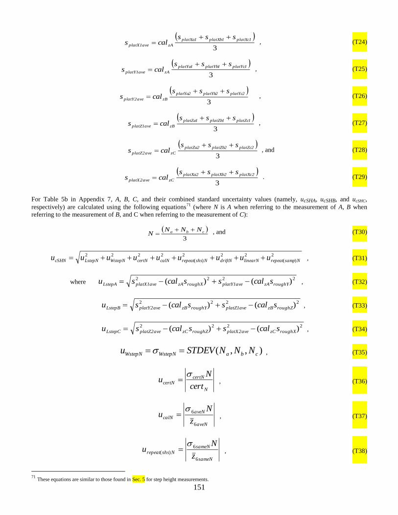
151

3

1platXc1platXb1platXa

zAave1platX

ssscals

, (T24)

3

1platYc1platYb1platYa

zAave1platY

ssscals

, (T25)

3

2platYc2platYb2platYa

zBave2platY

ssscals

, (T26)

3

1platZc1platZb1platZa

zBave1platZ

ssscals

, (T27)

3

2platZc2platZb2platZa

zCave2platZ

ssscals

, and (T28)

3

2platXc2platXb2platXa

zCave2platX

ssscals

. (T29)

For Table 5b in Appendix 7, A, B, C, and their combined standard uncertainty values (namely, ucSHA, ucSHB, and ucSHC,

respectively) are calculated using the following equations71

(where N is A when referring to the measurement of A, B when

referring to the measurement of B, and C when referring to the measurement of C):

3

cba NNNN

, and (T30)

2

)(

222

)(

2222

NsamprepeatlinearNdriftNNshsrepeatcalNcertNWstepNLstepNcSHN uuuuuuuuu , (T31)

where 2222 )()( roughYzAave1platYroughXzAave1platXLstepA scalsscalsu , (T32)

2222 )()( roughZzBave1platZroughYzBave2platYLstepB scalsscalsu , (T33)

2222 )()( roughXzCave2platXroughZzCave2platZLstepC scalsscalsu , (T34)

),,( cbaWstepNWstepN NNNSTDEVu , (T35)

N

certNcertN

cert

Nu

, (T36)

aveN

aveN

calNz

Nu

6

6 , (T37)

sameN

sameN

Nshsrepeatz

Nu

6

6

)(

, (T38)

71

These equations are similar to those found in Sec. 5 for step height measurements.

152

N

zNdriftN

driftNcert

Ncalzu

32

)( , (T39)

3

Nzu linN

linearN , and (T40)

Nu NsamprepeatNsamprepeat )()( . (T41)

Then, in Table 5c of Appendix 7, the following calculations are made [7]:

BACcalc and 22

cSHBcSHAcCcalc uuu , (T42)

HBJ and 22

cHcSHBcJ uuu where 6/HucH , (T43)

HAi and 22

cHcSHAic uuu , (T44)

estcalcii JC and 22

cJestcCcalciic uuu , and (T45)

estiii JC and 22

cJestcSHCiiic uuu . (T46)

The thickness of the suspended poly1 or poly2 layer, , is taken to be the value specified for i, ii, or iii (whichever has the

smallest combined standard uncertainty value, uc) unless the Fate of A, Fate of B, or Fate of C was predetermined in Tables 2,

3, and/or 4, respectively, of Appendix 7. Also, each of the standard uncertainty components is obtained using a Type B

analysis, except for uWstepN, ucalN, urepeat(shs)N, and urepeat(samp)N, which use a Type A analysis.

For RM 8097 using Data Analysis Sheet T.3.a, the expanded uncertainty is U, as calculated using the following equation:

cc ukuU 2 , (T47)



Gaussianly distributed with approximate combined standard uncertainty uc, the thickness is believed to lie in the interval

uc (expansion factor k=1) representing a level of confidence of approximately 68 %.

8.5 Using the MEMS 5-in-1 to Verify Thickness Measurements

To compare your thickness measurements with NIST measurements, you will need to fill out Data Analysis Sheet T.1 or T.3.a

when using RM 8096 or RM 8097, respectively. These data analysis sheets are accessible via the URL specified in the

reference [13], and reproductions of them are given in Appendix 6 and Appendix 7, respectively. After calibrating the

instrument, locating the test structure, taking the measurements, and performing the calculations, the data on your completed

form can be compared with the data on the RM Report of Investigation and the completed data analysis sheet supplied with the

MEMS 5-in-1. Details of the procedure are given below.

153

Calibrate the instrument: Calibrate the instrument(s) as given in Sec. 8.2. For Data Analysis Sheet T.1, consult Sec. 5.6 for

specifics associated with Data Analysis Sheet SH.1.a. For Data Analysis Sheet T.3.a, see Sec. 8.4 for the inputs requested for

the measurement of A, the measurement of B, and the measurement of C.

Locate the target test structure: For RM 8096, as shown in Fig. 1, thickness measurements are taken on the step height test

structures given in the fourth grouping of test structures, which is shown in Fig. T1(a). For RM 8097, as shown in Figs. 2(a and

b), thickness measurements are taken on the cantilever test structures, as shown in Fig. T1(b), that are located within the

Certification Plus grouping of test structures. The specific test structure to be measured (on RM 8096 or RM 8097) can be

deduced from the data entered on the NIST-supplied Data Analysis Sheet T.1 or T.3.a, respectively, which accompanies the

RM.

For RM 8096, the target test structure in Fig. T1(a) can be found as follows:

1. Five data analysis sheets for step height measurements are used to obtain the first five step height inputs [namely,

step1AB, step2rA, step1EF, step1GH, and step3AB(n)] for Data Analysis Sheet T.1. See Sec. 5.6 for specifics. For

these step height inputs, any one of the three instances of the applicable test structure can be measured. The Data

Analysis Sheet SH.1.a that accompanies the RM may contain the data used to calculate one of these step heights.

Therefore, to locate the specific test structure used for that measurement, consult that data analysis sheet. For the

sixth step height input, namely step3BC(0), the NIST-supplied value is used since this is a measurement taken

before the post-processing.

For RM 8097, see Sec. 8.4 for the inputs to Table 1 of Appendix 7 that are used to locate the target test structure in Fig. T1(b).

Be aware that there may be instances where the cantilevers in the in-plane length grouping of test structures in Fig. L1(b) would

provide better stiction data than the cantilevers in Fig. T1(b). Therefore, be alert to any comments reflecting this in the

applicable data analysis sheet provided with the RM.

Take the measurements: For RM 8096, the first five step heights [namely, step1AB, step2rA, step1EF, step1GH, and step3AB(n) ]

are measured from the four step height test structures in Fig. T3 and inputted in Data Analysis Sheet T.1. Recall that step3AB(n)

is taken with a stylus profilometer (or comparable instrument). Then, the NIST-supplied value for the sixth step height [namely,

step3BC(0)] is inputted since this is a measurement taken before the chip is etched. Also, NIST-supplied data can be used for the

Table 2 and Table 3 inputs. Consult Sec. 8.1 and Sec. 5.6 for the step height measurements taken for Data Analysis Sheet T.1.

For RM 8097, using SEMI standard test method MS2 [4], a stylus profilometer is recommended to measure A, as shown in Fig.

T8(b), using three 2D data traces, as shown in Fig. T8(a); however the stylus measurement should not go beyond the anchor and

on to the cantilever because it could damage the test structure. The data are leveled and zeroed with respect to the top of the

underlying poly0 layer. For Data Analysis Sheet T.3.a, uncalibrated measurements of platXa1, platXb1, platXc1, splatXa1,

splatXb1, and splatXc1 are requested from platX. For platY uncalibrated measurements of platYa1, platYb1, platYc1, splatYa1,

splatYb1, and splatYc1 are requested.

Then, using SEMI standard test method MS2 [4], an optical interferometer is used to measure B, as shown in Fig. T8(b), using

the highest magnification objective that is available and feasible especially if secondary fringes may be an issue. The data are

once again leveled and zeroed with respect to the top of the underlying poly0 layer, and Trace a, Trace b, and Trace c, as shown

in Fig. T8(a) are obtained. For Data Analysis Sheet T.3.a, uncalibrated measurements of platYa2, platYb2, platYc2, splatYa2,

splatYb2, and splatYc2 are requested from platY and for platZ uncalibrated measurements of platZa1, platZb1, platZc1, splatZa1,

splatZb1, and splatZc1 are requested.

An optical interferometer is used to measure C, as shown in Fig. T8(b), using an objective (such as a 50× objective as opposed

to a 10× objective, with an appropriate field of view converter) that is useful if secondary fringes may be an issue (for example,

for a thin poly2 layer). The data are leveled and zeroed with respect to the top of the underlying poly0 layer and three data

traces are obtained along the top of the pegged portion of the beam shown in Fig. T8(b) or perpendicular to the traces shown in

Fig. T8(a). Uncalibrated measurements of platZa2, platZb2, platZc2, splatZa2, splatZb2, and splatZc2 are requested from platZ and

for platX, uncalibrated measurements of platXa2, platXb2, platXc2, splatXa2, splatXb2, and splatXc2 are requested.

The NIST-supplied data on Data Analysis Sheet T.3.a were obtained using an optical interferometer for any measurements taken

of A, B, and C to maintain the integrity of the RM since indentations can be created when the stylus makes contact with the

sample surface.

154

Data Analysis Sheet T.3.a also requests the following process specific data: repeat(samp)N, H, H, Jest, ucJest, sroughX, sroughY,

and sroughZ, of which the first five values can be obtained from the NIST-supplied Data Analysis Sheet T.3.a that accompanies

RM 8097.

Perform the calculations: Enter the data into Data Analysis Sheet T.1 or T.3.a as follows:

1. Press the “Reset this form” button located near the top and/or middle of the data analysis sheet.

2. Supply the appropriate inputs to Tables 1 through 3 for Data Analysis Sheet T.1 and the inputs to Tables 1 through

4 for Data Analysis Sheet T.3.a.

3. Press the “Calculate and Verify” button (also located near the top and/or middle of the data analysis sheet) to

obtain the results.







specifies a thickness value (tSiO2 for RM 8096 and for RM 8097) and the expanded uncertainty (USiO2 for RM 8096 and U for RM 8097) with k=2 intending to approximate a 95 % level of confidence. It is your responsibility to determine an

appropriate criterion for acceptance, such as given below:

2

2

2

)(22)(22 SiOcustomerSiOSiOcustomerSiOSiO UUttD , (T43)

22

)()( UUD customercustomer , (T44)

where DSiO2 is the absolute value of the difference between your composite oxide beam thickness value, tSiO2(customer), and the

thickness value on the RM Report of Investigation, tSiO2, and where USiO2(customer) is your expanded uncertainty value and

USiO2 is the expanded uncertainty on the RM Report of Investigation. Similarly, Dα is the absolute value of the difference

between your poly1 (or poly2) thickness value, α(customer), and the thickness value on the RM Report of Investigation, α, and

where Uα(customer) is your expanded uncertainty value and Uα is the expanded uncertainty on the RM Report of Investigation. If

your measured thickness value (as obtained in the newly filled out Data Analysis Sheet T.1 or T.3.a, respectively) satisfies your

criterion for acceptance and there are no pertinent “wait” statements at the bottom of your Data Analysis Sheet T.1 or T.3.a, you

can consider yourself to be appropriately measuring the composite oxide beam thickness or the poly1 (or poly2) thickness,

respectively, according to the SEMI MS2 standard test method [4] according to your criterion for acceptance.



155

9 Summary

The MEMS 5-in-1 is a reference device sold as a NIST Reference Material (RM) that can be of benefit to MEMS designers,

equipment manufacturers, and IC and MEMS foundry service providers. The purpose of the MEMS 5-in-1 is to allow users to

compare their in-house measurements with NIST measurements using five ASTM and SEMI documentary standard test

methods, thereby validating their use of the standard test methods. The five standard test methods [1-5] are for measuring

Young’s modulus, residual strain, strain gradient, step height, and in-plane length, respectively. Additional measurements for

comparison include residual stress, stress gradient, and beam thickness. (The calculations for residual stress and stress gradient

are provided in the Young’s modulus standard test method and the beam thickness calculations rely upon step height

measurements.) Therefore, eight measurements can be compared using five standard test methods. The calculations are

performed on-line using the data analysis sheets (reproductions of which are given in Appendices 1 through 7) accessible via the

NIST MEMS Calculator Website [13].

In summary, we present the following:

A knowledge base that has been developed for the user to take measurements on the MEMS 5-in-1 and verify them with

NIST measurements.

Therefore, the proven skill set obtained from the proper use of the MEMS 5-in-1:

Enables the user to take similar measurements on similarly (or differently) processed test structures. (When a material

property is extracted from measurements taken on a test structure, the user must have an understanding of the geometry

and composition of the test structure in order to obtain meaningful results. In other words, an “effective” value may be

obtained as opposed to a “true” value if there are deviations from the ideal geometry and/or composition of the test

structure.)

Enables measurements to be meaningfully compared between laboratories on similarly (or differently) processed test

structures where differences among community member’s measurements have been tightened due to the use of a

generally accepted standard test method with the RM used as a tool to verify the proper use of the applicable standard

test method. (Once again, when a material property is extracted from measurements taken on a test structure, the user

must have an understanding of the geometry and composition of the test structure in order to determine whether a “true”

or “effective” value has been obtained.)

From an applications point of view, these measurements can be used:

To trouble-shoot a process, to improve yield and track failure sources to speed development. For example, high values

of residual stress (a MEMS 5-in-1 parameter) lead to failure mechanics in ICs such as electromigration, stress migration,

and delamination. Therefore, this method of characterizing residual stress can be of interest for IC process development

and monitoring.

To characterize or validate a process by providing material and dimensional properties.

To facilitate communications between suppliers and customers.

To calibrate an instrument with measurements traceable to a national standard (i.e., the NIST measurements on the RM).

It should be noted that, for example, other physical step height standards are available with lower uncertainty values and

those would provide a more accurate calibration.

Therefore, the MEMS 5-in-1 (as described in the remaining paragraphs) can be considered a stepping stone that provides the

groundwork for all sorts of comparisons and applications.

There are two RMs available for purchase (RM 8096 and RM 8097). RM 8096 is the MEMS 5-in-1 fabricated on a multi-user

1.5 m CMOS process [8] followed by a bulk-micromachining etch, as shown in Fig. 1. For this RM, the material properties of

the composite oxide layer are measured. RM 8097 is the MEMS 5-in-1 fabricated using a polysilicon multi-user surface-

micromachining MEMS process [9] with a backside etch, as shown in Figs. 2(a and b). For this RM, the material properties of

the first or second polysilicon layer are measured.

Each MEMS 5-in-1 is accompanied by a Report of Investigation, data analysis sheets, the five standard test methods [1-5], and

this NIST Special Publication, SP 260. For a current example of the RM 8096 and 8097 Reports of Investigation (each of which

typically includes the eight NIST measurements for comparison) see the Data and Information Files link on https://www-

s.nist.gov/srmors/view_detail.cfm?srm=8096 and https://www-s.nist.gov/srmors/view_detail.cfm?srm=8097, respectively. The

data analysis sheets that accompany the MEMS 5-in-1 include the raw data used at NIST to obtain the measurements on the

Report of Investigation. In Sec. 2.6, 3.6, 4.6, 5.6, 6.6, 7.3, or 8.5 of this SP 260 for the parameter of interest, the user is

instructed to follow the procedures in the applicable ASTM or SEMI standard test method in the taking of the measurements on

the same test structures that NIST measurements were taken. The user’s measurements can then be compared with the NIST




156

measurements supplied on the RM Report of Investigation (and the data analysis sheets) to facilitate the validation of the use of

the documentary standard test methods.

This SP 260 provides overall use and background information for the MEMS 5-in-1 (RM 8096 and RM 8097). Sec. 1 of this SP

260 provides details associated with the following:

The instruments:

o Specifications for the optical vibrometer, stroboscopic interferometer, or comparable instrument used for

Young’s modulus measurements and a validation procedure for frequency measurements, and

o Specifications for the optical interferometer or comparable instrument used for residual strain, strain gradient,

step height, and in-plane length measurements and a validation procedure for height and length measurements.

The contents of the MEMS 5-in-1:

o For RM 8096, and

o For RM 8097.

The classification of the RM 8096 chips,

The post processing of the RM 8096 and RM 8097 chips,

The pre-package inspection (including the classification of the RM 8097 chips),

The packaging of the MEMS 5-in-1,

NIST measurements taken on the MEMS 5-in-1,

The RM Report of Investigation,

Traceability,

Material available for the MEMS 5-in-1,

Storage and handling,

Measurement conditions and procedures for the customer,

Homogeneity of the RMs,

Stability tests, and

Length of certification.

Then, Sec. 2 through Sec. 6 discuss the test structures, the calibration and measurement procedures, the uncertainty analysis, the

round robin results, and how the user can use the MEMS 5-in-1 to verify their in-house measurements for the following standard

test methods, associated parameters, and data analysis sheets:

SEMI standard test method MS4 for Young’s modulus measurements using Data Analysis Sheet YM.3 (a reproduction

of Data Analysis Sheet YM.3 is given in Appendix 1),

ASTM standard test method E 2245 for residual strain measurements using Data Analysis Sheet RS.3 (a reproduction

of Data Analysis Sheet RS.3 is given in Appendix 2),

ASTM standard test method E 2246 for strain gradient measurements using Data Analysis Sheet SG.3 (a reproduction

of Data Analysis Sheet SG.3 is given in Appendix 3),

SEMI standard test method MS2 for step height measurements using Data Analysis Sheet SH.1.a (a reproduction of

Data Analysis Sheet SH.1.a is given in Appendix 4), and

ASTM standard test method E 2244 for in-plane length measurements using Data Analysis Sheet L.0 (a reproduction of

Data Analysis Sheet L.0 is given in Appendix 5).

Section 7 of this SP 260 provides the user with details concerning residual stress and stress gradient calculations. These

calculations can be performed in Data Analysis Sheet YM.3. And finally, Sec. 8 provides the user with details concerning

thickness calculations. For RM 8096, the electro-physical technique [6] as presented in this section is used with Data Analysis

Sheet T.1 (a reproduction of which is given in Appendix 6). For RM 8097, the optomechanical technique [7] as presented in

this section is used with Data Analysis Sheet T.3.a (a reproduction of which is given in Appendix 7).

The NIST SRM Program Office [19] can be contacted (http://www.nist.gov/srm/) to purchase a MEMS 5-in-1 and

accompanying material.

http://www.nist.gov/srm

157

10 Acknowledgements

Acknowledgments go to Richard A. Allen, Craig D. McGray, and Muhammad Afridi in the Test Structures Subgroup within the

MEMS Measurement Science and Services Project at NIST and to Jason J. Gorman in the Engineering Laboratory. The SEMI

North American MEMS Standards Committee and the ASTM Subcommittee E08.05 on Cyclic Deformation and Fatigue Crack

Formation are also acknowledged.

For supporting this work, acknowledgments go to the Microelectronics Device Integration Group, the Semiconductor and

Dimensional Metrology Division, and the Physical Measurement Laboratory as well as the former Office of Microelectronics

Programs, the former Electronics and Electrical Engineering Laboratory, and the former Semiconductor Electronics Division.

MOSIS and MEMSCAP are thanked for the industry cost-share and engineering support received for the RM 8096 and RM

8097 chips, respectively.

Stefan Leigh (Statistical Engineering Division) is acknowledged for his guidance with respect to the ISO GUM rules concerning

combined standard uncertainties, expanded uncertainties, and for guidance with respect to general statistical practices. Andrew

Rukhin (Statistical Engineering Division) is thanked for his behind the scenes assistance with propagation of uncertainty.

Young-Man Choi (Intelligent Systems Division) is thanked for his FEM simulations of resonating cantilevers for Young’s

modulus measurements.

For reviewing this paper, the following people from NIST are acknowledged: Stefan Leigh, Robert L. Watters, Jr., Theodore D.

Doiron, W. Robert Thurber, and Erik M. Secula.

References

[1] SEMI MS4-0212, “Test Method for Young’s Modulus Measurements of Thin, Reflecting Films Based on the

Frequency of Beams in Resonance,” February 2012, (visit http://www.semi.org for ordering information).

[2] ASTM E08, “E 2245 Standard Test Method for Residual Strain Measurements of Thin, Reflecting Films Using an

Optical Interferometer,” ASTM E 224511, December 2011, (visit http://www.astm.org for ordering information).

[3] ASTM E08, “E 2246 Standard Test Method for Strain Gradient Measurements of Thin, Reflecting Films Using an

Optical Interferometer,” ASTM E 224611, January 2012, (visit http://www.astm.org for ordering information).

[4] SEMI MS2-0212, “Test Method for Step Height Measurements of Thin Films,” February 2012, (visit

http://www.semi.org for ordering information).

[5] ASTM E08, “E 2244 Standard Test Method for In-Plane Length Measurements of Thin, Reflecting Films Using an

Optical Interferometer,” ASTM E 224411, December 2011, (visit http://www.astm.org for ordering information).

[6] J. C. Marshall and P. T. Vernier, “Electro-physical technique for post-fabrication measurements of CMOS process

layer thicknesses,” NIST J. Res., Vol. 112, No. 5, p. 223-256, 2007.

[7] J. C. Marshall, “New Optomechanical Technique for Measuring Layer Thickness in MEMS Processes,” Journal of

Microelectromechanical Systems, Vol. 10, No. 1, pp. 153-157, March 2001.

[8] The URL for the MOSIS Website is http://www.mosis.com. “MOSIS provides access to fabrication of prototype and

low-volume production quantities of integrated circuits…by combining designs from many customers onto multi-

project wafers…decreasing the cost of each design.” The 1.5 m On Semiconductor (formerly AMIS) CMOS process

was used for RM 8096.

[9] The RM 8097 chips were fabricated at MEMSCAP using MUMPs-Plus! (PolyMUMPs with a backside etch). The

URL for the MEMSCAP Website is http://www.memscap.com.

[10] J. Marshall, R. A. Allen, C. D. McGray, and J. Geist, “MEMS Young’s Modulus and Step Height Measurements with

Round Robin Results,” NIST J. Res., Vol. 115, No. 5, p. 303-342, 2010.

[11] J. C. Marshall, R. I. Scace, and W. A. Baylies, “MEMS Length and Strain Round Robin Results with Uncertainty

Analysis,” NISTIR 7291, National Institute of Standards and Technology, January 2006.


http://www.astm.org/




http://www.mosis.com/

http://www.memscap.com/

158

[12] J. C. Marshall, E. M. Secula, and J. Huang, “Round Robin for Standardization of MEMS Length and Strain

Measurements,” SEMI Technology Symposium: Innovations in Semiconductor Manufacturing (STS: ISM),

SEMICON West 2004, San Francisco, CA, July 12-14, 2004.

[13] The data analysis sheets, design files, and details associated with the MEMS 5-in-1 can be found at the MEMS

Calculator Web Site (Standard Reference Database 166) accessible via the National Institute of Standards and

Technology (NIST) Data Gateway (http://srdata.nist.gov/gateway/) with the keyword “MEMS Calculator.”

[14] J. C. Marshall, “MEMS Length and Strain Measurements Using an Optical Interferometer,” NISTIR 6779, National

Institute of Standards and Technology, August 2001.

[15] J. Cassard, J. Geist, M. Gaitan, and D. G. Seiler, “The MEMS 5-in-1 Reference Materials (RM 8096 and 8097),” Proc.

of the IEEE International Conference on Microelectronic Test Structures, ICMTS 2012, San Diego, CA, pp. 211-216,

March 21, 2012.

[16] W. E. May, R. M. Parris, C. M. Beck, J. D. Fassett, R. R. Greenberg, F. R. Guenther, G. W. Kramer, S. A. Wise, T. E.

Gills, J. C. Colbert, R. J. Gettings, and B. R. MacDonald, “Definitions of Terms and Modes Used at NIST for Value-

Assignment of Reference Materials for Chemical Measurements,” NIST SP 260-136 (2000) available at

http://www.nist.gov/srm/publications.cfm.

[17] B. N. Taylor and A. Thompson, “The International System of Units (SI),” NIST Special Publication 330, 2008

Edition, National Institute of Standards and Technology, March 2008.

[18] A. Thompson and B. N. Taylor, “Guide for the Use of the International System of Units (SI),” NIST Special

Publication 811, 2008 Edition, National Institute of Standards and Technology, March 2008.

[19] Contact the NIST SRM Program Office to obtain a MEMS 5-in-1, its Report of Investigation, and accompanying data

analysis sheets by visiting http://www.nist.gov/srm/.

[20] J. M. Cassard, J. Geist, T. V. Vorburger, D. T. Read, and D. G. Seiler, “Standard Reference Materials User’s Guide for

SRM 2494 and 2495: The MEMS 5-in-1, 2011 Edition,” NIST SP 260-174, 2011 Ed., Sept. 2011.

[21] B. N. Taylor and C. E. Kuyatt, “Guidelines for Evaluating and Expressing the Uncertainty of NIST Measurement

Results,” NIST Technical Note 1297, National Institute of Standards and Technology, September 1994.

[22] EUROCHEM / CITAC Guide CG 4, “Quantifying Uncertainty in Analytical Measurement,” Second Edition,

QUAM: 2000.1.

[23] International Organization for Standardization, “Guide to the Expression of Uncertainty in Measurement,” ANSI

/NCSL Z540-2-1997, 1997.

[24] W. Weaver, S. P. Timoshenko, and D. H. Young, Vibration Problems in Engineering, 5th

edition, John Wiley & Sons,

1990.

[25] L. Kiesewetter, J.-M. Zhang, D. Houdeau, and A. Steckenborn, Determination of Young’s moduli of micromechanical

thin films using the resonance method, Sensors and Actuators A, Vol. 35, pp. 153-159, 1992.

[26] Draft International Standard (DIS) ISO 25178-604, Geometrical product specifications (GPS) — Surface texture:

Areal — Part 604: Nominal characteristics of non-contact (coherence scanning interferometric microscopy)

instruments, (International Organization for Standardisation, Geneva).

[27] P. de Groot, “Coherence scanning interferometry,” Optical Measurement of Surface Topography, R. Leach, ed., 1st

Edition, pp 187-208 (Springer Verlag, Berlin, 2011).

[28] F. Chang et al., “Gas-phase silicon micromachining with xenon difluoride,” in Proc. SPIE Symp. Micromach.

Microfab., Austin, TX, 1995, pp. 117-128.


http://www.nist.gov/srm/publications.cfm

http://www.nist.gov/srm/

159

[29] G. T. A. Kovacs, Micromachined Transducers Sourcebook, McGraw-Hill, New York, NY, p. 312, 1998.

[30] J. C. Marshall, D. L. Herman, P. T. Vernier, D. L. DeVoe, and M. Gaitan, “Young’s Modulus Measurements in

Standard IC CMOS Processes using MEMS Test Structures,” IEEE Electron Device Letters, Vol. 28, No. 11, p. 960-

963, 2007.

[31] An Assessment of the US Measurement System: Addressing Measurement Barriers to Accelerate Innovation,

Appendix B, “Case Study – Measurement Needs Technology at Issue: Micro-/Nano-Technology”, (NIST Special

Publication 1048, page 309, 2006).

[32] J. V. Clark, “Electro Micro-Metrology,” Ph.D. dissertation, University of California at Berkeley, Dec. 2005.

[33] MEMS and Nanotechnology Clearinghouse, MEMS and Nanotechnology Exchange,

http://www.memsnet.org/material, (accessed April 12, 2010).


Frequency of Beams in Resonance,” November 2009 (visit http://www.semi.org for ordering information).


Frequency of Beams in Resonance,” November 2007 (visit http://www.semi.org for ordering information).

[36] T. B. Gabrielson, Mechanical-Thermal Noise in Micromachined Acoustic and Vibration Sensors, IEEE Transactions

on Electron Devices, Vol. 40, No. 5. pp. 903-909, May 1993.

[37] P. I. Oden, Gravimetric sensing of metallic deposits using an end-loaded microfabricated beam structure, Sensors and

Actuators B, Vol. 53, pp. 191-196, 1998.

[38] E. M. Lawrence, C. Rembe, MEMS Characterization using New Hybrid Laser Doppler Vibrometer / Strobe Video

System, SPIE Proceedings Vol. 5343, Reliability, Testing, and Characterization of MEMS/MOEMS III, pp. 45-54,

January 2003.


Optical Interferometer,” ASTM E 224505, Annual Book of ASTM Standards, Vol. 03.01, 2006. (Visit

http://www.astm.org for ordering information.)










[43] SEMI MS2-1109, “Test Method for Step Height Measurements of Thin Films,” November 2009, (visit

http://www.semi.org for ordering information).

[44] SEMI MS2-0307, “Test Method for Step Height Measurements of Thin, Reflecting Films Using an Optical

Interferometer,” March 2007, (visit http://www.semi.org for ordering information).

[45] T. V. Vorburger, J. F. Song, T. B. Renegar, and A. Zheng, “NIST Surface Roughness and Step Height Calibrations:

Measurement Conditions and Sources of Uncertainty,” January 23, 2008. (Visit

http://www.nist.gov/pml/div683/grp02/upload/nistsurfcalib.pdf.)

http://www.memsnet.org/material









http://www.nist.gov/pml/div683/grp02/upload/nistsurfcalib.pdf

160

[46] ASTM E42, “E 2530 Standard Practice for Calibrating the Z-Magnification of an Atomic Force Microscope at

Subnanometer Displacement Levels Using Si (111) Monatomic Steps,” Annual Book of ASTM Standards, Vol. 03.06,

2006. (Visit http://www.astm.org for ordering information.)










161

Appendix 1 – Data Analysis Sheet YM.3 as of the Writing of This SP 260

Data Analysis Sheet YM.3

Data analysis sheet for determining the Young's modulus value of a thin film layer

for use with the MEMS 5-in-1 RMs

a)

b)

Figure YM.3.1. For CMOS cantilever a) a design rendition and b) a cross section

To obtain the following measurements, consult SEMI standard test method MS4 entitled

"Test Method for Young's Modulus Measurements of Thin, Reflecting Films Based on the

Frequency of Beams in Resonance."

date (optional) = 05 /

18 / 12

identifying words (optional) = April 7th Data

instrument used (optional) = dual beam laser vibrometer

fabrication facility/process (optional) = 1.5 um CMOS process

Input Sample Data

Calculate and Verify

Data

Reset this form

Clear Outputs

162

test chip name (optional) = RM 8096 Monitor 6106.1

test chip number (optional) = s/n 0001

root filename (optional) =

comments (optional) =

Table 1 - Preliminary INPUTS Description

1 temp= 21.1C the temperature during measurement (should be held constant)

2 relative

humidity= 46

% the relative humidity during measurement (if not known, enter

-1)

3 mag= 20× the magnification

4 mat=

poly1

poly2

SiO2

other

the composition of the thin film layer

5* ρ= 2.2g/cm

3 the density of the thin film layer

6 σρ= 0.05g/cm

3 the one sigma uncertainty of the value of ρ

7* μ= 1.84×10

5 Ns/m

2 the viscosity of the ambient surrounding the cantilever

8* W= 28.0μm the suspended beam width

9* t= 2.5846μm

the thickness of the thin film layer

(as found using Data Sheet T.1 or Data Sheet T.3)

10 σthick= 0.1088μm

the one sigma uncertainty of the value of t

(as found using Data Sheet T.1 or Data Sheet T.3)

11 dgap= 30.0μm

the gap depth (distance between the bottom of the suspended

beam and the underlying layer)

12* Einit= 70GPa

the initial estimate for the Young's modulus value of the thin

film layer

13 finstrument= 102.400000MHz

used for calibrating the time base of the instrument: the

frequency setting for the calibration measurements (or the

manufacturer's specification for the clock frequency)

14 fmeter= 102.399437 MHz


calibrated average frequency of the calibration measurements

(or the calibrated average clock frequency) taken with a

frequency meter

15 meter= 1 Hz used for calibrating the time base of the instrument: the

163

standard deviation of the frequency measurements taken with

the frequency meter

16 ucertf = 0 Hz


certified uncertainty of the frequency measurements as

specified on the frequency meter's certificate

* The five starred entries in this table are required inputs for the calculations in the Preliminary

Estimates Table.

Table 2 - Cantilever

INPUTS Description

17 name= RM cantilever the cantilever name (optional)

18 orient=

0

90

180

270

other

the orientation of the cantilever

19* Lcan= 300μm the suspended cantilever length

20 whichcan=

first

second

third

fourth

fifth

sixth

other

indicates which cantilever on the test chip, where "first"

corresponds to the topmost cantilever in the column or array that

has the specified length?

21 σL= 0.2μm the one sigma uncertainty of the value of Lcan

22 fresol= 1.25Hz

the uncalibrated frequency resolution for the given set of

measurement conditions

23 fmeas1= 24.6425kHz

the first uncalibrated, damped resonance frequency measurement

(or the first uncalibrated, undamped resonance frequency

measurement, for example, if the measurements were performed in

a vacuum)

24 fmeas2= 24.6275kHz

the second uncalibrated, damped resonance frequency measurement

(or the second uncalibrated, undamped resonance frequency

164


a vacuum)

25 fmeas3= 24.64kHz

the third uncalibrated, damped resonance frequency measurement

(or the third uncalibrated, undamped resonance frequency


a vacuum)

26 fcorrection= 0kHz the correction term for the cantilever's resonance frequency

27 σsupport= 0kHz

the uncertainty in the cantilever's resonance frequency due to a non-

ideal support (or attachment conditions)

28 σcantilever= 0kHz

the uncertainty in the cantilever's resonance frequency due to

geometry and/or composition deviations from the ideal

* The starred entry in this table is a required input for the calculations in the Preliminary

Estimates Table.

Table 3 - Fixed-Fixed Beam INPUTS (if cantilever not available)

Description

29 name2= the fixed-fixed beam name (optional)

30 orient2=

0

90

other

the orientation of the fixed-fixed beam

31* Lffb= μm the suspended fixed-fixed beam length

32 whichffb=

first

second

third

fourth

fifth

other

indicates which fixed-fixed beam on the test chip, where

"first" corresponds to the topmost fixed-fixed beam in the

column or array that has the specified length?

33 fffb= kHz the average uncalibrated resonance frequency of the

fixed-fixed beam

* The starred entry in this table is a required input for the calculations in the Preliminary

Estimates Table.

165

Table 4 - Optional INPUTS

For residual stress

calculations: Description

34 εr= -2656.0×10

6

the residual strain of the thin film layer

(as found using ASTM E 2245 and Data Sheet RS.3 for compressive

residual strain)

35 ucεr= 100.32×10

6 the combined standard uncertainty value for residual strain

(as found using Data Sheet RS.3 for compressive residual strain)

For stress gradient

calculations:

36 sg= 890.54m

1

the strain gradient of the thin film layer

(as found using ASTM E 2246 and Data Sheet SG.3)

37 ucsg= 55.56m

1

the combined standard uncertainty value for strain gradient

(as found using Data Sheet SG.3)

Table 5 - Preliminary

ESTIMATES* Description

38 fcaninit= 26.2kHz

= SQRT[Einit t2 / (38.330 ρ Lcan

4)]

(the estimated resonance frequency of the cantilever)

39 fffbinithi= InfinitykHz

= SQRT[Einit t2 / (0.946 ρ Lffb

4)]

(the estimated upper bound for the resonance frequency of

the fixed-fixed beam)

40 fffbinitlo= InfinitykHz

= SQRT[Einit t2 / (4.864 ρ Lffb

4)]

(the estimated lower bound for the resonance frequency of

the fixed-fixed beam)

41 Q= 58.4

= W t2

SQRT(ρ Einit) / (24 μLcan2)

(the estimated Q-factor)

42 pdiff= 0.0037%

={1SQRT[11 / (4 Q2)]}×100 % should be < 2 %

(the estimated percent difference between the damped and

undamped resonance frequency of the cantilever)

* The seven starred inputs in the first three tables are required for the calculations in this table.

Input Sample Data

Calculate Estimates

Data

Reset this form

Clear Outputs


Data

Clear Outputs

166

OUTPUTS:

Table 6 - Frequency calculations: Description

43 calf = 0.99999450

= fmeter / finstrument

(the calibration factor for a frequency measurement)

44 fmeasave= 24.6365kHz

= AVE [fmeas1, fmeas2, fmeas3]calf

(the average calibrated damped resonance frequency of the

cantilever, fdampedave, or the average calibrated undamped

resonance frequency of the cantilever if, for example, the

measurements were performed in a vacuum)

45 fundamped1= 24.6433kHz

= fdamped1 / SQRT[11/(4Q2)] where fdamped1=fmeas1(calf)

(the first calibrated undamped resonance frequency calculated

from the cantilever's first damped resonance frequency

measurement, if applicable)



(the second calibrated undamped resonance frequency

calculated from the cantilever's second damped resonance

frequency measurement, if applicable)



(the third calibrated undamped resonance frequency calculated

from the cantilever's third damped resonance frequency

measurement, if applicable)

48 fundampedave= 24.6374kHz

= AVE [fundamped1, fundamped2, fundamped3]

(the average calibrated undamped resonance frequency of the

cantilever assuming fmeas1, fmeas2, and fmeas3 from the second

table are damped resonance frequencies)

49 σfundamped= 0.0080kHz

= STDEV (fundamped1, fundamped2, fundamped3)

(the one sigma uncertainty of the value of fundampedave assuming

fmeas1, fmeas2, and fmeas3 from the second table are damped

resonance frequencies)

50 fcan= 24.6374kHz

= fundampedave + fcorrection

(the modified resonance frequency of the cantilever for use if

fmeas1, fmeas2, and fmeas3 from the second table are damped


51 fmeasavenew= 24.6365kHz

= fmeasave + fcorrection

(the modified resonance frequency of the cantilever for use if

fmeas1, fmeas2, and fmeas3 from the second table are undamped


167

1. Young's modulus calculation (as obtained from the cantilever assuming clamped-free

boundary

conditions):

a. E = 38.330 ρ fcan2 Lcan

4 / t

2 =

62.1GPa

(Use this value if fmeas1, fmeas2, and fmeas3 in the second table are damped

resonance frequencies.)

b. E = 38.330 ρ fmeasavenew2 Lcan

4 / t

2 =

62.1GPa

(Use this value if fmeas1, fmeas2, and fmeas3 in the second table are undamped

resonance frequencies.)

c. ucE = σE = E SQRT[(σρ/ρ)2 + 4(σfcan/fcan)

2 + 16(σL/Lcan)

2 + 4(σthick/t)

2] =

5.42GPa

*

or σE / E = 0.087 *

where σfcan/fcan = SQRT[(σfundamped/fcan)2 + (σfresol/fcan)

2

+ (σfreqcal/fcan)2+ (σsupport/fcan)

2 + (σcantilever/fcan)

2],

σfresol = fresol calf / [2SQRT(3)],

and σfreqcal = fundampedave [SQRT(σmeter2+ ucertf

2) / fmeter]

σρ/ρ = 0.02272

Type B

σthick/t = 0.04209

Type B

σL/Lcan = 0.00066

Type B

σfundamped/fcan = 0.00032*

Type A

σfresol/fcan = 0.00001

Type B

σfreqcal/fcan = 0.000000010

Type B

σsupport/fcan = 0.000000

Type B

σcantilever/fcan = 0.000000

Type B

*assumes fmeas1, fmeas2, and fmeas3 in the second table are damped resonance frequencies

UE = 2ucE = 10.83

GPa (expanded uncertainty)

3ucE = 16.25

GPa

d. E UE = 51.24

GPa (a lower bound for E)

EUE = 72.90

GPa (an upper bound for E)

(assuming fmeas1, fmeas2, and fmeas3 in the second table are damped resonance

frequencies)

e. Report the results as follows: If it is assumed that the estimated values of the

uncertainty components are approximately Gaussianly distributed with approximate

168

combined standard uncertainty ucE, the Young's modulus value is believed to lie in

the interval E ucE (expansion factor k=1) representing a level of confidence of

approximately 68 %.

2. Young's modulus calculation (as obtained from a fixed-fixed beam...not recommended):

a. Esimple = 4.864 ρ ( fffb calf )2

Lffb4

/ t2

= 0.0

GPa

(as obtained from the fixed-fixed beam assuming simply-

supported boundary conditions for both supports)

b. Eclamped = 0.946 ρ ( fffb calf )2 Lffb

4 / t

2 =

0.0GPa

(as obtained from the fixed-fixed beam assuming

clamped-clamped boundary conditions)

c. E = (Esimple Eclamped) / 2 = 0.0

GPa (use this value, if must)

d. uE = (Esimple Eclamped) / 6 = 0.0

GPa (as obtained from a Type B analysis)

e. Report the results as follows: If it is assumed that the estimated value of the

standard uncertainty, uE, is approximately Gaussianly distributed, the Young's modulus

value is believed to lie in the interval E uE (expansion factor k=1) representing a level of

confidence of approximately 68 %.

Table 7 - Optional OUTPUTS (using E and ucE from the cantilever and assuming fmeas1, fmeas2, and

fmeas3 in the second table are damped resonance frequencies)

For residual stress: Description

52 σr= -164.84MPa

= E εr

(the residual stress of the thin film layer)

53 ucσr= 15.673MPa

= |σr| SQRT[(σE / E)2 + (σεr / εr)

2]

(the combined standard uncertainty value for residual stress

where σεr is equated with ucεr)

54 σσr / |σr|= 0.095 where σσr is equated with ucσr

55 σE / E = 0.087 as obtained from this data sheet

56 σεr / |εr|= 0.038

where σεr is equated with ucεr and where εr and ucεr were obtained from

Data Sheet RS.3

57 2ucσr= 31.345MPa

= Uσr

the expanded uncertainty for residual stress

58 3ucσr= 47.018MPa three times the combined standard uncertainty for residual stress

169

59 σrUσr= -196.19MPa a lower bound for σr

60 σrUσr= -133.50MPa an upper bound for σr

For stress gradient:

61 σg= 55271.8GPa/m

= E sg

(the stress gradient of the thin film layer)

62 ucσg= 5928.43GPa/m

= σg SQRT[(σE / E)2 + (σsg / sg)

2]

(the combined standard uncertainty value for stress gradient

where σsg is equated with ucsg)

63 σσg / σg= 0.107 where σσg is equated with ucσg

64 σE / E = 0.087 as obtained from this data sheet

65 σsg / sg = 0.062

where σsg is equated with ucsg and where sg and ucsg were obtained

from Data Sheet SG.3

66 2ucσg= 11856.8GPa/m

= Uσg

the expanded uncertainty for stress gradient

67 3ucσg= 17785.2GPa/m three times the combined standard uncertainty for stress gradient

68 σgUσg= 43415.0GPa/m a lower bound for σg

69 σg+Uσg= 67128.7GPa/m an upper bound for σg

Modify the input data, given the information supplied in any flagged statement below, if

applicable, then recalculate:

1. ok Please provide inputs to Tables 1 and 2 for calculations using data from a cantilever.

2. ok The value for temp should be between 19.4 C and 21.6 C, inclusive.

3. ok The value for relative humidity (if known) should be between 0 % and 60 %, inclusive.

4. w ait

If applicable, please provide inputs to Table 3, ρ, W, t, and Einit for calculations using

data from a fixed-fixed beam.

5. ok The value for mag should be greater than or equal to 20×.

6. ok The value forρ should be between 1.00 g/cm

3 and 5.00 g/cm

3.

7. ok The value for σρ should be between 0.0 g/cm

3 and 0.10 g/cm

3.

8. ok The value for μ should be between 0.70×10

5 Ns/m

2 and 3×10

5 Ns/m

2.

9. ok The value for W should be greater than t and less than Lcan.

10. w ait If Lffb is inputted, the value for W should be greater than t and less than Lffb.

170

11. ok The value for t should be between 0.000 μm and 10.000 μm.

12. ok The value for σthick should be between 0.0 μm and 0.3 μm.

13. ok Squeeze film damping expected for the cantilever since dgap < W / 3.

14. ok The value for Einit should be between 10 GPa and 300 GPa.

15. ok The values for σmeter and ucertf should be between 0.0 Hz and 25.0 Hz, inclusive.

16. ok The value for Lcan should be between 0 μm and 1000 μm.

17. ok The value for σL should be between 0.0 μm and 2.0 μm.

18. ok The value for fresol should be between 0 Hz and 50 Hz.

19. ok The values for fmeas1, fmeas2, and fmeas3 should be between 5.00 kHz and 300.0 kHz.

20. ok The value for fcorrection should be between -10 kHz and 10 kHz, inclusive.

21. ok The values for σsupport and σcantilever should be between 0 kHz and 10 kHz, inclusive.

22. w ait If inputted, the value for Lffb should be between 0 μm and 1000 μm.

23. w ait If inputted, the value for fffb should be between 5.0 kHz and 1200 kHz.

24. ok

If inputted, the value for εr should be between 4500×106

and 4500×106

and not equal

to 0.0.

25. ok If inputted, the value for ucεr should be between and 300.0×10

6.

26. ok If inputted, the value for sg should be between m

1 and 1500.0m

1.

27. ok If inputted, the value for ucsg should be between m

1 and 100.0m

1.

28. ok The values for fmeas1, fmeas2, and fmeas3 are not within 20 kHz of fcaninit.

29. w ait If inputted, the value for fffb should be between fffbinitlo and fffbinithi.

30. ok The value for pdiff should be between 0 % and 2 %.

31. ok The value for calf should be between 0.9990 and 1.0010.

32. ok The value for σfundamped should be between 0.0 kHz and 0.5 kHz, inclusive.

33. ok The value of E obtained from the cantilever should be within 50 GPa of Einit.

34. ok The value of ucE obtained from the cantilever should be between 0 GPa and 50 GPa.

35. w ait

If applicable, the value of E obtained from the fixed-fixed beam should be within 70

GPa of Einit.

171

36. w ait

If applicable, the value of uE obtained from the fixed-fixed beam should be between 0

GPa and 70 GPa.

Return to Main MEMS Calculator Page.

Email questions or comments to [email protected].

NIST is an agency of the U.S. Commerce Department. The Semiconductor and Dimensional Metrology Division is within the Physical Measurement Laboratory. The MEMS Measurement Science and Services Project is within the Microelectronics Device Integration Group.

Date created: 6/5/2006 Last updated: 5/18/2012

http://pml.nist.gov/test-structures/MEMSCalculator.htm


http://www.nist.gov/

http://www.doc.gov/

http://www.nist.gov/pml/div683/

http://www.nist.gov/pml/

http://www.nist.gov/pml/div683/grp03/mnt.cfm

http://www.nist.gov/pml/div683/grp03/

172

Appendix 2 – Data Analysis Sheet RS.3 as of the Writing of This SP 260

Data Analysis Sheet RS.3

Data analysis sheet for residual strain measurements for use with the MEMS 5-in-1 RMs

Figure RS.3.1. Top view of a fixed-fixed beam used to measure residual strain.

To obtain the following measurements, consult ASTM standard test method E 2245 entitled

"Standard Test Method for Residual Strain Measurements of Thin, Reflecting Films

Using an Optical Interferometer."


18 / 12

identifying words (optional) = March 16th data

instrument used (optional) = interferometer




filename of 3-D data set (optional) =

filename of 2-D data traces (optional) =

Input Sample Data


Data

Reset this form

Clear Outputs

173


Table 1 - Preliminary ESTIMATES Description

1 temp = 21.1°C

temperature during measurement (should be

held constant)

2 relative

humidity = 51

% relative humidity during measurement (if not

known, enter -1)

3 material =

Poly1

Poly2

stacked Poly1 and Poly2

SiO2

SiC-2

SiC-3

other

material

4 t = 2.5846μm beam thickness

5 design length = 200μm design length

6 design width = 40μm

design width

(needed for test structure identification

purposes only)

7 which beam?

first

second

third

fourth

other

indicates which fixed-fixed beam on the test

chip, where "first" corresponds to the topmost

fixed-fixed beam in the column or array that has

the specified length?

8 magnification = 25× magnification

9 orientation =

0

90

other

orientation of the fixed-fixed beam on the chip

10 calx = 1.00293

x-calibration factor (for the given

magnification)

11 rulerx = 253μm maximum field of view in the x-direction for

174

the given magnification (as measured on the

screen of the interferometric microscope)

12 σxcal = 0.333μm

one sigma uncertainty in a ruler measurement

(for the given magnification)

13 xres = 0.394775μm

uncalibrated resolution of the interferometric

microscope in the x-direction (for the given

magnification)

14 caly = 1.00478

y-calibration factor (for the given

magnification)

15 calz = 0.99266

z-calibration factor (for the given

magnification)

16 cert = 4.64μm


used for calibration

17 σcert = 0.006μm

certified one sigma uncertainty of the certified

physical step height standard used for

calibration

18 σ6same = 0.0593μm

maximum of two uncalibrated values (σsame1

and σsame2) where σsame1 is the standard deviation

of six measurements taken at the same location

on the physical step height standard before the

data session and σsame2 is the standard deviation

of six measurements taken at this same location

after the data session

19 z6same= 4.6663μm

uncalibrated average of the six calibration

measurements used to calculate σ6same

20 zdrift = 0.0011μm

uncalibrated drift in the calibration data [i.e.,

the uncalibrated positive difference between the

average of the six measurements taken before

the data session at the same location on the

physical step height standard and the average of

the six measurements taken after the data

session at this same location]

21 zlin = 1%

maximum relative deviation from linearity over

the instrument's total scan range, as quoted by

the instrument manufacturer (typically less than

3 %)

22 zres = 0.001μm

calibrated resolution of the interferometer in the

z-direction

23 σLrepeat(samp)'= 1.1565μm

in-plane length repeatability standard deviation

(for the given magnification of the given

interferometric microscope) as obtained for the

same or a similar type of measurement and

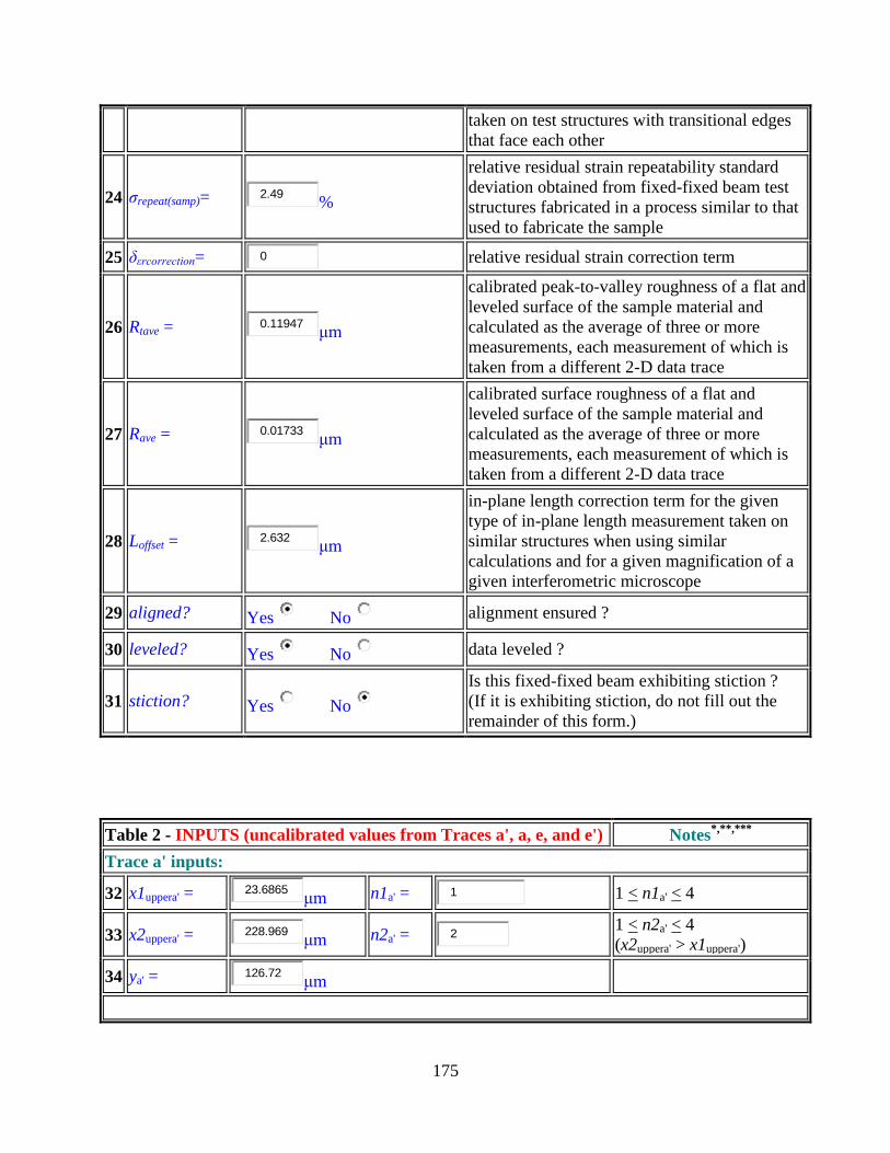
175

taken on test structures with transitional edges

that face each other

24 σrepeat(samp)= 2.49%

relative residual strain repeatability standard

deviation obtained from fixed-fixed beam test

structures fabricated in a process similar to that

used to fabricate the sample

25 δεrcorrection= 0 relative residual strain correction term

26 Rtave = 0.11947μm

calibrated peak-to-valley roughness of a flat and

leveled surface of the sample material and

calculated as the average of three or more

measurements, each measurement of which is

taken from a different 2-D data trace

27 Rave = 0.01733μm

calibrated surface roughness of a flat and





28 Loffset = 2.632μm

in-plane length correction term for the given

type of in-plane length measurement taken on

similar structures when using similar

calculations and for a given magnification of a

given interferometric microscope

29 aligned? Yes No alignment ensured ?

30 leveled? Yes No data leveled ?

31 stiction? Yes No

Is this fixed-fixed beam exhibiting stiction ?

(If it is exhibiting stiction, do not fill out the

remainder of this form.)

Table 2 - INPUTS (uncalibrated values from Traces a', a, e, and e') Notes*,**,***

Trace a' inputs:

32 x1uppera' = 23.6865μm n1a' = 1

1 < n1a' < 4

33 x2uppera' = 228.969μm n2a' = 2

1 < n2a' < 4

(x2uppera' > x1uppera')

34 ya' = 126.72μm

176

Trace a inputs:

35 x1uppera = 23.6865μm n1a = 1

1 < n1a < 4

36 x2uppera = 229.364μm n2a = 2

1 < n2a < 4

(x2uppera > x1uppera)

Trace e inputs:

37 x1uppere = 22.5022μm n1e = 1

1 < n1e < 4

38 x2uppere = 226.601μm n2e = 1

1 < n2e < 4

(x2uppere > x1uppere)

Trace e' inputs:

39 x1uppere' = 22.8969μm n1e' = 1

1 < n1e' < 4

40 x2uppere' = 226.601μm n2e' = 1

1 < n2e' < 4

(x2uppere' > x1uppere')

41 ye' = 25.27μm ya' > ye'

*Where xuppert is the uncalibrated x-value that most appropriately locates the upper corner of the

transitional edge (Edge 1 or Edge 2) using Trace "t"

**The values for n1t and n2t indicate the data point uncertainties associated with the chosen value

for xuppert with the subscript "t" referring to the data trace. In other words, if it is easy to identify

one point that accurately locates the upper corner of the transitional edge, the maximum

uncertainty associated with the identification of this point is ntxrescalx, where nt=1. *Where ya' and ye' are the uncalibrated y-values associated with Traces a' and e', respectively.

Table 3 - INPUTS (uncalibrated values from Trace b) Notes

42 x1F = 30.0029

μm z1F = -0.30069

μm (x1ave < x1F )

43 x2F = 68.296

μm z2F = 2.31704

μm (inflection point)

( x1F < x2F < x3F )

44 x3F = 119.222

μm z3F = 5.47039

μm (most deflected point)

( x1S = x3F ; z1S = z3F )

45 x2S = 175.28

μm z2S = 1.904


46 x3S = 210.02

μm z3S = -0.5755

μm ( x3S < x2ave )

( x1S < x2S < x3S )

177

Table 4 - INPUTS (uncalibrated values from Trace c) Notes

47 x1F = 40.267

μm z1F = 0.232907

μm (x1ave < x1F )

48 x2F = 68.296

μm z2F = 2.51054


( x1F < x2F < x3F )

49 x3F = 121.985

μm z3F = 5.54831


( x1S = x3F ; z1S = z3F )

50 x2S = 175.28

μm z2S = 2.33986


51 x3S = 210.02

μm z3S = -0.40949

μm ( x3S < x2ave )

( x1S < x2S < x3S )

Table 5 - INPUTS (uncalibrated values from Trace d) Notes

52 x1F = 40.267

μm z1F = 0.309133

μm (x1ave < x1F )

53 x2F = 68.296

μm z2F = 2.57527


( x1F < x2F < x3F )

54 x3F = 122.38

μm z3F = 5.59466


( x1S = x3F ; z1S = z3F )

55 x2S = 175.28

μm z2S = 2.11337


56 x3S = 215.152

μm z3S = -0.57715

μm ( x3S < x2ave )

( x1S < x2S < x3S )

Table 6 - OUTPUTS (for in-plane length) Notes

57 x1ave = 23.1930μm = (x1uppera' + x1uppera + x1uppere+ x1uppere' ) / 4

58 x2ave = 227.8838μm = (x2uppera' + x2uppera + x2uppere+ x2uppere' ) / 4

Input Sample Data


Data

Reset this form

Clear Outputs

178

59 Lmeasa' = 205.8840μm = (x2uppera' x1uppera' ) calx

60 Lmeasa = 206.2801μm = (x2uppera x1uppera ) calx

61 Lmease = 204.6968μm = (x2uppere x1uppere ) calx

62 Lmease' = 204.3010μm = (x2uppere' x1uppere' ) calx

63 Lmeas = 205.2905μm = (Lmeasa' + Lmeasa + Lmease + Lmease' ) / 4

64 α =

0.00777radians

0.44511°

= tan–1

[Δx calx / (Δy caly )]

where Δy = ya' – ye' and if (n1a' + n1e' ) < (n2a' + n2e' ) then

Δx = Δx1 = x1uppera'x1uppere'

if (n1a' + n1e' ) > (n2a' + n2e' ) then


65 f = 23.26μm f = x1ave calx

66 l = 228.55μm l = (x2ave calx f) cos(α) + f

67 Laligned = 205.28μm

= aligned length

= lf

68 L = 207.92μm = Laligned + Loffset

69 v1end = 21.94μm

= one endpoint along the v-axis

(the axis parallel to the length of the fixed-fixed beam)

= f Loffset / 2

70 v2end = 229.86μm

= the other endpoint along the v-axis

= l + Loffset / 2

Uncertainty Outputs (for in-plane length):

71 uLL = 0.32993μm

= ( LmaxL − LminL ) / 6

LminL= Lmeasmin cos(α)+Loffset

Lmeasmin = (Lmeasmina'+Lmeasmina

+Lmeasmine+Lmeasmine')/4

Lmeasmint = Lmeast−(n1t+n2t) xres calx

LmaxL= Lmeasmax cos(α)+Loffset

Lmeasmax = (Lmeasmaxa'+Lmeasmaxa

+Lmeasmaxe+Lmeasmaxe')/4

Lmeasmaxt = Lmeast+(n1t+n2t) xres calx

72 uLrepeat(L) = 0.94218μm = σrepeat(L) cos(α)

179

= STDEV(Lmeasa', Lmeasa, Lmease,

Lmease') cos(α)

73 uLxcal = 0.27020μm = ( σxcal / rulerx ) Lmeas cos(α)

74 uLalign = 0.00715μm

= |(Lmaxalign − Lminalign) / (2 SQRT(3))|

where Lmaxalign = Lmeas cos(αmax) + Loffset

and Lminalign = Lmeas cos(αmin) + Loffset

αmin = tan1

[ Δx calx / (Δy caly)

− 2 xres calx / (Δy caly) ]

αmax = tan1

[ Δx calx / (Δy caly)

+ 2 xres calx / (Δy caly) ]

75 uLoffset = 0.87733μm = |Loffset | / 3

76 uLrepeat(samp) = 1.15650

μm =σLrepeat(samp)'

77 ucL = 1.78236μm

= SQRT [uLL2 + uLrepeat(L)

2 + uLxcal

2

+ uLalign2+ uLoffset

2 + uLrepeat(samp)

2]

(Each of the standard uncertainty components is

obtained using a Type B analysis, except for uLrepeat(L)

and uLrepeat(samp), which use a Type A analysis.)

Table 7 - OUTPUTS (for residual strain) Notes

Points Trace b Trace c Trace d

78 g = 30.09μm

40.38μm

40.38μm g = (x1Ft calx f) cos(α) + f

79 h = 68.49μm

68.49μm

68.49μm h = (x2Ft calx f) cos(α) + f

80 i = 119.57μm

122.34μm

122.74μm

i = (x3Ft calx f) cos(α) + f

= (x1St calx f) cos(α) + f

81 j = 175.79μm

175.79μm

175.79μm j = (x2St calx f) cos(α) + f

82 k = 210.63μm

210.63μm

215.78μm k = (x3St calx f) cos(α) + f

83 s =

-1

s = 1 (for downward bending fixed-fixed beams)

s = −1 (for upward bending fixed-fixed beams)

from Trace c

84 AF = 2.91287μm

3.09912μm

3.10434μm use for plotting

85 w1F = 0.25882

0.79183

0.80913 use for plotting

180

86 AS = 3.10592μm

3.19376μm

3.08741μm use for plotting

87 w3S = 5.91306

5.73172

6.10606 use for plotting

88 veF = 70.81270μm

67.55319μm

67.27628μm v-value of first inflection point

89 veS = 171.17945μm

175.88337μm

172.03560μm v-value of second inflection point

90 εr0 = -2135.6822×10

6

-2158.3993×10

6

-2169.5800×10

6

residual strain assuming a zero,

axial-compressive, critical force

91 εrt = -2677.6072×10

6

-2623.5465×10

6

-2666.9612×10

6

residual strain assuming a non-zero,

axial-compressive, critical force

92 εr = -2656.0383 × 10

6

= average residual strain value

from Traces b, c, and d

(USE THIS VALUE)

Table 8 - Preliminary uncertainty OUTPUTS (for residual strain)

93 uW = 28.63781 × 10

6

Trace b Trace c Trace d

94 uLt = 17.11441×10

6

17.04015×10

6

15.49851×10

6

95 uzrest = 0.51766×10

6

0.52226×10

6

0.46116×10

6

96 uxcalt = 6.98460×10

6

6.84381×10

6

6.95997×10

6

97 uxrest = 5.92652×10

6

8.37161×10

6

5.21279×10

6

98 uRavet = 5.17923×10

6

5.22541×10

6

4.61400×10

6

99 unoiset = 30.52395×10

6

30.82681×10

6

27.19112×10

6

100 ucertt = 5.49345×10

6

5.55355×10

6

5.58131×10

6

101 urepeat(shs)t = 53.98698×10

6

54.57763×10

6

54.85046×10

6

102 udriftt = 0.28861×10

6

0.29177×10

6

0.29322×10

6

103 ulineart = 24.52808×10

6

24.79642×10

6

24.92039×10

6

104 ucorrectiont = 0.00000×10

6

0.00000×10

6

0.00000×10

6

105 urepeat(samp)t = 66.67242×10

6

65.32631×10

6

66.40733×10

6

181

106 ucεrt = 100.73447×10

6

100.48540×10

6

99.83772×10

6

Table 9 - Uncertainty OUTPUTS (for residual strain)

Averaging the values from Traces b, c, and d, where applicable

107 uW = 28.63781 × 10

6

due to variations across width of beam (using data

from Traces b, c, and d)

108 uL = 16.55103 × 10

6

due to the measurement uncertainty of L,

but not including uLxcal

109 uzres = 0.50036 × 10

6

due to the resolution of the interferometer in the z-

direction

110 uxcal = 6.92946 × 10

6 due to the calibration in the x-direction

111 uxres = 6.50364 × 10

6

due to the resolution of the interferometric

microscope in the x-direction

112 uRave = 5.00622 × 10

6 due to the sample's surface roughness

113 unoise = 29.51396 × 10

6 due to interferometric noise

114 ucert = 5.54277 × 10

6

due to the uncertainty of the value of the physical

step height standard

115 urepeat(shs) = 54.47169 × 10

6

due to the repeatability of a measurement taken on

the physical step height standard

116 udrift = 0.29120 × 10

6 due to the amount of drift during the data session

117 ulinear = 24.74830 × 10

6 due to the deviation from linearity of the data scan

118 ucorrection = 0.00000 × 10

6

due to the uncertainty of the relative residual strain

correction term

119 urepeat(samp) = 66.13535 × 10

6

due to the uncertainty of residual strain

repeatability measurements

120 ucεr = 100.35253 × 10

6 = (ucεrb + ucεrc + ucεrd) / 3

ucr = SQRT[uW2 + uL

2 + uzres

2 + uxcal

2 + uxres

2 + uRave

2 + unoise

2 + ucert

2

+ urepeat(shs)2 + udrift

2 + ulinear

2 + ucorrection

2 + urepeat(samp)

2 ]

(Each of the standard uncertainty components is obtained using a Type B analysis,

except for uW and urepeat(samp), which use a Type A analysis.)

182

121 ucr = 100.32496× 10

6 combined standard uncertainty

122 2ucr = Ur = 200.64991 × 10

6 expanded uncertainty

123 3ucr = 300.97487 × 10

6

124 εr − Ur = -2856.6882× 10

6 a lower bound for εr

125 εr + Ur = -2455.3884× 10

6 an upper bound for εr

Report the results as follows: If it is assumed that the estimated values of the uncertainty

components are approximately Gaussianly distributed with approximate combined standard

uncertainty ucr, the residual strain is believed to lie in the interval r ucr (expansion factor k=1)

representing a level of confidence of approximately 68%.



1. ok Please fill out the entire form.

2. ok The value for temp should be between 19.4 °C and 21.6 °C, inclusive.


4. ok The value for t should be between 0.000 μm and 10.000 μm.

5. ok The value for the design length should be between 0 μm and 1000 μm.

6. w ait The measured value for L is more than 3ucL from the design length.

7. ok The value for the design width should be between 0 μm and 60 μm.

8. ok Is the magnification appropriate given the design length ?

9. ok Magnifications at or less than 2.5× shall not be used.

10. ok Is 0.95 < calx < 1.05 but not equal to "1"? If not, recheck your x-calibration.

Is 0.95 < caly < 1.05 but not equal to "1"? If not, recheck your y-calibration.

11. ok The value for rulerx should be between 0 μm and 1500 μm.

12. ok The value forσxcal should be between 0 μm and 4 μm.

13. ok The value for xres should be between 0 μm and 2.00 μm.

14. ok Is 0.95 < calz < 1.05 but not equal to "1"? If not, recheck your z-calibration.

15. ok The value for cert should be greater than 0 μm and less than 25 μm.

16. ok The value for σcert should be between 0 μm and 0.100 μm.

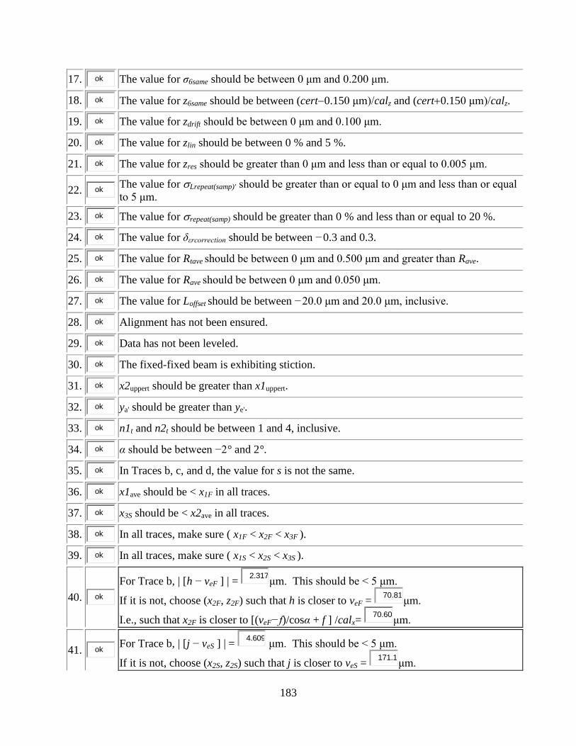
183

17. ok The value for σ6same should be between 0 μm and 0.200 μm.

18. ok The value for z6same should be between (cert0.150 μm)/calz and (cert0.150 μm)/calz.

19. ok The value for zdrift should be between 0 μm and 0.100 μm.

20. ok The value for zlin should be between 0 % and 5 %.

21. ok The value for zres should be greater than 0 μm and less than or equal to 0.005 μm.

22. ok The value for Lrepeat(samp)' should be greater than or equal to 0 μm and less than or equal

to 5 μm.

23. ok The value for repeat(samp) should be greater than 0 % and less than or equal to 20 %.

24. ok The value for δεrcorrection should be between −0.3 and 0.3.

25. ok The value for Rtave should be between 0 μm and 0.500 μm and greater than Rave.

26. ok The value for Rave should be between 0 μm and 0.050 μm.

27. ok The value for Loffset should be between −20.0 μm and 20.0 μm, inclusive.

28. ok Alignment has not been ensured.

29. ok Data has not been leveled.

30. ok The fixed-fixed beam is exhibiting stiction.

31. ok x2uppert should be greater than x1uppert.

32. ok ya' should be greater than ye'.

33. ok n1t and n2t should be between 1 and 4, inclusive.

34. ok α should be between −2° and 2°.

35. ok In Traces b, c, and d, the value for s is not the same.

36. ok x1ave should be < x1F in all traces.

37. ok x3S should be < x2ave in all traces.

38. ok In all traces, make sure ( x1F < x2F < x3F ).

39. ok In all traces, make sure ( x1S < x2S < x3S ).

40. ok

For Trace b, | [h − veF ] | = 2.317

μm. This should be < 5 μm.

If it is not, choose (x2F, z2F) such that h is closer to veF = 70.81

μm.

I.e., such that x2F is closer to [(veF−f)/cosα + f ] /calx= 70.60

μm.

41. ok For Trace b, | [j − veS ] | =

4.609 μm. This should be < 5 μm.

If it is not, choose (x2S, z2S) such that j is closer to veS = 171.1

μm.

185

Appendix 3 – Data Analysis Sheet SG.3 as of the Writing of This SP 260

Data Analysis Sheet SG.3

Data analysis sheet for strain gradient measurements for use with the MEMS 5-in-1 RMs

Figure SG.3.1. Top view of a cantilever test structure used to measure strain gradient.

To obtain the following measurements, consult ASTM standard test method E 2246 entitled

"Standard Test Method for Strain Gradient Measurements of Thin, Reflecting Films



18 / 12







Input Sample Data


Data

Reset this form

Clear Outputs

186

filename of 2-D data traces (optional) =



1 temp = 21.1C


held constant)

2 relative

humidity = 51.0


known, enter -1)

3 material =

Poly1

Poly2


SiO2

SiC-2

SiC-3

other

material


5 design width = 40μm

design width


purposes only)

6 which cantilever?

first

second

third

fourth

fifth

sixth

other

indicates which cantilever on the test chip,

where "first" corresponds to the topmost

cantilever in the column or array that has the

specified length?


8 orientation =

0

90

180

orientation of the cantilever on the chip

187

270

other

9 calx = 1.00293

x-calibration factor (for the given

magnification)

10 rulerx = 253μm

maximum field of view in the x-direction for

the given magnification (as measured on the

screen of the interferometric microscope)

11 σxcal = 0.333μm



12 xres = 0.394775μm



magnification)

13 caly = 1.00478

y-calibration factor (for the given

magnification)

14 calz = 0.99266

z-calibration factor (for the given

magnification)

15 cert = 4.64μm



16 σcert = 0.006μm


physical step height standard used for

calibration

17 σ6same = 0.0593μm

maximum of two uncalibrated values (σsame1

and σsame2) where σsame1 is the standard

deviation of six measurements taken at the

same location on the physical step height

standard before the data session and σsame2 is

the standard deviation of six measurements

taken at this same location after the data

session

18 z6same = 4.6663μm




uncalibrated drift in the calibration data [i.e.,

the uncalibrated positive difference between

the average of the six measurements taken

before the data session at the same location on

the physical step height standard and the

average of the six measurements taken after

the data session at this same location]

20 zlin = 1%

maximum relative deviation from linearity

over the instrument's total scan range, as

quoted by the instrument manufacturer

188

(typically less than 3 %)

21 zres = 0.001μm

calibrated resolution of the interferometer in

the z-direction

22 repeat(samp)= 3.02%

relative strain gradient repeatability standard

deviation as obtained from cantilever test

structures fabricated in a process similar to

that used to fabricate the sample

23 sgcorrection = 0m

1

strain gradient correction term for the given

design length of the cantilever

24 Rtave = 0.11947μm

calibrated peak-to-valley roughness of a flat

and leveled surface of the sample material and




25 Rave = 0.01733μm

calibrated surface roughness of a flat and







28 stiction? Yes No

Is this cantilever exhibiting stiction ?

(If it is exhibiting stiction, do not fill out the

remainder of this form.)

Table 2 - INPUTS (uncalibrated values from Traces a and e)*,**,***

Trace a inputs: Trace e inputs:

29 x1uppert = 8.29027μm

8.29027μm

30 n1t = 1

μm

(for informational purposes only)

2μm

(for informational purposes only)

31 yt = 124.35μm

16.58μm

*Where x1uppert is the uncalibrated x-value that most appropriately locates the upper point of

transitional Edge 1 using Trace "t" **

The values for n1t indicate the data point uncertainty associated with the chosen value for

x1uppert with the subscript "t" referring to the data trace. In other words, if it is easy to identify

one point that accurately locates the upper point of transitional Edge 1, the maximum uncertainty

associated with the identification

of this point is n1txrescalx, where n1t=1. ***

Where yt is the uncalibrated y-value associated with Trace "t" such that ya > ye

189

Table 3 - INPUTS (uncalibrated values from Traces b, c, and d) Notes

Trace b inputs:

32 x1 = 48.9521

μm z1 = -0.08678

μm (x1ave < x1 )

33 x2 = 100.273

μm z2 = 2.91022

μm (x1ave < x2 )

34 x3 = 150.014

μm z3 = 8.11044

μm (x1ave < x3 )

Trace c inputs:

35 x1 = 50.1364

μm z1 = -0.19804

μm (x1ave < x1 )

36 x2 = 100.273

μm z2 = 2.8508

μm (x1ave < x2 )

37 x3 = 150.014

μm z3 = 8.23269

μm (x1ave < x3 )

Trace d inputs:

38 x1 = 51.7155

μm z1 = 0.068687

μm (x1ave < x1 )

39 x2 = 99.0884

μm z2 = 2.94392

μm (x1ave < x2 )

40 x3 = 150.014

μm z3 = 8.22144

μm (x1ave < x3 )

Table 4 - OUTPUTS Notes

41 x1ave = 8.2903μm = (x1uppera + x1uppere) / 2

42 α = 0.00000

radians

0.00000

= tan1

[Δx calx / (Δy caly)]

Δx =x1uppera x1uppere

Δy =ya ye

43 s =

-1from Trace c

s = 1 (for downward bending cantilevers or

if data was taken from the bottom of an upward bending cantilever)

s = −1 (for upward bending cantilevers unless

data was taken from the bottom of an upward bending cantilever)

44 f = 8.3146μm = x1ave calx

Input Sample Data


Data

Reset this form

Clear Outputs

190

Table 5 - OUTPUTS Notes


45 g = 49.0955μm

50.2833μm

51.8670μm = (x1t calxf) cosα + f

46 h = 100.5668μm

100.5668μm


47 i = 150.4535μm

150.4535μm



48 Rint = 1120.91μm

1079.66μm

1171.99μm

Rint is the radius of the circle

describing the shape of the

topmost surface of the cantilever

and (m, n) are the coordinates of

the origin of that circle. These

values are used to plot the function

with the data.

49 m = 10.17μm

10.58 μm

5.36μm

50 n = 1120.15μm

1078.73μm

1171.14μm

51 sgt = 892.1323m

−1

926.2199m

−1

853.2464m

−1 strain gradient

52 sg = 890.5329m

−1

= average strain gradient value

from Traces b, c, and d

(USE THIS VALUE)

Table 6 - Preliminary Uncertainty OUTPUTS

53 uW = 36.5131m

−1


54 uRavet = 4.4489m

−1

4.5504m

−1

4.7082m

−1

55 unoiset = 26.2212m

−1

26.8192m

−1

27.7493m

−1

56 uxcalt = 2.3247m

−1

2.4116m

−1

2.2229m

−1

57 ucertt = 1.1302m

−1

1.1715m

−1

1.0805m

−1

58 urepeat(shs)t = 11.1067m

−1

11.5128m

−1

10.6186m

−1

59 udriftt = 0.0594m

−1

0.0615m

−1

0.0568m

−1

60 ulineart = 5.0462m

−1

5.2307m

−1

4.8244m

−1

191

61 uzrest = 0.4447m

−1

0.4548m

−1

0.4706m

−1

62 uxrest = 11.2180m

−1

11.7428m

−1

11.1434m

−1

63 ucorrectiont = 0.0000m

−1

0.0000m

−1

0.0000m

−1

64 urepeat(samp)t = 26.9424m

−1

27.9718m

−1

25.7680m

−1

65 ucsgt = 55.2086m

−1

56.2210m

−1

55.2804m

−1

Table 7 - Uncertainty OUTPUTS

Averaging the values from Traces b, c, and d, where applicable

66 uW = 36.5131m

−1 due to variations across width of beam

67 uRave = 4.5692m

−1 due to sample's surface roughness

68 unoise = 26.9299m

−1 due to interferometric noise

69 uxcal = 2.3197m

−1 due to calibration in the x-direction

70 ucert = 1.1274m

−1

due to uncertainty of the value of the physical step height

standard

71 urepeat(shs) = 11.0794m

−1

due to the repeatability of a measurement taken on the

physical step height standard

72 udrift = 0.0592m

−1 due to the amount of drift during the data session

73 ulinear = 5.0337m

−1 due to the deviation from linearity of the data scan

74 uzres = 0.4567m

−1

due to the resolution of the interferometer in the z-

direction

75 uxres = 11.3681m

−1

due to the resolution of the interferometric microscope in

the x-direction

76 ucorrection = 0.0000m

−1 due to the uncertainty of the correction term

77 urepeat(samp) = 26.8941m

−1

due to the uncertainty of strain gradient repeatability

measurements

78 ucsgave = 55.5700m

−1 = (ucsgb + ucsgc + ucsgd) / 3

ucsg = SQRT[uW2

+ uRave2 + unoise

2 + uxcal

2 + ucert

2 + urepeat(shs)

2

+ udrift2 + ulinear

2 + uzres

2 + uxres

2 + ucorrection

2 + urepeat(samp)

2]


192

except for uW and urepeat(samp), which use a Type A analysis.)

79 ucsg = 55.5588m

−1 combined standard uncertainty

80 2ucsg = Usg = 111.1176m

−1 expanded uncertainty

81 3ucsg = 166.6764m

−1

82 sg − Usg = 779.4152m

−1 a lower bound for sg

83 sg + Usg = 1001.6505m

−1 an upper bound for sg



uncertainty ucsg, the strain gradient is believed to lie in the interval sg ucsg (expansion factor

k=1) representing a level of confidence of approximately 68%.




2. ok The value for temp should be between 19.4C and 21.6C, inclusive.


4. ok The value for the design length should be between 0 μm and 1000 μm.

5. ok The value for the design width should be between 0 μm and 60 μm.



8. ok Is 0.95 < calx < 1.05 but not equal to "1"? If not, recheck your x-calibration.

Is 0.95 < caly < 1.05 but not equal to "1"? If not, recheck your y-calibration.


10. ok The value for σxcal should be between 0 μm and 4 μm.


12. ok Is 0.95 < calz < 1.05 but not equal to "1"? If not, recheck your z-calibration.

13. ok The value for cert should be greater than 0 μm and less than 25 μm.

14. ok The value for σcert should be between 0 μm and 0.100 μm.

15. ok The value for σ6same should be between 0 μm and 0.200 μm.

193

16. ok The value for z6same should be between (cert 0.150 μm) /calz and (cert + 0.150 μm)

calz.

17. ok The value for zdrift should be between 0 μm and 0.100 μm.

18. ok The value for zlin should be between 0 % and 5 %.

19. ok The value for zres should be greater than 0 μm and less than or equal to 0.005 μm.

20. ok The value for repeat(samp) should be greater than 0 % and less than or equal to 25 %.

21. ok The values for sgt should be greater than 0.0 m

−1, so increase sgcorrection.

22. ok The value for Rtave should be between 0 μm and 0.500 μm and greater than Rave.

23. ok The value for Rave should be between 0 μm and 0.050 μm.



26. ok The cantilever is exhibiting stiction.

27. ok ya should be greater than ye.

28. ok n1t should be between 1 and 4, inclusive.

29. ok α should be between 2 and 2.

30. ok In Trace b, the values of x1, x2, and x3 should be > x1ave.

31. ok In Trace c, the values of x1, x2, and x3 should be > x1ave.

32. ok In Trace d, the values of x1, x2, and x3 should be > x1ave.

33. ok In Traces b, c, and d, the value for s is not the same.








http://www.doc.gov/





194

Appendix 4 – Data Analysis Sheet SH.1.a as of the Writing of This SP 260

Data Analysis Sheet SH.1.a

Data analysis sheet for step height measurements from one step height test structure

for use with the MEMS 5-in-1 RMs

a)

b)

Figure SH.1.a.1. For a CMOS step height test structure: a) a design rendition and b) a cross-

section.

To obtain the following measurements, consult SEMI standard test method MS2 entitled

"Test Method for Step Height Measurements of Thin Films."

Input Sample Data


Data

Reset this form

Clear Outputs

195


18 / 12



fabrication facility (optional) = 1.5 um CMOS process





Table 1 - Preliminary INPUTS

Data Set Prelims Description

1 temp = 21.1°C

temperature during measurement (should be held

constant)

2 relative

humidity = 51.0

% relative humidity during measurement (if not known,

enter -1)

3 proc =

MUMPs

CMOS

other

which process?

4 which =

first

second

third

fourth

fifth

sixth

other

For CMOS RM chips, which of the six step height

measurements?

For MUMPs chips, which quad?

5 which2=

first

second

third

For CMOS chips, which iteration of the test structure

where "first" corresponds to the topmost test structure

in the column?

196

other

NA

6 orient =

0°

90°

180°

270°

other

orientation of the test structure on the test chip

7 mag = 25.0× magnification

8 align = Yes

No

alignment ensured?

9 level = Yes

No

data leveled?

10 cert = 4.640μm

certified value of physical step height standard used

for calibration

11 σcert = 0.006μm


physical step height standard used for calibration

12 σ6ave = 0.0679μm

maximum of two uncalibrated values (σbefore and σafter)

where σbefore is the standard deviation of six

measurements taken across the physical step height

standard before the data session and σafter is the

standard deviation of six measurements taken across

the physical step height standard after the data session

13 z6ave = 4.6969μm


measurements used to calculate σ6ave

14 σ6same= 0.0593μm

maximum of two uncalibrated values (σsame1 and

σsame2) where σsame1 is the standard deviation of six

measurements taken on the physical step height

standard at the same location before the data session

and σsame2 is the standard deviation of six

measurements taken at this same location after the data

session

15 z6same = 4.6663μm




uncalibrated drift in the calibration data (i.e., the

uncalibrated positive difference between the average

of the six measurements taken before the data session

197

at the same location on the physical step height

standard and the average of the six measurements

taken after the data session at this same location)

17 calz = 0.99266 the z-calibration factor (for the given magnification)

18 zlin = 1.0%

if applicable, the maximum relative deviation from

linearity over the instrument's total scan range, as

quoted by the instrument manufacturer (typically less

than 3 %)

19 repeat(samp)= 3.95%

step height relative repeatability standard deviation

obtained from step height test structures fabricated in a

process similar to that used to fabricate the sample

20 sroughNX = 0.0071μm

uncalibrated surface roughness of platNX measured as

the smallest of all the values obtained for

splatNXt. (However, if the surfaces of platNX, platNY,

and platNr all have identical compositions, then it is

measured as the smallest of all the values obtained for

splatNXt, splatNYt, and splatNrDt in which case

sroughNX=sroughNY.)

21 sroughNY = 0.0071μm

uncalibrated surface roughness of platNY measured as

the smallest of all the values obtained for

splatNYt. (However, if the surfaces of platNX, platNY,

and platNr all have identical compositions, then it is

measured as the smallest of all the values obtained for

splatNXt, splatNYt, and splatNrDt in which case

sroughNX=sroughNY.)

Nomenclature:

N refers to the test structure number (1, 2, 3, etc.),

X and Y refer to the platform letter (A, B, C, etc.),

r indicates a reference platform,

D directionally indicates which reference platform, and

t indicates which data trace (a, b, or c).

Input Sample Data


Data

Reset this form

Clear Outputs

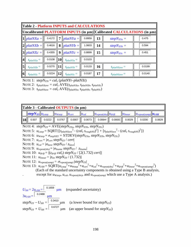
198

Table 2 - Platform INPUTS and CALCULATIONS

Uncalibrated PLATFORM INPUTS (in μm) Calibrated CALCULATIONS (in μm)

1 platNXa = 0.4172 7 platNYa = 0.8959

13 stepNXYa = 0.475

2 platNXb = 0.4616 8 platNYb = 1.0603

14 stepNXYb = 0.594

3 platNXc = 0.4355 9 platNYc = 0.8899

15 stepNXYc = 0.451

4 splatNXa = 0.0108 10 splatNYa = 0.0103

5 splatNXb = 0.0270 11 splatNYb = 0.0133

16 splatNXave = 0.0199

6 splatNXc = 0.0224 12 splatNYc = 0.0187

17 splatNYave = 0.0140

NOTE 1: stepNXYt = calz (platNYtplatNXt)

NOTE 2: splatNXave = calz AVE(splatNXa, splatNXb, splatNXc)

NOTE 3: splatNYave = calz AVE(splatNYa, splatNYb, splatNYc)

Table 3 - Calibrated OUTPUTS (in μm)

stepNXY uLstep uWstep ucert ucal urepeat(shs) udrift ulinear urepeat(samp) ucSH

18 0.507

0.0222

0.0767

0.0007

0.0073

0.00644

0.00003

0.0029

0.0200

0.0829

NOTE 4: stepNXY = AVE(stepNXYa, stepNXYb, stepNXYc)

NOTE 5: uLstep =SQRT{[splatNXave2(calz sroughNX)

2] + [splatNYave

2(calz sroughNY)2]}

NOTE 6: uWstep =σstepNXY = STDEV(stepNXYa, stepNXYb, stepNXYc)

NOTE 7: ucert = |σcert stepNXY / cert|

NOTE 8: ucal = |σ6ave stepNXY / z6ave|

NOTE 9: urepeat(shs) = |σ6same stepNXY / z6same|

NOTE 10: udrift = |(zdrift calz) stepNXY / [2(1.732) cert]|

NOTE 11: ulinear = |zlin stepNXY / (1.732)|

NOTE 12: urepeat(samp) =repeat(samp) |stepNXY|

NOTE 13: ucSH = SQRT(uLstep2+uWstep

2+ucert

2+ucal

2+urepeat(shs)

2+udrift

2+ulinear

2+urepeat(samp)

2)


. except for uWstep, ucal, urepeat(shs), and urepeat(samp) which use a Type A analysis.)

USH = 2ucSH = 0.1659

μm (expanded uncertainty)

3ucSH = 0.2488

μm

stepNXY USH = 0.3410

μm (a lower bound for stepNXY)

stepNXY + USH = 0.6727

μm (an upper bound for stepNXY)

199



uncertainty ucSH, the step height is believed to lie in the interval stepNXY ucSH (expansion factor

k=1) representing a level of confidence of approximately 68%.

Modify the input data, given the information supplied in any flagged statement below, if applicable,

then recalculate:

1. ok Please completely fill out the Preliminary Inputs Table.


3. ok

The value for relative humidity (if known) should be between 0 % and 60 %,

inclusive.

4. ok Is the magnification appropriately greater than 2.5×?



7. ok The value for cert should be between 0.000 μm and 15.000 μm.

8. ok The value for σcert should be between 0.000 μm and 0.100 μm.

9. ok The values for σ6ave and σ6same should be between 0.000 μm and 0.200 μm.

10. ok

The values for z6ave and z6same should be between (cert0.150 μm)/calz and (cert +

0.150 μm)/calz.

11. ok The value for zdrift should be between 0.000 μm and 0.100 μm, inclusive.

12. ok The value for calz should be between 0.900 and 1.100, but not equal to 1.000.

13. ok The value for zlin should be between 0.0 % and 5.0 %, inclusive.

14. ok The value for repeat(samp) should be between 0.0 % and 10.0 %, inclusive.

15. ok

The values for sroughNX and sroughNY should be greater than 0.0 μm and less than or equal

to the smallest measured value for splatNXt and splatNYt, respectively.

16. ok All the platform inputs have not been provided.

17. ok More platform inputs are required for standard deviation calculations.

18. ok The values for platNXt and platNYt should be between 2.500 μm and 2.500 μm.

19. ok The values for splatNXt and splatNYt should be between 0.00 μm and 0.100 μm, inclusive.

20. ok The value for stepNXY should be between 2.500 μm and 2.500 μm.

21. ok The values for uLstep and uWstep should be less than 0.200 μm.

200








http://www.doc.gov/





201

Appendix 5 – Data Analysis Sheet L.0 as of the Writing of This SP 260

Data Analysis Sheet L.0

Data analysis sheet for in-plane length measurements for use with the

MEMS 5-in-1 RMs

Figure L.0.1. Top view of a fixed-fixed beam test structure depicting an example

measurement to be made between Edges 1 and 2.

To obtain the following measurements, consult ASTM standard test method E 2244 entitled,

"Standard Test Method for In-Plane Length Measurements of Thin, Reflecting Films



18 / 12

identifying words (optional) = March 16, 2011 data






filename of 2-D data trace (optional) =


Input Sample Data


Data

Reset this form

Clear Outputs

202


1 temp = 21.1°C


held constant)

2 relative

humidity = 51


known, enter -1)

3 material =

Poly1

Poly2


Metal1

Metal2

SiC-2

SiC-3

other

material

4 type =

Loo

Lii

Lio

Loi

type of measurement:

Loo= outside edge-to-outside edge length

measurement,

Lii = inside edge-to-inside edge length

measurement

Lio= inside edge-to-outside edge length

measurement

Loi = outside edge-to-inside edge length

measurement


6 which?

first

second

third

other

indicates which iteration of the test structure

where "first" corresponds to the topmost or

leftmost test structure in the column or array of

the same material that has the specified length?


8 orientation =

0

90

other

orientation on the chip

9 calx = 1.00293 x-calibration factor (for the given magnification)

203

10 rulerx = 253μm

maximum field of view in the x-direction for the

given magnification (as measured on the screen

of the interferometric microscope)

11 σxcal = 0.333μm



12 xres = 0.394775μm



magnification)

13 caly = 1.004775 y-calibration factor (for the given magnification)

14 calz = 0.99266 z-calibration factor (for the given magnification)

15 Loffset = 2.632μm

in-plane length correction term for the given

magnification of the given interferometric

microscope and associated with a given type of

in-plane length measurement taken on similar

structures when using similar calculations

(If the transitional edges face the same direction,

Loffset=0 μm.)

16 repeat(samp)' = 1.1565μm

in-plane length repeatability standard deviation

(for the given magnification) as obtained from

test structures fabricated in a process similar to

that used to fabricate the sample and for the

same or a similar type of measurement



Table 2 - INPUTS (uncalibrated values) Notes*,**,***,****,*****

Trace a' inputs:

19 x1uppera' = 13.4223μm n1a' = 1

1 < n1a' < 4

20 x2uppera' = 211.204μm n2a' = 1

1 < n2a' < 4

(x2uppera' > x1uppera')

21 ya' = 102.64μm

an outermost data trace

(used in misalignment angle,

α, calculations)

Trace a inputs:

22 x1uppera = 13.4223μm n1a = 1

1 < n1a < 4

204

23 x2uppera = 211.204μm n2a = 1

1 < n2a < 4

(x2uppera > x1uppera)

Trace e inputs:

24 x1uppere = 13.0276μm n1e = 2

1 < n1e < 4

25 x2uppere = 211.204μm n2e = 1

1 < n2e < 4

(x2uppere > x1uppere)

Trace e' inputs:

26 x1uppere' = 13.4223μm n1e' = 1

1 < n1e' < 4

27 x2uppere' = 211.204μm n2e' = 1

1 < n2e' < 4

(x2uppere' > x1uppere')

28 ye' = 78.56μm

an outermost data trace

(used in misalignment angle,

α, calculations)

ya' > ye' *Where xuppert is the uncalibrated x-value that most appropriately locates the upper corner of the

transitional edge (Edge 1 or Edge 2) using Trace "t" **

The values for n1t and n2t indicate the data point uncertainties associated with the chosen value

for xuppert with the subscript "t" referring to the data trace. In other words, if it is easy to identify

one point that accurately locates the upper corner of transitional Edge 1, the maximum

uncertainty associated with the identification of this point is n1txrescalx, where n1t=1. ***

Where ya' and ye' are the uncalibrated y-values associated with Traces a' and e', respectively. ****

Four 2-D data traces are typically used to obtain an in-plane length measurement such that

each trace can be used for both Edge 1 and Edge 2. However, if the measurement is such that

eight 2-D data traces are required (four for Edge 1 and four for Edge 2), call the data traces

associated with Edge 1 a', a, e, and e' and the data traces associated with Edge 2 aa', aa, ee, and

ee'. Therefore, throughout this data sheet, replace x2uppera' with x2upperaa', x2uppera with x2upperaa,

x2uppere with x2upperee, x2uppere' with x2upperee', n2a' with n2aa', n2a with n2aa, n2e with n2ee, and n2e'

with n2ee'. And, if n1a' + n1e' > n2aa' + n2ee', also enter yaa' and yee' in the above table instead of ya'

and ye', respectively.

*****If the transitional edges face the same direction and have similar slopes and magnitudes, the

values locating the lower corner of each transitional edge are entered instead of the upper values,

if the uncertainties associated with the lower corner are typically less than the uncertainties

associated with the upper corner. If this is the case, throughout this data sheet, replace all

occurrences of "upper" with "lower."

Input Sample Data


Data

Reset this form

Clear Outputs

205

Table 3 - OUTPUTS (calibrated values) Equation

29 Lmeasa' = 198.36μm Lmeasa' = (x2uppera' – x1uppera' ) calx

30 Lmeasa = 198.36μm Lmeasa = (x2uppera – x1uppera ) calx

31 Lmease = 198.76μm Lmease = (x2uppere – x1uppere ) calx

32 Lmease' = 198.36μm Lmease' = (x2uppere' – x1uppere' ) calx

33 Lmeas = 198.46μm Lmeas = (Lmeasa' + Lmeasa + Lmease + Lmease')/4

34 α =

0.0000radians

0.0000°

α = tan–1

[Δx calx / (Δy caly )]

where Δy = ya' – ye' and if (n1a' + n1e' ) < (n2a' + n2e' ) then


if (n1a' + n1e' ) > (n2a' + n2e' ) then


35 Lalign = 198.46μm Lalign = Lmeas cos α

36 L = 201.09μm

in plane length

L = Lalign + Loffset

Uncertainty calculations:

37 uL = 0.297μm

uL = ( LmaxL − LminL ) / 6

LminL= Lmeasmin cos(α)+Loffset

Lmeasmin = (Lmeasmina'+Lmeasmina

+Lmeasmine+Lmeasmine') / 4

Lmeasmint = Lmeast− (n1t+n2t) xres calx

LmaxL= Lmeasmax cos(α)+Loffset

Lmeasmax = (Lmeasmaxa'+Lmeasmaxa

+Lmeasmaxe+Lmeasmaxe') / 4

Lmeasmaxt = Lmeast+ (n1t+n2t) xres calx

38 urepeat(L) = 0.198μm

urepeat(L) = σrepeat(L) cos(α)

=STDEV(Lmeasa', Lmeasa, Lmease,

Lmease') cos(α)

39 uxcal = 0.261μm uxcal = (σxcal / rulerx) Lmeas cos(α)

40 ualign = 0.000μm

ualign = |(Lmaxalign – Lminalign)/(2SQRT(3))| ,

with

Lminalign= Lmeas cos(αmin) + Loffset,

Lmaxalign= Lmeas cos(αmax) + Loffset,

αmin = tan–1

[Δx calx / (Δy caly )

– 2xres calx / (Δy caly )] ,

206

αmax = tan–1

[Δx calx / (Δy caly )

+ 2xres calx / (Δy caly )]

41 uoffset = 0.877μm uoffset = |Loffset | / 3

42 urepeat(samp) = 1.157μm urepeat(samp) =repeat(samp)'

43 ucL = 1.517μm

combined standard uncertainty

ucL = SQRT [uL2 + urepeat(L)

2 + uxcal

2

+ ualign2 + uoffset

2 + urepeat(samp)

2]

where each of the standard uncertainty

components is obtained using a Type B analysis,

except for urepeat(L) and urepeat(samp), which use a

statistical Type A analysis

44 2ucL = UL 3.035μm expanded uncertainty

45 3ucL = 4.552μm three times the combined standard uncertainty

46 L – UL = 198.057μm a lower bound for L

47 L + UL = 204.127μm an upper bound for L



uncertainty ucL, the in-plane length is believed to lie in the interval L ucL (expansion factor k=1)

representing a level of confidence of approximately 68%.






4. ok The design length should be between 0 μm and 1050 μm.

5. ok The measured value for L is more than 3ucL from the design length.



8. ok Is 0.95 < calx < 1.05 but not equal to "1" ? If not, recheck your x-calibration.

Is 0.95 < caly < 1.05 but not equal to "1" ? If not, recheck your y-calibration.


207

10. ok The value for σxcal should be between 0 μm and 4 μm.


12. ok Is 0.95 < calz < 1.05 but not equal to "1" ? If not, recheck your z-calibration.

13. ok The value for Loffset should be between –9.0 μm and 9.0 μm, inclusive.

14. ok The value for repeat(samp)' should be between 0 μm and 5 μm, inclusive.



17. ok x2uppert should be greater than x1uppert.

18. ok The measured values for x1uppert should be within 5 μm of their average.

19. ok The measured values for x2uppert should be within 5 μm of their average.

20. ok ya' should be greater than ye'.

21. ok n1t and n2t should be between 1 and 4, inclusive.

22. ok α should be between –2° and 2°.








http://www.doc.gov/





208

Appendix 6 – Data Analysis Sheet T.1 as of the Writing of This SP 260

Data Analysis Sheet T.1

Data analysis sheet for composite oxide thickness measurements in a

commercial CMOS process for use with the MEMS 5-in-1 (RM 8096).

Figure T.1.1. Top view of step height test structures on a MEMS 5-in-1 RM.

To obtain the measurements in this data sheet, consult the following:

[1] J. C. Marshall and P. T. Vernier, "Electro-physical Technique for Post-fabrication

Measurements of CMOS Process Layer Thicknesses," NIST Journal of Research,

Vol. 112, No. 5, 2007, p. 223-256.

[2] SEMI MS2, "Test Method for Step Height Measurements of Thin Films."


18 / 12

identifying words (optional) = March 10th, March 16th, and March 22nd data

instrument(s) used (optional) = interferometer + stylus profilometer




Input Sample Data


Data

Reset this form

Clear Outputs

209

root filename of 3-D data sets (optional) =


TABLE 1 CALIBRATED STEP HEIGHT MEASUREMENTS*

# Step #**

Step***

step height

**** ucSH

**** ures ucstep

*****

(μm) (μm) (μm) (μm)

1 1 H=step1AB 0.507

0.082 0

0.082

2 2 D=step2rA 0.715

0.085

0

0.085

3 3 F=step1EF 0.423

0.067

0

0.067

4 4 J=step1GH -0.405

0.039

0

0.039

5 5 E=step3AB(n) 0.443

0.022

0

0.022

6 6 C=step3BC(0) -0.324

0.018

0

0.018

* Supply inputs to the columns labeled "step height," "ucSH," and "ures."

** The step number as labeled in Fig. T.1.1.

*** The corresponding step for the test structures used with Data Sheet T.2.

**** These inputs can be obtained from Data Sheet SH.1.a.

***** Where ucstep = (ucSH

2 + ures

2)1/2

(where ures is a Type B component that is typically set equal to 0)

TABLE 2 OXIDE THICKNESS VALUES FROM CAPACITANCES*,**

[with σε = 0.1

aF/μm]

#***

Thickness Designation Ca σCa σresCa/rres t uctCa

(aF/μm2) (aF/μm

2) (μm) (μm)

1 G=tfox(p1/sub)elec 36

0.12

0

0.9583

0.0042

2 I=tthin(p1/aan)elec 1106

4.07

0

0.0311

0.0001

6 K=[tfox,m1(pmd/sub)+tpmd(m1/fox)]elec 23

0.09

0

1.5000

0.0073

7 L=tpmd(m1/aan)elec 52

0.40

0

0.6635

0.0055

10 M=[tfox,m2(pmd/sub)+tpmd(imd/fox)

16

0.18

0

2.156

0.025

+timd(m2/pmd)]elec

11 A=[tpmd(imd/aan) +timd(m2/pmd)]elec 27

0.15

0

1.278

0.008

210

* Supply inputs for "Ca," "σCa," "σε," and "σresCa/rres."

** Where t = εSiO2 / Ca with εSiO2 = 34.5 aF/μm

and uctCa = t [(σε / εSiO2)2 + (σCa / Ca)

2 + (σresCa / rres)

2]1/2

where each standard uncertainty component is obtained using a Type B analysis

with σresCa/rres typically set equal to 0. ***

The numbering in this table corresponds to the numbering for the corresponding thicknesses

in Table 2 of Data Sheet T.2.

TABLE 3 THICKNESS VALUES FOR THE INTERCONNECTS*,**

# Symbol Rs σRs ρ σρ σresRs / rres t uctRs

Ω□) Ω□) Ω-μm) Ω-μm) (μm) (μm)

1 B=t(m2)elec 0.0300

0.0014

0.032

0.001

0

1.067

0.060

* Supply inputs to the columns labeled "Rs," "σRs," "ρ," "σρ" and "σresRs / rres."

** Where t = ρ / Rs

and uctRs = t [(σρ / ρ)2

+ (σRs / Rs)2 + (σresRs / rres)

2]

1/2

where each standard uncertainty component is obtained using a Type B analysis

with σresRs/rres typically set equal to 0.

TABLE 4 OXIDE THICKNESS CALCULATION

# Symbol t uc

(μm) (μm)

1 O=GH+HI / (IG) 0.4343

0.0858

2 X=B+CD+E 0.4707

0.1081

3 Y1=M 2.1563

0.0251

4 Y2=A+KL 2.1143

0.0121

5 Y3=AJ+O 2.1171

0.0948

6 Y4=A+F+O 2.1351

0.1093

7 Z1=X+Y1 2.6269

0.1110

8 Z2=X+Y2 2.5850

0.1088

9 Z3=X+Y3 2.5877

0.1438

10 Z4=X+Y4 2.6057

0.1537

11 tSiO2 = 2.5850

ucSiO2 = 0.1088

211

USiO2 = 2ucSiO2 = 0.2176


3ucSiO2 = 0.3264

μm

tSiO2 USiO2 = 2.3674

μm (a lower bound for tSiO2)

tSiO2 USiO2 = 2.8026

μm (an upper bound for tSiO2)



uncertainty ucSiO2, the oxide beam thickness is believed to lie in the interval tSiO2

ucSiO2 (expansion factor k=1) representing a level of confidence of approximately 68 %.


then recalculate:


2. ok

The values for the step heights in Table 1 should be between 2.500 μm and 2.500

μm.

3. ok The ucSH input values in Table 1 should be between 0.0000 μm and 0.2000 μm.

4. ok The values for ures in Table 1 should be between 0.0000 μm and 0.0500 μm, inclusive.

5. ok The value of σε for Table 2 should be between 0.0 aF/μm

and 0.3 aF/μm, inclusive.

6. ok The values for Ca in Table 2 should be between 1.0 aF/μm

2 and 1300.0 aF/μm

2.

7. ok The values for σCa in Table 2 should be between 0.00 aF/μm

2 and 10.00 aF/μm

2.

8. ok The values of σresCa/rres in Table 2 should be between 0 and 0.05, inclusive.

9. ok The value of Rs in Table 3 should be between 0.0100 Ω/□ and 0.0700 Ω/ □.

10. ok The value of σRs in Table 3 should be between 0.0001 Ω/□ and 0.0050 Ω/□.

11. ok The value of ρ in Table 3 should be between 0.020 Ω-μm and 0.040 Ω-μm.

12. ok The value of σρ in Table 3 should be between 0.000 Ω-μm and 0.005 Ω-μm, inclusive.

13. ok The value of σresRs/rres in Table 3 should be between 0 and 0.05, inclusive.

14. ok All of the thicknesses in Table 4 should be between 0.00 μm and 4.00 μm.

15. ok All of the values for uc in Table 4 should be between 0.00 μm and 0.30 μm.





212




http://www.doc.gov/





213

Appendix 7 – Data Analysis Sheet T.3.a as of the Writing of This SP 260

Data Analysis Sheet T.3.a

Data analysis sheet for thickness measurements in a surface-micromachining MEMS

process using an optomechanical technique for use with the MEMS 5-in-1 (RM 8097).

a)

b)

Figure T.3.a.1. For a cantilever test structure a) a design rendition and b) a cross-sectional side

view of a pegged beam.

To obtain the measurements in this data sheet, consult the following:

[1] NIST SP 260-177, "Standard Reference Materials: User's Guide for RM 8096 and 8097:

The MEMS 5-in-1, 2013 Edition"

[2] SEMI MS2, "Test Method for Step Height Measurements of Thin Films."

NOTE: A stylus profilometer is typically used to measure A.

An optical interferometer is typically used to measure B or C.

The platforms are assumed to be reflective with no secondary fringe effect.

If secondary fringes may be an issue, a higher magnification objective (e.g., a 50×

objective) is used with an appropriate field of view converter, if applicable.

214


18 / 12

identifying words (optional) = PolyMUMPs w ith backside etch

instrument(s) used (optional) = interferometer

fabrication facility/process (optional) = MUMPs95

test chip name (optional) = RM 8097 Monitor


filename of data set for the measurement of A (optional) =

filename of data set for the measurement of B (optional) =

filename of data set for the measurement of C (optional) =

comments (optional) = For C, traces w ere taken perpendicular to those in Fig. T.3.a.1.a

Table 1 - Preliminary INPUTS

To Measure:

Description A

B

(optional) C

1 tempN (°C)= 20.6

0

20.6

temperature during measurement

(should be held constant)

2 relative

humidityN (%)= 45.0

0

45.0

relative humidity during measurement

(if not known, enter -1)

3 mat=

poly1

poly2

other

composition of the thin film layer

4 test

structure=

cantilever

fixed-fixed beam

other

test structure being measured

5 design

length (μm)= 800.0

design length


purposes only)

Input Sample Data


Data

Reset this form

Clear Outputs

215

6 which?

first

second

third

other

which test structure on the test chip

where "first" corresponds to the

topmost test structure in the column or

array that has the specified length?

7 orient=

0°

90°

180°

270°

other

orientation of the test structure on the

chip

8 magN (×)= 25.0

0

25.0 magnification

9 alignN= Yes

No

Yes

No

Yes

No

alignment ensured?

10 levelN= Yes

No

Yes

No

Yes

No

data leveled?

11 certN (μm)= 1.0233

0

1.0233

certified value of physical step height

standard used for calibration

12 σcertN (μm)= 0.00265

0

0.00265

certified one sigma uncertainty of the

certified physical step height standard


13 σ6aveN (μm)= 0.0532

0

0.0532

maximum of two uncalibrated values

(σbefore and σafter) where σbefore is the

standard deviation of six

measurements taken across the

physical step height standard before

the data session and σafter is the


measurements taken across the

physical step height standard after the

data session

14 ̅6aveN (μm)= 0.9834

0

0.9834

uncalibrated average of the six

calibration measurements used to

calculate σ6ave

15 σ6sameN (μm)= 0.0917

0

0.0917

maximum of two uncalibrated values

(σsame1 and σsame2) where σsame1 is the


measurements taken on the physical

216

step height standard at the same

location before the data session and

σsame2 is the standard deviation of six

measurements taken at this same

location after the data session

16 ̅6sameN (μm)= 1.0354

0

1.0354

uncalibrated average of the six

calibration measurements used to

calculate σ6same

17 zdriftN (μm)= 0.0008

0

0.0008

uncalibrated drift in the calibration

data (i.e., the uncalibrated positive

difference between the average of the

six measurements taken before the data

session at the same location on the

physical step height standard and the

average of the six measurements taken

after the data session at this same

location)

18 calzN= 1.00888

0

1.00888

the z-calibration factor (for the given

magnification)

19 zlinN (%)= 1.0

0

1.0

if applicable, the maximum relative

deviation from linearity over the

instrument's total scan range, as quoted

by the instrument manufacturer

(typically less than 3 %)

20 σrepeat(samp)N(%)= 7.35

0

7.35

step height relative repeatability

standard deviation obtained from step

height test structures fabricated in a

process similar to that used to fabricate

the sample

21 H (μm)= 0.000

anchor etch depth (if known);

otherwise input 0.0 μm

22 ΔH (μm)= 0.000

range of the anchor etch depth (if

known); otherwise input 0.0 μm

23 Jest (μm)= 0.000

estimated value for the dimension J (if

known); otherwise input 0.0 μm

24 ucJest (μm)= 0.000

estimated value for the combined

standard uncertainty of Jest (if known);

otherwise input 0.0 μm

25 sroughX (μm)= 0.002018

uncalibrated surface roughness of

platX measured as the smallest of all

the values obtained for splatXt1 and

splatXt2. (However, if the surfaces of

platX, platY, and platZ all have

217

identical compositions, then it is

measured as the smallest of all the

values obtained for splatXt1, splatXt2,

splatYt1, splatYt2, splatZt1, and splatZt2 in

which case sroughX = sroughY = sroughZ.)

26 sroughY (μm)= 0.003102


platY measured as the smallest of all

the values obtained for splatYt1 and

splatYt2. (However, if the surfaces of







27 sroughZ (μm)= 0.004236


platZ measured as the smallest of all

the values obtained for splatZt1

and splatZt2. (However, if the surfaces of







Nomenclature:

platX refers to the height measurement taken from the top of the underlying layer,

platY refers to the height measurement taken from the top of the anchor,

platZ refers to the height measurement taken from the top of the pegged portion of the beam,

t indicates which data trace (a, b, or c), and

N indicates which measurement (A, B, or C).

Table 2 - MINIMUM HEIGHT MEASUREMENTS

Uncalibrated PLATFORM INPUTS

(in μm) used to find A

typically with a stylus profilometer

28 Fate of A -1

To force the selection of i (as calculated

using A and H) to be the thickness, input a

positive number.

To disregard i as a possible thickness,

input a negative number.

To let the software determine the thickness

218

by the smallest uncertainty value, input

zero.

29 platXa1= -0.00258 35 platYa1= 1.256871

30 platXb1= -0.00165 36 platYb1= 1.254498

31 platXc1= -0.00135 37 platYc1= 1.253881

32 splatXa1= 0.004577 38 splatYa1= 0.003731

33 splatXb1= 0.005181 39 splatYb1= 0.004182

34 splatXc1= 0.00403 40 splatYc1= 0.003102

NOTE 1: The platform height measurements are platXt1 and platYt1.

NOTE 2: The standard deviations of the platform height measurements are splatXt1 and splatYt1.

Table 3 - DELTA HEIGHT MEASUREMENTS


(in μm) used to find B

typically with an optical interferometer

41 Fate of B -1

To force the selection of ii (as calculated

using A, B, and Jest) to be the thickness,

input a positive number.

To disregard ii as a possible thickness,




zero.

42 platYa2= 0 48 platZa1= 0

43 platYb2= 0 49 platZb1= 0

44 platYc2= 0 50 platZc1= 0

45 splatYa2= 0 51 splatZa1= 0

46 splatYb2= 0 52 splatZb1= 0

47 splatYc2= 0 53 splatZc1= 0

NOTE 3: The platform height measurements are platYt2 and platZt1.

NOTE 4: The standard deviations of the platform height measurements are splatYt2 and splatZt1.

Table 4 - MAXIMUM HEIGHT MEASUREMENTS


(in μm) used to find C

typically with an optical interferometer

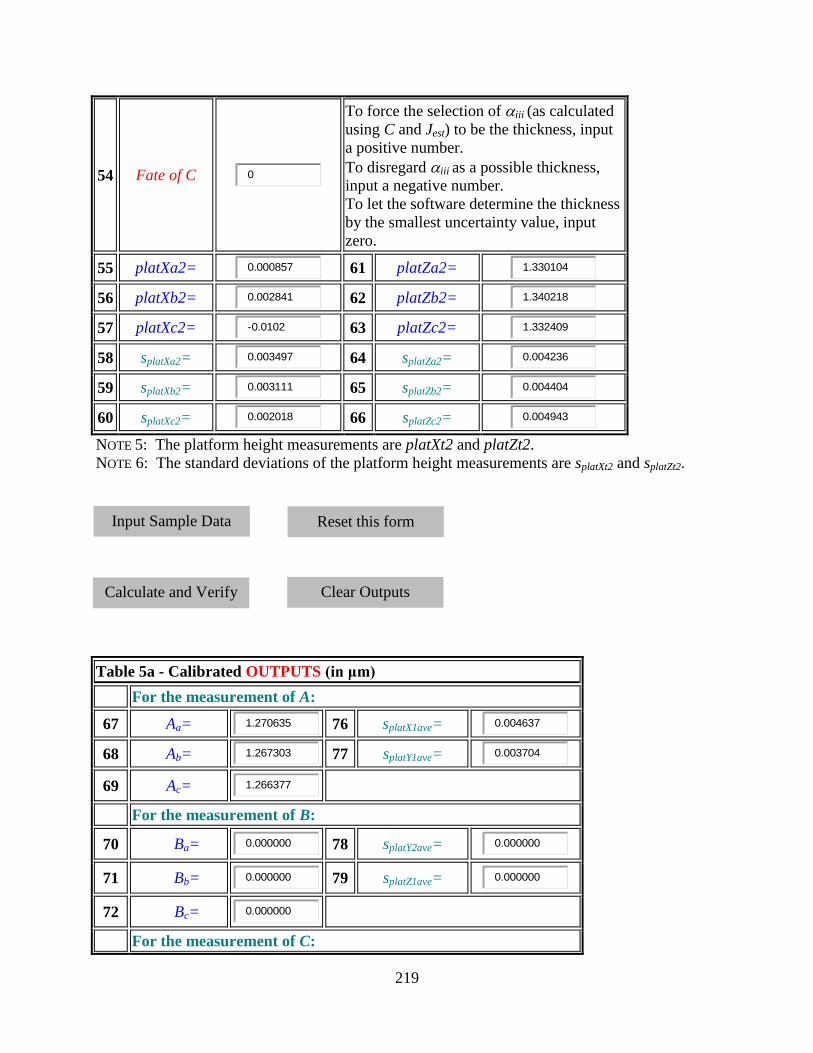
219

54 Fate of C 0

To force the selection of iii (as calculated

using C and Jest) to be the thickness, input

a positive number.

To disregard iii as a possible thickness,




zero.

55 platXa2= 0.000857 61 platZa2= 1.330104

56 platXb2= 0.002841 62 platZb2= 1.340218

57 platXc2= -0.0102 63 platZc2= 1.332409

58 splatXa2= 0.003497 64 splatZa2= 0.004236

59 splatXb2= 0.003111 65 splatZb2= 0.004404

60 splatXc2= 0.002018 66 splatZc2= 0.004943

NOTE 5: The platform height measurements are platXt2 and platZt2.

NOTE 6: The standard deviations of the platform height measurements are splatXt2 and splatZt2.

Table 5a - Calibrated OUTPUTS (in μm)

For the measurement of A:

67 Aa= 1.270635 76 splatX1ave= 0.004637

68 Ab= 1.267303 77 splatY1ave= 0.003704

69 Ac= 1.266377

For the measurement of B:

70 Ba= 0.000000 78 splatY2ave= 0.000000

71 Bb= 0.000000 79 splatZ1ave= 0.000000

72 Bc= 0.000000

For the measurement of C:

Input Sample Data


Data

Reset this form

Clear Outputs

220

73 Ca= 1.341051 80 splatX2ave= 0.002901

74 Cb= 1.349253 81 splatZ2ave= 0.004568

75 Cc= 1.354531

NOTE 7: At = (platYt1platXt1) calzA

NOTE 8: Bt = (platZt1platYt2) calzB

NOTE 9: Ct = (platZt2platXt2) calzC

NOTE 10: splatX1ave= calzA AVE(splatXa1, splatXb1, splatXc1)

NOTE 11: splatY1ave= calzA AVE(splatYa1, splatYb1, splatYc1)

NOTE 12: splatY2ave= calzB AVE(splatYa2, splatYb2, splatYc2)

NOTE 13: splatZ1ave= calzB AVE(splatZa1, splatZb1, splatZc1)

NOTE 14: splatZ2ave= calzC AVE(splatZa2, splatZb2, splatZc2)

NOTE 15: splatX2ave= calzC AVE(splatXa2, splatXb2, splatXc2)

Table 5b - Calibrated OUTPUTS (in μm)

N uLstepN uWstepN ucertN ucalN urepeat(shs)N udriftN ulinearN urepeat(samp)N ucSHN

82 A = 1.268

0.004

0.002

0.003

0.068

0.112

0.000

0.007

0.093

0.161

83 B = 0.000

0.000

0.000

NaN

NaN

NaN

NaN

0.000

0.000

NaN

84 C =1.348

0.002

0.006

0.003

0.072

0.119

0.000

0.007

0.099

0.171

NOTE 16: N = AVE (Na, Nb, Nc)

NOTE 17: uLstepA =SQRT[splatX1ave2(calzA sroughX)

2+splatY1ave

2(calzA sroughY)

2]

NOTE 18: uLstepB =SQRT[splatY2ave2(calzB sroughY)

2+splatZ1ave

2(calzB sroughZ)

2]

NOTE 19: uLstepC =SQRT[splatZ2ave2(calzC sroughZ)

2+splatX2ave

2(calzC sroughX)

2]

NOTE 20: uWstepN =σWstepN = STDEV(Na, Nb, Nc)

NOTE 21: ucertN = |σcertN N / certN|

NOTE 22: ucalN = |σ6aveN N / ̅6aveN|

NOTE 23: urepeat(shs)N = |σ6sameN N / ̅6sameN|

NOTE 24: udriftN = |(zdriftN calzN) N / [2(1.732) certN]|

NOTE 25: ulinearN = |zlinN N / (1.732)|

NOTE 26: urepeat(samp)N = σrepeat(samp)N |N|

NOTE 27: ucSHN = SQRT(uLstepN2+uWstepN

2+ucertN

2+ucalN

2+urepeat(shs)N

2+udriftN

2

+ulinearN2+ urepeat(samp)N

2)

(Each of the uncertainty components is obtained using a Type B analysis, except for

uWstepN, ucalN, urepeat(shs)N, and urepeat(samp)N which use a Type A analysis.)

Table 5c - Calibrated OUTPUTS (in μm)

85 Ccalc = 1.2681 ucCcalc = NaN

86 J = 0.0000 ucJ = NaN

221

87 i = 1.2681 uci = 0.1615

88 ii = 1.2681 ucii = NaN

89 iii = 1.3483 uciii = 0.1718

90 = 1.3483 uc = 0.1718

NOTE 28: Ccalc = A + B and ucCcalc = SQRT(ucSHA2 + ucSHB

2)

NOTE 29: J = B H and ucJ = SQRT(ucSHB2 + ucH

2) where ucH = ΔH / 6

NOTE 30: i = A + H and uci = SQRT(ucSHA2 + ucH

2)

NOTE 31: ii = Ccalc Jest and ucii = SQRT(ucCcalc2 + ucJest

2)

NOTE 32: iii = C Jest and uciii = SQRT(ucSHC2 + ucJest

2)

NOTE 33: Where ucH and ucJest are Type B components.

NOTE 34: The thickness of the suspended layer, , is the value specified for i, ii, or iii,

whichever has the smallest combined standard uncertainty value, unless Fate of

A, Fate of B, and/or Fate of C was predetermined in Tables 2, 3, and/or 4.

U = 2uc = 0.3437


3uc = 0.5155

μm

U = 1.0046

μm (a lower bound for )

+ U = 1.6919

μm (an upper bound for )



uncertainty uc, the thickness is believed to lie in the interval uc (expansion factor k=1)

representing a level of confidence of approximately 68 %.


then recalculate:

1. ok Please fill out the Preliminary Inputs Table for the measurements of A, B, and/or C and

specify Fate of A, Fate of B, and Fate of C in Tables 2, 3, and 4.

2. ok The values for tempN should be between 19.4 °C and 21.6 °C, inclusive.

3. ok The values for relative humidityN (if known) should be between 0 % and 60 %, inclusive.

4. ok The value for the design length should be greater than 0 μm and less than or equal to

1000 μm.

5. ok Are the magnifications appropriately greater than 2.5×?

6a. ok Alignment has not been ensured for the measurement of A.

6b. ok Alignment has not been ensured for the measurement of B.

6c. ok Alignment has not been ensured for the measurement of C.

222

7a. ok Data has not been leveled for the measurement of A.

7b. ok Data has not been leveled for the measurement of B.

7c. ok Data has not been leveled for the measurement of C.

8. ok The values for certN should be between 0.000 μm and 15.000 μm.

9. ok The values for σcertN should be between 0.000 μm and 0.100 μm.

10. ok The values for σ6aveN and σ6sameN should be between 0.000 μm and 0.200 μm, inclusive.

11. ok The values for ̅6aveN and ̅6sameN should be between (certN0.150 μm)/calzN and (certN

+ 0.150 μm)/calzN and not equal to 0.0 μm.

12. ok The values for zdriftN should be between 0.000 μm and 0.100 μm, inclusive.

13. ok The values for calzN should be between 0.900 and 1.100, but not equal to 1.000.

14. ok The values for zlinN should be between 0.0 % and 5.0 %, inclusive.

15. ok The values for σrepeat(samp)N should be between 0.0 % and 10.0 %, inclusive.

16. ok

The values for H and ΔH should be greater than or equal to 0.0 μm and less than 0.50 μm

if Fate of A in Table 2 is greater than or equal to zero. The values for Jest, and ucJest

should be greater than or equal to 0.0 μm and less than 0.50 μm if Fate of B or Fate of C

in Tables 3 and 4, respectively, is greater than or equal to zero.

17. ok

The values for sroughX, sroughY, and sroughZ should be greater than 0.0 μm and less than or

equal to the smallest measured value for splatXt1, splatXt2, splatYt1, splatYt2, splatZt1, and splatZt2,

respectively.

18. ok Only one of the three values for Fate of A, Fate of B, and Fate of C can be positive.

19. ok All three values for Fate of A, Fate of B, and Fate of C cannot be less than zero.

20. ok The platform heights have not been provided.

21. ok More platform heights are required for standard deviation calculations.

22. ok The platform heights (platXt1, platXt2, platYt1, platYt2, platZt1, and platZt2) should be

between 2.500 μm and 2.500 μm.

23. ok More platform standard deviations are needed.

24. ok The values for splatXt1, splatXt2, splatYt1, splatYt2, splatZt1,and splatZt2 should be between 0.00 μm

and 0.050 μm, inclusive.

25. ok The values for N should be between 2.500 μm and 2.500 μm.

26. ok The values for uLstepN and uWstepN should be less than 0.100 μm.

27. ok The value for J should be greater than or equal to 0.0 μm. If not, most likely the value

for H is too large.

28. ok The value for should be between A and C, inclusive.

223








http://www.doc.gov/





224

Appendix 8 – Overview of Propagation of Uncertainty Technique

The propagation of uncertainty technique [21-23] is used to obtain combined standard uncertainty values. Using this technique,

the combined standard uncertainty (which we are equating here with the standard deviation) for a function, f, consisting of

uncorrelated input parameters, can be calculated using the following equation:

N

i

x

i

ycy ix

fu

1

2

2

, (A8-1)

where y = f(x1, x2,…, xN).

In the special case of uncorrelated input parameters x and y in an additive relationship, as in:

byaxz , (A8-2)

where a and b are constants, Eq. (A8-1) can be rewritten as follows:

.)()( 22

yxz ba

(A8-3)

In the special case of uncorrelated input parameters x and y in a multiplicative relationship, as in:

mn yaxz , (A8-4)

where a, n, and m are constants, Eq. (A8-1) can be rewritten as follows:

2

2

2

2

2

ym

xn

z

yxz

. (A8-5)

User's Guide for RM 8096 and 8097: The MEMS 5-in-1 ... - NIST

Documents

Transcript of User's Guide for RM 8096 and 8097: The MEMS 5-in-1 ... - NIST