UserGuide - Thermo Fisher Scientific
78
UserGuide For Research Use Only. Not for use in diagnostic procedures. OncoScan TM Console 1.3 P/N 703195 Rev. 4
Transcript of UserGuide - Thermo Fisher Scientific

UserGuide
For Research Use Only.
Not for use in diagnostic procedures.
OncoScanTM Console 1.3
P/N 703195 Rev. 4

2
TrademarksAffymetrix®, OncoScan™ ,GeneChip®, NetAffx®, Command Console®, Powered by Affymetrix™, GeneChip-compatible™, Genotyping Console™, DMET™, GeneTitan®, Axiom®, CytoScan®, and GeneAtlas® are trademarks or registered trademarks of Affymetrix, Inc. All other trademarks are the property of their respective owners.
All other trademarks are the property of their respective owners.
Limited LicenseAffymetrix hereby grants to buyer a non-exclusive, non-transferable, non-sublicensable license to Affymetrix' Core Product IP to use the product(s), but only in accordance with the product labels, inserts, manuals and written instructions provided by Affymetrix. "Core Product IP" is the intellectual property owned or controlled by Affymetrix as of the shipment date of a product that covers one or more features of the product that are applicable in all applications of the product that are in accordance with the product labels, inserts, manuals and written instructions provided by Affymetrix. The license granted herein to buyer to the Core Product IP expressly excludes any use that: (i) is not in accordance with the product labels, inserts, manuals and written instructions provided by Affymetrix, (ii) requires a license to intellectual property that covers one or more features of a product that are only applicable within particular fields of use or specific applications, (iii) involves reverse engineering, disassembly, or unauthorized analysis of the product and/or its methods of use, or (iv) involves the re-use of a consumable product. Buyer understands and agrees that except as expressly set forth, no right or license to any patent or other intellectual property owned or controlled by Affymetrix is granted upon purchase of any product, whether by implication, estoppel or otherwise. In particular, no right or license is conveyed or implied to use any product provided hereunder in combination with a product or service not provided, licensed or specifically recommended by Affymetrix for such use. Furthermore, buyer understands and agrees that buyer is solely responsible for determining whether buyer possesses all intellectual property rights that may be necessary for buyer's specific use of the product, including any rights from third parties.
PatentsArrays: Products may be covered by one or more of the following patents and/or sold under license from Oxford Gene Technology: U.S. Patent Nos. 5,445,934; 5,700,637; 5,744,305; 5,945,334; 6,054,270; 6,140,044; 6,261,776; 6,291,183; 6,346,413; 6,399,365; 6,420,169; 6,551,817; 6,610,482; 6,733,977; and EP 619 321; 373 203 and other U.S. or foreign patents.
Copyright© 2015 Affymetrix Inc. All rights reserved.
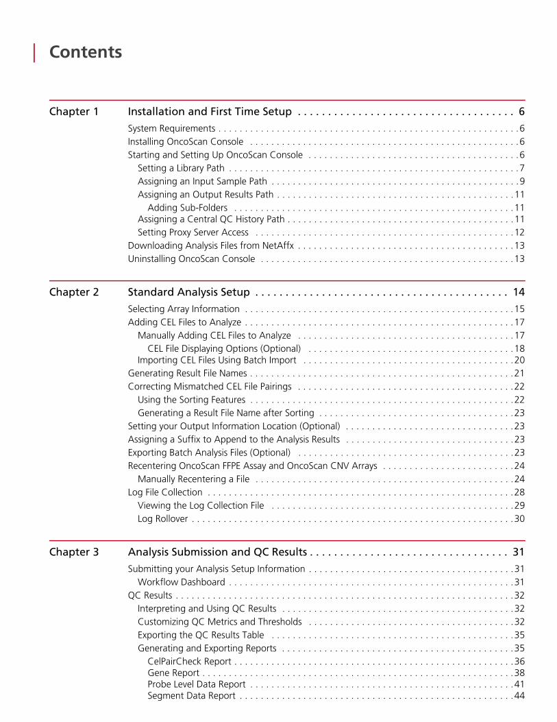
Contents
Chapter 1 Installation and First Time Setup . . . . . . . . . . . . . . . . . . . . . . . . . . . . . . . . . . . . 6
System Requirements . . . . . . . . . . . . . . . . . . . . . . . . . . . . . . . . . . . . . . . . . . . . . . . . . . . . . . . . .6Installing OncoScan Console . . . . . . . . . . . . . . . . . . . . . . . . . . . . . . . . . . . . . . . . . . . . . . . . . . .6Starting and Setting Up OncoScan Console . . . . . . . . . . . . . . . . . . . . . . . . . . . . . . . . . . . . . . . .6
Setting a Library Path . . . . . . . . . . . . . . . . . . . . . . . . . . . . . . . . . . . . . . . . . . . . . . . . . . . . . . .7Assigning an Input Sample Path . . . . . . . . . . . . . . . . . . . . . . . . . . . . . . . . . . . . . . . . . . . . . . .9Assigning an Output Results Path . . . . . . . . . . . . . . . . . . . . . . . . . . . . . . . . . . . . . . . . . . . . .11
Adding Sub-Folders . . . . . . . . . . . . . . . . . . . . . . . . . . . . . . . . . . . . . . . . . . . . . . . . . . . . .11Assigning a Central QC History Path . . . . . . . . . . . . . . . . . . . . . . . . . . . . . . . . . . . . . . . . . . .11Setting Proxy Server Access . . . . . . . . . . . . . . . . . . . . . . . . . . . . . . . . . . . . . . . . . . . . . . . . .12
Downloading Analysis Files from NetAffx . . . . . . . . . . . . . . . . . . . . . . . . . . . . . . . . . . . . . . . . .13Uninstalling OncoScan Console . . . . . . . . . . . . . . . . . . . . . . . . . . . . . . . . . . . . . . . . . . . . . . . .13
Chapter 2 Standard Analysis Setup . . . . . . . . . . . . . . . . . . . . . . . . . . . . . . . . . . . . . . . . . . 14
Selecting Array Information . . . . . . . . . . . . . . . . . . . . . . . . . . . . . . . . . . . . . . . . . . . . . . . . . . .15Adding CEL Files to Analyze . . . . . . . . . . . . . . . . . . . . . . . . . . . . . . . . . . . . . . . . . . . . . . . . . . .17
Manually Adding CEL Files to Analyze . . . . . . . . . . . . . . . . . . . . . . . . . . . . . . . . . . . . . . . . .17CEL File Displaying Options (Optional) . . . . . . . . . . . . . . . . . . . . . . . . . . . . . . . . . . . . . . .18
Importing CEL Files Using Batch Import . . . . . . . . . . . . . . . . . . . . . . . . . . . . . . . . . . . . . . . .20Generating Result File Names . . . . . . . . . . . . . . . . . . . . . . . . . . . . . . . . . . . . . . . . . . . . . . . . . .21Correcting Mismatched CEL File Pairings . . . . . . . . . . . . . . . . . . . . . . . . . . . . . . . . . . . . . . . . .22
Using the Sorting Features . . . . . . . . . . . . . . . . . . . . . . . . . . . . . . . . . . . . . . . . . . . . . . . . . .22Generating a Result File Name after Sorting . . . . . . . . . . . . . . . . . . . . . . . . . . . . . . . . . . . . .23
Setting your Output Information Location (Optional) . . . . . . . . . . . . . . . . . . . . . . . . . . . . . . . .23Assigning a Suffix to Append to the Analysis Results . . . . . . . . . . . . . . . . . . . . . . . . . . . . . . . .23Exporting Batch Analysis Files (Optional) . . . . . . . . . . . . . . . . . . . . . . . . . . . . . . . . . . . . . . . . .23Recentering OncoScan FFPE Assay and OncoScan CNV Arrays . . . . . . . . . . . . . . . . . . . . . . . . .24
Manually Recentering a File . . . . . . . . . . . . . . . . . . . . . . . . . . . . . . . . . . . . . . . . . . . . . . . . .24Log File Collection . . . . . . . . . . . . . . . . . . . . . . . . . . . . . . . . . . . . . . . . . . . . . . . . . . . . . . . . . .28
Viewing the Log Collection File . . . . . . . . . . . . . . . . . . . . . . . . . . . . . . . . . . . . . . . . . . . . . .29Log Rollover . . . . . . . . . . . . . . . . . . . . . . . . . . . . . . . . . . . . . . . . . . . . . . . . . . . . . . . . . . . . .30
Chapter 3 Analysis Submission and QC Results . . . . . . . . . . . . . . . . . . . . . . . . . . . . . . . . . 31
Submitting your Analysis Setup Information . . . . . . . . . . . . . . . . . . . . . . . . . . . . . . . . . . . . . . .31Workflow Dashboard . . . . . . . . . . . . . . . . . . . . . . . . . . . . . . . . . . . . . . . . . . . . . . . . . . . . . .31
QC Results . . . . . . . . . . . . . . . . . . . . . . . . . . . . . . . . . . . . . . . . . . . . . . . . . . . . . . . . . . . . . . . .32Interpreting and Using QC Results . . . . . . . . . . . . . . . . . . . . . . . . . . . . . . . . . . . . . . . . . . . .32Customizing QC Metrics and Thresholds . . . . . . . . . . . . . . . . . . . . . . . . . . . . . . . . . . . . . . .32Exporting the QC Results Table . . . . . . . . . . . . . . . . . . . . . . . . . . . . . . . . . . . . . . . . . . . . . .35Generating and Exporting Reports . . . . . . . . . . . . . . . . . . . . . . . . . . . . . . . . . . . . . . . . . . . .35
CelPairCheck Report . . . . . . . . . . . . . . . . . . . . . . . . . . . . . . . . . . . . . . . . . . . . . . . . . . . . .36Gene Report . . . . . . . . . . . . . . . . . . . . . . . . . . . . . . . . . . . . . . . . . . . . . . . . . . . . . . . . . . .38Probe Level Data Report . . . . . . . . . . . . . . . . . . . . . . . . . . . . . . . . . . . . . . . . . . . . . . . . . .41Segment Data Report . . . . . . . . . . . . . . . . . . . . . . . . . . . . . . . . . . . . . . . . . . . . . . . . . . . .44

Contents 4
Somatic Mutation Data Report . . . . . . . . . . . . . . . . . . . . . . . . . . . . . . . . . . . . . . . . . . . . .47Export All Data . . . . . . . . . . . . . . . . . . . . . . . . . . . . . . . . . . . . . . . . . . . . . . . . . . . . . . . . .51
Chapter 4 Matched Normal Analysis Setup . . . . . . . . . . . . . . . . . . . . . . . . . . . . . . . . . . . . 53
Selecting Array Information . . . . . . . . . . . . . . . . . . . . . . . . . . . . . . . . . . . . . . . . . . . . . . . . . . .54Adding CEL Files to Analyze . . . . . . . . . . . . . . . . . . . . . . . . . . . . . . . . . . . . . . . . . . . . . . . . . . .55
Manually Adding CEL Files to Analyze . . . . . . . . . . . . . . . . . . . . . . . . . . . . . . . . . . . . . . . . .55CEL File Displaying Options (Optional) . . . . . . . . . . . . . . . . . . . . . . . . . . . . . . . . . . . . . . .57
Importing CEL Files Using Batch Import . . . . . . . . . . . . . . . . . . . . . . . . . . . . . . . . . . . . . . . .58Generating Result File Names . . . . . . . . . . . . . . . . . . . . . . . . . . . . . . . . . . . . . . . . . . . . . . . . . .59Correcting Mismatched CEL File Pairings . . . . . . . . . . . . . . . . . . . . . . . . . . . . . . . . . . . . . . . . .60
Using the Sorting Features . . . . . . . . . . . . . . . . . . . . . . . . . . . . . . . . . . . . . . . . . . . . . . . . . .60Generating a Result File Name after Sorting . . . . . . . . . . . . . . . . . . . . . . . . . . . . . . . . . . . . . . .61Setting your Output Information Location (Optional) . . . . . . . . . . . . . . . . . . . . . . . . . . . . . . . .61Selecting a Suffix to Append to the Analysis Results . . . . . . . . . . . . . . . . . . . . . . . . . . . . . . . . .62Exporting Batch Analysis Files (Optional) . . . . . . . . . . . . . . . . . . . . . . . . . . . . . . . . . . . . . . . . .62Log File Collection . . . . . . . . . . . . . . . . . . . . . . . . . . . . . . . . . . . . . . . . . . . . . . . . . . . . . . . . . .62
Viewing the Log Collection File . . . . . . . . . . . . . . . . . . . . . . . . . . . . . . . . . . . . . . . . . . . . . .64Log Rollover . . . . . . . . . . . . . . . . . . . . . . . . . . . . . . . . . . . . . . . . . . . . . . . . . . . . . . . . . . . . .64
Appendix A Appendix A: Custom Reference Files . . . . . . . . . . . . . . . . . . . . . . . . . . . . . . . . 65
Creating your Own Reference File . . . . . . . . . . . . . . . . . . . . . . . . . . . . . . . . . . . . . . . . . . . . . .65
Appendix B Appendix B: QC Metrics - Definitions . . . . . . . . . . . . . . . . . . . . . . . . . . . . . . . . 66
Array Data QC Metrics (Overview) . . . . . . . . . . . . . . . . . . . . . . . . . . . . . . . . . . . . . . . . . . . . . .66MAPD (Median of the Absolute Values of all Pairwise Differences) . . . . . . . . . . . . . . . . . . . .66ndSNPQC (SNP Quality Control of Normal Diploid Markers) . . . . . . . . . . . . . . . . . . . . . . . . .66SNP QC Type (SNP Quality Control Type) . . . . . . . . . . . . . . . . . . . . . . . . . . . . . . . . . . . . . . .66CelPairCheck Status . . . . . . . . . . . . . . . . . . . . . . . . . . . . . . . . . . . . . . . . . . . . . . . . . . . . . . .66CelPairCheck Compare Rate . . . . . . . . . . . . . . . . . . . . . . . . . . . . . . . . . . . . . . . . . . . . . . . . .66CelPairCheck Concordance . . . . . . . . . . . . . . . . . . . . . . . . . . . . . . . . . . . . . . . . . . . . . . . . .66ndWavinessSD (Normal Diploid Waviness Standard Deviation) . . . . . . . . . . . . . . . . . . . . . . .66Y Gender Call . . . . . . . . . . . . . . . . . . . . . . . . . . . . . . . . . . . . . . . . . . . . . . . . . . . . . . . . . . .67ndCount . . . . . . . . . . . . . . . . . . . . . . . . . . . . . . . . . . . . . . . . . . . . . . . . . . . . . . . . . . . . . . .67Low Diploid Flag . . . . . . . . . . . . . . . . . . . . . . . . . . . . . . . . . . . . . . . . . . . . . . . . . . . . . . . . .67ACDC (Aberrant Cell-Derived Copy Number) . . . . . . . . . . . . . . . . . . . . . . . . . . . . . . . . . . . .67%Aberr. Cells . . . . . . . . . . . . . . . . . . . . . . . . . . . . . . . . . . . . . . . . . . . . . . . . . . . . . . . . . . .67TuScan Ploidy . . . . . . . . . . . . . . . . . . . . . . . . . . . . . . . . . . . . . . . . . . . . . . . . . . . . . . . . . . . .67Reliability Score . . . . . . . . . . . . . . . . . . . . . . . . . . . . . . . . . . . . . . . . . . . . . . . . . . . . . . . . . .68Offset Flag . . . . . . . . . . . . . . . . . . . . . . . . . . . . . . . . . . . . . . . . . . . . . . . . . . . . . . . . . . . . . .68TuScan L2R Adj . . . . . . . . . . . . . . . . . . . . . . . . . . . . . . . . . . . . . . . . . . . . . . . . . . . . . . . . . .68Adjusted Log2 Ratio . . . . . . . . . . . . . . . . . . . . . . . . . . . . . . . . . . . . . . . . . . . . . . . . . . . . . . .68Low % Aberrant Cell nGoF . . . . . . . . . . . . . . . . . . . . . . . . . . . . . . . . . . . . . . . . . . . . . . . . .68Hyb Control Intensity_AT . . . . . . . . . . . . . . . . . . . . . . . . . . . . . . . . . . . . . . . . . . . . . . . . . . .68Hyb Control Intensity_GC . . . . . . . . . . . . . . . . . . . . . . . . . . . . . . . . . . . . . . . . . . . . . . . . . . .68

Contents 5
Q3 Raw Intensity_AT . . . . . . . . . . . . . . . . . . . . . . . . . . . . . . . . . . . . . . . . . . . . . . . . . . . . . .68Q3 Raw Intensity_GC . . . . . . . . . . . . . . . . . . . . . . . . . . . . . . . . . . . . . . . . . . . . . . . . . . . . . .68AGR_AT . . . . . . . . . . . . . . . . . . . . . . . . . . . . . . . . . . . . . . . . . . . . . . . . . . . . . . . . . . . . . . . .68AGR_GC . . . . . . . . . . . . . . . . . . . . . . . . . . . . . . . . . . . . . . . . . . . . . . . . . . . . . . . . . . . . . . .69ndSNR_AT . . . . . . . . . . . . . . . . . . . . . . . . . . . . . . . . . . . . . . . . . . . . . . . . . . . . . . . . . . . . . .69ndSNR_GC . . . . . . . . . . . . . . . . . . . . . . . . . . . . . . . . . . . . . . . . . . . . . . . . . . . . . . . . . . . . . .69ndRawSNPQC . . . . . . . . . . . . . . . . . . . . . . . . . . . . . . . . . . . . . . . . . . . . . . . . . . . . . . . . . . .69Call Rate . . . . . . . . . . . . . . . . . . . . . . . . . . . . . . . . . . . . . . . . . . . . . . . . . . . . . . . . . . . . . . .69Matched Normal Compare Rate . . . . . . . . . . . . . . . . . . . . . . . . . . . . . . . . . . . . . . . . . . . . . .69Matched Normal Concordance . . . . . . . . . . . . . . . . . . . . . . . . . . . . . . . . . . . . . . . . . . . . . . .69
Array Data QC Metrics (Detailed Descriptions) . . . . . . . . . . . . . . . . . . . . . . . . . . . . . . . . . . . . .69MAPD . . . . . . . . . . . . . . . . . . . . . . . . . . . . . . . . . . . . . . . . . . . . . . . . . . . . . . . . . . . . . . . . .69
Effect of MAPD on Functional Performance . . . . . . . . . . . . . . . . . . . . . . . . . . . . . . . . . . .70ndWaviness-SD . . . . . . . . . . . . . . . . . . . . . . . . . . . . . . . . . . . . . . . . . . . . . . . . . . . . . . . . . .70ndSNPQC . . . . . . . . . . . . . . . . . . . . . . . . . . . . . . . . . . . . . . . . . . . . . . . . . . . . . . . . . . . . . . .71
Effect of ndSNPQC on Functional Performance . . . . . . . . . . . . . . . . . . . . . . . . . . . . . . . .71CelPairCheckStatus . . . . . . . . . . . . . . . . . . . . . . . . . . . . . . . . . . . . . . . . . . . . . . . . . . . . . . .73ndWavinessSD . . . . . . . . . . . . . . . . . . . . . . . . . . . . . . . . . . . . . . . . . . . . . . . . . . . . . . . . . . .74% Aberrant Cells . . . . . . . . . . . . . . . . . . . . . . . . . . . . . . . . . . . . . . . . . . . . . . . . . . . . . . . . .74Low Diploid Flag . . . . . . . . . . . . . . . . . . . . . . . . . . . . . . . . . . . . . . . . . . . . . . . . . . . . . . . . .74
Appendix C Appendix C: Algorithms . . . . . . . . . . . . . . . . . . . . . . . . . . . . . . . . . . . . . . . . . . 75
B-allele Frequencies . . . . . . . . . . . . . . . . . . . . . . . . . . . . . . . . . . . . . . . . . . . . . . . . . . . . . . . . .75LOH Algorithm . . . . . . . . . . . . . . . . . . . . . . . . . . . . . . . . . . . . . . . . . . . . . . . . . . . . . . . . . . . .75TuScan Algorithm . . . . . . . . . . . . . . . . . . . . . . . . . . . . . . . . . . . . . . . . . . . . . . . . . . . . . . . . . .75Manual Recentering Algorithm . . . . . . . . . . . . . . . . . . . . . . . . . . . . . . . . . . . . . . . . . . . . . . . .77
Appendix D Appendix D: Copy Number Effect on Somatic Mutations . . . . . . . . . . . . . . . . 78

Chapter 1
Installation and First Time Setup
System Requirements
Installing OncoScan Console1. Go to www.affymetrix.com and navigate to the following location:
Home > Products > Microarray Solutions > Instruments and Software > Software >2. Locate and download the zipped OncoScan Console software package.
3. Unzip the file, then double-click OncoScanSetup64.exe to install it.
4. Follow the directions provided by the installer.
Starting and Setting Up OncoScan Console1. Locate the OncoScan Console Desktop shortcut, then double-click on it.
The first time you launch OncoScan Console a window appears prompting you to set your Library path. (Figure 1.1)
2. Click OK.
Operating System
Windows® 7 Professional (64-bit) with Service Pack 1 installed
Figure 1.1 Library path message

Chapter 1 | Installation and First Time Setup 7
The following window appears: (Figure 1.2)
Setting a Library PathMake sure your assigned Library Path folder is placed in a high-level, easy to access, local directory. (Example: C:\)
1. Click the Library File path field’s browse button.
An Explorer window appears.
2. Navigate to a high-level, easy to access, local directory.(Example: C:\)
3. Click Create New Folder (lower left) to create a Library Files path folder.
4. In the Create New Folder field, enter a folder name. (Example: C:\OncoScanLib)
5. Click OK.
Figure 1.2 Set Library Path Explorer window
NOTE: During the installation process, outdated library files are auto-detected, then automatically moved to an archive folder. Make sure you always download the latest available library files after installing a new version of OncoScan Console.

Chapter 1 | Installation and First Time Setup 8
The following window and message appears. (Figure 1.3)
6. Acknowledge the message, then click OK.
To download files from NetAffx, go to Downloading Analysis Files from NetAffx on page 13.
The following message appears. (Figure 1.4).
7. Acknowledge the message, then click OK.
8. Click the Utility Actions button, then click on Configuration.
Figure 1.3 Library Files message
Figure 1.4 Library path message

Chapter 1 | Installation and First Time Setup 9
The Configuration window tab appears, as shown in Figure 1.5.
Assigning an Input Sample PathThe Input Sample Path folder is the location you normally store your CEL files.
1. Click Add.
NOTE: You only need to perform the following steps once, as the data and selections you enter (throughout this section) are retained for your convenience.
Figure 1.5 Main window

Chapter 1 | Installation and First Time Setup 10
The following window appears: (Figure 1.6)
2. Navigate to the recommended C:\Users directory, then click the Create New folder. (Figure 1.6)
3. In the Create New Folder window field, enter a folder name. (Example: C:\Users\YourName\OncoScan_CEL_files), then click OK. (Figure 1.7)
4. Click OK to close the window.
Your new input folder and its path appear, as shown in Figure 1.8.
Figure 1.6 Add Input sample files window
Figure 1.7 Add Input sample files window

Chapter 1 | Installation and First Time Setup 11
Assigning an Output Results Path1. Click the Output results path field’s browse button.
An Explorer window appears.
2. Navigate to the recommended C:\Users directory, then click Create New Folder.
3. In the Create New Folder field, enter a folder name. (Example: C:\Users\YourName\OncoScan_results_files)
4. Click OK.
Your new output folder and its path appear, as shown in Figure 1.8.
Adding Sub-Folders
1. The Output results path field’s browse button to return to your newly assigned output folder.
2. Click Create New Folder.
3. Enter a sub-folder name.
4. Click OK.
The newly created sub-folders now appear in the output result information window.
5. Repeat the above steps 1-4 to add more sub-folders.
Assigning a Central QC History Path1. Click the Central QC history path field’s browse button.
An Explorer window appears.
2. Navigate to: C:\ProgramData\Affymetrix\OncoScan
3. Click Create New Folder (lower left) to create a Central QC history path folder.
4. In the Create New Folder field, enter a folder name. (Example: My_QC_History)
5. Click OK, then click OK again.
Your QC History folder now appears in the Central QC History path field, as shown in Figure 1.8.
TIP: Add sub-folders to your newly assigned output result path’s folder to better organize your output results,

Chapter 1 | Installation and First Time Setup 12
Setting Proxy Server AccessThis configuration should only be done if the user’s system has to pass through a proxy server to access Affymetrix NetAffx server.
In most cases, when a customer requires the use of a proxy, they can set a system-level proxy using their default Internet browser while keeping the OncoScan Console default setting at Use System Proxy.
1. From the Configuration window tab, click .
Figure 1.8 Main window showing assigned paths
NOTE: You may need to contact your IT Department for system proxy information.

Chapter 1 | Installation and First Time Setup 13
The Custom Proxy Server Settings window opens (Figure 1.9).
2. Click the Enable Custom Proxy Server checkbox, then complete the required fields.
3. Click Save.
4. Click Save to save all your Configuration window tab settings and paths.
Downloading Analysis Files from NetAffxAfter your Library Path folder is created, you must download the library files that OncoScan Console uses to analyze and annotate the data from NetAffx.
1. Click on Utility Actions -> Download Library Files or open your Internet browser and go to www.affymetrix.com.
2. Enter your NetAffx user name and password or click Register Now to create a NetAffx account.
The Choose Files window opens with a list of array types supported by the software.
3. Click the OncoScan array checkbox.
4. Click Next.
The Download Progress window displays the progress of the downloading and unpacking of the files.
Uninstalling OncoScan Console1. From the Windows Start Menu, navigate to the Windows Control Panel.
2. Navigate to the Uninstall or change a program.
3. Locate the OncoScan Console application, then perform the uninstall as you normally would.
Figure 1.9 Configuration window
NOTE: This proxy user ID and password is NOT the same ID and password used to connect to the Affymetrix NetAffx server.
NOTE: You can also download the analysis library file package from directly from www.affymetrix.com. After downloading, unzip the contents of the file directly into the Library folder you assigned earlier.
If you go to the website (outside of OncoScan Console) to download the analysis library file package, you must close, then restart OncoScan Console in order for it to recognize the newly downloaded files.
NOTE: Your data and library files are NOT deleted by uninstalling OncoScan Console.
Chapter 2
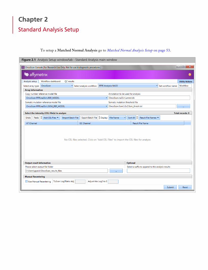
Standard Analysis Setup
To setup a Matched Normal Analysis go to Matched Normal Analysis Setup on page 53.
Figure 2.1 Analysis Setup window/tab - Standard Analysis main window

Chapter 2 | Standard Analysis Setup 15
Selecting Array Information
1. From the Select array type drop-down list, click to select either OncoScan or OncoScan_CNV.
As long as your library file folder contains the necessary analysis files for the array, your configuration paths are established and your Array Information fields auto-populate, as shown in Figure 2.2.
Somatic mutation file selection is NOT available with the OncoScan_CNV array type, as shown in Figure 2.3.
2. From the Select analysis workflow drop-down list, click to select an analysis workflow.
FFPE Analysis: NA33 - Use this workflow for analyzing FFPE samples.
Non-FFPE Analysis: NA33 - Use this workflow for analyzing Non-FFPE samples.
Control Analysis: NA33 - Use this workflow for analyzing the Ref103 control sample.
FFPE Analysis including Matched Normal: NA33 - Use this workflow when you have DNA from normal and tumor tissue from the same FFPE fixed specimen. To setup a Matched Normal Analysis go to page 53.
Reference Generation: NA33 - Select this option when you want to create your own Reference File. See Appendix A: Custom Reference Files on page 65.
3. (Optional) Enter a Workflow name. By default, the Set workflow name is Workflow. Click (upper right) to enter a different workflow name.
Figure 2.2 Standard Analysis Configuration - OncoScan array
Figure 2.3 Standard Analysis Configuration - OncoScan_CNV array
NOTE: The Select array type drop-down list includes only the array types from the library(analysis) files that have been downloaded from NetAffx or copied from the Librarypackage provided in the OncoScan installation package.
IMPORTANT: After adding new library files to the library file folder, always close and re-launch OncoScan Console to ensure the newly added files are recognized by the software.
TIP: Customizing a Workflow name can be a useful tool in keeping track of analysis workflows as all the related output files (outside of the OSCHP file) begin with this workflow name.

Chapter 2 | Standard Analysis Setup 16
4. Select a Copy Number reference model file. By default, it is set to the most recently used reference model file. If you created your own reference model file, click the drop-down list to select your .REF_MODEL. Check to ensure the reference model file is appropriate for the sample type.
The Annotation file is automatically selected for you and is based on your selected reference model file. (Example: OncoScan.na33.v1.annot.db)
5. Select a Somatic mutation reference model file. (OncoScan array only. Not applicable to OncoScan_CNV array.)
By default, it is set to the most recently used SOM reference model file. If you created your own reference model file, click the drop-down list to select your .SOM_REF_MODEL.
6. Check to ensure the somatic mutation reference model file is appropriate for the sample type. If you need to change it, click the Browse button, navigate to the appropriate threshold .txt file, then click OK.
NOTE: The Annotation to be used for analysis field is auto-populated based on your RefModel file selection. The analysis is not be permitted to run if the appropriate annotationfile is not available in your Library folder.
IMPORTANT: If the Reference Model File and Somatic mutation Reference Model Filewere created independently of each other, a warning message appears after you clickSubmit (to start the Workflow Analysis process). Click OK to acknowledge the message.

Chapter 2 | Standard Analysis Setup 17
Adding CEL Files to AnalyzeYou can manually add CEL files or import them as a tab-delimited text file.
Manually Adding CEL Files to AnalyzeTo add a batch file containing the list of CEL files, see Importing CEL Files Using Batch Import on page 20.
1. From the Select the intensity (CEL) file(s) to analyze pane, click the Add CEL files drop-down.
2. Click AT Channel.
The CEL file window appears. ( (Figure 2.4)).
3. Click any header to sort your files or click the Files of type drop-down to filter your CEL files by AT Channel, as shown in Figure 2.5.
4. Single click, Ctrl click, or Shift click (to select multiple AT Channel files)
Figure 2.4 CEL file folder -Example
IMPORTANT: Affymetrix recommends using an “A” or “C” as the last character todesignate the channel in the CEL file naming convention. Example: “_AS_05A.CEL” is anAT Channel file, while “_AS_05C.CEL” is a GC Channel file. See Figure 2.4.
Figure 2.5 Files of type drop-down list

Chapter 2 | Standard Analysis Setup 18
5. Click Open.
The AT Channel fields are now populated. (Figure 2.6)
6. Click the Add CEL files drop-down.
7. Click GC Channel. The CEL file window appears. (Figure 2.4)
8. Click any header to sort your files or click the Files of type drop-down to filter your CEL files by GC Channel, as shown in Figure 2.7.
9. Single click, Ctrl click, or Shift click (to select multiple GC Channel files).
10. Click Open.
The GC Channel fields are now populated. (Figure 2.8)
CEL File Displaying Options (Optional)The File Name drop-down list (Figure 2.9) is dynamically populated and based on what attributes are populated in the ARR file.
To use this display option, you must:
1. Provide the appropriate attributes at the time of sample registration in AGCC.
Figure 2.6 AT Channel file list
Figure 2.7 Files of type drop-down list
Figure 2.8 CEL Files Loaded to Analyze
Chapter 2 | Standard Analysis Setup 19
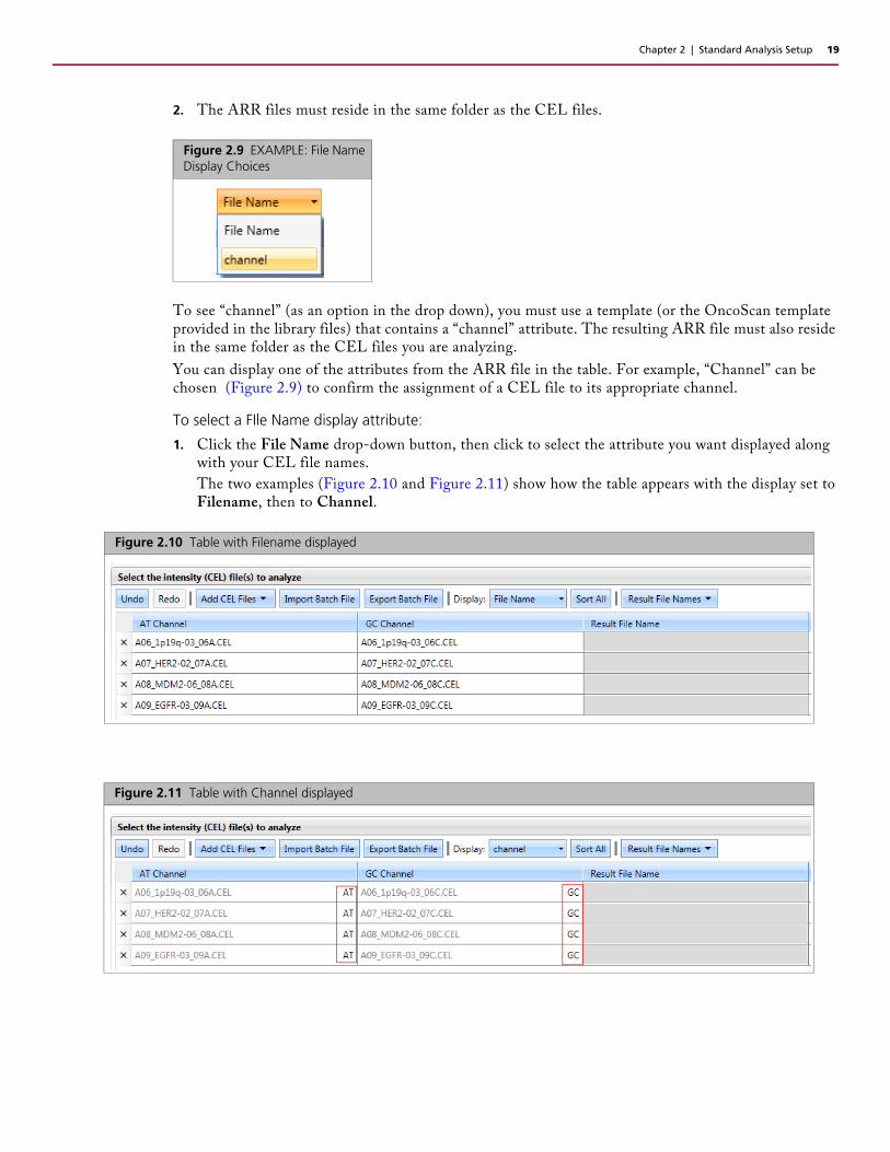
2. The ARR files must reside in the same folder as the CEL files.
To see “channel” (as an option in the drop down), you must use a template (or the OncoScan template provided in the library files) that contains a “channel” attribute. The resulting ARR file must also reside in the same folder as the CEL files you are analyzing.
You can display one of the attributes from the ARR file in the table. For example, “Channel” can be chosen (Figure 2.9) to confirm the assignment of a CEL file to its appropriate channel.
To select a FIle Name display attribute:
1. Click the File Name drop-down button, then click to select the attribute you want displayed along with your CEL file names.
The two examples (Figure 2.10 and Figure 2.11) show how the table appears with the display set to Filename, then to Channel.
Figure 2.9 EXAMPLE: File Name Display Choices
Figure 2.10 Table with Filename displayed
Figure 2.11 Table with Channel displayed

Chapter 2 | Standard Analysis Setup 20
Importing CEL Files Using Batch ImportOncoScan Console allows import of CEL files using a batch file. The batch file must be saved as a text (Tab-delimited) format and include the full directory path for your CEL files (as shown in Figure 2.12).
The format for this tab-delimited file is 3 columns (A,B, and C) with the headers:
ATCHANNELCEL
GCCHANNELCEL
RESULT
You must provide the full path to the CEL files for each Channel column. (Example: C:\Desktop\OncoScan\Data\Sample1.cel)
1. Click Import Batch File
A File window appears.
2. Navigate to your text (tab-delimited) file location, then click on the file you want to import.
3. Click Open.
The AT, GC, and Result File Name fields are now populated. (Figure 2.13)
TIP: The resulting OSCHP files are saved to your output path location, therefore it is not necessary to include a path under RESULT. Simply enter the desired results filename in this column.
Figure 2.12 List from Microsoft Excel
IMPORTANT: The Microsoft Excel application must be closed before you import (clickOpen).
Figure 2.13 Tab-delimited text file imported into OncoScan Console

Chapter 2 | Standard Analysis Setup 21
Generating Result File NamesResults File Names can either be entered in manually or OncoScan Console can generate them automatically.
To manually enter a Results File Name:
1. Single-click inside the appropriate Results Name File field to produce a cursor, then type in the file name you want.
To auto-generate a suggested Result File Name:
1. After the AT and GC Channel lists are populated, click the Result File Names drop-down, then select Auto Generate Output Name.
2. The Result File Name column is now populated with suggested filenames for each pairing. (Figure 2.14)
Common root names should be consistent all the way up to the last character of the CEL file name prior to the .cel extension. If there is a paired file mis-match, the Results File Name appears as Output1. (Figure 2.15)
If Output1 or subsequent Outputs (Output 2, Output 3...) appear, investigate the validity of your original pairing. See Correcting Mismatched CEL File Pairings on page 22.
NOTE: If you use the suffix option (Assigning a Suffix to Append to the Analysis Resultson page 23) and enter your Result File Names manually, your assigned suffix appears inthe Results File Name column.
If you auto-generate your Results File Names, your assigned suffix appears in the ResultsFile Name column, but it does get added to your final OSCHP file name(s).
NOTE: During the Result File Name auto-generation process, the file names are comparedto identify their common root name for use as a results file name. Generally, the last 5characters of each CEL file name are ignored, then the remaining root names of the ATand GC file names are compared. If the root names of the AT and GC channel match, thenthe root name is used in the Results File Name field. The one exception is if your arrayname “_(OncoScan)” is appended to the file name during registration in AffymetrixGeneChip Command Console (AGCC). In this case, the “_(OncoScan)” is ignored during thecomparison, but then added back in the Results File Name field.
Figure 2.14 Result File Name list
Figure 2.15 Result File Name “Output”

Chapter 2 | Standard Analysis Setup 22
To edit an auto-generated Result File Name:
1. Click on the Result File name you want to edit.
2. After the cursor appears, edit the filename as you normally would.
3. Click outside the row to save your edit.
To clear the entire Result File Name column:
1. Click the Result File Names drop-down button, then select Clear Column.
The column is now cleared and ready for new Result File Name entries.
Correcting Mismatched CEL File PairingsIf there is a paired file mismatch, the Results File Name appears as Output1, Output2, Output3, etc.
A paired file mismatch is most likely caused by an incorrect CEL filename pairing and not a mismatch of your native CEL files.
A simple way to correct mismatches is to sort the AT and GC columns so that files with the same root names are next to each other.
Using the Sorting Features
To sort an individual column:
1. Click on either the AT or GC Channel header.
The column is now sorted in an ascending order.
2. Click on either the AT or GC Channel header again to reverse the sorting order.
To sort both columns simultaneously:
1. Click Sort All.
The contents of each column are now sorted together in an ascending order.
2. Click Sort All again.
The contents of each column are now sorted together in a descending order.
To swap CEL files between columns:
1. Click and drag a column CEL entry onto another column CEL entry, then release the mouse button.
The CEL entries have now swapped column positions.
To reorder the CEL files in a column:
1. Click and drag a CEL file to another position within the column, then release the mouse button.
The CEL file is now at its new position.
To add a cell to a column:
1. Click and drag a column cell to the top or bottom border line of a neighboring cell, then release the mouse button.
TIP: Common root names should be consistent all the way up to the last character of the cel file name prior to the .cel extension. Affymetrix recommends using an “A” or “C” as the last character to designate the channel in the CEL file naming convention. Example: “_AS_05A.CEL” is an AT Channel file, while “_AS_05C.CEL” is a GC Channel file.

Chapter 2 | Standard Analysis Setup 23
Generating a Result File Name after Sorting1. After your AT and GC Channel lists are properly sorted, click the Result File Names drop-down,
then select Auto Generate Output Names.
The Result File Name column is now populated with suggested filenames for each pairing.
If OncoScan Console detects an inconsistency between the AT and GC file names to be paired, a Result File Name labeled, “Output n” reappears.
Repeat the sorting steps above, then try to Auto Generate Output Names again until a successful Result File Name(s) appears.
Setting your Output Information Location (Optional) The Output result information path (lower left) is retained from your initial setup.
To select a different folder to store your results:
1. Click the browse button, then navigate to the folder you want. If you want to change the default folder, see Assigning an Output Results Path on page 11.
Assigning a Suffix to Append to the Analysis ResultsYou can append a suffix at the end of all your Results File Names. This is useful when tracking versions of the analysis files used to generate the resulting OSCHP files.
To use an appending suffix:
1. Click inside the Select a suffix to append to the analysis results field to enter an appending file suffix. (Figure 2.16)
Your currently displayed Result Name Files are appended (in real-time) as you type in your suffix.
Exporting Batch Analysis Files (Optional)You can export the information shown in the AT, GC, and Results File Names fields to Microsoft Excel as a tab-delimited file for review and/or further batch editing.
1. Click Export Batch File.
A File window appears.
2. Navigate to the location where you want to save the file.
3. Make sure the Files of type is set to Tab Delimited File(s), then click Save.
IMPORTANT: Confirm that both columns are sorted in the same direction. If they are,examine the files and confirm they are paired correctly. The file names (excluding the lastcharacter before the .CEL) MUST match exactly.
Figure 2.16 Adding a suffix
NOTE: If you are saving the same OSCHP file into the same output file folder that containsyour originally run OSCHP file with an identical suffix, a “2” is automatically added to thefilename to differentiate the two runs of identical CEL file names.
NOTE: Once an analysis is submitted, a tab delimited file containing the cel file selectionsis automatically saved in your designated output folder.
Chapter 2 | Standard Analysis Setup 24
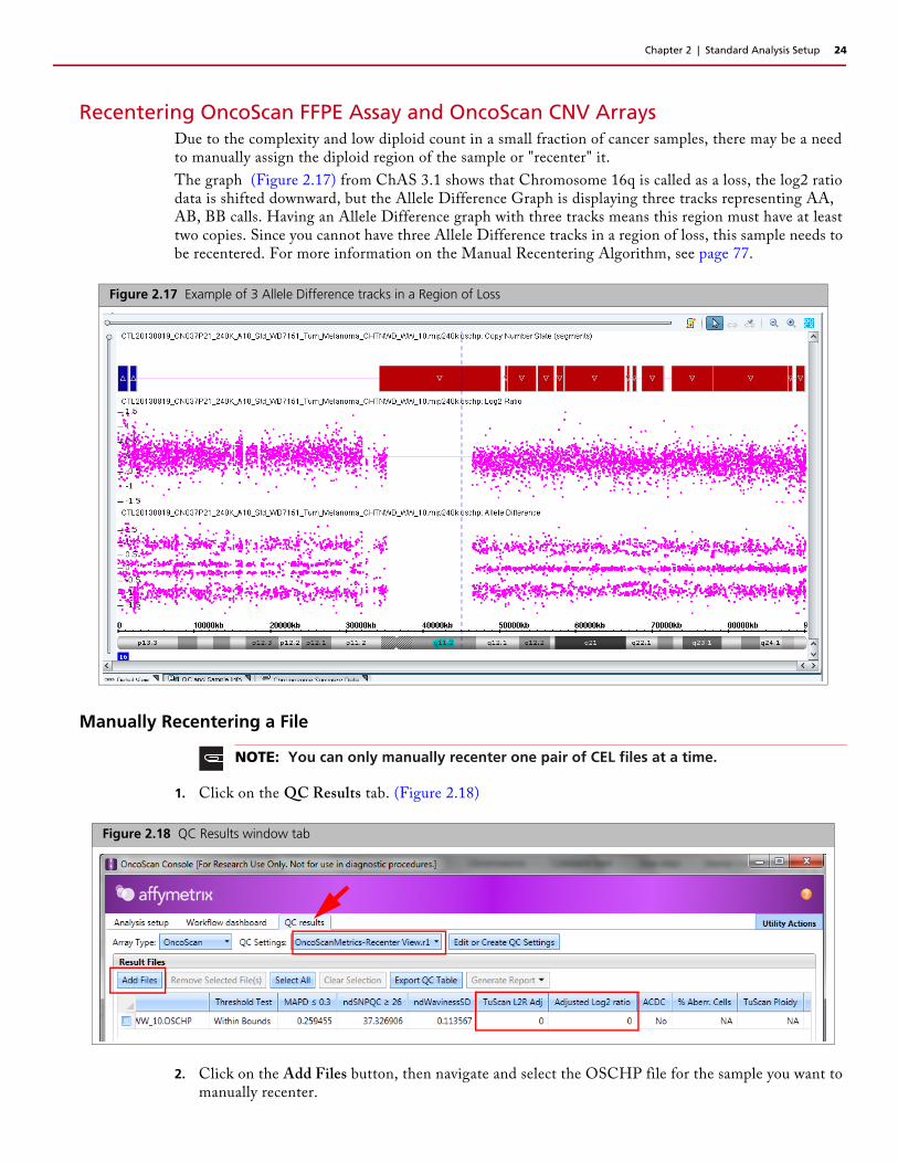
Recentering OncoScan FFPE Assay and OncoScan CNV ArraysDue to the complexity and low diploid count in a small fraction of cancer samples, there may be a need to manually assign the diploid region of the sample or "recenter" it.
The graph (Figure 2.17) from ChAS 3.1 shows that Chromosome 16q is called as a loss, the log2 ratio data is shifted downward, but the Allele Difference Graph is displaying three tracks representing AA, AB, BB calls. Having an Allele Difference graph with three tracks means this region must have at least two copies. Since you cannot have three Allele Difference tracks in a region of loss, this sample needs to be recentered. For more information on the Manual Recentering Algorithm, see page 77.
Manually Recentering a File
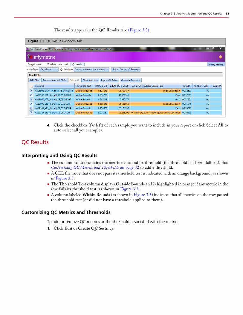
1. Click on the QC Results tab. (Figure 2.18)
2. Click on the Add Files button, then navigate and select the OSCHP file for the sample you want to manually recenter.
Figure 2.17 Example of 3 Allele Difference tracks in a Region of Loss
NOTE: You can only manually recenter one pair of CEL files at a time.
Figure 2.18 QC Results window tab

Chapter 2 | Standard Analysis Setup 25
3. From the QC Settings drop-down menu, select Recenter View r1, then make a note the file’s TuScan L2R Adj value. You will need to enter this value into the TuScan L2R Adj field in the Analysis setup window tab when reprocessing the associated pair of CEL files.
4. Click on the Analysis setup tab.
Make sure there are no CEL files present in the Select the Intensity (CEL) file(s) to analyze pane. (Figure 2.19)
5. Add the AT Channel file and its associated GC Channel file, as described in Manually Adding CEL Files to Analyze on page 17.
The paired CEL files appear, as shown in Figure 2.20.
6. Click the Use Manual Recentering check box.
7. Enter the TuScan Log2Ratio Adj value you recorded in Step 3.
Figure 2.19 Empty Select the Intensity (CEL) file(s) to analyze pane
Figure 2.20 Empty Select the Intensity (CEL) file(s) to analyze pane

Chapter 2 | Standard Analysis Setup 26
8. Enter a Adjust this Log2 to 0 value. This value is the currently-reported median log2 ratio for the region you would like to call Normal Diploid.
9. Click Submit.
10. The Workflow dashboard window tab appears and reprocessing begins.
After reprocessing has successfully completed, the QC results of the OSCHP and RC.OSCHP file appear together for comparison, as shown in Figure 2.21.
NOTE: Adjusted Log2 ratio in the Recenter View records the amount you manuallyadjusted the log2 ratios for this analysis. If you did not manually recenter this data, thisvalue will be 0.
For methods on determining the median log2 ratio for a region, see the ChAS 3.1 UserGuide (page 64) available at www.affymetrix.com.
NOTE: An RC is automatically appended onto the OSCHP file as it goes through manualrecentering process. Example: RC.OSCHP
Figure 2.21

Chapter 2 | Standard Analysis Setup 27
The graph (Figure 2.22) from ChAS 3.1, displays the original OSCHP file (pink data) and the manually recentered RC.OSCHP (green data).
By inputting both the TuScan Log2 Ratio value (derived from the algorithm) and the median Log2 Ratio value (for the region you have determined to be diploid, Chromosome 16q for our example), the Recentering Algorithm has recentered the log2 ratio data (for the region determined to be diploid) around 0 and there is no longer a loss segment called in this region.
Figure 2.22 Example original oschp file (pink data) and the manually recentered RC.OSCHP (green data)
NOTE: For details on how to view .OSCHP and RC.OSCHP files in ChAS, see the ChAS 3.1User Guide.

Chapter 2 | Standard Analysis Setup 28
Log File Collection
Do the following if you experience any issues or failures with your analysis:
1. Click the Utilities button (top right of the OncoScan Console window)
2. Click to select Log Collection.
The following window appears. (Figure 2.23)
3. Use OncoScan Console’s default location of C:\ or navigate to a folder location of your choice.
4. Click Create New Folder, then enter a folder name for your log.
5. Click OK.
Figure 2.23 Log Collection File window

Chapter 2 | Standard Analysis Setup 29
The following window appears confirming your log file has been saved as a zip file.
6. Click OK to close the window.
Viewing the Log Collection File1. Use Windows Explorer to navigate to the location.
(Example: C:\ProgramData\Affymetrix\OncoScan\log)
2. Locate the zip folder you created earlier, then double-click on it.
The folder opens.
Figure 2.24 Example: Zip file contents of a Log Collection
NOTE: The auto-generated log collection zip file contains the full contents of the folderand all QC History log files found in the configured QC History File path. By default, thezip file resides here: C:\ProgramData\Affymetrix\Oncoscan\log

Chapter 2 | Standard Analysis Setup 30
3. Extract the zipped folder’s contents, as you normally would. (Figure 2.25)
Log RolloverWhen the software determines that the log file for the Analysis Workflow (C:\ProgramData\Affymetrix\OncoScan\log\AnalysisWorkflow.log) has reached a defined size (approximately 4MB), the following steps will be completed:
A sub-folder will be created in C:\ProgramData\Affymetrix\OncoScan\log called 'Log*' (the '*' denotes the current date and time).
A zip file called RolledLogFile*.zip is created in that folder. The '*' is the same date and time used for the folder name. The files in the C:\ProgramData\Affymetrix\OncoScan\log folder and all files found in the currently selected QC History Log folder will be included in this zip file.
The Analysis Workflow files that are associated with analysis workflows that are no longer active on the Dashboard will be deleted from: C:\ProgramData\Affymetrix\OncoScan\log
A new AnalysisWorkflow.log file will be created here: C:\ProgramData\Affymetrix\OncoScan\log
Figure 2.25 Example: Zip file contents of a Log Collection

Chapter 3
Analysis Submission and QC Results
Submitting your Analysis Setup Information1. After the information in the Analysis Setup window/tab is complete, click Submit.
The Workflow dashboard tab appears and processing begins.
Workflow DashboardThe OncoScan Console Analysis Workflow Dashboard uses a progress bar to track the software’s ongoing analysis tasks, then delivers the results of analyses. (Figure 3.1)
To pause and restart a Workflow analysis in progress:
1. Click Pause to stop the Workflow that is in progress.
2. Click Resume to restart the Workflow analysis.
To abort the Workflow in progress:
1. Click Pause to stop the Workflow that is in progress.
1. Click the X (upper right corner) of the Workflow pane.
A warning message appears.
2. Click OK to acknowledge the message.
After analysis is complete, a Workflow completed successfully message appears. (Figure 3.2)
3. To view the results, click .
Figure 3.1 .CEL file analysis inside the Workflow dashboard
Figure 3.2 Workflow Dashboard example with multiple Single Samples loaded
Chapter 3 | Analysis Submission and QC Results 32
The results appear in the QC Results tab. (Figure 3.3)
4. Click the checkbox (far left) of each sample you want to include in your report or click Select All to auto-select all your samples.
QC Results
Interpreting and Using QC Results The column header contains the metric name and its threshold (if a threshold has been defined). See
Customizing QC Metrics and Thresholds on page 32 to add a threshold.
A CEL file value that does not pass its threshold test is indicated with an orange background, as shown in Figure 3.3.
The Threshold Test column displays Outside Bounds and is highlighted in orange if any metric in the row fails its threshold test, as shown in Figure 3.3.
A column labeled Within Bounds (as shown in Figure 3.3) indicates that all metrics on the row passed the threshold test (or did not have a threshold applied to them).
Customizing QC Metrics and Thresholds
To add or remove QC metrics or the threshold associated with the metric:
1. Click Edit or Create QC Settings.
Figure 3.3 QC Results window tab

Chapter 3 | Analysis Submission and QC Results 33
The following window appears: (Figure 3.4)
The existing QC Metric OncoScan.Default contains the main metrics used in determining whether the array passes or not.
OncoScan.All contains additional algorithm metrics that can be used for advanced troubleshooting.
To view the Thresholds included with OncoScan Console, see Appendix B: QC Metrics - Definitions on page 66.
Figure 3.4 Edit or create QC Results window tab
Chapter 3 | Analysis Submission and QC Results 34
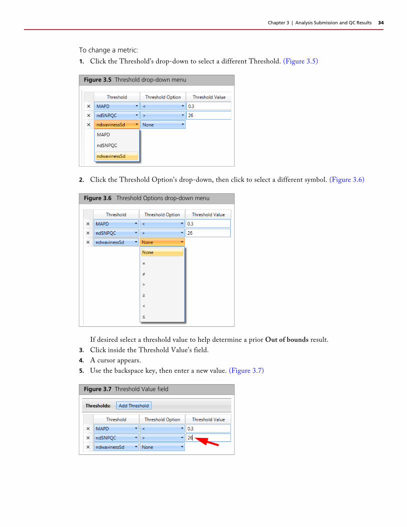
To change a metric:
1. Click the Threshold’s drop-down to select a different Threshold. (Figure 3.5)
2. Click the Threshold Option’s drop-down, then click to select a different symbol. (Figure 3.6)
If desired select a threshold value to help determine a prior Out of bounds result.
3. Click inside the Threshold Value’s field.
4. A cursor appears.
5. Use the backspace key, then enter a new value. (Figure 3.7)
Figure 3.5 Threshold drop-down menu
Figure 3.6 Threshold Options drop-down menu
Figure 3.7 Threshold Value field

Chapter 3 | Analysis Submission and QC Results 35
To add a new a QC Metric(s):
1. Click Add Threshold.
A new Threshold is added to the table.
2. Click the Threshold’s drop-down menu to select your new threshold.
A new Threshold Option is added to the new row.
3. Click the Threshold Option’s drop-down, then click to select a symbol.
A text box for Threshold Value is added to the column.
4. Click inside the Threshold Value’s field.
A cursor appears.
5. Enter a new value
6. You must enter a filename unless you are editing (and plan to overwrite) a previous QC Metric filename
7. Click Save.
Exporting the QC Results Table
To export your QC Results table:
1. Click Export QC Table to export all the data shown in the table (no checking of the checboxes is required).
A File window appears.
2. Navigate to the location you want.
3. Enter a File Name or use the default QCMetrixTable.txt.
Make sure the Files of type is set to Tab Delimited File(s).
4. Click Save.
The tab-delimited text version of the QC results table is now saved for your records. (Figure 3.8)
Generating and Exporting Reports
To Generate and Export your Results File table(s) as a tab-delimited text file:
1. Click the checkbox next to the Results File(s) you want to generate a report for, or click Select All.
2. Click to display the report menu options.
CelPairCheck Report on page 36
Gene Report on page 38
Probe Level Data Report on page 41
Segment Data Report on page 44
Somatic Mutation Data Report on page 47
Export All Data on page 51
Figure 3.8 Exported as a tab-delimited text file

Chapter 3 | Analysis Submission and QC Results 36
CelPairCheck ReportThis report is based off the signature SNPs and indicates whether the cel files selected as the AT and GC files were likely from the same sample and assigned to the correct channel.
Do the following to export a CelPairCheck Report (aka SignatureSNP Report):
1. Click Export CelPairCheck Report. (Figure 3.9)
Your previously assigned Output folder file window appears. (Figure 3.10)
If you have not yet assigned an output folder, see Assigning an Output Results Path on page 11.
2. The default root filename is Result. Click inside the File Name field to enter a different root filename, then click Save.
Figure 3.9 Generate Report drop-down menu
Figure 3.10 OncoScan Output folder window

Chapter 3 | Analysis Submission and QC Results 37
A progress bar appears while your report generates, followed by a report finished successfully message, as shown in Figure 3.11.
3. Click Yes.
The OncoScan Output folder window appears.
4. Locate the SignatureSNP Report text file, then open it in Microsoft Excel.
The following window appears. (Figure 3.12)
Figure 3.11 CelPairCheck Report successful
Figure 3.12 SignatureSNP report
Filename Name of the OSCHP file containing the data
CEL Filename Name of cel file.
Channel The Channel file from which the signal is measured. "A" is the AT CEL, "C" is the GC CEL.
CelPairCheckStatus CelPairCheck is a test that inspects each pair of intensity (*.cel) files to determine whether the files have been properly paired and assigned to the correct channel. In addition to accidental mispairing of intensity files while setting up the analysis, a tracking problem during the assay may result in a sample being assigned to the wrong GeneChip array. As a result CelPairCheck ignores file names, and instead inspects the genotypes in the two intensity files to detect file mispairings. To learn more about CelPairCheck Status, see page 73.
CelPairCheckCallRate CelPairCheckCallRate is the percentage of signature SNPs that make a genotype call for a given CEL file.
CelPairCompareRate This metric is the percentage of signature SNP control markers whose genotypes are compared between the AT and GC channels.
CelPairConcordance This metric is the concordance of a set of signature SNP genotypes compared between AT and GC CEL files. If CelPairCheck Compare Rate is high but CelPairCheck Concordance is low, then CelPairCheck Status will report "PossibleCELmispair".
SIG_001..00N Genotype for signature snp 1..n
Chapter 3 | Analysis Submission and QC Results 38
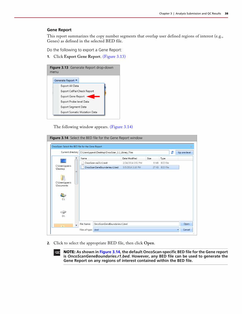
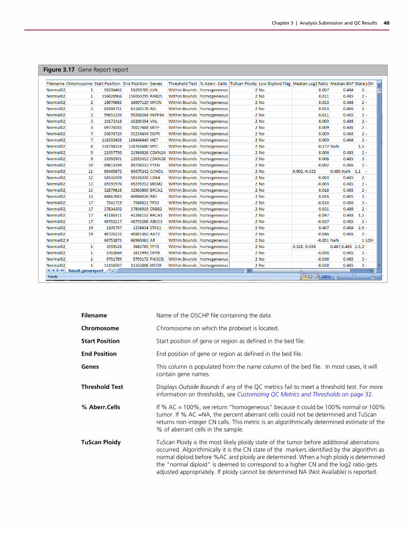
Gene ReportThis report summarizes the copy number segments that overlap user defined regions of interest (e.g., Genes) as defined in the selected BED file.
Do the following to export a Gene Report:
1. Click Export Gene Report. (Figure 3.13)
The following window appears. (Figure 3.14)
2. Click to select the appropriate BED file, then click Open.
Figure 3.13 Generate Report drop-down menu
Figure 3.14 Select the BED file for the Gene Report window
NOTE: As shown in Figure 3.14, the default OncoScan-specific BED file for the Gene reportis OncoScanGeneBoundaries.r1.bed. However, any BED file can be used to generate theGene Report on any regions of interest contained within the BED file.

Chapter 3 | Analysis Submission and QC Results 39
Your previously assigned Output folder file window appears. (Figure 3.15)
If you have not yet assigned an output folder, see Assigning an Output Results Path on page 11.
3. The default root filename is Result. Click inside the File Name field to enter a different root filename, then click Save.
A progress bar appears while your report generates, followed by a report finished successfully message, as shown in Figure 3.16.
4. Click Yes.
The OncoScan Output folder window appears.
5. Locate the Gene Report text file, then open it in Microsoft Excel.
The following window appears. (Figure 3.17)
Figure 3.15 OncoScan Output folder window
Figure 3.16 Successful Gene Report
Chapter 3 | Analysis Submission and QC Results 40
Figure 3.17 Gene Report report
Filename Name of the OSCHP file containing the data
Chromosome Chromosome on which the probeset is located.
Start Position Start position of gene or region as defined in the bed file.
End Position End position of gene or region as defined in the bed file.
Genes This column is populated from the name column of the bed file. In most cases, it will contain gene names.
Threshold Test Displays Outside Bounds if any of the QC metrics fail to meet a threshold test. For more information on thresholds, see Customizing QC Metrics and Thresholds on page 32.
% Aberr.Cells If % AC = 100%, we return “homogeneous” because it could be 100% normal or 100% tumor. If % AC =NA, the percent aberrant cells could not be determined and TuScan returns non-integer CN calls. This metric is an algorithmically determined estimate of the % of aberrant cells in the sample.
TuScan Ploidy TuScan Ploidy is the most likely ploidy state of the tumor before additional aberrations occurred. Algorithmically it is the CN state of the markers identified by the algorithm as normal diploid before %AC and ploidy are determined. When a high ploidy is determined the "normal diploid" is deemed to correspond to a higher CN and the log2 ratio gets adjusted appropriately. If ploidy cannot be determined NA (Not Available) is reported.

Chapter 3 | Analysis Submission and QC Results 41
Probe Level Data ReportThis report contains base level data for each probeset including the log2ratio and BAF values.
Do the following to export a Probe Level Data Report:
1. Click Export Probe Level Data. (Figure 3.18)
Low Diploid Flag An essential part of the algorithm is the identification of “normal diploid” markers in the cancer samples. This is particularly important in highly aberrated samples. The normal diploid markers are used to calibrate the signals so that “normal diploid markers” result in a log2 ratio of 0 (e.g. copy number 2). The algorithm might later determine that the "normal diploid" markers identified really correspond to (for example) CN=4. In this case the log2 ratio gets readjusted and TuScan ploidy will report 4. Occasionally (in about 2% of samples) the algorithm cannot identify a sufficient number of “normal diploid” markers and no “normal diploid calibration occurs. This event triggers “low diploid flag” = YES. In this case the user needs to carefully examine the log2 ratios and verify if re-centering is necessary.
Median Log2 Ratio Log2 Ratio is the log2 ratio of the normalized intensity of the sample over the normalized intensity of a reference with further correction for sample specific variation. The Median Log2 Ratio is computed for each segment.
Median BAF B-allele frequency (BAF) is (Signal (B)/{Signal(A) + Signal(B), where signal (A) is the signal from the AT chip and signal (B) is the signal from the G/C chip. Median BAF is reported for each segment and is the median BAF of the markers identified as heterozygous, after mirroring any marker BAFs above 0.5 to the equivalent value below 0.5. If the number of heterozygous markers in the segment is below 10 or the percent of homozygous markers is above 85% no value is reported,
State This is a comma separated list of the copy number state of the segments that overlap the gene or region.
LOH Flag to indicate whether the gene or region is in a Loss of Heterozygosity region (0=No, 1=Yes).
Figure 3.18 Generate Report drop-down menu

Chapter 3 | Analysis Submission and QC Results 42
Your previously assigned Output folder file window appears. (Figure 3.19)
If you have not yet assigned an output folder, see Assigning an Output Results Path on page 11.
2. The default root filename is Result. Click inside the File Name field to enter a different root filename, then click Save.
A progress bar appears while your report generates, followed by a report finished successfully message, as shown in Figure 3.20.
3. Click Yes.
The OncoScan Output folder window appears.
4. Locate the Probe Level Report text file, then open it in Microsoft Excel.
Figure 3.19 OncoScan Output folder window
Figure 3.20 Probe Level Data successful

Chapter 3 | Analysis Submission and QC Results 43
The following window appears. (Figure 3.21)
Figure 3.21 Probe Level report
ProbeSet Name Affymetrix identifier for the marker.
Chromosome Chromosome on which the probeset is located.
Position Chromosomal position of the probeset.
Log2 Ratio Per marker Log2 Ratio of normalized intensity with respect to a reference, with further correction for sample specific variation.
WeightedLog2Ratio Contains the Log2 Ratios processed through a Bayes wavelet shrinkage estimator.
AllelicDifference Allele difference is computed based on differencing A signal and B signal, then standardizing based on reference file information.
NormalDiploid Identifies the markers initially designated to be in a normal diploid region Used to select the subset of data for generating the "sample sketch", which is used to quantile normalize the raw intensities prior to further analysis. When the number of Normal Diploid identified falls below a threshold, the "Low Diploid Flag" is set to "yes" and the sample is normalized using all automsomal markers. As a result it is generally not centered correctly, e.g. markers with log2 ratio of 0 may not correspond to CN=2.
BAF BAF is (Signal (B)/{Signal(A) + Signal(B), where signal (A) is the signal from the AT chip and signal (B) is the signal from the G/C chip.
Chapter 3 | Analysis Submission and QC Results 44
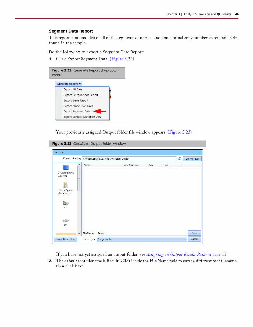
Segment Data ReportThis report contains a list of all of the segments of normal and non-normal copy number states and LOH found in the sample.
Do the following to export a Segment Data Report:
1. Click Export Segment Data. (Figure 3.22)
Your previously assigned Output folder file window appears. (Figure 3.23)
If you have not yet assigned an output folder, see Assigning an Output Results Path on page 11.
2. The default root filename is Result. Click inside the File Name field to enter a different root filename, then click Save.
Figure 3.22 Generate Report drop-down menu
Figure 3.23 OncoScan Output folder window

Chapter 3 | Analysis Submission and QC Results 45
A progress bar appears while your report generates, followed by a report finished successfully message, as shown in Figure 3.24.
3. Click Yes.
The OncoScan Output folder window appears.
4. Locate the Segment Data Report text file, then open it in Microsoft Excel.
The following window appears. (Figure 3.25)
Figure 3.24 Segment Data Report successful
Figure 3.25 Segment Data report

Chapter 3 | Analysis Submission and QC Results 46
Segment ID An Affymetrix identifier for the segment.
Chromosome Chromosome on which the probeset is located.
Start Position Start position of the segment.
End Position End position of segment.
Marker Count Number of markers in the segment.
Type Indicates if the segment is a copy number segment or an LOH segment.
State Indicates the copy number state of the segment for copy number segments or if the segment contains LOH for LOH segments (0=No, 1 = Yes).
Median Log2 Ratio Log2 Ratio is the log2 ratio of the normalized intensity of the sample over the normalized intensity of a reference with further correction for sample specific variation. The Median Log2 Ratio is computed for each segment.
Median BAF B-allele frequency (BAF) is (Signal (B)/{Signal(A) + Signal(B), where signal (A) is the signal from the AT chip and signal (B) is the signal from the G/C chip. Median BAF is computed for each segment and is the median BAF of the markers identified as heterozygous, after mirroring any marker BAFs above 0.5 to the equivalent value below 0.5. If the number of heterozygous markers in the segment is below 10 or the percent of homozygous markers is above 85% no value is reported.
% Aberr.Cells If % AC = 100%, we return “homogeneous” because it could be 100% normal or 100% tumor. If % AC =NA, the percent aberrant cells could not be determined and TuScan returns non-integer CN calls. This metric is an algorithmically determined estimate of the % of aberrant cells in the sample.
TuScan Ploidy TuScan Ploidy is the most likely ploidy state of the tumor before additional aberrations occurred. Algorithmically it is the CN state of the markers identified by the algorithm as normal diploid before %AC and ploidy are determined. When a high ploidy is determined the "normal diploid" is deemed to correspond to a higher CN and the log2 ratio gets adjusted appropriately. If ploidy cannot be determined NA (Not Available) is reported.
Filename Name of the OSCHP file containing the data

Chapter 3 | Analysis Submission and QC Results 47
Somatic Mutation Data Report
This report generates two (tab-delimited) text files; the somatic mutation file containing the call for each somatic mutation in the sample, and the somatic mutation annotation file containing annotation information for the somatic mutations assayed.
Do the following to export a Somatic Mutation Data Report:
1. Click Export Somatic Mutation Data. (Figure 3.26)
Your previously assigned Output folder file window appears. (Figure 3.23)
If you have not yet assigned an output folder, see Assigning an Output Results Path on page 11.
2. The default root filename is Result. Click inside the File Name field to enter a different root filename, then click Save.
NOTE: This report is not available for OncoScan_CNV.
Figure 3.26 Generate Report drop-down menu
Figure 3.27 OncoScan Output folder window
NOTE: The Export Somatic Mutation Data report produces two separate (tab-delimited)text files, as shown in the Files of type field. (Figure 3.27)
Chapter 3 | Analysis Submission and QC Results 48
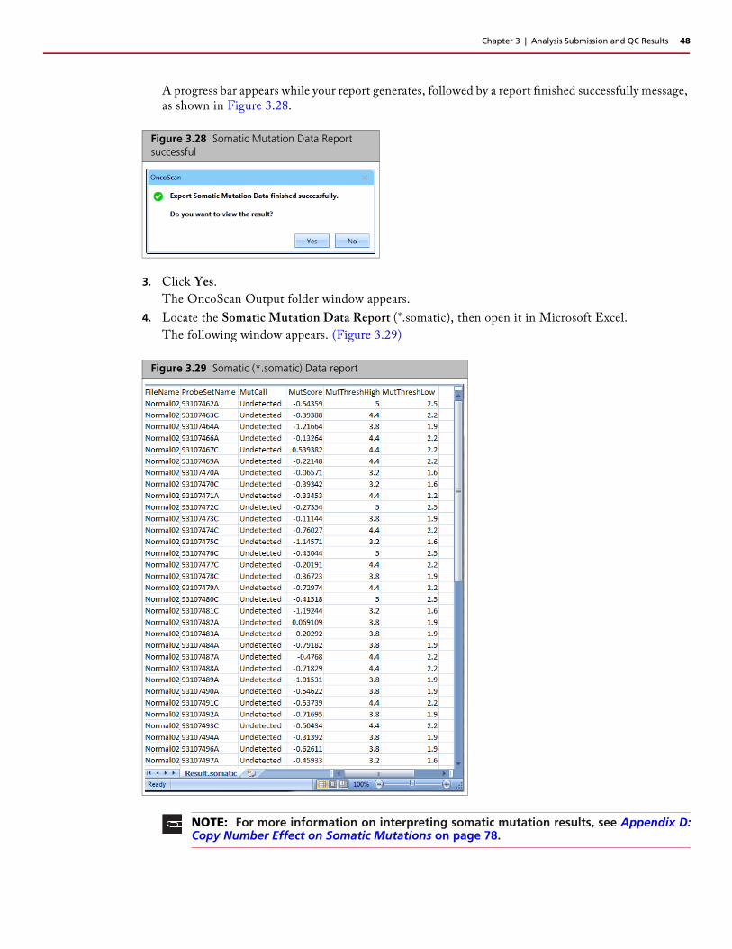
A progress bar appears while your report generates, followed by a report finished successfully message, as shown in Figure 3.28.
3. Click Yes.
The OncoScan Output folder window appears.
4. Locate the Somatic Mutation Data Report (*.somatic), then open it in Microsoft Excel.
The following window appears. (Figure 3.29)
Figure 3.28 Somatic Mutation Data Report successful
Figure 3.29 Somatic (*.somatic) Data report
NOTE: For more information on interpreting somatic mutation results, see Appendix D:Copy Number Effect on Somatic Mutations on page 78.

Chapter 3 | Analysis Submission and QC Results 49
5. From your OncoScan Output folder, locate the second Somatic Mutation Data Report (*.somaticannotation) text file, then open it in Microsoft Excel.
Filename Name of the OSCHP file containing the data
ProbeSetName Name of the probeset.
MutCall An indication of the whether the somatic mutation was decteded. A MutCall is displayed as Undetected if the MutScore is below the Low Confidence threshold. A MutCall is reported as HighConfidence if greater than or equal to the High Confidence threshold. If the MutCall is equal to or greater than the Low Confidence threshold and is less than the High Confidence threshold, the MutCall is reported as LowerConfidence.
Note: MutCalls from"Outside Bounds" samples are not reliable.
MutScore Measures somatic mutation probeset response. The stronger the response, the morelikely it is that the somatic mutation is present. The MutScore calculation dependson the algorithm version. The newer MutScore calculation also corrects for sample specificeffects, and thereby reduces false positive calls, which were sample specific.
For algorithm versions 1.0 - 1.2 (ChAS 3.0 and earlier, OncoScan Console 1.2 andearlier):
MutScore.old = (measured quantile normalized signal - median signal for this markerin the reference model file) / (95th percentile signal for this marker in the referencemodel file - median signal for this marker in the reference model file).
For algorithm versions 1.3 and newer (ChAS 3.1 and newer, releases of OncoScanConsole after 1.2):
MutScore.new = (MutScore.old - median MutScore.old for this sample) / standarddeviation of MutScore.old for this sample (where standard deviation is calculated forall but the num-out-std strongest MutScore.old for this sample, median is calculatedfor all but the num-out-med strongest MutScore.old for this sample, and the usedmedian is the maximum of zero and the measured median).
MutThreshHigh High confidence MutScore threshold. Measurements equal to or greater than this threshold are called "High confidence," describing the likelihood that the mutation is present.
MutThreshLow Lower confidence MutScore threshold. Measurements with a MutScore below this value are called "Undetected". Measurements equal to or greater than this threshold but less than the High Threshold are called "Lower confidence," describing the likelihood that the mutation is present.

Chapter 3 | Analysis Submission and QC Results 50
The following window appears. (Figure 3.30)
Figure 3.30 Somatic (*.somaticannotation) report
ProbeSetName Name of the probeset.
chr_id Chromosome on which the somatic mutation is found.
start Start position of the somatic mutation.
stop End position of the somatic mutation.
probeset_type Indicates if the probeset is used for Somatic Mutation analysis (SOM).
tag_id An Affymetrix identifier for the tag associated with the particular probeset.
common_id Abbreviated description of the mutations to which this ProbeSet is known to respond. The name has the form [Gene]:[amino acid change for mutation]:[cDNA change for mutation]. In the event that the ProbeSet cannot differentiate among multiple mutations to which it can respond, the slash (/) delimits the multiple known mutations.
cosmic_id The identifier of the mutation as listed in the COSMIC database, which is a catalogue of somatic mutations in cancer. More information on these mutations can be found at: http://cancer.sanger.ac.uk
channel The Channel file from which the signal is measured. "A" is the AT CEL, "C" is the GC CEL.

Chapter 3 | Analysis Submission and QC Results 51
Export All DataUse this option to generate all the reports (described in detail above) simultaneously.
1. Click Export All Data. (Figure 3.31)
The following window appears. (Figure 3.32)
2. Click to select the appropriate BED file, then click Open.
Your previously assigned Output folder file window appears. If you have not yet assigned an output folder, see Assigning an Output Results Path on page 11.
3. Enter a Root File Name for your text (tab-delimited) Export All Data file, then click Save.
Figure 3.31 Generate Report drop-down menu
Figure 3.32 Select the BED file for the Gene Report window
NOTE: As shown in Figure 3.32, the default OncoScan-specific BED file for the Gene reportis OncoScanGeneBoundaries.r1.bed. However, any BED file can be used to generate theGene Report on any regions of interest contained within the BED file.
NOTE: The default root filename is Result. Click inside the File Name field to enter adifferent root filename.

Chapter 3 | Analysis Submission and QC Results 52
A progress bar appears while your report generates, followed by a report finished successfully message, as shown in Figure 3.33.
4. Click Yes.
Your OncoScan Output folder window appears and shows all the reports generated from the Export All option. (Figure 3.34)
5. Open the text file report you want to view using Microsoft Excel.
Figure 3.33 Export All Data successful
Figure 3.34 Output folder window
Chapter 4
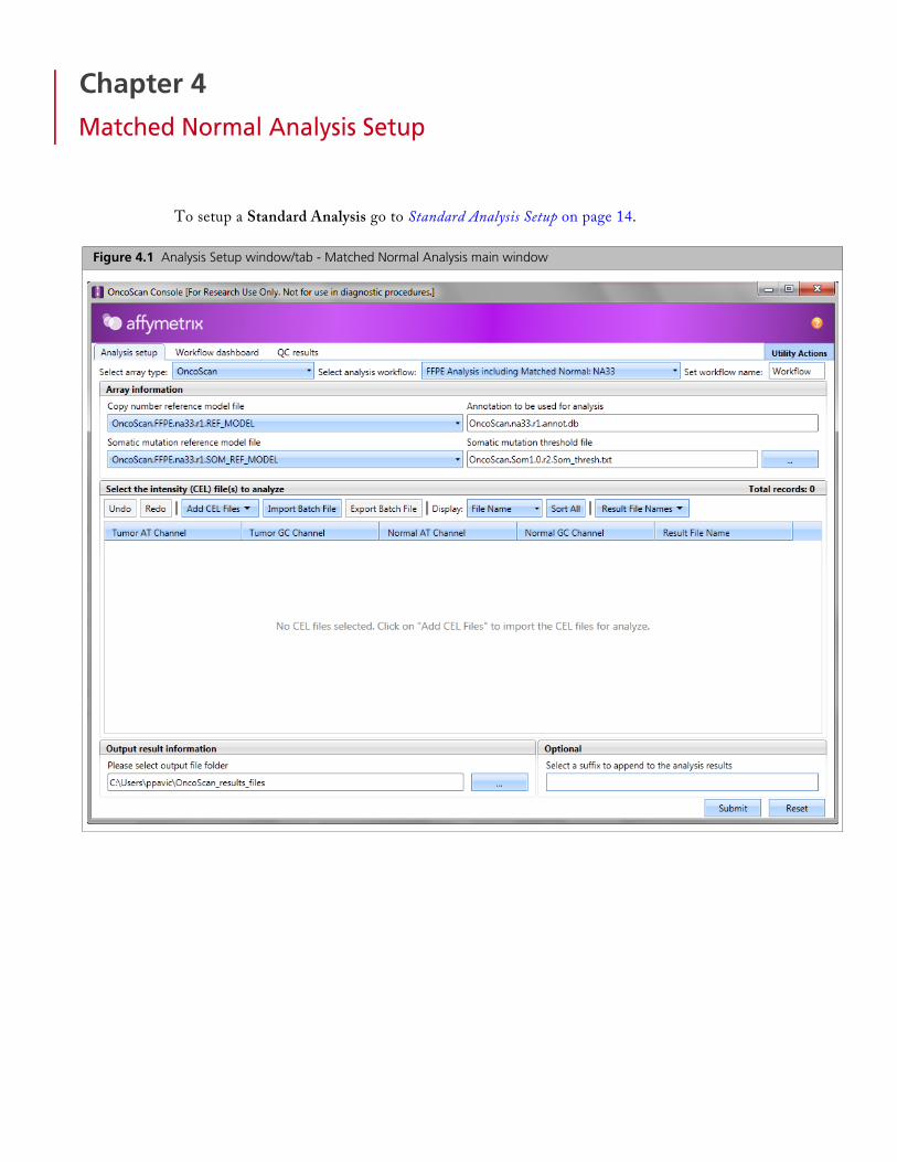
Matched Normal Analysis Setup
To setup a Standard Analysis go to Standard Analysis Setup on page 14.
Figure 4.1 Analysis Setup window/tab - Matched Normal Analysis main window

Chapter 4 | Matched Normal Analysis Setup 54
Selecting Array Information
1. From the Select array type drop-down list, click to select either OncoScan or OncoScan_CNV.
As long as your library file folder contains the necessary analysis files for the array, your configuration paths are established and your Array Information fields auto-populate, as shown in Figure 4.2.
Somatic mutation file selection is NOT available with the OncoScan_CNV array type, as shown in Figure 4.3.
2. From the Select analysis workflow drop-down list, click to select FFPE Analysis including Matched Normal NA33.
3. (Optional) Enter a Workflow name. By default, the Set workflow name is Workflow. Click (upper right) to enter a different workflow name.
The Annotation file is automatically selected for you and is based on your selected reference model file. (Example: OncoScan.na33.v1.annot.db)
4. Select a Somatic mutation reference model file. (OncoScan array only. Not applicable to OncoScan_CNV array.) By default, it is set to the previously used model file. If you created your own reference model file, click the drop-down list to select your .SOM_REF_MODEL.
Figure 4.2 Matched Normal Analysis Configuration - OncoScan array
Figure 4.3 Matched Normal Analysis Configuration - OncoScan_CNV array
NOTE: The Select array type drop-down list includes only the array types from the library (analysis) files that have been downloaded from NetAffx or copied from the Library package provided in the OncoScan installation package.
IMPORTANT: After adding new library files to the library file folder, always close and re-launch OncoScan Console to ensure the newly added files are recognized by the software.
TIP: Customizing a Workflow name can be a useful tool in keeping track of analysis workflows as all the related output files (outside of the OSCHP file) begin with this workflow name.
NOTE: The Annotation to be used for analysis field is auto-populated based on your Ref Model file selection. The analysis is not be permitted to run if the appropriate annotation file is not available in your Library folder.

Chapter 4 | Matched Normal Analysis Setup 55
5. Confirm the displayed Somatic mutation threshold file to be used is correct. If you need to change it, click the Browse button, navigate to the appropriate threshold .txt file, then click OK.
Adding CEL Files to AnalyzeYou can manually add CEL files or import them as a tab-delimited text file.
Manually Adding CEL Files to AnalyzeTo add batch-edited CEL files, see Importing CEL Files Using Batch Import on page 58.
To manually add CEL files:
1. At the Select the intensity (CEL) file(s) to analyze pane, click the Add CEL files drop-down.
2. Click Tumor AT Channel.
The CEL file window appears. (Figure 4.4)
IMPORTANT: If the Reference Model File and Somatic mutation Reference Model File were created independently of each other, a warning message appears after you click Submit (to start the Workflow Analysis process). Click OK to acknowledge the message.
Figure 4.4 CEL file folder -EXAMPLE

Chapter 4 | Matched Normal Analysis Setup 56
3. Click any header to sort your files or click the Files of type drop-down to filter your CEL files by AT Channel, as shown in Figure 4.5.
4. Single click, Ctrl click, or Shift click (to select multiple Tumor AT Channel files).
5. Click Open.
The Tumor AT Channel fields are now populated. (Figure 4.6)
6. Click the Add CEL files drop-down.
7. Click Tumor GC Channel. The CEL file window appears. (Figure 4.4 on page 55)
8. Single click, Ctrl click, or Shift click (to select multiple Tumor GC Channel files).
9. Click Open.
The Tumor GC Channel fields are now populated. (Figure 4.7)
10. Click the Add CEL files drop-down.
11. Click Normal AT Channel. The CEL file window appears. (Figure 4.4)
12. Single click, Ctrl click, or Shift click (to select multiple Normal AT Channel files).
13. Click Open.
Figure 4.5 Files of type drop-down list
IMPORTANT: Affymetrix recommends using an “A” or “C” as the last character to designate the channel in the CEL file naming convention. Example: “_AS_05A.CEL” is an AT Channel file, while “_AS_05C.CEL” is a GC Channel file. See Figure 4.4.
Figure 4.6 Tumor AT Channel file list
Figure 4.7 Tumor GC Channel file list

Chapter 4 | Matched Normal Analysis Setup 57
The Normal AT Channel fields are now populated. (Figure 4.8)
14. Click the Add CEL files drop-down.
15. Click Normal GC Channel. The CEL file window appears. (Figure 4.4)
16. Single click, Ctrl click, or Shift click (to select multiple Normal GC Channel files).
17. Click Open.
The Normal GC Channel fields are now populated. (Figure 4.9)
CEL File Displaying Options (Optional)The File Name drop-down list (Figure 4.10) is dynamically populated and based on what attributes are populated in the ARR file.
To use this display option, you must:
1. Provide the appropriate attributes at the time of sample registration in AGCC.
2. The ARR files must reside in the same folder as the CEL files.
To see “channel” (as an option in the drop down), you must use a template (or the OncoScan template provided in the library files) that contains a “channel” attribute. The resulting ARR file must also reside in the same folder as the CEL files you are analyzing.
You can display one of the attributes from the ARR file in the table. For example, “Channel” can be chosen (Figure 4.10) to confirm the assignment of a CEL file to its appropriate channel.
Figure 4.8 Normal AT Channel file list
Figure 4.9 Normal GC Channel file list
Figure 4.10 EXAMPLE: File Name Display Choices

Chapter 4 | Matched Normal Analysis Setup 58
To select a FIle Name display attribute:
1. Click the File Name drop-down button, then click to select the attribute you want displayed along with your CEL file names.
The two examples (Figure 4.11 and Figure 4.12) show how the table appears with the display set to Filename, then to Channel.
Importing CEL Files Using Batch ImportOncoScan Console allows import of CEL files using a batch file. The batch file must be saved as a text (Tab-delimited) format and include the full directory path for your CEL files (as shown in Figure 4.13).
The format for this tab-delimited file is 5 columns (A,B, C, D, and E) with the headers:
ATCHANNELCEL
GCCHANNELCEL
ATChannelMatchedNormalCel
GCChannelMatchedNormalCel
RESULT
You must provide the full path to the CEL files for each Channel column. (Example: C:\Desktop\OncoScan\Data\Sample1.cel)
Figure 4.11 Table with Filename displayed
Figure 4.12 Table with Channel displayed
TIP: The resulting OSCHP files are saved to your output path location, therefore it is not necessary to include a path under RESULT. Simply enter the desired results filename in this column.
Figure 4.13 List from Windows Excel

Chapter 4 | Matched Normal Analysis Setup 59
1. Click Import Batch File
A File window appears.
2. Navigate to your text (tab delimited) file location, then click on the file you want to import.
3. Click Open.
The Tumor AT, Tumor GC, Normal AT, Normal GC and Result File Name fields are now populated. (Figure 4.14)
Generating Result File NamesResults File Names can either be entered in manually or OncoScan Console can generate them automatically.
To manually enter a Results File Name:
1. Single-click inside the appropriate Results Name File field to produce a cursor, then type in the file name you want.
To auto-generate a suggested Result File Name:
1. After the 4 Channel lists are populated, click the Result File Names drop-down, then select Auto Generate Output Name.
IMPORTANT: The Microsoft Excel application must be closed before you import (click Open).
Figure 4.14 Tab-delimited text file imported into OncoScan Console
NOTE: If you use the suffix option (Selecting a Suffix to Append to the Analysis Results on page 62) and enter your Result File Names manually, your assigned suffix appears in the Results File Name column.
If you auto-generate your Results File Names, your assigned suffix appears in the Results File Name column, but it does get added to your final OSCHP file name(s).
NOTE: During the Result File Name auto-generation process, the file names are compared to identify their common root name for use as a results file name. Generally, the last 5 characters of each CEL file name are ignored, then the remaining root names of the AT and GC file names are compared. If the root names of the AT and GC channel match, then the root name is used in the Results File Name field. The one exception is if your array name “_(OncoScan)” is appended to the file name during registration in Affymetrix GeneChip Command Console (AGCC). In this case, the “_(OncoScan)” is ignored during the comparison, but then added back in the Results File Name field.

Chapter 4 | Matched Normal Analysis Setup 60
2. The Result File Name column is now populated with suggested filenames for each pairing. (Figure 4.15)
Common root names should be consistent all the way up to the last character of the CEL file name prior to the .cel extension. If there is a paired file mis-match, the Results File Name appears as Output1. (Figure 4.16)
If Output1 or subsequent Outputs (Output 2, Output 3...) appear, investigate the validity of your original pairing. See Correcting Mismatched CEL File Pairings on page 60.
To edit an auto-generated Result File Name:
1. Click on the Result File name you want to edit.
2. After the cursor appears, edit the filename as you normally would.
3. Click outside the row to save your edit.
To clear the entire Result File Name column:
1. Click the Result File Names drop-down button, then select Clear Column.
The column is now cleared and ready for new Result File Name entries.
Correcting Mismatched CEL File PairingsIf there is a paired file mismatch, the Results File Name appears as Output1, Output2, Output3, etc.
A paired file mismatch is most likely caused by an incorrect CEL filename pairing and not a mismatch of your native CEL files.
A simple way to correct mismatches is to sort the AT and GC columns so that files with the same root names are next to each other.
Using the Sorting Features
To sort an individual column:
1. Click on a Channel header.
The column is now sorted in an ascending order.
Figure 4.15 Matched Normal Results File Name list
Figure 4.16 Result File Name “Output”
TIP: Common root names should be consistent all the way up to the last character of the cel file name prior to the .cel extension. Affymetrix recommends using an “A” or “C” as the last character to designate the channel in the CEL file naming convention. Example: “_AS_05A.CEL” is an AT Channel file, while “_AS_05C.CEL” is a GC Channel file.

Chapter 4 | Matched Normal Analysis Setup 61
2. Click on the Channel header again to reverse the sorting order.
To sort all the columns simultaneously:
1. Click Sort All.
The file contents of the 4 columns are now sorted together in an ascending order.
2. Click Sort All again.
The file contents of the 4 columns are now sorted together in a descending order.
To swap CEL files between columns:
1. Click and drag a column CEL entry onto another column CEL entry, then release the mouse button.
The CEL entries have now swapped column positions.
To reorder the CEL files in a column:
1. Click and drag a CEL file to another position within the column, then release the mouse button.
The CEL file is now at its new position.
To add a cell to a column:
1. Click and drag a column cell to the top or bottom border line of a neighboring cell, then release the mouse button.
Generating a Result File Name after Sorting1. After all your columns are properly sorted, click the Result File Names drop-down, then select Auto
Generate Output Names.
The Result File Name column is now populated with suggested filenames for each pairing.
If OncoScan Console detects an inconsistency between the AT and GC file names to be paired, a Result File Name labeled, “Output n” reappears.
Repeat the sorting steps above, then try to Auto Generate Output Names again until a successful Result File Name(s) appears.
Setting your Output Information Location (Optional) The Output result information path (lower left) is retained from your initial setup.
To select a different folder to store your results:
1. Click the browse button, then navigate to the folder you want. If you want to change the default folder, see Assigning an Output Results Path on page 11.
NOTE: An OSCHP file is created for each pair. The tumor will have “_T” and the normal will have “_N” appended to its root name.
IMPORTANT: Confirm that both columns are sorted in the same direction. If they are, examine the files and confirm they are paired correctly. The file names (excluding the last character before the .CEL) MUST match exactly.
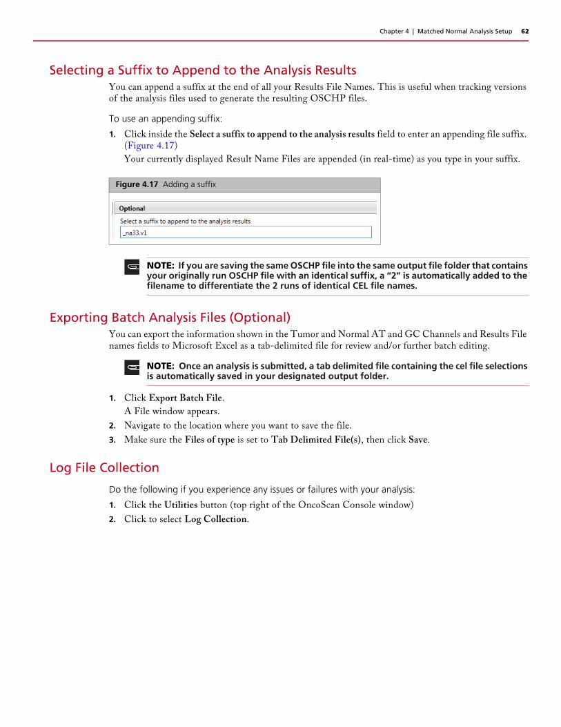
Chapter 4 | Matched Normal Analysis Setup 62
Selecting a Suffix to Append to the Analysis ResultsYou can append a suffix at the end of all your Results File Names. This is useful when tracking versions of the analysis files used to generate the resulting OSCHP files.
To use an appending suffix:
1. Click inside the Select a suffix to append to the analysis results field to enter an appending file suffix. (Figure 4.17)
Your currently displayed Result Name Files are appended (in real-time) as you type in your suffix.
Exporting Batch Analysis Files (Optional)You can export the information shown in the Tumor and Normal AT and GC Channels and Results File names fields to Microsoft Excel as a tab-delimited file for review and/or further batch editing.
1. Click Export Batch File.
A File window appears.
2. Navigate to the location where you want to save the file.
3. Make sure the Files of type is set to Tab Delimited File(s), then click Save.
Log File Collection
Do the following if you experience any issues or failures with your analysis:
1. Click the Utilities button (top right of the OncoScan Console window)
2. Click to select Log Collection.
Figure 4.17 Adding a suffix
NOTE: If you are saving the same OSCHP file into the same output file folder that contains your originally run OSCHP file with an identical suffix, a “2” is automatically added to the filename to differentiate the 2 runs of identical CEL file names.
NOTE: Once an analysis is submitted, a tab delimited file containing the cel file selections is automatically saved in your designated output folder.

Chapter 4 | Matched Normal Analysis Setup 63
The following window appears. (Figure 4.18)
3. Use OncoScan Console’s default location of C:\ or navigate to a folder location of your choice.
4. Click Create New Folder, then enter a folder name for your log.
5. Click OK.
The following window appears confirming your log file has been saved as a zip file.
Figure 4.18 Log Collection File window
Figure 4.19 Example: Zip file contents of a Log Collection

Chapter 4 | Matched Normal Analysis Setup 64
6. Click OK to close the window.
Viewing the Log Collection File
To view the log collection file:
1. Use Windows Explorer to navigate to the location. (Example: C:\ProgramData\Affymetrix\OncoScan\log)
2. Locate the zip folder you created earlier, then double-click on it.
The folder opens.
3. Extract the zipped folder’s contents, as you normally would. (Figure 4.20)
Log RolloverWhen the software determines that the log file for the Analysis Workflow (C:\ProgramData\Affymetrix\OncoScan\log\AnalysisWorkflow.log) has reached a defined size (approximately 4MB), the following steps will be completed:
A sub-folder will be created in C:\ProgramData\Affymetrix\OncoScan\log called 'Log*' (the '*' denotes the current date and time).
A zip file called RolledLogFile*.zip is created in that folder. The '*' is the same date and time used for the folder name. The files in the C:\ProgramData\Affymetrix\OncoScan\log folder and all files found in the currently selected QC History Log folder will be included in this zip file.
The Analysis Workflow files that are associated with analysis workflows that are no longer active on the Dashboard will be deleted from: C:\ProgramData\Affymetrix\OncoScan\log
A new AnalysisWorkflow.log file will be created here: C:\ProgramData\Affymetrix\OncoScan\log
NOTE: The auto-generated log collection zip file contains the full contents of the folder and all QC History log files found in the configured QC History File path. By default, the zip file resides here: C:\ProgramData\Affymetrix\Oncoscan\log
Figure 4.20 Example: Zip file contents of a Log Collection

Appendix A
Appendix A: Custom Reference Files
Creating your Own Reference File
1. From the Analysis Setup tab Select array type drop-down list, click to select an array type (Example: OncoScan) (Figure A.1)
2. From the Select analysis workflow drop-down list, click to select Reference Generation NA33.
3. By default, the Set workflow name is Workflow. Click (upper right) to enter a different workflow name.
4. Select the annotation File for this analysis to be used for analysis. (Example: OncoScan.na33.v1.annot.db)
After you create your reference file, navigate to your library file folder, then open the Signature SNPs Report text file. Confirm that the report shows that your sample pairings and channel IDs are correct.
If they are not, you must adjust the pairings and channel data in OncoScan Console’s Select the intensity (CEL) file(s) to analyze table (see Correcting Mismatched CEL File Pairings on page 18), then re-run the reference file.
IMPORTANT: When creating an OncoScan FFPE Assay reference file, you must use a minimum of six CEL files (including one male and one female). It is recommended that you select at least 44 normal samples of good quality. Ideally, your male and female samples should be of equal numbers (22 and 22).
Figure A.1 Reference File creation example
NOTE: The Select array type drop-down list includes only the array types for which library (analysis) files have been downloaded from NetAffx or copied from the Library package provided with the installation.

Appendix B
Appendix B: QC Metrics - Definitions
Array Data QC Metrics (Overview)This section provides a high level overview of the key QC metrics used with OncoScan Console.
MAPD (Median of the Absolute Values of all Pairwise Differences)MAPD is a global measure of the variation of all microarray probes across the genome. It represents the median of the distribution of changes in log2 ratio between adjacent probes. Since it measures differences between adjacent probes, it is a measure of short-range noise in the microarray data. Lower MAPD values are better. For more information, see Array Data QC Metrics (Detailed Descriptions) on page 69.
ndSNPQC (SNP Quality Control of Normal Diploid Markers)ndSNPQC is a measure of how well genotype alleles are resolved in the microarray data. The calculation only uses probesets that appear to be in normal diploid regions. Larger ndSNPQC values are better. For more information, see ndSNPQC on page 71.
SNP QC Type (SNP Quality Control Type)If SNP QC Type is ND, metrics like ndSNPQC, ndWavinessSD, ndSNR_AT, ndSNR_GC, ndRawSNPQC are all based on the performance of the normal diploid marker subset counted by ndCount. If SNP QC Type is non ND, then ndSNPQC and ndRawSNPQC are computed based on a preselected set of 10,000 autosomal markers, while ndWavinessSD are computed on all autosomal markers.
CelPairCheck StatusCelPairCheck is a test that inspects each pair of intensity (*.cel) files to determine whether the files have been properly paired and assigned to the correct channel. In addition to accidental mispairing of intensity files while setting up the analysis, a tracking problem during the assay may result in a sample being assigned to the wrong GeneChip array. As a result CelPairCheck ignores file names, and instead inspects the genotypes in the two intensity files to detect file mispairings. If the CelPairCheck Status is not Pass, see CelPairCheckStatus on page 73.
CelPairCheck Compare RateThis metric is the percentage of signature SNP control markers whose genotypes are compared between the AT and GC channels. The Compare Rate needs to be above a minimum in order for CelPairCheck to determine whether the AT and GC CEL files belong to the same individual.
CelPairCheck ConcordanceThis metric is the concordance of a set of signature SNP genotypes compared between AT and GC CEL files. If CelPairCheck Compare Rate is high but CelPairCheck Concordance is low, then CelPairCheck Status will report "PossibleCELmispair".
ndWavinessSD (Normal Diploid Waviness Standard Deviation)ndWavinessSD is a global measure of variation of microarray probes that is insensitive to short-range variation and focuses on long-range variation. ndWavinessSD is computed on normal diploid markers.

Appendix B | Appendix B: QC Metrics - Definitions 67
ndWavinessSD should be used along with Low Diploid Flag, ndCount (the actual number of diploid markers identified) BAFs, and log2 ratio to assess if the log2 ratio is centered correctly. ndWavinessSD can thus help assess if log2 ratios need to be re-centered.
In addition when ndWavinessSD is high, the log2 ratios should be examined for clear breakpoints as opposed to a gradual drift of the log2 ratio. When the latter is observed small aberrations should be examined carefully. When breakpoints are sharp and the ndCount is large a high ndWavinessSD can be ignored.
Y Gender CallGender call determined by examining signal on the Y Chromosome.
ndCountndCount reports how many normal diploid markers were identified. When ndCount falls below a minimum (typically 2000), the Low Diploid Flag is triggered. ndCount > 10,000 is desired for maximum confidence in ndSNPQC and maximum confidence in the centering of the log2 ratios.
Low Diploid FlagAn essential part of the algorithm is the identification of “normal diploid” markers in the cancer samples. This is particularly important in highly aberrated samples. The normal diploid markers are used to calibrate the signals so that “normal diploid markers” result in a log2 ratio of 0 (e.g. copy number 2). The algorithm might later determine that the "normal diploid" markers identified really correspond to (for example) CN=4. In this case the log2 ratio gets readjusted and TuScan ploidy will report 4. Occasionally (in about 2% of samples) the algorithm cannot identify a sufficient number of “normal diploid” markers and no normal diploid calibration occurs. This event triggers "Low Diploid Flag = Yes." In this case the user needs to carefully examine the log2 ratios and verify if re-centering is necessary.
ACDC (Aberrant Cell-Derived Copy Number)Indicates whether the algorithm was able to compute the % Aberr. Cells and measure the Copy Number in the tumor cells only. “ACDC= No” means Copy Number was calculated as an average CN across all cells, “ACDC=Yes” means that Copy Number was calculated only for the tumor cells.
%Aberr. CellsAlgorithmic estimation of the percent of aberrant cells (%AC) in a sample.
When %AC is “NA” it means that the % aberrant cells could not be estimated because the percent is either too low or the sample is heterogeneous and hence is composed of several types of aberrated cells, or the percent varies from one genomic location to another.
When %AC is not NA, (example 60%), it means that across all aberrations, ~60% of the cells were aberrated and contributed to the elevated (or reduced) Copy number.
TuScan PloidyTuScan Ploidy is the most likely ploidy state of the tumor before additional aberrations occurred. Algorithmically it is the CN state of the markers identified by the algorithm as normal diploid before %AC and ploidy are determined. When a high ploidy is determined the "normal diploid" is deemed to correspond to a higher CN and the log2 ratio gets adjusted appropriately. If ploidy cannot be determined NA (Not Available) is reported.

Appendix B | Appendix B: QC Metrics - Definitions 68
Reliability ScoreThis metric evaluates the fit between the actual and predicted log2 ratios and BAFs, and is only meaningful when ACDC = Yes. The predicted log2 ratios and BAFs are computed from the predicted TuScan Ploidy, %Aberr. Cells, and reported copy number states. Reliability Score ranges from 0 to 1.1, and values above 0.8 represent a good score. If Reliability Score cannot be calculated, "NA" is reported. Samples that are considered Within Bounds but have a low Reliability Score may have less reliable predictions for TuScan Ploidy, %Aberr. Cells, and reported copy number states.
Offset Flag If the Offset Flag is Yes, the TuScan results required an adjustment to the log2 ratios, as explained under TuScan Ploidy. As a result, allelic peaks, and smooth signal values get rescaled accordingly.
TuScan L2R AdjTuScan L2R Adj is the constant added by the TuScan algorithm to the log2 ratios, when the Offset Flag = Yes. Note: This value does not include any additional user adjustment when performing manual recentering.
Adjusted Log2 RatioThe median log2 ratio value entered by the user during manual recentering of a chromosome region the user wants to designate as diploid.
Low % Aberrant Cell nGoFGoodness of fit (GoF) is evaluated when TuScan tries to explain the CN changes by assuming a two state mixture model of normal and aberrant cells. A large nGoF value indicates an estimation of the % aberrant cells cannot be calculated, due to the aberrant cell fraction being below TuScan detection limits.
Hyb Control Intensity_ATGeometric mean of three array hybridization controls in the AT channel. An unusually low value indicates a problem at the array hybridization and/or washing step.
Hyb Control Intensity_GCGeometric mean of three array hybridization controls in the GC channel. An unusually low value indicates a problem at the array hybridization and/or washing step.
Q3 Raw Intensity_ATThe 75th percentile of the raw intensity of the AT channel.
Q3 Raw Intensity_GCThe 75th percentile of the raw intensity of the GC channel.
AGR_ATAntigenomic ratio in the AT channel. Measures non-specific binding to array features in that channel. Smaller values are better.
Appendix B | Appendix B: QC Metrics - Definitions 69
AGR_GCAntigenomic ratio in the GC channel. Measures non-specific binding to array features in that channel. Smaller values are better.
ndSNR_ATThis metric is the Signal/Noise Ratio of normal diploid markers in the AT channel. The Signal is the 65th percentile of the measurements used for copy number analysis, minus the median of the antigenomic features. The Noise is the standard deviation of the weakest 15% of measurements used for copy number analysis. A low value indicates poor data quality from the AT CEL file.
ndSNR_GCThis metric is the Signal/Noise Ratio of normal diploid markers in the GC channel. The Signal is the 65th percentile of the measurements used for copy number analysis, minus the median of the antigenomic features. The Noise is the standard deviation of the weakest 15% of measurements used for copy number analysis. A low value indicates poor data quality from the GC CEL file.
ndRawSNPQCLike ndSNPQC, but calculated on raw intensities.
Call RateThe percentage of snps for which a genotype could be determined - divided by the total number of snps. The higher the Call Rate, the better. Call rate is based on genotype calls using an algorithm which assumes all autosomal markers are normal diploid. Therefore, this metric is more relevant for normal samples than for aberrated tumor samples.
Matched Normal Compare RateIf doing FFPE analysis including matched normal (where you supply four CEL files per row during analysis setup), this metric reports the percentage of markers identified as normal diploid in both the resulting Tumor OSCHP file, and its matched Normal OSCHP file. If this metric is unusually low, then the results of the companion metric Matched Normal Concordance may be unreliable.
Matched Normal ConcordanceIf doing FFPE analysis including matched normal (where you supply four CEL files per row during analysis setup), this metric reports the genotype concordance of the normal diploid markers in common between the Tumor OSCHP file and its matched Normal OSCHP file. If the Matched Normal Compare Rate is reasonably high but Matched Normal Concordance is low, then the normal CEL files you paired with the tumor CEL files may not belong to the same individual. This metric is only reported for the Tumor OSCHP file.
Array Data QC Metrics (Detailed Descriptions)
MAPDFor quality assessment purposes, we define metrics that assess whether the microarray data is of sufficient quality to accurately assess copy number (CN) analysis. One of these metrics is Median of the Absolute values of all Pairwise Differences (MAPD).

Appendix B | Appendix B: QC Metrics - Definitions 70
MAPD is defined as the Median of the Absolute values of all Pairwise Differences between log2 ratios for a given chip. Each pair is defined as adjacent in terms of genomic distance, with SNP markers and CN markers being treated equally. Hence, any two markers that are adjacent on the genome are a pair. Except at the beginning and the end of a chromosome, every marker belongs to two pairs, as shown in Figure B.1.
Formally, if xi: is the log2 ratio for marker i:
MAPD = median(|xi-1 – xi|, with i ordered by genomic position)
MAPD is a per-microarray estimate of variability, like standard deviation (SD) or interquartile range (IQR). If the log2 ratios are distributed normally with a constant SD, then MAPD/0.96 is equal to SD and MAPD*1.41 is equal to IQR. However, unlike SD or IQR, using MAPD is robust against high biological variability in log2 ratios induced by conditions such as cancer.
Variability in log2 ratios in a microarray arises from two distinct sources:
Intrinsic variability in the starting material, hybridization cocktail preparation, microarray or scanner
Apparent variability induced by the fact that the reference may have systematic differences from this microarray
Regardless of the source of the variability, increased variability decreases the quality of CN calls.
Effect of MAPD on Functional PerformanceAs a measure of performance, we measured copy number gains and loss using over 1000 cancer samples. Arrays with MAPD > 0.3 are out of bounds.
ndWaviness-SDWaviness refers to an effect seen in all genomic microarrays (see Maroni et al. (2007) Genome Biology 8:R228) where long-range variation is observed, often associated with regional genomic differences like local GC-content changes.
This metric is only computed on markers that have been identified as Normal diploid by the algorithm. When Low Diploid Flag = Yes, ndWaviness-SD is computed for all autosomal markers. For most samples, a ndWaviness-SD value below 0.12 for OncoScan arrays indicates that the long-range variation is within levels that can be accommodated by the algorithms.
ndWavinessSD should be used along with LowDiploidFlag, ndCount (the actual number of diploid markers identified) BAFs and log2 ratio to assess if the log2 ratio is centered correctly. ndWavinessSD can thus help assess if log2 ratios need to be re-centered.
In addition when ndWavinessSD is high, the log2 ratios should be examined for clear breakpoints as opposed to a gradual drift of the log2 ratio. When the latter is observed small aberrations should be examined carefully. When breakpoints are sharp and the ndCount is large a high ndWavinessSD can be ignored.
Figure B.1 Example: Two pairs to a marker

Appendix B | Appendix B: QC Metrics - Definitions 71
ndSNPQCThe ndSNPQC metric estimates the distributions of homozygous AA, heterozygous AB and homozygous BB alleles and calculates the distance between them. The better the separation of these distributions, the better the ability to identify a genotype based on its cluster position, as shown in Figure B.2.
SNPQC correlates well with genotype performance, as measured by Call Rate and Concordance to published HapMap genotypes.
For OncoScan, we use ndSNPQC. This is computed only on the normal diploid markers to assess the quality of the genotypes and the resulting quality of BAFs. When Low Diploid Flag = Yes, ndSNPQC is computed for a preselected set of 10,000 autosomal markers. As a result, values may fall out of bounds although the data quality is good. We therefore recommend always examining the BAF visually when Low Diploid Flag = Yes and ndSNPQC is out of bounds.
Effect of ndSNPQC on Functional Performance ndSNPQC provides insight into the overall level of data quality from a SNP perspective. The key consideration when evaluating the ndSNPQC value is to ensure the threshold is exceeded. The quality of the SNP allele data is compromised, and is noisier and more difficult to interpret when the ndSNPQC values are below the recommended acceptance threshold as illustrated in the figure below.
When the ndSNPQC value is below 26, the noise within the array is higher than normal which compromises the overall clarity of results. ndSNPQC values above 26 have good data quality and can be relied upon with regards to performance as shown in Figure B.3. Sometimes ndSNPQC values can be as high as 35 (or higher) and provide even better separation of BAFs.
Figure B.2 Example: Genotype based on its cluster position

Appendix B | Appendix B: QC Metrics - Definitions 72
Figure B.3 Examples: (TOP) Sample with Noisier BAFs. (BOTTOM) Sample with clearly delineated BAFs.

Appendix B | Appendix B: QC Metrics - Definitions 73
CelPairCheckStatus
Most of the probes in the OncoScan assay are designed so that each OncoScan array detects only one of the two alleles for a specific SNP, and so both arrays are needed to measure a full genotype call for that SNP. However a set of control probes are included so that both alleles for a set of “Signature SNPs” can be measured on each array independently.
The pattern of genotype calls for these Signature SNPs is compared between the two intensity files. As the signature SNPs are a set of high minor allele frequency SNPs, under normal assay conditions it is very unlikely that two unrelated tested samples will have the same pattern of Signature SNP genotype calls. Therefore, if the concordance of genotype calls is unusually low between a given pair of intensity files, the CelPairCheck Status message will be "PossibleCELmispair." The concordance check is only done if there are enough Signature SNPs reporting a call in both files. If this is not the case, CelPairCheck Status reports “Warn.”
Signature SNP probes are designed to be channel-specific. When an intensity file is assigned to the AT channel, only the Signature SNP probes designed to respond in the assay's AT reaction well are expected to report genotypes. In the case of GC data being assigned to the AT channel for analysis, a low call rate will result in the CelPairCheck Status message “PossibleGCinATchannel.” If AT data were assigned to the GC channel, the message would be "PossibleATinGCchannel."
If you need additional help fixing the problems detected by CelPairCheck Status, you can review that Signature SNP metrics and genotypes for each intensity file in the CelPairCheckReport file. This report is created along with result files (*.oschp) for each analysis, or go to OncoScan Console’s QC results tab, click on the Generate Report button, then select Export [CelPairCheck Report]. See Generating and Exporting Reports on page 35 for more details.
CelPairCheckStatus message Description
Pass No intensity file pairing problem is detected.
PossibleCELmispair Low genotype concordance exists between data in AT channel and data in GC channel. This is consistent with the data in the two inten-sity files originating from different individuals.
This message may also appear with poor data. Please review the chan-nel-specific sample QC metrics to see if one or both CEL files has a problem.
PossibleGCinATchannel Data from the GC reaction appears to be assigned to the AT analysis channel.
PossibleATinGCchannel Data from the AT reaction appears to be assigned to the GC analysis channel.
Warn Cannot determine whether the two intensity files belong to the same individual.
This message may appear with poor data, or with good data where too many of the signature SNPs used for CelPairCheck are in chromo-some regions with copy number aberrations.

Appendix B | Appendix B: QC Metrics - Definitions 74
ndWavinessSD For OncoScan we compute Waviness-SD on markers identified by the algorithm as “normal diploid” markers. It is a QC metric that focuses on measuring long-range effects. As described separately, MAPD is a metric that measures short-range variation, the variation of adjacent probes. The long-range variation measurement is accomplished by calculating the variation in log2 ratios across the whole genome and subtracting out the short-range variation, specifically, for autosomal probes:
Define:
Xi as the log2 ratios of autosomal probes
And Zi as the variance between adjacent probes:
Zi = X2i+1 - X2i
Waviness-SD is the total variance (Xi) minus the local variance (Zi):
Waviness-SD = sqrt(Var(Xi)-Var(Zi)/2)
% Aberrant CellsIf % AC = 100%, we return “homogeneous” because it could be 100% normal or 100% tumor. If % AC =NA, the percent aberrant cells could not be determined and TuScan returns non-integer CN calls.
The cause could be:
1. Low % aberrant cells
2. Low number of diploid regions
3. Data Quality, in particular for all samples for which MAPD is above 0.4 or ndSNPQC falls below 19.
4. Occasionally High/Low Ploidy
5. No Ploidy solution has a good fit to the data.
Low Diploid FlagAn essential part of the algorithm is the identification of “normal diploid” markers in the cancer samples. This is particularly important in highly aberrated samples. The normal diploid markers are used to calibrate the signals so that “normal diploid markers” result in a log2 ratio of 0 (e.g. copy number 2). The algorithm might later determine that the "normal diploid" markers identified really correspond to (for example) CN=4. In this case, the log2 ratio gets readjusted and TuScan ploidy will report 4. Occasionally (in about 2% of samples) the algorithm cannot identify a sufficient number of “normal diploid” markers and no “normal diploid calibration occurs. This event triggers “low diploid flag” = YES. In this case the user needs to carefully examine the log2 ratios and verify if re-centering is necessary.
Appendix C
Appendix C: Algorithms
B-allele FrequenciesB-allele frequencies (BAFs) are a graphical way to show allelic imbalances. BAFs are also used by the algorithm to derive the CN state. Conceptually for each marker we compute (Signal (B)/{Signal(A) + Signal(B), where signal (A) is the signal from the AT chip and signal (B) is the signal from the G/C chip. A homozygous BB SNP will therefore have a value of 1, a homozygous AA SNP a value of zero and a AB SNP a value of 0,5. For SNPS with high Minor allele frequency the BAFs present as three equally thick bands around these values (0, 0.5, 1).
In regions of Loss of heterozygosity the only possible alleles are BB and AA and the middle band (corresponding to AB) is missing.
In regions of Copy Gain the allelic balance is disrupted. With 3 copies it is not possible to have an equal amount of A and B alleles, and the BAF bands are at 0, 1/3, 2/3 and 1.
In cancer samples the additional complication of normal contamination of the tumor cells affects the allelic imbalance further.
When 60% of the cells have CN=3 and 40% of the cells have CN=2 the location of the BAF bands is at (0.6*2+0.4)/(3*0.6+2*0.4) =0.615, while it is at 0.66 (or 2/3) when 100% of the cells have CN=3. In general when the percent aberrated cells is p and the CN for these aberrated cells is 3 then, the middle BAF band shifts up to (2p+(1-p))/(3p+2(1-p)) an down to 1- (2p+(1-p))/(3p+2(1-p)).
LOH AlgorithmThe LOH algorithm uses B-allele frequencies (BAFs) and log2 ratios to find long stretches of homozygosity.
TuScan AlgorithmThe TuScan algorithm uses B-allele frequencies (BAFs) and log2 ratios to estimate the ploidy and percentage of aberrant cells in the sample (%AC) which in turn are used to calculate copy number calls (CN). The BAFs and log2 ratios contribute equally to CN determination. TuScan first uses the BAFs and log2 ratio data to identify segments of equal CN. Next TuScan uses the BAFs, log2ratios and segment data to find the combination of %AC and ploidy that best fits the data. When TuScan can successfully determine %AC, the algorithm assigns each aberrant segment an integer copy number representing the copy number in the tumor portion of the sample. This is possible because CN is well approximated by an integer when the tumor is nearly homogeneous. If the tumor is highly heterogeneous (i.e., lacks a dominant clone), or contains a large amount of “normal” cells %AC cannot be determined. In other words, if the percentage of aberrant cells contributing to the various aberrations in the sample varies across all aberrations, %AC and ploidy cannot be determined. When %AC cannot be determined, the segmentation algorithm will still identify segments of equal CN, but the CN in just the aberrant cells cannot be determined. In this case, TuScan bins the copy numbers and returns fractional CN values in 1/3 increments (e.g., 2, 2.33, 2.66, 3 etc.). This fractional copy number is derived from the normal contamination as well as the heterogeneous population of tumor cells; therefore, the fractional CN calls represent the average CN observed for that segment. Users should look at the value of %AC to determine whether the CN value represents the CN in the tumor (%AC= number) or the average CN in the sample (%AC=NA). Tumor heterogeneity also affects the interpretation of the CN number calls when %AC cannot be determined. For example, a TuScan call of 2.33 can result from 40% of the aberrant cells having 3 copies, 10% of aberrant cells having 5 copies, or a more complex heterogeneous mixture of copy numbers. Since nearly every tumor sample will have some amount of normal contamination combined with tumor heterogeneity it is not possible to predict how often TuScan will be able to determine the %AC, it will vary depending on the sample.

Appendix C | Appendix C: Algorithms 76
Figure C.1 Example: TuScan results as displayed in OncoScan Nexus Express
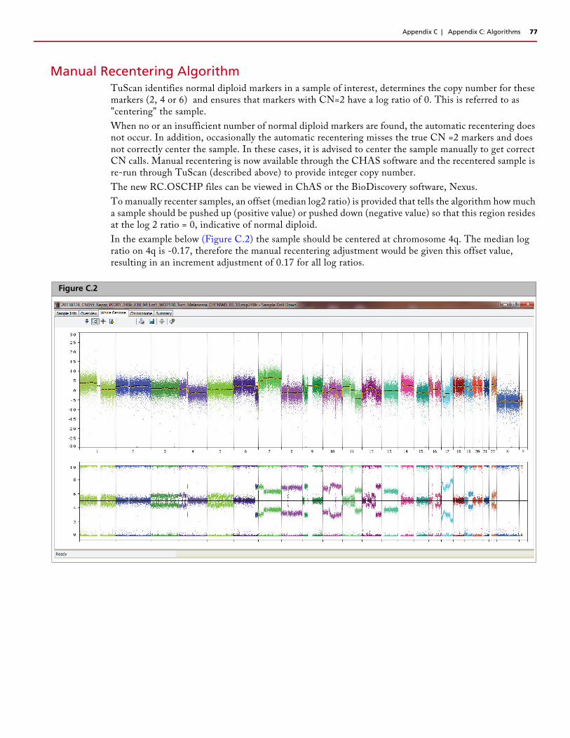
Appendix C | Appendix C: Algorithms 77
Manual Recentering AlgorithmTuScan identifies normal diploid markers in a sample of interest, determines the copy number for these markers (2, 4 or 6) and ensures that markers with CN=2 have a log ratio of 0. This is referred to as "centering" the sample.
When no or an insufficient number of normal diploid markers are found, the automatic recentering does not occur. In addition, occasionally the automatic recentering misses the true CN =2 markers and does not correctly center the sample. In these cases, it is advised to center the sample manually to get correct CN calls. Manual recentering is now available through the CHAS software and the recentered sample is re-run through TuScan (described above) to provide integer copy number.
The new RC.OSCHP files can be viewed in ChAS or the BioDiscovery software, Nexus.
To manually recenter samples, an offset (median log2 ratio) is provided that tells the algorithm how much a sample should be pushed up (positive value) or pushed down (negative value) so that this region resides at the log 2 ratio = 0, indicative of normal diploid.
In the example below (Figure C.2) the sample should be centered at chromosome 4q. The median log ratio on 4q is -0.17, therefore the manual recentering adjustment would be given this offset value, resulting in an increment adjustment of 0.17 for all log ratios.
Figure C.2
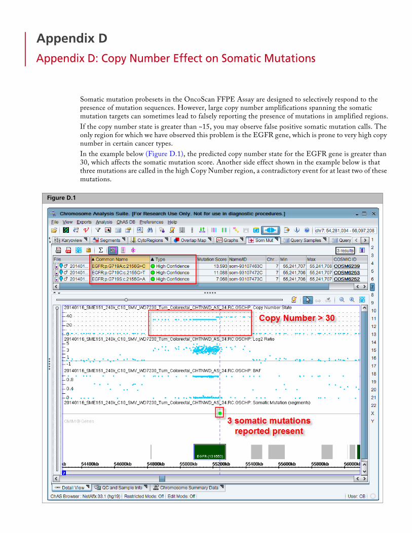
Appendix D
Appendix D: Copy Number Effect on Somatic Mutations
Somatic mutation probesets in the OncoScan FFPE Assay are designed to selectively respond to the presence of mutation sequences. However, large copy number amplifications spanning the somatic mutation targets can sometimes lead to falsely reporting the presence of mutations in amplified regions.
If the copy number state is greater than ~15, you may observe false positive somatic mutation calls. The only region for which we have observed this problem is the EGFR gene, which is prone to very high copy number in certain cancer types.
In the example below (Figure D.1), the predicted copy number state for the EGFR gene is greater than 30, which affects the somatic mutation score. Another side effect shown in the example below is that three mutations are called in the high Copy Number region, a contradictory event for at least two of these mutations.
Figure D.1