User’s Guide for Stata & SAS · SAS: The example sas file can be found in Appendix C. The example...
40
User’s Guide for Stata & SAS
Transcript of User’s Guide for Stata & SAS · SAS: The example sas file can be found in Appendix C. The example...

User’s Guide for Stata & SAS
StatTag Version 2.0 User’s Guide
2 | P a g e
Table of Contents
1.0 Introduction ......................................................................................................................... 3
2.0 Setup .................................................................................................................................... 4
3.0 Basics of StatTag .................................................................................................................. 5
3.1 Build ..................................................................................................................................... 6
3.2 Manage .............................................................................................................................. 13
3.3 Support............................................................................................................................... 17
4.0 Tag Structure and Syntax ................................................................................................... 17
4.1 Values ................................................................................................................................. 17
4.2 Tables ................................................................................................................................. 18
4.3 Figure ................................................................................................................................. 18
4.4 Syntax ................................................................................................................................. 18
5.0 Formatting tags .................................................................................................................. 19
5.1 Values ................................................................................................................................. 19
5.2 Tables ................................................................................................................................. 19
5.3 Formatting after insertion ................................................................................................. 20
6.0 Troubleshooting ................................................................................................................. 20
7.0 Acknowledgements ............................................................................................................ 22
Appendix A. Example Word Document for Stata ......................................................................... 23
Appendix B. Example Stata do file ................................................................................................ 24
Appendix C. Example SAS sas file .................................................................................................. 26
Appendix D. The display command .............................................................................................. 31
Appendix E. The matrix list command .......................................................................................... 34
Appendix F. The graph export command ..................................................................................... 36
Appendix G. The %put command ................................................................................................. 37
Appendix H. The ODS CSV and ODS PDF commands .................................................................... 38
Appendix I. Licenses ...................................................................................................................... 39
StatTag Version 2.0 User’s Guide
3 | P a g e
1.0 Introduction
StatTag is user-friendly software that integrates statistical code with document preparation in Microsoft Word. StatTag facilitates reproducible research by connecting Word documents, such as a manuscript, to associated statistical code. Word documents prepared with StatTag are reproducible dynamic documents: statistical results in the document can be automatically updated if either statistical code or data change. In addition, StatTag allows statistical code to be edited directly from Microsoft Word. StatTag is provided as a free Word plug-in written in C#. Once installed, StatTag is accessible from the Word toolbar. This user’s guide covers use of StatTag within a Windows environment for Microsoft Word partnered with Stata (StataCorp. 2015. Stata Statistical Software: Release 14. College Station, TX: StataCorp LP) and SAS (SAS. 2002-2012. SAS Institute Inc: Release 9.4. Cary, NC) statistical software. Future versions of StatTag will allow use of statistical code written for other programming software (R) as well as use within a Mac operating system.
StatTag Version 2.0 User’s Guide
4 | P a g e
2.0 Setup
For use with all statistical software, the StatTag plug-in must be installed. For some software, additional steps are required.
Setup Instruction
Install the StatTag Plugin Steps 1-3 Steps 1-3
Enable the Stata Automation API1 Steps 4-8
Install the StatTag Plug-In:
1. Download the StatTag setup.exe file.
2. When prompted, click “Run” and follow the InstallShield Wizard.
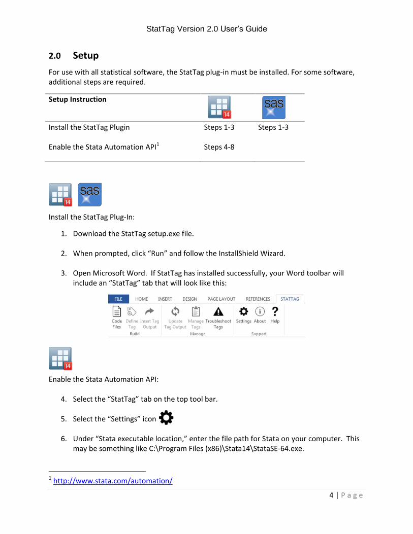
3. Open Microsoft Word. If StatTag has installed successfully, your Word toolbar will include an “StatTag” tab that will look like this:
Enable the Stata Automation API:
4. Select the “StatTag” tab on the top tool bar.
5. Select the “Settings” icon
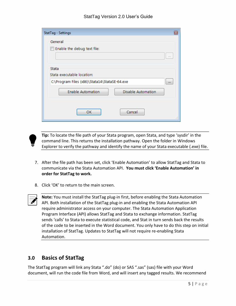
6. Under “Stata executable location,” enter the file path for Stata on your computer. This may be something like C:\Program Files (x86)\Stata14\StataSE-64.exe.
1 http://www.stata.com/automation/
StatTag Version 2.0 User’s Guide
5 | P a g e
Tip: To locate the file path of your Stata program, open Stata, and type ‘sysdir’ in the command line. This returns the installation pathway. Open the folder in Windows Explorer to verify the pathway and identify the name of your Stata executable (.exe) file.
7. After the file path has been set, click ‘Enable Automation’ to allow StatTag and Stata to communicate via the Stata Automation API. You must click ‘Enable Automation’ in order for StatTag to work.
8. Click ‘OK’ to return to the main screen.
Note: You must install the StatTag plug-in first, before enabling the Stata Automation API. Both installation of the StatTag plug-in and enabling the Stata Automation API require administrator access on your computer. The Stata Automation Application Program Interface (API) allows StatTag and Stata to exchange information. StatTag sends ‘calls’ to Stata to execute statistical code, and Stat in turn sends back the results of the code to be inserted in the Word document. You only have to do this step on initial installation of StatTag. Updates to StatTag will not require re-enabling Stata Automation.
3.0 Basics of StatTag
The StatTag program will link any Stata “.do” (do) or SAS “.sas” (sas) file with your Word document, will run the code file from Word, and will insert any tagged results. We recommend
StatTag Version 2.0 User’s Guide
6 | P a g e
that you begin with a do or sas file that already contains your working statistical code and generates the results of interest. With StatTag, it is possible to write your statistical code directly from Word, but not as convenient as writing your do files in the statistical program’s editor.
There are three main steps to using StatTag:
1. Connect a Word document to files containing statistical code (i.e. do or sas file).
2. Annotate the code files to tag results, tables, or figures that are of interest.
3. Instruct StatTag where to insert those results within the Word document itself.
Note: This guide uses example .do and .sas files to explain the use of StatTag. To follow along with the User Guide, copy the example code in Appendix B or C into a do or sas file on your own computer. Stata: The example do file can be found in Appendix B. The example do file uses the built in Stata dataset, bpwide, which is available to all Stata users, containing blood pressure data on 120 individuals. SAS: The example sas file can be found in Appendix C. The example sas file uses built in SAS datasets drug, bodyfat and normtemp, which are available to all SAS users.
3.1 Build
The three steps above are accomplished using the first three icons listed on the StatTag toolbar: Code Files, Define Tag, and Insert Tag Output. These three icons comprise the Build section of the StatTag toolbar. They allow the user to: (1) link statistical code to the Word document; (2) tag results, tables, and figures within the statistical code; and (3) identify where those tagged results should be inserted in to the Word document.
Code File
The Build toolbar enables linking one or more code files (i.e. do or sas file) with your Word document. The first step to using StatTag is to connect your Word document with your statistical code. Note that it is possible to connect multiple code files to one Word document, and you may use code files from both Stata and SAS in a single document. To link a code file:
1. Click on “Code Files”
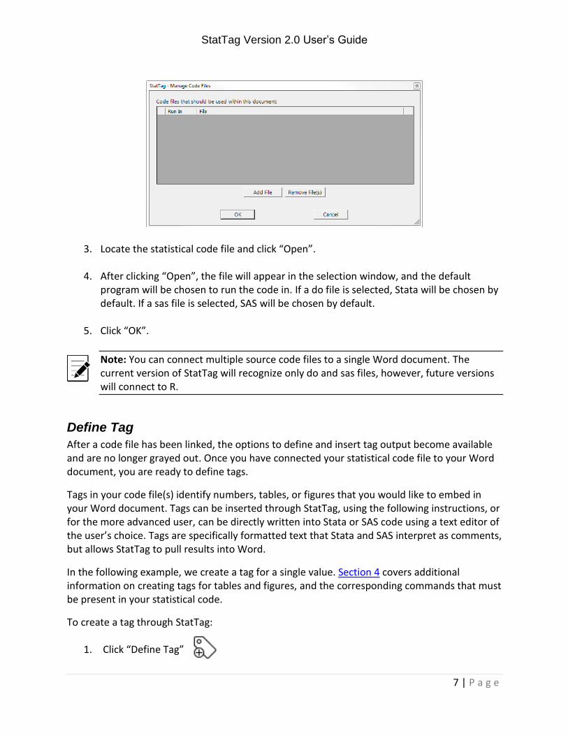
2. A new dialog box will open. Select “Add File”. A Windows Explorer box will open, allowing you to navigate to the appropriate code file. For the current version, this should be a Stata .do file or a SAS .sas file. Future versions of StatTag will allow R files.
StatTag Version 2.0 User’s Guide
7 | P a g e
3. Locate the statistical code file and click “Open”.
4. After clicking “Open”, the file will appear in the selection window, and the default program will be chosen to run the code in. If a do file is selected, Stata will be chosen by default. If a sas file is selected, SAS will be chosen by default.
5. Click “OK”.
Note: You can connect multiple source code files to a single Word document. The current version of StatTag will recognize only do and sas files, however, future versions will connect to R.
Define Tag
After a code file has been linked, the options to define and insert tag output become available and are no longer grayed out. Once you have connected your statistical code file to your Word document, you are ready to define tags.
Tags in your code file(s) identify numbers, tables, or figures that you would like to embed in your Word document. Tags can be inserted through StatTag, using the following instructions, or for the more advanced user, can be directly written into Stata or SAS code using a text editor of the user’s choice. Tags are specifically formatted text that Stata and SAS interpret as comments, but allows StatTag to pull results into Word.
In the following example, we create a tag for a single value. Section 4 covers additional information on creating tags for tables and figures, and the corresponding commands that must be present in your statistical code.
To create a tag through StatTag:
1. Click “Define Tag”
StatTag Version 2.0 User’s Guide
8 | P a g e
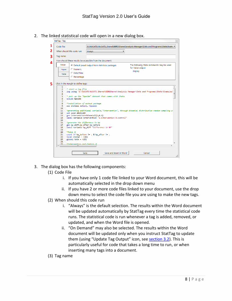
2. The linked statistical code will open in a new dialog box.
3. The dialog box has the following components: (1) Code File
i. If you have only 1 code file linked to your Word document, this will be automatically selected in the drop down menu
ii. If you have 2 or more code files linked to your document, use the drop down menu to select the code file you are using to make the new tags.
(2) When should this code run i. “Always” is the default selection. The results within the Word document
will be updated automatically by StatTag every time the statistical code runs. The statistical code is run whenever a tag is added, removed, or updated, and when the Word file is opened.
ii. “On Demand” may also be selected. The results within the Word document will be updated only when you instruct StatTag to update them (using “Update Tag Output” icon, see section 3.2). This is particularly useful for code that takes a long time to run, or when inserting many tags into a document.
(3) Tag name
1 2
3
4
5
StatTag Version 2.0 User’s Guide
9 | P a g e
i. The tag name is the unique name of the result of interest, and should only be used once within each code file to identify a result. StatTag will warn you if you try to use a tag name more than once.
ii. The tag name can contain any string of characters including special characters and spaces.
(4) Selection pane i. This section informs StatTag if the tag will be a value, figure, or table, and
how the data should be managed. ii. More information on tags for tables and figures is provided in section 4.
(5) Text editor showing the statistical code i. The statistical code may be edited directly though StatTag. Any changes
you make are made to the file itself and saved immediately.
4. Enter a tag name for your new tag. For this example, we will create a new tag called “Total N”, which will insert the total number of participants in the example study.
5. Use the text editor window to locate the statistical result of interest.
Note: StatTag recognizes different keywords in Stata and SAS. Use of these commands is discussed in detail in section 4 and Appendices D-H.
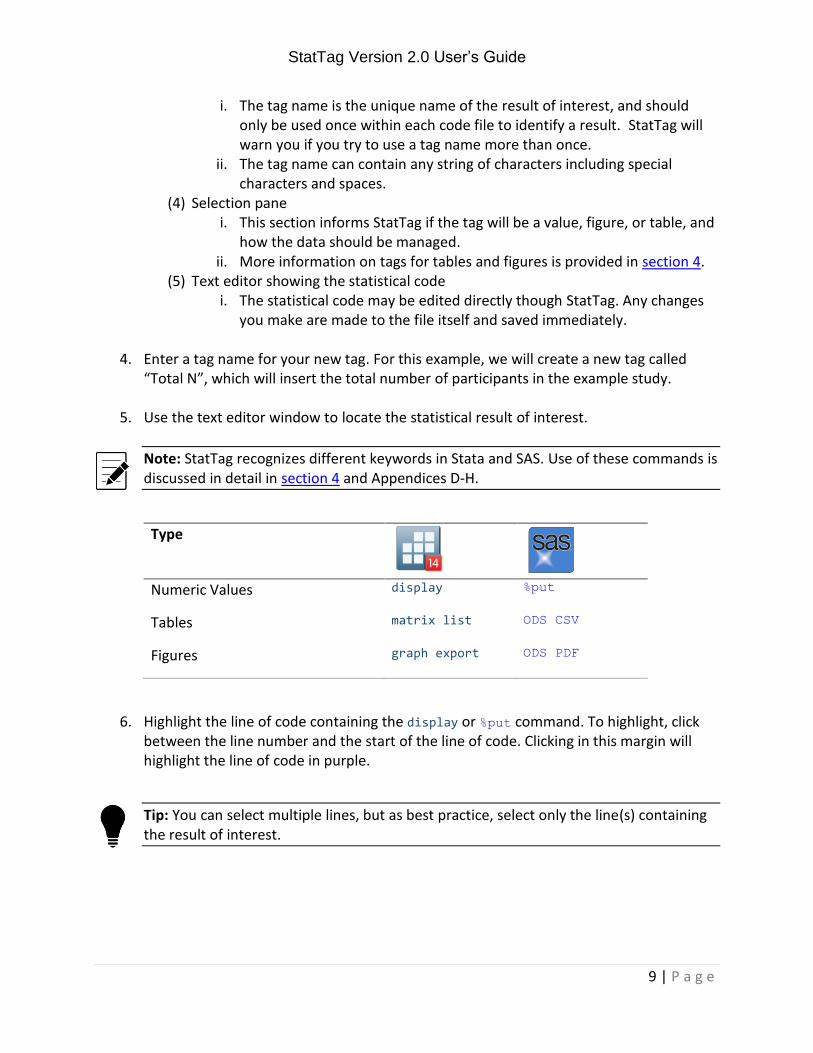
Type
Numeric Values display %put
Tables matrix list ODS CSV
Figures graph export ODS PDF
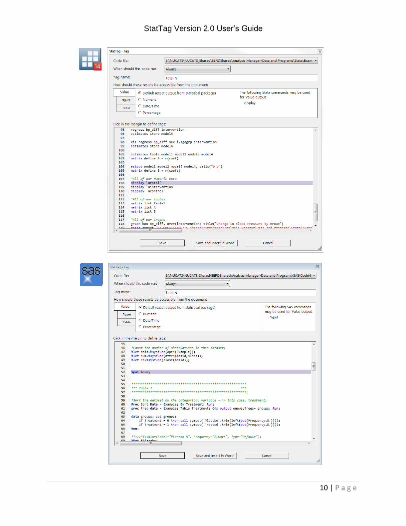
6. Highlight the line of code containing the display or %put command. To highlight, click between the line number and the start of the line of code. Clicking in this margin will highlight the line of code in purple.
Tip: You can select multiple lines, but as best practice, select only the line(s) containing the result of interest.
StatTag Version 2.0 User’s Guide
10 | P a g e
StatTag Version 2.0 User’s Guide
11 | P a g e
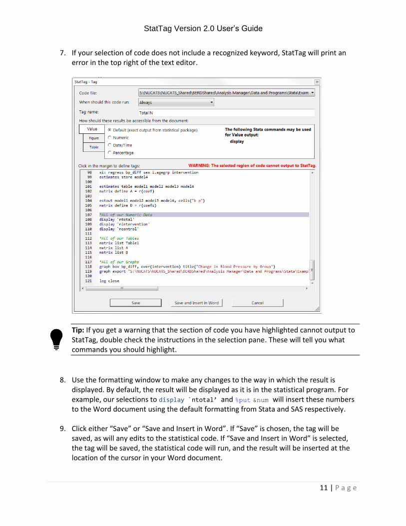
7. If your selection of code does not include a recognized keyword, StatTag will print an error in the top right of the text editor.
Tip: If you get a warning that the section of code you have highlighted cannot output to StatTag, double check the instructions in the selection pane. These will tell you what commands you should highlight.
8. Use the formatting window to make any changes to the way in which the result is displayed. By default, the result will be displayed as it is in the statistical program. For example, our selections to display `ntotal’ and %put &num will insert these numbers to the Word document using the default formatting from Stata and SAS respectively.
9. Click either “Save” or “Save and Insert in Word”. If “Save” is chosen, the tag will be saved, as will any edits to the statistical code. If “Save and Insert in Word” is selected, the tag will be saved, the statistical code will run, and the result will be inserted at the location of the cursor in your Word document.
StatTag Version 2.0 User’s Guide
12 | P a g e
10. Use the “Define Tag” icon as often as needed to create tags for all of your statistical results. (In the next section, we have also defined “Intervention N” and “Control N,” following the steps above).
Insert Tag Output
Tags can be inserted at the point of the cursor when they are defined, using the “Save and Insert in Word” option. They can also be inserted after they are created through the “Insert Tag Output” icon. Tags can be inserted more than once, and the results will be updated collectively throughout the text. Tags are always inserted at the location of the cursor, although they can be copied and pasted elsewhere once inserted.
Tip: Once a tag is inserted into a Word document, double clicking on the tag will open the tag window, from which you can modify the characteristics of the tag (name, when to run) or the associated statistical code.
To insert a saved tag:
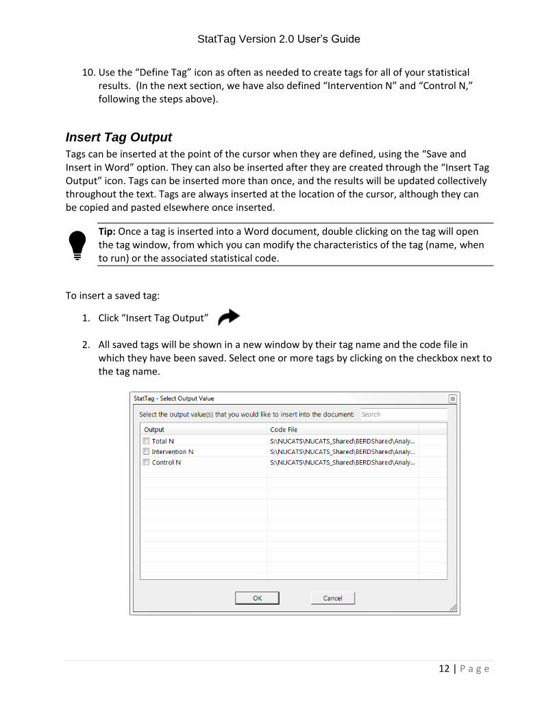
1. Click “Insert Tag Output”
2. All saved tags will be shown in a new window by their tag name and the code file in which they have been saved. Select one or more tags by clicking on the checkbox next to the tag name.
StatTag Version 2.0 User’s Guide
13 | P a g e
3. Click “OK” to insert the output. Upon clicking “OK” the statistical code will run and the result will be inserted in to the document.
3.2 Manage
The second portion of the StatTag toolbar consists of the Manage icons. These icons allow the user to manage tags after they have been created and inserted using the Build icons. The Manage icons include Update Tag Output, Manage Tags, and Troubleshoot Tags. These icons allow the user to manually update results; add, edit or delete saved tags, and troubleshoot any issues with inserted tags.
Update Tag Output
Tags are either updated “Always” when the statistical code is run (when new tags are defined, removed, or modified, and when the document is opened), or “On Demand” when the user instructs StatTag to update the results. To change how tags are updated, or to update the tags “On Demand”:
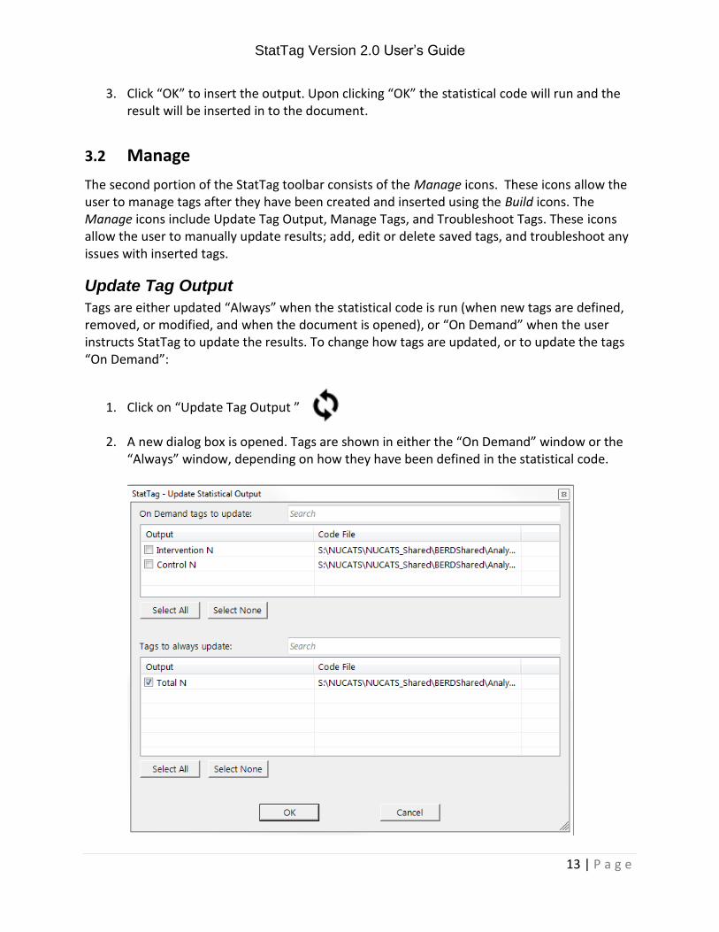
1. Click on “Update Tag Output ”
2. A new dialog box is opened. Tags are shown in either the “On Demand” window or the “Always” window, depending on how they have been defined in the statistical code.
StatTag Version 2.0 User’s Guide
14 | P a g e
3. To update the inserted results from any tags that have been defined as “On Demand,”
select the tags by checking the box next to the tag name.
4. To update the inserted results from any tags that have been defined as “Always,” select the tags by checking the box next to the tag name. By default, all of these tags will be selected.
5. Click “OK” to run the statistical code, and update the selected results.
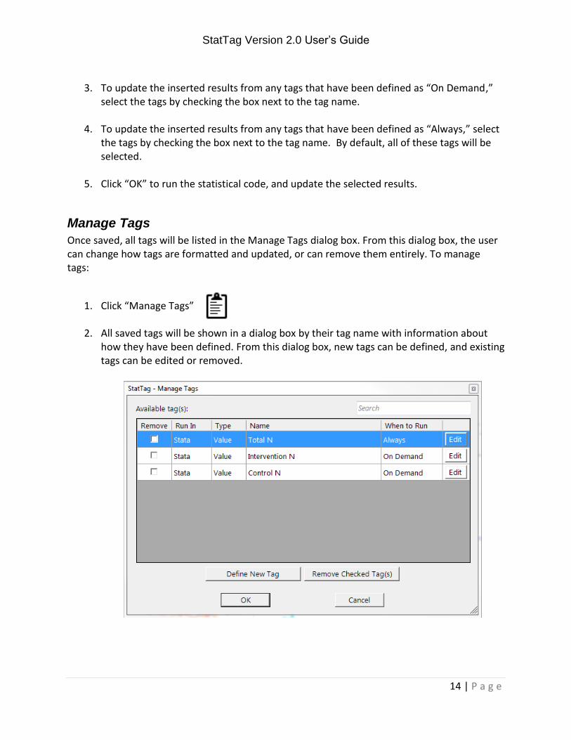
Manage Tags
Once saved, all tags will be listed in the Manage Tags dialog box. From this dialog box, the user can change how tags are formatted and updated, or can remove them entirely. To manage tags:
1. Click “Manage Tags”
2. All saved tags will be shown in a dialog box by their tag name with information about how they have been defined. From this dialog box, new tags can be defined, and existing tags can be edited or removed.
StatTag Version 2.0 User’s Guide
15 | P a g e
3. To define a new tag, click the “Define New Tag” button at the bottom of the dialog box. This will open the statistical code, and follow the “Define Tag” process described above. Defining new tags will insert new tag notation in your statistical code.
4. To edit a tag, click the “Edit” button on the right of the window. This opens the statistical code, showing the highlighted tag. The options for this tag can be edited through the dialog box.
5. To remove a tag, check the boxes next to each tag you wish to remove. Then click “Remove Checked Tag(s)”.
Note: Removing tags will delete the tag notation in your statistical code. Removing tags will not delete inserted text, tables or figures from your Word document. However, those results will no longer be tagged. They will not be updated when code is rerun or the document is open.
6. Click “OK” to permanently save any changes you have made within your statistical code.
Troubleshoot Tags
There are two troubleshoot options provided: (1) linking unlinked tags, and (2) removing duplicate tags. Tags can become unlinked if the statistical code is unlinked from the Word document, or if the statistical code is edited outside of StatTag and the notations are modified. For example, code could become unlinked if the do or sas file is moved to new location without changing the code file path in StatTag. Tag names can be duplicated within statistical code if the code is edited outside of StatTag and a tag name is inadvertently duplicated. To troubleshoot either issue:
1. Click “Troubleshoot Tags”
2. A new window will open showing any unlinked tags and any duplicated tags in separate tabs.
3. If there are unlinked tags, they will be shown in the first tab.
StatTag Version 2.0 User’s Guide
16 | P a g e
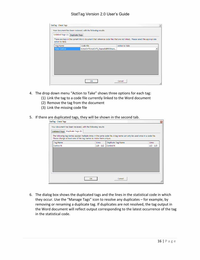
4. The drop down menu “Action to Take” shows three options for each tag: (1) Link the tag to a code file currently linked to the Word document (2) Remove the tag from the document (3) Link the missing code file
5. If there are duplicated tags, they will be shown in the second tab.
6. The dialog box shows the duplicated tags and the lines in the statistical code in which they occur. Use the “Manage Tags” icon to resolve any duplicates – for example, by removing or renaming a duplicate tag. If duplicates are not resolved, the tag output in the Word document will reflect output corresponding to the latest occurrence of the tag in the statistical code.
StatTag Version 2.0 User’s Guide
17 | P a g e
3.3 Support
Settings
The Settings window includes information about the StatTag version installed, the location of a debug file (if enabled) and if you are using Stata, maps the location of your Stata executable file. The debug file can be used to capture information about the StatTag plug in. If you encounter errors and would like to request assistance: (1) enable the debug file, which will write a plain text file to your computer; (2) run your program to generate the errors, and; (3) send the debug file to [email protected].
About
The About icon will open a window containing the version number of StatTag that you are using, and information regarding usage and licenses related to StatTag.
Help
The Help icon will open the User Guide from within Word. If you need additional help or support, email [email protected] or visit the StatTag website at http://sites.northwestern.edu/stattag/ to interact with the user community.
4.0 Tag Structure and Syntax
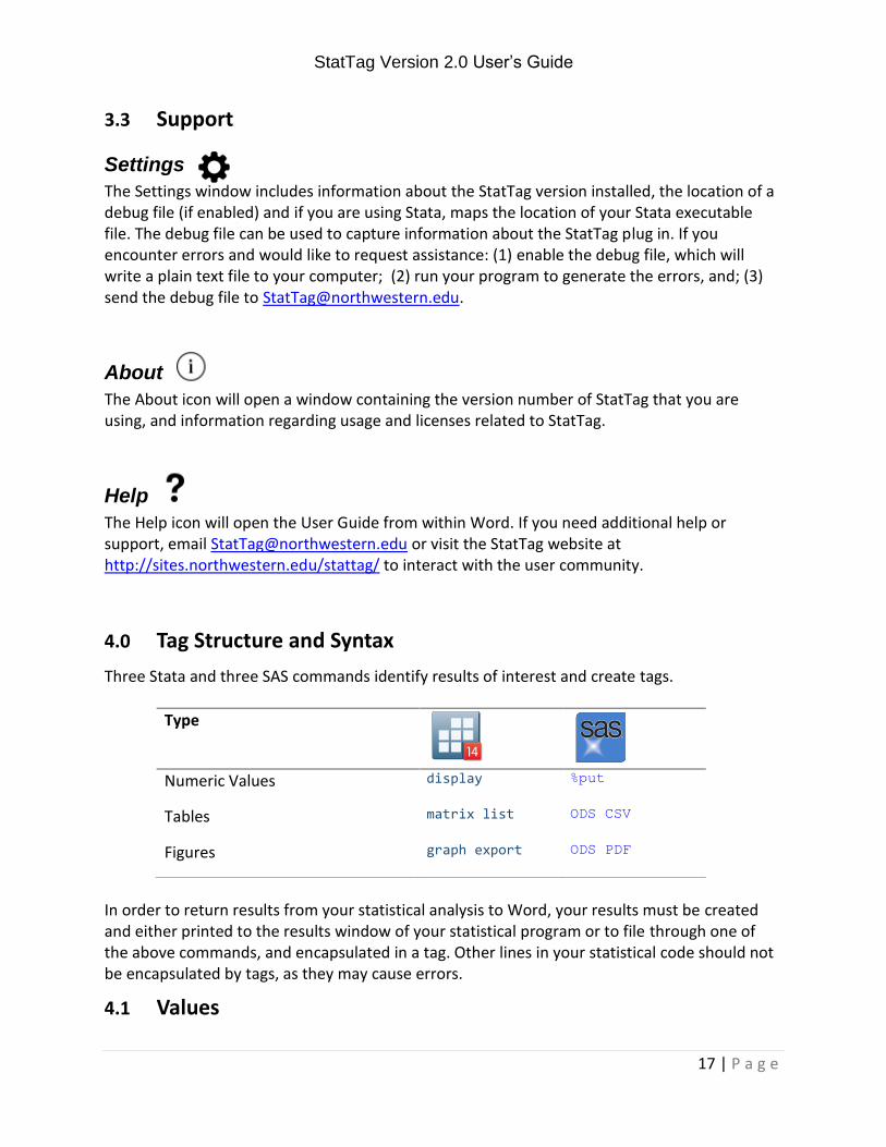
Three Stata and three SAS commands identify results of interest and create tags.
Type
Numeric Values display %put
Tables matrix list ODS CSV
Figures graph export ODS PDF
In order to return results from your statistical analysis to Word, your results must be created and either printed to the results window of your statistical program or to file through one of the above commands, and encapsulated in a tag. Other lines in your statistical code should not be encapsulated by tags, as they may cause errors.
4.1 Values
StatTag Version 2.0 User’s Guide
18 | P a g e
Values are returned to StatTag and then inserted into Word with the display (Stata) or %put (SAS) commands. These commands are used in Stata and SAS code to print strings or scalar values to the results window. They will not return data in any other format, such as a matrix or table.
The display command is typically used in Stata code with the return command to retrieve stored results, or with local or global macro variables. Examples of the display command are shown in Appendix D.
The %put command is typically used in SAS code to store values or strings as local macro variables. Examples of the %put command are shown in Appendix G.
4.2 Tables
Tables are returned to Word with the matrix list (Stata) or ODS CSV (SAS) commands.
The matrix list command is used in Stata code to print a matrix to the results window. The matrix list command is typically used after creation of a matrix with the mkmat, matrix define, estout, or estimates table commands. Examples of the matrix list command are shown in Appendix E.
The ODS CSV command is used in SAS code to redirect output to a location on file, instead of the results window. The file location is used by StatTag to pull in the results of interest. Examples of the ODS CSV command are shown in Appendix H.
4.3 Figure
Figures are returned to Word with the graph export (Stata) or ODS PDF (SAS) commands.
The graph export command is used in Stata code to save a graph or figure to file outside of Stata, the location of which is specified by the user. StatTag will retrieve the file to insert into Word. The graph export command expects a pathway and file name to be specified along with the file format, and the replace option to overwrite an existing file as required. The command will export the last graph rendered in Stata. Examples of the graph export command are shown in Appendix F.
The ODS PDF command is used in SAS code to save results of other commands to a pdf file outside of SAS, the location of which is specified by the user. StatTag will retrieve the file to insert into Word. The ODS PDF command expects a pathway and file name to be specified. The command will export any contained output that would be otherwise printed in the results window. Examples of the ODS PDF command are shown in Appendix H.
4.4 Syntax
A tag always starts with **>>>ST:Value(Label=" ", Frequency="",…) and may contain additional information based on the type of tag (number, table, or figure) it identifies. The tag
StatTag Version 2.0 User’s Guide
19 | P a g e
always ends with **<<<. Examples of tags for a numeric value, a table, and a figure are listed below. **>>>ST:Value(Label=" ", Frequency="", Type="")
code **<<< **>>>ST:Table(Label="", Frequency="", Type="", AllowInvalid=True, Decimals=0, Thousands=False)
code **<<< **>>>ST:Figure(Label="", Frequency="")
code **<<<
If tags are made through StatTag, the text (“***>>> …. **<<<”) will be written into your statistical code by the plug-in. The Label, Frequency, Type and Table parameters are inserted with the opening and closing tags by StatTag. For the more advanced user, you can also directly write tags into your statistical code. If written by hand in the statistical code, you must write both the opening and closing tags, and provide a tag name for each tag.
Note: Tags cannot be nested within each other. A tag should encapsulate exactly one keyword command (i.e. display, matrix list, %put, etc.)
5.0 Formatting tags
When a tag is created, its format should be specified accordingly. Options may be selected for either Values or Tables. There are no formatting options for Figures.
5.1 Values
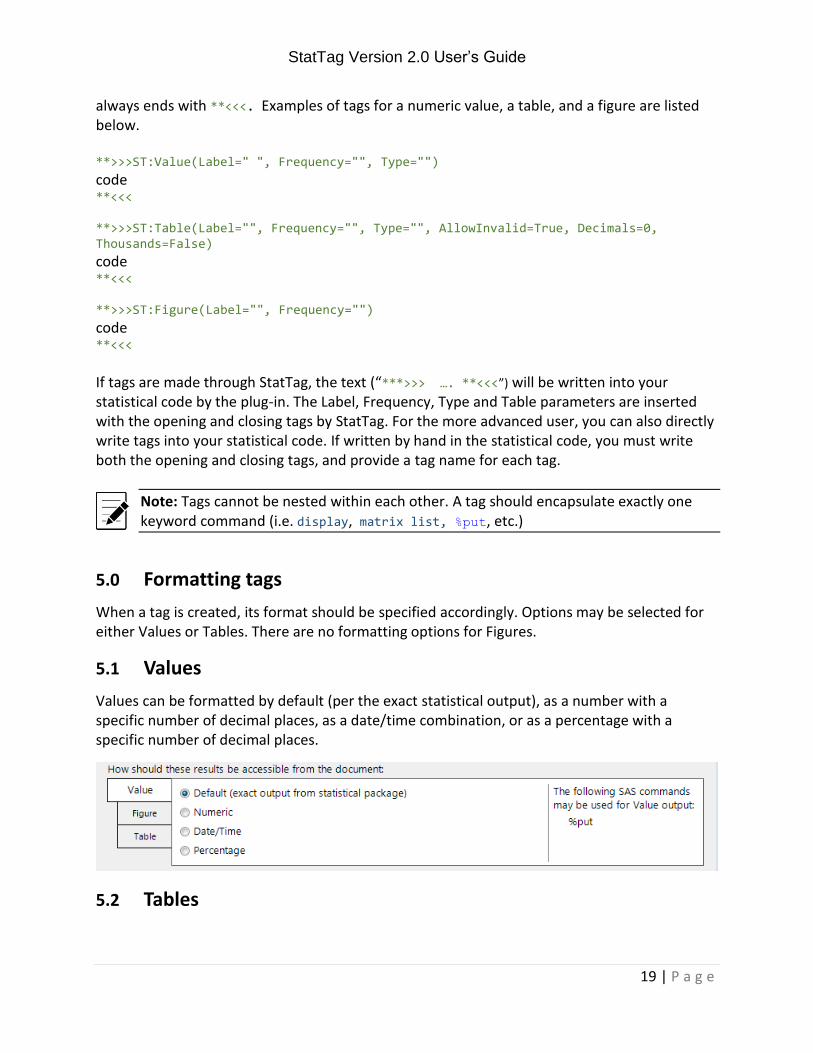
Values can be formatted by default (per the exact statistical output), as a number with a specific number of decimal places, as a date/time combination, or as a percentage with a specific number of decimal places.
5.2 Tables
StatTag Version 2.0 User’s Guide
20 | P a g e
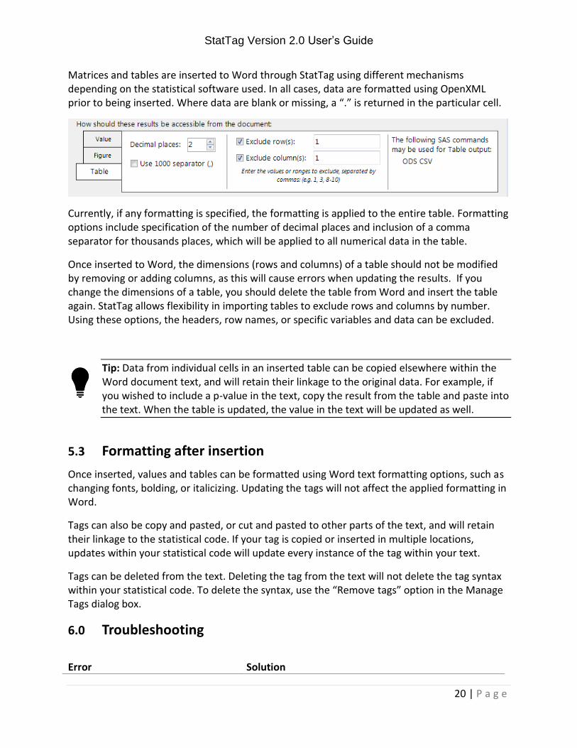
Matrices and tables are inserted to Word through StatTag using different mechanisms depending on the statistical software used. In all cases, data are formatted using OpenXML prior to being inserted. Where data are blank or missing, a “.” is returned in the particular cell.
Currently, if any formatting is specified, the formatting is applied to the entire table. Formatting options include specification of the number of decimal places and inclusion of a comma separator for thousands places, which will be applied to all numerical data in the table.
Once inserted to Word, the dimensions (rows and columns) of a table should not be modified by removing or adding columns, as this will cause errors when updating the results. If you change the dimensions of a table, you should delete the table from Word and insert the table again. StatTag allows flexibility in importing tables to exclude rows and columns by number. Using these options, the headers, row names, or specific variables and data can be excluded.
Tip: Data from individual cells in an inserted table can be copied elsewhere within the Word document text, and will retain their linkage to the original data. For example, if you wished to include a p-value in the text, copy the result from the table and paste into the text. When the table is updated, the value in the text will be updated as well.
5.3 Formatting after insertion
Once inserted, values and tables can be formatted using Word text formatting options, such as changing fonts, bolding, or italicizing. Updating the tags will not affect the applied formatting in Word.
Tags can also be copy and pasted, or cut and pasted to other parts of the text, and will retain their linkage to the statistical code. If your tag is copied or inserted in multiple locations, updates within your statistical code will update every instance of the tag within your text.
Tags can be deleted from the text. Deleting the tag from the text will not delete the tag syntax within your statistical code. To delete the syntax, use the “Remove tags” option in the Manage Tags dialog box.
6.0 Troubleshooting
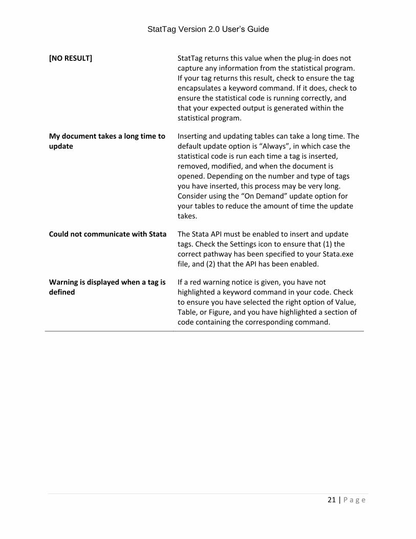
Error Solution
StatTag Version 2.0 User’s Guide
21 | P a g e
[NO RESULT] StatTag returns this value when the plug-in does not capture any information from the statistical program. If your tag returns this result, check to ensure the tag encapsulates a keyword command. If it does, check to ensure the statistical code is running correctly, and that your expected output is generated within the statistical program.
My document takes a long time to update
Inserting and updating tables can take a long time. The default update option is “Always”, in which case the statistical code is run each time a tag is inserted, removed, modified, and when the document is opened. Depending on the number and type of tags you have inserted, this process may be very long. Consider using the “On Demand” update option for your tables to reduce the amount of time the update takes.
Could not communicate with Stata The Stata API must be enabled to insert and update tags. Check the Settings icon to ensure that (1) the correct pathway has been specified to your Stata.exe file, and (2) that the API has been enabled.
Warning is displayed when a tag is defined
If a red warning notice is given, you have not highlighted a keyword command in your code. Check to ensure you have selected the right option of Value, Table, or Figure, and you have highlighted a section of code containing the corresponding command.

StatTag Version 2.0 User’s Guide
22 | P a g e
7.0 Acknowledgements
Development of StatTag and this user’s guide was supported, in part, by the National Institutes of Health's National Center for Advancing Translational Sciences, Grant Number UL1TR001422. The content is solely the responsibility of the developers and does not necessarily represent the official views of the National Institutes of Health. StatTag was inspired in part by the Stata Automation Report project:
Lo Magno, G.L. (2013). Sar: Automatic generation of statistical reports using Stata and Microsoft Word for Windows. The Stata Journal, 13(1); 39-64.
StatTag makes use of the following open source projects (licenses in Appendix I):
Scintilla - http://www.scintilla.org/
ScintillaNET - https://github.com/jacobslusser/ScintillaNET
Json.NET - http://www.newtonsoft.com/json
Use of these projects does not imply endorsement of StatTag by the respective project owners, or endorsement of the use of these projects by Northwestern University.
StatTag Version 2.0 User’s Guide
23 | P a g e
Appendix A. Example Word Document for Stata
Instructions: 1. After installation of StatTag, copy and paste the Stata code in Appendix B into a Stata do
file, “Example Do.do”. 2. Link a new Word document with the “Example Do.do” file. 3. Create a tag for the number of participants in the trial (Row 17)
The returned values should be: 120
4. Create a tag for Table 1 (Row 80) The returned table should look like:
control1 control2 int1 int2 pval
sex_=_0 29.00 0.24 31.00 0.26 0.71
sex_=_1 27.00 0.22 33.00 0.28 .
agegrp_=_1 23.00 0.19 17.00 0.14 0.13
agegrp_=_2 19.00 0.16 21.00 0.17 .
agegrp_=_3 14.00 0.12 26.00 0.22 .
bp_before 155.09 10.65 157.64 11.96 0.22
bp_after 149.80 13.78 152.72 14.48 0.26
bp_diff -5.29 15.51 -4.92 17.82 0.91
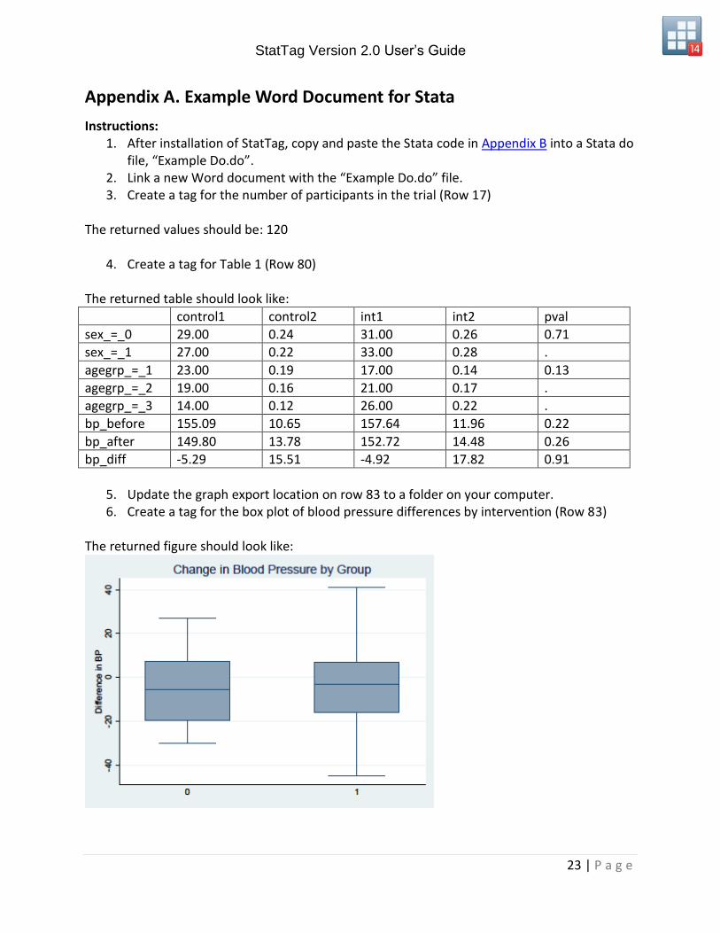
5. Update the graph export location on row 83 to a folder on your computer. 6. Create a tag for the box plot of blood pressure differences by intervention (Row 83)
The returned figure should look like:

StatTag Version 2.0 User’s Guide
24 | P a g e
Appendix B. Example Stata do file
* code to generate a Value, Matrix and Graph
* pull up the "bpwide" dataset that comes with Stata
sysuse bpwide
*generating additional variable,"intervention", through binomial distribution
random sampling with probability of ~0.5 to be assigned to intervention group
set seed 20151103
gen intervention=rbinomial(1,0.5)
label variable intervention "1=intervention 0=control"
*generate the difference in bp
gen bp_diff=bp_after-bp_before
label variable bp_diff "Difference in BP"
* get the number of observations on which we have no missing bp_before and
bp_after data
count if bp_before != . & bp_after != .
display r(N)
* variables to hold results
gen str12 rowname = ""
gen control1 = .
gen control2 = .
gen int1 = .
gen int2 = .
gen pval = .
* list of variables (one for categorical, one for continuous)
local catlist sex agegrp
local conlist bp_before bp_after bp_diff
* gen row counter
gen nn = _n
local rowct 1
* get total n
count if bp_before != . & bp_after != .
local totn = r(N)
* cycle through and fill out table 1
* note this is hard coded for intervention with 2 levels
* coded as 0 for control and 1 for intervention
foreach var of local catlist {
qui tabulate `var' intervention, chi2
replace pval = r(p) if nn == `rowct'
levelsof `var', local(varlevs)
foreach lev of local varlevs {
replace rowname = "`var' = `lev'" if nn == `rowct'
qui count if `var' == `lev' & intervention == 0
replace control1 = r(N) if nn == `rowct'
StatTag Version 2.0 User’s Guide
25 | P a g e
replace control2 = r(N)/`totn' if nn == `rowct'
qui count if `var'== `lev' & intervention == 1
replace int1 = r(N) if nn == `rowct'
replace int2 = r(N)/`totn' if nn == `rowct'
local rowct = `rowct' + 1
}
}
foreach var of local conlist {
replace rowname = "`var'" if nn == `rowct'
qui summarize `var' if intervention == 0
replace control1 = r(mean) if nn == `rowct'
replace control2 = r(sd) if nn == `rowct'
qui summarize `var' if intervention == 1
replace int1 = r(mean) if nn == `rowct'
replace int2 = r(sd) if nn == `rowct'
qui ttest `var', by(intervention)
replace pval = r(p) if nn == `rowct'
local rowct = `rowct' + 1
}
mkmat control1 - pval if nn < `rowct', matrix(tab1) rownames(rowname)
matrix list tab1
*comparing the change in bp by intervention group
graph box bp_diff, over(intervention) title("Change in Blood Pressure by
Group")
graph export "C:\Stata\BPDiff_BY_Intervention.pdf", as(pdf) replace
StatTag Version 2.0 User’s Guide
26 | P a g e
Appendix C. Example SAS sas file
*Run the following code to create the example dataset;
Data Example; Set SASUser.Drug; ID = _N_; Run;
Data Example;
Merge
Example (in=In1)
SASUser.BodyFat (rename=(Case=ID) IN=in2)
SASUser.NormTemp (in=In3);
by ID;
If IN1 and IN2 and In3;
Run;
*This dataset contains 130 observations and 26 variables;
Data Example; Set Example;
*Doses 1 and 2 are placebo, doses 3 and 4 are treated;
If DrugDose in (1,2) then Treatment = 0;
If DrugDose in (3,4) then Treatment = 1;
*Create Baseline BMI;
BaselineBMI = 703 * Weight / (Height * Height);
*Generate a small random number for change in BMI;
Random = ranuni(15) / 20;
PostBMI = BaselineBMI - (BaselineBMI * Random);
BMIChange = PostBMI - BaselineBMI;
Run;
*There is one person with implausibly high BMI due to data entry error;
Data Example; Set Example;
Where BaselineBMI <= 50;
Run;
*Count the number of observations in this dataset;
%let dsid=%sysfunc(open(Example));
%let num=%sysfunc(attrn(&dsid,nlobs));
%let rc=%sysfunc(close(&dsid));
%put #
*************************************************************
*** Table 1 ***
*************************************************************;
proc Freq data = Example; Table Treatment; Ods output onewayfreqs= groups;
Run;
data groups; set groups;
if Treatment = 0 then call
symput('Placebo',trim(left(put(Frequency,8.))));
if Treatment = 1 then call
symput('Treated',trim(left(put(Frequency,8.))));
Run;
%Put &Placebo;
%Put &Treated;
StatTag Version 2.0 User’s Guide
27 | P a g e
*The following builds a table 1 for a categorical input variable, including a
chi-squared p-value;
%Macro ByCategories(Data=,Var=,by=);
Proc Freq Data = &Data;
Table &by*&Var /chisq;
Ods Output CrossTabFreqs = Cat;
ods output chisq = Tests;
RUN;
Data Cat (Keep = &by N_PCT Level);
Set Cat;
Where (&by ^= . and ColPercent ^= .);
length N_PCT level $40.;
Level = trim(left(put(&Var,8.)));
N_PCT = trim(left(put(Frequency,8.0)))||"
("||trim(left(put(RowPercent,8.2)))||")";
Run;
Proc Sort Data = Cat; By Level; Run;
Proc Transpose Data = Cat Out = Cat;
Var N_PCT;
By Level;
Id &by;
Run;
Data Cat (Drop =_NAME_); Set Cat;
length variable type $40.;
variable = "%upcase(&var)";
type="N_PCT";
Run;
Data Tests; Set Tests;
If Statistic = "Chi-Square" then call
symput("pvalue",trim(left(put(prob,PVALUE6.4))));
Run;
Data Cat; Set Cat;
By Variable;
If First.variable then Pvalue = &Pvalue;
Run;
Proc Append Base = ByDescriptives Data = Cat Force; Run;
%Mend ByCategories;
*The following macro builds a table 1 for a continuous input variable
including either an ANOVA or Ttest p-value;
%Macro ByMeans(Data=,Var=,By=);
proc means data=&data mean stddev maxdec=2;
class &by;
var &var;
ods output Summary=cont;
run;
data cont (keep= &by Mean_SD);
set cont;
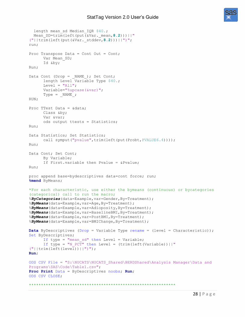
StatTag Version 2.0 User’s Guide
28 | P a g e
length mean_sd Median_IQR $40.;
Mean_SD=trim(left(put(&Var._mean,8.2)))||"
("||trim(left(put(&Var._stddev,8.2)))||")";
run;
Proc Transpose Data = Cont Out = Cont;
Var Mean_SD;
Id &by;
Run;
Data Cont (Drop = _NAME_); Set Cont;
length Level Variable Type $40.;
Level = "All";
Variable="%upcase(&var)";
Type = _NAME_;
RUN;
Proc TTest Data = &data;
Class &by;
Var &var;
ods output ttests = Statistics;
Run;
Data Statistics; Set Statistics;
call symput("pvalue",trim(left(put(Probt,PVALUE6.4))));
Run;
Data Cont; Set Cont;
By Variable;
If First.variable then Pvalue = &Pvalue;
Run;
proc append base=bydescriptives data=cont force; run;
%mend ByMeans;
*For each characteristic, use either the bymeans (continuous) or bycategories
(categorical) call to run the macro;
%ByCategories(data=Example,var=Gender,By=Treatment);
%ByMeans(data=Example,var=Age,By=Treatment);
%ByMeans(data=Example,var=Adioposity,By=Treatment);
%ByMeans(data=Example,var=BaselineBMI,By=Treatment);
%ByMeans(data=Example,var=PostBMI,By=Treatment);
%ByMeans(data=Example,var=BMIChange,By=Treatment);
Data ByDescriptives (Drop = Variable Type rename = (level = Characteristic));
Set ByDescriptives;
If type = "mean_sd" then Level = Variable;
If type = "N_PCT" then Level = (trim(left(Variable))||"
("||trim(left(level))||")");
Run;
ODS CSV File = "S:\NUCATS\NUCATS_Shared\BERDShared\Analysis Manager\Data and
Programs\SAS\Code\Table1.csv";
Proc Print Data = ByDescriptives noobs; Run;
ODS CSV CLOSE;
*************************************************************
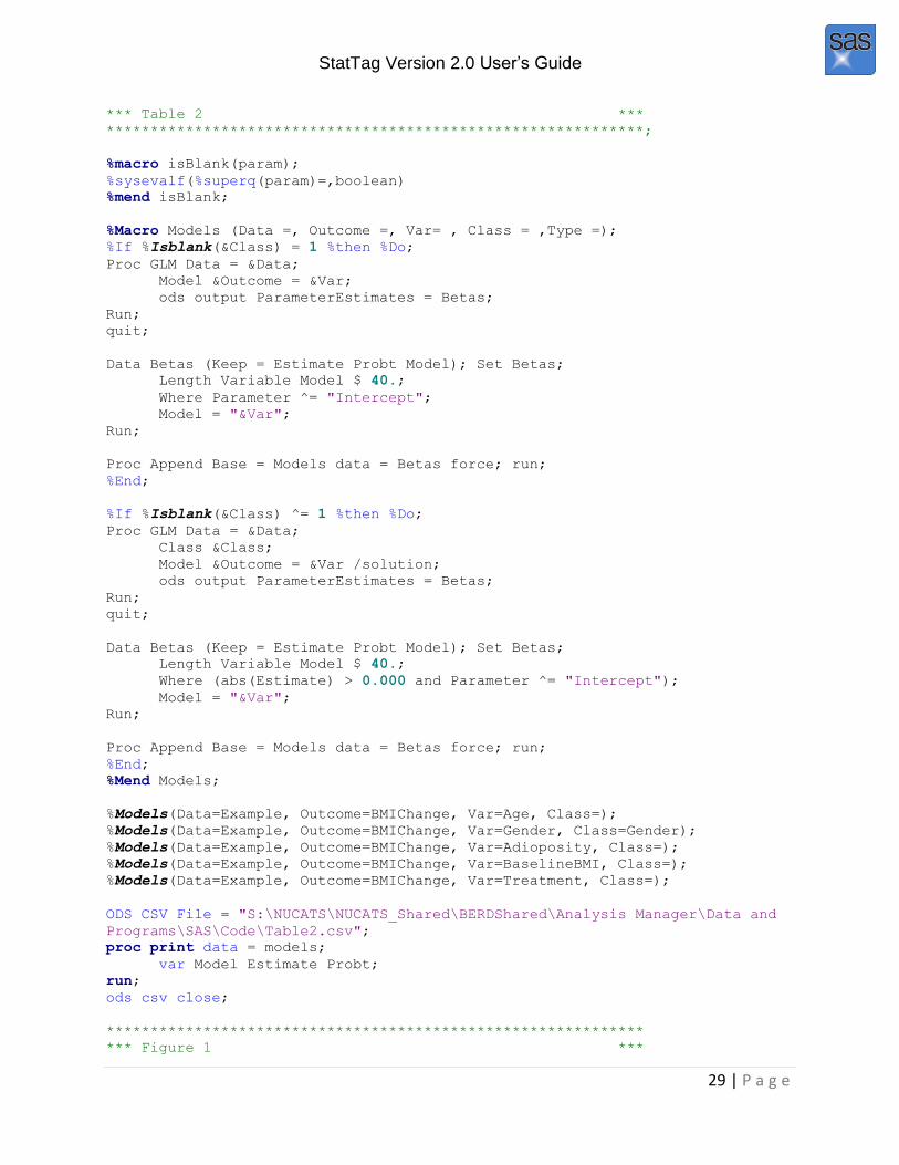
StatTag Version 2.0 User’s Guide
29 | P a g e
*** Table 2 ***
*************************************************************;
%macro isBlank(param);
%sysevalf(%superq(param)=,boolean) %mend isBlank;
%Macro Models (Data =, Outcome =, Var= , Class = ,Type =);
%If %Isblank(&Class) = 1 %then %Do;
Proc GLM Data = &Data;
Model &Outcome = &Var;
ods output ParameterEstimates = Betas;
Run;
quit;
Data Betas (Keep = Estimate Probt Model); Set Betas;
Length Variable Model $ 40.;
Where Parameter ^= "Intercept";
Model = "&Var";
Run;
Proc Append Base = Models data = Betas force; run;
%End;
%If %Isblank(&Class) ^= 1 %then %Do;
Proc GLM Data = &Data;
Class &Class;
Model &Outcome = &Var /solution;
ods output ParameterEstimates = Betas;
Run;
quit;
Data Betas (Keep = Estimate Probt Model); Set Betas;
Length Variable Model $ 40.;
Where (abs(Estimate) > 0.000 and Parameter ^= "Intercept");
Model = "&Var";
Run;
Proc Append Base = Models data = Betas force; run;
%End;
%Mend Models;
%Models(Data=Example, Outcome=BMIChange, Var=Age, Class=);
%Models(Data=Example, Outcome=BMIChange, Var=Gender, Class=Gender);
%Models(Data=Example, Outcome=BMIChange, Var=Adioposity, Class=);
%Models(Data=Example, Outcome=BMIChange, Var=BaselineBMI, Class=);
%Models(Data=Example, Outcome=BMIChange, Var=Treatment, Class=);
ODS CSV File = "S:\NUCATS\NUCATS_Shared\BERDShared\Analysis Manager\Data and
Programs\SAS\Code\Table2.csv";
proc print data = models;
var Model Estimate Probt;
run;
ods csv close;
*************************************************************
*** Figure 1 ***
StatTag Version 2.0 User’s Guide
30 | P a g e
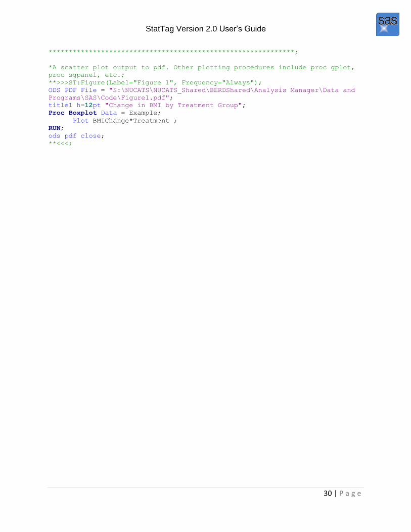
*************************************************************;
*A scatter plot output to pdf. Other plotting procedures include proc gplot,
proc sgpanel, etc.;
**>>>ST:Figure(Label="Figure 1", Frequency="Always");
ODS PDF File = "S:\NUCATS\NUCATS_Shared\BERDShared\Analysis Manager\Data and
Programs\SAS\Code\Figure1.pdf";
title1 h=12pt "Change in BMI by Treatment Group";
Proc Boxplot Data = Example;
Plot BMIChange*Treatment ; RUN;
ods pdf close;
**<<<;
StatTag Version 2.0 User’s Guide
31 | P a g e
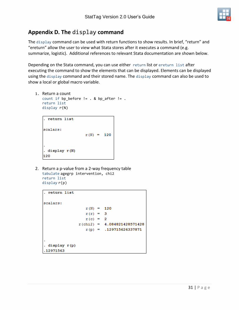
Appendix D. The display command
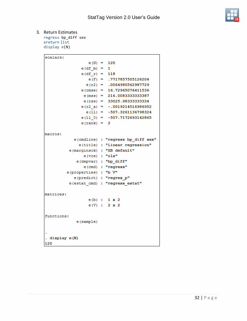
The display command can be used with return functions to show results. In brief, “return” and “ereturn” allow the user to view what Stata stores after it executes a command (e.g. summarize, logistic). Additional references to relevant Stata documentation are shown below. Depending on the Stata command, you can use either return list or ereturn list after executing the command to show the elements that can be displayed. Elements can be displayed using the display command and their stored name. The display command can also be used to show a local or global macro variable.
1. Return a count count if bp_before != . & bp_after != . return list display r(N)
2. Return a p-value from a 2-way frequency table tabulate agegrp intervention, chi2 return list display r(p)
StatTag Version 2.0 User’s Guide
32 | P a g e
3. Return Estimates regress bp_diff sex ereturn list display e(N)
StatTag Version 2.0 User’s Guide
33 | P a g e
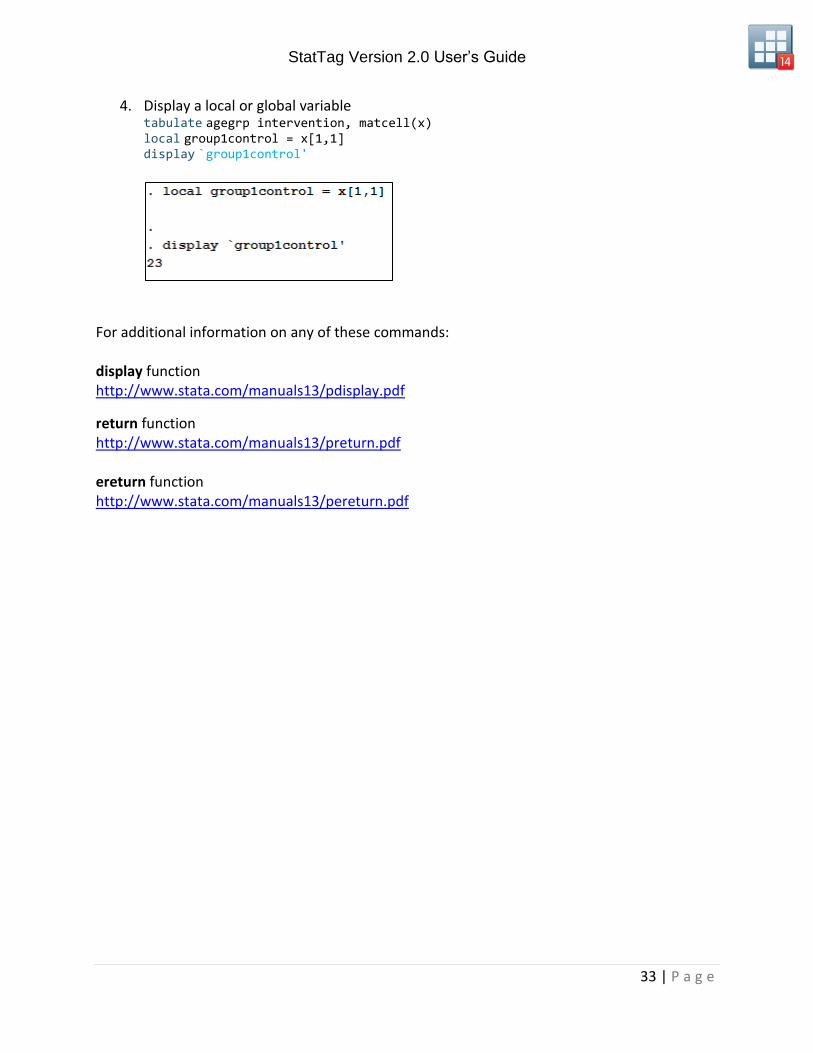
4. Display a local or global variable tabulate agegrp intervention, matcell(x) local group1control = x[1,1] display `group1control'
For additional information on any of these commands: display function http://www.stata.com/manuals13/pdisplay.pdf
return function http://www.stata.com/manuals13/preturn.pdf ereturn function http://www.stata.com/manuals13/pereturn.pdf
StatTag Version 2.0 User’s Guide
34 | P a g e
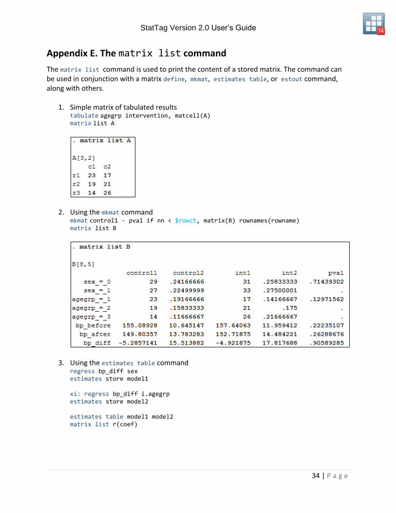
Appendix E. The matrix list command
The matrix list command is used to print the content of a stored matrix. The command can be used in conjunction with a matrix define, mkmat, estimates table, or estout command, along with others.
1. Simple matrix of tabulated results tabulate agegrp intervention, matcell(A) matrix list A
2. Using the mkmat command mkmat control1 - pval if nn < $rowct, matrix(B) rownames(rowname) matrix list B
3. Using the estimates table command regress bp_diff sex estimates store model1 xi: regress bp_diff i.agegrp estimates store model2
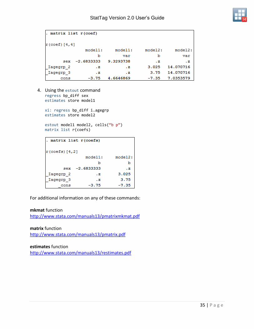
estimates table model1 model2 matrix list r(coef)
StatTag Version 2.0 User’s Guide
35 | P a g e
4. Using the estout command regress bp_diff sex estimates store model1 xi: regress bp_diff i.agegrp estimates store model2
estout model1 model2, cells(“b p”) matrix list r(coefs)
For additional information on any of these commands: mkmat function http://www.stata.com/manuals13/pmatrixmkmat.pdf matrix function http://www.stata.com/manuals13/pmatrix.pdf estimates function http://www.stata.com/manuals13/restimates.pdf
StatTag Version 2.0 User’s Guide
36 | P a g e
Appendix F. The graph export command
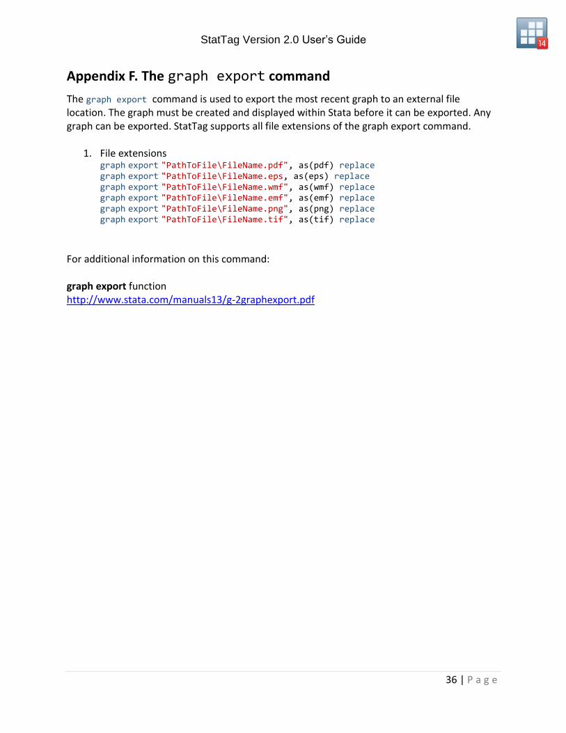
The graph export command is used to export the most recent graph to an external file location. The graph must be created and displayed within Stata before it can be exported. Any graph can be exported. StatTag supports all file extensions of the graph export command.
1. File extensions graph export "PathToFile\FileName.pdf", as(pdf) replace graph export "PathToFile\FileName.eps, as(eps) replace graph export "PathToFile\FileName.wmf", as(wmf) replace graph export "PathToFile\FileName.emf", as(emf) replace graph export "PathToFile\FileName.png", as(png) replace graph export "PathToFile\FileName.tif", as(tif) replace
For additional information on this command: graph export function http://www.stata.com/manuals13/g-2graphexport.pdf
StatTag Version 2.0 User’s Guide
37 | P a g e
Appendix G. The %put command
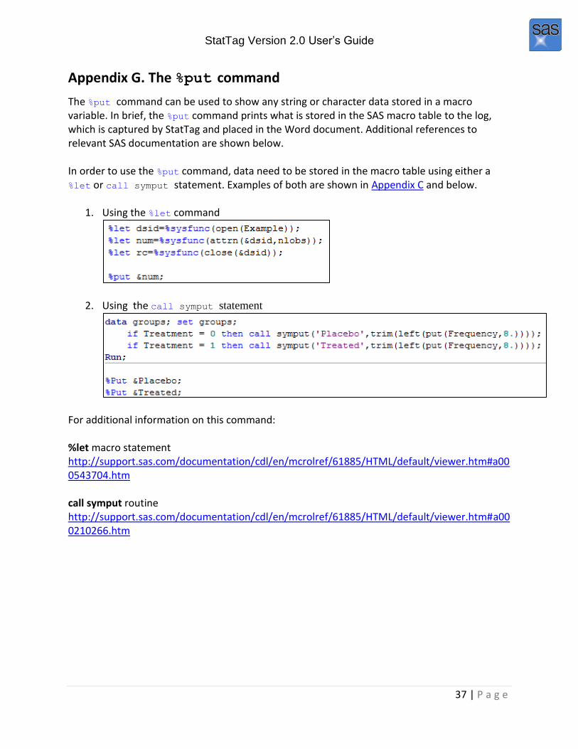
The %put command can be used to show any string or character data stored in a macro variable. In brief, the %put command prints what is stored in the SAS macro table to the log, which is captured by StatTag and placed in the Word document. Additional references to relevant SAS documentation are shown below. In order to use the %put command, data need to be stored in the macro table using either a %let or call symput statement. Examples of both are shown in Appendix C and below.
1. Using the %let command
2. Using the call symput statement
For additional information on this command: %let macro statement http://support.sas.com/documentation/cdl/en/mcrolref/61885/HTML/default/viewer.htm#a000543704.htm call symput routine http://support.sas.com/documentation/cdl/en/mcrolref/61885/HTML/default/viewer.htm#a000210266.htm
StatTag Version 2.0 User’s Guide
38 | P a g e
Appendix H. The ODS CSV and ODS PDF commands
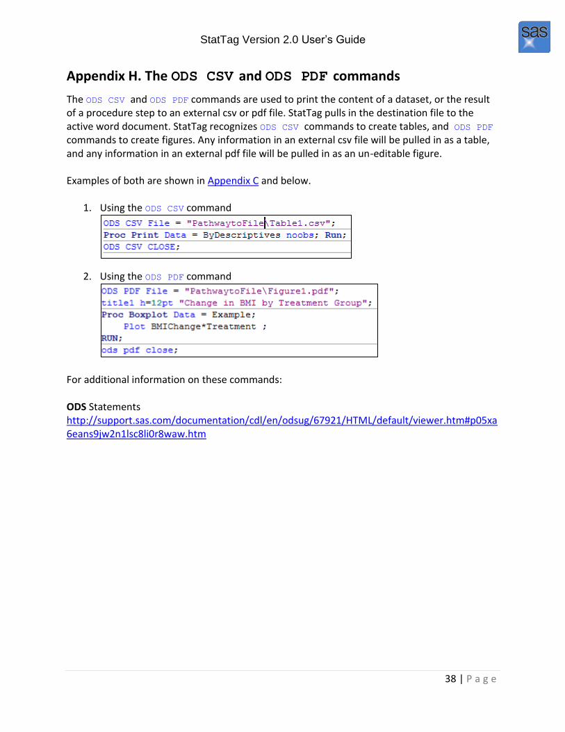
The ODS CSV and ODS PDF commands are used to print the content of a dataset, or the result of a procedure step to an external csv or pdf file. StatTag pulls in the destination file to the active word document. StatTag recognizes ODS CSV commands to create tables, and ODS PDF commands to create figures. Any information in an external csv file will be pulled in as a table, and any information in an external pdf file will be pulled in as an un-editable figure. Examples of both are shown in Appendix C and below.
1. Using the ODS CSV command
2. Using the ODS PDF command
For additional information on these commands: ODS Statements http://support.sas.com/documentation/cdl/en/odsug/67921/HTML/default/viewer.htm#p05xa6eans9jw2n1lsc8li0r8waw.htm

StatTag Version 2.0 User’s Guide
39 | P a g e
Appendix I. Licenses
License for StatTag
The MIT License (MIT) Copyright (c) 2016, Northwestern University, All Rights Reserved Permission is hereby granted, free of charge, to any person obtaining a copy of this software and associated documentation files (the "Software"), to deal in the Software without restriction, including without limitation the rights to use, copy, modify, merge, publish, distribute, sublicense, and/or sell copies of the Software, and to permit persons to whom the Software is furnished to do so, subject to the following conditions: The above copyright notice and this permission notice shall be included in all copies or substantial portions of the Software. THE SOFTWARE IS PROVIDED "AS IS", WITHOUT WARRANTY OF ANY KIND, EXPRESS OR IMPLIED, INCLUDING BUT NOT LIMITED TO THE WARRANTIES OF MERCHANTABILITY, FITNESS FOR A PARTICULAR PURPOSE AND NONINFRINGEMENT. IN NO EVENT SHALL THE AUTHORS OR COPYRIGHT HOLDERS BE LIABLE FOR ANY CLAIM, DAMAGES OR OTHER LIABILITY, WHETHER IN AN ACTION OF CONTRACT, TORT OR OTHERWISE, ARISING FROM, OUT OF OR IN CONNECTION WITH THE SOFTWARE OR THE USE OR OTHER DEALINGS IN THE SOFTWARE.
License for Scintilla and SciTE
License for Scintilla and SciTE Copyright 1998-2003 by Neil Hodgson [email protected], All Rights Reserved Permission to use, copy, modify, and distribute this software and its documentation for any purpose and without fee is hereby granted, provided that the above copyright notice appear in all copies and that both that copyright notice and this permission notice appear in supporting documentation. NEIL HODGSON DISCLAIMS ALL WARRANTIES WITH REGARD TO THIS SOFTWARE, INCLUDING ALL IMPLIED WARRANTIES OF MERCHANTABILITY AND FITNESS, IN NO EVENT SHALL NEIL HODGSON BE LIABLE FOR ANY SPECIAL, INDIRECT OR CONSEQUENTIAL DAMAGES OR ANY DAMAGES WHATSOEVER RESULTING FROM LOSS OF USE, DATA OR PROFITS, WHETHER IN AN ACTION OF CONTRACT, NEGLIGENCE OR OTHER TORTIOUS ACTION, ARISING OUT OF OR IN CONNECTION WITH THE USE OR PERFORMANCE OF THIS SOFTWARE.
StatTag Version 2.0 User’s Guide
40 | P a g e
License for ScintillaNET
The MIT License (MIT) Copyright (c) 2016, Jacob Slusser, https://github.com/jacobslusser Permission is hereby granted, free of charge, to any person obtaining a copy of this software and associated documentation files (the "Software"), to deal in the Software without restriction, including without limitation the rights to use, copy, modify, merge, publish, distribute, sublicense, and/or sell copies of the Software, and to permit persons to whom the Software is furnished to do so, subject to the following conditions: The above copyright notice and this permission notice shall be included in all copies or substantial portions of the Software. THE SOFTWARE IS PROVIDED "AS IS", WITHOUT WARRANTY OF ANY KIND, EXPRESS OR IMPLIED, INCLUDING BUT NOT LIMITED TO THE WARRANTIES OF MERCHANTABILITY, FITNESS FOR A PARTICULAR PURPOSE AND NONINFRINGEMENT. IN NO EVENT SHALL THE AUTHORS OR COPYRIGHT HOLDERS BE LIABLE FOR ANY CLAIM, DAMAGES OR OTHER LIABILITY, WHETHER IN AN ACTION OF CONTRACT, TORT OR OTHERWISE, ARISING FROM, OUT OF OR IN CONNECTION WITH THE SOFTWARE OR THE USE OR OTHER DEALINGS IN THE SOFTWARE.
License for Json.NET
The MIT License (MIT) Copyright (c) 2007 James Newton-King Permission is hereby granted, free of charge, to any person obtaining a copy of this software and associated documentation files (the "Software"), to deal in the Software without restriction, including without limitation the rights to use, copy, modify, merge, publish, distribute, sublicense, and/or sell copies of the Software, and to permit persons to whom the Software is furnished to do so, subject to the following conditions: The above copyright notice and this permission notice shall be included in all copies or substantial portions of the Software. THE SOFTWARE IS PROVIDED "AS IS", WITHOUT WARRANTY OF ANY KIND, EXPRESS OR IMPLIED, INCLUDING BUT NOT LIMITED TO THE WARRANTIES OF MERCHANTABILITY, FITNESS FOR A PARTICULAR PURPOSE AND NONINFRINGEMENT. IN NO EVENT SHALL THE AUTHORS OR COPYRIGHT HOLDERS BE LIABLE FOR ANY CLAIM, DAMAGES OR OTHER LIABILITY, WHETHER IN AN ACTION OF CONTRACT, TORT OR OTHERWISE, ARISING FROM, OUT OF OR IN CONNECTION WITH THE SOFTWARE OR THE USE OR OTHER DEALINGS IN THE SOFTWARE.