Example 1 (knnl917.sas)
45
Example 1 (knnl917.sas) Y = months survival Treatment (3 levels)
-
Upload
joseph-garrison -
Category
Documents
-
view
30 -
download
2
description
Example 1 (knnl917.sas). Y = months survival Treatment (3 levels). Example 1: ANOVA. Example 1: Including the covariate. Example 1: ANCOVA. Example 1: ANCOVA (cont). Example 1: ANCOVA comparison. Example 2. Y = months survival Treatment (3 levels). Example 2: ANOVA. - PowerPoint PPT Presentation
Transcript of Example 1 (knnl917.sas)
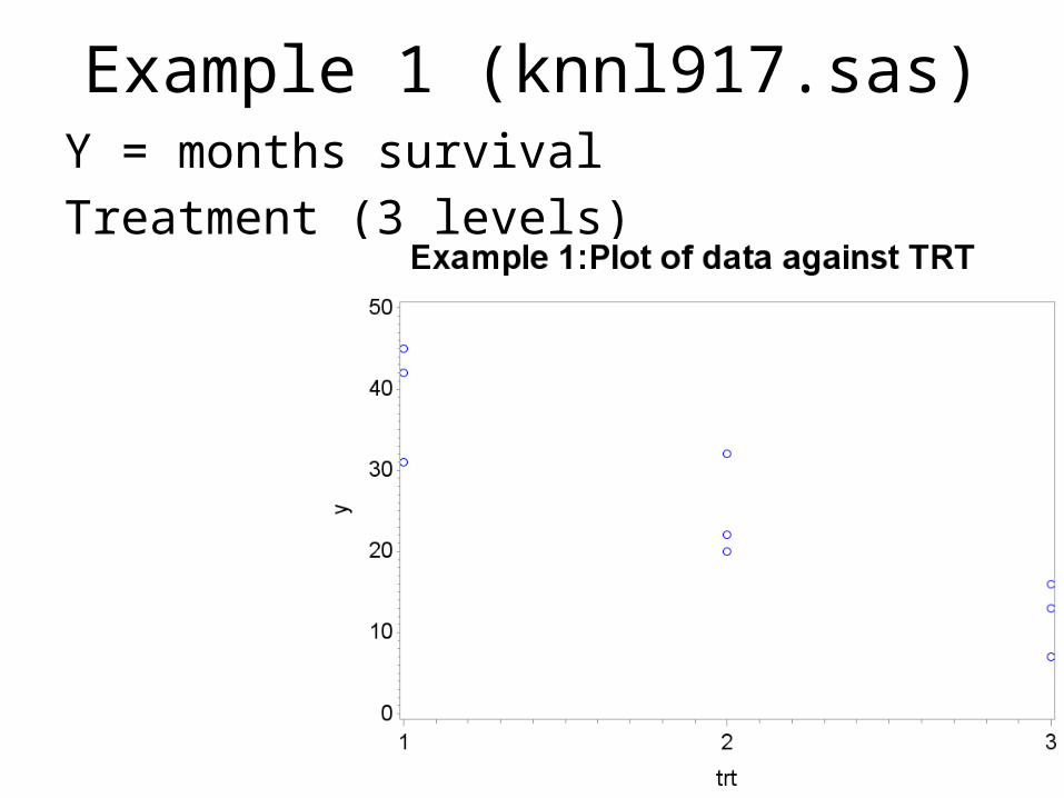
Example 1 (knnl917.sas)Y = months survivalTreatment (3 levels)

Example 1: ANOVASource DF Sum of Squares
Mean Square
F Value Pr > F
Model 2 1122.666667 561.333333 14.43 0.0051Error 6 233.333333 38.888889Corrected Total 8 1356.000000
Means with the same letterare not significantly different.Tukey Grouping Mean N trt
A 39.333 3 1A
B A 24.667 3 2BB 12.000 3 3
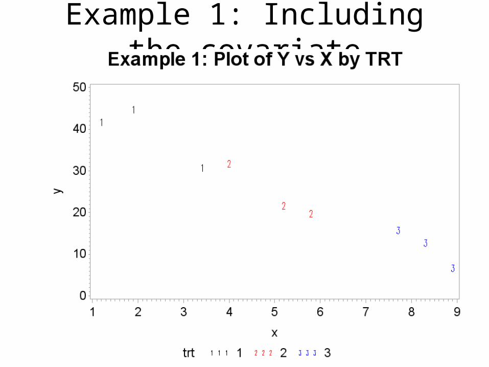
Example 1: Including the covariate
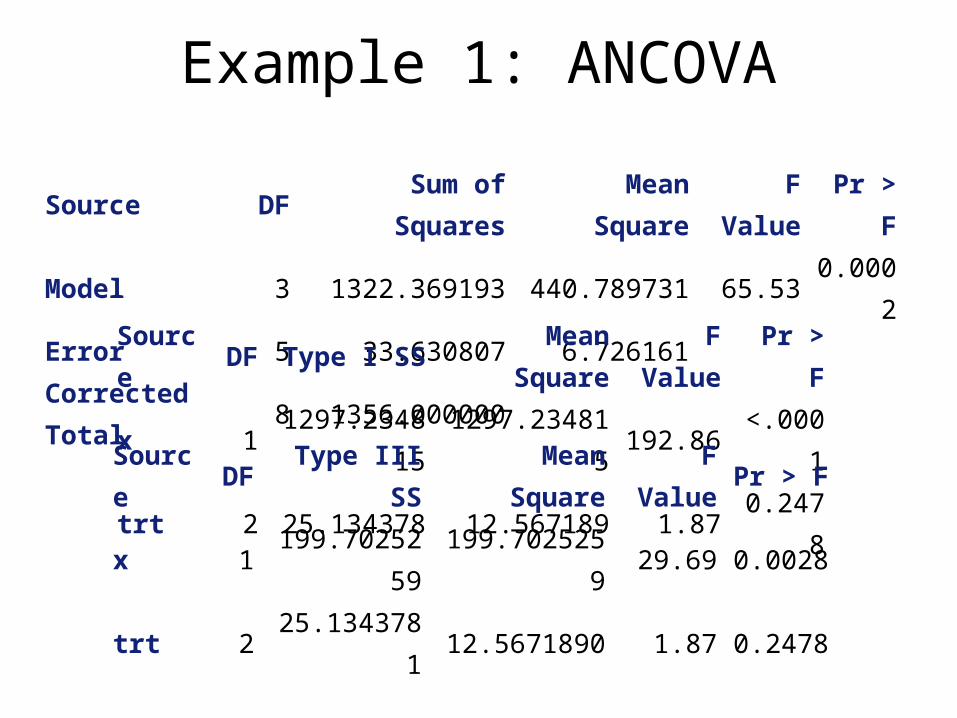
Example 1: ANCOVA
Source DF Sum of Squares Mean Square F Value Pr > FModel 3 1322.369193 440.789731 65.53 0.0002Error 5 33.630807 6.726161Corrected Total 8 1356.000000
Source DF Type I SS Mean Square F Value Pr > Fx 1 1297.234815 1297.234815 192.86 <.0001trt 2 25.134378 12.567189 1.87 0.2478
Source DF Type III SS Mean Square F Value Pr > Fx 1 199.7025259 199.7025259 29.69 0.0028trt 2 25.1343781 12.5671890 1.87 0.2478
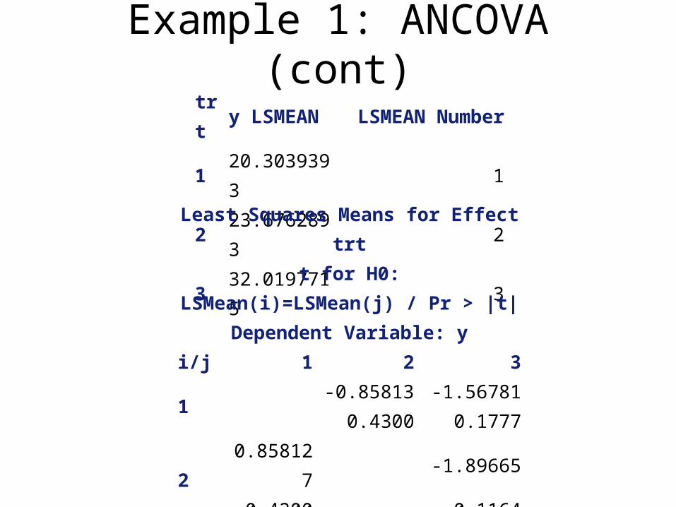
Example 1: ANCOVA (cont)trt y LSMEAN LSMEAN Number1 20.3039393 12 23.6762893 23 32.0197715 3
Least Squares Means for Effect trtt for H0: LSMean(i)=LSMean(j) / Pr > |t|
Dependent Variable: yi/j 1 2 3
1-0.85813 -1.56781
0.4300 0.1777
20.858127 -1.89665
0.4300 0.1164
31.567807 1.89665
0.1777 0.1164
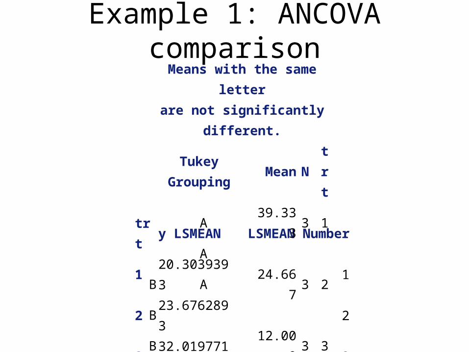
Example 1: ANCOVA comparison
trt y LSMEAN LSMEAN Number1 20.3039393 12 23.6762893 23 32.0197715 3
Means with the same letterare not significantly different.Tukey Grouping Mean N trt
A 39.333 3 1A
B A 24.667 3 2BB 12.000 3 3

Example 2Y = months survivalTreatment (3 levels)
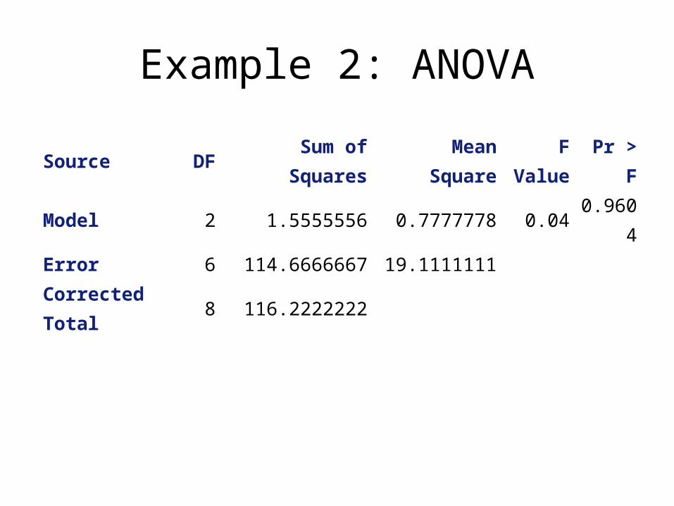
Example 2: ANOVA
Source DF Sum of Squares Mean Square F Value Pr > FModel 2 1.5555556 0.7777778 0.04 0.9604Error 6 114.6666667 19.1111111Corrected Total 8 116.2222222
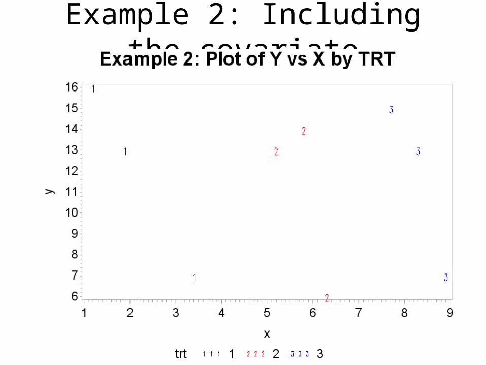
Example 2: Including the covariate
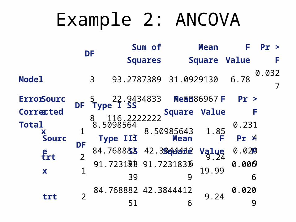
Example 2: ANCOVADF Sum of Squares Mean Square F Value Pr > F
Model 3 93.2787389 31.0929130 6.78 0.0327Error 5 22.9434833 4.5886967Corrected Total 8 116.2222222
Source DF Type I SS Mean Square F Value Pr > Fx 1 8.50985643 8.50985643 1.85 0.2314trt 2 84.76888251 42.38444126 9.24 0.0209
Source DF Type III SSMean
SquareF Value Pr > F
x 1 91.72318339 91.72318339 19.99 0.0066trt 2 84.76888251 42.38444126 9.24 0.0209
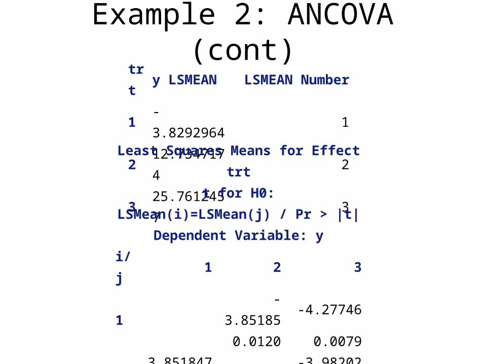
Example 2: ANCOVA (cont)trt y LSMEAN LSMEAN Number1 -3.8292964 12 12.7347174 23 25.7612457 3
Least Squares Means for Effect trtt for H0: LSMean(i)=LSMean(j) / Pr > |t|
Dependent Variable: yi/j 1 2 3
1-3.85185 -4.27746
0.0120 0.0079
23.851847 -3.98202
0.0120 0.0105
34.277456 3.982016
0.0079 0.0105
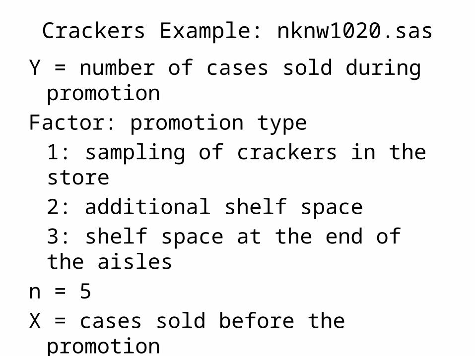
Crackers Example: nknw1020.sasY = number of cases sold during promotionFactor: promotion type
1: sampling of crackers in the store2: additional shelf space3: shelf space at the end of the aisles
n = 5X = cases sold before the promotion
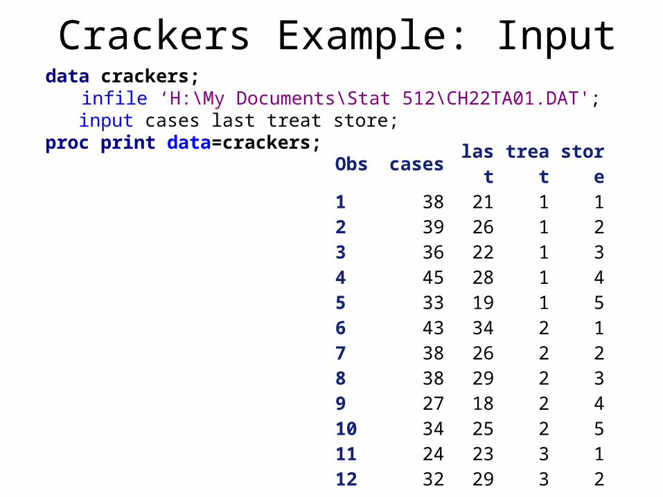
Crackers Example: Inputdata crackers;
infile ‘H:\My Documents\Stat 512\CH22TA01.DAT'; input cases last treat store;proc print data=crackers; Obs cases last treat store
1 38 21 1 12 39 26 1 23 36 22 1 34 45 28 1 45 33 19 1 56 43 34 2 17 38 26 2 28 38 29 2 39 27 18 2 410 34 25 2 511 24 23 3 112 32 29 3 213 31 30 3 314 21 16 3 415 28 29 3 5
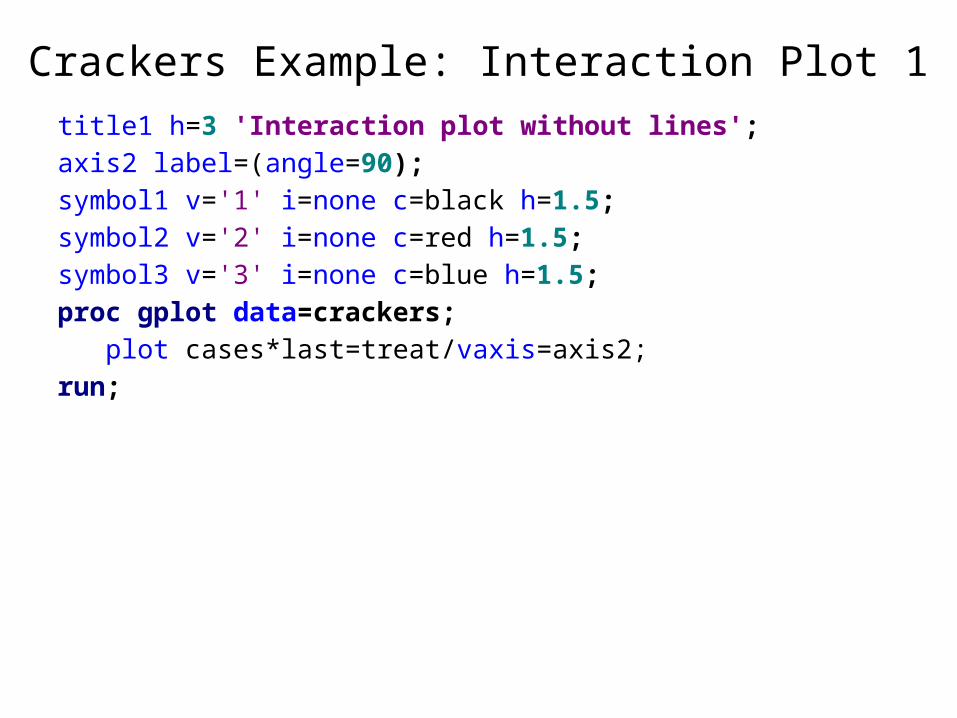
Crackers Example: Interaction Plot 1title1 h=3 'Interaction plot without lines';axis2 label=(angle=90);symbol1 v='1' i=none c=black h=1.5;symbol2 v='2' i=none c=red h=1.5;symbol3 v='3' i=none c=blue h=1.5;proc gplot data=crackers; plot cases*last=treat/vaxis=axis2;run;
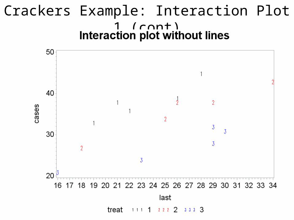
Crackers Example: Interaction Plot 1 (cont)
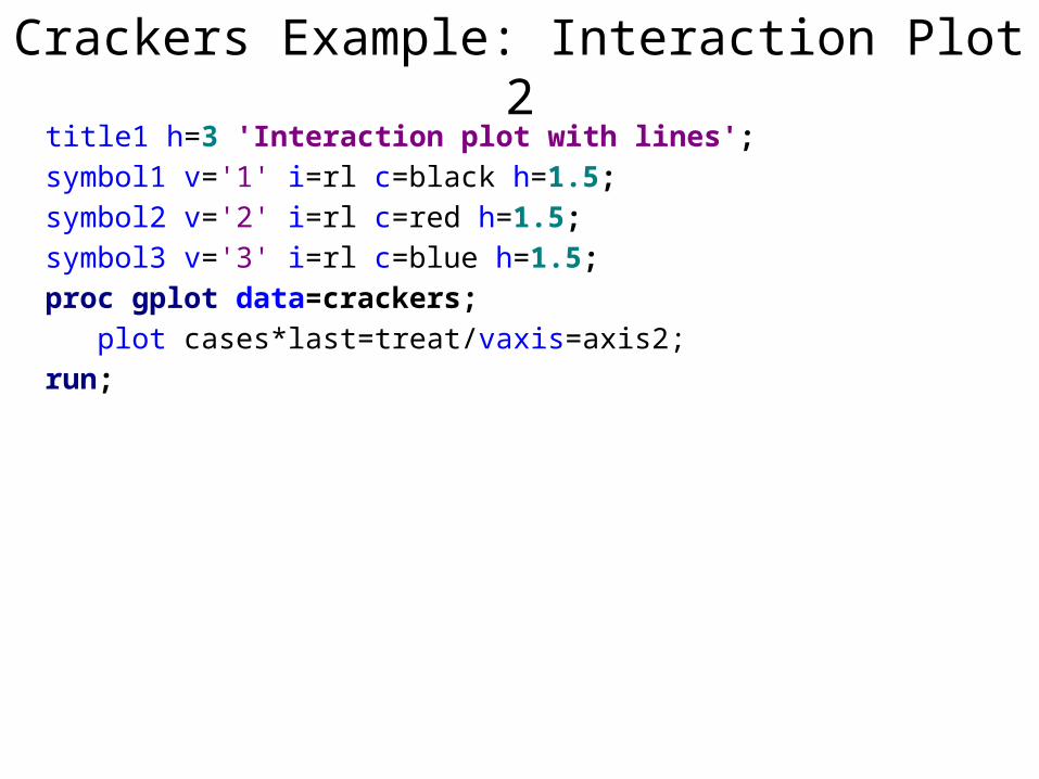
Crackers Example: Interaction Plot 2title1 h=3 'Interaction plot with lines';symbol1 v='1' i=rl c=black h=1.5;symbol2 v='2' i=rl c=red h=1.5;symbol3 v='3' i=rl c=blue h=1.5;proc gplot data=crackers; plot cases*last=treat/vaxis=axis2;run;
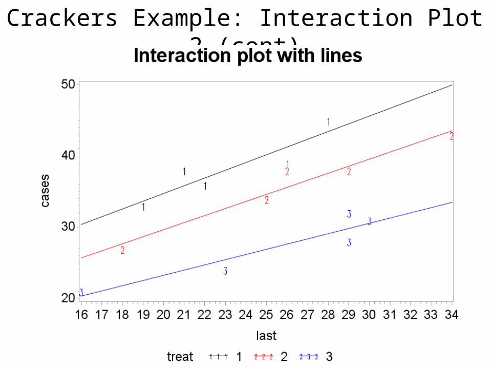
Crackers Example: Interaction Plot 2 (cont)
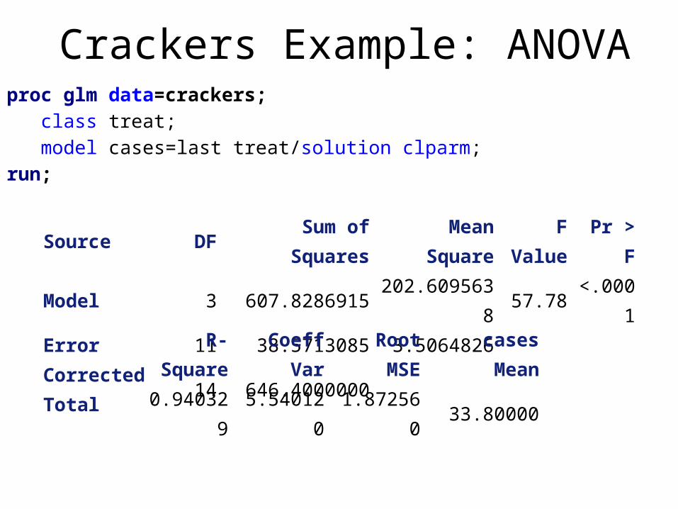
Crackers Example: ANOVAproc glm data=crackers; class treat; model cases=last treat/solution clparm;run;
Source DF Sum of SquaresMean
SquareF Value Pr > F
Model 3 607.8286915 202.6095638 57.78 <.0001Error 11 38.5713085 3.5064826Corrected Total 14 646.4000000
R-Square Coeff VarRoot MSE
cases Mean
0.940329 5.540120 1.872560 33.80000

Crackers Example: ANOVA (cont)Source DF Type I SS Mean Square F Value Pr > Flast 1 190.6777778 190.6777778 54.38 <.0001treat 2 417.1509137 208.5754568 59.48 <.0001
Source DF Type III SSMean
SquareF Value Pr > F
last 1 269.0286915 269.0286915 76.72 <.0001treat 2 417.1509137 208.5754568 59.48 <.0001
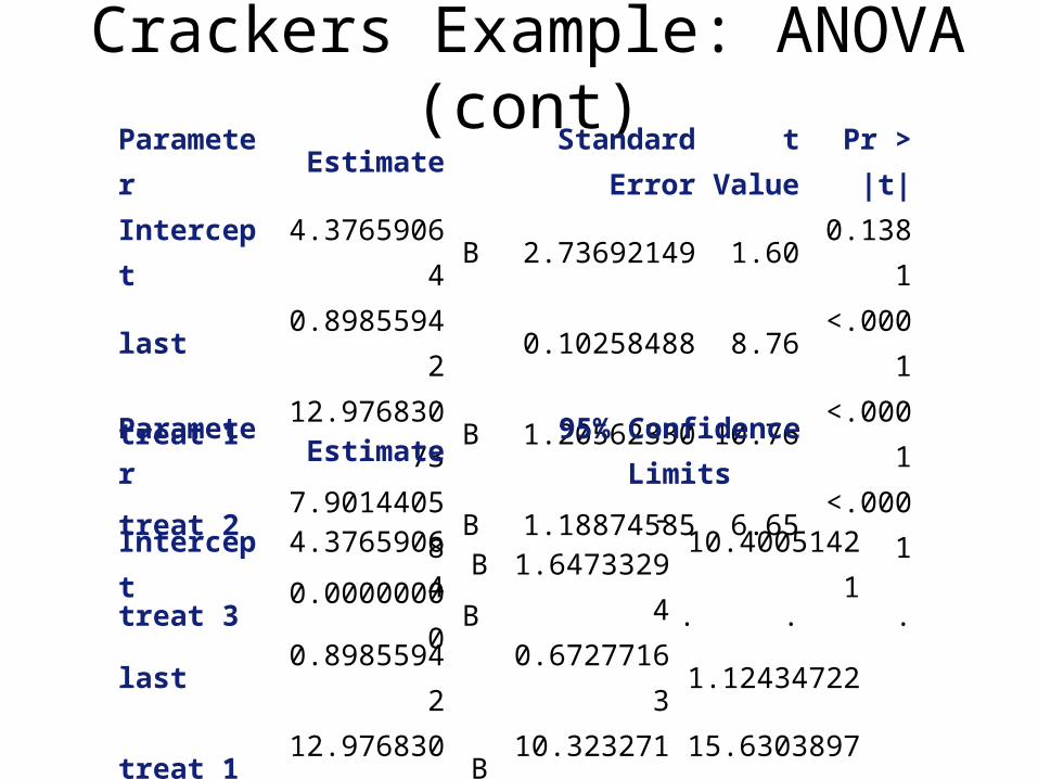
Crackers Example: ANOVA (cont)Parameter Estimate Standard Error
t Value
Pr > |t|
Intercept 4.37659064 B 2.73692149 1.60 0.1381last 0.89855942 0.10258488 8.76 <.0001treat 1 12.97683073 B 1.20562330 10.76 <.0001treat 2 7.90144058 B 1.18874585 6.65 <.0001treat 3 0.00000000 B . . .
Parameter Estimate 95% Confidence LimitsIntercept 4.37659064 B -1.64733294 10.40051421last 0.89855942 0.67277163 1.12434722treat 1 12.97683073 B 10.32327174 15.63038972treat 2 7.90144058 B 5.28502860 10.51785255treat 3 0.00000000 B . .
Crackers Example: LSMEANSproc glm data=crackers; class treat; model cases=last treat; lsmeans treat/stderr tdiff pdiff cl;run;
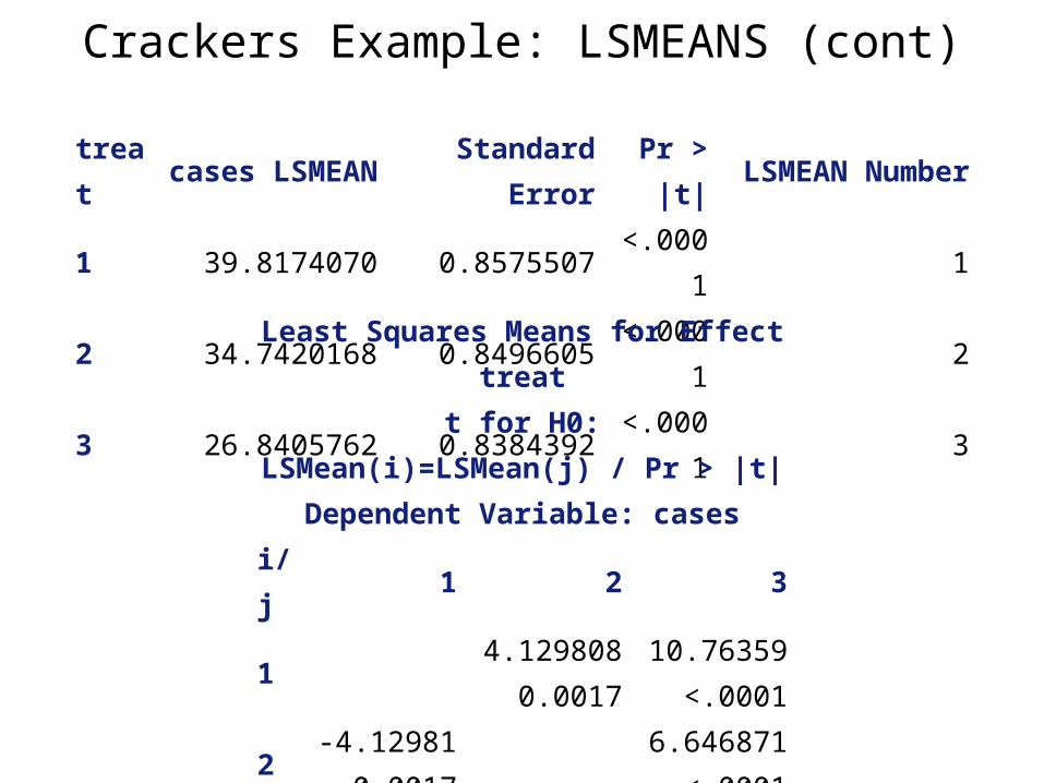
Crackers Example: LSMEANS (cont)
treat cases LSMEAN Standard Error Pr > |t| LSMEAN Number1 39.8174070 0.8575507 <.0001 12 34.7420168 0.8496605 <.0001 23 26.8405762 0.8384392 <.0001 3
Least Squares Means for Effect treatt for H0: LSMean(i)=LSMean(j) / Pr > |t|
Dependent Variable: casesi/j 1 2 3
14.129808 10.76359
0.0017 <.0001
2-4.12981 6.646871
0.0017 <.0001
3-10.7636 -6.64687
<.0001 <.0001
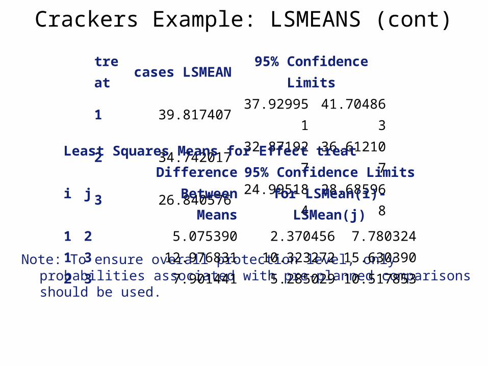
Crackers Example: LSMEANS (cont)
Note: To ensure overall protection level, only probabilities associated with pre-planned comparisons should be used.
treat cases LSMEAN 95% Confidence Limits1 39.817407 37.929951 41.7048632 34.742017 32.871927 36.6121073 26.840576 24.995184 28.685968
Least Squares Means for Effect treat
i jDifference Between
Means95% Confidence Limits for
LSMean(i)-LSMean(j)1 2 5.075390 2.370456 7.7803241 3 12.976831 10.323272 15.6303902 3 7.901441 5.285029 10.517853
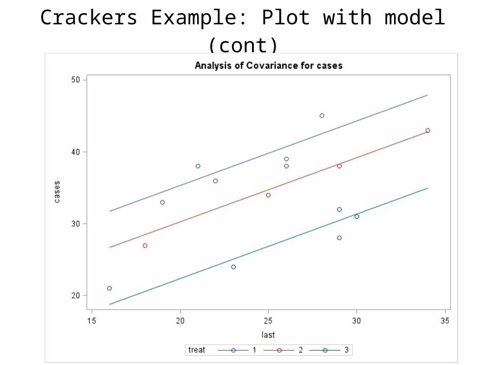
Crackers Example: Plot with model (cont)
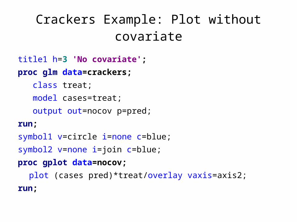
Crackers Example: Plot without covariate
title1 h=3 'No covariate';proc glm data=crackers; class treat; model cases=treat; output out=nocov p=pred;run;symbol1 v=circle i=none c=blue;symbol2 v=none i=join c=blue;proc gplot data=nocov;
plot (cases pred)*treat/overlay vaxis=axis2;run;
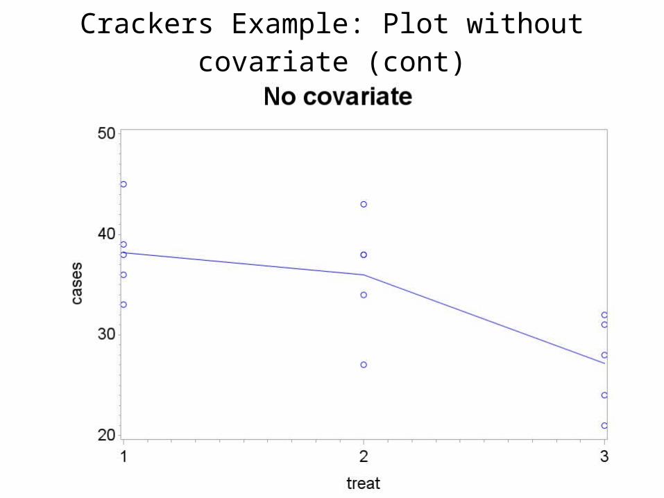
Crackers Example: Plot without covariate (cont)
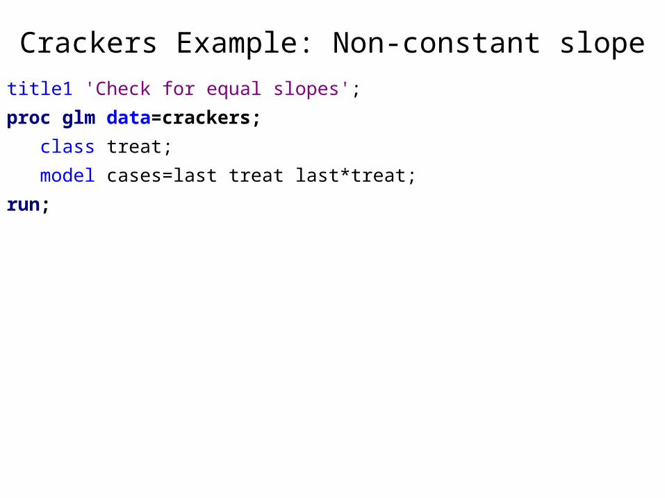
Crackers Example: Non-constant slopetitle1 'Check for equal slopes';proc glm data=crackers; class treat; model cases=last treat last*treat;run;
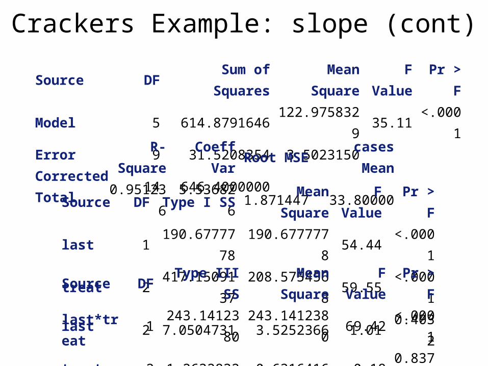
Crackers Example: slope (cont)
Source DF Sum of SquaresMean
SquareF Value Pr > F
Model 5 614.8791646 122.9758329 35.11 <.0001Error 9 31.5208354 3.5023150Corrected Total 14 646.4000000
R-Square Coeff Var Root MSE cases Mean0.951236 5.536826 1.871447 33.80000
Source DF Type I SS Mean Square F Value Pr > Flast 1 190.6777778 190.6777778 54.44 <.0001treat 2 417.1509137 208.5754568 59.55 <.0001last*treat 2 7.0504731 3.5252366 1.01 0.4032
Source DF Type III SSMean
SquareF Value Pr > F
last 1 243.1412380 243.1412380 69.42 <.0001treat 2 1.2632832 0.6316416 0.18 0.8379last*treat 2 7.0504731 3.5252366 1.01 0.4032
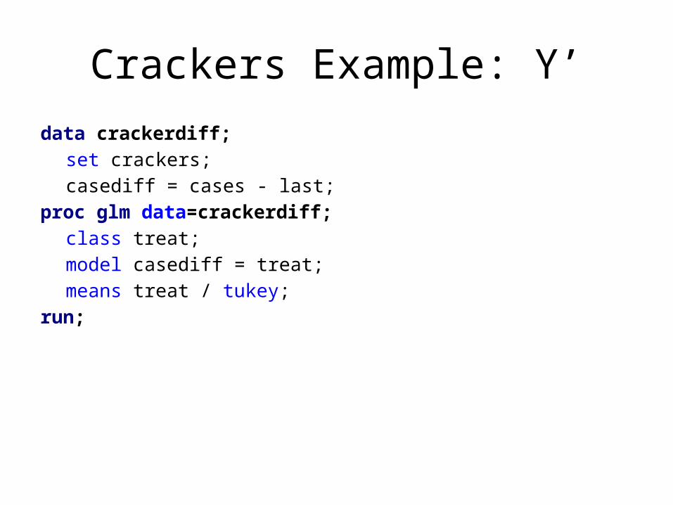
Crackers Example: Y’data crackerdiff;
set crackers;casediff = cases - last;
proc glm data=crackerdiff;class treat;model casediff = treat;means treat / tukey;
run;
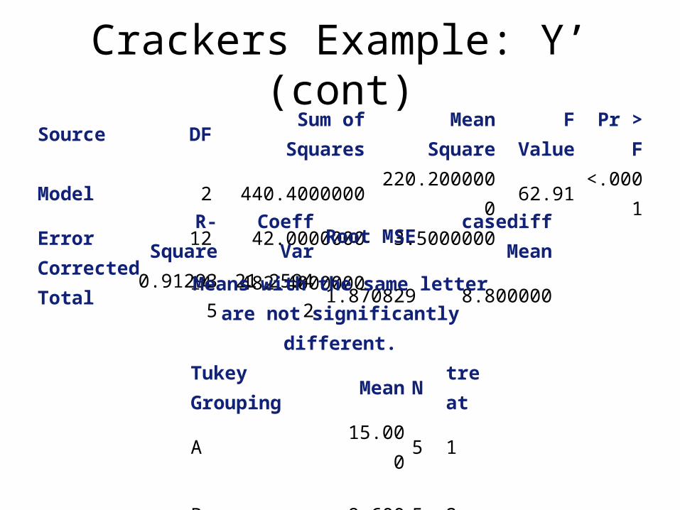
Crackers Example: Y’ (cont)Source DF Sum of Squares Mean Square F Value Pr > FModel 2 440.4000000 220.2000000 62.91 <.0001Error 12 42.0000000 3.5000000Corrected Total 14 482.4000000
R-Square Coeff Var Root MSE casediff Mean0.912935 21.25942 1.870829 8.800000
Means with the same letterare not significantly different.
Tukey Grouping Mean N treatA 15.000 5 1
B 9.600 5 2
C 1.800 5 3
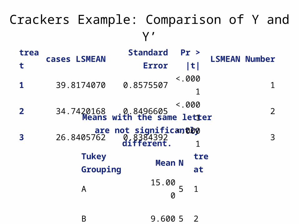
Crackers Example: Comparison of Y and Y’
Means with the same letterare not significantly different.
Tukey Grouping Mean N treatA 15.000 5 1
B 9.600 5 2
C 1.800 5 3
treat cases LSMEAN Standard Error Pr > |t| LSMEAN Number1 39.8174070 0.8575507 <.0001 12 34.7420168 0.8496605 <.0001 23 26.8405762 0.8384392 <.0001 3
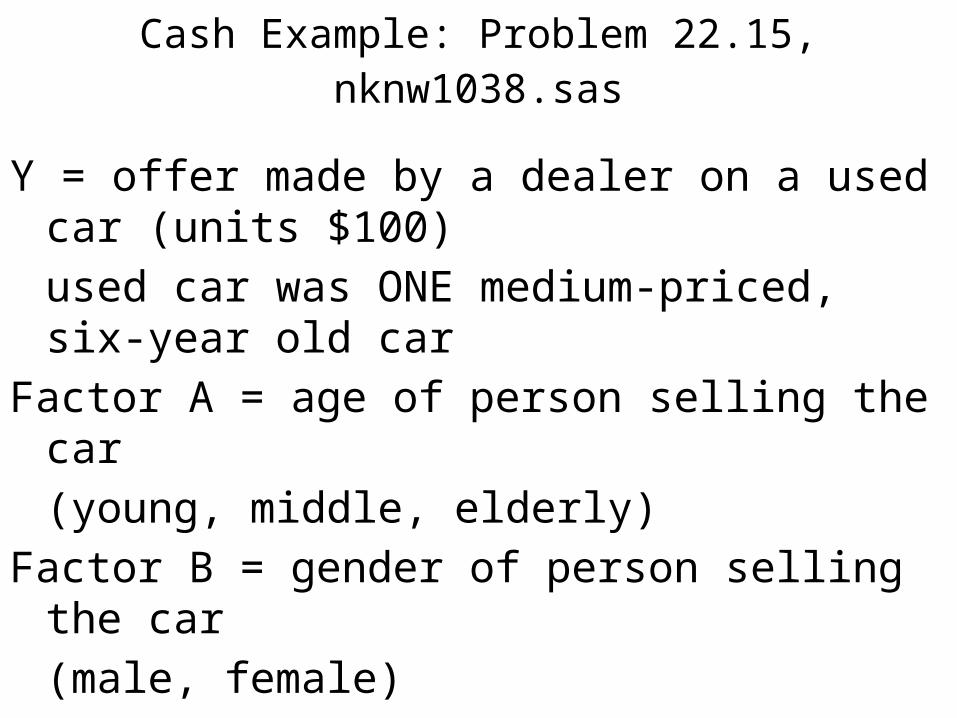
Cash Example: Problem 22.15, nknw1038.sas
Y = offer made by a dealer on a used car (units $100)used car was ONE medium-priced, six-year old car
Factor A = age of person selling the car(young, middle, elderly)
Factor B = gender of person selling the car(male, female)
n = 6X = overall sales volume for the dealer
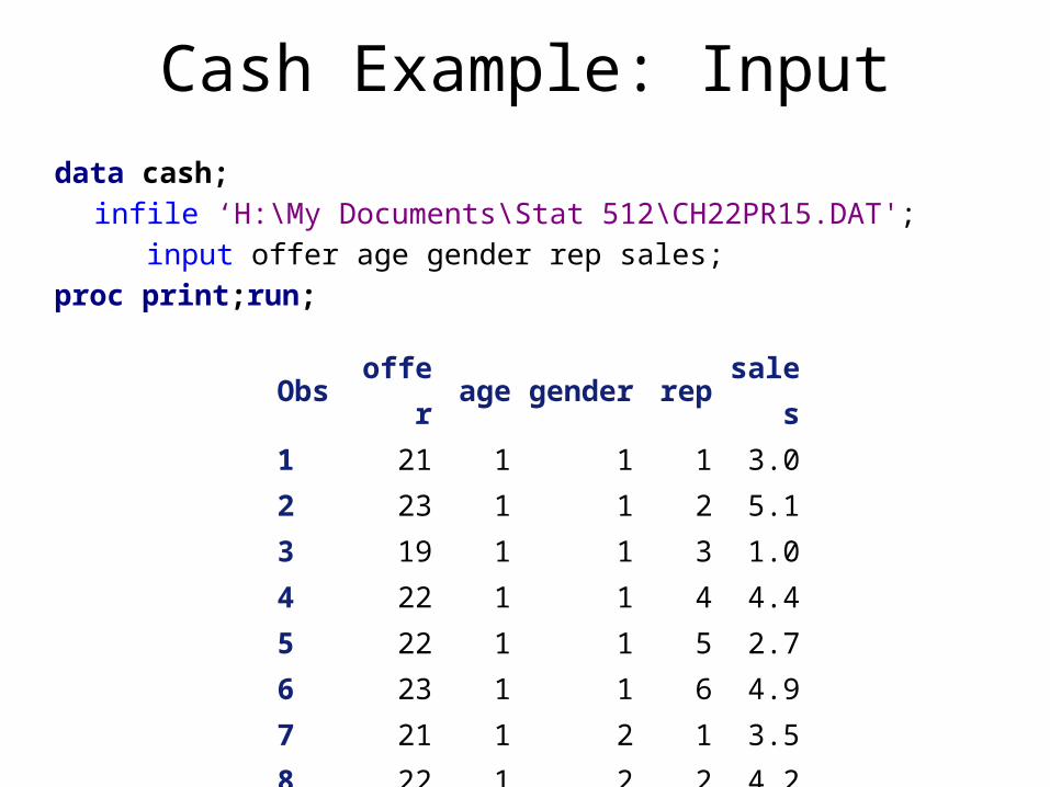
Cash Example: Inputdata cash;
infile ‘H:\My Documents\Stat 512\CH22PR15.DAT'; input offer age gender rep sales;proc print;run;
Obs offer age gender rep sales1 21 1 1 1 3.02 23 1 1 2 5.13 19 1 1 3 1.04 22 1 1 4 4.45 22 1 1 5 2.76 23 1 1 6 4.97 21 1 2 1 3.58 22 1 2 2 4.29 20 1 2 3 2.2⁞ ⁞ ⁞ ⁞ ⁞ ⁞
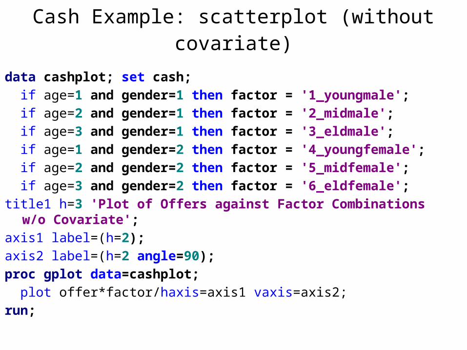
Cash Example: scatterplot (without covariate)
data cashplot; set cash; if age=1 and gender=1 then factor = '1_youngmale'; if age=2 and gender=1 then factor = '2_midmale'; if age=3 and gender=1 then factor = '3_eldmale'; if age=1 and gender=2 then factor = '4_youngfemale'; if age=2 and gender=2 then factor = '5_midfemale'; if age=3 and gender=2 then factor = '6_eldfemale';title1 h=3 'Plot of Offers against Factor Combinations
w/o Covariate'; axis1 label=(h=2);axis2 label=(h=2 angle=90);proc gplot data=cashplot; plot offer*factor/haxis=axis1 vaxis=axis2;run;
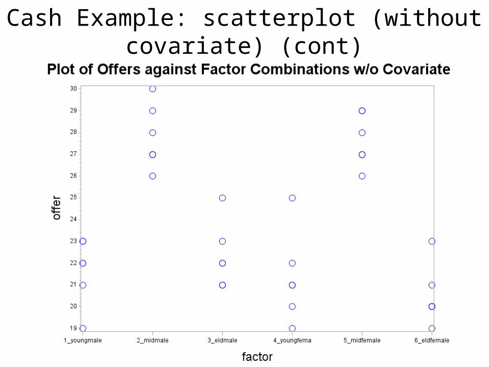
Cash Example: scatterplot (without covariate) (cont)
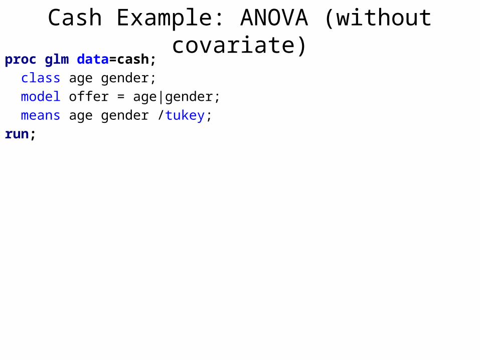
Cash Example: ANOVA (without covariate)proc glm data=cash; class age gender; model offer = age|gender; means age gender /tukey;run;
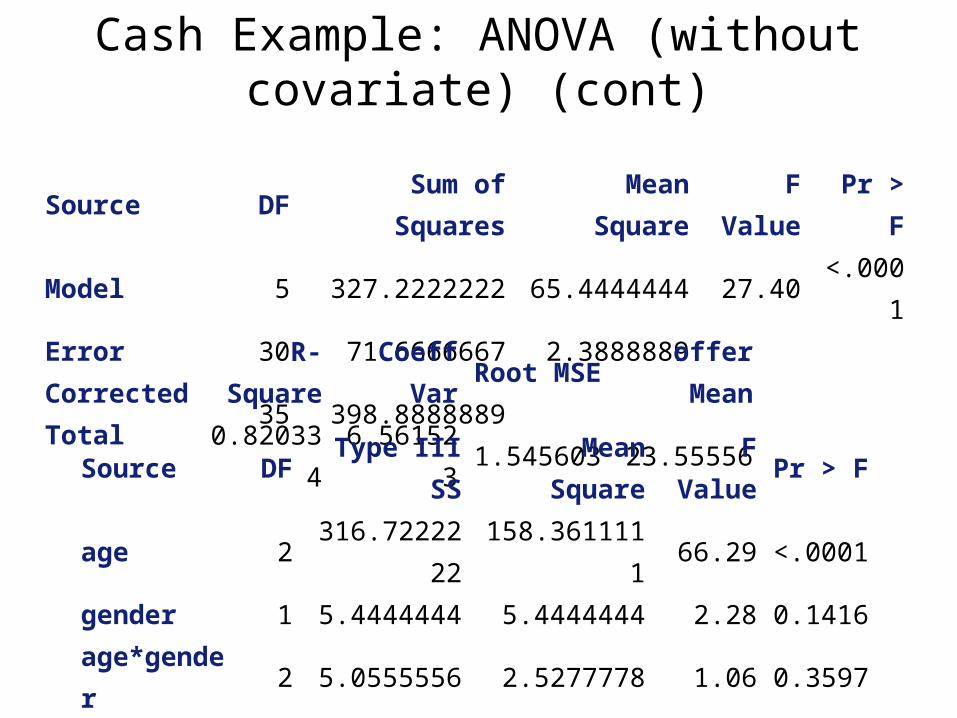
Cash Example: ANOVA (without covariate) (cont)
Source DF Sum of Squares Mean Square F Value Pr > FModel 5 327.2222222 65.4444444 27.40 <.0001Error 30 71.6666667 2.3888889Corrected Total 35 398.8888889
R-Square Coeff Var Root MSE offer Mean0.820334 6.561523 1.545603 23.55556
Source DF Type III SS Mean Square F Value Pr > Fage 2 316.7222222 158.3611111 66.29 <.0001gender 1 5.4444444 5.4444444 2.28 0.1416age*gender 2 5.0555556 2.5277778 1.06 0.3597
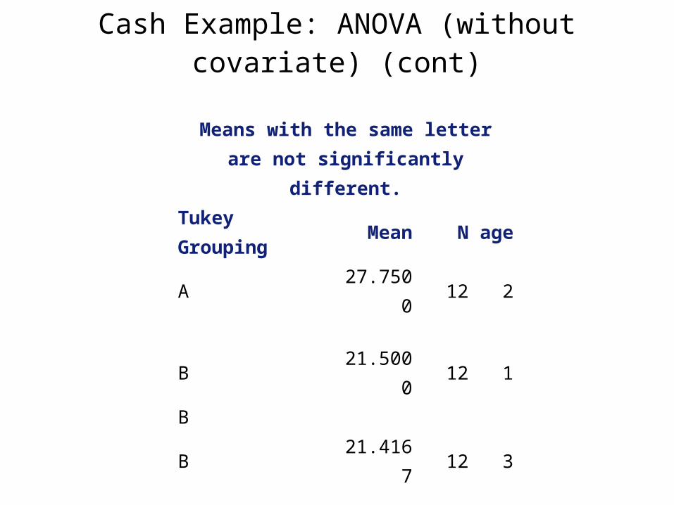
Cash Example: ANOVA (without covariate) (cont)
Means with the same letterare not significantly different.
Tukey Grouping Mean N ageA 27.7500 12 2
B 21.5000 12 1BB 21.4167 12 3
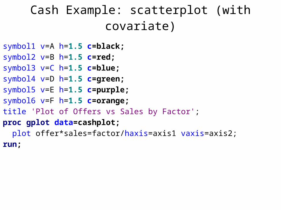
Cash Example: scatterplot (with covariate)
symbol1 v=A h=1.5 c=black;symbol2 v=B h=1.5 c=red;symbol3 v=C h=1.5 c=blue;symbol4 v=D h=1.5 c=green;symbol5 v=E h=1.5 c=purple;symbol6 v=F h=1.5 c=orange;title 'Plot of Offers vs Sales by Factor';proc gplot data=cashplot; plot offer*sales=factor/haxis=axis1 vaxis=axis2;run;
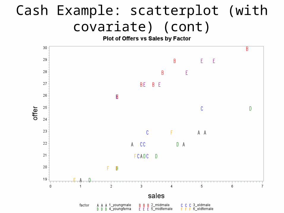
Cash Example: scatterplot (with covariate) (cont)
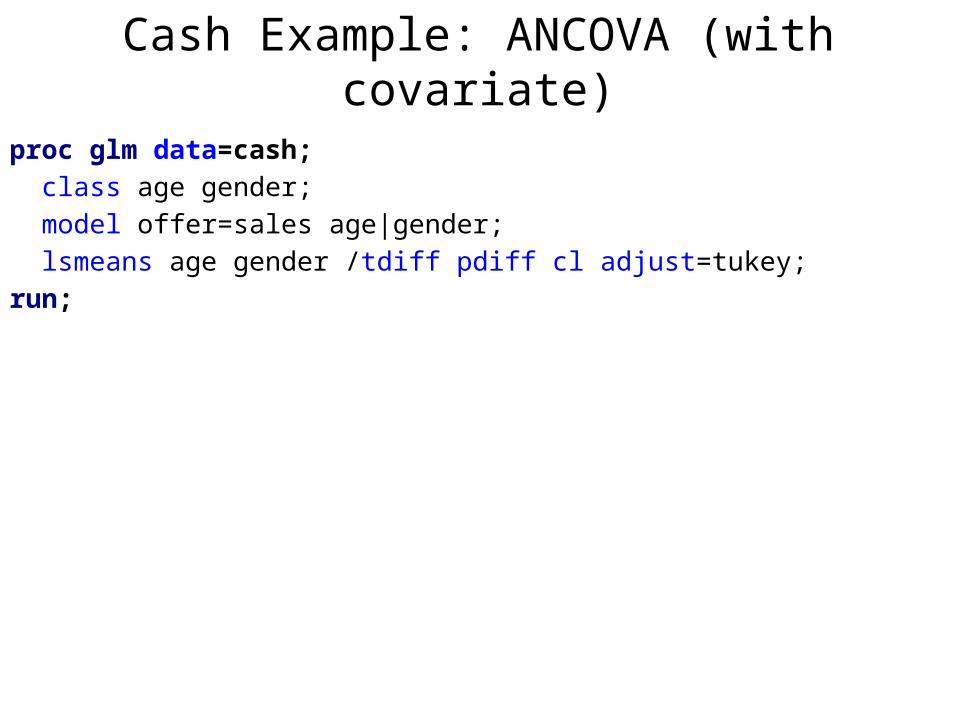
Cash Example: ANCOVA (with covariate)proc glm data=cash; class age gender; model offer=sales age|gender; lsmeans age gender /tdiff pdiff cl adjust=tukey;run;
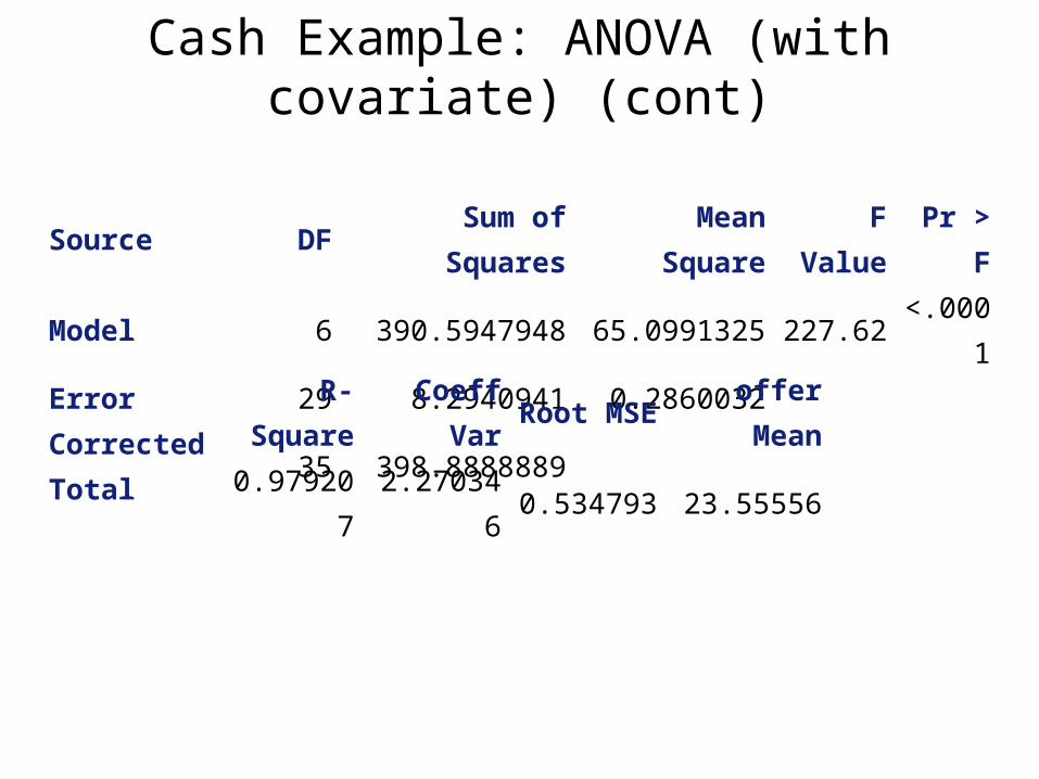
Cash Example: ANOVA (with covariate) (cont)
Source DF Sum of Squares Mean Square F Value Pr > FModel 6 390.5947948 65.0991325 227.62 <.0001Error 29 8.2940941 0.2860032Corrected Total 35 398.8888889
R-Square Coeff Var Root MSE offer Mean0.979207 2.270346 0.534793 23.55556

Cash Example: ANOVA (with covariate) (cont)
DF Type I SS Mean Square F Value Pr > Fsales 1 157.3659042 157.3659042 550.22 <.0001age 2 231.5192596 115.7596298 404.75 <.0001gender 1 1.5148664 1.5148664 5.30 0.0287age*gender 2 0.1947646 0.0973823 0.34 0.7142
Source DF Type III SS Mean Square F Value Pr > Fsales 1 63.3725725 63.3725725 221.58 <.0001age 2 232.4894513 116.2447257 406.45 <.0001gender 1 1.5452006 1.5452006 5.40 0.0273age*gender 2 0.1947646 0.0973823 0.34 0.7142
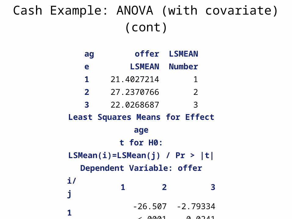
Cash Example: ANOVA (with covariate) (cont)
age
offer LSMEANLSMEAN Number
1 21.4027214 12 27.2370766 23 22.0268687 3
Least Squares Means for Effect aget for H0: LSMean(i)=LSMean(j) / Pr > |t|
Dependent Variable: offeri/j 1 2 3
1-26.507 -2.79334<.0001 0.0241
226.50696 22.55522
<.0001 <.0001
32.793336 -22.5552
0.0241 <.0001
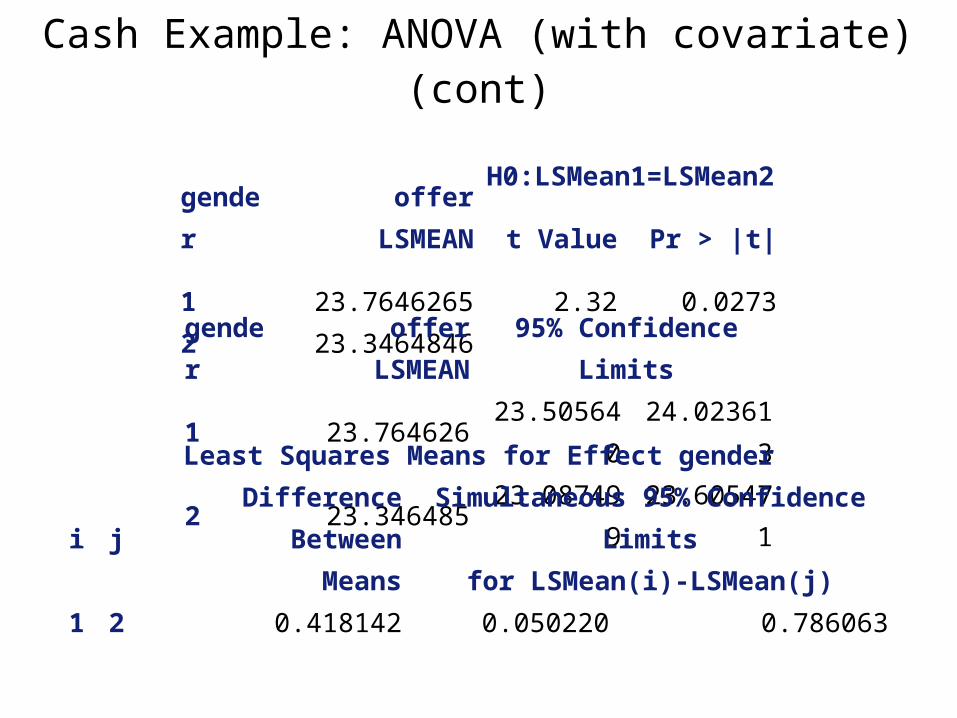
Cash Example: ANOVA (with covariate) (cont)
gender offer LSMEANH0:LSMean1=LSMean2
t Value Pr > |t|1 23.7646265 2.32 0.02732 23.3464846
gender offer LSMEAN 95% Confidence Limits1 23.764626 23.505640 24.0236132 23.346485 23.087499 23.605471
Least Squares Means for Effect gender
i jDifference Between
MeansSimultaneous 95% Confidence Limits
for LSMean(i)-LSMean(j)1 2 0.418142 0.050220 0.786063