Use of multispectral remote sensing data to map magnetite ...

Use of multispectral remote sensing data to map

magnetite bodies in the Bushveld Complex, South

Africa: a case study of Roossenekal, Limpopo.

Mthokozisi Nkosingiphile Twala

Submitted in partial fulfilment of the requirements for the degree of Master of

Science (Geology) in the faculty of Natural & Agricultural Sciences

University of Pretoria

Supervisor: Dr. James Roberts

Co-supervisors: Dr. Cilence Munghemezulu

November 2019

©© UUnniivveerrssiittyy ooff PPrreettoorriiaa

II

I went into geology because I like being outdoors and because everybody in geology seemed,

well, they all seemed like free spirits or renegades or something. You know, climbing

mountains and hiking deserts and stuff.

Kathy B. Steele


III

Declaration

I, ……………………………… declare that the thesis/dissertation, which I hereby submit for

the degree………………………at the University of Pretoria, is my own original work and has

not previously been submitted by me for a degree at this or any other tertiary institution.

Signature: _________________

Date: ______________________


IV

Acknowledgments

I wish to here record my sincere thanks to the many individuals without whom this undertaking

would have not been possible. When on numerous occasions it seemed like there was no light

at the end of the tunnel, it was the encouragement and subtle input of these individuals that led

to the eventual completion of this project. A special thanks and acknowledgment of their

contribution goes to these individuals.

First and foremost, I would like to express my deepest gratitude to Dr. James Roberts (for being

my Yoda), for believing in me and giving me the opportunity to carry-out this exciting

undertaking and for his invaluable wisdom, knowledge, and guidance every step of the way.

Secondly, I would like to sincerely thank Dr. Cilence Munghemezulu for sharing his extensive

knowledge, for his keen interest in my project, and for providing an excellent atmosphere

which to conduct research, for his Mr Miyagi-like teaching style, and for his patience and

guidance.

Thirdly, I would like to thank anyone that has taught and put up with me in the past couple of

months - my friends and family, whose encouragement and belief in me throughout has not

gone unnoticed and has subsequently brought me to this point. A special thanks to my friend

and compadre Edrich du Toit, whose value to me grows with age, and for the numerous hours

that we spent discussing our research ideas over coffee and how one day we would change the

world.


V

List of abbreviations

LANDSAT- Land Remote-Sensing Satellite (System)

TM- Thematic Mapper

MSS-Multispectral Scanner

SPOT- Satellite Pour l’Observation de la Terre

HRV- High-Resolution Visible instrument

ETM- Enhanced Thematic Mapper

ETM+- Enhanced Thematic Mapper plus

OLI- Operational Land Imager

TIRS- Thermal Infrared Sensors

NIR- Near Infrared

SWIR- Shortwave Infrared

VNIR- Visible and Near Infrared

HRS- High-Resolution Stereoscope

HRG-High Resolution Geometrical instrument

EOS- Earth Observing System

ASTER- Advanced Spaceborne Thermal Emission and Reflection Radiometer

ISODAT- Iterative Self-Organizing Data Analysis

AOI- Areas of Interest

ROI- Regions of Interest

RSE- Residual Standard Error

PCA- Principal Component Analysis

RLS- Rustenburg Layered Suite

SACS- South African Committee for Stratigraphy


VI

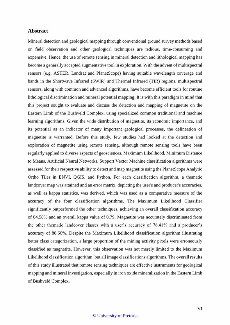
Abstract

Mineral detection and geological mapping through conventional ground survey methods based

on field observation and other geological techniques are tedious, time-consuming and

expensive. Hence, the use of remote sensing in mineral detection and lithological mapping has

become a generally accepted augmentative tool in exploration. With the advent of multispectral

sensors (e.g. ASTER, Landsat and PlanetScope) having suitable wavelength coverage and

bands in the Shortwave Infrared (SWIR) and Thermal Infrared (TIR) regions, multispectral

sensors, along with common and advanced algorithms, have become efficient tools for routine

lithological discrimination and mineral potential mapping. It is with this paradigm in mind that

this project sought to evaluate and discuss the detection and mapping of magnetite on the

Eastern Limb of the Bushveld Complex, using specialized common traditional and machine

learning algorithms. Given the wide distribution of magnetite, its economic importance, and

its potential as an indicator of many important geological processes, the delineation of

magnetite is warranted. Before this study, few studies had looked at the detection and

exploration of magnetite using remote sensing, although remote sensing tools have been

regularly applied to diverse aspects of geosciences. Maximum Likelihood, Minimum Distance

to Means, Artificial Neural Networks, Support Vector Machine classification algorithms were

assessed for their respective ability to detect and map magnetite using the PlanetScope Analytic

Ortho Tiles in ENVI, QGIS, and Python. For each classification algorithm, a thematic

landcover map was attained and an error matrix, depicting the user's and producer's accuracies,

as well as kappa statistics, was derived, which was used as a comparative measure of the

accuracy of the four classification algorithms. The Maximum Likelihood Classifier

significantly outperformed the other techniques, achieving an overall classification accuracy

of 84.58% and an overall kappa value of 0.79. Magnetite was accurately discriminated from

the other thematic landcover classes with a user’s accuracy of 76.41% and a producer’s

accuracy of 88.66%. Despite the Maximum Likelihood classification algorithm illustrating

better class categorization, a large proportion of the mining activity pixels were erroneously

classified as magnetite. However, this observation was not merely limited to the Maximum

Likelihood classification algorithm, but all image classifications algorithms. The overall results

of this study illustrated that remote sensing techniques are effective instruments for geological

mapping and mineral investigation, especially in iron oxide mineralization in the Eastern Limb

of Bushveld Complex.


VII

Publications and Proceedings

Peer-reviewed:

Forthcoming: Twala, MN., Roberts, RJ., Munghemezulu, C. Detection of magnetite in the

Rossenekal area of the Eastern Bushveld Complex, South Africa, using multispectral remote

sensing data. Submitted to South African Journal of Geology in April 2020


VIII

Table of Contents

Declaration............................................................................................................................. III

Acknowledgments ................................................................................................................. IV

List of abbreviations ............................................................................................................... V

Abstract .................................................................................................................................. VI

Publications and Proceedings ............................................................................................. VII

Table of Contents ............................................................................................................... VIII

List of Figures ........................................................................................................................ IX

List of Tables ........................................................................................................................... X

Chapter 1: Introduction .......................................................................................................... 1

1.1. General Introduction .............................................................................................................. 1

1.2. Geological setting .................................................................................................................. 2

Chapter 2: Mapping magnetite pipes in the Eastern Limb of the Bushveld Complex

using multispectral remote sensing data. ............................................................................... 9

2.1. Satellite remote sensing as an augmentative tool .................................................................. 9

2.2. Geochemical and spectral reflectance properties of magnetite ........................................... 10

2.3. Remote sensing classification algorithms ............................................................................ 13

2.4. Remote sensing sensor properties ........................................................................................ 15

Chapter 3: Data and Methods .............................................................................................. 17

3.1. Study area ............................................................................................................................ 17

3.2. Data description and pre-processing .................................................................................... 17

3.3. Field sampling ..................................................................................................................... 18

3.4. Data analysis ........................................................................................................................ 21

3.4.1 Classifications .............................................................................................................. 212122

3.4.2 Supervised classification ..................................................................................................... 22

3.4.3 Algorithm training ............................................................................................................... 24

3.5. Algorithm evaluation ........................................................................................................... 25

Chapter 4: Results.................................................................................................................. 28

4.1 Evaluating the performance of the classification algorithms............................................... 28

Chapter 5: Discussion ............................................................................................................ 38

Chapter 6: Recommendations and conclusion .................................................................... 42

References ............................................................................................................................... 44


IX

List of Figures

Figure 1: Bushveld Complex geological map and the study area demarcated (in a black

rectangle) on the Eastern Limb, modified from Cawthorn (2010). ............................. 4 Figure 2: A simplified stratigraphic succession of the Eastern Limb of the Bushveld

Complex (Impala Platinum, 2014).................................................................................. 5 Figure 3: Detailed stratigraphic sequence of the Upper Zone in the Eastern Limb of the

Bushveld Complex (Harne & Von Gruenewaldt, 1995; Maila, 2015). ........................ 7 Figure 4: Comparison of magnetite spectral reflectance signature to other Fe-Ti oxides

(Izawa et al., 2019). ........................................................................................................ 13 Figure 5: Map of the study area (Roossenekal demarcated in a black rectangle) with the

sampled landcover types in the Eastern Limb of the Bushveld Complex, with

(Planet Team, 2018). .............................................................................................. 202021 Figure 6: Sampled magnetite sites around Roossenekal that were sampled. The red dots

indicate the magnetite sites and the white dots indicate the magnetite that was used

for the validation or testing. .................................................................................. 212122 Figure 7: Land cover classification of study area using the Maximum Likelihood

classification algorithm. Different colours indicate different land class features.

Magnetite is shown in dark shade of blue. ........................................................... 313132 Figure 8: Land cover classification of study area using the Minimum Distance to Means


Magnetite is shown in dark shade of blue. ........................................................... 333334 Figure 9: Land cover classification of study area using Artificial Neural Network


Magnetite is shown in dark shade of blue. ........................................................... 353536 Figure 10: Land cover classification of study area using Support Vector Machine

learning algorithm. Different colours indicate different land class features.

Magnetite is shown in dark shade of blue. ........................................................... 373738


X

List of Tables

Table 1: Characteristics of satellite and sensors frequently used for lithological mapping

and mineral detection. ................................................................................................... 15 Table 2: Metadata for the PlanetScope images. .......................................................... 181819 Table 3: PlanetScope sensor parameters. .................................................................... 181819 Table 4: Confusion matrix for the Maximum Likelihood classification algorithm. The

overall accuracy was 84.58%, the Kappa coefficient was 0.79 and the Z-value was

731.16....................................................................................................................... 303031 Table 5: Summary of commission and omission error and producer's and user's error

for the Maximum Likelihood classification algorithm. ...................................... 303031 Table 6: Confusion matrix for the Minimum Distance to Means classification algorithm.

The overall accuracy was 71.82%, the Kappa coefficient was 0.62 and the Z-value

was 471.40. .............................................................................................................. 323233 Table 7: Summary of commission and omission error and producer's and user's error

for Minimum Distance to Means classification algorithm. ................................ 323233 Table 8: Confusion matrix for the Artificial Neural Network classification algorithm.

The overall accuracy was 62.05%, the Kappa coefficient was 0.47 and the Z-value

was 345.90. .............................................................................................................. 343435 Table 9: Summary of commission and omission error and producer's and user's error

for the Artificial Neural Network classification algorithm. ............................... 343435 Table 10: Confusion matrix for the Support Vector Machine learning algorithm. The

overall accuracy was 80.90%, the Kappa coefficient was 0.73 and the Z-value was

606.60....................................................................................................................... 363637 Table 11: Summary of commission and omission error and producer's and user's error

for the Support Vector Machine learning algorithm.......................................... 363637


1

Chapter 1: Introduction

1.1. General Introduction

Mineral exploration and geological mapping through conventional ground survey methods based on

field observation and other geological techniques are tedious, time-consuming and expensive

(Abrams et al., 1983; Martins & Gadiga, 2015; Gurugnanam et al., 2017). The wide distribution and

occurrence of some minerals in remote areas with little or no access makes map them difficult using

conventional mapping and exploration techniques (Zhang et al., 2007). Hence, remote sensing in

mineral exploration has become a generally accepted practice (Babakan & Oskouei, 2014). With the

advent of multispectral sensors (e.g. ASTER, Landsat and RapidEye) having suitable wavelength

coverage and bands in the Shortwave Infrared (SWIR) and Thermal Infrared (TIR) regions,

multispectral sensors have been considered efficient tools for routine lithological discrimination and

mineral potential mapping (Yamaguchi & Naito, 2003).

The intended use of multispectral sensors was to explore natural resources, focusing on vegetation

cover, lithological and mineral exploration. The large synoptic coverage, which gives the spatial and

integrated outlook of diverse geographical features, make optical remote sensing advantageous in

detecting potential mineral zones during the reconnaissance stage (Clark & Roush, 1984; Sabins,

1999; Rokos et al., 2000; Combe et al., 2006; Ciampalini et al., 2013; Gupta, 2017). The high-

resolution multispectral data (spatial and spectral) and digital image processing techniques have

enhanced the potential of remote sensing in demarcating and discriminating the lithology and

geological structures with better accuracy and detail. Geologists gain a double benefit from using

multispectral images because the visible and SWIR bands are sensitive to changes in soil and rock

content, making it possible to explore and map different rock and mineral types (Gupta, 2017).

The successful application of remote sensing in the exploration and mapping of iron-containing

minerals has been carried out and reported by many researchers, e.g. Rajendran et al (2007), Raja et

al (2010), and Li et al., 2016. A case in point is the detection of the lithological occurrence of iron

ore in southwestern Algeria using Landsat Enhanced Thematic Mapper Plus (ETM+) data by

(Ciampalini et al., 2013). Furthermore, the iron ore occurrence in the western part of the Wadi Shatti

district, in Libya, was successfully discriminated and delineated in the work carried out

by Abulghasem et al (2011), who used and processed ETM images by using a Maximum Likelihood

supervised classifier and band rationing.


2

It is with this paradigm in mind that this study discusses and evaluates the detection and mapping of

magnetite on the Eastern Limb of the Bushveld Complex, using specialized traditional and machine

learning algorithms. Owing to the wide distribution of magnetite and its potential as an indicator of

several vital geological processes (Klemm et al., 1985; Rajendran et al., 2007; Izawa et al., 2019), its

high iron content and significant contribution to the production of steel, the delineation and

identification of magnetite was warranted. To this end, the aim of this study was to map the

occurrence of magnetite bodies near the Roossenekal region on the Eastern Limb of the Bushveld

Complex, based on the identification of the spectral reflectance of the features. The occurrence of

magnetite was explored using common and advanced classification algorithms on the Upper Zone of

the Eastern Limb. Thereafter, the performance of common and advanced classification algorithms

was compared and contrasted. Prior to this study, no study had looked at the detection and exploration

of magnetite using remote sensing techniques in the Bushveld Complex.

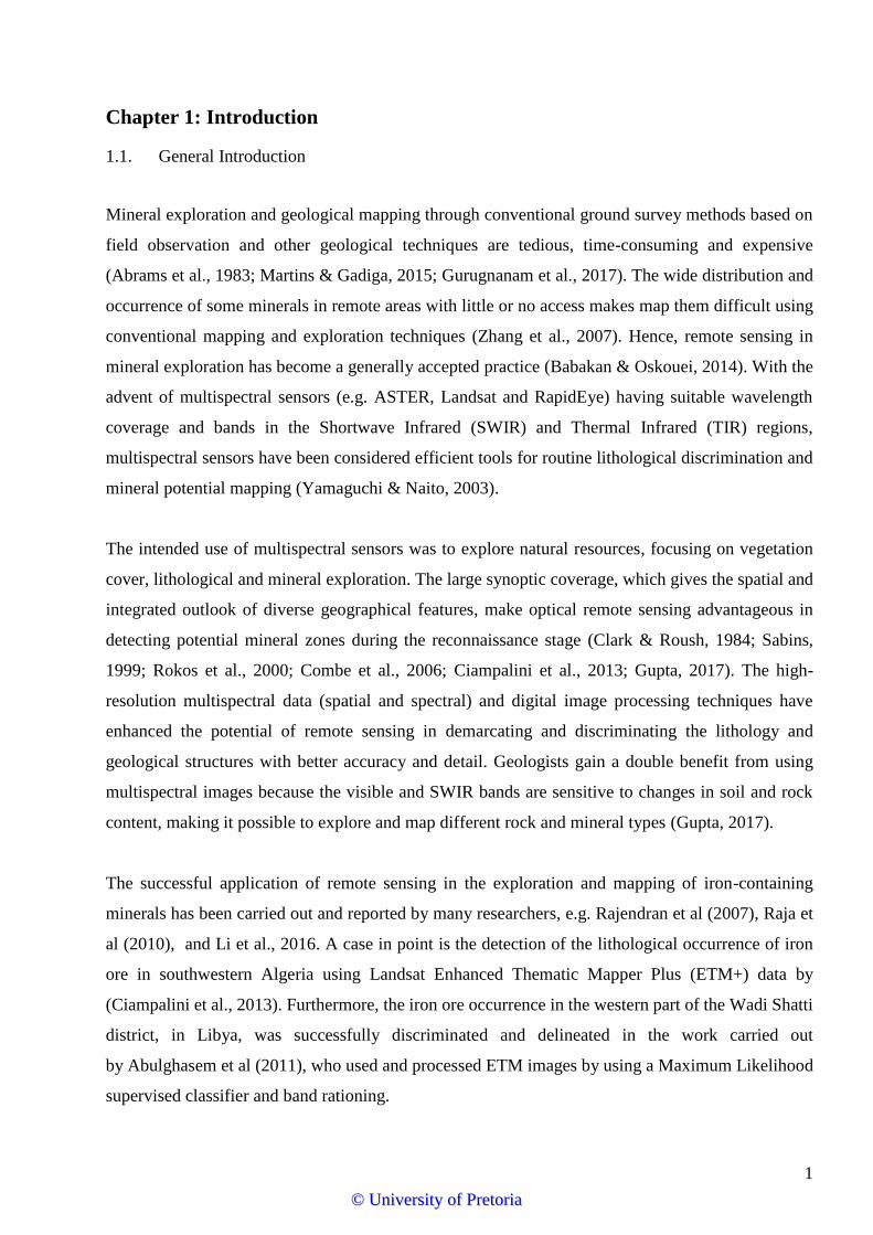
1.2. Geological setting

The Bushveld Complex is the world’s largest layered intrusion (Von Gruenewaldt, 1971; Klemm et

al., 1985; Schouwstra, Kinloch, & Lee, 2000; Fischer et al., 2016), and has been extensively studied

in the last century because of its rich platinum, palladium, rhodium, chromium, and vanadium

deposits (Willemse & Haughton, 1964; Von Gruenewaldt, 1971; Kinnaird, 2005; Tegner et al., 2006).

The Bushveld Complex spans an area of approximately 65 000 km2 (Maila, 2015). It has its

geographical centre north of Pretoria, in South Africa, at 25°S and 29°E (Maila, 2015), situated in the

northern half of the Kaapvaal craton (SACS, 1980) (as depicted in Figure 1). Harmer & Armstrong

(2000) and Schouwstra et al. (2000) postulated that approximately 0.7 to 1 million km3 of magma

was emplaced in a relatively short geological period (c. 1-3 Ma), after which the intrusion cooled to

below 650℃ in 1.02 ± 0.63 m.y. (Zeh et al., 2015). This equated to approximately 0.3-1x106 km3 of

magma per Ma, respectively. The magmatic events which induced the creation of the Bushveld

Complex (2055.91 ± 0.26 Ma) as we know it today began with the extrusion and formation of the

Rooiberg Group, which unconformably overlie the Transvaal Supergroup, from basic and acidic lavas

(Cheney & Twist, 1991). The Rashoop Suite granophyre was emplaced coeval to the Rooiberg Group.

Subsequently, the intrusion of the ultrabasic and basic lavas marked the formation of the Rustenburg

Layered Suite, which was followed by the Lebowa Granite Suite (Figure 1) (Walraven et al., 1990;

Walraven, 1993; Schweitzer et al., 1995; Kinnaird, 2005).


3

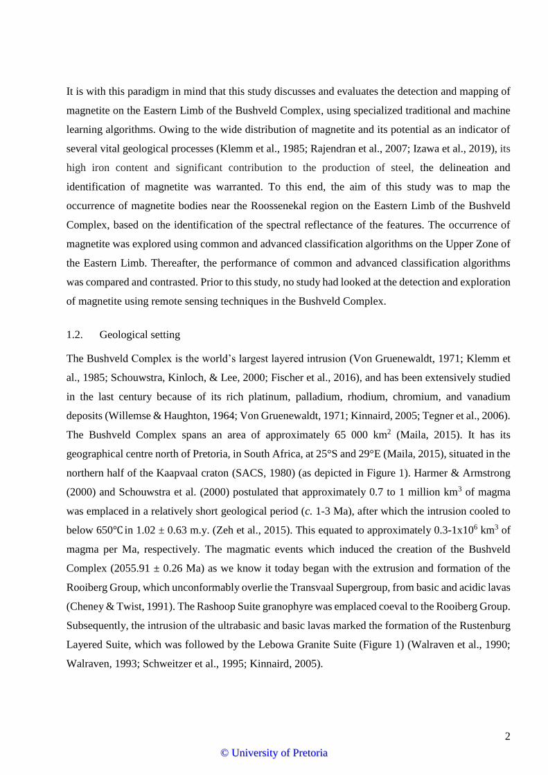
The Rustenburg Layered Suite (RLS) consists of a c. 7-9 km thick basic and ultrabasic cumulate

sequence outcropping in three limbs (the Northern, Eastern, and Western Limb) (Eales & Cawthorn,

1996; Fischer et al., 2016). This thesis focuses on the Eastern Limb. In each limb, these cumulates

are divided into their corresponding stratigraphic subdivisions, Marginal, Lower, Critical, Main, and

Upper Zones (depicted in Figure 2) (Von Gruenewaldt, 1971; SACS, 1980; Fischer et al., 2016). The

Marginal Zone consists of norites with varying proportions of clinopyroxene, quartz, biotite, and

hornblende. The Marginal Zone is often not present; however, where it does occur, its thickness

ranges from zero to hundreds of meters along the basal contact of the Eastern Limb of the Bushveld

Complex (Kinnaird, 2005).

The Lower Zone is characterized by pyroxenite, dunite, and harzburgite, with minor interstitial

plagioclase and clinopyroxene. The Lower Zone is most developed in the northern portions of the

Eastern and Western Limbs and in the southern portions of the Northern Limb, where it has the

greatest lateral extent (Schouwstra et al., 2000; Kinnaird, 2005).

The Critical Zone is approximately 1.5 km thick and hosts some of the highest concentrations of

chromitite and platinum deposits in the world in several different layers (Schulte et al., 2010). The

Critical Zone is further divided into two zones: the Lower Sub-zone and the Upper Sub-zone. The

Lower Sub-zone is a 500 m thick ultrabasic layer, comprised of a succession of orthopyroxenitic

cumulates. The 1 km thick Upper Sub-zone layer is comprised primarily of cyclic layers of chromite,

harzburgite, and norite- which has a gradational contact with anorthosite (Kinnaird, 2005; Schulte et

al., 2010). Furthermore, the Critical Zone hosts the world-renowned Platinum Group Elements (PGE)

deposits found in UG2, Merensky Reef and Platreef (Eales & Cawthorn, 1996; Grant 2015; Yuan et

al., 2017).

Measuring at approximately 3 km in thickness, the Main Zone is almost half the thickness of the RLS

(Kinnaird, 2005). It has its base on the Merensky Reef, and consists of a succession of gabbronorites

with infrequent bands of pyroxenite and anorthosite. Olivine and chromite are absent in this layer

(Chistyakova et al., 2019).

The Upper Zone is the uppermost layer in the RLS. The Upper Zone is predominately composed of

gabbros and iron-rich cumulates which host the highest concentrations of titanium-magnetite in the

world (Voordouw et al., 2009; Scoon & Mitchell, 2012; Maila, 2015). Noteworthy features in the

Upper Zone are the iron-rich cumulates which form 25 magnetitite layers in the Eastern Limb


4

(Molyneux, 1974), and a similar number in the Western and Northern Limbs. The magnetitite layers

are clustered into four groups of approximately 6 m in thickness, each consisting of seven layers, with

sharp base contacts and gradational top contacts. The Main Magnetite Layer, which is mined for

vanadium, is 2 m thick and situated near the base of the Upper Zone (Molyneux, 1974).

Figure 1: Bushveld Complex geological map and the study area demarcated (in a black rectangle) on

the Eastern Limb, modified from Cawthorn (2010).


5

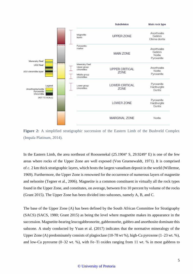
Figure 2: A simplified stratigraphic succession of the Eastern Limb of the Bushveld Complex

(Impala Platinum, 2014).

In the Eastern Limb, the area northeast of Roossenekal (25.1904° S, 29.9249° E) is one of the few

areas where rocks of the Upper Zone are well exposed (Von Gruenewaldt, 1971). It is comprised

of c. 2 km thick stratigraphic layers, which hosts the largest vanadium deposit in the world (Willemse,

1969). Furthermore, the Upper Zone is renowned for the occurrence of numerous layers of magnetite

and nelsonite (Tegner et al., 2006). Magnetite is a common constituent in virtually all the rock types

found in the Upper Zone, and constitutes, on average, between 8 to 10 percent by volume of the rocks

(Grant 2015). The Upper Zone has been divided into subzones, namely A, B, and C.

The base of the Upper Zone (A) has been defined by the South African Committee for Stratigraphy

(SACS) (SACS, 1980; Grant 2015) as being the level where magnetite makes its appearance in the

succession. Magnetite-bearing leucogabbronorite, gabbronorite, gabbro and anorthosite dominate this

subzone. A study conducted by Yuan et al. (2017) indicates that the normative mineralogy of the

Upper Zone (A) predominately consists of plagioclase (10-78 wt %), high-Ca pyroxene (1–23 wt. %),

and low-Ca pyroxene (0–32 wt. %), with Fe–Ti oxides ranging from 11 wt. % in most gabbros to


6

approximately 80 wt. % in the Main Magnetitite Layer. Hints of the recrystallized plagioclase laden

magma are given by the magmatic laminations of the large grains and the small randomly strewn

plagioclase grains around the cumulus phases or within the Fe-Ti oxide patches (Yuan et al., 2017).

The base of Upper Zone (B) is marked by the appearance of iron-rich olivine (Harne & Von

Gruenewaldt, 1995). The normative mineralogy in the Upper Zone (B) consists of plagioclase (46–

52 wt .%), high-Ca pyroxene (7–19 wt. %) and low-Ca pyroxene (8–20 wt. %), with some olivine

(1–2 wt % ) and Fe–Ti oxides (7 wt. %). The plagioclase found in the Upper Zone (B) is akin to that

found in Upper Zone (A) and has grain sizes ranging from 0.1 to 4 mm. High-Ca pyroxene which

crystallized as equant to prismatic euhedral grains, which range from 0.2 to 2 mm. In Upper Zone

(B), olivine has a prismatic shape with large sub-equant large grains (Yuan et al., 2017).

The appearance of cumulus apatite, at a depth of approximately 1000 m, marks the base of subzone

C, which is dominated by magnetite-bearing gabbro and magnetite-bearing olivine and diorite;

however, olivine-free rocks are present in the vicinity of magnetitite layers (Gruenewaldt, 1976), as

conveyed in Figures 2 and 3. Apatite appears cyclically in Upper Zone (C) and has a sub-rounded

texture, with grain sizes varying from c. 0-2 mm embedded in Fe–Ti oxides. The plagioclase, which

crystallized as tabular to euhedral grains, has a grain size range of 0.2 to 2 mm, with some planar

orientation. Unlike in Upper Zone (B), high-Ca pyroxene in Upper Zone (C) has smaller sub-equant

to subhedral grains orientated along the magma lamination, which is laden with Fe–Ti oxide

exsolutions. In Upper Zone (C), olivine crystallized as equant to irregular tabular grains with a grain

size range of 0.3–2 mm. Throughout the Upper Zone, sulphides are sparse but a majority of those

sulphides occur with magnetitite layers (Von Gruenewaldt, 1976).


7

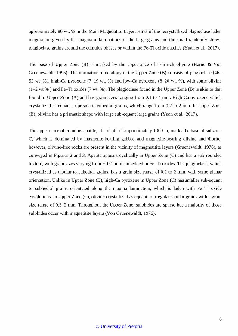
Figure 3: Detailed stratigraphic sequence of the Upper Zone in the Eastern Limb of the Bushveld

Complex (Harne & Von Gruenewaldt, 1995; Maila, 2015).

The presence of magnetitite layers throughout the entire sequence is a striking feature of the Upper

Zone. Twenty-five magnetitite layers have been identified in the Eastern Limb, with a combined

thickness of approximately 20.4 m (Tegner et al., 2006). The individual magnetitite layers range from

0.1 m to 10 m in thickness (Harne & Von Gruenewaldt, 1995). The lower three magnetitite layers


8

(layers 1-3) are located below the Main Magnetitite Layer, and Magnetite Layers 4-21 are located

above the Main Magnetitite Layer (Figure 3) (Maila, 2015). The magnetitite layers extend laterally

approximately 100 km in the Eastern Limb of the Bushveld Complex, illustrating remarkable

continuity (Cawthorn, 1994). In comparison to the upper contacts of the magnetitite layers, which

undergo a gradational change to anorthosite, the lower contacts between the magnetitite layers and

the host rocks and the underlying anorthosite are typically sharp (McCarthy et al., 1985; Reynolds,

1985). The concentration of chromitite in the Main Magnetitite Layer is indicative of diffusion-

controlled bottom crystallization, due to an upward decrease in concentration. The sharp lower

contacts of the magnetitite layers could be indicative of the abrupt onset of crystallization of

magnetite.


9

Chapter 2: Mapping magnetite pipes in the Eastern Limb of the Bushveld

Complex using multispectral remote sensing data.

2.1. Satellite remote sensing as an augmentative tool

Remote sensing is the acquisition of information and the identification of Earth-surface features or

phenomenon using reflected and emitted electromagnetic radiation (from the surface features),

assessed and measured by sensors on airborne or spaceborne platforms (Drury, 2001; Agar & Coulter,

2007; Ngcofe & Van Niekerk, 2016; Joseph & Bamidele, 2018). Optical remote sensing provides

quantitative observational parameters for large areas and hence, is an essential source of information

for many geological investigations (Rajendran et al., 2007). In the last century, remote sensing has

been extensively used in many geological applications (Abrams et al., 1983; Clark & Roush, 1984;

Chung, & Rencz, 1994; Agar & Coulter, 2007; Rajendran et al., 2007; Li et al., 2016; Manuel et al.,

2017; Joseph & Bamidele, 2018; Izawa et al., 2019). Most notably, it has been extensively applied in

geological mapping, mineral exploration, and geotechnical investigations, where it saves both time

and initial investments. In the aforementioned fields, remote sensing gives a synoptic view of the

sites of interest, which are challenging to obtain from merely field-based observations (Ngcofe &

Van Niekerk, 2016; Manuel et al., 2017).

Remote sensing employs spectral reflectivity (the measure of light that is reflected from objects on

the ground) or the spectral signature of a mineral, which is often the most useful and distinguishing

diagnostic criterion for lithological delineation (Raja et al., 2010). The spectral reflectance of objects

is depicted in images by photographic tonality and colour. The photographic tonality and colour is

influenced by the chemistry, structure, the physical conditions, and the modification of the object by

the environmental. The spectral reflectance of an object is controlled by the absorption lines, which

in turn are governed by electronic and or vibrational processes in specific minerals (Richards, 1999;

Sabins, 1999). Electronic processes involves an electron transitioning from one energy level to

another in a metal ion, whereas vibrational processes correspond to the stretching and bending of

bands due to the molecules found within the object. Therefore the lattice environment of the atoms

concerned modifies the wavelength of these absorption lines (Gupta, 2017).

Optical remote sensing makes use of the visible and near infrared (VNIR) portions of the

spectrum, which have wavelengths that range from ca 0.4 and 1 μm, to the shortwave


10

infrared (SWIR) and thermal infrared (TIR), with wavelengths of 10 μm (Gupta, 2017). Generally,

the VNIR portion of the electromagnetic spectrum is particularly useful for imaging green

vegetation, owing to the strongly absorption of the red and blue wavelengths by chlorophyll.

Minerals, on the other hand, show various absorption features in the VNIR, SWIR and TIR portion

of the electromagnetic spectrum, that relate to certain chemical components such as iron oxides

(Gupta, 2017; Shirazi et al., 2018).

The advantages and disadvantages of optical remote sensing in mineral exploration have been

extensively studied (Cloutis, 1996; Metternicht & Zinck, 2003; Agar & Coulter, 2007; Wang & Qu,

2009; Gupta, 2017). However, for similar reasons to those which encumber field geology, the

application of remote sensing for mapping geological features is fraught with both practical as well

as conceptual difficulties such as inadequate sensor spatial resolution, the reliance on exposed

lithologies for direct sensing or outcrops, and the erroneous detection of spectrally composite spectral

signatures, normally as a result of the mixing of pure end-member signatures of vegetation, soil, and

regolith (Kemp et al., 2005; Campbell & Wynne, 2011). Indeed, it is worth noting that satellite remote

sensing is not a replacement for direct fieldwork and laboratory studies. On the contrary, the best

analysis of the results is reliably acquired from the amalgamation of diverse data and from analyses

performed at different scales and perspectives. Hence, although satellite remote sensing is not a

substitute for direct fieldwork and more traditional methods, it can provide additional and crucial

information from new perspectives for preliminary geological investigations (Kemp et al., 2005).

Albeit that remote sensing tools have been to a certain extent frequently utilized in various facets of

geosciences in South Africa, with the notable exclusion of a handful of publications, there is an

absence of research regarding its specific use in opaque iron oxide mineral exploration, especially in

the Bushveld Complex.

2.2. Geochemical and spectral reflectance properties of magnetite

Magnetite is a crucial tool for paleomagnetism studies, as it carries the dominant magnetic signature

in most igneous, metamorphic and sedimentary rocks (Wingate, 1998). Additionally, magnetite is

also mined for its economic importance in the iron and steel industry (Legodi & de Waal, 2007).

Minerals that do not transmit plane polarised light due to either absorption and or dispersion of light

are classified as opaque minerals (Gurov et al., 2015; Putra et al., 2018). Sulphides and iron oxides

(i.e. minerals with a metallic luster) often have an opaque diaphaneity (Putra et al., 2018). Unlike the

exploration and detection of other iron oxides (Soe et al., 2005; Ciampalini et al., 2013; Li et al.,


11

2016; Putra et al., 2018; Shirazi et al., 2018), less than a handful of studies have had some degree of

success at mapping the lithological occurrence of the opaque mineral magnetite (Rajendran et al.,

2007; Raja et al., 2010; Izawa et al., 2019). These studies predominately made use of various

computer image enhancement techniques such as colour compositing stretched ratio, thresholding

statistical approaches, and principal component analysis (PCA).

Magnetite (Fe3O4), is a ubiquitous, opaque, spinel group mineral. Magnetite forms in igneous,

metamorphic, and sedimentary settings (Rajendran et al., 2007; Raja et al., 2010; Izawa et al., 2019).

In magmatic deposits, magnetite is generally titaniferous, occurring in close association with

pyroxene, olivine, and apatite, whereas in contact metamorphism, from rocks derived from

ferruginous sediments, it occurs with garnet and metallic sulphides such as pyrite and chalcopyrite

(Wechsler et al., 1984; Waychunas, 1991). Magnetite has the general formula of X2+Y23+O4, where

the X and Y-sites denote divalent and trivalent cations, respectively (Dare et al., 2014). The X-sites

predominately host Fe2+, Mg2+, Ca2+ and Mn2+, whilst the Y-sites predominately host Si4+, Al3+, Ti4+,

Cr3+, V5+, and Fe3+ elements (Dare et al., 2014). Trace elements found in the different sites indicate

the provenance and conditions in which magnetite was formed (Dare et al., 2014). However, the

regeneration of minerals during hydrothermal processes may modify magnetite, and hence

consideration needs to be taken when using magnetite as a proxy for the genesis and formation of

related deposits.

The spectral reflectance of a rock unit at the visible and near visible wavelength depends on the

composition of the outermost 100 μm material (Gupta, 2017), and is controlled to a large extent by

the presence of weathering products which are ubiquitous to the magnetite bodies (which outcrop as

very hard, generally dark, medium to coarse grains with euhedral to subhedral shapes) of the

Roossenekaal area. Under reflected light, magnetite is isotropic (Legodi & de Waal, 2007; Rajendran

et al., 2007). In the presence of water, magnetite weathers along its margins, altering to hematite and

limonite, which have a low to high order birefringence. Because of the contamination with these

minerals, the absolute spectral response may be correlated with the absorption bands of hematite and

limonite. Typically, in weathered iron oxide products the Fe3+ charge transfer in the bond is

responsible for the absorption at wavelengths shorter than about 0.55 μm. This charge transfer is

responsible for the visible red colour which is characteristic of ‘iron staining’ (Rajendran et al., 2007;

Gupta, 2017). Furthermore, ferric irons produce diagnostic spectral absorption near 0.7 μm and 1.0

μm region of the electromagnetic spectrum due to electronic transitions, which may be of significance

feature in remote sensing.


12

The spectral reflectance of magnetite has been extensively studied in the visible and near-infrared

spectral range (Morris et al., 1985; Wagner et al., 1987; Cloutis et al., 2008; Izawa et al., 2019), but

most studies used too few samples of magnetite to acquire a reliable spectral reflectance of magnetite

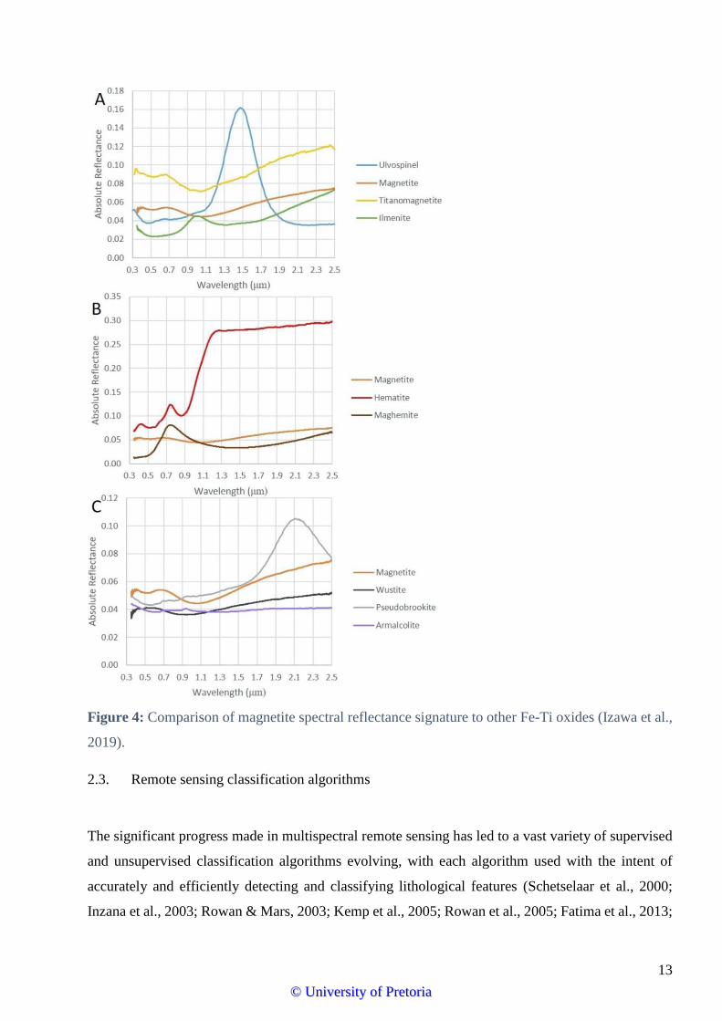
(Morris et al., 1985; Wagner et al., 1987; Cloutis et al., 2008). According to Hunt, (1971) and Izawa

et al. (2019), the spectral signature of magnetite in the ultraviolet, visible, and near-infrared is akin

to that of titanomagnetite and wüstite but distinct from other Fe-Ti oxides such as ilmenite, haematite,

ulvospinel, maghemite, pseudobrookie, and armalcolite (indicated in Figure 4), suggesting the

plausibility of the detection and mapping of magnetite using remote sensing techniques. Previous

work by Hunt, (1971) focusing on the influence of grain size on the spectral signature of two

magnetite, one titaniferous, and four grain size samples, yielded low spectral reflectances. This was

an expected result of analysing an opaque mineral. This observed phenomenon was caused by the

structural absorption of the incident light projected to the sensor by the fine magnetite grains.

However, an increase in spectral reflectance was directly proportional to the increase in grain size

(Hunt, 1971).


13

Figure 4: Comparison of magnetite spectral reflectance signature to other Fe-Ti oxides (Izawa et al.,

2019).

2.3. Remote sensing classification algorithms

The significant progress made in multispectral remote sensing has led to a vast variety of supervised

and unsupervised classification algorithms evolving, with each algorithm used with the intent of

accurately and efficiently detecting and classifying lithological features (Schetselaar et al., 2000;

Inzana et al., 2003; Rowan & Mars, 2003; Kemp et al., 2005; Rowan et al., 2005; Fatima et al., 2013;


14

Babakan & Oskouei, 2014; Shirazi et al., 2018). Supervised classification, which entails the assigning

of samples of identical pixels to classes that exhibit the same tonality, texture, and shape to each class

has been met with tremendous success in geological mapping. Traditional supervised methods of

classifying remote sensing data such as the Maximum Likelihood and Minimum Distance to Mean

classification algorithm are commonly compared in terms of their predictive accuracies to more

advanced classification algorithms such as Decision Trees, Fuzzy C-Mean, Support Vector Machines,

and Artificial Neural Networks. The image classification algorithm Maximum Likelihood has wide-

ranging popularity in its application in remote sensing image classification (Jensen, 2005). The

classification algorithm is based on a parametric approach that assumes a normal Gaussian

distribution of the selected classes (Kavzoglu & Reis, 2008; Mondal et al, 2012). The Minimum

Distance to Means classification algorithm is another common parametric classification algorithm,

which classifies unknown pixels to the class with the mean arithmetically closest to them (Wacker &

Landgrebe, 1972).

Decision Trees, Fuzzy C-Mean, Support Vector Machines, and Artificial Neural Networks are just

some of the few well-known non-parametric classification algorithms. The predominately used non-

parametric algorithms are Artificial Neural Networks and Support Vector Machines. Artificial Neural

Networks are an artificial intelligence-based classification algorithm that simulates pattern

recognition, identification, classification, and control system similar to biological neural networks

(Haykin, 1994; Bachri et al., 2019). Unlike the Maximum Likelihood classification algorithm,

Artificial Neural Networks can classify multi-modal or landcover types that do not assume a normal

Gaussian distribution in spectral space. Support Vector Machines are a group of supervised

classification algorithms that compare favourably with more established common remote sensing

algorithms. Support Vector Machines are considered to be heuristic algorithms founded on statistical

theory, used for classification and regression problems (Vapnik, 1999; Vapnik, 2013). The

classification accuracy of Support Vector Machines may vary contingent on the selected kernel

function and its parameters (Kavzoglu & Colkesen, 2009; Yu et al., 2012).


15

2.4. Remote sensing sensor properties

To further increase the landcover discrimination ability of classification algorithms, various high-

resolution satellite sensors have been launched, with some having the capability of generating

remote sensing imagery with a spatial resolution of 4 m or less in multispectral mode. Table 1

briefly lists some characteristics of known satellites and sensors predominately used for lithological

mapping and mineral detection.

Table 1: Characteristics of satellite and sensors frequently used for lithological mapping and

mineral detection.

Spatial resolution specifies the dimensions of the satellite image pixels, i.e. the higher or finer the

spatial resolution, the more detail the sensor is able to provide of the ground cover. The spatial

resolution is contingent on the desired object of observation. The spectral resolution determines the

number of spectral bands reflected radiance that can be collected by the sensor or the range of

wavelengths a single band covers. The more bands a sensor has, the better equipped it is to identify

and characterise natural materials (Congalton, 2001; Gupta, 2017).

Radiometric resolution refers how fine a sensor divides up the radiance it receives in each band and

therefore is an indicator of the amount of information is in contained in each pixel. The finer the

radiometric resolution the greater the sensitivity of radiation the sensor is able to detect (Gupta,

2017). However, owing to the difficulty and exorbitant costs of obtaining imagery with an extremely

high resolution, it is often necessary to identify resolutions which are paramount for a project, in a

process known as “trade-offs”. Either the spatial resolution is high, but the spectral and radiometric

resolution are low or vice versa. Since the dimensions of the smallest magnetite bodies recorded for

Satellite Sensor Launch Spectral resolution Spatial

resolution (m)

Country of

ownership

LANDSAT TM,

MSS 1976

7 visible and 1 thermal IR band; 0.50-

12.5 µm spectral resolution 30 - 80 USA

SPOT HRV 1986 3 visible and 1 IR band; 0.50-0.73 µm

spectral resolution 10 - 20 France

RapidEye Jena-

Optronik 2008

4 visible and 1 IR band; with 0.44-0.88

µm spectral resolution

5 USA

LANDSAT-7 ETM 1999

8 visible and 1 thermal IR band; 0.45-

12.5 µm spectral resolution

15 - 60 USA

LANDSAT-8 OLI,

TIRS 2013

9 visible, 1 and thermal IR band; 0.433-

12.50 µm spectral resolution

15, 30, 100 USA

SPOT-5 HRS,

HRG 2002

4 visible and 1 IR band; 0.50-0.71 µm

spectral resolution 10, 20 France

TERRA

(EOS AM-1) ASTER 1999

14 visible and 5 IR bands; 0.53-11.65

µm spectral resolution 15 - 90 USA


16

this study were approximately 3 m (7.07 m2), a sensor with spatial resolution of 3 m with a fine

spectral and radiometric resolution to distinguish and detect the slightest changes in radiance from

magnetite and other geological material was required. However, as conveyed in Table 1, it is not

plausible to have a sensor with high spatial, spectral, and radiometric resolution.

However, for this study, offerings from an American based private company provided the some of

the best trade-offs for the detection of magnetite relative to the sensor in Table 1. Planet Team (2018),

offers three earth observation products: a Basic Scene product, an Ortho Scene product, and an Ortho

Tile. Planet Team (2018) has a complete constellation of over 150 satellites imaging the entire surface

of the earth every day with a spatial resolution of 3 m, a spectral resolution of 4 bands (blue, green,

red and NIR), and a radiometric resolution of 16-bits, with a position accuracy of less than 10 m

residual standard error (RSE) and a daily revisit capability.

This study has mainly employed the use of supervised classification algorithms based on awareness

of previous successes and performances. The remote sensing algorithms that were used in this study

are Maximum Likelihood, Minimum Distance to Means, Artificial Neural Networks, and Support

Vector Machines. Along with detecting the lithological occurrence of magnetite on the Eastern Limb

of the Bushveld Complex, this study has sought to determine the overall efficiency of the different

classification algorithms with the PlanetScope imagery. The accuracy of each algorithm was assessed

using the collected reference data. User’s and producer’s accuracy, along with errors of commission

and omission were used as comparative indices of measure of the efficiencies of each of the different

supervised classification algorithms.

As advanced data analysis tools, for this particular study we expect advanced classification algorithms

(Artificial Neural Networks and Support Vector Machines) to be more equipped for the detection and

mapping of magnetite, able to map the different classes more accurately than common traditional

classification algorithms (Maximum Likelihood and Minimum Distance to Means), and to depict a

more realistic representation of the different classes on the ground. Advanced classification

algorithms have been generally noted to outperform common traditional classification algorithms,

especially with projects that have a limited number of training samples for each of the input classes

(Otukei & Blaschke, 2010; Szuster et al., 2011; Mondal et al., 2012; Omeer et al., 2018). This

expectation is contingent on the high accuracy of advanced classification algorithms when the training

data is randomly dispersed across the region under investigation (An et al., 1994; Omeer et al., 2018;

Singer & Kouda, 1996, 1997b).


17

Chapter 3: Data and Methods

3.1. Study area

As noted by Molyneux (1974), Willemse & Haughton (1964), and Scoon & Mitchel (2012), the

magnetite bodies observed and reported in the Upper Zone of the Eastern Limb of the Bushveld

Complex predominately occur in the Roossenekal area. The Roossenekal area is situated at 700 to

1100 m.a.s.l and is characterised by undulating to flat plains dominated by Bushveld vegetation, an

intermediate stage vegetation between Shrubveld and Woodland (Van Rooyen & Bredenkamp, 1996;

Low & Rebelo, 1998; Rutherford et al., 2006). Roossenekal and the surrounding area host a diverse

amount of plant species over a short distance, which is a trait similar to the Cape Floristic Kingdom

(Rutherford et al., 2006). The diverse geology of the area could be the contributing factor to the floral

diversity. Although, the Roossenekal area is situated in close proximity to the north-eastern

Drakensberg Escarpment, which is cool and characterised by copious amounts of rainfall, the

Roossenekal lies in a semi-arid savanna within a warm and dry valley. Roossenekal has a mean annual

rainfall of 400 mm and temperatures ranging from -4℃ to 38℃ (Van Rooyen & Bredenkamp, 1996;

Siebert et al., 2002a, 2002b).

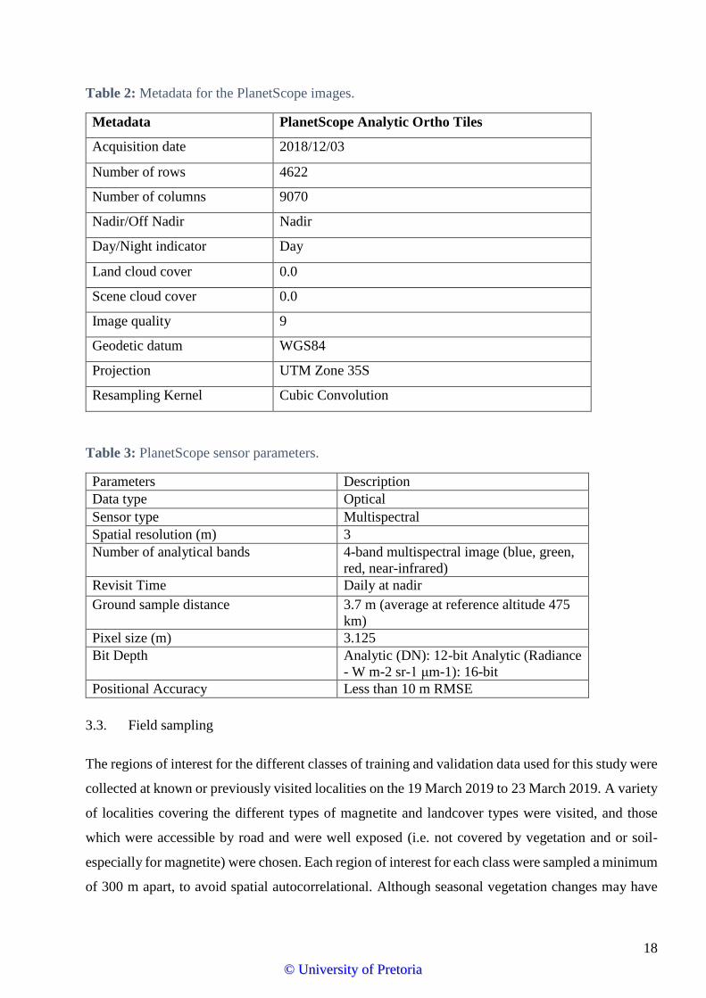
3.2. Data description and pre-processing

The PlanetScope Analytic Ortho Tiles used for the creation of the thematic map of the study site and

for the detection of magnetite were sourced from Planet Explorer (Planet Team, 2018), for the date

03 December 2018, which had the highest image quality and the lowest land and scene cloud cover

closest to the date of sampling. Furthermore, the choice of the PlanetScope Analytic Ortho Tiles was

contingent on the vegetation cover on the chosen magnetite sites (explained in the next section). The

metadata for the set of PlanetScope Analytic Ortho Tiles is selectively displayed in Table 2, and the

parameters for the PlanetScope Sensor are given in Table 3. The PlanetScope Analytic Ortho Tiles

are corrected for geometric-, sensor-, and radiometric interferences and have been aligned to a

cartographic map projection (UTM WGS 84). Image mosaicking was applied, using the pixel-based

mosaicking function, for the ortho-tiles covering the area of interest. To better extract the different

landcover types or classes, the false-colour composition of the mosaicked ortho-tile image was used

(Gupta, 2017; Omeer et al., 2018).


18

Table 2: Metadata for the PlanetScope images.

Metadata PlanetScope Analytic Ortho Tiles

Acquisition date 2018/12/03

Number of rows 4622

Number of columns 9070

Nadir/Off Nadir Nadir

Day/Night indicator Day

Land cloud cover 0.0

Scene cloud cover 0.0

Image quality 9

Geodetic datum WGS84

Projection UTM Zone 35S

Resampling Kernel Cubic Convolution

Table 3: PlanetScope sensor parameters.

Parameters Description

Data type Optical

Sensor type Multispectral

Spatial resolution (m) 3

Number of analytical bands 4-band multispectral image (blue, green,

red, near-infrared)

Revisit Time Daily at nadir

Ground sample distance 3.7 m (average at reference altitude 475

km)

Pixel size (m) 3.125

Bit Depth Analytic (DN): 12-bit Analytic (Radiance

- W m-2 sr-1 μm-1): 16-bit

Positional Accuracy Less than 10 m RMSE

3.3. Field sampling

The regions of interest for the different classes of training and validation data used for this study were

collected at known or previously visited localities on the 19 March 2019 to 23 March 2019. A variety

of localities covering the different types of magnetite and landcover types were visited, and those

which were accessible by road and were well exposed (i.e. not covered by vegetation and or soil-

especially for magnetite) were chosen. Each region of interest for each class were sampled a minimum

of 300 m apart, to avoid spatial autocorrelational. Although seasonal vegetation changes may have


19

influenced some activities such as farming in the area, fieldwork was constrained by logistical and

scheduling constraints.

Global Positioning System (GPS) coordinates covering the circumference of the area of interest were

collected together with a brief description of the setting that the land-cover type was found in, as well

as a sample number. The GPS data collected was converted to ground reference areas or polygon

delineations of the shape of each of the areas of interest, using QGIS 2.18 (QGIS Development Team,

2015). The ground reference data was used to train the algorithms used in ENVI and Python

(Continuum Analytics, 2019). Accessibility to certain areas of interest and time were the main

limitations in attaining a vast array of ground reference data. Hence, auxiliary GPS coordinate data

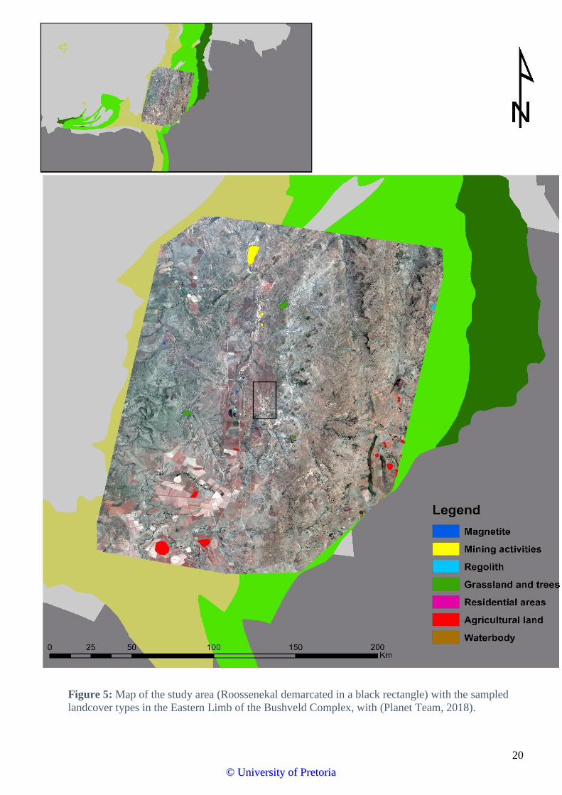
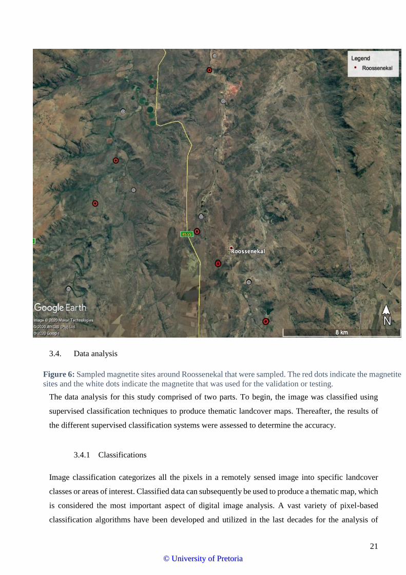
was acquired from Google Earth imageries. The 120 areas of interest were combined into seven

classes (Agricultural land, Grassland and trees, Residential areas, Waterbodies, Mining Activities,

Regolith, and Magnetite) and divided into training data and validation data (as indicated in Figure 5

and 6 (for magnetite)).


20

Figure 5: Map of the study area (Roossenekal demarcated in a black rectangle) with the sampled

landcover types in the Eastern Limb of the Bushveld Complex, with (Planet Team, 2018).


21

3.4. Data analysis

The data analysis for this study comprised of two parts. To begin, the image was classified using

supervised classification techniques to produce thematic landcover maps. Thereafter, the results of

the different supervised classification systems were assessed to determine the accuracy.

3.4.1 Classifications

Image classification categorizes all the pixels in a remotely sensed image into specific landcover

classes or areas of interest. Classified data can subsequently be used to produce a thematic map, which

is considered the most important aspect of digital image analysis. A vast variety of pixel-based

classification algorithms have been developed and utilized in the last decades for the analysis of

Figure 6: Sampled magnetite sites around Roossenekal that were sampled. The red dots indicate the magnetite

sites and the white dots indicate the magnetite that was used for the validation or testing.


22

remotely sensed data (Otukei & Blaschke, 2010). Pixel-based classification approached employ the

usage of spectral signatures of individual pixels and algorithms to classify each pixel to a thematic

class (Rawat et al., 2013).

Classification algorithms can be categorized as either common or advanced. The most notable and

most often used common classification algorithms include the K-means, Iterative Self-Organizing

Data Analysis (ISODAT), Maximum Likelihood classifier, Minimum Distance to Means (Richards,

1999; Sabins, 1999; Lillesand & Kiefer, 2000; ERDAS, 2005; Otukei & Blaschke, 2010; Mather &

Koch, 2011), while advanced algorithms include Support Vector Machines, and Artificial Neural

Networks classifier (Foody, 1996; Kim & Pang, 2003; Mitra et al., 2004; Verbeke, Vancoillie et al.,

2004). However, it is worth noting that there is no universal classification method that is efficient

with all regions, therefore choosing the correct method is essential in ensuring better accuracy (Herold

et al., 2008). Several imperative considerations govern the physiognomy of landcover information,

which include purpose, thematic content, scale, data, and processing and analysis algorithms (Cihlar,

2000).

3.4.2 Supervised classification

Not all supervised image classification algorithms could be evaluated. Some of the common

traditional and advanced algorithms were used and evaluated, namely: Maximum Likelihood

classifier, Minimum Distance to Means, and the advanced classification algorithms (Support Vector

Machines, and Artificial Neural Networks classifier). In the section that follows, a brief explanation

of the four algorithms will be explained.

The Maximum Likelihood classification algorithm has been the most frequently used data driven

parametric classifier in remote sensing for data classification (Foody et al. 1992; Kavzoglu & Reis,

2008; Otukei & Blaschke, 2010; Jia et al., 2011; Mondal et al., 2012). The Maximum Likelihood

classification algorithm assumes that a hyper-ellipsoid decision volume can be utilized in

approximating the profile of the data clusters. Additionally, for a given unidentified pixel, the

likelihood or probability of membership in each class is predetermined using the covariance matrix

and the prior probability (i.e. the mean feature vectors of the classes (Chien, 1974). For normally

distributed data, the Maximum Likelihood classification algorithm provides better predictive

accuracy than the other parametric classifiers; however, for data that is not normally distributed the

predictive accuracy may be unsatisfactory (ERDAS, 2005; Otukei & Blaschke, 2010).


23

The Minimum Distance to Means classification algorithm classifies a pixel by calculating the

arithmetic distance between itself and each of the other different landcover categories. The pixel is

subsequently allocated to the class with the shortest distance to the mean, however, when the relative

distances between the selected pixels and each of the landcover classes is higher than the average

distance determined by the analyst, the pixel is categorized as unidentified (Mather & Tso, 2016).

Notably, the Minimum Distance to Means classification algorithm does not take into account the

different degrees of variance within the spectral reflectance data, i.e. the close proximity of spectral

classes may inadvertently lead to higher variances. Consequently, the Minimum Distance to Means

classification algorithm has often been observed not to correctly classify the landcover features by

Al-Ahmadi & Hames (2009), Murtaza & Romshoo (2014), Walton (2015), and Marapareddy et al

(2017).

An artificial neural network is a biologically inspired and adaptive algorithm that is designed to

recognise patterns that are numerical, contained in vectors and real-world data (Vapnik, 1999;

Brown et al., 2000; Nagy et al., 2002; Verbeke et al., 2004; Rodriguez-Galiano et al. 2015). The

algorithm consists of neurons, the simple processing elements, reciprocally connected by links

associated with numeric coefficients which indicate the relative strength of each connection (Brown

et al., 2000). Once the training data has been assigned into the algorithm, the information is

disseminated throughout the network in the form of numeric coefficients (i.e. the weight values)

that have been altered as a result of learning. Although artificial neural networks have been used in

other facets of exploration geology, such as petroleum exploration (Osborne, 1992; Taggart &

Gedeon, 1996), few studies have described its application in mineral surveys (Gilles et al., 1992;

Singer & Kouda, 1996, 1997a, 1997b) or geological mapping (An et al., 1994). In this study the

artificial neural network classification algorithm was run with a training threshold contribution of

0.5 and 1000 training iterations (to avoid overfitting). The training threshold contribution adjusts

the weight between nodes and reduces the amount of error from the nodes. A 0.5 training threshold

contributor lead to a better image classification.

The Support Vector Machine supervised classification algorithm is a data-driven technique that is

based on statistical learning theory (Vapnik, 1999), and has been further developed in many other

classification applications in the past decade. The algorithm aims to determine the location of decision

boundaries that optimizes the greatest separation between the different landcover classes (Pal &

Mather, 2005; Vapnik, 1999; 2013). Considering the example of two classes which are linearly

separated, the Support Vector Machine selects the linear decision boundary that reduces the


24

generalization error and leaves the greatest distance from the hyperplane or margin between the two

classes (i.e. segregates and leaves the largest distance between the classes and the hyperplane)

(Vapnik, 1999; 2013). The data points contiguous to the hyperplane that are used to measure the

distance from the hyperplane or margin are termed ‘support vectors’. The Support Vector Machine

creates and uses the hyperplane that maximizes the margin, whilst minimizing the generalization error

or the number of misclassifications (Pal & Mather, 2005). The choice of kernel function of Support

Vector Machine classification algorithm (linear kernel, polynomial kernel, radial basis function

kernel, and sigmoid kernel) is integral to its accuracy training and classifying remote sensing imagery.

In this study, the radial basis function kernel was used because the remote sensing data was not

linearly distributed.

3.4.3 Algorithm training

The image processing procedure involves a series of operations to classify the selected satellite

imagery. QGIS (QGIS Development Team, 2015) was used to manually delineate the landscape into

polygons of homogenous training sites. ENVI 5.5 software (Exelis Visual Information Solutions,

2017) and Python (Continuum Analytics, 2019) were used in all the above mentioned pre-processing,

processing and post-processing steps.

The first phase of processing required the categorization of the different pixels into information

classes or training sites based on reflectance characterization. Once the statistical characterization or

signature analysis had been completed for each landcover class, the image was classified by

inspecting the spectral reflectance of each pixel and determining which of the training sites or sampled

landcover spectral signatures it resembles most. For each of the 7 different training sites (Agricultural

land, Grassland and trees, Residential areas, Waterbodies, Mining activities, Regolith, and Magnetite)

a minimum of six areas of interest (AOI) were generated. For each of the classes, a homogenous

spectral signature was acquired from different localities on the map depicting the same training site.

These parameters for training the algorithms were carefully digitized since they are very sensitive

and strongly influence the algorithms' predictive accuracy (Rodriguez-Galiano et al., 2015).

Training data, as well as validation data, was digitized in QGIS (QGIS Development Team, 2015)

using a false composite of PlanetScope Analytic Ortho Tile band 1 (red), band 2 (green), band 3

(blue), and band 4 (near-infrared) using visual inspection, field observations of each site, Google

Earth imagery from 2018 (Google Earth, 2018), and an ancillary landcover map from ArcGIS Online


25

to assign pixels to each of the six out of seven classes (magnetite not included). The shapefile

containing the spectral signatures of the training-data and validation-data for all classes was

subsequently imported to ENVI (Exelis Visual Information Solutions, 2017) to create regions of

interest (ROIs). The pixel count of each of the ROIs were log transformed (for the data to be normally

distributed and to meet algorithm assumptions) and used in the Maximum Likelihood, Minimum

Distance, and Artificial Neural Networks classification algorithms. Untransformed ROIs were used

for Support Vector Machines classification algorithms to catalogue the range of spectral data in the

entire satellite image. The classified images were further smoothed using the clump classes function

with a dilate and erode kernel value of three for both columns and rows to reduce the number of

misclassified pixels.

3.5. Algorithm evaluation

The assessment of the accuracy and fitness of image classification algorithms has become a central

component of studies that have sought to compare the abilities of the different algorithms in

discriminating different classes (Congalton et al., 1983; Congalton, 2001; Congalton & Green, 2002;

Mather & Koch, 2011; Mather & Tso, 2016).The aim of performing an accuracy assessment is to

assess the fitness for use of the classified data. The classified map is compared to reference points

where the classes of the landcover have been already been determined. The accuracy of the

classification is then calculated. Most often the error matrix technique is used as a method for

assessing the accuracy and fitness of the thematic map for a particular purpose. Accuracy assessments

determines the quality and accuracy of the information consequent from remotely sensed data. The

accuracy of the thematic map needs to be evaluated so that the ultimate user is made conscious of any

potential problems that may be associated with the use of the thematic map. The end-product of the

image classification process is a landcover or thematic map.

As previously introduced, an error matrix is a matrix that depicts the number of pixels or sample units

that were correctly classified to a particular category in comparison to pixels or sample units

belonging to another particular category being assigned to a different category or class (Congalton &

Green, 2002). The columns of the error matrix represent the reference data or validation data

(normally generated from ground observations and measurements and or ancillary remote imagery),

and the rows represent the data attained from the classification of the remotely sensed imagery. The

error matrix not only depicts the map accuracy but the error as well (Congalton, 2001; Congalton &

Green, 2002). Commission errors (Type II error) occur when pixels or sampling units are included


26

into a category that they do not belong to, and omission errors (Type I error) are the exclusion of

pixels or sampling units from the correct category (Congalton & Green, 2002). Besides clearly

depicting the errors of commission and omission and overall accuracy, the error matrix shows both

the producer’s accuracy (the accuracy of the map relative to the map maker) and the user’s accuracy

(the accuracy of the map from the user’s point of view) (Story & Congalton, 1986).

To authenticate the landcover classification performance on the PlanetScope Analytic Ortho Tile, the

classification algorithms were assessed using visual observations (using a reference map) and

quantitative classification accuracy indicators. The overall classification algorithm accuracy,

producer’s accuracy, user’s accuracy, and Kappa statistics were calculated in ENVI (Exelis Visual

Information Solutions, 2017) for quantitative classification performance analysis. The Kappa statistic

is a discrete multivariate technique (similar in function as the Chi-square analysis), used to evaluate

the accuracy of a classification by comparing the level of agreement between the training data and

the reference data (Cohen, 1960). The Kappa coefficient (attained from the Kappa statistic) is a value

ranging from -1 to 1. A Kappa value 1 implies that there is a perfect agreement between the training

and the reference or validation data and values less than 1 are indicative of less than perfect agreement

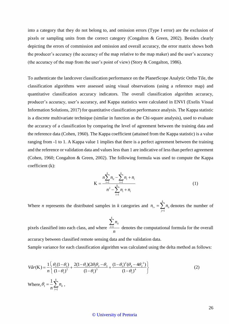
(Cohen, 1960; Congalton & Green, 2002). The following formula was used to compute the Kappa

coefficient (k):

1 1

2

1

k k

ii i i

i i

k

i i

i

n n n n

n n n

(1)

Where n represents the distributed samples in k categories and 1

k

i ii

j

n n

denotes the number of

pixels classified into each class, and where 1

k

ii

i

n

n

denotes the computational formula for the overall

accuracy between classified remote sensing data and the validation data.

Sample variance for each classification algorithm was calculated using the delta method as follows:

2 2

1 1 2 31 1 1 4 2

2 3 4

1 1 1

2(1 )(2(1 ) (1 ) ( 4 )1( )

(1 ) (1 ) (1 )Vâr

n

(2)

Where, 1

1

1 k

ii

i

nn

,


27

2 21

1 k

i i

i

n nn

,

3 21

1( )

k

ii i i

i

n n nn

,

and

2

4 31 1

1( )

k k

ij j i

i i

n n nn

,

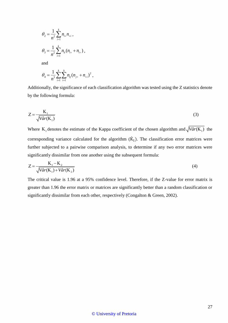
Additionally, the significance of each classification algorithm was tested using the Z statistics denote

by the following formula:

1

1)(ˆVar

(3)

Where 1 denotes the estimate of the Kappa coefficient of the chosen algorithm and 1(ˆ )Var the

corresponding variance calculated for the algorithm (Ḱ1). The classification error matrices were

further subjected to a pairwise comparison analysis, to determine if any two error matrices were

significantly dissimilar from one another using the subsequent formula:

1 2

1 2ˆ ˆ) )( (Var Var

(4)

The critical value is 1.96 at a 95% confidence level. Therefore, if the Z-value for error matrix is

greater than 1.96 the error matrix or matrices are significantly better than a random classification or

significantly dissimilar from each other, respectively (Congalton & Green, 2002).


28

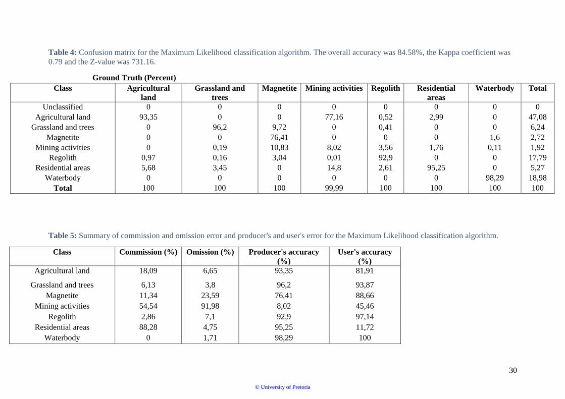
Chapter 4: Results

Common and advanced algorithms were used to classify satellite imagery of the Eastern Limb of the

Bushveld Complex and to detect and map magnetite. Tables 4 to 11 illustrate the confusion matrix of

common or traditional and advanced classification algorithms and their respective accuracies and

errors. Figures 7 to 10 convey the landcover classification of the seven classes using the different

algorithms. Each is depicted in a different colour. Magnetite is depicted in dark shade of blue in all

the classification algorithms.

4.1 Evaluating the performance of the classification algorithms

In this section we computed the confusion matrix for all the classification algorithms discussed, using

a total of 120 AOIs points for the PlanetScope Ortho-tile image. The user’s accuracy is an indicator

of how well the training data was accurately distinguished. On the other hand, the producer’s accuracy

is an indicator of the model’s ability to predict itself. In the case of the Maximum Likelihood

classification algorithm, the algorithm that had the highest accuracy (Table 4 and Figure 7) conveyed

a clearer distinction between classes compared to the mixture of classes noted in Figures 8, 9 & 10.

Irrespective of the Maximum Likelihood classification algorithm illustrating better class

categorization, a large proportion of the mining activity pixels were incorrectly classified as

agricultural land (Table 4). However, this observation was not merely limited to the Maximum

Likelihood classification algorithm, but to all image classifications (Minimum Distance to Means,

Artificial Neural Network, and Support Vector Machine classification algorithms (Table 6, 8 & 10)).

Statistical analyses revealed that the four classification algorithms performed better than a random

classification, with each classification attaining a Z-value significantly higher than 1.96 at a 95%

confidence level. The commission errors for mining activities (Table 5, 7, 9 & 11) were higher in all

the discussed classified algorithms, indicating misclassifications for the class. This is an indication of

the similarity in the spectral reflectance of mining activities and agricultural land. Agricultural land,

water bodies, and grassland and trees were seldom misclassified in the thematic maps.

The pairwise comparison test performed using the error matrices of the classification algorithms

indicated that the Maximum Likelihood classification algorithm was the most significantly different.

The Maximum Likelihood classification algorithm’s producer’s accuracy was higher than all the

other classification algorithms for magnetite, with its prediction percentage of 76.41. Additionally,

the algorithm was able to accurately distinguish magnetite 88.66% of the time. This indicates that

magnetite can be identified with a high level of accuracy. Most notably, the Minimum Distance to


29

Means, Artificial Neural Network, and Support Vector Machine classification algorithms had a higher

commission and omission errors for magnetite (Table 7, 9 & 11), indicating the algorithms’ inability

to accurately classify magnetite. From the results in Tables 3 and 9, it is understood that the Maximum

Likelihood and Support Vector Machine- based classification algorithms are the two supervised

algorithms that give the most accurate overall classification accuracy. In terms, of its ability to predict

magnetite, the Minimum Distance to Means classification algorithm was ranked as second best with

prediction accuracy of 42.15% and a low ability to distinguish magnetite (18.20%).

The Minimum Distance to Means and Support Vector classification algorithms were accurate in

classifying most water bodies, residential areas, and grassland and trees, as is evident from Table 6

& 10 and Figures 8 & 10. The main difference between the Maximum Likelihood (Figure 7) and

Minimum Distance to Means (Figure 8) classification landcover map is the large proportion of the

landscape that is classified as regolith, which almost completely envelops areas that are agricultural

land, grassland and trees, mining areas, and residential areas, in the Minimum Distance to Means

classification. The Minimum Distance to Means and Support Vector classification algorithms, on the

other hand, classified some portions of grassland and trees as mining areas. Subsequently, the

Minimum Distance to Means and the Support Vector classification algorithms have some more errors

of commission and errors of omission than the Maximum Likelihood classification algorithm, evident

from Tables 4, 6 & 10. Similar to both Minimum Distance to Means and the Support Vector

classification algorithms, the Artificial Neural Network classification algorithm illustrated a

landscape disproportionally classified by one or two landcover classes, in this case, agriculture and

grassland and trees. This inadvertently gave the two classes a false high accuracy.


30

Table 4: Confusion matrix for the Maximum Likelihood classification algorithm. The overall accuracy was 84.58%, the Kappa coefficient was

0.79 and the Z-value was 731.16.

Ground Truth (Percent)

Class Agricultural

land

Grassland and

trees

Magnetite Mining activities Regolith Residential

areas

Waterbody Total

Unclassified 0 0 0 0 0 0 0 0

Agricultural land 93,35 0 0 77,16 0,52 2,99 0 47,08

Grassland and trees 0 96,2 9,72 0 0,41 0 0 6,24

Magnetite 0 0 76,41 0 0 0 1,6 2,72

Mining activities 0 0,19 10,83 8,02 3,56 1,76 0,11 1,92

Regolith 0,97 0,16 3,04 0,01 92,9 0 0 17,79

Residential areas 5,68 3,45 0 14,8 2,61 95,25 0 5,27

Waterbody 0 0 0 0 0 0 98,29 18,98

Total 100 100 100 99,99 100 100 100 100

Table 5: Summary of commission and omission error and producer's and user's error for the Maximum Likelihood classification algorithm.

Class Commission (%) Omission (%) Producer's accuracy

(%)

User's accuracy

(%)

Agricultural land 18,09 6,65 93,35 81,91

Grassland and trees 6,13 3,8 96,2 93,87

Magnetite 11,34 23,59 76,41 88,66

Mining activities 54,54 91,98 8,02 45,46

Regolith 2,86 7,1 92,9 97,14

Residential areas 88,28 4,75 95,25 11,72

Waterbody 0 1,71 98,29 100


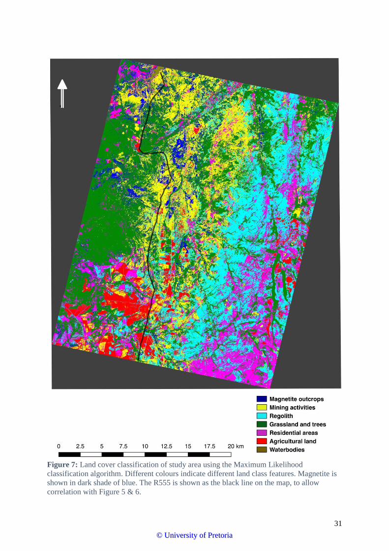
31

Figure 7: Land cover classification of study area using the Maximum Likelihood

classification algorithm. Different colours indicate different land class features. Magnetite is

shown in dark shade of blue. The R555 is shown as the black line on the map, to allow

correlation with Figure 5 & 6.


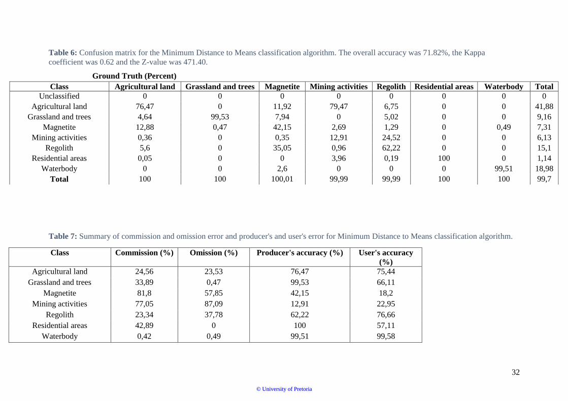
32

Table 6: Confusion matrix for the Minimum Distance to Means classification algorithm. The overall accuracy was 71.82%, the Kappa

coefficient was 0.62 and the Z-value was 471.40.

Table 7: Summary of commission and omission error and producer's and user's error for Minimum Distance to Means classification algorithm.

Class Commission (%) Omission (%) Producer's accuracy (%) User's accuracy

(%)


Grassland and trees 33,89 0,47 99,53 66,11

Magnetite 81,8 57,85 42,15 18,2


Regolith 23,34 37,78 62,22 76,66

Residential areas 42,89 0 100 57,11

Waterbody 0,42 0,49 99,51 99,58


Class Agricultural land Grassland and trees Magnetite Mining activities Regolith Residential areas Waterbody Total


Agricultural land 76,47 0 11,92 79,47 6,75 0 0 41,88

Grassland and trees 4,64 99,53 7,94 0 5,02 0 0 9,16

Magnetite 12,88 0,47 42,15 2,69 1,29 0 0,49 7,31

Mining activities 0,36 0 0,35 12,91 24,52 0 0 6,13

Regolith 5,6 0 35,05 0,96 62,22 0 0 15,1

Residential areas 0,05 0 0 3,96 0,19 100 0 1,14

Waterbody 0 0 2,6 0 0 0 99,51 18,98

Total 100 100 100,01 99,99 99,99 100 100 99,7


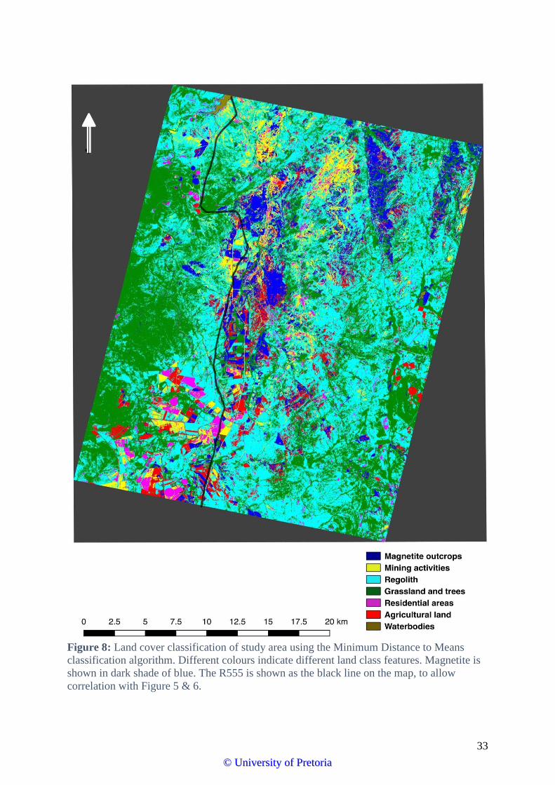
33

Figure 8: Land cover classification of study area using the Minimum Distance to Means





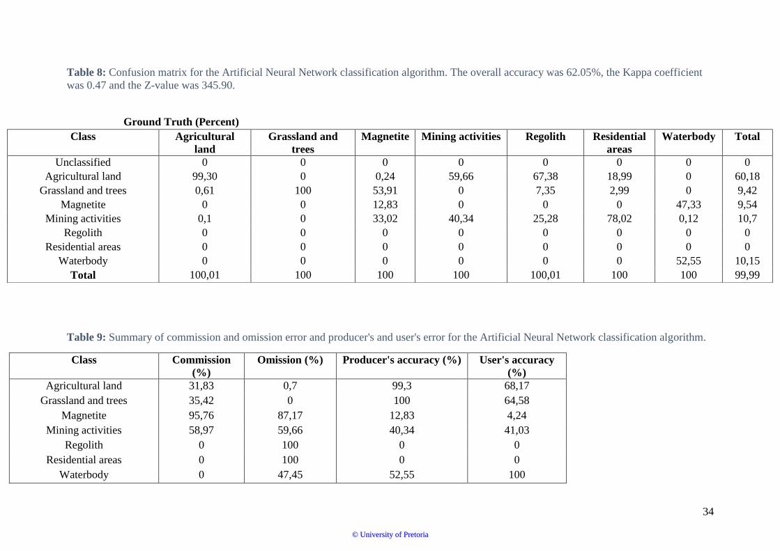
34

Table 8: Confusion matrix for the Artificial Neural Network classification algorithm. The overall accuracy was 62.05%, the Kappa coefficient

was 0.47 and the Z-value was 345.90.

Table 9: Summary of commission and omission error and producer's and user's error for the Artificial Neural Network classification algorithm.

Class Commission

(%)

Omission (%) Producer's accuracy (%) User's accuracy

(%)


Grassland and trees 35,42 0 100 64,58

Magnetite 95,76 87,17 12,83 4,24


Regolith 0 100 0 0

Residential areas 0 100 0 0

Waterbody 0 47,45 52,55 100


Class Agricultural

land

Grassland and

trees

Magnetite Mining activities Regolith Residential

areas

Waterbody Total


Agricultural land 99,30 0 0,24 59,66 67,38 18,99 0 60,18

Grassland and trees 0,61 100 53,91 0 7,35 2,99 0 9,42

Magnetite 0 0 12,83 0 0 0 47,33 9,54

Mining activities 0,1 0 33,02 40,34 25,28 78,02 0,12 10,7

Regolith 0 0 0 0 0 0 0 0

Residential areas 0 0 0 0 0 0 0 0

Waterbody 0 0 0 0 0 0 52,55 10,15

Total 100,01 100 100 100 100,01 100 100 99,99


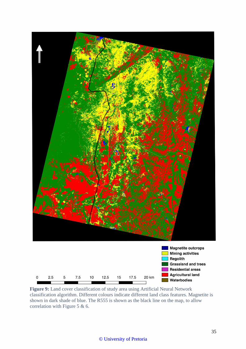
35

Figure 9: Land cover classification of study area using Artificial Neural Network





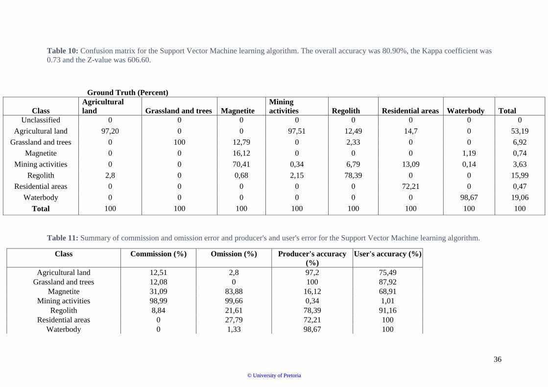
36

Table 10: Confusion matrix for the Support Vector Machine learning algorithm. The overall accuracy was 80.90%, the Kappa coefficient was

0.73 and the Z-value was 606.60.

Table 11: Summary of commission and omission error and producer's and user's error for the Support Vector Machine learning algorithm.


Class

Agricultural

land Grassland and trees Magnetite

Mining

activities Regolith Residential areas Waterbody Total


Agricultural land 97,20 0 0 97,51 12,49 14,7 0 53,19

Grassland and trees 0 100 12,79 0 2,33 0 0 6,92

Magnetite 0 0 16,12 0 0 0 1,19 0,74

Mining activities 0 0 70,41 0,34 6,79 13,09 0,14 3,63

Regolith 2,8 0 0,68 2,15 78,39 0 0 15,99

Residential areas 0 0 0 0 0 72,21 0 0,47

Waterbody 0 0 0 0 0 0 98,67 19,06

Total 100 100 100 100 100 100 100 100

Class Commission (%) Omission (%) Producer's accuracy

(%)

User's accuracy (%)


Grassland and trees 12,08 0 100 87,92

Magnetite 31,09 83,88 16,12 68,91


Regolith 8,84 21,61 78,39 91,16

Residential areas 0 27,79 72,21 100

Waterbody 0 1,33 98,67 100


37

Figure 10: Land cover classification of study area using Support Vector Machine learning

algorithm. Different colours indicate different land class features. Magnetite is shown in dark

shade of blue. The R555 is shown as the black line on the map, to allow correlation with

Figure 5 & 6.


38

Chapter 5: Discussion

Although multispectral and hyperspectral imagery are two widely used components of remote

sensing for lithological discrimination and classification, obtaining appropriate hyperspectral

imagery for mineral and geological mapping is challenging because of the high costs and

intricacy of the treatment associated with hyperspectral remote sensing (Ge et al., 2018).

Hence, the amalgamation of high spatial multispectral remote sensing data with reliable

textural and reference data is very effective in attaining useful results.

This project aimed to map magnetite bodies using common and advanced classification

algorithms on the Upper Zone of the Eastern Limb of the RLS and to compare and contrast the

performance of common classification algorithms over the advanced classification algorithms.

We had expected advanced classification algorithms to be better equipped than common

traditional classification algorithms for the detection and mapping of magnetite owing to the

algorithms’ advanced data analysis tools, and to depict a more realistic classification of the

different classes.

Of the four classification algorithms outputs accuracies evaluated in this study, the Maximum

Likelihood classification algorithm performed best in the overall prediction accuracy of all

seven classes (with an overall accuracy of 84.58%) and was the algorithm most fit for the

detection and mapping of magnetite (with a producer’s accuracy of 76.41% and a user’s

accuracy of 88.66%) in the Eastern Limb of the Bushveld Complex. The result was not in

accordance to the expectations of the study; additionally this result was in contrast to other

studies that had compared the performance of common and advanced classification algorithms

(Pal & Mather, 2005; Joevivek & Chandrasekar, 2010; Otukei & Blaschke, 2010; Yu et al.,

2012; Omeer et al., 2018). The aforementioned studies found that advanced classification

algorithms (Support Vector Machines and Artificial Neural Networks) better performed and

provided higher accuracies than common traditional classification algorithms (Maximum

Likelihood and Minimum Distance to Means classification algorithm) in terms of classifying

independent validated classes or landcover categories.

Though the other three algorithms (Minimum Distance to Means, Artificial Neural Networks,

and Support Vector Machines) did not yield acceptably accurate results for the detection of

magnetite, their overall accuracies were unexpectedly high. There are two plausible factors that


39

may have accounted for the high overall accuracy levels in all three classification algorithms

in this study. First, and the most noteworthy, is the prevalence of extensive and easily

differentiable classes (e.g. grassland trees, agricultural area, and waterbodies), which

indubitably contributed to the consistently high overall accuracies. The spatial limitation of the

other classes relative to the aforementioned classes with a greater spatial capacity (i.e.

grassland and trees, agricultural areas, and waterbodies) contributed to a high overall

performance values or scores by curbing both the amount and spectral diversity of the pixels

belonging to the spatially constrained classes (e.g. mining areas, residential areas and

magnetite). The later mentioned factor likely led to the overfitting of certain other classes noted

in Figures 8 & 9. Lastly, single developed classes were used in this study, which encompassed

some landcover pixels being categorized as residential areas, despite including roads and other

non-residential buildings.

The Maximum Likelihood and the Support Vector Machine classification algorithms were the

only algorithms with a Kappa value above 70%, with both achieving an overall accuracy of

over 80%, which is an impressive result according to (Foody, 2008). However, it must be noted

that the overall accuracy of the Support Vector Machine classification algorithm was relatively

higher than the other classification algorithms (apart from the Maximum Likelihood

classification algorithm), owing to the fact that the majority of non-geological classes with the

highest number of pixels were the pixels that had the highest accuracies (e.g. agricultural land,

water bodies, regolith, and grassland trees). Since the overall accuracy formula is based on the

number of pixels of each class, classes with a high pixel count are likely to positively skew the

overall accuracy. In fact, with the high pixel count classes removed, the Support Vector

Machine classification algorithm has a comparatively small overall accuracy of 20.95%. In

comparison, with the removal of the non-geological classes, the Maximum Likelihood

classification algorithm attained an overall accuracy of 64.35%. Szuster et al. (2011) found the

Support Vector Machine classification algorithm to be the best classification algorithm for

separating man-made infrastructures from those of nature, irrespective of the similarity in

spectral signatures. The simplification of the different validated classes or landcover categories

in Support Vector Machines classification algorithms, should have made it easier to develop

hyperplanes and therefore to detect and discriminate the different classes.


40

Despite prior successes in lithological mapping, Support Vector Machine and Artificial Neural

Network classification algorithms were not able to accurately detect exposed magnetite bodies

in this study. This may have been in part due to the spectral resolution of the imagery, the

heterogeneity of the chemical mineralogical composition of the mining areas at the sub-pixel

level, and algorithm high bias (when algorithms are underfitted, i.e. not having enough features

for the target outputs). However, high bias algorithms do not benefit from more training data,

but, they may benefit from more features or training data. The heterogeneity of chemical

composition may have affected the resultant spectral purity of magnetite through the intimate

or non-linear spectral combination of the spectra of end-members (Gupta, 2017). Other mineral

or oxides (such hematite and limonite) found in association with weathered magnetite in

magnetite bodies, may have contaminated the spectral response of magnetite, causing it to be

correlated with the absorption bands of hematite and limonite.

As previously found by Hunt (1971), the increase in the size of magnetite grains equates to an

increase in the reflectance of incident photons of light and absorption features. The different

spectral signature of magnetite, owing to an increase in spectral reflectance may have led to

some magnetite bodies being misclassified. Regardless of the rigorous pre-processing, the

above-mentioned factors could have affected the spectral responses of the magnetite bodies.

The aforementioned shortcomings are a result of using a sensor with 4-bands, which has broad

wavelength ranges and therefore makes it difficult to distinguish the finer absorption

characteristics of magnetite bodies. However, this was due to the trade-offs between spatial,

spectral, and radiometric resolution of the sensor that was chosen and was a better fit for the

this undertaking. Hence, a sensor with a high or finer spectral resolution is essential when

absorption lines of various geological features are located in the same spectral range with other

geological features that interfere with each other. Using sensors with finer spectral resolutions

(sensors with narrower band widths) creates the opportunity to identify some materials by

their absorption-band characteristics (i.e. accurately discriminate some of the features that

make up the remote sensing signal) and attenuate the interference.

The overall high accuracy classification of the Maximum Likelihood classification algorithm

in this study suggests the classification algorithm may be advantageous in the detection and

mapping of exposed magnetite bodies and that remote sensing methods are effective tools for

geological mapping and mineral exploration, especially in iron oxides (despite the other


41

geological features obscuring the spectral reflectance of the focal substrate). Indeed, full

knowledge of the performance differences of each classification algorithm is crucial for the

choice of a classification algorithm for a particular scene and application. As with numerous

remote sensing applications, the greater onus should be placed on the precision and accuracy

of the dataset than the classification algorithms used for analysis. Although, the choice of

classification algorithm will undoubtedly influence the success of mineral detection and

mapping, the accessibility, quality, and processing of geology data will have an even greater

impact on the results. This includes the size of the study area and the spatial and spectral

resolution of the data. In essence, the choice of the most appropriate algorithm should be based

on the characteristics of the data, as well as, the research objectives.


42

Chapter 6: Recommendations and conclusion

The present study focused on the remote sensing capability to map the lithological occurrence

of magnetite bodies with the help of geographical information system (GIS) on the Eastern

Limb of the Bushveld Complex. Although numerous studies have detected the lithological

occurrence of ore oxides using remote sensing, very few studies have detected the lithological

occurrence of the opaque mineral, magnetite (Rajendran et al., 2007; Raja et al., 2010; Izawa

et al., 2019), and none have explored the occurrence of magnetite in the Bushveld Complex.

This study revealed that the lithological occurrence of magnetite could be successfully detected

with a satisfactory level of success, using the common traditional classification algorithms,

Maximum Likelihood. The results attained from the Maximum Likelihood classification

algorithm indicated that the producer’s and user’s accuracies were 76.41% and 88.66%,

respectively. The computed kappa coefficient was 0.79, illustrating a high categorical and

overall accuracy. The thematic map derived from the Maximum Likelihood classification

algorithm had an overall accuracy of 84.58%.

Despite the success of this study, some improvements could be made. Naturally, the type and

size of data of the training data affect the accuracy of classification algorithms. In particular,

with the Artificial Neural Network and Support Vector classification algorithms, for better

performance, a larger data size was required. This lack of a more robust dataset may have

introduced potential omission and commission errors in the results. Furthermore, to improve

the accuracy of the classification algorithms, using a fuzzy membership function is

recommended. Using a fuzzy membership function will objectively classify pixels to their

correct end-member class (Moore et al., 2001; Malik et al., 2013).

Spectral mixing was an unavoidable challenge in the lithological discrimination and mapping

of magnetite. Since magnetite was predominately found in medium to densely vegetated areas

(dominated by Senecio microglossus), the magnetite spectral signature was often mixed with

that of vegetation. Since this signature could not be removed from the PlanetScope image,

Campbell (1996) suggested the exploitation of plants through geobotany. Geobotany rests on

the absorption of elements, released by geological material in the soil, by the plants. With the

use of remote sensing, the recorded signatures of the elements within the plants could be used

to infer the underlying geology. Although feasible, the idea has a few restrictions but is still a

worthwhile research path. Furthermore, this study mainly investigated the lithological accuracy


43

of detecting magnetite, however it did not consider the underlying stratigraphy of the magnetite

bodies using geophysics. Therefore, a future line of investigations could assess the underlying

stratigraphy to determine whether or not magnetite bodies exhibit a similar ‘carrot-shaped’

intrusion as kimberlites.

Although the imagery used for this study had a high spatial resolution, the drawbacks of a four-

band sensor were noted. Spectral information was lost through the bands of the PlanetScope

product. Hence, there is a great amount of spectral information to be gained from using 220

bands found in hyperspectral remote sensing, though the products are very expensive and

obtaining appropriate hyperspectral imagery for mineral and geological mapping is difficult,

the conceptual performance characteristics over multispectral remote sensing are better.

For future research, it may be beneficial and of value to perform supplementary analyses on

the same area over different times using the same data source to confirm the results attained in

this study. This would, of course, convey whether the findings noted in this study were solely

a result of the performance of the Maximum Likelihood classification algorithm as opposed to

either imagery error and or random data noise.

Overall this study suggests the relevance and efficiency of using the common traditional

classification algorithm – Maximum Likelihood over the advanced classification algorithms –

Support Vector Machine, especially for studies with relatively small datasets. And despite the

accuracy of common traditional classification algorithms and advanced classification

algorithms, it is worth noting that remote sensing and GIS should not solely be used as decision-

making tools or replacements for direct fieldwork but should be amalgamated with different

datasets and the knowledge of a specialist.


44

References

Abrams, M. J., Brown, D., Lepley, L., & Sadowski, R. (1983). Remote sensing for porphyry

copper deposits in southern Arizona. Economic Geology, 78(4), 591-604.

Abulghasem, Y. A., Akhir, J. M., Samsudin, A. R., Hassan, W. F. W., & Youshah, B. M.

(2011). Integrated data of remote sensing and geophysical data for iron ore exploration

in the western part of Wadi Shatti District, Libya. Electronic Journal of Geotechnical

Engineering, 16, 1441-1454.

Agar, B., & Coulter, D. (2007). Remote sensing for mineral exploration–A decade perspective

1997-2007. Paper presented at the Proceedings of Exploration.

Al-Ahmadi, F., & Hames, A. (2009). Comparison of four classification methods to extract land

use and land cover from raw satellite images for some remote arid areas, kingdom of

Saudi Arabia. Earth, 20(1), 167-191.

An, P., Chung, C.-J. F., & Rencz, A. N. (1994). A preliminary study of alteration mapping

from airborne geophysical and remote sensing data using feed-forward neural

networks Paper presented at the 64th Annual International Meeting; Technical Program

Abstracts.

Babakan, S., & Oskouei, M. M. (2014). Integrated use of multispectral remote sensing and GIS

for primary gold favorability mapping in Lahroud Region (NW Iran). Journal of Tethys,

2(3), 228-241.

Bachri, I., Hakdaoui, M., Raji, M., Teodoro, A. C., & Benbouziane, A. (2019). Machine

Learning Algorithms for Automatic Lithological Mapping Using Remote Sensing Data:

A Case Study from Souk Arbaa Sahel, Sidi Ifni Inlier, Western Anti-Atlas, Morocco.

ISPRS International Journal of Geo-Information, 8(6), 248.

Brown, W. M., Gedeon, T., Groves, D., & Barnes, R. (2000). Artificial neural networks: a new

method for mineral prospectivity mapping. Australian journal of earth sciences, 47(4),

757-770.

Campbell, J. B., & Wynne, R. H. (2011). Introduction to remote sensing (Vol. 5). United States

of America, New York: Guilford Press.

Cawthorn, R. (1994). Growth nodes at the base of magnetitite layers in the Upper Zone of the

Bushveld Complex. South African Journal of Geology, 97(4), 455-461.

Cawthorn, R.G. (2010). The platinum group element deposits of the Bushveld Complex South

Africa. Platinum Metals Review, 54(4), pp.205-215.

Cheney, E. S., & Twist, D. (1991). The conformable emplacement of the Bushveld mafic rocks

along a regional unconformity in the Transvaal succession of South Africa.

Precambrian Research, 52(1-2), 115-132.

Chien, Y. (1974). Pattern classification and scene analysis. IEEE Transactions on Automatic

Control, 19(4), 462-463.


45

Chistyakova, S., Latypov, R., & Youlton, K. (2019). Multiple Merensky Reef of the Bushveld

Complex, South Africa. Contributions to Mineralogy and Petrology, 174, 3-26.

Ciampalini, A., Garfagnoli, F., Del Ventisette, C., & Moretti, S. (2013). Potential use of remote

sensing techniques for exploration of iron deposits in Western Sahara and Southwest

of Algeria. Natural Resources Research, 22(3), 179-190.

Cihlar, J. (2000). Land cover mapping of large areas from satellites: status and research

priorities. International Journal of Remote Sensing, 21(6-7), 1093-1114.

Clark, R. N., & Roush, T. L. (1984). Reflectance spectroscopy: Quantitative analysis

techniques for remote sensing applications. Journal of Geophysical Research: Solid

Earth, 89(B7), 6329-6340.

Cloutis, E. A. (1996). Review article hyperspectral geological remote sensing: evaluation of

analytical techniques. International Journal of Remote Sensing, 17(12), 2215-2242.

Cloutis, E. A., McCormack, K. A., Bell III, J. F., Hendrix, A. R., Bailey, D. T., Craig, M. A., .

. . Riner, M. A. (2008). Ultraviolet spectral reflectance properties of common planetary

minerals. Icarus, 197(1), 321-347.

Cohen, J. (1960). A coefficient of agreement for nominal scales. Educational and

psychological measurement, 20(1), 37-46.

Combe, J. P., Launeau, P., Pinet, P., Despan, D., Harris, E., Ceuleneer, G., & Sotin, C. (2006).

Mapping of an ophiolite complex by high‐ resolution visible‐ infrared spectrometry.

Geochemistry, Geophysics, Geosystems, 7(8).

Congalton, R. G. (2001). Accuracy assessment and validation of remotely sensed and other

spatial information. International Journal of Wildland Fire, 10(4), 321-328.

Congalton, R. G., & Green, K. (2002). Assessing the accuracy of remotely sensed data:

principles and practices (Vol. 2). United States of America, New York: CRC press.

Congalton, R. G., Oderwald, R. G., & Mead, R. A. (1983). Assessing Landsat classification

accuracy using discrete multivariate analysis statistical techniques. Photogrammetric

engineering and remote sensing, 49(12), 1671-1678.

Continuum Analytics. (2019). Anaconda Python (Version Python 3.7 version). Retrieved

from https://www.anaconda.com/distribution/

Dare, S. A., Barnes, S.-J., Beaudoin, G., Méric, J., Boutroy, E., & Potvin-Doucet, C. (2014).

Trace elements in magnetite as petrogenetic indicators. Mineralium Deposita, 49(7),

785-796.

Drury, S. A. (2001). Image interpretation in geology (Vol. 3). United Kingdom, Cheltenham:

Chapman & Hall.

Eales, H. V., & Cawthorn, R. G. (1996). The Bushveld Complex (Vol. 15). Netherlands,

Amsterdam: Elsevier.

ERDAS. (2005). ERDAS field guide. Copyright Leica Geosystems Geospatial Imaging, LLC.


https://www.anaconda.com/distribution/

46

Exelis Visual Information Solutions. (2017). Environment for visualizing images. In: Exelis

Visual Information Solutions

Fatima, K., Khattak, U. K., & Kausar, A. B. (2013). Selection of appropriate classification

technique for lithological mapping of Gali Jagir area, Pakistan. Int. J. Earth Sci. Eng,

7(12), 964-971.

Fischer, L. A., Wang, M., Charlier, B., Namur, O., Roberts, R. J., Veksler, I. V., . . . Holtz, F.

(2016). Immiscible iron-and silica-rich liquids in the Upper Zone of the Bushveld

Complex. Earth and Planetary Science Letters, 443, 108-117.

Foody, G. M. (1996). Approaches for the production and evaluation of fuzzy land cover

classifications from remotely-sensed data. International Journal of Remote Sensing,

17(7), 1317-1340.

Foody, G. M. (2008). Harshness in image classification accuracy assessment. International

Journal of Remote Sensing, 29(11), 3137-3158.

Foody, G. M., Campbell, N. A., Trodd, N. M., & Wood, T. F. (1992). Derivation and

applications of probabilistic measures of class membership from the maximum-

likelihood classification. Photogrammetric engineering and remote sensing, 58(9),

1335-1341.

Ge, W., Cheng, Q., Tang, Y., Jing, L., & Gao, C. (2018). Lithological classification using

sentinel-2A data in the Shibanjing ophiolite complex in inner Mongolia, China. Remote

Sensing, 10(4), 638.

Gilles, B., EL-Hihi, S., & Jebrak, M. (1992). Applications of neural network computing to

mining exploration in the southern Abitibi Green-stone Belt. Anonymous GAC7AGC-

MAC AMC. Paper presented at the Joint Annual Meeting.

Google Earth (Cartographer). (2018). Roossenekal -25.193722, 29.924991, elevation

2253.996m. 3D map. Retrieved from

https://www.google.com/maps/place/Roossenekal/data=!4m2!3m1!1s0x1ec1e58802a

9a6dd:0x48d693c133d31ee9?sa=X&ved=2ahUKEwiqmqegjeLjAhXWSxUIHT8xAC

UQ8gEwD3oECAsQBA

Grant , R. C. (2015). The Bushveld Complex, South Africa (Vol. 1). Netherlands, Dordrecht:

Springer Science.

Gupta, R. P. (2017). Remote sensing geology (3rd ed. Vol. 3). Germany, Berlin: Springer-

Verlag.

Gurov, E., Shekhunova, S., & Permyakov, V. (2015). Accessory and opaque minerals in impact

melt rocks of the Boltysh structure, Ukraine. Meteoritics & Planetary Science, 50(6),

1139-1155.

Gurugnanam, B., Arulbalaji, P., Midhuna, V., & Kumaravel, S. (2017). Lithological

Discrimination of Anorthosite using ASTER data in Oddanchatram Area, Dindigul

district, Tamil Nadu, India. International Journal of Advanced Engineering,

Management and Science, 3(4), 9.


https://www.google.com/maps/place/Roossenekal/data=!4m2!3m1!1s0x1ec1e58802a9a6dd:0x48d693c133d31ee9?sa=X&ved=2ahUKEwiqmqegjeLjAhXWSxUIHT8xACUQ8gEwD3oECAsQBA



47

Harmer, R., & Armstrong, R. (2000). New precise dates on the acid phase of the Bushveld and

their implications. Paper presented at the Workshop on the Bushveld Complex,

University of the Witwatersrand, Johannesburg, South Africa.

Harne, D. M., & Von Gruenewaldt, G. (1995). Ore-forming processes in the upper part of the

Bushveld complex, South Africa. Journal of African Earth Sciences, 20(2), 77-89.

Haykin, S. (1994). Neural networks: a comprehensive foundation (Vol. 2). United States, New

Jersey: Prentice Hall.

Healey, G., & Slater, D. (1999). Models and methods for automated material identification in

hyperspectral imagery acquired under unknown illumination and atmospheric

conditions. IEEE Transactions on geoscience and remote sensing, 37(6), 2706-2717.

Herold, M., Mayaux, P., Woodcock, C., Baccini, A., & Schmullius, C. (2008). Some challenges

in global land cover mapping: An assessment of agreement and accuracy in existing 1

km datasets. Remote Sensing of Environment, 112(5), 2538-2556.

Hunt, G. R. (1971). Visible and near-infrared spectra of minerals and rocks: III. Oxides and

hydro-oxides. Modern Geology, 2, 195-205.

Impala Platinum. (2014). Mineral resource and mineral reserve statement. Annual Report.

Inzana, J., Kusky, T., Higgs, G., & Tucker, R. (2003). Supervised classifications of Landsat

TM band ratio images and Landsat TM band ratio image with radar for geological

interpretations of central Madagascar. Journal of African Earth Sciences, 37(1-2), 59-

72.

Izawa, M. R., Cloutis, E. A., Rhind, T., Mertzman, S. A., Applin, D. M., Stromberg, J. M., &

Sherman, D. M. (2019). Spectral reflectance properties of magnetites: Implications for

remote sensing. Icarus, 319, 525-539.

Jensen, J. R. (2005). Introductory digital image processing: a remote sensing perspective (Vol.

2). United States of America, New Jersey: Prentice Hall

Jia, K., Wu, B., Tian, Y., Zeng, Y., & Li, Q. (2011). Vegetation classification method with

biochemical composition estimated from remote sensing data. International Journal of

Remote Sensing, 32(24), 9307-9325.

Joevivek, V., & Chandrasekar, N. (2010). Comparison of Supervised Classification Methods

for Efficiently Locating Possible Mineral Deposits using Multispectral Remote Sensing

data. International Journal of Advanced Research in Computer Science, 1(3).

Joseph, A., & Bamidele, O. (2018). Application of remote sensing method for geological

interpretation of Sokoto Plain, Nigeria. South African Journal of Geomatics, 7(3), 360-

371.

Kavzoglu, T., & Colkesen, I. (2009). A kernel functions analysis for support vector machines

for land cover classification. International Journal of Applied Earth Observation and

Geoinformation, 11(5), 352-359.


48

Kavzoglu, T., & Reis, S. (2008). Performance analysis of maximum likelihood and artificial

neural network classifiers for training sets with mixed pixels. GIScience & Remote

Sensing, 45(3), 330-342.

Kemp, J. N., Zietsman, H. L., & Stevens, G. (2005). Evaluating image classification techniques

on Aster data for lithological discrimination in the Barberton Greenstone Belt,

Mpumalanga, South Africa. (Master of Science), University of Stellenbosch,

Stellenbosch.

Kim, H., & Pang, S. (2003). Automatic land cover analysis for Tenerife by supervised

classification using remote sensing data. Remote Sensing of the Environment, 86, 530-

541.

Kinnaird, J. A. (2005). The Bushveld large igneous province. Review Paper, The University of

the Witwatersrand, Johannesburg, South Africa, 39pp.

Klemm, D., Henckel, J., Dehm, R., & Von Gruenewaldt, G. (1985). The geochemistry of

titanomagnetite in magnetite layers and their host rocks of the eastern Bushveld

Complex. Economic Geology, 80(4), 1075-1088.

Legodi, M. A., & de Waal, D. (2007). The preparation of magnetite, goethite, hematite and

maghemite of pigment quality from mill scale iron waste. Dyes and Pigments, 74(1),

161-168.

Li, J. Q., Yi, H., Ren, G. L., Gao, T., Yang, M., Han, H. H., & Yang, J. L. (2016). High

resolution remote sensing and potential analysis of iron ore prospecting——Taking

Datong Township, West KunLun Area for example. Paper presented at the IOP

Conference Series: Earth and Environmental Science.

Lillesand, T. M., & Kiefer, R. W. (2000). Remote Sensing and Image Interpretation (Vol. 4).

United States of America, New Jersey: John Wiley & Sons.

Low, A. B., & Rebelo, A. G. (1998). Vegetation of South Africa, Lesotho and Swaziland: A

companion to the vegetation map of South Africa, Lesotho and Swaziland.

Maila, R. P. (2015). Geochemistry of magnetite layers in the upper zone of the Bushveld

Complex, South Africa. (Master's Dissertation), WITS University, South Africa.

Malik, V., Gautam, A., Sahai, A., Jha, A., & Singh, A. (2013). Satellite Image Classification

Using Fuzzy Logic. International Journal of Recent Technology and Engineering

(IJRTE), 2(2), 204-207.

Manuel, R., Brito, M., Chichorro, M., & Rosa, C. (2017). Remote sensing for mineral

exploration in central Portugal. Minerals, 7(10), 184.

Marapareddy, R., Aanstoos, J., & Younan, N. (2017). Accuracy Analysis Comparison of

Supervised Classification Methods for Anomaly Detection on Levees Using SAR

Imagery. Electronics, 6(4), 83.

Martins, A. K., & Gadiga, B. L. (2015). Satellite Remote Sensing for Mineral Deposit

Assessment of Clay in Mubi Local Government Area of Adamawa State, Nigeria.

Geosciences, 5(1), 26-30.


49

Mather, P., & Tso, B. (2016). Classification methods for remotely sensed data (2 ed. Vol. 2).

Unites States of America, Boca Raton: CRC press.

Mather, P. M., & Koch, M. (2011). Computer processing of remotely-sensed images: an

introduction (Vol. 4). United States f America, New Jersey: John Wiley & Sons.

McCarthy, T., Cawthorn, R. G., Wright, C., & McIver, J. (1985). Mineral layering in the

Bushveld Complex; implications of Cr abundances in magnetite from closely spaced

magnetitite and intervening silicate-rich layers. Economic Geology, 80(4), 1062-1074.

Metternicht, G., & Zinck, J. (2003). Remote sensing of soil salinity: potentials and constraints.

Remote Sensing of Environment, 85(1), 1-20.

Mitra, P., Shankar, B. U., & Pal, S. K. (2004). Segmentation of multispectral remote sensing

images using active support vector machines. Pattern recognition letters, 25(9), 1067-

1074.

Molyneux, T. (1974). A geological investigation of the Bushveld Complex in Sekhukhuneland

and part of the Steelpoort valley. South African Journal of Geology, 77(3), 329-338.

Mondal, A., Kundu, S., Chandniha, S. K., Shukla, R., & Mishra, P. (2012). Comparison of

support vector machine and maximum likelihood classification technique using satellite

imagery. International Journal of Remote Sensing and GIS, 1(2), 116-123.

Moore, T. S., Campbell, J. W., & Feng, H. (2001). A fuzzy logic classification scheme for

selecting and blending satellite ocean color algorithms. IEEE Transactions on

geoscience and remote sensing, 39(8), 1764-1776.

Morris, R. V., Lauer Jr, H. V., Lawson, C. A., Gibson Jr, E. K., Nace, G. A., & Stewart, C.

(1985). Spectral and other physicochemical properties of submicron powders of

hematite (α‐ Fe2O3), maghemite (γ‐ Fe2O3), magnetite (Fe3O4), goethite (α‐FeOOH), and lepidocrocite (γ‐ FeOOH). Journal of Geophysical Research: Solid

Earth, 90(B4), 3126-3144.

Murtaza, K. O., & Romshoo, S. A. (2014). Determining the suitability and accuracy of various

statistical algorithms for satellite data classification. International Journal of

Geomatics and Geosciences, 4(4), 585.

Nagy, H., Watanabe, K., & Hirano, M. (2002). Prediction of sediment load concentration in

rivers using artificial neural network model. Journal of Hydraulic Engineering, 128(6),

588-595.

Ngcofe, L., & Van Niekerk, A. (2016). Advances in optical earth observation for geological

mapping: A Review. South African Journal of Geomatics, 5(1), 1-16.

Omeer, A. A., Deshmukh, R. R., Gupta, R. S., & Kayte, J. N. (2018). Land Use and Cover

Mapping Using SVM and MLC Classifiers: A Case Study of Aurangabad City,

Maharashtra, India. Paper presented at the International Conference on Recent Trends

in Image Processing and Pattern Recognition.

Osborne, D. A. (1992). Neural networks provide more accurate reservoir permeability. Oil and

Gas Journal, 90(39).


50

Otukei, J. R., & Blaschke, T. (2010). Land cover change assessment using decision trees,

support vector machines and maximum likelihood classification algorithms.

International Journal of Applied Earth Observation and Geoinformation, 12, S27-S31.

Pal, M., & Mather, P. (2005). Support vector machines for classification in remote sensing.

International Journal of Remote Sensing, 26(5), 1007-1011.

Planet Team (Cartographer). (2018). Planet Application Program Interface: In Space for Life

on Earth. Retrieved from https://api.planet.com

Putra, I., Abbas, R., Masti, S., & Warmada, I. (2018). Remote Sensing Application in

Exploration of Iron Mineral Placer Deposit: Case Study of Kulonprogo's Iron Placer

Deposit. Paper presented at the EAGE-HAGI 1st Asia Pacific Meeting on Near Surface

Geoscience and Engineering.

QGIS Development Team. (2015). QGIS Geographic Information System. Open Source

Geospatial Foundation Project. URL: http://qgis. osgeo. org.

Raja, S., Rajendran, S., Ganesh, P. B., & Thirunavukkarasu, A. (2010). Study on Hyperspectral

Signatures for Magnetite Iron ore in Thattayengerpet region of Trichirappalli district in

Tamil Nadu State, India. International Journal of Geomatics and Geosciences, 1(2),

188.

Rajendran, S., Thirunavukkaraasu, A., Poovalingaganesh, B., Kumar, K. V., & Bhaskaran, G.

(2007). Discrimination of low-grade magnetite ores using remote sensing techniques.

Journal of the Indian Society of Remote Sensing, 35(2), 153.

Rawat, J., Biswas, V., & Kumar, M. (2013). Changes in land use/cover using geospatial

techniques: A case study of Ramnagar town area, district Nainital, Uttarakhand, India.

The Egyptian Journal of Remote Sensing and Space Science, 16(1), 111-117.

Reynolds, I. M. (1985). Contrasted mineralogy and textural relationships in the uppermost

titaniferous magnetite layers of the Bushveld Complex in the Bierkraal area north of

Rustenburg. Economic Geology, 80(4), 1027-1048.

Richards, J. A. (1999). Remote sensing digital image analysis (Vol. 3). Germany, Berlin:

Springer-Verlag.

Rodriguez-Galiano, V., Sanchez-Castillo, M., Chica-Olmo, M., & Chica-Rivas, M. (2015).

Machine learning predictive models for mineral prospectivity: An evaluation of neural

networks, random forest, regression trees and support vector machines. Ore Geology

Reviews, 71, 804-818.

Rokos, D., Argialas, D., Mavrantza, R., Seymour, K. S.-., Vamvoukakis, C., Kouli, M., . . .

Denes, G. (2000). Structural analysis for gold mineralization using remote sensing and

geochemical techniques in a GIS environment: island of Lesvos, Hellas. Natural

Resources Research, 9(4), 277-293.

Rollin, E., Milton, E., & Roche, P. (1994). The influence of weathering and lichen cover on

the reflectance spectra of granitic rocks. Remote Sensing of Environment, 50(2), 194-

199.


https://api.planet.com/

http://qgis/

51

Rowan, L. C., & Mars, J. C. (2003). Lithologic mapping in the Mountain Pass, California area

using advanced spaceborne thermal emission and reflection radiometer (ASTER) data.

Remote Sensing of Environment, 84(3), 350-366.

Rowan, L. C., Mars, J. C., & Simpson, C. J. (2005). Lithologic mapping of the Mordor, NT,

Australia ultramafic complex by using the Advanced Spaceborne Thermal Emission

and Reflection Radiometer (ASTER). Remote Sensing of Environment, 99(1-2), 105-

126.

Rutherford, M. C., Mucina, L., & Powrie, L. W. (2006). Biomes and bioregions of southern

Africa. The vegetation of South Africa, Lesotho and Swaziland, 19, 30-51.

Sabins, F. F. (1999). Remote sensing for mineral exploration. Ore Geology Reviews, 14(3-4),

157-183.

SACS. (1980). Stratigraphy of South Africa (Vol. 1): R & E Publishers.

Schetselaar, E. M., Chung, C.-J. F., & Kim, K. E. (2000). Integration of Landsat TM, gamma-

ray, magnetic, and field data to discriminate lithological units in vegetated. Remote

Sensing of Environment, 71(1), 89-105.

Schouwstra, R., Kinloch, E., & Lee, C. (2000). A short geological review of the Bushveld

Complex. Platinum Metals Review, 44(1), 33-39.

Schulte, R. F., Taylor, R. D., Piatak, N. M., & Seal II, R. R. (2010). Stratiform chromite deposit

model (2331-1258). Retrieved from

Schweitzer, J., Hatton, C., & De Waal, S. (1995). Regional lithochemical stratigraphy of the

Rooiberg Group, upper Transvaal Supergroup: a proposed new subdivision. South

African Journal of Geology, 98(3), 245-255.

Scoon, R., & Mitchell, A. (2012). The Upper Zone of the Bushveld Complex at Roossenekal,

South Africa: geochemical stratigraphy and evidence of multiple episodes of magma

replenishment. South African Journal of Geology, 115(4), 515-534.

Shirazi, A., Hezarkhani, A., Shirazy, A., & Shahrood, I. (2018). Remote Sensing Studies for

Mapping of Iron Oxide Regions, South of Kerman, IRAN. International Journal of

Science and Engineering Applications(04), 45-51.

Siebert, S., Van Wyk, A., Bredenkamp, G., & Mucina, L. (2002a). The physical environment

and major vegetation types of Sekhukhuneland, South Africa. South African Journal of

Botany, 68(2), 127-142.

Siebert, S., Van Wyk, A., Bredenkamp, G., & Mucina, L. (2002b). Vegetation ecology of

Sekhukhuneland, South Africa: Combretum hereroense–Grewia vernicosa Open

Mountain Bushveld. South African Journal of Botany, 68(4), 475-496.

Singer, D. A., & Kouda, R. (1996). Application of a feedforward neural network in the search

for Kuroko deposits in the Hokuroku district, Japan. Mathematical Geology, 28(8),

1017-1023.


52

Singer, D. A., & Kouda, R. (1997a). Classification of mineral deposits into types using

mineralogy with a probabilistic neural network. Nonrenewable Resources, 6(1), 27-32.

Singer, D. A., & Kouda, R. (1997b). Use of a neural network to integrate geoscience

information in the classification of mineral deposits and occurrences. Paper presented

at the Proceedings of exploration.

Soe, M., Kyaw, T. A., & Takashima, I. (2005). Application of remote sensing techniques on

iron oxide detection from ASTER and Landsat images of Tanintharyi coastal area,

Myanmar.

Story, M., & Congalton, R. G. (1986). Accuracy assessment: a user’s perspective.

Photogrammetric engineering and remote sensing, 52(3), 397-399.

Szuster, B. W., Chen, Q., & Borger, M. (2011). A comparison of classification techniques to

support land cover and land use analysis in tropical coastal zones. Applied Geography,

31(2), 525-532.

Taggart, I., & Gedeon, T. (1996). Use of neural network methods to predict porosity and

permeability of a petroleum reservoir. Paper presented at the International Journal of

Rock Mechanics and Mining Sciences and Geomechanics Abstracts.

Tegner, C., Cawthorn, R. G., & Kruger, F. J. (2006). Cyclicity in the Main and Upper Zones

of the Bushveld Complex, South Africa: crystallization from a zoned magma sheet.

Journal of Petrology, 47(11), 2257-2279.

Van Rooyen, N., & Bredenkamp, G. (1996). Mixed bushveld. Vegetation of South Africa,

Lesotho and Swaziland.(AB Low & AG Rebelo, eds.). Dept. Environmental Affairs &

Tourism, Pretoria, 26.

Vapnik, V. (1999). An Overview of Statistical Learning Theory (Vol. 5). United States of

America, New York: IEEE transactions on neural networks.

Vapnik, V. (2013). The nature of statistical learning theory (Vol. 1). United States of America,

New York: Springer science & business media.

Verbeke, L., Vancoillie, F., & De Wulf, R. (2004). Reusing back-propagation artificial neural

networks for land cover classification in tropical savannahs. International Journal of

Remote Sensing, 25(14), 2747-2771.

Von Gruenewaldt, G. (1971). A petrographical and mineralogical investigation of the rocks of

the Bushveld Igneous Complex in the Tauteshoogte-Roossenekal area of the Eastern

Transvaal. University of Pretoria,

Von Gruenewaldt, G. (1976). Sulfides in the upper zone of the eastern Bushveld Complex.

Economic Geology, 71(7), 1324-1336.

Voordouw, R., Gutzmer, J., & Beukes, N. J. (2009). Intrusive origin for upper group (UG1,

UG2) stratiform chromitite seams in the Dwars River area, Bushveld Complex, South

Africa. Mineralogy and Petrology, 97(1-2), 75.


53

Wacker, A., & Landgrebe, D. (1972). Minimum distance classification in remote sensing.

LARS Technical Reports, 25.

Wagner, J. K., Hapke, B. W., & Wells, E. N. (1987). Atlas of reflectance spectra of terrestrial,

lunar, and meteoritic powders and frosts from 92 to 1800 nm. Icarus, 69(1), 14-28.

Walraven, E. (1993). Geochronology of the Nebo granite, Bushveld complex. South African

Journal of Geology, 96(1-2), 31-41.

Walraven, F., Armstrong, R., & Kruger, F. (1990). A chronostratigraphic framework for the

north-central Kaapvaal craton, the Bushveld Complex and the Vredefort structure.

Tectonophysics, 171(1-4), 23-48.

Walton, A. (2015). Assessing the performance of different classification methods to detect

inland surface water extent. (Bachelor Thesis), University of Stuttgart, Germany.

Wang, L., & Qu, J. J. (2009). Satellite remote sensing applications for surface soil moisture

monitoring: A review. Frontiers of Earth Science in China, 3(2), 237-247.

Waychunas, G. A. (1991). Crystal chemistry of oxides and oxyhydroxides. Oxide minerals:

Petrologic and magmatic significance, 11-68.

Wechsler, B. A., Lindsley, D. H., & Prewitt, C. T. (1984). Crystal structure and cation

distribution in titanomagnetites (Fe3-xTixO4). American Mineralogist, 69(7-8), 754-

770.

Willemse, J. (1969). The geology of the Bushveld Igneous Complex, the largest repository of

magmatic ore deposits in the world. Paper presented at the Magmatic Ore Deposits. a

Symposium.

Willemse, J., & Haughton, S. (1964). A brief outline of the geology of the Bushveld Igneous

Complex. The geology of some ore deposits in Southern Africa, 2, 91-128.

Wingate, M. T. (1998). A palaeomagnetic test of the Kaapvaal-Pilbara (Vaalbara) connection

at 2.78 Ga. South African Journal of Geology, 101(4), 257-274.

Yamaguchi, Y., & Naito, C. (2003). Spectral indices for lithologic discrimination and mapping

by using the ASTER SWIR bands. International Journal of Remote Sensing, 24(22),

4311-4323.

Yu, L., Porwal, A., Holden, E.-J., & Dentith, M. C. (2012). Towards automatic lithological

classification from remote sensing data using support vector machines. Computers &

Geosciences, 45, 229-239.

Yuan, Q., Namur, O., Fischer, L. A., Roberts, R. J., Lü, X., & Charlier, B. (2017). Pulses of

plagioclase-laden magmas and stratigraphic evolution in the Upper Zone of the

Bushveld Complex, South Africa. Journal of Petrology, 58(8), 1619-1643.

Zeh, A., Ovtcharova, M., Wilson, A. H., & Schaltegger, U. (2015). The Bushveld Complex

was emplaced and cooled in less than one million years–results of zirconology, and

geotectonic implications. Earth and Planetary Science Letters, 418, 103-114.


54

Zhang, X., Pazner, M., & Duke, N. (2007). Lithologic and mineral information extraction for

gold exploration using ASTER data in the south Chocolate Mountains (California).

ISPRS Journal of Photogrammetry and Remote Sensing, 62(4), 271-282.


Use of multispectral remote sensing data to map magnetite ...

Documents

Transcript of Use of multispectral remote sensing data to map magnetite ...