Use of Multi-Physics in Vibration Design Through SBES

Review ArticleVolume 1 Issue 1 - February 2019

Prospects Mech Eng Technol Copyright © All rights are reserved by JS Rao

Use of Multi-Physics in Vibration Design Through SBES

JS Rao*Reva University, India

Submission: December 24, 2018; Published: Febrauary 15, 2019

*Corresponding author: J S Rao, President the Vibration Institute of India AICTE-INAE Distinguished Visiting Professor Reva University and BMS Engineering College Bangalore, India

Prospects Mech Eng Technol 1(1): PMET.MS.ID.555551 (2019) 001

IntroductionPre-scientific Revolution

Last ice age ended about 13,000 BC with more clement weather patterns resulting in the greater availability of food. Humanity became civilized in modern terms. In tropical and temperate regions like Indian subcontinent and parts of Asia, Middle East and regions in American continent (not known till Columbus time to Eurasia) people became nomadic. They first went through a period of exploitation of animal labor to do his chores until scientific thinking began to explain things around on the earth. The people in Asia and Middle East began this process in BC, notably with Plato, Aryabhata, and Archimedes amongst others, see Rao [1].

Large rotary mill appeared in China about the same time as in Europe (2nd century BC). But while for centuries Europe relied heavily on slave and donkey-powered mills, in China the waterwheel was a critical power supplier. In medieval period Europe began to harness the natural resources, the most remarkable Roman applications of a waterwheel was at Barbegal near Arles in southern France dating from the 4th Century AD, the factory was an immense flour mill which employed 16 overshot water wheels.

The first practical windmills were the vertical axle windmills invented in eastern Persia, (present day Iran) as early as the 7th century AD with their sails mounted on a vertical axis. Towards the end of the 12th century, windmills with sails mounted on a horizontal axis appeared in Europe; the first of this kind probably appeared in Normandy, England. These are post mills, where the

sails and machinery are mounted on a stout post and the entire apparatus must be rotated to face the wind.

Scientific RevolutionThe event which most historians of science call the

scientific revolution can be dated roughly as having begun in 1543, the year in which Nicolaus Copernicus published his De revolutionibus orbium coelestium. Galileo in 1638 was amongst the first to argue that the sensation of heat is caused by the rapid motion of certain specific atoms (Galilean atomic model). It is said that Newton in 1663, when he was just 20 years old, bought a book on astrology out of a curiosity to see what is there in it. When he could not understand an illustration in this book, he bought a book on Trigonometry, and to follow the geometry in this book in turn, he bought the book of Euclid’s elements of geometry. Armed with these books, he discovered in 1665, differential calculus, while he was still an undergraduate student at Cambridge.

It’s the differential calculus that allowed us to parameterize the state quantities in Physics, Deformation, Strain and Stress in Solid Mechanics; Pressure, Temperature, Density, Velocity in Fluid Mechanics; therefore, it is a revolution in science. In 1696 Bernoulli posed Brachistochrone problem, specifying the curve connecting two points displaced from each other laterally, along which a body, acted upon only by gravity, would fall in the shortest time. He extended his initial dead line at the request of fellow mathematicians. It is said that the challenge was delivered to Newton at 4 PM on January 29, 1697. Newton before

Abstract

After a brief review of historical developments in design practices the current applications and use of Multi- Physics in modern industrial design practices is first given. Typical advances using this approach of Simulation Based Engineering Science (SBES) in place of Approximate Engineering approach of last century are presented.

Keywords: Multi-Physics, Design, Vibration, SBES, Approximate Engineering, Single Physics Codes, Platform Approach, End-to-End Design.

http://juniperpublishers.com

https://juniperpublishers.com/pmet/

Prospects of Mechanical Engineering & Technology

How to cite this article: JS Rao. Use of Multi-Physics in Vibration Design Through SBES. Prospects Mech Eng Technol. 2019; 1(1): 555551.002

leaving for work next morning invented calculus of variations to solve this problem and sent off the solution for anonymous publication. This is the beginning of modern optimization.

Leonhard Euler beginning from 1757 proposed the Fluid Science equations (named after him), which describe conservation of momentum for an inviscid fluid, and conservation of mass. Navier and Stokes in (1821) introduced viscous transport into the Euler equations, which resulted in the Navier-Stokes equations. Lateral bending of simple long slender beams was correctly explained by Euler and Bernoulli in 1750. The Euler-Bernoulli model included the strain energy due to bending and the kinetic energy due to lateral displacement.

In 1819 Ørsted discovered the deflecting effect of an electric current traversing a wire upon a suspended magnetic needle. Ampère during 1822-27 formalized the relationships between electricity and magnetism using algebra. Ohm worked on resistance to electricity in 1825 and 1826. Faraday argued if electricity could produce magnetism as shown by Ørsted, why not magnetism produces electricity? He found Electricity could be produced through magnetism by motion in 1831. The first electric generator was invented by Faraday in 1831, a copper disk that rotated between the poles of a magnet. The science of Electromagnetism has thus begun a little after science revolution beginning from Newton in 1680. The fundamental sciences of Solids, Fluids and Electro-mechanism are all coupled together and form basics of design besides Chemistry and others.

Industrial RevolutionScience revolution led to industrial revolution beginning

from James Watt with reciprocating steam engines in 1780 and the 19th century witnessed a rapid expansion in various industrial sectors. Unfortunately, the reciprocating steam engine had several problems because of external combustion and excessive alternating load due to reciprocating masses that limit speeds and capacities. The industry was looking for non- reciprocating systems, purely rotating systems that could usher in an era of so-called “Vibration Free” engines.

Jedlik in 1861 formulated the concept of the self-excited dynamo using permanent magnets. Siemens in 1867 announced a dynamo-electric machine employing self-powering electromagnetic field coils rather than permanent magnets to create the stator field. In early 1880s the first power plant produced electricity; Edison worked on the first practical Dynamo and drove it by a reciprocating steam engine.

About a hundred years after Watt built his steam engine, De Laval built the first steam turbine in 1882. Since then everyone in the world wanted an electric generating power plant and thus the quest for design was necessitated.

Approximate EngineeringIn absence of digital computers, the solution of coupled

partial differential equations of scientific revolution remained a

distant dream for practical industrial problems. It is the genius of Rayleigh towards the end of 19th century and Stodola at the beginning of 20th century who developed approximate methods to solve elasticity problems, which became to be known as Strength of Materials. It is these approximate methods that stood the test of time for over a century in determining the average stress, apply stress concentration factors to determine approximately the peak stress and then coupled with a factor of safety (or some prefer to call it as factor of ignorance) the designs were produced and tested before making the prototypes.

Professor Timoshenko introduced Strength of Materials in 1930 primarily addressing undergraduate students in American colleges in 1935. Thus, approximate engineering began about nine decades ago which helped in getting the designs made and remains the mainstay till recent times.

Beginning of Digital Era - SBESDuring II World War, the first digital computer using

thermionic valves was built in Philadelphia. This has changed the way we perform numerical calculations thus paving way to Simulation in place of Approximate Engineering approach devised in the early 20th century. Initially it was dedicated computer program development in the research institutions across the world, subsequently leading to commercial programs of multi physics applications. Thus, we are back to 17th century Science which has not changed in design of machinery in various fields.

The Simulation Based Engineering Approach brought a unified approach to all fields of engineering in the design, whether it is civil engineering domain, mechanical engineering domain or electrical engineering domains, the basic subjects that came into prominence once steam turbine and dynamo were put into practice since 1883. Subjects like aerospace, marine engineering domains came in subsequently, but all domains depend on stress for design.

Initially Electrical Machine design was separate from mechanical and civil engineering domains. The magnetic strengths of electrical machine rotors and stators did not warrant a coupling of electromagnetism with solid mechanics, fluid mechanics. However with the advent of Fusion Reactors requiring Superconducting magnets of high strength, hitherto unknown, molecular level vacuums to keep the plasma at high temperatures of the order of hundred million degrees C and above and the flow of magnetic fluids in high magnetic fields (Magneto Hydro Dynamics) etc. brought an integrated approach in the design, particularly with the advent of high performance computing brought the Science to Engineering approach (Simulation Based Engineering Science - SBES) in place of approximate engineering approach devised at the beginning of last century. The engineering domains remain; however, the design part of these domains is driven by basic sciences using simulation as shown in (Figure 1), Rao [2].



Figure 1: Science to Engineering.

Initially the development is through computers in research institutions and the programs developed through Fortran or Algol is researcher oriented on the main frames. This has changed by the end of 20th century with commercialization and the availability of codes for industry and research institutions as

illustrated in (Figure 2). Today the approach is to use dedicated commercial codes and begin with the concept design of the proposed product and develop a Solid Model. The solid model is converted to a meshed finite element model through a mesher commercial code.

Figure 2: Single Physics Codes.

The single physics of solids, fluids or electromagnetism is given appropriate loads, boundary conditions etc. and set up non-homogenous system of linear equations set up using the appropriate physics in the preprocessor as shown in (Figure 2). The solver is simply a computer code for determining the state quantities at large number (million or more) nodes of the FE model. The post-processor displays results from the solver for nodal deformations strains stresses and principal stresses etc. as envisaged by the single physics in color format or gives nodal values. This calculation can be time dependent as in transient

calculations and animations can be made. Nonlinearities are addressed through iterations to arrive at correct solutions.

The industrial problems are not based on single physics; for example, the loads in a periodic cycle are produced by combustion or aerodynamics and carried by fluids in specified paths before the energy transported them is converted to useful mechanical energy. Thus, in computational world, multi physics becomes important and multiple codes as in (Figure 2) are to be combined. In some cases, special purpose codes



have to be written in absence of commercial developments. This combination is achieved by a platform approach shown in (Figure 3). Each of these codes are coupled through commercial

codes such as TCL/TCK or Python codes to achieve end-to-end solution of a product including fatigue life and optimization for weight or otherwise.

Figure 3: Multi-Physics Platform Approach.

This reduces considerably time for bringing a product to the market first by virtual design substantiated by testing by testing where necessary. We will illustrate some typical industrial examples, viz., 1. Fatigue Lifing of a machine component, a turbine blade, 2. Lifing due to a bird hit of an aircraft engine blade, 3. Flutter of an aircraft wing and 4. Earthquakes due to tectonic plate movement caused by Gravitational waves.

Fatigue lifing of a turbine blade - turbo manager: Fatigue is essentially due to alternating stresses; the stress-

strain relation in the plastic region is nKσ ε= whre K is the strength coefficient and n is strength exponent. For globally elastic and locally plastic structures, Neuber hypothesis is used for relating the nominal and local cyclic stresses and strains. For fatigue loading, using fatigue stress concentration factor K f , local stress and strain ranges, σ∆ and ε∆ are related to nominal stress range S∆ , see Rao [3,4].

( )2K S

Ef

ε σ∆

∆ ∆ = (1a)

The life relation for crack initiation is given by ( ) ( )1 1

' 2 ' 22

b cN Ni if fE

ε σ ε∆ = + (1b)

In the above 'fσ is Fatigue strength coefficient, 'fε is Fatigue ductility coefficient, 2Ni is Number of stress reversals, b and c are Fatigue and Ductility strength exponents.

Turbine blades suffer fatigue damage when they cross over a critical speed during start up and shut down conditions. The stress response is usually determined from quasi-steady analysis, i.e. determining response at different operating speeds through resonance with an assumed damping. This response above fatigue limit can be divided into several steps to reach the peak value at critical speed and then fall after passing the critical.

For a given acceleration of the rotor, one can then determine the number of cycles at each of these stress levels and assess cumulative damage for one crossing.

Damping has been identified long ago as a key parameter in blade design. A test rig to determine a nonlinear damping model that depends on strain amplitude at a reference point in a given mode at a given speed was described in Rao [1]. An analytical process to obtain such a damping model was also developed there. Using this damping model, damage suffered by a blade during the cross-over of a critical speed is determined. This was a break-through in a true simulation of lifing without depending on assumed stimulus values and damping values. The effect of acceleration and damping on the peak stress and speed where it occurs in the vicinity of critical speed can now be included using SBES.

The blade or bladed-disk is first prepared as a CAD model and a FE model is prepared for analysis. The steady loads usually can be centrifugal loads and mean gas loads. The steady gas loads can be negligible, particularly in low pressure stages and may be neglected. The steady state stress field is then obtained using where possible cyclic symmetry conditions and centrifugal loading. In gas turbines, thermo mechanical analysis may be conducted to determine any thermal stresses and include them in the steady stress field where required.

We then need the alternating stress field to be able to determine fatigue life. Usually there will be always some unsteady force on the blades due to load changes, speed changes etc., at speeds not necessarily in the vicinity of resonance. This alternating stress field is very small and has very little influence on fatigue. The significant effect on life arises from alternating



stress field when the blade crosses a resonance. Therefore, a modal analysis is made to determine the natural frequencies and plot a Campbell diagram to identify the critical speeds where resonance occurs. At these speeds, the alternating stress field is determined, and damage is calculated. The first step is to find the resonant stress at each of the critical speeds. We need two additional inputs for this, the magnitude of alternating force field and damping to perform a linear analysis. The alternating force field is determined from a CFD analysis.

Damping poses considerable problems in this analysis. Usually it is simplified as equivalent viscous damping without recognizing the influence of strain in the blade, which makes it nonlinear. The usual process is then to make a forced vibration analysis using the force field with excitation at the critical speed under question and an assumed damping value. This analysis also poses some difficulty since the exact natural frequency to a high accuracy of decimal places may be required at low values of damping and one may not pick up the correct value at resonance.

An alternate route to determine the resonant stress is to treat the alternating load as steady load and obtain equivalent steady state stress field and then use quality factor 1

2ξ to get

the correct peak stress. This can also pose problems since the pressure field may change phase from node to node in the vane. Therefore, a forced vibration analysis may be resorted with an almost zero excitation frequency, say 0.0001rad/s to obtain the equivalent steady stress field and then use the quality factor.

The procedure adopted here to take into effect of acceleration and damping (for present only material damping is included) on the damage suffered by a blade during the cross-over of a critical speed is as follows:

i. Treating the alternating loads on the blade as steady, the equivalent static response is first determined.

ii. Using Lazan’s law, the material damping characteristic as a function of strain amplitude at a reference point of the blade at the given operating speed and mode of vibration is then determined.

iii. A nonlinear approach is adopted to determine the correct peak stress at resonance using an iterative approach to match the damping value and strain at the reference point.

iv. While the blade accelerates through the critical speed, the peak occurs slightly to the right of classical resonance and the peak value of response may be lower than the classical resonant stress. While performing transient analysis with the influence of acceleration included, it is initially assumed that the damping obtained in step 3 above without including acceleration effect is valid.

v. Then a transient analysis of the bladed-disk with the damping thus determined in step 3 is obtained for a given acceleration through the critical speed.

vi. This response is filtered to capture the modal component of interest and determine the dynamic stress as a function of instantaneous speed.

vii. In step 6 with peak response having decreased with the given acceleration, the damping is also changed. An iterative process is adopted until the damping value and the response have converged.

viii. The resulting frequency response is then used to assess damage suffered by the blade while passing through the critical speed.

A comprehensive computer code TurboManager is developed using Platform Approach given in (Figure 3) to determine life at design stage.

Blade Model: The blade model adopted for the analysis is shown in (Figure 4). There are 60 pre-twisted 290mm long blades on the disk. The blade root bottom radius is 248mm. The operating speed is 8500rpm. There are 70 nozzles.

Figure 4: Blade Model Showing the FE Mesh.

Using mapped meshing options, a solid element mesh with 8 nodes is generated, by capturing all the critical regions with finer mesh. Mesh around the singularities at root fillet regions where peak stresses occur are captured with 2 to 3 layers of elements with element size as low as 0.235mm. Total number of elements in the model are 31090 with 24649 nodes.

Mean Stress Field: Blades are subjected to steady stress fields due to gas loads, thermal loads, and centrifugal loads under normal conditions of operation. The gas loads are determined from CFD analysis of the gas path, which have a steady part and an unsteady part at nozzle passing frequencies. Because of the airflow in the compressor flow path or the hot gas path in turbine blades, they are subjected to thermal loading during the transient period of start-up and shut-down, so they will form a mean load at a given steady operation or an overall cyclic load for each start-up and shut-down operation. The blades are also



subjected to mean loads due to centrifugal loading which could be substantial in low pressure compressor and turbine blades that will push the structure into globally elastic and locally plastic conditions. Cyclic symmetry can be utilized in assessing these stress fields. The steady stress field determination is well established and can be directly imported by the user at the start of life estimation in to Turbo Manager.

Of interest is the result at the stress raiser location. Usually, the centrifugal loads lead to local plastic conditions in the root; an elastic-plastic analysis can give a near true picture in the

stress raiser location. However, this is not necessary since true stress and strain conditions are assessed by Neuber hypothesis based on the surrounding elastic field.

Natural Frequencies and Mode Shapes: The natural frequencies and mode shapes are determined by using any well-established code. (Figure 5) shows the Campbell diagram up to 1000 RPM speed. The intersection of II bending mode (261.5Hz) with I NPF excitation gives one critical speed 291 RPM. The transient effect study on life is illustrated for crossing this critical speed.

Figure 5: Campbell Diagram.

Figure 6: Material Damping in Mode II at 291 RPM.

Nonlinear Material Damping: Analytical procedure using Lazan’s hysteresis law

n

e

D J σσ

=

to determine a nonlinear model is given below.

The total damping energy D (Nm)0 is given by 00

v

D Ddv= ∫ (2)

where v is the volume. The Loss factor 0

02DW

ηπ

= (3)

where W0 is the total strain energy (Nm). Equivalent Viscous Damping is then given by n

n

KC ηω

= (4)



where C is the equivalent viscous damping (N-s/m), nω is the natural frequency (rad/s) and K is the modal stiffness (N/m).

For increased strain amplitudes, the orthonormal reference strain amplitudes, stress and strain energy are multiplied by a factor F to obtain the equivalent viscous damping Ce at various strain amplitudes as

' Fε ε=2

0 0'W W F= ×

0

0

''2 '

DW

ηπ

=

2''

Kc Fe

n

η

ω=

2

2

Ce FKm

ξ = (5)

For the critical speed under consideration, 291 rpm, the material damping obtained is shown in (Figure 6).

It can be seen that even under low speed of operation at 291 rpm, the damping value more than doubled from 0.00027 to 0.00057 with strain increased from 1×10-5 to 6×10-5 in the same mode.

Excitation Force: A transient CFD analysis for the flow path interference in the stage can be carried out in a suitable code and the dynamic loads (or nodal pressures) can be calculated. The pressure field used in this analysis is expressed by

1 2sin0 0 2P P t tω α=

(6)

Table 1: Alternating Pressure Magnitudes P0 Pressure Surface.

Hub Tip

Span 0-25% 25-50% 50-75% 75-100%

Pressure (MPa) 0.34091 0.35624 0.38129 0.40643

Suction Surface

Pressure (MPa) 0.34141 0.35958 0.38298 0.40648

Figure 7: Alternating Pressure Field.

The pressures are applied on both pressure and suction surfaces in four areas along the span as shown in (Figure 7) and (Table 1) as given in equation (6).

Resonant Stress under Quasi-Steady Analysis: Treating the alternating load as static, the equivalent steady stress distribution is first obtained. Since the centrifugal loads should be included while determining this stress distribution, it is convenient to perform a forced vibration analysis without damping at an excitation frequency close to zero value, say 0.01 rad/s. The resonant stress is then obtained by multiplying the steady stress field produced from treating the alternating loads as steady field with quality factor 1

2Q ξ= An iterative approach

is used to determine the correct value of ξ and the resonant stress.

The response in this resonance region is then obtained by dynamic magnifier relation ( )H ω The response through the critical speed thus obtained is given in (Figure 8) along with the fatigue failure surface from Turbo Manager. The equivalent viscous damping obtained through the iteration process is 0.0011 for resonant conditions. The resonant stress here is 275 MPa.

Figure 8: Quasi-Steady Response at Critical Speed.



Table 2: Effect of Acceleration on Peak Stress and Critical Speed.

Angular Acceleration (rad/sec2)

Maximum Stress (MPa)

Critical Speed (Hz)

50 428.36 263.11

500 168.65 268.46

1000 126.29 271.63

1500 95.26 273.9

2000 80.93 276.71

Effect of acceleration: Five different acceleration values are chosen, as given in (Table 2). Peak stress values and the frequency where it occurs are also given in this Table 2. The maximum stress decreases with high accelerations taking the

blade through critical speed quickly without allowing it to build to conventional resonant conditions and that the peak stress occurs at a speed slightly beyond the conventional critical speed on the Campbell diagram.

Effect of acceleration and damping: Next the influence of damping for four values of 0.0001ξ = , 0.005, 0.01 and 0.04 is considered and the transient response is obtained. The peak stress value obtained as a function of angular acceleration for no damping and four other damping values is given in (Figure 9). The peak stress value decreases rapidly for no damping and very low damping of 0.0001. With damping the peak stress value decreases for a given acceleration, however the acceleration has little influence when damping is high in the system.

Figure 9: Stress vs. Acceleration.

(Figure 10) gives the critical speed (the speed at which peak response occurs) as a function of acceleration for no damping and four other damping values. With acceleration the critical speed increases nearly 2½% in the range of acceleration considered from 500 to 2000 rad/s2 for all damping values. Also, for a given acceleration, the critical speed is high with no or very little damping.

Figure 10: Critical Speed vs. acceleration.

(Table 3) gives the summarized results. The peak stress from no damping decreased gradually from 168.65 MPa to 166.61, 99.67, 67.71 and 20.76MPa as damping is increased to 0.0001, 0.005, 0.01 and 0.04 respectively for 500rad/sec2 acceleration. The critical speed, speed at which peak stress occurred also shifted gradually from 263.11Hz to 268.16, 266.94, 265.73 and 262.09Hz respectively. Similar trends are observed for higher acceleration values.

We note from (Table 3) that for a given acceleration, say 500 rad/s2 the maximum stress has not fallen by half from 166.61 to 83.305MPa, when damping is doubled from 0.0001 to 0.005. Even though damping has doubled, the transient conditions with blade accelerating at 500rad/s2 did not allow a full reduction of stress by half as we would have obtained from quasi-steady analysis. This influence is predominant at higher angular accelerations. Therefore, the stress reduction is more influenced by acceleration rather than damping. We also note that the peak response occurs at the farthest speed beyond the classical critical speed with low damping values and approaches critical speed with very high damping; also, the speed at which peak response occurs increases with acceleration.



Table 3: Influence of Damping and Acceleration.

Angular Acceleration

(rad/sec2)


Critical Speed (Hz)


Critical Speed (Hz)

ξ = 0.0001 ξ = 0.005

500 166.61 268.16 99.67 266.94

1000 125.04 271.63 82.43 269.82

1500 94.61 273.9 69.78 272.08

2000 80.43 276.71 62.06 274.32

Angular Acceleration

(rad/sec2)


Critical Speed (Hz)


Critical Speed (Hz)

ξ = 0.01 ξ = 0.04

500 67.71 265.73 20.76 262.09

1000 59.83 268.61 20.42 264.37

1500 53.72 271.15 20.11 265.73

2000 49.41 273.11 19.77 267.38

Estimation of Peak Transient Response and Damping: The determination of resonant response at critical speed under quasi-steady conditions of operation is presented in section Resonant Stress under Quasi-Steady Analysis. With acceleration of the blade, the correct value of damping and peak stress is determined as follows.

From quasi-steady analysis, the damping ratio at resonance is first determined; in this case it is 0.0011. With this damping, the strain amplitude under 1000 rad/s2 acceleration is obtained as 8.1×10-5. The damping ratio correspondingly falls to 0.000625 as given in (Figure 6). For this damping, the peak value in transient response with the same acceleration 1000 rad/s2 is determined. Since damping has decreased, the peak value goes up and for this new peak, the damping value changes etc. Iteration is done until there is no change in the peak value and damping value for this acceleration. (Table 4) gives the iterations. Convergence is obtained quickly. Therefore, the correct damping for 1000 rad/s2 is 0.000634. With this damping, the peak stress at the stress raiser point is obtained and given by 155.2 MPa.

Table 4: Iterations for Correct Damping in Transient Conditions.

Damping Ratio Dynamic Strain

0.0011 8.10E-05

0.000625 8.52E-05

0.000634 8.51E-05

0.000634 8.51E-05

Compared with quasi-steady response in (Figure 8) the effect of acceleration 1000 rad/s2 is to reduce damping from 0.0011 to 0.000634. Under quasi-steady conditions such a reduction of damping would have increased the stress; instead the 1000 rad/s2 acceleration did not allow the stress build with this reduction in damping. Instead this acceleration has predominantly influenced the peak stress and decreased it considerably from 275MPa to 155.2MPa. The stress response at stress raiser point for this condition is obtained as shown in (Figure 11).

Figure 11: Transient Response of Stress at Stress Raiser.

Cumulative Damage through Resonance: The fatigue material properties required for the analysis are defined as shown in (Figure 12 & 13). Since the response is in time domain as shown in (Figure 11), it is easier to count cycle by cycle rather than frequency domain approach used earlier. Each cycle is counted with its stress level and fraction of damage for this cycle is determined. Counting all the cycles above the fatigue limit, the cumulative damage is obtained by simply adding these individual damage values.

Figure 12: Fatigue material definition.

(Figure 14) gives the damage for four different values of damping ratio, 0.0, 0.0001, 0.005 and 0.001 respectively. The damage decreases with increase in angular acceleration and damping. Both S-N and E-N approaches are applicable, here for illustration S-N method is used.

Damage under Transient Stress Response: Once the damping under transient conditions through resonance is identified, e.g., ξ = 0.000634, with the response given in (Figure 14), cumulative damage in crossing this critical speed can be estimated as 3.31×10-7.

A code like this can help the designer in complete simulation and reduction of number of prototype tests and thus considerably decrease the design cycle time. It will help the designer in choosing possible acceleration of the rotor to achieve the required life targets.



Figure 13: Fatigue Modification Definition.

Figure 14: Damage vs. Acceleration.

Bird Hit and Blade LifeOn January 15, 2009, US Airways Flight 1549 from La Guardia

Airport to Charlotte/Douglas Airport had to be ditched in the Hudson River after being disabled by striking a flock of Canada

geese during its initial climb out, see (Figure 15) and You Tube (2009). This event has shown the necessity of estimating crack propagation life due to severe non-steady pressure field from the bird strike, Rao, Ratnakar, Soliński, Narayanan & Rzadkowsky [5] and Rao & Rzadkowsky [6].

Figure 15: US Airways Flight encountering Canadian Geese.



The conventional practice of treating a foreign object ingestion into a gas turbine engine is to treat the problem as one of a Eulerian modeled particles (or Solid Particle Hydrodynamics model) impacting a Lagrangian modeled structure. While this analysis allows the determination of structural integrity it fails in estimating flow interference between the stator and rotor stages and determining the resonant response leading to life estimation of the blades. Here the transient pressure field on the rotor blade due to sudden blockage of the passages from a flock of birds is considered to estimate the dynamic pressure field that causes the alternating stress field on the rotor blades for fracture analysis.

Inlet struts can be blocked in a CFD analysis with stator and rotor interaction, see (Figure 16) showing the blade passage block for a test of the engine like the one shown in (Figure 15); this blockage can be one path between two struts, two paths between three struts or even three paths with four struts blocked depending on the size of the foreign objects and strut spacing.

Figure 16: First Stage Compressor with Blocked Inlet struts.

A 3D model of the first stage compressor is made as shown in (Figure 17). It is created using the Gambit program; consists of 44 blades in the Inlet Stator Cascade, 28 blades in the Rotor Cascade (only one of which is seen in the picture) and 34 blades in the Stator Cascade of the first stage. The reference rotor blade in (Figure 17) is divided into 10 cross-sections. In order to model the block (125×100mm (Figure 16) in the inlet of the engine, a quarter of the area is divided into 11 segments, (Figure 18).

Figure 17: CFD model of the first stage of Compressor.

Figure 18: View of Inlets Segments.

As the airplane takes off the engine speed increases during full throttle, the foreign objects strike might take place at a critical speed or once the full speed is reached. During the simulations three operating states can be analyzed.

a. Nominal State (Fully opened inlet)

b. One Segment Blocked representing a low-level hit and

c. Four Segment Blocked that represents a severe hit

Figure 19: The average force for different cases of blocking inlet segments.

Table 5: Average Pressure Fields (N) at operating speed 15000 rpm.

Harmonic Frequency Hz No Block One Block Four Blocks

1 250.75 0.0638 0.5369 3.2108

2 501.51 0.0684 0.7601 7.6735

3 752.26 0.0526 1.0287 10.3333

4 1003.01 0.1598 1.422 11.8097

5 1253.76 0.2471 1.8324 11.2942

6 1504.51 0.1903 2.4363 9.039

7 1755.27 0.1493 2.5192 12.4782

8 2006.02 0.0841 2.2132 13.4424

9 2256.77 0.0607 1.5821 11.8532

10 2507.52 0.2536 1.3225 10.5429

The effect of partially blocked inlet can be determined from the average forces. Fast Fourier Transform (FFT) can be employed to find the time averages. Also, we can examine the



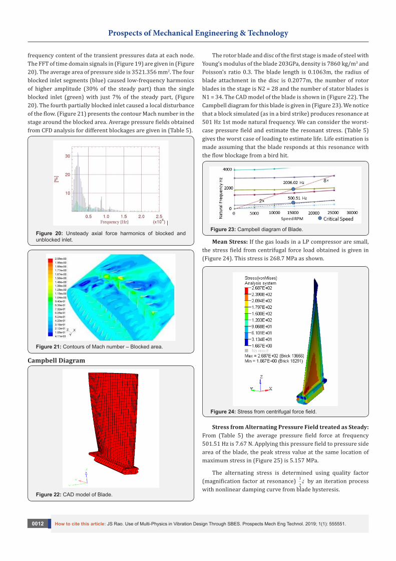
frequency content of the transient pressures data at each node. The FFT of time domain signals in (Figure 19) are given in (Figure 20). The average area of pressure side is 3521.356 mm2. The four blocked inlet segments (blue) caused low-frequency harmonics of higher amplitude (30% of the steady part) than the single blocked inlet (green) with just 7% of the steady part, (Figure 20). The fourth partially blocked inlet caused a local disturbance of the flow. (Figure 21) presents the contour Mach number in the stage around the blocked area. Average pressure fields obtained from CFD analysis for different blockages are given in (Table 5).

Figure 20: Unsteady axial force harmonics of blocked and unblocked inlet.

Figure 21: Contours of Mach number – Blocked area.

Campbell Diagram

Figure 22: CAD model of Blade.

The rotor blade and disc of the first stage is made of steel with Young’s modulus of the blade 203GPa, density is 7860 kg/m3 and Poisson’s ratio 0.3. The blade length is 0.1063m, the radius of blade attachment in the disc is 0.2077m, the number of rotor blades in the stage is N2 = 28 and the number of stator blades is N1 = 34. The CAD model of the blade is shown in (Figure 22). The Campbell diagram for this blade is given in (Figure 23). We notice that a block simulated (as in a bird strike) produces resonance at 501 Hz 1st mode natural frequency. We can consider the worst-case pressure field and estimate the resonant stress. (Table 5) gives the worst case of loading to estimate life. Life estimation is made assuming that the blade responds at this resonance with the flow blockage from a bird hit.

Figure 23: Campbell diagram of Blade.

Mean Stress: If the gas loads in a LP compressor are small, the stress field from centrifugal force load obtained is given in (Figure 24). This stress is 268.7 MPa as shown.

Figure 24: Stress from centrifugal force field.

Stress from Alternating Pressure Field treated as Steady: From (Table 5) the average pressure field force at frequency 501.51 Hz is 7.67 N. Applying this pressure field to pressure side area of the blade, the peak stress value at the same location of maximum stress in (Figure 25) is 5.157 MPa.

The alternating stress is determined using quality factor (magnification factor at resonance) 1

2ξ by an iteration process

with nonlinear damping curve from blade hysteresis.



Figure 25: Stress from alternating pressure treated as steady.

Figure 26: Orthonormal mode of the blade.

Hysteresis damping: Orthonormal mode of the blade at operating speed 15000 rpm is given in (Figure 26). The strain value at the reference element chosen 13555 is 4.173×10-04. Lazan material properties used are:

Damping coefficient J = 16 and

Exponent n = 2.3

Endurance limit eσ = 300 MPa The code Turbo Manager is used to obtain the damping

coefficient for the orthonormal mode, see (Table 6). To update the damping factor as a function of the state of the stress, the

strain values are modified as before in equations (2) to (5) by using a multiplying factor F and obtaining the damping ratios. The nonlinear damping as a function of the strain amplitude at reference point of the blade at 15000rpm in the I mode as obtained in Turbo Manager is given in (Figure 27).

Table 6: Damping calculations for orthonormal condition.

Mode I natural frequency = 3174.29rad/sec

Reference strain at element id 13555 e = 4.173×10-4

Total strain energy W0 = 27.63 N mm

Total damping energy D0 = 1.039 N mm

Loss factor h = 0.005

Equivalent viscous damping Ce = 19.0 N-s/mm

Damping ratio x = 0.0029

Damping ratio at resonance: The state of stress of the blade at resonance is not known apriori; this value depends on damping. An iteration process is adopted by assuming a damping value to begin with and determining the first approximation of resonant stress by using the stress value obtained by treating the alternating force as steady force and multiplying with the quality factor. The strain at the reference element is then determined and the revised damping value is determined from (Figure 27a). With this iterated damping we go back to determine the stress etc. until convergence occurs. This iteration process is shown in Figure 27b.

Figure 27a: Nonlinear damping in I mode at 15000 rpm as a function of strain at the reference point.

Figure 27b: Damping Iterations.



Alternating Stress: With the damping ratio from (Figure 27) taken as 0.005, the alternating stress is 5.157

515.72 0.005

=×

MPa Stress Intensity Factor Range: (Figure 28) shows the stress

raiser location of the blade.

Figure 28: Peak Stress Location and Stress Raiser.

Figure 29: Semi elliptic notch.

A semi elliptic notch model is adopted for the stress raiser location as given in (Figure 29).

The conversion for stress into stress intensity factor is given by ( )1.12 ,2

aK a k fT b

σ π λ δ∆ = ∆

(7)

where 2f and k are given in (Figure 30).

The critical crack length for unstable fracture conditions is defined by

Figure 30: Values of f2 and K.



( )

2

1 1

1.12 ,max 2

K cacr ak f

bπ

σ λ δ

=

(8)

Paris law and crack propagation: Paris law for crack propagation employed is

( )da mC K

dN= ∆ (9)

Initial crack length is taken as af∆ = 0.015mm

Notch radius ρ = 2.64 mm measured from model as shown in (Figure 28). In the notch geometry considered a/b is taken as 0.5, then from (Figure 30) k = 1.35 and f2 = 0.5.

Fracture toughness KIc is taken as 0.580MPam

Paris constant C = 0.0001356

Paris exponent m = 2.25

Incremental crack length = 100microns

For the alternating stress amplitude 515.7 MPa, the critical length calculated in Turbo Manager is 0.005m. For the crack to reach unstable conditions, the number of cycles elapsed is 3683.

The crack growth calculation is done with constant amplitude loading with stress ratio R = 0 as a function of number of elapsed cycles is given in (Figure 31).

Figure 31: Crack length vs. number of cycles.

(Figure 32) gives the striation spacing as a function of number of cycles elapsed. The striation spacing increases slowly first and then rapidly as number of cycles of alternating load

elapse. In (Figure 33) the striation spacing as a function of crack length is shown. The striation spacing increases almost linearly with elapsed number of cycles.

Figure 32: dadN as a function of number of cycles elapsed.



Figure 33: dadN vs. crack length.

The estimated crack propagation life at 15000RPM for 2× harmonic = 3683 cycles. One may then assume that the blade life in the present case of severe blockage is 3683

7 sec501.51

=

Bird ingestion that may cause aircraft engine fan blades or the first stage compressor blades to fail can be simulated by transient flow with the inlet passages blocked using a CFD code. Depending on bird hit with a single bird or from multiple birds in a flock encountered by the aircraft engine, different blockages are simulated by placing obstructions in the inlet flow with one or several struts. The transient pressure field obtained from a CFD code is used to identify the frequency components from an FFT that can cause resonance. A nonlinear damping model is developed using Lazan’s hysteresis law; the equivalent viscous damping model is determined as a function of reference strain amplitude in the given mode of vibration at the rotational speed. An iterative process is developed with the nonlinear damping model and the resonant stress and location is determined using SBES and Platform approach. The Fracture Mechanics approach is then used to estimate the crack propagation life of the blade.

Fluid Structure Interaction - Wing FlutterAerospace Engineering is a field with continued advent of

new technologies. In almost all sub-branches of Aeronautics, an excellent technological progress has been observed over the last two decades; Stability being more of significance in design of any aircraft. Multi-disciplinary optimization is being preferred over optimization for individual disciplines. Understanding of inter-disciplinary concepts such as the Fluid structure interaction is necessary for optimization of the design for better performance at minimum cost. In the Fluid structure interaction (FSI) problems, solid structures interact with an internal or external fluid flow in direct contact with them. FSI problems play significant roles in many engineering and scientific fields. Due to their strong nonlinearity and multidisciplinary nature, a

comprehensive study of such problems still remains a challenge. When a fluid interacts with a solid structure, the flow exerts a pressure on the solid surface which may cause deformation in the structure. As a result, the deformed structure changes the flow field. The altered flowing fluid exerts another form of pressure on the structure. The repetition of the process occurs continuously. This is termed as Fluid-Structure Interaction (FSI). The study of the effect of aerodynamic forces on elastic bodies is termed as Aero-elasticity.

It all began with galloping of transmission wires in the northern cold climate and then with Tacoma Narrows bridge collapse, see Rao (2011) [1]. Fortunately, today we have high speed computation available to us with a Platform approach that can couple Fluid Structure Interaction; realizing the importance and the application need, there are few commercial codes to link the fluid structure interaction, e.g., Ansys.

Flutter is most commonly seen on wings and the control surfaces of an aircraft structure. It is because of the load acting on these are the highest when an aircraft is in flight. The inertia and flexibility of the structure plays a very significant role in the aero-elastic dynamic stability of the aircraft. Self-excited and unstable oscillations due to unsteady aerodynamic forces from the air flow normally take place when a structural system which is under flow conditions beyond some threshold or critical value of the flow parameter like the dynamic pressure. Flutter can be basically a phenomenon of unstable oscillations in a flexible structure.

The usage of CFD algorithms in order to simulate and predict the aerodynamic load on the structure has been made possible by the increase in computation speed. For CFD, a Naiver-Stokes or Euler flow solver coupled with a modal structural and FEM solver can simulate, solve and give accurate predictions of aero-



elastic response of the structure. The prediction of the aero-elastic response may require a time span in the order of days because computationally intense nature of CFD.

The 2D Flutter analysis of NACA 641 A212 done previously with a two-way coupled FSI model is illustrated in (Figure 34)

with the structural and fluid domains, modal analysis results and pressure distribution over the wing surface. The vertical displacement obtained as a function of time for three velocities 100, 175 and 300 m/s loading conditions is given in (Figure 35). The flutter case can be seen here.

Figure 34: Aero elastic analysis of a NACA 641 A212 air foil.

Figure 35: Vertical Displacement vs. Time Graph of the Air foil subjected to loading conditions.

3D Flutter Analysis: A wing derived by adopting topological considerations with SIMP (Solid Isotropic material with Penalization) is used here, see Rao et al. [7]. A typical aircraft wing consists of the following components - Spars, Ribs, Stringers, Skin, Flaps and Ailerons. Spars are the structural elements that ultimately bear the load carried by the wing. Most wings have two spars and some even have up to five. After

optimization, the wing design comprised of Truss pattern for the ribs, two spars, leading edge Stringers removed, Box section for front spar and Channel section for the rear spar, L-shaped cross section for stringers close to trailing edge. The wing designed thus is shown in (Figure 36-39). The dimensions in (Figure 38) are 1. 2.68m, 2. 1.39m, 3. 4.74m, 4. 8.76m and 5. 13.5m.



Figure 36: Topology optimized wing showing the skin.

Figure 37: Topology optimized wing showing the spar and ribs.

Figure 38: Topology optimised wing with dimensions.

Figure 39: Wing modeled in ANSYS Design modeller and the structural mesh.

Figure 40: Computational Fluid Domain modelled for the analysis and the respective mesh.



(Figure 40) shows the mesh generated for the CFD analysis. The total number of nodes generated is 104742 and the number of elements is 357048. More care was taken towards refinement of the mesh to capture the flow physics exactly and to avoid negative volume error occurring due to the dynamic mesh in the analysis. The element quality parameters are: Skewness: ~0.95 and Orthogonality: ~0.02. In the analysis, Mach number is taken as 0.8 for three angles of attack, 0.05, 5 and 25 degrees [8].

The modal analysis with the Eigen values and Participation Factors is given in (Table 7). The corresponding mode shapes are given in (Figure 41). The fundamental corresponding to flapping is the first mode: 3.67 Hz. The natural time-period ~0.27sec The Participation from this (flapping) mode is ~55% of the Total Mass (9.33 ton) Considering 2 cycles, we have (0.27×2) = ~0.5 sec and thus the flutter duration considered for the analysis is 0.5s.

Table 7: Eigen Values with Participation Factors.

Mode Frequency Period Partic.factor Ratio Effective mass Cumulative Mass fraction Fatio Eff. Mass to total mass

1 3.67936 0.27179 72.005 1 5184.76 0.628378 0.355358

2 17.3833 5.75E-01 -41.965 0.582807 1761.08 0.841815 0.188635

3 20.8559 4.79E-02 -11.146 0.1548 124.243 0.856873 1.33E-02

4 41.3926 2.42E-02 25.936 0.360199 672.69 0.938401 7.21E-02

5 47.4249 2.11E-02 -10.297 0.143006 106.032 0.951252 1.14E-02

6 72.8532 1.37E-02 20.056 0.278528 402.224 1 4.31E-02

Sum 8251.03 8.84E-01

Figure 41: Modal Analysis.

The fluid structure interaction in three dimensions under transient conditions is carried out with three different cases of angle attack viz., Case 1: 0.050. Case 2: 50 and Case 3: 250. The transient responses obtained are discussed here.

a. Case 1: Angle of attack 0.050

The dynamic FSI analysis was carried out for 0.5 s at 0.050 with a time step of 0.001s. The results obtained for the fluid

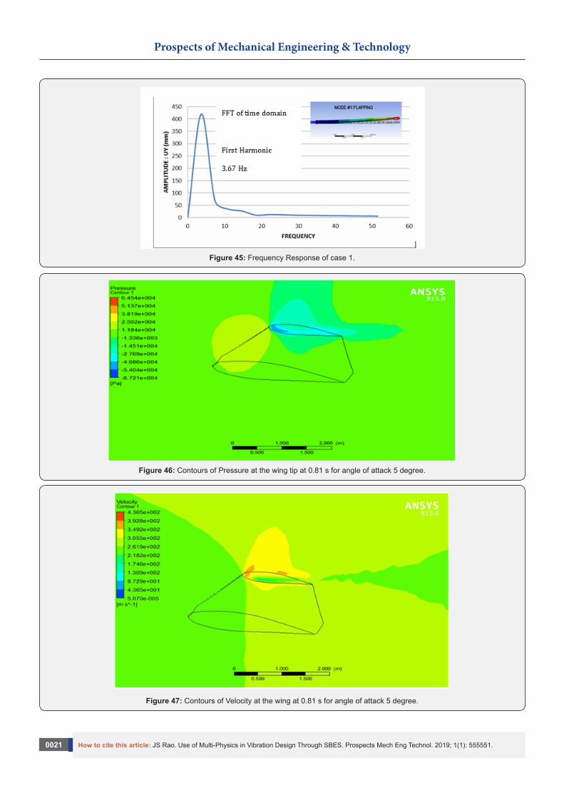
velocity at the wing tip are given in (Figure 42) at 0.5s. Similarly, the fluid pressure at the wing tip is given in (Figure 43). Transient response at the wing tip is given in (Figure 44). This clearly shows that the response is decaying without causing any flutter conditions. (Figure 45) shows the frequency response of the time domain signal. Only one peak is present corresponding to I mode 3.67Hz.



Figure 42: Contours of fluid velocity at the wing tip at 0.5 s for angle of attack 0.05 degrees.

Figure 43: Contours of fluid pressure at the wing tip at 0.5 s for angle of attack 0.05 degrees.

Figure 44: Time Response curve of the wing tip for first bending mode.



Figure 45: Frequency Response of case 1.

Figure 46: Contours of Pressure at the wing tip at 0.81 s for angle of attack 5 degree.

Figure 47: Contours of Velocity at the wing at 0.81 s for angle of attack 5 degree.



b. Case 2: Angle of Attack 50

The analysis was carried out for 0.81 s at 50 with a time step of 0.001 s. The results obtained are given in (Figure 46) for the fluid pressure at the wing tip at 0.81 s. Similarly, the fluid velocity at the wing tip is given in (Figure 47).

In (Figure 48) Pressure applied on wing exerted by the fluid is compared at the initial and final time steps as the peak

pressure rose to the nose region. (Figure 49) shows the wing displacement at the first- and last-time steps showing prevailing flutter conditions. The flow streamlines at the initial time step indicate steady conditions, whereas at the last time step, the streamlines are not steady as shown in (Figure 50). The response of the wing tip up to 0.81 s is given in (Figure 51) showing the flutter condition.

Figure 48: Comparison of Pressure applied on wing exerted by the fluid for angle of attack 5°.

Figure 49: Wing deformation at the first- and last-time steps.



Figure 50: Streamlines of velocity over the wing at the first- and last-time step at 0.81 s.

Figure 51: Time Response curve of the wing tip up to 0.81 s for angle of attack 5 degree.

Figure 52: Contours of pressure at the wing tip at 0.327 s for angle of attack 25 degree.



c. Case 3: Angle of Attack 250

By increasing the angle of attack further the flutter is expected to be severe. In this case the response increased rapidly, and the

numerical instability terminated the run at 0.327s. The dynamic (Figures 52 & 53) give the fluid pressure and velocity at the wing tip at 0.327s respectively. (Figure 54) gives the vibration amplitude at the wing tip which shows no oscillation.

Figure 53: Contours of velocity of fluid at the wing tip at 0.327 s for angle of attack 25 degree.

Figure 54: Vibration amplitude Vs. Time curve of the wing tip.

ClosureMulti-Physics developed during Science Revolution period

could not be applied till the advent of High-Performance Computing; instead the complete sciences were approximated at the beginning of last century. With the development of Digital computers during the Second World War, the sciences in original form bounced back making the engineering approach into domain approach. The advances in this century bringing SBES and HPC particularly being utilized for advanced engineering applications in aerospace industry are given to highlight in engines and structures.

References1. Rao J S (2011) History of Rotating Machinery Dynamics, Springer,

Germany.

2. Rao J S (2018) Creativity in design–Science to engineering model. Mechanism and Machine Theory 125: 52-79.

3. Rao J S (1991) Turbomachine Blade Vibration. John Wiley, USA.

4. Rao J S (2000) Turbine Blade Life Estimation. Alpha Science International Limited, UK.

5. Rao J S, Ratnakar R, Soliński M, Narayanan R, Rzadkowsky R (2012) Life Calculation of First Stage Compressor Blade of a Trainer Aircraft. ASME Turbo Expo, Copenhagen, Denmark: 11-15.

6. Rao J S (Srinivasa R Jammi), Rzadkowsky R (2014) Crack Propagation Life Calculation of an Aircraft Compressor Blade due to Bird Ingestion. Proceedings of the ASME Turbo Expo, Dusseldorf, Germany: 16-20.

7. Rao JS, Tharikaa R K, Shivakumar P (2015) Flutter of Aircraft Wing, ICVE 2015, Shanghai, China: 18-20.

8. Rao J S, Ratnakar R, Suresh S, Narayanan R, (2009) A Procedure to Predict Influence of Acceleration and Damping of Blades Passing



Through Critical Speeds on Fatigue Life. Proceedings of ASME Turbo Expo, Power for Land, Sea and Air, Orlando, Florida, USA, GT2009-5943: 8-12.

This work is licensed under CreativeCommons Attribution 4.0 License

Your next submission with Juniper Publishers will reach you the below assets

• Quality Editorial service• Swift Peer Review• Reprints availability• E-prints Service• Manuscript Podcast for convenient understanding• Global attainment for your research• Manuscript accessibility in different formats

( Pdf, E-pub, Full Text, Audio) • Unceasing customer service

Track the below URL for one-step submission https://juniperpublishers.com/online-submission.php

https://juniperpublishers.com/online-submission.php

Use of Multi-Physics in Vibration Design Through SBES

Documents

Transcript of Use of Multi-Physics in Vibration Design Through SBES