Urban Schools - National Center for Education Statistics ...nces.ed.gov/pubs/96184all.pdf · Urban...
228
NATIONAL CENTER FOR EDUCATION STATISTICS Urban Schoo ls The Challenge of Location and Poverty U.S. Department of Education Office of Educational Research and Improvement NCES 96-184
Transcript of Urban Schools - National Center for Education Statistics ...nces.ed.gov/pubs/96184all.pdf · Urban...

NATIONAL CENTER FOR EDUCATION STATISTICS
Urban SchoolsThe Challenge of Location
and Poverty
U.S. Department of EducationOffice of Educational Research and Improvement NCES 96-184

NATIONAL CENTER FOR EDUCATION STATISTICS
June 1996
Urban SchoolsThe Challenge of Locationand Poverty
Laura LippmanShelley BurnsEdith McArthurNational Center for Education Statistics
With contributions by:Robert BurtonThomas M. SmithNational Center for Education Statistics
Phil KaufmanMPR Associates, Inc.
U.S. Department of EducationOffice of Educational Research and Improvement NCES 96-184

U.S. Department of EducationRichard W. RileySecretary
Office of Educational Research and ImprovementSharon P. RobinsonAssistant Secretary
National Center for Education StatisticsJeanne E. GriffithActing Commissioner
Data Development and Longitudinal Studies GroupJohn H. RalphActing Associate Commissioner
National Center for Education Statistics
“The purpose of the Center shall be to collect, andanalyze, and disseminate statistics and other datarelated to education in the United States and inother nations.”—Section 406(b) of the GeneralEducation Provisions Act, as amended (20 U.S.C. 1221e-1).
June 1996

Page
Foreword . . . . . . . . . . . . . . . . . . . . . . . . . . . . . . . . . . . . . . . . . . . . . . . . . . . . . . . . . . . . . . . . . . . . . . . iiiAcknowledgments . . . . . . . . . . . . . . . . . . . . . . . . . . . . . . . . . . . . . . . . . . . . . . . . . . . . . . . . . . . . . . . . . ivExecutive Summary . . . . . . . . . . . . . . . . . . . . . . . . . . . . . . . . . . . . . . . . . . . . . . . . . . . . . . . . . . . . . . . . .vList of Figures . . . . . . . . . . . . . . . . . . . . . . . . . . . . . . . . . . . . . . . . . . . . . . . . . . . . . . . . . . . . . . . . . . . xviList of Charts and Tables . . . . . . . . . . . . . . . . . . . . . . . . . . . . . . . . . . . . . . . . . . . . . . . . . . . . . . . . . . xxvii
1. INTRODUCTION . . . . . . . . . . . . . . . . . . . . . . . . . . . . . . . . . . . . . . . . . . . . . . . . . . . . . . . . . . . . . 1Previous Research on School Location and Poverty Concentration . . . . . . . . . . . . . . . . . . . . . . . . . . . . 2
Student Level . . . . . . . . . . . . . . . . . . . . . . . . . . . . . . . . . . . . . . . . . . . . . . . . . . . . . . . . . . . . . . . . . 2School Level . . . . . . . . . . . . . . . . . . . . . . . . . . . . . . . . . . . . . . . . . . . . . . . . . . . . . . . . . . . . . . . . . 2Neighborhood Level . . . . . . . . . . . . . . . . . . . . . . . . . . . . . . . . . . . . . . . . . . . . . . . . . . . . . . . . . . . . 3
The Setting: Urban Schools and Communities . . . . . . . . . . . . . . . . . . . . . . . . . . . . . . . . . . . . . . . . . . 4Urban Schools . . . . . . . . . . . . . . . . . . . . . . . . . . . . . . . . . . . . . . . . . . . . . . . . . . . . . . . . . . . . . . . . 4School Poverty Concentration . . . . . . . . . . . . . . . . . . . . . . . . . . . . . . . . . . . . . . . . . . . . . . . . . . . . . 5Student Minority Status . . . . . . . . . . . . . . . . . . . . . . . . . . . . . . . . . . . . . . . . . . . . . . . . . . . . . . . . . 8Community Risk Factors . . . . . . . . . . . . . . . . . . . . . . . . . . . . . . . . . . . . . . . . . . . . . . . . . . . . . . . 11
Approach . . . . . . . . . . . . . . . . . . . . . . . . . . . . . . . . . . . . . . . . . . . . . . . . . . . . . . . . . . . . . . . . . . . . 13Sources . . . . . . . . . . . . . . . . . . . . . . . . . . . . . . . . . . . . . . . . . . . . . . . . . . . . . . . . . . . . . . . . . . . . . . 16Definitions of Urbanicity and Poverty Concentration . . . . . . . . . . . . . . . . . . . . . . . . . . . . . . . . . . . . . 17
2. EDUCATION OUTCOMES . . . . . . . . . . . . . . . . . . . . . . . . . . . . . . . . . . . . . . . . . . . . . . . . . . . . . 19Summary of This Chapter’s Findings . . . . . . . . . . . . . . . . . . . . . . . . . . . . . . . . . . . . . . . . . . . . . . . 20
Student Achievement . . . . . . . . . . . . . . . . . . . . . . . . . . . . . . . . . . . . . . . . . . . . . . . . . . . . . . . . . . . . 24Findings . . . . . . . . . . . . . . . . . . . . . . . . . . . . . . . . . . . . . . . . . . . . . . . . . . . . . . . . . . . . . . . . . . . 24
Academic Achievement of 8th Graders . . . . . . . . . . . . . . . . . . . . . . . . . . . . . . . . . . . . . . . . . . . . 26Academic Achievement of 10th Graders . . . . . . . . . . . . . . . . . . . . . . . . . . . . . . . . . . . . . . . . . . . 28Did 10th-Grade Achievement Change Between 1980 and 1990? . . . . . . . . . . . . . . . . . . . . . . . . . . 30
Educational Attainment . . . . . . . . . . . . . . . . . . . . . . . . . . . . . . . . . . . . . . . . . . . . . . . . . . . . . . . . . . 31Findings . . . . . . . . . . . . . . . . . . . . . . . . . . . . . . . . . . . . . . . . . . . . . . . . . . . . . . . . . . . . . . . . . . . 31
High School Completion . . . . . . . . . . . . . . . . . . . . . . . . . . . . . . . . . . . . . . . . . . . . . . . . . . . . . . 32Postsecondary Degree Attainment . . . . . . . . . . . . . . . . . . . . . . . . . . . . . . . . . . . . . . . . . . . . . . . . 34
Economic Outcomes . . . . . . . . . . . . . . . . . . . . . . . . . . . . . . . . . . . . . . . . . . . . . . . . . . . . . . . . . . . . 36Findings . . . . . . . . . . . . . . . . . . . . . . . . . . . . . . . . . . . . . . . . . . . . . . . . . . . . . . . . . . . . . . . . . . . 36
Early Productive Activities . . . . . . . . . . . . . . . . . . . . . . . . . . . . . . . . . . . . . . . . . . . . . . . . . . . . . 38Later Productive Activities . . . . . . . . . . . . . . . . . . . . . . . . . . . . . . . . . . . . . . . . . . . . . . . . . . . . . 40Unemployment . . . . . . . . . . . . . . . . . . . . . . . . . . . . . . . . . . . . . . . . . . . . . . . . . . . . . . . . . . . . . 42Poverty Status . . . . . . . . . . . . . . . . . . . . . . . . . . . . . . . . . . . . . . . . . . . . . . . . . . . . . . . . . . . . . . 44
Page xiii
Contents

Contents—ContinuedPage
3. STUDENT BACKGROUND CHARACTERISTICS AND AFTERSCHOOL ACTIVITIES . . . . . . . 47 Summary of This Chapter’s Findings . . . . . . . . . . . . . . . . . . . . . . . . . . . . . . . . . . . . . . . . . . . . . . . 48
Student Background Characteristics . . . . . . . . . . . . . . . . . . . . . . . . . . . . . . . . . . . . . . . . . . . . . . . . . 51Findings . . . . . . . . . . . . . . . . . . . . . . . . . . . . . . . . . . . . . . . . . . . . . . . . . . . . . . . . . . . . . . . . . . . 51
Two-Parent Families . . . . . . . . . . . . . . . . . . . . . . . . . . . . . . . . . . . . . . . . . . . . . . . . . . . . . . . . . .52Parental Employment . . . . . . . . . . . . . . . . . . . . . . . . . . . . . . . . . . . . . . . . . . . . . . . . . . . . . . . . . 54Parents’ Educational Attainment . . . . . . . . . . . . . . . . . . . . . . . . . . . . . . . . . . . . . . . . . . . . . . . . . 58School Mobility . . . . . . . . . . . . . . . . . . . . . . . . . . . . . . . . . . . . . . . . . . . . . . . . . . . . . . . . . . . . . 60Parents’ Expectations for Their Child’s Education . . . . . . . . . . . . . . . . . . . . . . . . . . . . . . . . . . . . 62Parent and Child Conversations About School . . . . . . . . . . . . . . . . . . . . . . . . . . . . . . . . . . . . . . . 64
Afterschool Activities . . . . . . . . . . . . . . . . . . . . . . . . . . . . . . . . . . . . . . . . . . . . . . . . . . . . . . . . . . . . 67Findings . . . . . . . . . . . . . . . . . . . . . . . . . . . . . . . . . . . . . . . . . . . . . . . . . . . . . . . . . . . . . . . . . . . 67
Student Participation in Extracurricular Sports . . . . . . . . . . . . . . . . . . . . . . . . . . . . . . . . . . . . . . 67School Sports Offerings . . . . . . . . . . . . . . . . . . . . . . . . . . . . . . . . . . . . . . . . . . . . . . . . . . . . . . 68Sports Participation . . . . . . . . . . . . . . . . . . . . . . . . . . . . . . . . . . . . . . . . . . . . . . . . . . . . . . . . 70
Employment of 10th-Grade Students . . . . . . . . . . . . . . . . . . . . . . . . . . . . . . . . . . . . . . . . . . . . . 72
4. SCHOOL EXPERIENCES . . . . . . . . . . . . . . . . . . . . . . . . . . . . . . . . . . . . . . . . . . . . . . . . . . . . . . . 75Summary of This Chapter’s Findings . . . . . . . . . . . . . . . . . . . . . . . . . . . . . . . . . . . . . . . . . . . . . . . 76
School Resources and Staff . . . . . . . . . . . . . . . . . . . . . . . . . . . . . . . . . . . . . . . . . . . . . . . . . . . . . . . . 81Findings . . . . . . . . . . . . . . . . . . . . . . . . . . . . . . . . . . . . . . . . . . . . . . . . . . . . . . . . . . . . . . . . . . . 81
Availability of Resources . . . . . . . . . . . . . . . . . . . . . . . . . . . . . . . . . . . . . . . . . . . . . . . . . . . . . . . 82Teacher Salaries . . . . . . . . . . . . . . . . . . . . . . . . . . . . . . . . . . . . . . . . . . . . . . . . . . . . . . . . . . . . . 84Teacher Experience . . . . . . . . . . . . . . . . . . . . . . . . . . . . . . . . . . . . . . . . . . . . . . . . . . . . . . . . . . 86Difficulty Hiring Teachers . . . . . . . . . . . . . . . . . . . . . . . . . . . . . . . . . . . . . . . . . . . . . . . . . . . . . 88Percent Minority Teachers . . . . . . . . . . . . . . . . . . . . . . . . . . . . . . . . . . . . . . . . . . . . . . . . . . . . . 90Teacher Gender . . . . . . . . . . . . . . . . . . . . . . . . . . . . . . . . . . . . . . . . . . . . . . . . . . . . . . . . . . . . . 92Teacher Influence Over Curriculum . . . . . . . . . . . . . . . . . . . . . . . . . . . . . . . . . . . . . . . . . . . . . . 94Teacher Absenteeism . . . . . . . . . . . . . . . . . . . . . . . . . . . . . . . . . . . . . . . . . . . . . . . . . . . . . . . . . 96
School Programs and Coursetaking . . . . . . . . . . . . . . . . . . . . . . . . . . . . . . . . . . . . . . . . . . . . . . . . . . 98Findings . . . . . . . . . . . . . . . . . . . . . . . . . . . . . . . . . . . . . . . . . . . . . . . . . . . . . . . . . . . . . . . . . . . 98
Preschool Attendance . . . . . . . . . . . . . . . . . . . . . . . . . . . . . . . . . . . . . . . . . . . . . . . . . . . . . . . . 100Gifted and Talented Programs . . . . . . . . . . . . . . . . . . . . . . . . . . . . . . . . . . . . . . . . . . . . . . . . . . 102Vocational Coursetaking . . . . . . . . . . . . . . . . . . . . . . . . . . . . . . . . . . . . . . . . . . . . . . . . . . . . . . 104Mathematics Coursetaking . . . . . . . . . . . . . . . . . . . . . . . . . . . . . . . . . . . . . . . . . . . . . . . . . . . . 106
Student Behavior . . . . . . . . . . . . . . . . . . . . . . . . . . . . . . . . . . . . . . . . . . . . . . . . . . . . . . . . . . . . . . 108Findings . . . . . . . . . . . . . . . . . . . . . . . . . . . . . . . . . . . . . . . . . . . . . . . . . . . . . . . . . . . . . . . . . . 108
Hours of Television Watched on Weekdays . . . . . . . . . . . . . . . . . . . . . . . . . . . . . . . . . . . . . . . . 110Hours Spent on Homework . . . . . . . . . . . . . . . . . . . . . . . . . . . . . . . . . . . . . . . . . . . . . . . . . . . 112Student Absenteeism . . . . . . . . . . . . . . . . . . . . . . . . . . . . . . . . . . . . . . . . . . . . . . . . . . . . . . . . 114Time Spent Maintaining Classroom Discipline . . . . . . . . . . . . . . . . . . . . . . . . . . . . . . . . . . . . . 116School Safety . . . . . . . . . . . . . . . . . . . . . . . . . . . . . . . . . . . . . . . . . . . . . . . . . . . . . . . . . . . . . . 118
Page xiv

Contents—ContinuedPage
Student Possession of Weapons . . . . . . . . . . . . . . . . . . . . . . . . . . . . . . . . . . . . . . . . . . . . . . . . . 120Student Alcohol Use . . . . . . . . . . . . . . . . . . . . . . . . . . . . . . . . . . . . . . . . . . . . . . . . . . . . . . . . 122Student Pregnancy . . . . . . . . . . . . . . . . . . . . . . . . . . . . . . . . . . . . . . . . . . . . . . . . . . . . . . . . . .124
APPENDICESA Estimates and Standard Error Tables . . . . . . . . . . . . . . . . . . . . . . . . . . . . . . . . . . . . . . . . . . . . . A-1B Methodology of Analysis . . . . . . . . . . . . . . . . . . . . . . . . . . . . . . . . . . . . . . . . . . . . . . . . . . . . . B-1C Technical Notes . . . . . . . . . . . . . . . . . . . . . . . . . . . . . . . . . . . . . . . . . . . . . . . . . . . . . . . . . . . . C-1D Data Sources and Definitions . . . . . . . . . . . . . . . . . . . . . . . . . . . . . . . . . . . . . . . . . . . . . . . . . . D-1E Bibliography . . . . . . . . . . . . . . . . . . . . . . . . . . . . . . . . . . . . . . . . . . . . . . . . . . . . . . . . . . . . . . E-1
Page xv
In the past, analytic reports prepared by the NationalCenter for Education Statistics (NCES) have used thedata available from one of our survey programs toaddress a variety of issues. In this report, we haveattempted to do something different. We have chosensome specific policy-relevant questions and have triedto answer them using data from several of our surveysas well as other federal surveys.
The questions we chose illuminate the condition ofeducation in urban schools compared to schools inother locations. Much attention has been givenrecently to America’s urban schools, which areperceived to be in a state of some deterioration.Critics like Jonathan Kozol (Savage Inequalities) havevividly pointed out the problems with run-down facilities,unmotivated teachers, crime, and low expectations ininner city schools based on firsthand observations.Many believe that urban youth are more at risk todaythan youth living elsewhere. Information on theseyouths is important to the Department of Educationbecause our mission is to ensure equal access to a highquality education for all.
We thought we could add to the existing informationby exploring differences between students from urban
schools and students in other locations on a broadspectrum of student and school characteristics. Inparticular, we explored how the concentration of studentpoverty in schools is related to these differences. To dothis, we used sophisticated analytical methodologies,but we hope the results are still easy to understand.Our goal was to provide useful information for peopleinterested in the relationship of poverty and urbanicityto student outcomes and background characteristics,as well as school and teacher characteristics.
To help us in planning for future analyses, we wouldwelcome your reaction to this report. Did it answersome important questions about urban schools foryou? Were the results easy to understand? Did it providea “big picture” of urban schools? Did it suggest otherissues or topics that could be addressed in a similarmanner? The answers to these questions will help usto gauge the success of our effort to produce a newtype of report, analyzing a particular topic with rele-vant data from various sources. We are continuallystriving to improve our reports to make them morerelevant, accessible, and thought provoking.
Jeanne E. GriffithActing Commissioner
Page iii
Foreword

The authors wish to acknowledge the contributionsmade by the many people involved with this projectat every stage of its development.
The analysis of data from many surveys could nothave been accomplished without the help and expertiseof NCES survey directors and staff and our colleaguesat MPR Associates and Pinkerton ComputerConsultants. We wish to thank Jeff Owens, JerryWest, Sharon Bobbitt, and Alex Sedlecek of NCES fortheir willingness to take the time to share their exper-tise with us, and John Tuma and Phil Kaufman ofMPR Associates for their analytical work. BruceDaniel of Pinkerton Computer Consultants efficient-ly and cheerfully provided endless tabulations of datafrom multiple surveys.
Mary Frase, John Ralph, and Bob Burton offeredhelpful suggestions to the write-up and formatting ofthe indicators, which markedly improved the presen-tation. Jenny Manlove helped write a section of thereport in chapter 1 on community level backgroundcharacteristics.
The report was reviewed by very thoughtful and gen-erous people both within and outside of NCES, whoimproved the report immeasurably. Our NCESreviewers included Mary Frase, Bob Burton, John
Ralph, Jeanne Griffith, Jerry West, Paula Knepper,Sharon Bobbitt, and Kerry Gruber. Our externalreviewers included Michael Casserly, Gary Natriello,Floraline Stevens, and Donald Hernandez. Their con-tributions were innumerable, but any remaining flawsare ours alone.
The project generated many activities at MPRAssociates that were orchestrated by the conscientiouswork of Fena Neustaedter, Patty Holmes, and SusieKagehiro. Andrea Livingston expertly edited thereport, and Leslie Retallick’s design for the layout andgraphics greatly enhanced the report. Elliott Medrichprovided helpful editorial suggestions and took on thetask of orchestrating the final editing and layout.Dawn Nelson at NCES handled the administrativeaspects of contracting with MPR Associates and pro-vided last-minute assistance with writing. SuellenMauchamer orchestrated the production of the report.
The authors particularly wish to thank John Ralph forhis inspiration, enthusiasm and support throughoutthe project, and Jeanne Griffith for her insights, support,and patience. This project took on many challenges,and its success was directly due to the willingness ofEmerson Elliott, while Commissioner, and JeanneGriffith, currently Acting Commissioner, to allow theauthors to pursue the paths where the analysis led.
Page iv
Acknowledgments

Many Americans believe that urban schools are failingto educate the students they serve. Even among peoplewho think that schools are doing a good job overallare those who believe that in certain schools, conditionsare abysmal. Their perception, fed by numerousreports and observations, is that urban studentsachieve less in school, attain less education, andencounter less success in the labor market later in life.
Researchers and educators often link this perceivedperformance of urban youth to home and school envi-ronments that do not foster educational and economicsuccess. Moreover, urban educators report the grow-ing challenges of educating urban youth who areincreasingly presenting problems such as poverty, lim-ited English proficiency, family instability, and poorhealth. Finally, testimony and reports on the condi-tion of urban schools feed the perception that urbanstudents flounder in decaying, violent environmentswith poor resources, teachers, and curricula, and withlimited opportunities.
This report addresses these widespread beliefs aboutthe performance of urban students, and their familyand school environments. Using data from severalnational surveys, it compares urban students andschools with their suburban and rural counterparts ona broad range of factors, including student populationand background characteristics, afterschool activities,school experiences, and student outcomes.
A specific focus of this report is how poverty relates tothe characteristics of the students and schools studied.Since, on average, urban public schools are more like-ly to serve low income students, it is possible that anydifferences between urban and non-urban schools andstudents are due to this higher concentration of lowincome students. In this study, the methodology usedto explore differences between urban, suburban, andrural students and schools incorporates a control forthe concentration of poverty in the school. Thus, thisstudy allows comparisons to be made between urbanand other schools and students, after factoring out
one major characteristic of urban schools that is oftenrelated to differences between schools—the higherconcentration of low income students.
In addition, this report focuses on those urban schoolsthat serve the highest concentrations of low incomestudents, in light of national concern over theseschools. Previous research has suggested that studentsfrom schools with high concentrations of low incomestudents and students from urban schools would beexpected to have less successful educational outcomes,less supportive home environments, and less positiveschool experiences than students from other schools.In fact, this study finds large differences betweenurban and non-urban schools and between highpoverty and low poverty schools on most of the indi-cators of student background, school experiences, andstudent outcomes studied.
Students attending schools with both an urban loca-tion and a high poverty concentration were expected,therefore, to have particularly unfavorable circum-stances. This report documents how urban highpoverty schools and their students compare with theircounterparts in other locations across many areas ofconcern, according to national surveys. Furthermore,the analysis specifically examines whether theseschools and students compare less favorably than pre-dicted, when considering together the effects ofpoverty concentration and an urban location. If thedifferences between urban high poverty schools andothers are no greater than predicted, it indicates thatthe circumstances in these schools are related in pre-dicted ways to the effects of poverty concentrationand an urban location added together. However, if thedifferences are greater than predicted, it indicates thatthe effects of poverty concentration and locationinteract, and that the level for that particular measureexceeds the level that was predicted from these twoeffects alone. When this occurs, urban high povertyschools and their students are said to compare partic-ularly unfavorably (or favorably, as the case may be) toother schools on that measure.
Page v
Urban Schools
Executive Summary

Student Characteristics
This study describes students who attended publicschools primarily in the 1980s and examines theiroutcomes through 1990. Although the number ofstudents in urban schools remained stable at about 11million between 1980 and 1990, the proportion ofthose students who were living in poverty or who haddifficulty speaking English increased over the decade.The proportion of students in urban schools whobelonged to an Hispanic or “other” minority group(which includes Asians and Pacific Islanders)increased over the decade, while the proportion whowere white declined and the proportion who wereblack stayed about the same. The increasing propor-tion of children with non-English backgrounds inurban locations has led to a greater proportion of chil-dren with difficulty speaking English in those locations.
Urban children were more than twice as likely to beliving in poverty than those in suburban locations (30percent compared with 13 percent in 1990), while 22percent of rural children were poor in 1990 (figure A). Likewise, urban students were more likely than sub-urban or rural students to receive free or reduced pricelunch (38 percent compared with 16 and 28 percent,
respectively). It follows then, that urban students weremore likely to be attending schools with high concen-trations of low income students. Forty percent ofurban students attended these high poverty schools(defined as schools with more than 40 percent of stu-dents receiving free or reduced price lunch), whereas10 percent of suburban students and 25 percent ofrural students did so (figure B). Previous research sug-gests that a high concentration of low incomestudents in a school is related to less desirable studentperformance.
Aside from the greater likelihood of being poor andhaving difficulty speaking English, urban studentswere more likely than suburban students to beexposed to risks that research has associated with lessdesirable outcomes. Urban students were more likelyto be exposed to safety and health risks that placetheir health and well-being in jeopardy, and were lesslikely to have access to regular medical care. Theywere also more likely to engage in risk-taking behav-ior, such as teenage pregnancy, that can makedesirable outcomes more difficult to reach.
Page vi
SOURCE: U.S. Bureau of the Census, Current PopulationReports, Series P-60, Nos. 181 and 133.
Figure APoverty rates for children under 18, by urbanicity:
1980 and 1990
20
Percent
Total
5
10
15
25
30
17.919.9
26.2
30.0
11.212.5
19.4
22.2
Urban Suburban Rural
1980 1990
35
0
Percent
0
50
17.2
12.1
35.5
11.7
25.8
38.7
22.0
31.8
Total Urban Suburban Rural
25.0 26.0
40.1
15.6
10.2
32.3 31.5
24.5
40
30
20
10
6Ð20 21Ð40 Over 40
Percent receiving free and reduced-price lunch
0Ð5
Figure BPercentage distribution of students, by school
poverty concentration within urbanicity categories:1987–88
SOURCE: U.S. Department of Education, National Center forEducation Statistics, Schools and Staffing Survey, 1987–88.
Seepage 5
Seepage 7

Student Background Characteristics and AfterschoolActivities
Urban students were equally or more likely than otherstudents to have families with certain characteristicsthat have been found to support desirable educationoutcomes, including high parental educational attain-ment, high expectations for their children'seducation, and frequent communication aboutschool. However, there were some important excep-tions. They were less likely to have the familystructure, economic security, and stability that aremost associated with desirable educational outcomes.
This section and those that follow use the analysismethodology described above to compare urban stu-dents with students in other locations whileaccounting for differences in school poverty concen-tration, and to compare students in urban highpoverty schools with those in other high povertyschools. When compared to their suburban and ruralcounterparts, students in urban and urban high povertyschools were
• at least as likely to have a parent who completedcollege (figure C);
• at least as likely to have parents with high expec-tations for their education; and
• as likely to have parents who talked with themabout school.
However, they were
• less likely to live in two-parent families (figure D);
• more likely to have changed schools frequently; and
• less likely than some but not all other groups tohave at least one parent in a two-parent familyworking.
When examining their afterschool activities, studentsin urban schools, overall, were just as likely to beoffered school sports activities and to work afterschool as students in schools elsewhere, but were lesslikely to participate in school-sponsored sports activi-ties, even after accounting for poverty concentration.The afterschool experiences of students in urban highpoverty schools were similar to those of students inhigh poverty schools in other locations.
Page vii
School poverty concentration(percent)
0 to 5 6 to 20 21 to 40 Over 40
Percent
Suburban
Urban
Rural
0
10
20
30
40
50
Figure CPercentage of 8th-grade students with a parent in the
household who had completed 4 years of college,by urbanicity and school poverty concentration:
1988
SOURCE: U.S. Department of Education, National Center forEducation Statistics, National Education Longitudinal Study of1988, Base Year Survey.
SOURCE: U.S. Department of Education, National Center forEducation Statistics, National Education Longitudinal Study of1988, Base Year Survey.
Figure DPercentage of 8th-grade students living in a two-parentfamily, by urbanicity and school poverty concentration:
1988Percent
School poverty concentration(percent)
0 to 5 6 to 20 21 to 40 Over 40
SuburbanUrban
Rural
0
50
60
70
80
90
Seepage 59
Seepage 53
Page viii
In all of the student background and afterschool char-acteristics studied, students in urban high povertyschools compared in predicted ways to those in otherschools. The differences between these students andstudents in other schools were related to the effects ofpoverty concentration and an urban location added together.
School Experiences
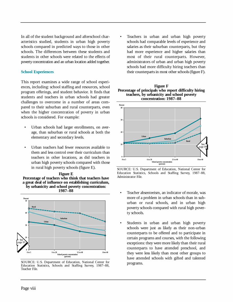
This report examines a wide range of school experi-ences, including: school staffing and resources, schoolprogram offerings, and student behavior. It finds thatstudents and teachers in urban schools had greaterchallenges to overcome in a number of areas com-pared to their suburban and rural counterparts, evenwhen the higher concentration of poverty in urbanschools is considered. For example:
• Urban schools had larger enrollments, on aver-age, than suburban or rural schools at both theelementary and secondary levels.
• Urban teachers had fewer resources available tothem and less control over their curriculum thanteachers in other locations, as did teachers inurban high poverty schools compared with thosein rural high poverty schools (figure E).
• Teachers in urban and urban high povertyschools had comparable levels of experience andsalaries as their suburban counterparts, but theyhad more experience and higher salaries thanmost of their rural counterparts. However,administrators of urban and urban high povertyschools had more difficulty hiring teachers thantheir counterparts in most other schools (figure F).
• Teacher absenteeism, an indicator of morale, wasmore of a problem in urban schools than in sub-urban or rural schools, and in urban highpoverty schools compared with rural high pover-ty schools.
• Students in urban and urban high povertyschools were just as likely as their non-urbancounterparts to be offered and to participate incertain programs and courses, with the followingexceptions: they were more likely than their ruralcounterparts to have attended preschool, andthey were less likely than most other groups tohave attended schools with gifted and talentedprograms.
Figure EPercentage of teachers who think that teachers havea great deal of influence on establishing curriculum,
by urbanicity and school poverty concentration:1987–88
Percent
0 to 5 6 to 20 21 to 40 Over 40
Suburban
Urban
Rural
0
20
30
40
50
School poverty concentration(percent)
SOURCE: U.S. Department of Education, National Center forEducation Statistics, Schools and Staffing Survey, 1987–88,Teacher File.
SOURCE: U.S. Department of Education, National Center forEducation Statistics, Schools and Staffing Survey, 1987–88,Administrator File.
Figure FPercentage of principals who report difficulty hiring
teachers, by urbanicity and school povertyconcentration: 1987–88
Percent
SuburbanUrban
Rural
0
10
20
40
School poverty concentration(percent)
30
0 to 5 6 to 20 21 to 40 Over 40
Seepage 95
Seepage 89

Page ix
• Student behavior problems were more commonin urban schools than in other schools, particu-larly in the areas of student absenteeism,classroom discipline (figure G), weapons posses-sion, and student pregnancy. However, the use ofalcohol was less of a problem in urban schoolsthan in rural schools.
• Students in high poverty schools regardless oflocation were less likely to feel safe in school, orto spend much time on homework than those inlow poverty schools. However, students in urbanhigh poverty schools were much more likely towatch television excessively (figure H) and torequire more discipline by teachers in class com-pared with their counterparts in other locations;they were also more likely to be absent and pos-sess weapons than those in rural high povertyschools.
Among the school experiences studied, urban highpoverty schools and their students exceeded the levelspredicted when considering the effects of urbanicityand poverty concentration in three areas: students
were more likely to watch television excessively, lesslikely to have access to gifted and talented programs,and were more likely to have minority teachers (con-sidered by many to be a favorable circumstance). Thelevels of these indicators were unusual when com-pared with non-urban schools, and were not explainedsolely by the effects of poverty concentration and loca-tion added together.
Urban high poverty schools often compared unfavor-ably to rural high poverty schools on measures ofschool experiences, but were often similar to suburbanhigh poverty schools on these measures. Furtheranalysis suggested that high poverty concentration inrural schools was not as strongly related to students’school experiences as it was in urban or suburbanschools.
Student Outcomes
Many of the student background characteristics andschool experiences of urban students outlined abovewould suggest that students in urban and particularlyurban high poverty schools had greater challenges toovercome than did suburban or rural students in
SOURCE: U.S. Department of Education, National Center forEducation Statistics, National Education Longitudinal Study of1988, Base Year Teacher File.
Figure GPercentage of teachers of 8th-grade students who
spend at least 1 hour per week maintainingclassroom order and discipline, by urbanicity and
school poverty concentration: 1988
Percent
0 to 5 6 to 20 21 to 40 Over 40
Suburban
Urban
Rural
0
10
20
30
40
School poverty concentration(percent)
SOURCE: U.S. Department of Education, National Center forEducation Statistics, National Education Longitudinal Study of1988, First Follow-up Student File.
Figure HPercentage of 10th-grade students who watch 3 or
more hours of television on weekdays, by urbanicity and school poverty concentration: 1990
Percent
0 to 5 6 to 20 21 to 40 Over 40
Suburban
Urban
Rural
0
20
30
40
50
School poverty concentration(percent)
Seepage 117
Seepage 111

Page x
achieving academically, attaining education, andencountering success in the labor market. This studyfinds important differences in the achievement,attainment, and economic outcomes of urban stu-dents compared with those in other locations. Thesedifferences were more pronounced at younger agesand many diminish with age. However, for a minori-ty of students who attended urban schools, thelikelihood of long-term poverty and unemploymentwas much greater than for those who attended schoolin other locations.
When urban students were compared with suburbanand rural students, while accounting for the higherconcentration of poverty in urban schools, and whenstudents in urban high poverty schools were com-pared with those in other high poverty schools:
• 8th graders in urban and urban high povertyschools scored lower on achievement tests, buttheir 10th-grade counterparts scored about thesame as those in other locations.
• Students in urban and urban high poverty schoolswere less likely to complete high school on time(figure I), but they completed postsecondarydegrees at the same rate as others.
• Young adults who had attended urban schools hadlower rates of participation in full-time work orschool 4 years after most of them would have lefthigh school, but had similar participation rates 7 to15 years after high school; those from urban highpoverty schools had levels of activity that were sim-ilar to those from other high poverty schools.
• Young adults who had attended urban and urbanhigh poverty schools had much higher povertyand unemployment rates later in life than thosewho had attended other schools (figures J and K).
Although students in urban high poverty schoolscompared less favorably than students in high povertyschools located elsewhere on many measures, it isimportant to keep their absolute levels of performancein mind. Despite the challenges that students fromurban high poverty schools face, the great majority ofthese students graduated from high school on time(66 percent), and during their young adult years, weremore likely than not to be employed or to be in schoolfull time (73 percent), and were living above thepoverty line (74 percent).
The levels of the outcomes measured for studentsfrom urban high poverty schools would have been
Figure IPercentage graduating on time among the
sophomore class of 1980, by urbanicity and percentdisadvantaged in school
Percent
0 to 5 6 to 20 21 to 40 Over 40
Suburban
Urban
Rural
0
65
75
85
90
95
Percent disadvantaged in school
80
70
SOURCE: U.S. Department of Education, National Center forEducation Statistics, High School and Beyond Study, ThirdFollow-up Survey, 1986.
SOURCE: U.S. Department of Labor, National Longitudinal Surveyof Youth, 1990.
Figure JPercentage of young adults living in poverty, by high
school urbanicity and percent disadvantaged inhigh school: 1990
Percent
0 to 5 6 to 20 21 to 40 Over 40
Suburban
Urban
Rural
0
5
20
25
30
Percent disadvantaged in school
10
15
Seepage 33
Seepage 45

Page xi
predicted from the effects of poverty concentrationand an urban location added together. Given the largeoverall variation on these measures by urbanicity andpoverty concentration, the outcomes for these stu-dents were not unusual.
Discussion
Looking across all of the measures of student back-ground, school experiences, and student outcomesstudied, some general findings emerge:
• Urban students and schools compared less favor-ably to their non-urban counterparts on manymeasures even after accounting for the higherconcentration of low income students in urbanschools.
• Urban high poverty schools and their studentsperformed similarly or more favorably thanother high poverty schools and students on halfof the measures studied. On these measures,large differences were found by school povertyconcentration, so that high poverty concentra-
tion seemed to present equally challenging cir-cumstances in all locations.
• On the other half of the measures studied, urbanhigh poverty schools and their students com-pared unfavorably to other high poverty schools.These measures tended to show consistent dif-ferences by location across the levels of povertyconcentration.
• When considering the large overall variations bylocation and poverty concentration, urban highpoverty schools and their students, with fewexceptions, were no different than the effects oflocation and poverty concentration addedtogether would have predicted.
Previous research has suggested that students fromschools with high concentrations of low income stu-dents, and students from urban schools would haveless supportive family backgrounds, less favorableschool experiences, and less successful educationaloutcomes than students from other schools. Thisstudy provides evidence that students in urbanschools are more likely than those in other locationsto have characteristics such as poverty, difficultyspeaking English, and numerous health and safetyrisks that present greater challenges to them and theireducators. This study also provides evidence thatimportant differences do exist between the studentbackground characteristics, school experiences, andoutcomes of urban and other students, and that thesedifferences represent more than that which can beattributed to differences in the school concentrationof low income students. When these differencesremain after accounting for poverty concentration, itis possible that the above-cited differences betweenurban and non-urban student characteristics, or otherdifferences between urban, suburban, and rural loca-tions come into play.
However, in every domain of students’ lives studied—student background characteristics, school experiences,and student outcomes—there were instances whereurban students and schools were similar to their non-
SOURCE: U.S. Department of Labor, National Longitudinal Surveyof Youth, 1990.
Figure KPercentage of young adults unemployed, by high
school urbanicity and percent disadvantagedin high school: 1990
Percent
0 to 5 6 to 20 21 to 40 Over 40
Suburban
UrbanRural
0
2
8
10
12
Percent disadvantaged in school
4
6
Seepage 43

urban counterparts after accounting for poverty concen-tration, suggesting that some of the often-cited bleakperceptions of urban schools and students may be over-stated. Given the greater challenges that urban studentsand schools face, the fact that they were similar to theirnon-urban counterparts on these measures suggests thatthey may not only be meeting the challenges, but per-forming above expectations in these areas.
Moreover, this report provides evidence that chal-lenges the perception that urban schools with thehighest poverty concentrations are always much worseoff than other schools. The report documents largevariations in schools and students in all of the impor-tant areas considered when assessing schoolperformance—student background, school experi-ences, and student outcomes. Within this overallvariation, differences between urban high povertyschools and other high poverty schools did not usuallyexceed differences between urban and other schools atother levels of poverty concentration. On half of themeasures, urban high poverty schools did compareunfavorably to high poverty schools in other locations;however, in an equal number of cases, urban highpoverty schools were similar or even compared favorably.
The findings from this study suggest certain areaswhere the differences between the student background,school experiences, and outcomes of students in urbanand other schools—particularly in urban high povertyschools compared with other high poverty schools—are
most pronounced. These areas could benefit from fur-ther research:
Student Background
• Single-parent families
• School mobility
School Experiences
• Difficulty hiring teachers
• Teacher control over curriculum
• Weekday television watching
• Student absenteeism
• Classroom discipline
• Weapons possession
• Student pregnancy
Student Outcomes
• High school completion
• Poverty and unemployment of young adults
Page xii

Page xvi
Figure Page
Executive Summary
Figure A Poverty rates for children under 18, by urbanicity: 1980 and 1990 . . . . . . . . . . . . . . . . . . . . vi
Figure B Percentage distribution of students, by school poverty concentrationwithin urbanicity categories: 1987–88 . . . . . . . . . . . . . . . . . . . . . . . . . . . . . . . . . . . . . . . . . vi
Figure C Percentage of 8th-grade students with a parent in the householdwho had completed 4 years of college, by urbanicityand school poverty concentration: 1988 . . . . . . . . . . . . . . . . . . . . . . . . . . . . . . . . . . . . . . . vii
Figure D Percentage of 8th-grade students living in a two-parent family, by urbanicity and school poverty concentration: 1988 . . . . . . . . . . . . . . . . . . . . . . . . . . . . . . . . . . . . . . . . . . vii
Figure E Percentage of teachers who think that teachers have a great deal of influence on establishingcurriculum in their school, by urbanicity and school poverty concentration:1987–88 . . . . . . . . . . . . . . . . . . . . . . . . . . . . . . . . . . . . . . . . . . . . . . . . . . . . . . . . . . . . . viii
Figure F Percentage of principals who report difficulty hiring teachers, by urbanicity andschool poverty concentration: 1987–88 . . . . . . . . . . . . . . . . . . . . . . . . . . . . . . . . . . . . . . . viii
Figure G Percentage of teachers of 8th-grade students who spend at least 1 hour per weekmaintaining classroom order and discipline, by urbanicity andschool poverty concentration: 1988 . . . . . . . . . . . . . . . . . . . . . . . . . . . . . . . . . . . . . . . . . . . ix
Figure H Percentage of 10th-grade students who watch 3 or more hours of television on weekdays,by urbanicity and school poverty concentration: 1990 . . . . . . . . . . . . . . . . . . . . . . . . . . . . . ix
Figure I Percentage graduating on time among the sophomore class of 1980,by urbanicity and percent disadvantaged in school . . . . . . . . . . . . . . . . . . . . . . . . . . . . . . . . x
Figure J Percentage of young adults living in poverty, by high school urbanicity andpercent disadvantaged in high school: 1990 . . . . . . . . . . . . . . . . . . . . . . . . . . . . . . . . . . . . . x
Figure K Percentage of young adults unemployed, by high school urbanicity andpercent disadvantaged in high school: 1990 . . . . . . . . . . . . . . . . . . . . . . . . . . . . . . . . . . . . . xi
List of Figures

Figure Page
Chapter 1 Introduction
Figure 1.1 Number of students enrolled in public schools, by urbanicity:1980 and 1990 . . . . . . . . . . . . . . . . . . . . . . . . . . . . . . . . . . . . . . . . . . . . . . . . . . . . . . . . . . 4
Figure 1.2 Percentage distribution of students enrolled in public schools, by urbanicity:1980 and 1990 . . . . . . . . . . . . . . . . . . . . . . . . . . . . . . . . . . . . . . . . . . . . . . . . . . . . . . . . . . 5
Figure 1.3 Poverty rates for children under age 18, by urbanicity:1980 and 1990 . . . . . . . . . . . . . . . . . . . . . . . . . . . . . . . . . . . . . . . . . . . . . . . . . . . . . . . . . . 5
Figure 1.4 Percentage of 8th graders whose family was in the lowest socioeconomic quartile,by urbanicity: 1988 . . . . . . . . . . . . . . . . . . . . . . . . . . . . . . . . . . . . . . . . . . . . . . . . . . . . . . 6
Figure 1.5 Percentage of students in poverty-related programs, by urbanicity:1987–88 . . . . . . . . . . . . . . . . . . . . . . . . . . . . . . . . . . . . . . . . . . . . . . . . . . . . . . . . . . . . . . 6
Figure 1.6 Percentage distribution of students, by school poverty concentrationwithin urbanicity categories: 1987–88 . . . . . . . . . . . . . . . . . . . . . . . . . . . . . . . . . . . . . . . . . 7
Figure 1.7 Percentage distribution of students by school poverty concentration deciles,by urbanicity: 1987–88 . . . . . . . . . . . . . . . . . . . . . . . . . . . . . . . . . . . . . . . . . . . . . . . . . . . . 8
Figure 1.8 Percentage of students with difficulty speaking English, by urbanicity:1979 and 1989 . . . . . . . . . . . . . . . . . . . . . . . . . . . . . . . . . . . . . . . . . . . . . . . . . . . . . . . . . . 8
Figure 1.9 Trends in the racial-ethnic distribution of urban students:1980 and 1990 . . . . . . . . . . . . . . . . . . . . . . . . . . . . . . . . . . . . . . . . . . . . . . . . . . . . . . . . . . 9
Figure 1.10 Racial-ethnic distribution of students, by urbanicity: 1987–88 . . . . . . . . . . . . . . . . . . . . . . . 9
Figure 1.11 Racial-ethnic distribution of students in schools, by urbanicity andschool poverty concentration: 1987–88 . . . . . . . . . . . . . . . . . . . . . . . . . . . . . . . . . . . . . . . 10
Figure 1.12 Victimization rates for persons ages 12 and over, by type of crimeand urbanicity: 1990 . . . . . . . . . . . . . . . . . . . . . . . . . . . . . . . . . . . . . . . . . . . . . . . . . . . . . 11
Figure 1.13 Infant mortality rates, by urbanicity: 1990 . . . . . . . . . . . . . . . . . . . . . . . . . . . . . . . . . . . . . 12
Figure 1.14 Percentage of children 17 years of age and under whose regular sourceof health care is a clinic, health center, or hospital emergency room,by urbanicity: 1988 . . . . . . . . . . . . . . . . . . . . . . . . . . . . . . . . . . . . . . . . . . . . . . . . . . . . . . 12
Page xvii
Page xviii
Figure Page
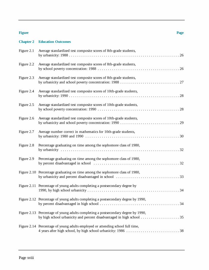
Chapter 2 Education Outcomes
Figure 2.1 Average standardized test composite scores of 8th-grade students,by urbanicity: 1988 . . . . . . . . . . . . . . . . . . . . . . . . . . . . . . . . . . . . . . . . . . . . . . . . . . . . . . 26
Figure 2.2 Average standardized test composite scores of 8th-grade students,by school poverty concentration: 1988 . . . . . . . . . . . . . . . . . . . . . . . . . . . . . . . . . . . . . . . . 26
Figure 2.3 Average standardized test composite scores of 8th-grade students,by urbanicity and school poverty concentration: 1988 . . . . . . . . . . . . . . . . . . . . . . . . . . . . . 27
Figure 2.4 Average standardized test composite scores of 10th-grade students,by urbanicity: 1990 . . . . . . . . . . . . . . . . . . . . . . . . . . . . . . . . . . . . . . . . . . . . . . . . . . . . . . 28
Figure 2.5 Average standardized test composite scores of 10th-grade students,by school poverty concentration: 1990 . . . . . . . . . . . . . . . . . . . . . . . . . . . . . . . . . . . . . . . . 28
Figure 2.6 Average standardized test composite scores of 10th-grade students,by urbanicity and school poverty concentration: 1990 . . . . . . . . . . . . . . . . . . . . . . . . . . . . . 29
Figure 2.7 Average number correct in mathematics for 10th-grade students,by urbanicity: 1980 and 1990 . . . . . . . . . . . . . . . . . . . . . . . . . . . . . . . . . . . . . . . . . . . . . . 30
Figure 2.8 Percentage graduating on time among the sophomore class of 1980,by urbanicity . . . . . . . . . . . . . . . . . . . . . . . . . . . . . . . . . . . . . . . . . . . . . . . . . . . . . . . . . . 32
Figure 2.9 Percentage graduating on time among the sophomore class of 1980,by percent disadvantaged in school . . . . . . . . . . . . . . . . . . . . . . . . . . . . . . . . . . . . . . . . . . 32
Figure 2.10 Percentage graduating on time among the sophomore class of 1980,by urbanicity and percent disadvantaged in school . . . . . . . . . . . . . . . . . . . . . . . . . . . . . . . 33
Figure 2.11 Percentage of young adults completing a postsecondary degree by 1990, by high school urbanicity . . . . . . . . . . . . . . . . . . . . . . . . . . . . . . . . . . . . . . . . . . . . . 34
Figure 2.12 Percentage of young adults completing a postsecondary degree by 1990,by percent disadvantaged in high school . . . . . . . . . . . . . . . . . . . . . . . . . . . . . . . . . . . . . . . 34
Figure 2.13 Percentage of young adults completing a postsecondary degree by 1990,by high school urbanicity and percent disadvantaged in high school . . . . . . . . . . . . . . . . . . . 35
Figure 2.14 Percentage of young adults employed or attending school full time,4 years after high school, by high school urbanicity: 1986 . . . . . . . . . . . . . . . . . . . . . . . . . . 38

Figure Page
Figure 2.15 Percentage of young adults employed or attending school full time,4 years after high school, by percent disadvantagedin high school: 1986 . . . . . . . . . . . . . . . . . . . . . . . . . . . . . . . . . . . . . . . . . . . . . . . . . . . . . 38
Figure 2.16 Percentage of young adults employed or attending school full time,4 years after high school, by high school urbanicity andpercent disadvantaged in high school: 1986 . . . . . . . . . . . . . . . . . . . . . . . . . . . . . . . . . . . . 39
Figure 2.17 Percentage of young adults employed or attending school full time,by high school urbanicity: 1990 . . . . . . . . . . . . . . . . . . . . . . . . . . . . . . . . . . . . . . . . . . . . . 40
Figure 2.18 Percentage of young adults employed or attending school full time,by percent disadvantaged in high school: 1990 . . . . . . . . . . . . . . . . . . . . . . . . . . . . . . . . . . 40
Figure 2.19 Percentage of young adults employed or attending school full time,by high school urbanicity and percent disadvantagedin high school: 1990 . . . . . . . . . . . . . . . . . . . . . . . . . . . . . . . . . . . . . . . . . . . . . . . . . . . . . 41
Figure 2.20 Percentage of young adults unemployed, by high school urbanicity:1990 . . . . . . . . . . . . . . . . . . . . . . . . . . . . . . . . . . . . . . . . . . . . . . . . . . . . . . . . . . . . . . . . 42
Figure 2.21 Percentage of young adults unemployed, by percent disadvantagedin high school: 1990 . . . . . . . . . . . . . . . . . . . . . . . . . . . . . . . . . . . . . . . . . . . . . . . . . . . . . 42
Figure 2.22 Percentage of young adults unemployed, by high school urbanicity andpercent disadvantaged in high school: 1990 . . . . . . . . . . . . . . . . . . . . . . . . . . . . . . . . . . . . 43
Figure 2.23 Percentage of young adults living in poverty, by high school urbanicity:1990 . . . . . . . . . . . . . . . . . . . . . . . . . . . . . . . . . . . . . . . . . . . . . . . . . . . . . . . . . . . . . . . . 44
Figure 2.24 Percentage of young adults living in poverty, by percent disadvantagedin high school: 1990 . . . . . . . . . . . . . . . . . . . . . . . . . . . . . . . . . . . . . . . . . . . . . . . . . . . . . 44
Figure 2.25 Percentage of young adults living in poverty, by high school urbanicity andpercent disadvantaged in high school: 1990 . . . . . . . . . . . . . . . . . . . . . . . . . . . . . . . . . . . . 45
Chapter 3 Student Background Characteristics and Afterschool Activities
Figure 3.1 Percentage of 8th-grade students living in a two-parent family,by urbanicity: 1988 . . . . . . . . . . . . . . . . . . . . . . . . . . . . . . . . . . . . . . . . . . . . . . . . . . . . . . 52
Figure 3.2 Percentage of 8th-grade students living in a two-parent family,by school poverty concentration: 1988 . . . . . . . . . . . . . . . . . . . . . . . . . . . . . . . . . . . . . . . . 52
Page xix
Page xx
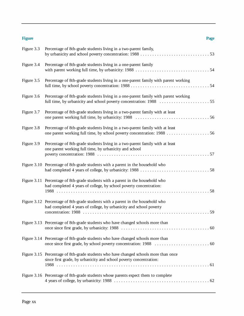
Figure Page
Figure 3.3 Percentage of 8th-grade students living in a two-parent family,by urbanicity and school poverty concentration: 1988 . . . . . . . . . . . . . . . . . . . . . . . . . . . . . 53
Figure 3.4 Percentage of 8th-grade students living in a one-parent familywith parent working full time, by urbanicity: 1988 . . . . . . . . . . . . . . . . . . . . . . . . . . . . . . . 54
Figure 3.5 Percentage of 8th-grade students living in a one-parent family with parent workingfull time, by school poverty concentration: 1988 . . . . . . . . . . . . . . . . . . . . . . . . . . . . . . . . . 54
Figure 3.6 Percentage of 8th-grade students living in a one-parent family with parent workingfull time, by urbanicity and school poverty concentration: 1988 . . . . . . . . . . . . . . . . . . . . . 55
Figure 3.7 Percentage of 8th-grade students living in a two-parent family with at leastone parent working full time, by urbanicity: 1988 . . . . . . . . . . . . . . . . . . . . . . . . . . . . . . . 56
Figure 3.8 Percentage of 8th-grade students living in a two-parent family with at leastone parent working full time, by school poverty concentration: 1988 . . . . . . . . . . . . . . . . . . 56
Figure 3.9 Percentage of 8th-grade students living in a two-parent family with at leastone parent working full time, by urbanicity and school poverty concentration: 1988 . . . . . . . . . . . . . . . . . . . . . . . . . . . . . . . . . . . . . . . . . . . . . . . 57
Figure 3.10 Percentage of 8th-grade students with a parent in the household whohad completed 4 years of college, by urbanicity: 1988 . . . . . . . . . . . . . . . . . . . . . . . . . . . . . 58
Figure 3.11 Percentage of 8th-grade students with a parent in the household whohad completed 4 years of college, by school poverty concentration:1988 . . . . . . . . . . . . . . . . . . . . . . . . . . . . . . . . . . . . . . . . . . . . . . . . . . . . . . . . . . . . . . . . 58
Figure 3.12 Percentage of 8th-grade students with a parent in the household whohad completed 4 years of college, by urbanicity and school poverty concentration: 1988 . . . . . . . . . . . . . . . . . . . . . . . . . . . . . . . . . . . . . . . . . . . . . . . . . . . . . 59
Figure 3.13 Percentage of 8th-grade students who have changed schools more thanonce since first grade, by urbanicity: 1988 . . . . . . . . . . . . . . . . . . . . . . . . . . . . . . . . . . . . . 60
Figure 3.14 Percentage of 8th-grade students who have changed schools more thanonce since first grade, by school poverty concentration: 1988 . . . . . . . . . . . . . . . . . . . . . . . 60
Figure 3.15 Percentage of 8th-grade students who have changed schools more than oncesince first grade, by urbanicity and school poverty concentration:1988 . . . . . . . . . . . . . . . . . . . . . . . . . . . . . . . . . . . . . . . . . . . . . . . . . . . . . . . . . . . . . . . . 61
Figure 3.16 Percentage of 8th-grade students whose parents expect them to complete4 years of college, by urbanicity: 1988 . . . . . . . . . . . . . . . . . . . . . . . . . . . . . . . . . . . . . . . . 62

Figure Page
Figure 3.17 Percentage of 8th-grade students whose parents expect them to complete4 years of college, by school poverty concentration: 1988 . . . . . . . . . . . . . . . . . . . . . . . . . . 62
Figure 3.18 Percentage of 8th-grade students whose parents expect them to complete4 years of college, by urbanicity and school poverty concentration:1988 . . . . . . . . . . . . . . . . . . . . . . . . . . . . . . . . . . . . . . . . . . . . . . . . . . . . . . . . . . . . . . . . 63
Figure 3.19 Percentage of 8th-grade students whose parents rarely talk to themabout school, by urbanicity: 1988 . . . . . . . . . . . . . . . . . . . . . . . . . . . . . . . . . . . . . . . . . . . 64
Figure 3.20 Percentage of 8th-grade students whose parents rarely talk to them about school,by school poverty concentration: 1988 . . . . . . . . . . . . . . . . . . . . . . . . . . . . . . . . . . . . . . . . 64
Figure 3.21 Percentage of 8th-grade students whose parents rarely talk to them about school,by urbanicity and school poverty concentration: 1988 . . . . . . . . . . . . . . . . . . . . . . . . . . . . . 65
Figure 3.22 Average number of sports-related activities offered by the schools attendedby 10th-grade students, by urbanicity: 1990 . . . . . . . . . . . . . . . . . . . . . . . . . . . . . . . . . . . . 68
Figure 3.23 Average number of sports-related activities offered by the schools attendedby 10th-grade students, by school poverty concentration:1990 . . . . . . . . . . . . . . . . . . . . . . . . . . . . . . . . . . . . . . . . . . . . . . . . . . . . . . . . . . . . . . . . 68
Figure 3.24 Average number of sports-related activities offered by the schools attendedby 10th-grade students, by urbanicity and schoolpoverty concentration: 1990 . . . . . . . . . . . . . . . . . . . . . . . . . . . . . . . . . . . . . . . . . . . . . . . 69
Figure 3.25 Percentage of 10th-grade students who participated in sports-related activities,by urbanicity: 1990 . . . . . . . . . . . . . . . . . . . . . . . . . . . . . . . . . . . . . . . . . . . . . . . . . . . . . . 70
Figure 3.26 Percentage of 10th-grade students who participated in sports-related activities,by school poverty concentration: 1990 . . . . . . . . . . . . . . . . . . . . . . . . . . . . . . . . . . . . . . . . 70
Figure 3.27 Percentage of 10th-grade students who participated in sports-related activities,by urbanicity and school poverty concentration: 1990 . . . . . . . . . . . . . . . . . . . . . . . . . . . . . 71
Figure 3.28 Percentage of 10th-grade students who worked 11 or more hours per week,by urbanicity: 1990 . . . . . . . . . . . . . . . . . . . . . . . . . . . . . . . . . . . . . . . . . . . . . . . . . . . . . . 72
Figure 3.29 Percentage of 10th-grade students who worked 11 or more hours per week,by school poverty concentration: 1990 . . . . . . . . . . . . . . . . . . . . . . . . . . . . . . . . . . . . . . . . 72
Figure 3.30 Percentage of 10th-grade students who worked 11 or more hours per week,by urbanicity and school poverty concentration: 1990 . . . . . . . . . . . . . . . . . . . . . . . . . . . . . 73
Page xxi

Page xxii
Figure Page
Chapter 4 School Experiences
Figure 4.1 Percentage of teachers who agreed that necessary materials are availablein their schools, by urbanicity: 1987–88 . . . . . . . . . . . . . . . . . . . . . . . . . . . . . . . . . . . . . . . 82
Figure 4.2 Percentage of teachers who agreed that necessary materials are availablein their schools, by school poverty concentration: 1987–88 . . . . . . . . . . . . . . . . . . . . . . . . . 82
Figure 4.3 Percentage of teachers who agreed that necessary materials are availablein their schools, by urbanicity and school poverty concentration:1987–88 . . . . . . . . . . . . . . . . . . . . . . . . . . . . . . . . . . . . . . . . . . . . . . . . . . . . . . . . . . . . . 83
Figure 4.4 Average academic base teacher salary, by urbanicity: 1987–88 . . . . . . . . . . . . . . . . . . . . . . . 84
Figure 4.5 Average academic base teacher salary, by school poverty concentration:1987–88 . . . . . . . . . . . . . . . . . . . . . . . . . . . . . . . . . . . . . . . . . . . . . . . . . . . . . . . . . . . . . 84
Figure 4.6 Average academic base teacher salary, by urbanicity and school povertyconcentration: 1987–88 . . . . . . . . . . . . . . . . . . . . . . . . . . . . . . . . . . . . . . . . . . . . . . . . . . 85
Figure 4.7 Percentage of teachers with 3 years or less teaching experience,by urbanicity: 1987–88 . . . . . . . . . . . . . . . . . . . . . . . . . . . . . . . . . . . . . . . . . . . . . . . . . . . 86
Figure 4.8 Percentage of teachers with 3 years or less teaching experience,by school poverty concentration: 1987–88 . . . . . . . . . . . . . . . . . . . . . . . . . . . . . . . . . . . . . 86
Figure 4.9 Percentage of teachers with 3 years or less teaching experience,by urbanicity and school poverty concentration: 1987–88 . . . . . . . . . . . . . . . . . . . . . . . . . . 87
Figure 4.10 Percentage of principals who report difficulty hiring teachers, by urbanicity:1987–88 . . . . . . . . . . . . . . . . . . . . . . . . . . . . . . . . . . . . . . . . . . . . . . . . . . . . . . . . . . . . . 88
Figure 4.11 Percentage of principals who report difficulty hiring teachers,by school poverty concentration: 1987–88 . . . . . . . . . . . . . . . . . . . . . . . . . . . . . . . . . . . . . 88
Figure 4.12 Percentage of principals who report difficulty hiring teachers,by urbanicity and school poverty concentration: 1987–88 . . . . . . . . . . . . . . . . . . . . . . . . . . 89
Figure 4.13 Percentage of teachers who are minority, by urbanicity: 1987–88 . . . . . . . . . . . . . . . . . . . . . 90
Figure 4.14 Percentage of teachers who are minority, by school poverty concentration:1987–88 . . . . . . . . . . . . . . . . . . . . . . . . . . . . . . . . . . . . . . . . . . . . . . . . . . . . . . . . . . . . . 90
Figure 4.15 Percentage of teachers who are minority, by urbanicity and school povertyconcentration: 1987–88 . . . . . . . . . . . . . . . . . . . . . . . . . . . . . . . . . . . . . . . . . . . . . . . . . . 91

Figure Page
Figure 4.16 Percentage of secondary school teachers who are male, by urbanicity:1987–88 . . . . . . . . . . . . . . . . . . . . . . . . . . . . . . . . . . . . . . . . . . . . . . . . . . . . . . . . . . . . . 92
Figure 4.17 Percentage of secondary school teachers who are male, by school povertyconcentration: 1987–88 . . . . . . . . . . . . . . . . . . . . . . . . . . . . . . . . . . . . . . . . . . . . . . . . . . 92
Figure 4.18 Percentage of secondary school teachers who are male, by urbanicityand school poverty concentration: 1987–88 . . . . . . . . . . . . . . . . . . . . . . . . . . . . . . . . . . . . 93
Figure 4.19 Percentage of teachers who think that teachers have a great deal of influenceon establishing curriculum, by urbanicity: 1987–88 . . . . . . . . . . . . . . . . . . . . . . . . . . . . . . 94
Figure 4.20 Percentage of teachers who think that teachers have a great deal of influenceon establishing curriculum, by school poverty concentration:1987–88 . . . . . . . . . . . . . . . . . . . . . . . . . . . . . . . . . . . . . . . . . . . . . . . . . . . . . . . . . . . . . 94
Figure 4.21 Percentage of teachers who think that teachers have a great deal of influenceon establishing curriculum, by urbanicity and schoolpoverty concentration: 1987–88 . . . . . . . . . . . . . . . . . . . . . . . . . . . . . . . . . . . . . . . . . . . . 95
Figure 4.22 Percentage of teachers who consider teacher absenteeism a problemin their school, by urbanicity: 1987–88 . . . . . . . . . . . . . . . . . . . . . . . . . . . . . . . . . . . . . . . 96
Figure 4.23 Percentage of teachers who consider teacher absenteeism a problemin their school, by school poverty concentration: 1987–88 . . . . . . . . . . . . . . . . . . . . . . . . . 96
Figure 4.24 Percentage of teachers who consider teacher absenteeism a problemin their school, by urbanicity and school povertyconcentration: 1987–88 . . . . . . . . . . . . . . . . . . . . . . . . . . . . . . . . . . . . . . . . . . . . . . . . . . 97
Figure 4.25 Percentage of 8th-grade students who attended preschool,by urbanicity: 1988 . . . . . . . . . . . . . . . . . . . . . . . . . . . . . . . . . . . . . . . . . . . . . . . . . . . . . 100
Figure 4.26 Percentage of 8th-grade students who attended preschool,by school poverty concentration: 1988 . . . . . . . . . . . . . . . . . . . . . . . . . . . . . . . . . . . . . . . 100
Figure 4.27 Percentage of 8th-grade students who attended preschool,by urbanicity and school poverty concentration: 1988 . . . . . . . . . . . . . . . . . . . . . . . . . . . . 101
Figure 4.28 Percentage of elementary schools that offer gifted and talentedprograms, by urbanicity: 1987–88 . . . . . . . . . . . . . . . . . . . . . . . . . . . . . . . . . . . . . . . . . . 102
Figure 4.29 Percentage of elementary schools that offer gifted and talentedprograms, by school poverty concentration: 1987–88 . . . . . . . . . . . . . . . . . . . . . . . . . . . . 102
Page xxiii
Page xxiv
Figure Page
Figure 4.30 Percentage of elementary schools that offer gifted and talented programs, by urbanicity and school poverty concentration: 1987–88 . . . . . . . . . . . . . . . . . . . . . . . . . 103
Figure 4.31 Percentage of graduating high school seniors who took 6 or more creditsin vocational education, by urbanicity: 1990 . . . . . . . . . . . . . . . . . . . . . . . . . . . . . . . . . . . 104
Figure 4.32 Percentage of graduating high school seniors who took 6 or more creditsin vocational education, by school poverty concentration: 1990 . . . . . . . . . . . . . . . . . . . . . 104
Figure 4.33 Percentage of graduating high school seniors who took geometry, by urbanicity:1990 . . . . . . . . . . . . . . . . . . . . . . . . . . . . . . . . . . . . . . . . . . . . . . . . . . . . . . . . . . . . . . . 106
Figure 4.34 Percentage of graduating high school seniors who took geometry, by school poverty concentration: 1990 . . . . . . . . . . . . . . . . . . . . . . . . . . . . . . . . . . . . . . . . . . . . . . . . . . . . 106
Figure 4.35 Percentage of 10th-grade students who watch 3 or more hours of televisionon weekdays, by urbanicity: 1990 . . . . . . . . . . . . . . . . . . . . . . . . . . . . . . . . . . . . . . . . . . 110
Figure 4.36 Percentage of 10th-grade students who watch 3 or more hours of televisionon weekdays, by school poverty concentration: 1990 . . . . . . . . . . . . . . . . . . . . . . . . . . . . . 110
Figure 4.37 Percentage of 10th-grade students who watch 3 or more hours of televisionon weekdays, by urbanicity and school poverty concentration:1990 . . . . . . . . . . . . . . . . . . . . . . . . . . . . . . . . . . . . . . . . . . . . . . . . . . . . . . . . . . . . . . . 111
Figure 4.38 Average number of hours 10th-grade students spend on homework per week,by urbanicity: 1990 . . . . . . . . . . . . . . . . . . . . . . . . . . . . . . . . . . . . . . . . . . . . . . . . . . . . . 112
Figure 4.39 Average number of hours 10th-grade students spend on homework per week,by school poverty concentration: 1990 . . . . . . . . . . . . . . . . . . . . . . . . . . . . . . . . . . . . . . . 112
Figure 4.40 Average number of hours 10th-grade students spend on homework per week,by urbanicity and school poverty concentration: 1990 . . . . . . . . . . . . . . . . . . . . . . . . . . . . 113
Figure 4.41 Percentage of secondary teachers who believe that student absenteeismis a problem in their school, by urbanicity: 1987–88 . . . . . . . . . . . . . . . . . . . . . . . . . . . . . 114
Figure 4.42 Percentage of secondary teachers who believe that student absenteeismis a problem in their school, by school poverty concentration:1987–88 . . . . . . . . . . . . . . . . . . . . . . . . . . . . . . . . . . . . . . . . . . . . . . . . . . . . . . . . . . . . 114
Figure 4.43 Percentage of secondary teachers who believe that student absenteeismis a problem in their school, by urbanicity and school poverty concentration: 1987–88 . . . . . . . . . . . . . . . . . . . . . . . . . . . . . . . . . . . . . . . . . . . . . . . . . 115

Figure Page
Figure 4.44 Percentage of teachers of 8th-grade students who spend at least 1 hour per week maintaining classroom order and discipline, by urbanicity:1988 . . . . . . . . . . . . . . . . . . . . . . . . . . . . . . . . . . . . . . . . . . . . . . . . . . . . . . . . . . . . . . . 116
Figure 4.45 Percentage of teachers of 8th-grade students who spend at least 1 hourper week maintaining classroom order and discipline, by school poverty concentration: 1988 . . . . . . . . . . . . . . . . . . . . . . . . . . . . . . . . . . . . . . . . . . . . . . . . . . . . 116
Figure 4.46 Percentage of teachers of 8th-grade students who spend at least 1 hourper week maintaining classroom order and discipline, by urbanicity and school poverty concentration: 1988 . . . . . . . . . . . . . . . . . . . . . . . . . . . . . . . . . . . . . . . . . 117
Figure 4.47 Percentage of 10th-grade students who do not feel safe at school,by urbanicity: 1990 . . . . . . . . . . . . . . . . . . . . . . . . . . . . . . . . . . . . . . . . . . . . . . . . . . . . . 118
Figure 4.48 Percentage of 10th-grade students who do not feel safe at school, by schoolpoverty concentration: 1990 . . . . . . . . . . . . . . . . . . . . . . . . . . . . . . . . . . . . . . . . . . . . . . 118
Figure 4.49 Percentage of 10th-grade students who do not feel safe at school,by urbanicity and school poverty concentration: 1990 . . . . . . . . . . . . . . . . . . . . . . . . . . . . 119
Figure 4.50 Percentage of secondary teachers who believe that student weapons possessionis a problem in their school, by urbanicity: 1987–88 . . . . . . . . . . . . . . . . . . . . . . . . . . . . . 120
Figure 4.51 Percentage of secondary teachers who believe that student weapons possessionis a problem in their school, by school poverty concentration:1987–88 . . . . . . . . . . . . . . . . . . . . . . . . . . . . . . . . . . . . . . . . . . . . . . . . . . . . . . . . . . . . 120
Figure 4.52 Percentage of secondary teachers who believe that student weapons possessionis a problem in their school, by urbanicity and school povertyconcentration: 1987–88 . . . . . . . . . . . . . . . . . . . . . . . . . . . . . . . . . . . . . . . . . . . . . . . . . 121
Figure 4.53 Percentage of secondary teachers who think that student alcohol useis a problem in their school, by urbanicity: 1987–88 . . . . . . . . . . . . . . . . . . . . . . . . . . . . . 122
Figure 4.54 Percentage of secondary teachers who think that student alcohol use is a problemin their school, by school poverty concentration: 1987–88 . . . . . . . . . . . . . . . . . . . . . . . . . 122
Figure 4.55 Percentage of secondary teachers who think that student alcohol useis a problem in their school, by urbanicity and school povertyconcentration: 1987–88 . . . . . . . . . . . . . . . . . . . . . . . . . . . . . . . . . . . . . . . . . . . . . . . . . 123
Figure 4.56 Percentage of secondary teachers who think that student pregnancyis a problem in their school, by urbanicity: 1987–88 . . . . . . . . . . . . . . . . . . . . . . . . . . . . . 124
Page xxv

Page xxvi
Figure Page
Figure 4.57 Percentage of secondary teachers who think that student pregnancy is a problemin their school, by school poverty concentration: 1987–88 . . . . . . . . . . . . . . . . . . . . . . . . . 124
Figure 4.58 Percentage of secondary teachers who think that student pregnancy is a problemin their school, by urbanicity and school poverty concentration:1987–88 . . . . . . . . . . . . . . . . . . . . . . . . . . . . . . . . . . . . . . . . . . . . . . . . . . . . . . . . . . . . 125

Chart Page
Chart 2.1 Summary of Results: Education Outcomes . . . . . . . . . . . . . . . . . . . . . . . . . . . . . . . . . . . . 22
Chart 3.1 Summary of Results: Student Background Characteristics andAfterschool Activities . . . . . . . . . . . . . . . . . . . . . . . . . . . . . . . . . . . . . . . . . . . . . . . . . . . . 49
Chart 4.1 Summary of Results: School Experiences . . . . . . . . . . . . . . . . . . . . . . . . . . . . . . . . . . . . . . 77
APPENDIX A
Table
Table 1.1 Data and standard errors for figures 1.1 and 1.2: Number and percentagedistribution of students enrolled in public schools, by urbanicity:1980 and 1990 . . . . . . . . . . . . . . . . . . . . . . . . . . . . . . . . . . . . . . . . . . . . . . . . . . . . . . . A-3
Table 1.2 Percentage of students in public and private schools, by urbanicity:1987–88 . . . . . . . . . . . . . . . . . . . . . . . . . . . . . . . . . . . . . . . . . . . . . . . . . . . . . . . . . . . . A-4
Table 1.3 Average school size, by urbanicity and level: 1987–88 . . . . . . . . . . . . . . . . . . . . . . . . . . . A-5
Table 1.4 Data and standard errors for figures 1.3 and 1.8: Poverty rates for childrenunder age 18, by urbanicity: 1980 and 1990, and percentage of studentswith difficulty speaking English, by urbanicity: 1979 and 1989 . . . . . . . . . . . . . . . . . . . . A-6
Table 1.5 Data and standard errors for figure 1.4: Percentage of 8th graderswhose family was in the lowest socioeconomic quartile, by urbanicityand school poverty concentration: 1988 . . . . . . . . . . . . . . . . . . . . . . . . . . . . . . . . . . . . . A-7
Table 1.6 Data and standard errors for figure 1.5: Percentage of studentsin poverty-related programs, by urbanicity: 1987–88 . . . . . . . . . . . . . . . . . . . . . . . . . . . . A-8
Table 1.7 Data and standard errors for figure 1.6: Percentage distribution of studentsby school poverty concentration within urbanicity categories:1987–88 . . . . . . . . . . . . . . . . . . . . . . . . . . . . . . . . . . . . . . . . . . . . . . . . . . . . . . . . . . . . A-9
Table 1.8 Data and standard errors for figure 1.7: Percentage distribution of students by school poverty concentration deciles, by urbanicity: 1987–88 . . . . . . . . . . . . . . . . . . A-10
Page xxvii
List of Charts and Tables
Table Page
Table 1.9 Data and standard errors for figure 1.9: Trends in the racial-ethnicdistribution of urban students: 1980 and 1990 . . . . . . . . . . . . . . . . . . . . . . . . . . . . . . . A-11
Table 1.10 Data and standard errors for figures 1.10 and 1.11: Racial-ethnicdistribution of students, by urbanicity and school povertyconcentration: 1987–88 . . . . . . . . . . . . . . . . . . . . . . . . . . . . . . . . . . . . . . . . . . . . . . . . A-12
Table 1.11 Percentage of students who belong to a racial-ethnic minority, by urbanicityand school poverty concentration: 1987–88 . . . . . . . . . . . . . . . . . . . . . . . . . . . . . . . . . . A-13
Table 1.12 Data and standard errors for figures 1.12–1.14: Selected measuresof victimization and health, by urbanicity: 1988 and 1990 . . . . . . . . . . . . . . . . . . . . . . . A-14
Table 1.13 Percentage of girls scheduled to be in 12th grade who have orwho are expecting a child, by urbanicity: 1992 . . . . . . . . . . . . . . . . . . . . . . . . . . . . . . . A-15
Table 2.1 Data and standard errors for figures 2.1–2.3: Average standardizedtest composite scores of 8th-grade students, by urbanicity andschool poverty concentration: 1988 . . . . . . . . . . . . . . . . . . . . . . . . . . . . . . . . . . . . . . . . A-16
Table 2.2 Data and standard errors for figures 2.4–2.6: Average standardizedtest composite scores of 10th-grade students, by urbanicity and school poverty concentration: 1990 . . . . . . . . . . . . . . . . . . . . . . . . . . . . . . . . . . . . . . . . A-17
Table 2.3 Data and standard errors for figure 2.7: Average number correct in mathematicsfor 10th-grade students, by urbanicity: 1980 and 1990, and1980–1990 change . . . . . . . . . . . . . . . . . . . . . . . . . . . . . . . . . . . . . . . . . . . . . . . . . . . A-18
Table 2.4 Data and standard errors for figures 2.8–2.10: Percentage graduating on timeamong the sophomore class of 1980, by urbanicity and percentdisadvantaged in school . . . . . . . . . . . . . . . . . . . . . . . . . . . . . . . . . . . . . . . . . . . . . . . . A-19
Table 2.5 Data and standard errors for figures 2.11–2.13: Percentage of youngadults completing a postsecondary degree by 1990, by high school urbanicity and percent disadvantaged in high school . . . . . . . . . . . . . . . . . . . . . . . . . . . A-20
Table 2.6 Data and standard errors for figures 2.14–2.16: Percentage of young adults employedor attending school full time 4 years after high school, by high school urbanicityand percent disadvantaged in high school: 1986 . . . . . . . . . . . . . . . . . . . . . . . . . . . . . . .A-21
Table 2.7 Data and standard errors for figures 2.17–2.19: Percentage of young adultsemployed or attending school full time, by high school urbanicity andpercent disadvantaged in high school: 1990 . . . . . . . . . . . . . . . . . . . . . . . . . . . . . . . . . . A-22
Page xxviii

Table Page
Table 2.8 Data and standard errors for figures 2.20–2.22: Percentage of young adultsunemployed, by high school urbanicity and percent disadvantagedin high school: 1990 . . . . . . . . . . . . . . . . . . . . . . . . . . . . . . . . . . . . . . . . . . . . . . . . . . A-23
Table 2.9 Data and standard errors for figures 2.23–2.25: Percentage of young adultsliving in poverty, by high school urbanicity and percentdisadvantaged in high school: 1990 . . . . . . . . . . . . . . . . . . . . . . . . . . . . . . . . . . . . . . . . A-24
Table 3.1 Data and standard errors for figures 3.1–3.3: Percentage of 8th-grade studentsliving in a two-parent family, by urbanicity and school povertyconcentration: 1988 . . . . . . . . . . . . . . . . . . . . . . . . . . . . . . . . . . . . . . . . . . . . . . . . . . . A-25
Table 3.2 Data and standard errors for figures 3.4–3.6: Percentage of 8th-grade students living in a one-parent family with parent working full time, by urbanicity and school poverty concentration: 1988 . . . . . . . . . . . . . . . . . . . . . . . . . . A-26
Table 3.3 Data and standard errors for figures 3.7–3.9: Percentage of 8th-grade students living in a two-parent family with at least one parent working full time,by urbanicity and school poverty concentration: 1988 . . . . . . . . . . . . . . . . . . . . . . . . . . A-27
Table 3.4 Data and standard errors for figures 3.10–3.12: Percentage of 8th-grade studentswith a parent in the household who had completed 4 years of college,by urbanicity and school poverty concentration: 1988 . . . . . . . . . . . . . . . . . . . . . . . . . . A-28
Table 3.5 Data and standard errors for figures 3.13–3.15: Percentage of 8th-grade studentswho have changed schools more than once since first grade, by urbanicityand school poverty concentration: 1988 . . . . . . . . . . . . . . . . . . . . . . . . . . . . . . . . . . . . A-29
Table 3.6 Data and standard errors for figures 3.16–3.18: Percentage of 8th-gradestudents whose parents expect them to complete 4 years of college,by urbanicity and school poverty concentration: 1988 . . . . . . . . . . . . . . . . . . . . . . . . . . A-30
Table 3.7 Data and standard errors for figures 3.19–3.21: Percentage of 8th-grade studentswhose parents rarely talk to them about school, by urbanicityand school poverty concentration: 1988 . . . . . . . . . . . . . . . . . . . . . . . . . . . . . . . . . . . . .A-31
Table 3.8 Data and standard errors for figures 3.22–3.24: Average number of sports-related activitiesoffered by the schools attended by 10th-grade students, by urbanicity andschool poverty concentration: 1990 . . . . . . . . . . . . . . . . . . . . . . . . . . . . . . . . . . . . . . . . A-32
Table 3.9 Data and standard errors for figures 3.25–3.27: Percentage of 10th-grade studentswho participated in school sports-related activities, by urbanicityand school poverty concentration: 1990 . . . . . . . . . . . . . . . . . . . . . . . . . . . . . . . . . . . . A-33
Page xxix
Table Page
Table 3.10 Data and standard errors for figures 3.28–3.30: Percentage of 10th-gradestudents who worked 11 or more hours per week, by urbanicityand school poverty concentration: 1990 . . . . . . . . . . . . . . . . . . . . . . . . . . . . . . . . . . . . A-34
Table 4.1 Data and standard errors for figures 4.1–4.3: Percentage of teachers who agreedthat necessary materials are available in their schools, by urbanicity andschool poverty concentration: 1987–88 . . . . . . . . . . . . . . . . . . . . . . . . . . . . . . . . . . . . . A-35
Table 4.2 Data and standard errors for figures 4.4–4.6: Average years of teaching experience andaverage academic base year teacher salary, by urbanicity andschool poverty concentration: 1987–88 . . . . . . . . . . . . . . . . . . . . . . . . . . . . . . . . . . . . . A-36
Table 4.3 Data and standard errors for figures 4.7-4.9: Percentage of teacherswith 3 years or less teaching experience, by urbanicity andschool poverty concentration: 1987–88 . . . . . . . . . . . . . . . . . . . . . . . . . . . . . . . . . . . . . A-37
Table 4.4 Data and standard errors for figures 4.10–4.12: Percentage of principalswho report difficulty hiring teachers, by urbanicity and school povertyconcentration: 1987–88 . . . . . . . . . . . . . . . . . . . . . . . . . . . . . . . . . . . . . . . . . . . . . . . . A-38
Table 4.5 Data and standard errors for figures 4.13–4.15: Percentage of teachers who areminority, by urbanicity and school poverty concentration: 1987–88 . . . . . . . . . . . . . . . . A-39
Table 4.6 Data and standard errors for figures 4.16–4.18: Percentage of secondaryschool teachers who are male, by urbanicity and school povertyconcentration: 1987–88 . . . . . . . . . . . . . . . . . . . . . . . . . . . . . . . . . . . . . . . . . . . . . . . . A-40
Table 4.7 Data and standard errors for figures 4.19–4.21: Percentage of teachers who thinkthat teachers have a great deal of influence on establishing curriculum,by urbanicity and school poverty concentration: 1987–88 . . . . . . . . . . . . . . . . . . . . . . . A-41
Table 4.8 Data and standard errors for figures 4.22–4.24: Percentage of teachers who considerteacher absenteeism a problem in their school, by urbanicity andschool poverty concentration: 1987–88 . . . . . . . . . . . . . . . . . . . . . . . . . . . . . . . . . . . . . A-42
Table 4.9 Data and standard errors for figures 4.25–4.27: Percentage of 8th-grade studentswho attended preschool, by urbanicity and school poverty concentration: 1988 . . . . . . . . A-43
Table 4.10 Data and standard errors for figures 4.28–4.30: Percentage of elementary schoolsthat offer gifted and talented programs, by urbanicity andschool poverty concentration: 1987–88 . . . . . . . . . . . . . . . . . . . . . . . . . . . . . . . . . . . . . A-44
Page xxx
Table Page
Table 4.11 Data and standard errors for figures 4.31–4.32: Percentage of graduatinghigh school seniors who took 6 or more credits in vocational education,by urbanicity and school poverty concentration: 1990 . . . . . . . . . . . . . . . . . . . . . . . . . . A-45
Table 4.12 Data and standard errors for figures 4.33–4.34: Percentage of graduatinghigh school seniors who took geometry, by urbanicity andschool poverty concentration: 1990 . . . . . . . . . . . . . . . . . . . . . . . . . . . . . . . . . . . . . . . . A-46
Table 4.13 Data and standard errors for figures 4.35–4.37: Percentage of 10th-grade studentswho watch 3 or more hours of television on weekdays, by urbanicity andschool poverty concentration: 1990 . . . . . . . . . . . . . . . . . . . . . . . . . . . . . . . . . . . . . . . . A-47
Table 4.14 Data and standard errors for figures 4.38–4.40: Average number of hours10th-grade students spend on homework per week, by urbanicity andschool poverty concentration: 1990 . . . . . . . . . . . . . . . . . . . . . . . . . . . . . . . . . . . . . . . . A-48
Table 4.15 Data and standard errors for figures 4.41–4.43: Percentage of secondary teacherswho believe that student absenteeism is a problem in their school,by urbanicity and school poverty concentration: 1987–88 . . . . . . . . . . . . . . . . . . . . . . . A-49
Table 4.16 Data and standard errors for figures 4.44–4.46: Percentage of teachers of 8th-gradestudents who spend at least 1 hour per week maintaining classroom order and discipline, by urbanicity and school poverty concentration: 1988 . . . . . . . . . . . . . . . . . . . . . . . . . . A-50
Table 4.17 Data and standard errors for figures 4.47–4.49: Percentage of 10th-grade students whodo not feel safe at school, by urbanicity and school poverty concentration: 1990 . . . . . . . A-51
Table 4.18 Data and standard errors for figures 4.50–4.52: Percentage of secondary teachers who believe that student weapons possession is a problem in their school, by urbanicity and school poverty concentration: 1987–88 . . . . . . . . . . . . . . . . . . A-52
Table 4.19 Data and standard errors for figures 4.53–4.55: Percentage of secondary teacherswho think that student alcohol use is a problem in their school,by urbanicity and school poverty concentration: 1987–88 . . . . . . . . . . . . . . . . . . . . . . . A-53
Table 4.20 Data and standard errors for figures 4.56–4.58: Percentage of secondary teacherswho think that student pregnancy is a problem in their school,by urbanicity and school poverty concentration: 1987–88 . . . . . . . . . . . . . . . . . . . . . . . A-54
Page xxxi

Many Americans believe that urban schools are failingto educate the students they serve. Their perception isthat urban students are floundering in an environmentof disruption, violence, decaying buildings, poorquality teaching, and scant resources. This perceptionhas been fueled by various reports and testimony aboutconditions in urban schools, which have based theirfindings on data and observations gathered fromselected urban schools. According to these reports,students in urban schools have lower levels of achieve-ment, completion of high school and higher education,and employment (Carnegie Foundation 1988; Louisand Miles 1990). Moreover, from the view of cityschool administrators, the challenges of educatingtoday’s urban youth are daunting, with more and morestudents presenting problems such as “poverty, limited-English proficiency, family instability, discrimination,disability, malnutrition, and poor health” (Council ofthe Great City Schools 1994, p. viii). Lack of parentalsupport and unsafe communities are also cited asdetrimental to urban students (Carnegie Foundation1988). Urban schools themselves are often portrayed asdecaying and crowded facilities that are inadequatelystaffed with overworked teachers lacking the basic toolsof teaching, who must function under poor leadershipin an overly bureaucratic and anonymous environment(Louis and Miles 1990; Walker 1989; CarnegieFoundation 1988).
This study addresses these perceptions about urbanstudents, families, and schools using nationally repre-sentative survey data to compare students and schools inurban areas to those in suburban and rural areas on abroad range of indicators. These indicators characterizestudents (chapter 1), their education outcomes (chapter2), their family background and afterschool activities(chapter 3), and school experiences (chapter 4).
This report goes beyond providing simple comparisonsbetween urban and suburban or rural schools, howev-er. Since urban public schools are more likely to havehigher concentrations of students from low incomefamilies, it is possible that any differences between
urban and other public schools are actually due to thehigher concentration of low income students in urbanpublic schools. This study examines whether urbanschools, overall, would still look different from otherschools if the concentration of low income students inurban schools did not differ from that at other schools.One contribution of this report to existing research,then, is to identify which education outcomes, familybackground characteristics, and school experiences aredifferent in urban schools, after factoring out onemajor characteristic that is often related to these differ-ences—high concentrations of low income students.
The quality of education in those urban public schoolsthat serve the highest concentrations of low incomestudents is a primary focus of this report, since thecommonly held perception is that conditions are muchworse in these schools than in others. This study analyzesthese high poverty urban schools separately, and deter-mines whether the conditions and outcomes for studentsin these schools are even less favorable than an urbanlocation and high poverty concentration added togetherwould predict. That is, do these two characteristics, eachwith known and measurable negative effects, interact,providing evidence of unusual circumstances in theseschools compared to those at other locations and levelsof poverty concentration? For each indicator studied,urban high poverty schools are compared to high pover-ty schools in other locations, and the size of this gap iscompared to that between urban and other schools atlower levels of poverty concentration. This suggestswhether, given overall variations by location and povertyconcentration, urban high poverty schools are differentthan predicted when compared to other schools.
There are four research questions asked, then, across awide spectrum of data on student outcomes, familybackground and afterschool experiences, and schoolexperiences. The word “schools” is meant to refer tostudents in the schools as well. They are as follows:
1) Are urban schools different from suburban orrural schools?
Page 1
Chapter 1
Introduction

2) Are schools with high poverty concentrationsdifferent from those with lower poverty concen-trations?
3) When taking school poverty concentration intoaccount, are urban schools different from otherschools?
4) Are the indicators in urban high poverty schoolsat unexpected levels compared to other schools,when considering overall variations by locationand poverty concentration? And, are urban highpoverty schools different from other high pover-ty schools?
Chapter 2 presents the results of the analysis for indi-cators of education outcomes, chapter 3 for indicatorsof student background and afterschool activities, andchapter 4 for school experience indicators. Each chap-ter begins with a chart that lists the indicators to bediscussed and the essential results of the analysis in acondensed format—charts 2.1, 3.1, and 4.1. The infor-mation presented in this report is grouped to the schoollevel, so that schools and students attending schools ineach location and level of poverty concentration arecompared to each other.
The remainder of this chapter provides the backgroundand context for the three analytical chapters that follow.Previous research is reviewed; then, urban publicschools and their students are compared with their sub-urban and rural counterparts on various demographic,health, and community characteristics. Finally, the ana-lytical approach, sources of data, and definitions usedin this report are detailed.
Previous Research on School Location and PovertyConcentration
Explaining differences between schools has been a long-standing topic of educational research. This report notonly focuses on differences between urban and otherschools but also considers how the socioeconomic status(SES) of urban students is related to these differences.Past research has suggested that the SES of students, andthe socioeconomic composition of schools and neigh-borhoods are strongly linked to differences between
urban and other schools. This section reviews researchthat has focused on socioeconomic as well as otherfactors at the student, school, and neighborhood leveland their relationship to education outcomes.
Student Level
Coleman and associates (1966) found that differencesbetween schools in average achievement were largelyrelated to differences in the socioeconomic back-grounds of the students. Moreover, they found thatwhen these differences were held constant, variations infacilities, curricula, and teacher quality among schoolsaccounted for only a small fraction of the difference instudent achievement. Researchers have tested andretested this finding, and have agreed, in general, thatschools have only small effects on student learning oron the probability of attending college, once individualbackground is held constant (Armor 1972; Mayer andJencks 1989).
Urban schools are more likely to have low incomestudents attending than other schools. For example,44 percent of urban public school students are eligibleto receive free or reduced price school lunch, com-pared with 23 percent of suburban students and 30percent of rural students (U.S. Department ofEducation 1994). Furthermore, urban students aremore likely to be disadvantaged by having only oneparent; having less educated and/or unemployed par-ents; having handicapping conditions or learning,emotional, or health disabilities; having difficultyspeaking English; or by being homeless (Peng et al.1992; Hodgkinson 1989). (See the following sectionfor a full discussion of the prevalence of many of theseand other conditions in urban versus suburban orrural areas.) Finally, urban children are more likely tohave more than one of these attributes, thereby com-pounding their disadvantage (Peng et al. 1992).
School Level
The Coleman study also found that a student’s familybackground was not the only “outside school” determi-nant of achievement. According to Coleman et al.(1966, 22), achievement is strongly related to the edu-cational backgrounds and aspirations of other students
Page 2

in the school. “Children from a given family back-ground, when put in schools of different socialcomposition, will achieve at quite different levels.” Thiscomposition effect has been corroborated by otherresearchers, and is found to be particularly strong forlow income students. In their assessment of theChapter 1 compensatory education services program,Kennedy, Jung, and Orland (1986, 22) found that
. . . the relationship between family poverty status andstudent achievement is not as strong as the relationshipbetween school poverty concentrations and schoolachievement averages. Non-poor students attendingschools with high concentrations of poor students werefound to be more likely to fall behind than poor stu-dents who attend schools with small proportions of poorstudents.
A later assessment of the Chapter 1 program, theProspects study, found that average achievementdeclines as school poverty concentration increases. Onaverage, students in high poverty schools scored signif-icantly below those who attended low poverty schools(Abt Associates 1993). Pelavin Associates (1993) usinga multilevel analysis model (to account for the fact thataverage correlations are always higher than individuallevel correlations), with the National EducationLongitudinal Study of 1988 (NELS:88), still found anegative effect of poverty concentration on averageachievement, above and beyond the effect of familyincome and prior achievement. In this analysis, each 10percent increase in school poverty concentration resultedin a small, but significant, decrease in math achieve-ment for the average student. Also using NELS:88,Anderson et al. (1992) found that low income studentsin schools with small concentrations of such studentsscore higher than their counterparts in schools withhigh concentrations of low income students. In anoth-er analysis, using the High School and Beyond Study,Myers (1985) found that students in high povertyschools had lower achievement than did students inlow poverty schools, even after holding family SES con-stant. Moreover, in a review of research on the effects ofschool-level SES, Jencks and Mayer (1990) found thatschool-level SES affects students’ chances of graduatingas well as how much they learn, after controlling forfamily background. This research has demonstrated,then, that school poverty concentration has an impor-tant relationship to levels of achievement, which
remains even after controlling for individual studentfamily background.
Research on urban schools offers further evidence ofthe importance of the student composition of schools.Some studies have shown no urban effects once studentbackground is held constant (Gamoran 1987; Barroand Kolstad 1987). Others have found that differencesin family background did not sufficiently explain gapsin achievement between urban and suburban schools;rather, these gaps were explained by differences in studentcomposition. Urban schools were different, becausethey were more likely to have concentrations of lessadvantaged students, which in itself produces specialproblems (Hoffer 1992). Research suggests that suchconcentrations may lower the level of engagement,effort, and aspirations of all students (Hoffer 1992;Ralph 1990), and that some peer groups in inner citiesmay even develop an aversion to academic work andlearning (Fordham and Ogbu 1987).
Other characteristics of urban schools besides the SESof their students are often identified as related to urbanschool problems and poorer student outcomes. Forinstance, because urban schools are likely to have fewerresources than suburban schools, school level achieve-ment differences may reflect inequities in resources(Panel on High-Risk Youth 1993; Orland 1990).Researchers also suggest that the larger size and oftenburdensome centralized bureaucracy of urban schoolscan restrict the independence and collegial supportamong school staff and create a more impersonal envi-ronment for students (Hoffer 1992; Glazer 1992).Finally, it is perceived that violence and disruptions aremore prevalent in urban schools. All of these location-specific school characteristics help to reinforce the viewthat a school’s location can influence a student’s likeli-hood of being undereducated (Waggoner 1991).
Neighborhood Level
Research suggests that differences between schools andstudent outcomes are related to differences in the com-position of neighborhoods, even after controlling forfamily background. Poor neighborhoods, in particular,have been found to negatively affect students’ educa-tion outcomes. While living in affluent neighborhoods
Page 3

increases IQ at age 5 for both poor and non-poor chil-dren, living in poor neighborhoods raises the odds of achild developing behavior problems, becoming preg-nant as a teenager, and dropping out of school(Brooks-Gunn et al. 1993; Duncan et al. 1994; Clarke1992; Crane 1991; Jencks and Mayer 1990). Mostresearchers have found that neighborhood characteris-tics have a smaller effect on school outcomes than dofamily and school characteristics (Clarke 1992;Coulton and Pandey 1992; Mayer and Jencks 1989).
Urban schools are more likely to serve neighborhoodsin which there are high concentrations of poverty(Wilson 1987). The geographic concentration ofpoverty in cities during the 1970s and 1980s wasaccompanied by the concentration of undesirable con-ditions to which children were exposed, such aseducation failure, violence, crime, welfare dependency,and family disruption (Massey et al. 1994). Moreover,those who live in urban neighborhoods with high pro-portions of welfare recipients have lower chances offinding well-paying jobs (Jencks and Mayer 1990).Parents in urban high poverty neighborhoods are lesslikely to be employed or married, and community tiesare weaker, negatively affecting parent involvement inthe school (Wilson 1987). Researchers have also notedthe lack of positive role models and social institutionsin these communities to support and encourage posi-tive behaviors in children (Sawhill et al. 1992).
Thus, previous research suggests that both students fromschools with high concentrations of low income studentsand those from urban schools would be expected to haveless successful education outcomes, home environmentsthat are less supportive, and less positive school experi-ences than students from other schools. This report willcontinue this vein of research by testing whether datafrom several nationally representative surveys of schools,students, and young adults replicate these results fromsmaller, more specialized studies.
The Setting: Urban Schools and Communities
The analysis in the following chapters focuses on stu-dents who attended public school during the late 1980sto 1990 (with the exception of a few long-term outcomes
of students who were in school during the late 1970sand early 1980s). This section describes urban publicschools and urban communities in comparative perspec-tive during this same time period, drawing from severalnational surveys.1
Urban Schools
Between 1980 and 1990, the total number of studentsenrolled in public schools fell from about 40 million to38 million (figure 1.1). However, the number of stu-dents in urban schools and suburban schools stayedabout the same, at about 11 million and 17 million,respectively. The number of students in rural schoolsdeclined from about 13 million to less than 11 million.
Page 4
Total
40.437.7
10.6 10.4
16.5 16.813.3
10.5
Number enrolled(in millions)
Urban Suburban Rural0
10
20
30
40
50
1980 1990
Figure 1.1Number of students enrolled in public schools,
by urbanicity: 1980 and 1990
SOURCE: U.S. Bureau of the Census, Current Population Survey,October 1980 and October 1990.
1This section uses data from the surveys conducted by theNational Center for Education Statistics (NCES), the Bureau ofthe Census, Bureau of Justice Statistics, and the National Centerfor Health Statistics. This report uses the terms urban, suburban,and rural to denote urbanicity categories for all surveys. These cat-egories correspond to the Bureau of the Census definitions ofcentral city metropolitan, other metropolitan, and nonmetropolitanwith the exception of the NCES Schools and Staffing Survey. Seethe section on definitions and the appendix for a full discussion.

Thus, the percentage distribution of all public schoolstudents changed over the decade, with an increase inthe proportion attending both urban and suburbanschools, and a decrease in the proportion in ruralschools (figure 1.2). The proportion of students inurban schools increased from 26 to 28 percent (seeappendix table 1.1).
Among students living in urban, suburban, and ruralareas, there are differences in the proportions who attendprivate schools. Since this report presents informationonly on public school students, the extent to which thedata are representative of all students in each area varies.While nationally about 12 percent of all students were inprivate schools during the 1987–88 school year, in urbanareas that percentage approached 17. Thirteen percent ofsuburban students and 7 percent of rural studentsattended private schools (see appendix table 1.2).
Urban public schools are larger, on average, than sub-urban or rural schools at every level. The average size ofurban elementary schools is 528 students, while that ofsuburban schools is 492, followed by rural schools with
354 students. At the middle or junior high school level,urban schools enroll 735 students on average, while theaverage enrollments for suburban and rural schools are662 and 463, respectively. At the secondary or highschool level, the average size of urban schools is morethan twice that of rural schools, with 1,313 studentscompared with 577 students, and it is slightly largerthan suburban schools, which have an average of 1,197students (see appendix table 1.3).
School Poverty Concentration
Poverty rates among children are higher in urbanlocations than in the surrounding suburban or ruralareas, which translates into higher concentrations ofpoor students in urban public schools. In 1990, 20percent of children were living in poverty nation-wide. However, 30 percent of children in urban locationswere living in poverty, more than twice the rate forchildren living in the surrounding suburbs (13 percent).Among children living in rural areas, 22 percent werepoor (see figure 1.3 and appendix table 1.4). Further,the poverty rate among children increased in all three
Page 5
Percent
0
10
20
30
40
50
Urban Suburban Rural
26.3 27.6
40.844.5
32.9
27.9
1980 1990
Figure 1.2Percentage distribution of students enrolled inpublic schools, by urbanicity: 1980 and 1990
SOURCE: U.S. Bureau of the Census, Current Population Survey,October 1980 and October 1990.
20
Percent
Total
5
10
15
25
30
17.919.9
26.2
30.0
11.212.5
19.4
22.2
Urban Suburban Rural
1980 1990
35
0
Figure 1.3Poverty rates for children under age 18,
by urbanicity: 1980 and 1990
SOURCE: U.S. Bureau of the Census, Current PopulationReports, Series P-60, Nos. 181 and 133.

localities between 1980 and 1990, increasing inurban areas from 26 percent in 1980 to 30 percent in1990.
Another measure of the economic well-being of childrenis the socioeconomic status (SES) of their families. Thisis usually a composite measure of the parents’ education,occupation, as well as income, and is therefore consid-ered a more complete measure of the resources that afamily can contribute to their child. Thirty-three percentof urban 8th graders came from families whose SES wasin the lowest quarter nationally in 1988, while this wastrue for 19 percent of suburban students (see figure 1.4and appendix table 1.5). In other words, one out ofthree urban students came from families whose esti-mated ability to contribute to their child’s developmentwas among the poorest in the nation. Rural studentswere just as likely as urban students to have familieswhose SES was in the lowest quartile.
Federal programs exist that support low income studentsby funding their schools to provide them free andreduced price lunches and supplemental education ser-vices. The National School Lunch Program administeredby the U.S. Department of Agriculture’s Food and
Consumer Service provides free or reduced price lunchesfor children from families whose income is below 185percent of the poverty line for that year (see section belowon definitions of poverty). Overall, 28 percent of publicstudents nationally received this service during the1987–88 school year. In urban schools, 38 percentreceived free or reduced price lunches (see figure 1.5 andappendix table 1.6), and in suburban and rural schoolsthe percentages were 16 and 28, respectively. More stu-dents are eligible to receive school lunches than actuallyreceive them, however, particularly in secondary schoolswhere participation in the program is a source of embar-rassment for some students. For the same year, it wasestimated that 42 percent of urban students, 18 percentof suburban students, and 31 percent of rural studentswere eligible for this service (see appendix table 1.6).Thus, higher proportions of urban students are eligiblefor and receive school lunches than in other locations.
Chapter 1 of the Elementary and Secondary EducationAct (renamed Title 1 under the 1994 Elementary andSecondary Education Act) provides federal funds foreducation services for disadvantaged students who are
Page 6
Percent
Total Urban Suburban Rural
19.1
31.932.6
26.5
0
20
30
40
50
10
Figure 1.4Percentage of 8th graders whose family was
in the lowest socioeconomic quartile, by urbanicity: 1988
SOURCE: U.S. Department of Education, National Center forEducation Statistics, National Education Longitudinal Study of1988, Base Year Survey.
Percent
0
10
20
30
40
50
28.5
11.114.1
6.8
37.9
Receiving free andreduced price lunch
16.2
11.2
ReceivingChapter 1
28.3
Total Urban Suburban Rural
Figure 1.5Percentage of students in poverty-related
programs, by urbanicity: 1987–88
SOURCE: U.S. Department of Education, National Center forEducation Statistics, School and Staffing Survey, 1987–88.

performing below grade level. Figure 1.5 shows theproportion of students in each locale that participatedin the Chapter 1 program during the 1987–88 schoolyear. Fourteen percent of urban students participated,as did about 7 percent of suburban students and 11percent of rural students. The levels of participationvaried by location similarly for both the school lunchand Chapter 1 programs, with participation in theChapter 1 program lower than participation in theschool lunch program in every location.
The percentage of students receiving free or reduced pricelunch in school is the measure of school poverty concen-tration that is used in this report, since it is most widelyavailable and comparable nationwide. This measure is nota precise measure of the extent of poverty in schools,however. (See the section on definitions for a full descrip-tion of this measure.) In this report, students are groupedinto four categories corresponding to the approximatequartiles of poverty concentration of a nationally repre-sentative sample of public schools. The categories ofschool poverty concentration are 0–5 percent, 6–20 per-cent, 21–40 percent, and more than 40 percent ofstudents in poverty. Figure 1.6 and appendix table 1.7
show the distribution of public school students by thesefour categories of school poverty concentration.
Urban students are more likely than suburban or ruralstudents to be in high poverty schools, those withpoverty concentrations of more than 40 percent. Infact, 40 percent of urban students attend these schools,compared with 10 percent of suburban students and 25percent of rural students. Urban students are much lesslikely than suburban students to be in low povertyschools, those with 0–5 percent of students in poverty.Only 12 percent of urban students attend low povertyschools, compared with 36 percent of suburban stu-dents. Rural students are about as likely as urbanstudents to be in low poverty schools (12 percent).
In suburban areas, three out of four students attendschools with a poverty concentration of 20 percent orless. This striking difference between suburban and otherschools is illustrated in figure 1.7 and appendix table 1.8:38 percent of urban students and 44 percent of rural stu-dents attend such schools. The distribution of urbanstudents by school poverty concentration is more similarto that of rural students than suburban students.
Page 7
Percent
0
50
17.2
12.1
35.5
11.7
25.8
38.7
22.0
31.8
Total Urban Suburban Rural
25.0 26.0
40.1
15.6
10.2
32.3 31.5
24.5
40
30
20
10
6–20 21–40 Over 40
Percent receiving free and reduced price lunch
0–5
Figure 1.6Percentage distribution of students, by school poverty concentration within urbanicity categories: 1987–88
SOURCE: U.S. Department of Education, National Center for Education Statistics, School and Staffing Survey, 1987–88.

Student Minority Status
Urban public schools are more likely to serve studentswho have difficulty speaking English or who belong toa racial or ethnic minority.
During the 1980s, the proportion of public school stu-dents nationwide who had difficulty speaking Englishincreased from about 3 to 5 percent (see figure 1.8 andappendix table 1.4). In urban schools, this percentagerose from twice the national level in 1979 (6 percent)to 9 percent by 1989. Suburban schools and ruralschools had smaller percentages of students who haddifficulty speaking English in 1989, 4 percent and 2percent, respectively.
Similarly, the percentage of students in urban publicschools who are classified as Hispanic or “other” (whichincludes Asians and Pacific Islanders) increased over thedecade (see figure 1.9 and appendix table 1.9).Hispanics and “other” minorities made up 19 percent
Page 8
Percentof students
Percent of students in school receiving free and reduced price lunch
0 >0–10 11–20 21–30 31–40 41–50 51–60 61–70 71–80 81–90 91–100
Suburban
Urban
Rural
0
10
20
30
40
50
Figure 1.7Percentage distribution of students by school poverty concentration deciles, by urbanicity: 1987–88
SOURCE: U.S. Department of Education, National Center for Education Statistics, School and Staffing Survey, 1987–88.
8
Percent
Total0
2
4
6
10
12
2.7
4.6
6.2
9.1
1.9
3.7
1.21.9
Urban Suburban Rural
1979 1989
Figure 1.8Percentage of students with difficulty speaking
English, by urbanicity: 1979 and 1989
SOURCE: U.S. Bureau of the Census, Current Population Survey,November 1979 and 1989.

of urban students in 1980, increasing to 25 percent ofurban students by 1990. Non-Hispanic whites (hence-forth, whites) declined as a percentage of urbanstudents over the decade, while the percentage of studentswho were black, non-Hispanic (henceforth, blacks)stayed about the same.
During the 1987–88 school year, when the studentsprofiled in this report were in school, urban publicschools had markedly smaller percentages of whitestudents and higher percentages of black andHispanic students than suburban or rural schools (seefigure 1.10 and appendix table 1.10). Urban schoolshad a higher percentage of “other” minorities(including Asian and Pacific Islanders) than ruralschools, but about the same proportion as suburbanschools. Almost half (49 percent) of urban studentsbelonged to a racial or ethnic minority (black,Hispanic, or “other”) compared with 20 percent ofsuburban students and 16 percent of rural students(see appendix table 1.11).
This difference in the racial-ethnic composition ofschools is particularly noticeable between high and low
Page 9
Percent
0
10
20
30
40
50
60
White Black Hispanic
1980 1990
48.5
42.7
33.0 31.9
15.4
19.4
3.16.0
Other
Figure 1.9Trends in the racial-ethnic distribution of
urban students: 1980 and 1990
NOTE: White refers to white, non-Hispanic students. Black refersto black, non-Hispanic students.
SOURCE: U.S. Bureau of the Census, Current Population Survey,October 1980 and October 1990.
Percent
0
20
40
60
80
100
75.2
50.7
79.483.5
30.0
10.3 8.47.4
14.8
6.2 4.93.5 4.3 3.8 3.1
13.8
Total Urban Suburban Rural
White Black Hispanic Other
Figure 1.10Racial-ethnic distribution of students, by urbanicity: 1987–88
NOTE: Percentages do not add to 100 because of missing data. White refers to white, non-Hispanic students. Black refers to black, non-Hispanic students.
SOURCE: U.S. Department of Education, National Center for Education Statistics, School and Staffing Survey, 1987–88.

Page 10
White Black Hispanic Other
90.9 92.6 88.5
64.6
3.8 5.72.8 2.2 3.83.0 1.4 1.86.53.3
18.8
10.0
Rural Students
90.084.5
42.9
7.22.5 4.6
8.73.6 3.4 4.4 5.14.1
18.4
Suburban Students
13.9
73.868.9
60.3
31.3
6.89.8
4.6 4.7 4.3 3.9
44.3
20.8
Urban Students
22.916.0
11.3
All Students
87.7 86.481.6
50.9
6.8 9.83.3 4.1 5.73.5 2.5 2.6 5.55.4
29.1
14.6
14.4
73.1
32.9
0
20
40
60
80
100
Percent receiving free and reduced price lunch0–5 6–20 21–40 Over 40
0
20
40
60
80
100
Percent receiving free and reduced price lunch0–5 6–20 21–40 Over 40
0
20
40
60
80
100
Percent receiving free and reduced price lunch0–5 6–20 21–40 Over 40
0
20
40
60
80
100
Percent receiving free and reduced price lunch0–5 6–20 21–40 Over 40
Figure 1.11Racial-ethnic distribution of students in schools, by urbanicity and school poverty concentration: 1987–88
NOTE: Percentages do not add to 100 because of missing data. White refers to white, non-Hispanic students. Black refers to black, non-Hispanic students.
SOURCE: U.S. Department of Education, National Center for Education Statistics, School and Staffing Survey, 1987–88.

poverty schools (see figure 1.11 and appendix tables1.10 and 1.11). High poverty schools in every locationhave higher enrollments of minorities than low povertyschools, but urban high poverty schools are more likelyto enroll minority students than high poverty schools insuburban or rural areas. Among urban schools, 69percent of students in high poverty schools belonged toa racial or ethnic minority, compared with 26 percent inlow poverty schools. Among suburban schools, 56percent of students in high poverty schools belonged toa minority group compared with 10 percent in lowpoverty schools. In rural schools, 35 percent of studentsin high poverty schools belonged to a minority groupcompared with 9 percent in low poverty schools.
Community Risk Factors
Children who grow up in urban areas are more likely tobe exposed to risks that place their health and well-beingin jeopardy. These factors may be related to pooreroutcomes for students from urban schools.
In particular, urban children face greater risks of livingin poverty and being surrounded by poverty, with all itsattendant risks. In addition, they are more likely to beexposed to safety and health risks, and have less accessto regular medical care than do other children. They arealso more likely to engage in risk-taking behavior thatcan lead to undesirable outcomes, such as teenage preg-nancy, which limit their opportunities for educationand economic success. The following is a discussion ofselected risk factors that indicate some of the areas inwhich urban students are at a disadvantage comparedto other students and that are related to their perfor-mance in school. The data refer to circa 1990 to beconsistent with data on urban schools and studentsanalyzed in the subsequent chapters.
Youth living in urban communities are more likely tobe victimized by crime than those living in other com-munity types (see figure 1.12 and appendix table 1.12).This is true both for crimes of violence and crimes oftheft. The rate of victimization from violent crimes forpersons ages 12 and above was 41 per 1,000 in urbancommunities in 1990, compared with 25 per 1,000 insuburban communities and 23 per 1,000 in rural com-
munities. The urban rates of victimization from theftwere also higher (82 per 1,000) than suburban (64 per1,000) or rural areas (43 per 1,000).
Children’s health can affect their overall developmentand education performance. Children who live inurban locations are at higher risk for health problemsthan other children. The infant mortality rate is con-sidered to be a sensitive summary indicator of neonatal,infant, and child health conditions, since it is highlycorrelated with other child health indicators. In urbanlocations, infants have higher mortality rates than inboth suburban and rural locations (about 10 per 1,000compared with about 8 per 1,000 for suburban areasand 9 per 1,000 for rural) (see figure 1.13 and appen-dix table 1.12).
Access to medical care is more limited for children inurban areas, and is more likely to be on an emergencybasis compared with other areas. Urban children areless likely than other children to receive regular atten-tion by a private physician, and instead use a clinic,
Page 11
Total0
20
40
60
80
100
29.6
63.8
41.3
81.5
25.2
64.0
23.2
43.4
Rate/1,000persons
Urban Suburban Rural
Crimes of violence Crimes of theft
Figure 1.12Victimization rates for persons ages 12 and over,
by type of crime and urbanicity: 1990
SOURCE: U.S. Department of Justice, Bureau of Justice Statistics,Criminal Victimization in the United States, 1990.
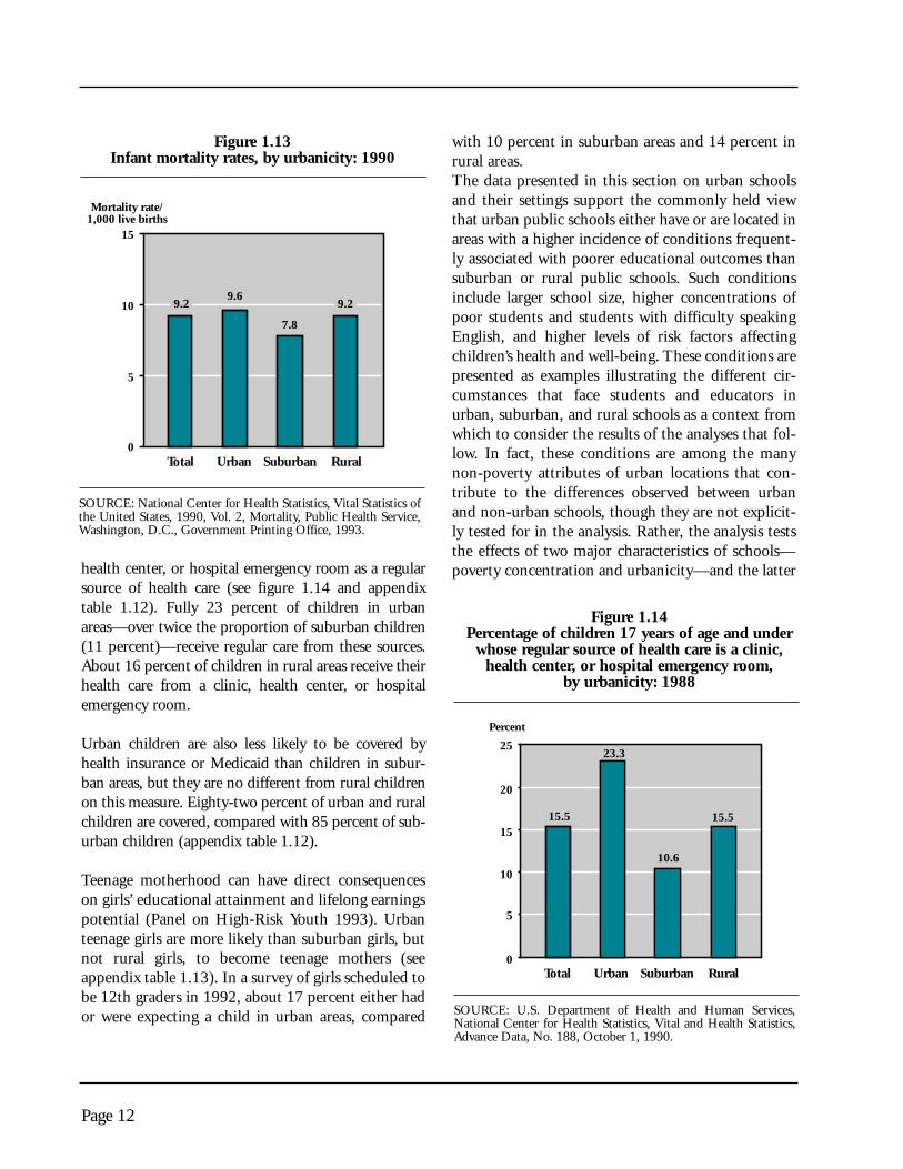
health center, or hospital emergency room as a regularsource of health care (see figure 1.14 and appendixtable 1.12). Fully 23 percent of children in urbanareas—over twice the proportion of suburban children(11 percent)—receive regular care from these sources.About 16 percent of children in rural areas receive theirhealth care from a clinic, health center, or hospitalemergency room.
Urban children are also less likely to be covered byhealth insurance or Medicaid than children in subur-ban areas, but they are no different from rural childrenon this measure. Eighty-two percent of urban and ruralchildren are covered, compared with 85 percent of sub-urban children (appendix table 1.12).
Teenage motherhood can have direct consequenceson girls’ educational attainment and lifelong earningspotential (Panel on High-Risk Youth 1993). Urbanteenage girls are more likely than suburban girls, butnot rural girls, to become teenage mothers (seeappendix table 1.13). In a survey of girls scheduled tobe 12th graders in 1992, about 17 percent either hador were expecting a child in urban areas, compared
with 10 percent in suburban areas and 14 percent inrural areas.The data presented in this section on urban schoolsand their settings support the commonly held viewthat urban public schools either have or are located inareas with a higher incidence of conditions frequent-ly associated with poorer educational outcomes thansuburban or rural public schools. Such conditionsinclude larger school size, higher concentrations ofpoor students and students with difficulty speakingEnglish, and higher levels of risk factors affectingchildren’s health and well-being. These conditions arepresented as examples illustrating the different cir-cumstances that face students and educators inurban, suburban, and rural schools as a context fromwhich to consider the results of the analyses that fol-low. In fact, these conditions are among the manynon-poverty attributes of urban locations that con-tribute to the differences observed between urbanand non-urban schools, though they are not explicit-ly tested for in the analysis. Rather, the analysis teststhe effects of two major characteristics of schools—poverty concentration and urbanicity—and the latter
Page 12
Mortality rate/1,000 live births
9.2
7.8
9.69.2
Total Urban Suburban Rural
15
10
5
0
Figure 1.13Infant mortality rates, by urbanicity: 1990
SOURCE: National Center for Health Statistics, Vital Statistics ofthe United States, 1990, Vol. 2, Mortality, Public Health Service,Washington, D.C., Government Printing Office, 1993.
Percent
0
5
10
15
20
25
15.5
10.6
23.3
15.5
Total Urban Suburban Rural
Figure 1.14Percentage of children 17 years of age and under
whose regular source of health care is a clinic,health center, or hospital emergency room,
by urbanicity: 1988
SOURCE: U.S. Department of Health and Human Services,National Center for Health Statistics, Vital and Health Statistics,Advance Data, No. 188, October 1, 1990.

can be said to serve as a proxy for all of the attribut-es of urban settings.
The data presented in this section and the researchreviewed in this chapter lead one to expect that urbanstudents would indeed have poorer education out-comes than the students in other schools. Chapter 2examines this question using the analytical approach,data sources, and definitions described below.
Approach
In addressing the question: Are urban schools differ-ent? one might simply report the differences observedbetween urban and other schools. But since urbanschools have higher concentrations of low incomestudents and the relationship between such concen-trations and less desirable education outcomes iswell-documented (see section on previous research),the question becomes: Are urban schools differentafter accounting for differences in the concentrationof poverty between schools in different locations?Further, if there is a relationship between an urbanlocation and the outcomes separate from the effect ofhigher poverty concentration, do these two charac-teristics combine to produce an additional effect, orinteraction, for urban schools with the highest povertyconcentrations? That is, are conditions and outcomesfor students in these schools compared to other schoolsdifferent than predicted because of a compoundingeffect of an urban location and high concentrations oflow income students in the school?
The basic approach, then, is to take two salientcharacteristics of schools—location and povertyconcentration—and test their independent andjoint relationship to indicators of education outcomesin chapter 2, family background and afterschoolexperiences in chapter 3, and school experiences inchapter 4.
The first area in which urban schools are comparedwith other schools is education outcomes. This analysisestablishes whether there are, in fact, differences betweenthe academic achievement, educational attainment, andeconomic outcomes of students who attended urban
public schools and other students. Differences in schoolexperiences are believed to have long-term effects onthe students’ postsecondary and career opportunities,and their ability to maintain a livelihood. In order tocapture these effects, longitudinal data are used that fol-low students who attended secondary school in differentlocations through their postsecondary and labor marketexperiences. The outcomes of students are compared notonly while they are in school but also at several mile-stones thereafter. Then, the family background factorsand school experiences that might be related to the dif-ferent outcomes are analyzed, and reported on at thetime the students were in school, which for most wasduring the 1980s.
In conducting the analysis for this report, four basicsteps were used, each of which answers a specific question:
1) Are urban schools different from other schools?That is, do urban students have different out-comes and experiences than suburban or ruralstudents?
2) Are schools with high poverty concentrationsdifferent from those with lower poverty concen-trations? That is, do students from schools withhigh poverty concentrations have different out-comes and experiences than students from otherschools?
3) Are urban schools different from other schoolsafter taking into account the poverty concentra-tion of the school? That is, is an urban schoollocation related to the different outcomes andexperiences of students in urban schools, aboveand beyond the fact that they have higher con-centrations of poor students?
4) Are urban high poverty schools different thanthe combination of the effects of an urban loca-tion and a high poverty concentration wouldpredict? That is, does the combination of anurban and high poverty setting interact so thatthe outcomes and experiences of students inthose settings are different than predicted? And,are urban high poverty schools different from
Page 13

other high poverty schools? Is high poverty con-centration in an urban setting different than it isin other settings?
Analysis of variance is the primary statistical test usedto answer these questions. Although hierarchical linearmodeling was considered as a possible basic analyticaltool because it has some technical advantages whenanalyzing data from two levels (student-level andschool-level, in the present case), it was decided thatanalysis of variance was preferable for two reasons.First, results from analysis of variance are more directlylinked to the research questions and can be more easilypresented to a general audience. Second, even if hierar-chical linear modeling had been the analysis of choice,it would have been applicable to some, but not all, ofthe data sets that are used in the report. It seemedpreferable to use a single analytical method throughoutthe report.
There are four models that correspond to the fourresearch questions stated above (see Appendix B for for-mulas and notation for the models). Data are presentedin three figures for each indicator in the report.
1) Model 1 tests the overall effect of urbanicity. Ifthe overall test is statistically significant, it teststhe difference between urban and suburbanschools, and between urban and rural schools.The data by urbanicity are presented in a bargraph in the first figure of each indicator.
2) Model 2 tests the overall effect of povertyconcentration. If the overall test is statisticallysignificant, model 2 tests the differencebetween students in schools with the highestpoverty concentration and students in schoolsat the three other levels of poverty concentration.Data by poverty concentration are presented in aline graph in the second figure for each indicator.
3) Model 3 tests the overall effect of urbanicity,controlling for differences in poverty concentra-tion. If the overall test is statistically significant,model 3 tests the difference between urban and
suburban students, controlling for poverty con-centration, and the difference between urbanand rural students, controlling for poverty con-centration.
4) Model 4 tests the overall effect of the interactionbetween urbanicity and poverty concentration. Ifthe overall test is statistically significant, model 4tests whether the difference between urban andother schools at the highest poverty concentra-tion is the same as the difference between urbanand other schools at lower levels of poverty con-centration. In addition, the difference betweenurban high poverty schools and other highpoverty schools is tested for significance.
The data on urbanicity by poverty concentration relatedto models 3 and 4 are represented in the third figure ofeach indicator. Although there are many possible patternsfor this figure, the following sample figures illustrate insimplified terms the way the data would appear if theyperfectly represented the effects that this analysis tests.The reader may compare these figures with the actualdata presented in the figures of the report.
Figure 1 indicates an effect of poverty concentrationbut no urbanicity effect when poverty concentration isheld constant. That is, the differences between urbanand other schools for variable Y are explained by thehigher concentration of poor students in urban schools.The difference between urban and other schools with
Page 14
Yi
Low High
suburban
rural
urban
Poverty concentrationPoverty concentration
suburbanruralurban
Low High
Yi
Figure 1
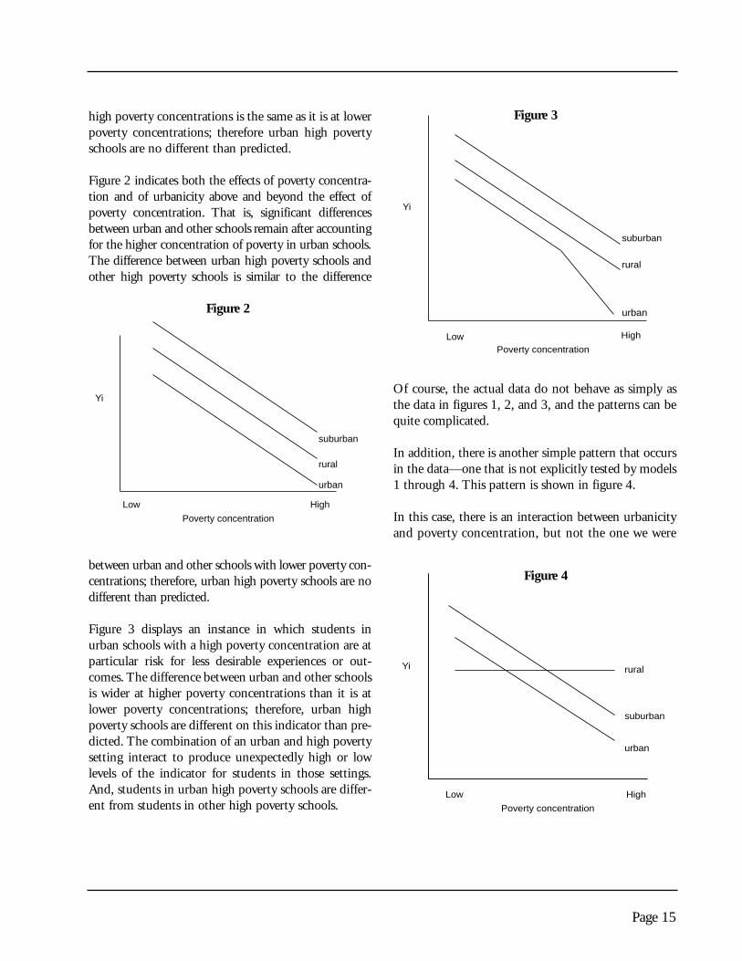
high poverty concentrations is the same as it is at lowerpoverty concentrations; therefore urban high povertyschools are no different than predicted.
Figure 2 indicates both the effects of poverty concentra-tion and of urbanicity above and beyond the effect ofpoverty concentration. That is, significant differencesbetween urban and other schools remain after accountingfor the higher concentration of poverty in urban schools.The difference between urban high poverty schools andother high poverty schools is similar to the difference
between urban and other schools with lower poverty con-centrations; therefore, urban high poverty schools are nodifferent than predicted.
Figure 3 displays an instance in which students inurban schools with a high poverty concentration are atparticular risk for less desirable experiences or out-comes. The difference between urban and other schoolsis wider at higher poverty concentrations than it is atlower poverty concentrations; therefore, urban highpoverty schools are different on this indicator than pre-dicted. The combination of an urban and high povertysetting interact to produce unexpectedly high or lowlevels of the indicator for students in those settings.And, students in urban high poverty schools are differ-ent from students in other high poverty schools.
Of course, the actual data do not behave as simply asthe data in figures 1, 2, and 3, and the patterns can bequite complicated.
In addition, there is another simple pattern that occursin the data—one that is not explicitly tested by models1 through 4. This pattern is shown in figure 4.
In this case, there is an interaction between urbanicityand poverty concentration, but not the one we were
Page 15
Yi
Low High
suburban
rural
urban
Poverty concentrationPoverty concentration
suburban
rural
urban
Low High
Yi
Figure 2
Yi
Low High
suburban
rural
urban
Poverty concentrationPoverty concentration
suburban
rural
urban
Low High
Yi
urban
Figure 3
Yi
Lo Hi
suburban
rural
urban
Yi
Low gh
Poverty concentrationPoverty concentration
suburban
rural
urban
Low High
Yi
Figure 4

explicitly looking for in model 4. In fact, what isinteresting is the lack of an overall effect of povertyconcentration on rural schools compared with a quitemarked effect for urban and suburban schools. That is,what is of interest here is the overall effect of povertyconcentration for rural schools, rather than the simplecontrast between high poverty concentration and lowpoverty concentration schools. A model was developedto test whether the slopes of the lines relating thepoverty concentration with the measure of interest inurban, suburban, and rural schools differed from oneanother, and for rural schools, to test whether it differsfrom zero.
The above discussion describes the research questionsposed in this report and the methodology used to sup-ply the answers. It is important to alert the reader to thelimitations of the analysis in this report.
• This report does not control for individualstudent-level background. Research has oftenshown that effects attributed to social compositionor context often diminish when controls for indi-vidual background are added. The measure ofschool poverty concentration (the percentage ofstudents in the school receiving free or reducedprice lunch) is intertwined with a measure of stu-dent background, since it is the aggregation ofindividual students’ poverty status. Indicators offamily background of students that are related toeducation outcomes are presented in chapter 3.
• The analysis in this report does not determine therelative strength of the relationship of urbanicity orschool poverty concentration to the indicators; itsimply tests whether differences by urbanicityremain after taking into account differences inpoverty concentration. Further, the analysis doesnot determine how much of the differencebetween urban and other schools can be attributedto urbanicity or poverty concentration.
• A finding that school urbanicity or povertyconcentration is related to a particular studentoutcome or experience does not suggest that
these school characteristics caused that out-come or experience. It only suggests that thereis a statistical association between urbanicity orpoverty concentration and the outcome orexperience. If it is found that an urban schoollocation matters, this suggests that the constel-lation of characteristics that are currentlyfound in urban areas is related to the outcomeor experience, not necessarily location itself.“Urban” in this context stands for all the char-acteristics of urban areas, as is the case for“suburban” and “rural.” If it is found that anurban location matters even when accountingfor higher urban poverty concentrations, thissuggests that there are additional non-povertyattributes of urban areas that are related to theindicator.
• The analysis does not estimate causal relation-ships between the family background and schoolexperiences of students and their educationoutcomes. However, the student backgroundand school experiences indicators presentedwere considered important, both in the researchliterature and in initial analyses demonstratingimportant differences by school urbanicity andpoverty concentration (see technical notes, appen-dix C). Further, the analysis does not determinethe relative importance of family backgroundcompared with school-level factors in affectingstudent outcomes. Rather, the analysis is primarilydescriptive of student outcomes, family back-ground, and school experiences, and how theyvary across school locations and levels of schoolpoverty concentration.
Sources
This report describes public school students and theirenvironments, and their educational and economicoutcomes in the late 1980s to 1990. The data sourcesand definitions of poverty and urbanicity for each dataset used in this report are described in detail in theappendices and in the introductions to each chapter.The following provides a summary.
Page 16

The contextual data provided in the section of thischapter entitled “The Setting: Urban Schools andCommunities” have been calculated by the authorsfrom the U.S Bureau of the Census’ CurrentPopulation Surveys of March and October 1980 and1990, and November 1979 and 1989; the NationalCenter for Education Statistics’ 1987–88 Schools andStaffing Survey (SASS), and the National EducationLongitudinal Study of 1988 (NELS:88); the U.S.Department of Justice, Bureau of Justice Statistics,National Crime Victimization Survey; and theNational Center for Health Statistics, Vital Statistics ofthe United States 1990, and the 1988 National HealthInterview Survey.
The indicators of education outcomes described inchapter 2 are derived from three nationally representa-tive data sets. Achievement data for 8th and 10thgraders come from NELS:88, which assessed a sampleof 8th graders in 1988 and reassessed them in 1990when most of them were in the 10th grade. Theachievement of 10th graders in 1990 is compared withthose in 1980 using a comparable assessment that waspart of the High School and Beyond Study (HS&B).The third follow-up survey of HS&B, which surveyed1980 sophomores in 1986 (4 years after most wouldhave finished high school), is the source of data on highschool completion; the 1990 follow-up of the NationalLongitudinal Survey of Youth (NLSY), which surveyedyoung adults ages 25-32, is the source of data for post-secondary completion and for all the measures ofeconomic outcomes. Thus, the student outcomesdescribed in chapter 2 refer to data gathered from 1980to 1990.
Chapters 3 and 4 describe the family, afterschool, andschool experiences of students during the same timeperiod. The indicators of family background and after-school activities that are presented in chapter 3 arederived from the NELS:88 base year survey of 8thgraders in 1988 and the first follow-up survey of 10thgraders in 1990. The data sources for school experi-ences in chapter 4 are the same two NELS:88 surveys,as well as the 1987–88 Schools and Staffing Survey.High school transcript data are from the National
Assessment of Educational Progress (NAEP) HighSchool Transcript Study of 1990.
Definitions of Urbanicity and Poverty Concentration
The definitions of urbanicity and poverty concentra-tion vary somewhat across the sources of data.Although every effort was made to use comparable datawhen possible, some differences should be noted.
The categories used in this report to denote theurbanicity of a school are urban, suburban, and rural.For all surveys except SASS, these correspond to U.S.Bureau of the Census classifications of the schoollocation. Schools classified as urban are located incentral cities of Metropolitan Statistical Areas(MSAs); schools classified as suburban are locatedwithin the area surrounding a central city within theMSA; and schools classified as rural are outside of anMSA. Urban schools were located in central cities ofall sizes, as defined by the Census Bureau. For the1987–88 SASS, the school administrator was askedto assign one of ten residence categories to his or herschool, and these have been collapsed into three cat-egories for this report as follows: urban schools locatedin cities of 50,000 people or more; suburban schoolslocated in the suburbs of cities of 50,000 or more;and rural schools, including rural or farming com-munities, towns of less than 50,000 people that are notsuburbs of a larger city, and Indian reservations.
Information on school poverty concentration for eachsurvey is obtained from school administrators in whichthey report the percentage of students in the schoolwho receive free or reduced price lunch (for the NELS,SASS, and NAEP surveys), or report the percentage inthe school who are classified as disadvantaged (for theHS&B and NLSY surveys). The term “disadvantaged”was more commonly used at the time students were inhigh school in the late 1970s and early 1980s whenthey were surveyed as part of the HS&B and NLSYstudies, and can have several interpretations (Natrielloet al. 1990; Ralph 1992). School administrators werelikely to have interpreted “disadvantaged” to mean stu-dents who would be eligible for services under Chapter
Page 17
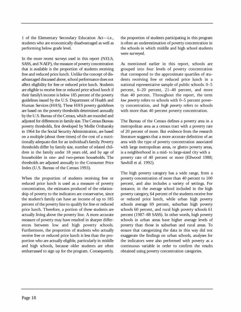
1 of the Elementary Secondary Education Act—i.e.,students who are economically disadvantaged as well asperforming below grade level.
In the more recent surveys used in this report (NELS,SASS, and NAEP), the measure of poverty concentrationthat is available is the proportion of students receivingfree and reduced price lunch. Unlike the concept of dis-advantaged discussed above, school performance does notaffect eligibility for free or reduced price lunch. Studentsare eligible to receive free or reduced price school lunch iftheir family’s income is below 185 percent of the povertyguidelines issued by the U.S. Department of Health andHuman Services (HHS). These HHS poverty guidelinesare based on the poverty thresholds determined annuallyby the U.S. Bureau of the Census, which are rounded andadjusted for differences in family size. The Census Bureaupoverty thresholds, first developed by Mollie Orshanskyin 1964 for the Social Security Administration, are basedon a multiple (about three times) of the cost of a nutri-tionally adequate diet for an individual’s family. Povertythresholds differ by family size, number of related chil-dren in the family under 18 years old, and by age ofhouseholder in one- and two-person households. Thethresholds are adjusted annually to the Consumer PriceIndex (U.S. Bureau of the Census 1993).
When the proportion of students receiving free orreduced price lunch is used as a measure of povertyconcentration, the estimates produced of the relation-ship of poverty to the indicators are conservative, sincethe student’s family can have an income of up to 185percent of the poverty line to qualify for free or reducedprice lunch. Therefore, a portion of these students areactually living above the poverty line. A more accuratemeasure of poverty may have resulted in sharper differ-ences between low and high poverty schools.Furthermore, the proportion of students who actuallyreceive free or reduced price lunch is less than the pro-portion who are actually eligible, particularly in middleand high schools, because older students are oftenembarrassed to sign up for the program. Consequently,
the proportion of students participating in this programis often an underestimation of poverty concentration inthe schools in which middle and high school studentswere surveyed.
As mentioned earlier in this report, schools aregrouped into four levels of poverty concentrationthat correspond to the approximate quartiles of stu-dents receiving free or reduced price lunch in anational representative sample of public schools: 0–5percent, 6–20 percent, 21–40 percent, and morethan 40 percent. Throughout the report, the termlow poverty refers to schools with 0–5 percent pover-ty concentration, and high poverty refers to schoolswith more than 40 percent poverty concentration.
The Bureau of the Census defines a poverty area in ametropolitan area as a census tract with a poverty rateof 20 percent of more. But evidence from the researchliterature suggests that a more accurate definition of anarea with the type of poverty concentration associatedwith large metropolitan areas, or ghetto poverty areas,is a neighborhood in a mid- to large-sized city with a poverty rate of 40 percent or more (Ellwood 1988;Sawhill et al. 1992).
The high poverty category has a wide range, from apoverty concentration of more than 40 percent to 100percent, and also includes a variety of settings. Forinstance, in the average school included in the highpoverty category, 64 percent of the students receive freeor reduced price lunch, while urban high povertyschools average 69 percent, suburban high povertyschools 60 percent, and rural high poverty schools 61percent (1987–88 SASS). In other words, high povertyschools in urban areas have higher average levels ofpoverty than those in suburban and rural areas. Toensure that categorizing the data in this way did notexaggerate the findings on urban schools, analyses forthe indicators were also performed with poverty as acontinuous variable in order to confirm the resultsobtained using poverty concentration categories.
Page 18

There is a commonly held perception that children inurban public schools exhibit a pattern of academicfailure that leads to dropping out of school and later,failure to obtain and maintain a livelihood. This chap-ter uses nationally representative data and statisticalanalyses to test this perception.
Chapter 1 reviewed previous research and contextualdata suggesting that students in urban public schools—and especially those in urban schools with highconcentrations of disadvantaged students—would beexpected to compare less favorably on achievement,educational attainment, and on indicators of economicstatus than students from other schools. This chapterexamines the available data for each of these three areas.Further, given that urbanicity is confounded withpoverty, it explores whether the urbanicity of a schoolcontinues to be related to student outcomes when thehigher concentration of poverty in urban schools isconsidered. The analysis uses data on a battery of indi-cators of achievement, attainment, and economicoutcomes, and these data are subjected to statisticaltests to determine the relationship between these out-comes and urbanicity, controlling for poverty and incombination with poverty.
The approach used for the analysis in this chapter willserve as a model for the chapters that follow. Studentsin national surveys are grouped according to the urban-icity and the level of poverty concentration in theschools they attended, using comparable definitions ofurbanicity and poverty concentration. In the achieve-ment section, poverty is measured as the percent ofstudents receiving free and reduced price lunch, whilein the attainment and economic outcomes sections,which use data from older surveys, it is measured as thepercentage identified as “disadvantaged” by a schooladministrator.
The data for each outcome measure were subjected toa series of statistical tests using analysis of variance
(see chapter 1 and appendix B) to determine specif-ically:
1) how the performance of urban students, overall,compared to suburban or rural students;
2) how the performance of students in schoolswith higher poverty concentrations comparedto students in schools with lower poverty con-centrations;
3) how the performance of students from urbanschools compared if the concentration of pover-ty in their schools was considered; and finally
4) how the performance of students in urbanschools with the highest poverty concentrationscompared to those in similar schools in suburbanand rural areas, and whether they suffered anyadditional penalty on achievement tests, inattaining education, and in achieving economicwell-being that was related to the interaction, orcompounding effect, of an urban and a highpoverty setting.
The results of this last test are expressed by the phrasegreater than predicted when the difference betweenurban high poverty and other high poverty schools islarger than would be predicted from the combinedeffects of urbanicity and poverty concentration, or nodifferent than predicted when the difference can beexplained by these two main effects.
Chart 2.1 summarizes the results of the analyses ofeducation outcomes, grouped into three sections—student achievement, educational attainment, andeconomic outcomes. The indicators of studentachievement are mathematics and reading test com-posite scores for 8th- and 10th-grade students, and theoverall change in 10th graders’ mathematics scoresfrom 1980 to 1990. Rates of on-time high school
Page 19
Chapter 2
Education Outcomes
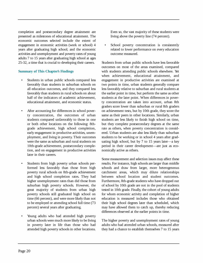
completion and postsecondary degree attainment arepresented as milestones of educational attainment. Theeconomic outcomes selected include the extent ofengagement in economic activities (work or school) 4years after graduating high school; and the economicactivities and unemployment and poverty rates of youngadults 7 to 15 years after graduating high school at ages25-32, a time that is crucial to developing their careers.
Summary of This Chapter’s Findings
• Students in urban public schools compared lessfavorably than students in suburban schools onall education outcomes, and they compared lessfavorably than students in rural schools on abouthalf of the indicators of academic achievement,educational attainment, and economic status.
• After accounting for differences in school pover-ty concentration, the outcomes of urbanstudents compared unfavorably to those in oneor both other locations on the following: 8th-grade achievement, high school completion,early engagement in productive activities, unem-ployment, and living in poverty. Their outcomeswere the same as suburban and rural students on10th-grade achievement, postsecondary comple-tion, and on engagement in productive activitieslater in their careers.
• Students from high poverty urban schools per-formed less favorably than those from highpoverty rural schools on 8th-grade achievementand high school completion rates. They hadhigher unemployment rates than did those fromsuburban high poverty schools. However, thegreat majority of students from urban highpoverty schools still graduated high school ontime (66 percent), and were more likely than notto be employed or attending school full time (73percent) several years after graduating.
• Young adults who had attended high povertyurban schools were much more likely to be livingin poverty later in life than those who hadattended high poverty schools in other locations.
Even so, the vast majority of these students wereliving above the poverty line (74 percent).
• School poverty concentration is consistentlyrelated to lower performance on every educationoutcome measured.
Students from urban public schools have less favorableoutcomes on most of the areas examined, comparedwith students attending public schools elsewhere. Yetwhen achievement, educational attainment, andengagement in productive activities are examined attwo points in time, urban students generally compareless favorably relative to suburban and rural students atthe earlier point in time, but perform the same as otherstudents at the later point. When differences in pover-ty concentration are taken into account, urban 8thgraders score lower than suburban or rural 8th graderson achievement tests, but by 10th grade, they score thesame as their peers in other locations. Similarly, urbanstudents are less likely to finish high school on time,but they complete postsecondary degrees at the samerate as others, when poverty concentration is consid-ered. Urban students are also less likely than suburbanstudents to be working or in school 4 years after grad-uating high school, but by 7 to 15 years later—a keyperiod in their career development—are just as eco-nomically active as others.
Some measurement and selection issues may affect theseresults. For instance, high schools are larger than middleschools and draw from larger, more heterogeneouscatchment areas, which may dilute relationshipsbetween school location and student outcomes.Furthermore, 8th-grade students who have dropped outof school by 10th grade are not in the pool of studentstested in 10th grade. Finally, the cohort of young adultsfor whom economic activity and completion of highereducation is measured includes those who obtainedtheir high school degrees later than scheduled, whichmay have allowed them to catch up, thereby reducingdifferences observed at the earlier points in time.
The higher poverty and unemployment rates of youngadults who had attended urban schools, measured afterthey had a chance to establish themselves 7 to 15 years
Page 20

after they would normally have graduated from highschool, does suggest that urban students are more like-ly to have periods of marginal economic existence thanstudents from schools in other locations. The size of thegap between students from urban schools and others onthese two indicators is large. It should be noted thatthis study did not account for differences by location inlabor markets at the time of the surveys. If the surveyrespondents were living in areas with higher povertyand unemployment rates at the time their progress wasmeasured, these factors would also affect the respon-dents’ status.
Students who attended schools that were both urbanand had a high concentration of poor or disadvantagedstudents were at a much higher risk of living in pover-ty later in life than others. Compared with studentsfrom schools in rural areas with similarly high propor-tions of poor or disadvantaged students, theyperformed less well on 8th-grade achievement tests andwere less likely to complete high school. Moreover, theyhad higher unemployment rates than those from simi-lar suburban schools. But on the other indicators ofachievement, attainment, and economic success, stu-dents from urban high poverty schools performedcomparably to those from high poverty schools in otherlocations. In fact, high poverty schools in all locationswere similar on half of the indicators, including again,
those at a later point in the life course. This suggests thepossibility that the effects of high poverty concentra-tion may diminish over time for certain aspects of thesestudents’ lives. The relationship between poverty andthe outcomes presented here may be underestimated bythe less accurate measure of poverty used in older sur-veys from which some of the data were drawn.
In no case were the outcomes of students in urban highpoverty schools different than predicted: the less favor-able outcomes observed for these students could bepredicted from the combined effects of an urban settingand a high poverty setting. Thus, there was no evidencethat they may have suffered any additional penalty relat-ed to the interaction, or compounding effect, of the two.
This chapter focuses on how the outcomes of studentsfrom urban high poverty schools differed from those oftheir counterparts in other locations. The evidence thatthese students achieve less, attain less education, andfare less well economically than other students is consis-tent with prior research and the demographic, health,and community risk factors outlined in chapter 1.However, as mentioned previously, the great majority ofthese students still graduated high school on time (66percent) and, several years later, were more likely thannot to be employed or in school (73 percent) and livingabove the poverty line (74 percent).
Page 21

Are Urban Are High Are Urban Are Urban HighSchools Poverty Schools Schools Poverty SchoolsDifferent? Different?* Different after Different from
Accounting for Other HighPoverty Poverty Schools?Concentration?
Are Urban HighPoverty SchoolsDifferent than
INDICATOR Predicted?
I. STUDENT ACHIEVEMENT
8th-Grade Yes, Yes, Yes, Yes,Composite urban lower than high poverty lower urban lower than same as suburban,Score suburban and than most others others lower than rural high
rural poverty
No differentthan predicted
10th-Grade Yes, Yes, No, No,Composite urban lower than high poverty lower urban same as same as otherScore suburban, same than all others others high poverty
as ruralNo differentthan predicted
1980-1990 Yes, NA NA NAChange in urban lower than10th-Grade others in 1980,Math Score lower than
suburban in 1990
II. EDUCATIONAL ATTAINMENT
High School Yes, Yes, Yes, Yes,Completion urban lower than high poverty lower urban lower than lower than rural,
suburban and than all others others same as suburbanrural high poverty
No differentthan predicted
Page 22
CHART 2.1—SUMMARY OF RESULTS: EDUCATION OUTCOMES

Are Urban Are High Are Urban Are Urban HighSchools Poverty Schools Schools Poverty SchoolsDifferent? Different?* Different After Different From
Accounting for Other HighPoverty Poverty Schools?Concentration?
Are Urban HighPoverty SchoolsDifferent Than
INDICATOR Predicted?
Postsecondary Yes, Yes, No, No,Degree urban lower than high poverty lower urban same as same as other Attainment suburban, same than most others others high poverty
as rural
No differentthan predicted
III. ECONOMIC OUTCOMES
Early Yes, Yes, Yes, No,Productive urban lower than high poverty lower urban lower than same as otherActivity suburban, same than all others suburban high poverty
as ruralNo differentthan predicted
Later Yes, Yes, No, No,Productive urban lower than high poverty lower urban same as same as otherActivity suburban, same than most others high poverty
as rural othersNo differentthan predicted
Unemployment Yes, Yes, Yes, Yes,urban higher than high poverty lower urban higher than higher than suburban,suburban and than all others others same as rural high rural poverty
No differentthan predicted
Poverty Yes, Yes, Yes, Yes,urban higher than high poverty higher urban higher than higher thansuburban and than all others others other high povertyrural
No differentthan predicted
Page 23
*Poverty at the school level is measured by the percentage of students receiving free or reduced-price lunch in the student achievementsection and the percentage identified as “disadvantaged” by school administrators in the educational attainment and economic outcomessection.

Student achievement is a primary measure of schoolsuccess. Parents and school officials alike interprettest scores as a reflection of whether students, as wellas the educational system, are performing satisfacto-rily (Special Study Panel on Education Indicators1991).
The challenge in measuring educational achievementnationally is to measure achievement consistentlyacross diverse populations of students throughout thecountry, who are exposed to a wide range of teachingquality and practices, school resources, and curricula.National assessments have been developed to enablenationwide comparisons of the performance of studentswho are educated in widely different circumstances.
This section discusses the findings from two suchlongitudinal surveys (surveys that follow the sameindividuals over time), which contain national assess-ments as part of the survey. First, the mathematicsand reading test scores of 8th graders in 1988 and10th graders in 1990 are presented from an assess-ment administered as part of the National EducationLongitudinal Study of 1988 (NELS:88). Then, theperformance of the same 10th graders in math in1990 is compared to that of 10th graders in 1980,who were assessed in a comparable test as part of theHigh School and Beyond Study (HS&B), to deter-mine if the performance of students in urban,suburban, and rural schools has changed over thedecade.
The analysis of the measures of student achievementaddressed in this section will be presented in a stan-dard order. First, the average scores of public schoolstudents in urban locations will be compared to theircounterparts in suburban and rural locations.Second, the average scores of students who attendedschools with high concentrations of poverty will becompared to those who attended schools with lowerconcentrations of poverty. Third, the students aregrouped according to the urbanicity and the level of
poverty in their schools, in order to make compar-isons between students attending schools with similarconcentrations of poor students (measured as thosereceiving free or reduced price lunch). Finally, stu-dents from urban high poverty schools are comparedto students from high poverty schools in other locations.
In this analysis, statistical tests are performed todetermine whether the differences in the averagescores of the groups being compared are statisticallysignificant, rather than due to chance. All differencesthat are reported are statistically significant.
Findings
• Urban 8th graders scored lower on achieve-ment tests than suburban or rural 8th graders,even when the higher poverty concentration ofurban public schools was taken into account.
• Urban 10th graders scored the same as rural10th graders, but scored lower than suburban10th graders. However, this was not related toan urban location; rather, it was due to thehigher poverty concentration in urban areas.
• Students in urban high poverty schools achievedat about the same level as would be predictedfrom the combination of an urban and highpoverty setting. In fact, in urban high povertyschools, 8th graders scored about the same asthose in suburban high poverty schools, and10th graders scored about the same as those inrural high poverty schools and suburban schoolswith the highest and next to highest levels ofpoverty concentration. However, 8th graders inurban high poverty schools scored lower thanthose in rural locations.
• The concentration of poverty in a school hadan important relationship to achievement—asthe proportion of poor students in a school
Page 24
Student Achievement

increased, student performance on achieve-ment tests in both 8th and 10th grades and inevery location generally decreased.
• Between 1980 and 1990, the mathematicsachievement of students in public schools in
every location increased moderately. However,there were no meaningful differences in theamount of increase across locations. Urban stu-dents scored lower in mathematics than bothsuburban and rural students in 1980, but lowerthan only suburban students in 1990.
Page 25
STUDENT ACHIEVEMENT

Are urban schools different? In 1988, the academicachievement of 8th graders in urban public schoolslagged behind that of their peers in suburban and ruralschools (figure 2.1). In a national test of math and read-ing achievement, students scored a mean of 49.5 overall,but urban 8th graders scored 47, or at the 38th per-centile, while suburban students scored 51 (at the 54thpercentile), and rural students scored 49 (at the 46thpercentile).2
Are high poverty schools different? Students in schoolswith high poverty concentrations also achieved at lowerlevels than students in most other schools. Students inschools with the highest concentration of povertyscored an average of 45 (at the 31st percentile), while
students in schools with the lowest concentration ofpoverty scored 53 (at the 62nd percentile) (figure 2.2).
Are urban schools different after accounting for povertyconcentration? The low performance of urban studentscannot be attributed to the poverty concentration of theirschools alone. They still would have performed less well,on average, than students in other areas, even if theirschool had the same level of poverty concentration asschools in other areas.
Is 8th-grade student achievement in urban high pover-ty schools lower than predicted? Students in urbanschools with high concentrations of poverty had lowercomposite scores than students in similar schools in rural
Page 26
STUDENT ACHIEVEMENT
Academic Achievement of 8th Graders
Test score
Total Urban Suburban Rural0
40
50
55
50.849.4
47.0
49.5
45
School poverty concentration(percent)
0 to 5 6 to 20 21 to 40 Over 400
40
50
55
45
Test score
Figure 2.1Average standardized test
composite scores of 8th-grade students, by urbanicity: 1988
Figure 2.2Average standardized test
composite scores of 8th-grade students, by school poverty concentration: 1988
SOURCE: U.S. Department of Education, National Center forEducation Statistics, National Education Longitudinal Study of1988, Base Year Survey.
SOURCE: U.S. Department of Education, National Center forEducation Statistics, National Education Longitudinal Study of1988, Base Year Survey.
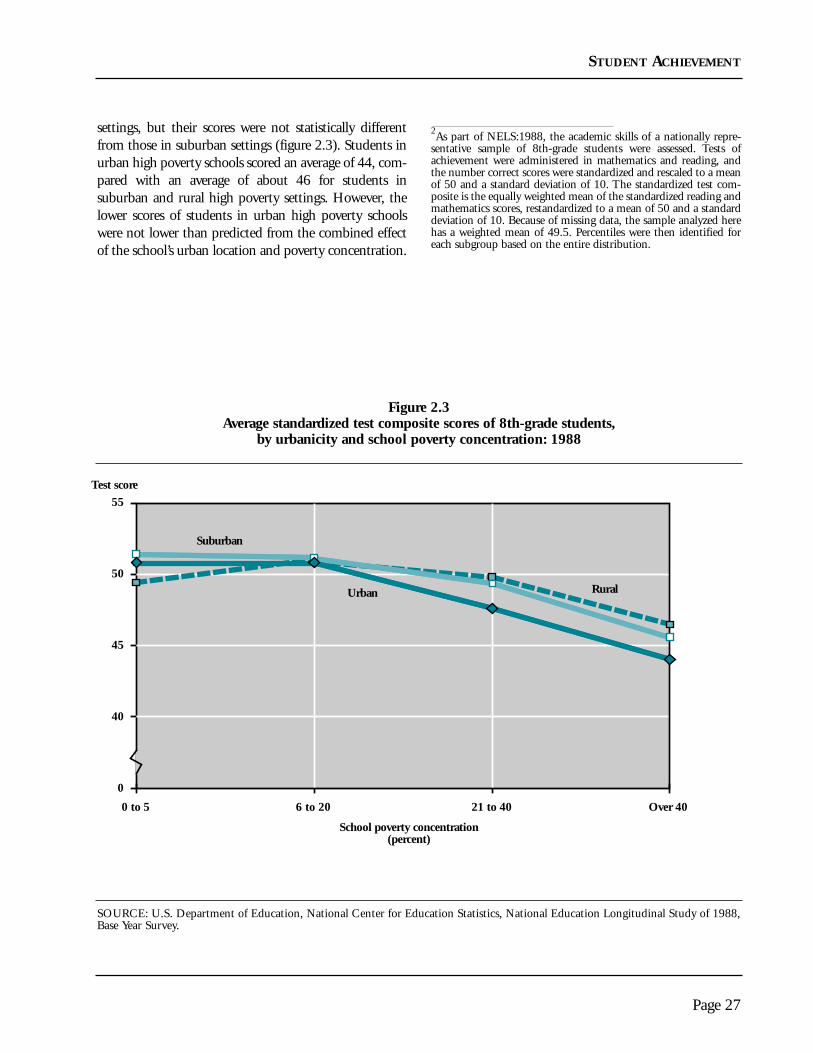
settings, but their scores were not statistically differentfrom those in suburban settings (figure 2.3). Students inurban high poverty schools scored an average of 44, com-pared with an average of about 46 for students insuburban and rural high poverty settings. However, thelower scores of students in urban high poverty schoolswere not lower than predicted from the combined effectof the school’s urban location and poverty concentration.
2As part of NELS:1988, the academic skills of a nationally repre-sentative sample of 8th-grade students were assessed. Tests ofachievement were administered in mathematics and reading, andthe number correct scores were standardized and rescaled to a meanof 50 and a standard deviation of 10. The standardized test com-posite is the equally weighted mean of the standardized reading andmathematics scores, restandardized to a mean of 50 and a standarddeviation of 10. Because of missing data, the sample analyzed herehas a weighted mean of 49.5. Percentiles were then identified foreach subgroup based on the entire distribution.
Page 27
STUDENT ACHIEVEMENT
Figure 2.3Average standardized test composite scores of 8th-grade students,
by urbanicity and school poverty concentration: 1988
45
Test score
0 to 5 6 to 20 21 to 40 Over 40
Suburban
Urban Rural
0
40
50
55
School poverty concentration(percent)
SOURCE: U.S. Department of Education, National Center for Education Statistics, National Education Longitudinal Study of 1988,Base Year Survey.

Does the difference in achievement observed for urban8th graders remain in 10th grade? This section presentsevidence from the first follow-up of the same national-ly representative survey, NELS:88—but 2 years later in1990 when most of the 1988 8th graders were in 10thgrade. However, not all of the same 8th graders were inthis 10th-grade sample because some may have movedout of the country, dropped out of school, or repeateda grade. In addition, this 10th-grade sample has been“freshened” with 1990 10th graders who were not inthe 8th-grade sample in 1988 to make it nationally rep-resentative of all public school 10th graders in 1990.Again, the indicator presented is an overall average testcomposite score calculated from mathematics and read-ing test scores.3
Are urban schools different? Urban 10th graders scoredlower than their suburban counterparts on tests ofachievement in mathematics and reading (figure 2.4).They had a composite test score of about 49, while sub-urban students had an average score of 51. Urban scoreswere no different than rural scores.
Are high poverty schools different? As with 8thgraders, 10th-grade achievement was related to theconcentration of poverty in the school (figure 2.5).Students in schools with the highest concentration ofpoverty had the lowest level of achievement (scoring 45on average), whereas those in schools with the lowestpoverty concentration scored an average of 53. Just likethe 8th graders, the 10th graders in high poverty
Page 28
STUDENT ACHIEVEMENT
Academic Achievement of 10th Graders
Test score
Total Urban Suburban Rural0
40
50
55
51.2
49.348.850.0
45
School poverty concentration(percent)
0 to 5 6 to 20 21 to 40 Over 400
40
50
55
45
Test score
Figure 2.4Average standardized test
composite scores of 10th-grade students,by urbanicity: 1990
Figure 2.5Average standardized test
composite scores of 10th-grade students,by school poverty concentration: 1990
SOURCE: U.S. Department of Education, National Center forEducation Statistics, National Education Longitudinal Study of1988, First Follow-up Survey, 1990.
SOURCE: U.S. Department of Education, National Center forEducation Statistics, National Education Longitudinal Study of1988, First Follow-up Survey, 1990.
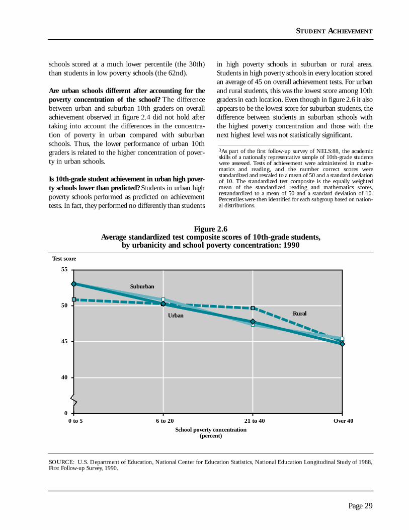
schools scored at a much lower percentile (the 30th)than students in low poverty schools (the 62nd).
Are urban schools different after accounting for thepoverty concentration of the school? The differencebetween urban and suburban 10th graders on overallachievement observed in figure 2.4 did not hold aftertaking into account the differences in the concentra-tion of poverty in urban compared with suburbanschools. Thus, the lower performance of urban 10thgraders is related to the higher concentration of pover-ty in urban schools.
Is 10th-grade student achievement in urban high pover-ty schools lower than predicted? Students in urban highpoverty schools performed as predicted on achievementtests. In fact, they performed no differently than students
in high poverty schools in suburban or rural areas.Students in high poverty schools in every location scoredan average of 45 on overall achievement tests. For urbanand rural students, this was the lowest score among 10thgraders in each location. Even though in figure 2.6 it alsoappears to be the lowest score for suburban students, thedifference between students in suburban schools withthe highest poverty concentration and those with thenext highest level was not statistically significant.
Page 29
STUDENT ACHIEVEMENT
Figure 2.6Average standardized test composite scores of 10th-grade students,
by urbanicity and school poverty concentration: 1990
45
Test score
0 to 5 6 to 20 21 to 40 Over 40
Suburban
Urban Rural
0
40
50
55
School poverty concentration(percent)
SOURCE: U.S. Department of Education, National Center for Education Statistics, National Education Longitudinal Study of 1988,First Follow-up Survey, 1990.
3As part of the first follow-up survey of NELS:88, the academicskills of a nationally representative sample of 10th-grade studentswere assessed. Tests of achievement were administered in mathe-matics and reading, and the number correct scores werestandardized and rescaled to a mean of 50 and a standard deviationof 10. The standardized test composite is the equally weightedmean of the standardized reading and mathematics scores,restandardized to a mean of 50 and a standard deviation of 10.Percentiles were then identified for each subgroup based on nation-al distributions.

STUDENT ACHIEVEMENT
The previous section compared the achievement ofurban 10th graders with their suburban and rural coun-terparts. The discussion in this section turns to whetherdifferences in achievement by school location havechanged over the decade of the 1980s.
The source of data is a mathematics test given to anationally representative sample of public high schoolsophomores in 1980 (from the HS&B Base YearSurvey), which has been equated to the test given to the1990 sample of sophomores from the NELS:88 FirstFollow-up Survey. (A composite score of mathematicsand reading achievement, used in the preceding analy-sis, is unavailable for both groups of sophomores.) The10th graders’ average number of correct responses iscompared according to the location of their school.4
Since the definitions of poverty used in the two surveyswere not comparable, comparisons could not be madeby school poverty concentration.
Overall, sophomores in 1990 were able to correctlyanswer about two more items than sophomores in1980 (figure 2.7). Students in all three locationsimproved their performance over the decade and exhib-ited similar levels of improvement. Urban 10th gradersanswered fewer items correctly than did their suburbanor rural counterparts in 1980. By 1990, urban studentsagain answered fewer items correctly than suburbanstudents, but there was no significant differencebetween their performance and that of rural students.Urban students in 1990 performed at about the samelevel as suburban students had in 1980.
Page 30
Did 10th-Grade Achievement Change Between 1980 and 1990?
Figure 2.7Average number correct in mathematics for 10th-grade students, by urbanicity: 1980 and 1990
Total Suburban RuralUrban
1980 1990
Number correct
0
20
25
30
35
40
29.7
33.733.9
37.234.9
31.7
33.235.6
SOURCE: U.S. Department of Education, National Center for Education Statistics, High School and Beyond, Base Year Survey, 1980,and the National Education Longitudinal Study of 1988, First Follow-up Survey, 1990.
4The data presented in this section are the estimated number of cor-rect items on the mathematics assessments of two surveys: the 1980HS&B Survey and NELS, 1990. The two assessments had enoughitems in common for them to be equated. Also, the number of cor-rect items is used in this analysis, rather than standardized scores, topreserve the observed differences in the two groups. Standardizingeach group's scores to have a mean of 50 and a standard deviation of10 would obscure such observed differences.

One of the most basic outcome measures of an educationsystem is the educational attainment—that is, the amountof education or credentials attained—of the students whopass through the system. The level of education that stu-dents complete has a strong and direct impact on theiremployment and earnings potential.
It has been well documented that rates of employmentare higher and more stable for those with higher educa-tional attainment. While 70 percent of men ages 25–34who did not complete high school were employed in1991, 85 percent of men of this same age group who hadcompleted high school were employed. Higher rates ofemployment were found among those who attended col-lege: 89 percent of those with 1–3 years of college wereemployed, as were 92 percent of those with 4 or moreyears of college. In addition, the employment rates of col-lege graduates remained stable during downturns in theeconomy over the last two decades, whereas they havedeclined for those with less education (U.S. Departmentof Education 1992).
Earnings are also strongly related to the level of educationattained. Individuals who have completed high schooland college earn more than those who have not. Forexample, white and black male high school graduates ages25–34 earned about 27 percent more in 1990 than thosewho had not completed high school. In 1990, white andblack males who had completed a college educationearned 42 and 66 percent more, respectively, than thosewho had completed no more than a high school degree.The differential returns to education are even more dra-matic for females (U.S. Department of Education 1992).
Educational attainment is related to the availability ofopportunities, as well as the academic abilities, financialresources, and persistence of the individual. In this report,two measures of educational attainment are presented attwo stages of completion that have a bearing on futureopportunities. These measures are 1) the rate at whichsophomores complete high school on time, from theHS&B survey; and 2) the rate at which young adults
complete any postsecondary degree, from the NationalLongitudinal Survey of Youth (NLSY). The measure ofschool poverty used in this section is the percentage ofstudents in the school who are reported to be “disadvan-taged” by school administrators, since this is the measureavailable in these two surveys.
The analysis described here will follow the same orderas it did in the achievement section. First, measures ofstudent attainment will be presented by urbanicity, fol-lowed by the level of concentration of disadvantagedstudents in the school, and by both characteristics com-bined. The statistical analysis presented in the previoussection will be used to determine how the urbanicityand concentration of disadvantaged students in theschool, separately and combined, are related to the edu-cational attainment of students in those schools.
Findings
• Urban public school students were less likely tograduate from high school on time than suburbanor rural students. This was related to the locationof the school apart from the higher concentrationof disadvantaged students in urban areas.
• Urban students were less likely to complete apostsecondary degree than suburban students.However, the differences appear to be related tothe concentration of disadvantaged students inpublic schools in urban areas, rather than location.
• Students from urban schools with the highestproportion of disadvantaged students graduatedfrom high school on time at rates that were lowerthan those in similar rural schools, but at ratesthat were not statistically different from similarsuburban schools. They obtained higher educa-tion degrees at about the same rates as those fromsuburban and rural schools with the same highlevel of disadvantaged students.
Page 31
Educational Attainment

Traditionally, one yardstick used to measure the out-comes of education has been students’ completion ofhigh school. This section looks at “on-time graduation”from high school, which is measured by the proportionof the high school sophomore class of 1980 who grad-uated with their class in 1982. The source of data forthe measure is the HS&B Third Follow-up Survey.
A small, but significant, proportion of students com-plete high school beyond the traditional graduationage. In fact, some do not complete until their late 20s.However, these students are not considered to be on-time graduates in the measure of completion used here.
Are urban schools different? Almost 82 percent of thestudents in the sophomore class of 1980 attending
public schools graduated on time with their classmates(figure 2.8). However, a smaller proportion of studentsin urban schools graduated on time compared with stu-dents in suburban or rural schools. Only 74 percent ofstudents from urban schools graduated on time com-pared with 84 percent of students in suburban schoolsand 83 percent of students in rural schools.
Are schools with high concentrations of disadvan-taged students different? Students from schools withfewer disadvantaged students were more likely tograduate on time than students from schools with largeproportions of disadvantaged students. Only 73 per-cent of students in the most disadvantaged schoolsgraduated on time compared with 80 percent or moreof students in other schools (figure 2.9).
Page 32
EDUCATIONAL ATTAINMENT
High School Completion
70
Percent
Total Urban Suburban Rural0
65
75
80
85
95
84.3 83.381.8
90
73.7
70
Percent
0
65
75
80
85
95
90
Percent disadvantaged in school0 to 5 6 to 20 21 to 40 Over 40
Figure 2.8Percentage graduating on time
among the sophomore class of 1980, by urbanicity
Figure 2.9Percentage graduating on time
among the sophomore class of 1980, by percent disadvantaged in school
SOURCE: U.S. Department of Education, National Center forEducation Statistics, High School and Beyond Study, ThirdFollow-up, 1986.
SOURCE: U.S. Department of Education, National Center forEducation Statistics, High School and Beyond Study, ThirdFollow-up, 1986.

Are urban schools different after accounting for con-centrations of disadvantaged students in the school?An urban school location continues to be related to thelower on-time graduation rates of its students, evenafter accounting for the higher concentration of disad-vantaged students in urban schools.
Were students in urban schools with the highestconcentrations of disadvantaged students less likelyto graduate than predicted? In figure 2.10, studentsin urban schools with the highest concentration ofdisadvantaged students appear to have the lowestrates of on-time graduation. However, their rates ofgraduation are significantly lower than only those of
rural students, and are not statistically different fromthose of suburban students in similar schools. Sixty-six percent of urban students graduated on timecompared with 74 percent of suburban and 80 per-cent of rural students in schools with similarly highconcentrations of disadvantaged students. The com-bination of the schools’ urban location and highproportions of disadvantaged students is not relatedto any additional risk of not graduating on time forthese students. In fact, their graduation rates are nolower than what would be predicted from the sepa-rate effects of urbanicity and high concentrations ofdisadvantaged students added together.
Page 33
EDUCATIONAL ATTAINMENT
Figure 2.10Percentage graduating on time among the sophomore class of 1980,
by urbanicity and percent disadvantaged in school
Percent
0 to 5 6 to 20 21 to 40 Over 40
Suburban
Urban
Rural
0
65
75
85
90
95
Percent disadvantaged in school
80
70
SOURCE: U.S. Department of Education, National Center for Education Statistics, High School and Beyond Study, Third Follow-up, 1986.

The next level of education a student may attain afterhigh school is postsecondary education. Students’ abilityto enter a postsecondary institution and complete adegree depends upon their ability to finance their educa-tion and on their academic achievement and high schoolcompletion. Given urban students’ lower levels ofachievement and high school completion rates and disad-vantaged students’ inadequate financial resources, onewould expect that those who had attended urban highschools with high proportions of disadvantaged studentswould have lower average postsecondary completionrates.
This section presents data from the NationalLongitudinal Survey of Youth (NLSY) on the percentageof students who had attended public high schools inurban, suburban, and rural areas and who had completeda bachelor’s degree or more by 1990. (Those who com-pleted an associates degree are not included in thismeasure.) This nationally representative sample of stu-dents was first interviewed in 1979 at ages 14–21 andreinterviewed in 1990 at ages 25–32, at which time infor-mation on their highest level of educational attainment
was obtained. These young adults were enrolled in highschool in the late 1970s and early 1980s.
During the time that these students entered and com-pleted postsecondary education, changes in theattainment of postsecondary education were evidentnationwide. Although higher proportions of studentswere entering colleges and universities, some data suggestthat smaller proportions were completing degrees.Financial and academic difficulties among this broaderpool of college entrants may explain their lower comple-tion rates (Knepper 1990). It is likely that the large agespan of students in the following analysis masks thesetrends.
Are urban schools different? By 1990, 26 percent of thesampled youth ages 25–32 had completed a bachelor’sdegree or above. A smaller percentage of former urban andrural high school students than suburban students hadcompleted a degree by 1990: 23 percent of former urbanstudents and 22 percent of rural students had completeda degree, compared with 30 percent of former suburbanstudents (figure 2.11).
Page 34
EDUCATIONAL ATTAINMENT
Postsecondary Degree Attainment
Percent
Total Urban Suburban Rural0
10
20
40
30.2
21.7
26.323.2
30
Percent
Percent disadvantaged in school0 to 5 6 to 20 21 to 40 Over 40
0
10
20
40
30
Figure 2.11Percentage of young adults completing
a postsecondary degree by 1990, by high school urbanicity
Figure 2.12Percentage of young adults completing
a postsecondary degree by 1990, by percent disadvantaged in high school
SOURCE: U.S. Department of Labor, National LongitudinalSurvey of Youth, 1990.
SOURCE: U.S. Department of Labor, National LongitudinalSurvey of Youth, 1990.

Are schools with high concentrations of disadvantagedstudents different? The concentration of disadvantagedstudents in a high school was related to the likelihoodthat students from that school would complete a post-secondary degree. Thirty-six percent of high schoolstudents from schools with the lowest concentration ofdisadvantaged students had completed a degree, whileless than half that percentage from schools with the high-est concentration had done so (figure 2.12). Nosignificant differences existed between the postsecondarycompletion rates of students in schools with the highestand next to highest concentrations of disadvantaged stu-dents.
Are urban schools different after accounting for dif-ferences in the concentration of disadvantagedstudents in the school? The differences in postsec-ondary completion rates seen in figure 2.11 by highschool location disappeared when the differences in theconcentration of disadvantaged students in schools ineach location were considered. That is, the differencesby urbanicity are related to differences in the propor-tion of students who are disadvantaged in urban,suburban, and rural schools.
Were students in urban schools with the highest concen-tration of disadvantaged students less likely to completea postsecondary degree than predicted? About 15 percentof young adults who had attended urban schools withhigh concentrations of disadvantaged students had com-pleted a postsecondary degree, a rate no different than forthose who had attended suburban and rural schools withsimilarly disadvantaged populations (17 and 18 percent,respectively) (figure 2.13). There is no evidence to suggestthat an urban setting combined with a high concentrationof disadvantaged students was related to any additionalpenalty regarding postsecondary attainment.
The analysis by school location revealed that suburbanhigh school students were more likely to complete a collegedegree than were urban and rural students (figure 2.11).However, when the average completion rates for each loca-tion were analyzed by the concentration of disadvantagedstudents in the school, it was apparent that only suburbanstudents who came from schools with the lowest percent-age of disadvantaged students had higher completion rates(figure 2.13). Students who had attended other suburbanschools completed a degree at a similar rate as their urbanand rural peers.
Page 35
EDUCATIONAL ATTAINMENT
Figure 2.13Percentage of young adults completing a postsecondary degree by 1990,
by high school urbanicity and percent disadvantaged in high school
Percent
0 to 5 6 to 20 21 to 40 Over 40
Suburban
Urban
Rural
0
10
20
40
Percent disadvantaged in school
30
SOURCE: U.S. Department of Labor, National Longitudinal Survey of Youth, 1990.

An individual’s productivity, employment prospects,and risk of falling into poverty are often linked to thequality and extent of their schooling. To address thislinkage, the analysis in this section will determine, first,whether students who emerge from urban publicschools are more likely to be unproductive, unem-ployed, or living in poverty than those from suburbanor rural schools, and second, whether students fromurban schools with the highest concentration of disad-vantaged students have less desirable economicoutcomes than predicted.
It has been well-documented that people who have lesseducation or who come from disadvantaged circum-stances have more difficulty finding and sustainingemployment, and that their earnings, on average, arelower than others. (See introduction to educationalattainment section.) The last section demonstrated thatstudents from urban public schools are least likely tograduate from high school on time or to obtain a high-er education degree compared to students from publicschools in other locations. Therefore, one would expecturban students, on average, to have poorer economicoutcomes. In this analysis, students who attendedurban and other high schools are followed to find outhow they fared economically later in life.
All of the data reported in this section are from longitu-dinal surveys (which follow the same people throughtime). The economic outcomes of two groups of stu-dents who attended urban public high schools arecompared with those who attended rural and suburbanschools. The first outcome presented is the percentageof 1980 high school sophomores who were employed orenrolled in school full time in 1986—four years afterthe age at which most of them would have graduatedfrom high school. Even though most people at this agedo not settle into the types of jobs they will holdthrough most of their lives, this is an early indicator ofeconomic productivity. It differs from standard mea-sures of productivity in that the focus is on full-time
activities, rather than on full-time and part-time activities.These data are from the HS&B Third Follow-up Survey.
The second group examined are young adults aged25–32 in 1990—7 to 15 years after most would havegraduated from high school. By this time, individualsare usually engaged in activities that are more likely toreflect lifetime employment patterns. Data for thisgroup are drawn from the National LongitudinalSurvey of Youth (NLSY). The three economic out-comes that are presented here are the percentage ofyoung adults who are employed or attending school fulltime, the percentage who are unemployed, and the per-centage who are living in poverty. The measure ofschool poverty used in this section is the percentage ofstudents in the school who are reported to be “disad-vantaged” by school administrators, since this is themeasure available in these two surveys.
In this section, the analysis will follow the same orderas it did in the previous sections. First, the indicators ofeconomic outcomes will be presented by urbanicity,then by the concentration of disadvantaged students inthe high school they attended, and then by both char-acteristics combined. As in previous sections, astatistical analysis is conducted to determine how theurbanicity and concentration of disadvantaged studentsin the school, both separately and combined, are relat-ed to the economic outcomes of students who havebeen educated in those schools.
Findings
• Young adults who had attended urban publicschools were less likely than their suburban coun-terparts, but no different than their ruralcounterparts, to be productively engaged full timein work or school both 4 years after and 7 to 15years after most had completed high school. Anurban high school location was related to this out-come for students who had been out of school for
Page 36
Economic Outcomes

4 years, but not for those who had been out 7 to15 years, even after accounting for the concentra-tion of disadvantaged students in urban areas.
• Former students of urban public high schoolswere more likely to be unemployed and living inpoverty later in life than those who had attendedeither rural or suburban high schools, even afteraccounting for the higher concentration of dis-advantaged students in urban areas.
• Young adults who had attended an urban publichigh school with the highest percentage of dis-advantaged students had higher poverty rateslater in life, but no lower rates of productiveactivity, than those who had attended similarschools in other locations. Former urban stu-dents had unemployment rates that were higherthan their suburban counterparts, but the samerates as those who had attended similar ruralschools.
Page 37
ECONOMIC OUTCOMES
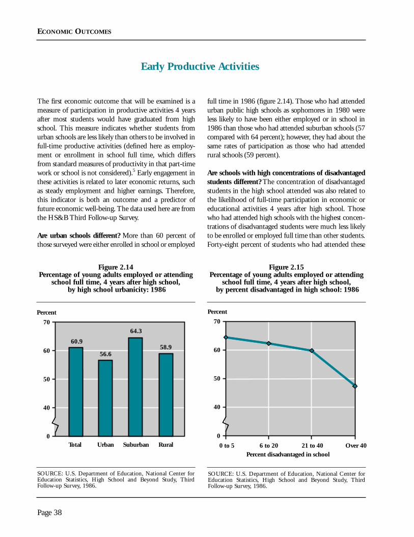
The first economic outcome that will be examined is ameasure of participation in productive activities 4 yearsafter most students would have graduated from highschool. This measure indicates whether students fromurban schools are less likely than others to be involved infull-time productive activities (defined here as employ-ment or enrollment in school full time, which differsfrom standard measures of productivity in that part-timework or school is not considered).5 Early engagement inthese activities is related to later economic returns, suchas steady employment and higher earnings. Therefore,this indicator is both an outcome and a predictor offuture economic well-being. The data used here are fromthe HS&B Third Follow-up Survey.
Are urban schools different? More than 60 percent ofthose surveyed were either enrolled in school or employed
full time in 1986 (figure 2.14). Those who had attendedurban public high schools as sophomores in 1980 wereless likely to have been either employed or in school in1986 than those who had attended suburban schools (57compared with 64 percent); however, they had about thesame rates of participation as those who had attendedrural schools (59 percent).
Are schools with high concentrations of disadvantagedstudents different? The concentration of disadvantagedstudents in the high school attended was also related tothe likelihood of full-time participation in economic oreducational activities 4 years after high school. Thosewho had attended high schools with the highest concen-trations of disadvantaged students were much less likelyto be enrolled or employed full time than other students.Forty-eight percent of students who had attended these
Page 38
ECONOMIC OUTCOMES
Early Productive Activities
Percent
Total Urban Suburban Rural0
40
50
60
7064.3
56.6
60.958.9
Percent disadvantaged in school0 to 5 6 to 20 21 to 40 Over 40
0
Percent
40
50
60
70
Figure 2.14Percentage of young adults employed or attending
school full time, 4 years after high school,by high school urbanicity: 1986
Figure 2.15Percentage of young adults employed or attending
school full time, 4 years after high school,by percent disadvantaged in high school: 1986
SOURCE: U.S. Department of Education, National Center forEducation Statistics, High School and Beyond Study, ThirdFollow-up Survey, 1986.
SOURCE: U.S. Department of Education, National Center forEducation Statistics, High School and Beyond Study, ThirdFollow-up Survey, 1986.

schools were engaged in full-time economic or educa-tional activities, compared with 60 to 64 percent ofstudents in other schools (figure 2.15).
Are urban schools different after accounting for dif-ferences in the concentration of disadvantagedstudents in the school? The difference between urbanand suburban students’ rates of participation in full-time economic or educational activities remains whenthe higher concentration of disadvantaged students inurban schools is taken into account. Therefore, anurban school location is related to this outcome inde-pendent of the higher concentration of disadvantagedstudents found in urban schools.
Were students from urban high schools with the high-est concentrations of disadvantaged students less likely
than predicted to be employed or enrolled in school fulltime 4 years after high school? Less than half of studentswho had attended an urban high school with the highestconcentration of disadvantaged students were employedor enrolled in school full time 4 years later (figure 2.16).However, this level of activity could be predicted from thecombined effects of urbanicity and high poverty concen-tration. These students were about as active as those whohad attended schools in suburban or rural areas with sim-ilarly disadvantaged populations.
Page 39
ECONOMIC OUTCOMES
Figure 2.16Percentage of young adults employed or attending school full time, 4 years after high school,
by high school urbanicity and percent disadvantaged in high school: 1986
Percent
0 to 5 6 to 20 21 to 40 Over 40
Suburban
UrbanRural
0
40
50
60
70
Percent disadvantaged in school
SOURCE: U.S. Department of Education, National Center for Education Statistics, High School and Beyond Study, Third Follow-upSurvey, 1986.
5“Employment” is defined as working for pay full time or on activeduty in the armed forces and not enrolled in college full time. Anadditional 10 percent of this group were employed part time,enrolled in school part time, or both, but these activities have beenexcluded from consideration. Expanding the analysis to includethese activities produces similar results as for full-time employmentor enrollment.

While the previous section examined productive activ-ities 4 years after a student typically leaves high school,this section examines the productive activities of youngadults after they have established patterns of activitythat are more reflective of the ones they will have dur-ing their prime working years. The measure ofparticipation in productive activities used here is thepercentage of young adults ages 25–32 who wereemployed or attending school full time in 1990, 7 to15 years after they typically would have finished highschool. In 1990, these young adults were asked whetherthey were engaged in productive economic or educa-tional activities full time. The NLSY is the source ofdata for this and the remaining economic indicators inthis chapter. The urbanicity and proportion of disad-vantaged students of the schools these young adultsattended have been identified.
Are urban schools different? In 1990, 84 percent ofyoung adults ages 25–32 were working at a job orenrolled in school full time. Young adults who hadattended urban public schools were less likely to beemployed or attending school (82 percent) than theircounterparts who had attended suburban schools (86percent); however, they were just as likely to be engagedin these activities as former rural students (82 percent)(figure 2.17).
Are schools with high concentrations of disadvan-taged students different? Young adults were generallyless likely to be engaged in productive activities if theyhad attended high schools with higher concentrationsof disadvantaged students. Seventy-six percent ofyoung adults who had attended high schools with thehighest concentration of disadvantaged students were
Page 40
ECONOMIC OUTCOMES
Later Productive Activities
Percent
Total Urban Suburban Rural0
70
75
80
85
95
86.4
82.384.2
81.5
90
Percent
0
70
75
80
85
95
90
Percent disadvantaged in school0 to 5 6 to 20 21 to 40 Over 40
Figure 2.17Percentage of young adults employed
or attending school full time, by high school urbanicity: 1990
Figure 2.18Percentage of young adults employed
or attending school full time, by percent disadvantaged in high school: 1990
SOURCE: U.S. Department of Labor, National LongitudinalSurvey of Youth, 1990.
SOURCE: U.S. Department of Labor, National LongitudinalSurvey of Youth, 1990.
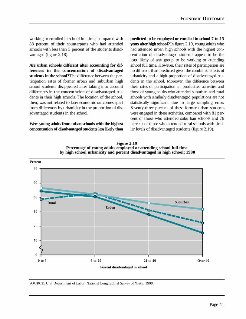
working or enrolled in school full time, compared with88 percent of their counterparts who had attendedschools with less than 5 percent of the students disad-vantaged (figure 2.18).
Are urban schools different after accounting for dif-ferences in the concentration of disadvantagedstudents in the school? The difference between the par-ticipation rates of former urban and suburban highschool students disappeared after taking into accountdifferences in the concentration of disadvantaged stu-dents in their high schools. The location of the school,then, was not related to later economic outcomes apartfrom differences by urbanicity in the proportion of dis-advantaged students in the school.
Were young adults from urban schools with the highestconcentration of disadvantaged students less likely than
predicted to be employed or enrolled in school 7 to 15years after high school? In figure 2.19, young adults whohad attended urban high schools with the highest con-centration of disadvantaged students appear to be theleast likely of any group to be working or attendingschool full time. However, their rates of participation areno different than predicted given the combined effects ofurbanicity and a high proportion of disadvantaged stu-dents in the school. Moreover, the difference betweentheir rates of participation in productive activities andthose of young adults who attended suburban and ruralschools with similarly disadvantaged populations are notstatistically significant due to large sampling error.Seventy-three percent of these former urban studentswere engaged in these activities, compared with 81 per-cent of those who attended suburban schools and 76percent of those who attended rural schools with simi-lar levels of disadvantaged students (figure 2.19).
Page 41
ECONOMIC OUTCOMES
Figure 2.19Percentage of young adults employed or attending school full time
by high school urbanicity and percent disadvantaged in high school: 1990
Percent
0 to 5 6 to 20 21 to 40 Over 40
Suburban
UrbanRural
0
75
85
90
95
Percent disadvantaged in school
80
70
SOURCE: U.S. Department of Labor, National Longitudinal Survey of Youth, 1990.

The unemployment rate indicates the portion of thelabor force that wish to be employed but are unable tofind work.6 The period during which the youth followedby the NLSY came of age and entered the labor market—the late 1970s through the 1980s—coincided with aperiod of higher overall unemployment, which dispro-portionately affected young, less educated, and minoritypopulations (Freeman 1991). This section will examinethe unemployment rates of young adults, ages 25–32,according to the urbanicity of the high school theyattended in the late 1970s and early 1980s, rather thantheir place of residence at the time of the follow-up sur-vey in 1990. Although the unemployment rates reportedin 1990 were affected by the job markets in places wherethe young adults were residing in 1990, it was not possi-ble to account for this effect in the following analysis.
Are urban schools different? In 1990, about 4 percentof young adults ages 25–32 were unemployed overall.But young adults who had attended public high schools
in urban areas had an average unemployment rate ofclose to 6 percent, while those from suburban and ruralschools had lower average unemployment rates of about3 and 4 percent, respectively (figure 2.20).
7
Are schools with high concentrations of disadvan-taged students different? The unemployment rates ofyoung adults generally increase with the proportion ofdisadvantaged students in the high school they attend.Young adults who had attended the schools with thehighest concentrations of disadvantaged students wereat least twice as likely to be unemployed as those fromschools with lower levels of disadvantaged students(almost 8 percent unemployed compared with 2 to 4percent from other schools) (figure 2.21).
Are urban schools different after accounting for dif-ferences in the concentration of disadvantagedstudents in the school? The urbanicity of the highschool attended continues to be related to the unem-
Page 42
ECONOMIC OUTCOMES
Unemployment
Percent
Total Urban Suburban Rural0
2
6
10
12
4
8
2.6
5.8
3.6 4.0
Percent disadvantaged in school0 to 5 6 to 20 21 to 40 Over 40
0
Percent
2
8
10
12
4
6
Figure 2.20Percentage of young adults unemployed,
by high school urbanicity: 1990
Figure 2.21Percentage of young adults unemployed,
by percent disadvantaged in high school: 1990
SOURCE: U.S. Department of Labor, National LongitudinalSurvey of Youth, 1990.
SOURCE: U.S. Department of Labor, National LongitudinalSurvey of Youth, 1990.

ployment rates of young adults, even when differencesby location in the proportion of disadvantaged studentsin the high school are considered. Young adults whohad attended urban schools would still have higherunemployment rates, even if their schools had the sameproportion of disadvantaged students as schools inother areas.
Were young adults from urban schools with thehighest concentration of disadvantaged studentsmore likely than predicted to be unemployed 7 to15 years after high school? Young adults who hadattended a high school located in an urban area withthe highest levels of disadvantaged students had anaverage unemployment rate of 11 percent, which wasmore than twice the rate (5 percent) for those whowent to similar schools in suburban areas (figure2.22). The difference between the unemploymentrates of those who had attended schools in urban and
rural areas with similarly high proportions of disad-vantaged students appears large in the figure;however, it is not statistically significant. Althoughthe urban unemployment rate of 11 percent is high,it is no higher than predicted from the combinationof the unemployment rates observed separately foryoung adults from all urban schools and from allschools with high concentrations of disadvantagedstudents. There is no evidence to suggest that therewas any additional unexplained unemployment foryoung adults who attended these schools that wasrelated to the combination of the school’s urban set-ting and highly disadvantaged population.
Page 43
ECONOMIC OUTCOMES
6“Unemployed” is defined as looking for work or on temporarylayoff and not enrolled in school full time.
7The difference between urban and rural here is significant at the90 percent confidence interval, rather than at the 95 percent con-fidence interval.
Figure 2.22Percentage of young adults unemployed,
by high school urbanicity and percent disadvantaged in high school: 1990
Percent
0 to 5 6 to 20 21 to 40 Over 40
Suburban
UrbanRural
0
2
8
10
12
Percent disadvantaged in school
4
6
SOURCE: U.S. Department of Labor, National Longitudinal Survey of Youth, 1990.

The average real earnings of young adults, in general,and of high school dropouts, in particular, declinedbetween 1979 and 1988. This combined with higherlevels of unemployment, as mentioned previously,drove many young adults in their prime into povertyby 1991 (Panel on High-Risk Youth 1993). Overalllevels of poverty are affected by broad economic anddemographic trends, but certain segments of thepopulation are at higher risk for living in povertythan others.8 Using data from the NLSY, this sectionaddresses whether young adults 25–32 who attendedpublic high school in urban areas in the late 1970sand early 1980s were more likely to be living inpoverty in 1990, when they were in their prime yearsof life, than those who attended suburban or ruralhigh schools.
Are urban schools different? In 1990, 8 percent ofyoung adults 25–32 were living below the poverty line.Young adults who had attended urban public highschools were much more likely to be living in poverty(15 percent) than their counterparts who had attendedsuburban or rural high schools (6 and 9 percent,respectively) (figure 2.23).
Are schools with high concentrations of disadvan-taged students in the school different? Young adultswho had attended a high school with the highest con-centrations of disadvantaged students were three timesas likely to be living in poverty in 1990 (15 percent) astheir counterparts who had attended schools with thelowest concentration of disadvantaged students (5 per-cent) (figure 2.24).
Page 44
ECONOMIC OUTCOMES
Poverty Status
Percent
Total Urban Suburban Rural0
5
15
25
30
10
20
6.0
14.5
8.3 8.6
Percent disadvantaged in school0 to 5 6 to 20 21 to 40 Over 40
0
Percent
30
5
15
25
10
20
Figure 2.23Percentage of young adults living in poverty,
by high school urbanicity: 1990
Figure 2.24Percentage of young adults living in poverty,
by percent disadvantaged in high school: 1990
SOURCE: U.S. Department of Labor, National LongitudinalSurvey of Youth, 1990.
SOURCE: U.S. Department of Labor, National LongitudinalSurvey of Youth, 1990.

Are urban schools different after accounting fordifferences in the concentration of disadvantagedstudents in the school? Students who had attendedurban high schools were more likely to be living inpoverty later in life, even after the proportion of dis-advantaged students in their schools was taken intoaccount.
Were young adults from urban schools with the high-est concentration of disadvantaged students morelikely to be living in poverty 7 to 15 years after highschool than predicted? One out of four young adultswho had attended urban high schools with the highestproportions of disadvantaged students were livingbelow the poverty line in 1990. This contrasts with one
out of seven young adults who had attended similarschools in suburban locations, and one out of 10 fromrural locations (figure 2.25). One out of 27 studentsfrom suburban schools with the lowest level of disad-vantaged students ended up living in poverty. Thepoverty rate in the prime of life for students from urbanschools with high concentrations of disadvantaged stu-dents, though higher than other schools, is no higherthan predicted from the additive effect of high con-centrations of disadvantaged students and the urbanlocation of the high schools.
Page 45
ECONOMIC OUTCOMES
8In addition to employment and earnings, family size and the ageof the householder (in one- and two-person families) has an impacton the calculation of poverty status.
Figure 2.25Percentage of young adults living in poverty,
by high school urbanicity and percent disadvantaged in high school: 1990
Percent
0 to 5 6 to 20 21 to 40 Over 40
Suburban
Urban
Rural
0
5
20
25
30
Percent disadvantaged in school
10
15
SOURCE: U.S. Department of Labor, National Longitudinal Survey of Youth, 1990.


This chapter examines the influences and activities thataffect students’ performance in school but that liebeyond the school’s control. Although the chapter pri-marily focuses on family-related backgroundcharacteristics, such as parental employment, it alsoaddresses students’ extracurricular activities and part-time work. Clearly, the choices students make abouthow they spend their time outside of school may affecttheir performance in school as well as their futureemployment.
The background characteristics of students that arediscussed in this chapter were selected on the basis ofprevious research documenting their relationship tostudents’ educational outcomes. Since Coleman’slandmark study, Equality of Educational Opportunity(Coleman et al. 1966), numerous studies have foundthat family and socioeconomic characteristics areclosely tied to a student’s chances for academic suc-cess. For example, in a study of young adult literacy,parents’ education was found to be significantly relat-ed to literacy behavior and type and amount ofeducation young adults eventually achieve (Kirschand Jungeblut 1986). Many believe that students inurban schools are less likely than students in otherschools to have the family and economicresources that have been shown to predict acade-mic success.
Further, it has been hypothesized that students whoparticipate in school extracurricular activities are morelikely to become engaged in school (Braddock 1991;Newmann 1992; Finn 1993). Research findings seemto show that students who participate in extracurricu-lar activities have better grades, spend more time onhomework, and have higher school aspirations.
While students’ participation in extracurricular activ-ities seems to positively affect their schoolperformance, their working at a job during the
school year may have mixed effects. On the positiveside, working may increase the student’s sense ofresponsibility, and early exposure to work experiencesmay promote future labor market success (Mangum1988). On the negative side, however, student laborforce participation has also been hypothesized toadversely affect student school engagement and out-comes (Newmann 1992).
Although this chapter examines each student back-ground characteristic separately, the familycharacteristics that are discussed tend to be interre-lated and linked to a student’s likelihood of living inpoverty. For example, a child from a one-parent fam-ily is more likely to be living in poverty, as is a childwhose parent has lower educational attainment(Committee on Ways and Means, U.S. House ofRepresentatives 1985). Similarly, because householdswith lower income levels are more mobile, the chil-dren in those households would be more likely tochange schools. While this chapter discusses theseand other selected family background characteristics,chapter 1 provides more descriptive informationabout the socioeconomic status of students accordingto the type of school they attend and its location.
The data in this chapter are drawn from the base yearand first follow-up of a longitudinal survey that beganwith a cohort of 8th-grade students, the NationalEducation Longitudinal Study of 1988 (NELS:88). Inaddition to information on students, NELS:88includes information gathered directly from students’parents. Parents tend to be a more reliable source thanthe students themselves for information about parentaland other family background characteristics.
Like the analysis in chapter 2, in this chapter studentsare grouped according to the urbanicity and the level ofpoverty concentration in the school they attended. Thedata for each measure are subjected to a series of statis-
Page 47
Chapter 3
Student Background Characteristicsand Afterschool Activities

tical tests (using analysis of variance techniques) todetermine:
1) If urban students, in general, have fewer familyand economic resources and lower participationrates (in extracurricular activities or in the laborforce) than suburban or rural students;
2) If students from schools with higher povertyconcentrations have fewer background resourcesand different participation rates than studentsfrom schools with lower poverty concentrations;
3) If the background resources and participationrates of students from urban public schoolswould still differ from those of students fromrural and suburban public schools if the level ofpoverty concentration poverty of their schoolswere held constant; and
4) If students in the urban schools with the highestpoverty concentrations have fewer backgroundresources and are less likely to participate inafterschool activities and less likely to be workingpart time than their suburban and rural counter-parts and if so, were their family backgroundsand activities different than predicted.
Chart 3.1 lists the indicators that were used in this chap-ter and summarizes the findings for those indicators. Thechart may be used as a reference, because the four basicquestions addressed in this report are answered briefly foreach characteristic discussed in this chapter.
This chapter is divided into two sections: student back-ground characteristics and afterschool activities. The firstsection addresses whether a student lives with two par-ents, parental employment, whether a parent completedcollege, school mobility, parental expectations for thechild to complete college, and parent and child conversa-tions about school. The second section, on afterschoolactivities, focuses on sports-related activities offered bythe schools attended by 8th graders, students’ partici-pation rates in these activities, and studentemployment.
Summary of This Chapter’s Findings
Urban students and students who attend public schoolswith high poverty concentrations are, in general, morelikely to have fewer economic and human resources—they are less likely to have two parents in the householdand their parents have lower educational attainment.They are also likely to participate in extracurricularactivities at lower rates. Even after accounting forschool poverty concentration, the following patternsemerged for urban students:
• They were less likely to live in two-parent fami-lies;
• Those who lived in a two-parent family were lesslikely than suburban students to have a parentemployed full time;
• They were more likely to have changed schoolsmore than once; and
• They were less likely to participate in school-sponsored extracurricular sports activities.
For two of the indicators of student background andafterschool activities that were examined, students froman urban school with the highest poverty concentrationexperienced a higher level of risk than those in highpoverty schools elsewhere.9 These indicators for whichurban high poverty students were at higher risk thanhigh poverty students from other locations were:
• They were less likely to live in a two-parentfamily; and
• They were more likely to change schools morethan once.
Of the remaining eight indicators, a similar level of riskwas found among students in high poverty schools insuburban and rural locations.
For all of the indicators that were examined in this sec-tion, students attending urban high poverty public
Page 48

schools fared just as well as would be predicted from thecombination of urban and high poverty school charac-teristics. That is, the students’ backgroundcharacteristics and afterschool activities could be pre-dicted from the combined effects of an urban and a highpoverty setting. There was no evidence that they wereassociated with an interaction, or compounding effect,of an urban setting and high poverty.
Page 49
9The term risk is used because research findings indicate that theseparticular characteristics seem to be related to a greater likelihood ofpoor educational outcomes. For example, children living with onlyone parent and those whose parents are not employed do not per-form as well in school as those living in two-parent households orthose having at least one parent who is employed.
Are Urban Are High Are Urban Are Urban HighSchools Poverty Schools Schools Poverty SchoolsDifferent? Different? Different after Different from
Accounting for Other HighPoverty Poverty Schools?Concentration?
Are Urban HighPoverty SchoolsDifferent than
INDICATOR Predicted?
I. STUDENT BACKGROUND CHARACTERISTICS
Living in Yes, Yes, Yes, Yes,Two-Parent urban lower than high poverty lower urban lower than lower thanFamily suburban and than all others others other high poverty
ruralNo differentthan predicted
Single-Parent Yes, Yes, No, No,Family, urban lower than high poverty lower urban same same as otherParent Works suburban, but than all others as others high poverty
same as ruralNo differentthan predicted
Two-Parent Yes, Yes, Yes, No,Family, at urban lower than high poverty lower urban lower than same as otherLeast One suburban, but than all others suburban, high povertyParent Works same as rural same as rural
No differentthan predicted
Parent Yes, Yes, Yes, No,Completed urban lower than high poverty lower urban same as same as otherCollege suburban, than all others suburban, high poverty
same as rural higher thanrural No different
than predicted
CHART 3.1—SUMMARY OF RESULTS:STUDENT BACKGROUND CHARACTERISTICS AND AFTERSCHOOL ACTIVITIES

Page 50
Are Urban Are High Are Urban Are Urban HighSchools Poverty Schools Schools Poverty SchoolsDifferent? Different? Different after Different from
Accounting for Other HighPoverty Poverty Schools?Concentration?
Are Urban HighPoverty SchoolsDifferent than
INDICATOR Predicted?
Student Changed Yes, Yes, Yes, Yes,Schools More urban higher than high poverty higher urban higher than higher thanThan Once suburban and than most others others other high
rural poverty
No differentthan predicted
Parent Expects Yes, Yes, Yes, No,Student to urban lower than high poverty lower urban same as same as otherComplete suburban, than most others suburban, high povertyCollege higher than higher than
rural rural No differentthan predicted
Parent Talks Yes, Yes, No, No,with Student urban lower than high poverty lower urban same as same as otherabout School suburban and than all others high poverty
rural othersNo differentthan predicted
II. AFTERSCHOOL ACTIVITIES
School Sports Yes, Yes, Yes, Yes,Offerings urban lower than high poverty lower urban higher than higher than
suburban, higher than most rural, same as rural high poverty,than rural others suburban same as suburban
high poverty
No differentthan predicted
Student Sports Yes, Yes, Yes, No,Participation urban lower than high poverty lower urban lower than same as
suburban and than all others others other high povertyrural
No differentthan predicted
Student No, Yes, No, No,Labor Force urban same as high poverty lower urban same as same asParticipation suburban and than most others others other high poverty
rural othersNo differentthan predicted

Family support and resources have been shown to sig-nificantly affect student’s school progress. Thus, it isimportant to determine whether urban students havesimilar levels of family and socioeconomic resources asdo students in suburban and rural schools.
Findings
• On all but one of the background indicators,student labor force participation, urban publicschool students fared less well than students whoattended suburban public schools. However, onmore than half of the indicators examined in thischapter, urban students fared as well as or betterthan rural students. Those indicators on whichurban students fared less well than rural studentswere school mobility, talks with parents aboutschool, sports participation, and family livingarrangements.
• There appears to be a strong relationship betweenbackground characteristics that have been shownto put students at greater risk and the level of
poverty concentration of the school that theyattend. Among all the indicators reviewed, stu-dents attending high poverty schools generallyfared less well than students attending schoolswith lower poverty concentrations.
• Even after accounting for the level of poverty inthe schools, students who attended urbanschools had a greater level of risk than those whoattended suburban and rural schools in the areasof family structure and school mobility.10 Amongthe remaining indicators, their level of risk wasless than or equal to that of students attendingother schools.
• Compared with students in high poverty schoolsin other locations, students who attended urbanhigh poverty schools were less likely to live in atwo-parent family and were more likely to havechanged schools more than once.
Page 51
Student Background Characteristics
10Chapter 1 contains a broad descriptive discussion of studentcharacteristics by urbanicity.

STUDENT BACKGROUND CHARACTERISTICS
Whether a child lives with one parent or two has beenfound to be related to a child’s success in school(Mulkey et al. 1992). All other things being equal,with only one parent in the household, that parent islikely to have less time to spend with the child thanparents in two-parent households. Also, in one-parenthouseholds, household income is generally lower thanit is in two-parent households, which may producemore economic stress in the household and, in turn,affect a student’s school performance.
Are urban schools different? In 1988, about three-quarters of all 8th graders lived in households inwhich two parents were present (figure 3.1).11
However, 8th-grade students in suburban or ruralschools were more likely than urban students to beliving with two parents. Approximately 80 percent of
suburban and rural students lived with two parents,compared with only 68 percent of urban students.
Are high poverty schools different? Students inschools with higher concentrations of poverty wereless likely to be living with two parents than studentsin schools with lower levels of poverty (figure 3.2).Eighty-five percent of 8th graders in schools with thelowest concentration of poverty lived with two par-ents, while 71 percent of students in schools withhigh poverty concentrations did so.
Are urban schools different after accounting forpoverty concentration? While chapter 1 has shownthat urbanicity and poverty concentration are highlyrelated, students in urban schools were less likely thanother students to be living in two-parent households
Page 52
Two-Parent Families
Percent
Total Urban Suburban Rural0
50
60
70
80
90
80.7 79.677.5
67.7
Percent
School poverty concentration(percent)
0 to 5 6 to 20 21 to 40 Over 400
50
60
70
80
90
Figure 3.1Percentage of 8th-grade students living in a
two-parent family, by urbanicity: 1988
Figure 3.2Percentage of 8th-grade students living in a two-parent
family, by school poverty concentration: 1988
SOURCE: U.S. Department of Education, National Center forEducation Statistics, National Education Longitudinal Study of1988, Base Year Survey.
SOURCE: U.S. Department of Education, National Center forEducation Statistics, National Education Longitudinal Study of1988, Base Year Survey.
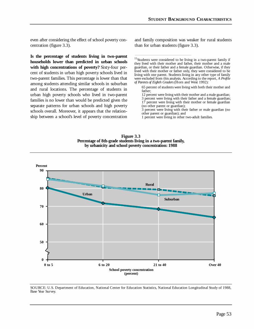
STUDENT BACKGROUND CHARACTERISTICS
even after considering the effect of school poverty con-centration (figure 3.3).
Is the percentage of students living in two-parenthouseholds lower than predicted in urban schoolswith high concentrations of poverty? Sixty-four per-cent of students in urban high poverty schools lived intwo-parent families. This percentage is lower than thatamong students attending similar schools in suburbanand rural locations. The percentage of students inurban high poverty schools who lived in two-parentfamilies is no lower than would be predicted given theseparate patterns for urban schools and high povertyschools overall. Moreover, it appears that the relation-ship between a school’s level of poverty concentration
and family composition was weaker for rural studentsthan for urban students (figure 3.3).
Page 53
11Students were considered to be living in a two-parent family ifthey lived with their mother and father, their mother and a maleguardian, or their father and a female guardian. Otherwise, if theylived with their mother or father only, they were considered to beliving with one parent. Students living in any other type of familywere excluded from this analysis. According to the report, A Profileof Parents of Eighth Graders (Horn and West 1992):
65 percent of students were living with both their mother andfather;12 percent were living with their mother and a male guardian; 3 percent were living with their father and a female guardian; 17 percent were living with their mother or female guardian(no other parent or guardian);3 percent were living with their father or male guardian (noother parent or guardian); and1 percent were living in other two-adult families.
Figure 3.3Percentage of 8th-grade students living in a two-parent family,
by urbanicity and school poverty concentration: 1988
Percent
School poverty concentration(percent)
0 to 5 6 to 20 21 to 40 Over 40
SuburbanUrban
Rural
0
50
60
70
80
90
SOURCE: U.S. Department of Education, National Center for Education Statistics, National Education Longitudinal Study of 1988,Base Year Survey.

There is evidence that parental employment influencesfamily social and economic well-being in both negativeand positive ways. This is true for several reasons. Thenumber of earners in a family is related to the level offamily income (U.S. Bureau of the Census 1993). Inaddition, if the male parent is not employed it can placegreat stress upon the family and may lead to a greater riskof family marital disruption (Bianchi and McArthur1991). Thus parental employment can be seen as a pos-itive attribute for a student in that the student is morelikely to be living in a stable, more economically securesituation. Also, parents who are in the labor force mayserve as positive role models for their children.
However, parental employment can have a negativeimpact when their working hours leave little time tospend with children, which may be especially true infamilies where there is a single parent.
Using information from NELS:88, this analysis breaksout employment status separately for parents of 8thgraders when there is one parent in the household andwhen there are two.12 For students living with one par-ent, the category of interest is whether that parent isworking full time (contrasted to parents who are work-ing part time, who are unemployed, or who are not inthe labor force), because the primary interest in this
Page 54
STUDENT BACKGROUND CHARACTERISTICS
Parental Employment
Total Urban Suburban Rural
71.3
64.6
59.4
Percent
65.4
0
50
75
80
60
70
55
65
Percent
0
50
75
80
60
70
55
65
School poverty concentration(percent)
0 to 5 6 to 20 21 to 40 Over 40
Figure 3.4Percentage of 8th-grade students living in
a one-parent family with parent working full time, by urbanicity: 1988
Figure 3.5Percentage of 8th-grade students living in
a one-parent family with parent working full time, by school poverty concentration: 1988
SOURCE: U.S. Department of Education, National Center forEducation Statistics, National Education Longitudinal Study of1988, Base Year Survey.
SOURCE: U.S. Department of Education, National Center forEducation Statistics, National Education Longitudinal Study of1988, Base Year Survey.
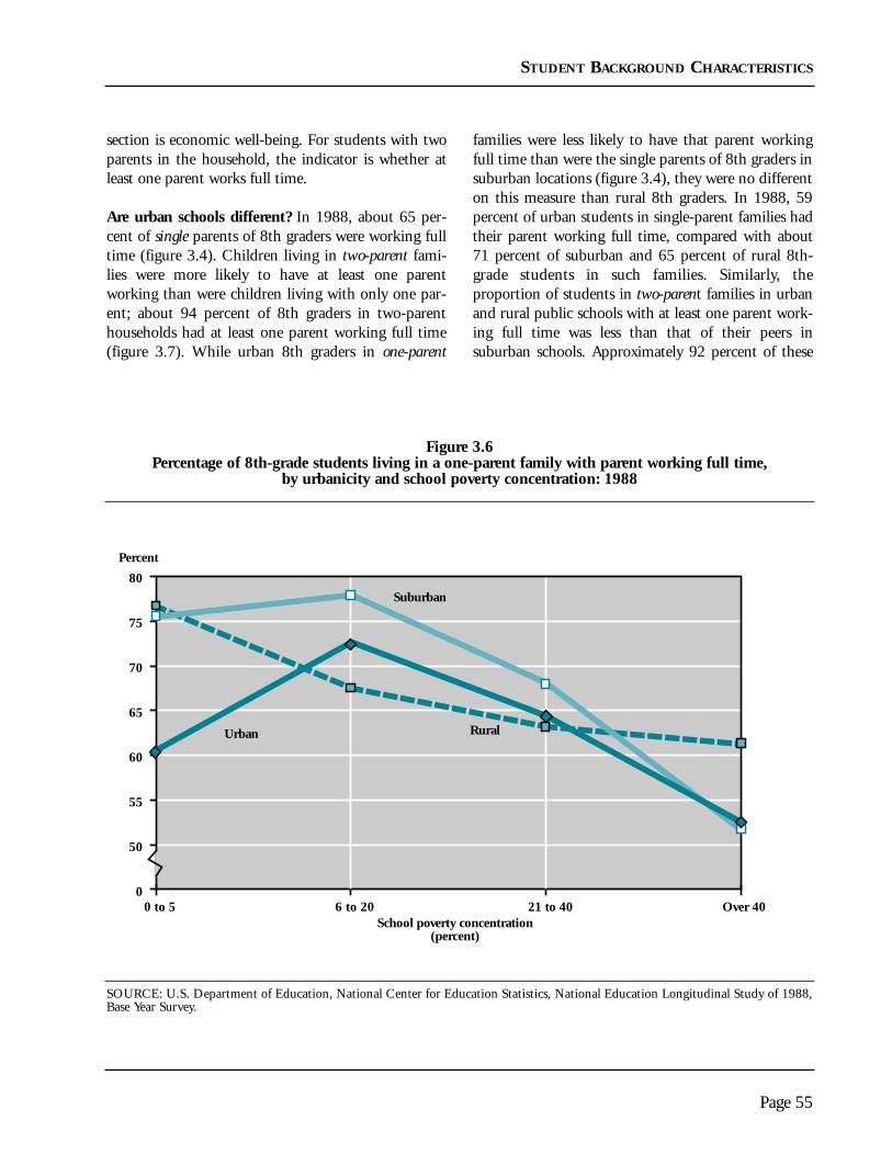
STUDENT BACKGROUND CHARACTERISTICS
section is economic well-being. For students with twoparents in the household, the indicator is whether atleast one parent works full time.
Are urban schools different? In 1988, about 65 per-cent of single parents of 8th graders were working fulltime (figure 3.4). Children living in two-parent fami-lies were more likely to have at least one parentworking than were children living with only one par-ent; about 94 percent of 8th graders in two-parenthouseholds had at least one parent working full time(figure 3.7). While urban 8th graders in one-parent
families were less likely to have that parent workingfull time than were the single parents of 8th graders insuburban locations (figure 3.4), they were no differenton this measure than rural 8th graders. In 1988, 59percent of urban students in single-parent families hadtheir parent working full time, compared with about71 percent of suburban and 65 percent of rural 8th-grade students in such families. Similarly, theproportion of students in two-parent families in urbanand rural public schools with at least one parent work-ing full time was less than that of their peers insuburban schools. Approximately 92 percent of these
Page 55
Figure 3.6Percentage of 8th-grade students living in a one-parent family with parent working full time,
by urbanicity and school poverty concentration: 1988
School poverty concentration(percent)
Percent
0 to 5 6 to 20 21 to 40 Over 40
Suburban
Urban Rural
0
50
75
80
60
70
55
65
SOURCE: U.S. Department of Education, National Center for Education Statistics, National Education Longitudinal Study of 1988,Base Year Survey.

urban and rural students had at least one parent working,while 95 percent of suburban students did so (figure 3.7).
Are high poverty schools different? Students living insingle-parent and two-parent families who attendedschools serving large proportions of disadvantaged stu-dents were less likely than other students to have theirparent working (figures 3.5 and 3.8). In the schoolswith the highest poverty concentrations, 55 percent ofstudents in one-parent families had a working parentcompared with over 74 percent of 8th graders in one-parent families from schools with the lowest povertyconcentration. Similarly, of students in two-parent fam-ilies in schools with the highest poverty concentrations,88 percent had at least one parent working full time,compared with 97 percent of students in schools withthe lowest poverty concentrations.
Are urban schools different after accounting forpoverty concentration? Urban students who lived withtwo parents were less likely to have a parent employedfull time even after accounting for differences in pover-ty concentration in each location (figure 3.9). Afteraccounting for poverty concentration, differences inparental employment status between urban studentswho lived with one parent and their suburban and ruralcounterparts were not significant (figure 3.6).
Is the percentage of students with parents working fulltime lower than predicted in urban schools with highconcentrations of poverty? Among students in urbanhigh poverty schools, 53 percent of those living with oneparent and 88 percent of those living with two parentshad a parent working full time. These students were justas likely as comparable students attending high poverty
Page 56
STUDENT BACKGROUND CHARACTERISTICS
95.4
91.791.7
Percent
0
80
95
100
85
90
93.5
Total Urban Suburban RuralSchool poverty concentration
(percent)
Percent
0
80
95
100
85
90
0 to 5 6 to 20 21 to 40 Over 40
Figure 3.7Percentage of 8th-grade students living in
a two-parent family with at least one parent working full time, by urbanicity: 1988
Figure 3.8Percentage of 8th-grade students living in a two-parent family with at least one parent working
full time, by school poverty concentration: 1988
SOURCE: U.S. Department of Education, National Center forEducation Statistics, National Education Longitudinal Study of1988, Base Year Survey.
SOURCE: U.S. Department of Education, National Center forEducation Statistics, National Education Longitudinal Study of1988, Base Year Survey.

STUDENT BACKGROUND CHARACTERISTICS
schools in suburban and rural locations to have a parentworking full time. (The difference in figure 3.6 is notstatistically significant.) The percentage of students,whether living in one- or two-parent families, with a par-ent working full time was no lower than predicted inurban schools with high concentrations of poverty.
Figure 3.9Percentage of 8th-grade students living in a two-parent family with at least one parent working
full time, by urbanicity and school poverty concentration: 1988
School poverty concentration(percent)
Percent
Suburban
Urban
Rural
0
80
90
95
100
85
0 to 5 6 to 20 21 to 40 Over 40
SOURCE: U.S. Department of Education, National Center for Education Statistics, National Education Longitudinal Study of 1988,Base Year Survey.
12Information about “parental” labor force status was reported bythe parent or guardian who responded to the parent questionnaire.That person reported his/her labor force status as well as that of aspouse/partner if one was present in the household. Refer to foot-note 11 for more information about family composition.
Page 57

Page 58
STUDENT BACKGROUND CHARACTERISTICS
The association between parents’ educational level andtheir children’s potential academic success has been welldocumented. Children with more highly educated par-ents have higher educational achievement andattainment (Barro and Kolstad 1987; Kirsch andJungeblut 1986; Kaufman and Bradby 1991; Horn andWest 1992; McArthur 1993; Natriello et al. 1990).Further, parents with higher education also tend tohave higher expectations for their children’s education-al outcomes (Horn and West 1992). If at least oneparent has completed 4 or more years of college, house-hold income tends to be higher, with parents havinggreater access to economic resources to support a child(U.S. Bureau of the Census 1992).
The NELS:88 parent survey asked the parent orguardian who responded to report his or her own high-
est level of education. If that person had a partner orspouse in the household, that person’s educational levelwas also ascertained. In the analysis presented here, ifthere are two parent/guardians in the household, thehighest level of education reported for either parent isused. For the sake of economy, the “parent or guardian”will be referred to as the “parent.” (See footnote 11 fora description of family composition in the NELS:88base year survey.)
Are urban schools different? In 1988, about 24 percentof all 8th graders had at least one parent in the house-hold who had completed 4 years of college (figure3.10). Children in urban schools were less likely tohave a college-educated parent than were children insuburban schools. Twenty percent of urban childrenhad at least one parent who had completed 4 years of
Parents’ Educational Attainment
Total Urban Suburban Rural
Percent
0
10
20
30
40
50
29.5
18.620.4
23.7
Percent
School poverty concentration(percent)
0 to 5 6 to 20 21 to 40 Over 400
10
20
30
40
50
Figure 3.10Percentage of 8th-grade students with a parent in the household who had completed 4 years
of college, by urbanicity: 1988
Figure 3.11Percentage of 8th-grade students with a parent in the household who had completed 4 years ofcollege, by school poverty concentration: 1988
SOURCE: U.S. Department of Education, National Center forEducation Statistics, National Education Longitudinal Study of1988, Base Year Survey.
SOURCE: U.S. Department of Education, National Center forEducation Statistics, National Education Longitudinal Study of1988, Base Year Survey.

STUDENT BACKGROUND CHARACTERISTICS
college or more, compared with almost 30 percent ofsuburban 8th graders. However, urban students wereequally as likely to have a college-educated parent aswere rural students.
Are high poverty schools different? Children fromschools with the highest concentrations of poverty weremuch less likely to have at least one college-educatedparent than students in schools with lower levels ofschool poverty (figure 3.11). Eleven percent of childrenin high poverty schools had a parent who had complet-ed 4 years of college or more, compared with over 41percent of children from low poverty schools.
Are urban schools different after accounting forpoverty concentration? After the poverty concentra-
tion of the schools in each location was considered,urban and suburban students were equally likely tohave at least one parent who had completed 4 years ormore of college (figure 3.12). However, rural studentswere less likely than urban students to have at least onecollege-educated parent.
Is the percentage of students with a college-educatedparent lower than predicted in urban schools with highconcentrations of poverty? While 12 percent of studentsin urban high poverty schools had a college-educatedparent, these students were equally as likely as studentsin similar schools in suburban and rural locations to havesuch parents. The percentage of students with a college-educated parent was no lower than predicted in urbanschools with high concentrations of poverty.
Page 59
Figure 3.12Percentage of 8th-grade students with a parent in the household who had completed 4 years of college,
by urbanicity and school poverty concentration: 1988
School poverty concentration(percent)
0 to 5 6 to 20 21 to 40 Over 40
0
10
20
30
40
50Percent
Suburban
Urban
Rural
SOURCE: U.S. Department of Education, National Center for Education Statistics, National Education Longitudinal Study of 1988,Base Year Survey.

Previous research has linked student mobility (that is,changing schools) with students having increased acad-emic and disciplinary problems in school (Bianchi1993; Haveman, Wolfe, and Spaulding 1991; Straits1987; Long 1975).13 The negative impact of mobilityupon schooling can be explained by a number of fac-tors, for example, differences across schools or districtsin academic requirements. Another explanation couldbe that students who frequently change schools mayhave difficulty becoming attached to a new school,which might decrease their motivation to learn. A stu-dent’s likelihood of changing schools is also linked tothe likelihood of being victimized at school (Bastianand Taylor 1991). This section focuses on schoolmobility by identifying 8th-grade students whochanged schools two or more times since first grade forreasons other than a promotion to one grade or level or
a move from an elementary school building to a mid-dle school building in the same district.
Are urban schools different? Eighth graders attendingurban public schools in 1988 were more likely thanother 8th-grade students to have changed schools twoor more times since the first grade (figure 3.13). Almost46 percent of urban students had changed school thisoften, compared with only 34 percent of suburban and28 percent of rural students.
Are high poverty schools different? Students in schoolswith the highest concentrations of poverty had changedschools more often than students in schools with thelowest concentrations of poverty (figure 3.14). About38 percent of students in schools with the highest levelof school poverty concentration had changed schools
Page 60
STUDENT BACKGROUND CHARACTERISTICS
School Mobility
Percent
Total Urban Suburban Rural0
20
30
40
50
60
33.6
28.0
45.6
34.2
Percent
0 to 5 6 to 20 21 to 40 Over 400
20
30
40
50
60
School poverty concentration(percent)
Figure 3.13Percentage of 8th-grade students who have
changed schools more than once since first grade,by urbanicity: 1988
Figure 3.14Percentage of 8th-grade students who have
changed schools more than once since first grade,by school poverty concentration: 1988
SOURCE: U.S. Department of Education, National Center forEducation Statistics, National Education Longitudinal Study of1988, Base Year Survey.
SOURCE: U.S. Department of Education, National Center forEducation Statistics, National Education Longitudinal Study of1988, Base Year Survey.

STUDENT BACKGROUND CHARACTERISTICS
two or more times, compared with 31 percent of stu-dents in schools with the lowest concentration ofpoverty. There was no real difference between themobility rates of students in schools with highestpoverty and next to highest poverty concentrations.
Are urban schools different after accounting forpoverty concentration? Even after the school povertyconcentration in each location was considered, urbanstudents were still more likely than suburban or ruralstudents to have moved two or more times (figure3.15).
Is student mobility higher than predicted in urbanschools with high concentrations of poverty? Studentsin urban high poverty schools were more likely to have
changed schools two or more times than were studentsin similar suburban and rural schools. Forty-six percentof these students changed schools this often, comparedwith 37 percent of suburban and 29 percent of ruralstudents in similar schools. The difference in studentmobility between urban high poverty schools and otherschools was no greater than would be predicted given therates of student mobility for urban and high povertyschools taken separately. This suggests that the combina-tion of high poverty concentration and an urban settingdoes not add to the already higher risk for these studentsto change schools.
Page 61
Figure 3.15Percentage of 8th-grade students who have changed schools more than once since first grade,
by urbanicity and school poverty concentration: 1988
Suburban
Urban
Rural
0
School poverty concentration(percent)
Percent
20
30
40
50
60
0 to 5 6 to 20 21 to 40 Over 40
SOURCE: U.S. Department of Education, National Center for Education Statistics, National Education Longitudinal Study of 1988,Base Year Survey.
13It should be noted that the negative impact of school mobilityalso could be due in part to underlying problems such as familyinstability.

A student’s success in school is tied to parental expecta-tions for their child’s education. In many instances,parental expectations translate into prescriptions fortheir child’s behavior, which include rules about home-work and rules about maintaining a certain grade pointaverage, as well as expectations about how well theirchild will do in school and how much education thechild will eventually complete. Thus, at the same timethat parental expectations may influence the student’simmediate behavior, they may also affect the student’sself-concept and motivation to learn (Horn and West1992). For this analysis, the measure of parental expec-tations used is whether parents expect their 8th graderto complete 4 or more years of college, since collegecompletion directly affects labor market success. Aswith previous sections on parental labor force partici-
pation and their education, both parents and guardiansare included here and referred to simply as “parents.”(See footnote 11 for a discussion of family compositionin NELS:88.)
Are urban schools different? In 1988, the parents ofmost 8th graders held high expectations for their chil-dren’s education (figure 3.16). The parents of over halfthe children expected them to graduate from collegewith a 4-year degree.14 Parental expectations on averagewere higher for students in urban schools than for ruralstudents, but were lower than those for suburban stu-dents. Almost 56 percent of urban students had parentswho expected them to eventually receive a 4-yeardegree, compared with 49 percent of rural students and60 percent of suburban students.
Page 62
STUDENT BACKGROUND CHARACTERISTICS
Parents’ Expectations for Their Child’s Education
Percent
Total Urban Suburban Rural0
40
50
60
70
80
60.2
49.0
55.755.3
Percent
School poverty concentration(percent)
0 to 5 6 to 20 21 to 40 Over 400
40
50
60
70
80
Figure 3.16Percentage of 8th-grade students whose parents
expect them to complete 4 years of college,by urbanicity: 1988
Figure 3.17Percentage of 8th-grade students whose parents
expect them to complete 4 years of college,by school poverty concentration: 1988
SOURCE: U.S. Department of Education, National Center forEducation Statistics, National Education Longitudinal Study of1988, Base Year Survey.
SOURCE: U.S. Department of Education, National Center forEducation Statistics, National Education Longitudinal Study of1988, Base Year Survey.

STUDENT BACKGROUND CHARACTERISTICS
Are high poverty schools different? Parents of childrenin schools with relatively large concentrations of poorchildren were far less likely to expect their children tofinish college than parents of children in other schools(figure 3.17). The parents of almost two-thirds of the8th graders in low poverty schools expected them tofinish a 4-year college program, compared with 49 per-cent of the parents of 8th graders in high povertyschools.
Are urban schools different after accounting forpoverty concentration? Only the difference betweenurban and rural schools remained significant afteraccounting for poverty concentration. However, therewere no significant differences between urban and sub-urban schools after accounting for povertyconcentration. The educational expectations of the par-ents of urban and suburban students declined similarly
with increasing school poverty (figure 3.18). But forrural students, the parents’ expectations varied littleacross the categories of concentrations of poverty:about 50 percent of all rural students had parents whothought their child would complete a 4-year collegeprogram, regardless of poverty concentration level.
Are parental expectations lower than predicted inurban schools with high concentrations of poverty?The parental expectations of students in urban highpoverty concentration schools were no lower thanwould be predicted. In fact, regardless of urbanicity, theparents of about half of students in high povertyschools expected them to complete 4 years of college.
Page 63
Figure 3.18Percentage of 8th-grade students whose parents expect them to complete 4 years of college,
by urbanicity and school poverty concentration: 1988
School poverty concentration(percent)
0 to 5 6 to 20 21 to 40 Over 40
0
40
50
60
70
80Percent
Suburban
Urban
Rural
SOURCE: U.S. Department of Education, National Center for Education Statistics, National Education Longitudinal Study of 1988,Base Year Survey.
14Given the fact that in 1990 less than a third of all 25- to 32-year-olds held a bachelor's degree or higher, these expectations may beunrealistically high. See figure 2.11 in chapter 2 of this report.

Parent involvement in their child’s education may takemany forms. These include participation inparent/teacher organizations, volunteering at theschool, contacting the school about the child’s progress,monitoring homework, talking with their child aboutwhat they do in school, and talking about future edu-cation plans.
This section addresses one such aspect of parentinvolvement, the frequency with which the parents talkwith their 8th-grade students about school. Theassumption made is that talking with the child aboutschool on a regular basis shows the student that the par-ent cares about school issues and keeps the parentinformed about school activities.
Are urban schools different? In 1988, the parents ofmore than three out of four 8th graders talked withtheir child about school (figure 3.19), but the parentsof 22 percent of public school students rarely did so.15
Parents of urban students were less likely to regularlytalk to their child than were parents of rural or subur-ban students. The differences by urbanicity, whilesmall, were significant: the parents of about one-fourthof urban students rarely talked to their child aboutschool, compared with the parents of about 23 percentof rural students and one-fifth of suburban students.
Are high poverty schools different? Parents of studentsin schools with high concentrations of poverty were lesslikely than parents of students in other schools to have
Page 64
STUDENT BACKGROUND CHARACTERISTICS
Parent and Child Conversations About School
Percent
0
10
20
30
40
19.622.5
24.921.7
Total Urban Suburban Rural
Percent
School poverty concentration(percent)
0 to 5 6 to 20 21 to 40 Over 400
10
20
30
40
Figure 3.19Percentage of 8th-grade students whose parents
rarely talk to them about school,by urbanicity: 1988
Figure 3.20Percentage of 8th-grade students whose parents
rarely talk to them about school,by school poverty concentration: 1988
SOURCE: U.S. Department of Education, National Center forEducation Statistics, National Education Longitudinal Study of1988, Base Year Survey.
SOURCE: U.S. Department of Education, National Center forEducation Statistics, National Education Longitudinal Study of1988, Base Year Survey.

STUDENT BACKGROUND CHARACTERISTICS
regular conversations with their child about school (fig-ure 3.20). The parents of almost 28 percent of studentsin schools with high concentrations of poverty rarelytalked to their child about school, compared with theparents of 17 percent of students in low poverty schools.
Are urban schools different after accounting forpoverty concentration? After taking into account differ-ences in the poverty concentration of schools in eachlocation, differences between urban, suburban, and ruralschools in the frequency of parent/child conversationsabout school were no longer statistically significant. Thedifferences between parents of students in urban, sub-urban, and rural schools shown in figure 3.19 wereprobably due to the fact that urban schools were morelikely to have high concentrations of poverty, and that
parents of students in such schools talked less frequentlyto their child about school (figure 3.20).
Is the percentage of students whose parents rarely talkwith them about school higher than predicted inurban schools with high concentrations of poverty? Inurban high poverty schools, the percentage of studentswhose parents rarely talk with them about school (28percent) is no higher than it is for suburban or ruralhigh poverty schools, and is no higher than predicted(figure 3.21).
Page 65
15These data are based on a questionnaire item asking parents (orguardians) how often they talk with their children about school.There may be some amount of upward bias in these items due tothe social desirability of the positive responses.
Figure 3.21Percentage of 8th-grade students whose parents rarely talk to them about school,
by urbanicity and school poverty concentration: 1988
School poverty concentration(percent)
0 to 5 6 to 20 21 to 40 Over 400
10
20
30
40Percent
Rural
Urban
Suburban
SOURCE: U.S. Department of Education, National Center for Education Statistics, National Education Longitudinal Study of 1988,Base Year Survey.

Page 66
Page 67
In this section the relationship between urbanicity,school poverty concentration, and afterschool activitiesis discussed. For the purposes of this report, it isassumed that participation in school-sponsored, after-school sports activities benefits students overall.However, as mentioned earlier, there is lively debateabout whether working while in school—and, if so,how many hours of work per week—is in the student’sbest interests.
Findings
• While urban public schools were in between sub-urban and rural schools in the number ofsports-related activities offered, urban students’participation in those activities was lower thanthat of either suburban or rural students, evenafter accounting for poverty concentration.
• Students in urban high poverty schools partici-pated in sports-related activities at similar rates asdid students in high poverty schools in suburbanor rural locations.
• In rural schools, while there were generally fewertypes of activities offered than in similar urban orsuburban schools, a higher proportion of stu-dents participated. This higher participation ratemay be due to rural schools generally beingsmaller and, hence, students being more likely tobe drawn into school activities than they mightbe in larger schools with less individualizedattention. Another explanation may be that thereis less competition for a limited number of slotsin rural schools, so the ratio of students toopportunities is higher.
• As the concentration of poverty in the schoolincreases, both the number of sports-related
activities offered and the proportion of studentswho participate decline.
• There was no difference between urban, subur-ban, and rural students in the proportionworking 11 or more hours per week, even whenaccounting for poverty and even in schools withthe highest poverty concentrations.
Student Participation in Extracurricular Sports
Participation in school extracurricular activities mayincrease students’ interest in school. Students whoparticipate in school-sponsored sports activities (andacademic clubs) seem to have better grades, spendmore time on homework, and have higher schoolaspirations (Newmann 1992). Moreover, afterschoolactivities may enable students to use their time moreconstructively, thus decreasing their likelihood ofgetting into trouble in school or elsewhere.
In the next section, the discussion focuses on schoolsports as an example of the many activities available,because research indicates that sports activities influ-ence students’ engagement in schools as much asother afterschool activities (Newmann 1992). Thedata that were used in the following analysis aredrawn from the first follow-up of the NELS:88 col-lected in 1990 on 10th graders and their schools. Thefirst part of the discussion examines differences in thenumber of sports activities offered by schools accord-ing to urbanicity and level of poverty concentration.This is necessary to understand whether opportuni-ties to participate in sports differ by school type,which might influence whether students in differenttypes of schools vary in the degree to which they par-ticipate in sports. The discussion then turns tostudents’ rates of participation in school-sponsoredsports.
Afterschool Activities
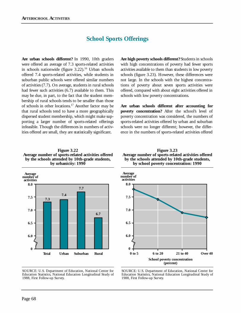
Page 68
AFTERSCHOOL ACTIVITIES
Are urban schools different? In 1990, 10th graderswere offered an average of 7.3 sports-related activitiesin schools nationwide (figure 3.22).16 Urban schoolsoffered 7.4 sports-related activities, while students insuburban public schools were offered similar numbersof activities (7.7). On average, students in rural schoolshad fewer such activities (6.7) available to them. Thismay be due, in part, to the fact that the student mem-bership of rural schools tends to be smaller than thoseof schools in other locations.17 Another factor may bethat rural schools tend to have a more geographicallydispersed student membership, which might make sup-porting a larger number of sports-related offeringsinfeasible. Though the differences in numbers of activ-ities offered are small, they are statistically significant.
Are high poverty schools different? Students in schoolswith high concentrations of poverty had fewer sportsactivities available to them than students in low povertyschools (figure 3.23). However, these differences werenot large. In the schools with the highest concentra-tions of poverty about seven sports activities wereoffered, compared with about eight activities offered inschools with low poverty concentrations.
Are urban schools different after accounting forpoverty concentration? After the school’s level ofpoverty concentration was considered, the numbers ofsports-related activities offered by urban and suburbanschools were no longer different; however, the differ-ence in the numbers of sports-related activities offered
School Sports Offerings
Averagenumber ofactivities
Total Urban Suburban Rural
7.7
6.7
7.37.4
0
6.0
6.5
7.0
7.5
8.0
School poverty concentration(percent)
0 to 5 6 to 20 21 to 40 Over 400
6.0
6.5
7.0
7.5
8.0
Averagenumber ofactivities
Figure 3.22Average number of sports-related activities offeredby the schools attended by 10th-grade students,
by urbanicity: 1990
Figure 3.23Average number of sports-related activities offeredby the schools attended by 10th-grade students,
by school poverty concentration: 1990
SOURCE: U.S. Department of Education, National Center forEducation Statistics, National Education Longitudinal Study of1988, First Follow-up Survey.
SOURCE: U.S. Department of Education, National Center forEducation Statistics, National Education Longitudinal Study of1988, First Follow-up Survey.

AFTERSCHOOL ACTIVITIES
Page 69
by urban and rural schools remained. Fewer activitieswere offered to 10th-grade students in rural schoolsthan in urban schools at every level of poverty concen-tration except the lowest (figure 3.24).
Is the number of sports-related activities lower thanpredicted in urban schools with high concentrationsof poverty? Students in urban high poverty schools hadaccess to a similar number of activities as those in sub-urban high poverty schools (about seven), and slightlymore than rural high poverty schools (about six). The
number of activities in urban high poverty schoolscould be predicted given the patterns for urban schoolsand high poverty schools considered separately. That is,being in a poor urban school did not present any dis-advantage in the number of sports-related activitiesoffered beyond that observed for high poverty schoolsin general.
16Sports-related activities included baseball/softball, basketball,football, soccer, swim team, other team sports, other individualsports, cheerleading, and drill team.
17See chapter 1 above.
Averagenumber ofactivities
0 to 5 6 to 20 21 to 40 Over 40
Suburban
Urban
Rural
0
School poverty concentration(percent)
6.0
6.5
7.0
7.5
8.0
Figure 3.24Average number of sports-related activities offered by the schools attended by 10th-grade students,
by urbanicity and school poverty concentration: 1990
SOURCE: U.S. Department of Education, National Center for Education Statistics, National Education Longitudinal Study of 1988,First Follow-up Survey.

Page 70
AFTERSCHOOL ACTIVITIES
Are urban schools different? In 1990, a little morethan half of all 10th-grade students participated tosome extent in sports-related school activities (figure3.25).18 However, urban students were less likely thaneither suburban or rural students to have participat-ed—45 percent compared with 54 percent and 53percent, respectively.
Are high poverty schools different? Students in highpoverty schools were less likely to participate in schoolsports-related activities than other students (figure3.26). Approximately 56 percent of students in schoolswith low poverty concentrations were involved in
sports-related activities, compared with 44 percent ofstudents in high poverty schools.
Are urban schools different after accounting forpoverty concentration? When the school’s level ofpoverty concentration was taken into account, urbanstudents’ participation rates in sports-related activitiesgenerally remained lower than those of other students(figure 3.27). Among students enrolled in schools withlower poverty concentrations (20 percent or less),urban students tended to be less likely to participate insports-related activities than students in similar subur-ban and rural schools.
Sports Participation
Percent
Total Urban Suburban Rural0
40
45
50
55
60
54.4
52.751.6
45.0
Percent
0
40
45
50
55
60
School poverty concentration(percent)
0 to 5 6 to 20 21 to 40 Over 40
Figure 3.25Percentage of 10th-grade students who participated in sports-related activities,
by urbanicity: 1990
Figure 3.26Percentage of 10th-grade students who participated in sports-related activities,by school poverty concentration: 1990
SOURCE: U.S. Department of Education, National Center forEducation Statistics, National Education Longitudinal Study of1988, First Follow-up Survey.
SOURCE: U.S. Department of Education, National Center forEducation Statistics, National Education Longitudinal Study of1988, First Follow-up Survey.

AFTERSCHOOL ACTIVITIES
Page 71
Is the percentage of students participating in sports-related activities lower than predicted in urban schoolswith high concentrations of poverty? At the highestlevel of poverty concentration, the participation rates ofurban, suburban, and rural students did not differ sig-nificantly. The combination of being in an urban schoolwith a high poverty concentration was not related toany additional disadvantage for these students. That is,
students in these schools participated in sports-relatedactivities at rates that would be predicted for students inschools that were both urban and high poverty.
18Participation was defined as being involved in one or more intra-mural sports, junior varsity, freshman or varsity team sports, orcheerleading or drill teams for such sports.
Figure 3.27Percentage of 10th-grade students who participated in sports-related activities,
by urbanicity and school poverty concentration: 1990
Percent
0 to 5 6 to 20 21 to 40 Over 40
Suburban
Urban
Rural
0
40
45
50
55
60
School poverty concentration(percent)
SOURCE: U.S. Department of Education, National Center for Education Statistics, National Education Longitudinal Study of 1988,First Follow-up Survey.

Page 72
AFTERSCHOOL ACTIVITIES
Employment while attending high school appears tohave both short-term effects upon students’ degree ofengagement in school and long-term effects upon stu-dents’ future labor market activities. While previouslymany researchers had argued that overall students ben-efited from their early labor market experiences(Mangum 1988; Lewin-Epstein 1981), the picture isnot nearly so clear based on recent research(Greenberger and Steinberg 1986).
Many researchers now argue that part-time employ-ment has a deleterious effect on educational outcomesand on future labor market experience. Students whowork during the school year have less time for home-work and may be too tired to accomplish their school
work successfully. In addition, as students becomemore involved in the labor force, they may become lessinterested in school. In terms of future labor marketexperiences, the downside to part-time employmentwas unforeseen during the 1970s. The reality is thatmost part-time jobs currently available to students arehigh stress, dead-end jobs (store clerk, food serviceworker), which actually promote delinquent behaviorsand encourage students to develop negative attitudestoward work itself (Greenberger and Steinberg 1986).
Some research (Newmann 1992) has found that stu-dents who work 20 or more hours per week are morelikely to experience negative effects from working. Inthis section, the measure examined is whether or not
Employment of 10th-Grade Students
Percent
Total Urban Suburban Rural0
5
10
15
20
25
19.9
16.818.4 18.3
Percent
0
5
10
15
20
25
School poverty concentration(percent)
0 to 5 6 to 20 21 to 40 Over 40
Figure 3.28Percentage of 10th-grade students who worked
11 or more hours per week, by urbanicity: 1990
Figure 3.29Percentage of 10th-grade students who worked
11 or more hours per week, by school poverty concentration: 1990
SOURCE: U.S. Department of Education, National Center forEducation Statistics, National Education Longitudinal Study of1988, First Follow-up Survey.
SOURCE: U.S. Department of Education, National Center forEducation Statistics, National Education Longitudinal Study of1988, First Follow-up Survey.

AFTERSCHOOL ACTIVITIES
10th-grade students work 11 or more hours per weekduring the school year, because few students in the10th grade work 20 hours or more per week.
Are urban schools different? In 1990, about 18 percentof 10th graders were employed 11 or more hours perweek (figure 3.28). However, urban 10th graders werejust as likely as other students to be working this manyhours. While it appears that rural students were lesslikely than urban students to work 11 or more hours,this difference is not statistically significant.
Are high poverty schools different? While the propor-tions of urban, suburban, and rural students whoworked 11 or more hours varied little, the proportions
of such students did vary according to the level ofpoverty concentration in the school (figure 3.29). Alower proportion of students in schools with the high-est concentration of poverty worked 11 or more hoursthan students in schools with lower poverty concentra-tions (20 percent or less). For example, about 14percent of students in schools with the highest povertyconcentration worked 11 or more hours, comparedwith about 20 percent of 10th graders attendingschools with less than 20 percent poverty concentra-tion. For students in schools with the highest and nextto highest poverty concentrations, however, there wasno statistically significant difference in their likelihoodof working.
Page 73
Figure 3.30Percentage of 10th-grade students who worked 11 or more hours per week,
by urbanicity and school poverty concentration: 1990
Percent
0 to 5 6 to 20 21 to 40 Over 40
Suburban
Urban Rural
0
5
10
15
20
25
School poverty concentration(percent)
SOURCE: U.S. Department of Education, National Center for Education Statistics, National Education Longitudinal Study of 1988,First Follow-up Survey.

Are urban schools different after accounting forpoverty concentration? There were no significant dif-ferences by urbanicity after taking into account povertyconcentration.
Is the percentage of students who work part timehigher than predicted in urban schools with high
concentrations of poverty? Students in urban highpoverty schools were as likely to be employed as thosein other high poverty schools, and their employmentlevels could be predicted from the combination oflocation and level of poverty concentration (figure3.30).
Page 74
AFTERSCHOOL ACTIVITIES

The national interest in developing programs toimprove the schooling and educational outcomes ofchildren attending urban public schools and particular-ly high poverty urban schools has never been greater.Many authors have debated how resources contribute todifferences in the quality of the educational experiencesfound in urban schools generally and, particularly, inthose that serve poor students.19 This chapter con-tributes to that debate by presenting empirical evidencefrom nationally representative surveys to show whetherand how the school experiences of these children differfrom those of other students.
This chapter addresses three key areas that affect achild’s public school experience: school resources andstaff, school programs and coursetaking, and studentbehavior. Meaningful differences in these areas betweenschools in different locations lend support to the con-tention that some groups of students have less desirableeducational experiences and more limited opportuni-ties than other groups. These differences may berelated, in turn, to the poorer outcomes for somegroups of students observed in chapter 2. Further, theycan help focus the national policy and research agendaon those areas that need to be improved for studentsattending high poverty public schools in urban locations.
The same analysis model that was used in previouschapters is used in this chapter to distinguish differ-ences by school urbanicity and poverty concentration,separately and in combination with one another.Schools and students were grouped according to theurbanicity and level of poverty concentration in theschool. Specifically, the analysis determines:
1) whether students’ school experiences differ bylocation;
2) whether their school experiences differ by schoolpoverty concentration;
3) whether differences by school location remainafter accounting for the variation in schoolpoverty concentration; and
4) whether the school experiences of students inurban high poverty schools differs from that ofstudents in high poverty schools in other loca-tions, and whether urban high poverty schoolsare different than predicted on the measuresexamined.
The phrase greater than predicted means that the differ-ences between urban high poverty and other schoolswere larger than would be predicted from the additiveeffects of an urban and high poverty setting, indicatingan interaction, or compounding effect, of the two. Thischapter presents data separately for elementary and sec-ondary schools when there are meaningful differencesby level.
Current measures of school quality that are available innational surveys reflect neither the depth nor breadthof a student’s school experiences (Bobbitt et al. 1992).Thus, the indicators presented in this chapter are lim-ited by the available data and do not provide athorough review of student experiences. Rather, theyare a selective set of indicators for public schools andstudents. These indicators were chosen through aprocess that included a review of available data andresearch to identify important aspects of the schoolenvironment and an analysis that revealed those indica-tors that varied meaningfully by location and level ofpoverty in the school (see appendix C for a list of datareviewed).
Chart 4.1 displays the indicators for the three sectionsin this chapter—school resources and staff, school pro-grams and coursetaking, and student behavior—as well
Page 75
Chapter 4
School Experiences
19For example, Hedges, Laine, and Greenwald April 1994;Hanushek 1994; Hedges, Laine, and Greenwald May 1994.

as the results of the analyses (discussed in the next sec-tion). First, the school resources and staff sectionaddresses the issue of the distribution of financialresources through teachers’ rating of the adequacy ofschool resources and teacher salaries. The experienceand availability of teachers are measured by years ofteaching experience and the difficulties that adminis-trators encounter in hiring teachers. Next, thedemographics of the teaching force are characterized bythe percentage of teachers who are minority and male.Finally, this section presents data on teachers’ influenceover the curricula they teach and teacher absenteeism asindicators of the control that teachers have over theirwork and teacher morale.
The second section presents indicators of student par-ticipation in public school programs and studentcoursetaking in four areas: preschool attendance, avail-ability of gifted and talented programs, participation invocational education, and mathematics coursetaking(geometry).
Finally, the third section presents indicators of studentbehaviors, both in and out of school, that affect theiracademic performance. Behaviors of individual stu-dents can affect their own as well as other students’academic performance. The first group presented arethose that affect one’s own performance: the amount oftime spent doing homework, the amount of televisionwatched on weekdays, and absenteeism from school.The second group reflect the influence of the classroomand school environment: the amount of time teachersspend maintaining discipline in the classroom, and stu-dents’ perception of their own safety and the threat ofweapons in their schools. Finally, this section presentstwo additional risk-taking behaviors outside of schoolthat affect academic performance and completion: stu-dents’ use of alcohol, and pregnancy.
Chart 4.1 reports the answers to the questions thatwere asked of the data for each indicator of schoolexperience. Although the table presents the results ofthe complete analysis, this discussion will focus onthe questions in the third and fourth columns: Are
urban public schools different after accounting forthe higher poverty concentration in urban schools?Are urban high poverty schools different from subur-ban and rural high poverty schools? Are the schoolexperiences of students in urban high poverty schoolsdifferent than predicted?
Summary of This Chapter’s Findings
• Students in urban public schools overall had lessdesirable experiences than those in other loca-tions on 8 of the 20 measures analyzed, evenafter accounting for the higher poverty concen-tration in urban schools.
• Students in public schools with high povertyconcentrations had less desirable school experi-ences than those in low poverty schools on everymeasure except the availability of minority staffand student use of alcohol.
• Students in high poverty urban public schoolshad less desirable school experiences than thosein high poverty rural schools on nearly half of themeasures, and had less desirable experiences thanthose in high poverty suburban schools on twoof the indicators.
• Students in high poverty urban schools hadunusually high rates of television watching com-pared with other groups of students, exceedingthe rates that would be predicted from the dif-ferences by location and poverty concentrationcombined.
• Among the school resources and staff indicators,fewer necessary resources for teachers, hiring dif-ficulties, lack of teacher influence overcurriculum, and higher teacher absenteeism wereproblems affecting urban schools more than sub-urban and rural schools, and urban high povertyschools more than rural high poverty schools.However, urban high poverty schools had a morediverse staff than other schools, and more minor-
Page 76

ity teachers than would be predicted from thecombination of their location and poverty con-centration compared with rural schools.
• School program and coursetaking indicators sug-gest that students in urban schools, overall, wereat a disadvantage compared with those in subur-ban schools in their access to gifted and talentedprograms, but this disadvantage did not hold forurban high poverty schools compared with similarsuburban schools.
• With regard to the other school program andcoursetaking indicators—preschool attendance,participation in vocational education, and mathe-matics coursetaking—students in urban publicschools, after accounting for poverty, and in urbanhigh poverty schools were no different than others.
Moreover, both students in urban and urban highpoverty schools had higher preschool attendancerates than their rural counterparts.
• In the area of student behavior, absenteeism, classdiscipline, feeling safe at school, weapons posses-sion, and pregnancy were more likely to beproblems among urban students overall thanamong other students.
• In general, students in urban high poverty schoolshad more disciplinary problems and were muchmore likely to watch a lot of television. Otherwise,they behaved similarly to their suburban and ruralcounterparts with two exceptions: they were morelikely to be absent than rural students, andweapons possession was more likely to be a prob-lem in their schools than in rural schools.
Page 77
Are Urban Are High Are Urban Are Urban HighSchools Poverty Schools Schools Poverty SchoolsDifferent? Different? Different after Different from
Accounting for Other HighPoverty Poverty Schools?Concentration?
Are Urban HighPoverty SchoolsDifferent than
INDICATOR Predicted?
I. SCHOOL RESOURCES AND STAFF
Necessary Yes, Yes, Yes, Yes, Resources urban lower than high poverty lower urban lower than lower than ruralAvailable suburban and rural than all others others high poverty, same
as suburban highpoverty
No differentthan predicted
Teacher Yes, Yes, Yes, Yes,Salary urban higher than high poverty lower urban higher than higher than rural
rural, lower than than most others rural, same as high poverty, samesuburban suburban as suburban high
poverty
No differentthan predicted
CHART 4.1—SUMMARY OF RESULTS: SCHOOL EXPERIENCES
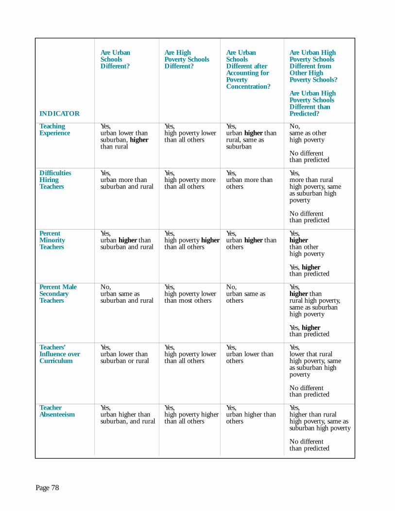
Page 78
Are Urban Are High Are Urban Are Urban HighSchools Poverty Schools Schools Poverty SchoolsDifferent? Different? Different after Different from
Accounting for Other HighPoverty Poverty Schools?Concentration?
Are Urban HighPoverty SchoolsDifferent than
INDICATOR Predicted?
Teaching Yes, Yes, Yes, No,Experience urban lower than high poverty lower urban higher than same as other
suburban, higher than all others rural, same as high povertythan rural suburban
No differentthan predicted
Difficulties Yes, Yes, Yes, Yes,Hiring urban more than high poverty more urban more than more than ruralTeachers suburban and rural than all others others high poverty, same
as suburban highpoverty
No differentthan predicted
Percent Yes, Yes, Yes, Yes,Minority urban higher than high poverty higher urban higher than higherTeachers suburban and rural than all others others than other
high poverty
Yes, higherthan predicted
Percent Male No, Yes, No, Yes, Secondary urban same as high poverty lower urban same as higher thanTeachers suburban and rural than most others others rural high poverty,
same as suburbanhigh poverty
Yes, higherthan predicted
Teachers’ Yes, Yes, Yes, Yes, Influence over urban lower than high poverty lower urban lower than lower that ruralCurriculum suburban or rural than all others others high poverty, same
as suburban highpoverty
No differentthan predicted
Teacher Yes, Yes, Yes, Yes,Absenteeism urban higher than high poverty higher urban higher than higher than rural
suburban, and rural than all others others high poverty, same assuburban high poverty
No differentthan predicted

Page 79
Are Urban Are High Are Urban Are Urban HighSchools Poverty Schools Schools Poverty SchoolsDifferent? Different? Different after Different from
Accounting for Other HighPoverty Poverty Schools?Concentration?
Are Urban HighPoverty SchoolsDifferent than
INDICATOR Predicted?
II. SCHOOL PROGRAMS AND COURSETAKING
Preschool Yes, Yes, Yes, Yes,Attendance urban lower than high poverty lower urban higher than higher than ruralRates suburban, higher than all others rural, same as high poverty, same
than rural suburban suburban high poverty
No differentthan predicted
Gifted and Yes, Yes, Yes, Yes,Talented urban lower than high poverty lower urban lower than lower that ruralPrograms suburban, same as than all others suburban, same as high poverty, same
rural rural as suburban highpoverty
Yes, lowerthan predicted
Vocational No, Yes, No, *Education urban same as higher as poverty urban same as No differentCredits suburban and rural increases* others than predicted
Percentage of Yes, Yes, No, *Seniors Who urban lower than lower as poverty urban same as No differentTook Geometry suburban, same as increases* others than predicted
rural
III. STUDENT BEHAVIOR
Television Yes, Yes, No, Yes, Watching on urban higher than high poverty higher urban same as higher than otherWeekdays suburban, same as than all others others high poverty
ruralYes, higherthan predicted
Hours of No, Yes, No, No,Homework urban same as high poverty lower urban same as same as other highCompleted suburban and rural than all others others poverty
No differentthan predicted
*This indicator was tested using poverty concentration as a continuous rather than categorical variable. Since the sample sizes for schools byurbanicity and poverty concentration combined were too small to produce reliable estimates, no comparisons were made between urban highpoverty and other high poverty schools.

Page 80
Are Urban Are High Are Urban Are Urban HighSchools Poverty Schools Schools Poverty SchoolsDifferent? Different? Different after Different from
Accounting for Other HighPoverty Poverty Schools?Concentration?
Are Urban HighPoverty SchoolsDifferent than
INDICATOR Predicted?
Student Yes, Yes, Yes, Yes,Absenteeism higher than high poverty higher urban higher than higher than rural high
suburban than all others others poverty, same assuburban high poverty
No differentthan predicted
Time Yes, Yes, Yes, Yes,Maintaining urban higher than high poverty higher urban higher than higher thanDiscipline suburban and rural than most others others other high poverty
No differentthan predicted
Feeling Yes, Yes, Yes, No,Unsafe in urban higher than high poverty higher urban higher same as otherSchool suburban and rural than most others than rural, same as high poverty
suburbanNo differentthan predicted
Student Yes, Yes, Yes, Yes,Weapons urban higher than high poverty higher urban higher than higher than ruralPossession suburban and rural than all others others high poverty, same
as suburban highpoverty
No differentthan predicted
Student Yes, Yes, Yes, No,Use of urban lower than high poverty lower urban lower than same as otherAlcohol suburban and rural than all others rural, same as high poverty
suburbanNo differentthan predicted
Student Yes, Yes, Yes, No,Pregnancy urban higher than high poverty higher urban higher than same as other
suburban, and rural than all others others high poverty
No differentthan predicted

Adequate resources and a committed, well-qualified,and professional staff of teachers are key elements of avital learning environment which leads to high acade-mic achievement (Special Study Panel on EducationIndicators 1991). Yet urban high poverty publicschools are often assumed to have fewer well-qualifiedteachers and fewer resources—issues that strike at theheart of what it means to provide high-quality educa-tion for all youngsters.
This section examines three aspects of school resourcesand staffing: availability of resources and teachersalaries, teacher experience and supply, and teachercharacteristics and behavior. Each indicator has beenselected for its relevance to policy debates about thequality of the school environment, but the indicatorspresented are by no means exhaustive.20
Findings
• Public urban schools did less well in providingnecessary resources to teachers, and urban highpoverty public schools did less well in this areathan rural high poverty schools. However, urbanteacher salaries were, in fact, higher than thosefor rural teachers. Teachers in high poverty urbanschools also had higher salaries than their ruralcounterparts, and had about the same salaries asthose in suburban high poverty schools.
• Teachers in urban public schools, after account-ing for poverty, and urban high poverty schoolswere just as experienced as their suburban andrural counterparts. In fact, urban teachers, over-
all, were more experienced than rural teachers.However, administrators of urban schools, ingeneral, and urban high poverty schools in par-ticular, were more apt to complain aboutdifficulties in hiring qualified teachers than mostother administrators.
• Teachers in urban and urban high poverty pub-lic schools were more likely to be minorities, butjust as likely to be male as those in comparableschools in other locations. In fact, teachers inurban high poverty schools were more likely tobe male than those in rural high poverty schools.
• Urban teachers and those in urban high povertyschools reported less influence over their curricu-lum than most teachers in other locations.Teachers’ perceptions of the level of teacherabsenteeism were higher among urban teachersthan among teachers in other locations, evenafter taking poverty into account; however,teachers in urban high poverty schools did notconsider teacher absenteeism more serious thanthose in suburban high poverty schools.
• Higher concentrations of poverty in schools hada consistent and pervasive relationship to poorerquality resources and staff. Only one resourceand staffing indicator was favorable in highpoverty schools: there were higher percentages ofminority staff.
Page 81
School Resources and Staff
20See appendix C for a discussion of the criteria used in selectingindicators.

The issue of how school financial resources are distrib-uted is controversial, with some arguing that theamount of expenditures has little effect on student out-comes (Hanushek 1989). Others have reported thatschool finances do make a difference (Rotberg 1993;Berliner 1993). According to a recent report from theCouncil of the Great City Schools, the average perpupil expenditure for large city public school studentswas less than the national average and was also less thanthe expenditure in suburban and rural public schooldistricts (Council of the Great City Schools 1992).
National data on school finance were not available bythe classifications of school location and poverty con-centration required for this analysis. In addition,public school finances are determined primarily atthe district level and are reported by district innational surveys.21 Both the urbanicity and poverty
concentration of schools can vary within a school dis-trict, as do expenditures and resource availability.
The school-level indicator presented in this section isderived from teacher opinion data on the availability ofnecessary materials (e.g., textbooks, supplies, copymachines) for the staff. Teacher responses can providean indication of resource availability at the school levelsince teachers may be in the best position to judgewhether the resources available in the school are ade-quate to meet the demands of instruction.
Are urban schools different? Seventy-six percent ofpublic school teachers nationwide agreed that necessarymaterials were available in their schools in 1987–88.However, urban teachers were less likely to report thatneeded materials were available than teachers in eithersuburban or rural schools (figure 4.1). Seventy percent
Page 82
SCHOOL RESOURCES AND STAFF
Availability of Resources
Percent
Total Urban Suburban Rural0
50
60
70
80
90
79.3 78.076.3
70.1
Percent
0
50
60
70
80
90
School poverty concentration(percent)
0 to 5 6 to 20 21 to 40 Over 40
Figure 4.1Percentage of teachers who agreed that necessary
materials are available in their schools,by urbanicity: 1987–88
Figure 4.2Percentage of teachers who agreed that necessary
materials are available in their schools,by school poverty concentration: 1987–88
SOURCE: U.S. Department of Education, National Center forEducation Statistics, Schools and Staffing Survey, 1987–88,Teacher File.
SOURCE: U.S. Department of Education, National Center forEducation Statistics, Schools and Staffing Survey, 1987–88,Teacher File.

of urban teachers reported that materials were adequatecompared with 79 percent of suburban and 78 percentof rural teachers.
Are schools with high poverty concentrations different?There were also differences by concentration of pover-ty in the schools. Teachers in schools with the highestconcentration of poverty reported less frequently thanteachers in any other school type that the resourcesavailable to the staff were adequate (72 percent com-pared with 80 percent of teachers in the low povertyschools) (figure 4.2).
Are urban schools different after accounting for thepoverty concentration of the school? After accountingfor differences in poverty concentration across schoollocales, teachers in urban schools were still less likely toreport that necessary materials were available (figure4.3). That is, the fact that urban schools are more like-
ly to have high concentrations of poverty is not theonly explanation for why urban teachers were less like-ly to feel that resources were adequate.
Were teachers from urban high poverty schools lesslikely to have necessary materials than predicted?Teachers in urban high poverty schools were less likelyto feel they had necessary materials than teachers inevery other school type with the exception of teachersin suburban high poverty schools. Sixty-seven percentof teachers in urban high poverty schools felt thatresources were adequate. However, an urban locationand a high poverty concentration do not combine tocreate any additional disadvantage above and beyondthat observed separately for urban teachers and teach-ers in high poverty schools.
Page 83
SCHOOL RESOURCES AND STAFF
21An interesting discussion on the differences in spendingbetween districts can be found in William T. Hartman (Spring1988, 436–459).
Figure 4.3Percentage of teachers who agreed that necessary materials are available in their schools,
by urbanicity and school poverty concentration: 1987–88
Percent
Suburban
Urban
Rural
0
50
60
70
80
90
School poverty concentration(percent)
0 to 5 6 to 20 21 to 40 Over 40
SOURCE: U.S. Department of Education, National Center for Education Statistics, Schools and Staffing Survey, 1987–88, Teacher File.
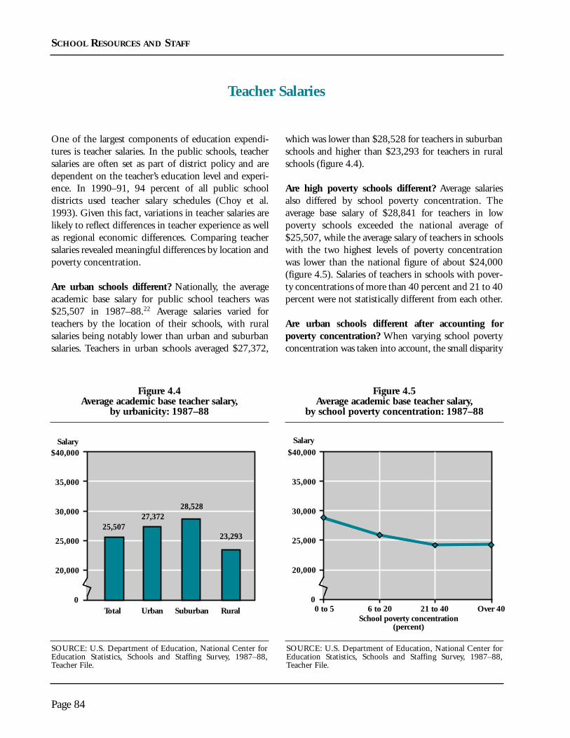
One of the largest components of education expendi-tures is teacher salaries. In the public schools, teachersalaries are often set as part of district policy and aredependent on the teacher’s education level and experi-ence. In 1990–91, 94 percent of all public schooldistricts used teacher salary schedules (Choy et al.1993). Given this fact, variations in teacher salaries arelikely to reflect differences in teacher experience as wellas regional economic differences. Comparing teachersalaries revealed meaningful differences by location andpoverty concentration.
Are urban schools different? Nationally, the averageacademic base salary for public school teachers was$25,507 in 1987–88.22 Average salaries varied forteachers by the location of their schools, with ruralsalaries being notably lower than urban and suburbansalaries. Teachers in urban schools averaged $27,372,
which was lower than $28,528 for teachers in suburbanschools and higher than $23,293 for teachers in ruralschools (figure 4.4).
Are high poverty schools different? Average salariesalso differed by school poverty concentration. Theaverage base salary of $28,841 for teachers in lowpoverty schools exceeded the national average of$25,507, while the average salary of teachers in schoolswith the two highest levels of poverty concentrationwas lower than the national figure of about $24,000(figure 4.5). Salaries of teachers in schools with pover-ty concentrations of more than 40 percent and 21 to 40percent were not statistically different from each other.
Are urban schools different after accounting forpoverty concentration? When varying school povertyconcentration was taken into account, the small disparity
Page 84
SCHOOL RESOURCES AND STAFF
Teacher Salaries
Salary
Total Urban Suburban Rural0
20,000
25,000
30,000
35,000
$40,000
25,50727,372
23,293
28,528
Salary
0
20,000
25,000
30,000
35,000
$40,000
School poverty concentration(percent)
0 to 5 6 to 20 21 to 40 Over 40
Figure 4.4Average academic base teacher salary,
by urbanicity: 1987–88
Figure 4.5Average academic base teacher salary,
by school poverty concentration: 1987–88
SOURCE: U.S. Department of Education, National Center forEducation Statistics, Schools and Staffing Survey, 1987–88,Teacher File.
SOURCE: U.S. Department of Education, National Center forEducation Statistics, Schools and Staffing Survey, 1987–88,Teacher File.
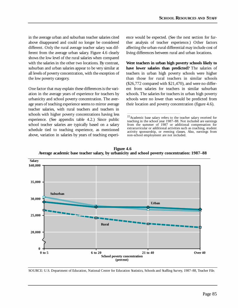
in the average urban and suburban teacher salaries citedabove disappeared and could no longer be considereddifferent. Only the rural average teacher salary was dif-ferent from the average urban salary. Figure 4.6 clearlyshows the low level of the rural salaries when comparedwith the salaries in the other two locations. By contrast,suburban and urban salaries appear to be very similar atall levels of poverty concentration, with the exception ofthe low poverty category.
One factor that may explain these differences is the vari-ation in the average years of experience for teachers byurbanicity and school poverty concentration. The aver-age years of teaching experience seems to mirror averageteacher salaries, with rural teachers and teachers inschools with higher poverty concentrations having lessexperience. (See appendix table 4.2.) Since publicschool teacher salaries are typically based on a salaryschedule tied to teaching experience, as mentionedabove, variation in salaries by years of teaching experi-
ence would be expected. (See the next section for fur-ther analysis of teacher experience.) Other factorsaffecting the urban-rural differential may include cost ofliving differences between rural and urban locations.
Were teachers in urban high poverty schools likely tohave lower salaries than predicted? The salaries ofteachers in urban high poverty schools were higherthan those for rural teachers in similar schools($26,772 compared with $21,470), and were no differ-ent from salaries for teachers in similar suburbanschools. The salaries for teachers in urban high povertyschools were no lower than would be predicted fromtheir location and poverty concentration (figure 4.6).
Page 85
SCHOOL RESOURCES AND STAFF
22Academic base salary refers to the teacher salary received forteaching in the school year 1987–88. Not included are earningsfrom the summer of 1987 or additional compensation forextracurricular or additional activities such as coaching, studentactivity sponsorship, or evening classes. Also, earnings fromnon-school employment are not included.
Figure 4.6Average academic base teacher salary, by urbanicity and school poverty concentration: 1987–88
0 to 5 6 to 20 21 to 40 Over 40
Suburban
Urban
Rural
0
School poverty concentration(percent)
Salary
20,000
25,000
30,000
35,000
$40,000
SOURCE: U.S. Department of Education, National Center for Education Statistics, Schools and Staffing Survey, 1987–88, Teacher File.
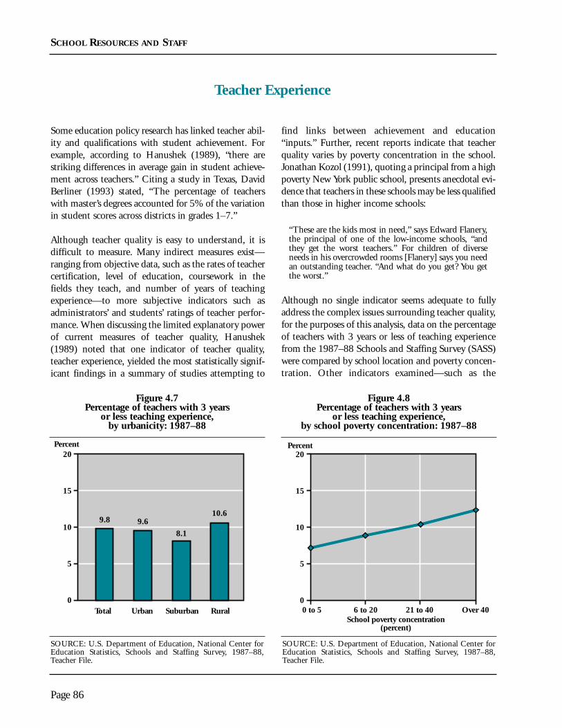
Some education policy research has linked teacher abil-ity and qualifications with student achievement. Forexample, according to Hanushek (1989), “there arestriking differences in average gain in student achieve-ment across teachers.” Citing a study in Texas, DavidBerliner (1993) stated, “The percentage of teacherswith master’s degrees accounted for 5% of the variationin student scores across districts in grades 1–7.”
Although teacher quality is easy to understand, it isdifficult to measure. Many indirect measures exist—ranging from objective data, such as the rates of teachercertification, level of education, coursework in thefields they teach, and number of years of teachingexperience—to more subjective indicators such asadministrators’ and students’ ratings of teacher perfor-mance. When discussing the limited explanatory powerof current measures of teacher quality, Hanushek(1989) noted that one indicator of teacher quality,teacher experience, yielded the most statistically signif-icant findings in a summary of studies attempting to
find links between achievement and education“inputs.” Further, recent reports indicate that teacherquality varies by poverty concentration in the school.Jonathan Kozol (1991), quoting a principal from a highpoverty New York public school, presents anecdotal evi-dence that teachers in these schools may be less qualifiedthan those in higher income schools:
“These are the kids most in need,” says Edward Flanery,the principal of one of the low-income schools, “andthey get the worst teachers.” For children of diverseneeds in his overcrowded rooms [Flanery] says you needan outstanding teacher. “And what do you get? You getthe worst.”
Although no single indicator seems adequate to fullyaddress the complex issues surrounding teacher quality,for the purposes of this analysis, data on the percentageof teachers with 3 years or less of teaching experiencefrom the 1987–88 Schools and Staffing Survey (SASS)were compared by school location and poverty concen-tration. Other indicators examined—such as the
Page 86
SCHOOL RESOURCES AND STAFF
Teacher Experience
Percent
Total Urban Suburban Rural0
5
10
15
20
8.1
10.69.8 9.6
Percent
School poverty concentration(percent)
0 to 5 6 to 20 21 to 40 Over 400
5
10
15
20
Figure 4.7Percentage of teachers with 3 years
or less teaching experience,by urbanicity: 1987–88
Figure 4.8Percentage of teachers with 3 years
or less teaching experience,by school poverty concentration: 1987–88
SOURCE: U.S. Department of Education, National Center forEducation Statistics, Schools and Staffing Survey, 1987–88,Teacher File.
SOURCE: U.S. Department of Education, National Center forEducation Statistics, Schools and Staffing Survey, 1987–88,Teacher File.

percentage of teachers who were certified, the numberof courses they took in their main assignment field, andteacher degree attainment—did not reveal much varia-tion by urbanicity or school poverty concentration.(See appendix C.)
Are urban schools different? On average, 10 percent ofpublic school teachers nationwide had 3 years or lessteaching experience in the 1987–88 school year. Tenpercent of urban teachers had 3 years or less experience,which was greater than the 8 percent for suburbanteachers but less than the 11 percent for rural teachers(figure 4.7).
Are high poverty schools different? The number ofyears of teaching experience varied by school povertyconcentration (figure 4.8). High poverty schools hadthe highest percentage of teachers with 3 years or lessteaching experience (12 percent), which was 70 percenthigher than that of low poverty schools (7 percent).
Are urban schools different after accounting for povertyconcentration? Once the association between the schools’poverty concentration and teacher experience was takeninto account, there was no difference between urban andsuburban schools in teacher experience. The rural-urbandifference, remained, however. As shown in figure 4.9,the urban and suburban percentages are very close at alllevels of school poverty, while rural schools have a greaterproportion of less experienced teachers in general.
Were teachers in urban high poverty schools more like-ly to have 3 years or less teaching experience than wouldbe predicted? Urban teachers in high poverty schoolswere as likely as predicted to have 3 years or less teachingexperience. In fact, the percentage of these teachers hav-ing less than 4 years of teaching experience (12 percent)was no different than in high poverty schools in otherlocations. The relatively high percentage of less experi-enced teachers in urban high poverty schools reflects thehigh poverty concentration of their schools, not theurban location (figure 4.9).
Page 87
SCHOOL RESOURCES AND STAFF
Figure 4.9Percentage of teachers with 3 years or less teaching experience,
by urbanicity and school poverty concentration: 1987–88
Percent
0 to 5 6 to 20 21 to 40 Over 40
Suburban
Urban
Rural
0
5
10
15
20
School poverty concentration(percent)
SOURCE: U.S. Department of Education, National Center for Education Statistics, Schools and Staffing Survey, 1987–88, Teacher File.

Although predicted teacher shortages did not material-ize in the late 1980s (Bobbitt 1991), reports persist thatshortages of well-qualified teachers exist for schools inthe inner cities serving large numbers of disadvantagedchildren (Oakes 1990). This section looks at evidencethat the supply of teachers may vary by urbanicity andschool type. The indicator below, drawn from the1987–88 SASS, compares administrator reports of havinggeneral difficulties hiring teachers for their schools.23
Are urban schools different? Nationally, 16 percent ofpublic school administrators reported that they expe-rienced general difficulties hiring teachers whensurveyed in 1987–88. For urban schools, this per-centage was much higher (23 percent) than it was forsuburban and rural schools, which were both at 13percent (figure 4.10).
Are high poverty schools different? Administratorsfrom high poverty schools were more likely than theirpeers in other schools to have difficulty hiring teachers.Twenty-four percent of the administrators from thehighest poverty schools reported having difficulties—twice the proportion of the administrators from thelower poverty schools (those with 0–5 percent and6–20 percent poverty concentration) and somewhatless than twice the proportion when compared withadministrators from schools with 21–40 percent pover-ty concentration (figure 4.11).
Are urban schools different after accounting forpoverty concentration? The differences between thehigh poverty schools and all other school types werequite large, and when the poverty concentration ofschools in each location was taken into account, the
Page 88
SCHOOL RESOURCES AND STAFF
Difficulty Hiring Teachers
Percent
Total Urban Suburban Rural0
10
20
40
13.2 13.415.7
23.2
30
Percent
School poverty concentration(percent)
0 to 5 6 to 20 21 to 40 Over 400
10
20
40
30
Figure 4.10Percentage of principals who report
difficulty hiring teachers,by urbanicity: 1987–88
Figure 4.11Percentage of principals who report
difficulty hiring teachers,by school poverty concentration: 1987–88
SOURCE: U.S. Department of Education, National Center forEducation Statistics, Schools and Staffing Survey, 1987–88,Administrator File.
SOURCE: U.S. Department of Education, National Center forEducation Statistics, Schools and Staffing Survey, 1987–88,Administrator File.
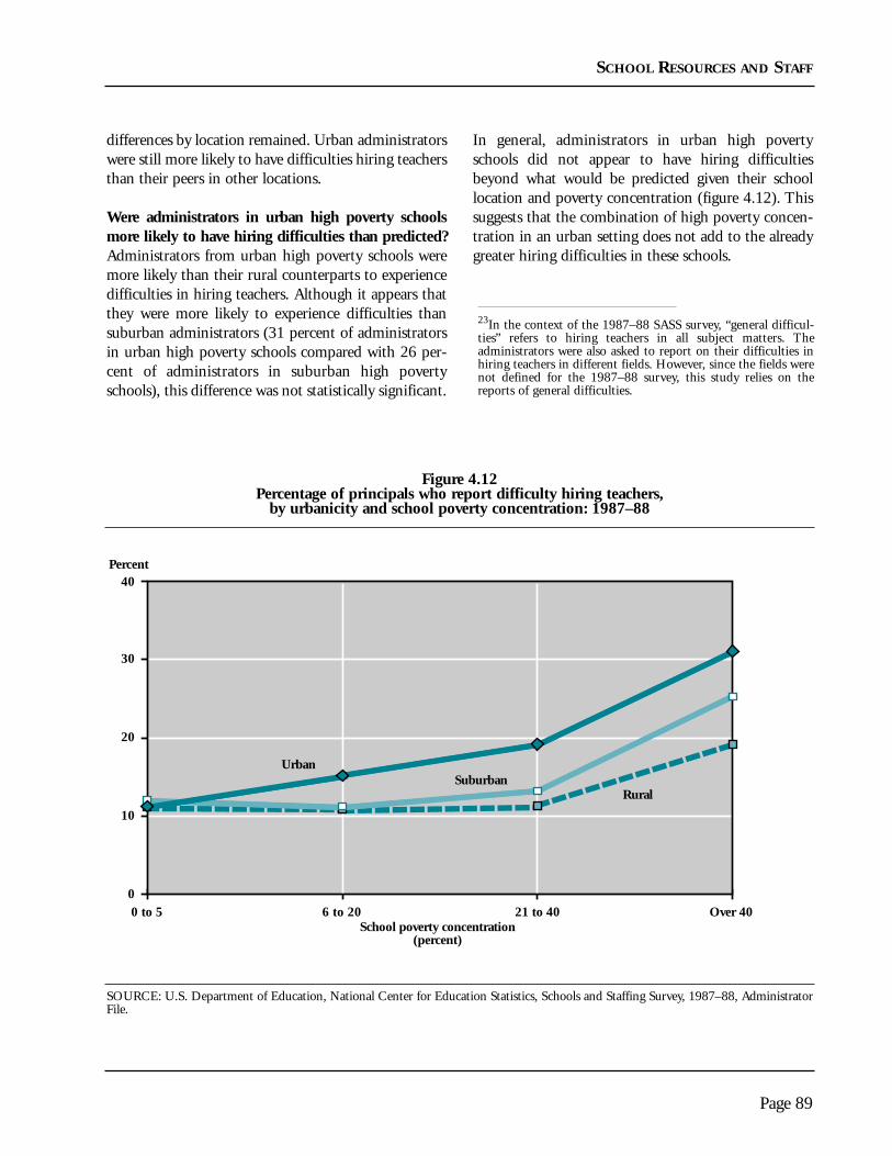
differences by location remained. Urban administratorswere still more likely to have difficulties hiring teachersthan their peers in other locations.
Were administrators in urban high poverty schoolsmore likely to have hiring difficulties than predicted?Administrators from urban high poverty schools weremore likely than their rural counterparts to experiencedifficulties in hiring teachers. Although it appears thatthey were more likely to experience difficulties thansuburban administrators (31 percent of administratorsin urban high poverty schools compared with 26 per-cent of administrators in suburban high povertyschools), this difference was not statistically significant.
In general, administrators in urban high povertyschools did not appear to have hiring difficultiesbeyond what would be predicted given their schoollocation and poverty concentration (figure 4.12). Thissuggests that the combination of high poverty concen-tration in an urban setting does not add to the alreadygreater hiring difficulties in these schools.
Page 89
SCHOOL RESOURCES AND STAFF
23In the context of the 1987–88 SASS survey, “general difficul-ties” refers to hiring teachers in all subject matters. Theadministrators were also asked to report on their difficulties inhiring teachers in different fields. However, since the fields werenot defined for the 1987–88 survey, this study relies on thereports of general difficulties.
Figure 4.12Percentage of principals who report difficulty hiring teachers,
by urbanicity and school poverty concentration: 1987–88
Percent
SuburbanUrban
Rural
0
10
20
40
School poverty concentration(percent)
30
0 to 5 6 to 20 21 to 40 Over 40
SOURCE: U.S. Department of Education, National Center for Education Statistics, Schools and Staffing Survey, 1987–88, AdministratorFile.

In chapter 1, it was shown that minority student enroll-ment is largest in high poverty urban schools. Urbanschools, overall, are also more likely to serve greaterpercentages of minority students than rural and subur-ban schools. Even though researchers have debated thisissue, policymakers are interested in the possible linkbetween having strong minority representation amongteachers and the high achievement and aspirations ofminority students (King 1993). Recent reports suggestthat the number of minority teachers in the publicschools has not risen to meet the level of minority stu-dent enrollment. According to the Vice President of theNational Education Association, teacher recruitmenthas not met the demands of creating a more diversifiedteaching force:
It’s very disheartening to see that we have not madesignificant progress in these areas of teacher recruitment.. . . Students learn lessons about life both through for-mal instruction and what they see around them. Weneed more male elementary school teachers and morepeople of color at all grade levels (Jordan 1992).
A recent report by the Council of the Great CitySchools (1992) also noted,
[T]he demography of urban teachers does not matchthat of urban students . . . viewed from a different angle,these demographic patterns meant that there was oneAfrican-American teacher for every 25.4 African-American students in the Great City Schools, one whiteteacher for every 7.4 white students, one Hispanicteacher for every 62.9 Hispanic students, one Asian-American teacher for every 46.2 Asian-Americanstudents (see also King 1993).
Given student demographics, are schools in urban loca-tions and those with high poverty concentrations morelikely to employ greater numbers of teachers fromminority backgrounds? The 1987–88 SASS askedschools to list the racial-ethnic backgrounds of allteachers using the categories of black non-Hispanic,white non-Hispanic, Native American, Asian or PacificIslander, and Hispanic origin regardless of race. Anindicator of the percentage of teachers who were mem-bers of a racial-ethnic minority was created by
Page 90
SCHOOL RESOURCES AND STAFF
Percent Minority Teachers
Percent
Total Urban Suburban Rural0
10
20
30
40
10.18.1
13.3
28.5
Percent
School poverty concentration(percent)
0 to 5 6 to 20 21 to 40 Over 400
10
20
30
40
Figure 4.13Percentage of teachers who are minority,
by urbanicity: 1987–88
Figure 4.14Percentage of teachers who are minority,
by school poverty concentration: 1987–88
SOURCE: U.S. Department of Education, National Center forEducation Statistics, Schools and Staffing Survey, 1987–88,Teacher File.
SOURCE: U.S. Department of Education, National Center forEducation Statistics, Schools and Staffing Survey, 1987–88,Teacher File.

combining all of the categories with the exception ofwhite, non-Hispanic.
Are urban schools different? Nationally, 13 percent ofthe total public school teaching force in 1987–88 identi-fied with a race-ethnicity other than white. Thepercentage of minority teachers in urban schools wasalmost three times higher (29 percent) than that of sub-urban schools (10 percent), and more than three timeshigher than that of rural schools (8 percent) (figure 4.13).In comparison, the percentage of minority studentsenrolled in urban schools was almost twice as high as thepercentage of minority teachers (49 percent), and wastwice as high as that in suburban and rural schools (20percent and 16 percent, respectively).
Are high poverty schools different? Similarly, teachers inhigh poverty schools were three to four times more likelyto belong to a racial-ethnic minority group than schoolswith lower poverty concentrations. Twenty-seven percentof the staff in schools with the highest poverty concentra-tion were minorities, compared with 6 percent for schoolswith 0–5 percent of students living in poverty (figure 4.14).
Are urban schools different after accounting for povertyconcentration? Despite the connection between schoolpoverty concentration and the percentage of the teachingforce that was from a minority background, differencesbetween urban schools and those in other locations couldnot be attributed solely to differences in poverty concen-tration—in other words, the location of the school stillmattered. Urban schools were more likely to have minor-ity staff at all levels of school poverty (figure 4.15).
Were urban high poverty schools more likely toemploy minority staff than predicted? Urban highpoverty schools employed a higher proportion (39 per-cent) of minority staff than schools with similarpoverty concentrations in suburban and rural locations(29 percent and 19 percent, respectively) (figure 4.15).This percentage is higher than predicted relative torural high poverty schools. However, even this highpercentage is lower than the percentage of minority stu-dents who are in high poverty urban schools.According to the 1987–88 SASS, 68 percent of stu-dents in urban schools with the highest concentrationof poverty were from minority groups.
Page 91
SCHOOL RESOURCES AND STAFF
Figure 4.15Percentage of teachers who are minority, by urbanicity and school poverty concentration: 1987–88
Percent
0 to 5 6 to 20 21 to 40 Over 40
Suburban
Urban
Rural
0
10
20
30
40
School poverty concentration(percent)
SOURCE: U.S. Department of Education, National Center for Education Statistics, Schools and Staffing Survey, 1987–88, Teacher File.

The public school teaching force is predominantlyfemale. This is especially true at the elementary schoollevel, where females make up 79 to 90 percent of allteachers, depending upon the combination of schoollocation and poverty concentration. As with the issueof teacher minority background, researchers have notproven that students will achieve more if they areexposed to a mix of teachers that closely reflects studentdemographics. However, some researchers examiningeducation issues in urban schools have highlighted theneed for recruiting male teachers who could serve asrole models for male students, particularly those wholive in single-parent families (Jordan 1992). For exam-ple, in a report by the Council of the Great CitySchools, the authors noted that during the 1990–91school year there was one male teacher for every 34male students in urban schools, while there was one
female teacher for every 12.3 female students (Councilof the Great City Schools 1992). Since there wasgreater variation in the gender of secondary schoolteachers (secondary schools are more likely to employmale teachers than elementary schools), only secondaryteachers are examined by gender in this section.
Are urban schools different? Nationally, 48 percentof public secondary school teachers in 1987–88 weremale, and these proportions did not differ by schoollocation. Forty-eight percent of teachers in urbansecondary schools were male compared with 49 per-cent in suburban schools and 47 percent in ruralschools (figure 4.16).
Are high poverty schools different? When schools werecompared based on poverty concentration, differences
Page 92
SCHOOL RESOURCES AND STAFF
Teacher Gender
Percent
Total Urban Suburban Rural0
30
40
50
60
48.8 47.148.447.9
Percent
School poverty concentration(percent)
0 to 5 6 to 20 21 to 40 Over 400
30
40
50
60
Figure 4.16Percentage of secondary school teachers
who are male, by urbanicity: 1987–88
Figure 4.17Percentage of secondary school teachers
who are male, by school poverty concentration: 1987–88
SOURCE: U.S. Department of Education, National Center forEducation Statistics, Schools and Staffing Survey, 1987–88,Teacher File.
SOURCE: U.S. Department of Education, National Center forEducation Statistics, Schools and Staffing Survey, 1987–88,Teacher File.
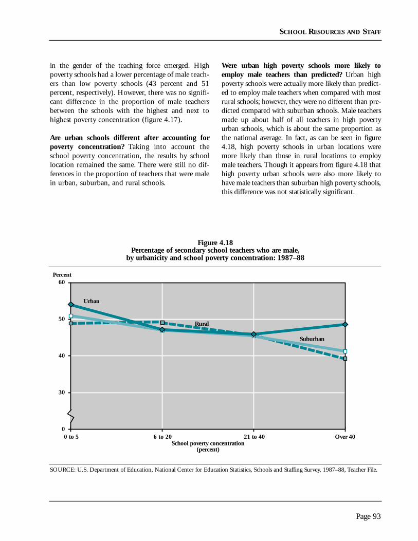
in the gender of the teaching force emerged. Highpoverty schools had a lower percentage of male teach-ers than low poverty schools (43 percent and 51percent, respectively). However, there was no signifi-cant difference in the proportion of male teachersbetween the schools with the highest and next tohighest poverty concentration (figure 4.17).
Are urban schools different after accounting forpoverty concentration? Taking into account theschool poverty concentration, the results by schoollocation remained the same. There were still no dif-ferences in the proportion of teachers that were malein urban, suburban, and rural schools.
Were urban high poverty schools more likely toemploy male teachers than predicted? Urban highpoverty schools were actually more likely than predict-ed to employ male teachers when compared with mostrural schools; however, they were no different than pre-dicted compared with suburban schools. Male teachersmade up about half of all teachers in high povertyurban schools, which is about the same proportion asthe national average. In fact, as can be seen in figure4.18, high poverty schools in urban locations weremore likely than those in rural locations to employmale teachers. Though it appears from figure 4.18 thathigh poverty urban schools were also more likely tohave male teachers than suburban high poverty schools,this difference was not statistically significant.
Page 93
SCHOOL RESOURCES AND STAFF
Figure 4.18Percentage of secondary school teachers who are male,
by urbanicity and school poverty concentration: 1987–88
Percent
0 to 5 6 to 20 21 to 40 Over 40
Suburban
Urban
Rural
0
30
40
50
60
School poverty concentration(percent)
SOURCE: U.S. Department of Education, National Center for Education Statistics, Schools and Staffing Survey, 1987–88, Teacher File.
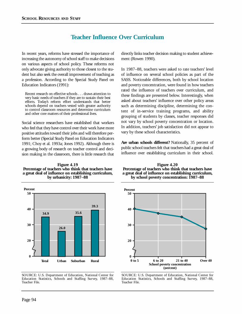
In recent years, reforms have stressed the importance ofincreasing the autonomy of school staff to make decisionson various aspects of school policy. These reforms notonly advocate giving authority to those closest to the stu-dent but also seek the overall improvement of teaching asa profession. According to the Special Study Panel onEducation Indicators (1991):
Recent research on effective schools . . . draws attention tovery basic needs of teachers if they are to sustain their bestefforts. Today’s reform effort understands that betterschools depend on teachers vested with greater authorityto control classroom resources and determine curriculumand other core matters of their professional lives.
Social science researchers have established that workerswho feel that they have control over their work have morepositive attitudes toward their jobs and will therefore per-form better (Special Study Panel on Education Indicators1991; Choy et al. 1993a; Jones 1992). Although there isa growing body of research on teacher control and deci-sion making in the classroom, there is little research that
directly links teacher decision making to student achieve-ment (Rowen 1990).
In 1987–88, teachers were asked to rate teachers’ levelof influence on several school policies as part of theSASS. Noticeable differences, both by school locationand poverty concentration, were found in how teachersrated the influence of teachers over curriculum, andthese findings are presented below. Interestingly, whenasked about teachers’ influence over other policy areassuch as determining discipline, determining the con-tent of in-service training programs, and abilitygrouping of students by classes, teacher responses didnot vary by school poverty concentration or location.In addition, teachers’ job satisfaction did not appear tovary by these school characteristics.
Are urban schools different? Nationally, 35 percent ofpublic school teachers felt that teachers had a great deal ofinfluence over establishing curriculum in their school.
Page 94
SCHOOL RESOURCES AND STAFF
Teacher Influence Over Curriculum
Percent
Total Urban Suburban Rural0
20
30
40
50
35.6
39.3
26.0
34.9
Percent
School poverty concentration(percent)
0 to 5 6 to 20 21 to 40 Over 400
20
30
40
50
Figure 4.19Percentage of teachers who think that teachers havea great deal of influence on establishing curriculum,
by urbanicity: 1987–88
Figure 4.20Percentage of teachers who think that teachers havea great deal of influence on establishing curriculum,
by school poverty concentration: 1987–88
SOURCE: U.S. Department of Education, National Center forEducation Statistics, Schools and Staffing Survey, 1987–88,Teacher File.
SOURCE: U.S. Department of Education, National Center forEducation Statistics, Schools and Staffing Survey, 1987–88,Teacher File.

When comparisons were made based on school location,however, urban teachers were less likely than suburban orrural teachers to feel that teachers had a great deal ofinfluence in this area. Twenty-six percent of urban teach-ers thought that teachers had a great deal of influenceover curriculum, as opposed to 36 percent of suburbanand 39 percent of rural teachers (figure 4.19).
Are high poverty schools different? Teachers’ per-ceived influence over curriculum tended to diminishas the concentration of poverty in their schoolsincreased. While 41 percent of teachers in low pover-ty schools reported that teachers had a great deal ofinfluence over curriculum, 28 percent of teachers inhigh poverty schools did so (figure 4.20).
Are urban schools different after accounting for povertyconcentration? School location still mattered after takinginto account differences in school poverty concentration.Teachers from schools in urban locations were still less
likely than teachers from suburban or rural schools tothink that teachers have a great deal of influence overestablishing curriculum when the concentration of pover-ty in their schools was held constant.
Were teachers in urban high poverty schools less likelyto have a great deal of influence over establishing cur-riculum than predicted? Teachers in urban high povertyschools were less likely to report that teachers have agreat deal of influence over curriculum than teachers inrural high poverty schools, but they reported a similarlevel of influence compared with teachers in suburbanhigh poverty schools (figure 4.21). Twenty-two percentof teachers in high poverty urban schools thought thatteachers had a great deal of influence over curriculum.However, it did not appear that teachers in urban highpoverty schools considered teachers to be less influen-tial than would be predicted based on the patterns forurban and high poverty schools separately.
Page 95
SCHOOL RESOURCES AND STAFF
Figure 4.21Percentage of teachers who think that teachers have a great deal of influence on establishing curriculum,
by urbanicity and school poverty concentration: 1987–88
Percent
0 to 5 6 to 20 21 to 40 Over 40
Suburban
Urban
Rural
0
20
30
40
50
School poverty concentration(percent)
SOURCE: U.S. Department of Education, National Center for Education Statistics, Schools and Staffing Survey, 1987–88, Teacher File.

Clearly, the consistent presence of the teacher in theclassroom is of paramount importance in providinginstruction to students. Beyond this, some research hassuggested that high staff absenteeism indicates poorworker morale. Is there evidence to suggest that teacherabsenteeism is a greater problem in urban schools, highpoverty schools, or both? Teacher ratings of the seri-ousness of the problem of teacher absenteeism in theirschool, drawn from the 1987–88 SASS, are reportedbelow.24
Are urban schools different? Nationally, 23 percent ofteachers viewed teacher absenteeism as a moderate toserious problem in their schools. When responses werecompared by the location of the school, urban teacherswere more likely than teachers in both suburban andrural schools to consider teacher absenteeism as a prob-lem. This can be clearly seen in figure 4.22, which
shows that approximately 31 percent of urban teachersreported their co-workers’ attendance as a moderate orserious problem, as compared with 23 percent of sub-urban and 20 percent of rural teachers.
Are high poverty schools different? A clear relationshipwas also found between school poverty concentrationand teachers’ perception of teacher absenteeism.Thirty-one percent of teachers in the high povertyschools reported that they considered teacher absen-teeism a problem, while 21 percent of teachers in thelow poverty schools reported similarly. In fact, whenthe teachers from the high poverty schools were com-pared with their peers from schools in the other threepoverty concentration categories, teachers from highpoverty schools were more likely to perceive teacherabsenteeism as a moderate to serious problem (figure4.23).
Page 96
SCHOOL RESOURCES AND STAFF
Teacher Absenteeism
Percent
Total Urban Suburban Rural0
10
20
30
40
23.4
19.6
23.4
30.6
Percent
School poverty concentration(percent)
0 to 5 6 to 20 21 to 40 Over 400
10
20
30
40
Figure 4.22Percentage of teachers who consider teacher
absenteeism a problem in their school, by urbanicity: 1987–88
Figure 4.23Percentage of teachers who consider teacher
absenteeism a problem in their school, by school poverty concentration: 1987–88
SOURCE: U.S. Department of Education, National Center forEducation Statistics, Schools and Staffing Survey, 1987–88,Teacher File.
SOURCE: U.S. Department of Education, National Center forEducation Statistics, Schools and Staffing Survey, 1987–88,Teacher File.

Are urban schools different after accounting forpoverty concentration? After taking into account vary-ing levels of poverty concentration, the responses ofteachers in urban schools were still higher than those ofteachers in suburban and rural schools.
Was teacher absenteeism more likely to be perceivedas a moderate to serious problem in urban high pover-ty schools than predicted? Teacher absenteeism wasperceived to be a problem by a similarly high percent-age of teachers in urban and suburban high povertyschools (37 and 35 percent, respectively), but was con-sidered a greater problem in urban than in rural high
poverty schools. However, the responses of teachers inurban high poverty schools were at predicted levels,given their school’s location and poverty concentration(figure 4.24).
Page 97
SCHOOL RESOURCES AND STAFF
24It is interesting to note that when asked the same question,administrators responded similarly but overall seemed to viewthe problem of teacher absenteeism as less serious. This is gener-ally true of all responses to opinion questions from the 1987–88SASS when comparisons were made between teachers andadministrators evaluating school problems. Although theresponses follow similar patterns by location and poverty con-centration in the school (that is, they are usually considered asmore serious problems in urban schools and in high povertyschools when compared to other school types), administratorsseem less likely to view problems as serious than do teachers.
Figure 4.24Percentage of teachers who consider teacher absenteeism a problem in their school,
by urbanicity and school poverty concentration: 1987–88
Percent
0 to 5 6 to 20 21 to 40 Over 40
Suburban
Urban
Rural
0
10
20
30
40
School poverty concentration(percent)
SOURCE: U.S. Department of Education, National Center for Education Statistics, Schools and Staffing Survey, 1987–88, Teacher File.

The programs and courses in which students participatecan influence their achievement in school, their oppor-tunities to learn, and their potential experiences aftergraduating from high school. This section explores stu-dent participation in selected public school programsand courses at three levels: preschool, elementary, andsecondary. Not all programs and courses could be pre-sented. Those that were selected had varying rates ofparticipation by school location and poverty concentra-tion, and bore important relationships to outcomes.
Many parents elect to send their children to preschooland kindergarten before the age of mandatory schooling.Previous research has suggested a strong relationshipbetween preschool attendance—in particular, high-quality, center-based early childhood programs—andlower participation rates in special education, lowerrates of grade retention through the high school years,and higher rates of high school completion and higherearnings in the labor force (Hofferth et al. 1994). Thissection documents differences in the preschool atten-dance rates of students in schools with varyingconcentrations of poverty and in different locations.
Public schools offer programs and services designed tomeet students’ special needs, such as bilingual educa-tion, English as a second language, remedial readingand mathematics, special education, gifted and talent-ed programs, day care, Chapter 1 (now Title 1) anddiagnostic services. The availability of these programs isclosely related to school size and level (whether a schoolis elementary or secondary) and each district’s policies(Choy et al. 1993b). As part of this study, an analysis ofthe availability of these programs was undertaken todetermine if program offerings varied by school loca-tion or level of poverty concentration. It was found thatmost programs were widely available. As a general rule,urban schools and high poverty schools were as likely tohave such programs as suburban schools. More oftenthan not, rural schools appeared less likely to offer awide range of programs than either urban or suburbanschools.
The availability of programs was often found to berelated to the nature of the needs addressed by the pro-grams. For example, Chapter 1 (Title 1) programsdirected at disadvantaged students were found to bemore prevalent in high poverty than low povertyschools in all locales. However, remedial reading andmathematics were found everywhere, as students need-ing these programs are found everywhere. Such obviouspatterns did not warrant further analysis. Gifted andtalented programs were selected for additional analysisbecause gifted and talented children are theoreticallyfound everywhere, but programs serving them are not.Therefore, data on the availability of gifted and talent-ed programs are presented in this section.
Consistent with the findings of chapter 2 and moregenerally with the findings of education researchers,one would expect students from high poverty schoolsand urban schools to be more likely to score lower onachievement tests overall and to need remedial pro-grams. Similarly, on average, students from highpoverty and urban schools would be less likely to berepresented in advanced courses, particularly in scienceand mathematics, and to be overrepresented in voca-tional courses. Patterns of coursetaking were examinedusing transcripts of high school seniors to determine ifthere were differences between groups of students intheir tendency to take vocational education oradvanced courses.
Findings
• Urban public school students attended preschoolat rates that fell between their suburban and ruralpeers; however, after accounting for the level ofpoverty in their schools, their preschool attendancerates differed only from rural students’ rates.Students from high poverty schools, regardless oflocation, were less likely to have attendedpreschool than students from schools with lowerpoverty concentrations. Rural students from allbut the low poverty schools were also found to be
Page 98
School Programs and Coursetaking

less likely to have attended preschool than studentsfrom urban and suburban schools.
• Urban public schools offered fewer gifted andtalented programs at the elementary school levelthan suburban schools, even after accounting fordifferences in school poverty concentration.
• Neither the likelihood of greater than averageparticipation in vocational education nor takinghigher level courses was found to be related to anurban setting apart from poverty concentration.When poverty was taken into account, urbanstudents took vocational education courses andhigher level mathematics at rates similar to thoseof their suburban and rural peers.
• High poverty urban public schools were as likelyto offer gifted and talented programs as highpoverty suburban schools, but were less likelythan predicted to offer these programs than ruralschools. Their students were more likely to haveattended preschool than those in high povertyrural, but not suburban schools.
• High poverty public schools, in general,offered gifted and talented programs less fre-quently than low poverty schools. Studentswere more likely to take vocational educationand were less likely to take more advancedcourses as the poverty level in their schoolincreased.
Page 99
SCHOOL PROGRAMS AND COURSETAKING

As stated above, research has suggested that preschoolattendance is related to later school success, particu-larly for students facing greater disadvantages(Hofferth et al. 1994). Given the importance ofpreschool and early childhood programs, were stu-dents across all locations and poverty concentrationsequally likely to have attended preschool? The answerto this question is obtained from the NationalEducation Longitudinal Study of 1988 (NELS:88),which asked parents of 8th graders to report whetheror not their child had attended preschool or nurseryschool programs. Since the students would haveattended preschool during the late 1970s, these datado not account for changes in preschool attendancethat have occurred since that time.
Are urban schools different? Nationally, according totheir parents, 51 percent of public school 8th gradersattended preschool, with urban students being less like-ly than suburban students and more likely than ruralstudents to have attended. Fifty-three percent of stu-dents attending urban schools in the 8th grade hadattended preschool compared with 58 percent of subur-ban and only 40 percent of rural students (figure 4.25).
Are high poverty schools different? Rates of preschoolattendance varied according to the poverty concentrationof the schools the 8th graders attended. Forty percent ofthe students attending the highest poverty schools hadattended preschool compared with 64 percent of studentsin the lowest poverty schools (figure 4.26).
Page 100
SCHOOL PROGRAMS AND COURSETAKING
Preschool Attendance
Percent
Total Urban Suburban Rural0
30
40
50
60
80
40.3
51.1 52.7
70
58.3
Percent
0
30
40
50
60
80
70
School poverty concentration(percent)
0 to 5 6 to 20 21 to 40 Over 40
Figure 4.25Percentage of 8th-grade students
who attended preschool, by urbanicity: 1988
Figure 4.26Percentage of 8th-grade students
who attended preschool, by school poverty concentration: 1988
SOURCE: U.S. Department of Education, National Center forEducation Statistics, National Education Longitudinal Study of1988, Base Year Parent File.
SOURCE: U.S. Department of Education, National Center forEducation Statistics, National Education Longitudinal Study of1988, Base Year Parent File.

Are urban schools different after accounting forpoverty concentration? After accounting for differ-ences in school poverty concentration across schoollocales, urban students were just as likely to haveattended preschool as suburban students, but were stillmore likely to have attended than rural students. Thatis, the higher poverty concentration in urban schoolsseems to account for the differences between studentsin urban and suburban schools, but not the differencebetween urban and rural students. Rural students wereless likely to have attended preschool than urban stu-dents at all levels of school poverty except the lowest.
Were students from urban high poverty schools lesslikely to have attended preschool than predicted?Urban students from schools with the highest pover-ty concentration were as likely as one would predictfrom the combination of their schools’ characteristicsto have attended preschool (figure 4.27). In fact, 45percent of the parents of students from urban schoolswith the highest poverty concentration reported thattheir children had attended preschool compared with34 percent of the parents of students attending highpoverty rural schools. Students in urban and subur-ban high poverty schools had about the same levels ofpreschool attendance.
Page 101
SCHOOL PROGRAMS AND COURSETAKING
Figure 4.27Percentage of 8th-grade students who attended preschool,
by urbanicity and school poverty concentration: 1988
Percent
0 to 5 6 to 20 21 to 40 Over 40
Suburban
Urban
Rural
0
30
40
60
70
80
School poverty concentration(percent)
50
SOURCE: U.S. Department of Education, National Center for Education Statistics, National Education Longitudinal Study of 1988, BaseYear Parent File.

SCHOOL PROGRAMS AND COURSETAKING
Gifted and talented programs provide those studentsselected by ability with the opportunity to expand theireducation beyond the basic curriculum. Some researchershave suggested that these programs are not available toall students equally, and that students in inner-city urbanpublic schools are particularly unlikely to be offered orplaced in programs for students of high ability (Oakes1990). If these reports are true, some students who couldbenefit from more challenging curriculum may beplaced at an unnecessary disadvantage when comparedwith other similar students. Comparisons of the avail-ability of gifted and talented programs between publicschools can be made using data from the 1987–88SASS. Elementary schools were chosen for this analysisbecause of the importance of early coursework in deter-mining later placement in academic tracks in secondaryschool, and the greater prevalence of these programs atthe elementary level.25
Are urban schools different? In 1987–88, 77 percentof public elementary schools offered gifted and tal-ented programs nationally. Urban elementaryschools, however, were less likely than suburbanschools to offer these programs (figure 4.28).Seventy-three percent of urban elementary schoolsoffered these programs compared with 84 percent ofsuburban schools. However, urban and rural schoolsdid not differ in the proportions offering gifted andtalented programs.
Are high poverty schools different? Schools withhigh poverty concentrations were less likely thanother schools to offer gifted and talented programs.Of schools with the highest poverty concentrations,70 percent reported offering a gifted and talentedprogram, while 78 to 83 percent of other schools didso (figure 4.29).
Page 102
Gifted and Talented Programs
Percent
Total Urban Suburban Rural0
50
60
70
80
100
84.1
75.576.7
73.2
90
Percent
0
50
60
70
80
100
90
School poverty concentration(percent)
0 to 5 6 to 20 21 to 40 Over 40
Figure 4.28Percentage of elementary schools that offer
gifted and talented programs, by urbanicity: 1987–88
Figure 4.29Percentage of elementary schools that offer
gifted and talented programs, by school poverty concentration: 1987–88
SOURCE: U.S. Department of Education, National Center forEducation Statistics, Schools and Staffing Survey, 1987–88,School File.
SOURCE: U.S. Department of Education, National Center forEducation Statistics, Schools and Staffing Survey, 1987–88,School File.

Are urban schools different after accounting forpoverty concentration? After accounting for schoolpoverty concentration, the differences between urbanand suburban schools remained. That is, the higherpoverty concentration of urban schools was not theonly explanation for the disparity in the rate at whichgifted and talented programs were offered in urban andsuburban schools.
Were urban high poverty schools less likely to offer gift-ed and talented programs than predicted? Students inhigh poverty urban schools are at a disadvantage relativeto rural schools in that they are less likely than predictedto have gifted and talented programs in their school.High poverty urban schools offered gifted and talentedprograms at a lower rate than rural high poverty schools
(figure 4.30). Sixty-six percent of urban high povertyschools offered gifted and talented programs comparedwith just over 70 percent of rural high poverty schools.Suburban high poverty schools were just as likely as urbanhigh poverty schools to offer these programs; however,urban students at schools with the lowest poverty con-centration are at a relative disadvantage compared withsuburban schools. At the 0–5 percent level of povertyconcentration, 80 percent of urban schools had giftedand talented programs compared with 94 percent of sub-urban schools. The percentages were similar for suburbanand urban schools with higher poverty concentrations.
Page 103
SCHOOL PROGRAMS AND COURSETAKING
Figure 4.30Percentage of elementary schools that offer gifted and talented programs,
by urbanicity and school poverty concentration: 1987–88
Percent
0 to 5 6 to 20 21 to 40 Over 40
Suburban
Urban
Rural
0
50
60
80
90
100
School poverty concentration(percent)
70
SOURCE: U.S. Department of Education, National Center for Education Statistics, Schools and Staffing Survey, 1987–88, School File.
25The definition of elementary covers schools that includegrades from kindergarten through the 6th grade, or ungraded,with no grades higher than the 8th.

Nearly all students take a vocational course duringtheir high school career. However, some students takeconsiderably more vocational education courses thanothers. In this analysis, students who take six or morecredits of vocational education are considered to beparticipating in vocational education more than theaverage high school student (Tuma 1995). The fol-lowing analysis presents data from the high schooltranscripts of seniors obtained as part of the 1990National Assessment of Educational Progress (NAEP)showing that vocational coursetaking varies by schoollocation and poverty concentration. Interestingly, asimilar analysis of the total number of academic cred-its students took did not reveal similar variation bythese two school characteristics. This indicates that,although on average some groups of students takemore vocational courses than others, academic
coursetaking does not vary when analyzed at theschool level. However, research suggests that studentswho participate more in vocational education coursesmay take fewer advanced academic courses than theirpeers (Tuma 1996).
Are urban schools different? In 1990, about 19 percentof all graduating public high school seniors had takensix or more credits in vocational education (figure4.31).26 Although it appears that urban students weremore likely to take vocational education courses (20percent) than suburban students (14 percent) and lesslikely than rural students (25 percent), these differencesare not statistically significant. Students in urbanschools were just as likely to take six or more credits invocational education than students in suburban orrural schools. Rural students, however, were more
Page 104
SCHOOL PROGRAMS AND COURSETAKING
Vocational Coursetaking
Percent
Total Urban Suburban Rural0
10
20
25
30
13.6
24.7
19.918.6
15
Percent
School poverty concentration(percent)
0 to 5 6 to 20 21 to 40 Over 400
10
20
25
30
15
Figure 4.31Percentage of graduating high school seniors who
took 6 or more credits in vocational education,by urbanicity: 1990
Figure 4.32Percentage of graduating high school seniors who
took 6 or more credits in vocational education,by school poverty concentration: 1990
SOURCE: U.S. Department of Education, National Center forEducation Statistics, National Assessment of EducationalProgress, 1990 High School Transcript Study.
SOURCE: U.S. Department of Education, National Center forEducation Statistics, National Assessment of EducationalProgress, 1990 High School Transcript Study.

likely than suburban students to take six or morecredits of vocational education—about one-fourth ofrural students took that many credits compared withsuburban students.
Are high poverty schools different? Students in publicschools with high poverty concentrations were morelikely to take six or more vocational credits than stu-dents in low poverty schools (figure 4.32). In the highpoverty schools, one-fourth of all graduating seniorshad completed six or more credits in vocational educa-tion compared with 15 percent of students in the lowpoverty schools.27
Are urban schools different after accounting forpoverty concentration? After accounting for differ-ences in school poverty concentration, urban studentswere still not statistically different in their vocationalcoursetaking than other students; however, rural stu-dents were, again, more likely than suburban studentsto take six or more vocational education credits.
Were students in urban high poverty schools morelikely to have taken six or more vocational creditsthan predicted? Students in high poverty urban pub-lic schools were about as likely to take six or morevocational education credits as one would predictgiven the location and poverty concentration of theirschools. That is, being in a high poverty urban schoolwas not related to a greater than predicted incidenceof taking a lot of vocational courses.28
Page 105
SCHOOL PROGRAMS AND COURSETAKING
26One credit (or Carnegie Unit) is defined as a 1-year course meeting1 hour a day.
27The categories of poverty concentration used in this section are forillustrative purposes only. The actual statistical test was conducted ona continuous poverty concentration variable. Since the sample sizesfor schools by urbanicity and poverty concentration combined weretoo small to produce reliable estimates, no comparisons were madebetween urban high poverty and other high poverty schools.
28No third figure is presented since the sample sizes for schools byurbanicity and poverty concentration are too small to produce reliableestimates.

A key feature of what constitutes a quality educationis the opportunity to take advanced course work.Ideally, a measure of differences in course offeringsacross school types is desired, since if courses are notoffered, students are not able to take them, and dif-ferences between schools in student achievement andattainment can result when students are not exposedto the same curricula. However, information oncourse offerings that schools provide is not a reliablepredictor of what classes are actually offered during aschool year. Student coursetaking is the best measureavailable, even though differences in coursetakingreflect students’ placement and course selection inaddition to differences in course offerings. Further, itis not known precisely how consistently course titles
reflect similar content; however, limited evidencesuggests that course titles are reasonably reliable indi-cators of comparative content (Porter 1994).
The data source for this analysis is the high school tran-scripts of seniors in the 1990 National Assessment ofEducational Progress (NAEP). Since patterns ofadvanced coursetaking were found to be similar inmathematics, science, and foreign languages, only theresults of the analysis of geometry are presented.Geometry was the course chosen because it is the mostadvanced, yet least specialized, mathematics class that iswidely available and that a majority of students take.Also, evidence has shown that successful completion ofgeometry is related to a greater chance that students
Page 106
SCHOOL PROGRAMS AND COURSETAKING
Mathematics Coursetaking
Percent
Total Urban Suburban Rural0
50
60
70
80
72.8
66.2
57.4
67.8
Percent
School poverty concentration(percent)
0 to 5 6 to 20 21 to 40 Over 400
50
60
70
80
Figure 4.33Percentage of graduating high school
seniors who took geometry,by urbanicity: 1990
Figure 4.34Percentage of graduating high school
seniors who took geometry,by school poverty concentration: 1990
SOURCE: U.S. Department of Education, National Center forEducation Statistics, National Assessment of EducationalProgress, 1990 High School Transcript Study.
SOURCE: U.S. Department of Education, National Center forEducation Statistics, National Assessment of EducationalProgress, 1990 High School Transcript Study.

will go on to college when compared with their peerswho complete only algebra (Pelavin and Kane 1990).
Are urban schools different? In 1990, a little morethan two-thirds (68 percent) of graduating publicschool seniors had taken geometry in high school(figure 4.33). Urban students were less likely thansuburban students to have taken geometry. Fifty-seven percent of urban students had credits in geometrycompared with almost 73 percent of suburban students.However, urban and rural students were not statisticallydifferent from each other on this measure.
Are high poverty schools different? Students inschools with higher poverty concentrations were lesslikely to have taken geometry than other students(figure 4.34). Sixty percent of students in the highpoverty schools had taken geometry compared with74 percent of students in the lowest poverty schools.29
Are urban schools different after accounting forpoverty concentration? When the school poverty
concentration was taken into account, the differencebetween the proportion of urban and suburban studentstaking geometry was no longer statistically significant.Rural and suburban students were just as likely tohave taken geometry as were urban students.30
Were students in urban high poverty schools less like-ly to have taken geometry than predicted? Students inurban high poverty schools were just as likely to havetaken geometry as predicted from the combination ofthe effects of an urban and high poverty setting. Therewas no evidence that they were at any additional disad-vantage related to the interaction, or compoundingeffect, of the two.
Page 107
SCHOOL PROGRAMS AND COURSETAKING
29The categories of poverty concentration used in this section are forillustrative purposes only. The actual statistical test was conducted ona continuous poverty concentration variable.
30No third figure is presented since the sample sizes for schools byurbanicity and poverty concentration are too small to produce reliableestimates.

Recently, researchers and policymakers have focusedattention on the importance of the school learningenvironment and the influence of individual and peerbehaviors on student performance. Goal six of theNational Education Goals states that by the year2000, “every school in America will be free of drugsand violence and will offer a disciplined environmentconducive to learning” (National Education GoalsPanel 1992). Because learning is constrained in anatmosphere of fear or disorderliness, student behaviorinfluences school atmosphere and the climate forlearning—whether it takes the form of violence andrisk-taking activities (such as bringing a weapon toschool or using alcohol) or a low commitment to aca-demic effort (such as poor attendance, discipline, orstudy habits). These student behaviors also play a keyrole in determining student success in school andbeyond. Studies of students considered to be “at risk”for school failure have shown that these students arelikely to complete less homework, attend school lessfrequently, exhibit more aggressive behavior, and useillicit drugs more than their peers who are not at risk(Kaufman and Bradby 1992).
The indicators presented in this section can bebroadly grouped into four categories of studentbehavior. Two indicators of student academic effortare time spent doing homework and watching televi-sion. The amount and quality of time spent in theclassroom is represented by student absenteeism andtime spent on discipline in the classroom. School vio-lence is measured by how safe students feel in schooland the extent of weapons possession at school.Finally, data on two student risk-taking behaviors,student alcohol use and pregnancy, are presented.Given the nature of these problems, the analysis islimited to secondary school data, with the exceptionof 8th-grade teacher reports of time spent maintain-ing classroom order and discipline.
When considering the results, it is important toemphasize that the actual incidence of a particularstudent behavior cannot be extrapolated from thedata. These data reflect teachers’ and students’ percep-tions of a particular problem. In one sense, teacher andstudent perceptions are direct measures of classroomand school conditions. However, teachers may havedifferent perceptions of the seriousness of studentbehavior problems regardless of the frequency withwhich students engage in these particular behaviors intheir schools. Behavior that might be consideredintolerable to a teacher in one school may be a morecommon occurrence and, thus, less problematic to ateacher in another.
Findings
• About half of the student behaviors studiedwere more likely to be worse in public urbanschools than in suburban or rural schools, evenafter accounting for the higher concentrationof poverty in urban schools. More time wasspent maintaining classroom discipline inurban schools, and student absenteeism, pos-session of weapons, and student pregnancywere greater problems.
• For the other half of behaviors studied, urbanstudents were similar to other students afteraccounting for poverty differences. They spentthe same amount of time doing homework andwatching television as other students.Although they felt less safe at school than ruralstudents, they were as likely to report feelingsafe as suburban students. Urban students wereconsidered by their teachers to be as likely touse alcohol as suburban students, but less likelythan rural students.
Page 108
Student Behavior

• Discipline was more likely to be a problem inurban high poverty schools than in any otherhigh poverty schools. Student absenteeism andweapons possession were worse in urban thanin rural high poverty schools, but were thesame as in suburban schools with a similarpoverty concentration.
• Students in urban high poverty schools weresimilar to students in other high poverty schools
in their homework effort, feelings of safety,alcohol use, and problems with pregnancy.
• The hours that students in urban high povertyschools spent watching television were higherthan predicted, and cannot be explained by thecombination of an urban school location andhigh poverty concentration alone.
Page 109
STUDENT BEHAVIOR

Time spent watching television limits the number ofhours a student has available to complete homework(Mullis et al. 1991). Moreover, spending large amountsof time watching television has been correlated withweaker academic performance in recent national assess-ments (U.S. Department of Education 1993b). TheNational Assessment of Educational Progress (NAEP)has documented that students watched more hours oftelevision and spent less time on homework per day in1990 than in 1982 (U.S. Department of Education1993b).
Are urban schools different? Nationally, 33 percent ofpublic school 10th graders in 1990 reported watchingat least 3 hours of television on weekdays. Urban stu-dents (37 percent) were more likely than suburbanstudents (30 percent) to watch this much television.
However, there was no statistical difference betweenurban and rural students (35 percent) on this measure(figure 4.35).
Are high poverty schools different? Students whoattend high poverty schools were more likely to watch3 or more hours of television per weekday than theirpeers in schools with lower poverty concentrations.Forty-three percent of students in high poverty schoolswatched 3 or more hours of television compared with26 percent of students in low poverty schools, a differ-ence of 17 percentage points (figure 4.36).
Are urban schools different after accounting forpoverty concentration? After accounting for schoolpoverty concentration, the difference between studentsattending urban and suburban schools disappeared.
Page 110
STUDENT BEHAVIOR
Hours of Television Watched on Weekdays
Percent
Total Urban Suburban Rural0
20
30
40
50
29.6
35.436.7
33.2
Percent
School poverty concentration(percent)
0 to 5 6 to 20 21 to 40 Over 400
20
30
40
50
Figure 4.35Percentage of 10th-grade students who watch 3 or more hours of television on weekdays,
by urbanicity: 1990
Figure 4.36Percentage of 10th-grade students who watch 3 or more hours of television on weekdays,
by school poverty concentration: 1990
SOURCE: U.S. Department of Education, National Center forEducation Statistics, National Education Longitudinal Study of1988, First Follow-up Student File.
SOURCE: U.S. Department of Education, National Center forEducation Statistics, National Education Longitudinal Study of1988, First Follow-up Student File.

Therefore, the greater percentage of urban studentswatching a lot of television compared with their sub-urban counterparts can be explained by the greaterlikelihood that urban students attend schools withhigher poverty concentrations.
Were students in urban high poverty schools likely toview television more frequently than predicted? Nearlyone-half of students in urban high poverty schoolsreported watching television more than 3 hours per day.In fact, the rate for urban high poverty schools was high-er than predicted given the overall rates of television
watching for urban students and students in all schoolswith high poverty concentrations. Although on average,after accounting for poverty, the proportion of urbanstudents watching a lot of television was no differentfrom suburban and rural students, this average masks thedifferences by level of poverty within urban schools.There was a wider gap between the television viewinghabits of urban students in high poverty schools com-pared with urban students in low poverty schools thanthere was for either suburban or rural students (figure4.37). In other words, poverty concentration matteredmore in urban schools than in schools in other locations.
Page 111
STUDENT BEHAVIOR
Figure 4.37Percentage of 10th-grade students who watch 3 or more hours of television on weekdays,
by urbanicity and school poverty concentration: 1990
Percent
0 to 5 6 to 20 21 to 40 Over 40
Suburban
Urban
Rural
0
20
30
40
50
School poverty concentration(percent)
SOURCE: U.S. Department of Education, National Center for Education Statistics, National Education Longitudinal Study of 1988, FirstFollow-up Student File.

The amount of time spent on homework is an impor-tant indicator of student effort. Tenth-grade studentsparticipating in the 1990 follow-up to the NELS:88survey were questioned about the amount of time theyspent on homework both in and out of school,31 andthese data are presented below.
Are urban schools different? No difference was foundin the number of hours students attending publicschools in different locations spent doing homework.The average number of hours that urban, suburban,and rural students spent on homework was a little over7 hours per week (figure 4.38).
Are high poverty schools different? The number ofhours of homework completed by students differedaccording to the poverty concentration of their schools.Students attending high poverty schools completed 6and a half hours of homework on average during theweek, while students in low poverty schools completedalmost 8 hours (figure 4.39).
Are urban schools different after accounting forpoverty concentration? There were still no differencesbetween students attending urban, suburban, and ruralschools after accounting for the varying school povertyconcentration.
Page 112
STUDENT BEHAVIOR
Hours Spent on Homework
Total Urban Suburban Rural0
6
7
8
9
7.47.37.4 7.4
Number of hours
School poverty concentration(percent)
0 to 5 6 to 20 21 to 40 Over 400
6
7
8
9Number of hours
Figure 4.38Average number of hours 10th-grade students
spend on homework per week, by urbanicity: 1990
Figure 4.39Average number of hours 10th-grade students
spend on homework per week,by school poverty concentration: 1990
SOURCE: U.S. Department of Education, National Center forEducation Statistics, National Education Longitudinal Study of1988, First Follow-up Student File.
SOURCE: U.S. Department of Education, National Center forEducation Statistics, National Education Longitudinal Study of1988, First Follow-up Student File.

Were students in urban high poverty schools lesslikely to spend time on homework than predicted?Students from urban high poverty schools did notspend less time doing homework than predicted. Infact, students attending these schools did as muchhomework as students in schools in other locationswith similar poverty concentrations. Thus, despitetheir unusually high rate of television watching, thesestudents did not appear to spend less time on home-
work than students in other high poverty schools(figure 4.40).
Page 113
STUDENT BEHAVIOR
31To create a figure for homework hours completed during the week,data on time spent on homework both in and out of school werecombined. In order to combine these data, which were already in dis-crete categories, a score midway between the range for each categorywas created; then, an overall score was created by summing the twoseparate scores for homework completed in and out of school. Theanalysis was conducted using this overall score.
Figure 4.40Average number of hours 10th-grade students spend on homework per week,
by urbanicity and school poverty concentration: 1990
Number of hours
0 to 5 6 to 20 21 to 40 Over 40
Suburban
Urban
Rural
0
6
7
8
9
School poverty concentration(percent)
SOURCE: U.S. Department of Education, National Center for Education Statistics, National Education Longitudinal Study of 1988, FirstFollow-up Student File.
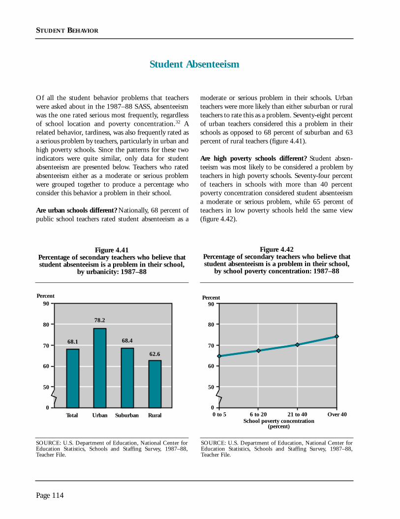
Of all the student behavior problems that teacherswere asked about in the 1987–88 SASS, absenteeismwas the one rated serious most frequently, regardlessof school location and poverty concentration.32 Arelated behavior, tardiness, was also frequently rated asa serious problem by teachers, particularly in urban andhigh poverty schools. Since the patterns for these twoindicators were quite similar, only data for studentabsenteeism are presented below. Teachers who ratedabsenteeism either as a moderate or serious problemwere grouped together to produce a percentage whoconsider this behavior a problem in their school.
Are urban schools different? Nationally, 68 percent ofpublic school teachers rated student absenteeism as a
moderate or serious problem in their schools. Urbanteachers were more likely than either suburban or ruralteachers to rate this as a problem. Seventy-eight percentof urban teachers considered this a problem in theirschools as opposed to 68 percent of suburban and 63percent of rural teachers (figure 4.41).
Are high poverty schools different? Student absen-teeism was most likely to be considered a problem byteachers in high poverty schools. Seventy-four percentof teachers in schools with more than 40 percentpoverty concentration considered student absenteeisma moderate or serious problem, while 65 percent ofteachers in low poverty schools held the same view(figure 4.42).
Page 114
STUDENT BEHAVIOR
Student Absenteeism
Percent
Total Urban Suburban Rural0
50
60
70
80
90
68.4
62.6
68.1
78.2
Percent
0
50
60
70
80
90
School poverty concentration(percent)
0 to 5 6 to 20 21 to 40 Over 40
Figure 4.41Percentage of secondary teachers who believe thatstudent absenteeism is a problem in their school,
by urbanicity: 1987–88
Figure 4.42Percentage of secondary teachers who believe thatstudent absenteeism is a problem in their school,
by school poverty concentration: 1987–88
SOURCE: U.S. Department of Education, National Center forEducation Statistics, Schools and Staffing Survey, 1987–88,Teacher File.
SOURCE: U.S. Department of Education, National Center forEducation Statistics, Schools and Staffing Survey, 1987–88,Teacher File.

Are urban schools different after accounting forpoverty concentration? Accounting for poverty con-centration did not eliminate the differences by schoollocation. Urban teachers were still more likely to consid-er student absenteeism a moderate or serious problemin their schools when compared with suburban andrural teachers.
Were teachers in urban high poverty schools morelikely to consider student absenteeism a problem intheir schools than predicted? Teachers in urban highpoverty schools were more likely to consider studentabsenteeism a problem than teachers in rural highpoverty schools (84 percent compared with 65 per-cent). However, this rate was no higher than predicted.
There was little difference between teachers in suburbanschools with moderately high to the highest povertyconcentrations and their urban counterparts on thismeasure. Teachers in urban and suburban schools weremore likely to consider student absenteeism a problemas school poverty concentration increased. However,the percentage of rural teachers rating student absen-teeism a problem was lower than that of teachers insuburban and urban schools, and it did not increase asmuch with poverty concentration as it did in urban andsuburban schools (figure 4.43).
Page 115
STUDENT BEHAVIOR
32Administrators also rated this as a serious problem most fre-quently.
Figure 4.43Percentage of secondary teachers who believe that student absenteeism is a problem in their school,
by urbanicity and school poverty concentration: 1987–88
Percent
0 to 5 6 to 20 21 to 40 Over 40
Suburban
Urban
Rural
0
50
60
70
80
90
School poverty concentration(percent)
SOURCE: U.S. Department of Education, National Center for Education Statistics, Schools and Staffing Survey, 1987–88, Teacher File.

Recent studies comparing U.S. and Asian classroom prac-tices have suggested that in the United States, teachersspend a greater proportion of time on activities otherthan instruction than they do in Japan and China(Stevenson and Stigler 1992). According to HaroldStevenson, American teachers spend proportionatelymore time disciplining students in the classroom thantheir Asian peers. Time spent on discipline means lesstime available for instruction and learning.
One index of need for discipline is the degree to whichAmerican children engage in irrelevant activities in theclassroom . . . Such activities as talking to other childrenand wandering about the classroom diminish the child’sown opportunities for learning and are potentially disrup-tive to other children. This type of irrelevant behavior, inaddition to the fidgeting and inattentiveness oftendescribed by American teachers, makes maintainingdiscipline a pervasive and difficult problem in Americanclassrooms (Stevenson and Stigler 1992).
Researchers have also suggested that teachers spend moretime disciplining students and maintaining order inschools in poor urban settings than in non-urban and
more advantaged schools (Karweit 1992). In this section,data from the base year of the National EducationLongitudinal Survey of 1988 (NELS:88) is used to exam-ine this perception. In NELS:88, 8th-grade teachers wereasked about the time they spent maintaining order anddiscipline in their classrooms.33 Less than 2 percent ofthese teachers reported that their classes met more than 5hours per week. Therefore, teachers who spent 1 hour ormore per week maintaining classroom order were spend-ing at least one-fifth of their instruction time on discipline.
Are urban schools different? Teachers of 8th-gradestudents in urban public schools were more likely tospend substantial amounts of time maintaining class-room order and discipline than their suburban andrural counterparts. Urban 8th-grade teachers werealmost twice as likely as rural teachers to report thatthey spend at least 1 hour per week maintaining orderin their classes (25 percent compared with 13 percent).Sixteen percent of suburban teachers reported spendingthis much classroom time on these tasks (figure 4.44).
Page 116
STUDENT BEHAVIOR
Time Spent Maintaining Classroom Discipline
Percent
Total Urban Suburban Rural0
10
20
30
40
16.4
12.6
24.6
16.7
Percent
School poverty concentration(percent)
0 to 5 6 to 20 21 to 40 Over 400
10
20
30
40
Figure 4.44Percentage of teachers of 8th-grade students
who spend at least 1 hour per week maintaining classroom order and discipline,
by urbanicity: 1988
Figure 4.45Percentage of teachers of 8th-grade students
who spend at least 1 hour per week maintaining classroom order and discipline,
by school poverty concentration: 1988
SOURCE: U.S. Department of Education, National Center forEducation Statistics, National Education Longitudinal Study of1988, Base Year Teacher File.
SOURCE: U.S. Department of Education, National Center forEducation Statistics, National Education Longitudinal Study of1988, Base Year Teacher File.

Are high poverty schools different? Teachers of 8th-grade students from the highest poverty schools weregenerally more likely to spend classroom time main-taining order and discipline than were teachers fromschools with lower poverty concentrations (figure4.45). In particular, 21 percent of 8th-grade teachersfrom high poverty schools spent at least 1 hour perweek in their classes on discipline compared with 12percent of teachers in low poverty schools.
Are urban schools different after accounting forpoverty concentration? After taking poverty concentra-tion into account, urban teachers of 8th-grade studentswere still more likely to spend at least 1 hour per weekmaintaining order in their classrooms. The higher pro-portion of poor students in urban locations is not theonly explanation for the fact that teachers in urbanschools were likely to spend more time discipliningtheir students than teachers in rural and suburbanschools.
Were teachers in urban high poverty schools more like-ly to spend at least 1 hour on discipline in theirclassrooms than predicted? Teachers of 8th-grade stu-
dents in urban high poverty schools were more likely tospend at least 1 hour maintaining classroom order anddiscipline than 8th-grade teachers in other high povertyschools. However, their responses were no different fromteachers in other urban schools with moderate levels ofpoverty concentration (figure 4.46). Twenty-eight per-cent of urban 8th-grade teachers spent this amount oftime on discipline—at least 10 percentage points higherthan 8th-grade teachers in suburban or rural high pover-ty schools. However, teachers in urban high povertyschools did not spend more time disciplining studentsthan predicted compared with teachers in other schools.This suggests that high poverty concentration and anurban setting do not interact to add to the already largeramounts of time teachers spend on maintaining disci-pline in these schools.
Page 117
STUDENT BEHAVIOR
33Although the student sample in the NELS:88 survey wasdesigned to represent the student population in the UnitedStates, the teacher sample is not nationally representative. Thismeans that one can discuss these data nationally for students, butnot teachers. In one of the following combinations of subjectareas—math and English, math and social studies, science andEnglish, or science and social studies—two teachers were chosenfor each student. (If one teacher taught both subjects to a stu-dent, then one teacher was chosen for that student.)
Figure 4.46Percentage of teachers of 8th-grade students who spend at least 1 hour per week maintaining
classroom order and discipline, by urbanicity and school poverty concentration: 1988
Percent
0 to 5 6 to 20 21 to 40 Over 40
Suburban
Urban
Rural
0
10
20
30
40
School poverty concentration(percent)
SOURCE: U.S. Department of Education, National Center for Education Statistics, National Education Longitudinal Study of 1988,Base Year Teacher File.

Perhaps no other school climate issue has received asmuch recent media attention as safety in the publicschools. Reports surface almost weekly on incidents ofweapons possession, drug use, violence, racial conflictand crime on school campuses, particularly in the innercities. There have even been individual reports of stu-dents choosing not to attend their classes out of fear.(Such behavior clearly may exacerbate the problem ofstudent absenteeism discussed earlier in this section.)34
Despite what appears to be increasing reports of schoolviolence, a recent study comparing sophomores in1980 and 1990 revealed that in 1990, 10th graderswere in general less likely to report that they felt unsafeat school than were students surveyed in 1980(Rasinski et al. 1993). Whether this suggests a positivechange in school safety nationally or simply increaseddesensitization to violence is unclear. Nevertheless, in
1990 the percentage of students who reported feelingunsafe at school differed by school location and povertyconcentration, as presented below.
Are urban schools different? Nationally, approximate-ly 9 percent of 10th graders agreed or strongly agreedthat they did not feel safe at school in 1990. Tenthgraders attending urban schools were more likely toreport that they did not feel safe at school—13 percentcompared with 8 percent each of suburban and ruralstudents (figure 4.47).
Are high poverty schools different? Students in highpoverty schools were less likely to feel safe than those inschools with the lowest poverty concentrations (figure4.48). However, students in schools with the highestpoverty concentration were just as likely to feel unsafe
Page 118
STUDENT BEHAVIOR
School Safety
Percent
Total Urban Suburban Rural0
5
10
20
7.8 7.58.8
12.615
Percent
School poverty concentration(percent)
0 to 5 6 to 20 21 to 40 Over 400
5
10
20
15
Figure 4.47Percentage of 10th-grade students who
do not feel safe at school, by urbanicity: 1990
Figure 4.48Percentage of 10th-grade students who
do not feel safe at school, by school poverty concentration: 1990
SOURCE: U.S. Department of Education, National Center forEducation Statistics, National Education Longitudinal Study of1988, First Follow-up Student File.
SOURCE: U.S. Department of Education, National Center forEducation Statistics, National Education Longitudinal Study of1988, First Follow-up Student File.

as those in schools with the next to highest concentra-tion of poverty. Approximately 12 percent of studentsin high poverty schools felt unsafe, compared with 6 to8 percent in schools with the lowest and next to lowestpoverty concentrations.
Are urban schools different after accounting forpoverty concentration? Once the higher poverty con-centrations in urban schools are considered, urban andsuburban students’ perception of school safety are sim-ilar; but urban students overall still felt less safe thantheir rural peers.
Were students in urban high poverty schools more like-ly to feel unsafe at school than predicted? Students inurban high poverty schools were just as likely to feelunsafe as students in high poverty schools in other loca-tions. In fact, the percentage who did not feel safe in
urban high poverty schools was not statistically differentfrom the percentages in other urban schools, with theexception of urban students in the lowest poverty schools.Thus, an urban high poverty setting did not present anyadditional safety risk from the students’ perspective.Given the heightened news reports, what seems most sur-prising is that the magnitude of the problem as reportedby students is not high, ranging from 5 percent of stu-dents in low poverty rural schools to approximately 16percent of students in urban and suburban schools witha poverty concentration of 21 to 40 percent (figure 4.49).
Page 119
STUDENT BEHAVIOR
34See, for example, The New York Times, October 15, 1993, B3.According to Robert D. McFadden, “20% of New York CityPublic-School Students Carry Weapons, Study Finds.” This state-ment refers to a study conducted in June 1992 by the FederalCenters for Disease Control and Prevention, the city HealthDepartment, and city school officials, which links school violenceto student attitudes.
Figure 4.49Percentage of 10th-grade students who do not feel safe at school,
by urbanicity and school poverty concentration: 1990
Percent
0 to 5 6 to 20 21 to 40 Over 40
Suburban
Urban
Rural
0
5
10
20
School poverty concentration(percent)
15
SOURCE: U.S. Department of Education, National Center for Education Statistics, National Education Longitudinal Study of 1988, FirstFollow-up Student File.

The presence of weapons on school campuses poses aserious threat to the school learning environment.Though still rare, shootings and weapon-related violentacts occurring inside or near schools have receivedmuch publicity in recent years, and, to the extent theydo occur, they interfere with the ability of students andteachers to concentrate on schooling.
Are urban schools different? Nationally, 11 percent ofteachers reported that weapons possession by studentswas a moderate or serious problem in their school in1987–88. Teachers’ responses, however, varied widelyby location (figure 4.50). Urban teachers were more
than twice as likely as suburban or rural teachers toview weapons possession as a problem in their schools—21 percent compared with 9 percent and 7 percent,respectively. This finding supports the perception thaturban students are exposed to more weapons in theschool than either suburban or rural students.
Are high poverty schools different? Teachers in highpoverty schools were more than twice as likely toreport that weapons possession was a problem thanteachers in schools with the two lowest concentra-tions of poverty (figure 4.51). Twenty-one percent ofteachers in high poverty schools reported that
Page 120
STUDENT BEHAVIOR
Student Possession of Weapons
Percent
Total Urban Suburban Rural0
10
20
30
40
9.16.8
11.1
21.3
Percent
School poverty concentration(percent)
0 to 5 6 to 20 21 to 40 Over 400
10
20
30
40
Figure 4.50Percentage of secondary teachers who believe that
student weapons possession is a problem in their school, by urbanicity: 1987–88
Figure 4.51Percentage of secondary teachers who believe thatstudent weapons possession is a problem in theirschool, by school poverty concentration: 1987–88
SOURCE: U.S. Department of Education, National Center forEducation Statistics, Schools and Staffing Survey, 1987–88,Teacher File.
SOURCE: U.S. Department of Education, National Center forEducation Statistics, Schools and Staffing Survey, 1987–88,Teacher File.

weapons possession was a problem compared with 6percent of teachers in the lowest poverty schools and10 percent of the teachers in schools with a 6–20 per-cent poverty concentration.
Are urban schools different after accounting for pover-ty concentration? After accounting for differences inschool poverty concentration, school location was stillfound to be strongly related to teacher responses.Teachers in urban schools were more likely to view stu-dent weapons possession as a problem in their schoolswhen compared with either suburban or rural teachers.
Were teachers in urban high poverty schools morelikely to view student possession of weapons as amoderate to serious problem in their schools thanpredicted? Teachers in urban high poverty schools weremore likely to report that weapons possession was aproblem than teachers in many other school types, buttheir reports were no different from teachers in urbanschools with the next highest poverty concentrationand suburban schools with the highest poverty concen-trations. The combination of an urban and a highpoverty setting did not reveal an additional risk ofexposure to weapons (figure 4.52).
Page 121
STUDENT BEHAVIOR
Figure 4.52Percentage of secondary teachers who believe that student weapons possession is a problem in their
school, by urbanicity and school poverty concentration: 1987–88
Percent
0 to 5 6 to 20 21 to 40 Over 40
Suburban
Urban
Rural
0
10
20
30
40
School poverty concentration(percent)
SOURCE: U.S. Department of Education, National Center for Education Statistics, Schools and Staffing Survey, 1987–88, Teacher File.

Some recent reports on the “at-risk” behaviors of youthhave shown that student use of illegal substances hasdeclined over the past two decades (U.S. Departmentof Education 1993c). Nevertheless, students’ use ofalcohol and drugs has remained a serious issue for edu-cators and parents, with recent reports indicating thatthe use of illegal substances by teenagers may be againon the rise (University of Michigan 1994). Even in thelate 1980s, alcohol use among students seems to havebeen of particular concern to teachers who participatedin the 1987–88 SASS. Secondary school teachersnationwide rated student use of alcohol as a moderateor serious problem in their schools more frequentlythan student drug abuse (63 percent compared with 57percent).
Are urban schools different? Nationwide, 63 percent ofteachers considered student alcohol use as a moderate toserious problem in their schools. Teachers in urbanschools were less likely (58 percent) to consider alcoholuse a problem than were teachers from either suburban(63 percent) or rural (65 percent) schools. Of the fourstudent problems presented in this report, this is theonly case where urban teachers were less likely toreport a student behavior as a problem than teachers inschools in other locations (figure 4.53). However,urban public school teachers view the use of drugs as aserious problem in their schools more frequently thando suburban or rural school teachers, although thepercentages who do so are less than for alcohol use(Choy et al. 1992).
Page 122
STUDENT BEHAVIOR
Student Alcohol Use
Percent
Total Urban Suburban Rural0
40
50
60
70
62.764.6
62.7
58.2
Percent
School poverty concentration(percent)
0 to 5 6 to 20 21 to 40 Over 400
40
50
60
70
Figure 4.53Percentage of secondary teachers who think thatstudent alcohol use is a problem in their school,
by urbanicity: 1987–88
Figure 4.54Percentage of secondary teachers who think thatstudent alcohol use is a problem in their school,
by school poverty concentration: 1987–88
SOURCE: U.S. Department of Education, National Center forEducation Statistics, Schools and Staffing Survey, 1987–88,Teacher File.
SOURCE: U.S. Department of Education, National Center forEducation Statistics, Schools and Staffing Survey, 1987–88,Teacher File.
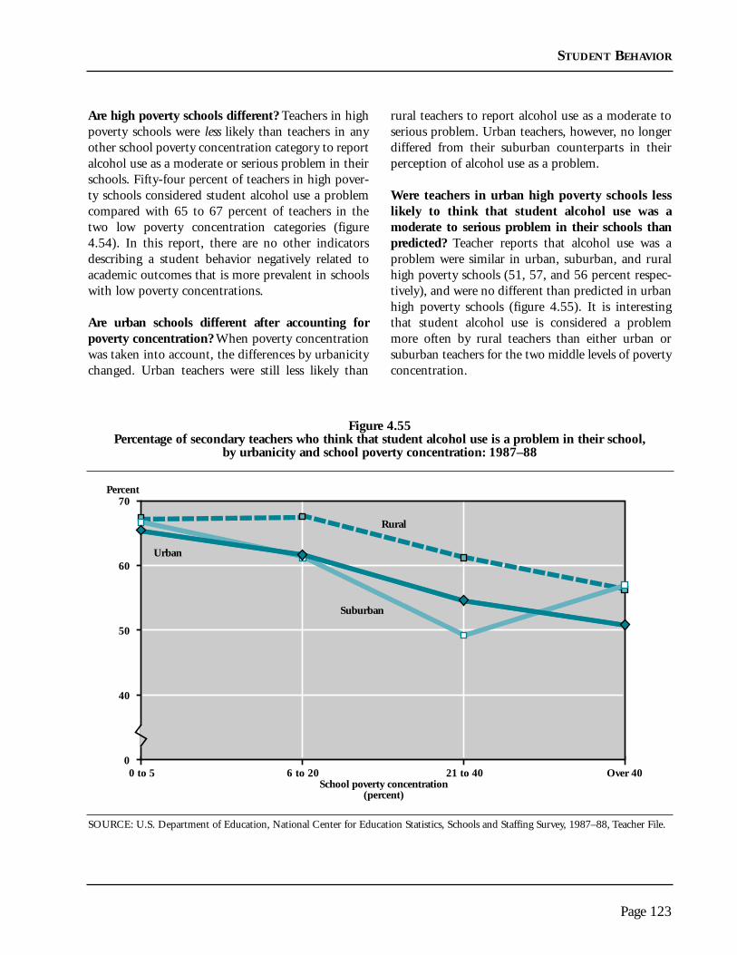
Are high poverty schools different? Teachers in highpoverty schools were less likely than teachers in anyother school poverty concentration category to reportalcohol use as a moderate or serious problem in theirschools. Fifty-four percent of teachers in high pover-ty schools considered student alcohol use a problemcompared with 65 to 67 percent of teachers in thetwo low poverty concentration categories (figure4.54). In this report, there are no other indicatorsdescribing a student behavior negatively related toacademic outcomes that is more prevalent in schoolswith low poverty concentrations.
Are urban schools different after accounting forpoverty concentration? When poverty concentrationwas taken into account, the differences by urbanicitychanged. Urban teachers were still less likely than
rural teachers to report alcohol use as a moderate toserious problem. Urban teachers, however, no longerdiffered from their suburban counterparts in theirperception of alcohol use as a problem.
Were teachers in urban high poverty schools lesslikely to think that student alcohol use was amoderate to serious problem in their schools thanpredicted? Teacher reports that alcohol use was aproblem were similar in urban, suburban, and ruralhigh poverty schools (51, 57, and 56 percent respec-tively), and were no different than predicted in urbanhigh poverty schools (figure 4.55). It is interestingthat student alcohol use is considered a problemmore often by rural teachers than either urban orsuburban teachers for the two middle levels of povertyconcentration.
Page 123
STUDENT BEHAVIOR
Figure 4.55Percentage of secondary teachers who think that student alcohol use is a problem in their school,
by urbanicity and school poverty concentration: 1987–88
Percent
0 to 5 6 to 20 21 to 40 Over 40
Suburban
Urban
Rural
0
40
50
60
70
School poverty concentration(percent)
SOURCE: U.S. Department of Education, National Center for Education Statistics, Schools and Staffing Survey, 1987–88, Teacher File.

Teenage pregnancy limits the educational opportunitiesof many female students, particularly those in poorurban settings. In addition, student pregnancy placessignificant demands on the social services of both theschool and the community (Males 1993; 1994; Caldas1994). This section examines how teachers perceive theproblem in their schools.
Are urban schools different? Nationally, 39 percent ofteachers in 1987-88 considered student pregnancy tobe a moderate or serious problem in their schools. Amuch larger percentage of urban teachers (48 percent)
considered this a problem when compared with subur-ban and rural teachers (30 percent and 38 percent,respectively) (figure 4.56).
Are high poverty schools different? Teachers’ percep-tions of the problem of pregnancy differed greatly byschool poverty concentration. Teachers in highpoverty schools were twice as likely to consider stu-dent pregnancy a moderate or serious problem thanteachers in low poverty schools (52 percent comparedwith 26 percent) (figure 4.57).
Page 124
STUDENT BEHAVIOR
Student Pregnancy
Percent
Total Urban Suburban Rural0
20
30
40
50
60
30.4
37.8
48.0
38.7
Percent
School poverty concentration(percent)
0 to 5 6 to 20 21 to 40 Over 400
20
30
40
50
60
Figure 4.56Percentage of secondary teachers who think thatstudent pregnancy is a problem in their school,
by urbanicity: 1987–88
Figure 4.57Percentage of secondary teachers who think thatstudent pregnancy is a problem in their school,
by school poverty concentration: 1987–88
SOURCE: U.S. Department of Education, National Center forEducation Statistics, Schools and Staffing Survey, 1987–88,Teacher File.
SOURCE: U.S. Department of Education, National Center forEducation Statistics, Schools and Staffing Survey, 1987–88,Teacher File.

Are urban schools different after accounting forpoverty concentration? After accounting for povertyconcentration, urban teachers were still more likely toconsider student pregnancy a problem than their coun-terparts in other locations. The higher concentration ofpoverty in urban schools is not the only explanation forthe greater prevalence of teacher concern about studentpregnancy in these schools.
Were teachers in urban high poverty schools morelikely to consider student pregnancy a moderate orserious problem in their schools than predicted?Teachers in urban high poverty schools were as likely
to consider student pregnancy a moderate or seriousproblem as predicted, given the poverty concentra-tion and location of their schools. Urban teachersreported this problem more frequently than theircounterparts at the middle two levels of school pover-ty concentration and more frequently than suburbanteachers in low poverty schools, but not more fre-quently than those in high poverty schools (figure4.58). There is no statistical difference between theproportion of teachers in urban high poverty schoolswho thought student pregnancy was a problem andthe proportion of teachers who thought so in otherhigh poverty schools.
Page 125
STUDENT BEHAVIOR
Figure 4.58Percentage of secondary teachers who think that student pregnancy is a problem in their school,
by urbanicity and school poverty concentration: 1987–88
Percent
0 to 5 6 to 20 21 to 40 Over 40
Suburban
Urban
Rural
0
20
30
40
50
60
School poverty concentration(percent)
SOURCE: U.S. Department of Education, National Center for Education Statistics, Schools and Staffing Survey, 1987–88, Teacher File.

Appendix A
Estimates and Standard Error Tables
Page A-1


Table 1.1—Data and standard errors for figures 1.1 and 1.2: Number and percentage distribution of studentsenrolled in public schools, by urbanicity: 1980 and 1990
School urbanicity Number Standard Percentage Standardand year (in millions) error distribution error
Total1980 40.4 0.1 100.0 —1990 37.7 0.1 100.0 —
Urban1980 10.6 0.2 26.3 0.41990 10.4 0.2 27.6 0.4
Suburban1980 16.5 0.2 40.8 0.31990 16.8 0.2 44.5 0.2
Rural1980 13.3 0.3 32.9 0.21990 10.5 0.3 27.9 0.2
— Not applicable.
SOURCE: U.S. Bureau of the Census, Current Population Survey, October 1980 and October 1990.
Page A-3

Table 1.2—Percentage of students in public and private schools, by urbanicity: 1987–88
StandardSchool urbanicity Percentage error
TotalPublic 88.4 0.2Private 11.6 0.2
Urban Public 83.4 0.6Private 16.6 0.6
SuburbanPublic 86.7 0.7Private 13.3 0.7
Rural Public 92.9 0.3Private 7.1 0.3
SOURCE: U.S. Department of Education, National Center for Education Statistics, Schools and Staffing Survey, 1987–88.
Page A-4

Table 1.3—Average school size, by urbanicity and level: 1987–88
School urbanicity Average Standardand level school size error
TotalElementary 424 3.5Middle/junior high 569 8.3Secondary 825 10.0
UrbanElementary 528 7.9Middle/junior high 735 17.0Secondary 1,313 31.0
SuburbanElementary 492 7.0Middle/junior high 662 21.0Secondary 1,197 30.0
RuralElementary 354 4.2Middle/junior high 463 11.0Secondary 577 11.0
SOURCE: U.S. Department of Education, National Center for Education Statistics, Schools and Staffing Survey, 1987–88.
Page A-5

Table 1.4—Data and standard errors for figures 1.3 and 1.8: Poverty rates for children under age 18, byurbanicity: 1980 and 1990, and percentage of students with difficulty speaking English, byurbanicity: 1979 and 1989
Rate or StandardUrbanicity and year Percentage error
TotalPoverty rate
1980 17.9 0.21990 19.9 0.4
Difficulty speaking English1979 2.7 0.11989 4.6 0.2
UrbanPoverty rate
1980 26.2 0.41990 30.0 0.9
Difficulty speaking English1979 6.2 0.31989 9.1 0.5
SuburbanPoverty rate
1980 11.2 0.21990 12.5 0.5
Difficulty speaking English 1979 1.9 0.21989 3.7 0.2
RuralPoverty rate
1980 19.4 0.31990 22.2 0.9
Difficulty speaking English1979 1.2 0.21989 1.9 0.3
SOURCE: U.S. Bureau of the Census, Current Population Reports, Series P–60, Nos. 181 and 133; and CurrentPopulation Survey, November 1979 and 1989.
Page A-6

Table 1.5—Data and standard errors for figure 1.4: Percentage of 8th graders whose family was in the lowestsocioeconomic quartile, by urbanicity and school poverty concentration: 1988
School urbanicity and Standardschool poverty concentration* Percentage error
Total 26.5 0.70 to 5% 13.0 1.36 to 20% 19.1 1.021 to 40% 26.8 1.1Over 40% 44.3 1.4
Urban—all 32.6 1.60 to 5% 17.8 5.96 to 20% 18.8 2.021 to 40% 26.0 3.2Over 40% 44.6 2.1
Suburban—all 19.1 1.00 to 5% 9.6 1.26 to 20% 14.8 1.121 to 40% 23.6 1.7Over 40% 44.4 3.4
Rural—all 31.9 1.10 to 5% 22.2 3.16 to 20% 27.3 1.921 to 40% 29.2 1.4Over 40% 44.0 2.3
*“School poverty concentration” refers to the percentage of students in the school receiving free and reduced price lunch.
NOTE: Totals may include a small proportion of students for whom school urbanicity and/or poverty concentration areunknown.
SOURCE: U.S. Department of Education, National Center for Education Statistics, National Education LongitudinalStudy of 1988, Base Year Survey.
Page A-7

Table 1.6—Data and standard errors for figure 1.5: Percentage of students in poverty-related programs, byurbanicity: 1987–88
Eligible for free or Receiving free or Receiving Chapter 1 reduced price lunch reduced price lunch services
School Per- Standard Per- Standard Per- Standardurbanicity centage error centage error centage error
Total 31.2 0.3 28.5 0.2 11.1 0.2
Urban 41.8 0.7 37.9 0.6 14.1 0.5
Suburban 17.9 0.4 16.2 0.4 6.8 0.5
Rural 30.6 0.3 28.3 0.3 11.2 0.2
SOURCE: U.S. Department of Education, National Center for Education Statistics, Schools and Staffing Survey, 1987–88.
Page A-8

Table 1.7—Data and standard errors for figure 1.6: Percentage distribution of students by school povertyconcentration within urbanicity categories: 1987–88
PercentageSchool urbanicity and distribution Standardschool poverty concentration* of students error
Total 100.0 —0 to 5% 17.2 0.46 to 20% 31.8 0.621 to 40% 25.0 0.5Over 40% 26.0 0.5
Urban—all 100.0 —0 to 5% 12.1 0.86 to 20% 25.8 1.221 to 40% 22.0 1.1Over 40% 40.1 1.1
Suburban—all 100.0 —0 to 5% 35.5 1.16 to 20% 38.7 1.121 to 40% 15.6 1.2Over 40% 10.2 0.8
Rural—all 100.0 —0 to 5% 11.7 0.56 to 20% 32.3 0.821 to 40% 31.5 0.7Over 40% 24.5 0.8
—Not applicable.*“School poverty concentration” refers to the percentage of students in the school receiving free and reduced price lunch.
SOURCE: U.S. Department of Education, National Center for Education Statistics, Schools and Staffing Survey, 1987–88.
Page A-9

Table 1.8—Data and standard errors for figure 1.7: Percentage distribution of students by school povertyconcentration deciles, by urbanicity: 1987–88
School urbanicity and Percentage distribution Standardschool poverty concentration* of students error
Urban—all 100.0 —0% 2.8 0.5 >0–10% 21.6 1.211–20% 13.7 0.821–30% 12.4 0.831–40% 9.4 0.641–50% 9.6 0.751–60% 6.3 0.461–70% 5.9 0.671–80% 5.9 0.681–90% 5.4 0.591–100% 7.0 0.6
Suburban—all 100.0 —0% 3.5 0.5>0–10% 50.0 1.311–20% 20.8 1.121–30% 9.4 0.931–40% 6.2 0.641–50% 3.3 0.551–60% 3.0 0.561–70% 1.7 0.471–80% 1.1 0.481–90% 0.6 0.291–100% 0.4 0.2
Rural—all 100.0 —0% 2.6 0.3>0–10% 21.9 0.611–20% 19.8 0.621–30% 18.2 0.631–40% 13.2 0.541–50% 9.1 0.651–60% 5.9 0.461–70% 3.7 0.371–80% 2.2 0.381–90% 2.0 0.391–100% 1.4 0.2
— Not applicable.*“School poverty concentration” refers to the percentage of students in the school receiving free and reduced price lunch.
SOURCE: U.S. Department of Education, National Center for Education Statistics, Schools and Staffing Survey,1987–88.
Page A-10

Table 1.9—Data and standard errors for figure 1.9: Trends in the racial-ethnic distribution of urbanstudents: 1980 and 1990
1980 1990Standard Standard
Race-ethnicity Percentage error Percentage error
White 48.5 0.3 42.7 0.4
Black 33.0 0.4 31.9 0.4
Hispanic 15.4 0.9 19.4 1.0
Other 3.1 1.4 6.0 1.3
NOTE: White refers to white, non-Hispanic students. Black refers to black, non-Hispanic students.
SOURCE: U.S. Bureau of the Census, Current Population Survey, October 1980 and October 1990.
Page A-11

Table 1.10—Data and standard errors for figures 1.10 and 1.11: Racial-ethnic distribution of students byurbanicity and school poverty concentration: 1987–88
School urbanicity White Black Hispanic Otherand school poverty Per- Standard Per- Standard Per- Standard Per- Standardconcentration1 centage error centage error centage error centage error
Total2
75.2 0.2 13.8 0.2 7.4 0.2 3.5 0.10 to 5% 87.7 0.7 5.4 0.5 3.3 0.3 3.5 0.26 to 20% 86.4 0.4 6.8 0.2 4.1 0.3 2.5 0.121 to 40% 81.6 0.5 9.8 0.4 5.7 0.3 2.6 0.2Over 40% 50.9 0.8 29.1 0.7 14.6 0.6 5.5 0.4
Urban—all 50.7 0.7 30.0 0.8 14.8 0.5 4.3 0.20 to 5% 73.8 2.3 14.4 2.0 6.8 1.0 4.6 0.76 to 20% 68.9 1.3 16.0 1.0 9.8 1.0 4.7 0.421 to 40% 60.3 1.3 22.9 1.3 11.3 0.9 4.3 0.4Over 40% 31.3 0.9 44.3 1.0 20.8 1.0 3.9 0.3
Suburban—all 79.4 0.6 10.3 0.4 6.2 0.4 3.8 0.20 to 5% 90.0 0.6 4.1 0.3 2.5 0.2 3.6 0.26 to 20% 84.5 0.7 7.2 0.5 4.6 0.4 3.4 0.221 to 40% 73.1 1.5 13.9 1.2 8.7 1.2 4.4 0.5Over 40% 42.9 2.6 32.9 2.6 18.4 2.3 5.1 1.4
Rural—all 83.5 0.4 8.4 0.2 4.9 0.2 3.1 0.20 to 5% 90.9 0.9 3.3 0.4 2.8 0.7 3.0 0.56 to 20% 92.6 0.4 3.8 0.3 2.2 0.2 1.4 0.121 to 40% 88.5 0.4 5.7 0.3 3.8 0.3 1.8 0.2Over 40% 64.6 1.0 18.8 0.7 10.0 0.8 6.5 0.6
1“School poverty concentration” refers to the percentage of students in the school receiving free and reduced price lunch.2Percentages may not add to 100 because of missing or miscoded data.
NOTE: White refers to white, non-Hispanic students. Black refers to black, non-Hispanic students.
SOURCE: U.S. Department of Education, National Center for Education Statistics, Schools and Staffing Survey, 1987–88.
Page A-12

Table 1.11—Percentage of students who belong to a racial-ethnic minority, by urbanicity and schoolpoverty concentration: 1987–88
School urbanicity and Standardschool poverty concentration* Percentage error
Total 24.7 0.20 to 5% 12.2 0.66 to 20% 13.4 0.421 to 40% 18.1 0.5Over 40% 49.2 0.8
Urban—all 49.0 0.60 to 5% 25.7 2.26 to 20% 30.5 1.321 to 40% 38.5 1.4Over 40% 69.0 0.9
Suburban—all 20.4 0.60 to 5% 10.1 0.66 to 20% 15.2 0.721 to 40% 27.0 1.6Over 40% 56.4 2.6
Rural—all 16.4 0.30 to 5% 9.1 0.96 to 20% 7.4 0.321 to 40% 11.3 0.4Over 40% 35.4 1.0
*“School poverty concentration” refers to the percentage of students in the school receiving free and reduced price lunch.
SOURCE: U.S. Department of Education, National Center for Education Statistics, Schools and Staffing Survey, 1987–88.
Page A-13

Table 1.12—Data and standard errors for figures 1.12–1.14: Selected measures of victimization and health,by urbanicity: 1988 and 1990
Rate or StandardUrbanicity percentage error
TotalVictimization rate, per 1,000 persons ages 12 and over
Crimes of violence, 1990 29.6 0.7Crimes of theft, 1990 63.8 1.0
Infant mortality rate, per 1000 live births, 1990 9.2 +/–0.1*Regular source of health care is a clinic, health center,or emergency room, ages 17 and under, 1988 15.5 0.4
Covered by health insurance/Medicaid, ages 17 andunder, 1988 83.1 0.4
UrbanVictimization rate, per 1,000 persons ages 12 and over
Crimes of violence 41.3 1.5Crimes of theft 81.5 2.1
Infant mortality rate, per 1000 live births, 1990 9.6 +/–0.1*Regular source of health care is a clinic, health center,or emergency room, ages 17 and under, 1988 23.3 0.9
Covered by health insurance/Medicaid, ages 17 andunder, 1988 81.5 0.8
SuburbanVictimization rate, per 1,000 persons ages 12 and over
Crimes of violence, 1990 25.2 1.0Crimes of theft, 1990 64.0 1.6
Infant mortality rate, per 1000 live births, 1990 7.8 +/–0.2*Regular source of health care is a clinic, health center,or emergency room, ages 17 and under, 1988 10.6 0.5
Covered by health insurance/Medicaid, ages 17 andunder, 1988 84.9 0.6
RuralVictimization rate, per 1,000 persons ages 12 and over
Crimes of violence, 1990 23.2 1.2Crimes of theft, 1990 43.4 1.7
Infant mortality rate, per 1000 live births, 1990 9.2 +/–0.2*Regular source of health care is a clinic, health center,or emergency room, ages 17 and under, 1988 15.5 0.9
Covered by health insurance/Medicaid, ages 17 andunder, 1988 81.7 0.9
*Random variation.
SOURCE: U.S. Department of Justice, Bureau of Justice Statistics, Criminal Victimization in the United States, 1990.National Center for Health Statistics, Vital Statistics of the United States, 1990, Vol. 2, Mortality, Public Health Service,Washington, D.C., Government Printing Office, 1993. U.S. Department of Health and Human Services, National Centerfor Health Statistics, Vital and Health Statistics, Advance Data, No. 188, Oct. 1, 1990.
Page A-14

Table 1.13—Percentage of girls scheduled to be in 12th grade1 who have or who are expecting a child, byurbanicity: 1992
School urbanicity and Standardschool poverty concentration2 Percentage error
Total 13.6 0.7
Urban 16.5 1.4
Suburban 10.3 1.2
Rural 14.2 1.0
1Includes girls who dropped out but would have been in 12th grade had they stayed in school and progressed normally.2“School poverty concentration” refers to the percentage of students in the school receiving free and reduced price lunch.
SOURCE: U.S. Department of Education, National Center for Education Statistics, National Education LongitudinalSurvey, Third Follow-up, 1992.
Page A-15

Table 2.1—Data and standard errors for figures 2.1–2.3: Average standardized test composite scores1 of8th-grade students, by urbanicity and school poverty concentration: 1988
School urbanicity and Composite Standardschool poverty concentration2 score error
Total 49.5 0.20 to 5% 52.7 0.46 to 20% 51.0 0.321 to 40% 49.3 0.3Over 40% 45.3 0.4
Urban—all 47.0 0.40 to 5% 50.8 1.46 to 20% 50.8 0.621 to 40% 47.6 0.6Over 40% 44.0 0.4
Suburban—all 50.8 0.30 to 5% 51.4 0.46 to 20% 51.1 0.421 to 40% 49.3 0.4Over 40% 45.6 0.6
Rural—all 49.4 0.30 to 5% 49.4 0.36 to 20% 50.9 0.521 to 40% 49.8 0.4Over 40% 46.5 0.7
1Standardized scores are transformations of the IRT-Estimated Number Correct scores, rescaled to a mean of 50 and stan-dard deviation of 10. The Standardized Test Composite is the equally weighted mean of the standardized reading and math-ematics scores, restandardized to a mean of 50 and standard deviation of 10. Because of missing data, the sample analyzedhere has a weighted mean of 49.5.2“School poverty concentration” refers to the percentage of students in the school receiving free and reduced price lunch.
NOTE: Totals may include a small proportion of students for whom school urbanicity is unknown.
SOURCE: U.S. Department of Education, National Center for Education Statistics, National Education LongitudinalStudy of 1988, Base Year Survey.
Page A-16

Table 2.2—Data and standard errors for figures 2.4–2.6: Average standardized test composite scores1 of10th-grade students, by urbanicity and school poverty concentration: 1990
School urbanicity and Composite Standardschool poverty concentration2 Score error
Total 50.0 0.20 to 5% 52.8 0.36 to 20% 50.6 0.321 to 40% 48.7 0.3Over 40% 45.1 0.3
Urban—all 48.8 0.40 to 5% 53.0 0.86 to 20% 50.3 0.821 to 40% 47.7 0.5Over 40% 44.7 0.6
Suburban—all 51.2 0.20 to 5% 53.0 0.36 to 20% 50.9 0.421 to 40% 47.4 0.9Over 40% 45.4 0.7
Rural—all 49.3 0.30 to 5% 50.9 1.16 to 20% 50.3 0.421 to 40% 49.6 0.5Over 40% 45.2 0.5
1Standardized scores are transformations of the IRT-Estimated Number Correct scores, rescaled to a mean of 50 and stan-dard deviation of 10. The Standardized Test Composite is the equally weighted mean of the standardized reading and math-ematics scores, restandardized to a mean of 50 and standard deviation of 10.2“School poverty concentration” refers to the percentage of students in the school receiving free and reduced price lunch.
NOTE: Totals may include a small proportion of students for whom school urbanicity and/or poverty concentration areunknown.
SOURCE: U.S. Department of Education, National Center for Education Statistics, National Education LongitudinalStudy of 1988, First Follow-up Survey, 1990.
Page A-17

Table 2.3—Data and standard errors for figure 2.7: Average number correct in mathematics for 10th-gradestudents, by urbanicity: 1980 and 1990, and 1980–1990 change
1980–19901980 1990 change
School Number Standard Number Standard Number Standardurbanicity correct error correct error correct error
Total 33.2 0.2 35.6 0.2 2.4 0.3
Urban 29.7 0.5 33.9 0.5 4.2 0.7
Suburban 33.7 0.3 37.2 0.3 3.5 0.4
Rural 31.7 0.3 34.9 0.3 3.2 0.4
NOTE: Totals may include a small proportion of students for whom school urbanicity is unknown.
SOURCE: U.S. Department of Education, National Center for Education Statistics, High School and Beyond, Base YearSurvey, 1980 and the National Education Longitudinal Study, First Follow-up Survey, 1990.
Page A-18

Table 2.4—Data and standard errors for figures 2.8–2.10: Percentage graduating on time among thesophomore class of 1980, by urbanicity and percent disadvantaged in school
School urbanicity and Standardpercent disadvantaged* Percentage error
Total 81.8 0.60 to 5% 85.5 0.96 to 20% 81.6 1.021 to 40% 79.7 1.7Over 40% 72.7 2.3
Urban—all 73.7 1.70 to 5% 80.3 3.36 to 20% 75.8 2.621 to 40% 71.6 3.7Over 40% 66.1 3.9
Suburban—all 84.3 0.90 to 5% 87.1 1.26 to 20% 82.6 1.421 to 40% 81.8 2.6Over 40% 74.0 4.1
Rural—all 83.3 0.90 to 5% 84.1 1.56 to 20% 83.4 1.521 to 40% 84.1 1.8Over 40% 80.1 2.8
*“Percent disadvantaged” refers to the percentage of students identified as disadvantaged by school administrators.
NOTE: Totals may include a small proportion of students for whom school urbanicity and/or percent disadvantaged areunknown.
SOURCE: U.S. Department of Education, National Center for Education Statistics, High School and Beyond Study, ThirdFollow-up, Spring 1986.
Page A-19

Table 2.5—Data and standard errors for figures 2.11–2.13: Percentage of young adults completing apostsecondary degree by 1990, by high school urbanicity and percent disadvantaged in highschool
School urbanicity and Standardpercent disadvantaged* Percentage error
Total 26.3 1.20 to 5% 36.2 2.16 to 20% 24.7 1.421 to 40% 19.5 2.0Over 40% 16.8 2.3
Urban—all 23.2 2.20 to 5% 26.6 6.76 to 20% 25.5 3.821 to 40% 23.3 4.3Over 40% 14.5 2.2
Suburban—all 30.2 1.80 to 5% 39.5 2.66 to 20% 24.9 2.121 to 40% 15.6 3.2Over 40% 17.1 4.1
Rural—all 21.7 1.70 to 5% 24.1 4.76 to 20% 24.0 2.221 to 40% 20.1 2.7Over 40% 17.7 3.7
*“Percent disadvantaged” refers to the percentage of students identified as disadvantaged by school administrators.
NOTE: Totals may include a small proportion of students for whom school urbanicity and/or percent disadvantaged areunknown.
SOURCE: U.S. Department of Labor, National Longitudinal Survey of Youth, 1990.
Page A-20

Table 2.6—Data and standard errors for figures 2.14–2.16: Percentage of young adults employed or attendingschool full time 4 years after high school, by high school urbanicity and percent disadvantaged inhigh school: 1986
School urbanicity and Standardpercent disadvantaged* Percentage error
Total 60.9 0.70 to5% 64.3 1.26 to 20% 62.1 1.121 to 40% 59.8 1.8Over 40% 47.6 2.5
Urban—all 56.6 1.50 to 5% 61.3 3.66 to 20% 60.6 2.821 to 40% 56.9 3.2Over 40% 46.9 3.2
Suburban—all 64.3 0.90 to 5% 66.6 1.46 to 20% 64.8 1.621 to 40% 57.1 3.9Over 40% 43.7 2.9
Rural—all 58.9 1.30 to 5% 60.5 2.56 to 20% 59.0 1.821 to 40% 63.2 2.6Over 40% 50.5 5.3
*“Percent disadvantaged” refers to the percentage of students identified as disadvantaged by school administrators.
NOTE: Totals may include a small proportion of students for whom school urbanicity and/or percent disadvantaged areunknown.
SOURCE: U.S. Department of Education, National Center for Education Statistics, High School and Beyond Study, ThirdFollow-up Survey, 1986.
Page A-21

Table 2.7—Data and standard errors for figures 2.17–2.19: Percentage of young adults employed or attendingschool full time, by high school urbanicity and percent disadvantaged in high school: 1990
School urbanicity and Standardpercent disadvantaged* Percentage error
Total 84.2 0.70 to 5% 87.5 1.16 to 20% 86.0 1.021 to 40% 80.9 1.6Over 40% 76.1 1.5
Urban—all 81.5 1.40 to 5% 87.1 3.06 to 20% 85.2 1.821 to 40% 79.0 3.0Over 40% 72.7 2.5
Suburban—all 86.4 0.70 to 5% 88.2 1.36 to 20% 86.0 1.321 to 40% 83.0 2.5Over 40% 80.8 4.4
Rural—all 82.3 1.30 to 5% 84.3 2.66 to 20% 86.3 2.221 to 40% 80.5 2.6Over 40% 76.0 1.5
*“Percent disadvantaged” refers to the percentage of students identified as disadvantaged by school administrators.
NOTE: Totals may include a small proportion of students for whom school urbanicity and/or percent disadvantaged areunknown.
SOURCE: U.S. Department of Labor, National Longitudinal Survey of Youth, 1990.
Page A-22

Table 2.8—Data and standard errors for figures 2.20–2.22: Percentage of young adults unemployed, byhigh school urbanicity and percent disadvantaged in high school: 1990
School urbanicity and Standardpercent disadvantaged* Percentage error
Total 3.6 0.30 to 5% 2.1 0.46 to 20% 3.4 0.521 to 40% 3.8 0.8Over 40% 7.6 1.2
Urban—all 5.8 0.80 to 5% 3.3 1.96 to 20% 4.5 1.121 to 40% 5.2 1.6Over 40% 10.8 1.7
Suburban—all 2.6 0.40 to 5% 1.9 0.56 to 20% 3.2 0.721 to 40% 2.2 1.0Over 40% 5.1 1.7
Rural—all 4.0 0.60 to 5% 2.3 1.06 to 20% 2.8 1.021 to 40% 4.1 1.2Over 40% 6.9 1.9
*“Percent disadvantaged” refers to the percentage of students identified as disadvantaged by school administrators.
NOTE: Totals may include a small proportion of students for whom school urbanicity and/or percent disadvantaged areunknown.
SOURCE: U.S. Department of Labor, National Longitudinal Survey of Youth, 1990.
Page A-23

Table 2.9—Data and standard errors for figures 2.23–2.25: Percentage of young adults living in poverty, byhigh school urbanicity and percent disadvantaged in high school: 1990
School urbanicity and Standardpercent disadvantaged* Percentage error
Total 8.3 0.50 to 5% 4.6 0.66 to 20% 8.0 0.721 to 40% 10.1 1.3Over 40% 14.7 2.1
Urban—all 14.5 1.40 to 5% 7.9 2.36 to 20% 11.3 1.821 to 40% 15.6 3.0Over 40% 25.5 3.0
Suburban—all 6.0 0.50 to 5% 3.7 0.86 to 20% 6.5 0.921 to 40% 9.3 2.4Over 40% 13.7 3.5
Rural—all 8.6 0.60 to 5% 7.6 2.16 to 20% 8.4 1.221 to 40% 8.2 1.5Over 40% 10.2 1.8
*“Percent disadvantaged” refers to the percentage of students identified as disadvantaged by school administrators.
NOTE: Totals may include a small proportion of students for whom school urbanicity and/or percent disadvantaged areunknown.
SOURCE: U.S. Department of Labor, National Longitudinal Survey of Youth, 1990.
Page A-24

Table 3.1—Data and standard errors for figures 3.1–3.3: Percentage of 8th-grade students living in atwo-parent family, by urbanicity and school poverty concentration: 1988
School urbanicity and Standardschool poverty concentration* Percentage error
Total 77.5 0.50 to 5% 85.0 0.86 to 20% 79.5 0.821 to 40% 76.6 0.9Over 40% 71.4 1.2
Urban—all 67.7 1.20 to 5% 80.7 3.26 to 20% 71.8 2.021 to 40% 68.2 2.9Over 40% 63.6 1.8
Suburban—all 80.7 0.60 to 5% 85.3 0.96 to 20% 81.2 1.021 to 40% 75.9 1.4Over 40% 77.4 1.7
Rural—all 79.6 0.70 to 5% 85.7 1.46 to 20% 80.9 1.321 to 40% 79.7 1.0Over 40% 75.8 1.8
*“School poverty concentration” refers to the percentage of students in the school receiving free and reduced price lunch.
NOTE: Totals may include a small proportion of students for whom school urbanicity and/or poverty concentration areunknown.
SOURCE: U.S. Department of Education, National Center for Education Statistics, National Education LongitudinalStudy of 1988, Base Year Survey.
Page A-25

Table 3.2—Data and standard errors for figures 3.4–3.6: Percentage of 8th-grade students living in a one-parent family with parent working full time, by urbanicity and school poverty concentration:1988
School urbanicity and Standardschool poverty concentration* Percentage error
Total 65.4 1.00 to 5% 74.4 2.66 to 20% 74.0 1.621 to 40% 65.2 1.9Over 40% 55.0 2.0
Urban—all 59.4 1.90 to 5% 60.6 8.56 to 20% 72.7 3.021 to 40% 64.4 4.3Over 40% 52.6 2.5
Suburban—all 71.3 1.60 to 5% 75.5 2.86 to 20% 78.1 2.321 to 40% 68.1 2.9Over 40% 51.7 4.6
Rural—all 64.6 1.90 to 5% 76.7 6.36 to 20% 67.6 3.321 to 40% 63.3 2.9Over 40% 61.3 4.2
*“School poverty concentration” refers to the percentage of students in the school receiving free and reduced price lunch.
NOTE: Totals may include a small proportion of students for whom school urbanicity and/or poverty concentration areunknown.
SOURCE: U.S. Department of Education, National Center for Education Statistics, National Education LongitudinalStudy of 1988, Base Year Survey.
Page A-26
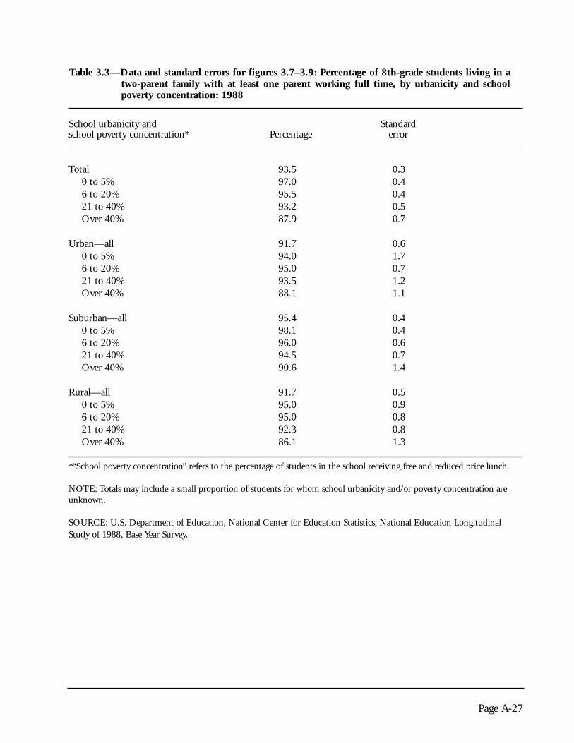
Table 3.3—Data and standard errors for figures 3.7–3.9: Percentage of 8th-grade students living in atwo-parent family with at least one parent working full time, by urbanicity and schoolpoverty concentration: 1988
School urbanicity and Standardschool poverty concentration* Percentage error
Total 93.5 0.30 to 5% 97.0 0.46 to 20% 95.5 0.421 to 40% 93.2 0.5Over 40% 87.9 0.7
Urban—all 91.7 0.60 to 5% 94.0 1.76 to 20% 95.0 0.721 to 40% 93.5 1.2Over 40% 88.1 1.1
Suburban—all 95.4 0.40 to 5% 98.1 0.46 to 20% 96.0 0.621 to 40% 94.5 0.7Over 40% 90.6 1.4
Rural—all 91.7 0.50 to 5% 95.0 0.96 to 20% 95.0 0.821 to 40% 92.3 0.8Over 40% 86.1 1.3
*“School poverty concentration” refers to the percentage of students in the school receiving free and reduced price lunch.
NOTE: Totals may include a small proportion of students for whom school urbanicity and/or poverty concentration areunknown.
SOURCE: U.S. Department of Education, National Center for Education Statistics, National Education LongitudinalStudy of 1988, Base Year Survey.
Page A-27

Table 3.4—Data and standard errors for figures 3.10–3.12: Percentage of 8th-grade students with aparent in the household who had completed 4 years of college, by urbanicity and schoolpoverty concentration: 1988
School urbanicity and Standardschool poverty concentration* Percentage error
Total 23.7 0.70 to 5% 41.5 2.26 to 20% 26.4 1.121 to 40% 20.1 0.9Over 40% 11.4 0.8
Urban—all 20.4 1.20 to 5% 32.5 6.46 to 20% 31.0 2.421 to 40% 23.1 2.4Over 40% 11.9 1.3
Suburban—all 29.5 1.20 to 5% 46.4 2.56 to 20% 28.5 1.621 to 40% 19.2 1.7Over 40% 10.4 1.4
Rural—all 18.6 0.90 to 5% 28.6 4.96 to 20% 19.8 1.521 to 40% 19.8 1.2Over 40% 11.6 1.2
*“School poverty concentration” refers to the percentage of students in the school receiving free and reduced price lunch.
NOTE: Totals may include a small proportion of students for whom school urbanicity and/or poverty concentration areunknown.
SOURCE: U.S. Department of Education, National Center for Education Statistics, National Education LongitudinalStudy of 1988, Base Year Survey.
Page A-28

Table 3.5—Data and standard errors for figures 3.13–3.15: Percentage of 8th-grade students who havechanged schools more than once since first grade, by urbanicity and school poverty concentra-tion: 1988
School urbanicity and Standardschool poverty concentration* Percentage error
Total 34.2 0.60 to 5% 30.5 1.36 to 20% 32.7 0.921 to 40% 34.6 1.2Over 40% 37.5 1.3
Urban—all 45.6 1.10 to 5% 38.8 2.96 to 20% 45.0 2.321 to 40% 47.2 2.3Over 40% 46.1 1.8
Suburban—all 33.6 0.80 to 5% 29.6 1.56 to 20% 32.2 1.221 to 40% 38.7 2.1Over 40% 37.3 2.5
Rural—all 28.0 0.90 to 5% 29.8 3.26 to 20% 26.2 1.621 to 40% 28.1 1.4Over 40% 28.9 1.8
*“School poverty concentration” refers to the percentage of students in the school receiving free and reduced price lunch.
NOTE: Totals may include a small proportion of students for whom school urbanicity and/or poverty concentration areunknown.
SOURCE: U.S. Department of Education, National Center for Education Statistics, National Education LongitudinalStudy of 1988, Base Year Survey.
Page A-29

Table 3.6—Data and standard errors for figures 3.16–3.18: Percentage of 8th-grade students whose parentsexpect them to complete 4 years of college, by urbanicity and school poverty concentration:1988
School urbanicity and Standardschool poverty concentration* Percentage error
Total 55.3 0.70 to 5% 66.2 1.96 to 20% 57.8 1.221 to 40% 51.3 1.0Over 40% 48.5 1.2
Urban—all 55.7 1.30 to 5% 61.0 7.86 to 20% 63.2 2.421 to 40% 55.2 1.8Over 40% 51.3 1.7
Suburban—all 60.2 1.10 to 5% 71.0 1.96 to 20% 60.6 1.721 to 40% 51.7 2.0Over 40% 47.4 2.3
Rural—all 49.0 1.00 to 5% 52.5 4.36 to 20% 49.0 1.721 to 40% 49.8 1.5Over 40% 46.2 2.1
*“School poverty concentration” refers to the percentage of students in the school receiving free and reduced price lunch.
NOTE: Totals may include a small proportion of students for whom school urbanicity and/or poverty concentration areunknown.
SOURCE: U.S. Department of Education, National Center for Education Statistics, National Education LongitudinalStudy of 1988, Base Year Survey.
Page A-30

Table 3.7—Data and standard errors for figures 3.19–3.21: Percentage of 8th-grade students whose parentsrarely talk to them about school, by urbanicity and school poverty concentration: 1988
School urbanicity and Standardschool poverty concentration* Percentage error
Total 21.7 0.40 to 5% 16.6 0.86 to 20% 20.0 0.621 to 40% 21.4 0.6Over 40% 27.6 0.9
Urban—all 24.9 0.90 to 5% 16.7 1.96 to 20% 21.3 1.621 to 40% 25.9 1.4Over 40% 27.6 1.5
Suburban—all 19.6 0.60 to 5% 16.0 0.96 to 20% 18.1 0.821 to 40% 21.1 1.1Over 40% 28.4 1.9
Rural—all 22.5 0.60 to 5% 18.6 1.76 to 20% 22.5 1.121 to 40% 20.2 0.9Over 40% 27.1 1.3
*“School poverty concentration” refers to the percentage of students in the school receiving free and reduced price lunch.
NOTE: Totals may include a small proportion of students for whom school urbanicity and/or poverty concentration areunknown.
SOURCE: U.S. Department of Education, National Center for Education Statistics, National Education LongitudinalStudy of 1988, Base Year Survey.
Page A-31

Table 3.8—Data and standard errors for figures 3.22–3.24: Average number of sports-related activities offeredby the schools attended by 10th-grade students, by urbanicity and school poverty concentration:1990
School urbanicity and Number of Standardschool poverty concentration* Activities error
Total 7.3 0.00 to 5% 7.8 0.16 to 20% 7.4 0.121 to 40% 6.9 0.1Over 40% 6.7 0.1
Urban—all 7.4 0.10 to 5% 7.3 0.46 to 20% 7.7 0.121 to 40% 7.4 0.1Over 40% 6.9 0.2
Suburban—all 7.7 0.10 to 5% 7.9 0.16 to 20% 7.7 0.121 to 40% 7.1 0.3Over 40% 7.1 0.2
Rural—all 6.7 0.10 to 5% 7.4 0.26 to 20% 7.0 0.221 to 40% 6.6 0.1Over 40% 6.2 0.2
*“School poverty concentration” refers to the percentage of students in the school receiving free and reduced price lunch.
NOTE: Totals may include a small proportion of students for whom school urbanicity and/or poverty concentration areunknown.
SOURCE: U.S. Department of Education, National Center for Education Statistics, National Education LongitudinalStudy of 1988, First Follow-up Survey.
Page A-32

Table 3.9—Data and standard errors for figures 3.25–3.27: Percentage of 10th-grade students who participatedin school sports-related activities, by urbanicity and school poverty concentration: 1990
School urbanicity and Standardschool poverty concentration* Percentage error
Total 51.6 0.70 to 5% 55.5 1.26 to 20% 52.1 1.121 to 40% 50.5 1.6Over 40% 43.5 1.8
Urban—all 45.0 1.40 to 5% 46.8 3.36 to 20% 45.2 2.521 to 40% 45.4 2.7Over 40% 40.1 3.3
Suburban—all 54.4 0.90 to 5% 57.1 1.46 to 20% 53.3 1.621 to 40% 45.1 2.9Over 40% 46.4 3.3
Rural—all 52.7 1.20 to 5% 54.0 3.56 to 20% 54.4 1.921 to 40% 55.1 2.4Over 40% 44.7 2.7
*“School poverty concentration” refers to the percentage of students in the school receiving free and reduced price lunch.
NOTE: Totals may include a small proportion of students for whom school urbanicity and/or poverty concentration areunknown.
SOURCE: U.S. Department of Education, National Center for Education Statistics, National Education LongitudinalStudy of 1988, First Follow-up Survey.
Page A-33

Table 3.10—Data and standard errors for figures 3.28–3.30: Percentage of 10th-grade students who worked11 or more hours per week, by urbanicity and school poverty concentration: 1990
School urbanicity and Standardschool poverty concentration* Percentage error
Total 18.4 0.50 to 5% 20.0 1.16 to 20% 20.1 0.921 to 40% 15.8 1.0Over 40% 14.4 1.3
Urban—all 18.3 1.10 to 5% 14.5 3.36 to 20% 21.7 2.221 to 40% 17.1 1.7Over 40% 17.8 2.4
Suburban—all 19.9 0.80 to 5% 20.4 1.26 to 20% 20.7 1.521 to 40% 18.8 2.6Over 40% 14.4 2.3
Rural—all 16.8 0.80 to 5% 22.2 3.16 to 20% 18.8 1.221 to 40% 14.3 1.3Over 40% 11.5 1.8
*“School poverty concentration” refers to the percentage of students in the school receiving free and reduced price lunch.
NOTE: Totals may include a small proportion of students for whom school urbanicity and/or poverty concentration areunknown.
SOURCE: U.S. Department of Education, National Center for Education Statistics, National Education LongitudinalStudy of 1988, First Follow-up Survey.
Page A-34

Table 4.1—Data and standard errors for figures 4.1–4.3: Percentage of teachers who agreed that necessarymaterials are available in their school, by urbanicity and school poverty concentration: 1987–88
School urbanicity and Standardschool poverty concentration* Percentage error
Total 76.3 0.30 to 5% 80.0 0.86 to 20% 77.7 0.621 to 40% 76.6 0.7Over 40% 71.5 0.6
Urban—all 70.1 0.70 to 5% 74.9 1.96 to 20% 72.7 1.421 to 40% 71.1 1.1Over 40% 66.9 0.8
Suburban—all 79.3 0.70 to 5% 82.9 1.06 to 20% 79.9 1.121 to 40% 73.8 1.9Over 40% 70.7 2.5
Rural—all 78.0 0.50 to 5% 78.5 1.46 to 20% 78.5 0.821 to 40% 79.1 0.9Over 40% 75.8 0.9
*“School poverty concentration” refers to the percentage of students in the school receiving free and reduced price lunch.
NOTE: Totals may include a small proportion of students for whom school urbanicity and/or poverty concentration areunknown.
SOURCE: U.S. Department of Education, National Center for Education Statistics, Schools and Staffing Survey, 1987–88,Teacher File.
Page A-35

Table 4.2—Data and standard errors for figures 4.4–4.6: Average years of teaching experience and averageacademic base year teacher salary, by urbanicity and school poverty concentration: 1987–88
Teacher experience Teacher salarySchool urbanicity and Average Standard Average Standardschool poverty concentration* years error dollars error
Total 14.6 0.0 $25,507 $ 72.40 to 5% 15.6 0.1 28,841 141.56 to 20% 14.7 0.1 25,896 147.721 to 40% 14.4 0.1 24,085 112.2Over 40% 13.8 0.1 24,179 131.2
Urban—all 15.0 0.1 27,372 150.80 to 5% 15.8 0.3 29,087 394.66 to 20% 15.0 0.2 27,565 304.621 to 40% 15.5 0.2 27,403 241.4Over 40% 14.5 0.2 26,772 253.4
Suburban—all 15.4 0.1 28,528 185.60 to 5% 16.3 0.2 30,470 256.96 to 20% 15.3 0.2 27,813 357.421 to 40% 14.6 0.3 26,759 379.4Over 40% 13.7 0.4 26,467 535.1
Rural—all 14.0 0.1 23,293 93.30 to 5% 14.6 0.2 26,530 284.96 to 20% 14.3 0.1 24,270 154.421 to 40% 13.9 0.1 22,426 122.3Over 40% 13.3 0.1 21,471 143.4
*“School poverty concentration” refers to the percentage of students in the school receiving free and reduced price lunch.
NOTE: Totals may include a small proportion of students for whom school urbanicity and/or poverty concentration areunknown.
SOURCE: U.S. Department of Education, National Center for Education Statistics, Schools and Staffing Survey, 1987–88,Teacher File.
Page A-36
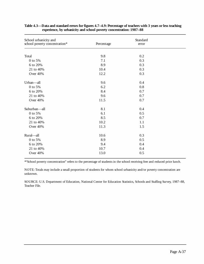
Table 4.3—Data and standard errors for figures 4.7–4.9: Percentage of teachers with 3 years or less teachingexperience, by urbanicity and school poverty concentration: 1987–88
School urbanicity and Standardschool poverty concentration* Percentage error
Total 9.8 0.20 to 5% 7.1 0.36 to 20% 8.9 0.321 to 40% 10.4 0.3Over 40% 12.2 0.3
Urban—all 9.6 0.40 to 5% 6.2 0.86 to 20% 8.4 0.721 to 40% 9.6 0.7Over 40% 11.5 0.7
Suburban—all 8.1 0.40 to 5% 6.1 0.56 to 20% 8.5 0.721 to 40% 10.2 1.1Over 40% 11.3 1.5
Rural—all 10.6 0.30 to 5% 8.9 0.56 to 20% 9.4 0.421 to 40% 10.7 0.4Over 40% 13.0 0.5
*“School poverty concentration” refers to the percentage of students in the school receiving free and reduced price lunch.
NOTE: Totals may include a small proportion of students for whom school urbanicity and/or poverty concentration areunknown.
SOURCE: U.S. Department of Education, National Center for Education Statistics, Schools and Staffing Survey, 1987–88,Teacher File.
Page A-37

Table 4.4—Data and standard errors for figures 4.10–4.12: Percentage of principals who report difficultyhiring teachers, by urbanicity and school poverty concentration: 1987–88
School urbanicity and Standardschool poverty concentration* Percentage error
Total 15.7 0.40 to 5% 11.4 1.26 to 20% 11.6 0.921 to 40% 13.1 0.8Over 40% 24.0 0.9
Urban—all 23.2 1.10 to 5% 11.2 2.56 to 20% 15.2 2.021 to 40% 19.2 2.1Over 40% 31.1 1.6
Suburban—all 13.2 0.90 to 5% 12.0 1.86 to 20% 10.9 1.321 to 40% 12.9 2.5Over 40% 25.7 4.0
Rural—all 13.4 0.70 to 5% 10.9 1.56 to 20% 10.8 1.121 to 40% 11.4 0.9Over 40% 19.1 1.5
*“School poverty concentration” refers to the percentage of students in the school receiving free and reduced price lunch.
NOTE: Totals may include a small proportion of students for whom school urbanicity and/or poverty concentration areunknown.
SOURCE: U.S. Department of Education, National Center for Education Statistics, Schools and Staffing Survey, 1987–88,Administrator File.
Page A-38

Table 4.5—Data and standard errors for figures 4.13–4.15: Percentage of teachers who are minority, byurbanicity and school poverty concentration: 1987–88
School urbanicity and Standardschool poverty concentration* Percentage error
Total 13.3 0.40 to 5% 5.9 0.66 to 20% 7.0 0.421 to 40% 9.2 0.6Over 40% 26.8 1.0
Urban—all 28.5 1.40 to 5% 16.8 2.86 to 20% 17.8 1.521 to 40% 23.4 2.7Over 40% 38.7 2.2
Suburban—all 10.1 0.70 to 5% 3.7 0.36 to 20% 6.7 0.621 to 40% 13.3 1.5Over 40% 28.5 2.5
Rural—all 8.1 0.30 to 5% 3.7 0.76 to 20% 3.7 0.421 to 40% 4.8 0.3Over 40% 18.7 0.7
*“School poverty concentration” refers to the percentage of students in the school receiving free and reduced price lunch.
NOTE: Totals may include a small proportion of students for whom school urbanicity and/or poverty concentration areunknown.
SOURCE: U.S. Department of Education, National Center for Education Statistics, Schools and Staffing Survey, 1987–88,Teacher File.
Page A-39

Table 4.6—Data and standard errors for figures 4.16–4.18: Percentage of secondary school teachers whoare male, by urbanicity and school poverty concentration: 1987–88
School urbanicity and Standardschool poverty concentration* Percentage error
Total 47.9 0.40 to 5% 50.7 0.96 to 20% 48.4 0.621 to 40% 45.7 0.8Over 40% 43.4 1.2
Urban—all 48.4 0.90 to 5% 54.0 2.46 to 20% 47.3 1.521 to 40% 46.0 1.8Over 40% 48.5 1.9
Suburban—all 48.8 0.90 to 5% 50.9 1.26 to 20% 47.2 1.421 to 40% 45.3 3.1Over 40% 41.5 4.7
Rural—all 47.1 0.70 to 5% 48.8 1.76 to 20% 49.2 0.921 to 40% 45.7 1.1Over 40% 39.3 1.8
*“School poverty concentration” refers to the percentage of students in the school receiving free and reduced price lunch.
NOTE: Totals may include a small proportion of students for whom school urbanicity and/or poverty concentration areunknown.
SOURCE: U.S. Department of Education, National Center for Education Statistics, Schools and Staffing Survey, 1987–88,Teacher File.
Page A-40

Table 4.7—Data and standard errors for figures 4.19–4.21: Percentage of teachers who think that teachershave a great deal of influence on establishing curriculum, by urbanicity and school poverty con-centration: 1987–88
School urbanicity and Standardschool poverty concentration* Percentage error
Total 34.9 0.40 to 5% 40.5 0.86 to 20% 37.5 0.621 to 40% 35.1 0.8Over 40% 27.6 0.6
Urban—all 26.0 0.70 to 5% 32.6 1.76 to 20% 30.1 1.421 to 40% 25.3 1.2Over 40% 21.9 1.0
Suburban—all 35.6 0.70 to 5% 41.0 1.26 to 20% 35.5 1.121 to 40% 28.4 2.4Over 40% 25.9 2.0
Rural—all 39.3 0.50 to 5% 43.7 1.46 to 20% 41.4 1.021 to 40% 39.7 0.9Over 40% 33.0 0.9
*“School poverty concentration” refers to the percentage of students in the school receiving free and reduced price lunch.
NOTE: Totals may include a small proportion of students for whom school urbanicity and/or poverty concentration areunknown.
SOURCE: U.S. Department of Education, National Center for Education Statistics, Schools and Staffing Survey, 1987–88,Teacher File.
Page A-41

Table 4.8—Data and standard errors for figures 4.22–4.24: Percentage of teachers who consider teacherabsenteeism a problem in their school, by urbanicity and school poverty concentration: 1987–88
School urbanicity and Standardschool poverty concentration* Percentage error
Total 23.4 0.40 to 5% 20.8 0.96 to 20% 22.0 0.721 to 40% 25.0 0.9Over 40% 31.1 1.4
Urban—all 30.6 0.70 to 5% 24.3 2.36 to 20% 29.5 2.021 to 40% 31.7 1.7Over 40% 37.0 2.4
Suburban—all 23.4 0.90 to 5% 20.7 1.16 to 20% 24.3 1.321 to 40% 30.8 3.5Over 40% 35.3 4.3
Rural—all 19.6 0.60 to 5% 19.1 1.56 to 20% 18.2 1.021 to 40% 20.4 1.0Over 40% 25.5 1.8
*“School poverty concentration” refers to the percentage of students in the school receiving free and reduced price lunch.
NOTE: Totals may include a small proportion of students for whom school urbanicity and/or poverty concentration areunknown.
SOURCE: U.S. Department of Education, National Center for Education Statistics, Schools and Staffing Survey, 1987–88,Teacher File.
Page A-42

Table 4.9—Data and standard errors for figures 4.25–4.27: Percentage of 8th-grade students who attendedpreschool, by urbanicity and school poverty concentration: 1988
School urbanicity and Standardschool poverty concentration* Percentage error
Total 51.1 0.80 to 5% 64.3 1.96 to 20% 53.9 1.321 to 40% 46.9 1.3Over 40% 39.8 1.5
Urban—all 52.7 1.40 to 5% 56.6 7.16 to 20% 59.4 2.121 to 40% 57.9 2.2Over 40% 44.9 2.2
Suburban—all 58.3 1.20 to 5% 69.6 1.96 to 20% 56.3 1.921 to 40% 53.5 2.1Over 40% 39.9 3.7
Rural—all 40.3 1.30 to 5% 48.1 4.66 to 20% 45.6 2.521 to 40% 38.1 1.9Over 40% 34.0 2.1
*“School poverty concentration” refers to the percentage of students in the school receiving free and reduced price lunch.
NOTE: Totals may include a small proportion of students for whom school urbanicity and/or poverty concentration areunknown.
SOURCE: U.S. Department of Education, National Center for Education Statistics, National Education LongitudinalStudy of 1988, Base Year Parent File.
Page A-43

Table 4.10—Data and standard errors for figures 4.28–4.30: Percentage of elementary schools that offergifted and talented programs, by urbanicity and school poverty concentration: 1987–88
School urbanicity and Standardschool poverty concentration* Percentage error
Total 76.7 0.70 to 5% 82.9 2.16 to 20% 81.1 1.221 to 40% 78.3 1.2Over 40% 69.5 1.1
Urban—all 73.2 1.20 to 5% 80.2 3.36 to 20% 82.3 2.621 to 40% 79.9 3.1Over 40% 66.1 1.3
Suburban—all 84.1 1.20 to 5% 93.5 2.26 to 20% 84.2 2.021 to 40% 81.0 2.3Over 40% 70.6 3.8
Rural—all 75.5 1.00 to 5% 73.6 4.16 to 20% 79.1 1.621 to 40% 77.4 1.5Over 40% 71.8 1.7
*“School poverty concentration” refers to the percentage of students in the school receiving free and reduced price lunch.
NOTE: Totals may include a small proportion of students for whom school urbanicity and/or poverty concentration areunknown.
SOURCE: U.S. Department of Education, National Center for Education Statistics, Schools and Staffing Survey, 1987–88,School File.
Page A-44

Table 4.11—Data and standard errors for figures 4.31–4.32: Percentage of graduating high school seniors whotook 6 or more credits in vocational education, by urbanicity and school poverty concentration:1990
School urbanicity and Standardschool poverty concentration* Percentage error
Total 18.6 1.3
UrbanicityUrban 19.9 3.4Suburban 13.6 2.0Rural 24.7 2.3
School poverty concentration0 to 5% 15.2 2.86 to 20% 18.0 2.321 to 40% 29.4 3.1Over 40% 24.8 10.6
*“School poverty concentration” refers to the percentage of students in the school receiving free and reduced price lunch.
NOTE: Totals may include a small proportion of students for whom school urbanicity and/or poverty concentration areunknown.
SOURCE: U.S. Department of Education, National Center for Education Statistics, National Assessment of EducationalProgress, 1990 High School Transcript Study.
Page A-45

Table 4.12—Data and standard errors for figures 4.33–4.34: Percentage of graduating high school seniorswho took geometry, by urbanicity and school poverty concentration: 1990
School urbanicity and Standardschool poverty concentration* Percentage error
Total 67.8 2.1
UrbanicityUrban 57.4 4.7Suburban 72.8 2.4Rural 66.2 4.5
School poverty concentration0 to 5% 74.4 3.26 to 20% 64.7 4.721 to 40% 57.4 8.2Over 40% 60.4 6.3
*“School poverty concentration” refers to the percentage of students in the school receiving free and reduced price lunch.
NOTE: Totals may include a small proportion of students for whom school urbanicity and/or poverty concentration areunknown.
SOURCE: U.S. Department of Education, National Center for Education Statistics, National Assessment of EducationalProgress, 1990 High School Transcript Study.
Page A-46

Table 4.13—Data and standard errors for figures 4.35–4.37: Percentage of 10th-grade students who watch3 or more hours of television on weekdays, by urbanicity and school poverty concentration:1990
School urbanicity and Standardschool poverty concentration* Percentage error
Total 33.2 0.60 to 5% 26.0 1.16 to 20% 33.2 1.121 to 40% 36.8 1.5Over 40% 43.2 1.9
Urban—all 36.7 1.60 to 5% 22.4 3.36 to 20% 35.8 2.621 to 40% 37.4 2.4Over 40% 48.5 3.4
Suburban—all 29.6 0.90 to 5% 26.0 1.26 to 20% 31.3 1.521 to 40% 37.1 3.8Over 40% 38.7 3.5
Rural—all 35.4 1.10 to 5% 30.1 3.16 to 20% 34.0 1.921 to 40% 36.4 2.2Over 40% 41.4 2.8
*“School poverty concentration” refers to the percentage of students in the school receiving free and reduced price lunch.
NOTE: Totals may include a small proportion of students for whom school urbanicity and/or poverty concentration areunknown.
SOURCE: U.S. Department of Education, National Center for Education Statistics, National Education LongitudinalStudy of 1988, First Follow-up Student File.
Page A-47

Table 4.14—Data and standard errors for figures 4.38–4.40: Average number of hours 10th-grade studentsspend on homework per week, by urbanicity and school poverty concentration: 1990
School urbanicity and Average number Standardschool poverty concentration* of hours error
Total 7.4 0.10 to 5% 7.8 0.26 to 20% 7.4 0.121 to 40% 7.0 0.2Over 40% 6.5 0.2
Urban—all 7.3 0.20 to 5% 8.7 0.66 to 20% 7.6 0.321 to 40% 6.6 0.3Over 40% 6.5 0.4
Suburban—all 7.4 0.10 to 5% 7.7 0.26 to 20% 7.4 0.221 to 40% 6.1 0.4Over 40% 6.5 0.3
Rural—all 7.4 0.10 to 5% 8.1 0.56 to 20% 7.4 0.221 to 40% 7.6 0.2Over 40% 6.5 0.3
*“School poverty concentration” refers to the percentage of students in the school receiving free and reduced price lunch.
NOTE: Totals may include a small proportion of students for whom school urbanicity and/or poverty concentration areunknown.
SOURCE: U.S. Department of Education, National Center for Education Statistics, National Education LongitudinalStudy of 1988, First Follow-up Student File.
Page A-48

Table 4.15—Data and standard errors for figures 4.41–4.43: Percentage of secondary teachers who believe thatstudent absenteeism is a problem in their school, by urbanicity and school poverty concentration:1987–88
School urbanicity and Standardschool poverty concentration* Percentage error
Total 68.1 0.40 to 5% 64.6 1.26 to 20% 67.5 1.021 to 40% 70.2 0.9Over 40% 74.2 1.0
Urban—all 78.2 0.80 to 5% 73.2 2.76 to 20% 78.6 1.521 to 40% 77.7 1.7Over 40% 83.7 1.6
Suburban—all 68.4 1.10 to 5% 64.8 1.56 to 20% 70.0 1.821 to 40% 80.5 3.0Over 40% 81.7 6.6
Rural—all 62.6 0.70 to 5% 60.0 2.06 to 20% 62.1 1.421 to 40% 64.4 1.4Over 40% 65.0 1.9
*“School poverty concentration” refers to the percentage of students in the school receiving free and reduced price lunch.
NOTE: Totals may include a small proportion of students for whom school urbanicity and/or poverty concentration areunknown.
SOURCE: U.S. Department of Education, National Center for Education Statistics, Schools and Staffing Survey, 1987–88,Teacher File.
Page A-49

Table 4.16—Data and standard errors for figures 4.44–4.46: Percentage of teachers of 8th-grade studentswho spend at least 1 hour per week maintaining classroom order and discipline, by urbanicityand school poverty concentration: 1988
School urbanicity and Standardschool poverty concentration* Percentage error
Total 16.7 0.70 to 5% 12.2 1.36 to 20% 16.7 1.221 to 40% 15.9 1.4Over 40% 21.1 1.7
Urban—all 24.6 1.50 to 5% 11.3 3.16 to 20% 20.5 2.521 to 40% 26.4 2.8Over 40% 28.2 2.4
Suburban—all 16.4 1.00 to 5% 13.6 1.76 to 20% 17.8 1.721 to 40% 17.6 2.5Over 40% 18.0 3.6
Rural—all 12.6 1.20 to 5% 8.0 2.06 to 20% 12.2 2.221 to 40% 11.6 1.9Over 40% 16.1 2.8
*“School poverty concentration” refers to the percentage of students in the school receiving free and reduced price lunch.
NOTE: Totals may include a small proportion of students for whom school urbanicity and/or poverty concentration areunknown.
SOURCE: U.S. Department of Education, National Center for Education Statistics, National Educational LongitudinalStudy of 1988, Teacher File.
Page A-50

Table 4.17—Data and standard errors for figures 4.47–4.49: Percentage of 10th-grade students who do notfeel safe at school, by urbanicity and school poverty concentration: 1990
School urbanicity and Standardschool poverty concentration* Percentage error
Total 8.8 0.40 to 5% 5.8 0.56 to 20% 8.1 0.521 to 40% 11.5 0.9Over 40% 11.6 1.0
Urban—all 12.6 1.00 to 5% 5.6 1.76 to 20% 11.2 1.521 to 40% 16.4 1.6Over 40% 11.6 1.8
Suburban—all 7.8 0.50 to 5% 6.1 0.66 to 20% 7.7 0.821 to 40% 15.7 3.4Over 40% 11.4 1.9
Rural—all 7.5 0.50 to 5% 4.7 1.36 to 20% 6.8 0.821 to 40% 7.4 0.9Over 40% 11.7 1.6
*“School poverty concentration” refers to the percentage of students in the school receiving free and reduced price lunch.
NOTE: Totals may include a small proportion of students for whom school urbanicity and/or poverty concentration areunknown.
SOURCE: U.S. Department of Education, National Center for Education Statistics, National Education LongitudinalStudy of 1988, First Follow-up Student File.
Page A-51
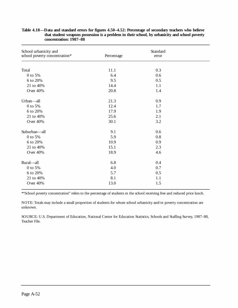
Table 4.18—Data and standard errors for figures 4.50–4.52: Percentage of secondary teachers who believethat student weapons possession is a problem in their school, by urbanicity and school povertyconcentration: 1987–88
School urbanicity and Standardschool poverty concentration* Percentage error
Total 11.1 0.30 to 5% 6.4 0.66 to 20% 9.5 0.521 to 40% 14.4 1.1Over 40% 20.8 1.4
Urban—all 21.3 0.90 to 5% 12.4 1.76 to 20% 17.9 1.921 to 40% 25.6 2.1Over 40% 30.1 3.2
Suburban—all 9.1 0.60 to 5% 5.9 0.86 to 20% 10.9 0.921 to 40% 15.1 2.3Over 40% 18.9 4.6
Rural—all 6.8 0.40 to 5% 4.0 0.76 to 20% 5.7 0.521 to 40% 8.1 1.1Over 40% 13.0 1.5
*“School poverty concentration” refers to the percentage of students in the school receiving free and reduced price lunch.
NOTE: Totals may include a small proportion of students for whom school urbanicity and/or poverty concentration areunknown.
SOURCE: U.S. Department of Education, National Center for Education Statistics, Schools and Staffing Survey, 1987–88,Teacher File.
Page A-52

Table 4.19—Data and standard errors for figures 4.53–4.55: Percentage of secondary teachers who think thatstudent alcohol use is a problem in their school, by urbanicity and school poverty concentration:1987–88
School urbanicity and Standardschool poverty concentration* Percentage error
Total 62.7 0.50 to 5% 66.6 0.96 to 20% 64.9 0.821 to 40% 58.3 1.1Over 40% 53.9 1.6
Urban—all 58.2 1.20 to 5% 65.7 2.16 to 20% 61.5 1.621 to 40% 54.7 2.2Over 40% 50.7 3.1
Suburban—all 62.7 1.20 to 5% 66.4 1.66 to 20% 61.3 1.721 to 40% 49.2 3.2Over 40% 57.1 5.6
Rural—all 64.6 0.50 to 5% 67.4 1.76 to 20% 67.6 1.021 to 40% 61.7 1.1Over 40% 56.1 2.4
*“School poverty concentration” refers to the percentage of students in the school receiving free and reduced price lunch.
NOTE: Totals may include a small proportion of students for whom school urbanicity and/or poverty concentration areunknown.
SOURCE: U.S. Department of Education, National Center for Education Statistics, Schools and Staffing Survey, 1987–88,Teacher File.
Page A-53

Table 4.20—Data and standard errors for figures 4.56–4.58: Percentage of secondary teachers who think thatstudent pregnancy is a problem in their school, by urbanicity and school poverty concentration:1987–88
School urbanicity and Standardschool poverty concentration* Percentage error
Total 38.7 0.60 to 5% 26.4 1.26 to 20% 39.0 1.021 to 40% 45.7 1.5Over 40% 52.2 1.8
Urban—all 48.0 1.30 to 5% 33.5 3.26 to 20% 45.0 2.321 to 40% 56.4 2.1Over 40% 55.8 3.0
Suburban—all 30.4 1.20 to 5% 22.2 1.46 to 20% 37.8 1.821 to 40% 40.9 5.0Over 40% 55.1 6.7
Rural—all 37.8 0.80 to 5% 29.0 1.76 to 20% 37.0 1.321 to 40% 40.4 1.6Over 40% 48.7 2.3
*“School poverty concentration” refers to the percentage of students in the school receiving free and reduced price lunch.
NOTE: Totals may include a small proportion of students for whom school urbanicity and/or poverty concentration areunknown.
SOURCE: U.S. Department of Education, National Center for Education Statistics, Schools and Staffing Survey, 1987–88,Teacher File.
Page A-54

There are four basic steps to the analysis for thisreport. Each answers a specific question:
1) Are urban schools different?
2) Are high poverty schools different?
3) Are urban schools different after taking intoaccount the poverty concentration of the school?
4) Are urban high poverty schools different thanpredicted? Is there something about theseschools that puts the students at particular riskfor poor educational outcomes and experiences?
Four models that correspond to these four questionscan be calculated. Each of the models uses the follow-ing notation:
Yi = the score on a particular outcome measurefor the ith student
X1i and X2i = a set of contrast-coded variables repre-senting the urbanicity of the ith student's schoolwhere:
X1i = 2 if suburban and -1 otherwise
X2i = 2 if rural and -1 otherwise
X3i, X4i, and X5i = a set of contrast-coded variablesrepresenting the poverty concentration of the ith stu-dent’s school where:
X3i = 3 if the school has 0 to 5 percent povertyconcentration and -1 otherwise
X4i = 3 if the school has 6 to 20 percent povertyconcentration and -1 otherwise
X5i = 3 if the school has 21 to 40 percent pover-ty concentration and -1 otherwise
X6i, X7i, X8i, X9i , X10i , and X11i = a set of variablesrepresenting various aspects of the interactionbetween urbanicity and poverty concentration where:
X6i = X1i * X3iX7i = X1i * X4iX8i = X1i * X5iX9i = X2i * X3iX10i = X2i * X4iX11i = X2i * X5i
Model 1 estimates:
Υi=β0+β1Χ1+β2Χ2
A joint test of β1+β2 tests the overall effect of urbanic-ity. If the overall test is significant, then a test thatβ1=0 tests the difference between students in rural andurban schools on Y, while the test that β2 = 0 tests thecontrast between students in suburban and urban schools.
Model 2 estimates:
Yi =β0+β3 Χ3+β4 Χ4+β5 Χ5
A joint test of β3+β4+β5 tests the overall effect ofpoverty concentration. If the overall test is significant,then a test that β3=0 tests the difference on Y betweenstudents in schools with 0 to 5 percent poverty con-centration and students in schools with over 40 per-cent poverty concentration; a test that β4=0 tests thedifference on Y between students in schools with 6 to20 percent poverty concentration and students inschools with over 40 percent poverty concentration;and a test that β5=0 tests the difference on Y betweenstudents in schools with 21 to 40 percent povertyconcentration and students in schools with over 40percent poverty concentration.
Model 3 estimates:
Yi =β0+β1 Χ1+β2 Χ2+β3 Χ3+β4 Χ4+β5 Χ5
Page B-1
Appendix B
Methodology of Analysis
^
^
^
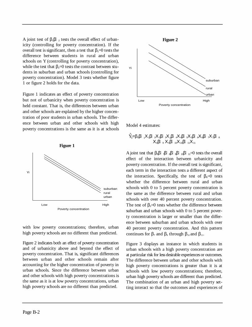
A joint test of β1+β2 tests the overall effect of urban-icity (controlling for poverty concentration). If theoverall test is significant, then a test that β1=0 tests thedifference between students in rural and urbanschools on Y (controlling for poverty concentration),while the test that β2=0 tests the contrast between stu-dents in suburban and urban schools (controlling forpoverty concentration). Model 3 tests whether figure1 or figure 2 holds for the data.
Figure 1 indicates an effect of poverty concentrationbut not of urbanicity when poverty concentration isheld constant. That is, the differences between urbanand other schools are explained by the higher concen-tration of poor students in urban schools. The differ-ence between urban and other schools with highpoverty concentrations is the same as it is at schools
with low poverty concentrations; therefore, urbanhigh poverty schools are no different than predicted.
Figure 2 indicates both an effect of poverty concentrationand of urbanicity above and beyond the effect ofpoverty concentration. That is, significant differencesbetween urban and other schools remain afteraccounting for the higher concentration of poverty inurban schools. Since the difference between urbanand other schools with high poverty concentrations isthe same as it is at low poverty concentrations, urbanhigh poverty schools are no different than predicted.
Model 4 estimates:
Yi=β0+β1Χ1+β2Χ2+β3Χ3+β4Χ4+β5Χ5+β6Χ6+β7Χ7+β8
Χ8+β9 Χ9+β10Χ10+β11Χ11
A joint test that β6+β7+β8+β9+β10+β11=0 tests the overalleffect of the interaction between urbanicity andpoverty concentration. If the overall test is significant,each term in the interaction tests a different aspect ofthe interaction. Specifically, the test of β6=0 testswhether the difference between rural and urbanschools with 0 to 5 percent poverty concentration isthe same as the difference between rural and urbanschools with over 40 percent poverty concentration.The test of β9=0 tests whether the difference betweensuburban and urban schools with 0 to 5 percent pover-ty concentration is larger or smaller than the differ-ence between suburban and urban schools with over40 percent poverty concentration. And this patterncontinues for β7 and β8 through β10 and β11.
Figure 3 displays an instance in which students inurban schools with a high poverty concentration are at particular risk for less desirable experiences or outcomes.The difference between urban and other schools withhigh poverty concentrations is greater than it is atschools with low poverty concentrations; therefore,urban high poverty schools are different than predicted.The combination of an urban and high poverty set-ting interact so that the outcomes and experiences of
Page B-2
Yi
Low High
suburban
rural
urban
Poverty concentrationPoverty concentration
suburbanruralurban
Low High
Yi
Yi
Low High
suburban
rural
urban
Poverty concentrationPoverty concentration
suburban
rural
urban
Low High
Yi
Figure 2
^
Figure 1

students in those settings are different than predicted.Also, students in urban high poverty schools are dif-ferent from students in other high poverty schools.
Of course, the actual data do not behave as simply asthe data in figures 1, 2, and 3, and the patterns can bequite complicated. In fact, sometimes the atypicalgroup is the advantaged urban students.
In addition, there is another simple pattern thatoccurs in the data—one that is not explicitly tested inmodels 1 through 4. This pattern is shown in figure 4.
In this case, there is an interaction between urbanici-ty and poverty concentration, but not the one explic-itly looked for in model 4. In fact, what is interestingis the lack of an overall effect of poverty concentrationon rural schools as compared with a quite markedeffect for urban and suburban schools. That is, whatis of interest here is the overall effect of poverty con-centration for rural schools, rather than the simplecontrast between high poverty concentration and lowpoverty concentration schools. One can hypothesize that the slopes of the lines defining the povertyconcentration are different for students in urban,suburban, and rural schools and that the slope for thestudents in rural schools is, in fact, not different fromzero. For example, assume we ran the following model:
Yi=β0+β1Χ1+β2Χ2+β3Χ3+β4Χ4+β5Χ5
where:
X1i and X2i = a set of contrast-coded variables repre-senting the urbanicity of the ith student’s school
where:
X1i=2 if suburban and -1 otherwiseX2i=2 if rural and -1 otherwiseX3i=poverty concentration expressed as a contin-uous variable (in most cases percent of free andreduced price lunch);
X4i and X5i = a set of variables representing the inter-action of urbanicity and poverty concentration with:
X4i = X1i * X3iX5i = X2i * X3i
A joint test of β4+β5 is now an overall test of the inter-action. Simple substitution of appropriate values forX1 through X5 results in the following simple regres-sion equations for students in urban, rural, and sub-urban schools:
Yurban=β0+β1(−1)+β2(−1)+β3(PCLNCH)+β4
(-1*PCLNCH)+β5(-1*PCLNCH)
Page B-3
Yi
Low High
suburban
rural
urban
Poverty concentrationPoverty concentration
suburban
rural
urban
Low High
Yi
urban
Yi
Lo Hi
suburban
rural
urban
Yi
Low gh
Poverty concentrationPoverty concentration
suburban
rural
urban
Low High
Yi
Figure 3 Figure 4
^
^

where:
(β3−β4−β5)*PCLNCH represents the poverty concen-tration slope for urban schools;
Yrural=β0+β1(2)+β2(-1)+β3(PCLNCH)+β4(2*PCLNCH)+β5(-1*PCLNCH)
where:
(β3+2β4−β5)*PCLNCH represents the poverty con-centration slope for rural schools; and
Ysuburban=β0+β1(−1)+β2(2)+β3(PCLNCH)+β4
(-1*PCLNCH)+β5(2*PCLNCH)where:
(β3−β4+2β5)*PCLNCH represents the poverty con-centration slope for suburban schools.
After calculating the appropriate standard errors(combining terms from the coefficients’ variance/covariance matrix), one can test whether the simpleslopes for urban, rural, and suburban schools differfrom one another, or whether they differ from zero.
Page B-4
^
^
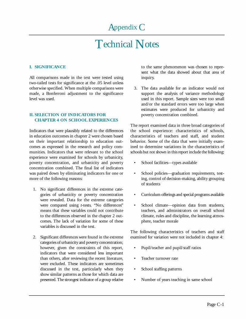
I. SIGNIFICANCE
All comparisons made in the text were tested usingtwo-tailed tests for significance at the .05 level unlessotherwise specified. When multiple comparisons weremade, a Bonferroni adjustment to the significancelevel was used.
II. SELECTION OF INDICATORS FOR CHAPTER 4 ON SCHOOL EXPERIENCES
Indicators that were plausibly related to the differencesin education outcomes in chapter 2 were chosen basedon their important relationship to education out-comes as expressed in the research and policy com-munities. Indicators that were relevant to the schoolexperience were examined for schools by urbanicity,poverty concentration, and urbanicity and povertyconcentration combined. The final list of indicatorswas paired down by eliminating indicators for one ormore of the following reasons:
1. No significant differences in the extreme cate-gories of urbanicity or poverty concentrationwere revealed. Data for the extreme categorieswere compared using t-tests. “No differences”means that these variables could not contributeto the differences observed in the chapter 2 out-comes. The lack of variation for some of thesevariables is discussed in the text.
2. Significant differences were found in the extremecategories of urbanicity and poverty concentration;however, given the constraints of this report,indicators that were considered less importantthan others, after reviewing the recent literature,were excluded. These indicators are sometimesdiscussed in the text, particularly when theyshow similar patterns as those for which data arepresented. The strongest indicator of a group relative
to the same phenomenon was chosen to repre-sent what the data showed about that area ofinquiry.
3. The data available for an indicator would notsupport the analysis of variance methodologyused in this report. Sample sizes were too smalland/or the standard errors were too large whenestimates were produced for urbanicity andpoverty concentration combined.
The report examined data in three broad categories ofthe school experience: characteristics of schools,characteristics of teachers and staff, and studentbehavior. Some of the data that were initially exam-ined to determine variations in the characteristics ofschools but not shown in this report include the following:
• School facilities—types available
• School policies—graduation requirements, test-ing, control of decision-making, ability groupingof students
• Curriculum offerings and special programs available
• School climate—opinion data from students,teachers, and administrators on overall schoolclimate, rules and discipline, the learning atmos-phere, teacher morale
The following characteristics of teachers and staffexamined for variation were not included in chapter 4:
• Pupil/teacher and pupil/staff ratios
• Teacher turnover rate
• School staffing patterns
• Number of years teaching in same school
Page C-1
Appendix C
Technical Notes

• Highest degree earned by teachers
• Number of courses taken by teachers in primaryand secondary field
• Certification in primary and secondary field
• Teacher benefits and pay incentives
• Professional development of teachers
• Instructional practices
• Teacher expectations for student achievement
• Ratings of teacher quality by students andadministrators
In the area of student behavior, the following issueswere analyzed in addition to those presented in theindicators section of this report:
• Average daily attendance/tardiness
• Student course selection
• Student effort on schoolwork and their ratingson difficulty of subject matter taught
• Outside reading
• Students’ perceived locus of control and self-concept indicators
• Students’ expectations for completing highschool and for attending college
• Delinquency
• Illegal substance abuse
• Physical conflicts/abuse of teachers
• Theft and robbery in school
Data for indicators that are not presented in the textcan be made available on request.
Page C-2

I. DATA SOURCES
National Education Longitudinal Study
The National Education Longitudinal Study of 1988(NELS:88) is a longitudinal survey that began in thespring of 1988 with a cohort of 24,599 8th graders. Atwo-stage stratified probability design was used toselect a nationally representative sample of schoolsand students. In the first stage, 1,734 schools wereselected, of which 1,052 (61 percent) participated—815 public and 237 private schools. From theseparticipating schools, 26,599 students (93 percent)participated in the survey. On average, each of theparticipating schools was represented by 23 students.The student, who filled out a background question-naire and completed an assessment test, is the basicunit of analysis in the NELS:88. All other componentsof the study—school, teacher, and parent questionnaires—are primarily intended to supplement the student dataset.
NCES has been conducting NELS follow-up surveysevery 2 years. This report uses data from the NELSBase Year Survey and the First Follow-up Survey,which was conducted in 1990 (when the studentswere generally in the 10th grade). For the FirstFollow-up Survey, several components were added,including a dropout study.
Schools and Staffing Survey
The Schools and Staffing Survey (SASS) is an integratedsurvey of schools, school districts, school administra-tors, and teachers designed to explore the major issuesconcerning the school work force and workplace. Asample of more than 9,300 public and 3,500 privateschools was drawn for the SASS that the NationalCenter for Education Statistics (NCES) conducted inthe 1987–88 school year. From these schools, a sampleof 56,000 public and 11,000 private school teachers
were selected. For this report, data from the 1987–88survey were used to construct several indicators. Inaddition to the 1987–88 survey, NCES also conductedthe SASS in the 1990–91 school year. Since SASSdoes not survey students, information on the studentsenrolled in a particular school is only availablethrough the items directed at the schools, schooladministrators, and teachers concerning the characteristicsof teachers and schools.
National Assessment of Educational Progress(NAEP) and NAEP High School Transcript Study
The National Assessment of Educational Progress(NAEP) is a federally funded periodic assessment ofthe educational achievement of students in varioussubject areas. The school and student samples for the1990 NAEP were selected using a complex multistagesampling design. The four stages included 1) selectionof geographically based Primary Sampling Units(PSUs); 2) selection of schools within sampling units;3) assignment of session types (these are based onassessment subjects) to schools; and 4) selection ofstudents for session types within schools. The result-ing samples were nationally representative of schoolsand students. The High School Transcript Study(HSTS), which was linked to the 1990 NAEP survey,included a representative sample of high schoolseniors who graduated in the 1990 calendar year. Thefile includes high school transcripts of approximately21,500 students from 330 schools; 16,456 of thesestudents were from public schools. To increase thereliability of estimates, private schools and publicschools with high enrollments of Hispanic or blackstudents were oversampled.
The schools included in the sample for the 1990HSTS included all schools with 12th grades that wereselected to participate in the 1990 NAEP assessmentwhether they participated or not. The students chosen,when possible, were the same students who partici-
Page D-1
Appendix D
Data Sources and Definitions

pated in the 1990 NAEP assessment. When this wasnot possible, such as cases where schools had notparticipated in the NAEP, a sample of students fromthose schools was drawn specifically for the HSTS.
High School and Beyond
High School and Beyond (HS&B) is a national longi-tudinal survey of high school sophomores and seniorsconducted by NCES. HS&B is a stratified nationalprobability sample of students. For the first stage ofthe HS&B, a sample of public and private highschools was selected. In the second stage, 36 seniorsand 36 sophomores were selected in each school. (Inschools with fewer than 36 students in either of thesegroups, all eligible students were included.) Certaintypes of schools were oversampled to make the studymore useful for policy analysis: public schools with ahigh percentage of Hispanic students, Catholicschools with a high percentage of minority students,alternative public schools, and private schools withhigh achieving students. In 1980, more than 30,000sophomores and 28,000 seniors enrolled in 1,015public and private high schools participated in theBase Year Survey. The survey instruments used in theBase Year Survey included a sophomore questionnaire,a senior questionnaire, a school questionnaire, ateacher comment checklist, and a parent questionnaire.HS&B participants have been followed through the1980s (1982, 1984, and 1986) and into the 1990s,with the Fourth Follow-up of the 1980 sophomorestaking place in 1992.
Technical Note
The weight (panelwt4) applied to the data reportedhere is the weight used for cases with data from all ofthe HS&B surveys: the Base Year, First Follow-up,Second Follow-up and Third Follow-up. This isnecessary because the samples drawn for the follow-up surveys were not the same as the original base yearsample. The base year sample included 28,000 sophomoresfrom 1,015 schools with a target number of 36 stu-dents from each school. For the First Follow-up,30,000 people who were 1980 sophomores wereselected. The Second and Third Follow-up sophomore
cohort samples were the same, totaling 15,000. Theresponse rate for the 1984 survey was 92 percent, andfor the 1986 survey, it was 91 percent.
National Longitudinal Survey of Youth
The National Longitudinal Survey of Youth (NLSY),conducted by the Bureau of Labor Statistics, is alongitudinal survey of a representative sample of thenoninstitutionalized civilian and military populationborn between the years of January 1, 1957, throughDecember 31, 1964. They have been interviewed onan annual basis since 1979, with the most recentinterview year being 1996. Two special subsamples ofthe survey are 1) a supplemental sample that overrepresentsthe civilian Hispanic, black, and economically disad-vantaged non-black/non-Hispanic youth living in theUnited States; and 2) a military sample representingthe youth population serving in the armed forces as ofSeptember 30, 1978, and born January 1, 1957,through December 31, 1961. Although a subsampleof the original military sample has been surveyed, themilitary sample was dropped in 1985 as a completesubsample.
In order to categorize respondents by the communitytype of the high school they attended, a separate filewas used that included an item for urbanicity derivedfrom the HS&B survey. This file contains data onlyfor respondents who attended public high schools.
II. DEFINITION OF URBANICITY ANDPOVERTY CONCENTRATION IN SURVEYS
Although every effort was made to categorize schoolsby the same criteria for location and poverty concen-tration across all of the surveys used in this report, theway in which these two variables were defined in eachof the data sources does vary. Below is a brief descriptionof the definition of these two variables for each datasource analyzed.
National Education Longitudinal Study
School urbanicity, either urban, suburban, or rural,for the Base Year Survey of NELS was based on urban-
Page D-2

icity assigned to schools in the frame used to createthe NELS sample, and corresponds to U.S. Bureau ofthe Census classifications. For this survey, the QualityEducation Data (QED), a universe database of publicand private parochial and nonparochial schools in theUnited States, was used. When urbanicity data wereunavailable from the QED, Bureau of the Census datawere used. For the NELS 10th-grade Follow-upSurvey, the same source for school location data wasused to ensure comparability with the 1988 survey.Schools classified as urban are located in central citiesof Metropolitan Statistical Areas (MSAs); schools clas-sified as suburban are located within the area sur-rounding a central city within a county constitutingthe MSA; and schools classified as rural are outside of anMSA.
For poverty concentration, the 1988 base year schooladministrators were asked to report the number of stu-dents receiving free or reduced price lunches. For theanalysis in this report, the number reported wasdivided by the total school enrollment to get the per-centage of students receiving free or reduced pricelunch. This resulted in school poverty concentrationsthat were similar in distribution to those produced bythe SASS. However, for the 10th-grade follow-up,school administrators were asked to list the percentageof students receiving free or reduced price lunch. Theresulting distribution of schools matches more closelythe data on the percentage of disadvantaged studentsreported for the HS&B and the NLSY databases.
Schools and Staffing Survey
Respondents reported on the urbanicity of schools inthe school questionnaire administered as part of the1987–88 SASS, while in the other surveys (NELS,NAEP, HS&B, and NLSY) school urbanicity wasassigned to the school based upon the address. Allsubsequent administrations of the SASS survey haveused a locale code assigned to the school based uponits address. As of the publication of this report, thesecodes have been added to the 1987–88 data to enablecomparisons between the different administrations ofSASS. In 1987–88, the SASS respondents chose from10 residence categories, ranging in size from a rural orfarming community to a very large city of more than
500,000 people. For this report, the 10 categorieshave been collapsed into the same three urbanicitycategories (urban, suburban, and rural) as were usedin the other data sets. Three city sizes in SASS—rangingfrom a medium-sized city of 50,000 to 100,000 people,a large city of 100,000 to 500,000 people, or a verylarge city of more than 500,000 people—have beencollapsed into one urban group comprised of cities of50,000 people or more. The suburbs of each of thesecities have been collapsed into one suburban category,with military bases or stations added to this group.One rural category has been created from the followingthree groups: a rural or farming community, a smallcity or town of fewer than 50,000 people that is not asuburb of a larger city, or an Indian reservation.
The self-reported urbanicity in the 1987–88 SASSresults in noticeable differences in how schools arecategorized when compared with data on school locationfrom other sources. Although the number of urbanschools appears to be roughly comparable between the1987–88 SASS and other data sources, the number ofschools classified as rural is higher, and consequently,the number of suburban schools is lower, when com-pared with Bureau of the Census location data. Forexample, according to 1990 Bureau of the Censusdata presented in appendix table 1.1, 28 percent of pub-lic school students attended urban schools, 45 percentattended suburban, and 28 percent attended ruralschools. However, according to the comparable SASSenrollment data for 1987–88 using the school-reportedlocation, 30 percent of public school enrollment is inurban schools, 23 percent in suburban, and 47percent in rural.
Poverty concentration for the SASS survey wasdefined as “the percentage of students in the schoolreceiving free or reduced price lunch.” This figure wascalculated by using the number of students receivinglunches divided by the total enrollment.
National Assessment of Educational Progress(NAEP) and NAEP High School Transcript Study
The urbanicity of schools in the National Assessmentof Educational Progress (NAEP) High SchoolTranscript Study (HSTS) survey was assigned to
Page D-3

schools based on school address using 1980 Bureau ofCensus data and definitions of urban, suburban, andrural areas. Schools classified as urban are located incentral cities of Metropolitan Statistical Areas(MSAs); schools classified as suburban are locatedwithin the area surrounding a central city within acounty constituting the MSA; and schools classified asrural are outside of an MSA.
The definition of poverty concentration used for theNAEP survey, which was linked to the HSTS, was thepercentage of students in a school receiving free orreduced price lunch which was derived from estimatesby the school administrator who filled out thequestionnaire.
High School and Beyond
School urbanicity was assigned to schools in the HighSchool and Beyond (HS&B) survey based on 1980Bureau of the Census data and definitions for urban,suburban, and rural areas. Schools classified as urbanare located in central cities of Metropolitan StatisticalAreas (MSAs); schools classified as suburban are locat-ed within the area surrounding a central city within acounty constituting the MSA; and schools classified asrural are outside of an MSA.
School poverty concentration was derived fromschool administrator responses to a school question-naire item asking first what criteria, whether federal,state, or other guidelines, were used to classify studentsas disadvantaged. Then the responding school officialwas asked to estimate the percentage of “disadvantaged”
students in the school, according to the guidelines ofChapter 1 of the Elementary and SecondaryEducation Act. This figure was used to classify schoolsinto the poverty concentration categories used in thisreport.
National Longitudinal Survey of Youth
School urbanicity was not a variable on the publicrelease file of the National Longitudinal Survey ofYouth (NLSY) survey. However, urbanicity codeswere matched to the respondent’s high school by theCenter for Human Resource Research at Ohio StateUniversity using the original HS&B sampling frame.School urbanicity was assigned to schools in theHS&B survey based on 1980 Bureau of the Censusdata and definitions for urban, suburban, and ruralareas. Schools classified as urban are located in centralcities of Metropolitan Statistical Areas (MSAs);schools classified as suburban are located within thearea surrounding a central city within a county con-stituting the MSA; and schools classified as rural areoutside of an MSA. For the purpose of this report,urbanicity codes for respondents in the nonmilitarysample who attended public high schools were madeavailable.
Poverty concentration was defined in the same manneras it was for the HS&B survey, as discussed above.School administrators were asked what percentage ofthe students in their school were classified as“disadvantaged” according to the guidelines ofChapter 1 of the Elementary and SecondaryEducation Act.
Page D-4

Abt Associates. 1993. Prospects: The Congressionally Mandated Study of Educational Growth and Opportunity.Washington, D.C.: U.S. Department of Education.
Anderson, J.; Hollinger, D.; and Conaty, J. 1992. “Poverty and Achievement: Re-examining the RelationshipBetween School Poverty and Student Achievement.” Paper presented at the Annual Meeting of the AmericanEducational Research Association.
Armor, D. J. 1972. “School and Family Effects on Black and White Achievement: A Re-examination of theUSOE Data.” In On Equality of Educational Opportunity. Frederick Mosteller and Daniel P. Moynihan, eds.New York: Vintage Books.
Ascher, C.; Burnett, G. 1993. Current Trends and Issues in Urban Education, 1993. Trends and Issues No. 19.New York: ERIC Clearinghouse on Urban Education.
Barro, S.; Kolstad, A. 1987. Who Drops Out of High School? Findings from High School and Beyond. Washington,D.C.: National Center for Education Statistics (CS 87-397c).
Bastian, L. D.; Taylor, B.M. 1991. School Crime: A National Crime Victimization Survey Report. Washington,D.C.: Bureau of Justice Statistics (NCJ-131645).
Berliner, D. 1993. “Mythology and the American System of Education,” Phi Delta Kappan, 74,(8), 632,634–40.
Bianchi, S. 1993. “Change in the Educational Performance of U.S. Children in the 1980s.” Working Papers fromthe Education Analysis Staff. Paper No. 93–2. Washington, D.C.: Bureau of the Census and National Center forEducation Statistics.
Bianchi, S.; McArthur, E. 1991. “Family Disruption and Economic Hardship: the Short-Run Picture forChildren.” Current Population Reports, Series P-70, Report No. 23.
Bobbitt, S. A.; Faupel, E.; and Burns, S. 1991. Stayers, Movers, and Leavers: Results of the 1988–89 TeacherFollowup Survey, 1991. Washington, D.C.: National Center for Education Statistics (NCES 91–128).
Bobbitt, S. A.; Quinn, P.; and Dabbs, P. 1992. Filling the Gaps: An Overview of Data on Education in Grades KThrough 12. Washington, D.C.: National Center for Education Statistics (NCES 92–132).
Braddock, J. H., II; et al. 1991. “Bouncing Back: Sports and Academic Resilience Among African-AmericanMales.” Education and Urban Society, 24 (1), 113–131.
Brooks-Gunn, J.; Duncan, G.; Klebanov, P.; and Sealand, N. 1993. “Do Neighborhoods Influence Child andAdolescent Development?” American Journal of Sociology, 99 (2), 353–395.
Page E-1
Appendix E
Bibliography

Caldas, S. J. 1994. “Teen Pregnancy: Why It Remains a Serious Social, Economic and Educational Problem inthe U.S.” Phi Delta Kappan, 75 (5), 402–406.
Carnegie Foundation for the Advancement of Teaching. 1988. An Imperiled Generation: Saving Urban Schools.Princeton, NJ: The Carnegie Foundation.
Choy, S. P.; Bobbitt, S. A.; Henke, R. R.; Medrich, E. A.; Horn, L. J.; and Lieberman, J. 1993a. America’sTeachers: Profile of a Profession. Washington, D.C.: National Center for Education Statistics (NCES 93-025).
Choy, S. P.; Henke, R. R.; Alt, M. N.; Medrich, E. A.; and Bobbitt, S. A. 1993b. Schools and Staffing in theUnited States: A Statistical Profile, 1990–91. Washington, D.C.: National Center for Education Statistics (NCES93-146).
Choy, S. P.; Medrich, E. A.; Henke, R. R.; and Bobbitt, S. A. 1992. Schools and Staffing in the United States: AStatistical Profile, 1987–88. Washington, D.C.: National Center for Education Statistics (NCES 92-120).
Clarke, R. L. 1992. “The Neighborhood Effects of Dropping Out of School among Teenage Boys.” Washington,D.C.: The Urban Institute.
Coleman, J. S.; Cambell, E. Q.; Hobson, C. S.; McPartland, J.; Mood, A. M.; Weinfeld, F. D.; York, R. L.;1966. Equality of Educational Opportunity. Washington, D.C.: U.S. Department of Health, Education andWelfare.
Coulton, C. J.; and Pandey, S. 1992. “Geographic Concentration of Poverty and Risk for Children in UrbanNeighborhoods.” American Behavioral Scientist, 25 (3), 238–257.
Council of the Great City Schools. 1994. National Urban Education Goals: 1992–93 Indicators Report.Washington, D.C.
Council of the Great City Schools. 1992. National Urban Education Goals: 1990–91 Indicators Report.Washington, D.C.
Crane, J. 1991. “The Epidemic Theory of Ghettos and Neighborhood Effects on Dropping Out and TeenageChildbearing.” American Journal of Sociology, 96 (5), 1226–1259.
Duncan, G. J.; Brooks-Gunn, J.; Klebanov, P. K. 1993. “Economic Deprivation and Early-ChildhoodDevelopment.” Child Development, 65 (2), 296–318.
Ellwood, D. 1988. Poor Support: Poverty in the American Family. New York: Basic Books.
Entwistle, D. Unpublished paper. 1990. “Recommendations for the NCES Longitudinal Study of EarlyChildhood Education.” Baltimore: The Johns Hopkins University.
Finn, J. D. 1993. School Engagement and Students at Risk. Washington, D.C.: National Center for EducationStatistics (NCES 93-470).
Page E-2

Fordham, S.; Ogbu, J. 1986. “Black Students’ School Success: Coping with the Burden of Acting White.” UrbanReview, 18 (3), 176–206.
Freeman, R. 1991. “Employment and Earnings of Disadvantaged Youth in a Labor Shortage Economy.” In C.Jencks and P. Peterson, eds., The Urban Underclass. Washington, D.C.: Brookings Institution.
Gamoran, A. 1987. “The Stratification of High School Learning Opportunities.” Sociology of Education, 60 (3),135–155.
Glazer, N. 1992. “The Real World of Urban Education.” Public Interest, 106, 57–75.
Greenberger, E.; Steinberg, L. 1986. When Teenagers Work: The Psychological and Social Costs of AdolescentEmployment. New York, NY: Basic Books, Inc.
Hanushek, E. A. 1994. “Money Might Matter Somewhere: A Response to Hedges, Laine and Greenwald.”Educational Researcher, 23 (4), 5–8.
Hanushek, E. A. 1989. “The Impact of Differential Expenditures on School Performance.” EducationalResearcher, 18 (4), 45–52.
Hartman, W. T. 1988. “District Spending Disparities: What Do the Dollars Buy?” Journal of Education Finance,13 (4), 436–458.
Haveman, R.; Wolfe, B. L.; Spaulding, J. 1991. “Childhood Events and Circumstances Influencing High SchoolCompletion.” Demography, 28 (2), 133–157.
Hedges, L. V.; Laine, R. D.; Greenwald, R. 1994. “Does Money Matter? A Meta Analysis of Studies of theEffects of Differential School Inputs on Student Outcomes.” Educational Researcher, 23 (3), 5–14.
Hedges, L. V.; Laine, R. D.; Greenwald, R. 1994. “Money Does Matter Somewhere: A Reply to Hanushek.”Educational Researcher, 23 (4), 9–10.
Hodgkinson, H. 1989. The Same Client: The Demographics of Education and Service Delivery Systems.Washington, D.C.: Institute for Educational Leadership and Center for Demographic Policy.
Hofferth, S. L.; West, J.; Henke, R.; and Kaufman, P. 1994. Access to Early Childhood Programs for Children atRisk. Washington, D.C.: National Center For Education Statistics (NCES 93-372).
Horn, L.; West, J. 1992. A Profile of Parents of Eighth Graders. Washington, D.C.: National Center for EducationStatistics (NCES 92-488).
Jencks, C.; Mayer, S. E. 1990. “Social Consequences of Growing Up in a Poor Neighborhood.” In Inner CityPoverty in the U.S. L. E. Lynn, Jr. and M. G. H. McGeary, eds. Washington, D.C.: National Academy Press.
Jones, L. K. 1992. The Encyclopedia of Career Change and Work Issues. Phoenix: Oryx Press.
Page E-3

Jordan, M. July 7, 1992. “Shortage of Minority Male Teachers Reported.” The Washington Post, A4.
Karweit, N. Unpublished paper. 1992. “Improving the Capacity of the National Education Statistical Databaseto Address Equity Issues.” Baltimore: Center for the Organization of Schools. The Johns Hopkins University.
Kaufman, P.; Bradby, D. 1992. Characteristics of At-Risk Students in NELS:88. Washington, D.C.: NationalCenter for Education Statistics (NCES 92-042).
Kennedy, M. M.; Jung, R. K.; and Orland, M.E. 1986. Poverty, Achievement and the Distribution ofCompensatory Education Services. Washington, D.C.: U.S. Department of Education.
King, S. H. 1993. “The Limited Presence of African-American Teachers.” Review of Educational Research, 63 (2),115–149.
Kirsch, I. S.; Jungeblut, A. 1986. Literacy: Profiles of America’s Young Adults. Princeton: National Assessment ofEducational Progress. Educational Testing Service. Report No. 16-PL-02.
Knepper, P. 1990. Trends in Postsecondary Credit Production, 1972 and 1980 High School Graduates. Washington,D.C.: National Center for Education Statistics (NCES 90-351).
Kozol, J. 1991. Savage Inequalities: Children in America’s Schools. New York: Crown Publishers.
Lewin-Epstein, N. 1981. Youth Employment During High School: An Analysis of High School and Beyond, aNational Longitudinal Study for the 1980s. Washington, D.C.: National Center for Education Statistics (NCES81-249).
Long, L. H. 1975. “Does Migration Interfere with Children’s Progress in School?” Sociology of Education, 48 (3), 369–381.
Louis, K. S.; Miles, M. B. 1990. Improving the Urban High School: What Works and Why. New York, NY:Teachers College Press.
Males, M. 1994. “Poverty, Rape, Adult/Teen Sex.” Phi Delta Kappan, 75 (5), 407–410.
Males, M. 1993. “Schools, Society and ‘Teen’ Pregnancy.” Phi Delta Kappan, 74 (7), 566–68.
Mangum, G. L. 1988. “Youth Transition from Adolescence to the World of Work.” prepared for Youth andAmerica’s Future: The William T. Grant Foundation Commission on Work, Family and Citizenship, 1988.
Massey, D.; Gross, A. B.; and Shibuya, K. 1994. “Migration, Segregation, and the Concentration of Poverty.”American Sociological Review, 59 (3), 425–445.
Mayer, S.E.; Jencks, C. 1989. “Growing Up in Poor Neighborhoods: How Much Does it Matter?” Science, 243(4897), 1441–1445.
McArthur, E. 1993. Language Characteristics and Schooling in the United States: A Changing Picture: 1979 and1989. Washington D.C.: National Center for Education Statistics (NCES 93-699).
Page E-4
McFadden, R. D. October 15, 1993. “Twenty Percent of New York City Public-School Students CarryWeapons, Study Finds.” The New York Times, B3.
Mulkey, L. M.; Crain, R. L.; Harrington, A. J. C. 1992. “One-Parent Households and Achievement: Economicand Behavioral Explanations of a Small Effect.” Sociology of Education, 65 (1), 48-65.
Mullis, I. V. S.; Dossey, J. A.; Foretsch, M. A.; Jones, L. R.; and Gentile, C. A. 1991. Trends in Academic Progress:Achievement of U.S. Students in Science 1969–70 to 1990; Mathematics, 1973–1990; Reading, 1971 to 1990; andWriting, 1984–1990. Washington, D.C.: National Center for Education Statistics (ETS-21-T-01).
Myers, D. E. 1985. The Relationship between School Poverty Concentration and Students’ Reading and MathAchievement and Learning. Washington, D.C.: Decision Resources, Inc.
The National Education Goals Panel. 1992. The National Education Goals Report: Building a Nation of Learners.Washington, D.C.
Natriello, G.; McDill, E.; Pallas, A. 1990. Schooling Disadvantaged Children: Racing Against Catastrophe. NewYork: Teachers College Press.
Newmann, F. M., ed. 1992. Student Engagement and Achievement in American Secondary Schools. New York:Teachers College Press.
Oakes, J. 1990. Multiplying Inequalities: The Effects of Race, Social Class, and Tracking on Opportunities to LearnMathematics and Science. Santa Monica: The RAND Corporation.
Orland, M. E. 1990. “Demographics of Disadvantage.” In Access to Knowledge: An Agenda for Our Nation’sSchools. J. I. Goodlad and P. Keating, eds. New York: The College Board.
Panel on High-Risk Youth, Commission on Behavioral and Social Sciences and Education, National ResearchCouncil. 1993. Losing Generations: Adolescents in High-Risk Settings. Washington, D.C.: National AcademyPress.
Pelavin, S. H.; Kane, M. 1990. Changing the Odds: Factors Increasing Access to College. New York: CollegeEntrance Examination Board.
Peng, S.; Wang, M.; and Walberg, H. 1992. “Demographic Disparities of Inner-City Eighth Graders.” UrbanEducation, 26 (4), 441–59.
Porter, A. 1994. “National Standards and School Improvement in the 1990s: Issues and Promise.” AmericanJournal of Education, 102 (4), 421–449.
Porter, A. C.; Kirst, M. W.; Osthoff, E. J.; Smithson, J. L.; and Schneider, S. A. 1993. Reform Up Close: AnAnalysis of High School Mathematics and Science Classrooms. Final Report. Madison: University ofWisconsin–Madison, Wisconsin Center for Education Research.
Page E-5

Ralph, J. 1992. “Identifying the Problems and Trends of Educationally Disadvantaged Students.” In EffectiveSchooling of Economically Disadvantaged Students: School Based Strategies for Diverse Student Populations. J. H.Johnson, ed. Norwood, NJ: Ablex Press.
Ralph, J. 1990. “A Research Agenda on Effective Schooling for Disadvantaged Students.” In Readings on EqualEducation, Vol 10: Critical Issues for a New Administration and Congress. S.S. Goldberg, ed. New York: AMSPress.
Rasinski, K. A.; Ingels, S. J.; Rock, D. A.; Pollack, J. M.; and Wu, S. 1993. America’s High School Sophomores: ATen Year Comparison. Washington, D.C.: National Center for Education Statistics (NCES 93-087).
Rotberg, I. June 11, 1993. “Sure-Fire School Reform: You Can Solve a Problem by Throwing Money at It.” TheWashington Post, A21.
Rowen, B. 1990. “Commitment and Control: Alternative Strategies for the Organizational Design of Schools.”In Review of Research in Education, Vol 16. Washington, D.C: American Educational Research Association.
Sawhill, I.; O’Connor, A.; Jensen, L.; and Coulton, C. 1992. “Families in Poverty: Patterns, Contexts, andImplications for Policy.” Background Briefing Report. Washington, D.C.: Family Impact Seminar.
Special Study Panel on Education Indicators. 1991. Education Counts: An Indicator System to Monitor theNation's Educational Health. Washington, D.C.: National Center for Education Statistics (NCES 91-634).
Stevenson, H. and Stigler, J. 1992. The Learning Gap. New York: Summit Books.
Straits, B. C. 1987. “Residence, Migration, and School Progress.” Sociology of Education, 60 (1), 34–43.
Tuma, J. 1996. Trends in Participation in Secondary Vocational Education, 1982–1992. Washington, D.C.:National Center for Education Statistics (NCES 96-004).
U.S. Bureau of the Census. 1993. “Poverty in the United States: March 1992.” Current Population Reports, SeriesP-60. Report No. 185. Washington, D.C.
U.S. Bureau of the Census. 1992. “Poverty in the United States, 1991.” Current Population Reports, Series P-60.Report No. 181. Washington, D.C.
U.S. Bureau of the Census. 1992. “Educational Attainment in the United States: March 1991 and 1990.”Current Population Reports, Series P-20. Report No. 462. Washington, D.C.
U.S. Bureau of the Census. 1981. “Characteristics of the Population Below the Poverty Level: 1980.” CurrentPopulation Reports, Series P-60. Report No. 133. Washington, D.C.
U.S. Bureau of the Census. 1980 and 1990. Current Population Survey. Unpublished tabulations.
U.S. Bureau of the Census. 1979 and 1989. Current Population Survey. Unpublished tabulations.
Page E-6

U.S. Department of Education. Office of Education Research and Improvement. National Center for EducationStatistics. 1994. Digest of Education Statistics, 1994. Washington, D.C. (NCES 94-115).
U.S. Department of Education. Office of Education Research and Improvement. National Center for EducationStatistics. 1993a. The Condition of Education, 1993. Washington, D.C. (NCES 93-290).
U.S. Department of Education. Office of Education Research and Improvement. National Center for EducationStatistics. 1993b. NAEP 1992 Reading Report Card for the Nation and States. Washington, D.C. (NAEP 23-ST06).
U.S. Department of Education. Office of Education Research and Improvement. National Center for EducationStatistics. 1993c. Youth Indicators 1993: Trends in the Well-Being of American Youth. Washington, D.C. (NCES93-242).
U.S. Department of Education. Office of Education Research and Improvement. National Center for EducationStatistics. 1992. The Condition of Education, 1992. Washington, D.C. (NCES 92-096).
U.S. Department of Education. Office of Education Research and Improvement. National Center for EducationStatistics. 1987–88 Schools and Staffing Survey. Unpublished tabulations.
U.S. Department of Education. Office of Education Research and Improvement. National Center for EducationStatistics. National Education Longitudinal Study of 1988, Base Year Survey. Unpublished tabulations.
U.S. Department of Education. Office of Education Research and Improvement. Office of Research. 1987. TheCurrent Operation of the Chapter 1 Program. Washington, D.C.
U.S. Department of Health and Human Services. National Center for Health Statistics. 1993. Vital Statistics ofthe United States, 1990, Volume 2, Mortality. Public Health Service: Washington, D.C.
U.S. Department of Health and Human Services. National Center for Health Statistics. 1990. Vital and HealthStatistics, Advance Data. Report No. 188. Washington, D.C.
U.S. Department of Justice. Bureau of Justice Statistics. 1990. Criminal Victimization in the United States, 1990.Washington, D.C.
U.S. House of Representatives, Committee on Ways and Means. 1985. Children in Poverty. Washington, D.C.:U.S. Government Printing Office.
University of Michigan. January 27, 1994. “Drug Use Rises Among American Teenagers,” News and InformationServices. Ann Arbor, MI.
Walker, L. J. 1989. “Testimony to the House Subcommittee on Select Education on Educational Research andDevelopment Applications to Urban Schools, March 9, 1989.”
Waggoner, D. 1991. Undereducation in America. New York: Auburn House.
Wilson, W. J. 1987. The Truly Disadvantaged. Chicago: University of Chicago Press.
Page E-7