Urban high-resolution fossil fuel CO2 emissionsquantification and exploration of emissiondrivers for potential policy applications

Risa Patarasuk1 & Kevin Robert Gurney1,2 &

Darragh O’Keeffe1,2 & Yang Song1 & Jianhua Huang1 &

Preeti Rao3 & Martin Buchert4 & John C. Lin5 &

Daniel Mendoza5 & James R. Ehleringer6

# Springer Science+Business Media New York 2016

Abstract Fossil fuel carbon dioxide (FFCO2) emissions are the largest driver of anthropo-genic climate change. Approximately three-quarters of the world’s fossil fuels carbon dioxideemissions are generated in urban areas. We used the Hestia high resolution approach toquantify FFCO2 for Salt Lake County, Utah, USA and demonstrate the importance of highresolution quantification to urban emissions mitigation policymaking. We focus on theresidential and onroad sectors across both urbanized and urbanizing parts of the valley.Stochastic Impact by Regression on Population, Affluence, and Technology (STIRPAT)regression models using sociodemographic data at the census block group level shows thatpopulation, per capita income, and building age exhibit positive relationships while householdsize shows a negative relationship with FFCO2 emissions. Compact development shows littleeffect on FFCO2 emissions in this domain. FFCO2 emissions in high income block groups is

Urban EcosystDOI 10.1007/s11252-016-0553-1

Electronic supplementary material The online version of this article (doi:10.1007/s11252-016-0553-1)contains supplementary material, which is available to authorized users.

* Risa Patarasukrisa.patarasuk@asu.edu

1 School of Life Sciences, Arizona State University, P.O. Box 874501, Tempe, AZ 85287, USA2 Global Institute of Sustainability, Arizona State University, P.O. Box 875502, Tempe, AZ 85287,

USA3 Jet Propulsion Laboratory, 4800 Oak Grove Drive, Pasadena, CA 91109, USA4 Global Change and Sustainability Center, University of Utah, 155 South 1452 East, Salt Lake City,

UT, USA5 Department of Atmospheric Sciences, University of Utah, 135 South 1460 East, Salt Lake City, UT

84112, USA6 Department of Biology, University of Utah, 257 South 1400 East, Salt Lake City, UT 84112, USA

twice as sensitive to income than low income block groups. Emissions are four times assensitive to household size in low-income versus high-income block groups. These resultssuggest that policy options targeting personal responsibility or knowledge feedback loops maybe the most effective strategies. Examples include utility bill performance comparison orpublicly available energy maps identifying high-emitting areas. Within the onroad sector, highemissions density (FFCO2/km) is associated with primary roads, while high emissions inten-sity (FFCO2/VMT) is associated with secondary roads. Opportunities exist for alignment ofpublic transportation extension with remaining high emission road segments, offering aprioritization of new onroad transportation policy in Salt Lake County.

Keywords Residential . Onroad . STIRPAT. Urban carbon . Hestia . Bottom-up approach

Introduction

Carbon dioxide emissions from the combustion of fossil fuels (FFCO2) is the largestdriver of anthropogenic climate change (Ciais et al. 2013). Climate change posesirreversible adverse environmental effects in different regions of the world (Solomonet al. 2009) including increases in global atmospheric and ocean temperatures (Petitet al. 1999; Shakun et al. 2012), changes in precipitation patterns (Trenberth 2011;Dai 2013), shrinking of ice sheets (Polyakov et al. 2010; Rignot et al. 2011), risingsea-level (Meehl et al. 2005; Rahmstorf 2007), and alteration of the carbon cycle(Cox et al. 2000; Schuur et al. 2008).

Though urban areas only cover about 3 % of the earth’s land surface, more than 50 % of theworld’s population currently reside in urban areas and this figure is projected to increase toaround 70 % by 2050 (Collins, et al. 2013). During the 1970–2000 time period, urban areaextent grew by 58,000 km2 and is projected to expand by 1.2 million km2 by the year 2030(Seto et al. 2011, 2012). Hence, approximately three-quarters of the world’s energy-relatedFFCO2 emissions are generated in the urban areas (IEA 2008; Seto et al. 2014) and theseFFCO2 emissions are projected to grow by 1.8 % per year in the near future (IEA 2009).Acknowledging these trends, many cities/local governments are seeking measures to reduceFFCO2 emissions in urban areas (Kennedy et al. 2009; WWF and ICLEI 2015). However, inorder to enable FFCO2 emissions mitigation, reliable FFCO2 emissions data products arecritically needed. Having such data products, especially in high spatial-temporal resolution,will increase the understanding of the carbon cycle, particularly at an urban scale (Gurney et al.2007; Kennedy et al. 2009; Turnbull et al. 2015). Most importantly, such data can guidetargeted, efficient mitigation policy options for urban stakeholders.

Past efforts to build gridded FFCO2 emissions data products have been driven by bothscientific and policy-related questions. The scientific need has been mostly associated withatmospheric CO2 inversions which are used to better understand the global carbon cycle andthe feedbacks between the carbon cycle and climate change (Gurney et al. 2002; Stephenset al. 2007; Lauvaux et al. 2009, 2016). Inversions use measurements of atmospheric CO2

concentration combined with models of atmospheric transport to estimate carbon exchangewith the land and oceans. Because of the limited observational constraint on many componentsof the carbon cycle, this approach requires a prior estimate of the FFCO2 emissions in order tosolve for the carbon uptake in the terrestrial biosphere and oceans. Traditionally tackled at theglobal scale, these efforts have relied upon global, gridded FFCO2 emissions data products

Urban Ecosyst

constructed using a variety of techniques but most often using fossil fuel production/consumption statistics and spatial proxies such as population or remotely sensed nighttimelighting (Rayner et al. 2010; Wang et al. 2013; Asefi-Najafabady et al. 2014).

The policy-related need, by contrast, has been driven by the increasing need to verifyanthropogenic mitigation efforts associated with policy agreements. This verification capabil-ity must be independent of political or regulatory influence. The need was best summarized ina 2010 National Academy of Sciences report where assessment of current scientific verifica-tion capabilities was reviewed and the need for building a future verification system weredescribed (NRC 2010). As with the scientific motivation, the generation of gridded FFCO2

estimates was viewed by the authors as a critical element of a system driven principally byatmospheric monitoring combined with modeling atmospheric transport. Furthermore, thedomain of such a system emphasized the need for such products at the nation-state to globalscale, the primary policymaking arena over the last 30 years (Olivier et al. 2014; Asefi-Najafabady et al. 2014; UNFCCC 2015).

However, progress on climate change policy at the international level has moved slowly inthe last decade. This has stimulated policymaking activity at scales below the nation state, bestexemplified by a series of Bnon-state actors^ including provinces, cities, NGOs and individualbusinesses (Hsu et al. 2015). As with the effort to generate gridded global FFCO2 emissiondata products, a need has arisen to quantify and verify FFCO2 emissions at sub-national scalesusing scientifically-based, independent techniques. Similarly, there is scientific interest inclosing carbon budgets at smaller scales where the complications associated with biosphereor ocean carbon exchange are minimized and the source function of CO2 emissions is farsimpler. For policy-related interests, focus on smaller domains scales offers a more tractabledomain to test verification systems.

Considerable progress has been made on the construction and analysis of monitoring andverification of FFCO2 in urban domains. Work is ongoing in Indianapolis, IN (Gurney et al.2012) via the INFLUX experiment (The Indianapolis Flux Experiment) (Turnbull et al. 2015;Lauvaux et al. 2016), Boston, MA (Gately et al. 2015), Salt Lake City, UT, the Los AngelesBasin, CA (Rao et al. 2016) and Paris, France (Bréon et al. 2015) with plans emerging forcities in Australia, China, and Brazil. In all of these domains the primary methodologicalapproach is to monitor atmospheric CO2 (via ground, aircraft and now satellite sensing)combined with gridded FFCO2 emissions data products to best quantify FFCO2 emissionsand attribute sources in both space and time within the urban domain. In contrast to thetechniques at the global scale, the techniques used to construct gridded FFCO2 emissions arefully driven by a Bbottom-up^ approach which uses direct estimates of fuel consumption orfuel-consuming activity to generate FFCO2 emissions, tied to specific geography and time.

One of the first examples of this approach was the Vulcan Project (Gurney et al. 2009). TheVulcan Project quantifies FFCO2 emissions across the US landscape at sub-county spatialscales with an hourly time step for an entire year. The estimation provides not only fluxestimation but functional information such as economic sector, fuel, combustion device, roadclass, etc. Originally built for a single calendar year (2002), work is underway to generate amultiyear time series and maintain progressive updates with time. Similar efforts have nowbeen completed in other countries (Zhao et al. 2012; Wang et al. 2013) and for individualsectors (Gately et al. 2015).

To meet the policy and scientific interest in the urban domain, bottom-up estimation is nowoccurring within specific cities, resolving FFCO2 emissions at the scale of individual buildingsand streets (Gurney et al. 2012). Principal among these efforts is the Hestia Project which has

Urban Ecosyst

now completed bottom-up flux estimation efforts in the cities of Indianapolis (Zhou andGurney 2010; Gurney et al. 2012), Salt Lake City, and the Los Angeles Basin (Rao et al.2016) with work underway in Baltimore, MD. The use of the Hestia FFCO2 emissions dataproduct in the INFLUX experiment has demonstrated the potential to move beyond the simpleprior flux – inversion approach to a more integrated effort that combines the best aspects of theinverse approach with the bottom up estimation (Lauvaux et al. 2016). The atmospheric CO2

inversion approach relies upon very accurate CO2 concentration observations (including14CO2) with strong potential to constrain the trends of emissions for the scale of an urbandome. However, the ability of the inversion approach to attribute emissions to particulareconomic sectors of activities remains challenging. The bottom-up estimation by contrastrelies on a series of uncertain datasets in the absolute sense, but has high information contenton attribution and functional detail. Integration of these two approaches offers both accuratelarge-scale constraints and highly resolved attribution information.

Useful for verification, this flux estimation approach can fulfill a more immediate needexpressed by urban stakeholders. Many cities have set targets (mostly aspirational) for reducinggreenhouse gas emissions (Wheeler 2008). Some cities generate carbon Bfootprints^ – quan-tification of greenhouse gas emissions occurring within their city or chosen urban domain (SaltLake City 2010; WWF and ICLEI 2015). These rarely go beyond a sectoral breakdown ofemission totals and are often isolated to operations associated with city government rather thanthe complete emitting urban landscape. Though an important start for most cities, these zero-dimensional inventories offer little information content to design policy interventions orprograms. The bottom-up emissions data products generated by the scientific communitymay offer far more information useful for policymaking and stakeholder engagement.

In this study, we demonstrate the utility of the scientific bottom-up FFCO2 emissionsestimation approach for answering the needs of urban decision makers charged with green-house gas emissions mitigation. We use Salt Lake City and County as our study domain andidentify the drivers of FFCO2 emissions in the residential sector and analyze the onroadtransportation sector for acute emissions and coherent spatial patterns. Our study aims toanswer the following questions: 1) What is the spatial structure of onroad transportation andresidential FFCO2 emission in Salt Lake County? 2) What factors drive FFCO2 emissions inSalt Lake County? 3) Are there differences between the City versus the County? 4) How canthe bottom-up quantification and driver analysis be used to aid public policy-decision makingaimed at alleviating greenhouse emissions?

Our paper outline is as follows: a methods description identifies our study domain,describes the flux estimation procedure and the analysis methods used to deconstructemissions; a results section which presents the detailed emissions, emission drivers,and spatial/hotspot identification; a discussion section which places this informationwithin the context of policymaking for greenhouse gas mitigation; a conclusionssection which summarizes our results, recommendations and identifies caveats andareas of future research.

Methods

The geographical domain of this study is Salt Lake County, Utah in the intermoun-tain region of the western United States. Salt Lake City is the capital and the largestcity in Utah. While it is also the county seat of Salt Lake County, the county is

Urban Ecosyst

home to several other cities (e.g., West Valley City, Murray, South Jordan, andDraper) which contribute the vast majority of the county population. The populationin 2010 was 186,440 for Salt Lake City and 1,029,655 for Salt Lake County. Thecounty represents over one-third of the state population of 2,763,885 (US CensusBureau 2015).

A few important attributes of Salt Lake City and County make it a strategic choicein which to apply the Hestia FFCO2 quantification system. For one thing, the domainis the home of a long-term publicly available dataset of urban atmospheric CO2

concentration measurements (http://co2.utah.edu/) (Pataki et al. 2006, 2007;Ehleringer et al. 2008, 2009; Strong et al. 2011; McKain et al. 2012). Thesemeasurements, in isolation or combined with atmospheric transport modeling, can beused to close the urban carbon budget from both the top-down and bottom-up, a keyelement in urban-scale MRV. Furthermore, the Salt Lake City metropolitan area hasexperienced rapid urbanization in the last 25 years, with an increase in population andurban expansion (Pataki et al. 2009; Salt Lake City 2011, 2014). Hence, granularquantification of FFCO2 emissions can assist with the incorporation of climate policyinto urban and regional planning. Salt Lake City has generated an action plan, calledBSalt Lake City Green: Energy and transportation Sustainability Plan 2011^, whichaims to reduce greenhouse emissions to 17 % below 2005 levels by 2020 (excludingair travel) (Salt Lake City 2011).

FFCO2 estimation

The Hestia results presented here quantify FFCO2 emissions for the entire Salt Lake County ineight sectors including airports, residential buildings, commercial (buildings and pointsources), electricity production, industrial sources, non-road, onroad, and railroad. FFCO2

emissions in the electricity production sector reflect emissions associated with electricityproduction facilities within the Salt Lake County domain regardless of where the electricityis consumed.

The methods used to quantify FFCO2 emissions in Salt Lake County follow thegeneral Hestia methodology described elsewhere (Zhou and Gurney 2010; Gurneyet al. 2012). However, some methods were altered to accommodate specific circum-stances associated with the data or domain in Salt Lake County, as described below.

A greenhouse gas footprint study performed by the city of Salt Lake provides apotential point of comparison to the work described here (Salt Lake City 2010). TheBSalt Lake City: Community Carbon Footprint (SLCCCF)^ includes a baseline estimateof 2009 CO2-equivalent emissions for the Salt Lake City. Emissions estimates from theresidential (~0.13 MtC), nonroad (~0.02 MtC), and airport (~0.09 MtC) sectors areconsistent with the results found here, allowing for the fact that the two estimatesrepresent two different calendar years (2009 versus 2011). The onroad sector emissionsestimated here (0.32 MtC/yr) are about 50 % higher than the SLCCCF estimate (0.19MtC/yr). This large difference could due to the different approach taken in the emis-sions estimations; the SLCCCF uses a travel demand model versus the activity-basedapproach here. They also include greenhouse gases other than CO2 and the differencein calendar 2009 versus 2011 may represent different economic conditions due to theGlobal Financial Crisis (GFC).

Urban Ecosyst

Commercial and residential building emissions

FFCO2 emissions for the non-point commercial and residential sectors reflect the on-sitecombustion of fossil fuels. ‘Non-point’ sources refer to the emissions which are too small inmagnitude individually or too many to inventory as individual point sources (EPA 2016).Emissions associated with the consumption of electricity in buildings are located at theelectricity production facilities (point sources). Non-point building FFCO2 emissions arequantified based on parcel data provided by the Salt Lake County Assessor’s Office. Theseparcel data are categorized into 11 commercial and 4 residential building types and furthercategorized into two vintages (post-1979 and pre-1980), yielding a total of 22 commercial and8 residential building types. Nonelectric energy-use intensity (NE-EUI) for each building typeis constructed using regional data supplied by the Commercial Building Energy ConsumptionSurvey (CBECS) and the Residential Energy Consumption Survey (RECS) as well as abuilding energy model (eQUEST). The NE-EUI values are combined with the total floor areafor each building in the parcel data to get the estimates of nonelectric energy consumption.However, these estimates were not used in the absolute form. They were used as a relativeweighting among the residential and commercial buildings to the county total FFCO2 emis-sions in the residential and commercial sectors, respectively. The county totals were retrievedfrom the Vulcan data product, which quantifies FFCO2 emissions across the entire UnitedStates down to ~10 km (Gurney et al. 2009). Since the Vulcan estimates were based on theyear 2002, county total FFCO2 emissions were scaled to 2011 using state-level fuel statisticssupplied by the Department of Energy’s Energy Information Administration (EIA 2013a). Theparcel data was similarly updated to reflect the presence of buildings built up to, and including,the year 2011 (Salt Lake County Assessor’s Office 2013).

Mobile emissions

Mobile emissions include onroad, non-road, airport, and railroad sectors. Onroad FFCO2

emissions are retrieved from the NEI 2011 estimates which provide FFCO2 emissions in eachUS county according to 12 road types and 8 vehicle classes (EPA 2016). The 2012 FederalHighway Administration’s (FHWA) Highway Performance Monitoring System (HPMS)AADT (Annual Average Daily Traffic) data set was used to distribute the county totalemissions onto a map of roads with distribution along roadways apportioned according tothe segment’s fraction of total VMT within a road class (Salt Lake City TransportationDivision 2013; Federal Highway Administration 2014). The VMT values, in turn, werecalculated as the product of the AADT and road segment length. Crosswalk relationshipsbetween the road typology of the HPMS (7 types), the NEI (12 types), and the Hestia road typeclassification (3 types) are presented in Table 1.

Local roads presented an exception to the spatial distribution procedure, as the AADT datawas extremely limited on these road types. In this instance, the US Census Bureau 2009TIGER (Topologically Integrated Geographic Encoding and Referencing) base map was usedand the total local road FFCO2 emissions evenly distributed onto the local roads. Then thelocal road type base map surface was defined. This was considered an acceptable approxima-tion given that local roads account for 22 % of the total onroad FFCO2 emissions in Salt LakeCounty.

Distribution of onroad FFCO2 emissions in time was based on the traffic count data whichcame from two difference sources. Traffic count data within the Salt Lake City domain was

Urban Ecosyst

acquired for 1255 individual monitoring locations (Salt Lake City Transportation Division2013). Each location was measured for a period of 7–10 days during the weekdays from 1999to 2012. These measurements were then aggregated into a mean 24 hour cycle. Additional datawere retrieved from the 17 FHWA’s (Federal Highway Administration) ATR (automatic trafficrecorder) monitoring stations located throughout the county (Federal Highway Administration2014). These stations contain hourly data for the entire year and were collected during 2007–2008.

In order to assign all road segments with an hourly time structure, the hourly traffic countdata within the Salt Lake City domain were kriged. This was done for weekdays only becausethere is no data available for the weekends. The weekend temporal structure follows the ATRstation measurements. The 24-h temporal structure for the rest of the Salt Lake County wasderived from the 17 ATR stations using a theissen polygon approach (see Gurney et al. 2009).

The Bnon-road^ sector refers to mobile sources that do not travel on roads such assnowmobiles, lawnmowers, farm tractors, and construction tractors. The FFCO2 emissionsdata are obtained from the NEI 2011 and the data is reported at the county scale. No furtherdownscaling is attempted in the Hestia data product.

There are two airports in the Salt Lake County: Salt Lake International Airport (SLC) andSouth Valley Regional Airport (U42). FFCO2 emissions for these airports are based on the2002 Vulcan estimates scaled to the year 2011 using scaling factors based on state-level fuelsales specific to aircraft (EIA 2013b). Airport emissions reflect the consumption of fuel inaircraft during the taxi, takeoff, and landing (below 3000 ft) activity cycles. Emissionsassociated with all other airport activity are captured in building or non-road emittingcategories. The sub-annual time structure associated with the airport emissions was derivedtakeoff/landing statistics supplied by AirNav (https://www.airnav.com/) (AirNav 2014) andpersonal communication with Los Angeles World Airports (LAWA).

Railroad FFCO2 emissions reflect that portion of state-level railroad emissions within thecounty boundary. The state-level emissions are derived from fuel sales into the railroad sectorcombined with a distillate oil CO2 emission factor and a railroad GIS atlas (EIA 2002; RITA2012). Spatial distribution along the rail lines are derived from freight tonnage statistics (RITA2012). A scaling factor is also used to estimate the 2011 railroad FFCO2 emissions.

Point source emissions

FFCO2 emissions for the commercial and industrial sector point sources are based on theVulcan estimates, which originally obtained from the NEI CO point-source pollution reporting

Table 1 Hestia SLC road classification and relationship to Highway Performance Monitoring System (HPMS)road types

Hestia SLCroad types

HPMS road types NEI 2011 road types

Primary Interstate, Freeways andExpressways, Other PrincipalArterials

Rural Interstate, Urban Interstate, Rural Principal Arterial,Urban Principal Arterial, Urban Other Principal Arterial

Secondary Minor Arterials, Major Collectors Rural Minor Arterial, Urban Minor Arterial, Rural MajorCollector, Rural Minor Collector

Local Minor Collectors, Local Roads Urban Collector, Rural Local, Urban Local

Urban Ecosyst

in 2002. A scaling factor is also used to arrive at the 2011 FFCO2 estimates. There are 51 and140 point sources reported as emitting points in the commercial and industrial sectorsrespectively. Together, these point sources constitute 74 individual locations, as most facilitiesreport several emission points but report them as a single location (i.e., by latitude andlongitude). Visual inspection via Google Map and re-geocoding for some locations werenecessary to ensure the accuracy of the point locations.

The electricity production emissions reporting data are obtained from three differentsources: the US Environmental Protection Agency (EPA) Clean Air Market Division(CAMD), the US Energy Information Administration (EIA), and the US EPA’s NEI. Twofacilities in Salt Lake County report to the CAMD, five to the EIA, and 14 to the NEI. Theselocations were also geocoded and verified. The corrections in terms of the locations were madewhere necessary. FFCO2 emissions are reported every year; thus, no scaling factor is applied.

FFCO2 drivers – regression analysis

Factors that may contribute to variations in urban FFCO2 emissions include, but are not limitedto, socio-demography (e.g. population, income, age, household size, education), urban form,population and housing density, geographic location, transportation network, and buildingscharacteristics (e.g. size, type, age) (Newman and Kenworthy 1989; Ewing and Rong 2008;Glaeser and Kahn 2010; Zheng et al. 2010; Dodman 2011). Studies such as Cole andNeumayer (2004) and Poumanyvong and Kaneko (2010) have shown a relationship betweenFFCO2 emissions and population in which FFCO2 emissions increase with population.Increases in per capita income are also accompanied by increases in FFCO2 emissionsassociated with an increase in energy demand (Cole and Neumayer 2004; Hubacek et al.2007; Feng et al. 2009; Poumanyvong and Kaneko 2010).

Physical properties of an urban area such as urban form and location can also have an effecton the amount of FFCO2 emissions. For instance, dense/compact neighborhoods or mixedland-use that encourage walking, biking, and utilization of public transportation tend to reduceFFCO2 emissions (Newman and Kenworthy 1989; Jenks et al. 1996; Norman et al. 2006;Gomez-Ibanez et al. 2009). In contrast, suburbanization/urban sprawl with low densitydevelopment induces more travel and thus contributes to an increase in FFCO2 emissions,especially those associated with automobile use (Newman and Kenworthy 1989; Gomez-Ibanez et al. 2009; Dodman 2011). For example, Norman et al. (2006) found that transporta-tion requirements for low density development account for per capita FFCO2 emissions fourtimes that of high density development. Furthermore, the location of an urban area also has adirect impact on energy use and FFCO2 emissions. This is most pronounced in the buildingsector where space heating and cooling account for the largest share (37 %) of energy use(DOE 2012).

Building characteristics such as size, type, age, building orientation, building envelope, andappliance use also influence the amount of energy consumed and FFCO2 emitted. Notsurprisingly, larger buildings typically require more energy for space cooling and heating(Heiple and Sailor 2008). Building type, such as single-family homes versus apartment units,require different amounts of energy consumption. For example, several studies such as Hojjatiand Wade (2012) and Ewing and Rong (2008) have shown that single-family detached housesuse more energy than multi-family houses of the same total floor area. This is primarily due to

Urban Ecosyst

the larger surface area-to-volume ratio associated with single-family housing, which increasesheating/cooling loss (Smeds and Wall 2007).

To quantify the influence of these drivers of FFCO2 emissions in Salt Lake County, weemployed the STIRPAT (Stochastic Impact by Regression on Population, Affluence, andTechnology) regression model. The STIRPAT modeling approach was developed by Yorket al. (2003), as a reformulation of the IPAT model, first developed by Ehrlich and Holdren(1971). The IPAT model is a simple relationship used to express environmental impact (I) interms of three driver variables: population (P), affluence (A), and technology (T) (York et al.2003). STIRPAT has been employed to analyze the drivers of environmental impact such asthe CO2 emissions and climate change (Dietz and Rosa 1997; Fan et al. 2006; Lankao et al.2009). York et al. (2003) reformulated the IPAT model into a non-linear form:

I ¼ aPbAcTdε ð1Þ

where, I is the environmental impact; P is the population; A is affluence; T is technology; a, b,c, d are the parameters to be estimated; and ε is the error term.

A linearized form of the STIRPAT model can be expressed as:

log I ¼ aþ b logPð Þ þ c logAð Þ þ d logTð Þ þ ε ð2Þ

In our application of this model to Salt Lake County, the spatial unit of analysis is the UScensus block group. There are a total of 612 census block groups in Salt Lake County. Wedefine the environmental impact (I) as the FFCO2 emissions from the residential sector. Threedifferent population-related variables are used in this study to represent the IPAT populationvariable: total population, housing units per capita, and housing units per land area. All ofthese population-related variables were obtained from the 2010 US Census. Furthermore, thenumber of housing units per land area provides an indication of compact development, apolicy-relevant metric important to land-use planning in many US locations. The per capitaincome is used to represent the affluence variable (A). The income data is obtained from theUS Census Bureau’s 2013 American Community Survey (ACS). Lastly, building age is usedto represent the IPAT technology variable (T). The building age and total floor area informationwere obtained from the Salt Lake County’s Assessor’s Office. To account for variation inbuilding size within the building age variable, an area-weighted mean building age is calcu-lated for each block group.

The final form of our STIRPAT formulation in Salt Lake County can be expressed as:

ln FFCO2ð Þ ¼ α þ β1ln populationð Þ þ β2ln housing units per capitað Þþ β3ln housing units per areað Þ þ β4ln building ageð Þþ β5ln income per capitað Þ þ ε

ð3Þ

where, ln is the natural logarithm; α is the intercept; β1, β2, β3,β4,,β5 are the parameters to beestimated; and ε is the error term. Standard Ordinary Least Squares is employed to solveequation 3.

Five variations of the above regression model were constructed reflecting different discretesubsets of the data:

& Model 1: all Salt Lake County& Model 2: High income block groups

Urban Ecosyst

& Model 3: Low income block groups& Model 4: Within Salt Lake City boundary& Model 5: Outside Salt Lake City boundary (the rest of the County)

Fig. S1 shows the five subsets of the block groups (see Supplementary Material). Weidentified two block groups as outliers based on the regression residuals. Thus, these two blockgroups were excluded from the final regression analysis. These block groups contain the SaltLake City International Airport in the northwest of the county and the State Prison in the southof the county (Fig. S1b).

Results

Descriptive statistics

Table 2 presents the FFCO2 emissions by economic sector and sub-sector in Salt Lake Countyand Salt Lake City in addition to a ratio of the city to county emissions. The 2011 FFCO2

emissions for Salt Lake County are 3.17 MtC. The FFCO2 emissions in the mobile sectorrepresent the largest single emitting sector in the county (1.61 MtC) followed by the residentialsector (0.66 MtC). Within Salt Lake City, the total FFCO2 emissions are 0.85 MtC accountingfor approximately 27 % of the County’s total. As with the county emissions, the mobile sectoris the largest emitter (0.44 MtC) followed by the residential sector (0.14 MtC). Within themobile sector, the contribution of the Salt Lake City International airport emissions to the totalcounty airport emissions is large (85 %) owing to the fact that the airport is within the city(Fig. S1b).

The population ratio of Salt Lake City to the County, 0.18, can be compared to theemissions ratio in sectors expected to follow population, thereby providing some initial insightinto the relative emission intensities in the city versus the county.

The proportion of residential emissions in Salt Lake City (21 %) is somewhat larger thanthe population proportion (18 %) though probably within the range of uncertainty in the

Table 2 Fossil fuel CO2 emissions for the year 2011 in Salt Lake County and Salt Lake City by economic sectorand sub-sector. Values in the parentheses indicate the percentage of the county total FFCO2 emissions. Units:million metric tonnes of carbon (MtC)

Sector/Sub-sector

Salt Lake County Total FFCO2

emissions (MtC)Salt Lake City Total FFCO2

emissions (MtC)City/Countyratio

Commercial 0.24 (7.7 %) 0.11 (13.3 %) 0.46

Residential 0.66 (20.8 %) 0.14 (16.2 %) 0.21

Industrial 0.40 (12.6 %) 0.08 (9.1 %) 0.19

ElecProd 0.26 (8.2 %) 0.08 (9.9 %) 0.32

Mobile 1.61 (50.7 %) 0.44 (51.5 %) 0.27

Non-road 0.13 (4.1 %) 0.02 (2.4 %) 0.16

Airport 0.11 (3.3 %) 0.09 (10.7 %) 0.85

Onroad 1.36 (42.9 %) 0.32 (37.6 %) 0.23

Railroad 0.01 (0.4 %) 0.01 (0.9 %) 0.56

Total 3.17 0.85 0.27

Urban Ecosyst

estimation. This suggests that city dwellers have a slightly higher per capita residential FFCO2

emissions that those living in the remainder of the county. Similarly, a slightly higherproportion of onroad emissions are generated within the city (23 %) relative to the citypopulation. However, because onroad emissions are not a direct function of in situ population,the greater onroad emissions proportion could be the result of many factors such as the greaterflow of traffic to the city’s commercial centers. Finally, the city commercial sector emissionsare considerably over-represented in relation to the population proportion, accounting for 46 %of total county FFCO2 emissions. This implies that a large proportion of the commercialactivity occurs within the city – consistent with city’s role as a commercial center within thecounty.

In the analysis that follows, we focus on the residential and the onroad sectors as thesesectors are the largest FFCO2 contributors in the Salt Lake domain and represent sectors thatmay be most amenable to policymaking at the local level.

The residential sector

Figure 1 shows the FFCO2 emissions from the residential sector in gridded form(0.002× 0.002° spatial grid or ~190 m×190 m). The largest residential FFCO2 emissions(>64 tC per grid cell) are located primarily on the eastern side of the county (using theInterstate 15 as a north–south dividing line). This high-emitting area consists of predominantlydetached single-family housing units and large apartment complexes with more than 5 units.The detached single-family housing units on the east side are also associated with slightlylarger average building floor area (2600 ft2 on the eastern side versus 2450 ft2 on the westernside), leading to more heating and cooling demand, all else being equal.

Fig. 1 2011 residential sectorFFCO2 emissions represented in0.002 × 0.002° grid cells. Legendcolor categories represent quartileboundaries

Urban Ecosyst

In order to examine the drivers of residential emissions, we have aggregated the building-level FFCO2 emissions to census block groups, where data on demographics and economicsare consistently available. Figure 2a–d show the spatial distribution of the FFCO2 emissionsfor each block group and normalized by unit area, population and housing units, respectively.The largest total residential FFCO2 emissions are found in the large census blocks to the east,west and south of the city center. When normalized by area, large emissions are concentratedin the smaller block groups on the eastern side of the county. When normalized by population,the largest per capita residential emissions are located predominantly in the eastern half of thecounty. When normalized by number of housing units, the largest emitting census blockgroups reveal a more complicated pattern with high values located in the more suburban areas

Fig. 2 2011 residential sector FFCO2 emissions aggregated to the census block group spatial scale. a totalemissions; b emissions per unit area; c emissions per capita; d emissions per housing unit. Legend colorcategories represent quartile boundaries

Urban Ecosyst

as opposed to either the rural or urban block groups. These simple normalizations will beexplored more thoroughly in the regression analysis below.

The onroad sector

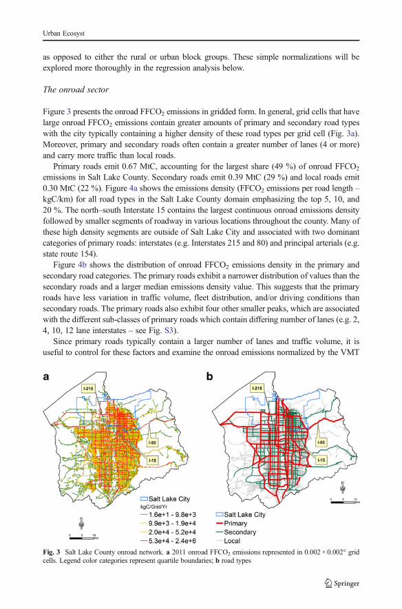
Figure 3 presents the onroad FFCO2 emissions in gridded form. In general, grid cells that havelarge onroad FFCO2 emissions contain greater amounts of primary and secondary road typeswith the city typically containing a higher density of these road types per grid cell (Fig. 3a).Moreover, primary and secondary roads often contain a greater number of lanes (4 or more)and carry more traffic than local roads.

Primary roads emit 0.67 MtC, accounting for the largest share (49 %) of onroad FFCO2

emissions in Salt Lake County. Secondary roads emit 0.39 MtC (29 %) and local roads emit0.30 MtC (22 %). Figure 4a shows the emissions density (FFCO2 emissions per road length –kgC/km) for all road types in the Salt Lake County domain emphasizing the top 5, 10, and20 %. The north–south Interstate 15 contains the largest continuous onroad emissions densityfollowed by smaller segments of roadway in various locations throughout the county. Many ofthese high density segments are outside of Salt Lake City and associated with two dominantcategories of primary roads: interstates (e.g. Interstates 215 and 80) and principal arterials (e.g.state route 154).

Figure 4b shows the distribution of onroad FFCO2 emissions density in the primary andsecondary road categories. The primary roads exhibit a narrower distribution of values than thesecondary roads and a larger median emissions density value. This suggests that the primaryroads have less variation in traffic volume, fleet distribution, and/or driving conditions thansecondary roads. The primary roads also exhibit four other smaller peaks, which are associatedwith the different sub-classes of primary roads which contain differing number of lanes (e.g. 2,4, 10, 12 lane interstates – see Fig. S3).

Since primary roads typically contain a larger number of lanes and traffic volume, it isuseful to control for these factors and examine the onroad emissions normalized by the VMT

Fig. 3 Salt Lake County onroad network. a 2011 onroad FFCO2 emissions represented in 0.002 × 0.002° gridcells. Legend color categories represent quartile boundaries; b road types

Urban Ecosyst

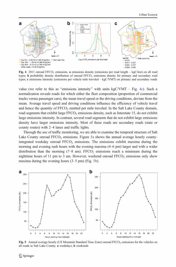
value (we refer to this as Bemissions intensity^ with units kgC/VMT – Fig. 4c). Such anormalization reveals roads for which either the fleet composition (proportion of commercialtrucks versus passenger cars), the mean travel speed or the driving conditions, deviate from themean. Average travel speed and driving conditions influence the efficiency of vehicle traveland hence the quantity of FFCO2 emitted per mile traveled. In the Salt Lake County domain,road segments that exhibit large FFCO2 emissions density, such as Interstate 15, do not exhibitlarge emissions intensity. In contrast, several road segments that do not exhibit large emissionsdensity have larger emissions intensity. Most of these roads are secondary roads (state orcounty routes) with 2–4 lanes and traffic lights.

Through the use of traffic monitoring, we are able to examine the temporal structure of SaltLake County onroad FFCO2 emissions. Figure 5a shows the annual average hourly county-integrated weekday onroad FFCO2 emissions. The emissions exhibit maxima during themorning and evening rush hours with the evening maxima (4–6 pm) larger and with a widerdistribution than the morning (7–8 am). FFCO2 emissions reach a minimum during thenighttime hours of 11 pm to 3 am. However, weekend onroad FFCO2 emissions only showmaxima during the evening hours (3–5 pm) (Fig. 5b).

Fig. 4 2011 onroad FFCO2 emissions. a emissions density (emissions per road length – kgC/km) on all roadtypes; b probability density distribution of onroad FFCO2 emissions density for primary and secondary roadtypes; c emissions intensity (emissions per vehicle mile traveled – kgC/VMT) on primary and secondary roads

Fig. 5 Annual average hourly (US Mountain Standard Time Zone) onroad FFCO2 emissions for the vehicles onall roads in Salt Lake County. a weekdays; b weekends

Urban Ecosyst

Figure 6 shows the same information but in a spatially explicit form (for the Salt Lake Citysub-domain). In general, larger FFCO2 are emitted on the primary and secondary roads at anygiven hour of a day. Emissions between 3 pm – 7 pm are the largest followed by between 9 am– 3 pm. These large emissions are found in the downtown and the eastern side of the city.FFCO2 emissions diminish after 9 pm.

Analysis

Residential FFCO2 drivers

The STIRPAT regression results applied to the residential FFCO2 emissions are presented inTable 3 (for descriptive statistics, correlation matrix, and spatial distribution maps, seesupplementary information, Tables S1-S6, Fig. S2). The adjusted R2 values range from 0.64to 0.78. Model 4 (census block groups within Salt Lake City) has the highest adjusted R2 valueof 0.78 while Model 3 (census block groups with lower mean income) has the lowest (0.64).

Fig. 6 Salt Lake City annual average hourly onroad FFCO2 emissions represented in 0.002× 0.002° grid cells.Emissions are represented as the deviation from the 24-h logged median value in five time bins

Urban Ecosyst

Across all of the models, the population variable is significant at the 0.01 % level andexhibits a weak sub-linear relationship suggesting that FFCO2 emissions increase in very nearlydirect proportion with population across census block groups, all else being equal. Populationhas the greatest proportional influence on the FFCO2 emissions among the independentvariables considered. When using only census block groups with a mean income in the lowestincome cohort, the relationship is more sub-linear, suggesting that a 1 % increase in populationacross low income census block groups is met with a 0.85 % increase in FFCO2 emissions.

Per capita income is the next most influential independent variable with coefficient valuesof approximately +0.6, except when subsetting by low-income where the coefficient is reducedto +0.3. This suggests that as income rises, FFCO2 emissions increase as well, though at a sub-linear rate, all else being equal. For census block groups with a lower mean per capita income,the influence of income is roughly half that of the general population. This suggests thatincrements of wealth among census block groups with higher mean per capita income lead togreater proportional increases in FFCO2 when compared to census block groups with lowermean income.

Housing units per capita exhibits a relationship to residential FFCO2 emissions across censusblock groups, though the importance varies quite a bit among the models. Household size (i.e.,number of people living in a housing unit), a more intuitive metric, is the reciprocal of housingunits per capita. For the county as a whole, there is a positive relationship between housing unitsper capita and FFCO2 emissions such that a 1 % decline in household size is associated with0.21 % rise in FFCO2 emissions, all else being equal. This suggests that block groups with agreater average number of individuals per household (but the same total block group popula-tion) have lower FFCO2 emissions though the decline is not directly proportional to householdsize, but sub-linear. The influence of household size is much more pronounced for city and lowincome residents than for the population as a whole with slope coefficients of +0.37 and +0.40for city and low income residents, respectively. This result suggests that if one were to comparetwo census block groups for which total population, total housing units, building age, andmeanper capita income were identical, the census block group with a greater average household size

Table 3 Regression model coefficients and statistics

Variables Model 1:County

Model 2:High Income

Model 3:Low Income

Model 4:City

Model 5:Outside City

Coeff SE Coeff SE Coeff SE Coeff SE Coeff SE

Intercept 0.46 0.42 1.19 0.99 4.43*** 1.03 1.37* 0.67 -0.47 0.53

Population (loge) 0.94*** 0.03 0.95*** 0.05 0.85*** 0.05 0.93*** 0.06 0.97*** 0.03

Housing units per capita (loge) 0.21*** 0.04 0.11 0.08 0.40*** 0.08 0.37*** 0.07 0.13* 0.06

Housing units per area (loge) -0.05*** 0.01 -0.03 0.02 -0.04* 0.02 -0.01 0.02 -0.06*** 0.01

Building age (loge) 0.17*** 0.03 0.14*** 0.05 0.14** 0.05 0.06 0.05 0.25*** 0.03

Income per capita (loge) 0.63*** 0.02 0.54*** 0.07 0.31*** 0.09 0.57*** 0.03 0.67*** 0.03

Adjusted R2 0.77 0.74 0.64 0.78 0.77

Degrees of freedom 604 146 147 135 463

Coeff coefficient, SE standard error

***p < 0.001

**p < 0.01

*p < 0.05

Urban Ecosyst

(more individuals per housing unit) would have lower FFCO2 emissions though not in directproportion to the difference in household size. The fact that this effect is more pronounced forcity block groups and those with a lower mean income may suggest that the efficiencies ofhousehold size are exploited to a greater degree in these subsets of the whole county domain.

A related variable, housing units per area, has little impact on FFCO2 emissions. Furthermore, thecoefficient for models 2 and 4 are not significant at the 0.05 level. Hence, for two census blockgroups in which per capita income, household size, building age, and population were identical, thecensus block group with the greater number of housing units would have smaller FFCO2 emissions,though the effect is barely discernable from zero. This suggests that, to the extent compactdevelopment has occurred within Salt Lake County, it has had little impact on FFCO2 emissions.

Building age shows a positive relationship with residential FFCO2 across all of the modelsas expected from the prior constraint on the NE-EUI with age. In general, older residentialbuildings are less energy-efficient due to older HVAC (heating, ventilation and air-conditioning) systems, less insulation, single-pane windows and leakier building envelopes.With the same demand and fuel composition, this will lead to greater FFCO2 emissions(Huang et al. 1991; Ewing and Rong 2008; DOE 2012). The dependence of FFCO2 emissionson building age show greater sensitivity when examining only census block groups outside thecity (slope coefficient of 0.25) versus those within (slope coefficient of 0.06). This is likely dueto the differing mix of building types within the city versus the county and the fact that eachbuilding type has a different ratio of old versus new NE-EUI values.

Onroad FFCO2 patterns

The road segments accounting for the top 20 % of the FFCO2 onroad emissions density, shownin Fig. 4a, can be explored in more detail in order to isolate spatio-temporal patterns andpotential policy options for FFCO2 emissions mitigation (Fig. 7). These road segments have

Fig. 7 Top 20 % of onroadFFCO2 emissions density andexisting public transit routes

Urban Ecosyst

emissions density values ranging from ~800 tC/km to ~5800 tC/km with interstates accountingfor the largest share (63 %), followed by secondary roads (23 %) and other primary roads(14 %) (Table 4).

We compare these dominant road segments with the existing public transit networks inorder to highlight potential policy opportunities aimed at lowering onroad FFCO2 emissions.Salt Lake County public transit includes bus, commuter rail, and light rail systems (Fig. 7). Busroutes are present throughout the county and provide service primarily on secondary roads.The bus routes are generally aligned with the road segments that have high emissions excepton State Route 154 (Fig. 7, insert map). The commuter and light rail networks, however, areless extensive and hence, could offer some policy options for onroad FFCO2 mitigation.Currently, both commuter and light rail (TRAX) systems provide services mainly along thecentral north–south corridor with less service along the east–west corridor. Hence, these east–west corridors that align with large onroad FFCO2 emissions may be candidates for optimallight rail expansion. Road corridors such as Interstate 215 and 80, and state route 154 arepossible targets. Were light rail expansion along these lines able to displace 25 % of theexisting traffic volume, this would mitigate ~50,000 tC/year, accounting for 8 % of the top20 % presented in Fig. 7 and Table 3. Using the current social cost of carbon (SCC) of $40/tonne of CO2 (EPA 2015), this equates to ~7 million dollars in carbon offset value.

Discussion

Salt Lake City has plans in place that include greenhouse gas reduction targets. For example,the BSalt Lake City Green: Energy and Transportation Sustainability Plan 2011^ aims toreduce greenhouse emissions to 17 % below 2005 levels by 2020 (Salt Lake City 2011).Likewise, the BSalt Lake City Sustainable Plan 2015^ sets environmental sustainability goalsthrough air quality improvement, energy use reduction, and zero-carbon transportation ser-vices. For example, the city aims to reduce total energy use in buildings by 5 % by the end of2015 through household solar energy and incentives to meet LEED building efficiencystandards. For the transportation sector, the city aims to reduce VMT by 6.5 %, increase cleanand alternative fuel vehicles to 15 % of the city fleet, extend the TRAX line, increase bikelanes by 50 %, and increase the efficiency of traffic flow via improved traffic-signal timing(Salt Lake City 2015). The FFCO2 analysis presented here may offer some specific guidanceon the operationalization of these goals.

Table 4 Statistical description of the road segments accounting for the top 20 % of FFCO2 onroad emissionsdensity

Road Type Total Road Length (km) Total Emissions (tC) Emissions density (tC/Km)

% total in parentheses Min Median Max

Primary 241 (66 %) 470,250 (77 %) 813 1453 5766

Interstates 154 (42 %) 384,037 (63 %) 1033 2336 5766

Other primary roads 87 (24 %) 86,213 (14 %) 813 960 1621

Secondary 127 (34 %) 137,812 (23 %) 806 1054 2802

Total 368 (100 %) 608,062 (100 %)

Urban Ecosyst

The residential sector

Quantification and analysis of residential buildings in Salt Lake County at fine space andtime scales offer greater insight into the drivers of emissions than can be gleaned fromzero-dimensional (i.e. simple pie-chart) representations of FFCO2 emissions. The spatialpattern of residential emissions, normalized by population or number of housing units(Figs. 1 and 2), suggests that mitigation might find efficiencies in application by knowingwhere FFCO2 emissions are largest and why. Simple normalization of the spatial FFCO2

emissions indicate that policies targeted to building envelopes versus occupant behaviorwould likely emphasize different geographies. For example, policy targeting behavioralchange may find the greatest gain in the eastern half of the county while policy targetingbuilding envelopes may be most effective targeting suburban pockets in the east andsouth portions of the county.

For a deeper and potentially more nuanced guide to climate mitigation policy options, theSTIRPAT regression results are informative. Of the variables considered here, FFCO2 emis-sions are most sensitive to population and per capita income. The proportional relationship topopulation begs comparison to recent work exploring scaling relationships between city sizeand a number of urban attributes (Bettencourt et al. 2007; Cottineau et al. 2015). Indeed recentwork examining FFCO2 emissions across cities of varying size remains unclear regardingwhether or not FFCO2 emissions scale sub-linearly or super-linearly with population (Fragkiaset al. 2013; Oliveira et al. 2014; Arcaute et al. 2015). The results presented here, albeit at thesub-city scale, suggest linear or very slightly sub-linear scaling. Perhaps most interesting is theshift in the linear relationship when the lowest income group is examined in isolation. In thelow-income block groups, FFCO2 emissions do not rise proportionally with population but at alessened rate (Table 3).

This is similar to the dynamics found in relation to per capita income, the other high-influence variable in the regression analysis. Wealthier census block groups show FFCO2

emissions with nearly twice (+0.54 versus +0.31) the sensitivity to per capita income than thelower income census block groups. This suggests a non-linear relationship between FFCO2

emissions and per capita income. Increasing increments of income in the higher income blockgroups are met with greater increases in FFCO2 emissions compared to the lower incomeblock groups, all else being equal. Though our data cannot precisely identify the dynamics atwork, we can speculate. Energy use behavior, lifestyle, and income expenditure preferencescould explain the emission differences between the high- and low-income block groups (Haaset al. 1998; Bin and Dowlatabadi 2005; Hubacek et al. 2007). For example, it is possible that inthe lower income block groups, households will allocate increases in income to other prioritycommodities such as food or clothing first, before allocation to greater energy demand forspace heating/cooling or water heating. Or additional increments in wealth among the lowerincome block groups correlate with improved housing with accompanying higher efficiencyspace heating/cooling systems. Hence, increased heating/cooling comfort is delivered withlittle change in energy requirements. Conversely, added increments of wealth among thehigher income block groups may correlate with larger homes with little heating/coolingequipment efficiency improvement as that home attribute is already saturated. Furthermore,there is evidence that high-income residents set thermostats during winter at a more desirablecomfort level given the greater amount of disposable income that can be devoted to energycosts in comparison to low-income residents (Hunt and Gidman 1982; Santamouris et al. 2007;Walker and Meier 2008).

Urban Ecosyst

From a policy perspective these results suggest that emissions reductions may find greatestefficacy among the high income census block groups. Furthermore, policies aimed at energycost savings via improved building envelope efficiency may not be the most effectivemodality. Rather, appeals to personal responsibility or enabling better feedback informationloops may offer advantages. An example of this is programs in some utility ratepayer serviceareas that offer performance comparisons of individual ratepayers with surrounding averagesthat are included in utility billing statements (Opower 2015; Asensio and Delmas 2015).Centralized online presentation of spatial maps like those described here, advertised by utilitiesor city and county government, may also be effective.

Our findings of a negative relationship between household size and FFCO2 emissions areconsistent with other studies where larger households likely benefit from economies of scaleassociated with space and energy use (e.g. Cole and Neumayer (2004), Druckman and Jackson(2008), Lin et al. (2013), Pachauri (2004)). Furthermore, as with per capita income, theinfluence is sensitive to wealth and geography. For example, FFCO2 emissions among lowincome block groups show nearly four times the sensitivity to household size than the high-income block groups. City versus non-city block groups show three times the sensitivity. Thissuggests that low income block group inhabitants avail of the efficiency gains of co-habitationto a much greater degree than inhabitants of high-income block groups. This could be thoughtof as high-income individuals having space/water heating energy use that is tied to individualneeds, regardless of the physical efficiency of co-habitation, whereas low-income individualshave space/water heating energy-use that is more tied to building infrastructure, allowingenergy use per person to decline as more individuals occupy a given structure.

Somewhat surprisingly, our results do not seem to support other research that finds loweremissions associated with compact development (Holden and Norland 2005; Norman et al.2006; Ewing and Rong 2008). Though the regression coefficient is negative (less FFCO2

emitted for greater housing density), the magnitude is consistently less than 0.1 across themodels. However, most of the density effect owes to onroad transportation reductions garneredwith greater housing density as opposed to building space/water heating, the primary source ofresidential building FFCO2 emissions in our production-based framework (Ewing et al. 2003;Glaeser and Kahn 2010).

The onroad sector

FFCO2 emissions density (emissions per road length) is a useful metric to identify the spatialdistribution of FFCO2 emissions for a road type across the landscape (Kinnee et al. 2004).Emissions intensity (emissions per vehicle mile travel), by contrast, provides insights on thedriving behavior, traffic conditions and fleet composition—elements affecting the fuel econ-omy (miles per gallon, mpg) and fuel efficiency of a vehicle (Mendoza et al. 2013). Analysisof the spatial distribution using emissions density and intensity metrics can be useful for policymakers to find the cost-effective solutions to alleviate onroad FFCO2 as this sector contributesto nearly half of the Salt Lake County FFCO2 emissions.

We find primary roads, especially some portions of the interstates, represent the largest 5 %of the emissions density (>0.22 MtC/km) in Salt Lake County (Fig. 4a). This is due to thenature of interstates which typically have greater traffic volumes and a greater number of lanes(usually 4 or more) compared to other road types. To assist with the 6.5 % reduction in VMToutlined in the Salt Lake City Sustainable Plan 2015, our results suggest that an effectivestrategy to mitigate FFCO2 emissions may be to target these high-emitting road segments first.

Urban Ecosyst

These roads already account for ~28 % of the Salt Lake County’s VMT and contribute to~20 % (~0.27 MtC) of the County’s total emissions.

When examining high-emitting road segments in relation to current public transportationsystems in Salt Lake County, we find opportunities for alignment with public transportationexpansion. These road segments account for nearly half of the county’s onroad FFCO2

emissions (Tables 2 and 4). Policies to reduce FFCO2 could consider expanding existingpublic transportation such as light rail or bus rapid transit (BRT) service to some of these roadsegments. All modes of public transportation including light rail, BRT and buses emit lessFFCO2 per passenger mile than private passenger cars (Vincent and Jerram 2006). Forinstance, O’Toole (2008) estimated the amount US average emissions per passenger mile as0.54 and 0.36 lb of FFCO2, respectively for passenger cars and light rail. Lochner (2013)estimated expansion of the light rail system (e.g. TRAX blue line) in the county wouldincrease ridership by at least 12,000-14,000 passengers per day. Lochner also estimated thatif the current light rail service was Bturned off^ for a day, 29,000 vehicles per day would beadded along the north–south corridors. Finally, a study by Ewing et al. (2014) showed that theextension of the TRAX red line serving the University of Utah campus reduced the number ofannual average daily traffic by at least 7500. This saves ~362,000 gal of gasoline and prevents~7 million pounds of FFCO2 from being emitted annually.

In contrast to the pattern associated with FFCO2 emissions density, road segments withhigh FFCO2 emission intensity (>28 grams/VMT) are found on primarily secondary roadsrather than primary roads (Fig. 4a). Secondary roads are designed for balancing betweentraffic mobility and land access with shorter distance and lower speed (up to 40 mph) bycollecting the traffic from local roads and connecting them with primary roads. Bycontrast, primary roads are designed to offer a higher degree of traffic mobility at thegreatest speed and for the longest uninterrupted distance (Federal Highway Administration2015). Vehicles traveling at an average speed below 40 mph are less fuel efficient (hence,emit more FFCO2) than when traveling at an average speed of 40–60 mph (Barth andBoriboonsomsin 2009).

Vehicles travelling on primary roads have a higher probability of maintaining a steadytravel speed compared to secondary roads where traffic lights and traffic congestion arecommon (Barth and Boriboonsomsin 2009). Traffic lights and traffic congestion areobstacles that requires vehicles to make more frequent stops as well as increase vehicleidling time, frequent acceleration and deceleration (i.e., Bstop-and-go^ traffic) leading topoor fuel economy and increased FFCO2 emissions per mile travelled. Hence, thefunctionality of the secondary roads suggests that lower traveling speed, traffic lights,and traffic congestions are drivers of the larger FFCO2 emissions intensity. One of thestrategies that will lower FFCO2 emissions on these types of roads is to reduce vehicleidling time and stop-and-go traffic through improved traffic-signal timing (Frey et al.2001; Madireddy et al. 2011). According to Koa Corporation (2011), improved traffic-signal timing in the Salt Lake City metropolitan area reduces average travel time by asmuch as 8 %, increases average speed by 8 %, decreases the number of stops by 17 %,and decreases fuel consumption by 5.9 %. Our results suggest that improving the traffic-signal timing where two high emission intensity road segments meet would yield thegreatest benefits to FFCO2 reduction on these secondary roads. Intersections where highemission intensity road segments meet account for ~46 % (or ~ 127,000 tC) of the FFCO2

emissions of the high emission intensity cohort identified in Fig. 4c (FFCO2/VMT>0.028). Using the estimated fuel consumption reduction value reported by Koa

Urban Ecosyst

Corporation of 5.9 %, this would potentially reduce the amount of FFCO2 by ~7500 tC.Using an SCC value of $40/tonnes of CO2 (EPA 2015), this equates to $1,097,334 incarbon offset value.

Conclusions

We have applied the Hestia FFCO2 emissions quantification approach to Salt Lake County inorder to demonstrate potential for greenhouse gas emissions mitigation policy guidance. Somedepartures from the previously described Hestia methodology were required due to advancesin data availability and idiosyncrasies associated with the Salt Lake spatial domain.

The initial breakdown of FFCO2 emissions shows the onroad FFCO2 emissions as thedominant sector (42.9 %) followed by the residential (20.8 %) and industrial (12.6 %) sectors.The residential and onroad emissions in the city are somewhat overrepresented relative topopulation proportions. This is particularly true for the commercial sector due to the impor-tance of the city as the commercial hub of the county.

Simple normalization of the residential emissions shows distinct spatial patterns with percapita emissions higher in the eastern half of the county but normalization per housing unitexhibiting a much more dispersed pattern consistent with suburban growth. We applied theSTIRPAT regression analysis to better understand the driving factors of the residential buildingFFCO2 emissions. At a scale of the census block group, population, per capita income,household size, and building age were found to have a statistically significant influence onFFCO2 emissions. However, housing density had little to no effect on FFCO2 emissions. Wefind that the level of influence of per capita income and household size on FFCO2 emissionsare themselves sensitive to per capita income. Increases in per capita income among highincome block groups shows almost twice the impact on FFCO2 emissions than the low incomeblock groups (+0.54 % versus +0.31 % rise in FFCO2 per 1 % rise in per capita income, allelse being equal). Increases in household size among low income block groups results innearly four times the impact on FFCO2 emissions compared to high income block groups(−0.40 % versus −0.11 % decline in FFCO2 per 1 % rise in household size, all else beingequal).

These results suggest that policies aimed at the residential sector may find greatest successif structured to target high-income groups through appeals to personal responsibility or viabetter information feedbacks (e.g. the Bdashboard effect^, neighborhood comparisons). Boththe per capita income and household size results suggest that the sensitivities relate less toinfrastructure and more to choice and lifestyle. Awareness of energy or emitting intensity maybe low among these groups or it may be triggered through simple outreach programs accessedto ratepayers through utility billing platforms.

Onroad emissions are dominated by the primary road category (49 %) followed bysecondary (29 %) and local roads (22 %). Primary road FFCO2 emissions exhibit a highermedian emissions density value with less variance in comparison to secondary roads. This islikely a result of the driving characteristics on primary roads where vehicles operate atconditions closer to optimal efficiency relative to the stop-and-go style driving typical onsecondary roads. As a result, secondary roads exhibit larger emissions intensity when com-pared to primary roads. We compare these high emitting road segments with existing publictransportation networks and find opportunities for extension of for example, the existing lightrail system. Doing so has the potential to offset approximately ~50,000 tC/year of FFCO2

Urban Ecosyst

emissions, which equates to ~ 7 million dollars. Improving the traffic-signal timing where highemissions intensity roads intersect could improve the traffic flow and reduce the overallFFCO2 emissions. Such improvements could potentially reduce the amount of FFCO2 by~7500 tC/year, equivalent to ~ $1 million in carbon offset value.

Our study has some caveats. The Hestia approach relies on a large and diverse suite of dataand modeling constructs. Among these, there is little accompanying uncertainty. In manycases, uncertainty is challenging to assign based on the nature of the incoming data. Hence, adevoted effort is needed to generate uncertainty and propagate those uncertainties through theHestia approach to provide an improved understanding of where results are more or lesscertain in space and time. This remains a high priority for future research.

There are a series of improvements that could be made to the underlying data sourcesthemselves. For example, greater accuracy in the individual building level FFCO2 emissionscould be generated with individual address-level utility billing. This would allow for a betterassignment of emissions to buildings with gas feeds versus those completely reliant uponelectricity and improve the estimation with directly metered gas amounts. Though attemptshave been made to acquire this data, there have been very few instances of success due to theconcern over the privacy of ratepayer data. But, there is no question that directly metered datais a critical need in Salt Lake City and across the United States. A system similar to that usedby health researchers when accessing individual health data is much needed and would providea profound change in the quality of data and the questions science could answer regardingenergy flows and carbon emissions.

Regarding the onroad FFCO2 estimation, traffic data outside of the city of Salt Lake domainis currently very limited. Hence, onroad emissions are supported by varying levels of qualityand further work could repair this disparity. Furthermore, data that provides a greater level ofdetail on vehicle type would improve emissions and allow for a better understanding of thedrivers of onroad FFCO2 emissions. Finally, the approach taken in the Hestia system isfocused on a Bproduction^ style estimate of FFCO2 emissions. Though a critical approachfor partnership with atmospheric measurements of CO2, this approach within the onroad sectorleaves little understanding of the driving forces behind emissions. The alternative, transporta-tion demand modeling, can solve this problem but relies on little empirical data. Combiningthe empirically-based approach used in Hestia with transportation demand modeling is apotentially powerful way to provide accurate space/time estimate of onroad emissions with alink to the socio-economic and engineering drivers. This combination would offer not onlydiagnostic but prognostic capability, sorely needed in efforts to mitigate onroad FFCO2

emissions in urban areas.

Acknowledgements This research was supported by grants from the Department of Energy DE-SC-001-0624,the National Science Foundation grant EF-01241286, National Institute of Standards and Technology grant70NANB14H321, and National Oceanic and Atmospheric Administration Climate Program Office’s Atmospher-ic Chemistry, Carbon Cycle, and Climate Program grant NA14OAR4310178. We also would like to thankJerome Zenger, Kevin Bell, and Semih Yildiz for assisting with the data collection and inquiry.

References

AirNav (2014) Airport information. http://www.airnav.com/. Accessed 9 Jan 2014Arcaute E, Hatna E, Ferguson P et al (2015) Constructing cities, deconstructing scaling laws. J R Soc Interface

12:20140745. doi:10.1098/rsif.2014.0745

Urban Ecosyst

Asefi-Najafabady S, Rayner PJ, Gurney KR, et al (2014) A multiyear, global gridded fossil fuel CO2 emission dataproduct: Evaluation and analysis of results. J Geophys Res Atmos 119:2013JD021296. doi: 10.1002/2013JD021296

Asensio OI, Delmas MA (2015) Nonprice incentives and energy conservation. Proc Natl Acad Sci 112:E510–E515. doi:10.1073/pnas.1401880112

Barth M, Boriboonsomsin K (2009) Traffic congestion and greenhouse gases. ACCESS Mag 1:1–9Bettencourt LMA, Lobo J, Helbing D et al (2007) Growth, innovation, scaling, and the pace of life in cities. Proc

Natl Acad Sci 104:7301–7306. doi:10.1073/pnas.0610172104Bin S, Dowlatabadi H (2005) Consumer lifestyle approach to US energy use and the related CO2 emissions.

Energ Policy 33:197–208. doi:10.1016/S0301-4215(03)00210-6Bréon FM, Broquet G, Puygrenier V et al (2015) An attempt at estimating Paris area CO2 emissions from

atmospheric concentrationmeasurements. Atmos ChemPhys 15:1707–1724. doi:10.5194/acp-15-1707-2015US Census Bureau (2015) State & County QuickFacts. http://www.census.gov/quickfacts/table/IPE120213/

49035,00. Accessed 7 Sep 2015Ciais P, Sabine C, Bala G et al (2013) Carbon and other biogeochemical cycles. In: Stocker TF, Qin D, Plattner

G-K et al (eds) Climate change 2013: the physical science basis. Contribution of Working Group I to theFifth Assessment Report of the Intergovernmental Panel on Climate Change. Cambridge University Press,Cambridge, pp 465–570

Cole MA, Neumayer E (2004) Examining the impact of demographic factors on air pollution. Popul Environ 26:5–21. doi:10.1023/B:POEN.0000039950.85422.eb

Collins M, Knutti R, Arblaster J et al (2013) Long-term climate change: projections, commitments andirreversibility. In: Stocker TF, Qin D, Plattner GK et al (eds) Climate change 2013: the physical sciencebasis. Contribution of Working Group I to the Fifth Assessment Report of the Intergovernmental Panel onClimate Change. Cambridge University Press, Cambridge, pp 1029–1136

Cottineau C, Hatna E, Arcaute E, Batty M (2015) Paradoxical interpretations of urban scaling laws. ArXiv E-Prints 1507:7878

Cox PM, Betts RA, Jones CD et al (2000) Acceleration of global warming due to carbon-cycle feedbacks in acoupled climate model. Nature 408:184–187. doi:10.1038/35041539

Dai A (2013) Increasing drought under global warming in observations and models. Nat Clim Chang 3:52–58.doi:10.1038/nclimate1633

Dietz T, Rosa EA (1997) Effects of population and affluence on CO2 emissions. Proc Natl Acad Sci 94:175–179Dodman D (2011) Forces driving urban greenhouse gas emissions. Curr Opin Environ Sustain 3:121–125. doi:

10.1016/j.cosust.2010.12.013DOE (2012) 2011 buildings energy data book. Office of Energy Efficiency and Renewable Energy, Department

of Energy, WashingtonDruckman A, Jackson T (2008) Household energy consumption in the UK: a highly geographically and socio-

economically disaggregated model. Energ Policy 36:3177–3192. doi:10.1016/j.enpol.2008.03.021Ehleringer JR, Schauer AJ, Lai C et al (2008) Long-term carbon dioxide monitoring in Salt Lake City. AGU Fall

Meet Abstr 43:0466Ehleringer J, Pataki DE, Lai C, Schauer A (2009) Long-term results from an urban CO2 monitoring network.

AGU Fall Meet Abstr 33:0414Ehrlich PR, Holdren JP (1971) Impact of population growthEIA (2002) Distillate fuel oil sales for railroad use. US Energy Information Administration, Department of

Energy. www.eia.gov/dnav/pet/pet_cons_821use_a_epd0_vrr_mgal_a.htm. Accessed 5 Jan 2002EIA (2013a) Fuel oil and kerosene sales. http://www.eia.gov/petroleum/fueloilkerosene/. Accessed 8 Jul 2013EIA (2013b) Refiner petroleum product prices by sales type. http://www.eia.gov/dnav/pet/pet_pri_refoth_a_

EPJK_PTG_dpgal_a.htm. Accessed 8 Jul 2013EPA (2015) Social Cost of Carbon. https://www3.epa.gov/climatechange/EPAactivities/economics/scc.html.

Accessed 30 Sep 2015EPA (2016) The 2011 National Emissions Inventory. http://www.epa.gov/ttnchie1/net/2011inventory.html.

Accessed 3 Mar 2016Ewing R, Rong F (2008) The impact of urban form on U.S. residential energy use. Hous Policy Debate 19:1–30.

doi:10.1080/10511482.2008.9521624Ewing R, Pendall R, Chen D (2003) Measuring sprawl and its transportation impacts. Transp Res Rec J Transp

Res Board 1831:175–183. doi:10.3141/1831-20Ewing R, Tian G, Spain A, Goates J (2014) Effects of light-rail transit on traffic in a travel corridor. J Public

Transp. doi:10.5038/2375-0901.17.4.6Fan Y, Liu L-C, Wu G, Wei Y-M (2006) Analyzing impact factors of CO2 emissions using the STIRPAT model.

Environ Impact Assess Rev 26:377–395. doi:10.1016/j.eiar.2005.11.007Federal Highway Administration (2014) Field manual. https://www.fhwa.dot.gov/policyinformation/hpms/

fieldmanual/chapter1.cfm. Accessed 11 Jul 2014

Urban Ecosyst

Federal Highway Administration (2015) Flexibility in highway design chapter 3: functional classification. http://www.fhwa.dot.gov/environment/publications/flexibility/ch03.cfm. Accessed 20 Sep 2015

Feng K, Hubacek K, Guan D (2009) Lifestyles, technology and CO2 emissions in China: a regional comparativeanalysis. Ecol Econ 69:145–154. doi:10.1016/j.ecolecon.2009.08.007

Fragkias M, Lobo J, Strumsky D, Seto KC (2013) Does size matter? Scaling of CO2 emissions and U.S. urbanareas. PLoS ONE 8:e64727. doi:10.1371/journal.pone.0064727

FreyHC, Rouphail NM,Unal A, Colyar JD (2001) Emissions reduction through better trafficmanagement: an empiricalevaluation based upon on-road measurements. CTE/NCDOT Joint Environmental Research Program, Raleigh

Gately CK, Hutyra LR,Wing IS (2015) Cities, traffic, and CO2: a multidecadal assessment of trends, drivers, andscaling relationships. Proc Natl Acad Sci 112:4999–5004. doi:10.1073/pnas.1421723112

Glaeser EL, Kahn ME (2010) The greenness of cities: carbon dioxide emissions and urban development. J UrbanEcon 67:404–418. doi:10.1016/j.jue.2009.11.006

Gomez-Ibanez DJ, Boarnet MG, Brake DR, et al (2009) Driving and the built environment: the effects of compactdevelopment on motorized travel, energy use, and CO2 emissions. Oak Ridge National Laboratory (ORNL)

Gurney KR, Law RM, Denning AS et al (2002) Towards robust regional estimates of CO2 sources and sinksusing atmospheric transport models. Nature 415:626–630. doi:10.1038/415626a

Gurney K, Ansley W, Mendoza D et al (2007) Research needs for finely resolved fossil carbon emissions. EOSTrans Am Geophys Union 88:542–543. doi:10.1029/2007EO490008

Gurney K, Mendoza D, Zhou Yet al (2009) High resolution fossil fuel combustion CO2 emission fluxes for theUnited States. Environ Sci Technol 43:5535–5541

Gurney KR, Razlivanov I, Song Yet al (2012) Quantification of fossil fuel CO2 emissions on the building/streetscale for a large U.S. City. Environ Sci Technol 46:12194–12202. doi:10.1021/es3011282

Haas R, Auer H, Biermayr P (1998) The impact of consumer behavior on residential energy demand for spaceheating. Energy Build 27:195–205. doi:10.1016/S0378-7788(97)00034-0

Heiple S, Sailor DJ (2008) Using building energy simulation and geospatial modeling techniques to determinehigh resolution building sector energy consumption profiles. Energy Build 40:1426–1436. doi:10.1016/j.enbuild.2008.01.005

Hojjati B, Wade SH (2012) U.S. household energy consumption and intensity trends: a decomposition approach.Energ Policy 48:304–314. doi:10.1016/j.enpol.2012.05.024

Holden E, Norland IT (2005) Three challenges for the compact city as a sustainable urban form: householdconsumption of energy and transport in eight residential areas in the greater Oslo region. Urban Stud 42:2145–2166. doi:10.1080/00420980500332064

Hsu A, Moffat AS, Weinfurter AJ, Schwartz JD (2015) Towards a new climate diplomacy. Nat Clim Chang 5:501–503. doi:10.1038/nclimate2594

Huang J, Akbari H, Rainer L, Ritschard R (1991) 481 prototypical commercial buildings for 20 urban marketareas. Lawrence Berkeley Laboratory, Berkeley

Hubacek K, Guan D, Barua A (2007) Changing lifestyles and consumption patterns in developing countries: ascenario analysis for China and India. Futures 39:1084–1096. doi:10.1016/j.futures.2007.03.010

Hunt DRG, Gidman MI (1982) A national field survey of house temperatures. Build Environ 17:107–124. doi:10.1016/0360-1323(82)90048-8

IEA (2008) World energy outlook. Head of communication and information. Office International Energy Agency(EIA), Paris

IEA (2009) Cities, towns & renewable energy: yes in my front yard. International Energy Agency (IEA), ParisJenks M, Burton E, Williams K (1996) Compact cities and sustainability: an introduction. In: Jenks M, Burton E,

Williams K (eds) The compact city: a sustainable urban form? E & FN Spon. Chapman & Hall, LondonKennedy C, Steinberger J, Gasson B et al (2009) Greenhouse gas emissions from global cities. Environ Sci

Technol 43:7297–7302. doi:10.1021/es900213pKinnee EJ, Touma JS, Mason R et al (2004) Allocation of onroad mobile emissions to road segments for air

toxics modeling in an urban area. Transp Res Part Transp Environ 9:139–150. doi:10.1016/j.trd.2003.09.003Koa Corporation (2011) Traffic signal management and synchronization project city of Salt Lake City. Koa

Corporation, Orange, CALankao PR, Tribbia JL, Nychka D (2009) Testing theories to explore the drivers of cities’ atmospheric emissions.

Ambio 38:236–244Lauvaux T, Pannekoucke O, Sarrat C et al (2009) Structure of the transport uncertainty in mesoscale inversions of

CO2sources and sinks using ensemble model simulations. Biogeosciences 6:1089–1102Lauvaux T, Miles NL, Deng A, et al. (2016) High resolution atmospheric inversion of urban CO2 emissions

during the dormant season of the Indianapolis Flux Experiment (INFLUX). (minor revision in AtmosphericChemistry and Physics)

Lin T, Yu Y, Bai X et al (2013) Greenhouse gas emissions accounting of urban residential consumption: ahousehold survey based approach. PLoS ONE 8, e55642. doi:10.1371/journal.pone.0055642

Urban Ecosyst

Lochner (2013) UTA network study: next tier program final report. Lochner, Salt Lake CityMadireddy M, De Coensel B, Can A et al (2011) Assessment of the impact of speed limit reduction and traffic

signal coordination on vehicle emissions using an integrated approach. Transp Res Part Transp Environ 16:504–508. doi:10.1016/j.trd.2011.06.001

McKain K, Wofsy SC, Nehrkorn T et al (2012) Assessment of ground-based atmospheric observations forverification of greenhouse gas emissions from an urban region. Proc Natl Acad Sci 109:8423–8428. doi:10.1073/pnas.1116645109

Meehl GA, Washington WM, Collins WD et al (2005) How much more global warming and sea level rise?Science 307:1769–1772. doi:10.1126/science.1106663

Mendoza D, Gurney KR, Geethakumar S et al (2013) Implications of uncertainty on regional CO2 mitigationpolicies for the U.S. onroad sector based on a high-resolution emissions estimate. Energ Policy 55:386–395.doi:10.1016/j.enpol.2012.12.027

Newman DP, Kenworthy JR (1989) Cities and automobile dependence: a sourcebook. Gower Publishing,Brookfield

Norman J, MacLean H, Kennedy C (2006) Comparing high and low residential density: life-cycle analysis ofenergy use and greenhouse gas emissions. J Urban Plan Dev 132:10–21. doi:10.1061/(ASCE)0733-9488(2006)132:1(10)

NRC (2010) Verifying greenhouse gas emissions: methods to support international climate agreements. NationalResearch Council (NRC). The National Academies Press, Washington

O’Toole R (2008) Does rail transit save energy or reduce greenhouse gas emissions? Cato Policy Anal 615:1–24Oliveira EA, Andrade JS, Makse HA (2014) Large cities are less green. Sci Rep. doi:10.1038/srep04235Olivier JG, Janssens-Maenhout G, Muntean M, Peters J (2014) Trends in global CO2 emissions: 2014 report.

JBL/JRC, The HagueOpower (2015) OPOWER. https://opower.com/. Accessed 17 Oct 2015Pachauri S (2004) An analysis of cross-sectional variations in total household energy requirements in India using

micro survey data. Energy Policy 32:1723–1735. doi:10.1016/S0301-4215(03)00162-9Pataki DE, Bowling DR, Ehleringer JR, Zobitz JM (2006) High resolution atmospheric monitoring of urban

carbon dioxide sources. Geophys Res Lett 33, L03813. doi:10.1029/2005GL024822Pataki DE, Xu T, Luo YQ, Ehleringer JR (2007) Inferring biogenic and anthropogenic carbon dioxide sources

across an urban to rural gradient. Oecologia 152:307–322. doi:10.1007/s00442-006-0656-0Pataki DE, Emmi PC, Forster CB et al (2009) An integrated approach to improving fossil fuel emissions

scenarios with urban ecosystem studies. Ecol Complex 6:1–14. doi:10.1016/j.ecocom.2008.09.003Petit JR, Jouzel J, Raynaud D et al (1999) Climate and atmospheric history of the past 420,000 years from the

Vostok ice core, Antarctica. Nature 399:429–436. doi:10.1038/20859Polyakov IV, Timokhov LA, Alexeev VA et al (2010) Arctic Ocean warming contributes to reduced polar ice

cap. J Phys Oceanogr 40:2743–2756. doi:10.1175/2010JPO4339.1Poumanyvong P, Kaneko S (2010) Does urbanization lead to less energy use and lower CO2 emissions? A cross-

country analysis. Ecol Econ 70:434–444. doi:10.1016/j.ecolecon.2010.09.029Rahmstorf S (2007) A semi-empirical approach to projecting future sea-level rise. Science 315:368–370. doi:10.

1126/science.1135456Rao P, Gurney K, Patarasuk R, et al. (2016) Spatio-temporal variations in onroad vehicle fossil fuel CO2

emissions in the Los Angeles Megacity (submitting to Environmental Polllution).Rayner PJ, Raupach MR, Paget M et al (2010) A new global gridded data set of CO2 emissions from fossil fuel

combustion: methodology and evaluation. J Geophys Res Atmos 115, D19306. doi:10.1029/2009JD013439Rignot E, Velicogna I, van den Broeke MR et al (2011) Acceleration of the contribution of the Greenland and

Antarctic ice sheets to sea level rise. Geophys Res Lett 38, L05503. doi:10.1029/2011GL046583RITA (2012) National transportation atlas database. Bureau of Transportation Statistics, US Department of

Transportation.Research and Innovative Technology Administration (RITA). http://www.rita.dot.gov/bts/sites/rita.dot.gov.bts/files/publications/national_transportation_atlas_database/index.html. Accessed 11 Jul2012

Salt Lake City (2010) Salt Lake City: community carbon footprint. Salt Lake City, UTSalt Lake City (2011) Salt Lake City green: energy and transportation sustainability plan. Salt Lake City, UTSalt Lake City (2014) Plan Salt Lake: Existing conditions report. Salt Lake City, UTSalt Lake City (2015) Sustainable Salt Lake 2015. Salt Lake City, UTSalt Lake City Transportation Division (2013) Salt Lake City Traffic Studies (ESRI Geodatabase). Data provided

by Salt Lake City Department of Information Management Services on 22 July 2013Salt Lake County Assessor’s Office (2013) Salt Lake County parcel data (ESRI Shapefile). Salt Lake County, UTSantamouris M, Kapsis K, Korres D et al (2007) On the relation between the energy and social characteristics of

the residential sector. Energy Build 39:893–905. doi:10.1016/j.enbuild.2006.11.001

Urban Ecosyst

Schuur EAG, Bockheim J, Canadell JG et al (2008) Vulnerability of permafrost carbon to climate change:implications for the global carbon cycle. Bioscience 58:701–714. doi:10.1641/B580807

Seto KC, Fragkias M, Güneralp B, Reilly MK (2011) A meta-analysis of global urban land expansion. PLoSONE 6, e23777. doi:10.1371/journal.pone.0023777

Seto KC, Güneralp B, Hutyra LR (2012) Global forecasts of urban expansion to 2030 and direct impacts onbiodiversity and carbon pools. Proc Natl Acad Sci 109:16083–16088. doi:10.1073/pnas.1211658109

Seto KC, Dhakal S, Bigio A et al (2014) Human settlements, infrastructure and spatial planning. In: Edenhofer O,Pichs-Madruga R, Sokona Yet al (eds) Climate change 2014: mitigation of climate change. Contribution ofWorking Group III to the Fifth Assessment Report of the Intergovernmental Panel on Climate Change.Cambridge University Press, Cambridge

Shakun JD, Clark PU, He F et al (2012) Global warming preceded by increasing carbon dioxide concentrationsduring the last deglaciation. Nature 484:49–54. doi:10.1038/nature10915

Smeds J, Wall M (2007) Enhanced energy conservation in houses through high performance design. EnergyBuild 39:273–278. doi:10.1016/j.enbuild.2006.07.003

Solomon S, Plattner G-K, Knutti R, Friedlingstein P (2009) Irreversible climate change due to carbon dioxideemissions. Proc Natl Acad Sci 106:1704–1709. doi:10.1073/pnas.0812721106

Stephens BB, Gurney KR, Tans PP et al (2007) Weak northern and strong tropical land carbon uptake fromvertical profiles of atmospheric CO2. Science 316:1732–1735. doi:10.1126/science.1137004

Strong C, Stwertka C, Bowling DR et al (2011) Urban carbon dioxide cycles within the Salt Lake Valley: amultiple-box model validated by observations. J Geophys Res Atmos 116, D15307. doi:10.1029/2011JD015693

Trenberth (2011) Changes in precipitation with climate change. Clim Res 47:123–138Turnbull JC, Sweeney C, Karion A et al (2015) Toward quantification and source sector identification of fossil

fuel CO2 emissions from an urban area: results from the INFLUX experiment. J Geophys Res Atmos 120:292–312. doi:10.1002/2014JD022555

UNFCCC (2015) Greenhouse Gas Inventory Data. http://unfccc.int/ghg_data/items/3800.phpVincent W, Jerram L (2006) The potential for bus rapid transit to reduce transportation-related CO2 emissions. J

Public Transp. doi:10.5038/2375-0901.9.3.12Walker IS, Meier AK (2008) Residential thermostats: comfort controls in California Homes. Lawrence Berkeley

National Laboratory, BerkeleyWang R, Tao S, Ciais P et al (2013) High-resolution mapping of combustion processes and implications for CO2

emissions. Atmos Chem Phys 13:5189–5203. doi:10.5194/acp-13-5189-2013Wheeler SM (2008) State and municipal climate change plans: the first generation. J Am Plan Assoc 74:481–

496. doi:10.1080/01944360802377973WWF, ICLEI (2015) Measuring up 2015: how local leadership can accelerate national climate goals. World

Wildlife Fund (WWF), Local Governments for Sustainability (ICLEI) USA, WashingtonYork R, Rosa EA, Dietz T (2003) STIRPAT, IPATand ImPACT: analytic tools for unpacking the driving forces of

environmental impacts. Ecol Econ 46:351–365. doi:10.1016/S0921-8009(03)00188-5Zhao Y, Nielsen CP, McElroy MB (2012) China’s CO2 emissions estimated from the bottom up: recent trends,

spatial distributions, and quantification of uncertainties. Atmos Environ 59:214–223. doi:10.1016/j.atmosenv.2012.05.027

Zheng S, Wang R, Glaeser EL, Kahn ME (2010) The greenness of China: household carbon dioxide emissionsand urban development. J Econ Geogr lbq031. doi: 10.1093/jeg/lbq031

Zhou Y, Gurney K (2010) A new methodology for quantifying on-site residential and commercial fossil fuel CO2emissions at the building spatial scale and hourly time scale. Carbon Manag 1:45–56. doi:10.4155/cmt.10.7

Urban Ecosyst