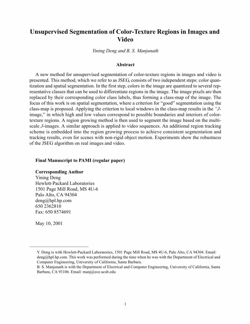
Unsupervised Segmentation of Color-Texture Regions in Images and Video

Yining Deng and B. S. Manjunath

Abstract

A new method for unsupervised segmentation of color-texture regions in images and video ispresented. This method, which we refer to as JSEG, consists of two independent steps: color quan-tization and spatial segmentation. In the first step, colors in the image are quantized to several rep-resentative classes that can be used to differentiate regions in the image. The image pixels are thenreplaced by their corresponding color class labels, thus forming a class-map of the image. Thefocus of this work is on spatial segmentation, where a criterion for “good” segmentation using theclass-map is proposed. Applying the criterion to local windows in the class-map results in the “J-image,” in which high and low values correspond to possible boundaries and interiors of color-texture regions. A region growing method is then used to segment the image based on the multi-scale J-images. A similar approach is applied to video sequences. An additional region trackingscheme is embedded into the region growing process to achieve consistent segmentation andtracking results, even for scenes with non-rigid object motion. Experiments show the robustnessof the JSEG algorithm on real images and video.

Final Manuscript to PAMI (regular paper)

Corresponding AuthorYining DengHewlett-Packard Laboratories1501 Page Mill Road, MS 4U-6Palo Alto, CA 94304deng@hpl.hp.com650 2362810Fax: 650 8574691

May 10, 2001

1

Y. Deng is with Hewlett-Packard Laboratories, 1501 Page Mill Road, MS 4U-6, Palo Alto, CA 94304. Email: deng@hpl.hp.com. This work was performed during the time when he was with the Department of Electrical and Computer Engineering, University of California, Santa Barbara. B. S. Manjunath is with the Department of Electrical and Computer Engineering, University of California, Santa Barbara, CA 93106. Email: manj@ece.ucsb.edu

1. Introduction

Image and video segmentation is useful in many applications for identifying regions of interest

in a scene or annotating the data. The MPEG-4 standard needs segmentation for object based

video coding. However, the problem of unsupervised segmentation is ill-defined because seman-

tic objects do not usually correspond to homogeneous spatio-temporal regions in color, texture, or

motion. Some of the recent work in image segmentation include stochastic model based

approaches [1], [6], [13], [17], [24], [25], morphological watershed based region growing [18],

energy diffusion [14], and graph partitioning [20]. The work on video segmentation include

motion based segmentation [3], [19], [21], [23], spatial segmentation and motion tracking [8],

[22], moving objects extraction [12], [15], and region growing using spatio-temporal similarity

[4], [16]. Quantitative evaluation methods have also been suggested [2].

Many of the existing segmentation techniques, such as direct clustering methods in color space

[5] and [9], work well on homogeneous color regions. Natural scenes are rich in color and texture.

Many texture segmentation algorithms require the estimation of texture model parameters.

Parameter estimation is a difficult problem and often requires good homogeneous region for

robust estimation. The goal of this work is to segment images and video into homogeneous color-

texture regions. A new approach called JSEG is proposed towards this goal. This approach does

not attempt to estimate a specific model for a texture region. Instead, it tests for the homogeneity

of a given color-texture pattern, which is computationally more feasible than model parameter

estimation.

In order to identify this homogeneity, the following assumptions about the image are made:

• Each image contains a set of approximately homogeneous color-texture regions. This assump-

tion conforms with our segmentation objective.

• The color information in each image region can be represented by a set of few quantized col-

ors. In our experience with a large number of different image datasets, including thousands of

images from the Corel stock photo gallery, we have found that this assumption is generally

valid.

2

• The colors between two neighboring regions are distinguishable -- a basic assumption in any

color image segmentation algorithm.

The basic idea of the JSEG method is to separate the segmentation process into two stages,

color quantization and spatial segmentation. In the first stage, colors in the image are quantized to

several representative classes that can be used to differentiate regions in the image. This quantiza-

tion is performed in the color space without considering the spatial distributions of the colors.

Then the image pixel values are replaced by their corresponding color class labels, thus forming a

class-map of the image. The class-map can be viewed as a special kind of texture composition. In

the second stage, spatial segmentation is performed directly on this class-map without considering

the corresponding pixel color similarity. The benefit of this two-stage separation is clear. It is a

difficult task to analyze the similarity of the colors and their distributions at the same time. The

decoupling of color similarity from spatial distribution allows development of more tractable

algorithms for each of the two processing stages. In fact, many good color quantization algo-

rithms exist and one of them [9] has been used in this work .

The main focus of this work is on spatial segmentation and the contributions can be summa-

rized as:

• We introduce a new criterion for image segmentation (Section 2). This criterion involves min-

imizing a cost associated with the partitioning of the image based on pixel labels.

• A practical algorithm is suggested towards achieving this segmentation objective. The notion

of “J-images” is introduced in Section 2. J-images correspond to measurements of local

homogeneities at different scales, which can indicate potential boundary locations.

• A spatial segmentation algorithm is then described in Section 3, which grows regions from

seed areas of the J-images to achieve the final segmentation.

Fig. 1 shows a schematic of the JSEG algorithm for color image segmentation. Extensions to

video segmentation are discussed in Section 4. We conclude with experimental results and discus-

sions in Section 5.

3

2. A Criterion for “Good” Segmentation

Typical 24-bit color images have thousands of colors, which are difficult to handle directly. In

the first stage of JSEG, colors in the image are coarsely quantized without significantly degrading

the color quality. The purpose is to extract only a few representative colors that can differentiate

neighboring regions in the image. Typically, 10-20 colors are needed in the images of natural

scenes. A good color quantization is important to the segmentation process. An unsupervised

color quantization algorithm based on human perception [9] is used in our implementation. This

quantization method is summarized in Appendix A. We will discuss the sensitivity to quantization

parameter selection later in Section 5.

Following quantization, the quantized colors are assigned labels. A color class is the set of

image pixels quantized to the same color. The image pixel colors are replaced by their corre-

sponding color class labels. The newly constructed image of labels is called a class-map. Exam-

ples of a class-map are shown in Fig. 2, where label values are represented by three symbols, ‘*’,

‘+’, and ‘o’. Usually, each image region contains pixels from a small subset of the color classes

and each class is distributed in a few image regions.

The class-map image can be viewed as a special kind of texture composition. The value of

each point in the class-map is the image pixel position, a 2-D vector (x, y). Each point belongs to

a color class. In the following, a criterion for “good” segmentation using these spatial data points

is proposed.

Let Z be the set of all N data points in a class-map. Let , , and m be the mean,

(1)

Suppose Z is classified into C classes, Zi, . Let mi be the mean of the Ni data points of

class Zi,

(2)

z x y,( )= z Z∈

m 1N---- z

z Z∈∑=

i 1 … C, ,=

mi1Ni----- z

z Zi∈∑=

4

Let

(3)

and

(4)

SW is the total variance of points belonging to the same class. Define

(5)

For the case of an image consisting of several homogeneous color regions, the color classes are

more separated from each other and the value of J is large. An example of such a class-map is

class-map 1 in Fig. 2 and the corresponding J value is 1.720. On the other hand, if all color classes

are uniformly distributed over the entire image, the value of J tends to be small. This is illustrated

by class-map 2 in Fig. 2 for which J equals 0. Fig. 2 shows another example of a three class distri-

bution for which J is 0.855, indicating a more homogeneous distribution than class-map 1. Notice

that there are three classes in each map and the number of points in each class is same for all three

maps. The motivation for the definition of J comes from the Fisher’s multi-class linear discrimi-

nant [10], but for arbitrary nonlinear class distributions. Note that in defining J we assume the

knowledge of class labels, whereas the objective in the Fisher’s discriminant is to find the class

labels.

Consider class-map 1 from Fig. 2. A “good” segmentation for this case would be three regions

each containing a single class of data points. Class-map 2 is uniform by itself and no segmentation

is needed. For class-map 3, a “good” segmentation would be two regions. One region contains

class ‘+’ and the other one contains classes ‘*’ and ‘o’. Fig. 3 shows the manual segmentation

results of class-map 1 and 3.

Now let us recalculate J over each segmented region instead of the entire class-map and define

the average by

ST z m– 2

z Z∈∑=

SW Si

i 1=

C

∑ z mi– 2

z Zi∈∑

i 1=

C

∑= =

J ST SW–( ) S⁄ W=

J

5

(6)

where Jk is J calculated over region k, Mk is the number of points in region k, N is the total number

of points in the class-map, and the summation is over all the regions in the class-map.

We now propose as the criterion to be minimized over all possible ways of segmenting the

image given the number of regions. For a fixed number of regions, a “better” segmentation tends

to have a lower value of . If the segmentation is good, each segmented region contains a few

uniformly distributed color class labels and the resulting J value for that region is small. There-

fore, the overall is also small. Notice that the minimum value can take is 0. The values of

calculated for class-map 1 and 3 are shown in Fig. 3. For the case of class-map 1, the partitioning

shown is optimal ( ).

3. A Spatial Segmentation Algorithm

The global minimization of for the entire image is not practical because there are millions of

ways to segment the image. However, observe that J, if applied to a local area of the class-map, is

also a good indicator of whether that area is in the region interiors or near region boundaries. We

can now think of constructing an image whose pixel values correspond to these J values calcu-

lated over small windows centered at the pixels. For convenience, we refer to these images as J-

images and the corresponding pixel values as local J values. The higher the local J value is, the

more likely that the corresponding pixel is near a region boundary. The J-image is like a 3-D ter-

rain map containing valleys and hills that actually represent the region interiors and region bound-

aries, respectively.

The size of the local window determines the size of image regions that can be detected. Win-

dows of small size are useful in localizing the intensity/color edges, while large windows are use-

ful for detecting texture boundaries. Often, multiple scales are needed to segment an image. In our

implementation, the basic window at the smallest scale is a 9 x 9 window without corners, as

shown in Fig. 4 (a). The corners are removed to make the window circular. The smallest scale is

J 1N---- MkJk

k∑=

J

J

J J J

J 0=

J

6

denoted as scale 1. From scale 1, the window size is doubled each time to obtain the next larger

scale. For computational reasons, successive windows are downsampled appropriately. Fig. 4 (b)

shows the window at scale 2, where the sampling rate is 1 out of 2 pixels along both x and y direc-

tions.

The characteristics of the J-images allow us to use a region-growing method to segment the

image. Consider the original image as one initial region. The algorithm starts the segmentation of

the image at a coarse initial scale. It then repeats the same process on the newly segmented

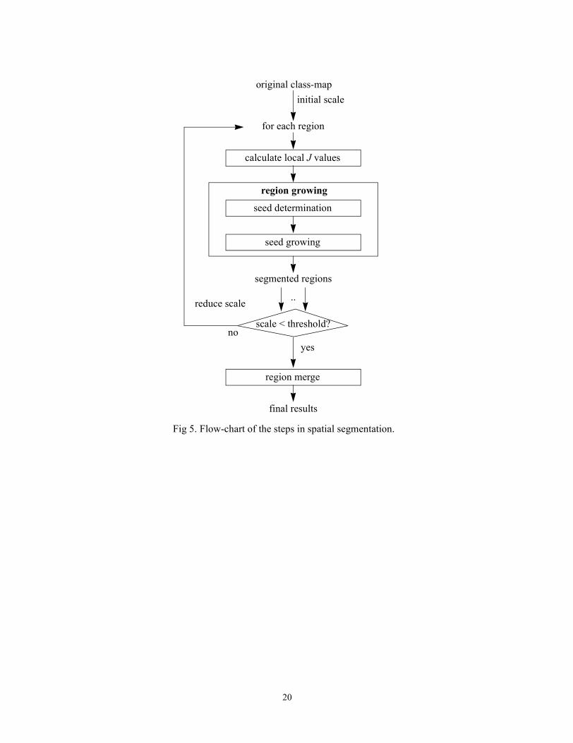
regions at the next finer scale. Fig. 5 shows a flow-chart of the steps in our spatial segmentation

algorithm. Region growing consists of determining the seed points and growing from those seed

locations. Region growing is followed by a region merging operation to give the final segmented

image. The user specifies the number of scales needed for the image, which affects how detail the

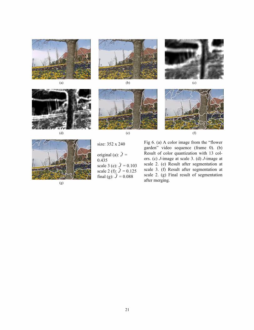
segmentation will be. Fig. 6 (a) shows a color image from the “flower garden” video sequence

(frame 0). The J-images at scale 3 and 2 are shown in Fig. 6(c) and Fig. 6(d), respectively.

3.1 Seed Determination

A set of initial seed areas are determined to be the basis for region growing. These areas corre-

spond to minima of local J values. In general, finding the best set of seed areas is a non-trivial

problem. The following simple heuristics have provided good results in the experiments:

1. Calculate the average and the standard deviation of the local J values in the region, denoted by

and respectively.

2. Set a threshold TJ at

(7)

a is chosen from several preset values that will result in the most number of seeds. Pixels with

local J values less than TJ are considered as candidate seed points. Connect the candidate seed

points based on the 4-connectivity and obtain candidate seed areas.

3. If a candidate seed area has a size larger than the minimum size listed in Table 1 at the corre-

sponding scale, it is determined to be a seed.

µJ σJ

TJ µJ aσJ+=

7

3.2 Seed Growing

The new regions are then grown from the seeds. It is slow to grow the seeds pixel by pixel. A

faster approach is used in the implementation:

1. Remove “holes” in the seeds.

2. Average the local J values in the remaining unsegmented part of the region and connect pixels

below the average to form growing areas. If a growing area is adjacent to one and only one

seed, it is assigned to that seed.

3. Calculate local J values for the remaining pixels at the next smaller scale to more accurately

locate the boundaries. Repeat Step 2.

4. Grow the remaining pixels one by one at the smallest scale. Unclassified pixels at the seed

boundaries are stored in a buffer. Each time, the pixel with the minimum local J value is

assigned to its adjacent seed and the buffer is updated until all the pixels are classified.

3.3 Region Merge

Region growing results in an initial segmentation of the image. It often has over-segmented

regions. These regions are merged based on their color similarity. The region color information is

characterized by its color histogram. The quantized colors from the color quantization process are

used as color histogram bins. The color histogram for each region is extracted and the distance

between two color histograms i and j is calculated by:

(8)

where P denotes the color histogram vector. The use of Euclidean distance is justified because the

colors are very coarsely quantized and there is little correlation between two color histogram bins.

The perceptually uniform CIE LUV color space is used.

An agglomerative method [10] is used to merge the regions. First, distances between the color

histograms of any two neighboring regions are calculated and stored in a distance table. The pair

of regions with the minimum distance are merged together. The color feature vector for the new

region is calculated and the distance table is updated along with the neighboring relationships.

DCH i j,( ) Pi Pj–=

8

The process continues until a maximum threshold for the distance is reached.

4. Spatio-temporal Segmentation and Tracking

The JSEG method can be modified to segment color-texture regions in video data. Here, our

approach differs from existing techniques in that it does not estimate exact object motion. Com-

mon approaches involve estimation of motion vectors, whether based on optical flow or affine

motion matching [3], [19], [22]. Following are some of the common problems associated with

motion estimation:

• Dense field motion vectors are not very reliable for noisy data.

• Affine transform is often inadequate to model the motion in close-up shots, especially when

objects are turning away from the camera.

• Occluded and uncovered areas introduce errors in estimation.

These are difficult problems and there are no good general solutions at present. Motion estima-

tion is very useful for coding to reduce the redundancies across video frames. On the other hand,

from a segmentation perspective, an accurate motion estimation is helpful but not necessary. This

work offers an alternative approach that does not estimate the exact motion vectors. Rather, object

movements are used as implicit constraints in the segmentation and tracking process, as explained

below. As a result, the proposed approach is more robust to non-rigid body motion.

In the following, we assume that the video data have been parsed into shots. Within each shot

the video scene is continuous and there are no abrupt changes. In the implementation, the method

described in [7] is used for the video shot detection.

4.1 Basic Scheme

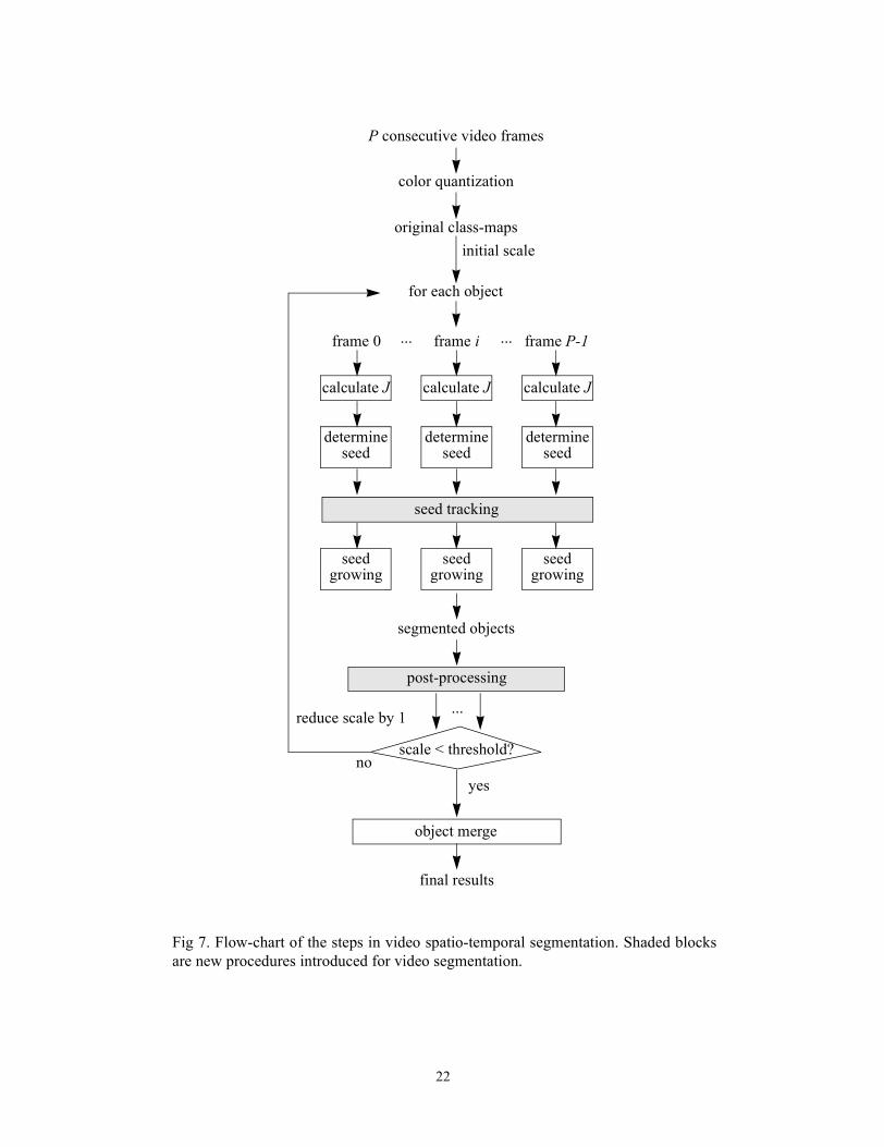
A schematic of the proposed approach is shown in Fig. 7. The goal is to decompose the video

into a set of objects in the spatio-temporal domain. Each object contains a homogenous color-tex-

ture pattern. It can be seen that the overall approach for each video frame is similar to the image

segmentation work with the exception of seed tracking and post-processing procedures. Seed

9

tracking will be explained in detail later. Post-processing smooths region boundaries. Since the

majority of computational time results from J value calculation and seed growing, the complexity

of the algorithm per frame is approximately the same as the one in image segmentation despite the

added computations.

The segmentation is performed on a group of consecutive frames. The number of frames P in

each group can be set equal to the video shot length, typically around 100 frames on the average.

Pixels in these frames are used for color quantization, where spatial and temporal information is

discarded in this process. After quantization, a color codebook is generated and the class-maps are

obtained by assigning pixels to their color classes using this codebook.

4.2 Seed Tracking

For the tracking method to work, object motion is assumed to be small with respect to its size.

In other words, there is a significant overlap between the object in two consecutive frames. If two

regions in adjacent frames have similar color-texture patterns and share partially the same spatial

locations, they are considered to be the same object. (We use the term object to refer to homoge-

neous image regions being tracked.)

Seed tracking is performed after seed determination, during which a set of region centers are

obtained. Note that in contrast to the region seeds in the traditional watershed approaches [18],

these seeds can be quite large, ranging from 1/3 to 2/3 of the region sizes. These seeds are tracked

together using the following procedure:

1. The seeds in the first frame are assigned as initial objects.

2. For each seed in the current frame:

If it overlaps with an object from the previous frame, it is assigned to that object;

Else a new object is created starting from this seed.

3. If a seed overlaps with more than one object, these objects are merged.

4. Repeat step 2 and 3 for all the frames in the group.

5. A minimum time duration is set for the objects. Very short-length objects are discarded.

10

Sometimes, false merges occur when two seeds of neighboring regions overlap with each other

across the frames due to object motion. To address this problem, let us first consider the overlap-

ping at the pixel level. For two pixels at the same spatial location but in two consecutive frames, a

modified measure J can be used to detect if their local neighbors have similar color distributions.

This new measure is denoted Jt and defined along the temporal dimension in a similar manner as

(1) to (5). Let Z be the set of N points in the local spatial windows centered on these two pixels.

Let tz be the relative temporal position of point z, , and since there are only two

frames involved. Let m be the mean of tz of all the N points. Since the number of points in each

frame is equal, m = 0.5. Again Z is classified into C color classes, Zi, . Let mi be the

mean of tz of the Ni data points of class Zi,

(9)

Let

(10)

and

(11)

The measure Jt is defined as

(12)

When a region and its surroundings are static, the Jt values are small for all the points. When a

region undergoes motion, the Jt value will become large when two points at the same spatial loca-

tions in the two frames do not belong to the same region. This often happens at region boundaries.

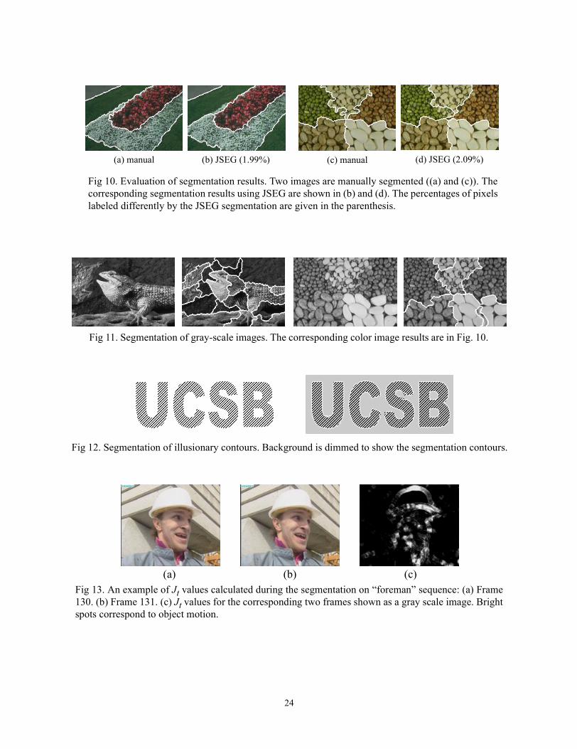
Fig. 13 shows an example of Jt values calculated during the segmentation on the “foreman”

sequence, where brighter pixels correspond to higher Jt values.

Jt is calculated for each point in the seeds. A threshold is set such that only points with small Jt

z Z∈ tz 0 1,{ }∈

i 1 … C, ,=

mi1Ni----- tz

z Zi∈∑=

ST tz m– 2

z Z∈∑=

SW Si

i 1=

C

∑ tz mi– 2

z Zi∈∑

i 1=

C

∑= =

Jt ST SW–( ) S⁄ W=

11

values are used for tracking and the rest are discarded. After seed tracking, seed growing is per-

formed on individual frames to obtain the final segmentation results. Each region belongs to an

object and each object has a minimum temporal duration in the sequence.

5. Results and Discussions

5.1 Experimental Results

The JSEG algorithm is tested on a variety of images. Table 1 lists a set of scales and suitable

region sizes for these scales used in the current implementation. Fig. 6 - Fig. 9 show the results of

the segmentation on the “flower garden,” “baboon,” and Corel stock photo images. In general,

these results match well with the perceived color-texture boundaries. Note that the results in Fig. 9

are examples of 2,500 Corel photo images processed without any parameter tuning on individual

images, indicating the robustness of the algorithm. Color images of all the results are available on

the web (http://maya.ece.ucsb.edu/JSEG).

To evaluate the segmentation results, manual segmentation is performed by a user on two

images in Fig. 10. The two images chosen have distinctive regions with few ambiguities in the

manual segmentation. The percentages of pixels labeled differently by the JSEG segmentation

and the manual one are in Fig. 10 together with the corresponding segmentation views. It can be

seen that region boundaries obtained by the JSEG algorithm are accurate for the most part in these

two examples.

Overall, the values of confirm both the earlier discussions and subjective views. Notice that

in Fig. 6, the value after segmentation at scale 2 becomes larger than the value at scale 3

because of over-segmentation in certain regions. The final results after merging, however, do

achieve the lowest value among all. There are a few exceptional cases in Fig. 9 where the val-

ues are larger for the segmented images than for the original ones. Notice that the colors in these

images are center-symmetrically distributed. The center of each color class falls nearby the center

of image. Note from (11) that such a center-symmetric distribution results in low values. How-

ever, the use of local J values results in acceptable quality segmentation even for such images.

J

J J

J J

J

12

JSEG can also be applied to gray-scale images where intensity values are quantized the same

way as the colors. The results are reasonable to an extent, but not as good as the color image ones.

The reason is that intensity alone is not as discriminative as color. Two examples are shown in

Fig. 11 and the results can be compared with their corresponding color images in Fig. 10. Fig. 12

shows an example of detecting illusionary contours by using the original black/white image to be

processed directly as the class-map.

For video, JSEG is tested on several standard video sequences. Fig. 14 to Fig. 16 show the

results on “foreman,” “Miss America,” “flower garden” sequences. Sample frames are chosen

where object motion occurs. These results seem to be promising. Visually they show much

improvement over the results reported in [19] and [22].

The complexity of JSEG is adequate for off-line processing of large image and video data-

bases. For example, for an 192 X 128 image, the running time is of the order of seconds on a Pen-

tium II 400MHz processor. The running time for video segmentation is approximately equal to the

image segmentation speed times the number of frames in the sequence.

5.2 Parameter Selection

For image segmentation, the JSEG algorithm has 3 parameters that need to be specified by the

user. The first one is a threshold for the color quantization process. It determines the minimum

distance between two quantized colors (see Appendix A). Although it is a parameter in quantiza-

tion, it directly influences the segmentation results. When two neighboring regions of interest

have similar colors, this distance has to be set small to reflect the difference. On the other hand,

small distance usually results in large number of quantized colors, which will degrade the perfor-

mance of homogeneity detection. A good parameter value yields the minimum number of colors

necessary to separate two regions.

The second parameter is the number of scales desired for the image. The last parameter is the

threshold for region merging. The use of these two parameters have been described in the previ-

ous sections. They are necessary because of the varying image characteristics in different applica-

13

tions. For example, two scales give good results on the “flower garden” image in Fig. 6, while

three scales are needed to segment the baboon’s eyes in Fig. 8.

It is worth mentioning that the algorithm works well on a large set of images using a fixed set

of parameter values. Fig. 9 shows some examples of the 2,500 images processed without any

parameter tuning on individual images. These segmentation results are available on the web at

http://maya.ece.ucsb.edu/JSEG. A web based demonstration of the software and the binaries of

the JSEG method are also available at the web site.

For video, the minimum object duration is specified by the user. Typically, it can be set to 10 -

15 frames or equivalently 0.33 - 0.50 s. For video clips with large motion, the minimum object

duration should be set much smaller.

5.3 Limitations

In our experiments, several limitations are found. One major problem is caused by the varying

shades due to the illumination. The problem is difficult to handle because in many cases not only

the illuminant component but also the chromatic components of a pixel change their values due to

the spatially varying illumination. For instance, the color of a sunset sky can vary from red to

orange to dark in a very smooth transition. Visually, there is no clear boundary. However, it is

often over-segmented into several regions. One way of fixing this over-segmentation problem is

to check if there is a smooth transition at region boundaries. But this fix could cause its own prob-

lem: a smooth transition does not always indicate one homogeneous region. There seems to be no

easy solution. In video processing using the JSEG method the tracking of segmented regions

appears to be quite robust. However, the main problem is that an error generated in one frame can

affect subsequent frames.

6. Conclusions

In this work, a new approach called JSEG is presented for fully unsupervised segmentation of

color-texture regions in images and video. The segmentation consists of color quantization and

14

spatial segmentation. A criterion for “good” segmentation is proposed. Applying the criterion to

local image windows results in J-images, which can be segmented using a multi-scale region

growing method. For video, region tracking is embedded into segmentation. Results show the

robustness of the algorithm on real images and video. Future research work is on how to handle

the limitations in the algorithm and improve the results.

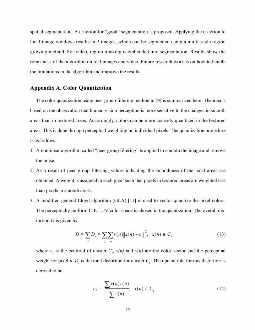
Appendix A. Color Quantization

The color quantization using peer group filtering method in [9] is summarized here. The idea is

based on the observation that human vision perception is more sensitive to the changes in smooth

areas than in textured areas. Accordingly, colors can be more coarsely quantized in the textured

areas. This is done through perceptual weighting on individual pixels. The quantization procedure

is as follows:

1. A nonlinear algorithm called “peer group filtering” is applied to smooth the image and remove

the noise.

2. As a result of peer group filtering, values indicating the smoothness of the local areas are

obtained. A weight is assigned to each pixel such that pixels in textured areas are weighted less

than pixels in smooth areas.

3. A modified general Lloyd algorithm (GLA) [11] is used to vector quantize the pixel colors.

The perceptually uniform CIE LUV color space is chosen in the quantization. The overall dis-

tortion D is given by

(13)

where ci is the centroid of cluster Ci, x(n) and v(n) are the color vector and the perceptual

weight for pixel n, Di is the total distortion for cluster Ci. The update rule for this distortion is

derived to be

(14)

D Dii∑ v n( ) x n( ) ci– 2

n∑

i∑= = x n( ) Ci∈,

ci

v n( )x n( )∑v n( )∑

----------------------------- x n( ) Ci∈,=

15

An initial estimate on the number of clusters is set to be slightly larger than the actual need.

The correctness of the estimation is not critical because clusters will be merged in Step 4.

4. After GLA, a large number of pixels having approximately the same color will have more than

one cluster because GLA is aimed to the minimize the global distortion. An agglomerative

clustering algorithm [10] is performed on the cluster centroids to further merge close clusters

such that the minimum distance between two centroids satisfies a preset threshold. This thresh-

old is the quantization parameter mentioned in the paper.

Acknowledgments

This work was supported in part by a grant from Samsung Electronics Co.

References

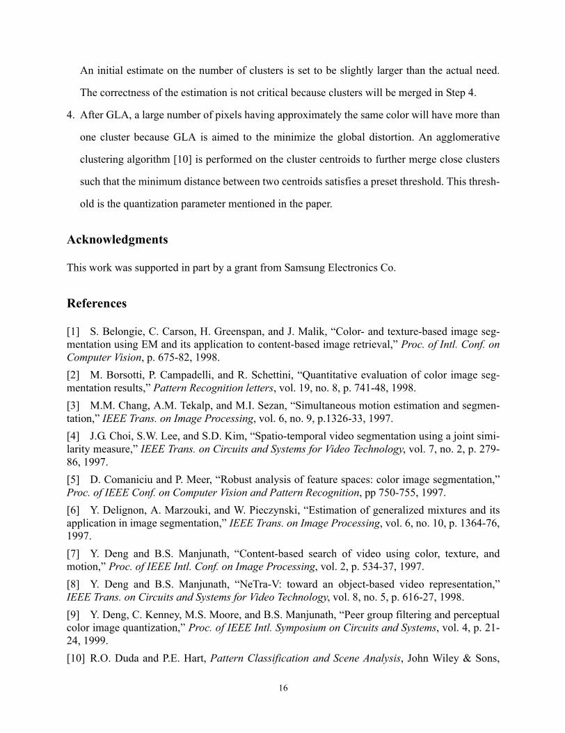
[1] S. Belongie, C. Carson, H. Greenspan, and J. Malik, “Color- and texture-based image seg-mentation using EM and its application to content-based image retrieval,” Proc. of Intl. Conf. onComputer Vision, p. 675-82, 1998. [2] M. Borsotti, P. Campadelli, and R. Schettini, “Quantitative evaluation of color image seg-mentation results,” Pattern Recognition letters, vol. 19, no. 8, p. 741-48, 1998. [3] M.M. Chang, A.M. Tekalp, and M.I. Sezan, “Simultaneous motion estimation and segmen-tation,” IEEE Trans. on Image Processing, vol. 6, no. 9, p.1326-33, 1997. [4] J.G. Choi, S.W. Lee, and S.D. Kim, “Spatio-temporal video segmentation using a joint simi-larity measure,” IEEE Trans. on Circuits and Systems for Video Technology, vol. 7, no. 2, p. 279-86, 1997.[5] D. Comaniciu and P. Meer, “Robust analysis of feature spaces: color image segmentation,”Proc. of IEEE Conf. on Computer Vision and Pattern Recognition, pp 750-755, 1997. [6] Y. Delignon, A. Marzouki, and W. Pieczynski, “Estimation of generalized mixtures and itsapplication in image segmentation,” IEEE Trans. on Image Processing, vol. 6, no. 10, p. 1364-76,1997.[7] Y. Deng and B.S. Manjunath, “Content-based search of video using color, texture, andmotion,” Proc. of IEEE Intl. Conf. on Image Processing, vol. 2, p. 534-37, 1997.[8] Y. Deng and B.S. Manjunath, “NeTra-V: toward an object-based video representation,”IEEE Trans. on Circuits and Systems for Video Technology, vol. 8, no. 5, p. 616-27, 1998.[9] Y. Deng, C. Kenney, M.S. Moore, and B.S. Manjunath, “Peer group filtering and perceptualcolor image quantization,” Proc. of IEEE Intl. Symposium on Circuits and Systems, vol. 4, p. 21-24, 1999.[10] R.O. Duda and P.E. Hart, Pattern Classification and Scene Analysis, John Wiley & Sons,

16

New York, 1970. [11] A. Gersho and R. M. Gray, Vector quantization and signal compression, Kluwer Academic,Norwell, MA, 1992.[12] G. Halevi and D. Weinshall, “Motion of disturbances: detection and tracking of multi-bodynon-rigid motion,” Proc. of IEEE Conf. on Computer Vision and Pattern Recognition, 897-902,1997.[13] D.A. Langan, J.W. Modestino, and J. Zhang, “Cluster validation for unsupervised stochasticmodel-based image segmentation,” IEEE Trans. on Image Processing, vol. 7, no. 2, p. 180-44,1997.[14] W.Y. Ma and B.S. Manjunath, “Edge flow: a framework of boundary detection and imagesegmentation,” Proc. of IEEE Conf. on Computer Vision and Pattern Recognition, pp 744-49,1997.[15] T. Meier and K.N. Ngan. “Automatic segmentation of moving objects for video object planegeneration,” IEEE Trans. on Circuits and Systems for Video Technology, vol. 8, no. 5, p. 525-38,1998. [16] F. Moscheni, S. Bhattacharjee, and M. Kunt, “Spatio-temporal segmentation based on regionmerging,” IEEE Trans. on Pattern Analysis and Machine Intelligence, vol. 20, no. 9, p. 897-915,1998.[17] D.K. Panjwani and G. Healey, “Markov random field models for unsupervised segmentationof textured color images,” IEEE Trans. on Pattern Analysis and Machine Intelligence, vol. 17, no.10, p. 939-54, 1995.[18] L. Shafarenko, M. Petrou, and J. Kittler, “Automatic watershed segmentation of randomlytextured color images,” IEEE Trans. on Image Processing, vol. 6, no. 11, p. 1530-44, 1997.[19] J. Shi and J. Malik, “Motion segmentation and tracking using normalized cuts,” Proc. ofIEEE 6th Intl. Conf. on Computer Vision, p.1154-60, 1998.[20] J. Shi and J. Malik, “Normalized cuts and image segmentation,” IEEE Trans. on PatternAnalysis and Machine Intelligence, vol. 22, no. 8, p. 888-905, 2000.[21] C. Stiller, “Object-based estimation of dense motion fields,” IEEE Trans. on Image Process-ing, vol. 6, no. 2, p. 234-50, 1997. [22] D. Wang, “Unsupervised video segmentation based on watersheds and temporal tracking,”IEEE Trans. on Circuits and Systems for Video Technology, vol. 8, no. 5, p. 539-46, 1998.[23] J. Wang and E. Adelson, “Representing moving images with layers,” IEEE Trans. on ImageProcessing, vol. 3, no. 5, p. 625-638, 1994.[24] J.-P. Wang, “Stochastic relaxation on partitions with connected components and its applica-tion to image segmentation,” IEEE Trans. on Pattern Analysis and Machine Intelligence, vol. 20,no.6, p. 619-36, 1998. [25] S.C. Zhu and A. Yuille, “Region competition: unifying snakes, region growing, and Bayes/MDL for multiband image segmentation,” IEEE Trans. on Pattern Analysis and Machine Intelli-gence, vol. 18, no. 9, p. 884-900.

17

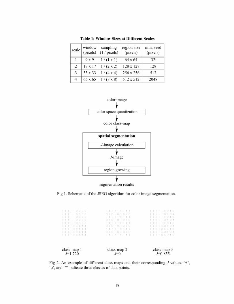
Table 1: Window Sizes at Different Scales

scale window(pixels)

sampling(1 / pixels)

region size(pixels)

min. seed(pixels)

1 9 x 9 1 / (1 x 1) 64 x 64 322 17 x 17 1 / (2 x 2) 128 x 128 1283 33 x 33 1 / (4 x 4) 256 x 256 5124 65 x 65 1 / (8 x 8) 512 x 512 2048

color space quantization

spatial segmentation

color image

color class-map

segmentation results

Fig 1. Schematic of the JSEG algorithm for color image segmentation.

J-image calculation

region growing

J-image

class-map 1J=1.720

class-map 2J=0

class-map 3J=0.855

Fig 2. An example of different class-maps and their corresponding J values. ‘+’,‘o’, and ‘*’ indicate three classes of data points.

18

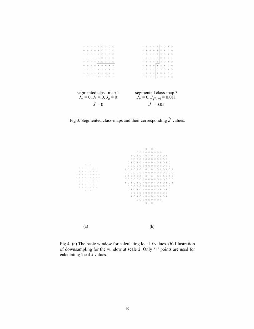
segmented class-map 1J+ = 0, J* = 0, Jo = 0

= 0J

segmented class-map 3J+ = 0, J{*, o} = 0.011

= 0.05J

Fig 3. Segmented class-maps and their corresponding values. J

Fig 4. (a) The basic window for calculating local J values. (b) Illustrationof downsampling for the window at scale 2. Only ‘+’ points are used forcalculating local J values.

(a) (b)

19

region growing

calculate local J values

original class-map

segmented regions

final results

scale < threshold?

..

initial scale

yesno

reduce scale

Fig 5. Flow-chart of the steps in spatial segmentation.

for each region

seed growing

seed determination

region merge

20

(a) (b) (c)

(d) (e) (f)

(g)

Fig 6. (a) A color image from the “flowergarden” video sequence (frame 0). (b)Result of color quantization with 13 col-ors. (c) J-image at scale 3. (d) J-image atscale 2. (e) Result after segmentation atscale 3. (f) Result after segmentation atscale 2. (g) Final result of segmentationafter merging.

size: 352 x 240

original (a): = 0.435scale 3 (e): = 0.103scale 2 (f): = 0.125final (g): = 0.088

J

JJ

J

21

seed tracking

calculate J

original class-maps

segmented objects

final results

scale < threshold?

...

initial scale

yesno

reduce scale by 1

Fig 7. Flow-chart of the steps in video spatio-temporal segmentation. Shaded blocksare new procedures introduced for video segmentation.

for each object

object merge

color quantization

P consecutive video frames

calculate J calculate J

frame 0 frame i frame P-1... ...

determineseed

determineseed

determineseed

seedgrowing

seedgrowing

seedgrowing

post-processing

22

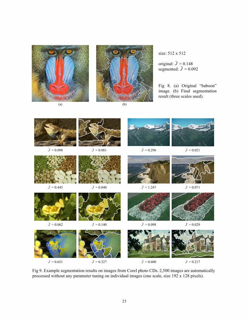
Fig 8. (a) Original “baboon”image. (b) Final segmentationresult (three scales used).

(a) (b)

size: 512 x 512

original: = 0.148segmented: = 0.092

JJ

Fig 9. Example segmentation results on images from Corel photo CDs. 2,500 images are automaticallyprocessed without any parameter tuning on individual images (one scale, size 192 x 128 pixels).

= 0.081J = 0.098J = 0.021J = 0.296J

= 0.040J = 0.445J = 0.071J = 1.247J

= 0.140J = 0.062J = 0.029J = 0.098J

= 0.327J = 0.651J = 0.217J = 0.600J

23

(a) manual (b) JSEG (1.99%) (c) manual (d) JSEG (2.09%)

Fig 10. Evaluation of segmentation results. Two images are manually segmented ((a) and (c)). Thecorresponding segmentation results using JSEG are shown in (b) and (d). The percentages of pixelslabeled differently by the JSEG segmentation are given in the parenthesis.

Fig 11. Segmentation of gray-scale images. The corresponding color image results are in Fig. 10.

Fig 12. Segmentation of illusionary contours. Background is dimmed to show the segmentation contours.

Fig 13. An example of Jt values calculated during the segmentation on “foreman” sequence: (a) Frame130. (b) Frame 131. (c) Jt values for the corresponding two frames shown as a gray scale image. Brightspots correspond to object motion.

(a) (b) (c)

24

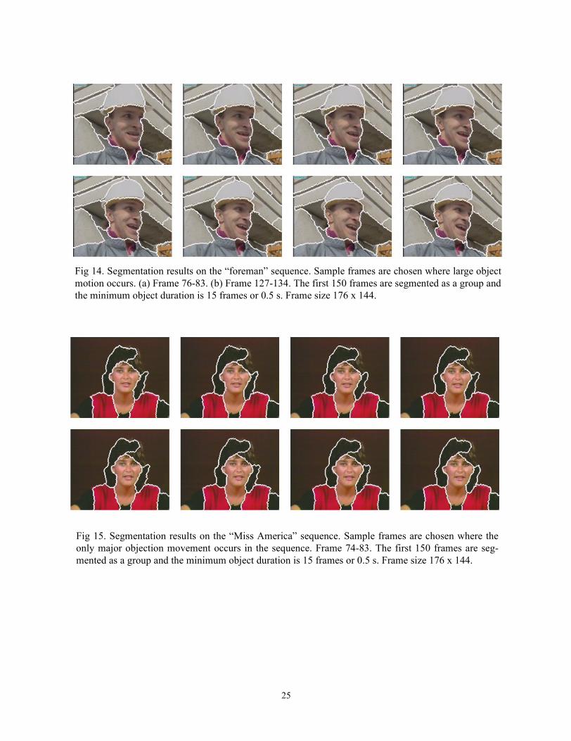
Fig 14. Segmentation results on the “foreman” sequence. Sample frames are chosen where large objectmotion occurs. (a) Frame 76-83. (b) Frame 127-134. The first 150 frames are segmented as a group andthe minimum object duration is 15 frames or 0.5 s. Frame size 176 x 144.

Fig 15. Segmentation results on the “Miss America” sequence. Sample frames are chosen where theonly major objection movement occurs in the sequence. Frame 74-83. The first 150 frames are seg-mented as a group and the minimum object duration is 15 frames or 0.5 s. Frame size 176 x 144.

25

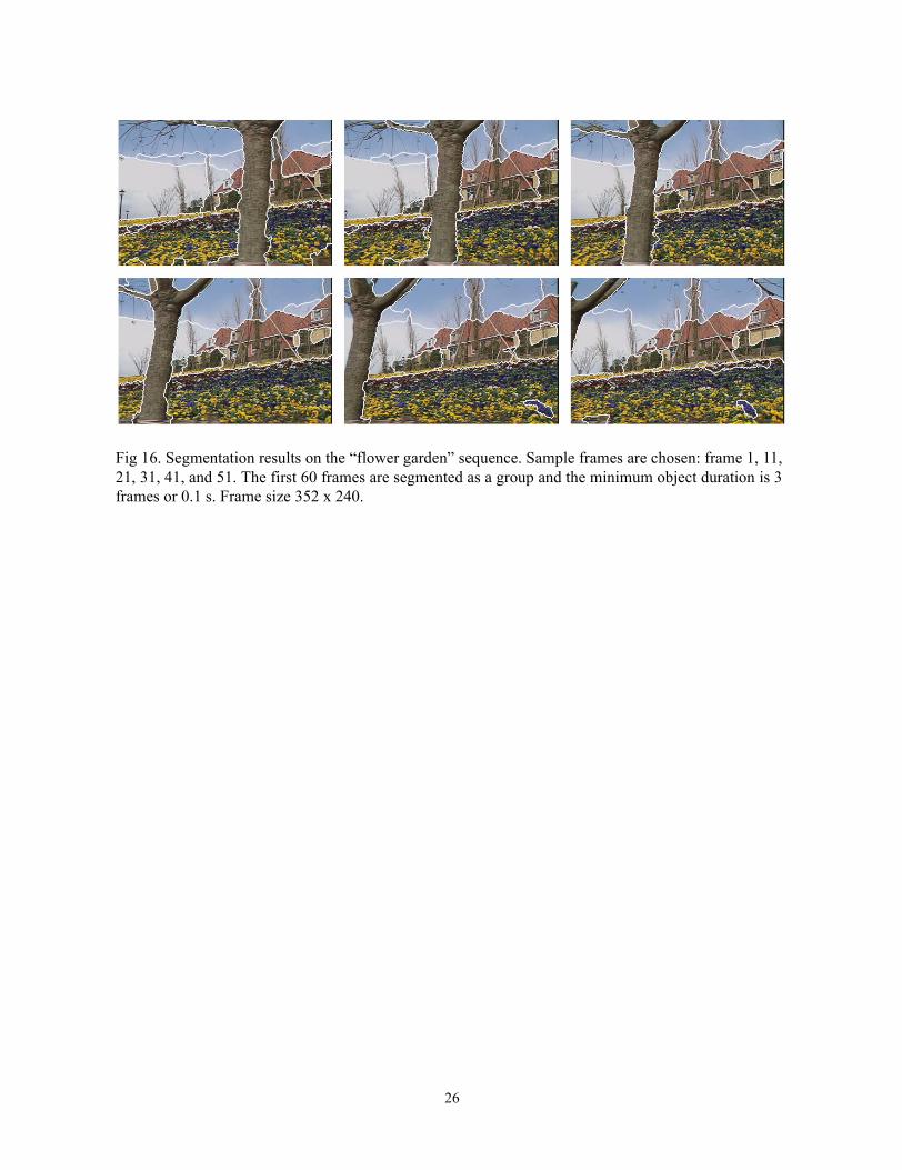
Fig 16. Segmentation results on the “flower garden” sequence. Sample frames are chosen: frame 1, 11,21, 31, 41, and 51. The first 60 frames are segmented as a group and the minimum object duration is 3frames or 0.1 s. Frame size 352 x 240.

26

27