Unsupervised segmentation and classification of cervical...

Pattern Recognition 45 (2012) 4151–4168

Contents lists available at SciVerse ScienceDirect

Pattern Recognition

0031-32

http://d

n Corr

E-m

saksoy@1 Pr

Univers

journal homepage: www.elsevier.com/locate/pr

Unsupervised segmentation and classification of cervical cell images

Aslı Genc-tav a,1, Selim Aksoy a,n, Sevgen Onder b

a Department of Computer Engineering, Bilkent University, Ankara 06800, Turkeyb Department of Pathology, Hacettepe University, Ankara 06100, Turkey

a r t i c l e i n f o

Article history:

Received 1 August 2011

Received in revised form

18 April 2012

Accepted 2 May 2012Available online 18 May 2012

Keywords:

Pap smear test

Cell grading

Automatic thresholding

Hierarchical segmentation

Multi-scale segmentation

Hierarchical clustering

Ranking

Optimal leaf ordering

03/$ - see front matter & 2012 Elsevier Ltd. A

x.doi.org/10.1016/j.patcog.2012.05.006

esponding author. Tel.: þ90 312 2903405; fa

ail addresses: [email protected] (A. Genc-t

cs.bilkent.edu.tr (S. Aksoy), sonder@hacettep

esent address: Department of Computer Engin

ity, Ankara 06531, Turkey.

a b s t r a c t

The Pap smear test is a manual screening procedure that is used to detect precancerous changes in

cervical cells based on color and shape properties of their nuclei and cytoplasms. Automating this

procedure is still an open problem due to the complexities of cell structures. In this paper, we propose

an unsupervised approach for the segmentation and classification of cervical cells. The segmentation

process involves automatic thresholding to separate the cell regions from the background, a multi-scale

hierarchical segmentation algorithm to partition these regions based on homogeneity and circularity,

and a binary classifier to finalize the separation of nuclei from cytoplasm within the cell regions.

Classification is posed as a grouping problem by ranking the cells based on their feature characteristics

modeling abnormality degrees. The proposed procedure constructs a tree using hierarchical clustering,

and then arranges the cells in a linear order by using an optimal leaf ordering algorithm that maximizes

the similarity of adjacent leaves without any requirement for training examples or parameter

adjustment. Performance evaluation using two data sets show the effectiveness of the proposed

approach in images having inconsistent staining, poor contrast, and overlapping cells.

& 2012 Elsevier Ltd. All rights reserved.

1. Introduction

Cervical cancer is the second most common type of canceramong women with more than 250,000 deaths every year [1].Fortunately, cervical cancer can be cured when early cancerouschanges or precursor lesions caused by the Human PapillomaVirus (HPV) are detected. However, the cure rate is closely relatedto the stage of the disease at diagnosis time, with a very highprobability of fatality if it is left untreated. Therefore, timelyidentification of the positive cases is crucial.

Since the discovery of a screening test, namely the Pap test,introduced by Dr. Georges Papanicolaou in the 1940s, a substantialdecrease in the rate of cervical cancer and the related mortality wasobserved. The Pap test has been the most effective cancer screeningtest ever, and still remains the crucial modality in detecting theprecursor lesions for cervical cancer. The test is based on obtainingcells from the uterine cervix, and smearing them onto glass slidesfor microscopic examination to detect HPV effects. The slides arestained using the Papanicolaou method where different componentsof the cells show different colors so that their examination becomeseasier (see Figs. 1 and 2 for examples).

ll rights reserved.

x: þ90 312 2664047.

av),

e.edu.tr (S. Onder).

eering, Middle East Technical

There are certain factors associated with the sensitivity of thePap test, and thus, the reliability of the diagnosis. The sensitivityof the test is hampered mostly by the quality of sampling(e.g., number of cells) and smearing (e.g., presence of obscuringelements such as blood, mucus, and inflammatory cells, or poorlyfixation of specimens). Both intra- and inter-observer variabilitiesduring the interpretation of the abnormal smears also contributeto the wide variation in false-negative results [2]. The promise ofearly diagnosis as well as the associated difficulties in the manualscreening process have made the development of automated orsemi-automated systems that analyze images acquired by using adigital camera connected to the microscope an importantresearch problem where more robust, consistent, and quantifiableexamination of the smears is expected to increase the reliabilityof the diagnosis [3,4].

Both automated and semi-automated screening proceduresinvolve two main tasks: segmentation and classification. Segmen-tation mainly focuses on separation of the cells from the back-ground as well as separation of the nuclei from the cytoplasmwithin the cell regions. Automatic thresholding, morphologicaloperations, and active contour models appear to be the mostpopular and common choices for the segmentation task in theliterature. For example, Bamford and Lovell [5] segmented thenucleus in a Pap smear image using an active contour model thatwas estimated by using dynamic programming to find theboundary with the minimum cost within a bounded space aroundthe darkest point in the image. Wu et al. [6] found the boundary

www.elsevier.com/locate/pr

www.elsevier.com/locate/pr

dx.doi.org/10.1016/j.patcog.2012.05.006



mailto:[email protected]






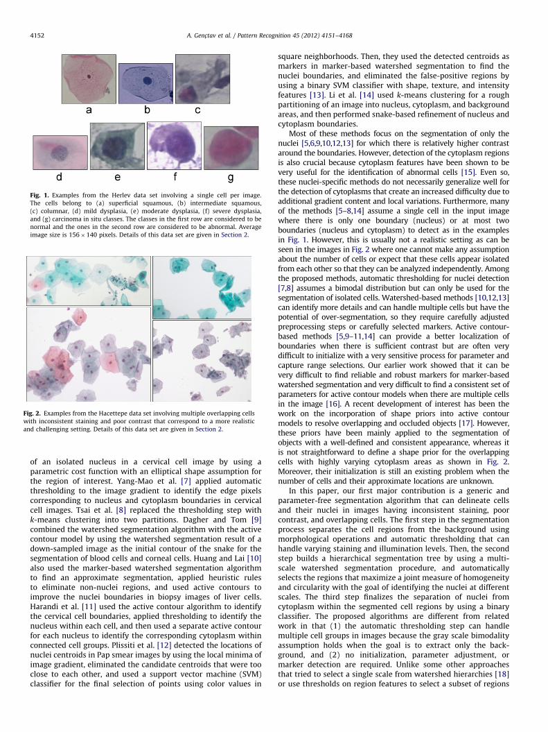
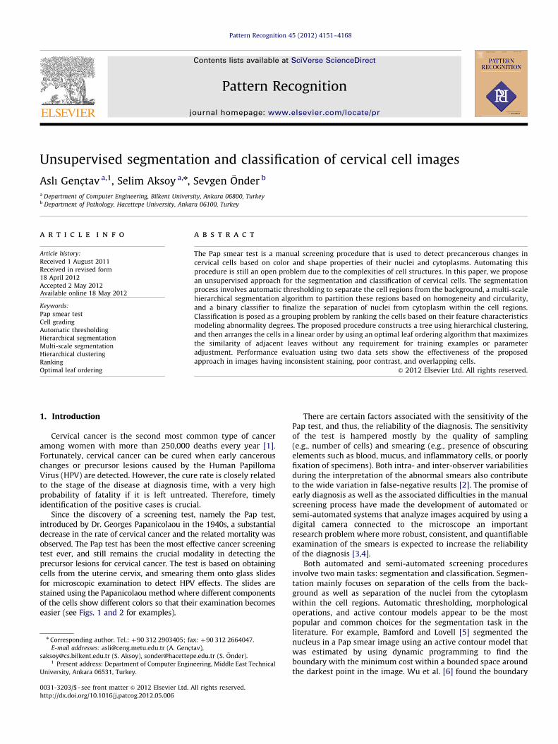
Fig. 1. Examples from the Herlev data set involving a single cell per image.

The cells belong to (a) superficial squamous, (b) intermediate squamous,

(c) columnar, (d) mild dysplasia, (e) moderate dysplasia, (f) severe dysplasia,

and (g) carcinoma in situ classes. The classes in the first row are considered to be

normal and the ones in the second row are considered to be abnormal. Average

image size is 156�140 pixels. Details of this data set are given in Section 2.

Fig. 2. Examples from the Hacettepe data set involving multiple overlapping cells

with inconsistent staining and poor contrast that correspond to a more realistic

and challenging setting. Details of this data set are given in Section 2.

A. Genc-tav et al. / Pattern Recognition 45 (2012) 4151–41684152

of an isolated nucleus in a cervical cell image by using aparametric cost function with an elliptical shape assumption forthe region of interest. Yang-Mao et al. [7] applied automaticthresholding to the image gradient to identify the edge pixelscorresponding to nucleus and cytoplasm boundaries in cervicalcell images. Tsai et al. [8] replaced the thresholding step withk-means clustering into two partitions. Dagher and Tom [9]combined the watershed segmentation algorithm with the activecontour model by using the watershed segmentation result of adown-sampled image as the initial contour of the snake for thesegmentation of blood cells and corneal cells. Huang and Lai [10]also used the marker-based watershed segmentation algorithmto find an approximate segmentation, applied heuristic rulesto eliminate non-nuclei regions, and used active contours toimprove the nuclei boundaries in biopsy images of liver cells.Harandi et al. [11] used the active contour algorithm to identifythe cervical cell boundaries, applied thresholding to identify thenucleus within each cell, and then used a separate active contourfor each nucleus to identify the corresponding cytoplasm withinconnected cell groups. Plissiti et al. [12] detected the locations ofnuclei centroids in Pap smear images by using the local minima ofimage gradient, eliminated the candidate centroids that were tooclose to each other, and used a support vector machine (SVM)classifier for the final selection of points using color values in

square neighborhoods. Then, they used the detected centroids asmarkers in marker-based watershed segmentation to find thenuclei boundaries, and eliminated the false-positive regions byusing a binary SVM classifier with shape, texture, and intensityfeatures [13]. Li et al. [14] used k-means clustering for a roughpartitioning of an image into nucleus, cytoplasm, and backgroundareas, and then performed snake-based refinement of nucleus andcytoplasm boundaries.

Most of these methods focus on the segmentation of only thenuclei [5,6,9,10,12,13] for which there is relatively higher contrastaround the boundaries. However, detection of the cytoplasm regionsis also crucial because cytoplasm features have been shown to bevery useful for the identification of abnormal cells [15]. Even so,these nuclei-specific methods do not necessarily generalize well forthe detection of cytoplasms that create an increased difficulty due toadditional gradient content and local variations. Furthermore, manyof the methods [5–8,14] assume a single cell in the input imagewhere there is only one boundary (nucleus) or at most twoboundaries (nucleus and cytoplasm) to detect as in the examplesin Fig. 1. However, this is usually not a realistic setting as can beseen in the images in Fig. 2 where one cannot make any assumptionabout the number of cells or expect that these cells appear isolatedfrom each other so that they can be analyzed independently. Amongthe proposed methods, automatic thresholding for nuclei detection[7,8] assumes a bimodal distribution but can only be used for thesegmentation of isolated cells. Watershed-based methods [10,12,13]can identify more details and can handle multiple cells but have thepotential of over-segmentation, so they require carefully adjustedpreprocessing steps or carefully selected markers. Active contour-based methods [5,9–11,14] can provide a better localization ofboundaries when there is sufficient contrast but are often verydifficult to initialize with a very sensitive process for parameter andcapture range selections. Our earlier work showed that it can bevery difficult to find reliable and robust markers for marker-basedwatershed segmentation and very difficult to find a consistent set ofparameters for active contour models when there are multiple cellsin the image [16]. A recent development of interest has been thework on the incorporation of shape priors into active contourmodels to resolve overlapping and occluded objects [17]. However,these priors have been mainly applied to the segmentation ofobjects with a well-defined and consistent appearance, whereas itis not straightforward to define a shape prior for the overlappingcells with highly varying cytoplasm areas as shown in Fig. 2.Moreover, their initialization is still an existing problem when thenumber of cells and their approximate locations are unknown.

In this paper, our first major contribution is a generic andparameter-free segmentation algorithm that can delineate cellsand their nuclei in images having inconsistent staining, poorcontrast, and overlapping cells. The first step in the segmentationprocess separates the cell regions from the background usingmorphological operations and automatic thresholding that canhandle varying staining and illumination levels. Then, the secondstep builds a hierarchical segmentation tree by using a multi-scale watershed segmentation procedure, and automaticallyselects the regions that maximize a joint measure of homogeneityand circularity with the goal of identifying the nuclei at differentscales. The third step finalizes the separation of nuclei fromcytoplasm within the segmented cell regions by using a binaryclassifier. The proposed algorithms are different from relatedwork in that (1) the automatic thresholding step can handlemultiple cell groups in images because the gray scale bimodalityassumption holds when the goal is to extract only the back-ground, and (2) no initialization, parameter adjustment, ormarker detection are required. Unlike some other approachesthat tried to select a single scale from watershed hierarchies [18]or use thresholds on region features to select a subset of regions

Classificationof cervical cells

Ranking ofcells

Featureextraction

Segmentation of cervical cells

Input image Backgroundextraction

Nucleus andcytoplasm

segmentation

Nucleus andcytoplasm

classification

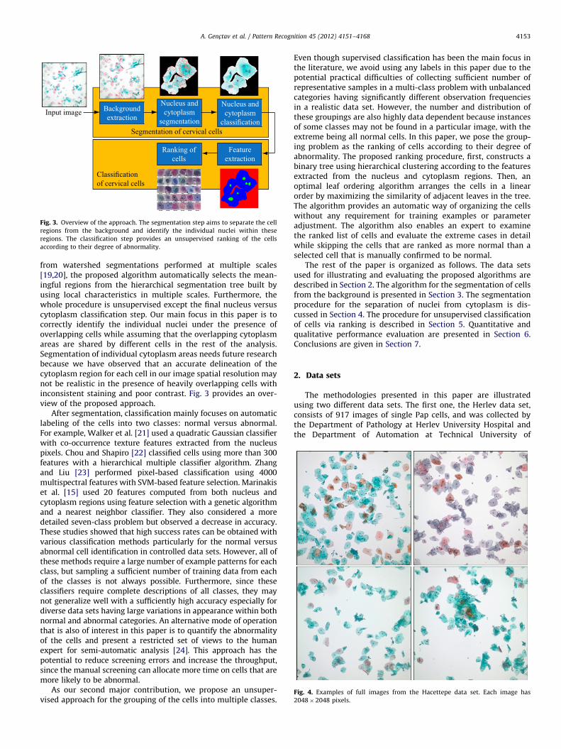
Fig. 3. Overview of the approach. The segmentation step aims to separate the cell

regions from the background and identify the individual nuclei within these

regions. The classification step provides an unsupervised ranking of the cells

according to their degree of abnormality.

Fig. 4. Examples of full images from the Hacettepe data set. Each image has

2048�2048 pixels.

A. Genc-tav et al. / Pattern Recognition 45 (2012) 4151–4168 4153

from watershed segmentations performed at multiple scales[19,20], the proposed algorithm automatically selects the mean-ingful regions from the hierarchical segmentation tree built byusing local characteristics in multiple scales. Furthermore, thewhole procedure is unsupervised except the final nucleus versuscytoplasm classification step. Our main focus in this paper is tocorrectly identify the individual nuclei under the presence ofoverlapping cells while assuming that the overlapping cytoplasmareas are shared by different cells in the rest of the analysis.Segmentation of individual cytoplasm areas needs future researchbecause we have observed that an accurate delineation of thecytoplasm region for each cell in our image spatial resolution maynot be realistic in the presence of heavily overlapping cells withinconsistent staining and poor contrast. Fig. 3 provides an over-view of the proposed approach.

After segmentation, classification mainly focuses on automaticlabeling of the cells into two classes: normal versus abnormal.For example, Walker et al. [21] used a quadratic Gaussian classifierwith co-occurrence texture features extracted from the nucleuspixels. Chou and Shapiro [22] classified cells using more than 300features with a hierarchical multiple classifier algorithm. Zhangand Liu [23] performed pixel-based classification using 4000multispectral features with SVM-based feature selection. Marinakiset al. [15] used 20 features computed from both nucleus andcytoplasm regions using feature selection with a genetic algorithmand a nearest neighbor classifier. They also considered a moredetailed seven-class problem but observed a decrease in accuracy.These studies showed that high success rates can be obtained withvarious classification methods particularly for the normal versusabnormal cell identification in controlled data sets. However, all ofthese methods require a large number of example patterns for eachclass, but sampling a sufficient number of training data from eachof the classes is not always possible. Furthermore, since theseclassifiers require complete descriptions of all classes, they maynot generalize well with a sufficiently high accuracy especially fordiverse data sets having large variations in appearance within bothnormal and abnormal categories. An alternative mode of operationthat is also of interest in this paper is to quantify the abnormalityof the cells and present a restricted set of views to the humanexpert for semi-automatic analysis [24]. This approach has thepotential to reduce screening errors and increase the throughput,since the manual screening can allocate more time on cells that aremore likely to be abnormal.

As our second major contribution, we propose an unsuper-vised approach for the grouping of the cells into multiple classes.

Even though supervised classification has been the main focus inthe literature, we avoid using any labels in this paper due to thepotential practical difficulties of collecting sufficient number ofrepresentative samples in a multi-class problem with unbalancedcategories having significantly different observation frequenciesin a realistic data set. However, the number and distribution ofthese groupings are also highly data dependent because instancesof some classes may not be found in a particular image, with theextreme being all normal cells. In this paper, we pose the group-ing problem as the ranking of cells according to their degree ofabnormality. The proposed ranking procedure, first, constructs abinary tree using hierarchical clustering according to the featuresextracted from the nucleus and cytoplasm regions. Then, anoptimal leaf ordering algorithm arranges the cells in a linearorder by maximizing the similarity of adjacent leaves in the tree.The algorithm provides an automatic way of organizing the cellswithout any requirement for training examples or parameteradjustment. The algorithm also enables an expert to examinethe ranked list of cells and evaluate the extreme cases in detailwhile skipping the cells that are ranked as more normal than aselected cell that is manually confirmed to be normal.

The rest of the paper is organized as follows. The data setsused for illustrating and evaluating the proposed algorithms aredescribed in Section 2. The algorithm for the segmentation of cellsfrom the background is presented in Section 3. The segmentationprocedure for the separation of nuclei from cytoplasm is dis-cussed in Section 4. The procedure for unsupervised classificationof cells via ranking is described in Section 5. Quantitative andqualitative performance evaluation are presented in Section 6.Conclusions are given in Section 7.

2. Data sets

The methodologies presented in this paper are illustratedusing two different data sets. The first one, the Herlev data set,consists of 917 images of single Pap cells, and was collected bythe Department of Pathology at Herlev University Hospital andthe Department of Automation at Technical University of


Denmark [25]. The images were acquired at a magnification of0:201 mm=pixel. Average image size is 156�140 pixels. Cyto-technicians and doctors manually classified each cell into one ofthe seven classes, namely superficial squamous, intermediatesquamous, columnar, mild dysplasia, moderate dysplasia, severedysplasia, and carcinoma in situ. The first three classes corre-spond to normal cells and the last four classes correspond toabnormal cells with examples in Fig. 1. Each cell also has anassociated ground truth of nucleus and cytoplasm regions.

The second data set, referred to as the Hacettepe data set, wascollected by the Department of Pathology at Hacettepe UniversityHospital using the ThinPrep liquid-based cytology preparationtechnique. It consists of 82 Pap test images belonging to 18different patients. Each image has 2048�2048 pixels, and wasacquired at 200X magnification. These images are more realisticwith the challenges of overlapping cells, poor contrast, andinconsistent staining with examples shown in Fig. 4. We manuallydelineated the nuclei in a subset of this data set for performanceevaluation. Both data sets are used for quantitative and qualita-tive evaluation in this paper.

3. Background extraction

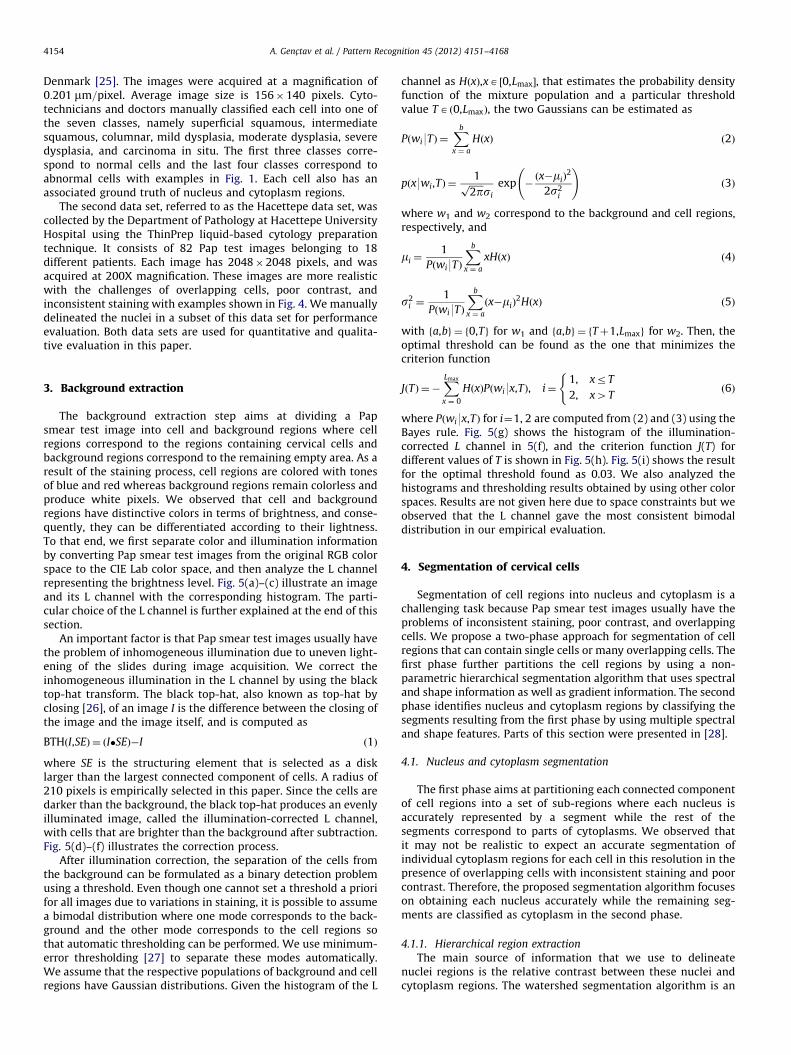
The background extraction step aims at dividing a Papsmear test image into cell and background regions where cellregions correspond to the regions containing cervical cells andbackground regions correspond to the remaining empty area. As aresult of the staining process, cell regions are colored with tonesof blue and red whereas background regions remain colorless andproduce white pixels. We observed that cell and backgroundregions have distinctive colors in terms of brightness, and conse-quently, they can be differentiated according to their lightness.To that end, we first separate color and illumination informationby converting Pap smear test images from the original RGB colorspace to the CIE Lab color space, and then analyze the L channelrepresenting the brightness level. Fig. 5(a)–(c) illustrate an imageand its L channel with the corresponding histogram. The parti-cular choice of the L channel is further explained at the end of thissection.

An important factor is that Pap smear test images usually havethe problem of inhomogeneous illumination due to uneven light-ening of the slides during image acquisition. We correct theinhomogeneous illumination in the L channel by using the blacktop-hat transform. The black top-hat, also known as top-hat byclosing [26], of an image I is the difference between the closing ofthe image and the image itself, and is computed as

BTHðI,SEÞ ¼ ðI�SEÞ�I ð1Þ

where SE is the structuring element that is selected as a disklarger than the largest connected component of cells. A radius of210 pixels is empirically selected in this paper. Since the cells aredarker than the background, the black top-hat produces an evenlyilluminated image, called the illumination-corrected L channel,with cells that are brighter than the background after subtraction.Fig. 5(d)–(f) illustrates the correction process.

After illumination correction, the separation of the cells fromthe background can be formulated as a binary detection problemusing a threshold. Even though one cannot set a threshold a priorifor all images due to variations in staining, it is possible to assumea bimodal distribution where one mode corresponds to the back-ground and the other mode corresponds to the cell regions sothat automatic thresholding can be performed. We use minimum-error thresholding [27] to separate these modes automatically.We assume that the respective populations of background and cellregions have Gaussian distributions. Given the histogram of the L

channel as HðxÞ,xA ½0,Lmax�, that estimates the probability densityfunction of the mixture population and a particular thresholdvalue TAð0,LmaxÞ, the two Gaussians can be estimated as

Pðwi9TÞ ¼Xb

x ¼ a

HðxÞ ð2Þ

pðx9wi,TÞ ¼1ffiffiffiffiffiffi

2pp

si

exp �ðx�miÞ

2

2s2i

!ð3Þ

where w1 and w2 correspond to the background and cell regions,respectively, and

mi ¼1

Pðwi9TÞ

Xb

x ¼ a

xHðxÞ ð4Þ

s2i ¼

1

Pðwi9TÞ

Xb

x ¼ a

ðx�miÞ2HðxÞ ð5Þ

with fa,bg ¼ f0,Tg for w1 and fa,bg ¼ fTþ1,Lmaxg for w2. Then, theoptimal threshold can be found as the one that minimizes thecriterion function

JðTÞ ¼ �XLmax

x ¼ 0

HðxÞPðwi9x,TÞ, i¼1, xrT

2, x4T

(ð6Þ

where Pðwi9x,TÞ for i¼1, 2 are computed from (2) and (3) using theBayes rule. Fig. 5(g) shows the histogram of the illumination-corrected L channel in 5(f), and the criterion function J(T) fordifferent values of T is shown in Fig. 5(h). Fig. 5(i) shows the resultfor the optimal threshold found as 0.03. We also analyzed thehistograms and thresholding results obtained by using other colorspaces. Results are not given here due to space constraints but weobserved that the L channel gave the most consistent bimodaldistribution in our empirical evaluation.

4. Segmentation of cervical cells

Segmentation of cell regions into nucleus and cytoplasm is achallenging task because Pap smear test images usually have theproblems of inconsistent staining, poor contrast, and overlappingcells. We propose a two-phase approach for segmentation of cellregions that can contain single cells or many overlapping cells. Thefirst phase further partitions the cell regions by using a non-parametric hierarchical segmentation algorithm that uses spectraland shape information as well as gradient information. The secondphase identifies nucleus and cytoplasm regions by classifying thesegments resulting from the first phase by using multiple spectraland shape features. Parts of this section were presented in [28].

4.1. Nucleus and cytoplasm segmentation

The first phase aims at partitioning each connected componentof cell regions into a set of sub-regions where each nucleus isaccurately represented by a segment while the rest of thesegments correspond to parts of cytoplasms. We observed thatit may not be realistic to expect an accurate segmentation ofindividual cytoplasm regions for each cell in this resolution in thepresence of overlapping cells with inconsistent staining and poorcontrast. Therefore, the proposed segmentation algorithm focuseson obtaining each nucleus accurately while the remaining seg-ments are classified as cytoplasm in the second phase.

4.1.1. Hierarchical region extraction

The main source of information that we use to delineatenuclei regions is the relative contrast between these nuclei andcytoplasm regions. The watershed segmentation algorithm is an

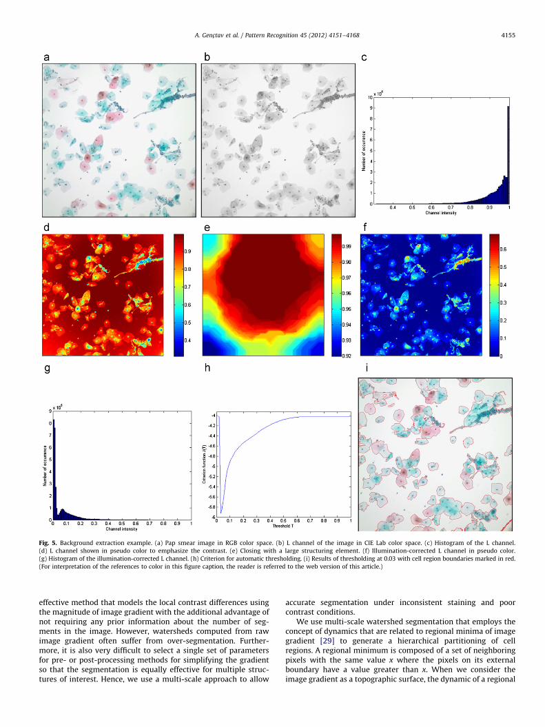
Fig. 5. Background extraction example. (a) Pap smear image in RGB color space. (b) L channel of the image in CIE Lab color space. (c) Histogram of the L channel.

(d) L channel shown in pseudo color to emphasize the contrast. (e) Closing with a large structuring element. (f) Illumination-corrected L channel in pseudo color.

(g) Histogram of the illumination-corrected L channel. (h) Criterion for automatic thresholding. (i) Results of thresholding at 0.03 with cell region boundaries marked in red.

(For interpretation of the references to color in this figure caption, the reader is referred to the web version of this article.)


effective method that models the local contrast differences usingthe magnitude of image gradient with the additional advantage ofnot requiring any prior information about the number of seg-ments in the image. However, watersheds computed from rawimage gradient often suffer from over-segmentation. Further-more, it is also very difficult to select a single set of parametersfor pre- or post-processing methods for simplifying the gradientso that the segmentation is equally effective for multiple struc-tures of interest. Hence, we use a multi-scale approach to allow

accurate segmentation under inconsistent staining and poorcontrast conditions.

We use multi-scale watershed segmentation that employs theconcept of dynamics that are related to regional minima of imagegradient [29] to generate a hierarchical partitioning of cellregions. A regional minimum is composed of a set of neighboringpixels with the same value x where the pixels on its externalboundary have a value greater than x. When we consider theimage gradient as a topographic surface, the dynamic of a regional


minimum can be defined as the minimum height that a point inthe minimum has to climb to reach a lower regional minimum.

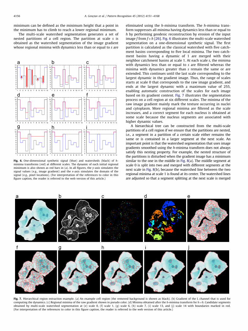
The multi-scale watershed segmentation generates a set ofnested partitions of a cell region. The partition at scale s isobtained as the watershed segmentation of the image gradientwhose regional minima with dynamics less than or equal to s are

Fig. 6. One-dimensional synthetic signal (blue) and watersheds (black) of h-

minima transforms (red) at different scales. The dynamic of each initial regional

minimum is also shown as red bars in (a). In all figures, the y-axis simulates the

signal values (e.g., image gradient) and the x-axis simulates the domain of the

signal (e.g., pixel locations). (For interpretation of the references to color in this

figure caption, the reader is referred to the web version of this article.)

Fig. 7. Hierarchical region extraction example. (a) An example cell region (the remov

computing the dynamics. (c) Regional minima of the raw gradient shown in pseudo colo

obtained by multi-scale watershed segmentation at (e) scale 0, (f) scale 1, (g) scal

(For interpretation of the references to color in this figure caption, the reader is referr

eliminated using the h-minima transform. The h-minima trans-form suppresses all minima having dynamics less than or equal toh by performing geodesic reconstruction by erosion of the inputimage f from fþh [26]. Fig. 6 illustrates the multi-scale watershedsegmentation on a one-dimensional synthetic signal. The firstpartition is calculated as the classical watershed with five catch-ment basins corresponding to five local minima. The two catch-ment basins having a dynamic of 1 are merged with theirneighbor catchment basins at scale 1. At each scale s, the minimawith dynamics less than or equal to s are filtered whereas theminima with dynamics greater than s remain the same or areextended. This continues until the last scale corresponding to thelargest dynamic in the gradient image. Thus, the range of scalesstarts at scale 0 that corresponds to the raw image gradient, andends at the largest dynamic with a maximum value of 255,enabling automatic construction of the scales for each imagebased on its gradient content. Fig. 7 illustrates the segmentationprocess on a cell region at six different scales. The minima of theraw image gradient mainly mark the texture occurring in nucleiand cytoplasm. More regional minima are filtered as the scaleincreases, and a correct segment for each nucleus is obtained atsome scale because the nucleus segments are associated withhigher dynamic values.

A hierarchical tree can be constructed from the multi-scalepartitions of a cell region if we ensure that the partitions are nested,i.e., a segment in a partition of a certain scale either remains thesame or is contained in a larger segment at the next scale. Animportant point is that the watershed segmentation that uses imagegradients smoothed using the h-minima transform does not alwayssatisfy this nesting property. For example, the nested structure ofthe partitions is disturbed when the gradient image has a minimumsimilar to the one in the middle in Fig. 8(a). The middle segment atscale 0 is split into two and merged with different segments at thenext scale in Fig. 8(b), because the watershed line between the tworegional minima at scale 1 is found at its center. The watershed linesare adjusted so that a segment splitting at the next scale is merged

ed background is shown as black). (b) Gradient of the L channel that is used for

r. (d) Minima obtained after the h-minima transform for h¼6. Candidate segments

e 6, (h) scale 7, (i) scale 13, and (j) scale 14 with boundaries marked in red.

ed to the web version of this article.)

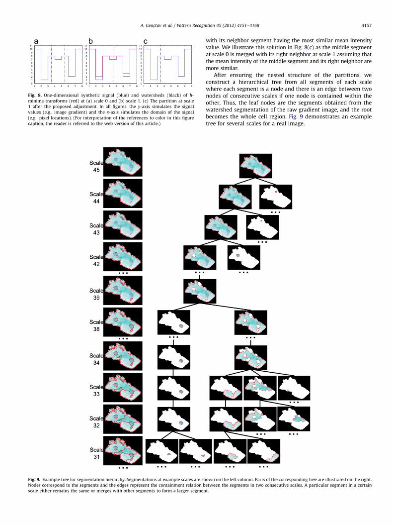
Fig. 8. One-dimensional synthetic signal (blue) and watersheds (black) of h-

minima transforms (red) at (a) scale 0 and (b) scale 1. (c) The partition at scale

1 after the proposed adjustment. In all figures, the y-axis simulates the signal

values (e.g., image gradient) and the x-axis simulates the domain of the signal

(e.g., pixel locations). (For interpretation of the references to color in this figure

caption, the reader is referred to the web version of this article.)

Fig. 9. Example tree for segmentation hierarchy. Segmentations at example scales are sh

Nodes correspond to the segments and the edges represent the containment relation b

scale either remains the same or merges with other segments to form a larger segmen


with its neighbor segment having the most similar mean intensityvalue. We illustrate this solution in Fig. 8(c) as the middle segmentat scale 0 is merged with its right neighbor at scale 1 assuming thatthe mean intensity of the middle segment and its right neighbor aremore similar.

After ensuring the nested structure of the partitions, weconstruct a hierarchical tree from all segments of each scalewhere each segment is a node and there is an edge between twonodes of consecutive scales if one node is contained within theother. Thus, the leaf nodes are the segments obtained from thewatershed segmentation of the raw gradient image, and the rootbecomes the whole cell region. Fig. 9 demonstrates an exampletree for several scales for a real image.

own on the left column. Parts of the corresponding tree are illustrated on the right.

etween the segments in two consecutive scales. A particular segment in a certain

t.

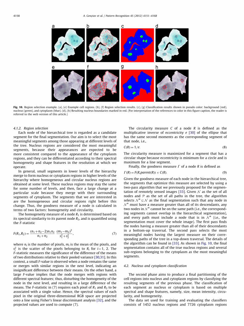
Fig. 10. Region selection example. (a), (e) Example cell regions. (b), (f) Region selection results. (c), (g) Classification results shown in pseudo color: background (red),

nucleus (green), and cytoplasm (blue). (d), (h) Resulting nucleus boundaries marked in red. (For interpretation of the references to color in this figure caption, the reader is

referred to the web version of this article.)


4.1.2. Region selection

Each node of the hierarchical tree is regarded as a candidatesegment for the final segmentation. Our aim is to select the mostmeaningful segments among those appearing at different levels ofthe tree. Nucleus regions are considered the most meaningfulsegments, because their appearances are expected to bemore consistent compared to the appearance of the cytoplasmregions, and they can be differentiated according to their spectralhomogeneity and shape features in the resolution at which weoperate.

In general, small segments in lower levels of the hierarchymerge to form nucleus or cytoplasm regions in higher levels of thehierarchy where homogeneous and circular nucleus regions areobtained at some level. These nucleus regions may stay the samefor some number of levels, and then, face a large change at aparticular scale because they merge with their surroundingsegments of cytoplasm. The segments that we are interested inare the homogeneous and circular regions right before thischange. Thus, the goodness measure of a node is calculated interms of two factors: homogeneity and circularity.

The homogeneity measure of a node R1 is determined based onits spectral similarity to its parent node R2, and is quantified usingthe F-statistic

FðR1,R2Þ ¼ðn1þn2�2Þn1n2

n1þn2

ðm1�m2Þ2

s21þs2

2

, ð7Þ

where ni is the number of pixels, mi is the mean of the pixels, ands2

i is the scatter of the pixels belonging to Ri for i¼1, 2. TheF-statistic measures the significance of the difference of the meansof two distributions relative to their pooled variance [30,31]. In thiscontext, a small F-value is observed when a node remains the sameor merges with similar regions in the next level, indicating aninsignificant difference between their means. On the other hand, alarge F-value implies that the node merges with regions withdifferent spectral features; thus, disturbing the homogeneity of thenode in the next level, and resulting in a large difference of themeans. The F-statistic in (7) requires each pixel of R1 and R2 to beassociated with a single value. Hence, the spectral values of eachpixel in the original three-dimensional RGB space are projectedonto a line using Fisher’s linear discriminant analysis [32], and theprojected values are used to compute (7).

The circularity measure C of a node R is defined as themultiplicative inverse of eccentricity e [30] of the ellipse thathas the same second moments as the corresponding segment ofthat node, i.e.,

CðRÞ ¼ 1=e: ð8Þ

The circularity measure is maximized for a segment that has acircular shape because eccentricity is minimum for a circle and ismaximum for a line segment.

Finally, the goodness measure G of a node R is defined as

GðRÞ ¼ FðR,parentðRÞÞ � CðRÞ: ð9Þ

Given the goodness measure of each node in the hierarchical tree,the segments that optimize this measure are selected by using atwo-pass algorithm that we previously proposed for the segmen-tation of remotely sensed images [33]. Given N as the set of allnodes and P as the set of all paths in the tree, the algorithmselects N nDN as the final segmentation such that any node inN n must have a measure greater than all of its descendants, anytwo nodes in N n cannot be on the same path (i.e., the correspond-ing segments cannot overlap in the hierarchical segmentation),and every path must include a node that is in N n (i.e., thesegmentation must cover the whole image). The first pass findsthe nodes having a measure greater than all of their descendantsin a bottom-up traversal. The second pass selects the mostmeaningful nodes having the largest measure on their corre-sponding paths of the tree in a top-down traversal. The details ofthe algorithm can be found in [33]. As shown in Fig. 10, the finalsegmentation contains all of the true nucleus regions and severalsub-regions belonging to the cytoplasm as the most meaningfulsegments.

4.2. Nucleus and cytoplasm classification

The second phase aims to produce a final partitioning of thecell regions into nucleus and cytoplasm regions by classifying theresulting segments of the previous phase. The classification ofeach segment as nucleus or cytoplasm is based on multiplespectral and shape features, namely, size, mean intensity, circu-larity, and homogeneity.

The data set used for training and evaluating the classifiersconsists of 1452 nucleus regions and 7726 cytoplasm regions

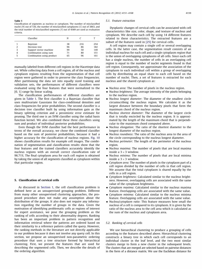
Table 1Classification of segments as nucleus or cytoplasm. The number of misclassified

nuclei (N) out of 726, the number of misclassified cytoplasms (C) out of 3863, and

the total number of misclassified segments (T) out of 4589 are used as evaluation

criteria.

Classifier N C T

1 Bayesian 38 216 254

2 Decision tree 96 86 182

3 Support vector machine 99 50 149

4 Combination using sum 71 80 151

5 Combination using product 65 96 161


manually labeled from different cell regions in the Hacettepe dataset. While collecting data from a cell region, all of the nucleus andcytoplasm regions resulting from the segmentation of that cellregion were gathered in order to preserve the class frequencies.After partitioning the data set into equally sized training andvalidation sets, the performances of different classifiers wereevaluated using the four features that were normalized to the[0, 1] range by linear scaling.

The classification performances of different classifiers aregiven in Table 1. The first classifier is a Bayesian classifier thatuses multivariate Gaussians for class-conditional densities andclass frequencies for prior probabilities. The second classifier is adecision tree classifier built by using information gain as thebinary splitting criterion and a pessimistic error estimate forpruning. The third one is an SVM classifier using the radial basisfunction kernel. We also combined these three classifiers usingsum and product of individual posterior probabilities.

Even though the SVM classifier had the best performance interms of the overall accuracy, we chose the combined classifierbased on the sum of posterior probabilities, because it had ahigher accuracy for the classification of nucleus regions. Fig. 10shows classification results for example cell images. The combi-nation of segmentation and classification results show that thefour features and the trained classifiers accurately identify thenucleus regions with an overall correct classification rate of96.71%. The final cytoplasm area for each cell region is obtainedby taking the union of all segments classified as cytoplasm withinthat particular region.

5. Classification of cervical cells

As discussed in Section 1, the cell classification problem isdefined here as an unsupervised grouping problem. Differentfrom many other unsupervised clustering approaches, the pro-posed procedure does not make any assumption about thedistribution of the groups. It also does not require any informa-tion regarding the number of groups in the data. Given themotivation of identifying problematic cells as regions of interestfor expert assistance, we pose the grouping problem as theranking of cells according to their abnormality degrees. Rankinghas been an important problem in pattern recognition andinformation retrieval where the patterns are ordered based ontheir similarity to a reference pattern called the query. However,the ranking methods in the literature are not directly applicableto our problem because it does not involve any query cell. In thissection, we propose an unsupervised non-parametric orderingprocedure that uses a tree structure formed by hierarchicalclustering. First, we present the features that are used fordescribing the segmented cells. Then, we describe the details ofthe ordering algorithm.

5.1. Feature extraction

Dysplastic changes of cervical cells can be associated with cellcharacteristics like size, color, shape, and texture of nucleus andcytoplasm. We describe each cell by using 14 different featuresrelated to these characteristics. The extracted features are asubset of the features used in [25] for cervical cells.

A cell region may contain a single cell or several overlappingcells. In the latter case, the segmentation result consists of anindividual nucleus for each cell and a single cytoplasm region thatis the union of overlapping cytoplasms of all cells. Since each cellhas a single nucleus, the number of cells in an overlapping cellregion is equal to the number of nuclei segments found in thatcell region. Consequently, we approximate the association of thecytoplasm to each individual cell within a group of overlappingcells by distributing an equal share to each cell based on thenumber of nuclei. Then, a set of features is extracted for eachnucleus and the shared cytoplasm as:

�
Nucleus area: The number of pixels in the nucleus region. � Nucleus brightness: The average intensity of the pixels belonging
to the nucleus region.
� Nucleus longest diameter: The diameter of the smallest circle
circumscribing the nucleus region. We calculate it as thelargest distance between the boundary pixels that form themaximum chord of the nucleus region.
� Nucleus shortest diameter: The diameter of the largest circle
that is totally encircled by the nucleus region. It is approxi-mated by the length of the maximum chord that is perpendi-cular to the maximum chord computed above.
� Nucleus elongation: The ratio of the shortest diameter to the
longest diameter of the nucleus region.
� Nucleus roundness: The ratio of the nucleus area to the area of
the circle corresponding to the nucleus longest diameter.
� Nucleus perimeter: The length of the perimeter of the nucleus
region.
� Nucleus maxima: The number of pixels that are local maxima
inside a 3�3 window.
� Nucleus minima: The number of pixels that are local minima
inside a 3�3 window.
� Cytoplasm area: The number of pixels in the cytoplasm part of a
cell region divided by the number of cells in that cell region.We assume that the total cytoplasm is shared equally by thecells in a cell region.
� Cytoplasm brightness: Calculated similar to the nucleus bright-
ness. However, overlapping cells are associated with the samevalue of the cytoplasm brightness.
� Cytoplasm maxima: Calculated similar to the nucleus maxima
feature. Overlapping cells are associated with the same value.
� Cytoplasm minima: Calculated similar to the nucleus minima
feature. Overlapping cells are associated with the same value.
� Nucleus/cytoplasm ratio: This feature measures how small the
nucleus of a cell is compared to its cytoplasm. It is given by theratio of the nucleus area to the cell area which is calculated asthe sum of the nucleus and cytoplasm area.

5.2. Ranking of cervical cells

We use hierarchical clustering to produce a grouping of cellsaccording to the features described above. Hierarchical clusteringconstructs a binary tree in which each cell corresponds to anindividual cluster in the leaf level, and the two most similarclusters merge to form a new cluster in the subsequent levels.The clusters that are merged are selected based on pairwise distancesin the form of a distance matrix. We use the Euclidean distance for


computing the pairwise feature distances and the average linkagecriterion to compute the distance between two clusters [32].

Hierarchical clustering and the resulting tree structure areintuitive ways of organizing the cells because the cells that areadjacent in the tree are assumed to be related with respect totheir feature characteristics. These relations can be converted to alinear ordering of the cells corresponding to the ordering of theleaf nodes. Let T be a binary tree with n leaf nodes denoted asz1, . . . ,zn, and n�1 non-leaf nodes denoted as y1, . . . ,yn�1. A linearordering that is consistent with T is defined to be an ordering ofthe leaves of T that is generated by flipping the non-leaf nodes ofT , i.e., swapping the left and right subtrees rooted at yi for anyyiAT [34]. A flipping operation at a particular node changes theorder of the subtrees of that node, and produces a differentordering of the leaves. Fig. 11 illustrates the flipping of subtreesat a node where the ordering of the leaves is changed while thesame tree structure is preserved. The possibility of applying aflipping operation at each of the n�1 non-leaf nodes of T resultsin a total of 2n�1 possible linear orderings of the leaves of T .

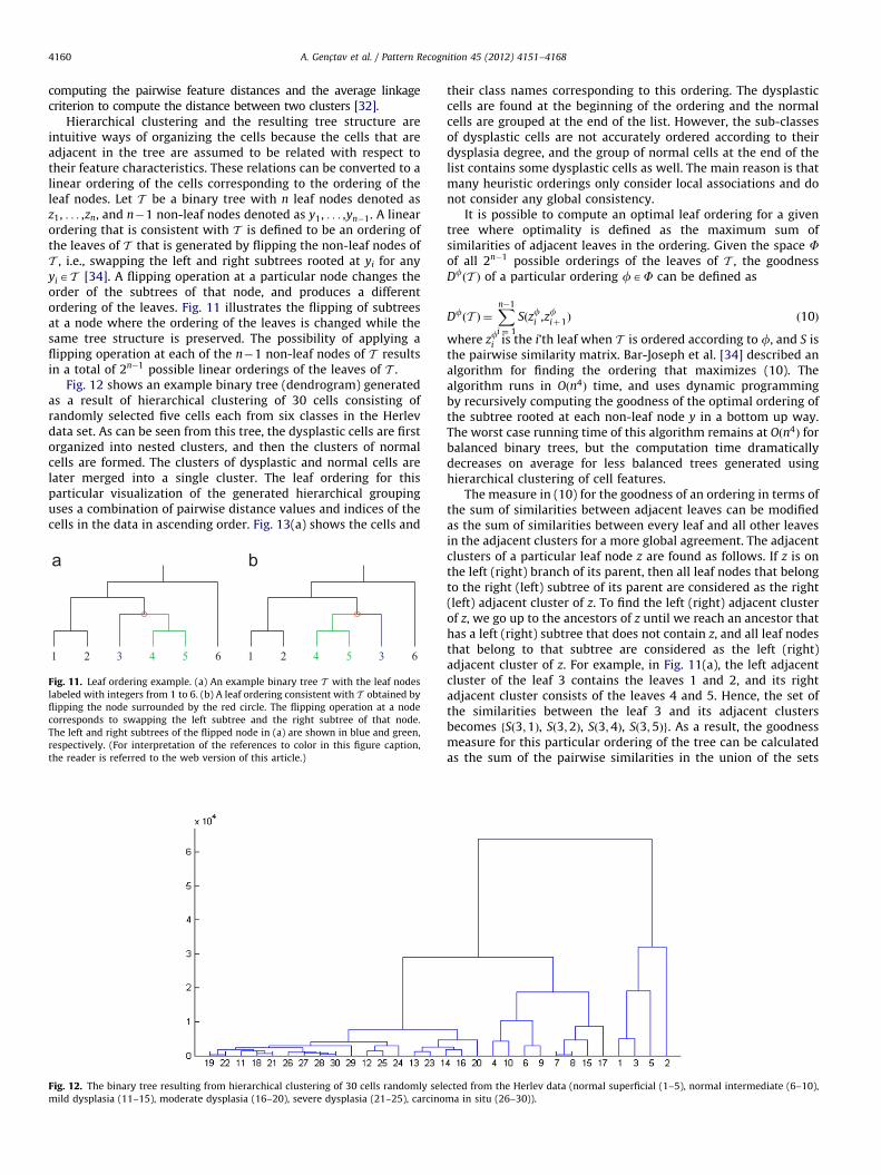
Fig. 12 shows an example binary tree (dendrogram) generatedas a result of hierarchical clustering of 30 cells consisting ofrandomly selected five cells each from six classes in the Herlevdata set. As can be seen from this tree, the dysplastic cells are firstorganized into nested clusters, and then the clusters of normalcells are formed. The clusters of dysplastic and normal cells arelater merged into a single cluster. The leaf ordering for thisparticular visualization of the generated hierarchical groupinguses a combination of pairwise distance values and indices of thecells in the data in ascending order. Fig. 13(a) shows the cells and

1 2 63 4 5 1 2 64 5 3

Fig. 11. Leaf ordering example. (a) An example binary tree T with the leaf nodes

labeled with integers from 1 to 6. (b) A leaf ordering consistent with T obtained by

flipping the node surrounded by the red circle. The flipping operation at a node

corresponds to swapping the left subtree and the right subtree of that node.

The left and right subtrees of the flipped node in (a) are shown in blue and green,

respectively. (For interpretation of the references to color in this figure caption,

the reader is referred to the web version of this article.)

Fig. 12. The binary tree resulting from hierarchical clustering of 30 cells randomly sele

mild dysplasia (11–15), moderate dysplasia (16–20), severe dysplasia (21–25), carcino

their class names corresponding to this ordering. The dysplasticcells are found at the beginning of the ordering and the normalcells are grouped at the end of the list. However, the sub-classesof dysplastic cells are not accurately ordered according to theirdysplasia degree, and the group of normal cells at the end of thelist contains some dysplastic cells as well. The main reason is thatmany heuristic orderings only consider local associations and donot consider any global consistency.

It is possible to compute an optimal leaf ordering for a giventree where optimality is defined as the maximum sum ofsimilarities of adjacent leaves in the ordering. Given the space Fof all 2n�1 possible orderings of the leaves of T , the goodnessDfðT Þ of a particular ordering fAF can be defined as

DfðT Þ ¼

Xn�1

i ¼ 1

Sðzfi ,zfiþ1Þ ð10Þ

where zfi is the i’th leaf when T is ordered according to f, and S isthe pairwise similarity matrix. Bar-Joseph et al. [34] described analgorithm for finding the ordering that maximizes (10). Thealgorithm runs in Oðn4Þ time, and uses dynamic programmingby recursively computing the goodness of the optimal ordering ofthe subtree rooted at each non-leaf node y in a bottom up way.The worst case running time of this algorithm remains at Oðn4Þ forbalanced binary trees, but the computation time dramaticallydecreases on average for less balanced trees generated usinghierarchical clustering of cell features.

The measure in (10) for the goodness of an ordering in terms ofthe sum of similarities between adjacent leaves can be modifiedas the sum of similarities between every leaf and all other leavesin the adjacent clusters for a more global agreement. The adjacentclusters of a particular leaf node z are found as follows. If z is onthe left (right) branch of its parent, then all leaf nodes that belongto the right (left) subtree of its parent are considered as the right(left) adjacent cluster of z. To find the left (right) adjacent clusterof z, we go up to the ancestors of z until we reach an ancestor thathas a left (right) subtree that does not contain z, and all leaf nodesthat belong to that subtree are considered as the left (right)adjacent cluster of z. For example, in Fig. 11(a), the left adjacentcluster of the leaf 3 contains the leaves 1 and 2, and its rightadjacent cluster consists of the leaves 4 and 5. Hence, the set ofthe similarities between the leaf 3 and its adjacent clustersbecomes fSð3;1Þ, Sð3;2Þ, Sð3;4Þ, Sð3;5Þg. As a result, the goodnessmeasure for this particular ordering of the tree can be calculatedas the sum of the pairwise similarities in the union of the sets

cted from the Herlev data (normal superficial (1–5), normal intermediate (6–10),

ma in situ (26–30)).

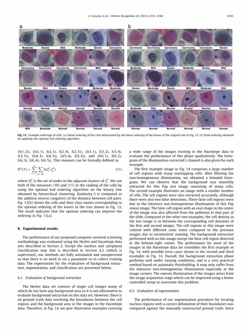
Fig. 13. Example orderings of cells. (a) Initial ordering of the cells determined by the linear ordering of the leaves of the original tree in Fig. 12. (b) Final ordering obtained

by applying the optimal leaf ordering algorithm.


fSð1;2Þg, fSð2;1Þ, Sð2;3Þ, Sð2;4Þ, Sð2;5Þg, fSð3;1Þ, Sð3;2Þ, Sð3;4Þ,Sð3;5Þg, fSð4;3Þ, Sð4;5Þg, fSð5;4Þ, Sð5;6Þg, and fSð6;1Þ, Sð6;2Þ,Sð6;3Þ, Sð6;4Þ, Sð6;5Þg. This measure can be formally defined as

DfðT Þ ¼

Xn

i ¼ 1

XjAAf

i

Sðzfi ,zfj Þ ð11Þ

where Afi is the set of nodes in the adjacent clusters of zfi . We use

both of the measures (10) and (11) in the ranking of the cells byusing the optimal leaf ordering algorithm on the binary treeobtained by hierarchical clustering. Similarity S is computed asthe additive inverse (negative) of the distance between cell pairs.Fig. 13(b) shows the cells and their class names corresponding tothe optimal ordering of the leaves in the tree shown in Fig. 12.The result indicates that the optimal ordering can improve theordering in Fig. 13(a).

6. Experimental results

The performance of our proposed computer-assisted screeningmethodology was evaluated using the Herlev and Hacettepe datasets described in Section 2. Except the nucleus and cytoplasmclassification step that is described in Section 4.2 (which issupervised), our methods are fully automated and unsupervisedso that there is no need to set a parameter or to collect trainingdata. The experiments for the evaluation of background extrac-tion, segmentation, and classification are presented below.

6.1. Evaluation of background extraction

The Herlev data set consists of single cell images many ofwhich do not have any background area so it is not informative toevaluate background extraction on this data set. However, there isno ground truth data involving the boundaries between the cellregions and the background area in the images in the Hacettepedata. Therefore, in Fig. 14, we give illustrative examples covering

a wide range of the images existing in the Hacettepe data toevaluate the performance of this phase qualitatively. The histo-gram of the illumination-corrected L channel is also given for eachexample.

The first example image in Fig. 14 comprises a large numberof cell regions with many overlapping cells. After filtering thenon-homogeneous illumination, we obtained a bimodal histo-gram. We can observe that the background was smoothlyextracted for this Pap test image consisting of many cells.The second example illustrates an image with a smaller numberof cells. The cell regions were also extracted accurately, althoughthere were also two false detections. These false cell regions weredue to the intensive non-homogeneous illumination of this Papsmear image. The false cell region with an oval shape in the centerof the image was also affected from the pollution in that part ofthe slide. Compared to the other two examples, the cell density inthe last image is in between the corresponding cell densities ofthe first and second images. The cell regions in this image werecolored with different color tones compared to the previousimages due to inconsistent staining. The background extractionperformed well on this image except the false cell region detectedat the bottom-right corner. The performance for most of theimages in the Hacettepe data set resembles the first example inFig. 14, with possible error cases shown in the second and thirdexamples in Fig. 14. Overall, the background extraction phaseperforms well under varying conditions, and is a very practicalmethod based on automatic thresholding. It may only suffer fromthe intensive non-homogeneous illumination especially at theimage corners. The uneven illumination of the images arises fromthe image acquisition stage which can be improved using a bettercontrolled setup to overcome this problem.

6.2. Evaluation of segmentation

The performance of our segmentation procedure for locatingnucleus regions with a correct delineation of their boundaries wascompared against the manually constructed ground truth. Since

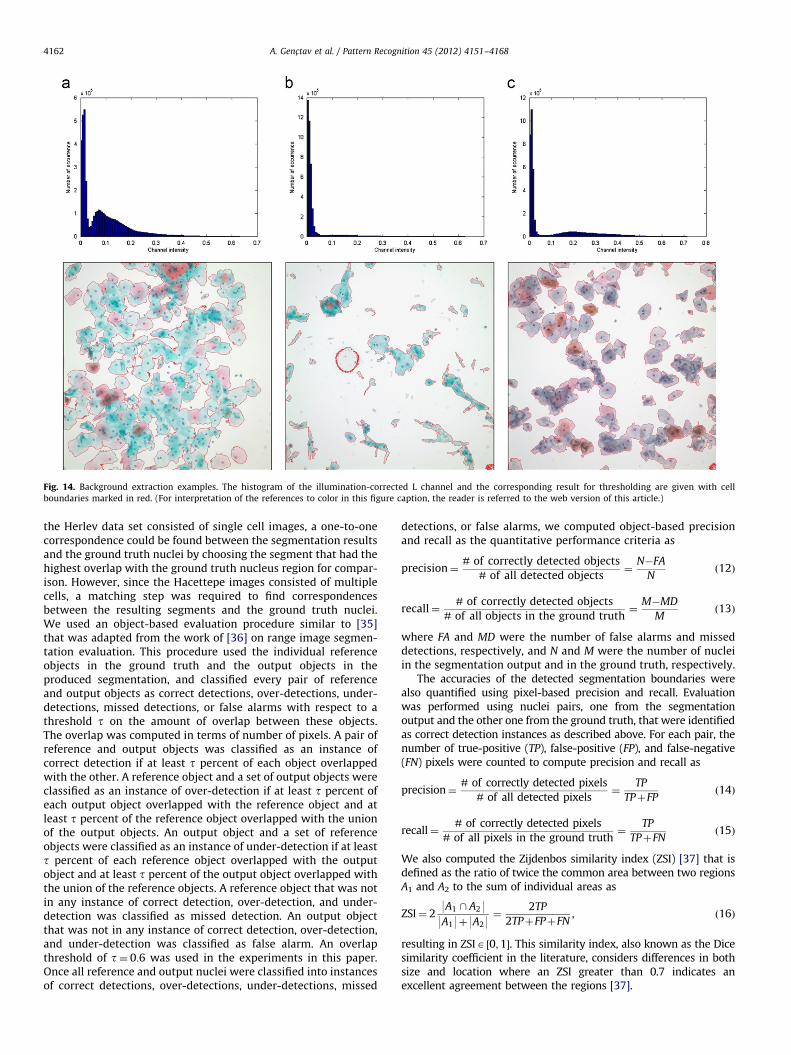
Fig. 14. Background extraction examples. The histogram of the illumination-corrected L channel and the corresponding result for thresholding are given with cell

boundaries marked in red. (For interpretation of the references to color in this figure caption, the reader is referred to the web version of this article.)


the Herlev data set consisted of single cell images, a one-to-onecorrespondence could be found between the segmentation resultsand the ground truth nuclei by choosing the segment that had thehighest overlap with the ground truth nucleus region for compar-ison. However, since the Hacettepe images consisted of multiplecells, a matching step was required to find correspondencesbetween the resulting segments and the ground truth nuclei.We used an object-based evaluation procedure similar to [35]that was adapted from the work of [36] on range image segmen-tation evaluation. This procedure used the individual referenceobjects in the ground truth and the output objects in theproduced segmentation, and classified every pair of referenceand output objects as correct detections, over-detections, under-detections, missed detections, or false alarms with respect to athreshold t on the amount of overlap between these objects.The overlap was computed in terms of number of pixels. A pair ofreference and output objects was classified as an instance ofcorrect detection if at least t percent of each object overlappedwith the other. A reference object and a set of output objects wereclassified as an instance of over-detection if at least t percent ofeach output object overlapped with the reference object and atleast t percent of the reference object overlapped with the unionof the output objects. An output object and a set of referenceobjects were classified as an instance of under-detection if at leastt percent of each reference object overlapped with the outputobject and at least t percent of the output object overlapped withthe union of the reference objects. A reference object that was notin any instance of correct detection, over-detection, and under-detection was classified as missed detection. An output objectthat was not in any instance of correct detection, over-detection,and under-detection was classified as false alarm. An overlapthreshold of t¼ 0:6 was used in the experiments in this paper.Once all reference and output nuclei were classified into instancesof correct detections, over-detections, under-detections, missed

detections, or false alarms, we computed object-based precisionand recall as the quantitative performance criteria as

precision¼# of correctly detected objects

# of all detected objects¼

N�FA

Nð12Þ

recall¼# of correctly detected objects

# of all objects in the ground truth¼

M�MD

Mð13Þ

where FA and MD were the number of false alarms and misseddetections, respectively, and N and M were the number of nucleiin the segmentation output and in the ground truth, respectively.

The accuracies of the detected segmentation boundaries werealso quantified using pixel-based precision and recall. Evaluationwas performed using nuclei pairs, one from the segmentationoutput and the other one from the ground truth, that were identifiedas correct detection instances as described above. For each pair, thenumber of true-positive (TP), false-positive (FP), and false-negative(FN) pixels were counted to compute precision and recall as

precision¼# of correctly detected pixels

# of all detected pixels¼

TP

TPþFPð14Þ

recall¼# of correctly detected pixels

# of all pixels in the ground truth¼

TP

TPþFNð15Þ

We also computed the Zijdenbos similarity index (ZSI) [37] that isdefined as the ratio of twice the common area between two regionsA1 and A2 to the sum of individual areas as

ZSI¼ 29A1 \ A299A19þ9A29

¼2TP

2TPþFPþFN, ð16Þ

resulting in ZSIA ½0;1�. This similarity index, also known as the Dicesimilarity coefficient in the literature, considers differences in bothsize and location where an ZSI greater than 0.7 indicates anexcellent agreement between the regions [37].

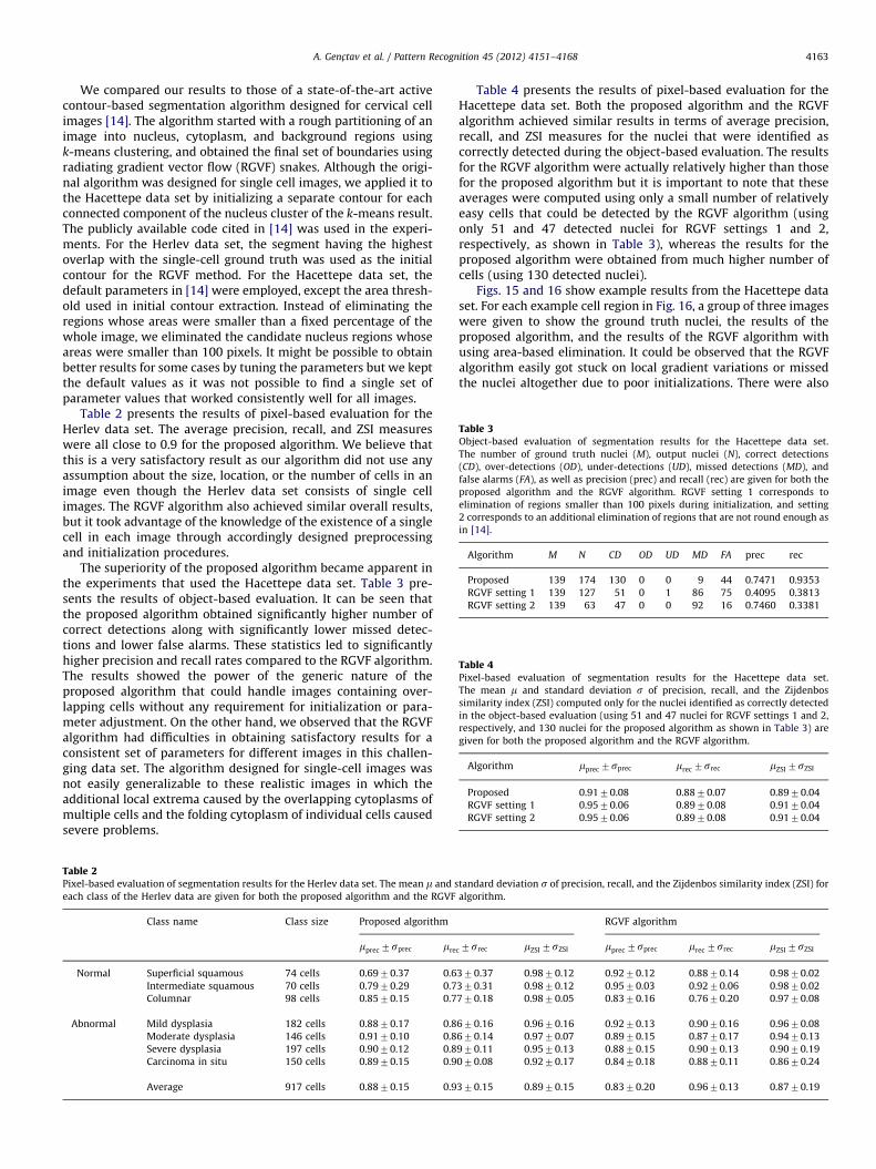
Table 3Object-based evaluation of segmentation results for the Hacettepe data set.

The number of ground truth nuclei (M), output nuclei (N), correct detections

(CD), over-detections (OD), under-detections (UD), missed detections (MD), and

false alarms (FA), as well as precision (prec) and recall (rec) are given for both the

proposed algorithm and the RGVF algorithm. RGVF setting 1 corresponds to

elimination of regions smaller than 100 pixels during initialization, and setting

2 corresponds to an additional elimination of regions that are not round enough as

in [14].

Algorithm M N CD OD UD MD FA prec rec

Proposed 139 174 130 0 0 9 44 0.7471 0.9353

RGVF setting 1 139 127 51 0 1 86 75 0.4095 0.3813

RGVF setting 2 139 63 47 0 0 92 16 0.7460 0.3381

Table 4Pixel-based evaluation of segmentation results for the Hacettepe data set.

The mean m and standard deviation s of precision, recall, and the Zijdenbos

similarity index (ZSI) computed only for the nuclei identified as correctly detected

in the object-based evaluation (using 51 and 47 nuclei for RGVF settings 1 and 2,

respectively, and 130 nuclei for the proposed algorithm as shown in Table 3) are

given for both the proposed algorithm and the RGVF algorithm.

Algorithm mprec 7sprec mrec 7srec mZSI 7sZSI

Proposed 0.9170.08 0.8870.07 0.8970.04

RGVF setting 1 0.9570.06 0.8970.08 0.9170.04

RGVF setting 2 0.9570.06 0.8970.08 0.9170.04


We compared our results to those of a state-of-the-art activecontour-based segmentation algorithm designed for cervical cellimages [14]. The algorithm started with a rough partitioning of animage into nucleus, cytoplasm, and background regions usingk-means clustering, and obtained the final set of boundaries usingradiating gradient vector flow (RGVF) snakes. Although the origi-nal algorithm was designed for single cell images, we applied it tothe Hacettepe data set by initializing a separate contour for eachconnected component of the nucleus cluster of the k-means result.The publicly available code cited in [14] was used in the experi-ments. For the Herlev data set, the segment having the highestoverlap with the single-cell ground truth was used as the initialcontour for the RGVF method. For the Hacettepe data set, thedefault parameters in [14] were employed, except the area thresh-old used in initial contour extraction. Instead of eliminating theregions whose areas were smaller than a fixed percentage of thewhole image, we eliminated the candidate nucleus regions whoseareas were smaller than 100 pixels. It might be possible to obtainbetter results for some cases by tuning the parameters but we keptthe default values as it was not possible to find a single set ofparameter values that worked consistently well for all images.

Table 2 presents the results of pixel-based evaluation for theHerlev data set. The average precision, recall, and ZSI measureswere all close to 0.9 for the proposed algorithm. We believe thatthis is a very satisfactory result as our algorithm did not use anyassumption about the size, location, or the number of cells in animage even though the Herlev data set consists of single cellimages. The RGVF algorithm also achieved similar overall results,but it took advantage of the knowledge of the existence of a singlecell in each image through accordingly designed preprocessingand initialization procedures.

The superiority of the proposed algorithm became apparent inthe experiments that used the Hacettepe data set. Table 3 pre-sents the results of object-based evaluation. It can be seen thatthe proposed algorithm obtained significantly higher number ofcorrect detections along with significantly lower missed detec-tions and lower false alarms. These statistics led to significantlyhigher precision and recall rates compared to the RGVF algorithm.The results showed the power of the generic nature of theproposed algorithm that could handle images containing over-lapping cells without any requirement for initialization or para-meter adjustment. On the other hand, we observed that the RGVFalgorithm had difficulties in obtaining satisfactory results for aconsistent set of parameters for different images in this challen-ging data set. The algorithm designed for single-cell images wasnot easily generalizable to these realistic images in which theadditional local extrema caused by the overlapping cytoplasms ofmultiple cells and the folding cytoplasm of individual cells causedsevere problems.

Table 2Pixel-based evaluation of segmentation results for the Herlev data set. The mean m and s

each class of the Herlev data are given for both the proposed algorithm and the RGVF

Class name Class size Proposed algorithm

mprec 7sprec mre

Normal Superficial squamous 74 cells 0.6970.37 0.6

Intermediate squamous 70 cells 0.7970.29 0.7

Columnar 98 cells 0.8570.15 0.7

Abnormal Mild dysplasia 182 cells 0.8870.17 0.8

Moderate dysplasia 146 cells 0.9170.10 0.8

Severe dysplasia 197 cells 0.9070.12 0.8

Carcinoma in situ 150 cells 0.8970.15 0.9

Average 917 cells 0.8870.15 0.9

Table 4 presents the results of pixel-based evaluation for theHacettepe data set. Both the proposed algorithm and the RGVFalgorithm achieved similar results in terms of average precision,recall, and ZSI measures for the nuclei that were identified ascorrectly detected during the object-based evaluation. The resultsfor the RGVF algorithm were actually relatively higher than thosefor the proposed algorithm but it is important to note that theseaverages were computed using only a small number of relativelyeasy cells that could be detected by the RGVF algorithm (usingonly 51 and 47 detected nuclei for RGVF settings 1 and 2,respectively, as shown in Table 3), whereas the results for theproposed algorithm were obtained from much higher number ofcells (using 130 detected nuclei).

Figs. 15 and 16 show example results from the Hacettepe dataset. For each example cell region in Fig. 16, a group of three imageswere given to show the ground truth nuclei, the results of theproposed algorithm, and the results of the RGVF algorithm withusing area-based elimination. It could be observed that the RGVFalgorithm easily got stuck on local gradient variations or missedthe nuclei altogether due to poor initializations. There were also

tandard deviation s of precision, recall, and the Zijdenbos similarity index (ZSI) for

algorithm.

RGVF algorithm

c 7srec mZSI 7sZSI mprec 7sprec mrec 7srec mZSI 7sZSI

370.37 0.9870.12 0.9270.12 0.8870.14 0.9870.02

370.31 0.9870.12 0.9570.03 0.9270.06 0.9870.02

770.18 0.9870.05 0.8370.16 0.7670.20 0.9770.08

670.16 0.9670.16 0.9270.13 0.9070.16 0.9670.08

670.14 0.9770.07 0.8970.15 0.8770.17 0.9470.13

970.11 0.9570.13 0.8870.15 0.9070.13 0.9070.19

070.08 0.9270.17 0.8470.18 0.8870.11 0.8670.24

370.15 0.8970.15 0.8370.20 0.9670.13 0.8770.19

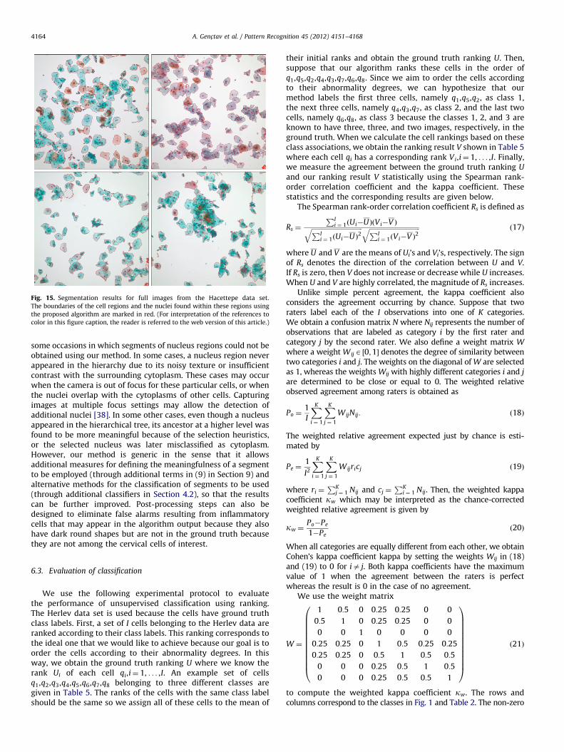
Fig. 15. Segmentation results for full images from the Hacettepe data set.

The boundaries of the cell regions and the nuclei found within these regions using

the proposed algorithm are marked in red. (For interpretation of the references to

color in this figure caption, the reader is referred to the web version of this article.)


some occasions in which segments of nucleus regions could not beobtained using our method. In some cases, a nucleus region neverappeared in the hierarchy due to its noisy texture or insufficientcontrast with the surrounding cytoplasm. These cases may occurwhen the camera is out of focus for these particular cells, or whenthe nuclei overlap with the cytoplasms of other cells. Capturingimages at multiple focus settings may allow the detection ofadditional nuclei [38]. In some other cases, even though a nucleusappeared in the hierarchical tree, its ancestor at a higher level wasfound to be more meaningful because of the selection heuristics,or the selected nucleus was later misclassified as cytoplasm.However, our method is generic in the sense that it allowsadditional measures for defining the meaningfulness of a segmentto be employed (through additional terms in (9) in Section 9) andalternative methods for the classification of segments to be used(through additional classifiers in Section 4.2), so that the resultscan be further improved. Post-processing steps can also bedesigned to eliminate false alarms resulting from inflammatorycells that may appear in the algorithm output because they alsohave dark round shapes but are not in the ground truth becausethey are not among the cervical cells of interest.

6.3. Evaluation of classification

We use the following experimental protocol to evaluatethe performance of unsupervised classification using ranking.The Herlev data set is used because the cells have ground truthclass labels. First, a set of I cells belonging to the Herlev data areranked according to their class labels. This ranking corresponds tothe ideal one that we would like to achieve because our goal is toorder the cells according to their abnormality degrees. In thisway, we obtain the ground truth ranking U where we know therank Ui of each cell qi,i¼ 1, . . . ,I. An example set of cellsq1,q2,q3,q4,q5,q6,q7,q8 belonging to three different classes aregiven in Table 5. The ranks of the cells with the same class labelshould be the same so we assign all of these cells to the mean of

their initial ranks and obtain the ground truth ranking U. Then,suppose that our algorithm ranks these cells in the order ofq1,q5,q2,q4,q3,q7,q6,q8. Since we aim to order the cells accordingto their abnormality degrees, we can hypothesize that ourmethod labels the first three cells, namely q1,q5,q2, as class 1,the next three cells, namely q4,q3,q7, as class 2, and the last twocells, namely q6,q8, as class 3 because the classes 1, 2, and 3 areknown to have three, three, and two images, respectively, in theground truth. When we calculate the cell rankings based on theseclass associations, we obtain the ranking result V shown in Table 5where each cell qi has a corresponding rank Vi,i¼ 1, . . . ,I. Finally,we measure the agreement between the ground truth ranking U

and our ranking result V statistically using the Spearman rank-order correlation coefficient and the kappa coefficient. Thesestatistics and the corresponding results are given below.

The Spearman rank-order correlation coefficient Rs is defined as

Rs ¼

PIi ¼ 1ðUi�UÞðVi�V ÞffiffiffiffiffiffiffiffiffiffiffiffiffiffiffiffiffiffiffiffiffiffiffiffiffiffiffiffiffiffiffiPI

i ¼ 1ðUi�UÞ2q ffiffiffiffiffiffiffiffiffiffiffiffiffiffiffiffiffiffiffiffiffiffiffiffiffiffiffiffiffiffiffiPI

i ¼ 1ðVi�V Þ2q ð17Þ

where U and V are the means of Ui’s and Vi’s, respectively. The signof Rs denotes the direction of the correlation between U and V.If Rs is zero, then V does not increase or decrease while U increases.When U and V are highly correlated, the magnitude of Rs increases.

Unlike simple percent agreement, the kappa coefficient alsoconsiders the agreement occurring by chance. Suppose that tworaters label each of the I observations into one of K categories.We obtain a confusion matrix N where Nij represents the number ofobservations that are labeled as category i by the first rater andcategory j by the second rater. We also define a weight matrix W

where a weight WijA ½0;1� denotes the degree of similarity betweentwo categories i and j. The weights on the diagonal of W are selectedas 1, whereas the weights Wij with highly different categories i and j

are determined to be close or equal to 0. The weighted relativeobserved agreement among raters is obtained as

Po ¼1

I

XK

i ¼ 1

XK

j ¼ 1

WijNij: ð18Þ

The weighted relative agreement expected just by chance is esti-mated by

Pe ¼1

I2

XK

i ¼ 1

XK

j ¼ 1

Wijricj ð19Þ

where ri ¼PK

j ¼ 1 Nij and cj ¼PK

i ¼ 1 Nij. Then, the weighted kappacoefficient kw which may be interpreted as the chance-correctedweighted relative agreement is given by

kw ¼Po�Pe

1�Peð20Þ

When all categories are equally different from each other, we obtainCohen’s kappa coefficient kappa by setting the weights Wij in (18)and (19) to 0 for ia j. Both kappa coefficients have the maximumvalue of 1 when the agreement between the raters is perfectwhereas the result is 0 in the case of no agreement.

We use the weight matrix

W ¼

1 0:5 0 0:25 0:25 0 0

0:5 1 0 0:25 0:25 0 0

0 0 1 0 0 0 0

0:25 0:25 0 1 0:5 0:25 0:25

0:25 0:25 0 0:5 1 0:5 0:5

0 0 0 0:25 0:5 1 0:5

0 0 0 0:25 0:5 0:5 1

0BBBBBBBBBBB@

1CCCCCCCCCCCA

ð21Þ

to compute the weighted kappa coefficient kw. The rows andcolumns correspond to the classes in Fig. 1 and Table 2. The non-zero

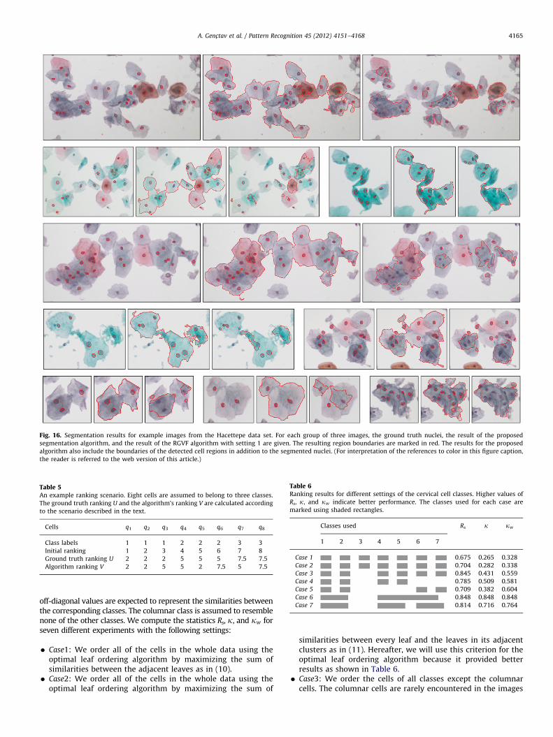
Table 5An example ranking scenario. Eight cells are assumed to belong to three classes.

The ground truth ranking U and the algorithm’s ranking V are calculated according

to the scenario described in the text.

Cells q1 q2 q3 q4 q5 q6 q7 q8

Class labels 1 1 1 2 2 2 3 3

Initial ranking 1 2 3 4 5 6 7 8

Ground truth ranking U 2 2 2 5 5 5 7.5 7.5

Algorithm ranking V 2 2 5 5 2 7.5 5 7.5

Fig. 16. Segmentation results for example images from the Hacettepe data set. For each group of three images, the ground truth nuclei, the result of the proposed

segmentation algorithm, and the result of the RGVF algorithm with setting 1 are given. The resulting region boundaries are marked in red. The results for the proposed

algorithm also include the boundaries of the detected cell regions in addition to the segmented nuclei. (For interpretation of the references to color in this figure caption,

the reader is referred to the web version of this article.)

Table 6Ranking results for different settings of the cervical cell classes. Higher values of

Rs, k, and kw indicate better performance. The classes used for each case are

marked using shaded rectangles.

Classes used Rs k kw

1 2 3 4 5 6 7

Case 1 0.675 0.265 0.328

Case 2 0.704 0.282 0.338

Case 3 0.845 0.431 0.559

Case 4 0.785 0.509 0.581

Case 5 0.709 0.382 0.604

Case 6 0.848 0.848 0.848

Case 7 0.814 0.716 0.764


off-diagonal values are expected to represent the similarities betweenthe corresponding classes. The columnar class is assumed to resemblenone of the other classes. We compute the statistics Rs, k, and kw forseven different experiments with the following settings:

�
Case1: We order all of the cells in the whole data using theoptimal leaf ordering algorithm by maximizing the sum ofsimilarities between the adjacent leaves as in (10). � Case2: We order all of the cells in the whole data using the
optimal leaf ordering algorithm by maximizing the sum of

similarities between every leaf and the leaves in its adjacentclusters as in (11). Hereafter, we will use this criterion for theoptimal leaf ordering algorithm because it provided betterresults as shown in Table 6.
� Case3: We order the cells of all classes except the columnar
cells. The columnar cells are rarely encountered in the images

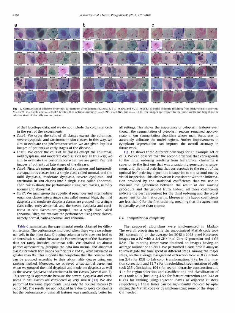
Fig. 17. Comparison of different orderings. (a) Random arrangement: Rs¼0.038, k¼�0:100, and kw ¼�0:054. (b) Initial ordering resulting from hierarchical clustering:

Rs¼0.771, k¼ 0:266, and kw ¼ 0:417. (c) Result of optimal ordering: Rs¼0.895, k¼ 0:466, and kw ¼ 0:614. The images are resized to the same width and height so the

relative sizes of the cells are not proper.


of the Hacettepe data, and we do not include the columnar cellsin the rest of the experiments.
� Case4: We order the cells of all classes except the columnar,
severe dysplasia, and carcinoma in situ classes. In this way, weaim to evaluate the performance when we are given Pap testimages of patients at early stages of the disease.
� Case5: We order the cells of all classes except the columnar,
mild dysplasia, and moderate dysplasia classes. In this way, weaim to evaluate the performance when we are given Pap testimages of patients at late stages of the disease.
� Case6: First, we group the superficial squamous and intermedi-
ate squamous classes into a single class called normal, and themild dysplasia, moderate dysplasia, severe dysplasia, andcarcinoma in situ classes into a single class called abnormal.Then, we evaluate the performance using two classes, namelynormal and abnormal.
� Case7: We again group the superficial squamous and intermediate
squamous classes into a single class called normal. Next, the milddysplasia and moderate dysplasia classes are grouped into a singleclass called early-abnormal, and the severe dysplasia and carci-noma in situ classes are grouped into a single class calledabnormal. Then, we evaluate the performance using three classes,namely normal, early-abnormal, and abnormal.

Table 6 summarizes the experimental results obtained for differ-ent settings. The performance improved when there were no colum-nar cells in the input data. Dropping columnar cells does not lead toan unrealistic situation, because the Pap test images of the Hacettepedata set rarely included columnar cells. We obtained an almostperfect agreement by grouping the data into normal and abnormalclasses for which both kappa coefficients k and kw were calculated asgreater than 0.8. This supports the conjecture that the cervical cellscan be grouped according to their abnormality degree using ourranking method. Moreover, we achieved a substantial agreementwhen we grouped the mild dysplasia and moderate dysplasia as wellas the severe dysplasia and carcinoma in situ classes (cases 6 and 7).This setting is appropriate because the severe dysplasia and carci-noma in situ classes are considered as very similar [39]. We alsoperformed the same experiments using only the nucleus features (9out of 14). The results are not included here due to space constraintsbut the performance of using all features was significantly better for

all settings. This shows the importance of cytoplasm features eventhough the segmentation of cytoplasm regions remained approxi-mate in our segmentation algorithm whose main focus was toaccurately delineate the nuclei regions. Further improvements incytoplasm segmentation can improve the overall accuracy infuture work.

Fig. 17 shows three different orderings for an example set ofcells. We can observe that the second ordering that correspondsto the initial ordering resulting from hierarchical clustering issuperior to the first one that was a randomly generated arrange-ment, and the third ordering that corresponds to the result of theoptimal leaf ordering algorithm is superior to the second one byvisual inspection. This observation is consistent with the informa-tion provided by the statistical coefficients that we use tomeasure the agreement between the result of our rankingprocedure and the ground truth. Indeed, all three coefficientsindicate the best agreement for the third ordering and the worstagreement for the first ordering. Moreover, the kappa coefficientsare less than 0 for the first ordering, meaning that the agreementis actually worse than chance.

6.4. Computational complexity

The proposed algorithms were implemented in Matlab.The overall processing using the unoptimized Matlab code took261 seconds (s) on the average for 2048�2048 pixel Hacettepeimages on a PC with a 3.4 GHz Intel Core i7 processor and 4 GBRAM. The running times were obtained on images having anaverage number of 45 cells. We performed a code profile analysisto investigate the time spent in different steps. Among the majorsteps, on the average, background extraction took 20.8 s (includ-ing 2.4 s for RGB to Lab color transformation, 4.7 s for illumina-tion correction, and 13.7 s for thresholding), segmentation of cellstook 235 s (including 194 s for region hierarchy construction and41 s for region selection and classification), and classification ofcells took 4.9 s (including 4.5 s for feature extraction and 0.42 or0.39 s for ranking using adjacent leaves or adjacent clusters,respectively). These times can be significantly reduced by opti-mizing the Matlab code or by implementing some of the steps inC if needed.


7. Conclusions

We presented a computer-assisted screening procedure thataimed to help the grading of Pap smear slides by sorting the cellsaccording to their abnormality degrees. The procedure consisted oftwo main tasks. The first task, segmentation, involved morphologicaloperations and automatic thresholding for isolating the cell regionsfrom the background, a hierarchical segmentation algorithm thatused homogeneity and circularity criteria for partitioning these cells,and a binary classifier for separating the nuclei from cytoplasmwithin the cell regions. The second task, classification, ranked thecells based on their feature characteristics computed from the nucleiand cytoplasm regions. The ranking was generated via linearization ofthe leaves of a binary tree that was constructed using hierarchicalclustering. Experiments using two data sets showed that the pro-posed approach could produce accurate segmentation and classifica-tion of cervical cells in images having inconsistent staining, poorcontrast, and overlapping cells. Furthermore, both the segmentationand the classification algorithms are parameter-free and generic sothat additional criteria can easily be incorporated to improve theidentification of different cell types without any requirement fortraining examples.

Our main focus in this paper was to correctly delineate theindividual nuclei while assuming that the overlapping cytoplasmareas were shared by different cells. We observed that, in additionto nuclei features, using the cytoplasm features extracted fromthis approximate segmentation resulted in an increase in theclassification accuracy. Therefore, future work will include addi-tional steps for improving the segmentation of nuclei and cyto-plasm areas within overlapping cell groups. We believe that moreaccurate features computed from the improved cytoplasm regionswill also improve the grading performance.

Acknowledgment

This work was supported in part by the TUBITAK CAREERGrant 104E074.

References

[1] World Health Organization, Comprehensive Cervical Cancer Control: A Guideto Essential Practice, 2006.

[2] H.Z. Noorani, C. Arratoon, A. Hall, Assessment of Techniques for CervicalCancer Screening, Technical Report CCOHTA Report 1997: 2E, CanadianCoordinating Office for Health Technology Assessment (May 1997).

[3] E. Bengtsson, Computerized cell image analysis: past, present, and future,in: Proceedings of 13th Scandinavian Conference on Image Analysis, 2003,pp. 395–407.

[4] E. Bengtsson, Recognizing signs of malignancy—the quest for computerassisted cancer screening and diagnosis systems, in: IEEE InternationalConference on Computational Intelligence and Computing Research, 2010.

[5] P. Bamford, B. Lovell, Unsupervised cell nucleus segmentation with activecontours, Signal Processing 71 (2) (1998) 203–213.

[6] H.-S. Wu, J. Barba, J. Gil, A parametric fitting algorithm for segmentation of cellimages, IEEE Transactions on Biomedical Engineering 45 (3) (1998) 400–408.

[7] S.-F. Yang-Mao, Y.-K. Chan, Y.-P. Chu, Edge enhancement nucleus andcytoplasm contour detector of cervical smear images, IEEE Transactions onSystems, Man, and Cybernetics Part B: Cybernetics 38 (2) (2008) 353–366.

[8] M.-H. Tsai, Y.-K. Chan, Z.-Z. Lin, S.-F. Yang-Mao, P.-C. Huang, Nucleus andcytoplasm contour detector of cervical smear image, Pattern RecognitionLetters 29 (9) (2008) 1441–1453.

[9] I. Dagher, K.E. Tom, WaterBalloons: a hybrid watershed balloon snakesegmentation, Image and Vision Computing 26 (7) (2008) 905–912.

[10] P.-W. Huang, Y.-H. Lai, Effective segmentation and classification for HCCbiopsy images, Pattern Recognition 43 (4) (2010) 1550–1563.

[11] N.M. Harandi, S. Sadri, N.A. Moghaddam, R. Amirfattahi, An automatedmethod for segmentation of epithelial cervical cells in images of ThinPrep,Journal of Medical Systems 34 (6) (2010) 1043–1058.

[12] M.E. Plissiti, C. Nikou, A. Charchanti, Automated detection of cell nuclei in Pap

smear images using morphological reconstruction and clustering, IEEE Transac-

tions on Information Technology in Biomedicine 15 (2) (2011) 233–241.[13] M.E. Plissiti, C. Nikou, A. Charchanti, Combining shape, texture and intensity

features for cell nuclei extraction in Pap smear images, Pattern Recognition

Letters 32 (6) (2011) 838–853.[14] K. Li, Z. Lu, W. Liu, J. Yin, Cytoplasm and nucleus segmentation in cervical

smear images using Radiating GVF snake, Pattern Recognition 45 (4) (2012)

1255–1264.[15] Y. Marinakis, G. Dounias, J. Jantzen, Pap smear diagnosis using a hybrid

intelligent scheme focusing on genetic algorithm based feature selection and

nearest neighbor classification, Computers in Biology and Medicine 39 (1)

(2009) 69–78.[16] A. Kale, S. Aksoy, S. Onder, Cell nuclei segmentation in pap smear test images,

in: Proceedings of 17th IEEE Signal Processing and Communications Applica-

tions, Antalya, Turkey, 2009.[17] S. Ali, A. Madabhushi, Active contour for overlap resolution using watershed

based initialization (ACOReW): applications to histopathology, in: IEEE

International Symposium on Biomedical Imaging: From Nano to Macro,

2011, pp. 614–617.[18] I. Vanhamel, I. Pratikakis, H. Sahli, Multiscale gradient watersheds of color

images, IEEE Transactions on Image Processing 12 (6) (2003) 617–626.[19] Y.-Y. Wang, Y.-N. Sun, C.-C. K. Lin, M.-S. Ju, Nerve cell segmentation via

multi-scale gradient watershed hierarchies, in: 28th Annual International

Conference of the IEEE Engineering in Medicine and Biology Society, 2006,

pp. 4310–4313.[20] M.A.G. de Carvalho, R.deA. Lotufo, M. Couprie, Morphological segmentation

of yeast by image analysis, Image and Vision Computing 25 (1) (2007) 34–39.[21] R.F. Walker, P. Jackway, B. Lovell, I. D. Longstaff, Classification of cervical cell

nuclei using morphological segmentation and textural feature extraction,

in: Proceedings of 1994 Second Australian and New Zealand Conference on

Intelligent Information Systems, 1994, pp. 297–301.[22] Y.-Y. Chou, L.G. Shapiro, A hierarchical multiple classifier learning algorithm,

Pattern Analysis and Applications 6 (2) (2003) 150–168.[23] J. Zhang, Y. Liu, Cervical cancer detection using svm based feature screening,

in: International Conference on Medical Image Computing and Computer

Aided Intervention, vol. 2, 2004, pp. 873–880.[24] H.C. Kitchener, R. Blanks, G. Dunn, L. Gunn, M. Desai, R. Albrow, J. Mather,

D.N. Rana, H. Cubie, C. Moore, R. Legood, A. Gray, S. Moss, Automation-

assisted versus manual reading of cervical cytology (MAVARIC): a rando-

mised controlled trial, Oncology 12 (1) (2011) 56–64.[25] E. Martin, Pap-smear Classification, Master’s Thesis, Technical University of

Denmark, Oersted-DTU, Automation, Lyngby, Denmark, 2003.[26] P. Soille, Morphological Image Analysis, second ed., Springer, 2002.[27] J. Kittler, J. Illingworth, Minimum error thresholding, Pattern Recognition 19

(1) (1986) 41–47.[28] A. Kale, S. Aksoy, Segmentation of cervical cell images, in: Proceedings of

20th IAPR International Conference on Pattern Recognition, Istanbul, Turkey,

2010, pp. 2399–2402.[29] E.R. Dougherty, R.A. Lotufo, Hands-on Morphological Image Processing, SPIE

Publications, 2003.[30] R.M. Haralick, L.G. Shapiro, Computer and Robot Vision, Addison-Wesley, 1992.[31] W.H. Press, S.A. Teukolsky, W.T. Vetterling, B.P. Flannery, Numerical Recipes:

The Art of Scientific Computing, third ed., Cambridge University Press, 2007.[32] R.O. Duda, P.E. Hart, D.G. Stork, Pattern Classification, John Wiley & Sons, Inc.,

2000.[33] H.G. Akcay, S. Aksoy, Automatic detection of geospatial objects using multi-

ple hierarchical segmentations, IEEE Transactions on Geoscience and Remote

Sensing 46 (7) (2008) 2097–2111.[34] Z. Bar-Joseph, D.K. Gifford, T.S. Jaakkola, Fast optimal leaf ordering for

hierarchical clustering, Bioinformatics 17 (2001) S22–S29.[35] B. Ozdemir, S. Aksoy, S. Eckert, M. Pesaresi, D. Ehrlich, Performance measures

for object detection evaluation, Pattern Recognition Letters 31 (10) (2010)

1128–1137.[36] A. Hoover, G. Jean-Baptiste, X. Jiang, P.J. Flynn, H. Bunke, D.B. Goldgof,

K. Bowyer, D.W. Eggert, A. Fitzgibbon, R.B. Fisher, An experimental compar-

ison of range image segmentation algorithms, IEEE Transactions on Pattern

Analysis and Machine Intelligence 18 (7) (1996) 673–689.[37] A.P. Zijdenbos, B.M. Dawant, R.A. Margolin, A.C. Palmer, Morphometric

analysis of white matter lesions in MR images: method and validation, IEEE

Transactions on Medical Imaging 13 (4) (1994) 716–724.[38] R.W. Mackin Jr., B. Roysam, J.N. Turner, Adaptive 3-D segmentation

algorithms for microscope images using local in-focus, and contrast features:

application to Pap smears, in: IEEE International Conference on Image

Processing, vol. 3, 1995, pp. 160–163.[39] J. Norup, Classification of Pap-smear Data by Transductive Neuro-fuzzy

Methods, Master’s Thesis, Technical University of Denmark, Oersted-DTU,

Automation, Lyngby, Denmark, 2005.


Aslı Genc-tav received the B.S. degree from the Middle East Technical University (METU), Ankara, Turkey, in 2007. She received the M.S. degree from the Bilkent University,Ankara, Turkey, in 2010. She is currently a Ph.D. candidate at the Department of Computer Engineering at METU. Her research interests include computer vision.

Selim Aksoy received the B.S. degree from the Middle East Technical University, Ankara, Turkey, in 1996 and the M.S. and Ph.D. degrees from the University of Washington,Seattle, in 1998 and 2001, respectively. Since 2004, he has been an Assistant Professor at the Department of Computer Engineering, Bilkent University, Ankara. His researchinterests include computer vision, statistical and structural pattern recognition with applications to remote sensing, medical imaging, and multimedia data analysis. He isan Associate Editor of Pattern Recognition Letters.

Sevgen Onder finished his pathology residency at the Hacettepe University School of Medicine in 2003. Currently he works in the same department as an AssistantProfessor. His major interests are cytopathology and pulmonary pathology. In addition to morphology, he is also interested in molecular pathology and utilization ofadvanced technology for diagnostic purpose.

Unsupervised segmentation and classification of cervical...

Documents

Transcript of Unsupervised segmentation and classification of cervical...