Unreplicated ANOVA designs

Block and repeated measures analyses

Gerry Quinn & Mick Keough, 1998Do not copy or distribute without permission of authors.

Blocking

• Aim:– Reduce unexplained variation, without

increasing size of experiment.

• Approach:– Group experimental units (“replicates”) into

blocks.– Blocks usually spatial units, 1 experimental

unit from each treatment in each block.

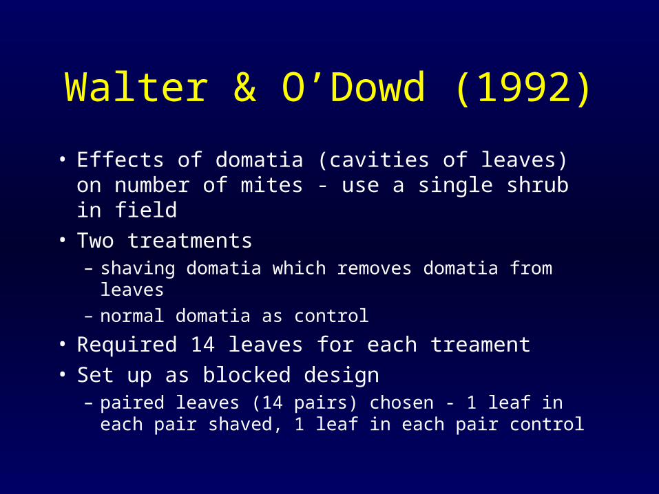
Walter & O’Dowd (1992)

• Effects of domatia (cavities of leaves) on number of mites - use a single shrub in field

• Two treatments– shaving domatia which removes domatia from leaves

– normal domatia as control

• Required 14 leaves for each treament

• Set up as completely randomised design– 28 leaves randomly allocated to each of 2 treatments

Completely randomised design

Control leaves Shaved domatia leaves

Completely randomised ANOVANo. of treatments or groups for factor A = a (2 for domatia), number of replicates = n (14 pairs of leaves)

Source general df example df

Factor A a-1 1Residual a(n-1) 26

Total an-1 27

Walter & O’Dowd (1992)

• Effects of domatia (cavities of leaves) on number of mites - use a single shrub in field

• Two treatments– shaving domatia which removes domatia from leaves– normal domatia as control

• Required 14 leaves for each treament• Set up as blocked design

– paired leaves (14 pairs) chosen - 1 leaf in each pair shaved, 1 leaf in each pair control

1 block

Control leaves Shaved domatia leaves

Rationale for blocking

• Micro-temperature, humidity, leaf age, etc. more similar within block than between blocks

• Variation in DV (mite number) between leaves within block (leaf pair) < variation between leaves between blocks

Rationale for blocking

• Some of unexplained (residual) variation in DV from completely randomised design now explained by differences between blocks

• More precise estimate of treatment effects than if leaves were chosen completely randomly from shrub

Null hypotheses

• No effect of treatment (Factor A)– HO: 1 = 2 = 3 = ... =

– HO: 1 = 2 = 3 = ... = 0 (i = i - )

– no effect of shaving domatia, pooling blocks

• No effect of blocks (?)– no difference between blocks (leaf pairs),

pooling treatments

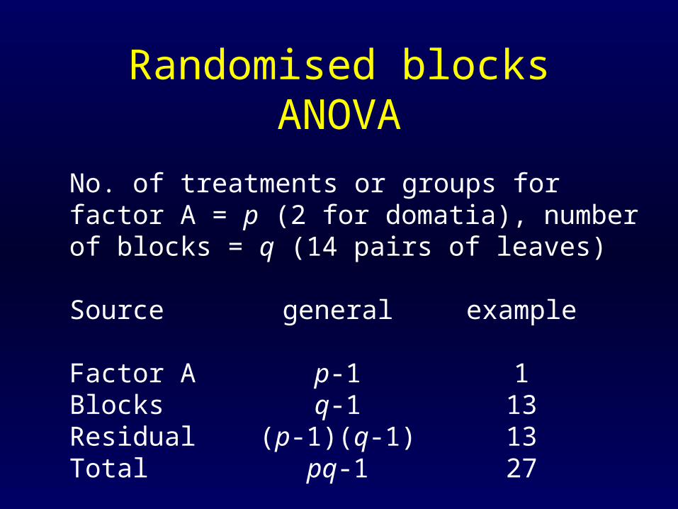
No. of treatments or groups for factor A = p (2 for domatia), number of blocks = q (14 pairs of leaves)

Source general example

Factor A p-1 1Blocks q-1 13Residual (p-1)(q-1) 13Total pq-1 27

Randomised blocks ANOVA

Randomised block ANOVA

• Randomised block ANOVA is 2 factor factorial design– BUT no replicates within each cell

(treatment-block combination), i.e. unreplicated 2 factor design

– No measure of within-cell variation– No test for treatment by block interaction

If factor A is fixed and Blocks (B) are random:

MSA (Treatments) 2 + 2 + (i)2/a-1

MSBlocks 2 + n2

MSResidual 2 + 2

Cannot separately estimate 2 and 2:

• no replicates within each block-treatment combination.

Expected mean squares

Null hypotheses

• If HO of no effects of factor A is true:

– all i’s = 0 and all ’s are the same

– then F-ratio MSA / MSResidual 1.

• If HO of no effects of factor A is false:

– then F-ratio MSA / MSResidual > 1.

Walter & O’Dowd (1992)

Factor A (treatment - shaved and unshaved domatia) - fixed, Blocks (14 pairs of leaves) - random:

Source df MS F P

Treatment 1 31.34 11.32 0.005Block 13 1.77 0.64 0.784 ??Residual 13 2.77

Randomised block vs completely randomised designs

• Total number of replicates is same in both designs– 28 leaves in total for domatia experiment

• Block designs rearrange spatial pattern of replicates into blocks:– “replicates” in block designs are the blocks

• Test of factor A (treatments) has fewer df in block design:– reduced power of test

Randomised block vs completely randomised designs

• MSResidual smaller in block design if blocks explain some of variation in DV:– increased power of test

• If decrease in MSResidual (unexplained variation) outweighs loss of df, then block design is better:– when blocks explain a lot of variation in DV

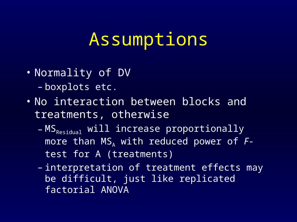
Assumptions

• Normality of DV– boxplots etc.

• No interaction between blocks and treatments, otherwise– MSResidual will increase proportionally more than

MSA with reduced power of F-test for A (treatments)

– interpretation of treatment effects may be difficult, just like replicated factorial ANOVA

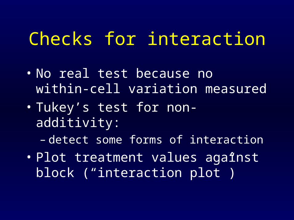
Checks for interaction

• No real test because no within-cell variation measured

• Tukey’s test for non-additivity:– detect some forms of interaction

• Plot treatment values against block (“interaction plot”)

Interaction plots

DV

Block

DV

No interaction

Interaction

Repeated measures designs

• A common experimental design in biology (and psychology)

• Different treatments applied to whole experimental units (called “subjects”)

or

• Experimental units recorded through time

Repeated measures designs

• The effect of four experimental drugs on heart rate of rats:– five rats used– each rat receives all four drugs in random

order

• Time as treatment factor is most common use of repeated measures designs in biology

Driscoll & Roberts (1997)

• Effect of fuel-reduction burning on frogs• Six drainages:

– blocks or subjects

• Three treatments (times):– pre-burn, post-burn 1, post-burn 2

• DV:– difference between no. calling males on

paired burnt-unburnt sites at each drainage

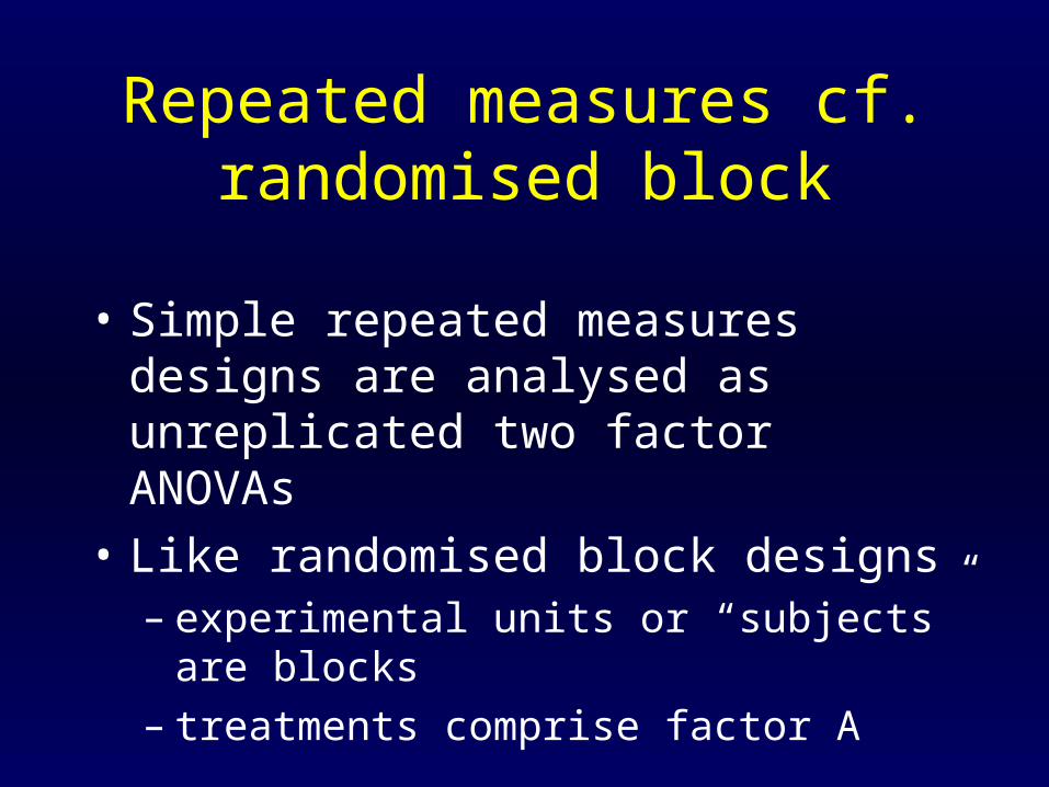
Repeated measures cf. randomised block

• Simple repeated measures designs are analysed as unreplicated two factor ANOVAs

• Like randomised block designs– experimental units or “subjects” are blocks– treatments comprise factor A

Randomised blockSource dfTreatments p-1Blocks q-1Residual (p-1)(q-1)Total pq-1

Repeated measuresSource dfBetween “subjects” q-1Within subjects

Treatments p-1Residual (p-1)(q-1)

Total pq-1

Driscoll & Roberts (1997)

Source df MS F P

Betweendrainages 5 1046.28

Withindrainages 12 443.33

Years 2 246.78 6.28 0.017Residual 10 196.56

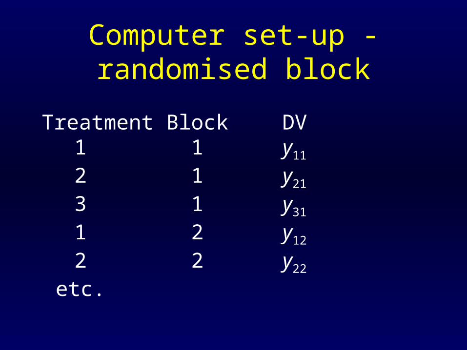
Treatment Block DV1 1 y11

2 1 y21

3 1 y31

1 2 y12

2 2 y22

etc.

Computer set-up - randomised block

Computer set-up - repeated measures

Subject Time 1 Time 2 Time 3 etc.1 y11 y21 y31

2 y12 y22 y32

3 y13 y23 y33

Both analyses produce identical results

Sphericity assumption

Block Treat 1 Treat 2 Treat 3 etc.

1 y11 y21 y31

2 y12 y22 y32

3 y13 y23 y33

etc.

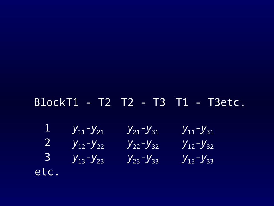
Block T1 - T2 T2 - T3 T1 - T3 etc.

1 y11-y21 y21-y31 y11-y31

2 y12-y22 y22-y32 y12-y32

3 y13-y23 y23-y33 y13-y33

etc.

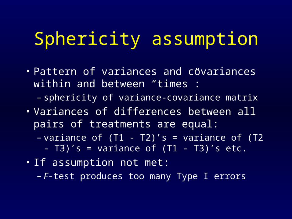
Sphericity assumption

• Pattern of variances and covariances within and between “times”:– sphericity of variance-covariance matrix

• Variances of differences between all pairs of treatments are equal: – variance of (T1 - T2)’s = variance of (T2 - T3)’s =

variance of (T1 - T3)’s etc.

• If assumption not met:– F-test produces too many Type I errors

Sphericity assumption

• Applies to randomised block and repeated measures designs

• Epsilon () statistic indicates degree to which sphericity is not met– further is from 1, more variances of treatment

differences are different

• Two versions of – Greenhouse-Geisser – Huyhn-Feldt

Dealing with non-sphericity

If not close to 1 and sphericity not met, there are 2 approaches:– Adjusted ANOVA F-tests

• df for F-tests from ANOVA adjusted downwards (made more conservative) depending on value

– Multivariate ANOVA (MANOVA)• treatments considered as multiple DVs in

MANOVA

Sphericity assumption

• Assumption of sphericity probably OK for randomised block designs:– treatments randomly applied to experimental

units within blocks

• Assumption of sphericity probably also OK for repeated measures designs:– if order each “subject” receives each

treatment is randomised (eg. rats and drugs)

Sphericity assumption

• Assumption of sphericity probably not OK for repeated measures designs involving time:– because DV for times closer together more

correlated than for times further apart– sphericity unlikely to be met– use Greenhouse-Geisser adjusted tests or

MANOVA

Examples from literature

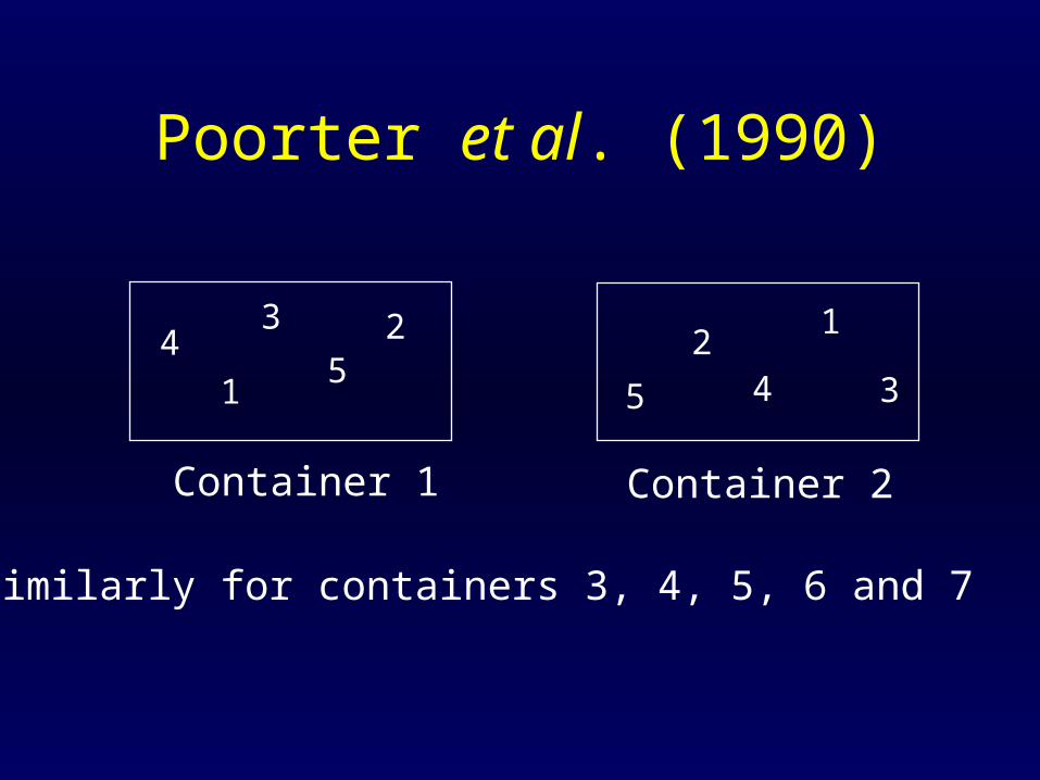
Poorter et al. (1990)

• Growth of five genotypes (3 fast and 2 slow) of Plantago major (a dicot plant called ribwort)

• One replicate seedling of each genotype was placed in each of 7 plastic containers in growth chamber

• Genotypes (1, 2, 3, 4, 5) are treatments, containers are blocks, DV is total plant weight (g) after 12 days

Poorter et al. (1990)

1

234

5

12

345

Container 1 Container 2

Similarly for containers 3, 4, 5, 6 and 7

Source df MS F P

Genotype 4 0.125 3.81 0.016Block 6 0.118Residual 24 0.033Total 34

Conclusions:• Large variation between containers (= blocks) so

block design probably better than completely randomised design

• Significant difference in growth between genotypes

Robles et al. (1995)

• Effect of increased mussel (Mytilus spp.) recruitment on seastar numbers

• Two treatments: 30-40L of Mytilus (0.5-3.5cm long) added, no Mytilus added

• Four matched pairs of mussel beds chosen, each pair = block

• Treatments randomly assigned to mussel beds within a pair

• DV is % change in seastar numbers

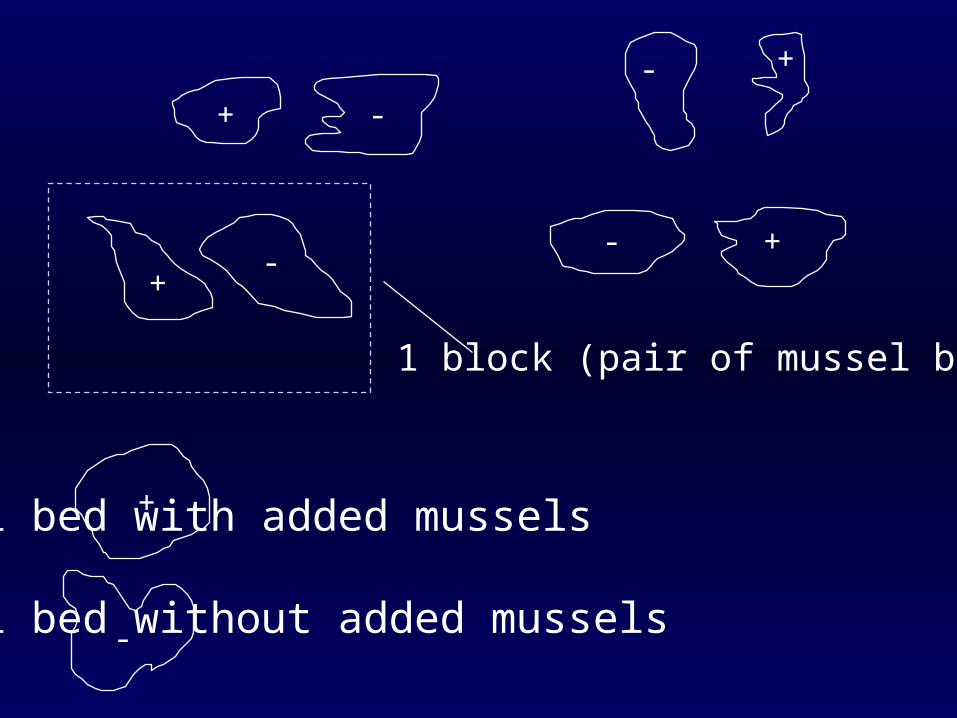
mussel bed with added mussels

mussel bed without added mussels

+ -

- +

- ++

-

1 block (pair of mussel beds)

+

-

Source df MS F P

Blocks 3 62.82Treatment 1 5237.21 45.50 0.007Residual 3 115.09

Conclusions:• Relatively little variation between blocks so a

completely randomised design probably better because treatments would have 1,6 df

• Significant treatment effect - more seastars where mussels added