Unraveling a puzzle: The case of Value Line timeliness ... · been exploiting the price momentum...

Unraveling a puzzle: The case of Value Line

timeliness rank upgrades *

Nandu Nayar Lehigh University [email protected]

610-758-4161

Ajai Singh Case Western Reserve University

[email protected] 216-368-0802

Wen Yu University of St. Thomas

[email protected] 651-962-5428

This draft: November 22, 2007

Preliminary Please do not cite without authors’ permission

* We are especially grateful to Dan Collins, Srini Krishnamurthy, CNV Krishnan, and Leonardo Madureira for helpful suggestions and to Anne Anderson, Christa Bouwman, Cynthia Campbell, Rick Carter, Hong Chen, Arnie Cowan, Rick Dark, Anand Vijh and the seminar participants at Case Western Reserve University, Iowa Sate University, Louisiana State University and the University of Iowa for their comments. The authors alone are responsible for any remaining errors. We thank Thomson Financial Services, Inc. for the I/B/E/S data provided as part of a broad academic program to encourage earnings expectation research, and Value Line Investment Survey (especially Sam Eisenstadt and Hassan Davis) for providing data on rank changes. Nayar is grateful for financial support from the Hans Julius Bär Endowed Chair.

1

Unraveling a puzzle: The case of Value Line timeliness rank upgrades

Abstract

We examine a sample of Value Line’s timeliness rank upgrades that occur immediately

following earnings announcements and find that the pre-event price momentum has

significant incremental explanatory power for the post-event drift, after controlling for

the level of earnings surprise. Therefore, the drift following Value Line’s timeliness

upgrades of the stocks that it covers cannot be construed as a mere manifestation of the

post-earnings announcement drift. Instead, these findings indicate that Value Line has

been exploiting the price momentum effect for decades. Black (1973) had clearly stated

that they do but his assertion has never been checked before to resolve the puzzling drift

following Value Line rank upgrades.

2

Unraveling a puzzle: The case of Value Line timeliness rank upgrades

The Value Line Investment Survey is a popular investment advisory service,

covering approximately 1,700 of the larger firms listed across various stock exchanges

and Nasdaq. Among other stock-related information, Value Line provides ‘timeliness

ranks’ for the stocks it covers, which range from one (best) to five (worst). The

timeliness ranks are purportedly a projection of a stock’s anticipated performance over

the following 12 months. A number of empirical studies have examined Value Line’s

timeliness ranks and documented an intriguing set of results; higher ranked stocks have a

superior performance to those lower down in Value Line’s timeliness ranking scale. The

persistence in stock-price drift following Value Line’s timeliness rank upgrades has also

been a puzzle. The phenomenon, entitled the Value Line Enigma, has endured across

studies employing different sample periods and methods; and these results are regarded

as a challenge to market efficiency.1

In this paper, we examine the stock price drift pursuant to a Value Line timeliness

rank upgrade where, by design, the upgrades follow an earnings announcement date. We

take our cue from Black (1973). In his well-cited letter to the Financial Analysts Journal

editor, Black (1973) clearly enunciates that Value Line uses price momentum as one of

the factors to assign ranks to stocks. However, prior research has not examined the

importance of pre-event price momentum in explaining the drift associated with Value

Line’s stock upgrades. We examine the event-period around the earnings announcement

date and the Value Line timeliness rank upgrade date and provide evidence that the pre-

event price momentum of the upgraded stocks is a significant explanatory variable for the

drift in stock prices following an upgrade. .

Despite its fairly recent discovery in academic studies, price momentum is a long

enduring empirical regularity. It is the tendency of stock prices to drift with a positive

correlation to past abnormal returns over 3- to 12-month holding periods. Jegadeesh and

1 See Holloway (1981), Copeland and Mayers (1982), Huberman and Kandel (1987).

3

Titman (1993) were the first to document the momentum effect.2 Fama and French

(2006) regard the momentum regularity as a ‘premier anomaly’ which is not consistent

with the tenets of market efficiency.

The post-earnings announcement drift is another observable anomaly that has

been studied extensively; it is the short-term tendency of stocks to drift in the same

direction as a recently announced earnings surprise.3 In an earlier paper, Affleck-Graves

and Mendenhall (1992) suggest that Value Line rank revisions are made in response to

recent earnings surprises, and that the Value Line Enigma is a mere manifestation of the

post-earnings announcement drift phenomenon. Affleck-Graves and Mendenhall (1992)

report that once the earnings surprise is controlled for, the post-upgrade drift (abnormal

returns following their upgrade) across Value Line stocks is no longer significant .

Affleck-Graves and Mendenhall conclude that ‘…Value Line reacts to, rather than

anticipates, earnings announcements.’ (p. 84)

The fact that the level of earnings surprise is a significant determinant of the post-

upgrade drift appears to be supported by Value Line’s own statement regarding its

weekly list of notable rank upgrades. Value Line states:

“We include mostly rank changes caused by fundamentals such as new earnings reports. Even when a significant change in earnings momentum has been forecast, the stock’s rank will not be affected until the actual results, confirming that forecast, are reported.”

Prima facie the above statement from Value Line indeed supports the conclusions drawn

by Affleck-Graves and Mendenhall (1992). However, the statement raises some

interesting questions. Does Value Line merely piggy-back on the drift following publicly

disclosed abnormal earnings reports? And if it does, then why does Value Line publicize

and openly disclose a proprietary trade secret? We address these issues in an attempt to

unravel the Value Line Enigma.

We find that the post-earnings announcement drift is positively related to the level

of earnings surprise for the Value Line upgraded stocks. In addition, we find that post-

2 Jegadeesh and Titman (1993) describe it as an investment strategy that consists of buying stocks that have performed well and selling stocks that have performed poorly in the past. The trading strategy generates significant positive returns over future 3- to 12-month holding periods. 3 See Ball and Brown (1968) and Bernard and Thomas (1989, 1990) among others.

4

earnings announcement drift of the Value Line stocks is significantly higher than that of

their earnings-surprise-matched control firms. We also find that the price momentum

over the six-months preceding the earnings announcement date for the sample Value Line

stocks is more than 18% higher than that of the control firms; a difference that is highly

significant, economically and statistically. Moreover, the pre-event price momentum is

significantly related to the post-earnings announcement drift. Using match-adjusted

returns in a cross-sectional regression, we establish that the pre-event price momentum is

an important determinant of the higher price drift for the Value Line firms following the

earnings-announcement date.

To be consistent with Affleck-Graves and Mendenhall (1992), our focus is also on

the drift following the Value Line upgrade date. Examined by itself, the post-upgrade

drift is positive and significant for the sample Value Line stocks and the level of earnings

surprise is positively, albeit marginally, related to the drift. In addition, we find that for

their earnings surprise-matched control firms, the post-upgrade drift is only marginally

significant.4 Although higher, the post-upgrade drift is not statistically different for the

Value Line stocks relative to the control firms. We find that the similar magnitude of

post-upgrade drift associated with both the upgraded Value Line stocks and their

earnings-surprise-matched control firms, is best explained by their pre-event price

momentum not their respective levels of earnings surprise.

We check the robustness of our result and get consistent results when we use the

calendar-time portfolio approach proposed by Fama (1998) and Brav, Geczy, and

Gompers (2000). Using the Fama-French three-factor model, we find excess returns for

Value Line stocks following the upgrade date, VLD; but the excess returns disappear

once the momentum effect is controlled with the Carhart (1997) four-factor model.

These findings do not support the hypothesis that the Value Line Enigma is

merely a manifestation of the post-earnings announcement drift. Instead, our findings

indicate that Value Line uses the pre-event price momentum as an important factor for its

4 To estimate the post-upgrade drift for the control firms, we define a pseudo upgrade date for them, as they do not have a Value Line upgrade date (VLD). The post-upgrade drift (PUD) of the Value Line upgrades (and their control firms) is measured as the size-adjusted buy-and-hold abnormal returns from day 2 through day 120 relative to the upgrade date (or the pseudo upgrade date) as day 0. The procedure is discussed in Section II entitled Data and Methods.

5

timeliness rank upgrades and the puzzling drift associated with the Value Line upgrades

can be explained by the momentum effect (Jegadeesh and Titman 1993, Carhart 1997). It

is important to note that the Affleck-Graves and Mendenhall (1992) study predates the

documentation of the momentum effect by Jegadeesh and Titman (1993) and Carhart

(1997). Thus, for obvious reasons, Affleck-Graves and Mendenhall could not have

checked for the momentum effect.

Our results indicate that, to its credit, Value Line recognized the value of

momentum trading early on and has been exploiting the momentum effect for decades

before its rigorous documentation by academics. We suggest that it is this important

element of Value Line’s investment strategy that has been less publicized. The rest of the

paper is organized as follows. Section I reviews the literature and develops the

hypotheses. Section II describes the data and methodology. Section III presents and

discusses the results. The conclusions are in Section IV.

I. Literature review and hypotheses:

The Value Line ranking system suggests that the performance of stocks in each rank

should be better than that of stocks ranked below. The information is publicly available.

In his well-cited letter to the Financial Analysts Journal editor, Black (1973) clearly

states that Value Line uses both earnings momentum and price momentum, among other

factors, to rank stocks. To cite, (see Black 1973, p. 10) “…the system tends to assign high

ranks to stocks whose quarterly earnings reports show an upward momentum …and to

stocks that have upward price momentum.” But prior research seeking to resolve the

Value Line Enigma has hitherto not examined the price momentum effect.

Black (1973) claims excess returns by following an investment strategy based on

the Value Line ranking system, even after accounting for a two-percent transactions cost.

Black states that “…Value Line…ranking system appears to be one of the few exceptions

to the rule that attempts to separate good stocks from bad stocks are futile.” (p. 10)

Holloway (1981) corroborates Black’s claim of excess returns and finds that a passive

buy-and-hold investment policy based on the Value Line ranking system yields abnormal

returns. Copeland and Mayers (1982) and Huberman and Kandel (1987) also document

stock performance results consistent with the ranking system. Copeland and Mayers

6

(1982) find results consistent with the Value Line effect. In their paper, they clearly

recognize that the Value Line upgrades are preceded by a stock price run-up but they do

not use that fact to explain the Value Line Enigma.5 Huberman and Kandel (1987)

examine whether the Value Line effect and the size effect are one and the same. They

reject that proposition and conclude that “…within each size-sorted quintile of the

market, the mean payoffs on costless positions constructed according to Value Line’s

recommendations are positive.” (p. 577).

However, the effectiveness of the Value Line timeliness ranks is not without

controversy. Gregory (1983) and Hanna (1983) question Holloway (1981). Hanna raises

methodological issues. Gregory suggests that there is an ex post selection bias and that

Value Line results could have been fortuitous. Gregory states that “…if Value Line

performs equally well in the future, I promise to discard my faith in efficient markets.”

(p. 257). In his reply, Holloway (1983) allays Hanna’s (1983) concerns about his methods

and shows that his results are robust using a larger sample over an extended sample

period. Although, as stated above, Holloway (1981) does maintain that a passive investor

would profit even after transactions costs are accounted for, he also states that an active

trader would not be able to reap ‘economic profits’ because the gains would be consumed

by transactions costs.

Kaplan and Weil (1973) question the efficacy of the Value Line ranking system

and Black’s (1973) objectivity in its evaluation. They suggest that Black has a conflict of

interest: “…Our article elicited responses from Mr. Samuel Eisenstadt…of Value

Line…and from Professor Fisher Black, who was paid by Value Line. Both responses are

mere plugs for Value Line than criticisms of our points.” (p. 14).

More recently, Affleck-Graves and Mendenhall (1992) claim that abnormal

returns based on Value Line timeliness rank change are insignificant after controlling for

previous earnings surprises. Their conclusions are unambiguous: “…the ability to predict

future abnormal returns…disappear after controlling for earnings surprises. We conclude

that the previously-documented Value Line enigma is a manifestation of post-earnings

5 As stated before, these studies predate the documentation of the momentum effect by Jegadeesh and Titman (1993) and do not control for the momentum effect for obvious reasons.

7

announcement drift.” (p. 95). The findings in Affleck-Graves and Mendenhall (1992)

lead to our first two testable hypotheses stated in the null form below.

H1: The post-earnings announcement drift for the Value Line upgraded stocks

will be insignificant after controlling for the pre-upgrade earnings surprise.

H2: The post-upgrade drift for the Value Line upgraded stocks will be insignificant after controlling for the pre-upgrade earnings surprise.

On the other hand, the pertinence of Value Line investment advice for investors

has also been supported more recently. Peterson’s (1995) results for the ‘Value Line

stock highlight’ announcements support the notion that Value Line provides useful

information to investors and may not be merely ‘piggy-backing’ on the post-earnings

announcement drift.6 Hence, the alternate contention is that the Value Line upgraded

stocks could produce future abnormal returns even after controlling for the previous

earnings surprise.

Recently, Jegadeesh and Livnat (2006), among other things, examine price

momentum and the post-earnings announcement drift simultaneously. They find that,

specifically for larger firms, price momentum subsumes the earnings surprise effect (see

their Table 7, p.162). It is interesting to note that Value Line follows only 1700 of the

relatively larger firms. Huberman and Kandel (1987) also find that Value Line tends not

to cover small firm stocks. In fact, the average CRSP size decile of our sample Value

Line firms is 7.77 (median is 8). Arguably, the Jegadeesh and Livnat (2006) results

suggest that the explanatory power of the earnings surprise could be subsumed by the

pre-event price momentum for our sample of Value Line upgrades.

6 Peterson (1995), using a novel approach, examines the Survey’s “stock highlight” announcements, which do not tend to follow the dates of earnings announcements. Stock highlights announcements, are issued by Value Line for only one stock each week; and the announcements are associated with positive statistically-significant abnormal returns. Those results suggest that Value Line does provide value relevant information beyond what is contained in earnings announcements.

8

The findings in Jegadeesh and Livnat (2006) lead to our third testable hypothesis

stated in the null form below.

H3: The pre-upgrade earnings surprise will not be a significant determinant of the post-upgrade drift of Value Line stocks, once the pre-event stock price momentum is controlled for.

II. Data and Methods

II.1 Sample:

We obtain a dataset from the Value Line Investment Survey spanning the time frame from

1/1/1984 to 10/06/2000. It contains timeliness rank upgrades where the final result is a

rank of 1. The dataset contains an item called a “Press Date”. The average subscriber

receives the publication with the timeliness rank upgrade information on the Friday

following the “Press Date” (see Peterson, 1995). We define the Friday following the

“Press Date” as the Value Line upgrade date (VLD).

For each firm, the earnings announcement date (EAD) immediately preceding the

upgrade date, VLD, is identified from Compustat, and I/B/E/S/ databases. All firms

where the number of trading days between the earnings announcement date (EAD) and

the subsequent Value Line upgrade date (VLD) is greater than or equal to 2 trading days

and less than or equal to 45 calendar days are retained. The step is taken to isolate a

sample of Value Line upgrades that are most likely driven by the immediately preceding

earnings announcement. Figure 1 illustrates the sample selection process.

The sample thus obtained has 1826 observations. Further attrition to the sample is

caused by our requirement of consensus analyst forecast, actual earnings and market

value of equity from I/B/E/S, and stock returns from CRSP. At this point, we are left with

1358 Value Line upgrades for which an earnings surprise term, as defined below, is

calculated. The earnings surprise, ESURP, is:

P

MCFAEESURP

−=

where AE is the actual earnings announced on the earnings announcement date EAD as

determined from I/B/E/S, MCF is the median consensus forecast for the firm from

I/B/E/S and P is the stock price identified from the I/B/E/S ancillaries file corresponding

to the specific consensus forecast date. Our next objective is to identify other firms that

9

could be used as control firms for the Value Line upgraded firms. The process for the

selection of a control firm is described next.

II.2 Control firm selection:

From the I/B/E/S consensus forecast database, we first identify all firms in the same two

digit industrial sector code (as defined by I/B/E/S) as the Value Line upgraded firms. We

then require their earnings announcement date (EAD) within a period of ± 15 calendar

days of the Value Line upgraded firm’s EAD. This is done to ensure that any firm that

we pick as a control firm for the Value Line upgraded firm would have its earnings

announced in close proximity to that of the sample firm. Additionally, we impose the

restriction that these firms must have actual earnings, consensus forecasts, stock price and

shares outstanding information available in the I/B/E/S ancillary files.

We next compute the earnings surprise variable, ESURP, and the market value of

equity, MVE, for each of these control firms, and rank the control firms based on how

close their ESURP and MVE match those of the Value Line upgraded firms. We then

retain Value Line upgraded firms and the best matched control firm. This step results in a

net sample of 1,358 Value Line upgraded firms and 1358 control firms matched by

industry, earnings surprise, and market value of equity.

II.3 Return Estimation:

For empirically examining stock return performance, we use: (i) size-adjusted returns (ii)

match adjusted returns and (iii) the calendar time portfolio returns method to demonstrate

the robustness of our results.

To estimate the pre-event price momentum, we use size-adjusted buy-and-hold

abnormal returns in the window (-126, -2) relative to the earnings announcement date

(EAD).7 We also estimate momentum on a match-adjusted basis as the sample firm’s

buy-and-hold returns minus that of the control firm. And we require both sample firm and

the control firm to have returns in the event window (-126,-2) relative to their earnings

announcement date.

7 Jegadeesh and Livnat (2006) measure pre-announcement momentum based on the past 6-month return.

10

To be consistent with Affleck-Graves and Mendenhall (1992), we use size-

adjusted buy-and-hold abnormal returns (BHARs) to measure the abnormal stock

performance over event days (2, 120).8 As described above, we also choose the control

firm to measure the match-adjusted BHARs; the control firm, matched on earnings

surprise, thus serves as the benchmark for each sample firm. The post-earnings

announcement drift, PEAD, is measured over the (2, 120) day period relative to the

earnings announcement date, EAD, as day 0. The match-adjusted abnormal return of the

sample firm is equal to its buy-and-hold return minus its analog for the matching firm.

To estimate the post-upgrade drift of control firms, we define a pseudo-upgrade

date for the control firms, as they do not have a Value Line upgrade date. The pseudo-

upgrade date is obtained such that the number of trading days between the control firm’s

earnings announcement and its pseudo-upgrade date is the same as the number of trading

days between Value Line upgraded firm’s earnings announcement and its subsequent

Value Line upgrade date. The post-upgrade drift (PUD) of Value Line upgraded firms

(and their control firms) is measured as the size-adjusted buy-and-hold abnormal returns

from trading day 2 through day 120, relative to the Value Line upgrade date (the pseudo

upgrade date for the control firms) as day 0.

The Value Line upgrades are announced on a weekly basis and our sample does

not exhibit event time clustering. Nevertheless, to check the robustness of our results we

use the methods proposed by Fama (1998) and Brav, Geczy, and Gompers (2000) and

compute calendar-time portfolio returns. Specifically, for each calendar month, we obtain

the portfolio return for the upgraded stocks for six months following the event-date

month.9 The portfolio is re-formed every month. We thus create a time series of portfolio

monthly returns to run the Fama-French three-factor and the four-factor model (Carhart,

1997) regressions:

tttt,ft,mt,ft,p ehHMLsSMB)rr(rr +++−+=− βα (1)

ttttt,ft,mt,ft,p epPRIORhHMLsSMB)rr(rr ++++−+=− βα (2)

8 The implied investment strategy of the BHAR approach is representative of returns that an investor might earn (Blume and Stambaugh 1983, Ritter 1991, and Barber and Lyon 1997). 9 These calendar time portfolio robustness checks employ monthly returns. There is much less skewness using monthly returns and the time-series variation of monthly returns accurately captures the effects of correlation across event stocks (Fama, 1998).

11

where rp is the portfolio return from the sample firms, r f is the risk-free rate, rm is the

market portfolio return, SMB is the small-firm portfolio return minus the big-firm

portfolio return, HML is the high book-to-market portfolio return minus the low book-to-

market portfolio return for the three factor model in equation (1). For the four-factor

model in equation (2), to the three-factors discussed above, we add PRIOR, which is the

winner portfolio return minus the loser portfolio return based on the past 12-month

period. The three factor model controls for the market, size, and book-to-market effects

and adding PRIOR as the fourth-factor additionally controls for the momentum effect.10

The abnormal returns can be tested based on the t-value of the regression intercept

(alpha). If alpha is significant using the three-factor model but becomes insignificant

when the four-factor model is employed, then we can conclude that the ‘abnormal profits’

from the three-factor model, if any, are due to the momentum effect.

For each month over the sample period, a calendar-time portfolio is formed by

including sample firms starting from the month following the event-date month for six

months i.e., event months (+1, +6). The calendar-time portfolios are formed using both

equal- and value-weighted schemes for robustness. And the same procedure is employed

for the best-matched control firms.

II.4 Sample and control firm characteristics:

The chronological distribution of rank change events is provided in Table 1. The

distribution suggests that no single year dominates by a significant margin, although 1984

seems to have fewer occurrences. However, this could be because of the poor coverage

by I/B/E/S/ in the earlier years.

We next provide details on the industrial composition of the sample in Table 2.

As mentioned before, we use the industrial sector classification as defined by I/B/E/S.

This classification scheme should be a priori better than matching on SIC codes; analysts

covered on I/B/E/S are expected to be particular in precisely defining the specific

10 We must emphasize that the method of controlling for the momentum effect in equation (2) is not the same as the individual firm’s momentum computed as the size-adjusted buy-and-hold abnormal returns in the window (-126, -2) relative to earnings announcement date. But the results should be qualitatively the same.

12

industry sector to which the firm belongs. The two sectors which have a higher

representation in the sample are the Consumer Services, and Technology sectors.

More detailed characteristics of the sample are provided in Table 3. The first row

shows that the mean earnings surprise term for Value Line upgraded firms is about 0.26%

of the stock price, with a median value of 0.13%.11 There is also a significant range of

these earnings surprises from -4.6% to +10.3% of stock price. While an upgrade that

accompanies a positive earnings surprise is to be expected, it is somewhat puzzling that

Value Line would upgrade firms with negative earnings surprises.12

The second row of Table 3 provides information on the earnings surprise term for

control firms. The mean, median, minimum and maximum value for these control firms

are very similar to those of the Value Line upgraded firms. Any post-earnings

announcement drift attributable to earnings surprise should be similar for Value Line

upgraded firms and their closely matched controls. The third and fourth rows of Table 3

provide information on the secondary matching criterion, namely the market value of

equity.13 It is clear from rows 3 and 4 that the market value of equity of Value Line

upgraded firms is greater than that of the control firms.14

In row 5, we report the number of days from the earnings announcement date to

the Value Line upgrade date. By definition, this variable cannot be less than 2 trading

days or greater than 45 trading days. The mean (median) is about 16 (10) days, which

indicates a skewness towards the lower end of the range. Thus, it would seem that, for

this sample specifically, Value Line upgrades the timeliness rank of the stock soon after

11 The stock price referred to here is the stock price from the I/B/E/S/ ancillaries file that pertains to the date on which the consensus forecast was established. This forecast is the most recently available I/B/E/S consensus forecast prior to the earnings announcement date. 12 If Value Line upgrades are predicated on positive earnings surprises alone, the distribution of earnings surprises should not contain any negative values. The very fact that there are upgrades occurring after negative earnings surprises suggests that there may be other factors at work besides the earnings surprise that drive Value Line upgrades. 13 The market value of equity referred to here is based on the stock price and number of shares outstanding from the I/B/E/S ancillaries file and pertain to their values as of the consensus forecast date immediately preceding the earnings announcement. 14 Both a matched pair t- test and a Wilcoxon signed rank test confirm that the market value of equity is higher for the Value Line upgraded firms.

13

the earnings announcement. This evidence indicates that our sample of rank changes is

similar to Affleck-Graves and Mendenhall (1992).15

Lastly, in row 6 of Table 3, we report statistics on the number of days between the

Value Line upgraded firm’s earnings announcement date (EAD) and that of the control

firm; this number is measured as the difference between the EAD for the former minus

that for the latter. Recall that the control firm is extracted using an experimental design

where this variable can have a minimum of -15 calendar days and a maximum of +15

calendar days relative to the EAD of the Value Line upgraded sample firm. The resulting

mean is -0.52 days while the median is 0 days, which argues for a control sample where

the earnings announcements of the control firms are contemporaneous with those of the

Value Line upgraded firms.

III. Results

III.1 Event-study results:

We next present the results of the price reactions for the different event-periods and

event-dates for the sample Value Line firms and the control firms. As described earlier,

since the control firms do not have a Value Line upgrade date, we define a pseudo

upgrade date for the control firms.

The results are summarized in Figure 2. The bottom row of Figure 2 gives the

differences in returns between the treatment firms and the earnings-surprise matched

control firms over the different event-periods and dates. The pre-event price momentum

of the Value Line stocks is 18.26% higher than the price run-up for the control firms;

their difference is large and highly significant (t = 13.47). It is quite evident that the

upgraded Value Line stocks have a much higher pre-event price run-up than their

earnings-matched control firms.

It is also the case with the price reaction over the event window (EAD-1, EAD+1)

which captures the earnings announcement period returns. The difference in the

announcement period returns for the same magnitude of earnings surprise is 2.04% and

the difference is highly significant (t = 8.43). This is a surprising result because the

15 Affleck-Graves and Mendenhall (1992) also document that the Value Line timeliness rank upgrades closely follow a quarterly earnings announcement.

14

earnings surprise is (a) contemporaneous, (b) of the same magnitude, and (c) for firms in

the same I/B/E/S industrial sector classification.

Next, the return during the intervening period between the earnings

announcement and the Value Line upgrade date, i.e., the event period (EAD+2, VLD-2),

is also significantly higher for the Value line firms. The difference is 1.44% (t = 5.73).

The upgrade announcement period (VLD-1, VLD+1) returns are significantly

higher for the Value Line firms. The difference is 1.69% (t = 9.54). However, this

difference is not surprising because the Value Line stocks are upgraded but the control

firms only have a pseudo-upgrade date and there is no systematic firm-specific positive

news announcement for the control firm sample on that date.

Finally, the drift over the post-upgrade event period (VL+2, VL+120) is

significant for the Value Line stocks and only marginally so for the control firms.

However, the difference between the post-upgrade returns for the Value Line sample

firms and the control firms is 1.30% and it is not significantly different from zero (t =

1.12). This result suggests that beyond the upgrade date, Value Line stocks do not

outperform their earnings-matched control firms. The Value Line upgrade announcement

returns may be capturing any remaining effect of the pre-EAD price run-up.

III.2: Analyses of the post-earnings announcement returns

We first examine the post-earnings announcement drift (PEAD) using the earnings

announcement date, EAD, as the point of reference. The choice of EAD as the event-date

is biased towards finding a stronger relation between the earnings surprise, ESURP, and

PEAD. This is based on the presumption that the information in the earnings surprise

should produce a market reaction closer to the disclosure of the said information. The

effect may diminish as time elapses. The results are given in Tables 4 and 5.

Table 4 follows the procedure in Affleck-Graves and Mendenhall (1992), but

focuses on the period following the earnings announcement date EAD. Accordingly, for

the regression analyses in Table 4, the dependent variable is the post-earnings

announcement drift, PEAD, measured as the size-adjusted buy-and-hold abnormal returns

over event days (2, 120) in the post-EAD period. We winsorize the dependent variable

15

PEAD at one percent and 99 percent to mitigate the effect of outliers in the regression

analyses.

In the regression results of Panel A of Table 4, we first examine the sample of

Value Line upgraded firms only. Consistent with Affleck-Graves and Mendenhall (1992),

we find that the post-earnings announcement drift is positively related to ESURP; the

earnings surprise variable is significant. The firm size (log of the market value of equity

lnMVE) is significant and negatively related to the drift. Stickel (1985) also documents a

similar size effect in his analysis of Value Line rank upgrades.

Next, in Table 4, Panel B, we report the results of analyzing the Value Line

sample firms and their control firms together. The indicator variable, VL, is equal to 1 for

Value Line stocks and zero otherwise. The dependent variable, as before, is PEAD, the

size-adjusted buy-and-hold abnormal returns over days (2, 120) relative to the EAD. We

find in models 1 and 2, that both VL, the indicator variable for Value Line upgraded

firms, and ESURP, the earnings surprise variable, are significant by themselves. In

model 3, we find that VL, the indicator variable for Value Line stocks remains significant

even after ESURP is introduced in the analyses. Interestingly, we observe that the two

variables are nearly orthogonal; neither the magnitude nor the significance of their

coefficients from models 1 and 2 are altered when they enter the analysis together in

model 3.

In model 4, when we introduce the pre-event price momentum, MOM, in the

analysis, ESURP and the indicator variable, VL, remain significant. Of the three

variables, the pre-event price momentum MOM is the most significant, and it is

positively associated with the post-earnings announcement drift.

We control for the size of the firm, lnMVE, in model 5 and find that firm size and

the Value Line indicator variable remain significant as does the earnings surprise

variable, ESURP. The results show that the drift (PEAD) following the earnings

announcement date EAD is explained by both pre-event price momentum, MOM, and the

earnings surprise ESURP.16

16 If the dependent variable, PEAD, is not winsorized, it has an impact on the significance of the earnings surprise variable, ESURP, sharply reducing its significance. Outliers do not have a similar effect on the significance of MOM, the pre-event price momentum.

16

We check the robustness of the results in Table 4, Panel C, by using the match-

adjusted post-earnings announcement drift as the dependent variable. Likewise, all the

independent variables are also match-adjusted. Accordingly, we get the match-adjusted

earnings surprise (ESURP_MA), pre-event price momentum (MOM_MA) and log of the

market value of equity (lnMVE_MA).

Table 4, Panel C, model 1 shows that the coefficient for the match-adjusted

earnings surprise ESURP_MA is insignificantly different from zero. It confirms the

efficacy of our matching process which is based on the magnitude of the earnings

surprise; and we observe that the match-adjusted ESURP has no explanatory power.

Model 2 introduces the match-adjusted momentum MOM_MA and the variable is

highly significant (t = 3.22). It shows that the match-adjusted momentum (i.e., the excess

momentum of the Value Line stocks over their matched firm) has incremental

explanatory power after controlling for the earnings surprise; and is a significant

determinant of the excess post-earnings announcement drift of the Value Line firms,

relative to their earnings-surprise matched control firms. The match-adjusted size

variable is also insignificant. The results obtained using the previous univariate

regressions also hold when all three match-adjusted independent variables are introduced

simultaneously in model 4 of Table 4, Panel C.

The results in Table 4, Panels B and C show that the post-earnings announcement

drift PEAD is not driven merely by earnings surprise. Before continuing further, it must

be noted that the larger PEAD for the sample Value Line firms, includes the returns

during the upgrade period (i.e., from VLD-1 to VLD+1) and in the interim period before

the upgrade (i.e., EAD+2, VLD-2). As documented in Figure 2, these two periods

produce returns that are significantly higher for the Value Line sample, and consequently,

may explain why the Value Line indicator variable, VL, is significant in the Table 4

results. But these results, especially the match-adjusted results in Panel C, also show that

Value Line is not merely piggy-backing on the earnings surprise but are more indicative

that Value Line also uses the significant pre-event price run-up, MOM, as a primary

trigger to upgrade stocks.

17

III.2.1: Robustness check of PEAD using calendar time portfolio returns

As a robustness check, we run calendar-time portfolio regressions in the six month

period, (EAD month +1, EAD month +6). The results are given in Table 5. As previously

discussed, the regression estimate of the intercept term represents the abnormal return for

the portfolio after controlling for the Fama-French and momentum factors. We find that

Value Line firms (see Panel A of Table 5) show superior performance (a significant

intercept term) even after controlling for the momentum effect. This is consistent with the

results in Table 4 and as before, our explanation is that the higher post-EAD returns

shown in the event-study results (summarized in Figure 2) for the Value Line firms

account for the positive and significant calendar-time portfolio excess returns.

Interestingly, as shown in Panel B of Table 5, there is no significant intercept for any of

the regressions for the best matched control firms, regardless of whether the momentum

effect is controlled for or not.

III.3: Analyses of the post-upgrade returns

The post-upgrade returns are analyzed in Tables 6 through 8. The difference from the

earlier Tables 4-5 is that the point of reference has been shifted from the EAD to the

upgrade date, VLD. In Table 6 we analyze the Value Line firms by themselves. The post-

upgrade drift (PUD) results are different from the PEAD results shown in Table 4. We

find that the coefficient for ESURP is positive but it is only marginally significant. Once

MOM and log of the market value of equity are introduced in the analyses, ESURP still

remains marginally significant; while the intercept term becomes statistically

insignificant. On the other hand, the pre-event price run-up MOM is highly significant in

all the models. As in Table 4, these results suggest that the post-upgrade drift is most

likely driven by the pre-event price momentum.

This effect becomes more apparent in Table 7, Panel A, where we analyze the

Value Line sample firms and their best matched control firms together. As before, the

indicator variable, VL, is equal to 1 for Value Line stocks and zero otherwise. Neither the

indicator variable nor the earnings surprise variable ESURP is significant. However, as in

Table 4, the pre-event price momentum MOM is highly significant in all the models.

18

Panel B of Table 7 again confirms that the match-adjusted pre-event price

momentum has significant incremental effect in explaining the match-adjusted post-

upgrade drift. In addition, the results in Panel C of Table 7, where we only examine the

best matched control firms, show that the post-upgrade drift of control firms is not related

to their level of earnings surprise. Instead, it is significantly explained by the pre-event

price momentum.

The pre-event price momentum MOM is highly significant in all the models, in

each of the panels of Table 7. These results indicate that there is a drift associated with

both the upgraded Value Line stocks and their best matched control firms, which is best

explained by the pre-event price momentum. The event-study results (summarized in

Figure 2) are consistent with these findings, where the difference between the Value Line

firms and their control firms in the post-upgrade period is positive but insignificant and

this analyses has shown that it is the pre-event price momentum of both the sample firms

and their best matched control firms which explains that result not their respective levels

of earnings surprise.

III.3.1: Calendar time portfolio returns following the upgrade announcement month

As before, we run a robustness check using calendar-time portfolio returns in the six

month post-upgrade period (VLD month +1, VLD month +6). The results are given in

Table 8. The regression estimate of the intercept term represents the abnormal return for

the portfolio after controlling for the Fama-French and momentum factors. We find that

Value Line firms (see Panel A) show superior performance (a significant intercept term)

only with the three-factor model. Once we control for the momentum effect with the

Carhart (1997) four-factor model (Table 8, Panel A, rows 2 and 4), the excess Value Line

returns disappear. This finding is consistent with the results in Table 7.

The results – (i) in Table 6, the insignificant intercept term once the pre-event

price momentum is introduced in the model, (ii) in Table 7, the insignificant coefficient

for the indicator variable VL (signifying that the Value Line stocks do not outperform

their control firms) while the price momentum MOM remains highly significant; and (iii)

in Table 8, the fact that the excess returns for the Value Line stocks disappear once the

19

momentum effect is controlled for, constitute the most persuasive evidence that price

momentum is the primary explanation for the Value Line puzzle.

III.4 An examination of the pre-event price momentum

Our results have so far established that the pre-event price momentum plays a significant

role in the Value Line timeliness rank upgrade policy. Next, we dig deeper to identify the

possible determinants of this important factor.

Institutional ownership represents smart money. We examine institutional

ownership as the percentage holding of the firm’s total number of shares outstanding.

We estimate the change in institutional ownership (IO) from (i) the calendar quarter end

preceding the six-calendar-month date before the earnings announcement date to (ii) the

calendar quarter just preceding the earnings announcement date, approximately the same

window over which we measure pre-event price momentum. The institutional holding

data is obtained from the 13f Institutional Ownership database from Thomson Financial.

The relative IO change variable is denoted as IOchgB4 and is computed as the later

percentage holding minus the previous value.

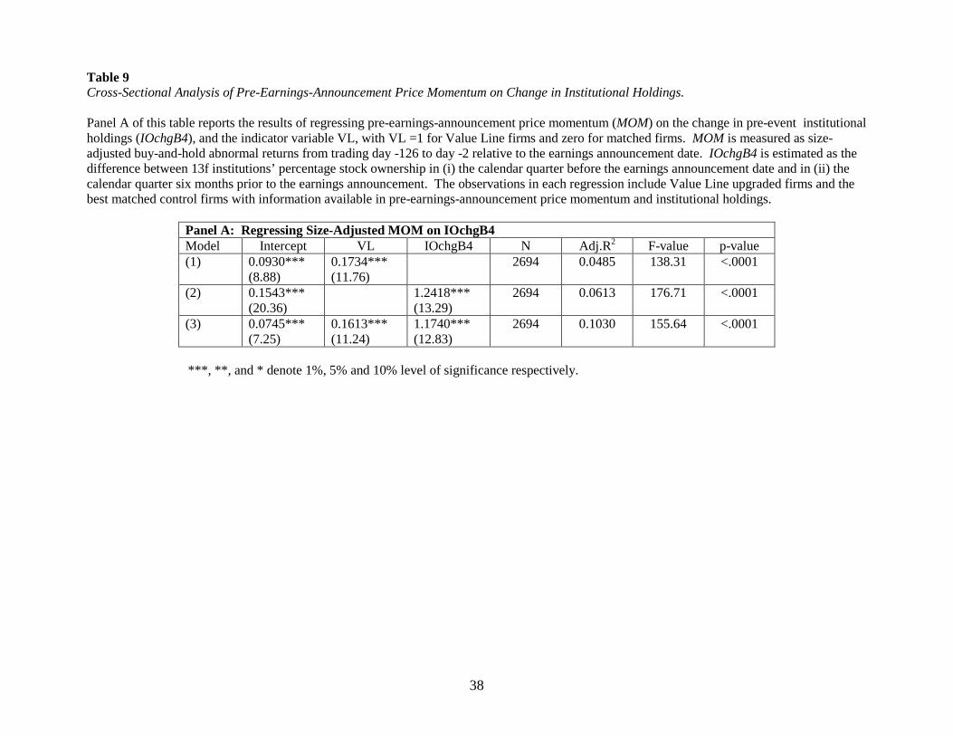
In Table 9, Panel A regression models, the dependent variable is the pre-event

price momentum MOM. In model 1, we find that the Value Line indicator variable is

highly significant (t = 11.76). Clearly, MOM is much higher for our sample Value Line

stocks relative to the matched control firms. We next introduce in model 2, the change in

institutional ownership before the event (IOchgB4); it too is highly significant (t =

13.29). It is not possible for us to determine whether the institutional buy-side pressure is

responsible for the pre-event stock price run-up; or if the institutions notice the price run-

up and purchase the stock. Regardless, we find that there is a strong positive association

between the pre-event price run-up and the change in institutional ownership IOchgB4

over that period.

In Table 9, Panel B, we perform our robustness checks by examining the results in

Panel A with match-adjusted variables. The match-adjusted IOchgB4 remains highly

significant. Institutional investors increase their holdings of the sample firms even before

the Value Line upgrades are announced. We conclude that the change in institutional

20

ownership is a significant factor associated with MOM, the pre-event price momentum

variable.

IV. Conclusions:

Value Line’s timeliness rank upgrades, of the stocks that it covers, have been associated

with a puzzling drift in the post-event period. The issue has been examined by several

financial economists over the past three decades. Prior literature has claimed that the

post-event drift is merely a manifestation of the well-documented post-earnings

announcement drift. Our results demonstrate that Value Line is not merely piggy-backing

on the drift following a publicly disclosed earnings report.

Black (1973) clearly enunciates that price momentum is used by Value Line to

rank stocks but prior research has not used it to unravel the Value Line puzzle. Our

findings corroborate Black’s statement. We find that the pre-event price momentum is a

significant key to the Value Line drift puzzle. Our results suggest that Value Line

upgrades the timeliness ranks of the stocks it covers following large pre-earnings stock

price momentum.

Interestingly, Jegadeesh and Titman (1993) find that the price-momentum effects

are found for periods of less than 12 months. It may be a coincidence that the Value Line

timeliness ranks predict a stock’s performance also for a period of similar length. The

change in institutional ownership before the event is significantly associated with the pre-

event price momentum. The institutional owners seem to recognize the possibility of a

price momentum, or just as likely their buying efforts cause the pre-event price run-up.

Either Value Line is keeping track of institutional ownership or the price momentum of

the stocks that it follows, or both; but it does not necessarily wait for a positive earnings

surprise to upgrade the timeliness of the stocks it covers. Regardless, the pre-event price

momentum is an important explanatory variable for the post-upgrade drift of the Value

Line stocks.17

17 These results must be stated with a caveat: Our findings are based upon a slice of the rank change data. It is not likely but possible, that the results may not hold across all rank upgrades.

21

In conclusion we reiterate that, to its credit, Value Line recognized the momentum

trading rule and has been exploiting the price momentum effect for decades.

22

References:

Affleck-Graves, John, and Richard Mendenhall, 1992, The relation between the Value Line enigma and post-earnings-announcement drift, Journal of Financial Economics 31, 75-96. Ball, Ray and Philip Brown, 1968, An empirical evaluation of accounting income numbers, Journal of Accounting Research 6, 159-178. Barber, Brad, and John Lyon, 1997, Detecting long-run abnormal stock returns: The empirical power and specification of test statistics, Journal of Financial Economics 43, 341-372. Bernard, Victor and Jacob Thomas, 1989, Post-earnings announcement drift: delayed price response or risk premium? , Journal of Accounting Research (Suppl.) 27, 1-36. Black, Fischer, 1973, Yes, Virginia, there is hope: Tests of the Value Line ranking system, Financial Analysts Journal 29 (September), 10-14. Blume, Marshall, and Robert Stambaugh, 1983, Biases in computed returns: An application of the size effect, Journal of Financial Economics 12, 387-404. Copeland, Thomas and David Mayers, 1982, The Value Line enigma (1965-1978): A case study of performance evaluation issues, Journal of Financial Economics 10, 289-322. Fama, Eugene, and Kenneth French, 2006, Dissecting anomalies, CRSP working paper #610. Gregory, N.A., 1983, Testing an aggressive investment strategy using Value Line ranks: A comment, Journal of Finance 38, 257. Hanna, Mark, 1983, Testing an aggressive investment strategy using Value Line ranks: A comment, Journal of Finance 38, 259-262. Holloway, Clark, 1981, A note on testing an aggressive investment strategy using Value Line ranks, Journal of Finance 36, 711-719. Holloway, Clark, 1983, Testing an aggressive investment strategy using Value Line ranks: A reply, Journal of Finance 38, 263-270. Huberman, Gur and Shmuel Kandel, 1987, Value Line rank and size, Journal of Business 60, 577-589. Jegadeesh, Narasimhan and Sheridan Titman, 1993, Returns to buying winners and selling losers: implications for stock market efficiency, Journal of Finance 48, 65-91. Jegadeesh, Narasimhan and Joshua Livnat, 2006, Revenue surprises and stock returns, Journal of Accounting and Economics 41, 147-171. Kaplan, Robert S. and Roman L. Weil, 1973, Risk and the Value Line contest, Financial Analyst Journal 29 (July), 56-60. Kaplan, Robert S. and Roman L. Weil, 1973, Rejoinder to Fisher Black, Financial Analyst Journal 29 (September), p. 14.

23

Peterson, David, 1995, The informative role of the Value Line Investment Survey: Evidence from stock highlights, Journal of Financial and Quantitative Analysis 30, 607-18. Ritter, Jay, 1991, The long-run performance of initial public offerings, Journal of Finance 46, 3-27. Stickel, Scott, 1985, The effect of Value Line Investment Survey rank changes on common stock prices, Journal of Financial Economics 14, 121-143.

24

Table 1 Chronological distribution of Value Line timeliness rank upgrades which ultimately result in a rank of 1.

Year Number of upgrades following an

earnings announcement 1984 12 1985 81 1986 81 1987 92 1988 81 1989 91 1990 97 1991 77 1992 99 1993 92 1994 94 1995 69 1996 78 1997 82 1998 84 1999 89 2000 59 Total 1358

25

Table 2 Industrial sector distribution of Value Line timeliness rank upgrades which ultimately result in a rank of 1. Industrial sectors are determined using I/B/E/S classifications.

Industry Number of upgrades Basic Industries 114 Capital Goods 143 Consumer Durables 77 Consumer Non-durables 138 Consumer Services 269 Energy 30 Finance 115 Health Care 140 Public Utilities 23 Technology 263 Transportation 46 Total 1358

26

Table 3 Sample Characteristics. Matched control firms are obtained from the same industrial sector (determined by I/B/E/S classifications) as the Value Line upgraded firms. The earnings surprise variable is defined as the actual earnings (as reported in the I/B/E/S historical data files) minus the median consensus forecast (from I/B/E/S) immediately preceding the earnings announcement, and then scaled by the stock price (as reported by I/B/E/S) as of the consensus forecast date from the I/B/E/S ancillaries file. The market value of equity is based on the stock price and number of shares outstanding from the I/B/E/S ancillaries file and pertain to their values as of the consensus forecast date immediately preceding the earnings announcement.

Row Item N Mean Median Standard Deviation

Minimum Maximum

1 Earnings surprise for Value Line upgraded firms 1358 0.0026 0.0013 0.0060 -0.0463 0.1033 2 Earnings surprise for the best matched control firm 1358 0.0026 0.0012 0.0059 -0.0403 0.1021

3 Market value of equity for Value Line upgraded firms

1358 3679.81 972.93 12285.11 26.88 224427.59

4 Market value of equity for the best matched control firm

1358 2441.82 420.44 15003.47 4.29 484560.28

5 Number of days from the earnings announcement date to the Value Line upgrade date

1358 15.9278 10 11.0022 2 a 45 b

6

Number of days from the Value Line upgraded firm’s earnings announcement date to the matched control firm’s earnings announcement date (calendar days)

1358 -0.5184 0 8.6026 -15 15

a in trading days. b in calendar days.

27

Table 4 Cross-Sectional Analysis of Post-Earnings-Announcement Drift on Earnings Surprise. Panel A of this table reports the results of analyzing post-earnings-announcement drift (PEAD) on the level of earnings surprise (ESURP), and log value of market capitalization (lnMVE). PEAD is measured as size-adjusted buy-and-hold abnormal returns from trading day 2 through day 120 relative to the earnings announcement date. Level of earnings surprise (ESURP) is obtained at the earnings announcement and measured as the difference between actual earnings and median consensus analyst forecasts, scaled by stock price from I/B/E/S. lnMVE is the natural log of market value of equity in millions as of the statistical period date from I/B/E/S immediately preceding the earnings announcement date. The observations include 1358 Value Line upgraded firms.

Panel A: Regressing PEAD on ESURP and lnMVE in Value Line Upgraded Firms Model Intercept ESURP lnMVE N Adj.R2 F-value p-value (1) 0.0421***

(5.19) 4.5215*** (3.63)

1358 0.0089 13.16 0.0003

(2) 0.1250*** (3.30)

3.9806*** (3.14)

-0.0117** (-2.24)

1358 0.0118 9.10 0.0001

***, **, and * denote 1%, 5% and 10% level of significance respectively.

28

Table 4 (continued) Cross-Sectional Analysis of Post-Earnings-Announcement Drift on Earnings Surprise and Pre-Earnings-Announcement Price Momentum. Panel B of this table reports the results of regressing post-earnings-announcement drift (PEAD) on the level of earnings surprise (ESURP), pre-earnings-announcement price momentum (MOM), log value of market capitalization (lnMVE), and the indicator variable VL, with VL =1 for Value Line firms and zero for matched firms. PEAD is measured as size-adjusted buy-and-hold abnormal returns from trading day 2 through day 120 relative to the announcement date. ESURP is obtained at the earnings announcement and measured as the difference between actual earnings and median consensus analyst forecasts, scaled by stock price. MOM is measured as size-adjusted buy-and-hold abnormal returns from trading day -126 to day -2 relative to the announcement date. lnMVE, is the natural log of market value of equity in millions as of the statistical period date from I/B/E/S, immediately preceding the earnings announcement date. The observations in each regression include 1358 Value Line upgraded firms and the 1358 best matched control firms.

Panel B: Regressing Size-Adjusted PEAD on ESURP and Momentum Model Intercept VL ESURP MOM lnMVE N Adj.R2 F-value p-value (1) 0.0213***

(2.82) 0.0321*** (3.01)

2716 0.0030 9.05 0.0027

(2) 0.0313*** (5.35)

2.3490*** (2.61)

2716 0.0021 6.79 0.0092

(3) 0.0153* (1.93)

0.0320*** (3.00)

2.3406*** (2.60)

2716 0.0051 7.92 0.0004

(4) 0.0113 (1.42)

0.0241** (2.49)

2.2390** (2.49)

0.0457*** (3.28)

2716 0.0086 8.88 <.0001

(5) 0.0584** (2.51)

0.0304*** (2.69)

1.8620** (2.03)

0.0459*** (3.29)

-0.0075** (-2.16)

2716 0.0100 7.83 <.0001


29

Table 4 (continued) Cross-Sectional Analysis of Post-Earnings-Announcement Drift on Earnings Surprise and Pre-Earnings-Announcement Price Momentum. Panel C of this table reports the results of regressing match-adjusted post-earnings-announcement drift (PEAD_MA) on the level of match-adjusted earnings surprises (ESURP_MA), match-adjusted pre-earnings-announcement price momentum (MOM_MA), and match-adjusted log value of market capitalization (lnMVE_MA). PEAD_MA is measured as buy-and-hold returns of Value Line upgraded firms minus buy-and-hold returns of the matched firms from trading day 2 through day 120 relative to the earnings announcement date. ESURP_MA is obtained at the earnings announcement and measured as the difference between actual earnings and median consensus analyst forecasts, scaled by stock price of Value Line upgraded firms minus that of the matched firms. MOM_MA is measured as buy-and-hold returns of Value Line upgraded firms minus that of the matched firms from trading day -126 to day -2 relative to the earnings announcement date. lnMVE_MA is log value of market capitalization in millions of Value Line upgraded firms minus that of the matched firm, where each market value is as of the statistical period date from I/B/E/S immediately preceding the earnings announcement date. The observations in each regression include 1358 Value Line upgraded firms.

Panel C: Regressing Match-Adjusted PEAD on Match-Adjusted ESURP and Match-Adjusted Mom Model Intercept ESURP

_MA MOM _MA

lnMVE _MA

N Adj.R2 F-value p-value

(1) 0.0361*** (3.63)

8.7414 (0.70)

1358 -0.0004 0.50 0.4815

(2) 0.0250** (2.37)

0.0636*** (3.22)

1358 0.0068 10.34 0.0013

(3) 0.0246** (2.33)

9.3165 (0.75)

0.0638*** (3.23)

1358 0.0065 5.45 0.0044

(4) 0.0194* (1.69)

10.0181 (0.81)

0.0641*** (3.24)

0.0060 (1.13)

1358 0.0067 4.06 0.0069


30

Table 5: Calendar time portfolio returns to examine post earnings announcement drift Calendar time portfolios are formed using monthly returns in the period (+1, +6) where month 0 is the month of the earnings announcement. Two types of calendar time portfolios are formed. The first assumes equal weighting while the second assumes value weighting. Both three and four factor models are estimated as shown below:

Fama- French three factor model: tttt,ft,mt,ft,p ehHMLsSMB)rr(rr +++−+=− βα

Fama-French model with momentum factor: ttttt,ft,mt,ft,p epPRIORhHMLsSMB)rr(rr ++++−+=− βα

where rp is the portfolio return from the sample firms, r f is the risk-free rate, rm is the market portfolio return, SMB is the small-firm portfolio return minus the big-firm portfolio return, HML is the high book-to-market portfolio return minus the low book-to-market portfolio return for the three factor model. For the four-factor model, to the three-factors discussed above, we add PRIOR which is the winner portfolio return minus the loser portfolio return based on the past 12-month return. The regression estimate of the intercept term represents the abnormal return for the portfolio after controlling for the Fama-French and momentum factors. The Fama-French SMB and HML factors and the momentum factor, PRIOR, are obtained for similar periods from Kenneth French’s website. The symbols *, **, and *** denote statistical significance at the 10%, 5%, and 1% levels, respectively. Panel A. Event-months (+1, +6) relative to the earnings announcement date (EAD) for the sample of Value Line upgraded stocks

Regression coefficients (ordinary least squares based t-statistic), [heteroskedasticity consistent t-statistic] Row Model

Intercept (rm,t – r f,t) SMB HML PRIOR

Adj.R2

1 Equally weighted portfolio, 3 factor model

0.0070 (3.93)*** [4.39]***

1.1583 (25.00)*** [25.96]***

0.3865 (6.78)*** [6.16]***

0.0502 (0.72) [0.58]

- 0.8369


0.0059 (3.23)*** [3.46]***

1.1589 (25.38)*** [27.09]***

0.3734 (6.62)*** [6.45]***

0.0726 (1.05) [0.91]

0.1084 (2.61)*** [2.24]**

0.8425

3 Value weighted portfolio, 3 factor model

0.0067 (2.83)*** [2.97]***

1.0718 (17.48)*** [19.16]***

-0.0350 (-0.46) [-0.44]

-0.5821 (-6.31)*** [-5.48]***

- 0.7811


0.0046 (1.95)*

[ 1.96]**

1.0729 (18.03)*** [20.48]***

-0.0585 -0.80 -0.76

-0.5421 (-6.01)*** [-5.00]***

0.1940 (3.59)*** [ 2.70]***

0.7948

31

Table 5 (Continued): Calendar time portfolio returns to examine post earnings announcement drift Panel B. Event-months (+1, +6) relative to the Earnings Announcement Date (EAD) for the earnings surprise matched control firm stocks



Adj.R2


0.0022 (1.29) [1.42]

1.1863 (26.93)*** [25.08]***

0.5447 (10.05)*** [6.03]***

0.0253 (0.38) [0.36]

- 0.8679


0.0028 (1.58) [1.55]

1.1861 (26.98)*** [25.24]***

0.5513 (10.15)*** [6.27]***

0.0141 (0.21) [0.19]

-0.0543 (-1.36) [-0.85]

0.8692


0.0025 (0.94) [0.91]

1.0411 (14.97)*** [15.35]***

0.0944 (1.10) [0.65]

-0.3409 (-3.26)*** [-2.46]**

- 0.6934


0.0033 (1.18) [1.01]

1.0407 (14.98)*** [15.25]***

0.1028 (1.20) [0.69]

-0.3553 (-3.37)*** [-2.61]***

-0.0697 -1.11 -0.49

0.6953

32

Table 6 Cross-Sectional Analysis of Post-Upgrade Drift on Earnings Surprise and Pre-Earnings-Announcement Price Momentum. This table reports the results of analyzing post-upgrade drift (PUD) on the level of earnings surprise (ESURP), pre-earnings-announcement price momentum (MOM), and log value of market capitalization (lnMVE). PUD is measured as size-adjusted buy-and-hold abnormal returns from trading day 2 through day 120 relative to Value Line upgrade date. ESURP is obtained at the earnings announcement and measured as the difference between actual earnings and median consensus analyst forecasts, scaled by stock price from I/B/E/S. MOM is measured as size-adjusted buy-and-hold abnormal returns from trading day -126 to day -2 relative to the earnings announcement. lnMVE is the natural log of market value of equity in millions as of the statistical period date from I/B/E/S immediately preceding the earnings announcement date. The observations include 1358 Value Line upgraded firms.

Regressing PUD on ESURP and MOM in Value Line Upgraded Firms Model Intercept ESURP MOM lnMVE N Adj.R2 F-value p-value (1) 0.0182**

(2.26) 2.0675* (1.67)

1358 0.0013 2.77 0.0961

(2) 0.0018 (0.20)

0.0821*** (4.41)

1358 0.0134 19.45 <.0001

(3) -0.0032 (-0.34)

1.9587 (1.59)

0.0815*** (4.38)

1358 0.0145 11.00 <.0001

(4) -0.0405 (-1.07)

2.2024* (1.75)

0.0815*** (4.38)

0.0053 (1.02)

1358 0.0145 7.68 <.0001


33

Table 7 Cross-Sectional Analysis of Post-Upgrade Drift on Earnings Surprise and Pre-Earnings Announcement Price Momentum. Panel A of this table reports the results of regressing post-upgrade drift (PUD) on the level of earnings surprise (ESURP), pre-earnings announcement price momentum (MOM), log value of market capitalization (lnMVE), and the indicator variable VL, with VL =1 for Value Line firms and zero for matched firms. PUD of Value Line upgraded firms is measured as size-adjusted buy-and-hold abnormal returns from trading day 2 through day 120 relative to Value Line upgrade date. PUD of the best matched control firms is measured as size-adjusted buy-and-hold abnormal returns from day 2 through day 120 relative to pseudo Value Line upgrade date. Pseudo Value Line upgrade date is obtained so that the number of trading days between the best matched firm’s earnings announcement and its pseudo Value Line upgrade date is the same as the number of trading days between Value Line upgraded firm’s earnings announcement and its Value Line upgrade date. ESURP is obtained at the earnings announcement and measured as the difference between actual earnings and median consensus analyst forecasts, scaled by stock price. MOM is measured as size-adjusted buy-and-hold abnormal returns from trading day -126 to day -2 relative to the earnings announcement date. lnMVE, is the natural log of market value of equity in millions as of the statistical period date from I/B/E/S, immediately preceding the earnings announcement date. The observations in each regression include 1358 Value Line upgraded firms and the 1358 best matched control firms.

Panel A: Regressing Size-Adjusted PUD on ESURP and MOM Model Intercept VL ESURP MOM lnMVE N Adj.R2 F-value p-value (1) 0.0208***

(2.74) 0.0028 (0.26)

2716 -0.0003 0.07 0.7953

(2) 0.0174** (2.18)

0.0027 (0.25)

1.3314 (1.47)

2716 0.0001 1.11 0.3291

(3) 0.0137* (1.79)

-0.0107 (-0.97)

0.0773*** (5.53)

2716 0.0104 15.31 <.0001

(4) 0.0107 (1.34)

-0.0106 (-0.97)

1.1609 (1.29)

0.0767*** (5.48)

2716 0.0107 10.76 <.0001

(5) 0.0142 (0.61)

-0.0102 (-0.89)

1.1332 (1.23)

0.0767*** (5.48)

-0.0006 (-0.16)

2716 0.0103 8.08 <.0001


34

Table 7 (continued) Cross-Sectional Analysis of Post-Upgrade Drift on Earnings Surprise and Pre-Earnings-Announcement Price Momentum. Panel B of this table reports the results of regressing match-adjusted post-upgrade drift (PUD_MA) on the level of match-adjusted earnings surprises (ESURP_MA), match-adjusted pre-announcement momentum (MOM_MA), and match-adjusted log value of market capitalization (lnMVE_MA). PUD_MA is measured as buy-and-hold returns of Value Line upgraded firms minus buy-and-hold returns of the matched firms from trading day 2 through day 120 relative to Value Line or pseudo Value Line upgrade date. ESURP_MA is obtained at the earnings announcement and measured as the difference between the actual earnings and median consensus analyst forecasts, scaled by stock price of Value Line upgraded firms minus that of the matched firms. MOM_MA is measured as buy-and-hold returns of Value Line upgraded firms minus that of the matched firms from trading day -126 to day -2 relative to the earnings announcement date. lnMVE_MA is log value of market capitalization in millions of Value Line upgraded firms minus that of the matched firm, where each market value is as of the statistical period date from I/B/E/S immediately preceding the earnings announcement date. The observations in each regression include 1358 Value Line upgraded firms.

Panel B: Regressing Match-Adjusted PUD on Match-Adjusted ESURP and Match-Adjusted MOM Model Intercept ESURP

_MA MOM _MA

lnMVE _MA

N Adj.R2 F-value p-value

(1) 0.0086 (0.74)

-2.5111 (-0.17)

1358 -0.0007 0.03 0.8628

(2) -0.0168 (-1.38)

0.1404*** (6.13)

1358 0.0262 37.54 <.0001

(3) -0.0168 (-1.37)

-1.2463 (-0.09)

0.1404*** (6.12)

1358 0.0255 18.76 <.0001

(4) -0.0282** (-2.12)

0.3153 (0.02)

0.1410*** (6.16)

0.0134** (2.18)

1358 0.0282 14.12 <.0001


35

Table 7 (continued) Cross-Sectional Analysis of Post-Upgrade Drift on Earnings Surprise and Pre-Earnings-Announcement Price Momentum. Panel C of this table reports the results of analyzing post-upgrade drift (PUD) of the best matched control firms, on the level of earnings surprise (ESURP), pre-earnings-announcement price momentum (MOM), and log value of market capitalization (lnMVE). PUD is measured as size-adjusted buy-and-hold abnormal returns from day 2 through day 120 relative to pseudo Value Line upgrade date. Pseudo Value Line upgrade date is obtained so that the number of trading days between the best matched firm’s earnings announcement and its pseudo Value Line upgrade date is the same as the number of trading days between Value Line upgraded firm’s earnings announcement and its Value Line upgrade date. ESURP is obtained at the earnings announcement and measured as the difference between actual earnings and median consensus analyst forecasts, scaled by stock price from I/B/E/S. MOM is measured as size-adjusted buy-and-hold abnormal returns from trading day -126 to day -2 relative to the earnings announcement. lnMVE is the natural log of market value of equity in millions as of the statistical period date from I/B/E/S immediately preceding the earnings announcement date. The observations include the 1358 best matched control firms.

Panel C: Regressing PUD on ESURP and MOM in the Best Matched Control Firms Model Intercept ESURP MOM lnMVE N Adj.R2 F-value p-value (1) 0.0197**

(2.29) 0.5669 (0.43)

1358 -0.0006 0.18 0.6707

(2) 0.0144* (1.78)

0.0736*** (3.47)

1358 0.0081 12.05 0.0005

(3) 0.0135 (1.55)

0.3375 (0.25)

0.0733*** (3.45)

1358 0.0074 6.05 0.0024

(4) 0.0449 (1.43)

0.0664 (0.05)

0.0736*** (3.47)

-0.0050 (-1.04)

1358 0.0075 4.40 0.0044


36

Table 8: Calendar time portfolio returns to examine post upgrade drift Calendar time portfolios are formed using monthly returns in the period (+1, +6) where month 0 is the month of the Value Line date (pseudo Value Line date) for Value Line upgraded stocks (matched control firms). The pseudo Value Line date occurs the same number of trading days after the earnings announcement date for the matched control firm as does the Value Line date after the earnings announcement date for the Value Line upgraded stock. Two types of calendar time portfolios are formed. The first assumes equal weighting while the second assumes value weighting. Both three and four factor models are estimated as shown below:

Fama- French three factor model: tttt,ft,mt,ft,p ehHMLsSMB)rr(rr +++−+=− βα

Fama-French model with momentum factor: ttttt,ft,mt,ft,p epPRIORhHMLsSMB)rr(rr ++++−+=− βα

where rp is the portfolio return from the sample firms, r f is the risk-free rate, rm is the market portfolio return, SMB is the small-firm portfolio return minus the big-firm portfolio return, HML is the high book-to-market portfolio return minus the low book-to-market portfolio return for the three factor model. For the four-factor model, to the three-factors discussed above, we add PRIOR which is the winner portfolio return minus the loser portfolio return based on the past 12-month return. The regression estimate of the intercept term represents the abnormal return for the portfolio after controlling for the Fama-French and momentum factors. The Fama-French SMB and HML factors and the momentum factor, PRIOR, are obtained for similar periods from Kenneth French’s website. The symbols *, **, and *** denote statistical significance at the 10%, 5%, and 1% levels, respectively. Panel A. Event-months (+1, +6) relative to the Value Line date for the sample of Value Line upgraded stocks



Adj.R2


0.0033 (1.80)*

[2.03]**

1.1755 (25.20)*** [27.06]***

0.3293 5.74*** 6.15***

0.0432 0.62 0.53

- 0.8365


0.0025 1.33 1.41

1.1758 (25.35)*** [28.02]***

0.3201 (5.59)*** (5.84)***

0.0585 (0.83) [0.77]

0.0749 (1.78)* [1.66]*

0.8391


0.0053 (2.20)* (2.36)*

1.139 (18.28)*** [19.59]***

-0.0781 (-1.02) [-0.79]

-0.4281 (-4.57)*** [-3.31]***

- 0.7698


0.0031 (1.27) [1.32]

1.1398 (18.97)*** [19.64]***

-0.1045 (-1.41) [-1.06]

-0.3841 (-4.22)*** [-3.16]***

0.2151 (3.94)*** [2.66]***

0.7871

37

Table 8 (Continued): Calendar time portfolio returns to examine post upgrade drift Panel B. Event-months (+1, +6) relative to the pseudo Value Line date for the earnings surprise matched control firm stocks



Adj.R2


0.00 (0.01) [0.01]

1.1113 (17.02)*** [17.04]***

0.5752 (7.15)*** [5.97]***

-0.0003 (0.00) [0.00]

- 0.7369


-0.0005 (-0.18) [-0.15]

1.1122 (17.02)*** [17.48]***

0.5687 (7.03)*** [5.92]***

0.009 (0.09) [0.09]

0.0494 (0.84) [0.39]

0.7379


0.0017 (0.53) [0.55]

0.9242 (11.26)*** [10.46]***

0.1029 (1.02) [0.87]

-0.3526 (-2.86)*** [-2.35]**

- 0.5779


0.0014 (0.42) [0.33]

0.9247 (11.24)*** [10.66]***

0.0988 (0.97) [0.83]

-0.3467 (-2.79)*** [-2.13]**

0.031 (0.42) [0.17]

0.5783

38

Table 9 Cross-Sectional Analysis of Pre-Earnings-Announcement Price Momentum on Change in Institutional Holdings. Panel A of this table reports the results of regressing pre-earnings-announcement price momentum (MOM) on the change in pre-event institutional holdings (IOchgB4), and the indicator variable VL, with VL =1 for Value Line firms and zero for matched firms. MOM is measured as size-adjusted buy-and-hold abnormal returns from trading day -126 to day -2 relative to the earnings announcement date. IOchgB4 is estimated as the difference between 13f institutions’ percentage stock ownership in (i) the calendar quarter before the earnings announcement date and in (ii) the calendar quarter six months prior to the earnings announcement. The observations in each regression include Value Line upgraded firms and the best matched control firms with information available in pre-earnings-announcement price momentum and institutional holdings.

Panel A: Regressing Size-Adjusted MOM on IOchgB4 Model Intercept VL IOchgB4 N Adj.R2 F-value p-value (1) 0.0930***

(8.88) 0.1734*** (11.76)

2694 0.0485 138.31 <.0001

(2) 0.1543*** (20.36)

1.2418*** (13.29)

2694 0.0613 176.71 <.0001

(3) 0.0745*** (7.25)

0.1613*** (11.24)

1.1740*** (12.83)

2694 0.1030 155.64 <.0001


39

Table 9 (continued) Cross-Sectional Analysis of Pre-Earnings-Announcement Price Momentum on Change in Institutional Holdings. Panel B of this table reports the results of regressing match-adjusted pre-earnings-announcement price momentum (MOM_MA) on match-adjusted change in pre-event institutional holdings (IOchgB4_MA). MOM_MA is measured as buy-and-hold returns of Value Line upgraded firms minus that of the matched firms from trading day -126 to day -2 relative to the earnings announcement date. IOchgB4_MA is measured as IOchgB4 of Value Line upgraded firms minus that of the matched firms. The observations in each regression include Value Line upgraded firms with information available in match-adjusted pre-earnings-announcement price momentum and match-adjusted change in institutional holdings.

Panel B: Regressing Match-Adjusted MOM on Match-Adjusted IOchgB4 Model Intercept IOchgB4

_MA N Adj.R2 F-value p-value

(1) 0.1704*** (12.54)

0.8181*** (6.44)

1336 0.0294 41.48 <.0001


40

Figure 1: Timeline illustrating sample selection process A dataset containing all upgrades to a timeliness rank of 1 spanning the time span from 01/01/1984 to 10/06/2000 was obtained from the Value Line Investment Survey. The Value Line dataset contains an item called “Press Date”, the day on which the weekly insert containing the timeliness rank change goes to the printers. The average subscriber receives the publication with the timeliness rank upgrade information on the Friday following the Press Date (see Peterson, 1995). We designate the Friday following the Press Date as the Value Line upgrade date (VLD). Using these dates, the most immediately preceding earnings announcement date, EAD, is identified. All upgrades to a timeliness rank of 1, where the time elapsed between EAD and VLD, is as shown below, are retained for use in our sample.

EAD VLD

STEP 2 The earnings announcement

date, EAD, immediately preceding VLD is identified

STEP 1 First, the Value Line

Date VLD, is identified

STEP 3 Retain only those upgrades to a timeliness rank of 1, where the

minimum time between EAD and VLD is 2 trading days and the

maximum time between the two dates is 45 calendar days.

41

EAD

EAD-1 EAD+1

VLD

VLD-1 VLD+1 EAD-2 VLD-2 EAD+2 VLD+2 EAD-126 VLD+120

26.38% a 1237:121 a

3.52% a 1000:358 a

1.77% a 806:552 a

1.77% a 902:456 a

3.04% a 664:690

Value Line Upgraded Firms 1

Best Matched Control Firms 2

8.11% a 788:570 a

1.47% a 793:565 a

0.34% d 680:678

-0.09% 641:717

1.52% d 647:692

Matched Pair Test Results 3

18.26% a t=13.47a

2.04% a t=8.429 a

1.44% a t=5.73 a

1.69% a t=9.54 a

1.30% t=1.12

Figure 2: Event study results In the figure below, event study results are shown for the sample of Value Line upgraded firms and for the sample of firms matched by earnings surprise. EAD represents the earnings announcement date, while VLD denotes the date on which market participants learned of the upgrade from Value Line. We give each control firm a pseudo upgrade date. Pseudo upgrade date is defined for the control firm such that the number of trading days between the best matched firm’s earnings announcement and its pseudo Value Line upgrade date is the same as the number of trading days between Value Line upgraded firm’s earnings announcement and its Value Line upgrade date. In the event study, size adjusted abnormal returns were computed for both samples. An estimation period of 255 days ending on day EAD-127 was used to assess the proportion of positive to negative returns used in computing non-parametric sign tests. 1, 2 : For each window, the top number represents the mean size adjusted abnormal return, while the bottom row provides the number of positive to negative

size adjusted returns. 3 : For the matched pair test results, the top number is the mean matched pair difference in event window size adjusted returns, and the letter in subscripts

(if any) denotes the level of significance in a two tailed test of a nonparametric Wilcoxon signed rank test statistic. The bottom row provides a t-statistic and the letter (if any) next to the t-value indicates the level of significance in a two tailed test.

a, d : Significant at the .0001 and .1 levels, respectively

Unraveling a puzzle: The case of Value Line timeliness ... · been exploiting the price momentum...

Documents

Transcript of Unraveling a puzzle: The case of Value Line timeliness ... · been exploiting the price momentum...