Tony ArberUniversity of Warwick

STFC Advanced School, MSSL September 2013.

Fundamentals of Magnetohydrodynamics

(MHD)

Aim

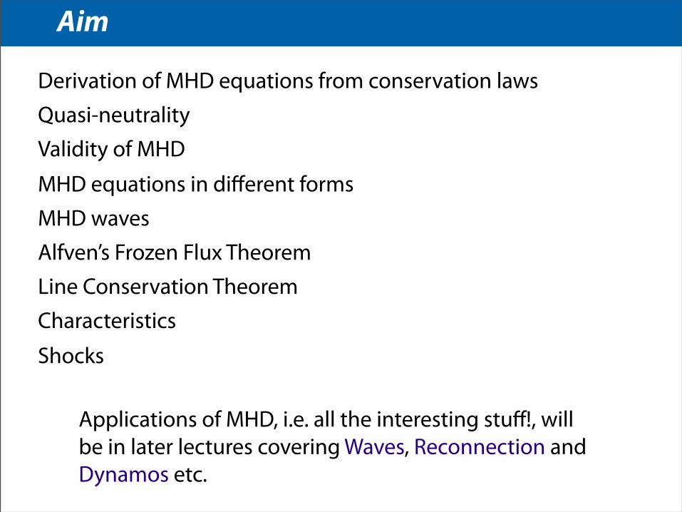
Derivation of MHD equations from conservation lawsQuasi-neutralityValidity of MHDMHD equations in different forms MHD wavesAlfven’s Frozen Flux TheoremLine Conservation TheoremCharacteristicsShocks

Applications of MHD, i.e. all the interesting stuff!, will be in later lectures covering Waves, Reconnection and Dynamos etc.

Derivation of MHD

Possible to derive MHD from

• N-body problem to Klimotovich equation, then take moments and simplify to MHD

• Louiville theorem to BBGKY hierarchy, then take moments and simplify to MHD

• Simple fluid dynamics and control volumes

First two are useful if you want to study kinetic theory along the way but all kinetics removed by the end

Final method followed here so all physics is clear

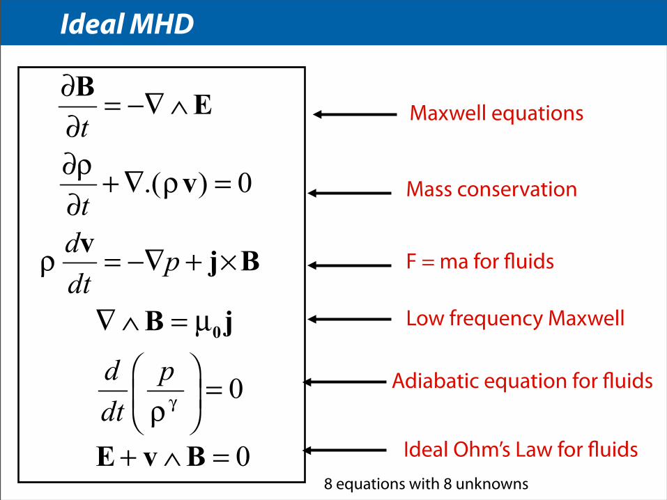
Ideal MHD

8 equations with 8 unknowns

Maxwell equations

Mass conservation

F = ma for fluids

Low frequency Maxwell

Adiabatic equation for fluids

Ideal Ohm’s Law for fluids

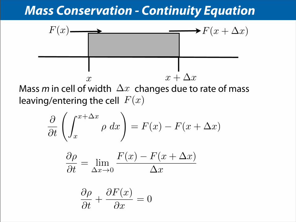
Mass Conservation - Continuity Equation

x

x+�x

m =

Zx+�x

x

⇢ dx

F (x+�x)F (x)

Mass m in cell of width changes due to rate of mass leaving/entering the cell

�x

F (x)

@

@t

Zx+�x

x

⇢ dx

!= F (x)� F (x+�x)

@⇢

@t

= lim�x!0

F (x)� F (x+�x)

�x

@⇢

@t

+@F (x)

@x

= 0

Mass flux - conservation laws@⇢

@t

+@F (x)

@x

= 0

Mass flux per second through cell boundary

In 3D this generalizes to

This is true for any conserved quantity so if conserved

@⇢

@t+r.(⇢v) = 0

F (x, t) = ⇢(x, t) vx

(x, t)

ZU dx

@U

@t+r.F = 0

Hence applies to mass density, momentum density and energy density for example.

Convective Derivative

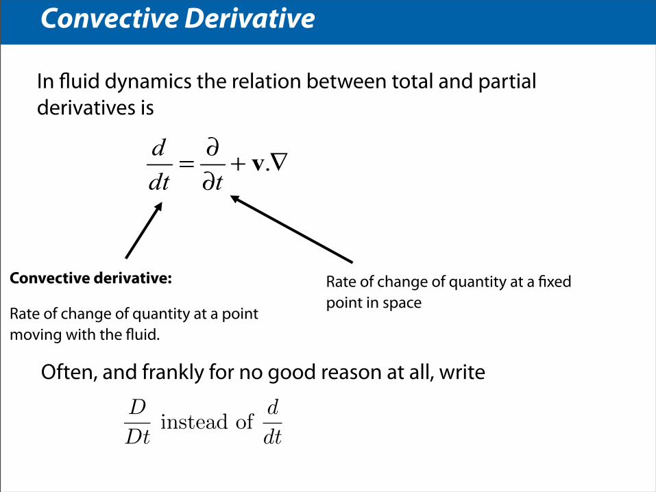
In fluid dynamics the relation between total and partial derivatives is

Rate of change of quantity at a fixed point in space

Convective derivative:

Rate of change of quantity at a point moving with the fluid.

Often, and frankly for no good reason at all, write

D

Dtinstead of

d

dt

Adiabatic energy equation

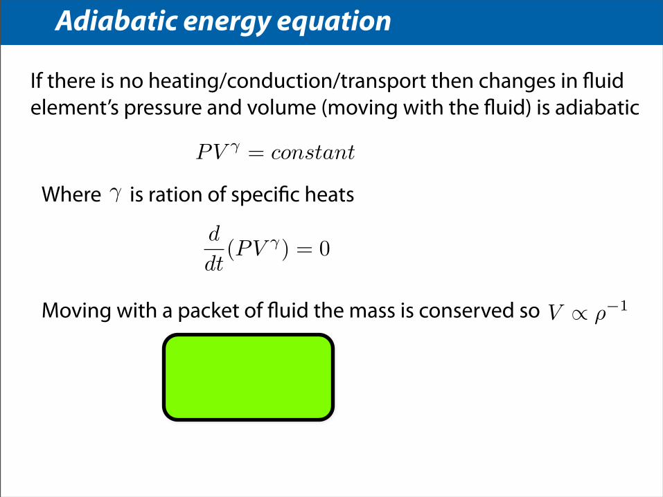
If there is no heating/conduction/transport then changes in fluid element’s pressure and volume (moving with the fluid) is adiabatic

PV

� = constant

d

dt(PV �) = 0

Where is ration of specific heats�

Moving with a packet of fluid the mass is conserved so V / ⇢�1

d

dt

✓P

⇢�

◆= 0

Momentum equation - Euler fluid

x

x+�x

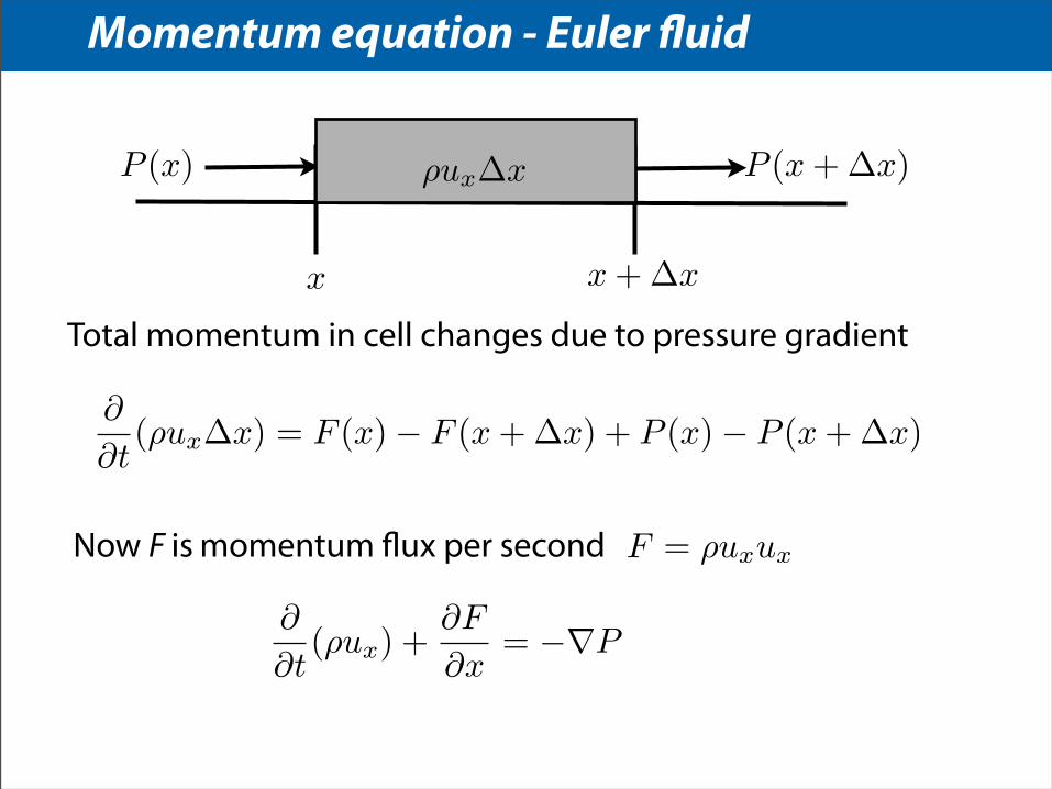
Total momentum in cell changes due to pressure gradient

P (x) P (x+�x)⇢u

x

�x

Now F is momentum flux per second F = ⇢ux

ux

@

@t

(⇢ux

) +@F

@x

= �rP

@

@t

(⇢ux

�x) = F (x)� F (x+�x) + P (x)� P (x+�x)

Momentum equation - Euler fluid

⇢

@u

x

@t

+ ⇢u

x

@u

x

@x

= �rP

Use mass conservation equation to rearrange as

⇢

✓@u

x

@t

+ u

x

@u

x

@x

◆= �rP

⇢du

x

dt= �rP

du

x

(x, t)

dt

=@u

x

@t

+@x

@t

@u

x

@x

Since by chain rule

Momentum equation - MHD

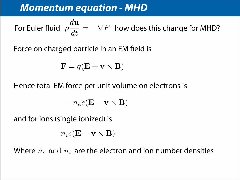
⇢du

dt= �rPFor Euler fluid how does this change for MHD?

Force on charged particle in an EM field is

F = q(E+ v ⇥B)

Hence total EM force per unit volume on electrons is

�nee(E+ v ⇥B)

and for ions (single ionized) is

nie(E+ v ⇥B)

Where are the electron and ion number densitiesne and ni

Momentum equation - MHD

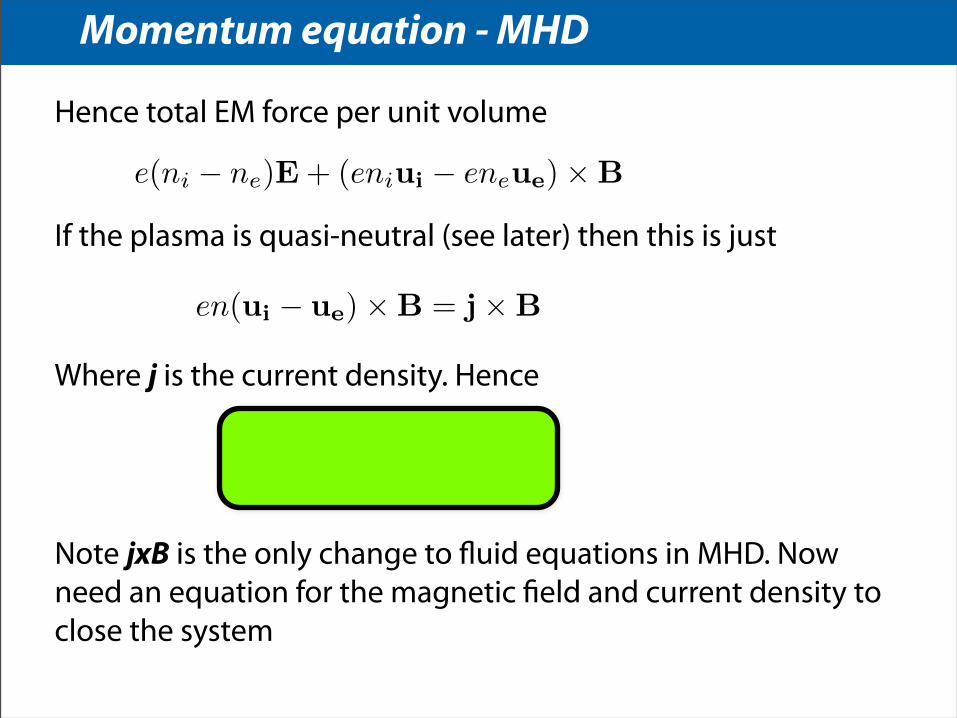
Hence total EM force per unit volume

If the plasma is quasi-neutral (see later) then this is just

en(ui � ue)⇥B = j⇥B

Where j is the current density. Hence

⇢du

dt= �rP + j⇥B

Note jxB is the only change to fluid equations in MHD. Now need an equation for the magnetic field and current density to close the system

e(ni � ne)E+ (eniui � eneue)⇥B

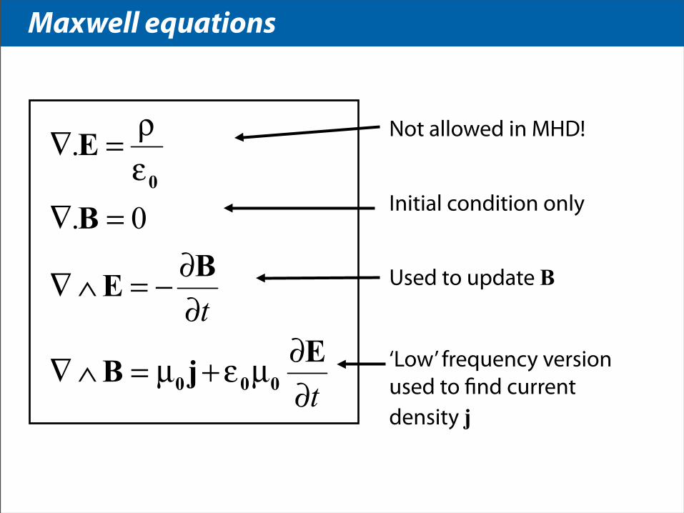
Maxwell equations

Not allowed in MHD!

Initial condition only

Used to update B

‘Low’ frequency version used to find current density j

Low-frequency Maxwell equations

So for low velocities/frequencies we can ignore the displacement current

Displacement current

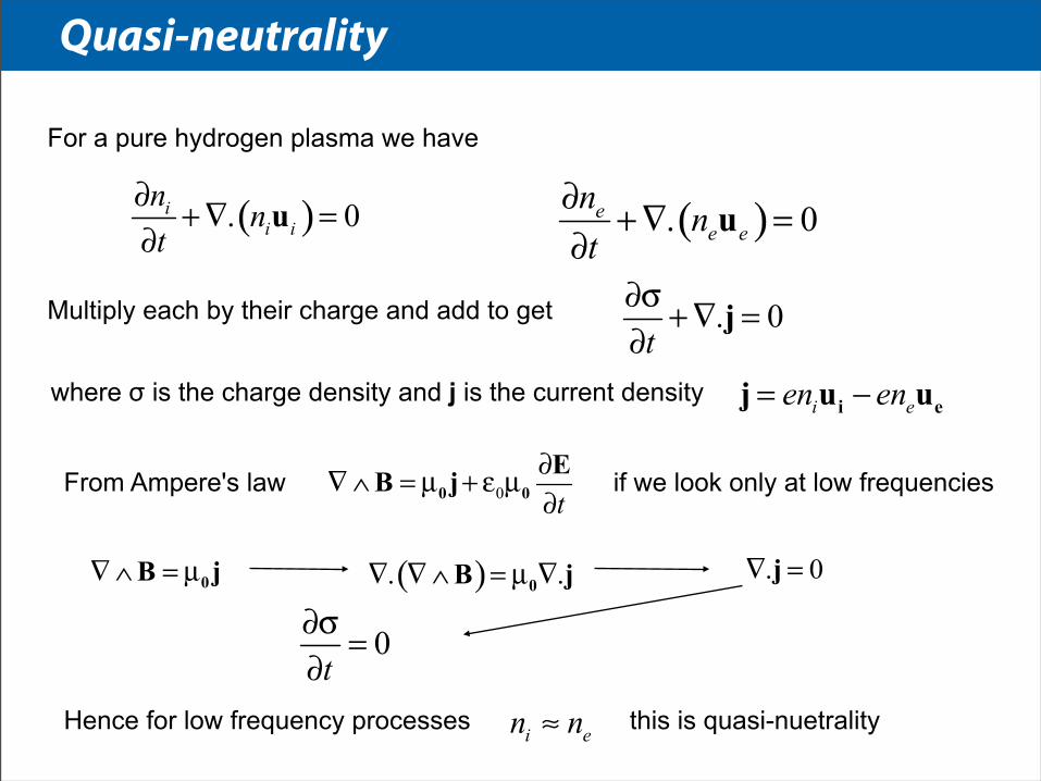
Quasi-neutrality

For a pure hydrogen plasma we have

Multiply each by their charge and add to get

where σ is the charge density and j is the current density

From Ampere's law if we look only at low frequencies

Hence for low frequency processes this is quasi-nuetrality

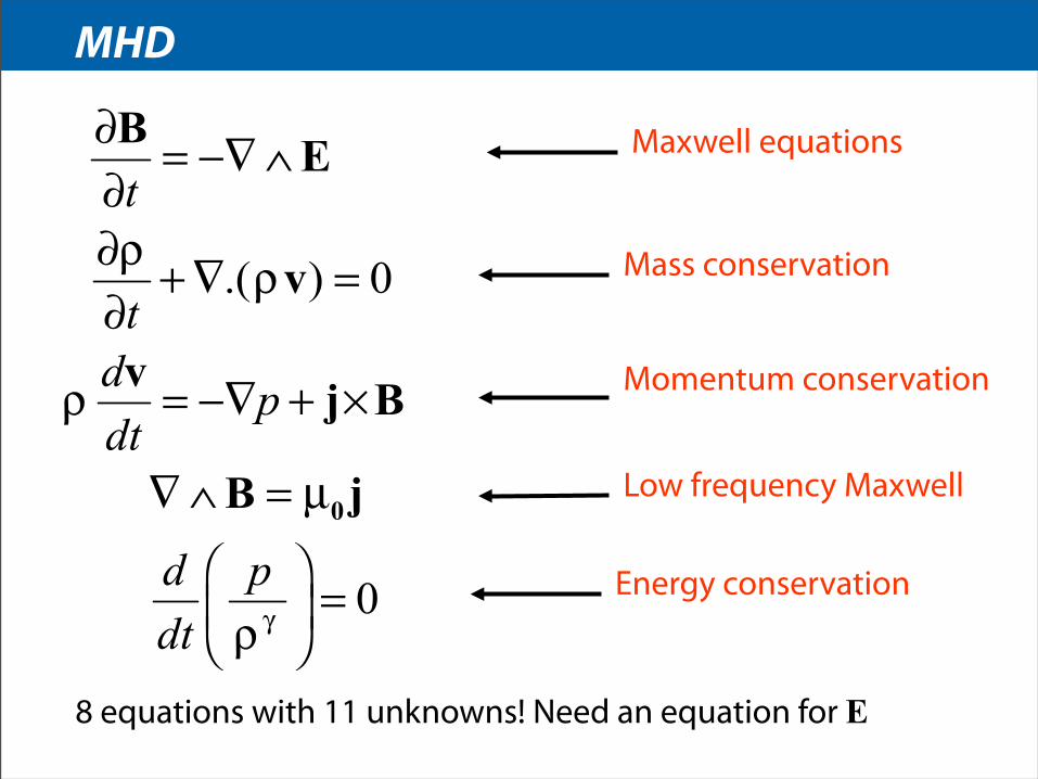
MHD

8 equations with 11 unknowns! Need an equation for E

Maxwell equations

Mass conservation

Momentum conservation

Low frequency Maxwell

Energy conservation

Ohm's Law

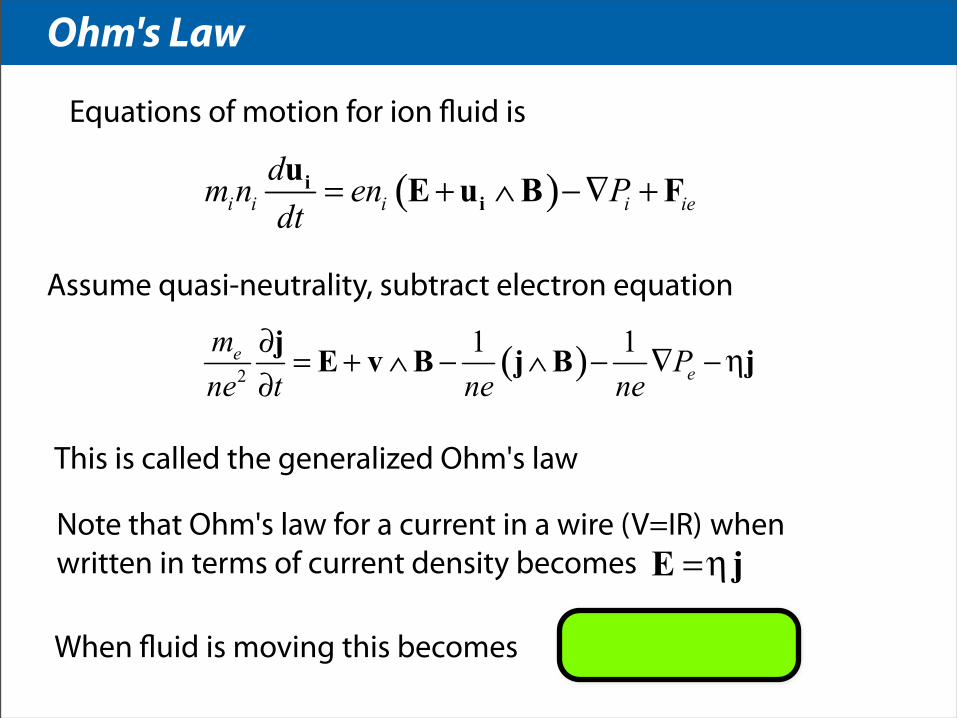
Assume quasi-neutrality, subtract electron equation

Note that Ohm's law for a current in a wire (V=IR) when written in terms of current density becomes

This is called the generalized Ohm's law

When fluid is moving this becomes

Equations of motion for ion fluid is

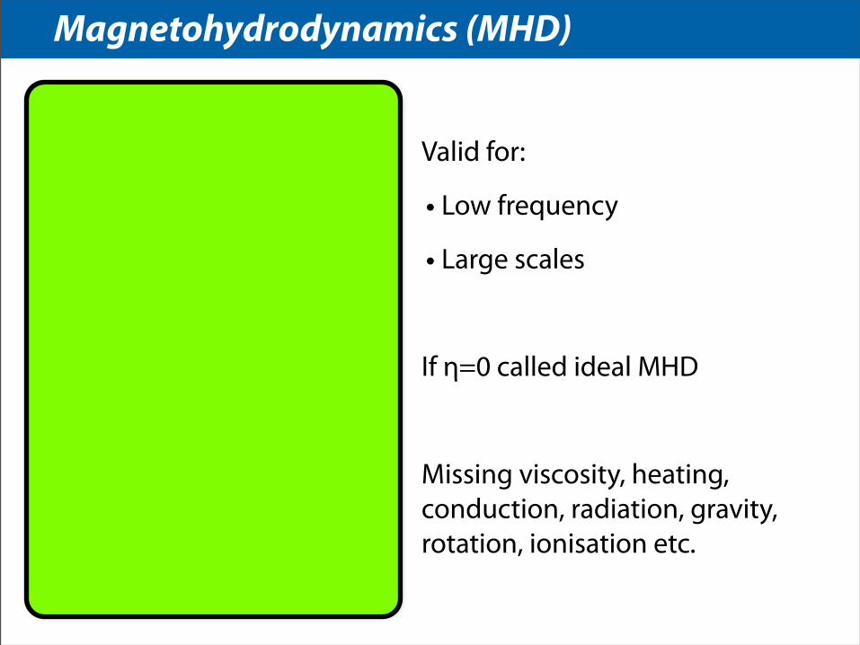
Magnetohydrodynamics (MHD)

Valid for:

• Low frequency

• Large scales

If η=0 called ideal MHD

Missing viscosity, heating, conduction, radiation, gravity, rotation, ionisation etc.

Validity of MHD

Assumed quasi-neutrality therefore must be low frequency and speeds << speed of light

Assumed scalar pressure therefore collisions must be sufficient to ensure the pressure is isotropic. In practice this means:

• mean-free-path << scale-lengths of interest• collision time << time-scales of interest• Larmor radii << scale-lengths of interest

However as MHD is just conservation laws plus low-frequency MHD it tends to be a good first approximation to much of the physics even when all these conditions are not met.

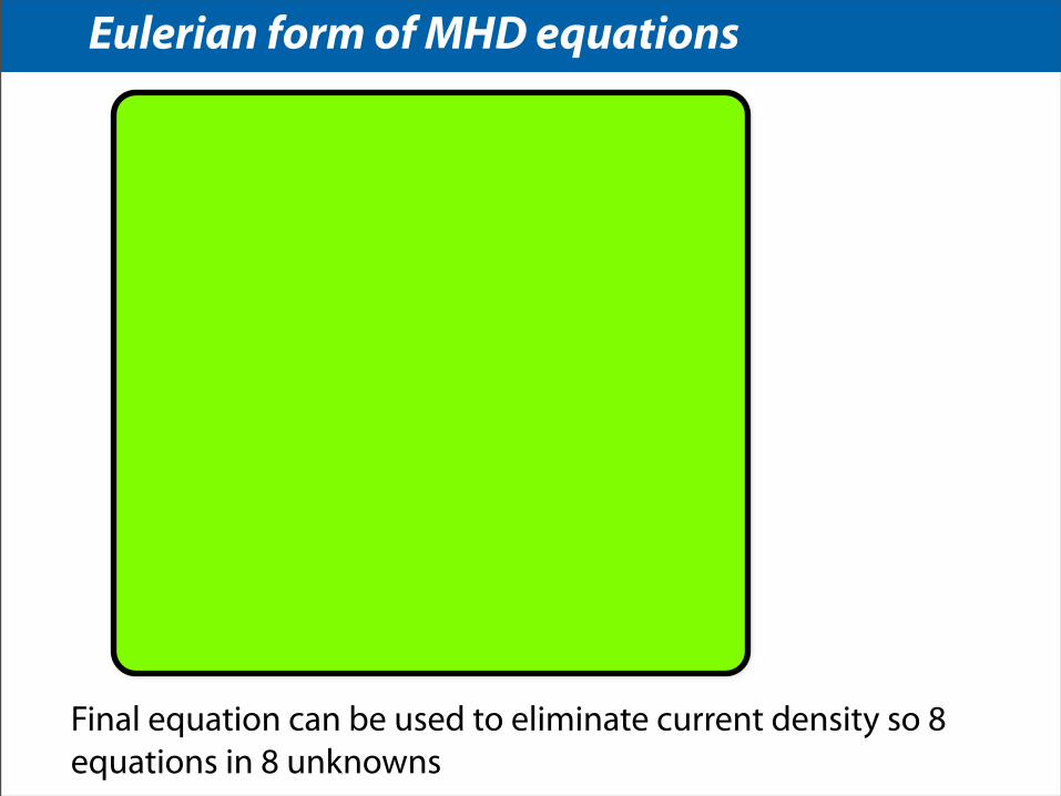
Eulerian form of MHD equations

@⇢

@t= �r.(⇢v)

@P

@t= ��Pr.v

@v

@t= �v.r.(v)� 1

⇢r.P +

1

⇢j⇥B

@B

@t= r⇥ (v ⇥B)

j =1

µ0r⇥B

Final equation can be used to eliminate current density so 8 equations in 8 unknowns

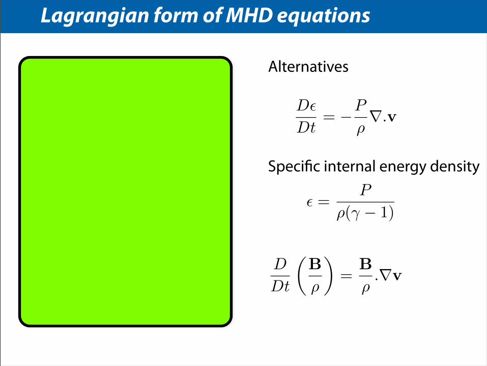
Lagrangian form of MHD equations

j =1

µ0r⇥B

D⇢

Dt= �⇢r.v

DP

Dt= ��Pr.v

Dv

Dt= �1

⇢r.P +

1

⇢j⇥B

DB

Dt= (B.r)v �B(r.v)

D

Dt

✓B

⇢

◆=

B

⇢.rv

✏ =P

⇢(� � 1)

Alternatives

Specific internal energy density

D✏

Dt= �P

⇢r.v

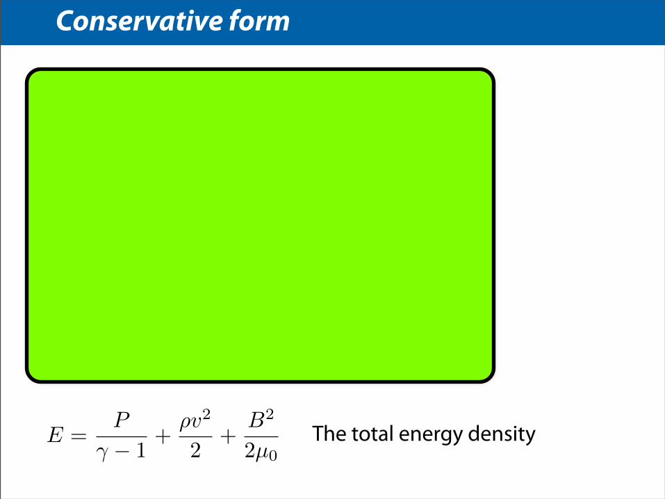
Conservative form

@⇢

@t= �r.(⇢v)

@⇢v

@t= �r.

✓⇢vv + I(P +

B2

2)�BB

◆

@E

@t= �r.

✓✓E + P +

B2

2µ0

◆v �B(v.B)

◆

@B

@t= �r(vB�Bv)

E =P

� � 1+

⇢v2

2+

B2

2µ0The total energy density

Plasma beta

A key dimensionless parameter for ideal MHD is the plasma-beta

It is the ratio of thermal to magnetic pressure

� =2µ0P

B2

Low beta means dynamics dominated by magnetic field, high beta means standard Euler dynamics more important

� / c2sv2A

Assume initially in stationary equilibrium

MHD Waves

r.P0 = j0 ⇥B0

Apply perturbation, e.g. P = P0 + P1

Simplify to easiest case with constant and no equilibrium current or velocity

⇢0, P0,B0 = B0z

Univorm B field

Constant density, pressureZero initial velocityApply small perturbation to system

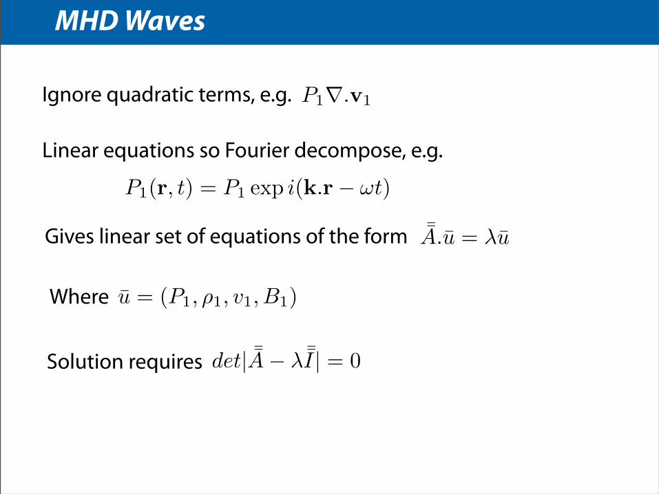
MHD Waves

Ignore quadratic terms, e.g. P1r.v1

Linear equations so Fourier decompose, e.g.

P1(r, t) = P1 exp i(k.r� !t)

Gives linear set of equations of the form ¯A.u = �u

Where u = (P1, ⇢1, v1, B1)

Solution requires det| ¯A� � ¯I| = 0

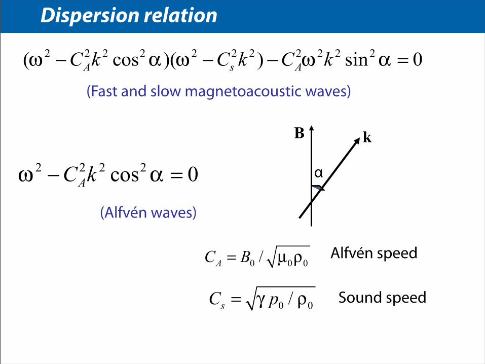
(Fast and slow magnetoacoustic waves)

(Alfvén waves)

Alfvén speed

Sound speed

B k

α

Dispersion relation

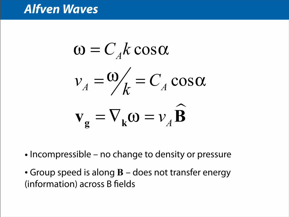
• Incompressible – no change to density or pressure

• Group speed is along B – does not transfer energy (information) across B fields

Alfven Waves

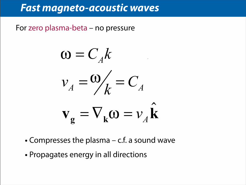
For zero plasma-beta – no pressure

• Compresses the plasma – c.f. a sound wave

• Propagates energy in all directions

Fast magneto-acoustic waves

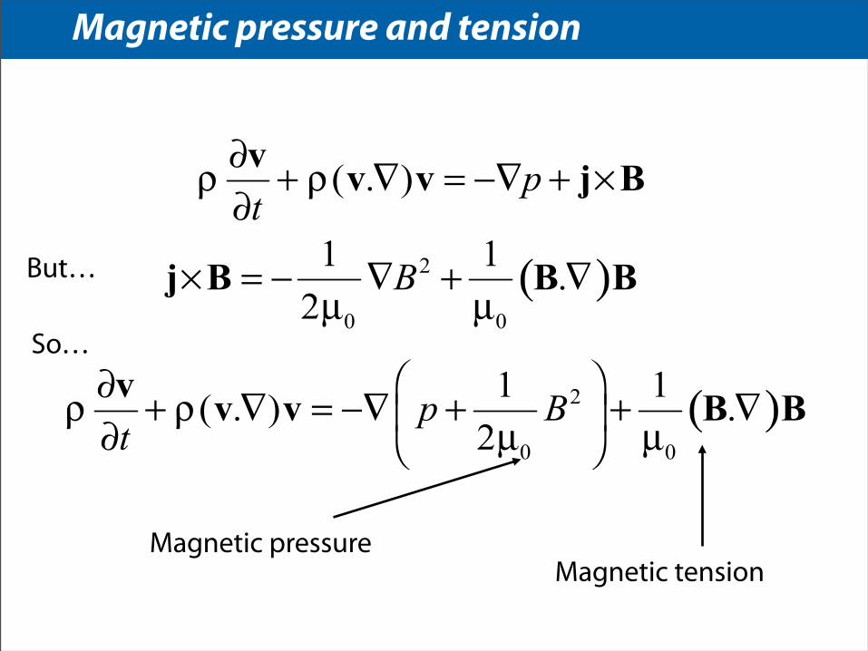
But…

So…

Magnetic pressureMagnetic tension

Magnetic pressure and tension

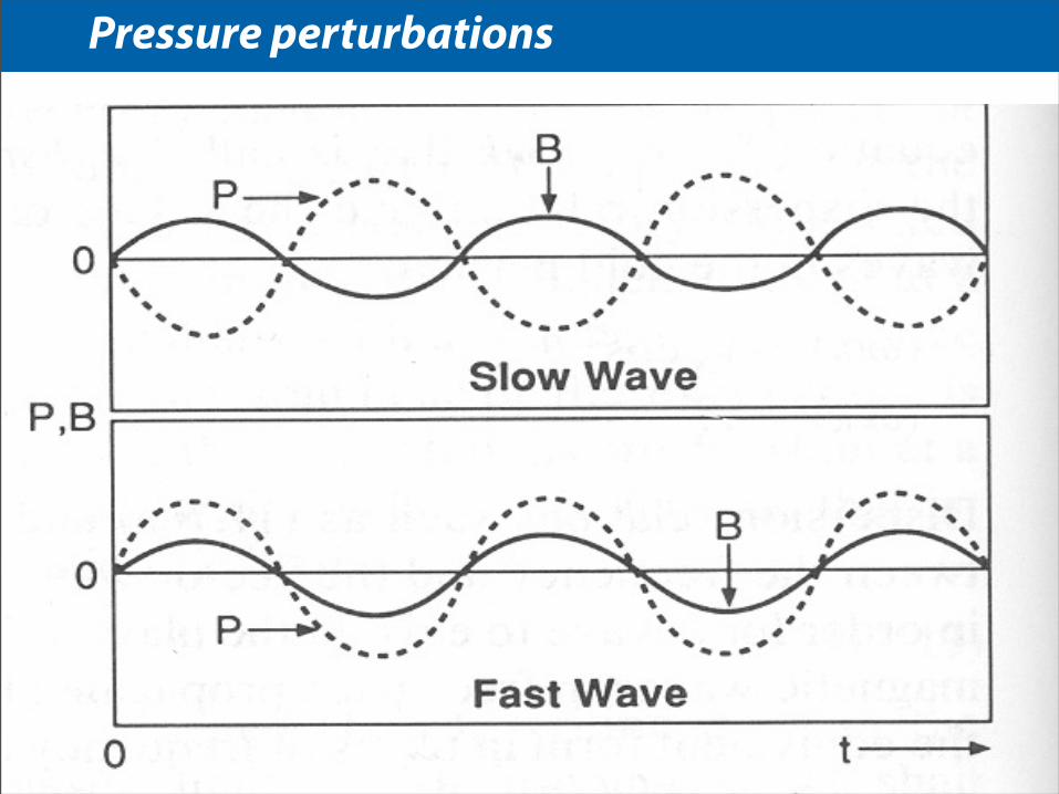
Pressure perturbations

Phase speeds:

: Group speeds

Phase and group speeds

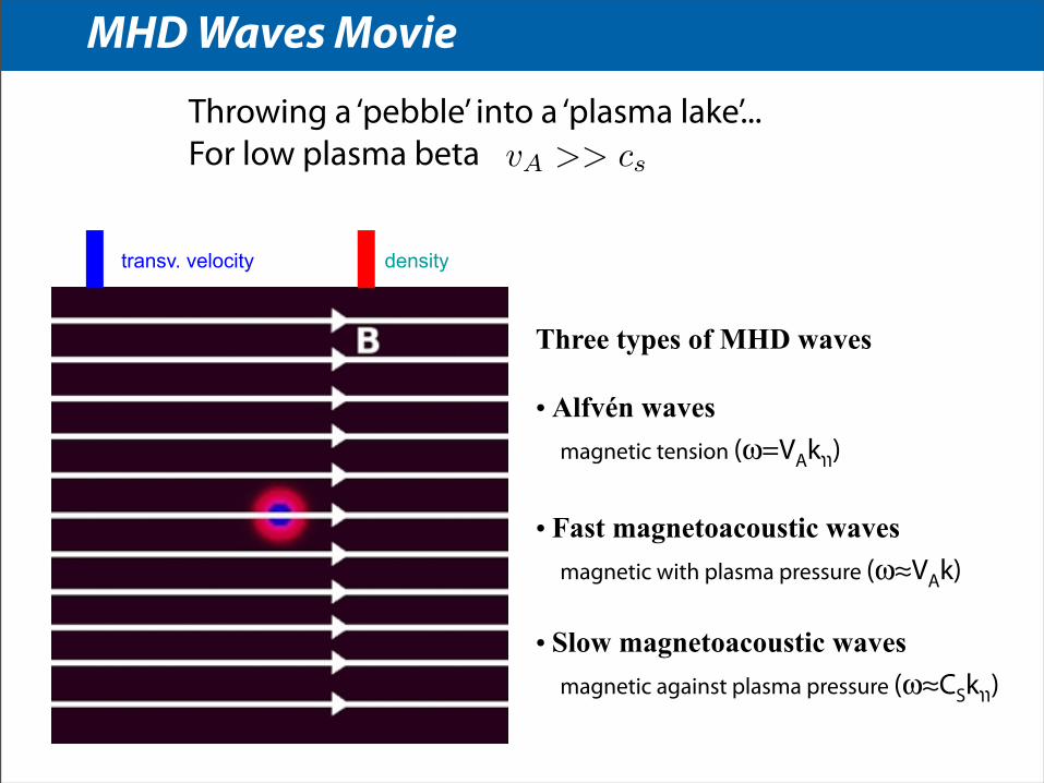
Throwing a ‘pebble’ into a ‘plasma lake’...For low plasma beta

Three types of MHD waves

• Alfvén waves magnetic tension (ω=VAkװ)

• Fast magnetoacoustic waves magnetic with plasma pressure (ω≈VAk)

• Slow magnetoacoustic waves magnetic against plasma pressure (ω≈CSkװ)

transv. velocity density

MHD Waves Movie

vA >> cs

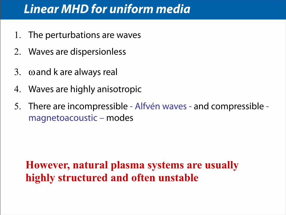
1. The perturbations are waves

2. Waves are dispersionless

3. ω and k are always real

4. Waves are highly anisotropic

5. There are incompressible - Alfvén waves - and compressible - magnetoacoustic – modes

However, natural plasma systems are usually highly structured and often unstable

Linear MHD for uniform media

Non-ideal terms in MHD

Ideal MHD is a set of conservation laws

Non-ideal terms are dissipative and entropy producing

• Resistivity• Viscosity• Radiation transport• Thermal conduction

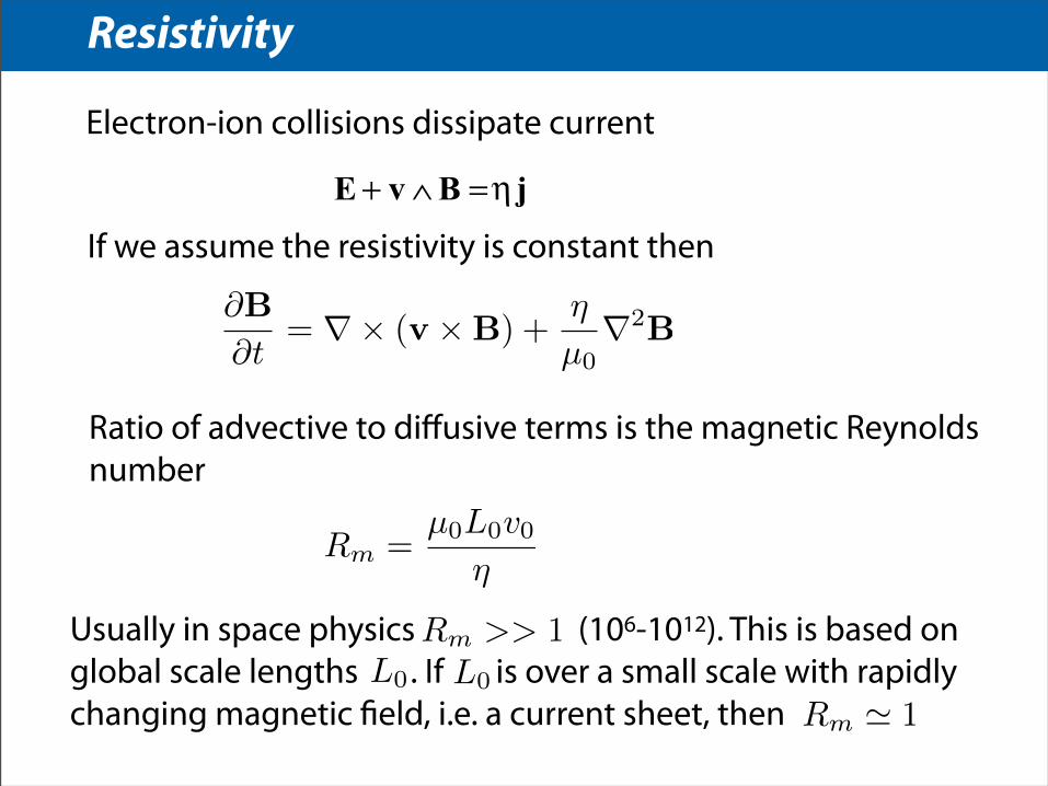
Resistivity

Electron-ion collisions dissipate current

@B

@t= r⇥ (v ⇥B) +

⌘

µ0r2B

If we assume the resistivity is constant then

Ratio of advective to diffusive terms is the magnetic Reynolds number

Rm =µ0L0v0

⌘

Usually in space physics (106-1012). This is based on global scale lengths . If is over a small scale with rapidly changing magnetic field, i.e. a current sheet, then

Rm >> 1

Rm ' 1L0 L0

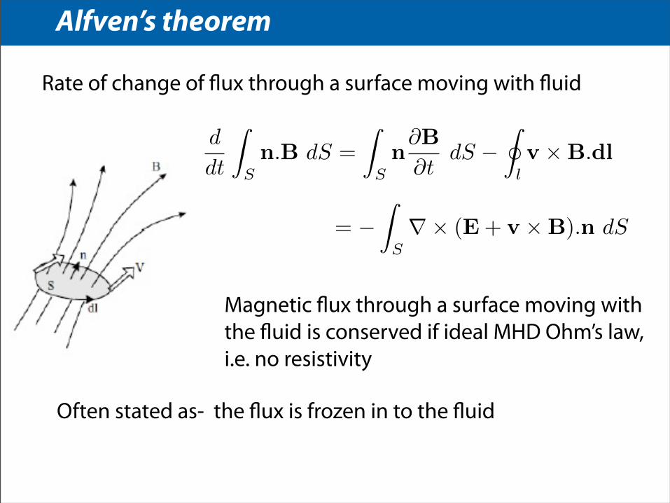
Alfven’s theorem

d

dt

Z

Sn.B dS =

Z

Sn@B

@tdS �

I

lv ⇥B.dl

= �Z

Sr⇥ (E+ v ⇥B).n dS

Rate of change of flux through a surface moving with fluid

Magnetic flux through a surface moving with the fluid is conserved if ideal MHD Ohm’s law, i.e. no resistivity

Often stated as- the flux is frozen in to the fluid

Line Conservation

x(X, t)

x(X+ �X, t)

�X

Consider two points which move with the fluid

�x

�xi =@xi

@Xj�Xj

x(X+ �X, 0)

x(X, 0) = X

=@ui

@xk

@xk

@xj�Xj

= (�x.r)u

D

Dt�x =

@ui

@Xj�Xj

Line Conservation -2

D

Dt�x = (�x.r)u

Equation for evolution of the vector between two points moving with the fluid is

D

Dt

✓B

⇢

◆=

B

⇢.rv

Also for ideal MHD

Hence if we choose to be along the magnetic field at t = 0 then it will remain aligned with the magnetic field.

Two points moving with the fluid which are initially on the same field-line remain on the same field line in ideal MHD

Reconnection not possible in ideal MHD

�x

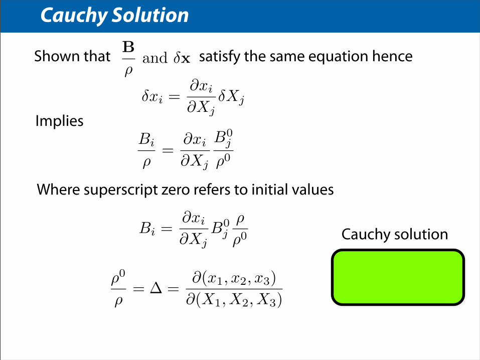
Cauchy Solution

Shown that satisfy the same equation hence B

⇢and �x

�xi =@xi

@Xj�Xj

ImpliesBi

⇢

=@xi

@Xj

B

0j

⇢

0

Where superscript zero refers to initial values

Bi =@xi

@XjB

0j⇢

⇢

0

⇢

0

⇢

= � =@(x1, x2, x3)

@(X1, X2, X3)

Bi =@xi

@Xj

B

0j

�

Cauchy solution

MHD based on Cauchy

Bi =@xi

@Xj

B

0j

�

⇢

0

⇢

= � =@(x1, x2, x3)

@(X1, X2, X3)

P = const ⇢

�

Dv

Dt= �1

⇢r.P +

1

µ0⇢(r⇥B)⇥B

Only need to know position of fluid elements and initial conditions for full MHD solution

dx

dt= v

Resistivity

Coriolis Gravity“Other”

Thermal

Conduction

Radiation Ohmic heating

“Other”

Non-ideal MHD

Sets of ideal MHD equations can be written as

All equations sets of this types share the same properties

• they express conservation laws

• can be decomposed into waves

• non-linear solutions can form shocks

• satisfy L1 contraction, TVD constraints

MHD Characteristics

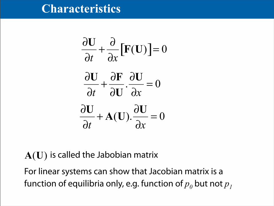
Characteristics

is called the Jabobian matrix

For linear systems can show that Jacobian matrix is a function of equilibria only, e.g. function of p0 but not p1

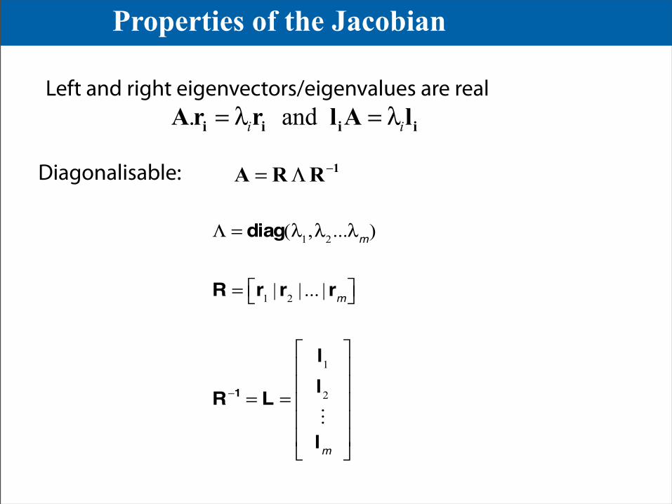
Properties of the Jacobian

Left and right eigenvectors/eigenvalues are real

Diagonalisable:

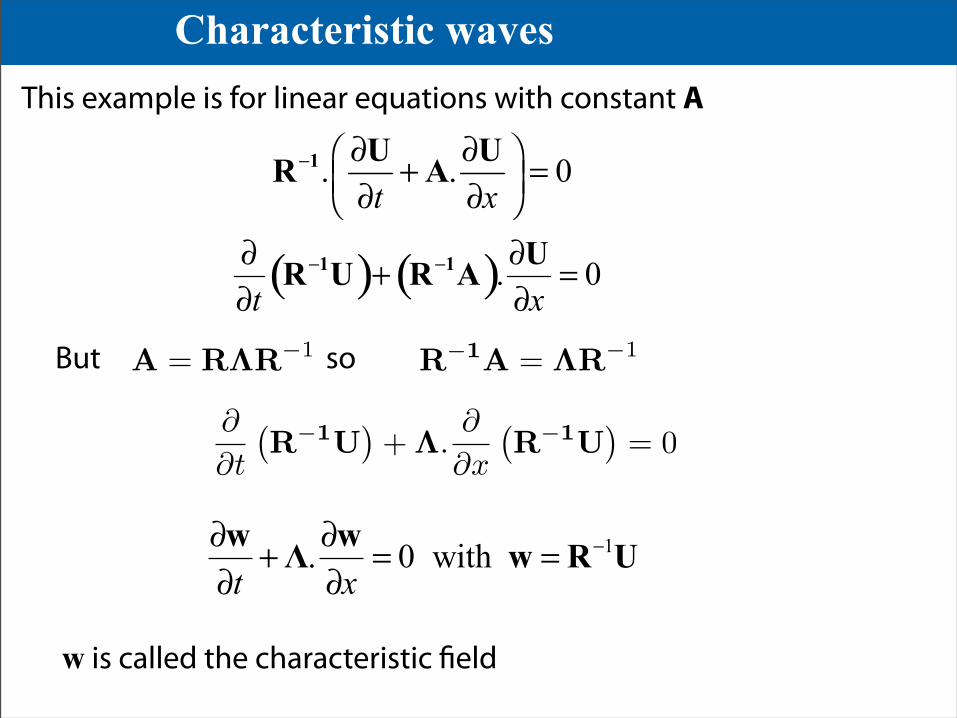
Characteristic waves

But

w is called the characteristic field

A = R⇤R�1 so R�1A = ⇤R�1

@

@t

�R�1U

�+⇤.

@

@x

�R�1U

�= 0

1. 0 with t x

−∂ ∂+ = =∂ ∂w wΛ w R U

This example is for linear equations with constant A

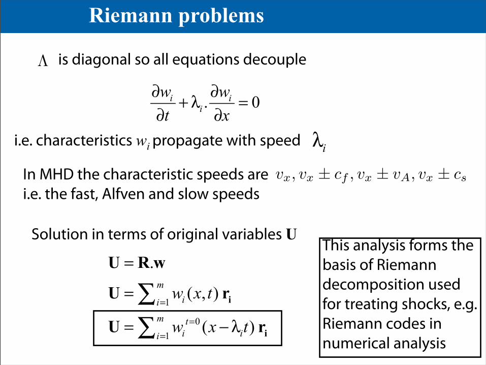
is diagonal so all equations decouple

i.e. characteristics wi propagate with speed

Solution in terms of original variables UThis analysis forms the basis of Riemann decomposition used for treating shocks, e.g. Riemann codes in numerical analysis

⇤

Riemann problems

In MHD the characteristic speeds are i.e. the fast, Alfven and slow speeds

vx

, vx

± cf

, vx

± vA

, vx

± cs

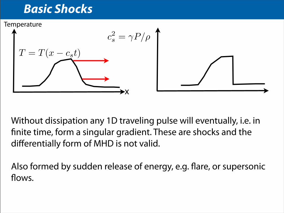
Basic ShocksTemperature

x

c2s = �P/⇢

T = T (x� cst)

Without dissipation any 1D traveling pulse will eventually, i.e. in finite time, form a singular gradient. These are shocks and the differentially form of MHD is not valid.

Also formed by sudden release of energy, e.g. flare, or supersonic flows.

Rankine-Hugoniot relations

U

xS(t)xrxl

UL

UR

Integrate equations from xl to xr across moving discontinuity S(t)

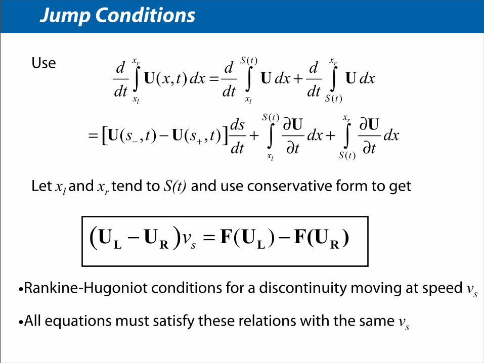
Use

Let xl and xr tend to S(t) and use conservative form to get

•Rankine-Hugoniot conditions for a discontinuity moving at speed vs

•All equations must satisfy these relations with the same vs

Jump Conditions

The End