UNIVERSITY OF TORONTO

Faculty of Arts and Science

JUNE EXAMINATIONS 2008

STA 302 H1F / STA 1001 H1F Duration - 3 hours

Aids Allowed: Calculator LAST NAME: FIRST NAME: STUDENT NUMBER: Enrolled in (Circle one): STA302 STA1001 There are 16 pages including this page. The last page is a table of formulae that may be useful. For all questions you can assume that the results on the formula page are known. Tables of the t and F distributions are attached. Total marks: 90 PLEASE CHECK AND MAKE SURE THAT THERE ARE NO MISSING PAGES IN THIS BOOKLET.

1) We want to fit the normal error regression model Y 0 1i X i iβ β ε= + +

i

with five observations with X = 1, 2, 3, 4, and 5. We know that ε ’s are independent and normally distributed with mean 0 and standard deviation σ = 2. a) [3] Calculate 1 1 1( 1 1P b b )β− ≤ ≤ + where is the least square estimator of 1b 1β .

Sol 2(XX iS X= −∑ )X =4+1+0+1+4 = 10 and Var∑

and

so ~ N(1b 1β , ) ( when sigma is known). Or use. Calculate these 2 20.1 2 0.4× =0.1 σ× =using the formulas for var and cov for b0 and b1 . This part only need the formula for var(b1) but the full xpx inv matrix is useful to answer part b.

2

1 2

4( ) 0.4( ) 10i

bX Xσ

= = =−

1 1 1 11 1 1

1 1( 1 1) ( ) ( 1.58 1.58)0.630.4 0.4 0.4

b bP b b P Pβ ββ − −−− ≤ ≤ + = ≤ ≤ = − ≤ ≤

= = 1- 0.0570534 *2 = 0.8858932 ( 1.58 1.58)P Z− ≤ ≤

1

b) [5] Calculate where 1( 1 1)P e− ≤ ≤ 1 1

ˆe Y Y= − is the residual for the first observation (i.e. at X =1). Sol

-1 1.1 -0.3( )

-0.3 0.1 ′ =

X X

1 1ˆe Y Y= − 1 ~ N( 0, (1 2

11)h σ− ) = N( 0 , 0.4 *4 = 1.6) and so where is the first 11h

diagonal element of the hat matrix. -1

0.6 0.4 0.2 0.0 -0.20.4 0.3 0.2 0.1 0.0

( ) 0.2 0.2 0.2 0.2 0.20.0 0.1 0.2 0.3 0.4

-0.2 0.0 0.2 0.4 0.6

′ ′ =

X XX X where

1 11 21 31 41 5

=X

.

2

Note: You only need to calculate the first diagonal element of H. I got the full H because I just used my computer to get it.

11 1( 1 1) ( ) ( 0.79 0.79)

1.6 1.6P e P Z P Z−− ≤ ≤ = ≤ ≤ = − ≤ ≤

= 1 - 2*0.214764 = 0.570472 2) Consider the linear regression model in matrix form that we discussed in class:

where X is an matrix with the first column containing all 1’s and has rank p (and so (X exists), and is a vector of uncorrelated errors with covariance matrix

= +Y Xβ ε

2

n p×1′ -X) ε

σ I . Let ˆ X=Y b where 1( )−′ ′b X X X= Y

H

is the vector of least squares regression estimates. You may any result we proved in class (other than of course the result the question wants you to prove). a) [2] Show that where 2ˆ( )Cov σ=Y -1( )′ ′H = X X X X b) [5] Let . Show that 0( )ijh=H 1iih≤ ≤ for i n1, ,= … . Sol To prove , note that Var1iih ≤ 2( ) (1 ) 0 1i ii iie h hσ= − ≥ ⇒ ≤

To prove , consider 0iih ≥ i i H′= aα where a_i is an nx1 vector with all components 0 except the ith element which is 1. 0i i′ ≥α α (this is the sum of squares of elements of α ) i

and α α i i′ iih= 3) Systolic blood pressure readings of individuals are thought to be related to weight and age. The following SAS outputs were obtained from a regression analysis of systolic blood pressure on weight (in pounds). The REG Procedure Model: MODEL1 Dependent Variable: Systolic

3

Analysis of Variance Sum of Mean Source DF Squares Square F Value Pr > F Model 1 162.75422 162.75422 8.11 0.0147 Error 12 240.74578 20.06215 Corrected Total 13 403.50000 Parameter Estimates Parameter Standard Variable DF Estimate Error t Value Pr > |t| Intercept 1 128.93469 omitted omitted omitted Weight 1 0.13173 omitted omitted omitted (a) State whether the following statements are true or false. Circle your answer. [1 point for each part] i) More than 60% of the variation in systolic blood pressure has been accounted for by the linear relationship with weight. (True / False) Ans F. R-sq = 162.75422/403.50000 =

0.4033561834, 40.3% ii) The margin of error of the 90% confidence interval for 1β (the population regression coefficient of weight) is greater than 0.15. (True / False) Ans F. 90 % CI does not include 0 (because the p-value for testing beta1 = 0 is 0.0147 (from the ANOVA table) < 0.10 (the alpha for 90%confidence). The centre of the CI is the estimated beta1 = 0.132 and so the distance between the centre and the lower end point of the interval (I’e’ the margin of error) is, less than 0.132 –0 =0.132. You can also calculate it using t = sqrt(8.11) = 2.847806173 and so SE = 0.132/2.847806173 = 0.04635146916 and ME = = 1.782*0.04635146916 =0.08259831804 *t SE (b) [3] The least squares regression equation of systolic blood pressure on weight and age calculated from the same group of individuals was: Systolic = 125 + 0.119 Weight + 0.104 Age with R-Sq = 40.9%. Test the null hypothesis 0 : ageH 0β = against the alternative : 0a ageH β ≠ , where ageβ is the population regression coefficient of Age. Use α = 0.05. Show your workings clearly. F table p 667 Sol use R-sq to calculate ssR(x1 x2)=R-sq*SST. SSR (x1) is given and use F(drop) (partial F test) SSE (F) can also be found from R-sq= 1 –SSE/SST since SST is given F = 2.19/21.69 = 0.1009681881 T = 0.3177549183 Here is the minitab output for info (for comparing the above answer):

4

Regression Analysis: Systolic versus Weight, Age The regression equation is Systolic = 125 + 0.119 Weight + 0.104 Age Predictor Coef SE Coef T P Constant 125.08 15.35 8.15 0.000 Weight 0.11907 0.06243 1.91 0.083 Age 0.1037 0.3261 0.32 0.756 S = 4.65688 R-Sq = 40.9% R-Sq(adj) = 30.1% Analysis of Variance Source DF SS MS F P Regression 2 164.95 82.47 3.80 0.056 Residual Error 11 238.55 21.69 Total 13 403.50 Source DF Seq SS Weight 1 162.75 Age 1 2.19

4) [8] In a simple linear regression analysis of the relationship between fuel efficiency (Y, in gallons per 100 miles) and the weight (X, in 1000s of pounds) of cars , the researchers collected data on n = 38 cars. Some summary statistics of the data and the scatterplot of Y versus X are given below:

2.863X = , 0.707XS =

4.331Y = , 1.156YS =The MSE for the simple linear regression of Y on X is 0.195.

X

Y

4.54.03.53.02.52.0

7

6

5

4

3

Scatterplot of Y vs X

Calculate the least square estimates of 0β and 1β , and their standard errors (i.e. and

) for the simple linear regression model 0bs

1bs 0 1iY Xi iβ β ε= + + , satisfying the usual assumptions. Show your workings clearly.

5

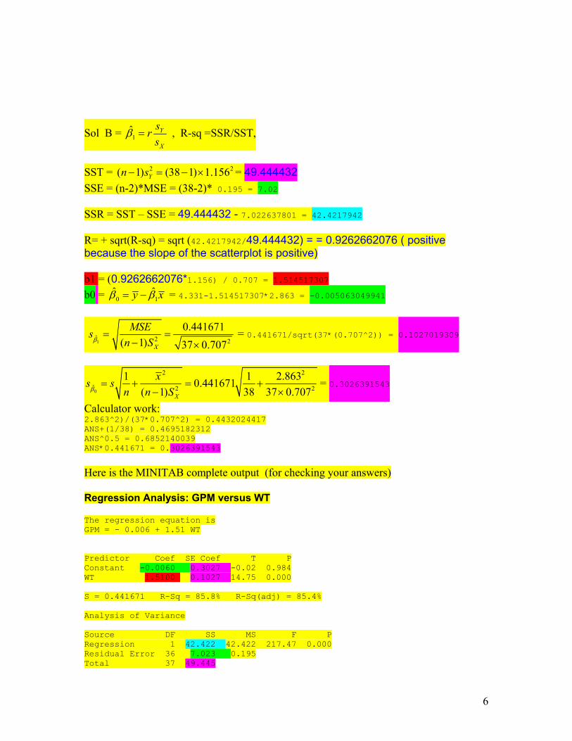
Sol B = 1̂Y

X

srs

β = , R-sq =SSR/SST,

SST = = 49.444432 2 2( 1) (38 1) 1.156Yn s− = − ×SSE = (n-2)*MSE = (38-2)* 0.195 = 7.02 SSR = SST – SSE = 49.444432 - 7.022637801 = 42.4217942 R= + sqrt(R-sq) = sqrt (42.4217942/49.444432) = = 0.9262662076 ( positive because the slope of the scatterplot is positive) b1 = (0.9262662076*1.156) / 0.707 = 1.514517307 b0 = 0

ˆ y 1̂xβ β= − = 4.331-1.514517307*2.863 = -0.005063049941

1̂ 2 2

0.441671( 1) 37 0.707X

MSEn Sβ

= =− ×

s = 0.441671/sqrt(37*(0.707^2)) = 0.1027019309

0

2 2

ˆ 2 2

1 1 2.8630.441671( 1) 38 37 0.707X

xs sn n Sβ

= + = +− ×

= 0.3026391543

Calculator work: 2.863^2)/(37*0.707^2) = 0.4432024417 ANS+(1/38) = 0.4695182312 ANS^0.5 = 0.6852140039 ANS*0.441671 = 0.3026391543 Here is the MINITAB complete output (for checking your answers) Regression Analysis: GPM versus WT The regression equation is GPM = - 0.006 + 1.51 WT Predictor Coef SE Coef T P Constant -0.0060 0.3027 -0.02 0.984 WT 1.5100 0.1027 14.75 0.000 S = 0.441671 R-Sq = 85.8% R-Sq(adj) = 85.4% Analysis of Variance Source DF SS MS F P Regression 1 42.422 42.422 217.47 0.000 Residual Error 36 7.023 0.195 Total 37 49.445

6

5)[5] After fitting the normal error regression model Y 0 1i X i iβ β ε= + + satisfying usual assumptions t on n = 6 observations, the fitted values were calculated (i.e. ’s) and are given with the data on X and Y in the following table:

ˆiy

x y ˆiy 1 1 0.85714 2 2 1.71429 3 2 2.57143 4 3 3.42857 5 5 4.28571 6 5 5.14286

You may also use these summary statistics if you need 3.5X = , , 1.871XS = 3Y = ,

. 1.673YS = Test the null hypothesis 0 1:H 0β = against the alternative 1 1:H 0β ≠ . Use a t-test with α = 0.05. Show your workings clearly. Sol x y FITS1 y-y^hat (y-y^hat)^2 1 1 0.85714 0.142857 0.020408 2 2 1.71429 0.285714 0.081633 3 2 2.57143 -0.571429 0.326531 4 3 3.42857 -0.428571 0.183673 5 5 4.28571 0.714286 0.510204 6 5 5.14286 -0.142857 0.020408 SSE = total of the (y-y^hat)^2 column = 1.1429 Descriptive Statistics: (y-y^hat)^2 Variable Sum (y-y^hat)^2 1.1429

SST = (n – 1)*var(y) = (6-1)* 1.673^2 = 13.994645 SSR = SST –SSE = 13.994645 - 1.1429= 12.851745 = SSR as well F = MSR/MSE = 12.851745/(1.1429/(6-2)) = 44.97942077 T = sqrt(44.98) = 6.706713055

7

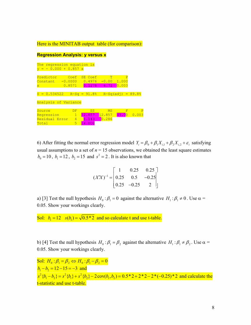
Here is the MINITAB output table (for comparison): Regression Analysis: y versus x The regression equation is y = - 0.000 + 0.857 x Predictor Coef SE Coef T P Constant -0.0000 0.4976 -0.00 1.000 x 0.8571 0.1278 6.71 0.003 S = 0.534522 R-Sq = 91.8% R-Sq(adj) = 89.8% Analysis of Variance Source DF SS MS F P Regression 1 12.857 12.857 45.00 0.003 Residual Error 4 1.143 0.286 Total 5 14.000

i6) After fitting the normal error regression model Y X0 1 ,1 2 ,2i i iXβ β β ε= + + + satisfying

usual assumptions to a set of n = 15 observations, we obtained the least square estimates , b , and 0 10b = 1 12= 2 15b = 2 2s = . It is also known that

1

1 0.25 0.25( ) 0.25 0.5 0.25

0.25 0.25 2X X −

′ = − −

a) [3] Test the null hypothesis 0 1:H 0β = against the alternative 1 1:H 0β ≠ . Use α = 0.05. Show your workings clearly. Sol: b 1 12= 1( ) 0.5*2s b = and so calculate t and use t-table. b) [4] Test the null hypothesis 0 1:H 2β β= against the alternative 1 1:H 2β β≠ . Use α = 0.05. Show your workings clearly. Sol: 0 1 2 0 1 2: :H H 0β β β β= ⇔ − =

1 2 12 15 3b b− = − = − and 2 2 2

1 2 1 2 1 2{ } { } { } 2cov( , ) 0.5*2 2*2 2*( 0.25)*2s b b s b s b b b− = + − = + − − and calculate the t-statistic and use t-table.

8

c)[3] Calculate a 95% confidence interval for 0 12 1β β− + . 7) The SAS output below was obtained from a study of the relationship between the height (feet) and the diameter (inches) of sugar maple trees (Johnson, R. A. and Bhattacharyya, G. K, 2006). In the output below, y = height in feet, x = diameter in inches of the sugar maple trees and _x sq x x= × . The SAS System The REG Procedure Model: MODEL1 Dependent Variable: y Analysis of Variance Sum of Mean Source DF Squares Square F Value Pr > F Model 2 5214.01734 2607.00867 33.78 <.0001 Error 9 694.49183 77.16576 Corrected Total 11 5908.50917 Parameter Estimates Parameter Standard Variable DF Estimate Error t Value Pr > |t| Intercept 1 17.56905 5.38148 3.26 0.0098 x 1 6.65128 1.26819 5.24 0.0005 x_sq 1 -0.15846 0.04874 -3.25 0.0100

We convert the units of diameter (x) from inches to cm (assume that 1 inch = 2.54 cm) and the units of height (y) from feet to meters (assume that 1 foot = 0.3 m). Let denote the height in meters and

y′x′y′

denote the diameter in cm. Most of the useful information for the regression model of on x′ and _x sq′ , where _x sq x x′ ′ ′= × , can be calculated from the information on the SAS output given above (for the regression of y on x, and x_sq) i) [3] Give the estimated least square regression equation for y′on x′ and _x sq′ .

= (6.65/2.54)*0.3 = 0.7854330709

Ans: where 0 1 2ˆ ˆ ˆ _y x xβ β β′ ′ ′= + + sq 0β̂ = 17.6*0.3 = 5.28

1̂β

2β̂ =( - 0.158/(2.54^2))*3 = 0.007347014694

9

ii) [2] Calculate the SSE for the transformed model. (i.e. the model for on y′ x′ and _x sq′ .)

Ans 694.5 *(0.3^2) = 62.505 Here is the MINITAB output for the transformed data (for comparing your answers) : Regression Analysis: y versus x, x_sq The regression equation is y = 17.6 + 6.65 x - 0.158 x_sq Predictor Coef SE Coef T P Constant 17.569 5.381 3.26 0.010 x 6.651 1.268 5.24 0.001 x_sq -0.15846 0.04874 -3.25 0.010 S = 8.78440 R-Sq = 88.2% R-Sq(adj) = 85.6% Analysis of Variance Source DF SS MS F P Regression 2 5214.0 2607.0 33.78 0.000 Residual Error 9 694.5 77.2 Total 11 5908.5 Regression Analysis: ty versus tx, tx_sq The regression equation is ty = 5.27 + 0.786 tx - 0.00737 tx_sq Predictor Coef SE Coef T P Constant 5.271 1.614 3.26 0.010 tx 0.7856 0.1498 5.24 0.001 tx_sq -0.007368 0.002266 -3.25 0.010 S = 2.63532 R-Sq = 88.2% R-Sq(adj) = 85.6% Analysis of Variance Source DF SS MS F P Regression 2 469.26 234.63 33.78 0.000 Residual Error 9 62.50 6.94 Total 11 531.77

8) A commercial real estate company evaluates vacancy rates, square footage, rental rates and operating expenses for commercial properties in a large metropolitan area. The SAS output below was obtained from a regression analysis of the rental rates (Y) on four explanatory variables X1 = age, X2 = operating expenses and taxes, X3 = vacancy rates and X4 = total square footage.

10

The SAS System The REG Procedure Model: MODEL1 Model Crossproducts X'X X'Y Y'Y Variable Intercept x1 x2 Intercept 81 637 784.74 x1 637 8529 6704.31 x2 784.74 6704.31 8136.4982 x3 6.56 33.55 52.9948 x4 13011295 119029605 135991170.57 y 1226.25 9415.1 12027.13425 Model Crossproducts X'X X'Y Y'Y Variable x3 x4 y Intercept 6.56 13011295 1226.25 x1 33.55 119029605 9415.1 x2 52.9948 135991170.57 12027.13425 x3 1.9796 1148419.57 100.5425 x4 1148419.57 3.0422535E12 205009973.13 y 100.5425 205009973.13 18800.62 The REG Procedure Model: MODEL1 Dependent Variable: y X'X Inverse, Parameter Estimates, and SSE Variable Intercept x1 x2 Intercept 0.2584381584 -0.000304811 -0.025105743 x1 -0.000304811 0.0003524211 -0.000209425 x2 -0.025105743 -0.000209425 0.0030875989 x3 -0.250832155 0.0031443364 0.0219107298 x4 1.2355527E-7 -4.310481E-9 -3.072159E-8 y 12.200585882 -0.142033644 0.28201653 X'X Inverse, Parameter Estimates, and SSE Variable x3 x4 y Intercept -0.250832155 1.2355527E-7 12.200585882 x1 0.0031443364 -4.310481E-9 -0.142033644 x2 0.0219107298 -3.072159E-8 0.28201653 x3 0.9138529849 -3.746468E-7 0.6193435035 x4 -3.746468E-7 1.48363E-12 7.9243019E-6 y 0.6193435035 7.9243019E-6 98.230593943

a) [3] Calculate a 95% confidence interval for 4β , the population regression coefficient of X4 in the regression model for Y with the three predictors X1, X2, X3 and X4. Sol

11

b4 is given in the X'X Inverse, Parameter Estimates, and SSE above. (also SSE and n , n in the X'X X'Y Y'Y matrix, the 1st matrix. S(b4) is the 4th diagonal element of the X'X X'Y Y'Y above.

b) [5] Test the null hypothesis 0 1 3 4: 0H β β β= = =

3 4 , is not equal to 0 against

1 1: at least one of , or H β β β . Use α = 0.05. Sol SSE(F) is given in the X'X Inverse, Parameter Estimates, and SSE matrix (the last diag element. 98.230593943.and so SSR (F) = SST –SSE. SST = Y’Y – nY_bar^2. The reduced model is the simple linear reg model with x2 only and SS= b1^2.ssx2x2 = ssx2y^2/ssx2x2 . ssx2y = sum of x2_i*y_i- n x_bar*-y_bar., ssxx = sum of x2_i*x2_i- n x2_bar^2, These SS’s are in the first matrix above. I.e Model Crossproducts X'X X'Y Y'Y

9) A company designing and marketing lighting fixtures needed to develop forecasts of sales (.SALES = total monthly sales in thousands of dollars). The company considered the following predictors: ADEX = adverting expense in thousands of dollars MTGRATE = mortgage rate for 30-year loans (%) HSSTARTS = housing starts in thousands of units The company collected data on these variables and the SAS outputs below were obtained from this study. The SAS System The CORR Procedure 4 Variables: SALES ADEX MTGRATE HSSTARTS Simple Statistics Variable N Mean Std Dev Sum SALES 46 1631 400.36378 75041 ADEX 46 154.97826 89.22369 7129 MTGRATE 46 8.48152 1.01403 390.15000 HSSTARTS 46 97.23696 20.97182 4473

12

Pearson Correlation Coefficients, N = 46 Prob > |r| under H0: Rho=0 SALES ADEX MTGRATE HSSTARTS SALES 1.00000 0.56098 -0.67732 0.82725 <.0001 <.0001 <.0001 ADEX 0.56098 1.00000 -0.80389 0.26731 <.0001 <.0001 0.0725 MTGRATE -0.67732 -0.80389 1.00000 -0.34973 <.0001 <.0001 0.0172 HSSTARTS 0.82725 0.26731 -0.34973 1.00000 <.0001 0.0725 0.0172 The SAS System The REG Procedure Model: MODEL1 Dependent Variable: SALES Parameter Estimates Parameter Standard Variable DF Estimate Error t Value Pr > |t| Type I SS Intercept 1 1612.46147 432.34267 3.73 0.0006 122416341 ADEX 1 0.32736 0.43919 0.75 0.4602 2269959 MTGRATE 1 -151.22802 39.74780 -3.80 0.0005 1044647 HSSTARTS 1 12.86316 1.18625 10.84 <.0001 2872464

a) [5] Test the null hypothesis 0 : 0ADEX HSSTARTSH β β= =

is not equal to 0HSSTARTS

against

1 : at least one of or ADEXH β β where ADEXβ and HSSTARTSβ are the population regression coefficients of ADEX and HSSTARTS respectively in the model 0[ ] ADEXE SALES MTGRATEADEX HSSE TARTSMTGRAT HSSTARTSβ β β× + × β ×= + + . Use α = 0.05. Sol SSR (F) = sum f the type 1 SS. The SLR model SALES on MGRATE is the reduced model and for that model R-sq = 0.67732^2 = 0.4587623824 and SSR = R-sq *SST. SST =variance (Y) * (n-1)

b) [4] Let us now consider the simple linear regression model 0 1[ ]E SALES MTGRATEβ β= + × for predicting SALES based on MTGRATE only.

Calculate a 95% confidence interval for 1β in this model. Sol b1= r (sales, mtgate)*(s_sales/s_mtgrate) S(b1) = sqrt(MSE (MTGRATE)/sxx) Sxx =(n-1) * var(MTGRATE)

13

MSE = SSE/(n-2). SSE =SST – SSR SSR = R-sq *SST. SST =variance (Y) * (n-1)

b1 and the s(1b) are in the minitab output for the solution for part (a) above. 10) An experiment was conducted to compare the amounts of tar (in milligrams) passing through three types of cigarette filters. Ten cigarettes were selected at random from each type and their tar contents were measured. The means and the standard deviations of the three samples are given below. Assume that there are no serous violations in the assumptions needed for the statistical methods involved. Variable Type N Mean StDev Tar 1 10 12.689 2.034 2 10 18.282 2.614 3 10 16.248 2.860

Consider the model 0 1 1 2Ey x x2β β β= + + where y is the tar content. The variables 1x and

2x are indicator (dummy) variables identifying the type of cigarette filters and are defined as follows:

1x = 1 if type 1 and 0 otherwise

2x = 1 if type 2 and 0 otherwise a) [2] Calculate the value of the least squares estimate of 1β ? Show your workings clearly. Sol b0 = ybar3= 16.25 Ybar1=b0+b1 and so b1 =12.698 - 16.248 = -3.55 Ybar3 =b0+b2 and so b2 = 18.282 -16.248 = 2.034 Here is the MINITAB output fro checking your answers Descriptive Statistics: Tar Variable Type N Mean StDev Tar 1 10 12.689 2.034 2 10 18.282 2.614 3 10 16.248 2.860 Regression Analysis: Tar versus x1, x2 The regression equation is Tar = 16.2 - 3.56 x1 + 2.03 x2

14

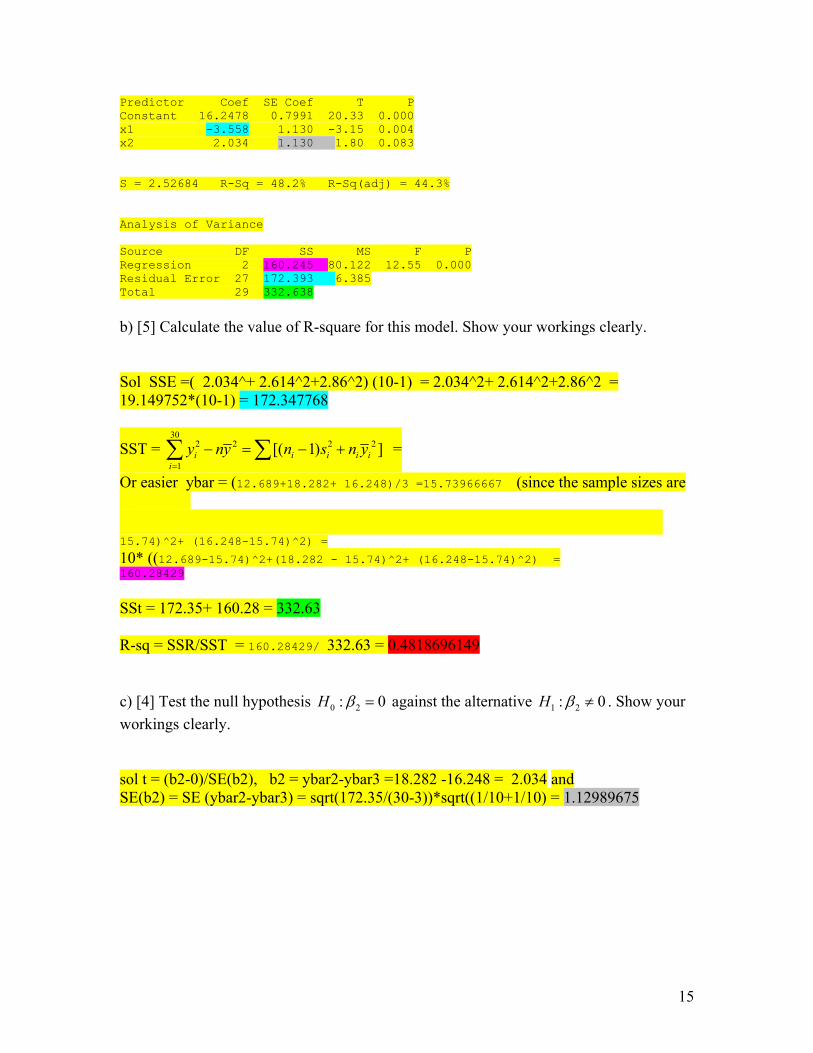
Predictor Coef SE Coef T P Constant 16.2478 0.7991 20.33 0.000 x1 -3.558 1.130 -3.15 0.004 x2 2.034 1.130 1.80 0.083 S = 2.52684 R-Sq = 48.2% R-Sq(adj) = 44.3% Analysis of Variance Source DF SS MS F P Regression 2 160.245 80.122 12.55 0.000 Residual Error 27 172.393 6.385 Total 29 332.638

b) [5] Calculate the value of R-square for this model. Show your workings clearly. Sol SSE =( 2.034^+ 2.614^2+2.86^2) (10-1) = 2.034^2+ 2.614^2+2.86^2 = 19.149752*(10-1) = 172.347768

SST = 30

2 2 2

1[( 1) ]i i i

iy ny n s n y

=

− = − +∑ ∑ 2i i =

Or easier ybar = (12.689+18.282+ 16.248)/3 =15.73966667 (since the sample sizes are equal) and SSR = 2 2

1 2 3) 10( ) 10( )y y y y y y− + − + − 2 =10( 10*( (12.689-15.74+18)^2+(18.282 – 15.74)^2+ (16.248-15.74)^2) = 10* ((12.689-15.74)^2+(18.282 - 15.74)^2+ (16.248-15.74)^2) = 160.28429 SSt = 172.35+ 160.28 = 332.63 R-sq = SSR/SST = 160.28429/ 332.63 = 0.4818696149 c) [4] Test the null hypothesis 0 2:H 0β = against the alternative 1 2:H 0β ≠ . Show your workings clearly. sol t = (b2-0)/SE(b2), b2 = ybar2-ybar3 =18.282 -16.248 = 2.034 and SE(b2) = SE (ybar2-ybar3) = sqrt(172.35/(30-3))*sqrt((1/10+1/10) = 1.12989675

15

11) The following SAS output was obtained from a study to identify the best set of predictors of sales for a company using data obtained from a random sample of n = 25 sales territories of the company. The variables in the SAS output below are defined as follows: SALES = sales (in units) for the territory TIME = length of time territory salesperson has been with the company POTENT = industry sales (in units) for the territory ADV = expenditures (in dollars) on advertising SHARE = weighted average of past market share for the last four years The REG Procedure Model: MODEL1 Dependent Variable: SALES R-Square Selection Method Number in Model R-Square Variables in Model 1 0.3880 TIME 1 0.3574 POTENT 1 0.3554 ADV 1 0.2338 SHARE ----------------------------------------------- 2 0.7461 POTENT SHARE 2 0.6071 POTENT ADV 2 0.5953 TIME ADV 2 0.5642 TIME SHARE 2 0.5130 TIME POTENT 2 0.4696 ADV SHARE ----------------------------------------------- 3 0.8490 POTENT ADV SHARE 3 0.8121 TIME POTENT SHARE 3 0.6991 TIME POTENT ADV 3 0.6959 TIME ADV SHARE ----------------------------------------------- 4 0.8960 TIME POTENT ADV SHARE Even though this output is from the R-square selection method, it has enough information that can be used in other selection methods. a) [3] What variable (if any) will be selected at the first step if we use the stepwise selection method? Use α = 0.10 to show whether the variable will enter the model or not. Show your working clearly. Sol: TIME because it has the highest Rsq among all the single variable models. Also for TIME F= R-sq/1/.[(1-R-sq)/(25 – 2) ]= 0.3880 /[(1-0.3880)/23] = 14.58 0.3880 /((1-0.3880)/23) = 14.58169935 t = sqrt(4.58) = 3.81 sig at alpha = 0.10

16

b) [5] What variable (if any) will be selected at the second step if we use the stepwise selection method? ? Use α = 0.10 to show whether the variable will enter the model or not. Show your working clearly. Sol Note alpha for leaving (or staying ) is not required as our questions are asking only the fisrt two variables entering the model. TIME ADV because this has the highest t-ratio (or F_drop) among the two variable models with TIME as one variable. Note F_drop = [SSR(TIME X_k)-SSR(TIME)]/MSE(TIME,x_k) = [Rsq(TIME X_k)-Rsq(TIME)]/[1-R-sq(TIME,x_k] /(n-3) = (0.5953 - 0.3880 )/ ((1-0.5953)/(25-3)) = 11.26908821 sqrt(11.26908821) = 3.356946263 (just divide the numerator and the denominator by SST to see this) Form this wee see that for all models containing TIME this only depends on Rsq(TIME, x_k) and this (ie. F_drop and so the t-value for x_k) increases as Rsq(TIME, x_k) increases. Rsq(TIME, x_k) is max when x_k = ADV. And so ADV has the highest t-ratio among the models containing TIME.

Multiple-choice questions. Circle the most appropriate answer from the list of answers labeled A), B), C), D), and. E) (2 points for each question below) 12) In the term test and assignment 1, we analyzed the regression model with no constant tern for the case with a single predictor. Let us now consider the model with two predictors Y X1 ,1 2 ,2 , 1, ,i i i iX i nβ β ε= + + = … (with no constant term, i.e. no 0β ) with non-random X variables and the random errors iε ’s satisfying the usual assumptions. We estimate 1β and 2β using the method of least squares and calculate least squares

residuals . Which of the following statements regarding residuals are necessary true.

ˆi i ie Y Y= −

I) ∑ (i.e. the weighted sum of residuals, weighted by the values of the variable 11

0n

i iie X

=

=

1X is equal to 0)

II) ∑ (i.e. the weighted sum of residuals, weighted by the values of the variable 21

0n

i iie X

=

=

2X is equal to 0)

17

III) ∑ (i.e. the sum residuals is equal to 0) 1

0n

iie

=

=

A) only III is true B) only I and II are true C) only I and III are true D) only II and III are true E) all the three statements I, II and III are true.

Ans B. III is not necessarily true for the no constant model. I and II are true because ′ =e X 0 Here is an example Regression Analysis: y versus x1, x2 The regression equation is y = 1.62 x1 + 4.75 x2 Predictor Coef SE Coef T P Noconstant x1 1.6217 0.1549 10.47 0.000 x2 4.7504 0.5832 8.14 0.000 S = 11.0986 Analysis of Variance Source DF SS MS F P Regression 2 718732 359366 2917.42 0.000 Residual Error 19 2340 123 Total 21 721072 Descriptive Statistics: RESI1 Variable N Sum RESI1 21 -2.32 Data Display Row y x1 x2 RESI1 1 174.4 68.5 16.7 -16.0218 2 164.4 45.2 16.8 11.2899 3 244.2 91.3 18.2 9.6767 4 154.6 47.8 16.3 -0.3514 5 181.6 46.9 17.3 23.3577 6 207.5 66.1 18.2 13.8448 7 152.8 49.5 15.9 -3.0082 8 163.2 52.0 17.2 -2.8381 9 145.4 48.9 16.6 -12.7605

18

10 137.2 38.4 16.0 -1.0819 11 241.9 87.9 18.3 12.4156 12 191.1 72.8 17.1 -8.1955 13 232.0 88.4 17.4 5.9801 14 145.3 42.9 15.8 0.6704 15 161.1 52.5 17.8 -8.5993 16 209.7 85.7 18.4 -16.6916 17 146.4 41.3 16.5 1.0399 18 144.0 51.7 16.3 -17.2762 19 232.6 89.6 18.1 1.3087 20 224.1 82.7 19.1 -0.7516 21 166.5 52.3 16.0 5.6758

i i

13) A simple linear regression model Y 0 1i Xβ β ε= + + was fitted to a data set with 25 observations and the residuals were calculated for all 25 observations. The sum of 20 of these values (i.e. 20 residuals) was –6.08. What will be the sum of the remaining 5 residuals? Choose the interval that contains the answer.

A) (-10, -5) B) (-5, 0) C) (0, 5) D) (5, 10) E) none of the above intervals contains this value

Ans D The sum of all residuals (i.e. all 25 residuals) is 0. Since 20 of them have a sum of –6.08, the sum of the remaining 5, should be +6.08. (to make the sum of all to 0) 14) In a simple linear regression analysis of a dependent variable Y on an independent variable X, in based on 18 observations, the 95% confidence interval for 1β (i.e. the slope) was (1.8, 2.2). What is the value of the t-test statistic for testing the null hypothesis

0 1:H 0β = against the alternative 1 1: 0H β ≠ ?

A) it will be less than 5.0 B) it will be greater than 5.0 but less than 18.0 C) it will be greater than 18.0 but less than 28.0 D) it will be greater than 28.0 but less than 35.0 E) it will be greater than 35.0

Ans C ME=(2.2-1.8)/2 = 0.2

19

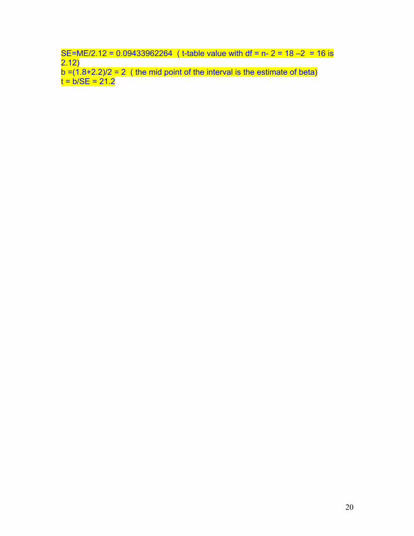
20

SE=ME/2.12 = 0.09433962264 ( t-table value with df = n- 2 = 18 –2 = 16 is 2.12) b =(1.8+2.2)/2 = 2 ( the mid point of the interval is the estimate of beta) t = b/SE = 21.2