UNIVERSITY OF MICHIGAN

DEPARTMENT OF ELECTRICAL ENGINEERING: SYSTEMS

PROJECT REPORT

FOR

EECS 555 DIGITAL COMMUNICATION THEORY

GUIDED BY

PROF. WAYNE STARK

ANALYSIS OF PHYSICAL LAYER PROPOSALS FOR IEEE P802.15a

BY

SHARMA SHRUTIVANADNA

SHEOREY SHRUTI

2

ACKNOWLEDGEMENT

It gives us immense pleasure to thank Professor W. Stark for his encouragement and dedication

to teaching us, which motivated us to work hard.

We are also obliged to be able to use the computer and internet facilities at the CAEN lab at

University of Michigan, which we used for running our simulations.

Last, but not least, we are thankful to our family and friends whose consistent support helped us

concentrate on our work.

3

INDEX

1. Abstract…………………………………………………………………………4

2. Introduction to Ultra Wide Band……………………………………………….4

3. Details of proposal for DS UWB physical layer……………………………….5

4. Details of proposal for MB-OFDM UWB physical layer……………………...8

5. Study of multipath channel models…………………………………………...11

6. Analysis of the proposal and Simulations…………………………………….15

7. Conclusion…………………………………………………………………….22

8. Bibliography…………………………………………………………………..+23

4

ABSTRACT

As the demand for in-home data communications rises, a need to find a means to send the information such that it can be recovered correctly becomes extremely demanding. UWB is an old technology considered for Personal Area Networks quite recently. In this project, two approaches to apply this technology are studied and analyzed.

1. Introduction to Ultra Wide Band Ultra Wide band signals are defined by FCC as the signals having bandwidth more than 25% of the center frequency or above 500 Hz. Particularly, they occupy bandwidth between 3.1 GHz to 10.6 GHz. Data rates vary from 28 to 1320Mbps. These low power and high bandwidth signals are particularly useful for transmitting signals over multipath channels. However, they are most efficient in a short range. As a result, they have enormous potential to be used in short range mobile applications or Personal Area Networks.

5

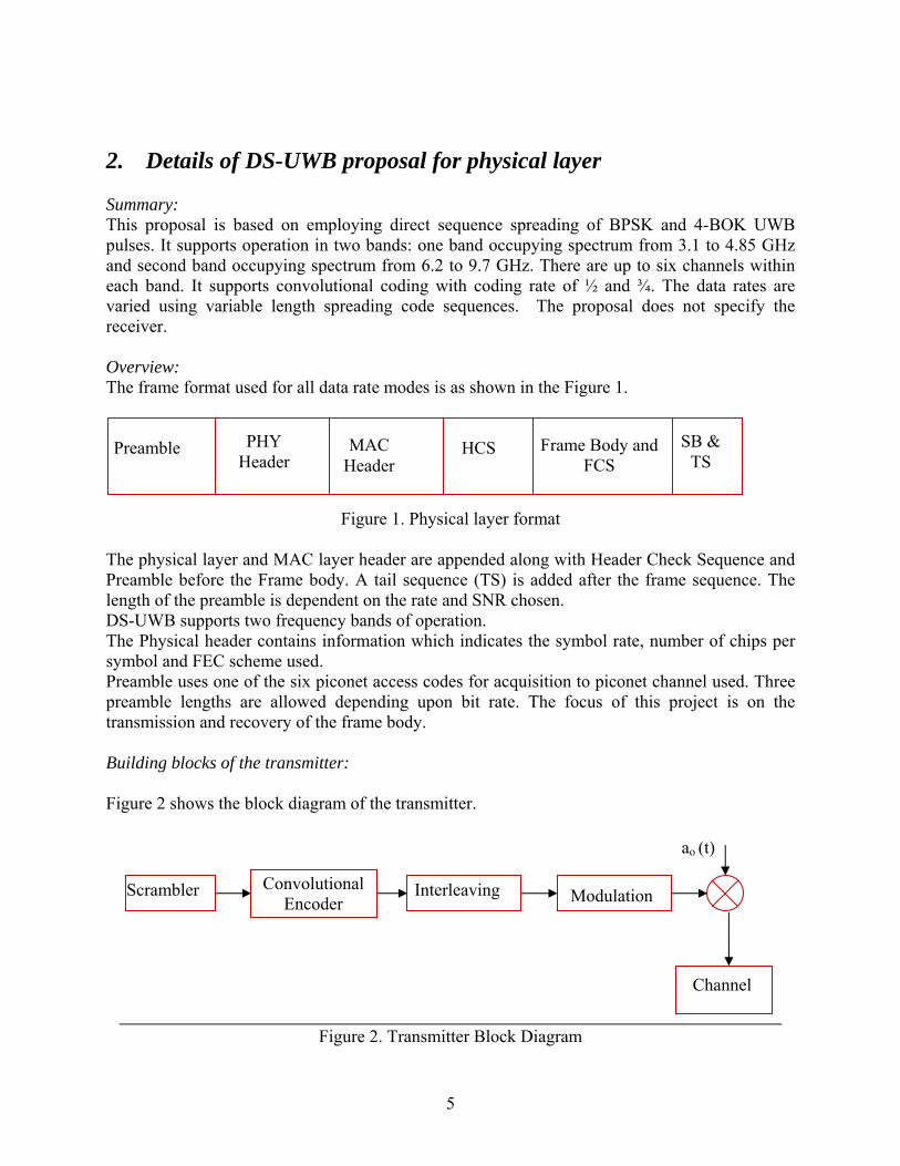
2. Details of DS-UWB proposal for physical layer Summary: This proposal is based on employing direct sequence spreading of BPSK and 4-BOK UWB pulses. It supports operation in two bands: one band occupying spectrum from 3.1 to 4.85 GHz and second band occupying spectrum from 6.2 to 9.7 GHz. There are up to six channels within each band. It supports convolutional coding with coding rate of ½ and ¾. The data rates are varied using variable length spreading code sequences. The proposal does not specify the receiver. Overview: The frame format used for all data rate modes is as shown in the Figure 1.

Figure 1. Physical layer format

The physical layer and MAC layer header are appended along with Header Check Sequence and Preamble before the Frame body. A tail sequence (TS) is added after the frame sequence. The length of the preamble is dependent on the rate and SNR chosen. DS-UWB supports two frequency bands of operation. The Physical header contains information which indicates the symbol rate, number of chips per symbol and FEC scheme used. Preamble uses one of the six piconet access codes for acquisition to piconet channel used. Three preamble lengths are allowed depending upon bit rate. The focus of this project is on the transmission and recovery of the frame body. Building blocks of the transmitter: Figure 2 shows the block diagram of the transmitter.

Figure 2. Transmitter Block Diagram

Preamble PHY Header

MAC Header

HCS Frame Body and FCS

SB & TS

Scrambler Convolutional Encoder

Interleaving Modulation

ao (t)

Channel

6

J

2J

(N-2)J

(N-1)J

Encoded bits

Interleaved bits

Scrambler

Figure 3 .Block diagram of the scrambler

Scrambler, as shown in Figure 3, is used to improve clock recovery at the receiver. If there are many zeros in the input to the receiver, it would not be able to locate the first bit. This could lead to synchronization problems. As a result, the transmitter uses scrambler to ‘scramble’ the data and produce uniform distribution of zeros in the output. The scrambler has a pseudo-random data generator having a generator polynomial and adds the data to the output of the generator. Generator polynomial used here is given by, g (D) =1 + D14 + D15 Convolutional encoder After the data is scrambled, it is passed through the encoder. Forward error correction would make the data robust against noise. It is followed by a puncturer. Puncturer is used to drop bits at regular duration and increase the rate of transmission. The parameters for the encoder are: Constraint length (K) = 4 Generator Polynomial (15, 17) Rate ½ or ¾ (punctured coding causes rate = ¾) Convolutional Interleaving Interleaving is employed to disperse the burst errors. It has lower latency and memory requirements than block interleaving. Figure 4 shows the working of the interleaver.

Figure 4. Convolutional Interleaver

……. D D D D bo

So

7

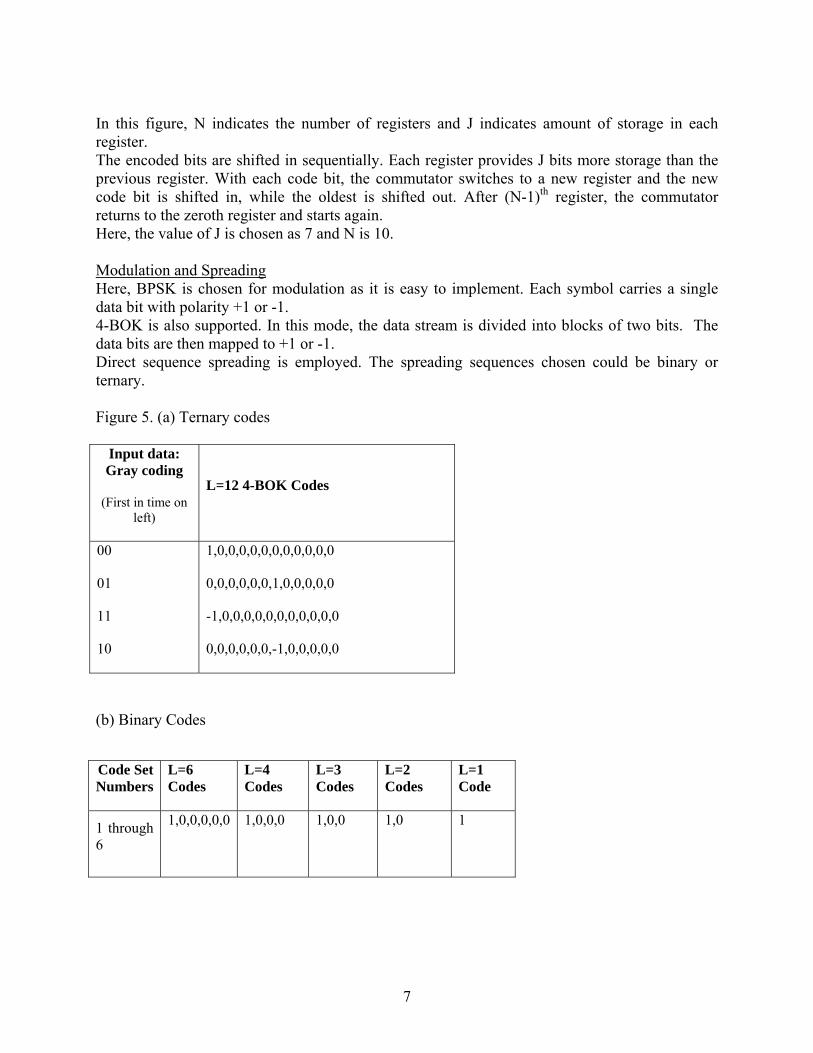
In this figure, N indicates the number of registers and J indicates amount of storage in each register. The encoded bits are shifted in sequentially. Each register provides J bits more storage than the previous register. With each code bit, the commutator switches to a new register and the new code bit is shifted in, while the oldest is shifted out. After (N-1)th register, the commutator returns to the zeroth register and starts again. Here, the value of J is chosen as 7 and N is 10. Modulation and Spreading Here, BPSK is chosen for modulation as it is easy to implement. Each symbol carries a single data bit with polarity +1 or -1. 4-BOK is also supported. In this mode, the data stream is divided into blocks of two bits. The data bits are then mapped to +1 or -1. Direct sequence spreading is employed. The spreading sequences chosen could be binary or ternary. Figure 5. (a) Ternary codes

Input data: Gray coding

(First in time on left)

L=12 4-BOK Codes

00

01

11

10

1,0,0,0,0,0,0,0,0,0,0,0

0,0,0,0,0,0,1,0,0,0,0,0

-1,0,0,0,0,0,0,0,0,0,0,0

0,0,0,0,0,0,-1,0,0,0,0,0

(b) Binary Codes

Code Set Numbers

L=6 Codes

L=4 Codes

L=3 Codes

L=2 Codes

L=1 Code

1 through 6

1,0,0,0,0,0

1,0,0,0

1,0,0

1,0

1

8

3. Details of MB-OFDM based UWB Physical Layer Summary This proposal is based on Orthogonal Frequency Division Multiplexing (OFDM). The system has 122 sub-carriers which are modulated using Quadrature Phase Shift Keying (QPSK). The data rates supported are 53.3,55, 80, 106.67, 110,160, 200, 320, 480 Mb/s. Convolutional Encoding is used with coding rates of 1/3, 11/32, 1/2, 5/8 and ¾. A time-frequency code is used to interleave coded data over three frequency bands. Overview The frame format used in this proposal is as shown in Figure 10.

Figure 10. Frame format for MB-OFDM based UWB.

The frame starts with a PLCP preamble. It is followed by a PLCP header which includes scrambler initializer, reserved bits, length and rate information. Then, tail bits, pad bits and MAC header are added followed by frame payload. FCS, tail bits and pad bits are appended to the frame payload. This project focuses on the frame payload transmission and reception. The data rates are varied using different FEC coding rates, conjugate symmetry of symbols and time domain spreading. Building blocks of MB-OFDM UWB based transmitter

Figure 11. Block diagram of MB-OFDM UWB based transmitter

Scrambler Convolutional Encoder

Block Interleaving

Modulation

Channel

Output

9

Figure 11 shows the block diagram of MB-OFDM UWB based transmitter. Scrambler Scrambler used is described in previous section. The generator polynomial used here is,

g (D) =1 + D14 + D15

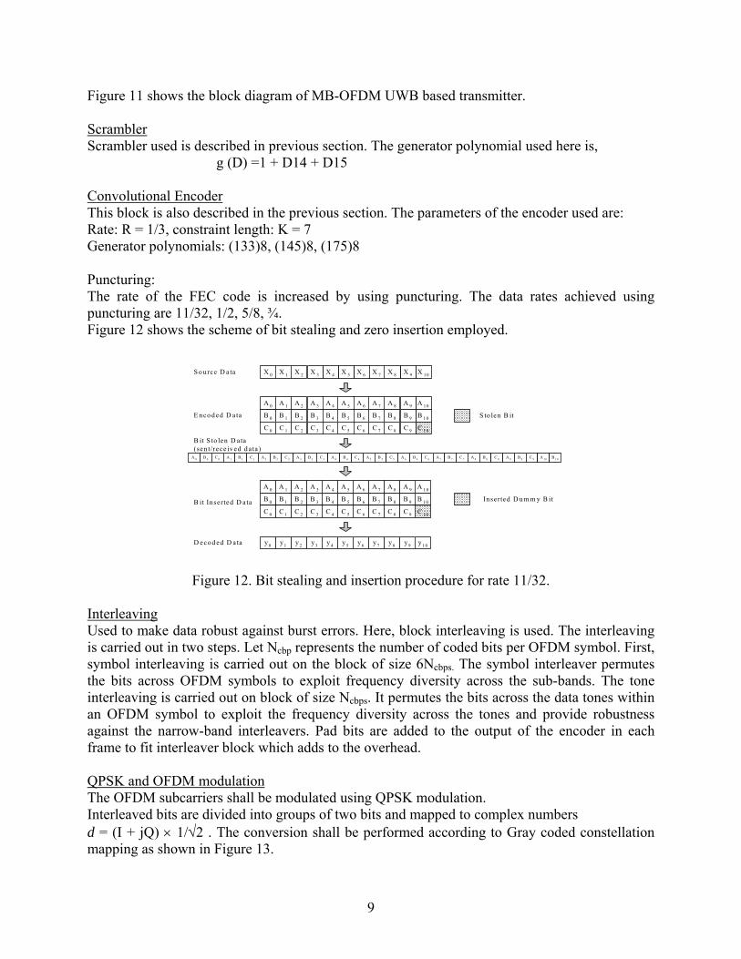
Convolutional Encoder This block is also described in the previous section. The parameters of the encoder used are: Rate: R = 1/3, constraint length: K = 7 Generator polynomials: (133)8, (145)8, (175)8 Puncturing: The rate of the FEC code is increased by using puncturing. The data rates achieved using puncturing are 11/32, 1/2, 5/8, ¾. Figure 12 shows the scheme of bit stealing and zero insertion employed.

Figure 12. Bit stealing and insertion procedure for rate 11/32.

Interleaving Used to make data robust against burst errors. Here, block interleaving is used. The interleaving is carried out in two steps. Let Ncbp represents the number of coded bits per OFDM symbol. First, symbol interleaving is carried out on the block of size 6Ncbps. The symbol interleaver permutes the bits across OFDM symbols to exploit frequency diversity across the sub-bands. The tone interleaving is carried out on block of size Ncbps. It permutes the bits across the data tones within an OFDM symbol to exploit the frequency diversity across the tones and provide robustness against the narrow-band interleavers. Pad bits are added to the output of the encoder in each frame to fit interleaver block which adds to the overhead. QPSK and OFDM modulation The OFDM subcarriers shall be modulated using QPSK modulation. Interleaved bits are divided into groups of two bits and mapped to complex numbers d = (I + jQ) × 1/√2 . The conversion shall be performed according to Gray coded constellation mapping as shown in Figure 13.

X 1 0X 9X 8X 7X 6X 5X 4X 3X 2X 1X 0

A 1 0A 9A 8A 7A 6A 5A 4A 3A 2A 1

B 1 0B 9B 8B 7B 6B 5B 4B 3B 2B 1B 0

C 1 0C 9C 8C 7C 6C 5C 4C 3C 2C 1C 0

A 1 0A 9A 8A 7A 6A 5A 4A 3A 2A 1A 0

B 10B 9B 8B 7B 6B 5B 4B 3B 2B 1B 0

C 10C 9C 8C 7C 6C 5C 4C 3C 2C 1C 0

y1 0y9y8y7y6y5y4y3y2y1y0

S to len B it

In se rted D um m y B it

A 0

A 0 B 0 C 0 A 1 B 1 C 1 A 2 B 2 C 2 A 3 B 3 C 3 A 4 B 4 C 4 A 5 B 5 C 5 A 6 B 6 C 6 A 7 B 7 C 7 A 8 B 8 C 8 A 9 B 9 C 9 A 1 0 B 1 0

S o urce D a ta

E nco d ed D ata

B it S to len D a ta(sen t/rece ived d ata )

B it Inserted D ata

D ecod ed D a ta

10

Figure 13. Constellation for QPSK modulation The complex numbers are divided into groups of 50 (conjugate symmetric) or 100. The orthogonal frequencies allocated are separated by ∆F = 528 MHz/ 128 = 4.125MHz. The allocation of sub-carrier frequency is as shown in figure 14.

Figure 14. Subcarrier frequency allocation Time domain spreading Time-domain spreading operation is performed with a spreading factor of 2 for data rates of 55, 80, 110, 160, 200 Mbps. The time-domain spreading operation consists of transmitting the same information over two OFDM symbols. These two OFDM symbols are transmitted over different sub-bands to obtain frequency diversity.

+ 1− 1

+ 1

− 1

Q

I

Q P S K

0 1 1 1

b 0 b 1

0 0 1 0

0 5 35

c4 9 c5 0 c5 3 P 5 c5 4 c8 0 P 3 5 c8 1D C

Subcarrier num bers

P -5 5c 0

-55 -45 -35

c 1 0 c1 8 P -3 5 c1 9 c2 7P -4 5c9c1

-25

P -2 5 c2 8

-15

P -1 5 c3 7c3 6

-5

P -5 c4 6c4 5

25

c 7 1 P 2 5 c7 2

15

c6 2 P 1 5 c6 3

45

c8 9 P 4 5 c 9 0

55

c9 8 P 5 5 c9 9

11

4. Study of Channel Models For usual narrow-band communications, it is possible to use Rayleigh as the fading model. However, in case of UWB systems, the paths separated by 133ps (which correspond to around 4cms) can be resolved by the receiver. As a result, the rays coming from the same object would also be resolved at the receiver. Moreover, since the bandwidth is large, there are very few multipaths which would overlap within each resolvable bin. Hence, we cannot apply the Central Limit Theorem and need to find some time-of-arrival statistics. The model proposed by IEEE 802.15 is based on S-V model. It defines clusters as the set of rays whose arrival is modeled as a Poisson process with rate Λ. Within each cluster, the arrival of rays is also modeled as a Poisson process with rate λ. The impulse response of the channel is given as,

where, {Tl

i} : delay of the lth cluster {τk, li} : delay of kth multipath component relative to lth cluster arrival time (Tli) {αk,li} : multipath gain coefficients {Xi} : lognormal shadowing, i : ith realization Tl = arrival time of the first path of lth cluster, Λ = cluster arrival rate τk,l = delay of kth path within lth cluster relative to Tl λ = ray arrival rate (within each cluster) The distribution of the cluster arrival time and ray arrival time is given by,

Channel co-efficients are given by,

The measurements were taken and it was found that the amplitude statistics matched with the lognormal distribution. Large-scale fading is also log-normally distributed.

where, μk,l is given by,

12

In above equations, ξl reflects the fading associated with the lth cluster, βk,l corresponds to fading associated with kth ray of the lth cluster. The shadowing term is given by,

The total multipath energy is contained in Xi. Assumptions made by the model: Ray and cluster arrival are independent of delay. Variance of log-normal fading is independent of delay. On the basis of this, the four channel measurement environments are given as, CM1 : LOS (less than 4 m). CM2 : NLOS (less than 4m) CM3 : NLOS (between 4-10m), CM4 : Strong delay dispersion, delay spread of 25ns. Figure: 15 CM1: Λ = 0.0233, λ = 2.5000, Γ = 7.1000, γ = 4.3000 σ1 = 3.3941, σ2 = 3.3941, σx = 3.0000, LOS

-2 0 2 4 6 8 10 12

x 10-8

0

0.1

0.2

0.3

0.4

0.5

0.6

0.7

0.8

time (seconds)

fain

g co

effic

ient

s

absolute value of Impluse response (CM1)

-2 0 2 4 6 8 10 12

x 10-8

-0.8

-0.6

-0.4

-0.2

0

0.2

0.4

0.6

time (seconds)

fain

g co

effic

ient

s

Impluse response (CM1)

13

Figure 16. CM2: Λ = 0.4000, λ = 0.5000, Γ = 5.5000, γ = 6.7000 σ1 = 3.3941, σ2 = 3.3941, σx = 3.0000,

Figure 17 CM3: Λ = 0.0667, λ = 2.1000, Γ = 14.0000, γ = 7.9000 σ1 = 3.3941, σ2 = 3.3941, σx = 3.0000, NLOS

-0.5 0 0.5 1 1.5 2 2.5

x 10-7

0

0.1

0.2

0.3

0.4

0.5

0.6

0.7

fain

g co

effic

ient

s

time (seconds)

absolute value of Impluse response (CM3)

-2 0 2 4 6 8 10 12 14

x 10-8

-0.2

-0.15

-0.1

-0.05

0

0.05

0.1

0.15

0.2

0.25

0.3Impluse response (CM2)

fain

g co

effic

ient

s

time (seconds)-2 0 2 4 6 8 10 12 14

x 10-8

0

0.05

0.1

0.15

0.2

0.25

0.3

0.35absolute value of Impluse response (CM2)

fain

g co

effic

ient

s

time (seconds)

-0.5 0 0.5 1 1.5 2 2.5

x 10-7

-0.3

-0.2

-0.1

0

0.1

0.2

0.3

0.4

0.5

0.6Impluse response (CM3)

fain

g co

effic

ient

s

time (seconds)

14

Figure 18 CM4: Λ = 0.0667, λ = 2.1000, Γ = 24.0000, γ = 12.0000 σ1 = 3.3941, σ2 = 3.3941, σx = 3.0000, NLOS

-0.5 0 0.5 1 1.5 2 2.5 3 3.5 4

x 10-7

0

0.1

0.2

0.3

0.4

0.5

0.6

0.7absolute value of Impluse response (CM4)

fain

g co

effic

ient

stime (seconds)

-0.5 0 0.5 1 1.5 2 2.5 3 3.5 4

x 10-7

-0.4

-0.2

0

0.2

0.4

0.6

0.8

1

time (seconds)

fain

g co

effic

ient

s

Impluse response (CM4)

15

5. Analysis of the proposals In this study of 802.15-3a proposals, we came across several new concepts and new applications of the systems that we were familiar with. In this section, we will analyze these systems and will present our conclusions in the context of above proposals. 1. DS UWB proposal

1. Spreading

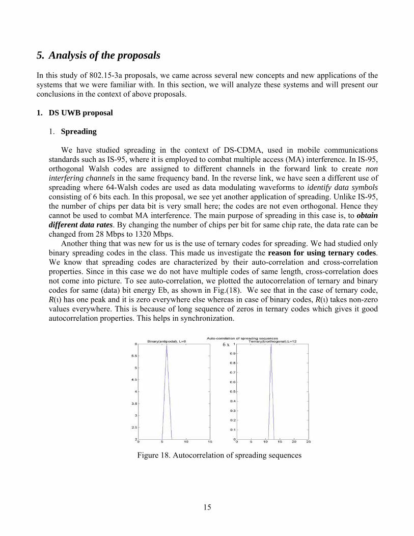
We have studied spreading in the context of DS-CDMA, used in mobile communications standards such as IS-95, where it is employed to combat multiple access (MA) interference. In IS-95, orthogonal Walsh codes are assigned to different channels in the forward link to create non interfering channels in the same frequency band. In the reverse link, we have seen a different use of spreading where 64-Walsh codes are used as data modulating waveforms to identify data symbols consisting of 6 bits each. In this proposal, we see yet another application of spreading. Unlike IS-95, the number of chips per data bit is very small here; the codes are not even orthogonal. Hence they cannot be used to combat MA interference. The main purpose of spreading in this case is, to obtain different data rates. By changing the number of chips per bit for same chip rate, the data rate can be changed from 28 Mbps to 1320 Mbps.

Another thing that was new for us is the use of ternary codes for spreading. We had studied only binary spreading codes in the class. This made us investigate the reason for using ternary codes. We know that spreading codes are characterized by their auto-correlation and cross-correlation properties. Since in this case we do not have multiple codes of same length, cross-correlation does not come into picture. To see auto-correlation, we plotted the autocorrelation of ternary and binary codes for same (data) bit energy Eb, as shown in Fig.(18). We see that in the case of ternary code, R(ι) has one peak and it is zero everywhere else whereas in case of binary codes, R(ι) takes non-zero values everywhere. This is because of long sequence of zeros in ternary codes which gives it good autocorrelation properties. This helps in synchronization.

6 x

Figure 18. Autocorrelation of spreading sequences

16

To further compare binary and ternary codes, we plotted the probability of error vs. Eb/No (Eb energy per bit) for AWGN channel for codes achieving same data rates, as shown in Fig. (21). As can be seen, the performance of binary codes is much better than that of ternary. The reason for this is explained as follows:

Because binary codes are all antipodal, they can be represented by a common structure irrespective of the length of the codes. If E is the energy per coded bit (Energy per bit after convolutional encoding if R=1/2 or the energy per data bit if R=1), then the transmitted waveform after spreading is as shown in figure 19.

+1: a(t) -1: -a(t)

Figure 19 BPSK waveforms and the conditional expected values after demodulation

At the receiver, it is demodulated with the matched waveform having unit energy, as shown on

right. Therefore the decision has to be made from two choices shown on the line above, which is equivalent to hard decision. This is basically equivalent to a BPSK scheme in AWGN with/without convolutional encoding.

In ternary codes, one of 4 possible waveforms is transmitted having the following general property,

0)()()()()()()()( 43234121 ==== ∫∫∫∫ dttatadttatadttatadttata

Edttatadttata −== ∫∫ )()()()( 4231 This is shown in the Figure below:

Figure 20. 4-BOK waveforms and the conditional expected values after demodulation

At the receiver, the demodulating waveform have same shapes as the transmitted ones but with unit energy. Since the transmitted waveforms have equal energy, the optimal decision rule is to correlate the received waveform r(t) with all four waveforms and choose the maximum. This gives rise to the choices as shown on the line in Fig.(20). When the correlating waveform is same as the transmitted one, the correlator output is 1nE + where )2/,0(~ 01 NNn ; when it is of opposite polarity than the

transmitted one, the output is 1nE +− , in both other cases when the correlating waveform is orthogonal to the transmitted one, the output is zero. Thus in this case it is more likely to make errors as the distance between the words at the output of the correlator is much smaller than that in case of

17

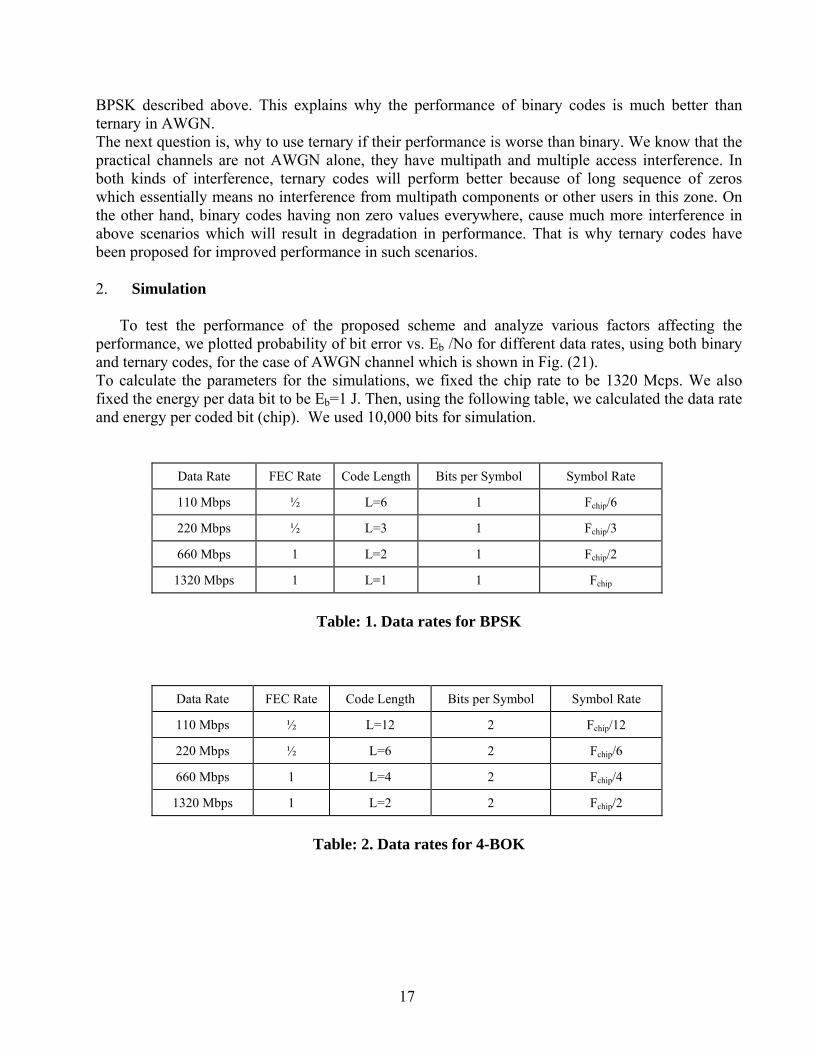
BPSK described above. This explains why the performance of binary codes is much better than ternary in AWGN. The next question is, why to use ternary if their performance is worse than binary. We know that the practical channels are not AWGN alone, they have multipath and multiple access interference. In both kinds of interference, ternary codes will perform better because of long sequence of zeros which essentially means no interference from multipath components or other users in this zone. On the other hand, binary codes having non zero values everywhere, cause much more interference in above scenarios which will result in degradation in performance. That is why ternary codes have been proposed for improved performance in such scenarios. 2. Simulation

To test the performance of the proposed scheme and analyze various factors affecting the performance, we plotted probability of bit error vs. Eb /No for different data rates, using both binary and ternary codes, for the case of AWGN channel which is shown in Fig. (21). To calculate the parameters for the simulations, we fixed the chip rate to be 1320 Mcps. We also fixed the energy per data bit to be Eb=1 J. Then, using the following table, we calculated the data rate and energy per coded bit (chip). We used 10,000 bits for simulation.

Data Rate FEC Rate Code Length Bits per Symbol Symbol Rate

110 Mbps ½ L=6 1 Fchip/6

220 Mbps ½ L=3 1 Fchip/3

660 Mbps 1 L=2 1 Fchip/2

1320 Mbps 1 L=1 1 Fchip

Table: 1. Data rates for BPSK

Data Rate FEC Rate Code Length Bits per Symbol Symbol Rate

110 Mbps ½ L=12 2 Fchip/12

220 Mbps ½ L=6 2 Fchip/6

660 Mbps 1 L=4 2 Fchip/4

1320 Mbps 1 L=2 2 Fchip/2

Table: 2. Data rates for 4-BOK

18

-5 0 5 10 1510-4

10-3

10-2

10-1

100

Pb

Eb/N0 (in dB)

110 Mbps 220 6601320110 Mbps2206601320

BPSK

4-BOK

Figure 21. Probability of bit error vs. Eb /No for different data rates for BPSK and 4-BOK

As can be seen that BPSK performs much better than 4-BOK in AWGN channel, which has been explained earlier. There is almost no difference in the performance of BPSK for data rates 110 & 220 Mbps and similarly for 660 & 1320 Mbps. This is because these schemes are basically BPSK with different modulating waveforms obtained by using different number of chips. We know that the performance of BPSK depends only on the energy and not on the shape of the waveforms, hence for same SNR, we get the same performance in these cases. The difference in the performance at 110 Mbps and 660 Mbps is due to coding. For 110 Mbps, FEC has been used with R=1/2 whereas for 660 Mbps, there is no coding. The crossover point exists because before the crossover the loss in energy per coded bit dominates the gain due to coding and after the intersection point, it is the coding gain which comes into picture.

19

2. MB OFDM proposal

1. Puncturing In MB OFDM proposal, we see a different use of convolutional encoder as we saw of spreading in DS-UWB proposal. Here, the main purpose of a convolutional encoder is to provide different data rates through puncturing, apart from providing forward error correction. By using different puncturing patterns, different output rates can be generated from the convolutional encoder. Because some of the bits are stolen from the encoded data which are not known at the receiver, the receiver inserts dummy zero bits in the demodulated waveform before feeding the data into Viterbi decoder. Because the original bits in these dummy bit positions can be either 1 or 0 with equal probability, it means that about half of the dummy bits do not match with the original bits. This introduces errors in Viterbi decoding. We can see this Fig.(22). For data rates 203.7 Mbps and 673.55 Mbps, the output has rate ½, which is obtained by puncturing 1 bit out of 3 bits from the output of rate 1/3 convolutional encoder. To be specific, the puncturing pattern used is 101. When we compare the performance with puncturing with that without puncturing, we see that in case of puncturing, the error decreases very slowly with increasing Eb/No. This is because of the errors introduced by Viterbi decoder in the absence of the knowledge of the polarity of stolen bits. A second observation here is that the error kind of saturates after a certain Eb/No. As was suggested during the presentation, we checked our programs again to see if the saturation is due to any reason other than puncturing but it turns out that this saturation is due to puncturing only. We observed that the outputs match in all positions but the ones where zero has been inserted (every second bit out of three bits). This means that no error has been introduced by any block till the zero inserting block. The error comes when this output is fed into Viterbi decoder and it seems that the Viterbi decoder is not being able to correct for the inserted dummy bits. As it shows, the error is almost constant for all simulation runs and this error is same as that reached in saturation in Fig.(22). This means that this error is coming because of puncturing. Thus our conclusion is that puncturing can be used to increase data rates but we may have to pay a lot in terms of probability of error if Eb/No is kept same.

2. Interleaving As has been described earlier in the discussion of MB-OFDM proposal, this scheme uses a two stage block interleaver for scrambling the output of the convolutional encoder. One of them uses the block of size 6Ncbps and the other uses the block of size Ncbps. The reason for splitting the interleaver into two stages can be explained as follows: Since the transmitted signal has very wide bandwidth, it can be interfered by both narrowband and wide band interferers. To combat narrowband interference, it is sufficient to scramble the bits over a bandwidth greater than the average bandwidth of a narrowband signal. This is accomplished by scrambling the block of Ncbps bits which are transmitted over a band of 528- MHz. On the other hand, to combat wide band interference, the bits need to be scrambled over a much lager bandwidth. This is accomplished by the interleaving block of 6Ncbps bits. The question is, why not use a single interleaving block of size 6Ncbps which will protect the signal from both narrowband and wideband interference and the answer comes if we consider the complexity of the interleaver. The first stage takes larger blocks of bits and moves them together, so that not all the bits (in original sequence) in the range of wideband interferer go in error. The

20

second block takes smaller blocks of bits and moves them in a smaller range which greatly reduces the complexity compared to if it had to do the same operation over 6Ncbps range. Other thing that we observed is that because of block interleaving, zero padding has to be done in each frame to make the data length fit the interleaver block. This adds to the overhead and is a waste if we compare it with convolutional interleaver, used in DS-UWB, which doesn’t need any zero padding. Also, convolutional interleaver requires less memory than block interleaver. Hence if convolutional interleaver is employed in MB-OFDM, the complexity can be reduced.

3. Modulation For data rates less than 80 Mbps, this proposal duplicates the QPSK modulated signal to make the input to the IFFT block conjugate symmetric. This wastes the energy spent per bit for successful transmission. As we can see from Fig.(22) that to achieve same probability of error, Eb/No required is much higher if conjugate symmetry is used. The performance can be improved though if we use the optimal receiver for this case. In our simulation, we had not used additional information from conjugate symmetry and had simply discarded the additional conjugate bits after taking FFT. However, in an optimal receiver for AWGN, one should minimize the sum of the distance of the received non-conjugate words from codewords in original QPSK constellation and that of received conjugate symmetric words from the conjugate constellation of the above. Still, unless the gain obtained by this optimal receiving strategy overcomes the loss due to decreased energy per coded bit, the use of conjugate symmetry will cost as the degradation in performance.

4. Simulation

To test the performance of the proposed scheme and analyze various factors affecting the performance, we plotted probability of bit error vs. EB /No (EB is the energy per data byte) for different data rates for the case of AWGN channel which is shown in Fig. (22). To calculate the parameters for the simulations, we fixed the duration of OFDM symbol to T=242.42 ns as given in proposal. We also fixed the energy per coded byte to be E = 1/2*T/2 (based on QPSK modulation). If L is the length of input vector in bytes which we fixed to be 10,000, and EB denotes the energy per data byte, then the data rate and energy per byte can be calculated as shown in the table below: Coding rate R

Ncbps N = No.of OFDM symbols

Data rate = L/(T*N) (MBps)

EB = (2*128*N*E)/L (in *10^(-6))

1/3 100 2400 137.5 0.4655 11/32 100 2328 141.5 0.4515 ½ 100 203.7 0.3142 1/3 200 451.28 0.1418 11/32 200 465.24 0.1376 ½ 200 673.55 0.0950

21

-5 0 5 10 15 2010-4

10-3

10-2

10-1

100

Pb

EB/N0 (in dB)

137.5 MBps141.75203.7451.28465.24673.55

Figure 22 Probability of bit error vs. EB /No for different data rates From this plot, it can be observed that as the data rate is increased from 137.5 MBps to 141.75 MBps or 451.28 MBps to 465.24 MBps, the probability of error is slightly increased. This is because the data rate is increased through puncturing, however since only one out of every 33 bits is punctured in these cases, there is only very small performance degradation. On the other hand, for the data rates of 203.7 MBps and 673.55 MBps, one out of every 3 bits has been punctured and that is what results in very poor performance as explained earlier. The difference in blue/red and black/magenta curves is due to the overhead (in terms of energy per bit in channel) paid in duplicating the data bits as explained earlier. Further it should be noted that the SNR and data rates are in terms of energy per byte to noise ratio, and MBps respectively. Hence if these quantities are converted into energy per bit to noise ratio and Mbps, the performance will look much better than it looks in above plot.

22

Conclusion In this project, we studied the DS-UWB and MB-OFDM Physical Layer proposals for 802.15-3a. In both the proposals, UWB signals have been designed using conventional signaling techniques. The aim of both the schemes is to obtain varying data rates for multimedia applications, ranging from moderate to very high, of the order of Gbps, using the spectrum from 3.1 to 10.6 GHz. Varying data rates are obtained by using various techniques at various stages e.g. puncturing, DS spreading, conjugate symmetry and time-frequency coding. It is observed that the in case of lower data rates, bits are much more protected combining several techniques together as mentioned above, which can be used for data transmission requiring high accuracy. For the case of high data rates, the protection is less and hence the probability of error is high, so these can be used for real time communications etc. where little degradation in quality is not as important as fast transmission of data. Through our analysis, we saw that there are various trade offs such as, performance of binary & ternary codes in different channels, increase in data rate through spreading which doesn’t change the probability of error (DS-UWB, BPSK) vs. using puncturing along with convolutional coding, using conjugate symmetry vs. not using conjugate symmetry in OFDM. Thus for actual application, one can choose from various options which gives the best tradeoff between the QOS required and the available combination of techniques. Extra work Apart from the work mentioned above, we have done some other works during our project which may be of interest for somebody willing to work on this topic. When we had started this project, we first built a simulink model for both DS-UWB and MB-OFDM. The blocks were running perfectly except that in DS-UWB, unexpected delays were introduced in using ‘Repeat sequence block’ for spreading, which was varying with increasing simulation time, due to which synchronization became difficult and we couldn’t obtain final results from it. In MB-OFDM block, all the blocks were giving correct output individually and the time offset of each clock had also been set to synchronize all the blocks but when we integrated all the blocks together, it introduced little time shifts at some bits due to which the final output didn’t match the input and we couldn’t calculate probability of error. Hence we had to switch to Matlab programming to obtain our results. We have attached the simulink block diagram at the end so that if somebody wants to use it later, they can debug for the above errors and use the blocks for their analysis. The program for multipath analysis was almost ready, but due to time constraint we couldn’t run the simulations and hance couldn’t include the results in this report. These programs are also attached at the end.

23

BIBLIOGRAPHY 1. IEEE P802.15, Wireless Personal Area Networks: DS-UWB Physical Layer Submission to 802.15 Task Group 3a. and Multiband OFDM Physical Layer Proposal for IEEE 802.15 Task Group 3a. 2. Jeffrey R. Foerster, Marcus Pendergrass and Andreas F. Molisch; ‘A Channel Model for Ultrawideband Indoor Communication’.

3. An Introduction to Multicarrier Modulation, Notes for ECE1520 Data Communications by Teng Joon Lim, Edwards S. Rogers Sr. Dept. of Elect. & Comp. Engineering,University of Toronto 4. Lecture notes, EECS 555 by Prof. W. Stark, University of Michigan.