University of Dundee Adaptive time-stepping for ... · david a. kay†,philipm.gresho‡, david f....

University of Dundee

Adaptive time-stepping for incompressible flow. Part II: Navier-Stokes equations

Kay, David A.; Gresho, Philip M.; Griffiths, David; Silvester, David J.

Published in:SIAM Journal on Scientific Computing

DOI:10.1137/080728032

Publication date:2010

Link to publication in Discovery Research Portal

Citation for published version (APA):Kay, D. A., Gresho, P. M., Griffiths, D., & Silvester, D. J. (2010). Adaptive time-stepping for incompressible flow.Part II: Navier-Stokes equations. SIAM Journal on Scientific Computing, 32(1), 111-128. 10.1137/080728032

General rightsCopyright and moral rights for the publications made accessible in Discovery Research Portal are retained by the authors and/or othercopyright owners and it is a condition of accessing publications that users recognise and abide by the legal requirements associated withthese rights.

• Users may download and print one copy of any publication from Discovery Research Portal for the purpose of private study or research. • You may not further distribute the material or use it for any profit-making activity or commercial gain. • You may freely distribute the URL identifying the publication in the public portal.

Take down policyIf you believe that this document breaches copyright please contact us providing details, and we will remove access to the work immediatelyand investigate your claim.

Download date: 19. Mar. 2016

http://dx.doi.org/10.1137/080728032

http://discovery.dundee.ac.uk/portal/en/research/adaptive-timestepping-for-incompressible-flow-part-ii-navierstokes-equations(422e390a-5ffc-48db-a575-f3e31c8bb3ce).html

SIAM J. SCI. COMPUT. c© 2010 Society for Industrial and Applied MathematicsVol. 32, No. 1, pp. 111–128

ADAPTIVE TIME-STEPPING FOR INCOMPRESSIBLE FLOWPART II: NAVIER–STOKES EQUATIONS∗

DAVID A. KAY† , PHILIP M. GRESHO‡ , DAVID F. GRIFFITHS§ , AND

DAVID J. SILVESTER¶

Abstract. We outline a new class of robust and efficient methods for solving the Navier–Stokes equations. We describe a general solution strategy that has two basic building blocks: animplicit time integrator using a stabilized trapezoid rule with an explicit Adams–Bashforth methodfor error control, and a robust Krylov subspace solver for the spatially discretized system. We presentnumerical experiments illustrating the potential of our approach.

Key words. time-stepping, adaptivity, Navier–Stokes, preconditioning, fast solvers

AMS subject classifications. 65M12, 65M15, 65M20

DOI. 10.1137/080728032

1. Background and context. Simulation of the motion of an incompressiblefluid remains an important but very challenging problem. The resources required foraccurate three-dimensional simulation of practical flows test even the most advanced ofsupercomputer hardware. The effectiveness of our stabilized TR–AB2 time-steppingalgorithm that we explore here is demonstrated in the context of convection-diffusionproblems in part I of this work [8]. Therein it is shown that stabilized TR–AB2is particularly well suited to long time integration of advection-dominated problemsand is a very effective algorithm when faced with general advection-diffusion problemswith different time scales governing the system evolution. In this paper, our focus ison assessing the performance of the integrator in combination with a state-of-the-artiterative solver in the context of method-of-lines discretization of the Navier–Stokesequations.

For simplicity, the case of a two-dimensional flow domain Ω is considered here.Our solver methodology is exactly the same in the case of a three-dimensional flowmodel. Thus, the flow domain boundary Γ consists of two nonoverlapping segmentsΓD ∪ ΓN associated with specified flow and natural outflow boundary conditions,respectively,

∂�u

∂t− ν∇2�u+ �u · ∇�u+∇p = 0 in Ω× [0, T ],(1.1)

−∇ · �u = 0 in Ω× [0, T ],(1.2)

∗Received by the editors June 21, 2008; accepted for publication (in revised form) February 9,2009; published electronically February 5, 2010. This collaboration was supported by EPSRC grantGR/R26092/1.

http://www.siam.org/journals/sisc/32-1/72803.html†Oxford University Computing Laboratory, Oxford, OX1 3QD, UK ([email protected]).‡Livermore, CA ([email protected]).§Division of Mathematics, University of Dundee, Dundee, DD1 4HN, Scotland, UK (dfg@maths.

dundee.ac.uk).¶School of Mathematics, University of Manchester, Manchester, M13 9PL, UK (d.silvester@

manchester.ac.uk).

111

112 D. KAY, P. GRESHO, D. GRIFFITHS, AND D. SILVESTER

�u = �g on ΓD × [0, T ],(1.3)

ν∇�u · �n− p�n = �0 on ΓN × [0, T ],(1.4)

�u(�x, 0) = �u0(�x) in Ω.(1.5)

Our notation is completely standard: �u is the fluid velocity, p is the scalar pressure,ν > 0 is a specified viscosity parameter (in a nondimensional setting it is the inverseof the Reynolds number), and T > 0 is some final time. The initial velocity field �u0is typically assumed to satisfy the incompressibility constraint, that is, ∇ · �u0 = 0.Unless stated otherwise, it is implicitly assumed that ΓN has nonzero measure, inwhich case the pressure p is uniquely specified by the outflow boundary condition.

Conventional approaches to solving the initial value problem (1.1)–(1.5) typicallyuse semi-implicit time integration leading to a Poisson or Stokes-type problem at ev-ery time step, but with a stability restriction on the time step. In contrast, there isno time-step restriction in our case. The price that must be paid for this improvedrobustness is the need to solve a so-called Oseen problem at every time step. For-tunately, very efficient solvers for Oseen problems have become a reality in the lastdecade; see, for example, [6], [13], [3], [2]. Specifically, the preconditioning frame-work that has evolved offers the possibility of uniformly fast convergence independentof the problem parameters (namely, the mesh size, the time step, and the Reynoldsnumber).

A common viewpoint (see, for example, Turek [18]) is that a coupled solver ismainly of use for steady flows, whereas projection-type schemes are preferred whenmodeling unsteady flows. We aim to challenge this assertion. Of course, projection-type schemes can be very effective—especially if implemented using multigrid andcombined with a fixed time-stepping strategy. Their limitation is the fact that decou-pling the velocity and pressure inevitably leads to smaller time steps when comparedto a coupled solver strategy. The big attraction of an implicit discretization in timeis that it enables the possibility of self-adaptive time-step control, with time stepsautomatically chosen to “follow the physics.”

An outline of the paper is as follows. The temporal and spatial discretizationof (1.1)–(1.5) is discussed in section 2. The linear algebra aspects are discussed insection 3, and the performance of our solver methodology is assessed in section 4.We have tested our solver on a range of flow problems. Results for two benchmarkflow problems are presented here: first, a driven cavity flow that ultimately reaches asteady state; and second, a developing flow around a cylinder that reaches a periodicstate of vortex shedding. We hope that, at the end, the reader will be convincednot only that incompressible flow problems can be solved more efficiently using anadaptive time integrator but also that studying the behavior of the computed timestep can help to delineate different phases of the evolution of the flow.

2. Discretization aspects. Our “basic” time-stepping algorithm is the well-known, second-order accurate, trapezoid rule (TR). Let the interval [0, T ] be dividedinto N steps, {ti}Ni=1, and let �vj denote �v(�x, tj). The semidiscretized problem is the

following: Given (�un, pn) at time level tn and boundary data �gn+1 at time level tn+1,

ADAPTIVE TIME-STEPPING 113

compute (�un+1, pn+1) via1

2

kn+1�un+1 − ν∇2�un+1 + �un+1 · ∇�un+1 +∇pn+1 =

2

kn+1�un +

∂�u

∂t

n

in Ω,(2.1)

−∇ · �un+1 = 0 in Ω,(2.2)

�un+1 = �gn+1 on ΓD,(2.3)

ν∇�un+1 · �n− pn+1�n = �0 on ΓN .(2.4)

Here, kn+1 := tn+1−tn is the current time step, and ∂�u∂t

n:= ν∇2�un−�un ·∇�un−∇pn

is shorthand for the acceleration at time tn.The limited stability of TR time-stepping for the incompressible Navier–Stokes

equations is extensively discussed in the literature, for example, in the well-cited paperby Simo and Armero [15]. The basic algorithm has some attractive features, however.In particular, solving a simple ODE model of convection-diffusion,

y = −(1

τ+ iω

)y, y(0) = 1,(2.5)

where τ corresponds to a decay time constant and ω is a frequency parameter, itis easily shown (see [8, sect. 2]) that TR is unconditionally stable (A-stable) andnondissipative. This is important when modeling pure advection (τ = ∞), or evenadvection-dominated problems ( 1τ � ω). Dettmer and Peric [1] critically compare TRwith alternative time-stepping algorithms in the context of fixed time-step algorithmsfor convection-diffusion equations and for Navier–Stokes equations. They presentresults showing that the lack of numerical damping within TR can be problematicif the time step is kept fixed (and is not small enough). Smith and Silvester [14]draw similar conclusions when comparing fixed time-step TR with the three-stageoperator-splitting methods advocated by Turek [18]. Such problems are circumventedif an adaptive time-step strategy is employed and the TR method is stabilized asdescribed later.

From (2.1) it is evident that a numerical scheme for handling the nonlinear term�un+1 · ∇�un+1 is needed at every time step. A standard approach (see Gresho andSani [9, p. 800]) would be solve the system (2.1)–(2.4) to a predefined accuracy usingsome variant of the Newton iteration. Although this requires inner iterations, theapproach may still be cost-effective if it avoids any loss of stability which, using self-adaptive time-stepping, usually leads to a reduction in the time-step size. We advocatean alternative approach in this work—computational experiments in the final sectionshow that if the linearization is done using �un+1 · ∇�un+1 ≈ �wn+1 · ∇�un+1, where

(2.6) �wn+1 = (1 + (kn+1/kn))�un − (kn+1/kn)�u

n−1,

then temporal stability is not compromised significantly. The linearization (2.6) isthus adopted in the remainder of the paper. In the case of constant time-stepping,our methodology is essentially the same as the approach of Simo and Armero [15] andthe TRLE algorithm described in [10, p. 163].

1This is the usual implementation of TR; see Gresho and Sani [9, p. 797]. An alternative interpre-tation (see Layton [10, p. 163]) is that an implicit midpoint evaluation of the the quadratic convection

term �un+1/2 · ∇�un+1/2 is computed via the second order update (�un+1 · ∇�un+1 + �un · ∇�un)/2.


Let (·, ·) denote the standard scalar or vector valued L2 inner product definedon Ω. Given the velocity solution space H1

�g = {�v|�v ∈ H1(Ω)2; �v|ΓD = �g}, thelinearized semidiscrete problem can be formulated as a variational problem: given(�un, pn) ∈ H1

�gn × L2(Ω), we seek (�un+1, pn+1) ∈ H1�gn+1 × L2(Ω) such that

2

kn+1(�un+1, �v) + ν (∇�un+1,∇�v) + (�wn+1 · ∇�un+1, �v)− (pn+1,∇ · �v)

=2

kn+1(�un, �v) +

(∂�u

∂t

n

, �v

),(2.7)

(∇ · �un+1, q) = 0(2.8)

for all (�v, q) ∈ H1�0(Ω)× L2(Ω).

Throughout this paper, spatial discretization will be done using a method-of-lines approach based on finite element approximation on a fixed spatial grid. Ouralgorithm methodology described below thus applies essentially verbatim to finitedifference and finite volume discretizations. The domain Ω is split into finitely manynonoverlapping triangles τ , giving a triangulation Th. (The mesh parameter h canbe associated with the length of the longest edge of a triangle from Th.) Low-ordermixed approximation methods are not stable2 in general. One mixed method that isstable is the so-called Taylor–Hood P2–P1 method, which uses continuous piecewisequadratic approximation for the velocity components and continuous piecewise linearapproximation for pressure. We use Taylor–Hood approximation throughout this workbut emphasize that the rapid convergence properties of the linear solver methodologydescribed in the next section are essentially independent of the mixed approximationused.

Thus, using finite-dimensional approximation spaces X ⊂ H1�0and M ⊂ L2(Ω),

the fully discrete problem is to find (�un+1h , pn+1

h ) ∈ X�g ×M such that

2

kn+1(�un+1

h , �vh) + ν (∇�un+1h ,∇�vh) + (�wn+1

h · ∇�un+1h , �vh)− (pn+1

h ,∇ · �vh)

=2

kn+1(�unh, �vh) +

(∂�uh∂t

n

, �vh

),(2.9)

(∇ · �un+1h , qh) = 0(2.10)

for all (�vh, qh) ∈ X ×M . The linear algebra version of (2.9)–(2.10) will be explicitlyconstructed in the next section.

Our adaptive time-stepping algorithm is a refined version of the “smart integra-tor” advocated by Gresho and Sani [9, sect. 3.16.4] and has three ingredients: timeintegration, the time-step selection method, and stabilization of the integrator. Webriefly discuss each of these separately below so as to mirror the discussion in part I;see [8, sect. 1].

Time integration. We are conscious of the need to minimize potential round-offinstability; thus our implementation of the TR–AB2 pair explicitly computes the dis-crete velocity updates scaled by the time step to avoid underflow and inhibit subtrac-

tive cancellation. Specifically, given �unh,∂un

h

∂t , and the boundary update �g := �gn+1−�gn

kn+1,

2See Elman, Silvester, and Wathen [5, Ch. 5] for a full discussion of inf-sup stability.


we first compute the pair (�dn

h , pn+1h ) ∈ X�g ×M such that

2(�dn

h, �vh) + νkn+1 (∇�dn

h,∇�vh) + kn+1(�wn+1h · ∇�d

n

h, �vh)− (pn+1h ,∇ · �vh)

=

(∂�unh∂t

, �vh

)− ν (∇�unh,∇�vh)− (�wn+1

h · ∇�unh, �vh),(2.11)

(∇ · �dn+1

h , qh) = 0(2.12)

for all (�vh, qh) ∈ X×M , and then we update the TR velocity field and the acceleration(time derivative of the velocity) via

(2.13) �un+1h = �unh + kn+1

�dn

h;∂�un+1

h

∂t= 2�d

n

h − ∂�unh∂t

.

We will subsequently refer to (2.11)–(2.12) as the discrete Oseen problem. Note thatthe computed pressure field pn+1

h is not needed for subsequent time steps and doesnot play a role in the time-step selection process described next.

Time-step selection. To control the time integration it is usual to place a user-specified tolerance, ε, on the L2 norm of the truncation error at the next time step,�en+1h , so that

(2.14) ‖�en+1h ‖ ≤ ε‖�u∞h ‖,

where ‖�u∞h ‖ is (a possibly user-specified estimate of) the maximum norm of themethod-of-lines solution over the prescribed time interval.3 Assuming that the un-derlying ODE system has smooth third derivatives in time (so that the TR timeintegration is indeed second-order accurate) standard manipulation of Taylor seriesshows that the ratio of successive truncation errors is proportional to the cube ofthe ratio of successive time steps. This motivates the following time-step selectionheuristic:

(2.15) kn+2 = kn+1

(ε/‖�en+1

h ‖) 1

3

.

The local truncation error �en+1h is estimated by comparing the TR velocity solution

�un+1h with the AB2 velocity solution �un+1

∗ computed using the explicit update formula

(2.16) �un+1∗ = �unh +

kn+1

2

[(2 +

kn+1

kn

)∂unh∂t

−(kn+1

kn

)∂�un−1

h

∂t

],

using the standard estimate (cf. part I, [8, p. 2021])

(2.17) �en+1h = (�un+1

h − �un+1∗ )/[3(1 + kn/kn+1)].

To implement this methodology in a practical code there are two start-up issuesthat need to be addressed:

1. AB2 is not self-starting. To start the simulation we require a finite elementfunction �u0h with boundary data �g0 that satisfies the discrete incompressibil-ity constraint

(2.18) (∇ · �u0h, qh) = 0 for all qh ∈M.

3‖�u∞h ‖ = 1 in all of the examples discussed in this paper.


The initial acceleration (and concomitant pressure) is then computed bysolving the discrete (potential flow) problem: given the boundary update

�g := �g1−�g0

k1, we compute the pair (

∂�u0h

∂t , p0h) ∈ X�g ×M such that

(∂�u0h∂t

, �vh

)− (p0h,∇ · �vh) = −ν (∇�u0,∇�v)− (�u0 · ∇�u0, �v),(2.19)

(∇ · ∂�u

0h

∂t, qh

)= 0(2.20)

for all (�vh, qh) ∈ X ×M . We then set n = 0 and define �w1h = �u0h + k1

∂�u0h

∂t soas to construct the discrete Oseen problem (2.9)–(2.10). Solving this discreteOseen problem gives (�u1h, p

1h) (the TR velocity and pressure) at the end of

the first time step. The acceleration at time t = k1 is then computed using∂�u1

h

∂t = 2k1(�u1h − �u0h)−

∂�u0h

∂t and allows us to compute the AB2 velocity at thesecond time step. To complete the start-up process, time step control is thenswitched on at the third time step (k1 = k0).

2. Choice of initial time step k0. Several strategies are available with which tostart the TR method. Our strategy is to select a conservatively small value fork0 (say, 10−8). With such a choice we will have rapid growth in the time step:typically ‖�enh‖ = O(eps) for the first few time steps (where eps is machineprecision), and so kn+1/kn = O((ε/eps)1/3) ≈ 104 when ε = 10−4. Thisrapid growth implies that, for small values of n, we see exponential growthin the time step, and with very few such steps (typically 2–4) a time step isobtained that is commensurate with the “initial response time.” See part I [8,p. 2021] for further discussion of this point.

A general purpose ODE code in a software library will typically have multiplebells and whistles. In contrast, our time-stepping algorithm has just one “trip”:

1. Time-step rejection. After computing the new time step via (2.15), we checkto see if the next step is seriously reduced,4 i.e., kn+2 < 0.7kn+1, or equiva-lently that ‖�en+1

h ‖ > (1/0.7)3ε. If this happens, then the next time step isrejected: the value of kn+1 is multiplied by (ε/‖�en+1

h ‖)1/3, and the currentstep is repeated with this smaller value of kn+1.

Stabilization of the integrator. As discussed earlier, the TR method is prone to“ringing” when solving stiff problems (typically for PDEs when using very small spa-tial grid sizes to resolve fine detail) with relatively large tolerances on the time stepor toward the end of a simulation when close to steady state. Situations such asthese are discussed by Osterby [11] along with a variety of means of suppressing theoscillations. Our code implements an alternative strategy—time-step averaging. Theaveraging is invoked periodically every n∗ steps. For such a step, we save the values

t∗ = tn and �u∗h = �unh, and, having computed the TR update �dn

h via (2.11)–(2.12),we set tn = tn−1 +

12kn and tn+1 = t∗ + 1

2kn+1 and define the new “shifted” solution

4For example, if the iterative solver discussed in section 3 does not solve the discrete Oseenproblem to the required accuracy, then ‖�enh‖ will be larger than we would expect for the currenttime step. If the step is repeated with a smaller step size, then the associated linear algebra problemis more easily solved so the time-stepping algorithm can recover.


Fig. 1. Stabilized TR–AB2 integrator with periodic averaging: log kj versus time-step numberj for a driven cavity flow with viscosity ν = 1/100 being spun up from rest.

vectors so that

�unh =1

2(�u∗h + �un−1

h ),∂�unh∂t

=1

2

(∂�unh∂t

+∂�un−1

h

∂t

),(2.21)

�un+1h = �u∗h + 1

2kn+1�dn

h ,∂�un+1

h

∂t= �d

n

h .(2.22)

We then compute the next time step using (2.15) and continue the integration. Theaveraging process annihilates any contribution of the form (−1)n to the solution andits time derivative, thus cutting short the “ringing” while maintaining second-orderaccuracy. In our code the parameter n∗ is a fixed parameter—typically 10. (A wayof calculating a suitable value n∗ on the fly is discussed in part I [8, p. 2023].) Thebenefit of this simple stabilization strategy is illustrated in Figure 1, which shows thebehavior of stabilized and unstabilized TR–AB2 for a driven cavity flow problem for aReynolds number Re = UL/ν = 100. The fluid is initially at rest, and the tangentialvelocity of one of the boundaries is smoothly increased to a value of unity; full detailsare discussed later. Since the underlying Reynolds number is small enough, the flowsolution tends to a steady state as t→ ∞.

Looking at Figure 1, we see that the unstabilized TR–AB2 integrator generatesa constant time step as the steady state is approached. This behavior is erroneous inthe sense that if we were to follow the physics, then the time step would increase aswe approach the steady state. This is what we see when we stabilize the integrator,and it is independent of the frequency of averaging. Note that there is a drop-off inperformance when we average too frequently or too infrequently—our default choiceof n∗ = 10 is essentially a compromise between enforcing stability and maintainingaccuracy. This is the value of n∗ that was used when generating the results presentedin section 4.


3. Solving the discrete Oseen system. Let {φi}nu

i=1 define the basis set forthe approximation of a function from the space H1

0 := {v|v ∈ H1(Ω); v|ΓD = 0},and let {ψj}np

j=1 define a basis set for the discrete pressure. The fully discrete solu-

tion (�un+1h , pn+1

h ) corresponding to the Oseen problem (2.9)–(2.10) is given by theexpansions

(3.1) �un+1h =

[ nu∑i=1

αx,n+1i φi,

nu∑i=1

αy,n+1i φi

]+ �gn+1, pn+1

h =

np∑k=1

αp,n+1k ψk,

where αx,n+1, αy,n+1, and αp,n+1 represent vectors of coefficients. These are com-puted by solving the linear equation system defined below.

Given the velocity basis set, we define so-called velocity matrices Mv, Av, andNv, representing identity, diffusion, and convection operators in the velocity space,respectively:

Mv = [Mv]ij = (φi, φj),(3.2)

Av = [Av]ij = (∇φi,∇φj),(3.3)

Nv(�uh) = [Nv]ij = (�uh · ∇φi, φj).(3.4)

Combining the three velocity matrices and using the linearization in (2.7) defines thevelocity convection-diffusion matrix at time tn+1:

(3.5) Fn+1v :=

1

kn+1Mv + νAv +Nv(�w

n+1h ),

with �wn+1h = (1 + (kn+1/kn))�u

nh − (kn+1/kn)�u

n−1h . In addition, given the pressure

basis set, we can define a discrete divergence matrix B = [Bx, By] via

Bx = [Bx]ki = −(ψk,

∂φi∂x

),(3.6)

By = [By]ki = −(ψk,

∂φi∂y

).(3.7)

Looking ahead to preconditioning the discrete system, we also define pressure ma-trix analogues of Mv, Av, and Nv, representing identity, diffusion, and convectionoperators in the pressure space:

Mp = [Mp]k� = (ψk, ψ�),(3.8)

Ap = [Ap]k� = (∇ψk,∇ψ�),(3.9)

Np(�wh) = [Np]k� = (�wh · ∇ψk, ψ�).(3.10)

Finally, using the definitions (3.1)–(3.7), the discretized Oseen problem can beexpressed as the following system: find [αx,n+1,αy,n+1,αp,n+1] ∈ R

nu×nu×np suchthat ⎡

⎣ Fn+1v 0 BT

x

0 Fn+1v BT

y

Bx By 0

⎤⎦⎡⎣ αx,n+1

αy,n+1

αp,n+1

⎤⎦ =

⎡⎣ f x,n+1

f y,n+1

f p,n+1

⎤⎦ .(3.11)

The right-hand-side vector f is constructed from the boundary data �gn+1, the com-

puted velocity �unh at the previous time level, and the acceleration∂�un

h

∂t .


The coefficient matrix in (3.11) may be written in the equivalent form

K :=

[Fn+1

v BT

B 0

],(3.12)

where Fn+1v is a 2 × 2 block diagonal matrix, with diagonal blocks Fn+1

v defined asin (3.5). Thus, at every time level, we are faced with the task of solving a squarenonsingular linear equation system Kα = f. This is done using a (right-) precon-ditioned Krylov subspace method. Such methods start with some guess α0, withresidual r0 = f −Kα0; given a preconditioner, P , say, to be defined later, constructa sequence of approximate solutions of the form

(3.13) αk = α0 + pk,

where pk is a vector in the k-dimensional Krylov space

(3.14) Kk(r0,KP−1) = span{r0,KP−1r0, . . . , (KP

−1)k−1r0} .

The preconditioned GMRES method is used herein. A feature of GMRES is thatit is an optimal Krylov solver in that it computes the unique iterate of the form(3.13) for which the Euclidean (or root mean square) norm of the residual vector issmallest—the classical convergence estimate is

‖rk‖2 = minφk(0)=1

‖φk(KP−1)r0‖2,

where φk is the set of polynomials of degree k. Step m of the process requires onematrix-vector product together with a set of m vector operations, making its cost, interms of both operation counts and storage, proportional to mn, where n = 2nu +np

is the dimension of the system (3.11). A full discussion of GMRES convergenceproperties can be found in [5, Ch. 4], together with details of the construction ofsuccessive GMRES iterates.

At every time level, we set the initial vector α0 = 0 and run the preconditionedGMRES process until either a fixed number of iterations (maxit) is reached, or elsethe stopping-test

‖f−Kαm‖2‖r0‖2

< itol

is satisfied. We denote the solver strategy by GMRES(maxit, itol). Typically, weset maxit to 50, and itol to 10−6. The big task is to construct a preconditioner Psuch that the stopping-test is satisfied for smallm. Furthermore, we would like this mto be independent of the discretization parameter h and the viscosity ν. Given that acomplete description of our preconditioning methodology is given in [13] and [5, Ch.8], we simply outline the key features here.

The general form of an ideal preconditioner is

P =

(Fn+1

v BT

0 −X

),(3.15)

where the np × np matrix X is an approximation to the pressure Schur complementmatrix S = B(Fn+1

v )−1BT . We note that if the exact Schur complement X := S wereused in (3.15), then GMRES would give the exact solution in two iterations, that is,


α2 = α; see Murphy, Golub, and Wathen [7]. Since the Schur complement matrixS is dense, then an equally effective yet relatively inexpensive approximation to it isneeded if this approach is to be practical. Such an approximation is that developed byKay, Loghin, and Wathen [6] and is referred to herein as pressure convection-diffusionpreconditioning. It is given by setting X = Ap(F

n+1p )−1Mp, with the pressure matrix

operators Ap and Mp given in (3.9) and (3.8), respectively, and

(3.16) Fn+1p =

1

kn+1Mp + νAp +Np(�w

n+1h ),

defining the pressure space analogue of the Fn+1v operator in (3.5). The properties of

this Schur complement approximation are the subject of ongoing analysis; see [3] forsome theoretical results in the steady-state case. Numerical experiments showing thegood performance of this preconditioning strategy in the context of steady-state flowproblems are given in [16] and [2].

Note that preconditioning with P requires the action of the inverse of Fn+1v and

X at each GMRES iteration:

P−1 =

((Fn+1

v )−1 (Fn+1v )−1BTX−1

0 −X−1

).(3.17)

Using the pressure convection-diffusion approximation to X , we see that

(3.18) X−1 =M−1p (Fn+1

p )A−1p ,

and thus preconditioning is done by effecting the action of the inverse operators(Fn+1

v )−1, A−1p , and M−1

p . In practice, these matrix operations can be done very effi-ciently using algebraic multigrid (AMG). More specifically, all the results in the nextsection are computed using an inexact preconditioner where the actions of (Fn+1

v )−1

and A−1p are approximated by two AMG V-cycles and the action of the inverse mass

matrix M−1p is approximated by five iterations of a diagonally scaled conjugate gra-

dient algorithm.5

The AMG code that we use for this is a MATLAB version of the subroutineHSL MI20 [4]. It should be stressed that we use this subroutine as a black-box—wespecify three (point Gauss–Seidel) smoothing sweeps (no special reordering) at eachlevel, and all AMG coarsening parameters are set to the default values. The realiza-tion that we were able to generate results without having to incorporate streamlinediffusion into the preconditioner was a big surprise for us.6 The fact that we are usingstandard Galerkin approximation without “tuning parameters” makes for a very cleandiscretization and, in our opinion, makes our methodology look very attractive.

4. Numerical results. The first model problem is the classical lid-driven cavity.The motivation for considering this is to demonstrate the effectiveness of our solverwhen it is used to time step to a steady state. The second model problem is anotherwell-studied problem, namely, that of a channel flow with a cylindrical obstruction.The version of the model that we consider is that proposed by Dettmer and Peric in[1]. An alternative problem statement and a benchmark solution is given by Turek [17,Ch. 1]. The motivation for studying this problem is to show that our solver can be

5Diagonally scaling the mass matrix gives a perfectly conditioned operator; see [5, Lemma 6.3].6The mass matrix contribution coming from the time-stepping is the crucial ingredient here—as

the temporal error tolerance is reduced, the effectiveness of the AMG solver is increased.


used to “follow the physics” of a transition of a flow from a state of rest to a periodicstate of vortex shedding. For a related and detailed analysis of the start-up flow pasta cylinder, see Gresho and Sani [9, Sec. 3.19].

Example 4.1. Consider a spatially discretized system (2.7)–(2.8) defined on aunit square cavity domain. The initial condition is �u0(�x) = 0 in the cavity, and anenclosed flow boundary condition �g = �0 is imposed on three of the walls togetherwith a time-dependent velocity �g = (1− e−5t, 0) on the top boundary 0 < x < 1; y =1. This models a slow start-up from rest. For sufficiently small Reynolds numberRe = 1/ν < 13, 000 the flow tends to a steady state. This consists of a clockwiserotating primary flow, secondary recirculation regions in the two bottom corners, anda tertiary recirculation on the left-hand wall; see Shankar and Deshpande [12]. Forlarger values of the Reynolds number the steady flow is not stable. At a very largeReynolds number the flow will be chaotic and turbulent.

Fig. 2. Stabilized TR–AB2 integrator with periodic averaging for Example 4.1 with viscosityν = 1/1000: log kj versus time step number j. Top: Entire evolution. Bottom: Zoom showing thealmost perfect agreement over the final 20 time steps.

Figure 2 shows the evolution of the time step when we run our solver for aproblem with ν = 1/1000 with time-stepping tolerance ε = 10−4. For simplicity, weuse a uniform mesh of right-angled triangles with edge length h, and we compare thebehavior on two meshes—a basic mesh (red curve) with 1/h = 64 and a refined mesh(blue curve) with 1/h = 128. The time integration was run to a final time of 100 timeunits. Using either mesh, the time step grows monotonically with time and ultimatelyreaches a value of O(10) time units. The time-step evolution can also be seen to beessentially independent of the spatial subdivision—this suggests that the simulationsare time-accurate. The time-step behavior can also be seen to be consistent with thatin Figure 1 with n∗ = 10, which is for an order of magnitude larger viscosity.

The performance of the preconditioned GMRES(50, 10−6) solver is plotted inFigure 3. We observe that the discrete Oseen system becomes progressively moredifficult to solve as the time step grows. On a positive note, however, we also see


Fig. 3. Stabilized TR–AB2 integrator with periodic averaging for Example 4.1 with viscosityν = 1/1000: Number of GMRES iterations versus time step number j.

that the solver performance at each time step is completely insensitive to the meshrefinement level!

Example 4.2. Consider a spatially discretized system (2.7)–(2.8) defined on arectangular domain −5 < x < 16,−4.6 < y < 4.5 with a cylindrical obstruction ofdiameter unity centered at the point (0, 0). The initial condition is �u0(�x) = 0 inthe domain, and a zero flow boundary condition is imposed on the cylinder boundarytogether with a time-dependent velocity �g = (1 − e−5t, 0) on the left-hand (inflow)boundary, as well as at the top and the bottom of the channel. The right-handboundary x = 16,−4.6 < y < 4.5 satisfies the natural outflow condition (1.4) forall time. For a viscosity coefficient in the range 1/1000 ≤ ν ≤ 1/100 the flow tendsto a time periodic vortex shedding solution which subjects the cylinder to oscillatinglift and drag forces acting parallel and perpendicular to the direction of the flow,respectively.

The results in Figure 4 illustrate what happens when we run our solver on theproblem with ν = 1/100, using the relatively coarse mesh shown in Figure 5, withthe time-stepping tolerance ε = 10−4. The top plot shows a snapshot of the flowsolution during the shedding cycle. Also shown is the evolution of the lift coefficientfrom the rest state, and the cyclic variation of the drag coefficient after shedding hasbeen established. With this accuracy tolerance the algorithm generates a constanttime step of 0.05 once in the shedding regime—this corresponds to approximately 100sample points per shedding cycle. Looking at the time-step evolution in Figure 4, wecan identify four distinct phases. First, we have a “fake” initial transient which lasts1–5 time units and which is associated with the dynamic boundary condition. Notethat there is a noticeable “judder” at about 5 time units—roughly speaking when theinitial influx hits the cylinder. Between 5 and 35 time units the integrator runs witha constant time step of about 0.13, corresponding to the lengthening of the pair ofrecirculating eddies in the wake of the cylinder. Finally, after approximately 35 timeunits, stability is lost, the flow symmetry is broken, and the time step automaticallycuts back, ultimately settling on the constant value that is appropriate for the accuratecomputation of the vortex shedding.


Fig. 4. Solution data for Example 4.2 for ν = 1/100 with accuracy ε = 10−4. The y-axis limitsfor the time step in the second plot range from 0 to 0.2, and those for the drag coefficients in thethird plot range from 1.43 to 1.46.

In the remainder of the paper we will critically assess the performance of oursolver, first when run with ν = 1/100, and second when run with ν = 1/400. Ourresults can then be directly compared with those in [1, pp. 1213–1221], where the sameproblems are solved using fixed time-stepping, together with fully implicit approxima-tion (that is, solving nonlinear equations using Newton iteration at each time level).We solve both of these flow problems on three meshes. The coarsest mesh, so-calledlevel 1, is illustrated in Figure 5. It contains 999 triangles and has nu = 2055 velocitydegrees of freedom. An intermediate mesh, so-called level 2, is obtained by a uni-form refinement of the coarsest mesh and contains 3996 triangles and has nu = 8106velocity degrees of freedom. Note that the newly introduced nodes are “moved” tothe cylinder boundary to give a better resolution of the circular geometry. The finestmesh, so-called level 3, is obtained by a uniform refinement of the intermediate mesh,but this time excluding the two regions at the top and the bottom that adjoin the


Fig. 5. Reference mesh for Example 4.2.

inflow in Figure 5. This gives a mesh of 12728 triangles with nu = 25101 velocitydegrees of freedom.

We consider the easier case of ν = 1/100 first. In Figure 6 we present a comparisonplot showing the evolution of the lift coefficient with different mesh refinement levels.We note that the results computed on the level 2 and level 3 meshes are essentiallyindistinguishable from one another. Note that the frequency of shedding is a majorpoint of physical interest. When we compare these results with the lift coefficientevolution computed using a fully implicit second-order time-stepping method that isgiven in [1, Fig. 15], we find very a close match—the frequency of shedding and theamplitude of the lift coefficient are identical in the eyeball norm.

The evolution of the associated time step is also shown in Figure 6. We notefirst that, independent of the spatial refinement, the character of the time-step evo-lution shows the four distinct phases exhibited in Figure 4. We can also see that theconstant time step that is used in the second phase (the development of the recircu-lation zones in the cylinder wake) is mesh-dependent. The fact that the time stepthat is used in the shedding phase is essentially mesh-independent (certainly on thetwo finer levels) confirms that the integrator is time-accurate in this regime. Alsoshown in Figure 6 is the comparison of the iterative solver performance for the threerefinement levels. From this, we see that our preconditioning strategy is extremelyefficient—typically taking 23 GMRES iterations per time step in the shedding phaseon the intermediate mesh and 29 GMRES iterations per time step on the most refinedmesh. We can also see that the algorithm is robust (in the sense that there are fewrejected steps) in the “tough” phases when the solver fails to converge to the accuracytolerance in maxit iterations—for example, during the second phase of the flow evo-lution when using the most refined mesh. Our interpretation of this situation is thatthe time step that is generated by the crude ε = 10−4 tolerance is probably overlyoptimistic during the second phase of the flow evolution. This reduces the effective-ness of the algebraic multigrid preconditioner7 for the velocity convection-diffusionoperator (Fn+1

v )−1. Evidence for this comes from solving the same problem on theintermediate mesh with a tighter error tolerance of ε = 10−7. This generates a smoothhump-shaped time-step evolution with a maximum time step of 0.03 at about 17.5time units and gives constant time steps in the shedding phase which are an order

7We would get much better robustness if we followed the recipe in [5, p. 361] and added astreamline diffusion stabilization term to the discrete operator prior to the set-up phase of the AMGsolver.


Fig. 6. Top: Lift coefficient evolution for Example 4.2 for ν = 1/100 with accuracy ε = 10−4.Bottom: Time step size and number of GMRES iterations versus time step.

of magnitude smaller than those in Figure 6. In this case, the linear solver has noproblem at all—GMRES always satisfies the itol=10−6 residual tolerance criterionin fewer than 25 iterations.

In these experiments the accuracy of the linearized TR–AB2 algorithm is almostidentical to a fully implicit version of the TR–AB2 algorithm. To give a specific exam-ple, the shedding computation on the intermediate mesh was recomputed using a fullyimplicit version of TR. Thus, at every time step we iterated the Oseen solve (2.11)–(2.12) with a simple fixed point (Picard) iteration. The initial approximation for theconvective velocity (�wn+1

h )(0) was given by �unh. At the kth step we set up the system(2.11)–(2.12) with a convection field (�wn+1

h )(k) and solved it using preconditionedGMRES to an accuracy of itol=10−6 to get the solution (dn+1

h )(k). This in turn

gives the updated velocity approximation (�wn+1h )(k+1) := (wn+1

h )(k) + kn+1(dn+1h )(k).

Our fixed point iteration process was terminated when the norm of the differencebetween successive velocity iterates was less than 10−3. Typically, this led to two or


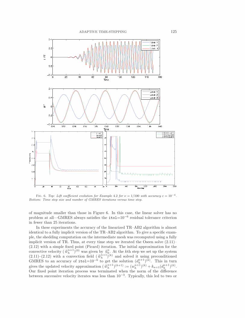
three Picard iterations at every time step. The time step sequence that resulted usingthis nonlinear approach turned out to be almost identical to that generated by our lin-earized method. The complete history and a zoom in the shedding regime are shownin Figure 7. Regarding the relative accuracy of the corresponding flow solutions, theshedding frequencies are essentially identical, and the amplitude of the lift coefficientis slightly bigger, i.e., more accurate, in the nonlinear case. The total computationtime was almost exactly three times longer in the nonlinear case, however!

Fig. 7. Top: Linearized versus nonlinear time stepping for Example 4.2 for ν = 1/100 withaccuracy ε = 10−4. Bottom: Zoom of the time step size versus time in the shedding regime.

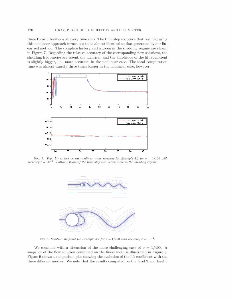
Fig. 8. Solution snapshot for Example 4.2 for ν = 1/400 with accuracy ε = 10−4.

We conclude with a discussion of the more challenging case of ν = 1/400. Asnapshot of the flow solution computed on the finest mesh is illustrated in Figure 8.Figure 9 shows a comparison plot showing the evolution of the lift coefficient with thethree different meshes. We note that the results computed on the level 2 and level 3


meshes are in close agreement. For either mesh the amplitude of the lift coefficient inthe shedding phase is clearly greater than 1.1. This makes the accuracy comparableto the benchmark results obtained using a fully implicit second-order method with“very small time steps,” quoting from the legend in Figure 23 in [1].

Looking closely at the time-step evolution, we find that the time step tends to avalue of about 0.02 time units in the shedding phase, independent of the mesh. We alsosee that the time step is repeatedly cut back on the refined mesh because the GMRESsolver is not able to meet the tolerance in maxit iterations. In our view, the fact thatwe are able to generate a solution to this flow problem shows the inherent robustnessof our solver methodology. To generate a perfectly smooth time-step evolution andsimultaneously keep the GMRES iteration counts under control would require us torerun the fine grid computation using a much tighter time accuracy tolerance, say,ε = 10−7.

Fig. 9. Top: Lift coefficient evolution for Example 4.2 for ν = 1/400 with accuracy ε = 10−4.Bottom: Time step size and number of GMRES iterations versus time step.


5. Concluding remarks. Our numerical experiments show that even simpleflow problems can have quite complex time scales, some physical and some of nu-merical origin. It is clear that some form of adaptive time integrator is essential inorder to efficiently respond to the different time scales, and, given the wide rangeof dynamics taking place during these simulations, it is rather reassuring to see theTR–AB2 integrator find the appropriate time step during all the phases.

REFERENCES

[1] W. Dettmer and D. Peric, An analysis of the time integration algorithms for the finiteelement solutions of incompressible Navier–Stokes equations based on a stabilised formu-lation, Comput. Methods Appl. Mech. Engrg., 192 (2003), pp. 1177–1226.

[2] H. C. Elman, V. E. Howle, J. N. Shadid, and R. S. Tuminaro, A parallel block multi-levelpreconditioner for the 3D incompressible Navier-Stokes equations, J. Comput. Phys., 187(2003), pp. 504–523.

[3] H. C. Elman, D. J. Silvester, and A. J. Wathen, Performance and analysis of saddle pointpreconditioners for the discrete steady-state Navier-Stokes equations, Numer. Math., 90(2002), pp. 665–688.

[4] J. Boyle, M. D. Mihajlovic, and J. A. Scott, HSL MI20: An Efficient AMG Pre-conditioner, Technical rep. RAL–TR–2007–021, STFC Rutherford Appleton Labora-tory, Didcot, UK, 2007, available online at http://epubs.cclrc.ac.uk/bitstream/1961/bmsRALTR2007021.pdf.

[5] H. C. Elman, D. J. Silvester, and A. J. Wathen, Finite Elements and Fast Iterative Solvers,Oxford University Press, Oxford, UK, 2005.

[6] D. Kay, D. Loghin, and A. J. Wathen, A preconditioner for the steady-state Navier–Stokesequations, SIAM J. Sci. Comput., 24 (2002), pp. 237–256.

[7] M. F. Murphy, G. H. Golub, and A. J. Wathen, A note on preconditioning for indefinitelinear systems, SIAM J. Sci. Comput., 21 (2000), pp. 1969–1972.

[8] P. M. Gresho, D. F. Griffiths, and D. J. Silvester, Adaptive time-stepping for incom-pressible flow; part I: Scalar advection-diffusion, SIAM J. Sci. Comput., 30 (2008), pp.2018–2054.

[9] P. M. Gresho and R. L. Sani, Incompressible Flow and the Finite Element Method: Vol. 2:Isothermal Laminar Flow, John Wiley, Chichester, UK, 2000.

[10] W. Layton, Introduction to the Numerical Analysis of Incompressible Viscous Flows, Com-putational Science and Engineering 6, SIAM, Philadelphia, 2008.

[11] O. Osterby, Five ways of reducing the Crank–Nicolson oscillations, BIT, 43 (2003), pp. 811–822.

[12] P. N. Shankar and M. D. Deshpande, Fluid mechanics in the driven cavity, Annu. Rev.Fluid Mech., 32 (2000), pp. 93–136.

[13] D. J. Silvester, H. Elman, D. Kay, and A. Wathen, Efficient preconditioning of the lin-earized Navier–Stokes equations, J. Comput. Appl. Math., 128 (2001), pp. 261–279.

[14] A. Smith and D. J. Silvester, Implicit algorithms and their linearisation for the transientNavier–Stokes equations, IMA J. Numer. Anal., 17 (1997), pp. 527–543.

[15] J. C. Simo and F. Armero, Unconditional stability and long-term behaviour of transientalgorithms for the incompressible Navier–Stokes and Euler equations, Comput. MethodsAppl. Mech. Engrg., 111 (1994), pp. 111–154.

[16] Syamsudhuha and D. J. Silvester, Efficient solution of the steady-state Navier–Stokes equa-tions using a multigrid preconditioned Newton–Krylov method, Internat. J. Numer. Meth-ods Fluids, 43 (2003), pp. 1407–1427.

[17] S. Turek, Efficient Solvers for Incompressible Flow Problems, Springer-Verlag, Berlin, 1999.[18] S. Turek, A comparative study of some time-stepping techniques for the incompressible Navier-

Stokes equations: From fully implicit nonlinear schemes to semi-implicit projection meth-ods, Internat. J. Numer. Methods Fluids, 22 (1996), pp. 987–1011.

University of Dundee Adaptive time-stepping for ... · david a. kay†,philipm.gresho‡, david f....

Documents

Transcript of University of Dundee Adaptive time-stepping for ... · david a. kay†,philipm.gresho‡, david f....