University of Castilla-La Mancha
192
University of Castilla-La Mancha Department of Computing Systems Programación Lógica Difusa para la Gestión Flexible de Documentos XML Fuzzy Logic Programming for the Flexible Management of XML Documents TESIS DOCTORAL Presentada por: Alejandro Luna Tedesqui Dirigida por: Ginés Moreno Valverde (UCLM) Jesús Manuel Almendros Jiménez (U. Almería) Albacete, Febrero de 2016
Transcript of University of Castilla-La Mancha

University of Castilla-La Mancha
Department of Computing Systems
Programación Lógica Difusa para la GestiónFlexible de Documentos XML
Fuzzy Logic Programming for the Flexible Management ofXML Documents
TESIS DOCTORAL
Presentada por:
Alejandro Luna Tedesqui
Dirigida por:
Ginés Moreno Valverde (UCLM)
Jesús Manuel Almendros Jiménez (U. Almería)
Albacete, Febrero de 2016


Programación Lógica Difusa para la Gestión Flexible deDocumentos XML
Fuzzy Logic Programming for the Flexible Management ofXML Documents
Alejandro Luna Tedesqui
Departamento de Sistemas Informáticos
Universidad de Castilla-La Mancha
Memoria presentada para optar al título de:
Doctor en Informática
Dirigida por:
Ginés Moreno Valverde y Jesús Manuel Almendros Jiménez
Tribunal de lectura:
Presidente: Germán Vidal Oriola U. Politécnica de Valencia
Vocal: Antonio Becerra Terón Universidad de Almería
Secretario: Jaime Penabad Vázquez U. Castilla-La Mancha
Albacete, Febrero de 2016.


Resumen
Esta tesis presenta una extensión del popular lenguaje XPath, que ofrece respuestas
una lista de respuestas ordenadas a una consulta flexible aprovechando las variantes
difusas de los operadores and, or y avg para las condiciones XPath, así como dos
restricciones estructurales, llamadas down y deep, para el que se asocia un cierto
grado de relevancia. En la práctica, este grado es muy bajo para algunas respuestas
obtenidas con la consulta original, y por lo tanto, no deberian ser calculadas, con el
fin de aliviar la complejidad computacional del proceso de recuperación de informa-
ción. Con el fin de mejorar la escalabilidad de nuestro intérprete para hacer frente a
archivos XML grandes, hacemos uso de la capacidad de la programación lógica di-
fusa para descartar de forma anticipada los cálculos que conducen a soluciones poco
significativas (es decir, con un pobre grado de relevancia según las preferencias expre-
sadas por los usuarios cuando usan el nuevo comando FILTER). Nuestra propuesta
se ha implementado en un lenguaje lógico difuso, aprovechando los altos recursos
expresivos de este paradigma declarativo para la gestion de “umbrales dinámicos” de
una manera natural y eficiente. Además de utilizar nuestro entorno FLOPER para
desarrollar el intérprete, también proponemos su implementación con el lenguaje es-
tándar XQuery. Básicamente, definimos una biblioteca XQuery capaz de gestionar
de forma difusa expresiones XPath, de tal manera que nuestro FuzzyXPath puede
ser codificado como expresiones XQuery. Las ventajas de nuestro enfoque es que
cualquier interprete XQuery puede manipular una versión borrosa de XPath medi-
ante el uso de la biblioteca que hemos implementado.
Por otro lado, se presenta un método para depurar consultas XPath, describi-
endo cómo las expresiones XPath puede manipularse para obtener un conjunto de
consultas alternativas que coincidan con un documento XML determinado. Para
cada nueva consulta, damos un “chance degree” que representa una estimación de
su desviación con respecto a la expresión inicial. Nuestro trabajo se centra en pro-
i

ii
porcionar a los programadores un repertorio de alternativas (que contienen nuevos
comandos como las etiquetas “JUMP/DELETE/SWAP”) que se pueden utilizar para
obtener mas respuestas. Nuestro depurador es capaz, de la misma manera que el
intérprete, de gestionar grandes documentos XML haciendo uso del comando FIL-
TER que ignora de forma anticipada cálculos que conducen a soluciones no signi-
ficativas (es decir, con un “chance degree” muy rebajado, según las preferencias del
usuario). El punto clave, nuevamente, es la capacidad natural para realizar “um-
bralizacion dinámica” que ofrece el lenguaje lógico difuso usado para implementar
la herramienta, conectando asi de alguna manera con el llamado «top-k answer-
ing problem» muy conocido en la lógica difusa y el soft-computing (o computación
flexible).
En cuanto a nuevas aplicaciones no estandares, en el último bloque de esta tesis
reforzamos las sinergias bilaterales entre FuzzyXPath y FLOPER. En particu-
lar, nos ocupamos de fórmulas proposicionales difusas que contienen varios símbolos
proposicionales vinculados con conectivos definidos en un retículo de grados de ver-
dad más complejos que Bool. En primer lugar, recordamos un método basado en
SMT (Satisfiability Modulo Theories) difuso para demostrar automáticamente teo-
remas en relevantes logicas con infinitos valores (incluyendo a las de Łukasiewicz y
Gödel). A continuación, en lugar de centrarnos en cuestiones de satisfactibilidad
(es decir, demostrar la existencia de al menos un modelo) como normalmente se
hace en un entorno SAT/SMT, nuestro interés se traslada al problema de encontrar
un conjunto de modelos (sobre un dominio finito) para una fórmula difusa dada.
Reutilizaremos un método anterior basado en la programación lógica difusa donde
la fórmula se concibe como un objetivo de un árbol de derivación, proporcionado
por nuestra herramienta FLOPER, que contiene en sus ramas todos los modelos
de la fórmula original, junto con otras interpretaciones (obtenidas tras interpretar
de forma exsaustiva cada simbolo proposicional de todas las formas posibles con
respecto a un conjunto de valores recogidos en un reticulo subyacente de grados-de-
verdad). A continuación utilizamos la capacidad de la herramienta FuzzyXPath
para explorar estos árboles de derivación una vez exportados a formato XML, con el
fin de detectar automáticamente si la fórmula es una tautología, satisfactible o una
contradicción.

Summary
This thesis presents an extension of the popular XPath language which provides
ranked answers to flexible queries taking profit of fuzzy variants of and, or and avg
operators for XPath conditions, as well as two structural constraints, called down
and deep, for which a certain degree of relevance is associated. In practice, this
degree is very low for some answers weakly accomplishing with the original query,
and hence, they should not be computed in order to alleviate the computational
complexity of the information retrieval process. In order to improve the scalability of
our interpreter for dealing with massive XML files, we make use of the ability of fuzzy
logic programming for prematurely disregarding those computations leading to non
significant solutions (i.e., with a poor degree of relevance according the preferences
expressed by users when using the new command FILTER). Since our proposal has
been implemented with a fuzzy logic language, we have exploited the high expressive
resources of this declarative paradigm for performing “dynamic thresholding” in a
very natural and efficient way. But apart from using our FLOPER environment
for developing the interpreter, we also propose an implementation coded with the
standard XQuery language. Basically, we have defined an XQuery library able to
diffusely handle XPath expressions in such a way that our proposed FuzzyXPath
can be encoded as XQuery expressions. The advantages of our approach is that any
XQuery processor can handle a fuzzy version of XPath by using the library we have
implemented.
On the other hand, we present a method for debugging XPath queries by describ-
ing how XPath expressions can be manipulated for obtaining a set of alternative
queries matching a given XML document. For each new proposed query, we give a
“chance degree” that represents an estimation on its deviation w.r.t. the initial ex-
pression. Our work is focused on providing to the programmers a repertoire of paths
(containing new commands for “JUMP/DELETE/SWAP” tags) which can be used
iii

iv
to retrieve answers. Our debugger is able to manage big XML documents by making
use of the new command FILTER which is intended to prematurely disregard those
computations leading to non significant solutions (i.e., with a poor “chance degree”
according to the user’s preferences). The key point again is the natural capability
for performing “dynamic thresholding” enjoyed by the fuzzy logic language used for
implementing the tool, which somehow connects with the so-called «top-k answering
problem» very well-known in the fuzzy logic and soft computing.
Regarding non standard applications, in the last block of this thesis we rein-
force the bi-lateral synergies between FuzzyXPath and FLOPER. In particular,
we deal with propositional fuzzy formulae containing several propositional symbols
linked with connectives defined in a lattice of truth degrees more complex than Bool.
We firstly recall a fuzzy SMT (Satisfiability Modulo Theories) based method for auto-
matically proving theorems in relevant infinitely-valued (including Łukasiewicz and
Gödel) logics. Next, instead of focusing on satisfiability (i.e., proving the existence of
at least one model) as usually done in a SAT/SMT setting, our interest moves to the
problem of finding the whole set of models (with a finite domain) for a given fuzzy
formula. We re-use a previous method based on fuzzy logic programming where the
formula is conceived as a goal whose derivation tree, provided by our FLOPER tool,
contains on its leaves all the models of the original formula, together with other inter-
pretations (by exhaustively interpreting each propositional symbol in all the possible
forms according the whole set of values collected on the underlying lattice of truth-
degrees). Next, we use the ability of the FuzzyXPath tool for exploring these
derivation trees once exported in XML format, in order to automatically discover
whether the formula is a tautology, satisfiable, or a contradiction.

Agradecimientos
El autor de esta memoria agradece al Ministerio de Ciencia e Innovación y
al Ministerio de Economía y Competitividad por financiar tres contratos de
investigación asociados a los siguientes proyectos del plan nacional de I+D+i:
• Proyecto “ALDDEIA: Aplicaciones de la Lógica Difusa al Desarrollo de En-
tornos Informáticos Avanzados”, con referencia TIN2007-65749.
• Proyecto “Lenguajes Declarativos y Herramientas Para Datos WEB”, con ref-
erencia TIN2008-06622-C03-03.
• Proyecto “DAMAS: Una Aproximación Declarativa al Modelado, Análisis y
Resolución de Problemas”, con referencia TIN2013-45732-C04-2-P.
Quisiera destacar que la realización del Máster Oficial en Tecnologías Informáti-
cas Avanzadas que precede al desarrollo de esta tesis fue llevado a cabo mediante
una beca de investigación concedida por la Fundación Carolina.
Un especial agradecimiento a las Universidades de Castilla-La Mancha y a la
de Almería, y muy especialmente al Instituto de Investigación en Informática de
Albacete (I3A) por la acogida que me dispensaron en mi permanencia en España,
además de las facilidades que me han proporcionado tanto a nivel humano, técnico,
y de accesibilidad a sus infraestructuras.
Por ultimo, no quisiera terminar sin hacer expreso mi profundo agradecimiento
tanto por la oportunidad de trabajo recibido así como por la confianza en mis habil-
idades profesionales a mis directores de tesis Ginés Moreno Valverde y Jesús Manuel
Almendros Jiménez; ha sido muy grato para mí trabajar en un ambiente laboral
motivador y acompañado de un grupo humano de una calidad inmejorable.
v

vi

Contents
1 Introduction 1
1.1 Objectives and structure of the Thesis . . . . . . . . . . . . . . . . . 1
1.2 Fuzzy logic . . . . . . . . . . . . . . . . . . . . . . . . . . . . . . . . 3
1.2.1 Fuzzy sets, aggregators and fuzzy implications . . . . . . . . 5
1.2.2 Applications . . . . . . . . . . . . . . . . . . . . . . . . . . . 16
1.3 Logic programming . . . . . . . . . . . . . . . . . . . . . . . . . . . . 21
1.4 Fuzzy logic programming . . . . . . . . . . . . . . . . . . . . . . . . 25
1.5 Other considerations . . . . . . . . . . . . . . . . . . . . . . . . . . . 33
2 Multi-adjoint Logic Programming and the FLOPER System 35
2.1 Multi-Adjoint Logic Programming . . . . . . . . . . . . . . . . . . . 36
2.1.1 MALP Syntax . . . . . . . . . . . . . . . . . . . . . . . . . . 36
2.1.2 MALP Procedural Semantics . . . . . . . . . . . . . . . . . . 40
2.1.3 Interpretive Steps and Cost Measures . . . . . . . . . . . . . 42
2.2 The “Fuzzy LOgic Programming Environment for Research” . . . . . 46
2.2.1 Running Programs . . . . . . . . . . . . . . . . . . . . . . . . 50
2.2.2 Execution Trees . . . . . . . . . . . . . . . . . . . . . . . . . 52
2.2.3 Managing Lattices . . . . . . . . . . . . . . . . . . . . . . . . 56
2.2.4 Linguistic modifiers and linguistic variables . . . . . . . . . . 60
2.3 Extending Lattices and Declarative Traces . . . . . . . . . . . . . . . 63
3 The FuzzyXPath interpreter 71
3.1 A Flexible XPath Language . . . . . . . . . . . . . . . . . . . . . . . 72
3.2 Examples with DEEP and DOWN . . . . . . . . . . . . . . . . . . . 74
3.3 AVG Examples . . . . . . . . . . . . . . . . . . . . . . . . . . . . . . 78
3.4 Thresholding Example . . . . . . . . . . . . . . . . . . . . . . . . . . 81
vii

viii CONTENTS
3.5 Conjunctive/Disjunctive Connective Examples . . . . . . . . . . . . 82
3.6 Dynamic Filtering for Improving Efficiency . . . . . . . . . . . . . . 83
4 Implementation Issues 91
4.1 Multi-Adjoint Logic Programming and FuzzyXPath . . . . . . . . . 92
4.1.1 Multi-Adjoint Logic Programming . . . . . . . . . . . . . . . 92
4.1.2 MALP and FuzzyXPath . . . . . . . . . . . . . . . . . . . . 94
4.2 FuzzyXPath in FLOPER . . . . . . . . . . . . . . . . . . . . . . . 100
4.3 XQuery Library FuzzyXPath . . . . . . . . . . . . . . . . . . . . . 106
4.3.1 Elements of the Library . . . . . . . . . . . . . . . . . . . . . 108
4.3.2 Implementation of the Library . . . . . . . . . . . . . . . . . 110
4.3.3 Examples of FuzzyXPath in XQuery . . . . . . . . . . . . . 111
4.3.4 Benchmarks . . . . . . . . . . . . . . . . . . . . . . . . . . . . 114
5 The FuzzyXPath debugger 117
5.1 Debugging XPath . . . . . . . . . . . . . . . . . . . . . . . . . . . . . 119
5.2 MALP and the XPath Debugger . . . . . . . . . . . . . . . . . . . . 125
5.3 Dynamic Filters for the Thresholded Debugging of Queries . . . . . 127
6 Applications 133
6.1 Exploring Derivation Trees with FuzzyXPath . . . . . . . . . . . . 134
6.2 FuzzyXPath for the Automatic Search of Fuzzy Formulae Models . 144
6.3 Looking for Models with FuzzyXPath . . . . . . . . . . . . . . . . 146
7 Conclusions and Future Work 155

Chapter 1
Introduction
Now, we will talk first about the objectives and structure of the thesis, where a brief
overview of the most important points will be given. Then take a brief look at impor-
tant points on which this thesis is based concepts; firstly we describe the field of fuzzy
logic, that was originated by the works [Zad65b, Zad65a, Gog69, Pav79] and we use
as an extension of the polyvalent logic systems [Pav79, H98, NPM99]. In this logic
theory it is possible to define a wide variety of operators, like t-norms, t-conorms and
aggregators [DP84, DP85, DP86, FY94, FR92, Yag93a, Yag93b, Yag94b, Yag94a,
CBM99, CKKM02], and there are many definitions for implications [TCC00, CF95].
After its description, a historical background is provided [Zad96].
Finally, we detail the main notions of logic programming [Her30, Rob65, Kow74,
War83, Llo87, Apt90, Apt97, JA07], before addressing the area of fuzzy logic pro-
gramming [Hin86, MBP87, LL90, IK85]. We review the more prominent languages
in this field; in particular, those based on weighted rules (Prolog-Elf [IK85], FPro-
log [MBP87], Fuzzy Prolog [MSD89], f-Prolog [LL90], RFuzzy and the multi-adjoint
logic programming language MALP [MOV01d, MOV01c, MOV01b, MOV01a]), and
the other based on similarities (Likelog[FGS00], SiLog[LSS01] based on [Ses02],
and Bousi∼Prolog [JRG08, JRG09a, JR09b, JR10a]).
1.1 Objectives and structure of the Thesis
After introducing in the first pair of chapters some preliminary concepts regarding
fuzzy logic, logic programming and the “Fuzzy LOgic Programming Environment
1

2 Chapter 1. Introduction
for Research" FLOPER, in Chapter 3 we detail the design of our FuzzyXPath
interpreter –which represents a fuzzy variant of the popular XPath query language
for the flexible information retrieval on XML documents– thus providing a repertoire
of operators that offer the possibility of managing satisfaction degrees by adding
structural constraints and fuzzy operators inside conditions, in order to produce a
ranked sorted list of answers according to user’s preferences when composing queries
[ALM11a, ALM11b, ALM12c].
By using the FLOPER system, our proposal has been implemented with a fuzzy
logic language to take profit of the clear synergies between both target and source
fuzzy languages [ALM15a]. In Chapter 4 we discuss the advantages of exploiting
the high expressive resources of this declarative paradigm for performing “dynamic
thresholding” when evaluating queries [ALM14a]. Moreover, in Section 4.3 we also
provide an alternative implementation based on XQuery which increases the porta-
bility of the FuzzyXPath interpreter [ALM14b].
In Chapter 5 we recast from [ALM12a, ALM12b, ALM13] our recently designed
method for debugging XPath queries which produces a set of alternative XPath
expressions (where some tags have been ”jumped”, “deleted” or “swapped”) with
higher chances for retrieving answers from XML files. The use of filtering techniques
in the FLOPER-based implemention of the tool represents once again the key point
for gaining efficiency and increasing its scalability when managing very large XML
documents [ALM15b].
Regarding applications, in Chapter 6 we describe a new feedback between
FLOPER and FuzzyXPath. In [ALMV13, ALMV15] we focus on the ability of
our interpreter for exploring derivation trees generated by FLOPER once they are
exported in XML format, which somehow serves as a debugging tool for analyzing
computational details such as discovering the set of fuzzy computed answers for
a given goal, performing depth/breadth-first traversals of its associated derivation
tree, finding non fully evaluated branches, etc. Such relationship grows through the
connections we establish with recent (fuzzy) SAT/SMT techniques as explained in
[ABL+15].
Finally, this thesis concludes in Chapter 7 by collecting a brief summary of the
achieved results and by proposing too some lines for future work.
1.2. Fuzzy logic 3
1.2 Fuzzy logic
Fuzzy logic applies to the field of imprecise or vague statements we use to describe
complex systems with unclear boundaries. In this sense, if classical logic was defined
as the science that studies the laws, ways and types of reasoning, fuzzy logic could
be defined in the same way as the science that studies the laws, ways and types of
approximated reasoning.
Fuzzy logic was first formulated by Lofti Zadeh [Zad65b, Zad65a] and widen by
Goguen [Gog69] and Pavelka [Pav79], in order to incorporate to formal logic the
imprecise predicates of the common language, and build an approximated type of
reasoning.
For [Zad96], creator of this discipline and the one who introduced the term
“fuzzy”, there are two meanings for the concept of fuzzy logic. In a broad sense,
as generally understood, fuzzy logic refers to the use of fuzzy sets for manipulat-
ing imprecise knowledge. Therefore, it defines a theory of classes with non-sharp
boundaries. This approximation differs clearly from ordinary logic in the use of
fuzzy relations, the generalisation of traditional logic connectives such as ‘¬’, ‘∧’
y ‘∨’ by their fuzzy counterparts, the fuzzy negations, t-norms and t-conorms, as
well as other concepts like truth values, the presence of linguistic modifiers, etc.
In this wider conception of the fuzzy logic, truth values can be fuzzy themselves,
independently of the vagueness of the predicates. In practice, this means that the
evaluation of a relation does not give a value (e.g., a number between 0 and 1), but
the characteristic function that defines the relation itself.
In the other hand, strictly speaking, fuzzy logic refers to a logic system that
formalizes approximated reasoning. In its simplest formulation, it constitutes an
extension of classical bivalent logic to a logic with infinite truth values in the closed
interval [0, 1] with the usual ordering relation. It is, therefore, an extension of the
polyvalent logic systems that shares with classical logic the search for soundness and
completeness of the systems it studies [Haj06], although with different aims. This
orientation of logic is relatively recent. It dates back to the works of [Pav79], who,
together with [H98, NPM99], constitutes the fundamental references in this second
definition.
Traditionally, imprecise reasoning has not been appropriately addressed. Accord-
ing to [TAT95], since the beginnings of classical logic there have been only insufficient
solutions: some has tried to gain precision against the imprecise (Frege or Russel),
and others tried to isolate the imprecise to carefully avoid it (Plato, Hume or some
4 Chapter 1. Introduction
contemporary strategies). This limitation in the traditional tools motivates the in-
vestigation on fuzzy sets and, in parallel, fuzzy logic. Classical logic, classical set
theory and probability are not well suited to address the vagueness, imprecision,
uncertainty, lack of specificity, inconsistency and complexity of the real world.
In the crisp (bivalent) ambit of classical mathematics there is no room for vague-
ness and partial truth. In this framework, all statement has to admit a precise
definition that divides the objects of the considered universe into to subsets: one for
those that satisfy it, and the other for those that do not satisfy it; and there is no
possibility of dubious cases.
In frontal opposition to this world of clear borders, the perception of reality is
full of concepts that do not admit a strict categorisation [TT89], as tall, big, many,
slowly, young, healthy, relevant, much greater than, kind, among others. In the
framework of fuzzy logic such concepts determine fuzzy sets, i.e., identify classes of
objects for which the transition of membership to non-membership is gradual and
not crisp.
Furthermore, the effort to acquire knowledge relating the real world is giving way
to the effort to know aspects of the knowledge itself. Currently the delimitation of
the scope and soundness of the information is as relevant (if not more) as its mere
acquisition: it is necessary to know to which extent do we know something, i.e.,
assign a truth degree to it. Uncertainty is inextricably bounded to information. Even
though there are different types of uncertainty, the one produced by the imprecision
and subjectivity of human thinking is the most relevant [Zad08]. In many occasions
it is convenient to sacrifice part of the precise information available to have a more
vague but useful information in order to cope efficiently with the complexity of real
world. Many of the usual concepts share an imprecise nature, i.e., they are not
clearly delimited but they are significant. Fuzzy logic and fuzzy set theory offer a
natural method to deal with vagueness and imprecision.
In [Zad65b] the author introduces for the first time a theory of fuzzy sets, that
are sets with non precise borders and whose membership function gives a degree.
One of the main goals of this theory is to provide a basis for approximate reasoning
that uses vague hypotheses as a tool for formulating knowledge. Although its nature
is different from other logics, in opinion of [TAT95], this logic of infinite truth values
can be seen as an extension of the bivalent logic, of the trivalent logic defined by
Łukasiewicz in 1922 and, in general, of the multivalued logic [Ack67, Cha58].
In other words, fuzzy logic can be seen as a reasoning model that takes into

1.2. Fuzzy logic 5
account qualitative or approximated aspects and that has a great ability to manage
very complex or poorly defined problems. Its natural basis is conformed by the
above mentioned fuzzy sets, that are the mathematical columns that sustain fuzzy
predicates and allow to perform the logic calculations needed to perform inferences.
This logic is one of the most interesting and recent theories to model an abundant
number of systems for which classical logic, multivalent logics and the probability
framework are insufficient or inappropriate. For this problems, fuzzy logic offers
symbols and operators that operates with the notion of vagueness, and inference
rules that preserve, delimit and transmit the truth values from the hypothesis to the
thesis. Next, we define some of the basic notions of fuzzy logic as collected in the
thesis of Jaime Penabad [Pen10].
1.2.1 Fuzzy sets, aggregators and fuzzy implications
[Zad65b] introduces a notion of fuzzy set through which the concepts of fuzzy in-
terpretation, fuzzy logic operations and linguistic modifiers, among others ([PG98])
are formalized. Consider ordinary sets like
A = x ∈ Z : x is prime, A = x ∈ N : x is even, A = x : x is mortal
for which the membership relation is discrete, i.e., an element (of the corresponding
universe) belongs or does not belong to the set:
∀x ∈ U , x ∈ A ∨ x /∈ A; A ⊂ U ,
In the case of fuzzy sets, the membership is associated to a degree; is the case of
sets like:
A = x ∈ Z : x is big
A = x : x is a warm day
A = x : x is a developed country
in which the nature of the property (predicate) that characterizes them is not clear
(as it is in ordinary sets), but fuzzy. Therefore, we cannot say that the elements of
the universe satisfy or not a certain predicate, but they satisfy it at some degree.
These sets are formalised providing this new notion of membership, as we do next.
A fuzzy set A, in a universe U , is expressed as:
A = x|µA(x) : µA(x) 6= 0, x ∈ U,

6 Chapter 1. Introduction
where the application
µA : U → [0, 1]
is the membership degree function.
In other words, a fuzzy set is determined by a function µA. For each x ∈ U ,
µA(x) ∈ [0, 1] is a real number that indicates the compatibility of x with the char-
acteristic (predicate) that defines the set A.
It is also possible to consider that the ordinary membership is determined by the
characteristic function
χA : U → 0, 1, χA(x) =
1, if x ∈ A
0, if x /∈ A
that is,
x ∈ A⇔ χA(x) = 1, x /∈ A⇔ χA(x) = 0, ∀x ∈ U
The fuzzy membership, given by µA, is a generalisation of the classical one, since
χA is a particular case of µA.
From this easy but relevant observation follows that the notion of fuzzy set
extends the one of classical set. That is, an ordinary set is a fuzzy set. Particularly,
the universe U (that we take as ordinary in the definition of A) and the empty set
∅ are fuzzy. Indeed,
µ∅ = χ∅ such that µ∅(x) = χ∅(x) = 0, ∀x ∈ U
µU = χU such that µU (x) = χU (x) = 1, ∀x ∈ U
Once characterized a fuzzy set by its membership degree function, µA, all its prop-
erties are referred to this, so the content, complementary, operations, etc., are ex-
pressed in terms of the corresponding membership functions.
From a semantic point of view, the essential definition of fuzzy logic is the one of
interpretation, which associates to each (atomic) formula an element usually taken1
in the real interval [0, 1]. We detail now how an interpretation gives a truth degree
to a fuzzy proposition through the concept of fuzzy set.
Given a predicate A(x) in a universe U and an element x0 ∈ U , the formula
A(x0) is interpreted as true with truth degree µA(x0). In that case we write:
I(A(x0)) = µA(x0)
1In a more general way it can be taken from a certain ordered set [Zad08], as we consider later
in this chapter.

1.2. Fuzzy logic 7
Then we say that the proposition A(x0) holds with degree µA(x0), that is the mem-
bership degree of x0 to the fuzzy set A. And that set is, necessary, the set associated
to predicate A(x):
A = x ∈ U : A(x),
We can assume that the previous definition is the formalisation (interpretation)
of predicate A(x) through the fuzzy set A. Indeed, it is legitimate to define it in
these terms: “x0 satisfies predicate A(x) with degree µA(x0), that is, the membership
degree of x0 to the fuzzy set A = x ∈ U : A(x).”Later in this chapter, by means of linguistic modifiers, we provide a meaning
to consider fuzzy propositions as false, very true, very false, more or less true, etc.
This way we also incorporate the fuzzy nature to the concept of interpretation:
particularly, it is possible to associate a different interpretation to each predicate
modifier (like no, too, a little, approximately, etc.) to be formalized. This possibility
provides another differentiating element of fuzzy logic.
Before proceeding, it is mandatory to distinguish the vagueness of a statement
(that affects to the statement itself) and uncertainty (that affects its compliance). In
other words, this is not a possibilistic logic that considers the nonrandom uncertainty
of non fuzzy propositions.
We detail now the syntax of this paradigm beyond fuzzy sets. The syntax of fuzzy
logic has not too many novelties with respect to the interpretation of connectives.
Once an elemental expression has been interpreted, the compounded expressions
takes their values using ad hoc formulae [Lee72]. Thus, for instance, the conjunction
is usually defined by the formula
I(A(x0) ∧B(x0)) = minI(A(x0)), I(B(y0)),
where A(x), B(y) are some predicates in universes U , V, respectively, and x0 ∈U , y0 ∈ V.
If we take predicates A(x), B(x) over the same universe U and they define, re-
spectively, fuzzy sets A,B ⊂ U , it also follows
I(A(x0) ∧B(x0)) = µA∩B(x0),
where µA∩B(x0) is the membership degree of x0 to the intersection set A ∩ B.
That is, it is allowed to define the fuzzy conjunction by means of the corresponding
intersection of sets.

8 Chapter 1. Introduction
Generally speaking, the truth function of the fuzzy conjunction can be defined
also by the wide range of functions known as triangular norms, introduced by [SS83]
to model distances in probabilistic metric spaces (defined by K. Menger in 1942)
and the semigroups of distribution functions.
We define now these functions in the interval [0, 1].
Definition 1.2.1 ([NW06]). An operation T : [0, 1]× [0, 1] −→ [0, 1] is a triangular
norm or t-norm if, and only if, it verifies
i) is commutative, i.e., T (x, y) = T (y, x), ∀x, y ∈ [0, 1].
ii) is associative, i.e., T (x, T (y, z)) = T (T (x, y), z), ∀x, y, z ∈ [0, 1].
iii) T (x, 1) = x, ∀x ∈ [0, 1].
iv) is monotonic in each component, i.e.2, if x1 ≤ x2, then T (x1, y) ≤ T (x2, y),
∀x1, x2, y ∈ [0, 1].
Analogously, disjunction is usually characterized by the expression
I(A(x0) ∨B(x0)) = maxI(A(x0)), I(B(y0)),
and if we consider predicates A(x), B(x) on the same universe U defining, respec-
tively, the fuzzy sets A,B ⊂ U , we also have
I(A(x0) ∨B(x0)) = µA∪B(x0),
where µA∪B(x0) is the membership degree of x0 to the union set A∪B. Consequently,
this logic operation is associated to the union of sets. More precisely, it is possible
to formalize fuzzy disjunction (of propositions and also of predicates) by the union
of fuzzy sets.
Furthermore, as in the conjunction, the (truth function of the) fuzzy disjunction
can be defined by the wide range of functions called t-conorms, characterized in the
following way in the interval [0, 1].
Definition 1.2.2 ([NW06]). An operation S : [0, 1]× [0, 1] −→ [0, 1] is a triangular
conorm, or t-conorm, if, and only if, it verifies
i) is commutative, i.e., S(x, y) = S(y, x), ∀x, y ∈ [0, 1].
2From the given characterization (only for the first component) follows also the monotonicity in
the second one using conditions i) and iv).

1.2. Fuzzy logic 9
ii) is associative, i.e., S(x, S(y, z)) = S(S(x, y), z), ∀x, y, z ∈ [0, 1].
iii) S(x, 0) = x, ∀x ∈ [0, 1].
iv) is monotonic in each component, i.e.3, if x1 ≤ x2, then S(x1, y) ≤ S(x2, y),
∀x1, x2, y ∈ [0, 1].
If T is a t-norm in [0, 1], then S(x, y) = 1−T (1−x, 1− y) defines a t-conorm and S
is said to derive from T . More generally, given a t-norm T and a strong negation4 N ,
then function SN : [0, 1]× [0, 1] −→ [0, 1], defined as SN (x, y) = N(T (N(x), N(y))),
is a t-conorm called N -dual of T .
By the elemental properties of negation we have T (x, y) = N(SN (N(x), N(y))),
that is, T is the N -dual t-norm of SN . Given a t-conorm S and a strong negation N ,
the function TN : [0, 1] × [0, 1] −→ [0, 1], defined as TN (x, y) = N(S(N(x), N(y))),
is a t-norm called N -dual t-norm of S.
Again, since N is a negation, S(x, y) = N(TN (N(x), N(y))), that is, S is the
N -dual t-conorm of TN .
Concluding, we say that T and S are N -dual if ∀x, y ∈ [0, 1] it holds:
T (x, y) = N(S(N(x), N(y))) S(x, y) = N(T (N(x), N(y)))
Particularly, taking the usual negation N(x) = 1−x, T and S are dual if ∀x ∈ [0, 1]
it holds:
T (x, y) = 1− S(1− x, 1− y) S(x, y) = 1− T (1− x, 1− y)
We present below basic pairs of basic t-norms and t-conorms (dual) ([CFF97]):
• Zadeh’s (or the Minimum/Maximum) defined by
T (x, y) = minx, y S(x, y) = maxx, y
• Łukasiewicz’s defined by
T (x, y) = maxx+ y − 1, 0 S(x, y) = minx+ y, 13The monotonicity in the second component follows also from i) and iv).4A strong negation in [0, 1] is a function N : [0, 1] −→ [0, 1] that is continuous, strictly decreasing
and N(0) = 1, N(N(x)) = x.

10 Chapter 1. Introduction
• Of the Product, defined by
T (x, y) = xy S(x, y) = x+ y − xy
• Weak/Strong, defined by
T (x, y) =
minx, y, if maxx, y = 1
0, otherwiseS(x, y) = x+ y − xy
• Hamacher’s, defined for each γ ≥ 0 by
Tγ(x, y) =xy
γ + (1− γ)(x+ y − xy)S(x, y) =
x+ y − (2− γ)xy
1− (1− γ)xy
• Yager’s, defined for each p > 0 by
Tp(x, y) = 1−min1, p
√
(1− x)p + (1− y)p Sp(x, y) = min1, p√xp + yp
It is common to use t-norms and t-conorms to produce new connectives [Miz89a,
Miz89b, Tur92, FC98, DSMK07, KMP04]. T-norms and t-conorms are particular
cases of aggregation operators5 (studied by [DP84, DP85, DP86], [FY94, FR92] and
[Yag93a, Yag93b, Yag94b, Yag94a]) and, also, certain combinations of them originate
new aggregation operators [CBM99, CKKM02].
It is possible to produce aggregators (see [Lin65, Miz89b, Tur92, MTK99, JM03,
Jen04, Jen06]) by convex combinations of a t-norm T and a t-conorm S, that is,
produce the aggregator @(x, y) = αT (x, y)+(1−α)S(x, y), that preserves symmetry
and idempotence.
Aggregators are common in the development of multiple intelligent systems, as
is the case of neuronal networks, fuzzy controllers, expert systems and, specially, in
decision theory. Aggregators allow the efficient and flexible combination of informa-
tion [HHV96], which has become a main task in multiple-criteria decision problems
where it is necessary to process a great deal of information of different quality and
precision.
The most general definition for the aggregation operator, in the interval [0, 1], is
the one given in [KK99], that we reproduce here.
Definition 1.2.3. An aggregation operator @ is an application @ : [0, 1]n −→ [0, 1]
that fulfils:
5See Definition 1.2.3 for a characterization of the former.

1.2. Fuzzy logic 11
i) @(0, . . . , 0) = 0,@(1, . . . , 1) = 1 (boundary conditions)
ii) ∀(x1, . . . , xn), (y1, . . . , yn) ∈ [0, 1]n,
(x1, . . . , xn) ≤ (y1, . . . , yn)6 =⇒ @(x1, . . . , xn) ≤ @(y1, . . . , yn) (monotonicity)
Sometimes other conditions are required together with the ones mentioned above,
such as continuity, symmetry and idempotence. Particularly, @ is symmetric if,
and only if, for all permutation σ of 1, . . . , n and all n-uple (x1, . . . , xn) ∈ [0, 1]n
the next holds: @(x1, . . . , xn) = @(xσ(1), . . . , xσ(n)); also, @ is idempotent (i.e.,
@(x, . . . , x) = x) if and only if for all n-uple (x1, . . . , xn) ∈ [0, 1]n, minx1, . . . , xn ≤@(x1, . . . , xn) ≤ maxx1, . . . , xn holds.
Some well known examples of aggregation operators are t-norms and t-conorms
(previously detailed), Quasi-Linear Weighted Means [Acz48, Yag94b] (if they are,
also, symmetric, they give the quasi-arithmetic mean, like the arithmetical average,
the geometric average, and harmonic and quadratic means), OWA operators [Yag88]
(arithmetic average is also a particular case of these operators), the extended aggre-
gation functions [MC97], and the γ-operators of [ZZ80], among others.
We end this section addressing a fundamental element in (fuzzy) logic: implica-
tion. Fuzzy implication constitutes the most interesting composed operation of fuzzy
logic (as well as in classical logic), since it allows to perform logical inferences and
deduce theorems from axioms. Its truth function allows different non-equivalent for-
mulations; there are, thus, many different fuzzy implications that not always extend
the usual (classical) implication [TCC00, CF95].
The usual way to interpret fuzzy implication
A(x0)⇒ B(y0)
is given by the formula
I(A(x0)⇒ B(y0)) = maxminI(A(x0)), I(B(y0)), 1− I(A(x0)),
where A(x), B(y) are arbitrary predicates in universes U , V respectively and x0 ∈U , y0 ∈ V. If predicates A(x), B(y) define fuzzy sets A ⊂ U , B ⊂ V, it follows
I(A(x0)⇒ B(y0)) = maxminµA(x0), µB(y0), 1− µA(x0); x0 ∈ U , y0 ∈ V
This truth function for fuzzy implication, provided by Zadeh, generalizes the classical
implication.
6Where (x1, . . . , xn) ≤ (y1, . . . , yn) if, and only if, xi ≤ yi, i = 1, . . . , n.

12 Chapter 1. Introduction
Mamdani and Larsen provide other interesting examples of fuzzy implication,
whose interpretations we present here7
Mamdani : I(A(x0)⇒ B(y0)) = minI(A(x0)), I(B(y0))
Larsen : I(A(x0)⇒ B(y0)) = I(A(x0)) · I(B(y0))
We present now the fuzzy implication in the most general way. First, we consider
that, given a Boole algebra (A,∧,∨,′ , 0, I), an operation →: A × A −→ A is an
implication if for each x, y ∈ A, it holds x ∧ (x → y) ≤ y. It is well known that
p → q = (p ∧ q′)′, p → q = (p ∧ q) ∨ (p′ ∧ q) ∨ (p ∧ q′) are implications and, by the
properties of the Boole algebra, we have that (p∧q)∨(p′∧q)∨(p∧q′) = (p′∧q′)∨q =
p′ ∨ (p ∧ q) = p′ ∨ q, and also (p ∧ q′)′ = p′ ∨ q.
If, in the fuzzy context, we choose a t-norm T instead of a conjunction ∧, a
t-conorm S instead of a disjunction ∨ and a strong negation N instead of a negation′, we obtain the following models of fuzzy implication [TCC00]:
J1(x, y) = N(T (x,N(y)))
J2(x, y) = S(N(x), y)
J3(x, y) = S(N(x), T (x, y))
J4(x, y) = S(T (N(x), N(y)), y)
With respect to its characterization, a fuzzy implication in the real interval [0, 1] is
defined by the following truth function8 [TCC00, TV85].
Definition 1.2.4. An implication function J is an application J : [0, 1]n −→ [0, 1]
that fulfils:
(1) If x1 ≤ x2, then J(x1, y) ≥ J(x2, y)
(2) If y1 ≤ y2, then J(x, y1) ≤ J(x, y2)
(3) J(0, y) = 1
(4) J(1, y) = y
(5) J(y, J(x, z)) = J(x, J(y, z)), ∀x, y, z ∈ [0, 1]
7Both implications are very used in the field of fuzzy control.8For convenience, we omit from now on all mention to the logic expressions involved in the hy-
potheses and the theses of the implication, and we refer only to the truth function of the implication
connective.

1.2. Fuzzy logic 13
It is also frequent to require some of the next conditions
(6) J(x, 0) = N(x)
(7) J is continuous
(8) J(x, y) = J(N(y), N(x)), for some strong negation N
(9) J(x, x) = 1
(10) x ≤ y if, and only if, J(x, y) = 1
There are three main classes of (truth functions of) implications [CFF97, ACT95]:
• S-implications defined by
x −→ y = S(N(x), y)
where S is a t-conorm and N is a negation in [0, 1]. These implications come
from the equivalence, in binary logic, of formulae p → q and p′ ∨ q. Some of
these S-implications are given by
– Łukasiewicz, defined by x −→ y = min1− x+ y, 1– Kleene-Dienes, defined by x −→ y = max1− x, y
• R-implications defined by residuation of a continuous t-norm T , like
x −→ y = supz ∈ [0, 1] : T (x, z) ≤ y
These implications come from Gödel logic and, among them, we have the ones
given by:
– Gödel, defined by x −→ y =
1, if x ≤ y
y, if x > y
– Łukasiewicz, defined by x −→ y = min1− x+ y, 1
Also, the following are admitted as implications:
• T-norm implications, defined through a t-norm T as
x −→ y = T (x, y)
This group includes the Mamdani implication, used in theory of fuzzy control,
and the implication from the product t-norm.
14 Chapter 1. Introduction
• QM -implications [TCC00, Yin02], characterized by Q : [0, 1]2 −→ [0, 1] given
by Q(x, y) = S(N(x), T (x, y)) from a t-norm T , a t-conorm S and a strong
negation N .
Some QM -operators (that is the name that we should use in this case since
these do not determine, in general, an implication) are
– Q1(x, y) = S(1 − x, T (x, y)) = max1 − x, y, where T is the t-norm of
Łukasiewicz and S its dual t-conorm.
– Q2(x, y) = S(1−x, T (x, y)) = 1−x+x2y, where T is the Product t-norm
and S its dual t-conorm.
– Q3(x, y) =
1, if y = 1
y, if x = 1
1− x, otherwise
Note that in classical logic the S-implication p′∨q and the QM -implication p′∨(p∧q)are equivalent and define the ordinary logic implication, although they are different
as fuzzy operators.
In order to perform fuzzy inference, it is essential the property of the fuzzy (or
generalized) modus ponens, that was first proposed by L. A. Zadeh and that propa-
gates the truth degrees of the premises to the conclusion by means of a composition
of fuzzy relations. o:
If A(x) then B(y)
and
A′(x)
then B′(y)
where A(x), A′(x) are arbitrary fuzzy predicates (in an arbitrary universe U) as well
as B(y), B′(y) (in a universe V). Such predicates are associated to the corresponding
fuzzy sets A,A′, B,B′.
The truth degree for this expression makes use of the composition rule
If A(x)
and
R(x, y)
then (A R)(y)
being:
µAR(y) = maxminµA(x), µR(x, y), x ∈ U

1.2. Fuzzy logic 15
where R is a binary fuzzy relation over U×U , and denotes the (unary) composition
of the fuzzy set A –characterized by predicate A(x) in the universe U– and the fuzzy
relation R.
In contrast to ordinary logic, the antecedent A(x) is not required to coincide with
the previous A′(x), and this fuzzy modus ponens can be seen as a particular case of
the composition rule, where the relation R is the fuzzy cartesian product A×B.
A fuzzy modus ponens appears, for instance, in [VP96], in the language f-Prolog
that we describe in Section 1.4, although in its formalisation fuzzy relations are not
involved.
While negation is the only modifier for classical predicates, a fuzzy predicate
A(x) can also be modified by
not A(x), very A(x), a little A(x), more or less A(x), approximately A(x),...
Indeed, it is possible to formalize these so-called predicate modifiers, that correspond
to adverbs and shapes the use of property A(x). For instance, we can define modifier
very in this way (supposing that A(x) is defined in U and x0 ∈ U).
I(very A(x0)) = [I(A(x0))]2 or equivalently I(very A(x0)) = [µA(x0)]
2
and for the modifier approximately
I(approx A(x0)) = [I(A(x0))]1/2 or equivalently I(approx A(x0)) = [µA(x0)]
1/2
It is very useful, for approximate reasoning, the logic concept of linguistic variable,
developed by [Zad75]. A linguistic variable is a set of terms of natural (or formal)
language expressions that can be taken as linguistic labels in the considered context.
These labels are fuzzy sets over a domain. As an example of linguistic variable, con-
sider variable speed with values: low, medium, high, among others, defined over the
domain of kilometers per hour. Other example is the truth, with values: very true,
a little true, false, very false, etc., that is, the values associated to the corresponding
modifiers previously formalized.
Finally, aside from the already observed differences with classical logic, as the
vague character of predicates, the infinite truth values, the presence of linguistic
modifiers and the different interpretations, it is noteworthy the presence of specific
quantifiers (see [DP80]) like: nearly all, some, the majority, quite a little.

16 Chapter 1. Introduction
1.2.2 Applications
Fuzzy logic (FL) constitutes a model for reasoning that allows to deal with com-
plex problems, poorly defined problems or problems for which there are no precise
mathematical model. Thanks to this kind of logic it has been possible to model a
solve situations traditionally considered untreatable from the point of view of clas-
sical logic. In the last decades fuzzy logic has been used in a growing variety of
instruments, machines, software and diverse fields of daily life. This proliferation of
applications has diminished the initial distrust to this kind of logic.
In fact, since the basic notions of fuzzy logic where stablished, by the first time,
by the paper of [Zad65b] on fuzzy sets; and in spite of the enthusiasm of some
researchers, like the mathematicians R. Bellman and G. Moisil, to adopt the new
ideas; the main tendency was skeptical, even hostile, towards the new theory. Cur-
rently, while some controversy still remains, the value of its contribution to multiple
applications has consolidated this paradigm.
Professor Zadeh’s original intention was to provide a formalism to handle the
imprecision and vagueness of human thinking, expressed linguistically, although af-
terwards much of the merit of fuzzy logic has focused on the field of automatic
control of processes. This is due to the fuzzy “boom” in Japan, that began in 1987
and it reached its peak at the beginnings of the nineties. Indeed, aside from the
relevant seminary EE.UU.-Japan on fuzzy sets and its applications held in Berkeley
in 1974, other important milestone for the development of this logic was the congress
IFSA (International Fuzzy Systems Association) of Tokyo that year (1987). In that
congress, Matsushita announced the first consumer product based on fuzzy logic (a
showerhead). Simultaneously, in other field, the Sendai underground was launched.
It used a controller based on fuzzy logic, and is considered as one of the most suc-
cessful applications of this logic [VZ96].
Since then, a large amount of consumer products use fuzzy technology, many of
them using the label “fuzzy” as a symbol of quality and high performance. As early
as in 1974, professor Mamdani experimented successfully with a fuzzy controller
in a steam machine, while the first real implantation of such a controller was in
performed in 1980 by F. L. Smidth & Co. in a cement plant in Denmark. In 1983,
Fuji applied fuzzy logic to the control of chemical injection for a water treatment
plant, for the first time in Japan. In 1987, OOMRON developed the first commercial
fuzzy controllers with the professor Yamakawa. From then on, fuzzy control has
been successfully applied to many branches of technology, as we see with examples

1.2. Fuzzy logic 17
of specific applications at the end of this section. Its success lies in the conceptual
and developmental simplicity of these control applications.
Worldwide, Japan is, as we have seen, the country where fuzzy logic and its
applications has been best welcome. Professors K. Asai, J. Tanaka and T. Terano
were precursors in 1968 with their works on fuzzy automata and learning systems.
In Europe, the interest for fuzzy logic began in the seventies and the most significant
contributions focuses on theoretical developments. With respect to Spain, professor
E. Trillas began a research on fuzzy logic and its applications and, in opinion of
[Zad96], thanks to his contributions Spain is a leading country in Europe in this
field.
With respect to its application fields, one of the most important ones is control
theory. Indeed, the application of fuzzy logic to control has been natural, and the
“fuzzy” label was introduced initially linked to this area. The evolution of fuzzy
control has been spectacular. Its growth has been quick because fuzzy control appli-
cation are easy to make since they only require fuzzy rules of the form “if then” to
handle commands. Fuzzy rules, usually fine-tuned by experts, are fuzzy implications
involving fuzzy propositions (simple of compound) [DHR96, PDH97]. Also, fuzzy
controllers are simple and sound and, in mane cases, there are no possibility to use
traditional controllers since there are no mathematical model (or it is non practical),
as states Ebrahim Mamdani (pioneer in fuzzy control) in his work [Mam93].
L. A. Zadeh creates also the theory of approximate reasoning of fuzzy logic in
the context of artificial intelligence in his search for more efficient tools for building
expert systems (other main field of FL).
In [Zad73] the principle of incompatibility is enunciated. It states that com-
plexity and precision are antagonistic when describing the behaviour of a system,
so conventional programs have little effectiveness to model human behaviour. Ad-
dressing this problem, it suggests, in one hand, to represent (imprecise) information
by means of fuzzy sets; and in the other, the inference over imprecise information,
based on the use of fuzzy implication and the most relevant property: generalized
modus ponens, formalized as the unary composition of a fuzzy set in a fuzzy relation
(the so-called inference compositional rule). This composition property of two fuzzy
relations allows to apply fuzzy logic to fuzzy control and, then, the development
of reasoning systems and their implementation. The concrete implication is to be
chosen carefully since it is essential to the system. The effectiveness of different
implication functions for reproducing human reasoning and ease inference methods

18 Chapter 1. Introduction
has been quite studied in the literature.
Fuzzy logic emerges in the search of professor Zadeh, as an answer to fuzzy logic
because of two main aspects: it represents formally the imprecise knowledge and
manages adequately the uncertainty in some expert systems. These characteristics
gives to FL great relevancy in the field of knowledge engineering.
So, an expert system is a system based on knowledge plus information from the
experts on the domain [PS05]. Its goal is the resolution of problems in this domain,
applying reasoning techniques over the information in their base of knowledge. De-
spite probability theory is the classical formal model to represent uncertainty, it has
not been universally accepted in the design of expert systems to address uncertainty.
It is well known that it requires a large collection of data and operations to be ap-
propriate [SB75, Ada76]. Many methods and specialized extensions of probability
calculus has been developed to overcome these limitations, suchs as certainty fac-
tors of MYCIN9 [SB75], the subjective Bayesian [DHN90], the theory of evidence
of Dempster-Shafer [Sha76] and the theory of endorsements [Coh85]. In contrast to
the previous methods, that lack a well known semantic framework, L. A. Zadeh pro-
posed a formal logic based on theory of fuzzy sets that is very adequate for dealing
with uncertainty.
Fuzzy Rule-Based Systems (FRBSs) are an extension of classical systems for
representing knowledge based on rules [CHHM01]. As those, FRBSs are composed
of conditional rules of the form “if then”, with the particularity that the antecedent
and consequent are fuzzy expressions. We list next some advantages of fuzzy expert
systems:
- They are an easy way of codifying a non-linear system.
- They correspond well with the schemes of human thinking over a large amount
of mathematical problems.
- They are efficient (the run quickly) on conventional computers.
- They run extremely quick on specialized hardware.
The application of fuzzy logic to rule-based systems has focused mainly in, in one
hand, generalize the model of certainty factors and, in the other, the use of fuzzy
predicates in the description of rules and reality.
9MYCIN is an expert system written in Prolog.

1.2. Fuzzy logic 19
Other field of application to highlight is, finally, the contribution of fuzzy logic to
soft computing. The emergence of neurocomputation and genetic algorithms (in the
mid 80s) had a significant impact on the development of fuzzy logic. Probability and
fuzzy logic can be used together in the methodologies of neurocomputation and ge-
netic algorithms. This suggests to [Zad96] the concept of soft computing, understood
as “a kind of society of fuzzy logic, neurocomputation and probabilistic reasoning”.
In this scope, fuzzy logic provides a methodology to deal with imprecision, approxi-
mate reasoning and computation with words. The most important of soft computing
is that it suggests the possibility of using fuzzy logic, neurocomputation and genetic
algorithms combined instead of isolated. One of the most relevant combinations
currently is the “neuro-fuzzy” systems (for an introduction, see [Ngu02]). The grow-
ing use of soft computing has brought an important contribution for the conception,
design and development of intelligent systems.
A part of this field is considered by many the new challenge for fuzzy logic: the
Internet. As stated by professor José Ángel Olivas from the University of Castilla-La
Mancha, the use of fuzzy technologies is mandatory to address the massive amount of
data, retrieve information, and control and manage the net. This intuition coincides
also with the new path that, according to professor Zadeh, should follow fuzzy
logic. The first encounter on fuzzy logic and the Internet (FLINT 2001) held at the
University of Berkely on summer 2001 and organized by Zadeh itself is proof of this.
The main idea that arose is the tendency towards Computing with words, by means
of techniques of soft computing (that includes fuzzy logic, neuronal networks and
evolutionary computation). These terms, coined by professor Zadeh, materializes in
many research lines like:
- A new generation of search engines on the Internet, using techniques of soft
computing to enhance the current (lexicographic) search to a conceptual search.
- Advanced techniques to describe user profiles that allow a more intelligent use
of the Internet.
- Semantic web, where users could delegate tasks on the software, that will be
able to process, reason, combine information and perform logic deductions to
solve daily problems.
And much more new fields of application of soft computingwhich already are pro-
ducing promising results.

20 Chapter 1. Introduction
To end this section we relate some of the multiple specific applications of this
logic (in the field of fuzzy control and expert systems, mainly).
• Consumer electronic products: intelligent washing machines of Panasonic or
Bosch (Matsuhita Electronic Industrial), microwave ovens, termic systems,
video recorders, televisions, image stabilizing systems in photographic and
video cameras of Sony, Sanyo, Cannon (Matsuhita) and automatic focus sys-
tems in photographic cameras.
• Systems: automatic pilotage systems for airplanes, maneuvering control for
lift or trains (underground of Senadi, Japan, 1987), water treatment systems,
automotive systems (ABS of Mazda and Nissan, automatic speed control, cli-
mate control, automatic driving systems), industrial combustion control sys-
tems, traffic controllers, heating/cooling systems (Mitsubishi air conditioning,
rice-cooker), climate prediction systems, atmospheric prediction systems and
writing recognition systems.
• Software for: clinical diagnosis (CADAG, Adlssnig, Arita, OMRON), security
(Yamaichi, Hitachi), linguistic translation, data understanding, informatics
technology and fuzzy data bases for storing and querying imprecise information
(use of language FSQL).
To summarize, and attending the opinion of [VZ96], fuzzy logic has applications,
mainly, in two very different fields: the first, control theory applications, and the
other, expert system development. Internet and soft computing could be third and
fourth fields. According to him, we are entering an era of intelligent systems that will
have a deep impact on the way we communicate, take decisions and use machines,
and fuzzy logic (together with soft computing and fuzzy declarative languages, in
our opinion), will play an important role in bringing the era of intelligent systems.
With respect to the work performed in this thesis, its practical applications are
part of other promising line of application of fuzzy logic: the design and enhancement
of declarative languages that allow to codify easily applications with fuzzy taste in
the referred fields. Concretely, we focused on enhancements related to the procedural
semantics of one of the most interesting paradigms in fuzzy logic programming, from
our point of view, that is the multi-adjoint logic. In the next section we provide a
brief view of logic programming to expose, afterwards, in a more detailed way, the
most relevant aspects of fuzzy logic programming.

1.3. Logic programming 21
1.3 Logic programming
Logic programming (LP) was originated in the research on Automatic Theorem
Proving. Since the works of [Her30, Rob65, Kow74, War83], logic programming
reaches maturity at the beginnings of the eighties. In essence, logic programming
(for which [Llo87, Apt90, Apt97, JA07]) are fundamental references) is based on a
subset of predicate logic, concretely in Horn clauses, that are used as the core of a
programming language together with an operational semantics, SLD-resolution, for
which there are an efficient implementation.
Its main feature is, indeed, the use of logic as programming language. More
precisely, a program in LP is conceived as a formal theory in a certain logic, and
computation is understood as a logic deduction in this logic.
The base logic has to include the following elements (see [Jul00]):
- A language expressive enough to address an interesting field of application,
- An operational semantics, that is, a calculation mechanism to execute pro-
grams,
- A declarative semantics to provide a meaning to programs independently of
their possible execution, and
- Results of soundness and completion to assure that the computed result coin-
cides with what is considered true according to the notion of truth given by
the declarative semantics.
Also, this declarative semantics specifies the meaning of the syntactic objects of the
language by means of its translation to elements and structures in a known (generally
mathematical) domain.
The operational semantics in LP is based on a method of proof by refutation
called SLD-resolution, that is an instance of the resolution strategy. SLD-resolution
is based on the unification algorithm and allows the retrieval of answers, i.e., the link
of a value to a logical variable. It is a refinement of Robinson’s resolution, that was
first described by [Kow74], and whose name comes from “Selective Linear Definite
clause resolution”. Besides, it is a sound and complete method for the referred logic.
The declarative semantics of LP can be defined in many ways. An illustrative
example is model theory, whose domain is a purely syntactic universe: the Herbrand
universe.
22 Chapter 1. Introduction
In essence, a logic program is a set of Horn clauses. A clause has the form
A← B1, . . . , Bn, and can be considered as a part of the definition of a routine. A
clause of the form← C1, . . . , Ck is a goal, and each Ck can be understood as a call to a
routine. To execute a program is to query a goal. If the goal is← C1, . . . , Ck, a com-
putation step implies unifying some Cj with the head A of a clause A← B1, . . . , Bn,
thus obtaining:
← (C1, . . . , Cj−1, B1, . . . , Bn, Cj+1, . . . , Ck)θ
where θ is a unifier substitution. Unification is, then, a mechanism for the argument
passing, data selection and data building. The computation ends when the goal
transits to an empty clause and there are no more literals inside of it to solve.
We introduce now some basic notions of logic programming that we use in further
chapters. These concepts are addressed with more detail in [Llo87, JA07].
Let V be an infinite set of variables and Σ a set of function symbols f/n, each
one of them with an arity n associated. T (Σ,V)10 and T (Σ) stand, respectively, for
the set of terms and ground terms (terms with no variables) built upon Σ ∪ V and
Σ. The set of variables in an expression E is denoted by Var(E). A term, then, is
said to be ground if Var(t) = ∅.
Definition 1.3.1 ([JA07]). A substitution σ is an application σ : V −→ T that
assigns to each variable x the set of variables V of a first order language L, a term
σ(x) of the set of terms T .
It is usual to require σ(x) 6= x only for a finite number of variables and, also, to
express the substitution in terms of sets, identifying (in some sense) the application
σ to the set of images. That is, we write σ = x1/t1, . . . , xn/tn, where ti = σ(xi)
is different from xi and each pair xi/ti is called “binding” or substitution element.
The set Dom(σ) = x ∈ V : σ(x) 6= x = x1, . . . , xn is said to be the domain
of σ, and its range is Ran(σ) = σ(x) : x ∈ Dom(σ) = t1, . . . , tn. Additionally,
we represent by id the identity substitution, that can be understood as the set of
empty bindings, so Dom(id) = ∅, that is, id(x) = x for all x ∈ V. Also, σ is said to
be ground if the terms ti are ground (the include no variables).
Definition 1.3.2. Given an expression E and a substitution σ, σ(E) is called in-
stance and is the result of applying σ over E, replacing simultaneously all instance
of xi in E by the corresponding term ti, being xi/ti an element of substitution σ.
10Occasionally we only write T .

1.3. Logic programming 23
Usually the previous instance is written Eσ instead of σ(E). Whenever a substitu-
tion applies to the more general formulae of language L, and not only to expressions
in a clausal language, it is convenient to rename the bound variables before applying
the substitution (see, [Jul04]).
Definition 1.3.3. Given the substitutions σ = x1/t1, . . . , xn/tn, θ = y1/s1, . . . ,ym/sm, the composition σ θ11 is the substitution determined from the set σ θ =
x1/θ(t1), . . . , xn/θ(tn), y1/s1, . . . , ym/sm, removing the bindings xi/θ(ti) such that
xi = θ(ti) and removing from θ the bindings yj/sj such that yj ∈ x1, . . . , xn.
This composition verifies, over an expression E, that (σ θ)(E)= σ(θ(E)) is associa-
tive and the identity substitution is the (two-sided) identity element. In the other
hand, given σ, θ with Var(σ)∩Var(θ) = ∅, the union σ∪θ is defined by the union set
of both, that is, (σ ∪ θ)(x) = σ(x), x ∈ Dom(σ) and (σ ∪ θ)(x) = θ(x), x ∈ Dom(θ).
A substitution ρ is called renaming substitution or, simply, renaming, if there is
ρ−1 (inverse substitution) such that ρ ρ−1 = ρ−1 ρ = id. Two expressions E1,
E2 are variant if there are renaming substitutions ρ, ρ′ such that E1 = ρ(E2) and
E2 = ρ′(E1).
Composition of substitutions induces the usual preorder among substitutions:
θ ≤ σ if, and only if, there is γ that σ = θ γ, and we say that θ is a more general
substitution than σ. This preorder induces a partial preorder over terms given by
t ≤ t′ if there is γ that t′ = tγ.
Two terms t and t′ are variants (one another) if there is a renaming ρ that
tρ = t′. Given a substitution θ and a set of variables W ⊆ V, we denote by θ|W the
substitution obtained from θ by restricting Dom(θ) only to the variables W . We
write θ = σ [W ] if θ|W = σ |W , and θ ≤ σ [W ] denotes the existence of a substitution
γ such that θ γ = σ [W ].
In the next definition, we address the concept of unification, that is fundamental
in logic programing and automatic proving ([JA07]). In an intuitive way, to unify two
expressions is to make them syntactically equal by applying over them a substitution
called unifier (i.e., both expressions become equal to the instances resulting from
them trough some substitution).
Definition 1.3.4. A substitution θ is a unifier of the expressions E1, E2 if, and
only if, θ(E1) = θ(E2).
11Occasionally we write only σθ instead of σ θ to abbreviate.

24 Chapter 1. Introduction
We can extend this definition in a very natural way to an infinite number of expres-
sions E1, . . . , En, and we use, then, the unifier of the set S = E1, . . . , En.
Definition 1.3.5 ([JA07]). A unifier σ of a set of expressions S is the most general
unifier for S if, and only if, any other unifier θ is such that σ ≤ θ.
We write mgu for the most general unifier of a set of expressions. The mgu always
exists and is unique (not taking renaming into account, see [LMM88]).
To end this brief summary to logic programming, we state that the strength
of this paradigm reside in its declarative component, that allows the construction
of software by specifying “what” to compute instead of “how” to compute it, task
delegated to the control system. Furthermore, since LP is based upon logic, it
is well suited for representing knowledge and to obtain new information from the
represented information. By contrast, it is not possible to represent vagueness or
imprecise knowledge in LP, in principle, due to its rigid way to answer queries.
This characteristic can be considered a limitation when modelling certain problems.
So, in order to extend a framework as rich as logic programming to overcome this
limitation, we have to exploit methods, techniques or tools to handle imprecision in
an efficient way through a computer; these tools have also to adapt to the framework
to be extended, that is, the extension of the framework has to be natural and, in
absence of imprecision, it has to preserve the properties of the original framework.
As seen in the previous section, fuzzy logic is a mathematical tool that fulfils those
constraints.
Then, from the fusion of logic programming and fuzzy logic comes fuzzy logic
programming, that handles imprecision and vagueness in a natural way, thus ad-
dressing that limitation of LP by integrating the well-established concepts of fuzzy
logic. As we see in the next section, there are two main approaches in this paradigm.
One possibility consists on the implementation of the same language enhanced to
deal with imprecision [Hin86]; The other consists on extending the original language
to allow the aforementioned goal [MBP87, LL90, IK85].
We focus in the next section on detailing in depth the most important notions of
fuzzy logic programming, studying also the main approaches to this paradigm and
classifying them by different criteria.

1.4. Fuzzy logic programming 25
1.4 Fuzzy logic programming
Fuzzy logic programming (FLP) arose as an extension of LP in the same sense that
fuzzy logic extends classical logic. FLP is defined formally as a part of fuzzy logic
focused on the study of fuzzy theories or fuzzy programs, that are a set of fuzzy
logic expressions in a first order language directly executables in a computer.
This style of programming applies to areas where the high level of abstraction
and expressiveness of traditional declarative languages is required, but those are
not able to neither model vague or imprecise scenarios nor formulate approximate
reasoning. To this end, new expressive resources from fuzzy logic are incorporated,
as the ones mentioned in 1.2.
The area of fuzzy logic programming is in a relatively incipient state, although
it is being consolidated by a growing net of researchers that provide maturity in
the theory aspects as well as in the practice ones. However there are still neither
standards nor a unified framework, but different approaches that take divergent
paths.
Due to this variety of schemes on FLP, it is possible to establish many classifica-
tions, analysing the procedural mechanism to deal with vagueness, the extension of
syntactic unification, the extension of SLD-resolution, or other considerations (see
Subsection 1.5) where we include interesting concepts as the implementation or not
of the negation in this area, or different fuzzy logics.
Many of the different approaches of fuzzy logic programming replace the classical
inference mechanism, SLD-resolution, by a fuzzy variant that allows to deal with
uncertainty and evaluate truth degrees. Taking this into account, and following the
classification provided in [Rub11], it is possible to establish to main trends:
• The first one includes truth degrees together with facts, rules and goals and,
therefore, it needs to modify the resolution mechanism to perform operations
over those degrees, and unification remains intact.
• The other modifies the unification algorithm and preserves the resolution mech-
anism by handling truth values separately.
Thus, there is no common method to “fuzzify” the resolution principle of Prolog
(see [VGM02]): the majority of these languages implement the fuzzy resolution prin-
ciple introduced by [Lee72] (extended by [Muk82] and [WTL93]), like the system
Prolog-Elf [IK85], Fril Prolog [BMP95] and the language F-Prolog [LL90]. Other

26 Chapter 1. Introduction
fuzzy languages like Likelog, considered in [AF99], or Bousi∼Prolog ([JRG08])
only contemplate the fuzzy component of predicates by introducing the notion of
similarity. [AG93] implements a modality of resolution conceived to manage the
truth values of clauses as intervals (each boundary represents a truth and a false
degree), [LL90] uses fuzzy expressions incorporating semantic hedges, [MSD89] in-
cludes expressions with an associated confidence obtained from its truth degree, and
it sets the confidence of the resolvent from the confidence of the original clauses,
and other systems, like [VP96, MOV01d, MOV01c, MOV04, MO04], where there
are fuzzy facts and/or fuzzy rules labelling clauses with real numbers (or, more
generally, elements of a lattice) representing its associated truth degree.
To summarize, in these languages there are many methods to fuzzify the knowl-
edge, to represent it and to handle it. The soundness and completenes properties
for the different types of procedural semantics has been proposed related to an ap-
propriate declarative semantics that, in many cases, has been conceived as a fuzzy
extension of the classical least Herbrand model [Llo87].
We detail now with more depth the two main trends in fuzzy logic programming
with respect to the procedural mechanism, and their most representative languages,
as indicated in [Rub11].
FLP extending SLD-resolution
In general, in this approach programs are a subset of clauses with an associated
truth degree that is explicitly annotated. Computation and truth propagation is
performed through a procedural semantic that is an extension of the classical reso-
lution principle, while the (syntactic) unification mechanism remains untouched.
Thus, to represent vagueness in this framework, each fact, rule and goal is associ-
ated to a truth degree (for simplicity we detail here only a reduced framework of FLP
that extends resolution. For a more detailed formalization, see [Voj01] or [MOV01d]).
More precisely, a fuzzy logic program consists of tree parts: a fuzzy fact of the form
p(t1, . . . , tn)←[f ], where p is a predicate symbol, each t is a term and f is a truth de-
gree associated to p(t1, . . . , tn); a fuzzy rule of the form A←[α]〈B1, α2〉, . . . , 〈Bn, αn〉,where the truth degree of each (sub)goal Bi is α and the value of all conditions is
∆(α, β), being ∆ a t-norm or a fuzzy conjunction (see Section 1.2.1 in this chapter);
and β = ∆ni=1(αi) a fuzzy goal of the form ←[c]B1, . . . , Bn, being c a constant that
indicates the maximum truth degree to reach in the inference; or with the form
←[F ]B1, . . . , Bn, being F a variable to store the finally computed truth degree.
1.4. Fuzzy logic programming 27
These kind of frameworks of FLP keep intact the unification mechanism and
extend only the SLD-resolution mechanism to let the truth degrees associated to
each atom transit from the antecedents to the consequents until succeed or fail.
Therefore, supposing a set of fuzzy clauses C1, . . . , Cn+1:
C1 ≡ A←[α0]B1, . . . , Bn
C2 ≡ B′
1←[α1]
. . .
Cn+1 ≡ B′
n←[αn]
where there is a fuzzy fact B′
i←[αi] for each antecedent in C1, i.e., B′
i = Bi. Then,
we can infer the fuzzy fact α←[∆ni=0αi]. Now, in case of a success, together with
the output, a truth degree is provided.
After these brief general considerations about fuzzy logic languages that extend
the SLD-resolution, we enumerate now some of the most interesting languages in
this approach:
• Prolog-ELF. This language [IK85] is a Prolog system resulting from the
Fifth Generation of Programming Languages of Japan. A Prolog-ELF program
is a set of clauses associated to a truth degree in the interval [0, 1]. The system
is based on the fuzzy resolution of [Lee72], clauses are +A − B1, . . . ,−Bn or
+A and goals of the form: −B1, . . . ,−Bn.
Truth values are assigned through this notation: α. + A − B1, . . . ,−Bn or
assert(α : +A − B1, . . . ,−Bn). This notation has been adopted instead of
the classical one (A : −B1, . . . , Bn) because, according to the authors, there
are many interpretations in fuzzy logic for ¬A ∨ B, and they do not always
correspond to the implication. Variables in Prolog-Elf begin by the character
“∗”, and commentaries by “ :”. Prolog-Elf allows also to define fuzzy sets by
means of special predicates that act as a membership function, i.e., that return
a value between 0 and 1. Truth values in the body of a rule are combined
using the t-norm “minimum” for conjunction, the t-conorm “maximum” for
disjunction, and 1−x for negation. Since it is based on the work of Lee, truth
values of positive literals have to be in the interval (0.5, 1].
• FProlog. FProlog [MBP87] is the name of the first implementation of Fril.
The first version of this language was developed at the end of the seventies as
a continuation of the works of Baldwin on fuzzy relations. The second version
28 Chapter 1. Introduction
was released in the first years of the eighties. Both versions can be considered
related languages. FProlog uses Lisp syntax instead of Prolog syntax.
In order to provide the system with deductive capabilities, a Prolog in-
terpreter was integrated in its structure. The system could work as an au-
tonomous Prolog system. FProlog also allowed the definition of fuzzy re-
lations, with a truth degree associated to each tuple. To compute the truth
degree it uses fuzzy counterparts of conjunction, disjunction and negation.
• Fuzzy Prolog. Was created by Mukaidono [MSD89]. It extends Lee’s ap-
proach to allow truth values in the interval [0, 1]. This work brought its first
proposal about a Fuzzy Prolog, consolidated in [MSD89] by the introduction
for the first time of the notion of fuzzy first order predicate, whose variables
can be membership functions over a fuzzy subset (this idea has been acquired
by more modern systems, like the fuzzy module of Ciao-Prolog of [GMV04]).
The most recent contribution of Mukaidono is a fuzzy Prolog based on the
Łukasiewicz implication (LbFP). In LbFP there are no changes in the unifi-
cation process. Facts and rules are extended with truth values in the interval
[0, 1] where 1 represents truth and 0 unknown or absurd. Truth values in the
body of a rule are combined using the “minimum” t-norm for the conjunction,
the “maximum” t-conorm for the disjunction and 1 − x for the negation. For
a certain solution this framework takes the maximum of the computed values.
Resolution in LbFP takes the shape of a tree in contrast with the classical
linear resolution.
• f-Prolog. f-Prolog was created by [LL90]. An f-Prolog program differs only
from a Prolog program in the truth degree that some facts carry and in the
degree of the implication, that is associated to the rules. An f-Prolog program
is a sequence of f-facts, f-rules and an f-goal. An f-fact A is f . An f-rule
has the form A − [f ] − B1, . . . ,−Bn, where A,Bi are atoms and the degree
of the conclusion A is the product of α and the minimum of the truth values
associated to each Bi. An f-goal is an expression −[F ]−Q1, . . . ,−Qn being F
a variable. The system also allows to specify the minimum degree that a goal
has to satisfy: for instance, it is possible to query the system solutions with
more than 0.8 truth degree.
• Rfuzzy. RFuzzy language is an extension and enhancement of the fuzzy mod-
ule Ciao-Prolog presented in [GMV04]. This module uses the union of subsets

1.4. Fuzzy logic programming 29
of truth degrees to handle imprecision. These truth degrees are combined by
means of aggregation operators. Additional arguments can be used in each
clause for managing these degrees. The implementation is based on a pro-
cess of compilation that translates fuzzy programs to Prolog code. Further-
more, this module uses the notion of fuzzy first order predicate introduced by
Mukaidono in [MSD89].
One of the problems the authors of RFuzzy points out to the module Ciao is
its complexity [MCS09]. This complexity is due to the use of real intervals to
represent truth degrees. Besides, answers are associated to constraints, and
the management of variables that carry truth degrees is problematic. RFuzzy
reduces this complexity in some aspects: it uses real numbers instead of in-
tervals to represent truth values; it answers with direct values instead of with
constraints; and it removes the necessity of including variables to manage truth
degrees.
• Multi-adjoint language. In multi-adjoint logic programming (MALP in
brief) [MOV01d, MOV01c, MOV01b, MOV01a], each program is associated
with a certain lattice that provides truth degrees and allows to encapsulate
different types of fuzzy logics inside each rule. Given a MALP program, goals
are evaluated in two separated computational phases. During the resolution
phase, the fuzzy counterpart of SLD-derivation steps, called admissible steps,
are applied. This first phase produces a substitution and an expression where
all atoms have been exploited. This last expression is interpreted afterwards
(in the so-called interpretative phase) in the multi-adjoint lattice associated
to the program, thus obtaining a pair (truth degree; substitution) that is the
fuzzy analogous to the classical notion of computed answer traditionally used
in LP.
Furthermore, it is noteworthy that the framework based on similarity presented
in [Ses02] can be emulated by means of a certain multi-adjoint lattice [MOV04],
particularly, the real interval [0, 1] with the t-norm of Gödel, and extending the
original program with a set of rules defining a similarity relation (in a similar
way to the extension of first order logic with equality axioms). This illustrates
the generality and expressiveness of the multi-adjoint logic language.
From our point of view, the features of this language makes it one of the
most powerful and interesting in the area of fuzzy logic programming. By

30 Chapter 1. Introduction
this reason we have chosen it as a framework to develop our research in this
field. In Chapter 2 we expose in depth the syntax, semantics and further basic
notions of the multi-adjoint approach.
Extension of unification in FLP
The second trend in FLP is represented by languages that replaces the syntactic uni-
fication mechanism (of classical SLD-resolution) by a fuzzy unification algorithm.
While the global mechanism of resolution remains untouched, unification changes
dramatically since it can “unify” different predicates (provided they have some sim-
ilarity degree).
The main goal of this framework is to obtain more flexible unification mecha-
nisms. There are, at least, three approaches:
• Semantic unification ([AG98]): each constant is associated to a meaning (e.g., a
fuzzy subset) and the unification is based on that meaning (e.g., by a matching
procedure);
• Unification based on distance edition ([GS00]): the unification degree is based
on a syntactic similarity between two symbols (e.g., house, mouse);
• Weak unification: it is the fuzzy extension of classical unification.
From now on, we focus on weak unification, since both semantic unification and
unification based on distance edition can be implemented on weak unification.
Generally speaking, weak unification consists on the substitution of the syntactic
equality by a similarity (or proximity) relation. This similarity relation R relates
symbols of the alphabet of a first order language L, that is, R = RP ∪ RF ∪ RV
where RV is a similarity on V defined by (1) RV(x, y) = 0 if x 6= y being x, y ∈ V;
(2) RV(x, x) = 1. Furthermore, RF is such that, given two symbols f, g ∈ F with
the same arity n, belonging to the alphabet of L, RF relates both f and g, and that
relation is quantified by an approximation degree in a way that can be read as “f is
similar to g with approximation degree α”, with α ∈ (0, 1].
A fuzzy program, in this framework, is composed by a set of clauses and a re-
lation between the symbols in the alphabet of L. This kind of languages, in FLP,
need to modify the unification algorithm so it copes with the given relations. In this
framework the unification algorithm does not end when two terms differ in some
symbol, but it searches a relation between them. Furthermore, SLD-resolution has

1.4. Fuzzy logic programming 31
to be adapted to allow the composition of the approximation degrees obtained in
each resolution steps. Then, supposing a set of clauses C1, . . . , Cn+1:
C1 ≡ A←[α0]B′
1, . . . , B′
n
C2 ≡ B1←. . .
Cn+1 ≡ Bn←
where there is a fact B′
i← similar to an antecedent in C1, i.e.,
R(B′
1,B1) = α1, . . . ,R(B′
n,Bn) = αn
Then we infer 〈A, β〉, with β = Λni=1αi.
We present now the basic features of the main fuzzy logic languages based on
similarity.
• Likelog: this language, whose name is an acronym of “Likeness in Logic”,
is the practical implementation of the works of [FGS00]. This language is
based on the theoretical concept of cloud. A cloud is a set of elements that
can be considered similar with respect to their meaning [AF99]. According to
the authors, Likelog is an environment of logic programming implemented
in Dec-10 Standard Prolog. The language is able to handle flexible queries
and answers. Its syntax L′ is an extension of a first order language L with no
function symbols where similarity is introduced by a fuzzy relation R = RC ∪RV ∪RP on the symbols of the alphabet, and it fulfils the reflexive, symmetric
and transitive properties. Its procedural semantics is a fuzzy extension of the
unification algorithm associated to the resolution, while its fixpoint semantics
is given by an extension of the classical least Herbrand model. One of the
applications of Likelog is its flexibility on handling answers and queries in
deductive databases.
• SiLog: this language ([LSS01]) is based on the work [Ses02]. The SiLog system
is implemented on a W-Prolog interpreter built in Java (for which an online
reference is http://waitaki.otago.ac.nz/~michael/wp/). It is composed
by two parts: an inference engine and a similarity manager. The inference
engine handles the weak unification, while the similarity manager generates a
similarity from the quotient sets (families of λ-cuts) from the elements included

32 Chapter 1. Introduction
in a dictionary incorporated by the user. The similarity manager ensures
that the built relations fulfil the definition of similarity, which means that
the extension is a little rigid and limited. Similarity relations are addressed
independently to the program.
• Bousi∼Prolog ([JRG08, JRG09a, JR09b, JR10a]): this language is one of
the most recent and interesting languages in this tendency. This language is
the practical implementation of the theoretical works of [JR06b, JR06a]. Its
procedural semantics [JR09a] adapts the principle of SLD-resolution and its
unification algorithm is based on proximity relations (i.e., a binary fuzzy reflex-
ive and symmetric relation on a set, not necessarily transitive). It generalizes
the procedural mechanism of Sessa, based on similarity relations, and enhances
the expressive power of the resulting language. The properties of reflexivity
and symmetry are very appropriate to express the value of “proximity” between
elements of a domain. The authors of this language can model problems in
cases where the transitive restriction of the similarity relation is an obstacle.
The syntax of Bousi∼Prolog is, basically, Prolog syntax enriched by a
constructor symbol∼ used to describe proximity relations (in fact, fuzzy binary
relations that are translated automatically to proximity or similarity relations)
by means of what authors call a proximity equation. Those equations are
expressions of the form symbol ∼ symbol = proximity value. This operator
is the fuzzy counterpart of the syntactic unification operator ‘=’ of Prolog.
Furthermore, the language supports the use of fuzzy sets [JRG09b, JRG10,
JR10b], integrating them easily in the core of the system by the use of fuzzy
relations, not affecting the procedural semantics.
On the other hand, the authors of Bousi∼Prolog have created UNICORN
[JR09c], a programming environment that allows to edit, compile and run
Bousi∼Prolog programs, according to the principle of weak SLD-resolution
described for this language. The complete implementation of this tool consists
of 900 lines of Prolog code, approximately, and it includes more useful options
for programmers. A more complete specification of the tool can be found in
http://dectau.uclm.es/bousi/.

1.5. Other considerations 33
1.5 Other considerations
To end this section on FLP, we include here important concepts about this paradigm,
as presented in the PhD thesis [Pen10]. For example, together with the classification
provided in previous sections, it is also possible to differentiate between languages
based on annotations from languages based on implications (see [LS01b, LS05]).
• Languages based on annotations (see [KL88, KS92, NS91, NS92, Lu96, Cao00,
KLV02]), admit rules of the form A : f(β1, . . . , βn) ←− B1 : β1, . . . , Bn :
βn whose meaning can be understood as “the truth degree of A is, at least,
f(β1, . . . , βn), if the truth degree of each atom Bi is at least βi”, 1 ≤ i ≤n, being f a computable function and βi a constant of a variable over an
appropriate domain (set of truth values).
• In contrast, those languages based on implications (see [DMO04a, DM04,
LS94, LS01b, MOV01d, MOV01c, MOV01b, MOV01a, MO02, MOV04, MO04,
DMO07, vE86, Voj01]) have rules of the form 〈A←@(B1, . . . , Bn); v〉 where
v is the truth degree associated to formula A←@(B1, . . . , Bn), where @ is a
connective that combines atomic expressions Bi.
Computationally, given an interpretation I, truth values I(Bi) are determined
by the truth function of connective @ and, afterwards, propagated to atom A
in the head of the rule. Also, truth degrees can be taken from a lattice, that
is, the application I can be mapped to values on a certain lattice. [DMO04a,
KLV04, LS01b, Voj01] show that the majority of the frameworks that manages
imprecision can be implemented in this context.
On the other hand, it is noteworthy that the majority of approaches do not include
any kind of non-monotonic reasoning, neither admit negation. It is not the case
of [DM01a, LS06, LS02a, LS02b, LS03, Str05a, Str05c], where the domain of truth
values is a lattice. The language of [VGM02, GMV04] also admits negation, but
here truth degrees are real intervals [KY95], which are very adequate to formalize
linguistic variables as “age” or “speed”.
With respect to negation, it is the most relevant logic concept not originally
coped by fuzzy logic programming. This is because its inclusion leads to a significant
complexity. However, negation plays an important role on representing knowledge
and many of its applications cannot be emulated by positive programs. Negation
is also useful in the management of databases, program composition, reasoning by

34 Chapter 1. Introduction
default, etc. [Ger05] can, in the context of control techniques, address positive and
negative information if truth values are taken from a bilattice.
Furthermore, as already stated in this introductory chapter, there is no consensus
about which fuzzy logic corresponds to which context. The majority of the systems
uses a min-max logic (to model conjunction an disjunction), but some systems uses
Łukasiewicz logic [KK94]. Other approaches allow a more generic interpretation of
connectives [VP96], and the multi-adjoint framework allows also different logics to
model connectives.
Finally, with respect to the set where the interpretation of formulae take place12,
there are fuzzy logic programs interpreted in:
1. The real interval [0, 1], as the case of [MSD89, vE86, Sha83, VP96, Voj01,
AF99, KLV04].
2. A lattice, as [MOV01d, MOV01c, MOV01b, MO02, MOV04, MO04] (multi-
adjoint lattice) and also [DM00, DM01b, DM02, DMO04b] (residuated lattice).
3. A bilattice [Gin88, Fit91, Ger05, LS04, Str05c], trilattice [LS01a] or, more gen-
erally, a multilattice [MOR05, Mor06b, MOR06a, MOR07c, MOR07b, MOR07a].
4. A set of intervals, like [VGM02, GMV04, LS01a, Luk01, AG93].
5. A qualification domain, as the case of [CRR08, RR08b, RR09].
To conclude, fuzzy logic programming is a research area in constant expansion and
promising perspectives, whose application in the form of fuzzy logic languages can
greatly help to codify systems with fuzzy features in the fields of most solid implan-
tation of fuzzy logic, as seen in Section 1.2.2 (the construction of expert systems,
control applications, soft computing, etc.).
As already stated, from our point of view the most interesting context is the
multi-adjoint programming, due to its great generality (it can implement many of
the other fuzzy logic schemes), its high level of expressiveness and is clearly defined
procedural semantics. We detail in Chapter 2 the essential concepts of the multi-
adjoint framework.
12In other contexts more general structures have been used to interpret formulae, like algebraic
domains (see [RZ01, Sco82]).

Chapter 2
Multi-adjoint Logic
Programming and the FLOPER
System
The uncertainty and vagueness are constant elements present in most human think-
ing activities, fuzzy logic programming seems to be a computing paradigm with a
level of expressiveness very close to human reasoning. Daily, we frequently deal with
fuzzy predicates (not boolean, crisp ones). For instance, a person can be quite young
or not very young: the frontier between “absolutely young” and “not young at all”
is not sharp, but indefinite, fuzzy. If “John” is 18 year old, we can say that he is
“young” at a 95% truth degree. If “Mary” is 70 years old, she is young at a lower
truth degree. Then, the obvious question is how do we model the concept of “truth
degree”. In our system, we work with the so-called multi-adjoint lattices to model
them by providing a flexible, wide enough definition of such notion.
Informally speaking, in the multi-adjoint logic framework, a program can be seen
as a set of rules each one annotated by a truth degree, and a goal is a query to the
system, i.e., a set of atoms linked with connectives called aggregators. A state is a
pair 〈Q, σ〉 whereQ is a goal and σ a substitution (initially, the identity substitution).
States are evaluated in two separate computational phases. During the operational
one, admissible steps (a generalization of the classical modus ponens inference rule)
are systematically applied by a backward reasoning procedure in a similar way to
35
36 Chapter 2. Multi-adjoint Logic Programming and the FLOPER System
classical resolution steps in pure logic programming, thus returning a computed
substitution together with an expression where all atoms have been exploited. This
last expression is then interpreted under a given lattice during what we call the
interpretive phase, hence returning a pair 〈truth_degree; substitution〉 which is the
fuzzy counterpart of the classical notion of computed answer traditionally used in
LP.
The main goal of this report is the detailed description of the FLOPER sys-
tem which is available from http://dectau.uclm.es/floper/. Nowadays, the tool
provides facilities for executing as well as for debugging (by generating declarative
traces) such kind of fuzzy programs, thus fulfilling the gap we have detected in the
area.
In order to explain the tool, we have structured this chapter as follows: in Section
2.1 we present the essence of MALP, including syntax, procedural semantics, and
some interesting computational cost measures defined for this programming style;
the core of this chapter is represented by Section 2.2, which is dedicated to explain
the main capabilities of the FLOPER system such as running/debugging MALP
programs, managing lattices and dealing with additional fuzzy concepts; we detail
in Section 2.3 how the use of sophisticated multi-adjoint lattices are very useful
for easily coding flexible real-world applications and obtaining low-cost traces at
execution time.
2.1 Multi-Adjoint Logic Programming
This section summarizes the main features of multi-adjoint logic programming (for a
complete formulation of this framework, see [MOV01d, MOV01c, MOV04, JMP09]).
In what follows, we use abbreviation MALP for referencing programs belonging to
this setting.
2.1.1 MALP Syntax
We work with a first order language, L, containing variables, constants, function
symbols, predicate symbols, and several (arbitrary) connectives to increase lan-
guage expressiveness: implication connectives (←1,←2, . . .); conjunctive operators
(denoted by &1,&2, . . .), disjunctive operators (|1, |2, . . .), and hybrid operators (usu-
ally denoted by @1,@2, . . .), all of them are grouped under the name of “aggregators”.

2.1. Multi-Adjoint Logic Programming 37
Aggregation operators (or aggregators) are useful to describe/specify user pref-
erences. An aggregation operator, when interpreted as a truth function, may be
an arithmetic mean, a weighted sum or in general any monotone application whose
arguments are values of a complete bounded lattice L. For example, if an aggre-
gator @ is interpreted as @(x, y, z) = (3x + 2y + z)/6, we are giving the highest
preference to the first argument, then to the second, being the third argument the
least significant. Although these connectives are binary operators, we usually gener-
alize them as functions with an arbitrary number of arguments. So, we often write
@(x1, . . . , xn) instead of @(x1, . . . ,@(xn−1, xn), . . .). By definition, the truth func-
tion for an n-ary aggregation operator @ : Ln → L is required to be monotonous
and fulfills @(⊤, . . . ,⊤) = ⊤, @(⊥, . . . ,⊥) = ⊥.
Additionally, our language L contains the values of a multi-adjoint lattice equipped
with a collection of adjoint pairs 〈←i,&i〉 (where each &i is a conjunctor which is
intended to the evaluation of modus ponens [MOV04]) formally defined as follows.
Definición 2.1.1 (Multi-Adjoint Lattice). Let (L,≤) be a lattice. A multi-adjoint
lattice is a tuple (L,≤,←1,&1, . . . ,←n,&n) such that:
1. 〈L,〉 is a bounded lattice, i.e. it has bottom and top elements, denoted by ⊥and ⊤, respectively.
2. 〈L,〉 is a complete lattice, i.e. for all subset X ⊂ L, there are inf(X) and
sup(X).
3. ⊤&iv = v&i⊤ = v, ∀v ∈ L, i = 1, . . . , n.
4. Each operation &i is increasing in both arguments.
5. Each operation ←i is increasing in the first argument and decreasing in the
second one.
6. If 〈&i,←i〉 is an adjoint pair in 〈L,〉 then, for any x, y, z ∈ L, we have that:
x (y ←i z) if and only if (x&i z) y
This last condition, called adjoint property, could be considered the most im-
portant feature of the framework (in contrast with many other approaches) which
justifies most of its properties regarding crucial results for soundness, completeness,
applicability, etc.

38 Chapter 2. Multi-adjoint Logic Programming and the FLOPER System
In general, L may be the carrier of any complete bounded lattice where a L-
expression is a well-formed expression composed by values and connectives defined
in L, as well as variable symbols and primitive operators (i.e., arithmetic symbols
such as ∗,+,min, etc...). In what follows, we assume that the truth function of any
connective @ in L is given by its corresponding connective definition, that is, an
equation of the form @(x1, . . . , xn) , E, where E is a L-expression not containing
variable symbols apart from x1, . . . , xn. For instance, consider the following classi-
cal set of adjoint pairs (conjunctions and implications) in 〈[0, 1],≤〉, where labels L,
G and P mean respectively Łukasiewicz logic, Gödel intuitionistic logic and product
logic (which different capabilities for modeling pessimist, optimist and realistic sce-
narios, respectively):
&P(x, y) , x ∗ y ←P(x, y) , min(1, x/y) Product
&G(x, y) , min(x, y) ←G(x, y) ,
1 if y ≤ x
x otherwiseGödel
&L(x, y) , max(0, x+ y − 1) ←L(x, y) , minx− y + 1, 1 Łukasiewicz
Moreover, the three disjunctions associated to the previous fuzzy logics are defined as
follows: |P(x, y) , x+y−x∗y, |G(x, y) , maxx, y, and |L(x, y) , minx+y, 1.At this point, we wish to make a mention to the notion of qualification domain
used in the QLP (Qualified Logic Programming) scheme described in [RD08], which
plays a role in that framework similar to multi-adjoint lattices in MALP. A qualifi-
cation domain is a structure 〈D,⊑,⊥,⊤, 〉, such that 〈D,⊑,⊥,⊤〉 is a lattice with
top (⊤) and bottom (⊥) elements, a partial ordering ⊑, and where the so-called
attenuation operation “” is a conjunction. Now, given two elements d, e ∈ D, d ⊓ e
means for the greatest lower bound of d and e, whereas d ⊔ e represents its least
upper bound. We also write d ⊏ e as abbreviation of d ⊑ e&d 6= e. The attenuation
operator satisfies the following constraints.
1. is associative, commutative and monotonic w.r.t. ⊑.
2. ∀d ∈ D : d ⊤ = d.
3. ∀d ∈ D : d ⊥ = ⊥.
4. ∀d, e ∈ D/⊥,⊤ : d e ⊏ e.
5. ∀d, e1, e2 ∈ D : d (e1 ⊓ e2) = d e1 ⊓ d e2.

2.1. Multi-Adjoint Logic Programming 39
Note that the required properties in QLP and MALP are rather close, but in-
stead of the last distributive law just pointed out in claim 5, in our setting we
use the adjoint property (claim 6 in Definition 2.1.1). Translations between both
worlds can be frequently performed, as occurs for instance with the simple boolean
qualification domain B = ([0, 1],≤, 0, 1,&), whose shape as a multi-adjoint lattice
looks like 〈[0, 1],≤,←,&〉, where & is de boolean conjunction and ← its adjoint
implication (i.e., the usual bi-valuated logic implication). Something similar oc-
curs with the qualification domain of Van Emden’s uncertainty values used in QLP,
U = ([0, 1],≤, 0, 1,×), which is equivalent to the multi-adjoint lattice (in which
most of our examples are interpreted) described above, as well as with the so-called
weights domain W = (R ∪∞,≥,∞, 0,+), whose detailed explanation is delayed to
Section 2.3 (where we will present powerful extensions and applications related with
debugging tasks into the MALP framework).
In general, any qualification domain (D,,⊥,⊤, ) whose attenuation operation
conforms an adjoint-pair with a given implication operation ←, can be expressed
as the multi-adjoint lattice 〈D,,←, 〉. Anyway, we wish to finish this brief com-
parison by highlighting that the variety of connectives definable in multi-adjoint lat-
tices is clearly much greater than those appearing in qualification domains (where
for a given program, all rules must always use the same attenuation operator), which
justifies the higher expressive power of MALP w.r.t. QLP.
Continuing now with the description of the multi-adjoint logic programming
approach, a MALP rule is a formula H ←i B, where H is an atomic formula
(usually called the head) and B (which is called the body) is a formula built from
atomic formulas B1, . . . , Bn (n ≥ 0 ), truth values of L, conjunctions, disjunctions
and aggregations. Rules whose body is ⊤ or equivalently, rules without body (or
with empty body) are called facts. A goal is a body submitted as a query to the
system.
Roughly speaking, a MALP program is a set of pairs 〈R; v〉 (we often write
“R with v”), where R is a rule and v is a truth degree (a value of L) expressing
the confidence of a programmer in the truth of rule R. By abuse of language, we
sometimes refer a tuple 〈R; v〉 as a “rule”. As an example, in Figure 2.1 we show a
MALP program whose rules define fuzzy predicates modeling degrees of youth (“y”),
heritage (“h”) and education (“e”), as well as the confidence level (“c”) on people for
repaying a loan. Note that the seventh rule models this last notion by considering
young persons having good heritage or education degrees. In what follows, we are

40 Chapter 2. Multi-adjoint Logic Programming and the FLOPER System
Multi-adjoint logic program P1:
R1 : y(peter) with 0.4
R2 : y(mary) with 0.8
R3 : h(peter) with 0.9
R4 : h(mary) with 0.3
R5 : e(peter) with 0.5
R6 : e(mary) with 0.95
R7 : c(X) ←p (h(X) |P e(X)) &P y(X) with 1
Derivation D1:
Admissible derivation〈c(X); id〉 →AS1
R7
〈&P(1,&P(|P(h(X1), e(X1)), y(X1))); X/X1〉 →AS2R3
〈&P(1,&P(|P(0.9, e(peter)), y(peter))); X/peter,X1/peter〉 →AS2R5
〈&P(1,&P(|P(0.9, 0.5), y(peter))); X/peter,X1/peter〉 →AS2R1
〈&P(1,&P(|P(0.9, 0.5), 0.4)); X/peter,X1/peter〉
Interpretive derivation
〈&P(1,&P(|P(0.9, 0.5), 0.4)); X/peter〉 →IS
〈&P(1,&P(0.95, 0.4)); X/peter〉 →IS
〈&P(1, 0.38); X/peter〉 →IS
〈0.38; X/peter〉.
Figure 2.1: MALP program with admissible/interpretive derivations for goal “c(X)”
going to explain the procedural principle of MALP programs, whose application to
goal “c(X)” w.r.t. our program, will assign truth degrees 0.772 (i.e, a credibility of
77.2%) and 0.38 (or 38% of confidence level) to “mary” and “peter”, respectively.
2.1.2 MALP Procedural Semantics
The procedural semantics of the multi–adjoint logic language L can be thought of
as an operational phase (based on admissible steps) followed by an interpretive one.
In the following, C[A] denotes a formula where A is a sub-expression which occurs
in the –possibly empty– context C[]. Moreover, C[A/A′] means the replacement of A

2.1. Multi-Adjoint Logic Programming 41
by A′ in context C[], whereas Var(s) refers to the set of distinct variables occurring
in the syntactic object s, and θ[Var(s)] denotes the substitution obtained from θ by
restricting its domain to Var(s).
Definición 2.1.2 (Admissible Step). Let Q be a goal and let σ be a substitution. The
pair 〈Q;σ〉 is a state and we denote by E the set of states. Given a program P, an
admissible computation is formalized as a state transition system, whose transition
relation →AS ⊆ (E × E) is the smallest relation satisfying the following admissible
rules (where we always consider that A is the selected atom in Q and mgu(E) denotes
the most general unifier of an equation set E [LMM88]):
1) 〈Q[A];σ〉 →AS 〈(Q[A/v&iB])θ;σθ〉, if θ = mgu(A′ = A), 〈A′←iB; v〉in P and B is not empty.
2) 〈Q[A];σ〉 →AS 〈(Q[A/v])θ;σθ〉, if θ = mgu(A′ = A) and 〈A′←i; v〉 in
P.
3) 〈Q[A];σ〉 →AS 〈(Q[A/⊥]);σ〉, if there is no rule in P whose head unifies
with A.
Note that the second case could be subsumed by the first one, after expressing each
fact 〈A′←i; v〉 as a program rule of the form 〈A′←i⊤; v〉. Also, the third case is
introduced to cope with (possible) unsuccessful admissible derivations. As usual,
rules are taken renamed apart. We shall use the symbols →AS1, →AS2 and →AS3
to distinguish between computation steps performed by applying one of the specific
admissible rules. Also, the application of a rule on a step will be annotated as a
superscript of the →AS symbol.
Definición 2.1.3. Let P be a program, Q a goal and “id” the empty substitution.
An admissible derivation is a sequence 〈Q; id〉→AS . . .→AS〈Q′; θ〉. When Q′ is a
formula not containing atoms (i.e., a L-expression), the pair 〈Q′;σ〉, where σ =
θ[Var(Q)], is called an admissible computed answer (a.c.a.) for that derivation.
Ejemplo 2.1.4. In Figure 2.1 we illustrate an admissible derivation (note that
the selected atom in each step appears underlined), where the admissible computed
answer (a.c.a.) is composed by the pair: 〈&P(1,&P(|P(0.9, 0.5), 0.4)); θ〉 where θ only
refers to bindings related with variables in the goal, i.e.,
θ = X/peter,X1/peter[Var(c(X))] = X/peter

42 Chapter 2. Multi-adjoint Logic Programming and the FLOPER System
If we exploit all atoms of a given goal, by applying enough admissible steps, then it
becomes a formula with no atoms (a L-expression) which can be interpreted w.r.t.
lattice L by applying the following definition we initially presented in [JMP06]:
Definición 2.1.5 (Interpretive Step). Let P be a program, Q a goal and σ a
substitution. Assume that @ is the truth function of connective @ in the lattice
〈L,〉 associated to P, such that, for values r1, . . . , rn, rn+1 ∈ L, we have that
@(r1, . . . , rn) = rn+1. Then, we formalize the notion of interpretive computation as
a state transition system, whose transition relation →IS ⊆ (E × E) is defined as the
least one satisfying: 〈Q[@(r1, . . . , rn)];σ〉 →IS 〈Q[@(r1, . . . , rn)/rn+1];σ〉.
Definición 2.1.6. Let P be a program and 〈Q;σ〉 an a.c.a., that is, Q does not
contain atoms (i.e., it is a L-expression). An interpretive derivation is a sequence
〈Q;σ〉→IS . . .→IS〈Q′;σ〉. When Q′ = r ∈ L, being 〈L,〉 the lattice associated to
P, the state 〈r;σ〉 is called a fuzzy computed answer (f.c.a.) for that derivation.
Ejemplo 2.1.7. If we complete the previous derivation of Example 2.1.4 by applying
3 interpretive steps in order to obtain the final f.c.a. 〈0.38; X/peter〉, we generate
the interpretive derivation shown in Figure 2.1.
2.1.3 Interpretive Steps and Cost Measures
A classical, simple way for estimating the computational cost required to built a
derivation, consists in counting the number of computational steps performed on it.
So, given a derivation D, we define its:
• operational cost, Oc(D), as the number of admissible steps performed in D.
• interpretive cost, Ic(D), as the number of interpretive steps done in D.
Note that the operational and interpretive costs of derivation D1 performed in Fig-
ure 2.1 are Oc(D1) = 4 and Ic(D1) = 3, respectively. Intuitively, Oc informs us
about the number of atoms exploited along a derivation. Similarly, Ic seems to esti-
mate the number of connectives evaluated in a derivation. However, this last state-
ment is not completely true: Ic only takes into account those connectives appearing
in the bodies of program rules which are replicated on states of the derivation, but
no those connectives recursively nested in the definition of other connectives. The
following example highlights this fact.
2.1. Multi-Adjoint Logic Programming 43
Ejemplo 2.1.8. A simplified version of rule R7, whose body only contains an ag-
gregator symbol is:
R∗7 : c(X) ←p @1(h(X), e(X), y(X)) with 1
where @1 is defined as @1(x1, x2, x3) , &P(|P(x1, x2), x3). Note that R∗7 has exactly
the same meaning (interpretation) than R7, although different syntax. In fact, both
ones have the same sequence of atoms in their head and bodies. The differences are
regarding the set of connectives which explicitly appear in their bodies since in R∗7 we
have moved &P and |P from the body of the rule (see R7) to the connective definition
of @1. Now, we use rule R∗7 instead of R7 for generating the following derivation
D∗1 which returns exactly the same f.c.a than D1:
〈c(X); id〉 →AS1R7
〈&P(1,@1(h(X1), e(X1)y(X1))); X/X1〉 →AS2R3
〈&P(1,@1(0.9, e(peter), y(peter))); X/peter,X1/peter〉 →AS2R5
〈&P(1,@1(0.9, 0.5, y(peter))); X/peter,X1/peter〉 →AS2R1
〈&P(1,@1(0.9, 0.5, 0.4)); X/peter,X1/peter〉 →IS
〈&P(1, 0.38); X/peter〉 →IS
〈0.38; X/peter〉
Note that, since we have exploited the same atoms with the same rules (except for
the first steps performed with rules R7 and R∗7, respectively) in both derivations,
then Oc(D1) = Oc(D∗1) = 4. However, although connectives &P and |P have been
evaluated in both derivations, in D∗1 such evaluations have not been explicitly counted
as interpretive steps, and consequently they have not been added to increase the
interpretive cost measure Ic. This unrealistic situation is reflected by the abnormal
result Ic(D1) = 3 > 2 = Ic(D∗1). It is important to note that R∗
7 must not be
considered an optimized version of R7, even when the wrong measure Ic seems to
indicate the contrary.
This problem was initially pointed out in [JMP07], where a preliminary solution
was proposed by assigning weights to connectives in concordance with the set of
primitive operators involved in the definition of the proper connective @ as well as
those ones recursively contained in the definitions of connectives invoked from @.
Moreover, in [MM09b] we improved the previous notion of “connective weight” by
also taken into account the number of recursive calls to fuzzy connectives (directly
or indirectly) performed in the definition of @.

44 Chapter 2. Multi-adjoint Logic Programming and the FLOPER System
A rather different way for facing the same problem is presented in [MM09a], where
instead on connective weights, we opt for the more “visual” method we have just
implemented into FLOPER, based on the subsequent re-definition of the behaviour
of the interpretive phase.
Definición 2.1.9 (Small Interpretive Step). Let P be a program, Q a goal and
σ a substitution. Assume that the (non interpreted yet) L-expression Ω(r1, . . . , rn)
occurs in Q, where Ω is just a primitive operator or a connective defined in the lattice
〈L,〉 associated to P, and r1, . . . , rn are elements of L. We formalize the notion of
small interpretive computation as a state transition system, whose transition relation
→SIS ⊆ (E × E) is the smallest relation satisfying the following small interpretive
rules (where we always consider that Ω(r1, . . . , rn) is the selected L-expression in
Q):
1) 〈Q[Ω(r1, . . . , rn)];σ〉 →SIS 〈Q[Ω(r1, . . . , rn)/E′];σ〉, if Ω is a connective defined
as Ω(x1, . . . , xn)
, E and E′ is obtained from the L-expression E by replacing each variable (for-
mal parameter) xi by its corresponding value (actual parameter) ri, 1 ≤ i ≤ n,
that is, E′ = E[x1/r1, . . . , xn/rn].
2) 〈Q[Ω(r1, . . . , rn)];σ〉 →SIS 〈Q[Ω(r1, . . . , rn)/r];σ〉, if Ω is a primitive operator
such that, once evaluated with parameters r1, . . . , rn, produces the result r.
From now on, we shall use the symbols→SIS1 and→SIS2 to distinguish between
computation steps performed by applying one of the specific “small interpretive”
rules. Moreover, when we use the expression interpretive derivation, we refer to a
sequence of small interpretive steps (according to the previous definition) instead
of a sequence of interpretive steps (regarding Definition 2.1.5). Note that this fact
supposes too a slight revision of Definition 2.1.6 which does not affect the essence of
the notion of fuzzy computed answer: the repeated application of both kinds of small
interpretive steps on a given state only affects to the length of the corresponding
derivations, but both ones lead to the same final states (containing the corresponding
fuzzy computed answers).
Ejemplo 2.1.10. Recalling again the a.c.a. obtained in Example 2.1.4, we can reach
the final fuzzy computed answer 〈0.38; X/peter〉 (achieved in Example 2.1.7 by
means of interpretive steps) by generating now the following interpretive derivation
D2 based on “small interpretive steps” (Definition 2.1.9):

2.1. Multi-Adjoint Logic Programming 45
〈&P(1,&P(|P(0.9, 0.5), 0.4)); X/peter〉 →SIS1
〈&P(1,&P((0.9 + 0.5)− (0.9 ∗ 0.5), 0.4)); X/peter〉 →SIS2
〈&P(1,&P(1.4− (0.9 ∗ 0.5), 0.4)); X/peter〉 →SIS2
〈&P(1,&P(1.4− 0.45, 0.4)); X/peter〉 →SIS2
〈&P(1,&P(0.95, 0.4)); X/peter〉 →SIS1
〈&P(1, 0.95 ∗ 0.4); X/peter〉 →SIS2
〈&P(1, 0.38); X/peter〉 →SIS1
〈1 ∗ 0.38; X/peter〉 →SIS2
〈0.38; X/peter〉
Going back now to Example 2.1.8, we can rebuild the interpretive phase of Deriva-
tion D∗1 in terms of small interpretive steps, thus generating the following interpretive
derivation D∗2. Firstly, by applying a →SIS1 step on the L-expression
&P(1,@1(0.9, 0.5, 0.4)), it becomes &P(1,&P(|P(0.9, 0.5), 0.4)), and from here, the in-
terpretive derivation evolves exactly in the same way as derivation D2 we have just
done above.
At this moment, it is mandatory to meditate on cost measures regarding deriva-
tions D1, D∗1 , D2 and D∗
2 . First of all, note that the operational cost Oc of all them
coincides, which is quite natural. However, whereas Ic(D1) = 3 > 2 = Ic(D∗1),
we have now that Ic(D2) = 8 < 9 = Ic(D∗2). This apparent contradiction might
confuse us when trying to decide which program rule (R7 or R∗7) is “better”. The
use of Definition 2.1.9 in derivations D2 and D∗2 is the key point to solve our prob-
lem, as we are going to see. In Example 2.1.8 we justified that by simply counting
the number of interpretive steps performed in Definition 2.1.5 might produce ab-
normal results, since the evaluation of connectives with different complexities were
(wrongly) measured with the same computational cost. Fortunately, the notion of
small interpretive step makes visible in the proper derivation all the connectives
and primitive operators appearing in the (possibly recursively nested) definitions of
any connective appearing in any derivation state. As we have seen, in D2 we have
expanded in three →SIS1 steps the definitions of three connectives, i.e. |P, and &P
twice, and we have applied five →SIS2 steps to solve five primitive operators, that
is, +, −, and ∗ (three times). The same computational effort as been performed in
D∗2 , but also one more →SIS1 step was applied to accomplish with the expansion
of the extra connective @1. This justifies why Ic(D2) = 8 < 9 = Ic(D∗2) and con-

46 Chapter 2. Multi-adjoint Logic Programming and the FLOPER System
tradicts the wrong measures of Example 2.1.8: the interpretive effort developed in
derivations D1 and D2 (both using the program rule R7), is slightly lower than the
one performed in derivations D∗1 and D∗
2 (which used rule R∗7), and not the contrary.
The accuracy of our new way for measuring and performing interpretive compu-
tations seems to be crucial when comparing the execution behaviour of programs
obtained by transformation techniques such as the fold/unfold framework we de-
scribe in [JMP05, GM08]. In this sense, instead of measuring the absolute cost of
derivations performed in a program, we are more interested in the relative gains/lost
of efficiency produced on transformed programs. For instance, by applying the so-
called “aggregation operation” described in [GM08] we can transform rule R7 into
R∗7 and, in order to proceed with alternative transformations (fold,unfold, etc.) if
the resulting program degenerates w.r.t. the original one (as occurs in this case), we
need an appropriate cost measure as the one proposed here to help us for taken deci-
sions. This fact has capital importance for discovering drastic situations which can
appear in degenerated transformation sequences such as the generation of highly
nested definitions of aggregators. For instance, assume the following sequence of
connective definitions: @100(x1, x2) , @99(x1, x2), @99(x1, x2) , @98(x1, x2), . . . ,
and finally @1(x1, x2) , x1 ∗ x2. When trying to solve two expression of the form
@99(0.9, 0.8) and @1(0.9, 0.8), cost measures based on number of interpretive steps
([JMP06]) and weights of interpretive steps ([JMP07]) would assign 1 unit of inter-
pretive cost to both derivations. Fortunately, our new approach is able to clearly
distinguish between both cases, since the number of →SIS1 steps performed in each
one is rather different (100 and 1, respectively).
2.2 The “Fuzzy LOgic Programming Environment
for Research”
As shown in the web page http://dectau.uclm.es/floper/ designed in our re-
search group for freely accessing FLOPER -see also references [MM08, MMPV10b,
MMPV10a, MMPV11a, MMPV12a, MMPV12b]- during the last years we have been
involved in the development of this tool for aliving MALP programs (which can be
easily loaded into the system by means of plain-text files with extension “.fpl”). For
example, our previous illustrative program included into file “P1.fpl”, contains the
following rules where, note for instance that the fuzzy connectives for implication,
disjunction and conjunction symbols belonging to the product logic are respectively
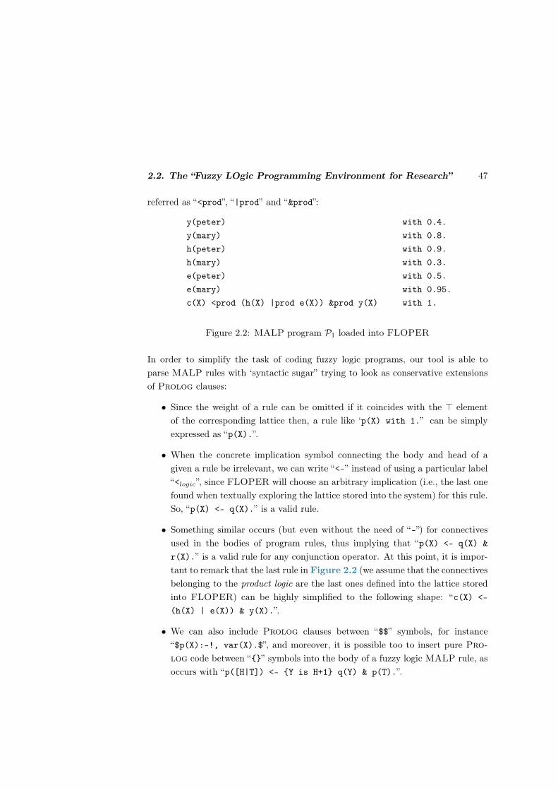
2.2. The “Fuzzy LOgic Programming Environment for Research” 47
referred as “<prod”, “|prod” and “&prod”:
y(peter) with 0.4.
y(mary) with 0.8.
h(peter) with 0.9.
h(mary) with 0.3.
e(peter) with 0.5.
e(mary) with 0.95.
c(X) <prod (h(X) |prod e(X)) &prod y(X) with 1.
Figure 2.2: MALP program P1 loaded into FLOPER
In order to simplify the task of coding fuzzy logic programs, our tool is able to
parse MALP rules with ‘syntactic sugar” trying to look as conservative extensions
of Prolog clauses:
• Since the weight of a rule can be omitted if it coincides with the ⊤ element
of the corresponding lattice then, a rule like ‘p(X) with 1.” can be simply
expressed as “p(X).”.
• When the concrete implication symbol connecting the body and head of a
given a rule be irrelevant, we can write “<-” instead of using a particular label
“<logic”, since FLOPER will choose an arbitrary implication (i.e., the last one
found when textually exploring the lattice stored into the system) for this rule.
So, “p(X) <- q(X).” is a valid rule.
• Something similar occurs (but even without the need of “-”) for connectives
used in the bodies of program rules, thus implying that “p(X) <- q(X) &
r(X).” is a valid rule for any conjunction operator. At this point, it is impor-
tant to remark that the last rule in Figure 2.2 (we assume that the connectives
belonging to the product logic are the last ones defined into the lattice stored
into FLOPER) can be highly simplified to the following shape: “c(X) <-
(h(X) | e(X)) & y(X).”.
• We can also include Prolog clauses between “$$” symbols, for instance
“$p(X):-!, var(X).$”, and moreover, it is possible too to insert pure Pro-
log code between “” symbols into the body of a fuzzy logic MALP rule, as
occurs with “p([H|T]) <- Y is H+1 q(Y) & p(T).”.

48 Chapter 2. Multi-adjoint Logic Programming and the FLOPER System
Figure 2.3: Running FLOPER into any standard Prolog platform
Once the application is loaded inside any standard Prolog interpreter (like SWI or
Sicstus -which is our case, by using v3.12.5-), it shows the menu shown in Figure
2.3. The parser has been implemented by using the classical DCG’s (Definite Clause
Grammars) resource of the Prolog language, since it is a convenient notation for
expressing grammar rules. Via the “parse” option, it is possible to load a “.fpl” file
for which FLOPER generates two different Prolog representations of the fuzzy
code, as we will describe in sub-sections 2.2.1 and 2.2.2. Such code will cohabit with
the set of clauses introduced by the user (together the Prolog-based definition of
the associated lattice that we will describe in sub-section 2.2.3) via the “load” option
for consulting pure Prolog files (“.pl”). The system is equipped too with choices

2.2. The “Fuzzy LOgic Programming Environment for Research” 49
Figure 2.4: The graphical interface of FLOPER
for saving and listing such rules as well as the “clean” option for removing all clauses
from the FLOPER database.
The remaining menus are useful for executing goals and displaying evaluation trees,
as well as for managing multi-adjoint lattices, as we are going to explain in what
follows helped by the graphical interface recently developed for FLOPERand shown
in Figure 2.4, which allows the comfortable use of “projects” in order to manage
files with the following different purposes:
• several “.fpl” files can contain the set of MALP rules implementing a single
MALP program,
• the set of clauses modeling its (unique) associated multi-adjoint lattice must
be included into a file with obvious extension “.pl”,
• additional Prolog code (for representing linguistic modifiers/variables, etc)
can be also attached in different “.pl” files and
• several “script” files could be useful for executing in one go more than one of

50 Chapter 2. Multi-adjoint Logic Programming and the FLOPER System
the set of commands we are going to explain in this section, as illustrated in
the following example:
ord: intro.
arg: c(X).
ord: ismode.
arg: s.
ord: tree.
ord: leaves.
ord: run.
2.2.1 Running Programs
In order to fully execute a goal, FLOPER employs the high-level representation
of the MALP program compiled via the “parse” option. The key point of this
code is to extend each atom of the program with an extra argument, called truth
variable, of the form TVi, which is intended to contain the truth degree obtained
after the subsequent evaluation of the atom. In the case of a fact, the extra argument
obviously contains its weight. For instance, “p(X) with 0.5” is simply translated
into the Prolog fact “p(X, 0.5)”.
Fuzzy connectives are represented as predicates defined in the lattice associated
to the program. For instance, the role of “&godel” is played by the Prolog predicate
“and_godel”. Since the fuzzy connective “&godel” is a binary operation, then its
associated predicate “and_godel” has arity three: two parameters plus the result,
returned in the third argument TV.
When compiling MALP rules, the last atom called in the body of the trans-
lated clause is the adjoint conjunction, which is intended to combine the truth de-
gree of the body and the weight of the rule, in order to propagate the final truth
degree to the head. For instance, given a MALP rule like “p(X) <prod q(X,Y)
&godel r(Y) with 0.8”, the resulting translated Prolog clause would look like
“p(X,_TV0) : −q(X, Y,_TV1), r(Y,_TV2), and_godel(_TV1,_TV2,_TV3), and_prod(0.8,_TV3,_TV0)”.
In order to execute a fuzzy program stored in a “.fpl” file , FLOPER needs firstly
to load and compile it by using the “parse” option. Internally, while FLOPER
analyzes the content of the file (following the DCG specification of the MALP
syntax) it also generates two different Prolog representations of the fuzzy code:
the high level representation coincides with a set of executable Prolog clauses as

2.2. The “Fuzzy LOgic Programming Environment for Research” 51
we have just described, while the low level representation allows FLOPER to draw
execution trees as we will see in the next subsection.
Here we have an example of using the “parse” option, where note that FLOPER
lists the content of any previously loaded “.pl” file (none in our case), the parsed
MALP program and the generated Prolog code.
>> parse.
File to parse: ‘P1.fpl’.
No loaded files.
ORIGINAL FUZZY-PROLOG CODE:
y(peter) with 0.4.
y(mary) with 0.8.
h(peter) with 0.9.
h(mary) with 0.3.
e(peter) with 0.5.
e(mary) with 0.95.
c(X) <prod (h(X) |prod e(X)) &prod y(X) with 1.
GENERATED PROLOG CODE:
y(peter,0.4).
y(mary,0.8).
h(peter,0.9).
h(mary,0.3).
e(peter,0.5).
e(mary,0.95).
c(X,TV0):-h(X,_TV1),e(X,_TV2),lat:or_prod(_TV1,_TV2,_TV3),
y(X,_TV4),lat:and_prod(_TV3,_TV4,_TV5),
lat:and_prod(1,_TV5,TV0).
While parsing, FLOPER creates a file tmp_fuzzy-prolog.pl to allocate the generated
Prolog code, in order to allow the possibility of saving it afterwards into a new file
by using the “save” option.
One important feature is that translated connectives (like “lat:and_prod/3”)
are prefixed by “lat:”, which means that the Prolog interpreter will search their

52 Chapter 2. Multi-adjoint Logic Programming and the FLOPER System
definitions in the “lat” module, a different name-space designed to avoid name
collisions. The resulting Prolog code can be executed in any Prolog engine, with
the only requirement that the associated lattice must be loaded in the corresponding
module. This can be easily achieved with the following two goals:
?- lat:consult(lattice.pl).
?- consult(program.fpl).
Moreover, goals are introduced in FLOPER by choosing the “intro” option and they
suffer a very similar translation process to program rules. So, it is easy to see that a
fuzzy goal like “y(X) &godel h(peter)”, is translated into the pure Prolog goal
“y(X, _TV1),h(peter, _TV2), and_godel(_TV1, _TV2, Truth_degree)” (note
that the last truth degree variable is not anonymous now) for which the Prolog
interpreter returns the two desired fuzzy computed answers after selecting the “run”
option (see Figure 2.4) :
[Truth_degree=0.4, X=peter]
[Truth_degree=0.8, X=mary]
2.2.2 Execution Trees
Apart from the compilation method to Prolog code commented before, we have
conceived a new low-level representation for the fuzzy code which is useful for build-
ing execution trees with any level of depth and offering too debugging (tracing)
capabilities. For instance, after parsing the last rule of our program, we obtain
the following expression (which is “asserted” into the database of the interpreter
as a Prolog fact, but it is never executed directly, in contrast with the previous
Prolog-based, high-level representation of the fuzzy code) whose components have
obvious meanings:
rule(7,
head(atom(pred(c,1),[var(’X’)])),
impl(prod),
body(and(prod,2,[or(prod,2,[atom(pred(h,1),[var(’X’)]),
atom(pred(e,1),[var(’X’)])]),
atom(pred(y,1),[var(’X’)])])),
td(1)).

2.2. The “Fuzzy LOgic Programming Environment for Research” 53
Figure 2.5: FLOPER drawing an execution tree
FLOPER is equipped with three options related with tracing tasks. Option “tree”
draws the execution tree (which collects a different derivation from the root to each
leaf) of a goal w.r.t. a program. Option “depth” fixes the maximum length allowed
for their branches (initially 3). And, finally, option “ismode” fixes the detail level of
the interpretive phase associated to each derivation in the tree.
So, let us consider again the MALP program of our running example. For goal
“y(X) &godel h(peter)”, FLOPER displays the tree showed in Figure 2.5. In
this screen-shot, we find two representations of the same tree: the middle-up window
shows the proper graphic which is easy to understand and manipulate (by moving
nodes, showing only skeletons of trees, etc.), while the marked text in the middle-
down window represents the same tree in plain text. In this last case, each line

54 Chapter 2. Multi-adjoint Logic Programming and the FLOPER System
Figure 2.6: Comparing different modes of performing the interpretive phase
contains a state (composed by the corresponding goal and substitution) preceded by
the number of the program rule used by the admissible step leading to it (root nodes
and nodes obtained via →AS3 are always labeled with the virtual, non existing rule
R0), and nodes belonging to the same branch appear in different lines appropriately
indented to help the readability of the tree (which only contain two different branches
in our case). Generated trees can be saved in “.jpg”, “.txt” and “xml” formats.
Moreover, FLOPER allows the user to choose the level of information given by
the interpretive phase in the execution tree through option “ismode”. We can choose
among the following three modes:

2.2. The “Fuzzy LOgic Programming Environment for Research” 55
• large: This mode omits the entire interpretive phase, offering only the final
leaf (if exists) of each branch.
• medium: Performs classical interpretive steps according Definition 2.1.5, in
order to evaluate each expression of the goal till finding the final solution.
• small: This mode applies our improved notion of small interpretive step pro-
vided in Definition 2.1.9, which is very useful for visualizing the more or less
complexity (distinguishing between connective calls and primitive operators
evaluation) of connectives exploited during the interpretive phase. Figure
2.6 shows that the shorter the step is, the larger tree is generated.
To finish this block, we are going to illustrate now with a very simple example
that the new options are crucial when the “run” choice fails: remember that this
last option is based on the generation of pure logic SLD-derivations which might
fall in loop or directly fail when finding non defined atoms, in contrast with the
traces (based on finite, non- failed, admissible/interpretive derivations) that the
“tree” option displays. So, consider the following MALP program:
p(a) with 0.8.
p(X) <prod p(s(s(s(X)))) with 0.9.
p(b) with 0.6.
where the first and last rules indicate that a goal like “p(X)” admits two solutions, but
the second rule would be responsible of introducing an infinite branch between the
leaves associated to both fuzzy computed answers in the corresponding execution
tree. Moreover, if we plan to run a more complex goal like “q(X) @aver p(X)”
(where, obviously, the used connective refers to the average aggregator), we find a
second problem related now with an undefined atom. In contrast with Prolog,
in our fuzzy setting the evaluation of “q(X)” doesn’t fail, since FLOPER proceeds
with an →AS3 step according Definition 2.1.2, and hence, it is possible to find the
two desired fuzzy computed answers for that goal, as shown in the execution tree of
Figure 2.7. By choosing option “leaves”, the system displays the content of the two
fully evaluated leaves “<0.4,X/a>” and “<0.3,X/b>”, as desired.
As we have seen, the generation of traces based on execution trees, contribute to
increase the power of FLOPER by providing debugging capabilities which allow us
to discover solutions for queries even when the pure Prolog compilation-execution
process becomes insufficient.

56 Chapter 2. Multi-adjoint Logic Programming and the FLOPER System
Figure 2.7: Tree with an infinite branch and a →AS3 step
2.2.3 Managing Lattices
We have conceived a very easy way to model lattices of truth degrees for being
included into the FLOPER tool. All relevant components of each lattice can be
encapsulated inside a Prolog file which must necessarily contain the definitions
of a minimal set of predicates defining the set of valid elements (including special
mentions to the “top” and “bottom” ones), the full or partial ordering established
among them, as well as the repertoire of fuzzy connectives which can be used for
their subsequent manipulation. In order to simplify our explanation, assume that file
“bool.pl” refers to the simplest notion of (a binary) adjoint lattice, thus implementing
the following set of predicates:
• member/1 which is satisfied when being called with a parameter representing a
valid truth degree. In the case of finite lattices, it is also recommended to imple-
ment members/1 which returns in one go a list containing the whole set of truth
degrees. For instance, in the Boolean case, both predicates can be simply mod-
eled by the Prolog facts: member(0)., member(1). and members([0,1]).
• bot/1 and top/1 obviously answer with the top and bottom element of the
lattice, respectively. Both are implemented into “bool.pl” as bot(0). and

2.2. The “Fuzzy LOgic Programming Environment for Research” 57
top(1).
• leq/2 models the ordering relation among all the possible pairs of truth de-
grees, and obviously it is only satisfied when it is invoked with two elements
verifying that the first parameter is equal or smaller than the second one. So,
in our example it suffices with including into “bool.pl” the facts: leq(0,X).
and leq(X,1).
• Finally, given some fuzzy connectives of the form &label1 (conjunction), |label2(disjunction) or @label3 (aggregation) with arities n1, n2 and n3 respectively, we
must provide clauses defining the connective predicates “and_label1/(n1+1)”,
“or_label2/(n2+1)” and “agr_label3/(n3+1)”, where the extra argument of each
predicate is intended to contain the result achieved after the evaluation of the
proper connective. For instance, in the Boolean case, the following two facts
model in a very easy way the behaviour of the classical conjunction operation:
and_bool(0,_,0). and_bool(1,X,X).
The reader can easily check that the use of lattice “bool.pl” when working with
MALP programs whose rules have the form “A ←bool &bool(B1, . . . , Bn) with 1”,
being A and Bi typical atoms1, successfully mimics the behaviour of classical Pro-
log programs where clauses accomplish with the shape “A : − B1, . . . , Bn”.
As a novelty in the fuzzy setting, when evaluating goals according to the procedural
semantics described in Section 2.1.1, each output will contain the corresponding sub-
stitution (i.e., the crisp notion of computed answer obtained by means of classical
SLD-resolution in Prolog) together with the maximum truth degree 1.
On the other hand and following the Prolog style regulated by the previous
guidelines, in file “num.pl” we have included the clauses shown in Figure 2.8. Here,
we have modeled the more flexible lattice (that we will mainly use in our examples,
beyond the boolean case) which enables the possibility of working with truth degrees
in the infinite space (note that this condition disables the implementation of the
consulting predicate “members/1”) of real numbers between 0 and 1, allowing too
the possibility of using conjunction and disjunction operators recasted from the three
typical fuzzy logics described before (i.e., the Łukasiewicz, Gödel and product logics),
as well as a useful description for the hybrid aggregator average.
1Here we also assume that several versions of the classical conjunction operation have been
implemented with different arities.

58 Chapter 2. Multi-adjoint Logic Programming and the FLOPER System
member(X) :- number(X),0=<X,X=<1. %% no members/1 (infinite lattice)
bot(0). top(1). leq(X,Y) :- X=<Y.
and_luka(X,Y,Z) :- pri_add(X,Y,U1),pri_sub(U1,1,U2),pri_max(0,U2,Z).
and_godel(X,Y,Z):- pri_min(X,Y,Z).
and_prod(X,Y,Z) :- pri_prod(X,Y,Z).
or_luka(X,Y,Z) :- pri_add(X,Y,U1),pri_min(U1,1,Z).
or_godel(X,Y,Z) :- pri_max(X,Y,Z).
or_prod(X,Y,Z) :- pri_prod(X,Y,U1),pri_add(X,Y,U2),pri_sub(U2,U1,Z).
agr_aver(X,Y,Z) :- pri_add(X,Y,U),pri_div(U,2,Z).
pri_add(X,Y,Z) :- Z is X+Y. pri_min(X,Y,Z) :- (X=<Y,Z=X;X>Y,Z=Y).
pri_sub(X,Y,Z) :- Z is X-Y. pri_max(X,Y,Z) :- (X=<Y,Z=Y;X>Y,Z=X).
pri_prod(X,Y,Z) :- Z is X * Y. pri_div(X,Y,Z) :- Z is X/Y.
Figure 2.8: Multi-adjoint lattice modeling truth degrees in the real interval [0,1]
(“num.pl”)
Note also that we have included definitions for auxiliary predicates, whose names
always begin with prefix “pri_”. All of them are intended to describe primitive/arith-
metic operators (in our case +, −, ∗, /, min and max) in a Prolog style, for being
appropriately called from the bodies of clauses defining predicates with higher levels
of expressiveness (this is the case for instance, of the three kinds of fuzzy connectives
we are considering: conjunctions, disjunctions and agreggations).
Since till now we have considered two classical, fully ordered lattices (with a
finite and infinite number of elements, collected in files “bool.pl” and “num.pl”, re-
spectively), we wish now to introduce a different case coping with a very simple
lattice where not always any pair of truth degrees are comparable. So, consider the
partially ordered multi-adjoint lattice in Figure 2.9 for which the conjunction and
implication connectives based on the Gödel logic described in Section 2.1.1 conform
an adjoint pair but with the particularity now that, in the general case, the Gödel ’s
conjunction must be expressed as &G(x, y) , inf(x, y), where it is important to
note that we must replace the use of “min” by “inf ” in the connective definition.
To this end, observe in the Prolog code accompanying Figure 2.9 that we have
introduced five clauses defining the new primitive operator “pri_inf/3” which is
intended to return the infimum of two elements. Related with this fact, we must
point out the following aspects:

2.2. The “Fuzzy LOgic Programming Environment for Research” 59
⊤
α β
⊥
member(bottom). member(alpha).
member(beta). member(top).
members([bottom,alpha,beta,top]).
leq(bottom,X). leq(alpha,alpha).
leq(beta,beta). leq(beta,top).
leq(alpha,top). leq(X,top).
and_godel(X,Y,Z) :- pri_inf(X,Y,Z).
pri_inf(bottom,X,bottom):-!.
pri_inf(alpha,X,alpha):-leq(alpha,X),!.
pri_inf(beta,X,beta):-leq(beta,X),!.
pri_inf(top,X,X):-!.
pri_inf(X,Y,bottom).
Figure 2.9: Partially ordered lattice with four elements
• Note that since truth degrees α and β -or their corresponding representations
as Prolog terms “alpha” and “beta” used for instance in the definition(s)
of “members(s)/1”- are not comparable, any call to “leq(alpha,beta)” or
“leq(beta,alpha)” will always fail.
• However, goals “pri_inf(alpha,beta,X)” and “pri_inf(beta,alpha,X)”, in-
stead of failing, successfully produces the desired result “X=bottom”.
• Note anyway that the implementation of the “pri_inf/1” predicate is manda-
tory for coding the general definition of “and_godel/3”.
As a final example, we can also define the so called Borel algebra based on the unionof intervals (where for instance B([0, 1]) is the union of intervals between 0 and 1[VGM02, MCS11]) as a Prolog program for being used into FLOPER as follows:
member([i(X,Y)]) :- number(X),number(Y),X=<Y.
member([i(X,Y),i(Z,T)|U]) :- number(X),number(Y),number(Z),
X=<Y, Y < Z,member([i(Z,T)|U]).
bot([i(0,0)]). top([i(1,1)]).
leq([X1,X2|X],Y) :- existsGreater(X1,Y),leq([X2|X],Y).
leq([X1],Y) :- existsGreater(X1,Y).
existsGreater(i(Xb,Xt),[i(Yb,Yt)|Y]) :- Yb=<Xb, Xt=<Yt,!.
existsGreater(X,[_|Y]) :- existsGreater(X,Y).
• A member of this algebra is a list of pairs representing disjoined intervals.

60 Chapter 2. Multi-adjoint Logic Programming and the FLOPER System
• The top element is the point 1 (interval from 1 to 1), and the bottom one is
the point 0 (interval from 0 to 0).
• A union of intervals, U , is less or equal than other union of intervals U ′ if for
each I ∈ U , there exists another interval I ′ ∈ U ′, such that I ⊆ I ′.
2.2.4 Linguistic modifiers and linguistic variables
Another interesting feature of FLOPER is its ability for managing linguistic modi-
fiers and linguistic variables in a very easy way. A linguistic modifier can be seen as
an aggregator such that, when applied to a fuzzy expression, it alters its final truth
degree. Some examples of well known modifiers are “very” and “roughly”, where the
first one tends to return a lower truth degree, and the second one, a higher truth de-
gree. Since the concept of modifier is dependent of a concrete lattice, its definition
should appear inside the Prolog file containing the proper multi-adjoint lattice
loaded into FLOPERFor instance, in the typical lattice 〈[0, 1],≤〉 used in previous
examples, we could define some modifiers by means of the following usual formulae:
modifier formula implementation
extremely extremely(x) = x4 agr_extremely(X,TV0) : −TV0 is X ∗X ∗X ∗X.very very(x) = x2 agr_very(X,TV0) : −TV0 is X ∗X.moreorless moreless(x) = x1/2 agr_moreless(X,TV0) : −TV0 is sqrt(X).
roughly roughly(x) = x1/4 agr_roughly(X,TV0) : −TV0 is sqrt(sqrt(X)).
Figure 2.10: Linguistic modifiers
With these modifiers, now we could update the program of Figure 2.1 to increase
the difficulty for obtaining a credit in crisis times. The only rule to be modified is

2.2. The “Fuzzy LOgic Programming Environment for Research” 61
the seventh one, whose new shape could look like:
R∗7 : c(X) ←p @very((h(X) |P e(X)) &P y(X)) with 1
Linguistic modifiers increase the expresiveness of the fuzzy language and as said
before, they have to be defined as part of the lattice associated to the MALP
program in the current project.
On the other hand, linguistic variables allow us to represent linguistic symbols
defined by means of fuzzy sets. A linguistic variable is characterized by a tuple
〈x, T, U,G,M〉, where x is the name of the variable, T the set of linguistic symbols
or terms of x, U the universe where x is defined, G represents a syntactic rule to
generate linguistic terms, and M is a semantic rule for assigning to each linguistic
symbol t its fuzzy set M(t). For instance, we can represent the linguistic variable
distance, with values near, far_away defined over the universe [0,+∞) in kilo-
meters, as shown in Figure 2.11. We can implement this variable into a Prolog
file defining a fuzzy predicate for each symbol. The arguments are an input vari-
able (D) giving the crisp distance, and an output variable (TV) returning the degree
of membership of the input variable to the fuzzy set. Then, it is possible to load
this Prolog program into the current project of FLOPER, in order to use such
definitions in the corresponding MALP program.
Figure 2.11: Linguistic variable “distance” with terms “near” and “far away”
near(D,1) :- D=<100.
near(D,TV):- 100<X, X=<500, TV is (500-X)/400.
near(D,0) :- 500<D.
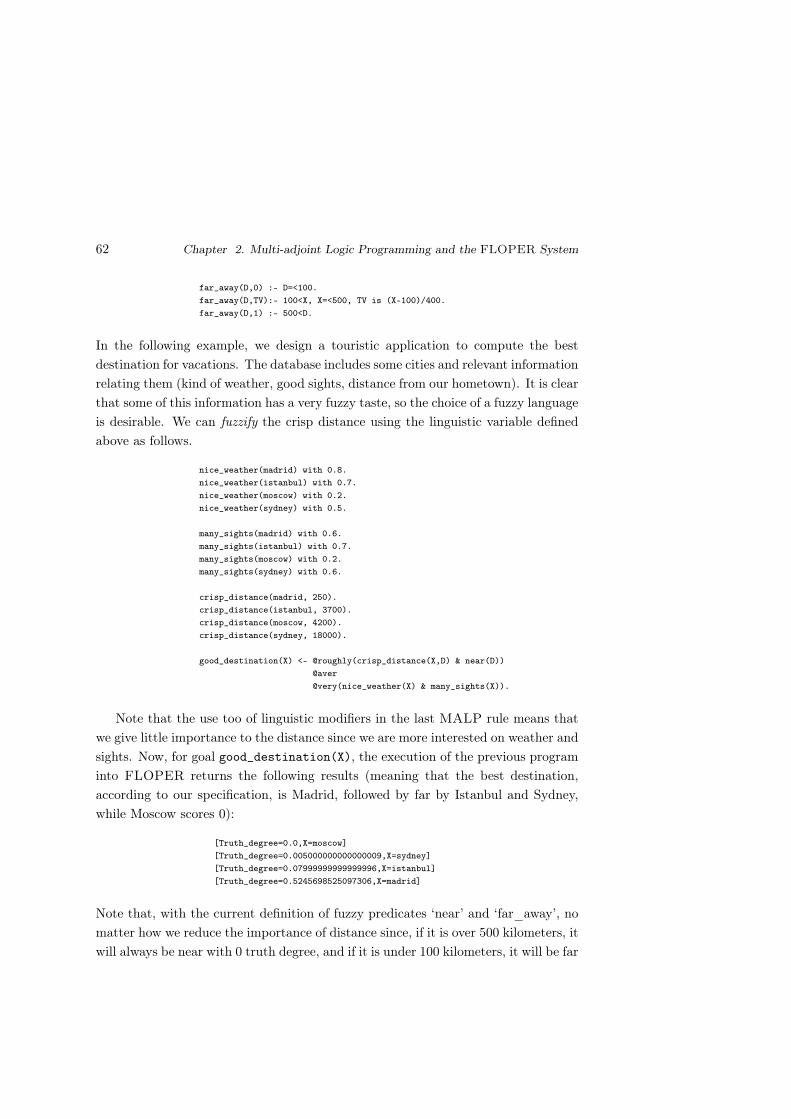
62 Chapter 2. Multi-adjoint Logic Programming and the FLOPER System
far_away(D,0) :- D=<100.
far_away(D,TV):- 100<X, X=<500, TV is (X-100)/400.
far_away(D,1) :- 500<D.
In the following example, we design a touristic application to compute the best
destination for vacations. The database includes some cities and relevant information
relating them (kind of weather, good sights, distance from our hometown). It is clear
that some of this information has a very fuzzy taste, so the choice of a fuzzy language
is desirable. We can fuzzify the crisp distance using the linguistic variable defined
above as follows.
nice_weather(madrid) with 0.8.
nice_weather(istanbul) with 0.7.
nice_weather(moscow) with 0.2.
nice_weather(sydney) with 0.5.
many_sights(madrid) with 0.6.
many_sights(istanbul) with 0.7.
many_sights(moscow) with 0.2.
many_sights(sydney) with 0.6.
crisp_distance(madrid, 250).
crisp_distance(istanbul, 3700).
crisp_distance(moscow, 4200).
crisp_distance(sydney, 18000).
good_destination(X) <- @roughly(crisp_distance(X,D) & near(D))
@aver
@very(nice_weather(X) & many_sights(X)).
Note that the use too of linguistic modifiers in the last MALP rule means that
we give little importance to the distance since we are more interested on weather and
sights. Now, for goal good_destination(X), the execution of the previous program
into FLOPER returns the following results (meaning that the best destination,
according to our specification, is Madrid, followed by far by Istanbul and Sydney,
while Moscow scores 0):
[Truth_degree=0.0,X=moscow]
[Truth_degree=0.005000000000000009,X=sydney]
[Truth_degree=0.07999999999999996,X=istanbul]
[Truth_degree=0.5245698525097306,X=madrid]
Note that, with the current definition of fuzzy predicates ‘near’ and ‘far_away’, no
matter how we reduce the importance of distance since, if it is over 500 kilometers, it
will always be near with 0 truth degree, and if it is under 100 kilometers, it will be far

2.3. Extending Lattices and Declarative Traces 63
with 0 truth degree. If our perception of distance changes, these notions will become
useless. To fix that, we can define them with non-linear rules like the following ones,
which show that FLOPER is flexible enough to deal with fuzzy predicates defined
(in Prolog) by means of non-linear arithmetic expressions:
near(D,TV) :- TV is 250/(D+250).
far(D,TV) :- TV is 1 - 250/(D+250).
Figure 2.12: Linguistic variable “distance” with flexible versions of “near” and “far
away”
2.3 Extending Lattices and Declarative Traces
This section presents different methods to gain expressiveness when designing a
MALP program by manipulating its associated lattice. The main technique con-
sists on agglutinating several lattices in order to obtain the Cartesian product of
them, which is also a multi-adjoint lattice [MMPV12a]. Once this is done, a new
functionality emerges for obtaining declarative traces (when evaluating goals) at a
very low cost.
Teorema 2.3.1. If L1, . . . , Ln are a finite number of multi-adjoint lattices, then its
Cartesian product L = L1 × · · · × Ln is also a multi-adjoint lattice.
In order to simplify our explanation, but without lost of generality, we only
consider two multi-adjoint lattices (L1,≤1,&1,←1) and (L2,≤2,&2,←2), each one

64 Chapter 2. Multi-adjoint Logic Programming and the FLOPER System
equipped with just a single adjoint pair. Then, L = L1×L2 has lattice structure with
an ordering relation induced in the product from (L1,≤1) and (L2,≤2) as follows:
(x1, y1) ≤ (x2, y2)⇔ x1 ≤1 x2, y1 ≤2 y2
Moreover, being ⊤1 = sup(L1), ⊥1 = inf(L1), ⊤2 = sup(L2) and ⊥2 = inf(L2),
we have that (⊤1,⊤2) = sup(L) and (⊥1,⊥2) = inf(L) which implies that the
Cartesian product L is a bounded lattice if both L1 and L2 are also bounded lattices.
Analogously, L1×L2 is a complete lattice if L1 and L2 verify too the same property.
Finally, from the adjoint pairs (&1,←1) and (&2,←2) in L1 and L2, respectively, it
is possible to define the following connectives in L:
(x1, y1)&(x2, y2) , (x1&1x2, y1&2y2)
(x1, y1)← (x2, y2) , (x1 ←1 x2, y1 ←2 y2)
for which it is easy to justify that they conform an adjoint pair in L1 × L2 (thus
satisfying, in particular, the adjoint property). In a similar way, it is also possible to
define new connectives (conjunctions, disjunctions and aggregators) in the Cartesian
product L1 × L2 from the corresponding pairs of operators defined in L1 and L2.
FLOPER is able to deal with Cartesian products of multi-adjoint lattices by
acting on the “member/1” predicate, which accept as argument any object which
belong to a lattice. Some examples of simple “member/1” definitions are:
• member(X) :- number(X), X=<1, X>=0: [0,1] interval
• member([X|L]): lists
• member(info(X,Y)): pairs
The very intuitive way to obtain Cartesian product of lattices is to use Prolog
functions with arity 2 (indeed, the cartesian product of n lattices can be represented
using functions with arity n). In order to implement a cartesian product of lattices
in a Prolog file, we define “member/1” predicate whose parameter is a term headed
with a function symbol, for instance: member(f(X,Y)) :- check1(X), check2(Y).
Of course, predicates “leq/2”, “top/1”, “bot/1” and connectives have to be defined
following the same criterium in order to implement the concrete Cartesian product
of lattices.
Before showing an example of Cartesian product modeled in FLOPER, let us
consider again the so called domain of weight values W used in the QLP (Qualified

2.3. Extending Lattices and Declarative Traces 65
Logic Programming framework of [RD08, CRR10, RR08a], whose elements are in-
tended to represent proof costs, measured as the weighted depth of proof trees. As
explained in Section 2.1, W can be seen as lattice (N ∪ ∞,≥), where ≥ is the
reverse of the usual numerical ordering (with ∞ ≥ d for any d ∈ N) and thus, the
bottom elements is ∞ and the top element is 0 (and not vice versa). Note that in
this lattice the arithmetic operation “+” plays the role of a conjunction (it is easy
to prove that in this setting such definition of & verifies the properties required
by t-norms [NW06]). Moreover, we can obtain the residual implication of the “+”
t-norm, defined as y ← z , supt ∈ W : t + z ≤ y, which in this particular case
acquires the following shape:
y ← z ,
y − z, if z ≥ y
0, if y > z
So, the reader can easily check that (+,←) conforms an adjoint pair in (N∪∞,≥),thus accomplishing with Definition 2.1.1 in Section 2.1, which implies that W is
in fact a multi-adjoint lattice. A valid implementation of W lattice presents the
following definitions:
member(X) :- number(X). member(infty).
leq(infty,X). leq(X,Y):-X>=Y.
top(0). bot(infty).
and_plus(X,infty,infty). and_plus(infty,X,infty). and_plus(X,Y,Z):-Z is X+Y.
In order to associate the lattice W to our program P1, we have to change the
weights of each rule by valid truth degrees belonging to the new lattice. For instance,
rule “y(peter) with 0.4” would be rewritten as “y(peter) with 1” (the underlying idea
is that “the use of each program rule in a derivation implies the application of one
admissible step”), resulting in a new program, PW . By using the “lat” option of
FLOPER, we can built a project which associates lattice W to program PW and
now, for goal “c(X)”, we can generate an admissible derivation similar to the one seen
in Figure 2.1, but ending now with 〈&P(info(1,&P(|P(1, 1), 1)), X/peter〉. Since:
&P(1,&P(|P(1, 1), 1)) = +(1,+(+(1, 1), 1))) = 4, the final fuzzy computed answer or
f.c.a. 〈4; X/peter〉 indicates that goal “c(X)” holds when X is peter, as proved
after applying 4 admissible steps.
On the other hand, since we have said that V is the multi-adjoint lattice ([0, 1],≤)based on real numbers in the unit interval used along this thesis (which is equipped
with three adjoint pairs modeling implication and conjunction symbols collected

66 Chapter 2. Multi-adjoint Logic Programming and the FLOPER System
from the Łukasiewicz logic, Gödel intuitionistic logic and product logic) then, in the
Cartesian product V×W we will find the top and bottom elements (1, 0) and (0,∞),
respectively, as well as the following definitions of conjunction operations (among
other connectives) whose names are mirroring to extensions of the product logic and
Łukasiewicz logic:
(v1, w1) &P+ (v2, w2) , (v1 ∗ v2, w1 + w2)
(v1, w1) &L+ (u2, w2) , (max(0, v1 + v2 − 1), w1 + w2)
Moreover, we can also conceive a more powerful lattice expressed as the Cartesian
product of V (see Figure 2.8) andW. Now, each element includes two components,
coping with truth degrees and cost measures. In order to be loaded into FLOPER,
we must define in Prolog the new lattice, whose elements could be expressed as
data terms of the form “info(Fuzzy_Truth_Degree, Cost_Number_Steps)”. Some
of the required predicates are:
member(info(X,W)):-number(X), 0=<X,X=<1,(W=infty,!; number(W),1=<W).
leq(info(X1,W1),info(X2,W2)):-X1 =< X2, (W1=infty,!; number(W2), W2 =< W1).
bot(info(0,infty)). top(info(1,1)).
and_prod(info(X,W1),info(Y,W2),info(Z,W3)) :- pri_prod(X,Y,Z),pri_add(W1,W2,W3).
pri_add(infty,_,infty). pri_add(_,infty,infty).
pri_add(X,Y,Z) :- number(X), number(Y), Z is X+Y.
Finally, if the weights assigned to the rules of our example are “info(0.4,1)” forR1,
“info(0.8,1)” for R2, “info(0.9,1)” for R3 and so on, then we would obtain the
desired f.c.a. 〈info(0.38, 4); X/peter〉 for goal “c(X)”, with the obvious meaning
that we need 4 admissible steps to prove that the query is true at a 38% degree when
X is “peter”.
One step beyond, we will also see that if instead of the number of computational
steps, we are interested in knowing more detailed data about the set of program rules
and connective definitions evaluated for obtaining each solution then, instead of Wit will be mandatory to use a new lattice S based on strings or labels (i.e., sequences
of characters) for generating the Cartesian product V × S. In [MMPV12b] we show
not only that S is a complete multi-adjoint lattice, but also that the concatenation
of strings, usually called “append” in many programming languages, plays the role
of a conjunction connective in such lattice.

2.3. Extending Lattices and Declarative Traces 67
In order to be loaded into FLOPER, we need to define again the new lattice as a
Prolog program, whose elements will be terms of the form
“info(Fuzzy_Truth_Degree, Label)” as shown in Figure 2.13 (we only list some
representative clauses).
member(info(X,Y)):-number(X),0=<X,X=<1,atom(Y). top(info(1,’’)).
and_prod(info(X1,X2),info(Y1,Y2),info(Z1,Z2)) :-
pri_prod(X1,Y1,Z1,DatPROD),pri_app(X2,Y2,Dat1),
pri_app(Dat1,’&PROD.’,Dat2),pri_app(Dat2,DatPROD,Z2).
pri_prod(X,Y,Z,’#PROD.’):-Z is X * Y.
pri_app(X,Y,Z) :-name(X,L1),name(Y,L2),append(L1,L2,L3),name(Z,L3).
append([],X,X). append([X|Xs],Y,[X|Zs]):-append(Xs,Y,Zs).
.....
Figure 2.13: Multi-adjoint lattice modeling truth degrees with labels
Here, we see that when implementing for instance the conjunction operator of the
Product logic, in the second component of our extended notion of “truth degree”, we
have appended the labels of its arguments with label ’&PROD.’ (see clauses defining
and_prod, pri_app and append). Of course, in the fuzzy program to be run, we
must also take into account the use of labels associated to the program rules, as
occurs with the following example:
p(X) <prod &godel(q(X),@aver2(r(X),s(X))) with info(0.9,’RULE1.’).
q(a) with info(0.8,’RULE2.’).
r(X) with info(0.7,’RULE3.’).
s(X) with info(0.5,’RULE4.’).
where we have used in the first rule aggregator “@aver2” (intended to compute the
average between the results achieved by applying two different disjunction operations
on the parameters) defined in Prolog as:
agr_aver2(X,Y,info(Za,Zb)) :- or_godel(X,Y,Z1),or_luka(X,Y,Z2),
agr_aver(Z1,Z2,info(Za,Zc)),
pri_app(Zc,’@AVER2.’,Zb).
Now, the reader can easily test that, after executing goal “p(X)”, we obtain
the following fuzzy computed answer which includes the desired declarative trace
containing the sequence of program-rules and connective-calls (mirroring →AS and
→SIS1 steps, according definitions 2.1.2 and 2.1.9, respectively) evaluated till finding
the final solution:

68 Chapter 2. Multi-adjoint Logic Programming and the FLOPER System
>> run.
[Truth_degree=info(0.72, RULE1.RULE2.RULE3.RULE4.
@AVER2.|GODEL.|LUKA.
@AVER.&GODEL.&PROD.), X=a]
With a very little extra effort, we can extend the previous lattice to have into
account also the exploited primitive operators during the interpretive phase, thus
simulating →SIS2 steps (see again Definition 2.1.9). We simply need to include a
label in the Prolog definition of each primitive operator in order to identify it (for
instance, ”#PROD” refers to the product primitive operator).
and_prod(info(X1,X2),info(Y1,Y2),info(Z1,Z2)) :-
pri_prod(X1,Y1,Z1,DatPROD),pri_app(X2,Y2,Dat1),
pri_app(Dat1,’&PROD.’,Dat2),pri_app(Dat2,DatPROD,Z2).
pri_prod(X,Y,Z,’#PROD.’) :- Z is X * Y.
Figure 2.14: Obtaining declarative traces on fuzzy computed answers
As shown in Figure 2.14, the result of executing again goal “p(X)” is:
>> run.
[Truth_degree=info(0.72, RULE1.RULE2.RULE3.RULE4.
@AVER2.|GODEL.#MAX.|LUKA.
#ADD.#MIN.@AVER.#ADD.#DIV.
&GODEL.#MIN.&PROD.#PROD.), X=a]

2.3. Extending Lattices and Declarative Traces 69
In this fuzzy computed answer we obtain both the truth value (0.72) and sub-
stitution (X = a) associated to our goal, but also the sequence of program rules
exploited when applying admissible steps as well as the proper fuzzy connectives
evaluated during the interpretive phase, also detailing the set of primitive operators
(of the form #label) they call.

70 Chapter 2. Multi-adjoint Logic Programming and the FLOPER System

Chapter 3
The FuzzyXPath interpreter
In this chapter we present a fuzzy variant of the XPath query language for the
flexible information retrieval on XML documents. Our main purpose is to provide a
repertoire of operators that offer the possibility of managing satisfaction degrees by
adding structural constraints and fuzzy operators inside conditions (which must be
considered from now on as fuzzy conditions instead of boolean conditions), in order
to produce a ranked sorted list of answers according to user’s preferences when
composing queries. By using the FLOPER system designed in our research group,
our proposal has been implemented with a fuzzy logic language to take profit of the
clear synergies between both target and source fuzzy languages.
Our approach firstly proposes two structural constraints called DOWN and DEEP
for which a certain degree of relevance can be associated. So, whereas DOWN pro-
vides a ranked set of answers depending on the path they are found from “top to
down” in the XML document, DEEP provides a ranked set of answers depending on
the path they are found from “left to right” in the XML document. Both structural
constraints can be used together, assigning degree of importance with respect to the
distance to the root XML element.
Secondly, we have enriched the arsenal of operators of XPath with fuzzy variants
of and and or. Particularly, we have considered three versions of and: and+, and,
and- (and the same for or : or+, or, or-) which make more flexible the composition
of fuzzy conditions. Three versions for each operator that come for free from our
adaptation of fuzzy logic to the XPath paradigm. One of the most known elements
of fuzzy logic is the introduction of fuzzy versions of classical boolean operators.
71

72 Chapter 3. The FuzzyXPath interpreter
Product, Łukasiewicz and Gödel fuzzy logics are considered as the most prominent
logics and give a suitable semantics to fuzzy operators. Our contribution is now to
give sense to fuzzy operators into the XPath paradigm, and particularly in user’s
preferences. We claim that in our work the fuzzy versions provide a mechanism
to force (and debilitate) conditions in the sense that stronger (and weaker) user
preferences can be modeled with the use of stronger (and weaker) fuzzy conditions.
The combination of fuzzy operators in queries permits to specify a ranked set of
fuzzy conditions according to user’s requirements.
Finally, we have equipped our XPath based query language with a mechanism for
thresholding user’s preferences, in such a way that user can request that requirements
are satisfied over a certain percentage.
3.1 A Flexible XPath Language
Our proposal of flexible XPath is defined by the following grammar:
xpath := [‘[’deep-down‘]’ ]path
path := literal | text() | node | @att | node/path | node//path
node := QName | QName[cond]
cond := xpath op xpath | xpath num-op number
deep := DEEP=number
down := DOWN=number
deep-down := deep | down | deep ‘;’ down
num-op := > | = | < | <>
fuzzy-op := and | and+ | and- | or | or+ | or- |
avg | avgnumber,number
op := num-op | fuzzy-op
Basically, our proposal extends XPath as follows:
• A given XPath expression can be adorned with «[DEEP = r1; DOWN = r2]»
which means that the deepness of elements is penalized by r1 and that the order
of elements is penalized by r2, and such penalization is proportional to the
distance (i.e., the length of the branch and the weight of the tree, respectively).
In particular, «[DEEP = 1; DOWN = r2]» can be used for penalizing only
w.r.t. document order. DEEP works for //, that is, the deepness in the

3.1. A Flexible XPath Language 73
&P(x, y) = x ∗ y |P(x, y) = x+ y − x ∗ y Product: and/or
&G(x, y) = min(x, y) |G(x, y) = max(x, y) Gödel: and+/or-
&L(x, y) = max(x+ y − 1, 0) |L(x, y) = min(x+ y, 1) Łuka: and-/or+
Figure 3.1: Fuzzy Logical Operators
XML tree is only computed when descendant nodes are explored, while DOWN
works for both / and //. Let us remark that DEEP and DOWN can be used
several times on the main path expression and/or any other sub-path included
in conditions.
• We consider three versions for each one of the conjunction and disjunction
operators (also called connectives or aggregators) which are based in the so-
called Product, Gödel and Łukasiewicz fuzzy logics. The Gödel and Łukasiewicz
logic based fuzzy symbols 1 are represented in our application by and+, and-,
or- and or+, in contrast with product logic operators and and or (see Figure
3.1). Adjectives like pessimistic, realistic and optimistic are sometimes applied
to the Łukasiewicz, Product and Gödel fuzzy logics since operators satisfy that,
for any pair of real numbers x and y in [0, 1] (as used in MALPMALP):
0 ≤ &L(x , y) ≤ &P(x , y) ≤ &G(x , y) ≤ 1
and the contrary for the disjunction operations (as used in MALP):
0 ≤ |G(x , y) ≤ |P(x , y) ≤ |L(x , y) ≤ 1
So, note that it is more difficult to satisfy a condition based on a pessimistic
conjuntor/disjunctor (i.e, and-/or- inspired by the Łukasiewicz and Gödel log-
ics, respectively) than with Product logic based operators (i.e, and/or), while
the optimistic versions of such connectives (i.e., and+/or+) are less restrictive,
obtaining a greater set of answers. This is a consequence of the following chain
of inequalities (as used in MALP):
0 ≤ &L(x , y) ≤ &P(x , y) ≤ &G(x , y) ≤ |G(x , y) ≤ |P(x , y) ≤ |L(x , y) ≤ 1
or equivalently, by using the notation of our application:
0 ≤ and−(x , y) ≤ and(x , y) ≤ and+(x , y) ≤ or−(x , y) ≤ or(x , y) ≤ or+(x , y) ≤ 1
1The fuzzy logic community frequently uses the terms t-norm and t-conorm for expressing
generalized versions of conjunctions and disjunctions.

74 Chapter 3. The FuzzyXPath interpreter
Therefore users should refine queries by choosing operators in the previous
sequence from left to right (or from right to left), till finding solutions satisfying
in a stronger (or weaker) way the requirements.
• Furthermore, the avg operator is defined too in a weighted way. Assuming two
given RSV’s r1 and r2, avg is defined as (r1 + r2)/2, and avg(p1, p2) is defined
as (p1 ∗ r1 + p2 ∗ r2)/p1 + p2.
• Finally, we have considered a special case of constraint, a thresholding con-
straint of the form xpath op r, where r ∈ [0, 1] and op ∈ <,>,=, in which
the user can specify the threshold that the RSV of a given fuzzy condition has
to raise.
In general, an extended XPath expression defines, w.r.t. an XML document, a
sequence of subtrees of the XML document where each subtree has an associated
RSV. XPath conditions, which are defined as fuzzy operators applied to XPath
expressions, compute a new RSV from the RSVs of the involved XPath expressions,
which at the same time, provides an RSV to the node.
3.2 Examples with DEEP and DOWN
In order to illustrate the language, let us see some examples of flexible queries in
XPath. We will take as input document the one shown in Figure 3.2. The example
shows a sequence of hotels where each one is described by name and price, proximity
to streets (close_to) and provided services (pool and metro -together with distance-).
In the example, we assume that document order has the following semantics. The
tag close_to specifies the proximity to a given street. However, the order of close_to
tags is relevant, and the top streets are closer than the streets at the bottom. In
other words, the case:
hotel_H
close_to street_A
close_to street_B
implies that hotel H is near to both streets A and B, but closer to A than to B.
The nesting of close_to has also a relevant meaning. While a given street A can be
close to the hotel H, the streets close to A are not necessarily close to the hotel H.
In other words, in the case:
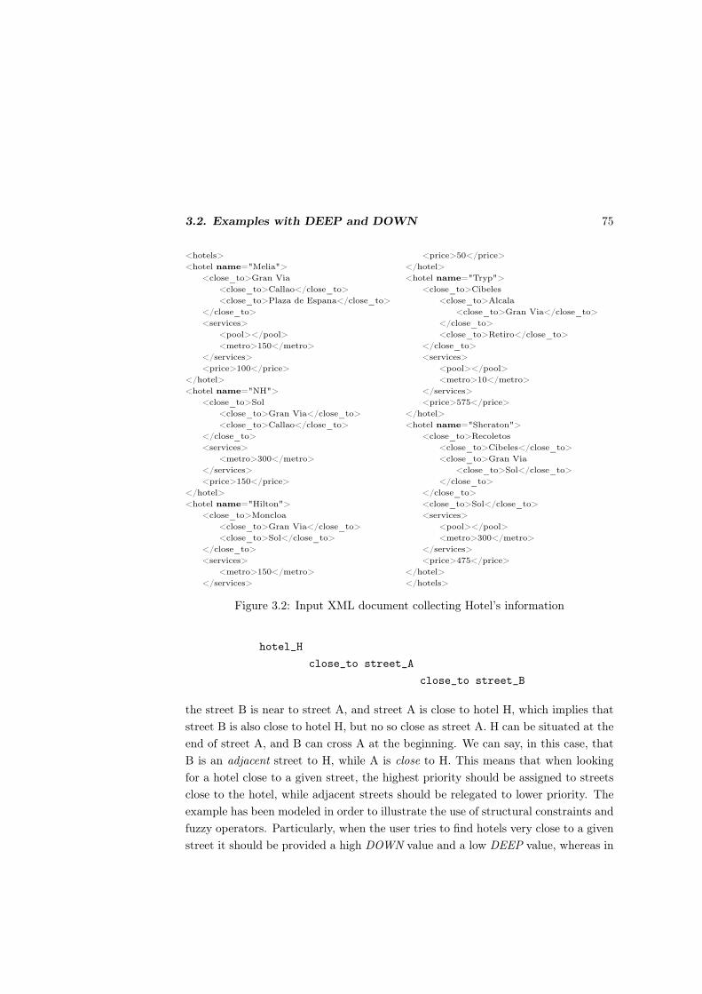
3.2. Examples with DEEP and DOWN 75
<hotels>
<hotel name="Melia">
<close_to>Gran Via
<close_to>Callao</close_to>
<close_to>Plaza de Espana</close_to>
</close_to>
<services>
<pool></pool>
<metro>150</metro>
</services>
<price>100</price>
</hotel>
<hotel name="NH">
<close_to>Sol
<close_to>Gran Via</close_to>
<close_to>Callao</close_to>
</close_to>
<services>
<metro>300</metro>
</services>
<price>150</price>
</hotel>
<hotel name="Hilton">
<close_to>Moncloa
<close_to>Gran Via</close_to>
<close_to>Sol</close_to>
</close_to>
<services>
<metro>150</metro>
</services>
<price>50</price>
</hotel>
<hotel name="Tryp">
<close_to>Cibeles
<close_to>Alcala
<close_to>Gran Via</close_to>
</close_to>
<close_to>Retiro</close_to>
</close_to>
<services>
<pool></pool>
<metro>10</metro>
</services>
<price>575</price>
</hotel>
<hotel name="Sheraton">
<close_to>Recoletos
<close_to>Cibeles</close_to>
<close_to>Gran Via
<close_to>Sol</close_to>
</close_to>
</close_to>
<close_to>Sol</close_to>
<services>
<pool></pool>
<metro>300</metro>
</services>
<price>475</price>
</hotel>
</hotels>
Figure 3.2: Input XML document collecting Hotel’s information
hotel_H
close_to street_A
close_to street_B
the street B is near to street A, and street A is close to hotel H, which implies that
street B is also close to hotel H, but no so close as street A. H can be situated at the
end of street A, and B can cross A at the beginning. We can say, in this case, that
B is an adjacent street to H, while A is close to H. This means that when looking
for a hotel close to a given street, the highest priority should be assigned to streets
close to the hotel, while adjacent streets should be relegated to lower priority. The
example has been modeled in order to illustrate the use of structural constraints and
fuzzy operators. Particularly, when the user tries to find hotels very close to a given
street it should be provided a high DOWN value and a low DEEP value, whereas in
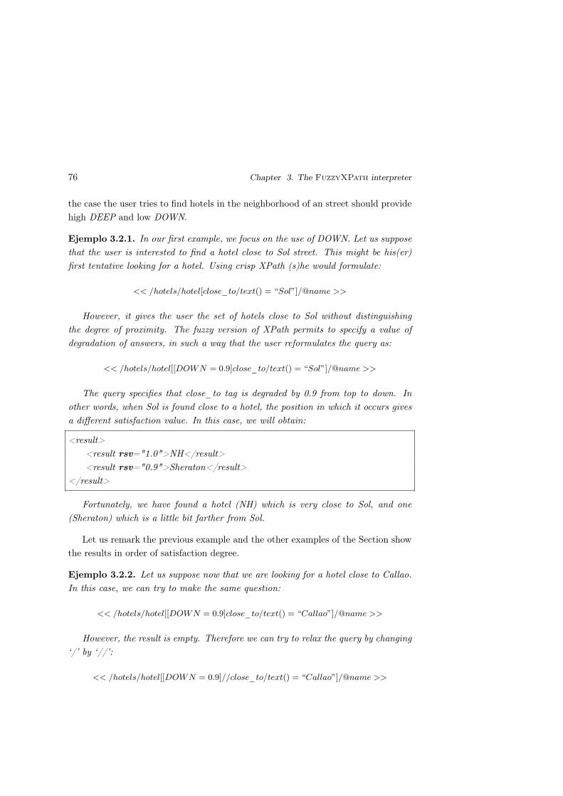
76 Chapter 3. The FuzzyXPath interpreter
the case the user tries to find hotels in the neighborhood of an street should provide
high DEEP and low DOWN.
Ejemplo 3.2.1. In our first example, we focus on the use of DOWN. Let us suppose
that the user is interested to find a hotel close to Sol street. This might be his(er)
first tentative looking for a hotel. Using crisp XPath (s)he would formulate:
<< /hotels/hotel[close_to/text() = “Sol”]/@name >>
However, it gives the user the set of hotels close to Sol without distinguishing
the degree of proximity. The fuzzy version of XPath permits to specify a value of
degradation of answers, in such a way that the user reformulates the query as:
<< /hotels/hotel[[DOWN = 0.9]close_to/text() = “Sol”]/@name >>
The query specifies that close_to tag is degraded by 0.9 from top to down. In
other words, when Sol is found close to a hotel, the position in which it occurs gives
a different satisfaction value. In this case, we will obtain:
<result>
<result rsv="1.0">NH</result>
<result rsv="0.9">Sheraton</result>
</result>
Fortunately, we have found a hotel (NH) which is very close to Sol, and one
(Sheraton) which is a little bit farther from Sol.
Let us remark the previous example and the other examples of the Section show
the results in order of satisfaction degree.
Ejemplo 3.2.2. Let us suppose now that we are looking for a hotel close to Callao.
In this case, we can try to make the same question:
<< /hotels/hotel[[DOWN = 0.9]close_to/text() = “Callao”]/@name >>
However, the result is empty. Therefore we can try to relax the query by changing
‘/’ by ‘//’:
<< /hotels/hotel[[DOWN = 0.9]//close_to/text() = “Callao”]/@name >>

3.2. Examples with DEEP and DOWN 77
Now, we will find answers, however, we will not be able to distinguish the prox-
imity of the hotels. Our fuzzy version of XPath permits to specify how the solutions
are degraded but not only taking into account the order but also the deepness. In
other words, there would be useful to give different weights to be a close street, and
to be an adjacent street. Therefore we can use the query:
<< /hotels/hotel[[DEEP = 0.5;DOWN = 0.9]//close_to/text() = “Callao”]/@name >>
obtaining the following results:
<result>
<result rsv="0.5">Melia</result>
<result rsv="0.45">NH</result>
</result>
It seems that Melia is near to Callao, and NH is a little bit farther than Melia.
Ejemplo 3.2.3. The use of DEEP combined with DOWN could be considered as the
best choice. However, DEEP can be used alone when the user only wants to penalize
adjacency. If we like to search hotels near to Gran Via street, degrading adjacent
streets with a factor of 0.5, we can consider the following query (and we obtain the
following result):
<< //hotel[[DEEP = 0.5]//close_to/text() = “GranV ia”]/@name >>
<result>
<result rsv="1.0">Melia</result>
<result rsv="0.5">NH</result>
<result rsv="0.5">Hilton</result>
<result rsv="0.5">Sheraton</result>
<result rsv="0.25">Tryp</result>
</result>
We can see that Melia is close to Gran Via, while NH, Hilton and Sheraton are
situated in adjacent streets of Gran Via. Tryp is the farthest hotel.
Ejemplo 3.2.4. The following table summarizes the results by combining DEEP
and DOWN in a single query:

78 Chapter 3. The FuzzyXPath interpreter
<< //hotel[[DEEP = r1;DOWN = r2]//close_to/text() = “GranV ia”]/@name >>
HOTEL (A: r1 = 0.1, r2 = 1) (B: r1 = 0.5, r2 = 0.5) (C: r1 = 1, r2 = 0.1)
Melia
NH
Hilton
Tryp
Sheraton
1
0.1
0.1
0.01
0.1
1
0.5
0.5
0.25
0.25
1
1
1
1
0.1
While case C only penalizes closeness, case A penalizes adjacency. Case B pe-
nalizes both closeness and adjacency.
3.3 AVG Examples
Ejemplo 3.3.1. Let us suppose that the user is interested in a hotel combining two
services like pool and metro. Instead of using classical and/or connectives for mixing
both features, we can obtain more flexible estimations on RSV values by using the
avg operator as follows:
<< //hotel[services/pool avg services/metro]/@name >>
thus obtaining the following results:
<result>
<result rsv="1.0">Melia</result>
<result rsv="1.0">Tryp</result>
<result rsv="1.0">Sheraton</result>
<result rsv="0.5">NH</result>
<result rsv="0.5">Hilton</result>
</result>
By using the avg fuzzy operator, the user finds that Melia, Tryp and Sheraton
have pool and metro, while NH and Hilton lack on one of them.
Ejemplo 3.3.2. Now, let us suppose that the importance of the metro is the double
of the importance of the pool. In this case, the user can formulate the query as
follows:

3.3. AVG Examples 79
<< //hotel[services/pool avg1, 2 services/metro]/@name >>
obtaining the following results:
<result>
<result rsv="1.0">Melia</result>
<result rsv="1.0">Tryp</result>
<result rsv="1.0">Sheraton</result>
<result rsv="0.666667">NH</result>
<result rsv="0.666667">Hilton</result>
</result>
We can see in the results that NH and Hilton increase the degree of satisfaction
w.r.t. the previous query given that they have metro station.
Ejemplo 3.3.3. Let us suppose the user is looking now for hotels giving more im-
portance to the fact that the price of the hotel is lower than 150 euros than to the
proximity to Sol street. The user can formulate the query as follows, obtaining the
results below:
<< //hotel[[DEEP = 0.8]//close_to/text() = “Sol” avg1, 2 //price/text() < 150]/@name >>
<result>
<result rsv="0.933333">Hilton</result>
<result rsv="0.666667">Melia</result>
<result rsv="0.333333">NH</result>
<result rsv="0.333333">Sheraton</result>
</result>
Now, we take a new input XML document, Figure 3.3, whose skeleton is depicted
in Figure 3.4 that will help us better understand the AVG operator, this document
represents a collection of books; all results of this document will be accompanied by
table showing the calculation performed for RSV.
Ejemplo 3.3.4. The Figure 3.5 shows the answer associated to the XPath expres-
sion:
<< /bib/book[@price < 30 avg @year < 2006] >>

80 Chapter 3. The FuzzyXPath interpreter
<bib>
<book year="2001" price="45.95">
<title>Don Quijote de la Mancha</title>
<author>Miguel de Cervantes Saavedra</author>
<publications> <book year="1997" price="35.99">
<title>La Galatea</title>
<author>Miguel de Cervantes Saavedra</author>
<publications>
<book year="1994" price="25.99">
<title>Los trabajos de Persiles y Segismunda</title>
<author>Miguel de Cervantes Saavedra</author></book>
</publications></book>
</publications></book>
<book year="1999" price="25.65">
<title>La Celestina</title>
<author>Fernando de Rojas</author></book>
<book year="2005" price="29.95">
<title>Hamlet</title>
<author>William Shakespeare</author>
<publications>
<book year="2000" price="22.5">
<title>Romeo y Julieta</title>
<author>William Shakespeare</author></book>
</publications></book>
<book year="2007" price="22.95">
<title>Las ferias de Madrid</title>
<author>Felix Lope de Vega y Carpio</author>
<publications>
<book year="1996" price="27.5">
<title>El remedio en la desdicha</title>
<author>Felix Lope de Vega y Carpio</author> </book>
<book year="1998" price="12.5">
<title>La Dragontea</title>
<author>Felix Lope de Vega y Carpio</author></book>
</publications></book>
</bib>
Figure 3.3: Input XML document collecting books
Figure 3.4: XML document collecting books represented as a tree.

3.4. Thresholding Example 81
Here we show that books satisfying a price under 30 and a year before 2006 have
the highest RSV.
Document RSV computation
<result>
<book rsv="0.5" ...> <title>Don Quijote ...</title> ...</book>
<book rsv="1.0"...><title>La Celestina</title> ...</book>
<book rsv="1.0" ...><title>Hamlet</title> ...</book>
<book rsv="0.5" ...><title>Las ferias de Madrid</title> ...</book>
</result>
0.5 = (0 + 1)/2
1 = (1 + 1)/2
1 = (1 + 1)/2
0.5 = (1 + 0)/2
Figure 3.5: Output of a query using the average operator AVG
Ejemplo 3.3.5. Finally, in Figure 3.6 we combine all operators (thus obtaining
more scattered RSV values) in query:
«[DEEP=0.9,DOWN=0.8]//book[(@price>25 and @price<30) avg (@year<2000 or @year>2006)]/title»
Document RSV computation
<result>
<title rsv="0.3645">La Galatea</title>
<title rsv="0.59049">Los trabajos de Persiles y Si...</title>
<title rsv="0.72">La Celestina</title>
<title rsv="0.288">Hamlet</title>
<title rsv="0.2304">Las ferias de Madrid</title>
<title rsv="0.373248">El remedio en la desdicha</title>
<title rsv="0.149299">La Dragontea</title>
</result>
0.3645 = 0.93 ∗ 1/2
0.59049 = 0.95 ∗ 1
0.72 = 0.9 ∗ 0.8 ∗ 1
0.288 = 0.9 ∗ 0.82 ∗ 1/2
0.2304 = 0.9 ∗ 0.83 ∗ 1/2
0.373248 = 0.93 ∗ 0.83 ∗ 1
0.149299 = 0.93 ∗ 0.84 ∗ 1/2
Figure 3.6: Output of a query using all operators
3.4 Thresholding Example
Fuzzy conditions return a satisfaction degree in the infinite space of real numbers
between 0 and 1. We can take profit of this feature by imposing thresholds to such
conditions, thus filtering the set of solutions according to the satisfaction degree. The
idea is to formulate queries by directly acting on the satisfaction degrees obtained
after evaluating “fuzzy” conditions.
Ejemplo 3.4.1. For instance, let us suppose that in the query of example 3.2.3, the
user looks for hotels in which the degree of proximity to Gran Via street is greater

82 Chapter 3. The FuzzyXPath interpreter
than seventy five per cent (i.e., value 0.75 measured between 0 and 1) then (s)he can
formulate the following query, obtaining the following results:
<< //hotel[([DEEP = 0.5]//close_to/text() = “Gran V ia”) > 0.75]/@name >>
<result>
<result rsv="1.0">Melia</result>
</result>
3.5 Conjunctive/Disjunctive Connective Examples
Ejemplo 3.5.1. In the following queries we express the following requirement: hotels
near to Gran Via, near to a metro station, having pool, with greater preference (3 to
2) to pool than metro. We will use and+, and and and- which provide distinct levels
of exigency, which are demonstrated in the results.
<< //hotel[([DEEP = 0.5]//close_to/text() = ”GranV ia”) and+ (//pool avg3, 2 //metro/text() < 200)]/@name >>
<result>
<result rsv="1.0">Melia</result>
<result rsv="0.5">Sheraton</result>
<result rsv="0.4">Hilton</result>
<result rsv="0.25">Tryp</result>
</result>
<< //hotel[([DEEP = 0.5]//close_to/text() = ”GranV ia”) and (//pool avg3, 2 //metro/text() < 200)]/@name >>
<result>
<result rsv="1.0">Melia</result>
<result rsv="0.3">Sheraton</result>
<result rsv="0.25">Tryp</result>
<result rsv="0.2">Hilton</result>
</result>

3.6. Dynamic Filtering for Improving Efficiency 83
<< //hotel[([DEEP = 0.5]//close_to/text() = ”GranV ia”) and− (//pool avg3, 2 //metro/text() < 200)]/@name >>
<result>
<result rsv="1.0">Melia</result>
<result rsv="0.25">Tryp</result>
<result rsv="0.1">Sheraton</result>
</result>
So, in the first case (the least demanding and optimistic) we obtain four hotels
(Melia, Sheraton, Hilton and Tryp), as well as in the second case (a little bit more
exigent) while third table (the strongest one) lists three candidates (Melia, Tryp and
Sheraton). Sheraton and Hilton are degraded using and and and-. This effect would
even be more evident when previous conditions are compared with a threshold. For
instance, to be greater than 0.25. In such a case and- gives just a single solution:
Melia.
3.6 Dynamic Filtering for Improving Efficiency
In [JMMO10, JMM+13] we have reported some thresholding techniques specially
tailored for the MALP language, where the main idea consists in to dynamically
create and evaluate filters for prematurely disregarding those superfluous computa-
tions leading to non-significant solutions. Somehow inspired by the same guidelines,
we have recently equipped our FuzzyXPath interpreter with a command with syn-
tax «[FILTER=r]» (being r a real number between 0 and 1) which can be used just
at the beginning of a query for indicating that only those answers with RSV greater
of equal than r must be generated and reported. As we have described in [ALM14a],
when «[FILTER=r]» precedes a fuzzy query, the interpreter lazily explores an input
XML document for dynamically disregarding as soon as possible those branches of
the XML tree leading to irrelevant solutions with an RSV degraded below r, thus
allowing the possibility of efficiently managing large files without reducing the set
of answers for which users are mainly interested in.
In order to explain the benefits of using the FILTER command, let us consider
in this section the XML document shown in Figure 3.3, for which the execution of
query,
<< [//book[@year < 2000 avg @price < 50]/title >>

84 Chapter 3. The FuzzyXPath interpreter
produces the following set of solutions:
<result>
<title rsv="1.0">La Galatea</title>
<title rsv="1.0">Los trabajos de Persiles y Sigismunda</title>
<title rsv="1.0">La Celestina</title>
<title rsv="1.0">El remedio en la desdicha</title>
<title rsv="1.0">La Dragontea</title>
<title rsv="0.5">Don Quijote de la Mancha</title>
<title rsv="0.5">Hamlet</title>
<title rsv="0.5">Romeo y Julieta</title>
<title rsv="0.5">Las ferias de Madrid</title>
</result>
If we consider now the new, quite similar query «[FILTER=0.4]//book[@year <2000
avg @price<50]/title», we clearly obtain again nine answers, but only five if we
fix «[FILTER=0.8]». Obviously, we would hope that the runtime of the second
case should be lower than the first one since, as our approach does, there is no
need for computing all solutions and then filtering the best ones. This desired
dynamic behaviour when avoiding useless computations is reflected in Figure 3.7
which considers the effort needed for executing (excluding parsing/compiling time)
a query like,
<< [FILTER = r]//book[(@price > 25 and @price < 30) avg (@year < 2000 or @year > 2006)] >>
where each row represents the size of several XML files accomplishing with the same
structure of our running example (but considering different nesting levels of tags
book, title, author and publications), and each column refers to a different degree of
the FILTER command. Here, the runtime is measured in seconds (the benchmarks
have been performed using a computer with processor Intel Core Duo, with 2 GB
RAM and Windows Vista) and each record in the input file refers to a different book
(that is, the number of records coincides with the number of occurrences of tag book)
which might contain other books inside its publications tag.
Moreover, in Figure 3.8 we continue with a similar query to the previous one,
but also considering the DEEP command2. Here, for a large XML document with
2This kind of statistics can be produced on-line for several XML files and FuzzyXPath queries
via the following URL that we have just prepared for the interested reader: http://http://dectau.
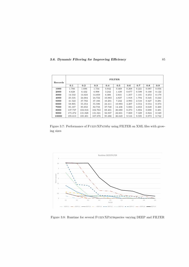
3.6. Dynamic Filtering for Improving Efficiency 85
Records
FILTER
0.1 0.2 0.3 0.4 0.5 0.6 0.7 0.8 0.9
1000 1.766 1.696 1.734 0.842 0.469 0.268 0.221 0.087 0.056
2000 6.628 6.432 6.998 3.242 1.439 0.677 0.599 0.168 0.122
3000 14.532 14.023 14.059 6.306 2.831 1.257 1.101 0.253 0.179
4000 25.535 24.684 24.722 10.883 4.827 1.918 1.794 0.345 0.242
5000 41.522 37.782 37.166 16.201 7.242 2.993 2.516 0.427 0.281
6000 58.905 55.354 55.596 24.411 10.993 4.207 3.554 0.554 0.373
7000 85.167 85.652 82.733 37.748 14.436 5.083 4.653 0.649 0.460
8000 137.737 102.816 102.763 69.401 26.680 8.273 5.894 0.690 0.481
9000 175.272 131.828 131.021 56.937 22.601 7.869 7.329 0.824 0.549
10000 195.613 185.201 167.676 95.286 26.649 9.516 9.595 0.973 0.742
Figure 3.7: Performance of FuzzyXPathby using FILTER on XML files with grow-
ing sizes
0
0,5
1
1,5
2
2,5
3
3,5
4
0,1 0,2 0,3 0,4 0,5 0,6 0,7 0,8 0,9
Tim
e i
n s
eco
nd
FILTER
Run e DEEP/FILTER
DEEP 0.1 DEEP 0.2 DEEP 0.3 DEEP 0.4 DEEP 0.5 DEEP 0.6 DEEP 0.7 DEEP 0.8 DEEP 0.9
Figure 3.8: Runtime for several FuzzyXPathqueries varying DEEP and FILTER

86 Chapter 3. The FuzzyXPath interpreter
0
0,2
0,4
0,6
0,8
1
1,2
1,4
1,6
1,8
0,1 0,2 0,3 0,4 0,5 0,6 0,7 0,8 0,9
Tim
e i
n s
eco
nd
FILTER
Run e DEEP/FILTER
DEEP 0.1 DEEP 0.2 DEEP 0.3 DEEP 0.4 DEEP 0.5 DEEP 0.6 DEEP 0.7 DEEP 0.8 DEEP 0.9
Figure 3.9: Varying DEEP and FILTER in a query using avg30, 1
0
0,5
1
1,5
2
2,5
3
3,5
0,1 0,2 0,3 0,4 0,5 0,6 0,7 0,8 0,9
Tim
e i
n s
eco
nd
FILTER
Run e DEEP/FILTER
DEEP 0.1 DEEP 0.2 DEEP 0.3 DEEP 0.4 DEEP 0.5 DEEP 0.6 DEEP 0.7 DEEP 0.8 DEEP 0.9
Figure 3.10: Varying DEEP and FILTER in a query using avg1, 30

3.6. Dynamic Filtering for Improving Efficiency 87
[element(bib,[],
[element(book,[year=2001,price=45.95],
[element(title,[],[Don Quijote de la Mancha]),
element(author,[],[Miguel de Cervantes Saavedra]),
element(publications,[],
[element(book,[year=1997,price=35.99],
[element(title,[],[La Galatea]),
element(author,[],[Miguel de Cervantes Saavedra]),
element(publications,[],...])...]),])])
Figure 3.11: A data-term representing a XML document
a fixed size, we express the number of seconds needed for executing such query
when varying FILTER and DEEP, where it is easy to see that the behaviour is
more and more improved whenever FILTER grows and DEEP decreases, as wanted.
Note that the previous query makes use of the avg command and remember that
its behaviour is defined, for two given RSV’s r1 and r2, as r3 = (r1 + r2)/2, we
can now use the priorized version of such operator which let us to give different
degrees of importance to its arguments (remember that, for two given RSV’s r1 and
r2, avgp1, p2 is computed by r3 = (r1 ∗ p1 + r2 ∗ p2)/(p1 + p2)) and hence, if in
the previous query we use avg30, 1 instead of standard avg, we indicate that the
first sub-condition (i.e., @price>25 and @price<30) is 30 times more important than
the second one (i.e., @year<2000 or @year>2006), whereas avg1, 30 represent the
inverse criterion. In Figures 3.9 and 3.10 we provide statistics in the same way than
in Figure 3.8, but using now average with priorities 30-1 and 1-30, respectively.
Although the core of our application is written with (fuzzy) MALP rules, our
implementation is based on the following items:
(1) We have reused/adapted several modules of our previous −based implementa-
tion of (crisp) XPath described in [Alm09, ABE08].
(2) We have used the SWI- library for loading XML files, in order to represent a
XML document by means of a term3.
(3) The parser of XPath has been extended to recognize the new keywords FILTER,
DEEP, DOWN, avg, etc... with their proper arguments.
uclm.es/fuzzyXPath/?q=FuzzyXPathStatistics.3The notion of term (i.e., data structure) is just the same in MALP and .

88 Chapter 3. The FuzzyXPath interpreter
(4) Each tag is represented as a data-term of the form: element(Tag, Attri-
butes, Subelements), where Tag is the name of the XML tag, Attributes
is a list containing the attributes, and Subelements is a list containing the
sub-elements (i.e. sub-trees) of the tag. For instance, the document of Fig-
ure 3.3 is represented in SWI- like in Figure 3.11. Loading of documents
is achieved by predicate load_xml(+File,-Term) and writing by predicate
write_xml(+File,+Term).
(5) Predicate fuzzyXPath(+ListXPath,+Tree,+Deep,+Down,+Filter,+Accum) re-
ceives six arguments: (1) ListXPath is the representation of a XPath ex-
pression; (2) Tree is the term representing an input XML document; (3)
Deep/Down/Filter have the obvious meaning, and finally (4) the last argu-
ment Accum (which is appropriately updated -maybe decreased- when going
deeper in the exploration of the file) accumulates the sequence of penalties
produced till reaching a concrete node, and it is very useful for deciding when
performing a recursive call to the children of such node whenever the value of
Accum is better than the one fixed by Filter.
tv(1, [[],
tv(0.9,[[],
tv(0.9,[element(title,[],[Don Quijote de la Mancha]),[],
tv(1,[[],[],
tv(1,[[],
tv(0.9,[[],
tv(0.9,[element(title,[],[La Galatea]),[],
tv(1,[[],[],
tv(1,[[],
tv(0.9,[[],
tv(0.9,[element(title,[],[Los trabajos de Persiles..]),...]),
tv(0.8,[[],
tv(0.9,[element(title,[],[La Celestina]),[],[]]),...
Figure 3.12: Example of a MALP output
(6) The evaluation of the query generates a truth value which has the form of a
tree, called tv tree. For instance, the query << [DEEP = 0.9, DOWN =
0.8]//title >> generates the one illustrated in Figure 3.12. The main power
of a fuzzy logic programming language like MALP w.r.t. , is that instead of
answering questions with a simple true/false value, solutions are reported in
a much more tinged, documented way. Basically, the FuzzyXPath predicate
traverses the tree representing a XML document annotating into the tv tree

3.6. Dynamic Filtering for Improving Efficiency 89
the corresponding deep/down values according to the movements performed
in the horizontal and vertical axis, respectively. In addition, the tv tree is
annotated with the values of and, or and avg operators in each node.
(7) Finally, the tv tree is used for computing the output of the query, by multiplying
the recorded values. A predicate called tv_to_elem has been implemented to
output the answer in a pretty way.

90 Chapter 3. The FuzzyXPath interpreter
Chapter 4
Implementation Issues
User’s preferences play a key role in information retrieval. In modern Web based
information retrieval systems, user expects to introduce his(er) key words and pref-
erences to influence the search results. However, while the technology is still improv-
ing, users get sometimes frustrated with those retrieval systems which only offer a
poor/rigid set of expressive resources. Therefore the need for flexible query languages
arises, in which the user can formulate queries according to his(er) preferences, being
adaptable to data schema but without increasing complexity. In addition, flexible
query languages should be equipped with a mechanism for obtaining a certain ranked
list of answers. The ranking of answers can provide satisfaction degrees depending
on several factors.
The XPath language [BBC+07] has been proposed as a standard for XML query-
ing and it is based on the description of the path in the XML tree to be retrieved.
XPath allows to specify the name of nodes (i.e., tags) and attributes to be present
in the XML tree together with boolean conditions about the content of nodes and
attributes.
XPath querying mechanism is based on a boolean logic: the nodes retrieved
from an XPath expression are those matching the path of the XML tree. Therefore,
the user should know the XML schema in order to specify queries. However, even
when the XML schema exists, it may not be available for users. Moreover, XML
documents with the same XML schema can be very different in structure. Let us
suppose the case of XML documents containing the curriculum vitae of a certain
group of persons. Although they can share the same schema, each one can decide to
91

92 Chapter 4. Implementation Issues
include studies, jobs, training, etc. organized in several ways: by year, by relevance,
and with different nesting degree. In an XPath-based structural query, the main
criteria to provide a certain degree of satisfaction are the hierarchical deepness and
document order. However, user’s preferences play also a key role in determining the
best solutions. Conditions on XPath expressions are usually of varying importance
for a user, that is, the user gives a higher degree of importance to certain require-
ments when satisfying his(er) wishes. Therefore, the query language should provide
mechanisms for assigning priority to answers, when they occur in different parts of
the document, as well as priority to queries, with regard to user’s preferences.
4.1 Multi-Adjoint Logic Programming and FuzzyX-
Path
In this section, we will introduce the elements of multi-adjoint logic programming
(MALP). MALP will serve as semantic foundation of our proposal. Moreover, MALP
will be used for the implementation of our language. The section will describe the
theoretical basis of MALP: multi-adjoint lattices and fuzzy operators defined on
them. In addition, it will be described an instance of MALP which considers a
multi-adjoint lattice of trees with truth values, and operators defined for such lattice.
Finally, we will describe the rule-based implementation of our FuzzyXPath by using
MALP rules.
4.1.1 Multi-Adjoint Logic Programming
In multi-adjoint logic programming [MOV04, JMP09], we work with a first or-
der language, L, containing variables, function symbols, predicate symbols, con-
stants, quantifiers (∀ and ∃), and several arbitrary connectives such as implications
(←1,←2, . . . ,←m), conjunctions (&1,&2, . . . ,&k), disjunctions (∨1,∨2, . . . ,∨l), and
general hybrid operators (“aggregators” @1,@2, . . . ,@n), used for combining/propa-
gating truth values through the rules, and thus increasing the language expressive-
ness. Additionally, our language L contains symbols called truth degrees belonging
to a multi-adjoint lattice L, whose formal description will be presented afterward in
Definition 4.1.5 (see also Figure 4.2).
A rule is a formula “A ←i B with α”, where A is an atomic formula (usually
called the head), B (which is called the body) is a formula built from atomic formulas

4.1. Multi-Adjoint Logic Programming and FuzzyXPath 93
B1, . . . , Bn (n ≥ 0 ), truth values of L and conjunctions, disjunctions and general
aggregations, and finally α ∈ L is the “weight” or truth degree of the rule. The set of
truth values L may be the carrier of any complete lattice, as for instance occurs with
the interval ([0, 1],≤), where ≤ is the usual order. Consider, for instance, the pro-
gram P of Figure 4.1 composed of three rules with associated multi-adjoint lattice
〈[0, 1],≤,←P,&P〉, where label P stands for Product logic with the following connec-
tive definitions (for implication, conjunction and disjunction symbols, respectively):
“←P (x, y) = min(1, x/y)”, “&P(x, y) = x ∗ y” and “ |P(x, y) = x+ y − x ∗ y”.
R1 : p(X) ←P q(X,Y ) |P r(Y ) with 0.8
R2 : q(a, Y ) ← with 0.9
R3 : r(b) ← with 0.7
Figure 4.1: Example of MALP program
In order to describe the procedural semantics of the multi–adjoint logic language,
in the following we denote by C[A] a formula where A is a sub-expression (usually an
atom) which occurs in the –possibly empty– one hole context C[] whereas C[A/A′]
means the replacement of A by A′ in context C[], and mgu(E) is the most general
unifier of an equation set E. The pair 〈Q;σ〉 composed of a goal and a substitution
is called a state. So, given a program P, an admissible computation is formalized
as a state transition system, whose transition relation →AS is the smallest relation
satisfying the following admissible rules:
1) 〈Q[A];σ〉→AS〈(Q[A/v&iB])θ;σθ〉 if A is the selected atom in goal Q,
A′←iB with v in P, where B is not empty, and θ = mgu(A′ = A)
2) 〈Q[A];σ〉→AS〈(Q[A/v])θ;σθ〉 if A′← with v in P, θ = mgu(A′ = A)
The following derivation illustrates our definition (note that the exact program rule
used -after being renamed, that is, standardized apart- in the corresponding step is
annotated as a super–index symbol, whereas exploited atoms appear underlined):
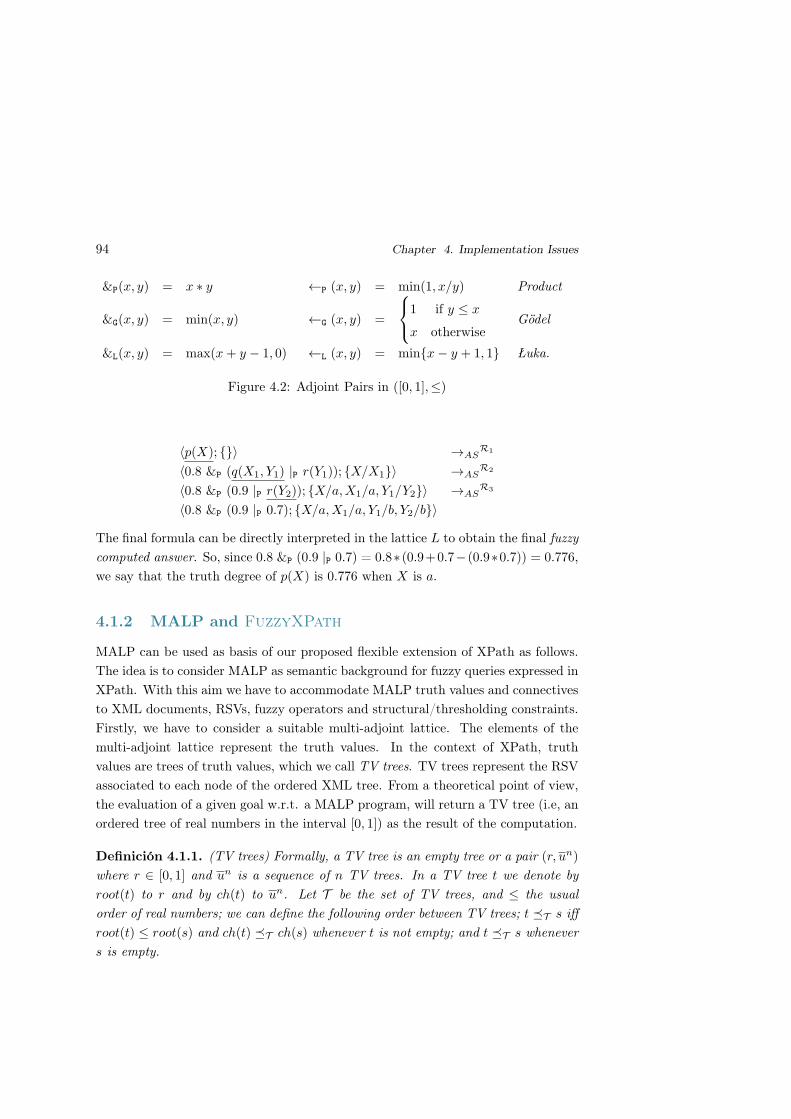
94 Chapter 4. Implementation Issues
&P(x, y) = x ∗ y ←P (x, y) = min(1, x/y) Product
&G(x, y) = min(x, y) ←G (x, y) =
1 if y ≤ x
x otherwiseGödel
&L(x, y) = max(x+ y − 1, 0) ←L (x, y) = minx− y + 1, 1 Łuka.
Figure 4.2: Adjoint Pairs in ([0, 1],≤)
〈p(X); 〉 →ASR1
〈0.8 &P (q(X1, Y1) |P r(Y1)); X/X1〉 →ASR2
〈0.8 &P (0.9 |P r(Y2)); X/a,X1/a, Y1/Y2〉 →ASR3
〈0.8 &P (0.9 |P 0.7); X/a,X1/a, Y1/b, Y2/b〉
The final formula can be directly interpreted in the lattice L to obtain the final fuzzy
computed answer. So, since 0.8 &P (0.9 |P 0.7) = 0.8∗ (0.9+0.7− (0.9∗0.7)) = 0.776,
we say that the truth degree of p(X) is 0.776 when X is a.
4.1.2 MALP and FuzzyXPath
MALP can be used as basis of our proposed flexible extension of XPath as follows.
The idea is to consider MALP as semantic background for fuzzy queries expressed in
XPath. With this aim we have to accommodate MALP truth values and connectives
to XML documents, RSVs, fuzzy operators and structural/thresholding constraints.
Firstly, we have to consider a suitable multi-adjoint lattice. The elements of the
multi-adjoint lattice represent the truth values. In the context of XPath, truth
values are trees of truth values, which we call TV trees. TV trees represent the RSV
associated to each node of the ordered XML tree. From a theoretical point of view,
the evaluation of a given goal w.r.t. a MALP program, will return a TV tree (i.e, an
ordered tree of real numbers in the interval [0, 1]) as the result of the computation.
Definición 4.1.1. (TV trees) Formally, a TV tree is an empty tree or a pair (r, un)
where r ∈ [0, 1] and un is a sequence of n TV trees. In a TV tree t we denote by
root(t) to r and by ch(t) to un. Let T be the set of TV trees, and ≤ the usual
order of real numbers; we can define the following order between TV trees; t T s iff
root(t) ≤ root(s) and ch(t) T ch(s) whenever t is not empty; and t T s whenever
s is empty.

4.1. Multi-Adjoint Logic Programming and FuzzyXPath 95
!!!"#$!
!!!"#%! !!!"#$! !!!"#&!
!!!"#'! !!!"#(! !!!"#)!
!!!"#%!
!!!"#%! !!!"#*!
!!!"#(!
Figure 4.3: TV trees partial order
Abusing from the notation, in the previous T is used for sequences of TV trees,
whose definition is as follows. Given two sequences of TV trees un = (u1, . . . , un)
and vm = (v1, . . . , vm) then un T vm whenever there exists a subsequence sm of
un such that si T vi for all 1 ≤ i ≤ m.
Intuitively, TV trees are ordered in decreasing order w.r.t. size, and increasing
w.r.t. the relation on real numbers, and therefore the biggest element is the empty
tree. We can see in Figure 4.3 an example of trees ordered by the T relation, where
the sequence of children is ((0.7, (0.5)), (0.6, (0.4, 0.8))); an alternative sequence is
(0.3, (0.6, (0.4, 0.8))).
We denote by first(un, k) (resp. last(un, k)) the first n−k (resp. last k) elements
of the sequence un. When k > n then first(un, k) is completed with k-n empty trees
at the right hand side and last(un, k) is completed with k-n empty trees at the left
hand side.
Proposición 4.1.2. T is a partial order (reflexive, antisymmetric and transitive).
Proof. Reflexivity and transitivity can be easily proved. The relation is antisym-
metric reasoning by induction as follows. Let us suppose t T s and s T t
then, when t and s are empty then trivially s = t; otherwise root(t) ≤ root(s)
and root(s) ≤ root(t) therefore root(t) = root(s); in addition (a) there exists a
subsequence sm of un such that sj T wi, 1 ≤ i ≤ m, where ch(t) = un and
ch(s) = wm; analogously, (b) there exists a subsequence ln
of wm of such that
lk T uk, 1 ≤ k ≤ n. We can reason now that n = m: from (a) we have that
n ≥ m, and from (b) we have that m ≥ n. Now, from (a) un T wn and from (b)
wn T un, thus by hypothesis un = wn, and therefore s = t.
Now, we can define the following operations in the set T .
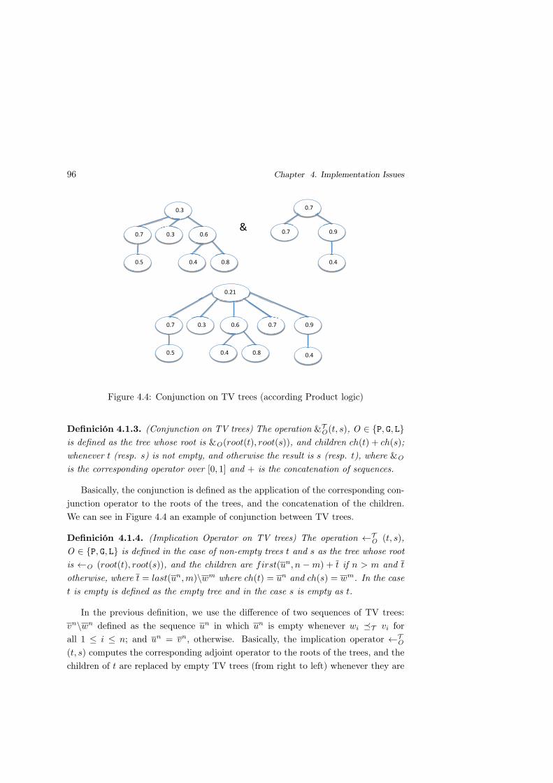
96 Chapter 4. Implementation Issues
!!!"#$!
!!!"#%! !!!"#$! !!!"#&!
!!!"#'! !!!"#(! !!!"#)!
!!!"#%!
!!!"#%! !!!"#*!
!!!"#(!
!!!"#+,!
!!!"#%! !!!"#$! !!!"#&!
!!!"#'! !!!"#(! !!!"#)!
!!!"#%! !!!"#*!
!!!"#(!
-!
Figure 4.4: Conjunction on TV trees (according Product logic)
Definición 4.1.3. (Conjunction on TV trees) The operation &TO(t, s), O ∈ P, G, L
is defined as the tree whose root is &O(root(t), root(s)), and children ch(t) + ch(s);
whenever t (resp. s) is not empty, and otherwise the result is s (resp. t), where &O
is the corresponding operator over [0, 1] and + is the concatenation of sequences.
Basically, the conjunction is defined as the application of the corresponding con-
junction operator to the roots of the trees, and the concatenation of the children.
We can see in Figure 4.4 an example of conjunction between TV trees.
Definición 4.1.4. (Implication Operator on TV trees) The operation ←TO
(t, s),
O ∈ P, G, L is defined in the case of non-empty trees t and s as the tree whose root
is ←O (root(t), root(s)), and the children are first(un, n −m) + t if n > m and t
otherwise, where t = last(un,m)\wm where ch(t) = un and ch(s) = wm. In the case
t is empty is defined as the empty tree and in the case s is empty as t.
In the previous definition, we use the difference of two sequences of TV trees:
vn\wn defined as the sequence un in which un is empty whenever wi T vi for
all 1 ≤ i ≤ n; and un = vn, otherwise. Basically, the implication operator ←TO
(t, s) computes the corresponding adjoint operator to the roots of the trees, and the
children of t are replaced by empty TV trees (from right to left) whenever they are

4.1. Multi-Adjoint Logic Programming and FuzzyXPath 97
0.8
0.7 0.7 0.6
0.5 0.4 0.8
0.2
0.6 0.5
0.4
ßP
0.25
0.7
0.5
Figure 4.5: Implication on TV trees (according Product logic)
greater or equal than the corresponding element of s. We can see in Figure 4.5 an
example of use of the implication, in the case of product logic, between TV trees.
Our goal now is to prove that TV trees conform a multi-adjoint lattice defined
as follows.
Definición 4.1.5. Let (L,) be a lattice. A multi-adjoint lattice is a tuple:
〈L,,←1 ,&1 , . . . ,←n ,&n〉
such that:
1. (L,) is complete, namely, ∀S ⊂ L non empty ∃inf(S), sup(S). Then, it is
a bounded lattice, i.e. it has bottom and top elements, denoted by ⊤ and ⊥,
respectively.
2. (&i,←i) is an adjoint pair in (L,), i.e.:
(a) &i is non decreasing in both arguments, for all i, i = 1, . . . , n.
(b) ←i is non decreasing in the first argument and non increasing in the
second, for all i.
(c) x (y←iz) if and only if (x&iz) y, for any x, y, z ∈ L (adjoint
property).

98 Chapter 4. Implementation Issues
3. ⊤&iv = v&i⊤ = v for all v ∈ L, i = 1, . . . , n, where ⊤ = sup(L).
TV trees are a multi-adjoint lattice based on truth values over [0, 1]. In order to
prove this property, we need the following auxiliary proposition.
Proposición 4.1.6. 〈[0, 1],≤,←P,&P,←G,&G,←L,&L〉 is a multi-adjoint lattice.
Note that even when the previous claim holds too for many other arbitrary multi-
adjoint lattices (L,), we prefer to accommodate it to the [0, 1] case because our
notion of TV trees simply relies on this concrete kind of basic truth degrees (i.e., real
numbers in the unit interval). Now, we are ready to establish the following theorem
proving our intended result.
Teorema 4.1.7. 〈T ,T ,←TP ,&
TP ,←T
G ,&TG ,←T
L ,&TL 〉 is a multi-adjoint lattice.
Proof. 1. Let be a non empty S ⊂ T , then inf(S) is defined as the empty TV tree
whenever all the elements of S are empty, otherwise as the TV tree whose root
is the infimum of the roots of the non-empty elements of S, and the children
are the sequence un where ui = inf(wi|wn ∈ perm(s)n, s ∈ S), where n =
maxChildren(S) represents the maximum number of children of the elements
of S, and perm(s)n is the set of all sequences of length n including ch(s)
as subsequence and empty trees in the other positions. Now, inf(S) T s,
for all s ∈ S by construction: when s ∈ S then root(inf(S)) ≤ root(s) and
inf(wi|perm(s)n = wn, s ∈ S) T ch(s) given that ch(s) is a subsequence
of a sequence of perm(s). Now, inf(S) is the greatest lower bound: let us
suppose t T s for all s ∈ S; now, root(t) ≤ root(s) for all s ∈ S; thus
root(inf(S)) ≤ root(t); in addition ch(t) T ch(s) for all s ∈ S, and thus,
for all p ∈ perm(t)n and q ∈ perm(s)n we have that p T q; and then
inf(wi|wn ∈ perm(s)n, s ∈ S) T p T ch(t), concluding that inf(S) T t.
Analogously, sup(S) is defined as the empty TV tree whenever all the elements
of S are empty, otherwise as the TV tree whose root is the supremum of the
roots of the non-empty elements of S, and the children are the sequence un
where ui = sup(wi|wn ∈ perm(s)n, s ∈ S), where n = maxChildren(S). ⊤of T is the empty tree and ⊥ is the (infinite) tree with 0 in all nodes.
2. (a) &TO, O ∈ P, G, L is non decreasing: by Proposition 4.1.6 whenever v T
s, v′ T s′ then root(v)&Oroot(v′) ≤ root(s)&Oroot(s
′); in addition,
ci T bi, c′k T b′k, for subsequences cn of ap and c′m
of a′q, where
ch(v) = ap, ch(s) = bn, ch(v′) = a′
qand ch(s′) = b′
m. Now, the children

4.1. Multi-Adjoint Logic Programming and FuzzyXPath 99
of &TO(v, v
′) is ap + a′q, and the children of &T
O(s, s′) is b
n+ b′
m, thus
&TO(v, v
′) T &TO(s, s
′) taking the subsequence cn + c′m
of ap + a′q.
(b) ←TO, O ∈ P, G, L is non decreasing in the first argument and non in-
creasing in the second.
Let us see the first case: non decreasing w.r.t. the first argument; let
v T s be non empty trees; then by Proposition 4.1.6: root(v) ≤ root(s)
and therefore ←O (root(s), root(t)) ≤←O (root(v), root(t)); in addition,
there exists a subsequence a′m
of an such that a′i T bi, 1 ≤ i ≤ m, where
ch(v) = an and ch(s) = bm
. Now, let us suppose ch(t) = ck, and cj 6T bj
of last(bm, k). cj 6T a′j is satisfied from a′j T bj , otherwise by transi-
tivity we have a contradiction. Therefore ←TO(v, t) contains as children
a′j , and this happens for each element bj of last(bm, k). Therefore, we can
prove ←TO(v, t) T ←T
O(s, t) taking the subsequence a′m
. Similarly the
case k ≥ m taking a′m
since empty trees are added to the left hand side.
When either v or s are empty then the property holds trivially.
Let us see the second case: non decreasing in the second argument; let
s T v be then root(v) ≤ root(s) and therefore by Proposition 4.1.6
←O(root(t), root(s)) ≤ ←O(root(t), root(v)); in addition, there exists a
subsequence a′m
of an such that a′i T bi, 1 ≤ i ≤ m, where ch(v) = an
and ch(s) = bm
. Now, let us suppose ch(t) = ck, and a′j 6T cj , cj of
last(ck, n). Thus, bj 6T cj is satisfied from a′j T bj , otherwise by tran-
sitivity we have a contradiction. Therefore ←TO(t, s) contains as children
cj , when ←TO(t, v) does. Thus, ←T
O(t, s) T ←TO(t, v) taking the subse-
quence ck. Similarly the case n ≥ k taking ck since empty trees are added
to the left hand side. When either s or v are empty the property holds
trivially.
(c) x T (y←TOz) if and only if (x&T
Oz) T y:
(⇒):
By Proposition 4.1.6 we have that if root(x) ≤ ←O(root(y), root(z))
then (root(x) &Oroot(z)) ≤ root(y); in addition, there exists a subse-
quence a′m
of an such that a′i T bi 1 ≤ i ≤ m where ch(x) = an
and ch(y←TOz) = b
m. Now, let ch(y) = ck and ch(z) = d
pbe, by hy-
pothesis we have that there exists a′′k−p
subsequence of a′m
such that
a′′j T cj , for each cj ∈ first(ck, k − p), 1 ≤ j ≤ k − p. In addition,
when c′j ∈ last(ck, p), 1 ≤ j ≤ p then either last(ck, p)\dp = last(ck, p)

100 Chapter 4. Implementation Issues
and there exists a′′′p
subsequence of a′m
such that either a′′′j T c′j for
all 1 ≤ j ≤ p or last(ck, p)\dp is empty and dj T c′j for all 1 ≤ j ≤ p.
Now, we can prove (x&TOz) T y by taking the subsequence a′′
k−p+ a′′′
p
in the first case, and a′′k−p
+ dp
in the second one. Similarly the case
p ≥ k taking a′′′p
and dp
in each one of the cases. When either x or y are
empty the result is trivial.
(⇐):
By Proposition 4.1.6 we have that if (root(x)&Oroot(z)) ≤ root(y) then
root(x) ≤ ←O(root(y), root(z)); in addition, there exists a subsequence
a′m
of an such that a′i T bi 1 ≤ i ≤ m where ch(x&Oz) = an and
ch(y) = bm
. Now, we have two cases: either last(bm, k)\ck is empty
where ch(z) = ck and therefore for all b′j ∈ last(bm, k) cj T b′j , 1 ≤ j ≤ k
or last(bm, k)\ck = last(b
m, k) and therefore there exists a subsequence
a′′k
of a′m
such that a′′j T b′j , 1 ≤ j ≤ k. Now, we can prove that
x T (y←Oz) taking the subsequence first(a′m,m− k) in the first case,
and first(a′m,m− k)+a′′
kin the second case. Similarly the case k ≥ m
taking the empty set in the first case, and a′′k
in the second one. since
empty trees are added to the left hand side.
3. ⊤&TOv = v&T
O⊤ = v given that ⊤ is the empty tree.
4.2 FuzzyXPath in FLOPER
FuzzyXPath will be grounded in multi-adjoint logic programming with TV trees
as truth values, Product, Łukasiewicz and Gödel operators, and two extra monotonic
hybrid operators, particularly, @avg and @fuse.
Now, we would like to show how TV trees are used for representing computations of
results in our fuzzy variant of XPath, and how MALP rules are used for computing
results from XPath expressions.
1. XML documents are represented with MALP terms, which are identical to
Prolog terms. MALP represents XML trees with a term of the form:
element(tag, attributes, children)
where tagis the root of the tree, attributes is a list of attribute/value pairs,

4.2. FuzzyXPath in FLOPER 101
[element(hotels, [],
[element(hotel, [name=’Melia’],
[element(close_to, [],
[
’Gran Via’,
element(close_to,[],[’Callao’]),
element(close_to,[],[’Plaza de Espana’])
],
element(services,[],
[
element(pool,[],[]),
element(metro,[],[150])
],
element(price,[],[100])
]
element(hotel,[name="NH"],
....
]
Figure 4.6: Example of XML data represented in MALP
and children is a list of children. For instance, the example of Figure 3.2 is
represented with the MALP term of Figure 4.6.
2. XPath expressions are also represented as MALP terms, particularly, with a
MALP list. For example, /hotel/services/pool is represented by
[hotel,services,pool], where some elements of the list can be also either
a list (for nested XPath expressions), an attribute name (like attr(name)), a
label relativePath for representing // or a fuzzy condition (represented by a
MALP term of the form tree(op,xpath,xpath)).
3. TV trees are represented as MALP terms of the form:
tv(truthvalue, [nodecontent, siblingtv, childrentv])
where truthvalue is the truth value of the current node, nodecontent is the
content of the node when it is included in the answer of the query, siblingtv
is the TV tree of the first sibling node, and childrentv is the TV tree of the
first children. We have to remark the following consideration: TV trees are
trees of truth values, according to the definition of previous section, however
TV trees in MALP include the content of the selected nodes in order to make
easier the implementation. Moreover, TV trees in MALP are represented as
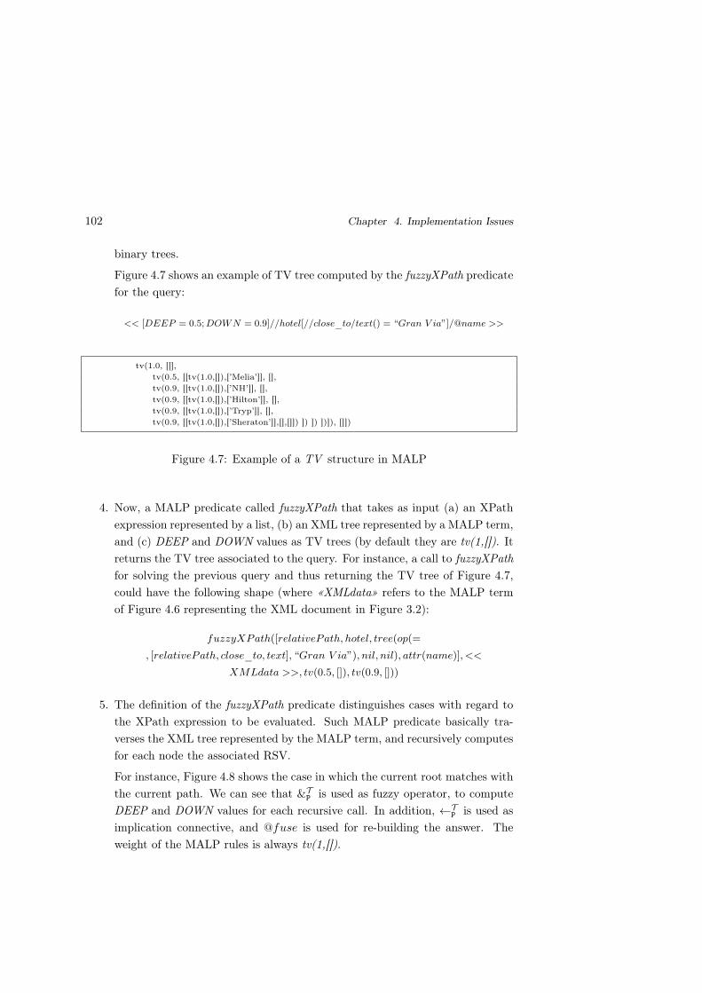
102 Chapter 4. Implementation Issues
binary trees.
Figure 4.7 shows an example of TV tree computed by the fuzzyXPath predicate
for the query:
<< [DEEP = 0.5;DOWN = 0.9]//hotel[//close_to/text() = “Gran V ia”]/@name >>
tv(1.0, [[],
tv(0.5, [[tv(1.0,[]),[’Melia’]], [],
tv(0.9, [[tv(1.0,[]),[’NH’]], [],
tv(0.9, [[tv(1.0,[]),[’Hilton’]], [],
tv(0.9, [[tv(1.0,[]),[’Tryp’]], [],
tv(0.9, [[tv(1.0,[]),[’Sheraton’]],[],[]]) ]) ]) ])]), []])
Figure 4.7: Example of a TV structure in MALP
4. Now, a MALP predicate called fuzzyXPath that takes as input (a) an XPath
expression represented by a list, (b) an XML tree represented by a MALP term,
and (c) DEEP and DOWN values as TV trees (by default they are tv(1,[]). It
returns the TV tree associated to the query. For instance, a call to fuzzyXPath
for solving the previous query and thus returning the TV tree of Figure 4.7,
could have the following shape (where «XMLdata» refers to the MALP term
of Figure 4.6 representing the XML document in Figure 3.2):
fuzzyXPath([relativePath, hotel, tree(op(=
, [relativePath, close_to, text], “Gran V ia”), nil, nil), attr(name)], <<
XMLdata >>, tv(0.5, []), tv(0.9, []))
5. The definition of the fuzzyXPath predicate distinguishes cases with regard to
the XPath expression to be evaluated. Such MALP predicate basically tra-
verses the XML tree represented by the MALP term, and recursively computes
for each node the associated RSV.
For instance, Figure 4.8 shows the case in which the current root matches with
the current path. We can see that &TP is used as fuzzy operator, to compute
DEEP and DOWN values for each recursive call. In addition, ←TP is used as
implication connective, and @fuse is used for re-building the answer. The
weight of the MALP rules is always tv(1,[]).
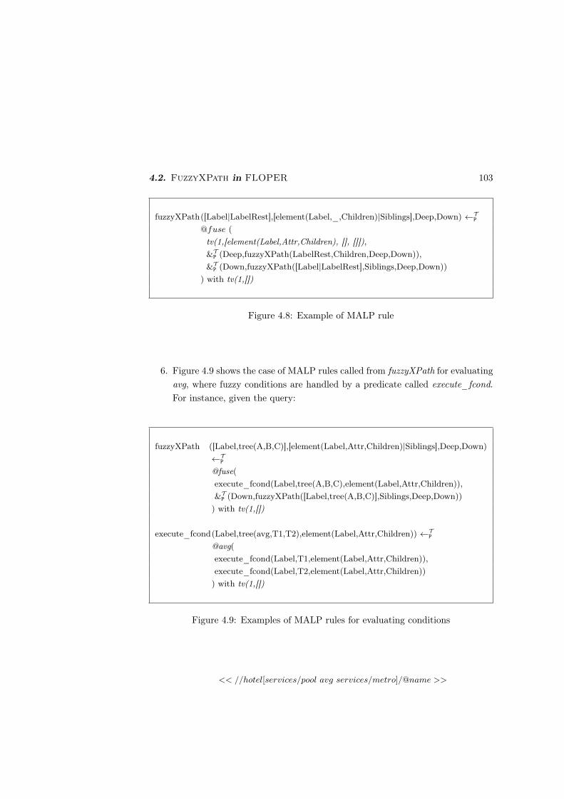
4.2. FuzzyXPath in FLOPER 103
fuzzyXPath([Label|LabelRest],[element(Label,_,Children)|Siblings],Deep,Down) ←TP
@fuse (
tv(1,[element(Label,Attr,Children), [], []]),
&TP (Deep,fuzzyXPath(LabelRest,Children,Deep,Down)),
&TP (Down,fuzzyXPath([Label|LabelRest],Siblings,Deep,Down))
) with tv(1,[])
Figure 4.8: Example of MALP rule
6. Figure 4.9 shows the case of MALP rules called from fuzzyXPath for evaluating
avg, where fuzzy conditions are handled by a predicate called execute_fcond.
For instance, given the query:
fuzzyXPath ([Label,tree(A,B,C)],[element(Label,Attr,Children)|Siblings],Deep,Down)
←TP
@fuse(
execute_fcond(Label,tree(A,B,C),element(Label,Attr,Children)),
&TP (Down,fuzzyXPath([Label,tree(A,B,C)],Siblings,Deep,Down))
) with tv(1,[])
execute_fcond(Label,tree(avg,T1,T2),element(Label,Attr,Children)) ←TP
@avg(
execute_fcond(Label,T1,element(Label,Attr,Children)),
execute_fcond(Label,T2,element(Label,Attr,Children))
) with tv(1,[])
Figure 4.9: Examples of MALP rules for evaluating conditions
<< //hotel[services/pool avg services/metro]/@name >>

104 Chapter 4. Implementation Issues
the corresponding call to the fuzzyXPath predicate would be:
fuzzyXPath([relativePath, hotel, tree(avg,
tree(exist([services, pool]), nil, nil),
tree(exist([services,metro]), nil, nil)),
attr(name)], << XMLdata >>, tv(1.0, []), tv(1.0, []))
which eventually will invoke predicate execute_fcond (for evaluating the fuzzy
condition containing the avg operator) as follows:
execute_fcond(hotel, tree(avg,
tree(exist([services, pool]), nil, nil),
tree(exist([services,metro]), nil, nil)),
<< XMLdata >>, TV _Cond)
Figure 4.10 shows the resulting TV tree, which clearly resembles the XML file
previously reported in Example 3.3.1.
tv(1.0,[[],
tv(1.0,[[tv(1.0, []), [Melia]], [],
tv(1.0,[[tv(1.0, []), [Tryp]], [],
tv(1.0,[[tv(1.0, []), [Sheraton]], [],
tv(1.0,[[tv(0.5, []), [NH]], [],
tv(1.0,[[tv(0.5, []), [Hilton]], [], []])])])])]), []])
Figure 4.10: Example of a TV obtained after evaluating a fuzzy condition
We have developed a prototype of our FuzzyXPath which is publicly available
from http://dectau.uclm.es/fuzzyXPath/, equipped with a Web interface from
which XPath queries can be tested. The implementation has been developed with
our FLOPER tool. In what follows, we will give some details about FLOPER and
the implementation of the FuzzyXPath in FLOPER.
Firstly, we would like to summarize the main elements of the FLOPER tool
[MM08, MMPV10a, MMPV11b] which manages MALP programs. The parser of our

4.2. FuzzyXPath in FLOPER 105
member(X):− number(X),0=<X,X=<1.
bot(0). top(1). leq(X,Y):− X=<Y.
or_prod(X,Y,Z):− pri_prod(X,Y,U1),pri_add(X,Y,U2),pri_sub(U2,U1,Z).
and_prod(X,Y,Z):− pri_prod(X,Y,Z).
pri_prod(X,Y,Z):− Z is X ∗ Y.
pri_add(X,Y,Z):− Z is X+Y.
pri_sub(X,Y,Z):− Z is X−Y.
Figure 4.11: Example of multi-adjoint lattice
FLOPER tool has been implemented by using the classical DCG’s (Definite Clause
Grammars) resource of the Prolog language, since it is a convenient notation for
expressing grammar rules. Once the application is loaded inside a Prolog interpreter,
it shows a menu which includes options for loading/compiling, parsing, listing and
saving fuzzy programs, as well as for executing/debugging fuzzy goals. All these
actions are based on the compilation of the fuzzy code into standard Prolog code.
The key point of the compilation is to extend each atom with an extra argument,
called truth variable of the form “_TVi”, which is intended to contain the truth degree
obtained after the subsequent evaluation of the atom. For instance, the first clause
of Figure 4.1 is translated into:
p(X,_TV0):−q(X,Y,_TV1),r(Y,_TV2),or_prod(_TV1,_TV2,_TV3),and_prod(0.8,_TV3,_TV0).
Moreover, the remaining rules, become the pure Prolog facts “q(a, Y, 0.9)” and
“r(b,0.7)”, whereas the corresponding lattice is expressed by the clauses of Figure
4.11, where the meaning of the mandatory predicates member, top, bot and leq is
obvious.
Finally, a fuzzy goal like “p(X)”, is translated into the pure Prolog goal:
p(X,Truth_degree)
(note that the last truth degree variable is not anonymous now) for which, after
choosing option “run”, the Prolog interpreter returns the desired fuzzy computed
answer:
[Truth_degree = 0.776, X = a]
Note that all internal computations (including compiling and executing) are pure
Prolog derivations, whereas inputs (fuzzy programs and goals) and outputs (fuzzy
computed answers) have always a fuzzy taste, thus producing the illusion on the

106 Chapter 4. Implementation Issues
final user of being working with a purely fuzzy logic programming tool. By using
option “ lat” (“show”) of FLOPER, we can associate (and visualize) a new lattice to
a given program. As seen before, such lattices must be expressed by means of a set
of Prolog clauses (defining predicates member, top, bot, leq and the ones associated
to fuzzy connectives) in order to be loaded into FLOPER.
Although the core of our implementation is written with (fuzzy) MALP rules,
we have reused/adapted several modules of our previous Prolog-based implementa-
tion of (crisp) XPath described in [ABE08, Alm09], which make use of the SWI-
Prolog library for loading XML files in order to store each XML document by means
of a Prolog term. For loading XML documents in our implementation we use the
predicate load_xml(+File,-Term), and similarly, we have a predicate
write_xml(+File,+Term) for writing a data-term representing an XML document
into a file. And, of course, the parser of our application has been extended to
recognize the new keywords DEEP, DOWN, avg, etc... with the proper arguments.
Furthermore, we have incorporated a lattice definition according to the definitions
of Section 4.1.2, which is shown in Figure 4.12, where and, or and avg operators are
defined by Prolog rules. Figure 4.13 shows the Prolog compilation from FLOPER
of the rule of Figure 4.8. Finally, we have defined a predicate tv_to_elem to show
the result in a pretty way which transforms the returned TV tree to an XML tree.
4.3 XQuery Library FuzzyXPath
The implementation of our fuzzy extension of XPath is based on an XQuery library
too, the functions including deep and down operators, as well as the fuzzy operators
and+, and-, and, or+, or-, or and avg. Using this library the user can replace
Boolean operators by fuzzy versions in XPath expressions, as well as he (she) can
call to deep and down operators, in order to obtain ranked sets of answers. The
answers are shown with a Retrieval State Value (RSV) representing the degree of
satisfaction. The answers can also be ordered with respect to the RSV making use
of descending XQuery expression, as well as filtered with regard to a threshold.
The implementation of our fuzzy extension of XPath is based on an XQuery
library of functions including deep and down operators, as well as the fuzzy operators
and+, and-, and, or+, or-, or and avg. Using this library the user can replace
Boolean operators by fuzzy versions in XPath expressions, as well as he (she) can
call to deep and down operators, in order to obtain ranked sets of answers. The

4.3. XQuery Library FuzzyXPath 107
and_prod(tv(X1,X2),tv(Y1,Y2),tv(Z1,Z2)):−
pri_prod(X1,Y1,Z1),pri_app(X2,Y2,Z2).
and_luka(tv(X,Elem1),tv(Y,Elem2),tv(Z,Elem0)):−
pri_add(X,Y,U1), pri_sub(U1,1,U2),
pri_max(U2,0.0,Z), pri_app(Elem1, Elem2, Elem0).
and_godel(tv(X,Elem1),tv(Y,Elem2),tv(Z,Elem0)):−
pri_min(X,Y,Z), pri_app(Elem1,Elem2,Elem0).
or_prod(tv(X1,X2),tv(Y1,Y2),tv(Z1,Z2)):− pri_prod(X1,Y1,U1),
pri_add(X1,Y1,U2),pri_sub(U2,U1,Z1),
pri_app(X2,Y2,Z2).
or_luka(tv(X,Elem1),tv(Y,Elem2),tv(Z,Elem0)):−
pri_add(X,Y,U1), pri_min(U1,1,Z),
pri_app(Elem1,Elem2,Elem0).
or_godel(tv(X,Elem1),tv(Y,Elem2),tv(Z,Elem0)):−
pri_max(X,Y,Z), pri_app(Elem1,Elem2,Elem0).
agr_aver(tv(X1,X2),tv(Y1,Y2),tv(Z1,Z2)):− pri_add(X1,Y1,Aux),
pri_div(Aux,2,Z1),pri_app(X2,Y2,Z2).
agr_avg(tv(V1,E1),tv(V2,E2),tv(T1,F1),tv(T2,F2),tv(V3,G)):−
V3 is (V1∗T1 + V2∗T2)/(T1+T2),pri_app(E1,E2,A1),
pri_app(F1,F2,A2),pri_app(A1,A2,G).
pri_add(X,Y,Z) :− Z is X+Y. pri_sub(X,Y,Z) :−Z is X−Y.
pri_prod(X,Y,Z) :− Z is X ∗ Y. pri_div(X,Y,Z) :− Z is X/Y.
pri_app([],[],[]):−!.
pri_app([],A,A):−!.
pri_app(A,[],A):−!.
pri_app([Element,TV_Son,[]],TV_SibA,[Element,TV_Son,TV_SibA]):−!.
pri_app([Element,TV_Son,TV_sib],TV_SibA,[Element,TV_Son,TV_SibR]):−
pri_app(TV_sib,TV_SibA,[Element,TV_Son,TV_SibR]),!.
Figure 4.12: Multi-adjoint lattice for FuzzyXPath (file “tv.pl”)
answers are shown with a Retrieval State Value (RSV) representing the degree of
satisfaction. The answers can also be ordered with respect to the RSV making use
of descending XQuery expression, as well as filtered with regard to a threshold.
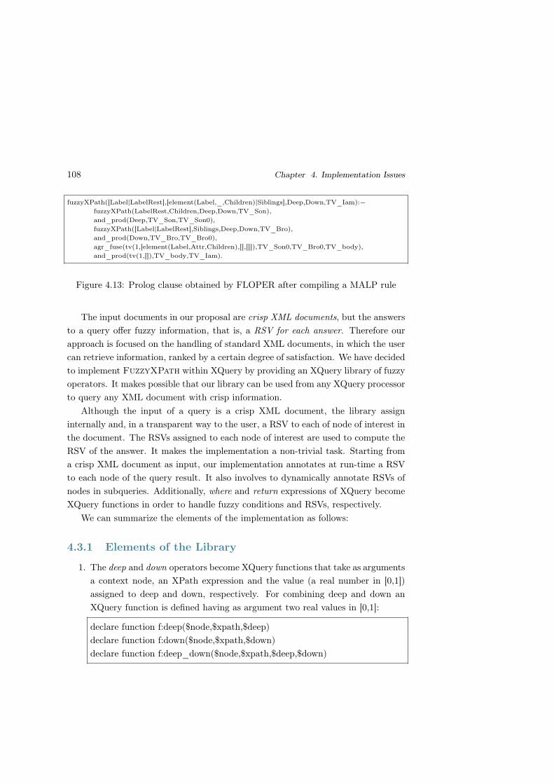
108 Chapter 4. Implementation Issues
fuzzyXPath([Label|LabelRest],[element(Label,_,Children)|Siblings],Deep,Down,TV_Iam):−
fuzzyXPath(LabelRest,Children,Deep,Down,TV_Son),
and_prod(Deep,TV_Son,TV_Son0),
fuzzyXPath([Label|LabelRest],Siblings,Deep,Down,TV_Bro),
and_prod(Down,TV_Bro,TV_Bro0),
agr_fuse(tv(1,[element(Label,Attr,Children),[],[]]),TV_Son0,TV_Bro0,TV_body),
and_prod(tv(1,[]),TV_body,TV_Iam).
Figure 4.13: Prolog clause obtained by FLOPER after compiling a MALP rule
The input documents in our proposal are crisp XML documents, but the answers
to a query offer fuzzy information, that is, a RSV for each answer. Therefore our
approach is focused on the handling of standard XML documents, in which the user
can retrieve information, ranked by a certain degree of satisfaction. We have decided
to implement FuzzyXPath within XQuery by providing an XQuery library of fuzzy
operators. It makes possible that our library can be used from any XQuery processor
to query any XML document with crisp information.
Although the input of a query is a crisp XML document, the library assign
internally and, in a transparent way to the user, a RSV to each of node of interest in
the document. The RSVs assigned to each node of interest are used to compute the
RSV of the answer. It makes the implementation a non-trivial task. Starting from
a crisp XML document as input, our implementation annotates at run-time a RSV
to each node of the query result. It also involves to dynamically annotate RSVs of
nodes in subqueries. Additionally, where and return expressions of XQuery become
XQuery functions in order to handle fuzzy conditions and RSVs, respectively.
We can summarize the elements of the implementation as follows:
4.3.1 Elements of the Library
1. The deep and down operators become XQuery functions that take as arguments
a context node, an XPath expression and the value (a real number in [0,1])
assigned to deep and down, respectively. For combining deep and down an
XQuery function is defined having as argument two real values in [0,1]:
declare function f:deep($node,$xpath,$deep)
declare function f:down($node,$xpath,$down)
declare function f:deep_down($node,$xpath,$deep,$down)

4.3. XQuery Library FuzzyXPath 109
2. Fuzzy versions of Boolean operators and, or have been defined as XQuery func-
tions, each one for each fuzzy logic we have considered (i.e., Product, Łukasie-
wicz and Gödel):
declare function f:andP($left,$right)
declare function f:orP($left,$right)
declare function f:andG($left,$right)
declare function f:orG($left,$right)
declare function f:andL($left,$right)
declare function f:orL($left,$right)
3. Operators avg and avga,b have been defined as XQuery functions:
declare function f:avg($left,$right)
declare function f:avg_ab($left,$right,$a,$b)
4. Fuzzy versions of XQuery expressions where and return have been defined.
In order to make transparent to the user the incorporation of RSVs, we have
defined a new version of the return expression, called returnF, which trans-
parently carries out the computation of the RSVs of the answers. Similarly,
since XQuery works with a Boolean logic, the introduction of fuzzy versions of
the operators, force us to define a new version of the where expression, called
whereF, which transparently carries out the computation of the RSVs from
fuzzy conditions. ReturnF has as parameters the context node and an XPath
expression. WhereF has as parameters the context node and a fuzzy condition.
declare function f:whereF($node,$fuzzycond)
declare function f:returnF($node,$xpath)
5. Fuzzy versions of comparison operators for XPath expressions have been de-
fined as XQuery functions. Similarly to whereF, comparison operators have
been adapted to handle the RSVs:
declare function f:equalF($left,$right)
declare function f:lessF($left,$right)
declare function f:greaterF($left,$right)
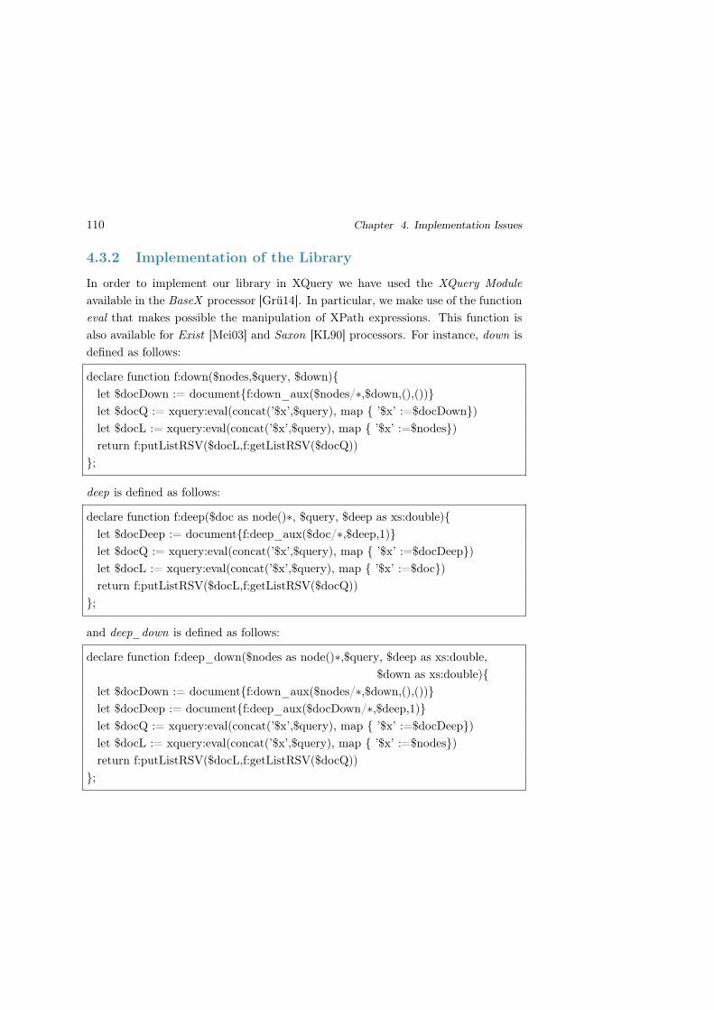
110 Chapter 4. Implementation Issues
4.3.2 Implementation of the Library
In order to implement our library in XQuery we have used the XQuery Module
available in the BaseX processor [Grü14]. In particular, we make use of the function
eval that makes possible the manipulation of XPath expressions. This function is
also available for Exist [Mei03] and Saxon [KL90] processors. For instance, down is
defined as follows:
declare function f:down($nodes,$query, $down)
let $docDown := documentf:down_aux($nodes/∗,$down,(),())
let $docQ := xquery:eval(concat(’$x’,$query), map ’$x’ :=$docDown)
let $docL := xquery:eval(concat(’$x’,$query), map ’$x’ :=$nodes)
return f:putListRSV($docL,f:getListRSV($docQ))
;
deep is defined as follows:
declare function f:deep($doc as node()∗, $query, $deep as xs:double)
let $docDeep := documentf:deep_aux($doc/∗,$deep,1)
let $docQ := xquery:eval(concat(’$x’,$query), map ’$x’ :=$docDeep)
let $docL := xquery:eval(concat(’$x’,$query), map ’$x’ :=$doc)
return f:putListRSV($docL,f:getListRSV($docQ))
;
and deep_down is defined as follows:
declare function f:deep_down($nodes as node()∗,$query, $deep as xs:double,
$down as xs:double)
let $docDown := documentf:down_aux($nodes/∗,$down,(),())
let $docDeep := documentf:deep_aux($docDown/∗,$deep,1)
let $docQ := xquery:eval(concat(’$x’,$query), map ’$x’ :=$docDeep)
let $docL := xquery:eval(concat(’$x’,$query), map ’$x’ :=$nodes)
return f:putListRSV($docL,f:getListRSV($docQ))
;

4.3. XQuery Library FuzzyXPath 111
Each fuzzy operator has been defined as a function, for instance, and (Product
logic), or+ (Gödel logic), avg, and avga,b are defined as follows:
declare function f:andP($cond1,$cond2)
let $tv1 := f:truthValue($cond1)
let $tv2 := f:truthValue($cond2)
return $tv1∗$tv2
;
declare function f:orG($cond1,$cond2)
let $tv1 := f:truthValue($cond1)
let $tv2 := f:truthValue($cond2)
return
if ($tv1 > $tv2) then $tv1
else $tv2
;
declare function f:avg($cond1,$cond2)
let $tv1 := f:truthValue($cond1)
let $tv2 := f:truthValue($cond2)
return (xs:double($tv1)+xs:double($tv2)) div (2)
;
declare function f:avg_ab($cond1,$cond2, $a, $b)
let $tv1 := f:truthValue($cond1)
let $tv2 := f:truthValue($cond2)
return (xs:double($tv1)∗$a+xs:double($tv2)∗$b) div ($a+$b)
;
4.3.3 Examples of FuzzyXPath in XQuery
Now, we show how the previous FuzzyXPath queries can be written in XQuery.
Let us now suppose the following FuzzyXPath query:

112 Chapter 4. Implementation Issues
<< /hotels/hotel[[DOWN = 0.9]close_to/text() = “Sol”]/@name >>
We can now write the same query in XQuery as follows:
for $x in doc(’hotels.xml’)/hotels/hotel
let $y := f:whereF($x,f:equalF(f:down($x,’/close_to’,0.9),’Sol’))
let $z := f:returnF($y,’/@name’)
order by $y/@rsv descending
return $z
We can see that FuzzyXPath expressions are written as XQuery expressions. This
is the same kind of transformation from crisp XPath to XQuery. For instance:
<< /hotels/hotel[close_to/text() = “Sol”]/@name >
can be translated into:
for $x in doc("hotels.xml")/hotels/hotel
where $x/close_to/text()="Sol"
return $x/@name
In the fuzzy case, “=” is transformed into equalF, and where as well as return
become XQuery functions, with an extra argument to represent the context node.
The query makes use of the function down of the library to compute the RSVs
associated to close_to. In addition, the attribute rsv, which has been (internally)
added to the output document, can be handled to show the answer in a sorted way,
and even to define a threshold.
Let us now consider the following query, that uses deep and down:
<< /hotels/hotel[[DEEP = 0.5;DOWN = 0.9]//close_to/text() = “Callao”]/@name >>
We can now write the same query in XQuery using the function deep_down:
for $x in doc(’hotels.xml’)/hotels/hotel
let $y :=
f:whereF($x, f:equalF(f:deep_down($x,’//close_to’,0.5,0.9),’Callao’))
let $z := f:returnF($y,’/@name’)
order by $y/@rsv descending
return $z

4.3. XQuery Library FuzzyXPath 113
Let us now suppose the following FuzzyXPath expression that makes use of the
avg operator.
<< //hotel[services/pool avg services/metro]/@name >>
Here, we use the function avg of the library, having as parameters both sides of the
fuzzy condition:
for $x in doc(’hotels.xml’)//hotel
let $y := f:whereF($x, f:avg($x/services/pool,$x/services/metro))
let $z := f:returnF($y,’/@name’)
order by $y/@rsv descending
return $z
The same can be said for the following query, using avga,b having as parameters
a and b.
<< //hotel[services/pool avg1, 2 services/metro]/@name >>
for $x in doc(’hotels.xml’)//hotel
let $y := f:whereF($x,f:avg_ab($x/services/pool, $x/services/metro,1,2))
let $z := f:returnF($y,’/@name’)
order by $y/@rsv descending
return $z
Let us now suppose the following queries that combine deep and avg, and deep
and and+, respectively:
<< //hotel[[DEEP = 0.8]//close_to/text() = “Sol”avg1, 2 //price/text() < 150]/@name >>
for $x in doc(’hotels.xml’)//hotel
let $y := f:whereF($x, f:avg_ab(f:equalF(f:deep($x,’//close_to’,0.8),’Sol’),
$x//price/text()<150,1,2))
let $z := f:returnF($y,’/@name’)
order by $y/@rsv descending
return $z

114 Chapter 4. Implementation Issues
<< //hotel[([DEEP = 0.5]//close_to/text() = ”GranV ia”) and+ (//pool avg3, 2 //metro/text() < 200)]/@name >>
for $x in doc(’hotels.xml’)//hotel
let $y := f:whereF($x,f:andG(f:equalF(f:deep($x,’//close_to’,0.5),’GranVia’),
f:avg_ab($x//pool,$x//metro<200,3,2)))
let $z := f:returnF($y,’/@name’)
order by $y/@rsv descending
return $z
4.3.4 Benchmarks
Now, we would like to show the benchmarks we have obtained using our library. We
have tested our library using data sets of different sizes. We have used as data sets
traces of execution of MALP programs developed under our FLOPER tool. The
FLOPER tool generates traces in XML format, with a high degree of tag nesting
when a recursive program is executed. These data sets facilitate the testing of our
structural based operators deep and down.
Query 16Kb 700Kb 4.8Mb 15.4Mb
Examined nodes in Q1 28 148 298 448
Examined nodes in Q2 25 145 295 445
Tree Depth 21 101 201 301
Q1 7.09 ms 25.47 ms 123.66 ms 461.6 ms
down in Q1 12.52 ms 107.1 ms 481.24 ms 2853.36 ms
deep in Q1 10.08 ms 74.17 ms 510.74 ms 1953.31 ms
deep and down in Q1 69.97 ms 102.0 ms 685.87 ms 7315.59 ms
Q2 5.77 ms 57.96 ms 172.03 ms 529.18 ms
avg in Q2 36.59 ms 1266.99 ms 9729.49 ms 60426.28 ms
Figure 4.14: Benchmarks
In Figure 4.14 we can see the results, where we indicate the number of nodes
examined in each tree, as well as the depth of the tree. We have compared the
execution times for two XPath expressions in crisp and fuzzy versions.

4.3. XQuery Library FuzzyXPath 115
The first query is Q1:
<< //node/goal >>
and the second query is Q2:
<< //node[goal[contains(text(), ”p(”)] and substitution[contains(text(), ”g(”)]]//goal >>
We have used the BaseX Query processor in a Intel Core 2 Duo 2.66 GHz Mac
OS machine.

116 Chapter 4. Implementation Issues

Chapter 5
The FuzzyXPath debugger
The XPath language [BBC+07] was designed as a query language for XML in which
the path of the tree is used to describe the query. In spite of the simplicity of the
XPath language, the programmer usually makes mistakes when (s)he describes the
path in which the data are allocated. Tipically, (s)he omits some of the tags of the
path, s(he) adds more than necessary, and (s)he also uses similar but wrong tag
names. When the query does not match to the tree structure of the XML tree, the
answer is empty. However, we can also find the case in which the query matches to
the XML tree but the answer does not satisfy the programmer. Due to the inherent
flexibility of XML documents, the same tag can occur at several positions, and the
programmer could find answers that do not correspond to her(is) expectations. In
other words, (s)he finds a correct path, but a wrong answer. We can also consider the
case in which a boolean condition is wrong, expressing a wrong range, and several
conditions that do not hold at the same time. When the programmer does not find
the answer (s)he is looking for, there is a mechanism that (s)he can try to debug
the query. In XPath there exists an operator, denoted by ‘//’, that permits to look
for the tag from that position. However, it is useless when the tag is present at
several positions, since even though the programmer finds answers, (s)he does not
know whether they are close to h(er) expectations.
XPath debugging has to take into account the previous considerations. Par-
ticularly, there is an underlying notion of chance degree. When the programmer
makes mistakes, the number of bugs can be higher or lower, and the chance degree
is proportional to them. Moreover, there are several ways on which each bug can
117

118 Chapter 5. The FuzzyXPath debugger
be solved, and therefore the chance degree is also dependent from the number of
solutions for each bug, and the quality of each solution. The quality of a solution
describes the number of changes to be made. Finally, there is a case in which we
have also focused our work. The case in which the mistake comes from a similar but
wrong tag. Here, the chance degree represents the semantic similarity between the
tag expressed in the query and the tag which really appears in the XML document.
We will describe how we can manipulate an XPath expression in order to obtain
a set of alternative XPath expressions that match to a given XML document. For
each alternative XPath expression we will give a chance degree that represents the
degree in which the expression deviates from the initial expression. Thus, our work
is focused on providing the programmer a repertoire of paths that (s)he can use to
retrieve answers.
We propose that XPath debugging is guided by the programmer that initially
establishes a value (a real value between 0 and 1), that the debugger uses to penalize
each bug. Each bug found is penalized with such a value, and thus the chance degree
is proportional to the value. Additionally, we assume that the debugger is equipped
with a table of similarities, that is, a table in which pairs of similar words are
assigned to a value between 0 and 1. It makes possible that chance degree is also
computed from similarity degrees. The debugger reports a set of annotated paths in
an extended XPath syntax in which we have incorporated three annotations: JUMP,
SWAP and DELETE. JUMP is used to represent that some tags have been added
to the original expression, SWAP is used to represent that a tag has been changed
by another, and DELETE is used to represent that a tag has been removed. The
reported XPath expressions update the original XPath expression, that is, the case
JUMP incorporates ‘//’ at the position in which the bug is found, the case SWAP
includes the new tag, and the case DELETE removes the wrong tag.
Additionally, our proposal permits the programmer tests the reported XPath ex-
pressions. The annotated XPath expressions can be executed obtaining a ranked set
of answers with respect to the chance degree. It facilitates the process of debugging
because the programmer can visualize the answers to each query.
The approach has been implemented and tested (see http://dectau.uclm.es/
fuzzyXPath/?q=DebuggerXPathTest). Additionally, our proposal permits the pro-
grammer to test the reported XPath expressions. The annotated XPath expressions
can be executed in our tool (http://dectau.uclm.es/fuzzyXPath/) in order to
obtain a ranked set of answers w.r.t. the chance degree. It facilitates the pro-

5.1. Debugging XPath 119
cess of debugging because programmers can visualize answers to each query in a
very easy way. Our implementation has been developed on top of the recently
proposed FuzzyXPath extension [ALM11a, ALM12c], which uses fuzzy logic pro-
gramming to provide a fuzzy taste to XPath expressions. The implementation has
been coded with the fuzzy logic programming language MALP and developed
with the FLOPER tool designed in our research group and freely accessible from
http://dectau.uclm.es/floper/.
Although our approach can be applied to standard (crisp) XPath expressions,
chance degrees in XPath debugging fits well with our proposal. Particularly, XPath
debugging annotations can be seen as annotations of XPath expressions similary
to the proposed DEEP and DOWN of FuzzyXPath [ALM11a, ALM12c]. DEEP
and DOWN serve to annotate XPath expressions and to obtain a ranked set of
answers depending on they occur, more deeply and from top to down. Each answer
is annotated with a RSV (Retrieval Status Value) which describes the degree of
satisfaction of the answer. Here JUMP, SWAP and DELETE penalize the answers
of annotated XPath expressions. DEEP and JUMP have, in fact, the same behavior:
JUMP proportionally penalizes answers as deep as they occur. Moreover, in order
to cover with SWAP, we have incorporated to our framework similarity degrees.
5.1 Debugging XPath
In this section we propose a debugging technique for XPath expressions. Our debug-
ging process accepts as inputs a query Q preceded by the [DEBUG = r] command,
where r is a real number in the unit interval. For instance,
<< [DEBUG = 0.5]/bib/book/title >>
Assuming an input XML document like the one depicted in Figures 5.2 and 5.1,
the debugging produces a set of alternative queries Q1, ..., Qn packed into an output
XML document, like the one shown in Figure 5.3. The document has the following
structure:

120 Chapter 5. The FuzzyXPath debugger
<bib>
<name>Classic Literature</name>
<book year="2001" price="45.95">
<title>Don Quijote de la Mancha</title>
<author>Miguel de Cervantes Saavedra</author>
<references>
<novel year="1997" price="35.99">
<name>La Galatea</name>
<author>Miguel de Cervantes Saavedra</author>
<references>
<book year="1994" price="25.99">
<title>Los trabajos de Persiles y Sigismunda</title>
<author>Miguel de Cervantes Saavedra</author>
</book>
</references>
</novel>
</references>
</book>
<novel year="1999" price="25.65">
<title>La Celestina</title>
<author>Fernando de Rojas</author>
</novel>
</bib>
Figure 5.1: Input XML document in our examples with Debug
BookTitle
Author
Name
Name
References
AuthorNovel
BIB
Title
References
AuthorBook
NovelTitle
Author
Figure 5.2: XML skeleton represented as a tree
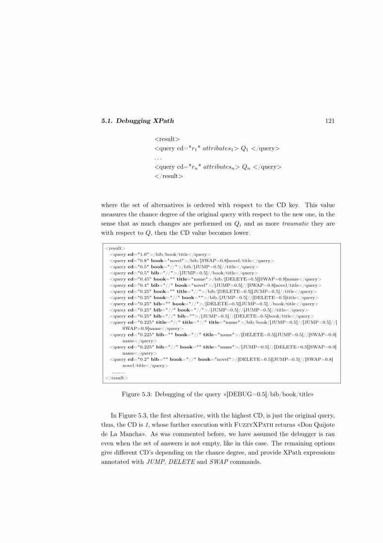
5.1. Debugging XPath 121
<result>
<query cd="r1" attributes1> Q1 </query>
. . .
<query cd="rn" attributesn> Qn </query>
</result>
where the set of alternatives is ordered with respect to the CD key. This value
measures the chance degree of the original query with respect to the new one, in the
sense that as much changes are performed on Qi and as more traumatic they are
with respect to Q, then the CD value becomes lower.
<result>
<query cd="1.0">/bib/book/title</query>
<query cd="0.8" book="novel">/bib/[SWAP=0.8]novel/title</query>
<query cd="0.5" book="//">/bib/[JUMP=0.5]//title</query>
<query cd="0.5" bib="//">/[JUMP=0.5]//book/title</query>
<query cd="0.45" book="" title="name">/bib/[DELETE=0.5][SWAP=0.9]name</query>
<query cd="0.4" bib="//" book="novel">/[JUMP=0.5]//[SWAP=0.8]novel/title</query>
<query cd="0.25" book="" title="//">/bib/[DELETE=0.5][JUMP=0.5]//title</query>
<query cd="0.25" book="//" book="">/bib/[JUMP=0.5]//[DELETE=0.5]title</query>
<query cd="0.25" bib="" book="//">/[DELETE=0.5][JUMP=0.5]//book/title</query>
<query cd="0.25" bib="//" book="//">/[JUMP=0.5]//[JUMP=0.5]//title</query>
<query cd="0.25" bib="//" bib="">/[JUMP=0.5]//[DELETE=0.5]book/title</query>
<query cd="0.225" title="//" title="//" title="name">/bib/book/[JUMP=0.5]//[JUMP=0.5]//[
SWAP=0.9]name</query>
<query cd="0.225" bib="" book="//" title="name">/[DELETE=0.5][JUMP=0.5]//[SWAP=0.9]
name</query>
<query cd="0.225" bib="//" book="" title="name">/[JUMP=0.5]//[DELETE=0.5][SWAP=0.9]
name</query>
<query cd="0.2" bib="" book="//" book="novel">/[DELETE=0.5][JUMP=0.5]//[SWAP=0.8]
novel/title</query>
.........
</result>
Figure 5.3: Debugging of the query «[DEBUG=0.5]/bib/book/title»
In Figure 5.3, the first alternative, with the highest CD, is just the original query,
thus, the CD is 1, whose further execution with FuzzyXPath returns «Don Quijote
de La Mancha». As was commented before, we have assumed the debugger is ran
even when the set of answers is not empty, like in this case. The remaining options
give different CD’s depending on the chance degree, and provide XPath expressions
annotated with JUMP, DELETE and SWAP commands.

122 Chapter 5. The FuzzyXPath debugger
In order to explain the way in which our technique generates the attributes and
content of each query tag in the output XML document, let us consider a generic
path Q of the form:
<< [DEBUG = r]/tag1/.../tagi/tagi+1/... >>
where we say that tagi is at level i in the original query. So, assume that during the
exploration of the input query Q and the XML document D, we find that tagi in Q
does not occurs at level i in (a branch of) D. Then, we consider the following three
situations:
Swapping case: Instead of tagi, we find tag′i at level i in the input XML document
D, being tagi and tag′i two similar terms with similarity degree s. Then, we generate
an alternative query by adding the attribute tagi ="tag′i" and replacing in the
original path the occurrence "tagi/" by "[SWAP = s]tag′i/".
The second query proposed in Figure 5.3 illustrates this case:
< query cd = “0.8” book = “novel” > /bib/[SWAP = 0.8]novel/title < /query >
Let us observe that : 1) we have included the attribute «book=“novel"» in order
to suggest that instead of looking now for a book, finding a novel should be also a
good alternative, 2) in the path we have replaced the tag book by novel and we have
appropriately annotated the exact place where the change has been performed with
the annotation [SWAP = 0.8] and 3) the CD of the new query has been adjusted
with the similarity degree 0.8 of the exchanged tags.
Now, we can run the (fuzzy) XPath queries «/bib/novel/title» and even
«/bib/[SWAP = 0.8]novel/title» (see Figure 5.4). In both cases we obtain the
same result, i.e., «La Celestina», but with different RSV (or Retrieval Status Value):
1 and 0.8, respectively.
<result>
<title rsv="0.8">La Celestina</title>
</result>
Figure 5.4: Execution of the query «/bib/[SWAP = 0.8]novel/title»

5.1. Debugging XPath 123
Jumping case: Even when tagi is not found at level i in the input XML document
D, tagi+1 appears at a deeper level (i.e., greater than i) in a branch of D. Then,
we generate an alternative query by adding the attribute tagi="//", which means
that tagi has been jumped, and replacing in the path the occurrence "tag_i/" by
"[JUMP = r]//", being r the value associated to DEBUG.
<result>
<title rsv="0.5">Don Quijote de la Mancha</title>
<title rsv="0.5">La Celestina</title>
<title rsv="0.03125">Los trabajos de Persiles y Sigismunda</title>
</result>
Figure 5.5: Execution of the query «/bib/[JUMP = 0.5]//title»
<result>
<title rsv="0.5">Don Quijote de la Mancha</title>
<title rsv="0.03125">Los trabajos de Persiles y Sigismunda</title>
</result>
Figure 5.6: Execution of the query «/[JUMP = 0.5]//book/title»
This situation is illustrated by the third and fourth queries in Figure 5.3, where
we propose to jump the tags book and bib. The execution of the queries returns
different results, as shown in Figures 5.5 and 5.6, where JUMP produces similar
effects to the DEEP command explained in the previous section, that is, as more tags
are jumped their resulting CD’s become lower.
Deletion case: This situation emerges when at level i in the input XML document
D, we found tagi+1 instead of tagi. So, the intuition tell us that tagi should be
removed from the original query Q and hence, we generate an alternative query by
adding the attribute tagi="" and replacing in the path the occurrence "tag_i" by
"[DELETE = r]", being r the value associated to DEBUG.
This situation is illustrated by the fifth query in Figure 5.3, where the deletion
of the tag book is followed by a swapping of similar tags title and name. The CD
0.45 associated to this query is defined as the product of the values associated to
both DELETE (0.5) and SWAP (0.9), and hence the chance degree of the original
one is lower than the previous examples.

124 Chapter 5. The FuzzyXPath debugger
As seen in Figure 5.7, the execution of our new query is able to retrieve the
information contained in the first branch of the input XML document listed in
Figures 5.2 and 5.1. Here we illustrate that execution of debugged XPath expressions
reveals hidden answers that can fulfill the programmer expectations.
<result>
<name rsv="0.45">Classic Literature</name>
</result>
Figure 5.7: Execution of the query «/bib/[DELETE = 0.5][SWAP = 0.9]name»
As we have seen in the previous example, the combined use of one or more
debugging commands (SWAP, JUMP and DELETE) is not only allowed but also
frequent. In other words, it is possible to find several debugging points. In Figure
5.8, we can see the execution of the query:
< query cd = “0.225” bib = “” book = “//” title = “name” >
/[DELETE = 0.5][JUMP = 0.5]//[SWAP = 0.9]name < /query >
The CD 0.225 is quite low, and therefore the chance degree is low, since it has
been obtained by multiplying the three values associated to the deletion of the tag
bib (0.5), jumping the tag book (0.5) and the swapping of title by name (0.9).
<result>
<name rsv="0.225">Classic Literature</name>
<name rsv="0.028125">La Galatea</name>
</result>
Figure 5.8: Execution of the query «/[DELETE = 0.5][JUMP = 0.5]//[SWAP = 0.9]name»
The wide range of alternatives (Figure 5.3 is still incomplete), reveals the flex-
ibility of our technique. The programmer is free to use the alternative queries to
execute them, and to inspect results up to the expectations are covered.
Finally, we would like to remark that even when we have worked with a very sim-
ple query with three tags in our examples, our technique works with more complex
queries with large paths and connectives in boolean conditions, as well as DEBUG
used in several places on the query.

5.2. MALP and the XPath Debugger 125
For instance, in Figure 5.9 (compare it with Figure 5.3) we show the result of
debugging the following query:
«[DEBUG = 0.7]/bib/[DEBUG = 0.6]book/[DEBUG = 0.5]title»
<result>
<query cd="1.0">/bib/book/title</query>
<query cd="0.8" book="novel">/bib/[SWAP=0.8]novel/title</query>
<query cd="0.7" bib="//">/[JUMP=0.7]//book/title</query>
<query cd="0.6" book="//">/bib/[JUMP=0.6]//title</query>
<query cd="0.56" bib="//" book="novel">/[JUMP=0.7]//[SWAP=0.8]novel/title</query>
<query cd="0.54" book="" title="name">/bib/[DELETE=0.6][SWAP=0.9]name</query>
<query cd="0.42" bib="" book="//">/[DELETE=0.7][JUMP=0.6]//book/title</query>
<query cd="0.42" bib="//" book="//">/[JUMP=0.7]//[JUMP=0.6]//title</query>
<query cd="0.378" bib="" book="//" title="name">
/[DELETE=0.7][JUMP=0.6]//[SWAP=0.9]name</query>
<query cd="0.378" bib="//" book="" title="name">
/[JUMP=0.7]//[DELETE=0.6][SWAP=0.9]name</query>
<query cd="0.336" bib="" book="//" book="novel">
/[DELETE=0.7][JUMP=0.6]//[SWAP=0.8]novel/title</query>
<query cd="0.3" book="" title="//">/bib/[DELETE=0.6][JUMP=0.5]//title</query>
<query cd="0.2646" bib="//" bib="" book="" title="name">
/[JUMP=0.7]//[DELETE=0.7][DELETE=0.6][SWAP=0.9]name</query>
.........
</result>
Figure 5.9: Debugging of the query «[DEBUG = 0.7]/bib/[DEBUG = 0.6]book/[DEBUG = 0.5]title»
5.2 MALP and the XPath Debugger
The core of our debugger is coded with MALP rules by reusing most modules of
our FuzzyXPath interpreter [ALM11a, ALM11b]. And, of course, the parser of
our debugger has been extended to recognize the new keywords DEBUG, SWAP,
DELETE and JUMP, with their proper arguments.
Now, we would like to show how the new “XPath debugging” predicate admits
an elegant definition by means of fuzzy MALP rules. Each rule defining predicate:
debugQuery(ListXPath, Tree, Penalty)
receives three arguments: (1) ListXPath is the Prolog representation of an XPath
expression, (2) Tree is the term representing an input XML document and (3)

126 Chapter 5. The FuzzyXPath debugger
Penalty represents the chance degree. A call to this predicate returns a truth-value
(i.e., a tv tree) like the following one:
tv(1.0,[[/,[]],
tv(1.0, [[tag(bib),[]],
tv(1.0,[[tag(book),[]],
tv(1.0,[[tag(title),[]],[],
...
tv(0.8,[[tag(novel),[book=novel]],
...
tv(0.5,[[’[DELETE=0.5]’,[book=’’]],
tv(0.9,[[tag(name),[title=name]],[],
...
[]])]),
[]])]),
[]])])])]),
[]])
Basically, the debugQuery predicate traverses the XML document, checking the
validity of the original query tag-by-tag, and trying to match each tag to the ones
occurring in the XML document and thus producing effects of DELETE, JUMP and
SWAP.
The definition of such predicate includes several rules for distinguishing the three
debugging cases. As an example the case of swapping is defined as follows:
debugQuery([Label|LabelRest],[element(Label2,_,Children)|Siblings],Penalty) <prod
@fuse(
similarity(Label, Label2),
debugQuery(LabelRest, Children, Penalty),
debugQuery([Label|LabelRest], Siblings, Penalty)
) with tv(1,[]).
which becomes into the following Prolog clause after compilation into FLOPER:
debugQuery([Label|LabelRest],[element(Label2,_,Children)|Siblings], Penalty, TV_Iam):−
similarity(Label, Label2, TV_Similarity),
debugQuery(LabelRest, Children, Penalty, TV_Son),
debugQuery([Label|LabelRest], Siblings, Penalty, TV_Sib),
agr_fuse(TV_Similarity, TV_Son, TV_Sib, TV_Iam).
Basically, similarity is checked with the atom similarity(Label, Label2), and two re-
cursive calls are achieved for debugging both children (debugQuery(LabelRest, Chil-
dren, Penalty)) and siblings (debugQuery([Label|LabelRest], Siblings, Penalty, 1)),
whose tv trees are finally combined (fused) with the node content.
Finally, for showing the result in a pretty way (see Figures 5.3), and transforming
a tv tree into an XML file, a predicate tv_to_element has been implemented.

5.3. Dynamic Filters for the Thresholded Debugging of Queries 127
Records
FILTER (FuzzyXPath interpreter)
0.1 0.2 0.3 0.4 0.5 0.6 0.7 0.8 0.9
1000 1.766 1.696 1.734 0.842 0.469 0.268 0.221 0.087 0.056
2000 6.628 6.432 6.998 3.242 1.439 0.677 0.599 0.168 0.122
3000 14.532 14.02 14.05 6.306 2.831 1.257 1.101 0.253 0.179
4000 25.535 24.68 24.72 10.88 4.827 1.918 1.794 0.345 0.242
5000 41.522 37.78 37.16 16.20 7.242 2.993 2.516 0.427 0.281
6000 58.905 55.35 55.59 24.41 10.993 4.207 3.554 0.554 0.373
7000 85.167 85.65 82.73 37.74 14.436 5.083 4.653 0.649 0.460
8000 137.73 102.8 102.7 69.40 26.680 8.273 5.894 0.690 0.481
9000 175.27 131.8 131.0 56.93 22.601 7.869 7.329 0.824 0.549
10000 195.61 185.2 167.6 95.28 26.649 9.516 9.595 0.973 0.742
Records
FILTER (FuzzyXPath debugger)
0.1 0.2 0.3 0.4 0.5 0.6 0.7 0.8 0.9
1000 2.857 0.443 0.341 0.381 0.340 0.386 0.349 0.394 0.295
2000 5.833 0.951 0.777 0.794 0.707 0.827 0.716 0.803 0.596
3000 9.422 1.411 1.059 1.243 1.053 1.251 1.100 1.233 0.881
4000 11.742 1.800 1.405 1.597 1.422 1.592 1.463 1.595 1.202
5000 15.646 2.466 1.735 1.786 1.931 1.758 2.143 1.771 1.500
6000 19.315 2.723 2.115 2.522 2.111 2.540 2.112 2.500 1.802
7000 22.599 3.397 2.505 3.025 2.475 2.468 2.783 2.442 2.561
8000 24.234 3.595 2.852 3.115 2.836 3.173 2.857 3.219 2.374
9000 30.305 3.137 4.212 3.184 5.072 3.169 3.174 3.811 2.675
10000 33.329 4.942 3.543 3.573 3.878 3.559 4.211 3.518 2.962
Figure 5.10: Performance of the FuzzyXPathinterpreter (up) and debugger (down)
by using FILTER on XML files with growing sizes
5.3 Dynamic Filters for the Thresholded Debugging
of Queries
In [JMMO10, JMM+13] we have reported some thresholding techniques specially
tailored for the MALP language, where the main idea consists in to dynamically
create and evaluate filters for prematurely disregarding those superfluous computa-
tions leading to non-significant solutions. Somehow inspired by the same guidelines,
in [ALM14a] we have recently equipped our FuzzyXPathinterpreter with a new
command with syntax «[FILTER=r]» (being r a real number between 0 and 1) which
can be used just at the beginning of a query for indicating that only those answers
with RSV greater of equal than r must be generated and reported. In the present
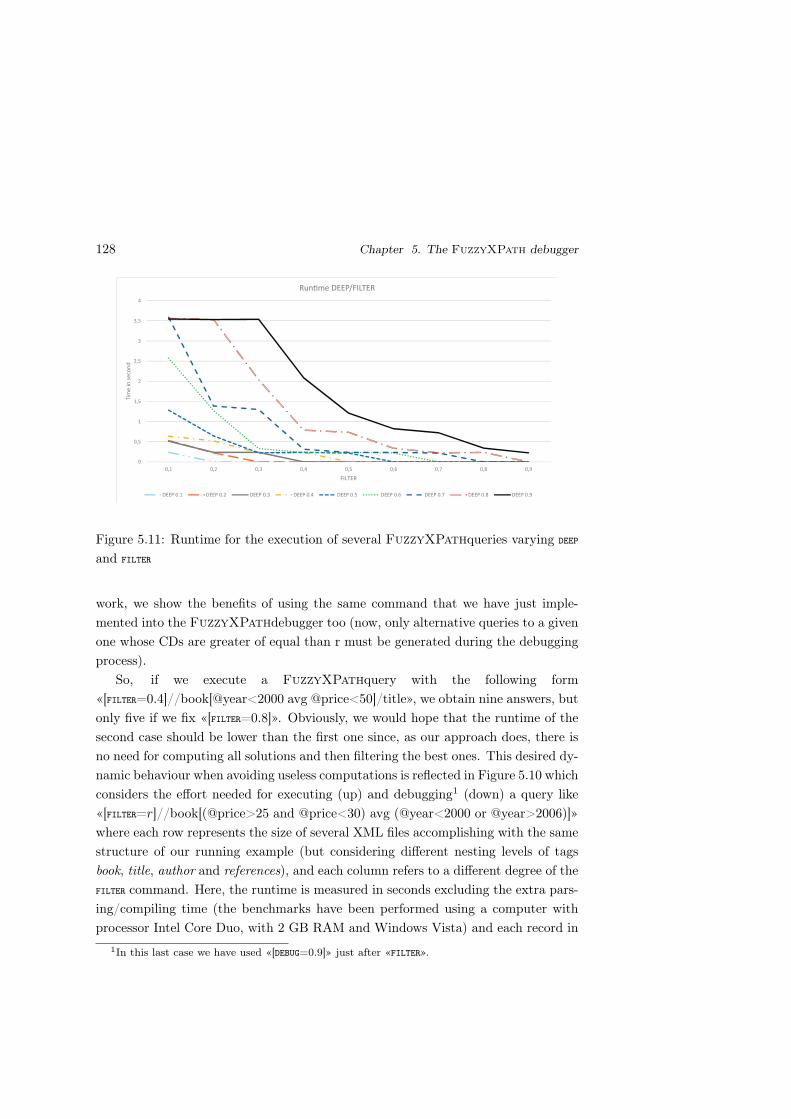
128 Chapter 5. The FuzzyXPath debugger
0
0,5
1
1,5
2
2,5
3
3,5
4
0,1 0,2 0,3 0,4 0,5 0,6 0,7 0,8 0,9
Tim
e i
n s
eco
nd
FILTER
Run e DEEP/FILTER
DEEP 0.1 DEEP 0.2 DEEP 0.3 DEEP 0.4 DEEP 0.5 DEEP 0.6 DEEP 0.7 DEEP 0.8 DEEP 0.9
Figure 5.11: Runtime for the execution of several FuzzyXPathqueries varying DEEP
and FILTER
work, we show the benefits of using the same command that we have just imple-
mented into the FuzzyXPathdebugger too (now, only alternative queries to a given
one whose CDs are greater of equal than r must be generated during the debugging
process).
So, if we execute a FuzzyXPathquery with the following form
«[FILTER=0.4]//book[@year<2000 avg @price<50]/title», we obtain nine answers, but
only five if we fix «[FILTER=0.8]». Obviously, we would hope that the runtime of the
second case should be lower than the first one since, as our approach does, there is
no need for computing all solutions and then filtering the best ones. This desired dy-
namic behaviour when avoiding useless computations is reflected in Figure 5.10 which
considers the effort needed for executing (up) and debugging1 (down) a query like
«[FILTER=r]//book[(@price>25 and @price<30) avg (@year<2000 or @year>2006)]»
where each row represents the size of several XML files accomplishing with the same
structure of our running example (but considering different nesting levels of tags
book, title, author and references), and each column refers to a different degree of the
FILTER command. Here, the runtime is measured in seconds excluding the extra pars-
ing/compiling time (the benchmarks have been performed using a computer with
processor Intel Core Duo, with 2 GB RAM and Windows Vista) and each record in
1In this last case we have used «[DEBUG=0.9]» just after «FILTER».

5.3. Dynamic Filters for the Thresholded Debugging of Queries 129
0
1
2
3
4
5
6
7
8
9
0,1 0,2 0,3 0,4 0,5 0,6 0,7 0,8 0,9
Tim
e i
n s
eco
nd
s
FILTER
Run!me DEBUG/FILTER
DEBUG 0,1 DEBUG 0,2 DEBUG 0,3 DEBUG 0,4 DEBUG 0,5 DEBUG 0,6 DEBUG 0,7 DEBUG 0,8 DEBUG 0,9
Figure 5.12: Runtime for the debugging of several FuzzyXPathqueries varying DEBUG
and FILTER
the input file refers to a different book (that is, the number of records coincides with
the number of occurrences of tag book) which might contain other books inside its
references tag. The size of the files in the figure moves from 323Kb (1000 records)
till 3223 Kb (10000 records), but our application works fine even when files of 33Mb
(100000 records), which reveals the interest of our results.
Moreover, in Figure 5.11 we continue with a similar query to the previous one,
but also considering the DEEP command2. Here, for a large XML document with a
fixed size, we express the number of seconds needed for executing such query when
varying FILTER and DEEP, where it is easy to see that the behaviour of the interpreter
is more and more improved whenever FILTER grows and DEEP decreases, as wanted. On
the other hand, Figure 5.12 reflects similar effects that occur in our debugger, where
the contrast now is established between the FILTER and DEBUG commands.
Although the core of our application is written with (fuzzy) MALP rules, our
implementation is based on the following items:
2This kind of statistics can be produced on-line for several XML files and
FuzzyXPathqueries via the following couple of URLs that we have just prepared
for the interested reader: http://dectau.uclm.es/fuzzyXPath/?q=FuzzyXPathStatistics and
http://dectau.uclm.es/fuzzyXPath/?q=DebugStatistics (regarding the interpreter and the debug-
ger, respectively).

130 Chapter 5. The FuzzyXPath debugger
(1) We have reused/adapted several modules of our previous Prolog-based im-
plementation of (crisp) XPath described in [Alm09, ABE08].
(2) We have used the SWI-Prolog library for loading XML files, in order to
represent a XML document by means of a Prolog term (the notion of term,
i.e. data structure, is just the same in MALP and Prolog).
(3) The parser of XPath has been extended to recognize the new keywords FILTER,
DEBUG, DEEP, DOWN, JUMP, avg, etc... with their proper arguments.
(4) Each tag is represented as a data-term of the form: element(Tag,Attribu-
tes,Subelements), where Tag is the name of the XML tag, Attributes is a Pro-
log list containing the attributes, and Subelements is a Prolog list containing
the sub-elements (i.e. sub-trees) of the tag. For instance, the XML document
used in our examples is represented in SWI-Prolog like:
[ element(bib,[],
[ element(name,[],[’Classic Literature’]),
element(book,[year=’2001’,price=’45.95’],
[ element(title,[],[’Don Quijote de la Mancha’]),
element(author,[],[’Miguel de Cervantes Saavedra’]),
element(references,[],
[ element(novel,[year=’1997’,price=’35.99’],
[ element(name,[],[’La Galatea’]),
element(author,[],[ ’Miguel de Cervantes Saavedra’]),
element(references,[],
[ element(book,[ year = ’1994’, price = ’25.99’],
[ element(title,[],[ ’Los trabajos de Persiles y Sigismunda’]),
element(author,[],[ ’Miguel de Cervantes Saavedra’])
])
])
])
])
]),
element(novel, [year=’1999’,price=’25.65’],
[ element(title,[],[’La Celestina’]),
element(author,[],[’Fernando de Rojas’])
])
])
]
Loading of documents is achieved by predicate load_xml(+File,-Term) and
writing by predicate write_xml(+File,+Term).
(5) Predicate fuzzyXPath(+ListXPath,+Tree,+Deep, +Down,+Filter,+Accum) re-
ceives six arguments: (1) ListXPath is the Prolog representation of a XPath

5.3. Dynamic Filters for the Thresholded Debugging of Queries 131
Figure 5.13: An on-line session with the FuzzyXPathdebugger
expression; (2) Tree is the term representing an input XML document; (3)
Deep/Down/Filter have the obvious meaning, and finally (4) the last argument
Accum (which is appropriately updated -maybe decreased- when going deeper
in the exploration of the file) accumulates the sequence of penalties produced
till reaching a concrete node, and it is very useful for deciding when perform-
ing a recursive call to the children of such node whenever the value of Accum
is better than the one fixed by Filter. These actions also directly revert on
the new predicate debugQuery (+ListXPath,+Tree,+Debug,+Filter,+Accum),
which implements the ideas described in this work and where once again the
appropriate management of the two last arguments becomes the keypoint of
our dynamic thresholding technique. Both the interpreter and the debug-
ger can be tested on-line via http://dectau.uclm.es/fuzzyXPath/?q=FuzzyXPathTest and
http://dectau.uclm.es/fuzzyXPath/?q=Debugger
XPathTest, respectively (see Figure 5.13).
(6) The evaluation of the query generates a truth value which has the form of a
tree, called tv tree. The main power of a fuzzy logic programming language like
MALP w.r.t. Prolog, is that instead of answering questions with a simple
true/false value, solutions are reported in a much more tinged, documented
way. Basically, the fuzzyXPath predicate traverses the Prolog tree represent-
ing a XML document annotating into the tv tree the corresponding DEEP/DOWN
values according to the movements performed in the horizontal and vertical
axis, respectively. In addition, the tv tree is annotated with the values of and,

132 Chapter 5. The FuzzyXPath debugger
or and avg operators in each node. For instance, the evaluation of the query
«/bib[DEEP=0.8]//book[@year<2000 avg3,1 @price<50]/title» generates the
following tv:
tv(1.0,[[],
tv(1.0,[[tv(0.25, [])],
tv(1.0,[element(title, [], [Don Quijote de la Mancha]), [], []]),
tv(1.0,[[],
tv(0.8,[[],
tv(0.8,[[],
tv(0.8,[[],
tv(0.8,[[tv(1.0, [])],
tv(1.0,[element(title, [], [Los trabajos de ...
....
For the case of the debugQuery predicate, it explores the XML tree in a very
similar way than the interpreter, but now the annotations performed on the
resulting tv tree refer to the corresponding JUMP, DELETE and SWAP values. For in-
stance, the tv tree associated to query «[DEBUG=0.5]//book/title» starts as:
tv(1.0,[[//, []],
tv(0.0,[[tag(noExist), []], [],
tv(0.5,[[[DELETE=0.5], [book=]],
tv(0.0,[[tag(noExist), []], [],
tv(0.0,[[tag(noExist), []], [],
tv(0.0,[[tag(noExist), []], [],
tv(0.5,[[[JUMP=0.5]//, [title= //]],
tv(0.9,[[tag(name), [title=name]], [],
tv(0.0,[[tag(noExist), []], [],
tv(0.0,[[tag(noExist), []], [], ...
....
(7) Finally, the tv tree is used for computing the output of the query, by multiplying
the recorded values. A predicate called tv_to_elem has been implemented to
output the answers in a sorted, pretty way.

Chapter 6
Applications
In this chapter we focus on the ability of FuzzyXPath for exploring derivation
trees generated by FLOPER once they are exported in XML format, which some-
how serves as a debugging/analizing tool for discovering the set of fuzzy computed
answers for a given goal, performing depth/breadth-first traversals of its associated
derivation tree, finding non fully evaluated branches, etc., thus reinforcing the bi-
lateral synergies between FuzzyXPath and FLOPER.
Then we deal with propositional fuzzy formulae containing several propositional
symbols linked with connectives defined in a lattice of truth degrees more complex
than Bool. Instead of focusing on satisfiability (i.e., proving the existence of at
least one model) as usually done in a SAT/SMT setting, our interest moves to the
problem of finding the whole set of models (with a finite domain) for a given fuzzy
formula. We re-use a previous method based on fuzzy logic programming where
the formula is conceived as a goal whose derivation tree, provided by our FLOPER
tool, contains on its leaves all the models of the original formula, together with other
interpretations. Next, we use the ability of the FuzzyXPath tool (developed in our
research group with FLOPER) for exploring these derivation trees once exported
in XML format, in order to discover whether the formula is a tautology, satisfiable,
or a contradiction.
133

134 Chapter 6. Applications
6.1 Exploring Derivation Trees with FuzzyXPath
Consider, for instance, the following with associated multi-adjoint lattice 〈[0, 1],R
,←P,&P〉 (where label P means for Product logic with the following connective
definitions for implication and conjunction symbols, respectively: “←P (x, y) =
min(1, x/y)”, “&P(x, y) = x ∗ y”, as well as “@aver(x, y) = (x+ y)/2”):
R1 : oc(X) <- s(X) &prod (f(X) @aver w(X)) with 1.
R2 : s(madrid) with 0.8. R5 : s(tokyo) with 0.9.
R3 : f(madrid) with 0.8. R6 : f(tokyo) with 0.7.
R4 : w(madrid) with 0.9. R7 : w(tokyo) with 0.6.
R8 : s(istambul) with 0.3. R11 : s(baku) with 0.3.
R9 : f(istambul) with 0.4. R12 : f(baku) with 0.2.
R10 : w(istambul) with 0.8. R13 : w(baku) with 0.5.
Figure 6.1: Execution tree for program P and goal oc(X)
This program models, through predicate oc/1, the chances of a city for being an
“olympic city” (i.e., for hosting olympic games). Predicate oc/1 is defined in rule

6.1. Exploring Derivation Trees with FuzzyXPath 135
R1, whose body collects the information from three other predicates, s/1, f/1 and
w/1, modeling, respectively, the security level, the f acilities and the good weather of
a certain city (other criteria like continental rotation, political/economical aspects,
etc... can be easily “aggregated” to the definition of oc/1). These predicates are
defined in rules R2 to R13 for four cities (Madrid, Istambul, Tokyo and Baku), in
such a way that, for each city, the feature modeled by each predicate is better the
greater the truth value of the rule.
The FLOPER system is able to manage programs with very different lattices. In
order to associate a certain lattice with its corresponding program, such lattice
must be loaded into the tool as a pure Prolog program. As an example, the following
clauses show the program modeling the lattice of the real interval [0, 1] with the usual
ordering relation and connectives (where the meaning of the mandatory predicates
member, top, bot and leq is obvious):
member(X):- number(X), 0=<X, X=<1. bot(0).
leq(X,Y):- X=<Y. top(1).
and_prod(X,Y,Z):- pri_prod(X,Y,Z). pri_prod(X,Y,Z):- Z is X * Y.
or_prod(X,Y,Z):- pri_prod(X,Y,U1),pri_add(X,Y,U2),pri_sub(U2,U1,Z).
pri_add(X,Y,Z):- Z is X+Y. pri_sub(X,Y,Z):- Z is X-Y.
FLOPER includes two main ways for evaluating a goal, given a MALP program
and its corresponding lattice. Option “run” translates the whole program into a pure
Prolog program and evaluates the (also translated) goal, thus obtaining a set of fuzzy
computed answers, whereas, on the other hand, option “tree” displays the execution
(or derivation) tree for the intended goal1. For the purpose of this chaper, we will
focus on this last option in order to obtain a tree (detailing the whole computational
behaviour) for being afterwards analyzed with FuzzyXPath.
Let us consider the previously described program P, and goal “oc(X)”, that asks
for the eligibility of each one of the four cities in P as “Olympic City”. We use option
“tree” to obtain the execution tree, which is generated by FLOPER in three differ-
ent formats. Firstly the tree is displayed in graphical mode, as a PNG file, as shown
in Figure 6.1. The tree is composed by two kinds of nodes. Yellow nodes represent
states reached by FLOPER following the state transition system that describes the
operational semantics of MALP [MOV04]. The up-most node represents the first
state (that is, the goal and the identity substitution), and subsequent lower nodes
are its children states (that is, states reached from the goal). A state contains a
1Users can select the deepest level to be built, which is obviously mandatory when trees are
infinite.

136 Chapter 6. Applications
formula in the upper side and a substitution (the record of substitutions applied
from the original goal to reach that state) at the bottom. A final state, if reached,
is a fuzzy computed answer, that is, its formula is an element of the lattice. Blue
rounded nodes that intermediate between a pair of yellow nodes (a pair of states)
represent program rules; specifically, the program rule that is exploited in order to
go from one state (the upper state) to another (the lower one). These rules are
named with letter “R” plus its position in the program. For example, observe that
from the initial state to the next state, rule R1 of the program has been exploited,
as shown in the blue intermediate node. As an exception, when all atoms have
been exploited in (the formula of) a certain state, the following blue node indicates
“result”, informing that the next state is a fuzzy computed answer.
FLOPER can also generate the execution tree in two textual formats. The
first one contains a plain description of the tree, while the second one provides an
XML structure to that description. In this XML format we define the tag “node”
to contain all the information of a node, such as the rule performed to reach that
state (that is “R0” in the case of the first state), the formula of the state, the ac-
cumulated substitution and the children nodes, given by the tags “rule”, “goal”,
“substitution” and “children”, respectively. The content of tags “rule”, “goal”
and “substitution” is a string, while the content of the tag “children” is a set of
tags “node”, as seen in the following lines, corresponding to the XML file associated
to the the tree depicted in Figure 6.1.

6.1. Exploring Derivation Trees with FuzzyXPath 137
<node>
<rule>R0</rule>
<goal>oc(X)</goal>
<substitution></substitution>
<children>
<node>
<rule>R1</rule>
<goal>and_prod(s(X),agr_aver(f(X),w(X)))</goal>
<substitution>X1/X</substitution>
<children>
<node>
<rule>R2</rule>
<goal>and_prod(0.8,agr_aver(f(madrid),w(madrid)))</goal>
<substitution>X/madrid,X1/madrid</substitution>
<children>
<node>
<rule>R3</rule>
<goal>and_prod(0.8,agr_aver(0.8,w(madrid)))</goal>
<substitution>X/madrid,X1/madrid</substitution>
<children>
<node>
<rule>R4</rule>
<goal>and_prod(0.8,agr_aver(0.8,0.9))</goal>
<substitution>X/madrid,X1/madrid</subtitution>
<children>
<node>
<rule>result</rule>
<goal>0.6800000000000002</goal>
<substitution>X/madrid,X1/madrid
</substitution>
<children>
</children>
</node>
</children>
</node>
</children>
</node>
</children>
</node>
...
<node>
<rule>result</rule>
<goal>0.585</goal>
<substitution>X/tokyo,X1/tokyo
</substitution>
<children>
</children>
</node>
...
</node>
</children>
</node>
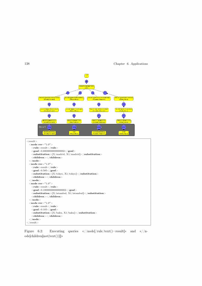
138 Chapter 6. Applications
<result>
<node rsv="1.0">
<rule>result</rule>
<goal>0.6800000000000002</goal>
<substitution>X/madrid, X1/madrid</substitution>
<children></children>
</node>
<node rsv="1.0">
<rule>result</rule>
<goal>0.585</goal>
<substitution>X/tokyo, X1/tokyo</substitution>
<children></children>
</node>
<node rsv="1.0">
<rule>result</rule>
<goal>0.18000000000000002</goal>
<substitution>X/istambul, X1/istambul</substitution>
<children></children>
</node>
<node rsv="1.0">
<rule>result</rule>
<goal>0.105</goal>
<substitution>X/baku, X1/baku</substitution>
<children></children>
</node>
</result>
Figure 6.2: Executing queries «//node[/rule/text()=result]» and «//n-
ode[children[not(text())]]»

6.1. Exploring Derivation Trees with FuzzyXPath 139
Now, we present a very powerful method to automatically exploring the be-
haviour of a MALP program using the FuzzyXPath tool described in Section 3.1.
The idea is to use FuzzyXPath over the execution tree generated by FLOPER
for a certain program and goal. That tree is obtained through option “tree” using
the XML format just explained before in Section 4.2. For instance, an easy but
interesting XPath query should be “//node/rule” which lists all the rules exploited
along the execution of a goal (in the case of the tree depicted in Figure 6.1, we would
obtain the whole set of rules defined in the program P of our running example).
Assume now that we plan to obtain the whole set of fuzzy computed answers for a
given goal and program. This information, always collected in the leaves of execution
trees (even when there exists the possibility of finding leaves non containing fuzzy
computed answers, as we will see afterwards) as illustrated in Figure 6.2, can be
retrieved by means of the FuzzyXPath query “//node[/rule/text()=result]”,
meaning that, return each node such that the content of its rule tag is “result”.
The XML text shown below Figure 6.2 represents the output of our FuzzyXPath
interpreter for that query, where the selected nodes have been highlighted inside a
blue cloud into the drawn tree above. Note that the resuting XML file contains four
solutions (one for each city), where attribute “rsv” indicates how much each city
fulfills the original query (in this example, this value is the same in all cases, that
is, just the maximum one 1).
Strongly related with the previous experiment, but not directly focusing now on fuzzy
computed answers, query “//node[children[not(text())]]” returns the leaves of
the tree. Note that, in the case of our current program P and goal “oc(X)”, the
corresponding output for this query is, once again, the same than the one reported
previously in Figure 6.2 but, as said in the previous paragraph, this is not the
general case. In fact, we can formulate a query like “//node[children[not(text())]
and rule/text()<> "result"]/goal”, helping us to know whether the tree has any
partially evaluated leaf (i.e., non reporting a fuzzy computed answer) since it returns
nodes at the end of a branch that are not labeled with the rule tag containing
“result”. The important meaning of this query resides on its capability for finding
possible sources of infinite loops. So, consider the example of Figure 6.4, where an
infinite branch (leaf in orange) is clearly observable between two leaves (in yellow)
containing fuzzy computed answers. This figure corresponds to the execution tree
(since it is infinite in depth, FLOPER allows us to fix the number of levels to be
drawn) for goal “p(X)” w.r.t. program:

140 Chapter 6. Applications
<result>
<goal rsv="1.0">oc(X)</goal>
<goal rsv="0.81">and_prod(s(X),agr_aver(f(X),w(X)))</goal>
<goal rsv="0.6561">and_prod(0.8,agr_aver(f(madrid),w(madrid)))</goal>
<goal rsv="0.6561">and_prod(0.9,agr_aver(f(tokyo),w(tokyo)))</goal>
<goal rsv="0.6561">and_prod(0.3,agr_aver(f(istambul),w(istambul)))</goal>
<goal rsv="0.6561">and_prod(0.3,agr_aver(f(baku),w(baku)))</goal>
<goal rsv="0.531441">and_prod(0.8,agr_aver(0.8,w(madrid)))</goal>
<goal rsv="0.531441">and_prod(0.9,agr_aver(0.7,w(tokyo)))</goal>
<goal rsv="0.531441">and_prod(0.3,agr_aver(0.4,w(istambul)))</goal>
<goal rsv="0.531441">and_prod(0.3,agr_aver(0.2,w(baku)))</goal>
</result>
Figure 6.3: Executing query «[FILTER=0.5][DEEP=0.9]//node/goal»
p(a) with 0.8.
p(X) <prod p(s(s(s(X)))) with 0.9.
p(b) with 0.6.
Note that, in this figure, the search for nodes with an empty “children” field by
using query “//node[children[not(text())]]/goal” returns three solutions, i.e.,
the three leaves of the tree without distinguishing whether they correspond to fully
or partially evaluated goals. Query “//node[rule/text()="result"]/goal” allows
us to retrieve only the fca’s of the tree, as seen in Figure 6.4. Finally, in order to

6.1. Exploring Derivation Trees with FuzzyXPath 141
Executing query «//node[children[not(text())]]/goal»<result>
<goal>0.4</goal>
<goal>agr_aver(0,and_prod(0.9,...p(s(...(s(X))))))</goal>
<goal>0.3</goal>
</result>
Executing query «//node[children[not(text())] and rule/text()<>“result”]/goal»<result>
<goal>agr_aver(0,and_prod(0.9,...p(s(...(s(X))))))</goal>
</result>
Executing query «//node[rule/text()=“result”]/goal»<result>
<goal>0.4</goal>
<goal>0.3</goal>
</result>
Figure 6.4: Example of tree with an infinite branch
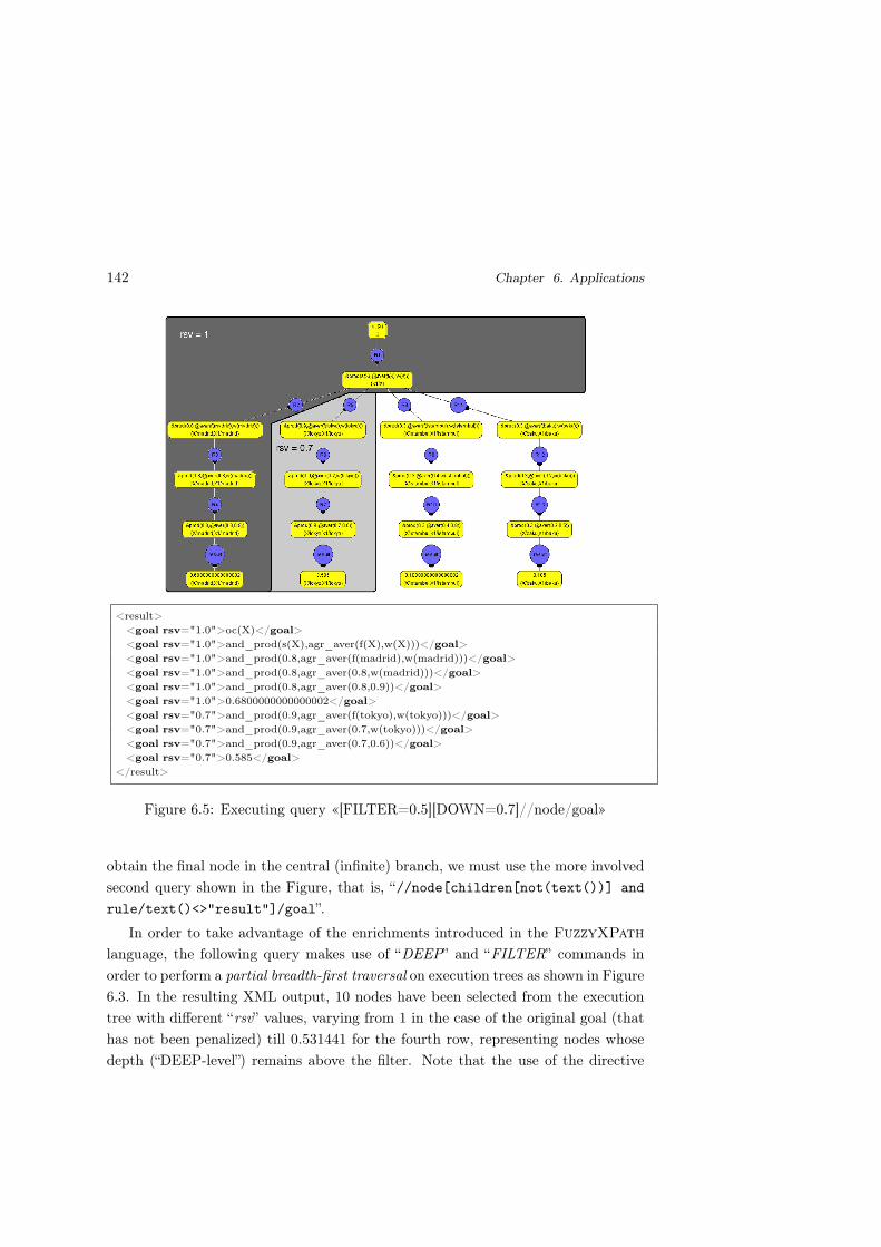
142 Chapter 6. Applications
<result>
<goal rsv="1.0">oc(X)</goal>
<goal rsv="1.0">and_prod(s(X),agr_aver(f(X),w(X)))</goal>
<goal rsv="1.0">and_prod(0.8,agr_aver(f(madrid),w(madrid)))</goal>
<goal rsv="1.0">and_prod(0.8,agr_aver(0.8,w(madrid)))</goal>
<goal rsv="1.0">and_prod(0.8,agr_aver(0.8,0.9))</goal>
<goal rsv="1.0">0.6800000000000002</goal>
<goal rsv="0.7">and_prod(0.9,agr_aver(f(tokyo),w(tokyo)))</goal>
<goal rsv="0.7">and_prod(0.9,agr_aver(0.7,w(tokyo)))</goal>
<goal rsv="0.7">and_prod(0.9,agr_aver(0.7,0.6))</goal>
<goal rsv="0.7">0.585</goal>
</result>
Figure 6.5: Executing query «[FILTER=0.5][DOWN=0.7]//node/goal»
obtain the final node in the central (infinite) branch, we must use the more involved
second query shown in the Figure, that is, “//node[children[not(text())] and
rule/text()<>"result"]/goal”.
In order to take advantage of the enrichments introduced in the FuzzyXPath
language, the following query makes use of “DEEP” and “FILTER” commands in
order to perform a partial breadth-first traversal on execution trees as shown in Figure
6.3. In the resulting XML output, 10 nodes have been selected from the execution
tree with different “rsv” values, varying from 1 in the case of the original goal (that
has not been penalized) till 0.531441 for the fourth row, representing nodes whose
depth (“DEEP-level”) remains above the filter. Note that the use of the directive

6.1. Exploring Derivation Trees with FuzzyXPath 143
“DEEP” segregates the nodes of the tree from top to bottom, since lower nodes in
the tree are represented deeper in the input XML file.
<result>
<goal rsv="1.0">and_prod(0.3,agr_aver(f(istambul),w(istambul)))</goal>
<goal rsv="1.0">and_prod(0.3,agr_aver(0.4,w(istambul)))</goal>
<goal rsv="0.6667">and_prod(0.3,agr_aver(0.4,0.8))</goal>
<goal rsv="0.6667">0.18000000000000002</goal>
<goal rsv="0.3333">and_prod(s(X),agr_aver(f(X),w(X)))</goal>
<goal rsv="0.3333">and_prod(0.8,agr_aver(f(madrid),w(madrid)))</goal>
<goal rsv="0.3333">and_prod(0.9,agr_aver(f(tokyo),w(tokyo)))</goal>
<goal rsv="0.3333">and_prod(0.3,agr_aver(f(baku),w(baku)))</goal>
<goal rsv="0.3333">and_prod(0.8,agr_aver(0.8,w(madrid)))</goal>
<goal rsv="0.3333">and_prod(0.9,agr_aver(0.7,w(tokyo)))</goal>
<goal rsv="0.3333">and_prod(0.3,agr_aver(0.2,w(baku)))</goal>
</result>
Figure 6.6: Execution of the query «node[/goal[contains(text(),“w(”)] aver1,2 substi-
tution[contains(text(),“istambul”)]]//goal»
Analogously, in Figure 6.5 we use “DOWN” instead of “DEEP” for producing partial
depth-first traversals on execution trees. In this case, our query segregates the nodes
from left to right in columns, since the more left the node appears in the tree, the
upper is it in the XML output and, thus, the less penalized by “DOWN”. As previously,
10 nodes have been selected again with “rsv” ranging from 1 -upper nodes in the
XM file- in the left column, till 0.7, as shown in the second column.

144 Chapter 6. Applications
In order to illustrate the high expressive power of the FuzzyXPath language,
in the following we try to model queries joining several concepts (for instance, the
topics of “weather” and “Istambul” modeled in P as predicate “w” and constant
“istambul”, respectively). Assume that we are firstly interested on nodes informing
about “weather”, i.e., focusing on the fourth rows of our execution tree, thus meaning
that sub-string “w(” must appear in tag “goal”, while our second preference asks for
nodes in the branch containing the word “istambul” in tag “substitution”. In order to
join these two constraints, instead of using crisp “or/and” operators (or even different
fuzzy variants of such connectives already implemented in FuzzyXPath), we prefer
to use an arithmetical average giving twice importance to the second requirement
than to the first one. The FuzzyXPath formulation of our query entitles Figure 6.6,
where we graphically show the set of solutions as well as the output in the resulting
XML file.
6.2 FuzzyXPath for the Automatic Search of Fuzzy
Formulae Models
Research on SAT (Boolean Satisfiability) and SMT (Satisfiability Modulo Theo-
ries) [BSST09] represents a successful and large tradition in the development of
highly efficient automatic theorem solvers for classic logic. More recently there also
exist attempts for covering fuzzy logics, as occurs with the approaches presented
in [ABMV12, VBG12]. Moreover, if automatic theorem solving supposes too a
starting point for the foundations of logic programming as well as one of its impor-
tant application fields [Llo87, Sti88, Bra00, Apt90], in [BMVV13] we showed some
preliminary guidelines about how fuzzy logic programming [KS92, Ger01, AF02,
MOV04, MCS11] can face the automatic proving of fuzzy theorems by making use
of the FLOPER environment .
Let us start our discussion with an easy motivating example. Assume that we
have a very simple digital chip with just a single input port and just one output
port, such that it reverts on Out the signal received from In. The behaviour of such
chip can be represented by the following propositional formula F : (¬In ∧ Out) ∨(In ∧ ¬Out). Depending on how we interpret each propositional symbol, we obtain
the following final set of interpretations for the whole formula:
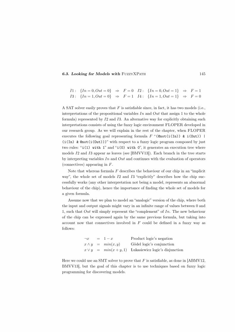
6.3. Looking for Models with FuzzyXPath 145
I1 : In = 0, Out = 0 ⇒ F = 0 I2 : In = 0, Out = 1 ⇒ F = 1
I3 : In = 1, Out = 0 ⇒ F = 1 I4 : In = 1, Out = 1 ⇒ F = 0
A SAT solver easily proves that F is satisfiable since, in fact, it has two models (i.e.,
interpretations of the propositional variables In and Out that assign 1 to the whole
formula) represented by I2 and I3. An alternative way for explicitly obtaining such
interpretations consists of using the fuzzy logic environment FLOPER developed in
our research group. As we will explain in the rest of the chapter, when FLOPER
executes the following goal representing formula F “(@not(i(In)) & i(Out)) |
(i(In) & @not(i(Out)))” with respect to a fuzzy logic program composed by just
two rules: “i(1) with 1” and “i(0) with 0”, it generates an execution tree where
models I2 and I3 appear as leaves (see [BMVV13]). Each branch in the tree starts
by interpreting variables In and Out and continues with the evaluation of operators
(connectives) appearing in F .
Note that whereas formula F describes the behaviour of our chip in an “implicit
way”, the whole set of models I2 and I3 “explicitly” describes how the chip suc-
cessfully works (any other interpretation not being a model, represents an abnormal
behaviour of the chip), hence the importance of finding the whole set of models for
a given formula.
Assume now that we plan to model an “analogic” version of the chip, where both
the input and output signals might vary in an infinite range of values between 0 and
1, such that Out will simply represent the “complement” of In. The new behaviour
of the chip can be expressed again by the same previous formula, but taking into
account now that connectives involved in F could be defined in a fuzzy way as
follows:
¬x = 1− x Product logic’s negation
x ∧ y = min(x, y) Gödel logic’s conjunction
x ∨ y = min(x+ y, 1) Łukasiewicz logic’s disjunction
Here we could use an SMT solver to prove that F is satisfiable, as done in [ABMV12,
BMVV13], but the goal of this chapter is to use techniques based on fuzzy logic
programming for discovering models.

146 Chapter 6. Applications
member(bottom). member(alpha).
member(beta). member(top).
members([bottom,alpha,beta,top]).
leq(bottom,X). leq(alpha,alpha).
leq(beta,beta). leq(X,top).
and_godel(X,Y,Z) :- pri_inf(X,Y,Z).
pri_inf(bottom,X,bottom):-!.
pri_inf(alpha,X,alpha):-leq(alpha,X),!.
pri_inf(beta,X,beta):-leq(beta,X),!.
pri_inf(top,X,X):-!.
pri_inf(X,Y,bottom).
Figure 6.7: Lattice of truth degrees F modeled in Prolog.
6.3 Looking for Models with FuzzyXPath
The subset of the MALP language detailed in Section 2.2 suffices for developing a
simple fuzzy theorem prover, where it is important to remark that our tool can cope
with different lattices (not only the real interval [0,1]) containing a finite number of
elements -marked in “members”- maintaining full or partial ordering among them.
Hence, we can use FLOPER for enumerating the whole set of interpretations and
models of fuzzy formulae. To this end, only a concrete lattice L is required in
order to automatically build a program composed by a set of facts of the form
“i(α) with α”, for each α ∈ L. For instance, the MALP program associated to
lattice F in Figure 6.7 looks like:
i(top) with top.
i(alpha) with alpha.
i(beta) with beta.
i(bottom) with bottom.

6.3. Looking for Models with FuzzyXPath 147
Once the lattice and the residual program have been loaded into FLOPER, the
formula to be evaluated is introduced as a goal to the system following some con-
ventions:
• If P is a propositional variable in the original formula, then it is denoted as
“i(P)” in the goal F .
• If & is a conjunction of a certain logic “label” in the original formula, then it
is denoted as “&label” in goal F .
• For disjunctions, negations and implications, use respectively the patterns
“ |label”, “@no_label” and “@im_label” in F .
• For other aggregators use “@label” in F .
In what follows we discuss some examples related with the lattice shown in Figure 6.7
and its residual MALP program just seen before. Firstly, if we execute goal “i(P)”
into FLOPER, we obtain the four interpretations for P shown in Figure 6.8. On
the other hand, consider now the propositional formula P ∨ Q, which is translated
into the MALP goal “(i(P) | i(Q))” and after being executed with FLOPER,
the tool returns a tree as seen in Figure 6.9 whose 16 leaves represent the whole
set of interpretations, where 9 of them -inside blue clouds- are models (see part
of the corresponding XML file produced by FLOPER in Figure 6.10). Here, each
state contains its corresponding goal and substitution components and they are
drawn inside yellow circles. Admissible steps, coloured in blue, are labelled with
the program rule they exploit. Finally, those blue circles annotated with word “is”,
correspond to interpretive steps. Sometimes we include blue circles labelled with
“result” which represents a chained sequence of interpretive steps.
With our FuzzyXPath tool we have executed “//node[goal=’top’]/sub”
against the XML file shown in Figure 6.10, which was generated by FLOPER
when producing the proof tree drawn in Figure 6.9, thus returning as output the
new XML document listed in Figure 6.11. As illustrated in Figure 6.10, note that
the XML files representing proof trees exported by FLOPER, are always rooted
with the node label, whose children are based on four kinds of ‘tags’ (this structure
is nested as much as needed):
• rule, which indicates the program rule exploited to reach the current node
(the virtual rule R0 is pointed out only in the initial node),

148 Chapter 6. Applications
Figure 6.8: A work-session with FLOPER solving goal i(P).
• goal, which contains the MALP expression under evaluation, that is, the for-
mula that the system is trying to prove on its current initial/intermediate/final
step. Note that, when in our example such value is top, then we have found a
model, where the values assigned to the propositional symbols of the formula
are collected in the following tag...
• sub, acronym of “substitution”, which accumulates the variable bindings per-
formed along a fuzzy logic derivation (i.e., chain of computational steps along a
branch of the execution tree) and whose meaning in our target setting, reveals
the way of interpreting the propositions contained on a formula for obtaining
its models. See for instance Figure 6.11, where the nine solutions labeled with
this tag and reported in the output XML document, indicate each one the
truth values for the propositional variables that satisfy the formula with the
maximum truth degree. And finally,

6.3. Looking for Models with FuzzyXPath 149
Figure 6.9: A work-session with FLOPER solving formula P∨Q (16 interpretations,
9 models).
• children, which contains the set of underlying nodes of the tree in a nested
way.
Consider now the more involved formula P ∧ Q → P ∨ Q which becomes into
the MALP goal “(i(P) & i(Q)) @impl (i(P) | i(Q))”. When interpreted by
FLOPER, the system returns a list of answers having all them the maximum truth
degree “top”, which proves that this formula is a tautology, as wanted. Assume now
a more general version with the following shape Fn = P1 ∧ . . .∧Pn → P1 ∨ . . .∨Pn.
With respect to the efficiency of the method presented here, we have studied the be-
haviour of formula Fn in the table of Figure 6.12. In the horizontal axis we represent
the number n of different propositional variables appearing in the formula, whereas
the vertical axis refers to the number of seconds needed to obtain the whole set of
interpretations (all them are models in this case) for the formula. The benchmarks
have been performed using a computer with processor Intel Core Duo, with 2 GB
RAM and Windows Vista. Both the red and blue lines refers to the method just
commented along this chapter, but whereas the red line indicates that the derivation
tree has been produced by performing admissible and interpretive steps according
Definitions 2.1.2 and 2.1.5, respectively, the blue line refers to the execution of the
Prolog code obtained after compiling with FLOPER the MALP program and goal
associated to our intended formula.
The results achieved in Figure 6.12 show that our method has a nice behaviour
in both cases, even for formulae with a big number of propositional variables. Of
course, the method does not try to compete with SAT techniques (which are always
faster and can deal with more complex formulae containing many more propositional
variables), but it is important to remark again that in our case, we face the problem

150 Chapter 6. Applications
<node>
<rule>R0</rule>
<goal>or_godel(i(P),i(Q))</goal>
<substitution></sub>
<children>
<node>
<rule>R1</rule>
<goal>or_godel(bottom,i(Q))</goal>
<sub>P/bottom</sub>
<children>
<node>
<rule>R1</rule>
<goal>or_godel(bottom,bottom)</goal>
<sub>Q/bottom,P/bottom
</sub>
<children>
<node>
<rule>result</rule>
<goal>bottom</goal>
<sub>Q/bottom,P/bottom
</sub>
<children>
</children>
</node>
</children>
</node>
...
Figure 6.10: Part of the XML file representing the execution tree shown in Figure
6.9.
of finding the whole set of models for a given formula, instead of only focusing on
satisfiability.
We address now formula Fn because it illustrates one key point of this chapter.
Note that there are |L|n interpretations for that formula, where |L| is the cardinality
of the carrier set of lattice L that models truth degrees. For our example lattice of
Figure 6.7, with four elements, we have 4n interpretations. Consider, for example,
that we are interested in proving that a certain formula, say F5, is a tautology. In
[BMVV13] we would have to search at least one interpretation that is not model of F5
to prove that it is not a tautology, but since there exist 45 = 1024 interpretations,
this task is not suitable to be made by hand. To overcome this problem we use

6.3. Looking for Models with FuzzyXPath 151
<result>
<sub rsv=1>Q/top,P/top</sub>
<sub rsv=1>Q/alpha,P/top</sub>
<sub rsv=1>Q/beta,P/top</sub>
<sub rsv=1>Q/bottom,P/top</sub>
<sub rsv=1>Q/top,P/alpha</sub>
<sub rsv=1>Q/beta,P/alpha</sub>
<sub rsv=1>Q/top,P/beta</sub>
<sub rsv=1>Q/alpha,P/beta</sub>
<sub rsv=1>Q/top,P/bottom</sub>
</result>
Figure 6.11: XML file obtained after evaluating an XPath query.
FuzzyXPath to automatically search in the XML file generated by FLOPER.
The manual task, then, is reduced to designing the FuzzyXPath query. In this
case, since we are interested in proving that F5 is a tautology, our FuzzyXPath
query should be //node[rule=‘result’ & goal<>‘top’]/sub, that is, the system
searches nodes whose rule tag contain the text “result” (i.e., we are looking for
leaves in the tree) and whose tag goal is not “top” (in order to exclude models). If
the output of this query is an empty list of nodes, as it actually is, the formula F5
is proven to be a tautology, as desired.
FuzzyXPath can also be used for determining the satisfiability of a formula.
Consider again formula P ∨Q whose set of interpretations are shown in Figure 6.9.
The query //node[rule=‘result’ & goal<>‘top’]/sub seen above, shows that
this formula is not a tautology, since its further evaluation returns the non-empty
set:
<result>
<sub rsv=1>Q/alpha,P/alpha</sub>
<sub rsv=1>Q/bottom,P/alpha</sub>
<sub rsv=1>Q/beta,P/beta</sub>
<sub rsv=1>Q/bottom,P/beta</sub>
<sub rsv=1>Q/alpha,P/bottom</sub>
<sub rsv=1>Q/beta,P/bottom</sub>
<sub rsv=1>Q/bottom,P/bottom</sub>
</result>
Consider now the new query (which is almost antagonist to the previous one)
//node[rule=‘result’ & goal=‘top’]/sub. In this case, if the output is the

152 Chapter 6. Applications
Figure 6.12: Efficiency of the method.
empty set, the tested formula is a contradiction (i.e., there is no interpretation
satisfying it). Otherwise, it is satisfiable. Furthermore, with FuzzyXPath we can
come back to the main purpose of [BMVV13], that is listing the set of models of a
formula instead of just deciding whether it is satisfiable or not. In particular, the
query to list the set of models is the one presented for deciding the satisfiability of
the formula at the beginning of this paragraph. Observe in Figure 6.11 the output
of this query w.r.t. formula P ∨Q.
Until now we have made use of FuzzyXPath to decide immediately the satisfia-
bility or not of a certain formula. With respect to the queries we have presented, we
were interested only in whether their answer set were empty or not. Now we present
a query which, by making use of the fuzzy capabilities of FuzzyXPath, returns the
list of interpretations together with extra information (into the rsv attribute) about
the extent in which they satisfy the formula or not. Consider again formula P ∨Q,
part of whose derivation tree is represented in the form of the XML file provided by
FLOPER in Figure 6.10. This formula is satisfiable but not a tautology, that is,

6.3. Looking for Models with FuzzyXPath 153
some of its interpretations satisfy it but other ones do not.
Let us focus now on query //node[rule=‘result’&(goal=‘top’ avg3,1,
goal<>‘top’)]/sub for such formula. Here, we ask for those states which are
leaves of the tree (condition rule=‘result’) and which are either models (con-
dition goal=‘top’) or not (condition goal<>‘top’), with the particularity that if
the leaf is a model, it fulfils the query at a 75% and, if it is not, with a 25%. The
result is the set of interpretations with a rsv value (the degree in which they fulfil
the query) between 0.75 and 0.25, as shown in the following table:
<result>
<sub rsv=0.75>Q/top,P/top</sub>
<sub rsv=0.75>Q/alpha,P/top</sub>
<sub rsv=0.75>Q/beta,P/top</sub>
<sub rsv=0.75>Q/bottom,P/top</sub>
<sub rsv=0.75>Q/top,P/alpha</sub>
<sub rsv=0.75>Q/beta,P/alpha</sub>
<sub rsv=0.75>Q/top,P/beta</sub>
<sub rsv=0.75>Q/alpha,P/beta</sub>
<sub rsv=0.75>Q/top,P/bottom</sub>
<sub rsv=0.25>Q/alpha,P/alpha</sub>
<sub rsv=0.25>Q/bottom,P/alpha</sub>
<sub rsv=0.25>Q/beta,P/beta</sub>
<sub rsv=0.25>Q/bottom,P/beta</sub>
<sub rsv=0.25>Q/alpha,P/bottom</sub>
<sub rsv=0.25>Q/beta,P/bottom</sub>
<sub rsv=0.25>Q/bottom,P/bottom</sub>
</result>
This set of answers briefly show the set of interpretations of the formula. For formulas
like F5, whose XML file of 5.5 MB would be impossible to check by hand, this method
offers a quick look of the answers, even when they are very numerous.

154 Chapter 6. Applications
Chapter 7
Conclusions and Future Work
In this thesis we have described the foundations and implementation of a flexible
extension based on fuzzy logic programming of the well-known XPath language. The
new FuzzyXPath dialect takes profit of the underlying source MALP language for
easily modeling a wide range of flexible operators representing different versions of
conjunctions, disjunctions and other highly expressive hybrid operators for retrieving
data from XML documents, as well as for constraining queries with structural and
thresholding conditions. We have shown with examples how FuzzyXPath is able to
express queries in which user preferences are encoded as combination of the defined
flexible operators, as well as how the language ranks answers according to them.
We have described the implementation which has been coded as a set of MALP
rules developed under the FLOPER system. We have shown how the operators
defined in FuzzyXPath have a correspondence in MALP, and how MALP is used
to compute ranked answers. The main element of the implementation is the adoption
of truth value trees for representing truth values in each node of an XML tree, which
are used to compute the retrieval status value of each answer.
Moreover, FuzzyXPath has been integrated in the MALP framework by pro-
viding semantics to fuzzy logic programs that work with trees with truth values.
This has required to study the semantics of trees with truth values and operations
on them in the context of multi-adjoint logic programming.
Additionally, we have studied an XQuery based implementation of our proposed
FuzzyXPath . An XQuery library has been implemented enabling the execution of
FuzzyXPath expressions in an XQuery interpreter. The implementation in XQuery
155
156 Chapter 7. Conclusions and Future Work
of FuzzyXPath required to introduce fuzzy connectives in the Boolean language
XQuery, as well as represent and work with trees with truth values in XQuery.
We have also studied an approach for XPath debugging. The result of the debug-
ging process of a XPath expression is a set of alternative queries, each one associated
to a chance degree. We have proposed JUMP, DELETE and SWAP operators that cover the
main cases of programming errors when describing a path about a XML document.
Our implemented and tested approach has a fuzzy taste in the sense that XPath
expressions are debugged by relaxing the shape of path queries with chance degrees.
Our debugging technique gives to programmers a chance degree for each proposed
alternative by annotating wrong-points on XPath expressions.
With regard to performance of the proposed FuzzyXPath language, a fuzzy
command for filtering the set of ranked answers in a dynamic way has been studied, in
order to reduce the runtime and complexity of computations when dealing with large
files. Our idea was to create filters for prematurely disregarding those superfluous
computations dealing with non-significant solutions. We have shown benchmarks of
performance of our system, improved by dynamic filtering.
Additionally, we have shown the mutual benefits between two different fuzzy
tools developed in our research group, that is, the FLOPER programming environ-
ment and the FuzzyXPath interpreter. Initially FLOPER was conceived as a tool
for implementing flexible software applications -as it is the case of FuzzyXPath-
coded with the fuzzy logic language MALP and offering options for compiling fuzzy
rules to standard Prolog clauses, running goals and drawing execution trees. Such
trees, once modeled in XML format inside the proper FLOPER tool, can be then
analyzed by the FuzzyXPath interpreter in order to discover details (such as fuzzy
computed answers, possible infinite branches and so on) of the computational be-
havior of MALP programs after being executed into FLOPER. Moreover, we have
applied this last capability of FuzzyXPath focusing exclusively on derivation trees
associated to fuzzy formulae. As a result, we have presented an automatic technique
useful for determining important features of such formulae (tautology, contradiction,
etc...) by making use of XPath queries with a fuzzy taste.
As future work we plan the following research lines. Firstly, we are interested to
extend our FuzzyXPath with the handling of text content in the same line as Full-
text XPath [CDH+11]. In our current proposal, a string used in a query has exactly
mach to the content of a node to be included in the answer. Full text XPath makes
possible to use “fuzzy” versions of string matching to which an score is associated.

157
String comparison techniques have been largely studied in many other contexts, and
they can be adapted to our work.
Also, we would like to extend our FuzzyXPath with other fuzzy logic mechanism
(vagueness, similarity, among others). Path and content matching in our proposed
FuzzyXPath are merely syntactic, however using vague concepts and enabling sim-
ilarity can lead to better results. In this line, we also find that MALP and FLOPER
can be used in ontologies and the Semantic Web, following [Str05b, LS08, For11],
making possible a semantic based matching of paths and content.
Additionally, we are interested in top-k answering. Top-k answering has been al-
ready studied for fuzzy logic programming [SM12], and can be adapted to FLOPER.
Top-k answering determines the top k answers to a query without computing the
-usually wider, possibly infinite- whole set of solutions, which is strongly related with
the FILTER command.
Finally, we are interested to incorporate more mechanisms of searching, rank-
ing, debugging and filtering to the standard XQuery language. Extensions of the
proposed XQuery library can be implemented in the future to include other fuzzy
mechanisms (vagueness, similarity, etc), as well as XQuery debugging (JUMP, DELETE
and SWAP), and filtering (including Top-k answering).

158 Chapter 7. Conclusions and Future Work

Bibliography
[ABE08] J. M. Almendros-Jiménez, A. Becerra-Terón, F. J. Enciso-Baños. Query-
ing XML documents in Logic Programming. Theory and Practice of Logic
Programming 8(3):323–361, 2008.
[ABL+15] J. M. Almendros-Jiménez, M. Bofill, A. Luna, G. Moreno, C. Vázquez,
M. Villaret. Fuzzy XPath for the Automatic Search of Fuzzy Formulae
Models. In Scalable Uncertainty Management - 9th International Confer-
ence, SUM 2015, Québec City, QC, Canada, September 16-18, 2015. Pro-
ceedings. Pp. 385–398. Springer LNCS, 2015.
[ABMV12] C. Ansótegui, M. Bofill, F. Manyà, M. Villaret. Building Automated
Theorem Provers for Infinitely-Valued Logics with Satisfiability Modulo
Theory Solvers. In Proceedings of the 42nd IEEE International Symposium
on Multiple-Valued Logic, ISMVL 2012. Pp. 25–30. 2012.
[Ack67] R. Ackerman. Introduction to Many Valued Logics. Dover, New York, 1967.
[ACT95] C. Alsina, J. L. Castro, E. Trillas. On the characterization of S and R
implications. In Proc. of the 6th International Fuzzy Systems Association
World Congress, Sao Paulo. Volume 1, pp. 317–319. 1995.
[Acz48] J. Aczél. On mean values. Bulletin of the American Mathematical Society
54(2):392–400, 1948.
[Ada76] J. B. Adams. Probabilistic reasoning and certainty factors. Mathematical
Biosciences 32:177–186, 1976.
[AF99] F. Arcelli, F. Formato. Likelog: A Logic Programming Language for Flex-
ible Data Retrieval. In Proc. of the ACM Symposium on Applied Comput-
159

160 BIBLIOGRAPHY
ing, SAC’99, San Antonio. Pp. 260–267. ACM, Artificial Intelligence and
Computational Logic, 1999.
[AF02] F. Arcelli, F. Formato. A similarity-based resolution rule. International
Journal of Intelligent Systems 17(9):853–872, 2002.
[AG93] K. Atanassov, C. Georgiev. Intuitionistic fuzzy Prolog. Fuzzy Sets Systems
53(2):121–128, 1993.
[AG98] T. Alsinet, L. Godo. Fuzzy Unification Degree. In Proc. 2th International
Workshop on Logic Programming and Soft Computing’98, in conjunction
with JICSLP’98, Manchester. P. 18. 1998.
[Alm09] J. M. Almendros-Jiménez. An Encoding of XQuery in Prolog. In Pro-
ceedings of the Sixth International XML Database Symposium XSym’09.
Pp. 145–155. Springer, Lecture Notes in Computer Science 5679, Heildel-
berg, Germany, 2009.
[ALM11a] J. Almendros-Jiménez, A. Luna, G. Moreno. A Flexible XPath-based
Query Language Implemented with Fuzzy Logic Programming. In Bassil-
iades et al. (eds.), Proc. of 5th International Symposium on Rules: Re-
search Based, Industry Focused, RuleML’11. Barcelona, Spain, July 19–21.
Pp. 186–193. Springer Verlag, Lectures Notes in Computer Science 6826,
2011.
[ALM11b] J. Almendros-Jiménez, A. Luna, G. Moreno. Fuzzy Logic Programming
for Implementing a Flexible XPath-based Query Language. In Arenas et al.
(eds.), Proc. of XI Jornadas sobre Programación y Lenguajes, PROLE’11,
A Coruña, Spain, September 5-7. Pp. 154–168. Universidade da Coruña
(ISBN 978-84-9749-487-8), 2011.
[ALM12a] J. Almendros-Jiménez, A. Luna, G. Moreno. A XPath Debugger based
on Fuzzy Chance Degrees. In Herrero et al. (eds.), On the Move to Mean-
ingful Internet Systems: OTM 2012 Workshops, Rome, Italy, September
10-14, 2012. Proceedings. Pp. 669–672. Springer Verlag, Lectures Notes in
Computer Science 7567, 2012.
[ALM12b] J. Almendros-Jiménez, A. Luna, G. Moreno. Debugging Fuzzy XPath
Queries. In Gallardo et al. (eds.), Actas de las XII Jornadas sobre Progra-
mación y Lenguajes, PROLE’12, Jornadas SISTEDES, Almería, Spain,

BIBLIOGRAPHY 161
September 17-19. Pp. 119–133 (sección de trabajos en progreso). Universi-
dad de Almería (ISBN:978-84-15487-27-2), 2012.
[ALM12c] J. Almendros-Jiménez, A. Luna, G. Moreno. Fuzzy Logic Programming
for Implementing a Flexible XPath-based Query Language. Electronic
Notes in Theoretical Computer Science 282:3–18, 2012. Extended version
of [ALM11b].
[ALM13] J. Almendros-Jiménez, A. Luna, G. Moreno. Annotating Fuzzy Chance
Degrees when Debugging XPath Queries. In Advances in Computational
Intelligence - Proc of the 12th International Work-Conference on Artifi-
cial Neural Networks, IWANN 2013 (Special Session on Fuzzy Logic and
Soft Computing Application), Tenerife, Spain, June 12-14. Pp. 300–311.
Springer Verlag, LNCS 7903, Part II, 2013.
[ALM14a] J. M. Almendros-Jiménez, A. Luna, G. Moreno. Dynamic Filtering of
Ranked Answers When Evaluating Fuzzy XPath Queries. In Cornelis
et al. (eds.), Rough Sets and Current Trends in Computing - 9th Interna-
tional Conference, RSCTC 2014, Granada and Madrid, Spain, July 9-13,
2014. Proceedings. Lecture Notes in Computer Science 8536, pp. 319–330.
Springer International Publishing, 2014.
http://dx.doi.org/10.1007/978-3-319-08644-6_33
[ALM14b] J. M. Almendros-Jiménez, A. Luna, G. Moreno. Fuzzy XPath Queries in
XQuery. In On the Move to Meaningful Internet Systems: OTM 2014 Con-
ferences - Confederated International Conferences: CoopIS, and ODBASE
2014, Amantea, Italy, October 27-31, 2014, Proceedings. Pp. 457–472.
2014.
[ALM15a] J. M. Almendros-Jiménez, A. Luna, G. Moreno. Fuzzy XPath through
Fuzzy Logic Programming. New Generation Comput. 33(2):173–209, 2015.
[ALM15b] J. M. Almendros-Jiménez, A. Luna, G. Moreno. Thresholded Debugging
of XPath Queries. In Proc. of the 2015 IEEE International Conference on
Fuzzy Systems, FUZZIEEE’15. Istanbul, Turkey, August 2-5, 2015, Pages
9. 2015.
[ALMV13] J. M. Almendros-Jiménez, A. Luna, G. Moreno, C. Vázquez. Analyz-
ing Fuzzy Logic Computations with Fuzzy XPath. In Fredlund and Cas-

162 BIBLIOGRAPHY
tro (eds.), Actas de las XIII Jornadas sobre Programación y Lengua-
jes, PROLE’13, Jornadas SISTEDES, Madrid, Spain, September 18-20.
Pp. 136–150. Universidad Complutense de Madrid (ISBN: 978-84-695-
8331-9), 2013.
[ALMV15] J. M. Almendros-Jimenez, A. Luna, G. Moreno, C. Vazquez. Analyzing
Fuzzy Logic Computations with Fuzzy XPath. Electronic Communications
of the EASST (European Association of Software Science and Technology)
64:1–19, 2015.
[Apt90] K. R. Apt. Introduction to Logic Programming. In Leeuwen (ed.), Hand-
book of Theoretical Computer Science. Volume B: Formal Models and Se-
mantics, pp. 493–574. Elsevier, Amsterdam and The MIT Press, Cam-
bridge, 1990.
[Apt97] K. R. Apt. From Logic Programming to Prolog. International Series in
Computer Science, Prentice Hall, 1997.
[BBC+07] A. Berglund, S. Boag, D. Chamberlin, M. Fernandez, M. Kay, J. Robie,
J. Siméon. XML path language (XPath) 2.0. W3C, 2007.
[BMP95] J. F. Baldwin, T. P. Martin, B. W. Pilsworth. Fril-Fuzzy and Evidential
Reasoning in Artificial Intelligence. John Wiley & Sons, Inc., 1995.
[BMVV13] M. Bofill, G. Moreno, C. Vázquez, M. Villaret. Automatic Proving of
Fuzzy Formulae with Fuzzy Logic Programming and SMT. In Fredlund
(ed.), Proc. of XIII Spanish Conference on Programming and Languages,
PROLE’2013, Madrid, Spain, September 18-20. Pp. 151–165. ECEASST,
2013.
[Bra00] I. Bratko. Prolog Programming for Artificial Intelligence. Addison Wesley,
September 2000.
[BSST09] C. W. Barrett, R. Sebastiani, S. A. Seshia, C. Tinelli. Satisfiability Modulo
Theories. In Handbook of Satisfiability. Frontiers in Artificial Intelligence
and Applications 185, pp. 825–885. IOS Press, 2009.
[Cao00] T. H. Cao. Annotated fuzzy logic programs. Fuzzy Sets and Systems
113(2):277–298, 2000.

BIBLIOGRAPHY 163
[CBM99] T. Calvo, B. D. Baets, R. Mesiar. Weighted sums of aggregation operators.
Mathware & soft computing 6(1):33–47, 1999.
[CDH+11] P. Case, M. Dyck, M. Holstege, S. Amer-Yahia, C. Botev, S. Buxton,
J. Doerre, J. Melton, M. Rys, J. Shanmugasundaram. XQuery and XPath
Full Text 1.0. W3C, 2011.
[CF95] C. Carlsson, R. Fullér. On fuzzy screening system. In Mainz (ed.), Proc. of
the 3th European Congress on Intelligent Techniques and Soft Computing,
EUFIT’95, Aachen. Pp. 1261–1264. 1995.
[CFF97] C. Carlsson, R. Fullér, S. Fullér. Possibility and necessity in weighted ag-
gregation. In Yager and Kacprzyk (eds.), The ordered weighted averaging
operators: Theory, Methodology and Applications. Pp. 18–28. Kluwer Aca-
demic Publishers, 1997.
[Cha58] C. C. Chang. Algebraic analysis of many valued logics. Transactions of the
American Mathematical Society 88:467–490, 1958.
[CHHM01] O. Cordón, F. Herrera, F. Hoffmann, L. Magdalena. Genetic Fuzzy Sys-
tems: Evolutionary Tuning and Learning of Fuzzy Knowledge Bases. In
Advances in Fuzzy Systems Applications and Theory. Volume 19. World
Scientific, 2001.
[CKKM02] T. Calvo, A. Kolesárová, M. Komorníková, R. Mesiar. Aggregation oper-
ators: properties, classes and construction methods. In Calvo et al. (eds.),
Aggregation operators: new trends and applications. Pp. 3–104. Physica-
Verlag GmbH, Heidelberg, 2002.
[Coh85] P. R. Cohen. Heuristic reasoning about uncertainty: an artificial intelli-
gence approach. Pitman Publishing, Inc., Marshfield, Massachusetts, 1985.
[CRR08] R. Caballero, M. Rodríguez-Artalejo, C. A. Romero-Díaz. Similarity-based
reasoning in qualified logic programming. In PPDP’08: Proc. of the 10th
international ACM SIGPLAN conference on Principles and practice of
declarative programming. Pp. 185–194. ACM, New York, 2008.
[CRR10] R. Caballero, M. Rodríguez, C. A. Romero. A Transformation-based
Implementation for CLP with Qualification and Proximity. CoRR
abs/1009.1976, 2010.

164 BIBLIOGRAPHY
[DHN90] R. O. Duda, P. E. Hart, N. J. Nilsson. Subjective Bayesian methods for
rule-based inference systems. In Readings in uncertain reasoning. Pp. 274–
281. Morgan Kaufmann Publishers Inc., San Francisco, 1990.
[DHR96] D. Driankov, H. Hellendoorn, M. Reinfrank. An introduction to control
fuzzy. Springer-Verlag, 1996.
[DM00] C. V. Damásio, L. Moniz-Pereira. Hybrid Probabilistic Logic Programs as
Residuated Logic Programs. In JELIA ’00: Proc. of the European Work-
shop on Logics in Artificial Intelligence. Pp. 57–72. Springer-Verlag, Lon-
don, 2000.
[DM01a] C. V. Damásio, L. Moniz-Pereira. Antitonic Logic Programs. In Proc. of the
6th International Conference on Logic Programming and Nonmonotonic
Reasoning, LPNMR’01, Vienna. Pp. 379–392. Springer-Verlag, 2001.
[DM01b] C. V. Damásio, L. Moniz-Pereira. Monotonic and residuated logic pro-
grams. In Benferhat and Besnard (eds.), Proc. of the 6th European Con-
ference on Symbolic and Quantitative Approaches to Reasoning with Uncer-
tainty, ECSQARU’01, Toulouse. Pp. 748–759. Lecture Notes in Artificial
Intelligence 2143, 2001.
[DM02] C. V. Damásio, L. Moniz-Pereira. Hybrid Probabilistic Logic Programs as
Residuated Logic Programs. Lecture Notes in Computer Science 1919:57–
72, 2002.
[DM04] C. V. Damásio, L. Moniz-Pereira. Sorted Monotonic Logic Programs and
their Embeddings. In Proc. of the 10th International Conference on In-
formation Processing and Managment of Uncertainty in Knowledge-Based
Systems, IPMU’04, Perugia. Pp. 807–814. 2004.
[DMO04a] C. V. Damásio, J. Medina, M. Ojeda-Aciego. Sorted multi-adjoint logic
programs: termination results and applications. In Proc. of Logics in Ar-
tificial Intelligence, JELIA’04, Lisbon. Pp. 260–273. Lecture Notes in Ar-
tificial Intelligence 3229, 2004.
[DMO04b] C. V. Damásio, J. Medina, M. Ojeda-Aciego. A tabulation proof pro-
cedure for residuated logic programming. In Proc. of the European Con-
ference on Artificial Intelligence, Frontiers in Artificial Intelligence and
Applications 110:808–812, 2004.

BIBLIOGRAPHY 165
[DMO07] C. V. Damásio, J. Medina, M. Ojeda-Aciego. Termination of logic pro-
grams with imperfect information: applications and query procedure. Jour-
nal of Appplied Logic 5:435–458, 2007.
[DP80] D. Dubois, H. Prade. Fuzzy Sets and Systems: Theory and Applications.
Academic Press, 1980.
[DP84] D. Dubois, H. Prade. Criteria aggregation and ranking of alternatives in the
framework of fuzzy set theory. TIMS Studies in the Management Sciences
20:209–240, 1984.
[DP85] D. Dubois, H. Prade. A review of fuzzy sets aggregation connectives. In-
formation Sciences 36:85–121, 1985.
[DP86] D. Dubois, H. Prade. Weighted minimun and maximum operations in fuzzy
sets theory. Information Sciences 39:205–210, 1986.
[DSMK07] F. Durante, C. Sempi, R. Mesiar, E. P. Klement. Conjunctors and their
residual implicators: characterizations and construction methods. Mediter-
ranean Journal of Mathematics 4(3):343–356, 2007.
[vE86] M. H. van Emden. Quantitative Deduction and its Fixpoint Theory. Jour-
nal of Logic Programming 3(1):37–53, 1986.
[FC98] J. Fodor, T. Calvo. Aggregation functions defined by t-norms and t-
conorms. In Bouchon-Meunier (ed.), Aggregation and Fusion of Imperfect
Information. Pp. 36–48. Physica Verlag, 1998.
[FGS00] F. Formato, G. Gerla, M. I. Sessa. Similarity-based Unification. Funda-
menta Informaticae 40(4):393–414, 2000.
[Fit91] M. Fitting. Bilattices and the semantics of logic programming. Journal of
Logic Programming 11:91–116, 1991.
[For11] A. Formica. Semantic Web search based on rough sets and Fuzzy Formal
Concept Analysis. Knowledge-Based Systems, 2011.
[FR92] J. Fodor, M. Roubens. Aggregation and scoring procedures in multicriteria
decision making methods. In Proc. of the IEEE International Conference
on Fuzzy Systems 1992. Pp. 1261–1267. 1992.

166 BIBLIOGRAPHY
[FY94] J. Fodor, R. R. Yager. Fuzzy Preference Modelling and Multicriteria Deci-
sion Support. In Theory and Decision Library, Series D, System Theory,
Knowlege engineering and Problem Solving. Volume 14. Kluwer Academic,
Kluwer, 1994.
[Ger01] G. Gerla. Fuzzy control as a fuzzy deduction system. Fuzzy Sets and Sys-
tems 121(3):409–425, 2001.
[Ger05] G. Gerla. Fuzzy Logic Programming and fuzzy control. Studia Logica
79:231–254, 2005.
[Gin88] M. L. Ginsberg. Multi-valued logics: a uniform approach to reasoning in
artificial intelligence. Computational Intelligence 4:265–316, 1988.
[GM08] J. Guerrero, G. Moreno. Optimizing Fuzzy Logic Programs by Unfolding,
Aggregation and Folding. Electronic Notes in Theoretical Computer Sci-
ence 219:19–34, 2008.
[GMV04] S. Guadarrama, S. Muñoz, C. Vaucheret. Fuzzy Prolog: A New Approach
Using Soft Constraints Propagation. Fuzzy Sets and Systems, Elsevier
144(1):127–150, 2004.
[Gog69] J. A. Goguen. The logic of inexact concepts. Synthese 19:325–373, 1969.
[Grü14] C. Grün. BaseX. The XML Database. 2014. http://basex.org.
[GS00] D. Gilbert, M. Schroeder. FURY: Fuzzy unification and resolution based
on edit distance. In Proc of BIBE2000. 2000.
[H98] P. Hájek. Metamathematics of Fuzzy Logic. Kluwer Academic Publishers,
Dordrecht, 1998.
[Haj06] P. Hajek. Fuzzy Logic. In Zalta (ed.), The Stanford Encyclopedia of Phi-
losophy (Summer 2008 Edition). The MRL and the CSLI, Stanford Uni-
versity, 2006.
[Her30] J. Herbrand. Recherches sur la Theorie de la Demostration. Travaoux de
la Societe des Sciences et des Lettres de Varsovie, 1930.
[HHV96] F. Herrera, E. Herrera-Viedma, J. L. Verdegay. Direct approach processes
in group decision making using linguistic OWA operators. Fuzzy Sets and
Systems 79(2):175–190, 1996.

BIBLIOGRAPHY 167
[Hin86] C. Hinde. Fuzzy prolog. International Journal Man-Machine Studies
24:569–595, 1986.
[IK85] M. Ishizuka, N. Kanai. Prolog-ELF incorporating fuzzy logic. In Joshi
(ed.), Proc. of the 9th International Joint Conference on Artificial Intel-
ligence, IJCAI’85. Los Angeles, 1985. Pp. 701–703. Morgan Kaufmann,
1985.
[JA07] P. Julián, M. Alpuente. Programación Lógica. Teoría y Práctica. Pearson
Educación, S.A., Madrid, 2007.
[Jen04] S. Jenei. How to construct left-continuous triangular norms: state of the
art. Fuzzy Sets and Systems 143:27–45, 2004.
[Jen06] S. Jenei. On the convex combination of left-continuous t-norms. Aequa-
tiones Mathematicae 72:47–59, 2006.
[JM03] S. Jenei, F. Montagna. A general method for constructing left-continuous
t-norms. Fuzzy Sets and Systems 136:263–282, 2003.
[JMM+13] P. Julián, J. Medina, P. Morcillo, G. Moreno, M. Ojeda-Aciego. An
Unfolding-Based Preprocess for Reinforcing Thresholds in Fuzzy Tabu-
lation. In IWANN (1). Pp. 647–655. 2013.
[] P. Julián, J. Medina, G. Moreno, M. Ojeda. Combining Tabulation and
Thresholding Techniques for Executing Multi-adjoint Logic Programs. In
Magdalena et al. (eds.), In Proc. of the 12th International Conference on
Information Processing and Management of Uncertainty in Knoledge-based
Systems, IPMU’08, June 22-27, 2008, Málaga. Pp. 550–512. U. Málaga
ISBN 978-84-612-3061-7, 2008.
[JMMO10] P. Julián, J. Medina, G. Moreno, M. Ojeda. Efficient Thresholded Tab-
ulation for Fuzzy Query Answering. Studies in Fuzziness and Soft Com-
puting (Foundations of Reasoning under Uncertainty) 249:125–141, 2010.
(Versión extendida de [? ]).
[JMP05] P. Julián, G. Moreno, J. Penabad. On Fuzzy Unfolding. A Multi-Adjoint
Approach. Fuzzy Sets and Systems, Elsevier 154:16–33, 2005.
168 BIBLIOGRAPHY
[] P. Julián, G. Moreno, J. Penabad. Operational/Interpretive Unfolding of
Multi-adjoint Logic Programs. In López-Fraguas (ed.), Actas de las V Jor-
nadas sobre Programación y Lenguajes, PROLE’05, Granada, Septiembre
14-16. Pp. 239–248. Universidad de Granada, 2005.
[JMP06] P. Julián, G. Moreno, J. Penabad. Operational/Interpretive Unfolding
of Multi-adjoint Logic Programs. Journal of Universal Computer Science
12:1679–1699, 2006. Extended version of [? ].
[JMP07] P. Julián, G. Moreno, J. Penabad. Measuring the Interpretive Cost in
Fuzzy Logic Computations. In all (ed.), Proc. of 7th. International Whork-
shop on Fuzzy Logic and Applications WILF’07, Portofino, July 07-10.
Pp. 28–36. Springer Verlag, Lectures Notes in Artificial Intelligence 4578,
2007.
[JMP09] P. Julián, G. Moreno, J. Penabad. On the Declarative Semantics of Multi-
Adjoint Logic Programs. In al (ed.), Bio-Inspired Systems: Computational
and Ambient Intelligence, Proc. of 10th International Work-Conference
on Artificial Neural Networks, IWANN’09, Salamanca, June 10-12, 2009.
Lecture Notes in Computer Science 5517, pp. 253–260. Springer, 2009.
[JR06a] P. Julián, C. Rubio. Introducing Fuzzy Unification into the Warren Ab-
stract Machine. In Sirlantzis (ed.), In Proc. of the 6th International Confer-
ence on Recent Advances in Soft Computing, RASC’06. Canterbury, UK,
July 10-12. Pp. 36–41. University of Kent, 2006. (ISBN: 978-1-902671-42-
0).
[JR06b] P. Julián, C. Rubio. A WAM Implementation for Flexible Query Answer-
ing. In Pobil (ed.), In Proc. of the 10th IASTED International Confer-
ence on Artificial Intelligence and Soft Computing, ASC’06, August 28-30,
2006, Palma de Mallorca. Pp. 262–267. ACTA Press, 2006.
[JR09a] P. Julián, C. Rubio. A declarative semantics for Bousi∼Prolog. In Porto
and López-Fraguas (eds.), Proc. of the 11th International ACM SIG-
PLAN Conference on Principles and Practice of Declarative Programming,
PPDP’09, September 7-9, 2009, Coimbra. Pp. 149–160. ACM, 2009.
[JR09b] P. Julián, C. Rubio. A Similarity-Based WAM for Bousi∼Prolog. In al
(ed.), Bio-Inspired Systems: Computational and Ambient Intelligence,

BIBLIOGRAPHY 169
Proc. of 10th International Work-Conference on Artificial Neural Net-
works, IWANN’09, Salamanca, June 10-12, 2009. Lecture Notes in Com-
puter Science 5517, pp. 245–252. Springer, 2009.
[JR09c] P. Julián, C. Rubio. UNICORN: A Programming Environment for
Bousi∼Prolog. In P. Lucio and Peña (eds.), Actas de las IX Jornadas sobre
Programación y Lenguajes, PROLE’09, San Sebastián, Septtiembre 8-11.
Pp. 99–108. Universidad del País Vasco, 2009. ISBN 978-84-692-4600-9.
[JR10a] P. Julián, C. Rubio. BOUSI PROLOG - A Fuzzy Logic Programming
Language for Modeling Vague Knowledge and Approximate Reasoning. In
International Conference on Fuzzy Computation, Proc. of ICFC’10, Va-
lencia. P. 10. INSTICC–The Institute for Systems and Technologies of
Information, Control and Communication, 2010.
[JR10b] P. Julián, C. Rubio. An Efficient Fuzzy Unification Method and its Im-
plementation into the Bousi∼Prolog System. In IEEE (ed.), 2010 IEEE
International Conference on Fuzzy Systems, FUZZ-IEEE’10, July 18-23,
Barcelona. Pp. 658–665. 2010.
[JRG08] P. Julián, C. Rubio, J. Gallardo. Bousi∼Prolog: a Prolog extension lan-
guage for flexible query answering. In Almendros (ed.), Actas de los VIII
Jornadas sobre Programación y Lenguajes, PROLE’08, Gijón, Octubre 7-
10. Pp. 41–55. Fundación Universidad de Oviedo, 2008. ISBN 978-84-612-
5819-2.
[JRG09a] P. Julián, C. Rubio, J. Gallardo. Bousi∼Prolog: a Prolog Extension Lan-
guage for Flexible Query Answering. Electronic Notes in Theoretical Com-
puter Science 248:131–147, 2009.
[JRG09b] P. Julián, C. Rubio, J. Gallardo. Inclusión de Conjuntos Borrosos en el
Núcleo del Lenguaje Bousi∼Prolog. In Mateos (ed.), Proc. of the First
Workshop on Computational Logics and Artificial Intelligence, CLAI’09,
Sevilla, November 9. Pp. 81–90. Universidad de Sevilla, 2009.
[JRG10] P. Julián, C. Rubio, J. Gallardo. Inclusión de Conjuntos Borrosos en el Nú-
cleo del Lenguaje Bousi∼Prolog. In al. (ed.), Actas del XV Congreso Es-
pañol de Tecnología y Lógica Fuzzy, ESTYLF’10, 3 a 5 de Febrero, Huelva.

170 BIBLIOGRAPHY
Pp. 211–216. Universidad de Huelva, 2010. ISBN 978-84-92944-02-6 (Ver-
sión extendida de [JRG09b]).
[Jul00] P. Julián. Especialización de Programas Lógico-Funcionales Perezosos. De-
partamento de Sistemas Informáticos y Computación, Universidad Politéc-
nica de Valencia. Tesis Doctoral, 2000.
[Jul04] P. Julián. Lógica simbólica para informáticos. RA-MA, Madrid, 2004.
[KK94] F. Klawonn, R. Kruse. A Łukasiewicz logic based Prolog. Mathware & Soft
Computing 1(1):5–29, 1994.
[KK99] A. Kolesárová, M. Komorníková. Triangular norm-based iterative compen-
satory operators. Fuzzy Sets and Systems 104(1):109–120, 1999.
[KL88] M. Kifer, A. Li. On the Semantics of Rule-Based Expert Systems with Un-
certainty. In Proc. of the 2th International Conference on Database Theory,
ICDT’88. Pp. 102–117. Springer-Verlag, London, 1988.
[KL90] M. Kay, S. Limited. Ten reasons why Saxon XQuery is fast. IEEE Data
Engineering Bulletin, 1990.
[KLV02] S. Krajči, R. Lencses, P. Vojtáš. A data model for annotated programs.
ADBIS Research Communications, pp. 141–154, 2002.
[KLV04] S. Krajči, R. Lencses, P. Vojtáš. A comparison of fuzzy and annotated
logic programming. Fuzzy Sets and Systems 144:173–192, 2004.
[KMP04] E. P. Klement, R. Mesiar, E. Pap. Triangular norms. General constructions
and parameterized families. Fuzzy Sets and Systems 145(1):411–438, 2004.
[Kow74] R. A. Kowalski. Predicate Logic as a Programming Language. Information
Processing 74:569–574, 1974.
[KS92] M. Kifer, V. Subrahmanian. Theory of generalized annotated logic pro-
gramming and its applications. Journal of Logic Programming 12:335–367,
1992.
[KY95] G. J. Klir, B. Yuan. Fuzzy Sets and Fuzzy Logic. Prentice-Hall, 1995.
[Lee72] R. C. T. Lee. Fuzzy Logic and the Resolution Principle. Journal of the
ACM 19(1):119–129, January 1972.
BIBLIOGRAPHY 171
[Lin65] C. Ling. Representation of associative functions. Publicationes Mathemat-
icae Debrecen 12:189–212, 1965.
[LL90] D. Li, D. Liu. A fuzzy Prolog database system. John Wiley & Sons, Inc.,
1990.
[Llo87] J. Lloyd. Foundations of Logic Programming. Springer-Verlag, Berlin,
1987. Second edition.
[LMM88] J. L. Lassez, M. J. Maher, K. Marriott. Unification Revisited. In
Minker (ed.), Foundations of Deductive Databases and Logic Programming.
Pp. 587–625. Morgan Kaufmann, Los Altos, 1988.
[LS94] L. V. S. Lakshmanan, F. Sadri. Probabilistic Deductive Databases. In Sym-
posium on Logic Programming. Pp. 254–268. 1994.
[LS01a] L. V. S. Lakshmanan, F. Sadri. On a theory of probabilistic deductive
databases. Theory and Practice of Logic Programming 1(1):5–42, 2001.
[LS01b] L. V. S. Lakshmanan, N. Shiri. A Parametric Approach to Deductive
Databases with Uncertainty. IEEE Transactions on Knowledge and Data
Engineering 13(4):554–570, 2001.
[LS02a] Y. Loyer, U. Straccia. Uncertainty and Partial Non-uniform Assumptions
in Parametric Deductive Databases. In Proc. of the European Conference
on Logics in Artificial Intelligence. Pp. 271–282. Springer-Verlag, London,
2002.
[LS02b] Y. Loyer, U. Straccia. The Well-Founded Semantics in Normal Logic Pro-
grams with Uncertainty. In Proc. of the 6th International Symposium on
Functional and Logic Programming. Pp. 152–166. Springer-Verlag, London,
2002.
[LS03] Y. Loyer, U. Straccia. The Approximate Well-founded Semantics for Logic
Programs with Uncertainty. In Proc. of the 28th International Symposium
on Mathematical Foundations of Computer Science. Volume 2747, pp. 541–
550. Lecture Notes in Computer Science, 2003.
[LS04] Y. Loyer, U. Straccia. Epistemic Foundation of the Well-Founded Se-
mantics over Bilattices. In Proc. of the 29th International Symposium on

172 BIBLIOGRAPHY
Mathematical Foundations of Computer Science, MFCS’04. Volume 3153,
pp. 513–524. Springer, Heidelberg, 2004.
[LS05] Y. Loyer, U. Straccia. Approximate Well-founded Semantics, Query An-
swering and Generalized Normal Logic Programs over Lattices. Technical
report ISTI-2005-TR-xx, I.S.T.I. - C.N.R., 2005.
[LS06] Y. Loyer, U. Straccia. Epistemic foundation of stable model semantics.
Theory and Practice of Logic Programming 6(4):355–393, 2006.
[LS08] T. Lukasiewicz, U. Straccia. Managing uncertainty and vagueness in de-
scription logics for the semantic web. Web Semantics: Science, Services
and Agents on the World Wide Web 6(4):291–308, 2008.
[LSS01] V. Loia, S. Senatore, M. I. Sessa. Similarity-based SLD Resolution and
Its Implementation in An Extended Prolog System. In Proc. of the 10th
IEEE International Conference of Fuzzy Systems FUZZ-IEEE’01, Mel-
bourne. Pp. 650–653. 2001.
[Lu96] J. J. Lu. Logic programming with signs and annotations. Journal of Logic
and Computation 6(6):755–778, 1996.
[Luk01] T. Lukasiewicz. Probabilistic logic programming with conditional con-
straints. ACM Transactions on Computational Logic 2(3):289–339, 2001.
[Mam93] E. Mamdani. Twenty Years of Fuzzy Control: Experiences Gained and
Lessons Learnt. In Proc. of the 2th IEEE International Conference on
Fuzzy Systems. Pp. 339–344. 1993.
[MBP87] T. P. Martin, J. F. Baldwin, B. W. Pilsworth. The implementation of
fprolog–a fuzzy prolog interpreter. Fuzzy Sets Systems 23(1):119–129, 1987.
[MC97] G. Mayor, T. Calvo. Extended aggregation functions. In Proc. Seventh
International Fuzzy Systems Association congress, IFSA’97, Prague. Vol-
ume I, pp. 281–285. Academy Sciences, 1997.
[MCS09] S. Muñoz-Hernández, V. P. Ceruelo, H. Strass. RFuzzy: An Expressive
Simple Fuzzy Compiler. In Cabestany et al. (eds.), Proc. of 10th Interna-
tional Work-Conference on Artificial Neural Networks, IWANN’09. Lec-
ture Notes in Computer Science 5517, pp. 270–277. Springer, 2009.
BIBLIOGRAPHY 173
[MCS11] S. Muñoz-Hernández, V. P. Ceruelo, H. Strass. RFuzzy: Syntax, seman-
tics and implementation details of a simple and expressive fuzzy tool over
Prolog. Information Sciences 181(10):1951–1970, 2011.
[Mei03] W. Meier. eXist: An open source native XML database. In Web, Web-
Services, and Database Systems. Pp. 169–183. Springer, 2003.
[Miz89a] M. Mizumoto. Pictorial representations of fuzzy connectives, part I: cases
of t-norms, t-conorms and averaging operators. Fuzzy Sets and Systems
31(2):217–242, 1989.
[Miz89b] M. Mizumoto. Pictorial representations of fuzzy connectives, part II: cases
of compensatory operators and self-dual operators. Fuzzy Sets and Systems
32(1):45–79, 1989.
[MM08] P. Morcillo, G. Moreno. Programming with Fuzzy Logic Rules by Using the
FLOPER Tool. In Proc. of Rule Representation, Interchange and Reason-
ing on the Web, International Symposium, RuleML’08, Orlando, October
30-31. Pp. 119–126. Springer, Lectures Notes in Computer Science 5321,
2008.
[MM09a] P. Morcillo, G. Moreno. Modeling Interpretive Steps in Fuzzy Logic
Computations. In Gesù et al. (eds.), Proc. of the 8th Int. Workshop on
Fuzzy Logic and Applications, WILF’09. Palermo, June 9-12. Pp. 44–51.
Springer Verlag, Lectures Notes in Artificial Intelligence 5571, 2009.
[MM09b] P. Morcillo, G. Moreno. On Cost Estimations for Executing Fuzzy Logic
Programs. In Arabnia et al. (eds.), Proc. of the 2009 International Con-
ference on Artificial Intelligence, ICAI’09, July 13-16, 2009, Las Vegas
Nevada, USA. Pp. 217–223. CSREA Press, 2009.
[MMPV10a] P. Morcillo, G. Moreno, J. Penabad, C. Vázquez. A Practical Manage-
ment of Fuzzy Truth Degrees using FLOPER. In al. (ed.), Proc. of 4th In-
ternational Symposium on Rule Interchange and Applications, RuleML’10.
Washington, October 21–23. Lecture Notes in Computer Science 6403,
pp. 119–126. Springer Verlag, Lectures Notes in Computer Science 6403,
2010.
[MMPV10b] P. Morcillo, G. Moreno, J. Penabad, C. Vázquez. Modeling Interpretive
Steps into the FLOPER Environment. In Arabnia et al. (eds.), Proc. of

174 BIBLIOGRAPHY
the 2010 International Conference on Artificial Intelligence, ICAI’10, July
12-15, 2010, 2 Volumes. Pp. 16–22. CSREA Press, 2010.
[MMPV11a] P. Morcillo, G. Moreno, J. Penabad, C. Vázquez. Declarative Traces
into Fuzzy Computed Answers. In Bassiliades et al. (eds.), Proc. of 5th
International Symposium on Rules: Research Based, Industry Focused,
RuleML’11. Barcelona, July 19–21. Pp. 170–185. Springer Verlag, Lectures
Notes in Computer Science 6826, 2011.
[MMPV11b] P. Morcillo, G. Moreno, J. Penabad, C. Vázquez. Fuzzy Computed
Answers Collecting Proof Information. In al. (ed.), Advances in Compu-
tational Intelligence - Proc of the 11th International Work-Conference on
Artificial Neural Networks, IWANN’11. Pp. 445–452. Springer Verlag, Lec-
tures Notes in Computer Science 6692, 2011.
[MMPV12a] P. Morcillo, G. Moreno, J. Penabad, C. Vázquez. Dedekind-MacNeille
completion and Cartesian product of multi-adjoint lattices. International
Journal of Computer Mathematics 89(13-14):1742–1752, 2012.
[MMPV12b] G. Moreno, P. J. Morcillo, J. Penabad, C. Vázquez. String-based Multi-
adjoint Lattices for Tracing Fuzzy Logic Computations. Electronic Com-
munications of the European Association of Software Science and Technol-
ogy (EASST) 55:1–17, 2012.
[MO02] J. Medina, M. Ojeda-Aciego. A new approach to completeness for multi-
adjoint logic programming. In Proc. of 9th Information Processing and
Management of Uncertainty in Knowledge-Based Systems Conference,
IPMU’02, Annecy. 2002.
[MO04] J. Medina, M. Ojeda-Aciego. Multi-adjoint logic programming. In In Proc.
of the 10th International Conference on Information Processing and Man-
agment of Uncertainty in Knowledge-Based Systems, IPMU’04, Perugia.
Pp. 823–830. 2004.
[MOR05] J. Medina, M. Ojeda-Aciego, J. Ruiz-Calviño. Fuzzy logic programming
via multilattices: first results and prospects. In Proc. of Lógica Fuzzy &
Soft Computing, LFSC’05, Granada. Pp. 19–26. Thomson, 2005.
[MOR06a] J. Medina, M. Ojeda-Aciego, J. Ruiz-Calviño. On the ideal semantics
of multilattice-based logic programs. In Proc. of the 11th International

BIBLIOGRAPHY 175
Conference on Information Processing and Management of Uncertainty in
Knowledge-Based Systems, IPMU’06, Paris. Pp. 463–470. 2006.
[Mor06b] G. Moreno. Building a Fuzzy Transformation System. In Wiedermann
et al. (eds.), Proc. of the 32th Conference on Current Trends in Theory
and Practice of Computer Science, SOFSEM’06. Merin, January 21-27.
Pp. 409–418. Springer Lectures Notes in Computer Science 3831, 2006.
[MOR07a] J. Medina, M. Ojeda-Aciego, J. Ruiz-Calviño. A fixed-point theorem
for multi-valued functions with application to multilattice-based logic pro-
gramming. Lecture Notes in Artificial Intelligence 4578:37–44, 2007.
[MOR07b] J. Medina, M. Ojeda-Aciego, J. Ruiz-Calviño. Fuzzy logic programming
via multilattices. Fuzzy Sets and Systems 158(6):674–688, 2007.
[MOR07c] J. Medina, M. Ojeda-Aciego, J. Ruiz-Calviño. On reachability of minimal
models of multilattice-based logic programming. Lecture Notes in Artificial
Intelligence 4827:271–282, 2007.
[MOV01a] J. Medina, M. Ojeda-Aciego, P. Vojtas. A completeness theorem for
multi-adjoint logic programming. In Proc. of 10th IEEE International Con-
ference on Fuzzy Systems, IEEE Press, Melbourne. Volume 2, pp. 1031–
1034. 2001.
[MOV01b] J. Medina, M. Ojeda-Aciego, P. Vojtás. A Multi-adjoint Logic Approach
to Abductive Reasoning. In Proc. of the 17th International Conference
on Logic Programming, EPIA’01, Lectures Notes in Artificial Intelligence
2258. Pp. 269–283. Springer-Verlag, London, 2001.
[MOV01c] J. Medina, M. Ojeda-Aciego, P. Vojtás. A Procedural Semantics for
Multi-adjoint Logic Programming. In Proc. of the 10th Portuguese Confer-
ence on Artificial Intelligence on Progress in Artificial Intelligence, Knowl-
edge Extraction, Multi-agent Systems, Logic Programming and Constraint
Solving, EPIA’01, Lectures Notes in Artificial Intelligence 2258. Pp. 290–
297. London, 2001.
[MOV01d] J. Medina, M. Ojeda-Aciego, P. Vojtáš. Multi-adjoint logic program-
ming with continuous semantics. In Proc. of Logic Programming and Non-
Monotonic Reasoning, LPNMR’01, Vienna, Lecture Notes in Artificial In-
telligence 2173. Pp. 351–364. 2001.

176 BIBLIOGRAPHY
[MOV04] J. Medina, M. Ojeda-Aciego, P. Vojtáš. Similarity-based Unification: a
multi-adjoint approach. Fuzzy Sets and Systems, Elsevier 146:43–62, 2004.
[MSD89] M. Mukaidono, Z. Shen, L. Ding. Fundamentals of Fuzzy Prolog. Interna-
tional Journal Approximate Reasoning 3(2):179–193, 1989.
[MTK99] B. Moser, E. Tsiporkova, E. P. Klement. Convex combination in terms
of triangular norms: a characterization of idempotent, bisymmetrical and
self-dual compensatory operators. Fuzzy Sets and Systems, Special Issue:
Triangular norms 104:97–108, 1999.
[Muk82] M. Mukaidono. Fuzzy inference of resolution style. Fuzzy Sets and Possi-
bility Theory, pp. 224–231, 1982.
[Ngu02] H. T. Nguyen. A First Course in Fuzzy and Neural Control. CRC Press,
Inc., Boca Raton, 2002.
[NPM99] V. Novak, I. Perfilieva, J. Mockor. Mathematical principles of fuzzy logic.
Kluwer, Boston, 1999.
[NS91] R. Ng, V. S. Subrahmanian. Stable Model Semantics for Probabilistic De-
ductive Databases. In Proc. of the 6th International Symposium on Method-
ologies for Intelligent Systems, ISMIS’91. Pp. 162–171. Springer-Verlag,
Charlotte, 1991.
[NS92] R. Ng, V. S. Subrahmanian. Probabilistic logic programming. Information
and Computation 101(2):150–201, 1992.
[NW06] H. T. Nguyen, E. Walker. A First Course in Fuzzy Logic. Chapman &
Hall/CRC, Boca Ratón, 2006. third edition.
[Pav79] J. Pavelka. On fuzzy logic I, II, III. Zeitschrift fur Mathemathische Logik
und Grundlagen der Mathematik 25:45–52, 119–134, 447–464, 1979.
[PDH97] R. Palmn, D. Driankov, H. Hellendoorn. Model-Based Fuzzy Control.
Springer-Verlag, 1997.
[Pen10] J. Penabad. Desplegado de Programas Lógicos Difusos. Departamento de
Sistemas Informáticos, Universidad de Castilla-La Mancha. Tesis Doctoral,
Junio 2010.

BIBLIOGRAPHY 177
[PG98] W. Pedrycz, F. Gomide. Introduction to fuzzy sets. MIT Press, Cambridge,
1998.
[PS05] G. Pajares, M. Santos. Inteligencia Artificial e Ingeniería del
Conocimiento. Ra-Ma, 2005.
[RD08] M. Rodríguez-Artalejo, C. R. Diaz. Quantitative logic programming re-
visited. Springer Lectures Notes in Computer Science 4989, pp. 272–288,
2008.
[Rob65] J. Robinson. A Machine-oriented Logic Based on the Resolution Principle.
Journal of the ACM 12(1):23–41, January 1965.
[RR08a] M. Rodríguez-Artalejo, C. A. Romero-Díaz. A declarative semantics for clp
with qualification and proximity. Theory and Practice of Logic Programing
10:627–642, 2008.
[RR08b] M. Rodríguez-Artalejo, C. A. Romero-Díaz. Quantitative Logic Program-
ming Revisited. In Proc. of the 9th International Symposium on Functional
and Logic Programming, FLOPS’08. Pp. 272–288. Springer-Verlag, Lecture
Notes in Computer Science 4989, 2008.
[RR09] M. Rodríguez-Artalejo, C. A. Romero-Díaz. Qualified Logic Programming
with Bivalued Predicates. Electronic Notes in Theoretical Computer Sci-
ence 248:67–82, 2009.
[Rub11] C. Rubio. Diseño e Implementación de un Lenguaje de Programación Lóg-
ica Borrosa con Unificación Débil. Departamento de Tecnologías y Sis-
temas de Información, Universidad de Castilla-La Mancha. Tesis Doctoral,
Julio 2011.
[RZ01] W. Rounds, G. Q. Zhang. Clausal Logic and Logic Programming in Alge-
braic Domains. Information and Computation 171:183–200, 2001.
[SB75] E. H. Shortliffe, B. G. Buchanan. A model of inexact reasoning in medicine.
Mathematical Biosciences 23:351–379, 1975.
[Sco82] D. S. Scott. Domains for denotational semantics. Lecture Notes in Com-
puter Science 140:577–610, 1982.
178 BIBLIOGRAPHY
[Ses02] M. I. Sessa. Approximate reasoning by similarity-based SLD resolution.
Fuzzy Sets and Systems 275:389–426, 2002.
[Sha76] G. Shafer. A Mathematical Theory of Evidence. Princeton University Press,
1976.
[Sha83] E. Y. Shapiro. Logic programs with uncertainties: A tool for implementing
rule-based systems. In Proc. of the 8th International Joint Conference on
Artificial Intelligence, IJCAI’83, Karlsruhe. Pp. 529–532. 1983.
[SM12] U. Straccia, N. Madrid. A top-k query answering procedure for fuzzy logic
programming. Fuzzy Sets and Systems 205:1–29, 2012.
[SS83] B. Schweizer, A. Sklar. Probabilistic Metric Spaces. North-Holland, New
York, 1983.
[Sti88] M. E. Stickel. A Prolog technology theorem prover: Implementation by an
extended Prolog compiler. Journal of Automated reasoning 4(4):353–380,
1988.
[Str05a] U. Straccia. Query Answering in Normal Logic Programs Under Uncer-
tainty. In Godó (ed.), Proc. of 8th. European Conference on Symbolic and
Quantitative Approaches to Reasoning with Uncertainty, ECSQARU’05,
Barcelona. Pp. 687–700. Lecture Notes in Computer Science 3571, 2005.
[Str05b] U. Straccia. Towards a fuzzy description logic for the semantic web (prelim-
inary report). The Semantic Web: Research and Applications, pp. 73–123,
2005.
[Str05c] U. Straccia. Uncertainty Management in Logic Programming: Simple and
Effective Top-Down Query Answering. In Khosla et al. (eds.), Proc. 9th
International Conference on Knowledge-Based and Intelligent Information
and Engineering Systems, Part II. Pp. 753–760. Lecture Notes in Computer
Science 3682, 2005.
[TAT95] E. Trillas, C. Alsina, J. M. Terricabras. Introducción a la lógica borrosa.
Ariel, S.A., Barcelona, 1995.
[TCC00] E. Trillas, C. del Campo, S. Cubillo. When QM-Operators Are Implica-
tion Functions and Conditional Fuzzy Relations. International Journal of
Intelligent Systems 15:647–655, 2000.

BIBLIOGRAPHY 179
[TT89] J. M. Terricabras, E. Trillas. Some Remarks on Vague Predicates. Theoria
10:1–12, 1989.
[Tur92] I. B. Turksen. Interval-valued fuzzy sets and “compensatory AND”. Fuzzy
Sets Systems 51(3):295–307, 1992.
[TV85] E. Trillas, L. Valverde. On mode and implication in approximate reasoning.
In Gupta et al. (eds.), Approximate reasoning in expert systems. North
Holland, Elsevier Science Publishers B. V., 1985.
[VBG12] A. Vidal, F. Bou, L. Godo. An SMT-Based Solver for Continuous t-norm
Based Logics. In Proceedings of the 6th International Conference on Scal-
able Uncertainty Management. Lecture Notes in Computer Science 7520,
pp. 633–640. 2012.
[VGM02] C. Vaucheret, S. Guadarrama, S. Muñoz. Fuzzy Prolog: A Simple General
Implementation Using CLP (R). In Baaz and Voronkov (eds.), Proc. of
Logic for Programming, Artificial Intelligence and Reasoning, LPAR’02,
Tbilisi. Pp. 450–463. Lectures Notes in Artificial Intelligence 2514, 2002.
[Voj01] P. Vojtáš. Fuzzy Logic Programming. Fuzzy Sets and Systems, Elsevier
124(1):361–370, 2001.
[VP96] P. Vojtáš, L. Paulík. Soundness and completeness of non-classical extended
SLD-resolution. In Dyckhoff and al (eds.), Proc. of the Workshop on Exten-
sions of Logic Programming, ELP’96, Leipzig. Pp. 289–301. Lecture Notes
in Computer Science 1050, 1996.
[VZ96] L. Valverde, L. A. Zadeh. Del control analítico al control borroso. Univer-
sitat de les Illes Balears, 1996.
[War83] D. H. D. Warren. An Abstract Prolog Instruction Set. Technical note 309,
SRI International, Menlo Park, 1983.
[WTL93] T. J. Weigert, J. J. P. Tsai, X. Liu. Fuzzy Operator Logic and Fuzzy
Resolution. Journal of Automated Reasoning 10(1):59–78, 1993.
[Yag88] R. R. Yager. On ordered weighted averaging aggregation operators in mul-
ticriteria decision making. IEEE Transactions on Systems, Man and Cy-
bernetics 18(1):183–190, 1988.

180 BIBLIOGRAPHY
[Yag93a] R. R. Yager. Families of OWA operators. Fuzzy Sets and Systems
59(2):125–148, 1993.
[Yag93b] R. R. Yager. Fuzzy Screening Systems. In Owen and Roubens (eds.), Fuzzy
logic: state of the art. Pp. 251–261. Kluwer Academic Publishers, Dor-
drecht, 1993.
[Yag94a] R. R. Yager. Aggregation operators and fuzzy systems modeling. Fuzzy
Sets and Systems 67(2):129–145, 1994.
[Yag94b] R. R. Yager. On weighted median aggregation. International Journal of
Uncertainty 2:101–113, 1994.
[Yin02] M. Ying. Implication operators in fuzzy logic. IEEE Transactions on Fuzzy
Systems 10:88–91, 2002.
[Zad65a] L. A. Zadeh. Fuzzy logic and approximate reasoning. Synthese 30:407–428,
1965.
[Zad65b] L. A. Zadeh. Fuzzy Sets. Information and Control 8(3):338–353, 1965.
[Zad73] L. A. Zadeh. Outline of a new approach to the analysis of complex systems
and decision processes. IEEE Transactions on Systems, Man and Cyber-
netics 3(1), 1973.
[Zad75] L. A. Zadeh. The concept of a Linguistic Variable and Its Applications to
Aproximate Reasoning. Information Sciences, pp. 199–249, 1975.
[Zad96] L. A. Zadeh. Nacimiento y evolución de la lógica borrosa, el soft computing
y la computación con palabras: un punto de vista personal. Psicothema
8(2):421–429, 1996.
[Zad08] L. A. Zadeh. Is there a need for fuzzy logic? Information Sciences
178:2751–2779, 2008.
[ZZ80] H. Zimmermann, P. Zysno. Latent Connectives in Human Decision Mak-
ing. Fuzzy Sets and Systems 4:37–51, 1980.